Analytic Expressions
for Shielded Halbach Multipoles

Abstract

We employ the method of images to derive analytic expressions for the magnetic field of Halbach multipoles that are enclosed in high-permeability shielding.

1 Introduction

Permanent magnets provide strong magnetic fields without using power supplies. This makes them very popular in in today’s energy-conscious world striving for sustainability. So it is no surprise that they are used in particle accelerators [1, 2, 3, 4] as well. Many of the multipole magnets evolve from Halbach’s analytic expressions for two-dimensional fields from [5] which exploit the fact that the permeability of permanent magnet material is very close to unity and that the fields of separate magnets are given by the superposition of the fields from the individual blocks, as long as no ferromagnetic material, such as iron, is close by.

The absence of ferromagnetic material makes it impossible to account for shielding the stray fields of the magnets with high-permeability materials. In this report we generalize Halbach’s analytic expressions to account for magnetic shielding configurations that exhibit a high degree of symmetry. This might prove useful in a first estimate of a magnet performance and before resorting to numerical methods [6, 7, 8].

In the following sections we describe how to account for shielding with infinite-permeability material by introducing image fields for magnetic dipoles. We then apply the theory to multipoles with a continuously rotating easy axis. In Section 4 we calculate the expressions for segmented multipoles followed by Section 5 on multipoles constructed from magnetic cubes. Section 6 wraps up the report with the conclusions.

2 Image fields for magnetic dipoles

Figure 1: The geometry with the domain $\Omega$ containing permanent-magnet material with remanent field $\underline{B}_{r}$ and the field $\underline{B}$ that it creates at position $\hat{z}$.

Halbach’s derivations from [5] rely on the fact that Maxwell’s equations in two dimensions are equivalent to the Cauchy-Riemann equations [9] for one complex variable. All fields are therefore expressed as complex-valued functions $\underline{B}(z)=B_{x}+iB_{y}$, denoted by underscored symbols, of complex-valued positions $z=x+iy$. In particular, the field generated by permanent magnets with remanent field $\underline{B}_{r}=(B_{r})_{x}+i(B_{r})_{y}$ can be written as [10]

$$\underline{B}^{\ast}(\hat{z})=B_{x}-iB_{y}=\frac{1}{2\pi}\int_{\Omega}\frac{\underline{B}_{r}}{(\hat{z}-z)^{2}}dxdy\ ,$$ (1)

where $\Omega$ is the region that the permanent magnet occupies, $\underline{B}^{\ast}$ is the complex conjugate of $\underline{B}$, and $G(\hat{z},z)=1/(2\pi)(\hat{z}-z)^{2}$ is the Greens function of a dipole. We thus have to integrate over all sources at points $z=x+iy$ in the shaded area $\Omega$ in Figure 1 and weigh their contribution with the Greens function $G(\hat{z},z)$ to obtain the field $\underline{B}$ at the point $\hat{z}$.

The magnetic fields on a boundary, assumed to have infinite permeability, are purely normal, because the field lines prefer go through the high-permeability material rather than through air. We first consider a single dipole close to and below a planar magnetic boundary, as shown on the left-hand side in Figure 2. The orientation of the image above the plane has the same normal component of the dipole moment below the plane, but the sign of the tangential component is reversed. This is easy to see when considering a magnetic dipole that is composed of two very close monopoles; the one closer to the boundary also must have its image closer to the boundary. We illustrate the field of this configuration by red arrows visible on the left-hand side in Figure 2. We thus find that for a boundary along the $x$-direction, the image dipole must be the negative and complex conjugate $\tilde{\underline{B}}_{r}=-\underline{B}_{r}^{\ast}$ of the original dipole $\underline{B}_{r}$ and it must be located at the mirrored position on the “other” side of the boundary.

Figure 2: Dipole images of a plane a cylindrical surface.

Let us now consider a cylindrical boundary with radius $R$ and centered at the origin. Inside, there is a single dipole source located at radius $r$ and placed on the vertical axis. Later we will remove this restriction. We point out that sources, inside the cylinder, have images that are located outside the cylinder at a distance $R^{2}/r$ from its center [10]. This is also true for two infinitesimally close (virtual) magnetic monopoles that make up a dipole; their distance increases by a factor $(R/r)^{2}$. For very close points the sagitta is almost equal to the length of the arc between points and that increases by $R/r$ when going from $r$ to the cylinder at $R$. It then increases by $(R^{2}/r)/R=R/r$ once again when going from the cylinder to the image point. Therefore the strength the image dipole must be larger by a factor $(R/r)^{2}$ compared to the original dipole, which is consistent with the reasoning from [11]. The right-hand side in Figure 2 shows the original dipole below and the image above the cylindrical boundary as well as the field they create, shown by the red arrows. We see that the image is stronger and further away from the boundary causing the field to become purely tangential close to the boundary.

Figure 3: The image dipole at $z_{4}$ is constructed by first rotating the original dipole $\underline{B}_{r}$ from $z$ to the imaginary axis at $z_{2}$, followed by scaling its magnitude with $(R/r)^{2}$, complex conjugating it, and moving it to $z_{3}$. Finally the dipole is rotated back and arrives at $z_{4}$. See the text for further explanations.

We now generalize the geometry to account for arbitrary positions of the original dipole inside the cylinder at $z=x+iy=re^{i\varphi}$ such as the dipole labeled $\underline{B}_{r}$ in Figure 3. In order to determine its image, we first rotate it by the angle $\pi/2-\varphi$ to lie on the imaginary axis at $z_{2}$, where it becomes $\underline{B}_{2}=e^{i(\pi/2-\varphi)}\underline{B}_{r}$. Applying the procedure from the previous paragraph we obtain its image

$$\underline{B}_{3}=-\frac{R^{2}}{r^{2}}\underline{B}_{2}^{\ast}=-\frac{R^{2}}{r^{2}}e^{-i(\pi/2-\varphi)}\underline{B}_{r}^{\ast}$$ (2)

at $z_{3}$. Rotating back with angle $-(\pi/2-\varphi)$ we finally obtain the image $\underline{B}_{4}$, located at $z_{4}=R^{2}/z^{\ast}$

$$\underline{B}_{4}=-e^{-i(\pi/2-\varphi)}\frac{R^{2}}{r^{2}}e^{-i(\pi/2-\varphi)}\underline{B}_{r}^{\ast}=-\frac{R^{2}e^{-i\pi}}{r^{2}e^{-2i\varphi}}\underline{B}_{r}^{\ast}=\frac{R^{2}}{\left(z^{\ast}\right)^{2}}\underline{B}_{r}^{\ast}\ ,$$ (3)

where $z^{\ast}=x-iy$ is the complex conjugate of the original dipole’s location. Finding the image thus requires scaling with $(R/z^{\ast})^{2}$ and taking the complex conjugate of the original dipole $\underline{B}_{r}$.

3 Shielded continuously rotating multipole ring

Figure 4: The original dipoles are visualized by the arrows on the inner dotted black circle. The rotate twice as one goes along the circle, consistent with a tumbling factor of $k=2$. The shielding is shown as the red circle whereas the image dipoles, calculated from Equation 3 are located further outside and are also given by black arrows. The blue arrows on the shielding is calculated by adding the field from all dipoles, weighted by the Green’s function $G(\hat{z},z)$, on the shielding.

We now proceed to calculate the field and its multipole contents at the center of the cylinder created by the the permanent-magnet material and its images. Adding the images caused by a cylindrical enclosure to Equation 1 we obtain

$$\underline{B}^{\ast}(\hat{z})=\frac{1}{2\pi}\int_{\Omega}\left[\frac{\underline{B}_{r}}{(\hat{z}-z)^{2}}+\frac{R^{2}}{z^{\ast 2}}\frac{\underline{B}_{r}^{\ast}}{(\hat{z}-R^{2}/z^{\ast})^{2}}\right]dxdy\ .$$ (4)

Using the identity

$$\frac{1}{(\hat{z}-z)^{2}}=\frac{d}{dz}\left(\frac{1}{\hat{z}-z}\right)=-\frac{d}{dz}\left(\sum_{m=0}^{\infty}\frac{\hat{z}^{m}}{z^{m+1}}\right)=\sum_{m=0}^{\infty}\frac{(m+1)\hat{z}^{m}}{z^{m+2}}$$ (5)

we rewrite Equation 4 as a multipole expansion around the origin

$$\underline{B}^{\ast}(\hat{z}) = \frac{1}{2\pi}\int_{\Omega}dxdy\sum_{m=0}^{\infty}\left[\frac{(m+1)\underline{B}_{r}}{z^{m+2}}+\frac{R^{2}}{z^{\ast 2}}\frac{(m+1)\underline{B}_{r}^{\ast}}{(R^{2}/z^{\ast})^{m+2}}\right]\hat{z}^{m}$$ (6)

$$= \sum_{m=0}^{\infty}\left\{\frac{m+1}{2\pi}\int_{\Omega}dxdy\left[\frac{\underline{B}_{r}}{z^{m+2}}+\frac{\underline{B}_{r}^{\ast}}{R^{2m+2}}(z^{\ast})^{m}\right]\right\}\hat{z}^{m}\ .$$

Introducing cylindrical coordinates with $z=x+iy=re^{i\varphi}$ and $dxdy=rdrd\varphi$ we arrive at

$$\underline{B}^{\ast}(\hat{z})=\sum_{m=0}^{\infty}\frac{m+1}{2\pi}\int_{r_{i}}^{r_{o}}dr\int_{0}^{2\pi}d\varphi\left[\frac{\underline{B}_{r}}{r^{m+1}}e^{-i(m+2)\varphi}+\frac{\underline{B}_{r}^{\ast}}{R^{2m+2}}r^{m+1}e^{-im\varphi}\right]\hat{z}^{m}$$ (7)

where we assume that the magnetic material extends from inner radius $r_{i}$ to outer radius $r_{o}$.

The multipolarity is determined by the tumbling factor $k$ that specifies how often the easy axis of the permanent magnet material rotates as a function of the azimuthal angle $\varphi.$ For example, dipoles have $k=2$ and quadrupoles have $k=3$. The easy axis is thus given by $\underline{B}_{r}=B_{r}e^{ik\varphi}$. Here $B_{r}=|B_{r}|e^{i\psi}$ describes the magnitude and direction of the permanent-magnet material at the positive horizontal axis at $\varphi=0$. As an aside note that in Figure 4 the easy axis points along the horizontal axis, which makes $\psi=0$. Without this restriction Equation 7 then leads to

$$\underline{B}^{\ast}(\hat{z}) = |B_{r}|\sum_{m=0}^{\infty}\frac{m+1}{2\pi}\int_{r_{i}}^{r_{o}}dr\int_{0}^{2\pi}d\varphi$$

$$\qquad\times\left[e^{i\psi}\frac{1}{r^{m+1}}e^{i(k-m-2)\varphi}+e^{-i\psi}\frac{r^{m+1}}{R^{m+2}}e^{-i(k+m)\varphi}\right]\hat{z}^{m}\ ,$$

where the first term in the square brackets denotes the field created by the original dipoles already derived in [5] and the second term describes the contribution from the image fields. Remarkably, due to the high symmetry of the problem, this second term always vanishes, because integrating $e^{-i(k+m)\varphi}$ between zero and $2\pi$ vanishes for tumbling factors with $k>0$.

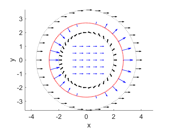
In order to analyze this surprising observation, we consider the simple magnet with continuously rotating dipoles and $k=2$ in Figure 4, where the original dipoles are placed on the inner ring denoted by black dots. Note how the dipoles rotate twice along the ring. The shielding is shown as the red dotted line slightly outside of the original dipoles. The image dipoles, calculated from Equation 3, are shown on the outer dotted ring, where, for $k=2$ they always point to the right. We verify that sum of the original and the image fields is always normal on the shielding, which is shown by the superimposed blue arrows. We also calculate the magnetic field inside the cylindrical shielding, which is shown by the right-pointing arrows near the center. Moreover, inspecting the numerical values shows that the contribution from the images to the field on the inside is negligible.

We conclude that for a continuously varying dipole field shielding the magnet will not affect the magnetic field on the inside. But what about segmented magnets?

4 Shielded and segmented multipoles

Figure 5: Two segments of a segmented multipole that extends radially from $r_{i}$ to $r_{o}$. Each segment has an azimuthal width, given by $2\alpha$. Note the orientation of the easy axis, determined by the tumbling factor $k$, changes from segment to segment.

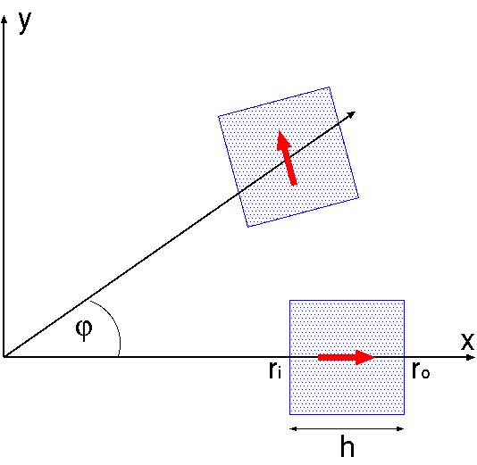
Figure 5 shows two of the segments that are part of a full multipole. We start by calculating the contribution of the field $\underline{B}^{\ast}$ of the segment that is lying on the horizontal axis to the multipoles around $\hat{z}=0$. Rewriting Equation 6 leads to

$${\underline{B}}^{\ast}(\hat{z})=\sum_{m=0}^{\infty}\left\{\frac{m+1}{2\pi}\left[{\underline{B}}_{r}I_{m}+{\underline{B}}_{r}^{\ast}J_{m}\right]\right\}\hat{z}^{m}$$ (9)

where ${\underline{B}}_{r}$ describes the easy axis of the segment on the horizontal axis. The integrals $I_{m}$ and $J_{m}$ are defined by

$$I_{m}=\int_{\Omega}\frac{dxdy}{z^{m+2}}\qquad\mathrm{and}\qquad J_{m}=\frac{1}{R^{2m+2}}\int_{\Omega}\left(z^{\ast}\right)^{m}dxdy\ ,$$ (10)

where $I_{m}$ describes the contribution of the “real” permanent magnets and $J_{m}$ that of their images. We calculate these integrals by suitably parameterizing the trapezoidal region $\Omega$ using the notation introduced in Figure 5, which gives us

$$I_{m} = \int_{r_{i}}^{r_{o}}dx\int_{-x\tan\alpha}^{x\tan\alpha}\frac{dy}{(x+iy)^{m+2}}$$

$$= \frac{-i}{m+1}\int_{r_{i}}^{r_{o}}\frac{dx}{x^{m+1}}\left[\frac{1}{(1+i\tan\alpha)^{m+1}}-\frac{1}{(1-i\tan\alpha)^{m+1}}\right]$$

$$= \frac{2}{m+1}(\cos\alpha)^{m+1}\sin((m+1)\alpha)G_{m}(r_{i},r_{o})\ ,$$

where we introduce the abbreviation $G_{m}(r_{i},r_{o})$ by

$$G_{m}(r_{i},r_{o})=\int_{r_{i}}^{r_{o}}\frac{dx}{x^{m+1}}=\left\{\begin{array}[]{ll}\log(r_{o}/r_{i})&\mathrm{for}\ m=0\\ \frac{1}{m}\left(\frac{1}{r_{i}^{m}}-\frac{1}{r_{o}^{m}}\right)&\mathrm{otherwise.}\end{array}\right.$$ (12)

For the contribution of the image fields we evaluate $J_{m}$ and obtain

$$J_{m} = \frac{1}{R^{2m+2}}\int_{r_{i}}^{r_{o}}dx\int_{-x\tan\alpha}^{x\tan\alpha}(x-iy)^{m}dy$$ (13)

$$= \frac{i}{R^{2m+2}(m+1)}\left[(1-i\tan\alpha)^{m+1}-(1+i\tan\alpha)^{m+1}\right]\int_{r_{i}}^{r_{o}}x^{m+1}dx$$

$$= \frac{2\sin((m+1)\alpha)}{(m+1)(m+2)(\cos\alpha)^{m+1}}H_{m}(r_{i},r_{o},R)$$

with

$$H_{m}(r_{i},r_{o},R)=\frac{1}{R^{2m+2}}\int_{r_{i}}^{r_{o}}x^{m+1}dx=\frac{r_{o}^{m+2}-r_{i}^{m+2}}{R^{2m+2}}\ .$$ (14)

Here we have to keep in mind that for a magnet composed of $M$ segments $2\alpha=2\pi/M$. After inserting $I_{m}$ and $J_{m}$ in Equation 9 we finally obtain

$$\underline{B}^{\ast}(\hat{z})=\sum_{m=0}^{\infty}\left\{{\underline{B}}_{r}g_{m}(\alpha)G_{m}(r_{i},r_{o})+{\underline{B}}_{r}^{\ast}h_{m}(\alpha)H_{m}(r_{i},r_{o},R)\right\}\hat{z}^{m}$$ (15)

with

$$g_{m}(\alpha) = \frac{1}{\pi}(\cos\alpha)^{m+1}\sin((m+1)\alpha)$$

$$h_{m}(\alpha) = \frac{\sin((m+1)\alpha)}{\pi(m+2)(\cos\alpha)^{m+1}}$$ (16)

for the multipole coefficients generated by a single segment.

Figure 6: Segmented dipole (left) and a dipole made of permanent-magnet cubes (right).

In the next step we have to add the contributions of the $M$ segments by noting that each segment $j$ with $0\leq j\leq M-1$ is rotated by an angle $\varphi=2\pi j/M$ with respect to the one lying on the horizontal axis. This changes the integration variable from $z$ to $z^{\prime}=x^{\prime}+iy^{\prime}=e^{i\varphi}(x+iy)=e^{i\varphi}z$. Moreover, the angle of the easy axis changes by $k\varphi$. Thus we can add up contributions from the segments by ornamenting the easy axis $\underline{B}_{r}$ and $\underline{B}_{r}^{\ast}$ in Equation 9 and the integrals $I_{m}$ and $J_{m}$ from Equations 4 and 13 with appropriate phase factors to obtain for the field due to all segments

$$\underline{B}^{\ast}(\hat{z}) = \sum_{m=0}^{\infty}\left\{{\underline{B}}_{r}g_{m}(\alpha)G(r_{i},r_{o})\sum_{j=0}^{M-1}e^{2\pi i(k-m-2)j/M}\right.$$ (17)

$$\qquad\left.+{\underline{B}}_{r}^{\ast}h_{m}(\alpha)H(r_{i},r_{o},R)\sum_{j=0}^{M-1}e^{2\pi i(m-k)j/M}\right\}\hat{z}^{m}\ .$$

The first sum with the exponential factors vanishes unless the $k-m-2$ is a multiple of $M$, or $m=k-2+\nu M$ for some integer $\nu$ in which case the sum evaluates to $M$. Likewise, the second sum vanishes unless $m-k$ is a multiple of $M$, or $m=k+\nu M$. This allows us to write the field from all segments as

$$\underline{B}^{\ast}(\hat{z}) = M\sum_{m=0}^{\infty}\sum_{\nu=0}^{\infty}\left\{{\underline{B}}_{r}g_{m}(\alpha)G_{m}(r_{i},r_{o})\delta_{m,k-2+\nu M}\right.$$ (18)

$$\left.\qquad\qquad+{\underline{B}}_{r}^{\ast}h_{m}(\alpha)H_{m}(r_{i},r_{o},R)\delta_{m,k+\nu M}\right\}\hat{z}^{m}\ ,$$

where $g_{m}(\alpha)$ and $h_{m}(\alpha)$ are defined in Equation 4, $G_{m}(r_{i},r_{o})$ in Equation 12, and $H_{m}(r_{i},r_{o},R)$ in Equation 14.

As an illustration we consider a dipole magnet ($k=2$) made of $M=8$ segments, whose inner radius $r_{i}$ is 10 mm and whose outer radius $r_{o}$ is 20 mm. We assume that the shielding cylinder has a radius of $R=22\,$mm. The main contribution comes from the first term in Equation 18 for $m=0$, in which case $g_{m}(\alpha)=0.115$ with $\alpha=\pi/M$ and $G_{m}(r_{i},r_{o})=\log(2)$. The first term — the dipole — is constant and has magnitude $0.62\underline{B}_{r}$. The smallest non-zero second term is for $m=k=2$, which describes a sextupole. Its magnitude at a radius $|\hat{z}|=r_{i}/2$ becomes $Mh_{2}(\alpha)H(r_{i},r_{o},R){\underline{B}}_{r}^{\ast}(r_{i}/2)^{2}\approx 0.025{\underline{B}}_{r}^{\ast}$ or about 4 % of the dipole component.

For quadrupole magnets ($k=3$) made of $M=8$ magnets and otherwise the same geometry as the dipole from the previous paragraph, we find that the direct field from the “real” permanent magnets at radius $|\hat{z}|=r_{i}/2$ has magnitude $0.38\underline{B}_{r}$ whereas the first contribution (octupolar) of the image fields is $0.005\underline{B}_{r}^{\ast}$, or a little over 1 % of the quadrupole component.

5 Shielded multipoles made of permanent-magnet cubes

Figure 7: Geometry with variables used to calculate the fields of a permanent magnet multipole composed of cubes.

Permanent-magnet cubes are easier to find and less expensive than the trapezoidal segments used in Section 4. We therefore analyze how shielding affects multipoles that are constructed of cubes [10, 12]. The right-hand side in Figure 6 illustrates such a magnet that generates a purely horizontal magnetic field. We calculate the field from Equations 9 and 10 after adapting the integration region $\Omega$ to reflect the cubic shape shown in Figure 7. The first integral $I_{m}$ then becomes

$$I_{m} = \int_{r_{i}}^{r_{o}}dx\int_{-h/2}^{h/2}\frac{dy}{(x+iy)^{m+2}}$$ (19)

$$= \frac{i}{m+1}\int_{r_{i}}^{r_{o}}\left[\frac{1}{(x+ih/2)^{m+1}}-\frac{1}{(x-ih/2)^{m+1}}\right]dx\ .$$

For $m=0$ the integral leads to

$$I_{0} = h\int_{r_{i}}^{r_{o}}\frac{dx}{x^{2}+h^{2}/4}=2\arctan(2r_{o}/h)-2\arctan(2r_{i}/h)$$ (20)

$$= 2\arctan(h^{2}/2\bar{r}^{2})\ ,$$

where we introduce $\bar{r}=(r_{o}+r_{i})/2$ and use the identity $\arctan x-\arctan y=\arctan((x-y)/(1+xy))$ in order to simplify the last equality. For $m=1$ the integral becomes

$$I_{1}=\frac{-h}{2}\left[\frac{1}{r_{o}^{2}+h^{2}/4}-\frac{1}{r_{i}^{2}+h^{2}/4}\right]=\frac{h^{2}\bar{r}}{\bar{r}^{4}+h^{4}/4}\ .$$ (21)

For general $m>0$ we perform the integral over $x$ and then introduce the abbreviations

$$\begin{array}[]{ll}\rho_{o}^{2}=r_{o}^{2}+h^{2}/4\qquad&\rho_{i}^{2}=r_{i}^{2}+h^{2}/4\\ \beta_{o}=\arctan(h/2r_{o})\qquad&\beta_{i}=\arctan(h/2r_{i})\ .\end{array}$$ (22)

This allows us to express $r_{o}\pm ih/2=\rho_{o}e^{\pm i\beta_{o}}$ and $r_{i}\pm ih/2=\rho_{i}e^{\pm i\beta_{i}}$ and turn Equation 19 into

$$I_{m} = \frac{-i}{m(m+1)}\left[\frac{1}{(r_{o}+ih/2)^{m}}-\frac{1}{(r_{i}+ih/2)^{m}}-\frac{1}{(r_{o}-ih/2)^{m}}+\frac{1}{(r_{i}-ih/2)^{m}}\right]$$ (23)

$$= \frac{-i}{m(m+1)}\left[\frac{e^{-im\beta_{o}}-e^{im\beta_{o}}}{\rho_{o}^{m}}-\frac{e^{-im\beta_{i}}-e^{im\beta_{i}}}{\rho_{i}^{m}}\right]$$

$$= \frac{2}{m(m+1)}\left[\frac{\sin(m\beta_{i})}{\rho_{i}^{m}}-\frac{\sin(m\beta_{o})}{\rho_{o}^{m}}\right]\ .$$

For cubic magnets the integral $J_{m}$ corresponding to Equation 13 becomes

$$J_{m} = \frac{1}{R^{2m+2}}\int_{r_{i}}^{r_{o}}dx\int_{-h/2}^{h/2}(x-iy)^{m}dy$$

$$= \frac{-i}{(m+1)R^{2m+2}}\int_{r_{i}}^{r_{o}}\left[(x+ih/2)^{m+1}-(x-ih/2)^{m+1}\right]dx$$

$$= \frac{2}{(m+1)(m+2)}\left[\frac{\rho_{o}^{m+2}}{R^{2m+2}}\sin((m+2)\beta_{o})-\frac{\rho_{i}^{m+2}}{R^{2m+2}}\sin((m+2)\beta_{i})\right]\ ,$$

where $\rho_{o}$, $\rho_{i}$, $\beta_{o}$, and $\beta_{i}$ are defined in Equation 22.

Adding the fields from $M$ cubes with their appropriate rotations progresses in much the same way as in the previous section. The easy axis of $\underline{B}_{r}$ rotates by $e^{2\pi ikj/M}$ and the powers $z$ by $e^{2\pi ij/M}$ for cube number $j$ with $0\leq j\leq M-1$. Again, the sum of the $M$ permanent-magnet cubes becomes zero except for multipoles $m=k-2+\nu M$ and for multipoles $m=k+\nu M$ for the image fields. Only the numerical factors differ from those in Section 4; for the cubes the field thus becomes

$$\underline{B}^{\ast}(\hat{z})=M\sum_{m=0}^{\infty}\sum_{\nu=0}^{\infty}\frac{m+1}{2\pi}\left\{{\underline{B}}_{r}I_{m}\delta_{m,k-2+\nu M}+{\underline{B}}_{r}^{\ast}J_{m}\delta_{m,k+\nu M}\right\}\hat{z}^{m}\ ,$$ (25)

with $I_{m}$ from Equation 20 or 23 and $J_{m}$ from Equation 5.

For a dipole with tumbling factor $k=2$ the direct field from the cubes generates multipoles $m=\nu M$ and the image fields generate multipoles $m=2+\nu M$, such that the two lowest-order contributions are the dipole field $m=0$ from the cubes and $m=2$ from the images. The fields are thus given by

$$\underline{B}^{\ast}(\hat{z}) \approx \frac{M}{2\pi}\left[{\underline{B}}_{r}I_{0}+{\underline{B}}_{r}^{\ast}J_{2}\hat{z}^{2}\right]$$

$$= \frac{M}{\pi}\left[{\underline{B}}_{r}\arctan(h^{2}/2\bar{r}^{2})+{\underline{B}}_{r}^{\ast}\left(\frac{\rho_{o}^{4}}{4R^{6}}\sin(4\beta_{o})-\frac{\rho_{i}^{4}}{4R^{6}}\sin(4\beta_{i})\right)\hat{z}^{2}\right]\ .$$

Notably, the image fields decrease with the sixth power of the radius $R$ of the shielding. Increasing $R$ therefore efficiently helps to reduce the unwanted sextupole component. We refrain from discussing numerical examples, because they are similar to those of segmented magnets from Section 4.

6 Conclusions and outlook

From expressions for the image dipoles outside a magnetically shielding cylinder, we calculated the additional multipole components they cause in Halbach-type multipoles. These additional fields are typically rather small, which can be already expected from the perfect cancellation of the additional fields for a idealized multipole with continuously rotating easy axis (Section 3). But even for segmented or cube-based magnets, the additional fields are small and are attenuated at least by a factor $(\tilde{r}/R)^{6}$ for dipoles and $(\tilde{r}/R)^{8}$ for quadrupoles. Here $\tilde{r}$ typically is the outer radius of the permanent magnet material. Making the shielding cylinder even a little larger thus reduces the additional fields substantially. The multipolarity $m$ of the additional fields is given by $m=k+\nu M$ where $k=2$ for dipoles and $k=3$ for quadrupoles. $M$ is the number of segments or cubes.

In general, Equations 18 and 25 can be used to calculate the multipolarity and the magnitude of the additional fields. Overall, we find that the shielding has a small influence on the field quality in Halbach-type multipoles.

This work was produced in part by Jefferson Science Associates, LLC under Contract No. AC05-06OR23177 with the U.S. Department of Energy. Publisher acknowledges the U.S. Government license and provide public access under the DOE Public Access Plan (http://energy.gov/downloads/doe-public-access-plan).

References

- [1] J. Volk, Experiences with permanent magnets at the Fermilab recycler ring, Journal of Instrumentation 6 (2011) T08003.
- [2] A. Bartnik, N. Banerjee, D. Burke, J. Crittenden, K. Deitrick, J. Dobbins, et al., CBETA: First Multipass Superconducting Linear Accelerator with Energy Recovery, Phys. Rev. Lett. 125, 044803, July 2020.
- [3] T. Watanabe, T. Taniuchi, S. Takano, T. Aoki, and K. Fukami, Permanent magnet based dipole magnets for next generation light sources, Phys. Rev. Accel. Beams 20 (2017) 072401.
- [4] A. Streun, SLS 2.0, The Upgrade of the Swiss Light Source, Proceedings of IPAC 2022, Bangkok, p. 925.
- [5] K. Halbach, Design of Permanent Multipole Magnets with Oriented Rare Earth Cobald Magnets, Nucl. Instrum. Methods 169 (1980) 1.
- [6] OPERA software, https://www.3ds.com/products-services/simulia/products/opera/
- [7] P. Ellaume, O. Chubar, K. Chavanne, Computing 3D magnetic fields from insertion devices, Proceedings of PAC97, p. 3509.
- [8] M. Scheer, UNDUMAG - A new computer code to calculate the magnetic properties of undulators, Proceedings of IPAC2017, p. 3071.
- [9] N. Levinson, R. Redheffer, Complex variables, Holden Day, San Francisco, 1970.
- [10] V. Ziemann, Hands-On Accelerator Physics Using MATLAB, CRC Press, Boca Raton, 2019; especially Sections 4.2 and 4.5.
- [11] R. Plonesy, Current dipole images and reference potentials, IEEE Transactions on bio-medical electronics 10 (1963) 3.
- [12] V. Ziemann, Strap-on magnets: a framework for rapid prototyping of magnets and beam lines, Instruments 5(4) (2021) 36.