Regular Fourier Features for Nonstationary Gaussian Processes

Abstract

Simulating a Gaussian process requires sampling from a high-dimensional Gaussian distribution, which scales cubically with the number of sample locations. Spectral methods address this challenge by exploiting the Fourier representation, treating the spectral density as a probability distribution for Monte Carlo approximation. Although this probabilistic interpretation works for stationary processes, it is overly restrictive for the nonstationary case, where spectral densities are generally not probability measures. We propose regular Fourier features for harmonizable processes that avoid this limitation. Our method discretizes the spectral representation directly, preserving the correlation structure among spectral weights without requiring probability assumptions. Under a finite spectral support assumption, this yields an efficient low-rank approximation that is positive semi-definite by construction. When the spectral density is unknown, the framework extends naturally to kernel learning from data. We demonstrate the method on locally stationary kernels and on harmonizable mixture kernels with complex-valued spectral densities.

1 Introduction

Gaussian processes (GPs) are widely used in fields such as machine learning [rasmussen.2005] and geostatistics [higdon.1998]. Their appeal lies in providing flexible nonparametric regression with principled uncertainty estimates and closed-form computations. While these closed-form solutions are advantageous, they are computationally expensive: simulating a GP at $n$ locations requires decomposing an $n\times n$ covariance matrix, which scales as $\mathcal{O}(n^{3})$ [rasmussen.2005].

Spectral methods offer an efficient alternative by exploiting the Fourier representation of stochastic processes. For stationary GPs, rahimi.2007 introduced random Fourier features (RFFs), which treat the spectral density as a probability distribution and approximate the covariance via Monte Carlo sampling. This yields a low-rank approximation with complexity $\mathcal{O}(nm^{2})$, where $m\ll n$ is the number of features.

Extending RFFs to nonstationary processes is challenging because the spectral density $s(\omega,\omega^{\prime})$ is generally not a probability measure. Existing spectral approaches [samo.2015, ton.2018] require symmetrization and a probability interpretation of the spectral density, limiting the class of representable kernels.

We propose regular Fourier features for harmonizable GPs that avoid these limitations. Our approach discretizes the spectral representation on a regular grid, following the classical Riemann sum approximation of shinozuka.1972 for stationary simulation. The key insight is that for nonstationary processes, the spectral weights at different frequencies are correlated according to the spectral density $s(\omega_{i},\omega_{j})$. By preserving this correlation structure, we obtain a low-rank approximation that is positive semi-definite by construction.

Our contributions are:

• We extend regular Fourier features to harmonizable processes without requiring probability interpretations or symmetrization, which allows one to handle complex-valued spectral densities.

• We introduce a factorized spectral parametrization that guarantees a valid nonstationary kernel by construction and enables learning from data.

• We demonstrate the method on locally stationary kernels and harmonizable mixture kernels with complex-valued spectral densities.

2 Background

We consider harmonizable GPs, a broad class that includes stationary processes as a special case and encompasses many nonstationary processes of practical interest [yaglom.1987, shen.2019]. A zero-mean GP is called harmonizable when it admits the spectral representation [cramer.1942, cramer.1946, loeve.1948]

$$Z(x)=\int_{\mathbb{R}}\exp(\mathrm{i}\omega x)\,\mathrm{d}\Gamma(\omega),$$ (1)

where $\{\Gamma(\omega)\}$ is a complex-valued zero-mean stochastic process indexed by $\omega$, whose spectral distribution

$$S(\omega,\omega^{\prime})=\mathrm{E}[\Gamma(\omega)\,\overline{\Gamma(\omega^{\prime})}],$$ (2)

has bounded variation on $\mathbb{R}\times\mathbb{R}$ [loeve.1948]. The spectral distribution $S$ is positive semi-definite and determines a positive semi-definite kernel $k(x,x^{\prime})=\mathrm{E}[Z(x)\overline{Z(x^{\prime})}]$ via the Fourier-Stieltjes integral [loeve.1948]

$$k(x,x^{\prime})=\iint_{\mathbb{R}^{2}}\exp(\mathrm{i}(\omega x-\omega^{\prime}x^{\prime}))\,\mathrm{d}^{2}S(\omega,\omega^{\prime}).$$ (3)

If the spectral distribution is differentiable, it admits a spectral density $s(\omega,\omega^{\prime})$, and the integral reduces to

$$k(x,x^{\prime})=\iint_{\mathbb{R}^{2}}\exp(\mathrm{i}(\omega x-\omega^{\prime}x^{\prime}))\,s(\omega,\omega^{\prime})\,\mathrm{d}\omega\,\mathrm{d}\omega^{\prime}.$$ (4)

If $\{Z(x)\}$ is stationary, the spectral increments at distinct frequencies are uncorrelated, so the spectral measure concentrates on the diagonal $\omega=\omega^{\prime}$. The kernel then depends only on the lag, and the double integral collapses to

$$k(x-x^{\prime})=\int_{\mathbb{R}}\exp(\mathrm{i}\omega(x-x^{\prime}))\,\mathrm{d}S(\omega),$$ (5)

or, when a spectral density $s(\omega)$ exists

$$k(x-x^{\prime})=\int_{\mathbb{R}}\exp(\mathrm{i}\omega(x-x^{\prime}))\,s(\omega)\,\mathrm{d}\omega.$$ (6)

2.1 Random Fourier Features

For stationary processes, rahimi.2007 observed that the spectral density $s(\omega)$, up to a scaling constant $\sigma^{2}=k(0)$, is a probability density. This allows Monte Carlo approximation of the kernel:

$$k(x-x^{\prime}) \approx\frac{\sigma^{2}}{m}\sum_{j=1}^{m}\exp(\mathrm{i}\Omega_{j}x)\exp(-\mathrm{i}\Omega_{j}x^{\prime})$$

$$=\boldsymbol{\Phi}(x)\boldsymbol{\Phi}(x^{\prime})^{\dagger},$$ (7)

where $\Omega_{j}\sim p(\omega)\propto s(\omega)$, and the feature map is

$$\boldsymbol{\Phi}(x)=\frac{\sigma}{\sqrt{m}}\begin{pmatrix}\exp(\mathrm{i}\Omega_{1}x)&\ldots&\exp(\mathrm{i}\Omega_{m}x)\end{pmatrix}.$$ (8)

The low-rank form $\boldsymbol{\Phi}(x)\boldsymbol{\Phi}(x^{\prime})^{\dagger}$ ensures positive semi-definiteness by construction.

Generalizations to nonstationary processes [samo.2015, ton.2018] require a probability interpretation of $s(\omega,\omega^{\prime})$. A naive Monte Carlo approximation would be

$$k(x,x^{\prime})\approx\frac{\sigma^{2}}{m}\sum_{j=1}^{m}\exp(\mathrm{i}(\Omega_{j}x-\Omega_{j}^{\prime}x^{\prime})),$$ (9)

where $(\Omega_{j},\Omega_{j}^{\prime})\sim p(\omega,\omega^{\prime})\propto s(\omega,\omega^{\prime})$. This approximation is not guaranteed to be positive semi-definite since $\Omega_{j}\neq\Omega_{j}^{\prime}$ in general. This becomes clear by setting $m=1$ and $x=x^{\prime}$:

$$k(x,x)\approx\sigma^{2}\exp(\mathrm{i}(\Omega_{1}-\Omega_{1}^{\prime})x),$$ (10)

which is not guaranteed to be real, let alone nonnegative.

To address this, samo.2015, ton.2018 construct symmetrized feature maps that ensure positive semi-definite approximations, but implicitly constrain the spectral density to a probability measure. Consequently, kernel learning is restricted to this class. When approximating a kernel with a given spectral density, the methods introduce modeling error if the density does not satisfy these assumptions. Alternative spectral approaches [remes.2017, shen.2019] propose parametric kernel families with structured spectral densities for nonstationary kernel learning. In contrast, our approach provides a general kernel decomposition for flexible kernel families, requiring neither symmetrization nor a probability interpretation. Table 1 summarizes the comparison.

A complementary line of work approximates the inference rather than the model. Sparse variational GPs [titsias.2009, hensman.2013] introduce inducing points to approximate the posterior, leaving the kernel unchanged. Variational Fourier features [hensman.2018] replace spatial inducing points with spectral inducing variables within the same variational framework. These inference approximations are orthogonal to our kernel approximation.

3 Regular Nonstationary Fourier Features

We derive regular Fourier features for harmonizable processes by discretizing the spectral representation on an equidistant frequency grid, following the classical simulation idea of shinozuka.1972. While the Riemann sum approximation itself is standard, its extension to harmonizable GPs has not been explored. Unlike random approaches that require a probability interpretation, our method preserves the correlation structure among spectral weights without modifying the spectral density.

Table 1: Comparison of spectral methods for GPs. Checkmarks indicate supported features: nonstationary kernels, unsymmetrized spectral densities (no probability interpretation or symmetrization required), complex-valued spectral densities, and non-compact spectral support. Our method trades non-compact support for the ability to handle arbitrary complex-valued spectral densities.

Method	Nonstationary $k$	Unsymmetrized $s$	Complex $s$	Non-compact $s$
rahimi.2007	✗	–	–	✓
samo.2015, ton.2018	✓	✗	✗	✓
This work	✓	✓	✓	✗

Figure 1: Regular Fourier features approximate the stochastic process $Z(x)$ as a sum of complex exponentials weighted by correlated spectral increments $\mathrm{d}\Gamma(\omega_{k})$. The spectral process (top) is discretized at frequencies $\omega_{1},\ldots,\omega_{m}$. Each harmonic (bottom) shows the contribution $\mathrm{d}\Gamma(\omega_{k})\exp(\mathrm{i}\omega_{k}x)$ in the complex plane.

The spectral representation (1) is a Riemann–Stieltjes integral that can be approximated by a finite sum [loeve.1978] on an equidistant frequency grid with spacing $\Delta\omega=\omega_{k+1}-\omega_{k}$

$$Z(x)\approx\sum_{k=1}^{m}\exp(\mathrm{i}\omega_{k}x)W_{k},$$ (11)

where $W_{k}\coloneqq\Gamma(\omega_{k}+\Delta\omega)-\Gamma(\omega_{k})$ is the spectral increment at frequency $\omega_{k}$. The random variables $W=(W_{1},\ldots,W_{m})^{\top}$ form a zero-mean complex-valued random vector with covariance

$$\mathrm{E}[WW^{\dagger}]\approx\boldsymbol{S}\Delta\omega^{2},\quad[\boldsymbol{S}]_{ij}=s(\omega_{i},\omega_{j}).$$ (12)

In the nonstationary case, the spectral weights $\{W_{k}\}$ are no longer independent but correlated according to the spectral density $s(\omega_{i},\omega_{j})$. This off-diagonal correlation structure encodes the nonstationarity of the process.

Figure 2: Low-rank approximation of the locally stationary kernel showing the sampled spectral density, true kernel, approximation, and absolute error.

When $W$ is complex-valued, its distribution is not fully determined by $\mathrm{E}[WW^{\dagger}]$ alone; the pseudo-covariance $\mathrm{E}[WW^{\top}]$ is also required [lee.1994]. We assume $W$ is circular ($\mathrm{E}[WW^{\top}]=0$) and Gaussian, so that $\mathrm{E}[WW^{\dagger}]\approx\boldsymbol{S}\Delta\omega^{2}$ fully specifies the distribution. Factoring $\boldsymbol{S}\Delta\omega^{2}=\boldsymbol{C}\boldsymbol{C}^{\dagger}$, we write

$$Z(x)\approx\boldsymbol{\alpha}(x)\boldsymbol{C}E=\boldsymbol{\varphi}(x)E,$$ (13)

where $[\boldsymbol{\alpha}(x)]_{k}=\exp(\mathrm{i}\omega_{k}x)$ collects the Fourier basis functions, $\boldsymbol{\varphi}(x)=\boldsymbol{\alpha}(x)\boldsymbol{C}$ is the feature map, and $E=E_{\mathrm{re}}+\mathrm{i}E_{\mathrm{im}}$ is a circularly symmetric complex Gaussian with $E_{\mathrm{re}},E_{\mathrm{im}}\sim\mathcal{N}(\boldsymbol{0},\tfrac{1}{2}\boldsymbol{I})$.

3.1 Low-Rank Kernel Approximation

The kernel $k(x,x^{\prime})=\mathrm{E}[Z(x)\overline{Z(x^{\prime})}]$ admits the low-rank approximation

$$k(x,x^{\prime})\approx\boldsymbol{\varphi}(x)\boldsymbol{\varphi}(x^{\prime})^{\dagger}=\boldsymbol{\alpha}(x)\boldsymbol{C}\boldsymbol{C}^{\dagger}\boldsymbol{\alpha}(x^{\prime})^{\dagger},$$ (14)

which is positive semi-definite by construction since it has the form $\boldsymbol{\Phi}\boldsymbol{\Phi}^{\dagger}$ for any feature matrix $\boldsymbol{\Phi}$. This contrasts with the naive Monte Carlo approximation (9), which lacks this guarantee.

For $n$ sample locations, the kernel matrix $\boldsymbol{K}\in\mathbb{R}^{n\times n}$ is approximated as

$$\boldsymbol{K}\approx\boldsymbol{L}\boldsymbol{L}^{\dagger},\quad[\boldsymbol{L}]_{i}=\boldsymbol{\varphi}(x_{i}),\quad\boldsymbol{L}\in\mathbb{C}^{n\times m}.$$ (15)

Real-Valued Processes

For real-valued processes, the spectral weights satisfy Hermitian symmetry $W_{-k}=\overline{W}_{k}$. Including the spectral mass at the origin, the approximation becomes

$$Z(x) \approx W_{0}+\sum_{k=1}^{m}\exp(\mathrm{i}\omega_{k}x)W_{k}+\exp(-\mathrm{i}\omega_{k}x)\overline{W}_{k}$$

$$=2\,\mathrm{Re}[\tilde{\boldsymbol{\alpha}}(x)W],$$ (16)

where $[\tilde{\boldsymbol{\alpha}}(x)]_{k}=\exp(\mathrm{i}\omega_{k}x)$ for $\omega_{k}\neq 0$ and $1/2$ otherwise. The kernel approximation is

$$k(x,x^{\prime})\approx 2\,\mathrm{Re}[\tilde{\boldsymbol{\varphi}}(x)\,\tilde{\boldsymbol{\varphi}}(x^{\prime})^{\dagger}],\quad\tilde{\boldsymbol{\varphi}}(x)=\tilde{\boldsymbol{\alpha}}(x)\boldsymbol{C}.$$ (17)

When the spectral weights $W_{k}$ are additionally real-valued ($W_{-k}=\overline{W}_{k}=W_{k}$), the positive and negative frequency terms combine to $2\cos(\omega_{k}x)W_{k}$. The feature map then simplifies to $[\tilde{\boldsymbol{\alpha}}(x)]_{k}=\cos(\omega_{k}x)$ for $\omega_{k}\neq 0$ and $1/2$ otherwise, yielding the kernel $k(x,x^{\prime})\approx 4\,\tilde{\boldsymbol{\alpha}}(x)\boldsymbol{C}\boldsymbol{C}^{\top}\tilde{\boldsymbol{\alpha}}(x^{\prime})^{\top}$.

The method extends to $d$ dimensions, for example via product kernels $k(\boldsymbol{x},\boldsymbol{x}^{\prime})=\prod_{p=1}^{d}k(x_{p},x^{\prime}_{p})$, where each dimension uses a one-dimensional spectral density. This preserves computational efficiency at $\mathcal{O}(ndm^{2})$ while allowing dimension-specific nonstationarity.

Assumptions

The method assumes finite spectral support: $s(\omega,\omega^{\prime})=0$ for $|\omega|>\omega_{m}$ or $|\omega^{\prime}|>\omega_{m}$. This band-limited assumption is natural in many applications. When data are sampled at intervals $\Delta x$, the Nyquist theorem limits recoverable frequencies to $\omega_{\text{Nyquist}}=\pi/\Delta x$. Spectral content beyond this is aliased and fundamentally unidentifiable from observations. By setting $\omega_{m}<\omega_{\text{Nyquist}}$, our method avoids modeling high-frequency components that cannot be distinguished from the data. For example, this is particularly relevant in surface texture measurement, where surface textures are inherently band-limited [iso21920-2.2021, iso25178-2.2021].

When the spectral support is not strictly finite, the method introduces truncation error proportional to the spectral mass beyond $\omega_{m}$. If the spectral matrix $\boldsymbol{S}\Delta\omega^{2}$ is ill conditioned, adding a small jitter $\epsilon\,\boldsymbol{I}$ alleviates numerical issues at negligible cost to approximation quality.

Additionally, the finite sum (11) is periodic with period $T=2\pi/\Delta\omega$. Thus, our low-rank approximation actually estimates $\sum_{p,q}k(x-pT,x^{\prime}-qT)$, introducing aliasing error. If the kernel is not zero for $|x|,|x^{\prime}|>\pi/\Delta\omega$, the periods interfere with the approximation. In practice, $\Delta\omega$ should be chosen such that $x_{\max}<\pi/\Delta\omega$, where $x_{\max}=\max_{i}|x_{i}|$.

3.2 Extension to Kernel Learning

When the spectral density is unknown, the framework extends naturally to kernel learning. We focus on real-valued kernels throughout; note that the spectral density $s(\omega,\omega^{\prime})$ can still be complex-valued. A valid spectral density must be positive semi-definite and fulfill

$$s(\omega,\omega^{\prime})=\overline{s(\omega^{\prime},\omega)}=\overline{s(-\omega,-\omega^{\prime})}.$$ (18)

We parametrize the spectral density as

$$s(\omega,\omega^{\prime})=\boldsymbol{f}(\omega)^{\dagger}\boldsymbol{f}(\omega^{\prime})+\boldsymbol{f}(-\omega^{\prime})^{\dagger}\boldsymbol{f}(-\omega),$$ (19)

which is positive semi-definite and Hermitian by construction. The second term enforces the real-kernel symmetry $s(\omega,\omega^{\prime})=\overline{s(-\omega,-\omega^{\prime})}$. Both properties hold for arbitrary $\boldsymbol{f}\colon\mathbb{R}\to\mathbb{C}^{r}$. In matrix form, the spectral matrix is

$$\boldsymbol{S}=\boldsymbol{F}\boldsymbol{F}^{\dagger}+\boldsymbol{F}_{-}\boldsymbol{F}_{-}^{\dagger},$$ (20)

where $[\boldsymbol{F}]_{kj}=\overline{f_{j}(\omega_{k})}$ and $[\boldsymbol{F}_{-}]_{kj}=f_{j}(-\omega_{k})$, both in $\mathbb{C}^{m\times r}$. The function $\boldsymbol{f}$ can be parametrized by a neural network with $2r$ real outputs representing the real and imaginary parts.

Figure 3: Harmonizable mixture kernel approximation with complex-valued spectral density. Top row: real, imaginary, and absolute values of $s(\omega,\omega^{\prime})$. Bottom row: true kernel, approximation, and absolute error.

Inference

Given $n$ observations $\{(x_{i},z_{i})\}_{i=1}^{n}$ and a Gaussian likelihood, we maximize the marginal log-likelihood:

$$\log p(\boldsymbol{z}\mid\Theta)\propto-\boldsymbol{z}^{\top}\boldsymbol{\Sigma}^{-1}\boldsymbol{z}-\log|\boldsymbol{\Sigma}|,$$ (21)

where $\boldsymbol{z}=(z_{1},\ldots,z_{n})^{\top}$, $\boldsymbol{\Sigma}=\boldsymbol{K}+\sigma_{\mathrm{noise}}^{2}\boldsymbol{I}$, and $\Theta$ includes the network parameters and noise variance $\sigma_{\mathrm{noise}}^{2}$.

The factorized form avoids the $\mathcal{O}(m^{3})$ matrix decomposition of $\boldsymbol{S}\Delta\omega^{2}$. Since $\boldsymbol{S}\Delta\omega^{2}=\boldsymbol{F}\Delta\omega(\boldsymbol{F}\Delta\omega)^{\dagger}+\boldsymbol{F}_{-}\Delta\omega(\boldsymbol{F}_{-}\Delta\omega)^{\dagger}$, the decomposition is

$$\boldsymbol{C}=\begin{pmatrix}\boldsymbol{F}&\boldsymbol{F}_{-}\end{pmatrix}\Delta\omega\in\mathbb{C}^{m\times 2r}.$$ (22)

Then the real-valued kernel is $\boldsymbol{K}\approx 2\,\mathrm{Re}[(\tilde{\boldsymbol{\Phi}}\boldsymbol{C})(\tilde{\boldsymbol{\Phi}}\boldsymbol{C})^{\dagger}]$, where $[\tilde{\boldsymbol{\Phi}}]_{ik}=[\tilde{\boldsymbol{\alpha}}(x_{i})]_{k}$ as in (17). Writing $\tilde{\boldsymbol{\Phi}}\boldsymbol{C}=\boldsymbol{A}+\mathrm{i}\boldsymbol{B}$ with real and imaginary parts in $\mathbb{R}^{n\times 2r}$, we obtain $\boldsymbol{K}\approx\boldsymbol{L}\boldsymbol{L}^{\top}$ with

$$\boldsymbol{L}=\sqrt{2}\begin{pmatrix}\boldsymbol{A}&\boldsymbol{B}\end{pmatrix}\in\mathbb{R}^{n\times 4r},$$ (23)

which has rank at most $4r$. Using the Woodbury formula and matrix determinant lemma, the marginal log-likelihood costs $\mathcal{O}(nmr)$ when $r<m\ll n$.

Posterior Prediction

Given $t$ test points, the posterior mean and covariance are

$$\begin{aligned} \boldsymbol{\mu}_{t\mid n}&=\boldsymbol{K}_{t,n}\boldsymbol{\Sigma}^{-1}\boldsymbol{z},\\ \boldsymbol{\Sigma}_{t\mid n}&=\boldsymbol{K}_{t,t}-\boldsymbol{K}_{t,n}\boldsymbol{\Sigma}^{-1}\boldsymbol{K}_{n,t},\end{aligned}$$ (24)

where $\boldsymbol{K}_{t,n}\in\mathbb{R}^{t\times n}$ is the kernel between test and training points. Using the low-rank form $\boldsymbol{K}_{t,n}\approx\boldsymbol{L}_{*}\boldsymbol{L}^{\top}$ with test feature matrix $\boldsymbol{L}_{*}\in\mathbb{R}^{t\times 4r}$, these simplify to $\boldsymbol{\mu}_{*}=\boldsymbol{L}_{*}\boldsymbol{\beta}$ and $\boldsymbol{\Sigma}_{t\mid n}=\boldsymbol{L}_{*}\boldsymbol{Q}\boldsymbol{L}_{*}^{\top}$. Here $\boldsymbol{\beta}=\boldsymbol{L}^{\top}\boldsymbol{\Sigma}^{-1}\boldsymbol{z}\in\mathbb{R}^{4r}$ and $\boldsymbol{Q}=\boldsymbol{I}-\boldsymbol{L}^{\top}\boldsymbol{\Sigma}^{-1}\boldsymbol{L}\in\mathbb{R}^{4r\times 4r}$ are cached during training. Prediction costs $\mathcal{O}(tmr)$, dominated by constructing $\boldsymbol{L}_{*}$.

Figure 4: Ablation studies on the locally stationary kernel showing relative error versus (top) number of features $m$ with fixed $\omega_{m}=5$, and (bottom) cutoff frequency $\omega_{m}$ with fixed $m=100$, across different problem scales $n$.

4 Experiments

We evaluate our approach on both kernel approximation and kernel learning tasks: (1) we demonstrate low-rank approximation quality when the spectral density is known in closed form (Section 4.1), and (2) we show that the factorized parametrization enables learning the Silverman kernel [silverman.1957] from data (Section 4.2).

4.1 Low-Rank Kernel Approximation

We test our kernel approximation on two harmonizable kernels: a locally stationary kernel [silverman.1957] and a harmonizable mixture kernel [shen.2019]. The locally stationary kernel, with its real-valued spectral density, validates approximation quality on a case where existing RFF methods also apply. The harmonizable mixture kernel demonstrates a capability that existing RFF methods fundamentally cannot handle: approximating kernels with complex-valued, unsymmetrized spectral densities.

Figure 5: Posterior predictions on synthetic data from the Silverman locally stationary kernel. Left: true posterior. Center: our method compared to true (dashed). Right: RBF baseline compared to true (dashed).

Locally Stationary Kernel

The locally stationary kernel is [silverman.1957]

$$k_{\mathrm{LS}}(x,x^{\prime})=\exp(-2a\bar{x}^{2})\exp(-\frac{a}{2}\tilde{x}^{2}),$$ (25)

where $\bar{x}=(x+x^{\prime})/2$ is the midpoint, $\tilde{x}=x-x^{\prime}$ is the lag, and $a$ is a kernel parameter. This kernel is harmonizable with real-valued spectral density

$$s_{\mathrm{LS}}(\omega,\omega^{\prime})=\frac{1}{4\pi a}\exp(-\frac{1}{2a}\bar{\omega}^{2})\exp(-\frac{1}{8a}\tilde{\omega}^{2}),$$ (26)

with $\bar{\omega}=(\omega+\omega^{\prime})/2$ and $\tilde{\omega}=\omega-\omega^{\prime}$. This spectral density has the additional property $s(\omega,\omega^{\prime})=s(\omega,-\omega^{\prime})$, so its spectral weights are real-valued: $\overline{W}_{k}=W_{k}$.

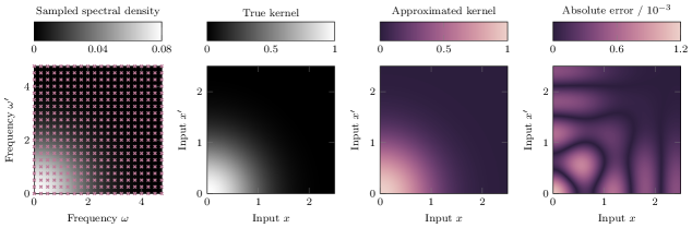
We set $a=1.0$ and approximate the kernel on $x_{i}=i\Delta x$ for $i=0,\ldots,n-1$ with $\Delta x=$0.001$$ and $n=2500$. Using $m=20$ features with cutoff frequency $\omega_{m}=5$ yields spectral spacing $\Delta\omega=$0.25$$. The aliasing condition $\Delta\omega<\pi/(n\Delta x)$ is satisfied. Figure 2 shows (left to right): the spectral density $s_{\mathrm{LS}}(\omega,\omega^{\prime})$ with the $m\times m$ sampling grid overlaid, the true kernel, our low-rank approximation, and the absolute error. The approximation captures the kernel structure accurately, with absolute errors on the order of $10^{-3}$.

Harmonizable Mixture Kernel

We consider a harmonizable mixture kernel (HMK) [shen.2019]. For a single component centered at the origin and no input scaling, the kernel is

$$k_{\mathrm{HMK}}(x,x^{\prime})=k_{\mathrm{LS}}(x,x^{\prime})\sum_{i,j=1}^{Q}B_{ij}\exp\bigl(\mathrm{i}(\eta_{i}x-\eta_{j}x^{\prime})\bigr),$$ (27)

where $\eta_{1},\ldots,\eta_{Q}$ are angular frequencies, $\boldsymbol{B}\in\mathbb{C}^{Q\times Q}$ is a positive semi-definite matrix, and $k_{\mathrm{LS}}$ is the locally stationary kernel defined above. The spectral density is

$$s_{\mathrm{HMK}}(\omega,\omega^{\prime})=\sum_{i,j=1}^{Q}B_{ij}\,s_{\mathrm{LS}}(\omega-\eta_{i},\omega^{\prime}-\eta_{j}),$$ (28)

which can be complex-valued. We use $Q=2$ with conjugate frequencies $\eta_{1}=2\pi$, $\eta_{2}=-2\pi$ and a positive semi-definite matrix

$$\boldsymbol{B}=\begin{pmatrix}2&\frac{1}{2}\mathrm{i}\\ -\frac{1}{2}\mathrm{i}&2\end{pmatrix},$$ (29)

producing a real-valued kernel with a complex-valued spectral density.

To approximate the single-component HMK, we use $m=100$ features with cutoff frequency $\omega_{m}=$20$$ on $x_{i}=i\Delta x$ for $i=-\frac{n-1}{2},\ldots,\frac{n-1}{2}$ with $\Delta x=$0.01$$ and $n=599$. Figure 3 shows the real, imaginary, and absolute values of the spectral density (top row) along with the true kernel, approximation, and absolute error (bottom row). The approximation accurately captures the complex oscillatory structure with absolute errors on the order of $10^{-5}$.

Ablation Studies

To investigate sensitivity to the number of features $m$ and the cutoff frequency $\omega_{m}$, we perform ablation studies on the locally stationary kernel ($a=$1$$) across different problem scales $n\in\{1000,2000,4000,8000\}$ with $\Delta x=$0.001$$. We measure approximation quality using the relative root sum of squared errors.

Figure 4 shows the results. The top panel examines error versus the number of features $m$ with fixed $\omega_{m}=5$, while the bottom panel examines error versus cutoff frequency $\omega_{m}$ with fixed $m=100$. Increasing $m$ consistently reduces approximation error across all problem scales, with diminishing returns beyond $m\approx 160$. For the cutoff frequency, errors decrease as $\omega_{m}$ increases from $4$ to $6$, capturing more spectral content, and plateau beyond $\omega_{m}\approx 8$. Larger problem scales require more features for comparable accuracy, but the overall trends remain consistent.

The value $\omega_{m}=6$ observed in the ablation study corresponds to the point where the spectral density has decayed to negligible levels. For the locally stationary kernel, we have $s_{\mathrm{LS}}(6,6)\approx 10^{-6}\,s_{\mathrm{LS}}(0,0)$, confirming that this cutoff captures most spectral mass. In practice, selecting $\omega_{m}$ is more critical than choosing the number of features $m$. We recommend: (1) set $\omega_{m}$ based on spectral content or the Nyquist limit, then (2) choose $m$ large enough to satisfy the aliasing condition $\Delta\omega<\pi/x_{\max}$.

4.2 Kernel Learning

We generate synthetic observations from the locally stationary kernel (25) with parameter $a=0.5$ on $n=50$ training points uniformly sampled from $-5\leq x\leq 5$. The data are generated by $Z(x)=F(x)+E(x)$ where $F(x)\sim\mathcal{GP}(0,k_{\mathrm{LS}}(x,x^{\prime}))$ is a zero-mean GP and $E(x)$ is white Gaussian noise with standard deviation $\sigma_{\text{noise}}=10^{-2}$.

We parametrize the spectral density using the factorized form (19) with a neural network having two hidden layers of $128$ units each and rank $r=8$. The network outputs $\boldsymbol{f}\colon\mathbb{R}\to\mathbb{R}^{r}$, and we include a learnable global scale parameter $\gamma^{2}$, yielding

$$s(\omega,\omega^{\prime})=\gamma^{2}(\boldsymbol{f}(\omega)^{\top}\boldsymbol{f}(\omega^{\prime})+\boldsymbol{f}(-\omega^{\prime})^{\top}\boldsymbol{f}(-\omega)).$$ (30)

We use $m=255$ features on a symmetric frequency grid with cutoff frequency $\omega_{m}=10$, learning both spectral parameters and noise variance $\sigma_{\mathrm{noise}}^{2}$ via marginal likelihood maximization with AMSGrad [reddi.2018] (learning rate $10^{-2}$, $4000$ iterations).

Across $10$ random seeds, our approach achieves a median relative error of $\qty{66.04}{}$ ($\qtyrange{12.15}{99.97}{}$) compared to $\qty{99.64}{}$ ($\qtyrange{93.32}{138.02}{}$) for the radial basis kernel (RBF) baseline. Half the runs achieved errors $<\qty{50}{}$, demonstrating potential with proper optimization. However, performance exhibits high variance, indicating sensitivity to initialization.

Figure 5 compares posterior predictions for a successful run ($\qty{48.40}{}$ error) on $t=100$ test points for $-10\leq x\leq 10$. The three panels show: (left) the true posterior, (center) our predictions, and (right) RBF baseline predictions, each with mean and $\pm 2\sigma$ uncertainty bands. Our method successfully captures the nonstationary structure. The posterior mean closely follows the true function, and the uncertainty bands match the true bands even in regions without data. In contrast, the RBF kernel fails to capture the correct uncertainty in no-data regimes.

While this parametrization can achieve strong performance, training stability remains a challenge. Developing more robust optimization strategies, such as improved initialization schemes, is an important direction for future work. Despite these challenges, the best-case results demonstrate the potential of the approach for nonstationary kernel learning.

5 Conclusion

We presented a method for constructing regular Fourier features for harmonizable Gaussian processes by discretizing the spectral representation on a regular frequency grid. Unlike existing random Fourier feature approaches for nonstationary kernels, our method does not require the spectral density to be a probability measure or undergo symmetrization.

By factorizing the spectral matrix as $\boldsymbol{S}\Delta\omega^{2}=\boldsymbol{C}\boldsymbol{C}^{\dagger}$, we obtain a low-rank kernel approximation that is positive semi-definite by construction and applies to kernels with arbitrary complex-valued spectral densities. This guarantee arises directly from the factorization structure rather than from symmetrized Monte Carlo sampling. Moreover, the parametrization $s(\omega,\omega^{\prime})=\boldsymbol{f}(\omega)^{\dagger}\boldsymbol{f}(\omega^{\prime})+\boldsymbol{f}(-\omega^{\prime})^{\dagger}\boldsymbol{f}(-\omega)$ emerges naturally and provides a principled framework for kernel learning via marginal likelihood optimization.

We demonstrated high approximation accuracy on the Silverman locally stationary kernel and the harmonizable mixture kernel (complex-valued spectral density), the latter representing a unique capability unavailable to existing RFF methods. For kernel learning, our approach achieved better performance than RBF baselines.

The computational cost scales as $\mathcal{O}(nm^{2})$ for approximation and $\mathcal{O}(nmr)$ for learning, potentially becoming prohibitive for very large datasets. For kernel learning, optimizing the general factorized form remains numerically challenging due to high sensitivity to initialization.

The method assumes finite spectral support, which reflects the reality of discrete sampling: the Nyquist theorem fundamentally limits recoverable frequencies. Additionally, our approach approximates a periodic repetition of the true kernel, requiring the domain to be small enough that successive periods do not overlap.

Future work could examine multi-dimensional settings, develop adaptive frequency selection schemes, derive error bounds, and combine our approach with approximate inference methods.