Certified Circuits:
Stability Guarantees for Mechanistic Circuits

Abstract

Understanding how neural networks arrive at their predictions is essential for debugging, auditing, and deployment. Mechanistic interpretability pursues this goal by identifying circuits—minimal subnetworks responsible for specific behaviors. However, existing circuit discovery methods are brittle: circuits depend strongly on the chosen concept dataset and often fail to transfer out-of-distribution, raising doubts whether they capture concept or dataset-specific artifacts. We introduce Certified Circuits, which provide provable stability guarantees for circuit discovery. Our framework wraps any black-box discovery algorithm with randomized data subsampling to certify that circuit component inclusion decisions are invariant to bounded edit-distance perturbations of the concept dataset. Unstable neurons are abstained from, yielding circuits that are more compact and more accurate. On ImageNet and OOD datasets, certified circuits achieve up to 91% higher accuracy while using 45% fewer neurons, and remain reliable where baselines degrade. Certified Circuits puts circuit discovery on formal ground by producing mechanistic explanations that are provably stable and better aligned with the target concept. Code will be released soon!

(a) Certified circuits, here for ‘African crocodile’,
remove spurious cues. (b) Certified circuits are more compact (x) and
more accurate (y).

Figure 1: Certified circuits are smaller, more accurate, and generalize to OOD. Given a concept dataset, we isolate a circuit—a subnetwork encoding that concept—that is provably stable under dataset edits. (a) Certified circuits keep stable semantic neurons (e.g., teeth) and abstain from unstable spurious ones (e.g., bird cues), improving circuit-only accuracy to $94\%$ ($62\%$ over baseline). (b) Across distribution shifts, ImageNet-discovered certified circuits ($\blacklozenge$) are significantly smaller and more accurate than baseline circuits ($\bullet$).

1 Introduction

Understanding how neural networks arrive at their predictions is a central challenge in machine learning. Mechanistic interpretability tackles this by identifying circuits—minimal subnetworks responsible for specific model behaviors (Olah et al., 2020; Conmy et al., 2023; Elhage et al., 2021). In vision models, for instance, a circuit for recognizing “dog” might comprise particular convolutional filters detecting fur texture, ears, and eyes, connected through specific neurons across subsequent layers. Discovering such circuits promises not only scientific insight into learned representations but also practical benefits: debugging failure modes, auditing for biases, and enabling targeted model editing.

Circuit discovery methods have emerged across modalities. In language models, activation patching and causal tracing isolate attention heads and MLP neurons responsible for factual recall, indirect object identification, and other behaviors (Meng et al., 2022; Wang et al., 2023; Goldowsky-Dill et al., 2023). In vision, analogous methods prune model components to find minimal sufficient subnetworks for recognizing specific visual concepts (Rajaram et al., 2024; Olah et al., 2020; Dreyer et al., 2024). These approaches start with a concept dataset: a collection of inputs representing the target behavior. They then identify which model components are necessary and sufficient to maintain performance on this dataset, discarding the rest. The result is a sparse circuit, i.e., a subgraph of the full model graph that is intended to capture the mechanistic basis of the behavior.

However, current circuit discovery methods lack robustness (Méloux et al., 2025; uit de Bos and Garriga-Alonso, 2024; Miller et al., 2024; Friedman et al., 2024). The identified circuits are sensitive to the choice of concept dataset: adding, removing, or substituting a few semantically equivalent examples can change the discovered circuit unpredictably. They also fail to generalize to out-of-distribution (OOD) data. A circuit found using photographs of dogs on grass may perform poorly on dogs in snow, cartoon dogs, or dogs from unusual angles. Both issues stem from the same underlying problem—current methods overfit to the particular concept dataset rather than recovering the actual concept representation. This undermines confidence in the mechanistic explanation these methods produce.

To address this, we introduce Certified Circuits (Fig.2), a framework that computes the first provable robustness guarantees for circuit discovery. Given a concept dataset

$\mathcal{D}$ and any black-box circuit discovery algorithm, we construct a certified circuit $C^{*}$ with the following guarantee:

Edit distance counts insertions, deletions, or substitutions of examples—so $r=5$ guarantees stability under any combination of up to five such changes. This covers an exponentially large family of datasets.

Our framework is algorithm-agnostic: we (i) randomly subsample the concept dataset several times, (ii) run the base algorithm on each subsample to obtain candidate circuits, and (iii) aggregate votes at the level of individual neurons to determine which components are guaranteed to represent the concept across perturbed datasets. A key byproduct is adaptive sparsity: certification identifies neurons for which no robust decision can be made, yielding circuits that are more compact and accurate than fixed top-$K$ baselines.

In summary, we make the following contributions:

1. We introduce Certified Circuits, the first framework providing provable, algorithm-agnostic robustness guarantees for circuit discovery.

2. We derive provable bounds on certified radii and characterize their dependence on a probability threshold and deletion probability required for subsampling.

3. We demonstrate empirically that certified circuits are more compact, have higher sufficiency, and generalize better to OOD data than uncertified alternatives.

We validate Certified Circuits on ImageNet classification, evaluating sufficiency (does the circuit preserve model behavior?) and compactness (how small can the circuit be while sufficient?) across in-distribution and four OOD benchmarks (OOD-CV, ImageNet-A, ImageNet-O, ImageNet-C). Certified circuits consistently outperform uncertified baselines: certified accuracy improves by up to 91% on OOD data, while circuit size decreases by up to 45%. These gains hold across scoring functions (relevance, activation, rank) used to discover the circuit, confirming that certification captures more transferable mechanistic structure while pruning neurons that are not robustly necessary (Fig. 1). We further analyze whether certified circuits converge to structurally similar solutions when re-discovered on shifted distributions of the same concept. Our Certified Circuits lift classic circuit-based mechanistic explanations to provably robust and more compact explanations that empirically better generalize to OOD data.

2 Related works

2.1 Mechanistic Interpretability

Mechanistic interpretability aims to reverse-engineer the internal computations of neural networks, moving beyond input-output behavior to understand how models arrive at their predictions (Olah et al., 2020; Elhage et al., 2021; Bereska and Gavves, 2024). The field spans observational methods that analyze learned representations (e.g., probing, sparse autoencoders) and interventional methods that causally localize computations through targeted ablations and activation patching (Zeiler and Fergus, 2014; Zimmermann et al., 2021; Meng et al., 2022).

Circuit discovery. Circuit discovery aims to identify minimal subnetworks (circuits) that implement a target behavior or concept. Circuit nodes can be feature channels in CNNs, attention heads in transformers, or MLP neurons, depending on the chosen granularity (Bereska and Gavves, 2024). Typically, one (i) defines a concept via a dataset, (ii) represents the model as a computational graph with nodes and edges connecting them, and (iii) extracts a sparse subgraph whose components are necessary and/or sufficient for that behavior (Conmy et al., 2023). In language models, this approach has revealed circuits for factual recall (Meng et al., 2022), indirect object identification (Wang et al., 2023), and most recently for verifying chain-of-thought reasoning (Zhao et al., 2025). ACDC (Conmy et al., 2023) automates discovery via iterative edge pruning. In vision, circuits have been studied via feature-preserving subnetworks (Hamblin et al., 2022), connectivity-based tracing of concept-specific computations (Rajaram et al., 2024; Wang et al., 2019), disentanglement of polysemantic neurons into concept circuits (Dreyer et al., 2024), and qualitative connectome-style visualizations spanning all layers (Kowal et al., 2024).

Stability limitations. A core limitation is that discovered circuits can be highly unstable: swapping in different (but semantically equivalent) examples to represent the same concept (or making small additions/removals) can yield substantially different circuit. This raises a basic question: is the circuit capturing the concept, or overfitting to dataset-specific spurious cues? Recent work documents and diagnoses such fragility. Méloux et al. (2025) cast circuit discovery as statistical estimation and show that EAP-IG (transformer circuit discovery method) circuits can change markedly even when the same behavior is defined using paraphrased prompt sets, indicating high variance in the discovered structure. Miller et al. (2024) further find that common circuit faithfulness metrics are not robust to evaluation choices. Finally, Friedman et al. (2024) show that explanations can appear faithful on the discovery distribution yet fail to generalize, creating interpretability illusions.

These works highlight the problem but do not provide solutions that rule out instability. Concurrent work uses neural network verification to certify the faithfulness of a fixed circuit under small input-level perturbations (Anonymous, 2026); in contrast, our concern is dataset-to-circuit instability, where the discovered circuit itself changes when the concept dataset is edited. To our knowledge, no prior method certifies invariance of circuit structure under bounded dataset-level perturbations.

2.2 Robustness Certification

A robustness certificate is a worst-case guarantee of output invariance: given an input $x$ and a radius $r$, the certified model provably returns the same prediction for every perturbed input $x^{\prime}$ with $\mathrm{dist}(x,x^{\prime})\leq r$ (otherwise it abstains). Randomized smoothing yields such certificates by aggregating the base model’s predictions under random perturbations and converting the resulting probability margin into a certified radius (Lécuyer et al., 2019; Cohen et al., 2019; Anani et al., 2025). Beyond single-label classification, smoothing has been extended to (i) structured outputs via per-component abstention, certifying only confident components in segmentation settings (Fischer et al., 2021; Anani et al., 2024), and (ii) discrete objects under edit distance, where RS-Del uses randomized deletions to certify invariance against insertions, deletions, and substitutions within an edit budget (Huang et al., 2023). We build on these ideas to certify circuit component stability under dataset-level edit perturbations.

Summary. Circuit discovery is unstable: small edits to the concept dataset, even replacing examples with semantically equivalent ones, can produce entirely different circuits, blurring whether the circuit encodes the concept or dataset-specific artifacts. We address this by certifying the dataset-to-circuit mapping: using deletion-based smoothing (RS-Del) (Huang et al., 2023) to model bounded dataset edits, together with circuit component-level certification to exclude the unstable circuit components (Fischer et al., 2021), we return certified circuits whose certified nodes are provably invariant to edits within an edit-distance budget.

3 Certified Circuits

To overcome the circuit instability in prior work, we formalize circuit discovery as a dataset-level mapping and ask: which circuit components are provably stable under bounded edits to the concept dataset? Our approach is driven by three goals. First, we seek guarantees (not empirical heuristics) that circuit structure is invariant, ruling out brittleness by construction. Second, edit distance provides a threat model: it captures the scenario where a practitioner adds examples, removes outliers, or swaps in semantically equivalent images, and expects the discovered circuit to remain unchanged if it encodes the concept. Third, stability under such edits is a prerequisite for out-of-distribution generalization: a circuit that changes when the concept dataset is perturbed cannot be expected to transfer to shifted test distributions. Enumerating all bounded-edit datasets is infeasible, so we use randomized smoothing: we run circuit discovery on many random subsamples and aggregate the outcomes to certify stability for all edits within the radius.

Figure 2: Certified circuit discovery via concept deletion smoothing. (§3.1) Given a concept dataset $\mathcal{D}$, model graph $G$, and circuit discovery algorithm $A$: (§3.2) We sample dataset variants via per-example random deletion with probability $p_{\mathrm{del}}$, (§3.3) run $A$ on each to obtain candidate circuits, (§3.4) aggregate per-vertex inclusion frequencies, (§3.4) certify vertices as in, out, or abstain ($\oslash$) based on votes consistency. (§3.5) The certified circuit is provably invariant to dataset edits within radius $r$.

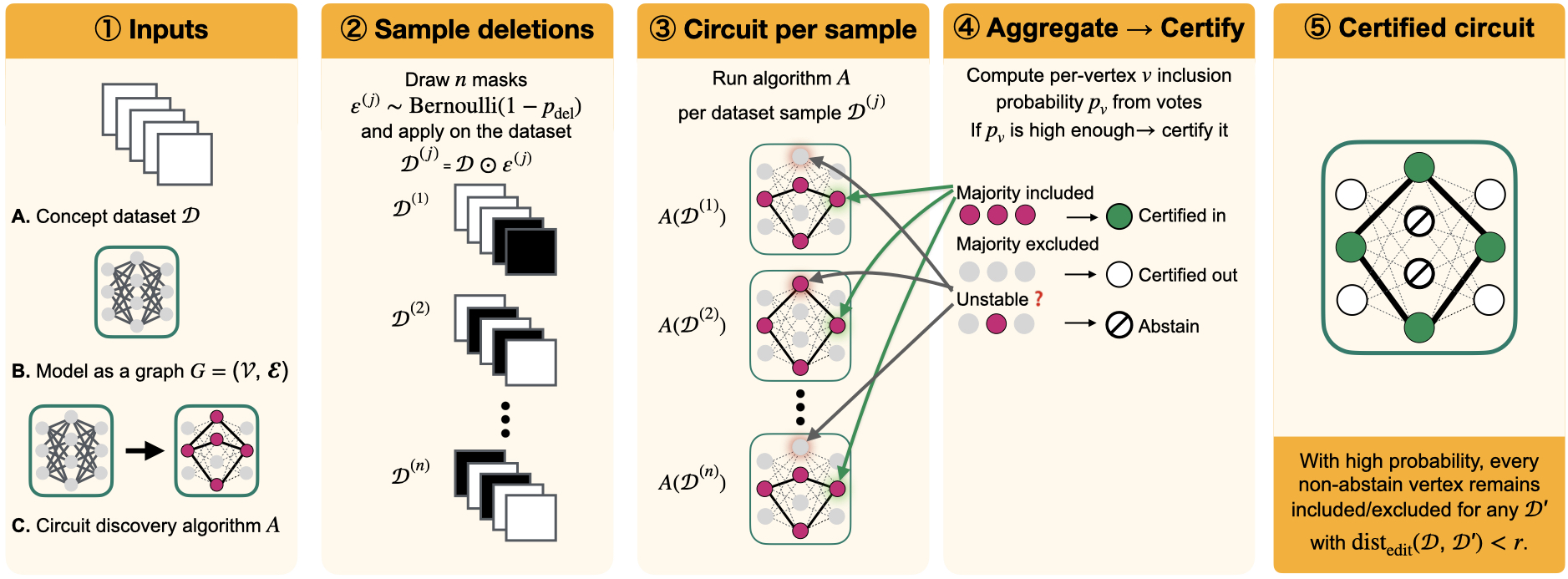
Our approach (Figure 2). Given a model graph $G{=}(\mathcal{V},\mathcal{E})$, a concept dataset $\mathcal{D}$, and any black-box circuit discovery algorithm $A$, we certify which circuit components (vertices $v\in\mathcal{V}$) are provably stable under bounded dataset edits. After briefly reviewing randomized smoothing, we formalize our setup (§3.1). We then define dataset deletion smoothing (RS-Del (Huang et al., 2023); §3.2) and a smoothed circuit discovery rule that aggregates vertex-wise inclusion probabilities and thresholds them to output certified in/out or abstain (§3.3). We present Theorem 3.3, which guarantees certified decisions are invariant for all datasets within edit-distance $r$. Finally, we describe the Monte Carlo estimation of the certified circuit discovery algorithm (§3.4) and summarize its key properties (§3.5).

Background: Randomized Smoothing

We introduce randomized smoothing (Lécuyer et al., 2019; Cohen et al., 2019) as the main technical tool for turning empirical stability under random perturbations into certified robustness guarantees. Let $f_{b}:\mathcal{X}\to\mathcal{Y}$ be a base classifier and let $\phi:\mathcal{X}\to D(\mathcal{X})$ be a perturbation mechanism that maps an input $x$ to a distribution $\phi(x)$ over perturbed inputs. Randomized smoothing defines the smoothed classifier

$$f(x):=\arg\max_{y\in\mathcal{Y}}\mathbb{P}_{z\sim\phi(x)}\!\left[f_{b}(z)=y\right].$$ (1)

A certificate is obtained by lower-bounding the probability of the predicted class and deriving a radius $r$ such that, with confidence at least $1-\alpha$, the prediction is invariant within the corresponding neighborhood, i.e., $f(x)=f(x^{\prime})$ for all $x^{\prime}$ satisfying $\mathrm{dist}(x,x^{\prime})\leq r$.

3.1 Setup and Inputs

Let $G=(\mathcal{V},\mathcal{E})$ denote the model, represented as a directed graph whose vertices $\mathcal{V}$ are circuit components (e.g., neurons, attention heads) and whose edges $\mathcal{E}$ represent connections between components. Our method operates on a concept dataset $\mathcal{D}=(x_{1},\ldots,x_{|\mathcal{D}|})\in\mathcal{X}^{*}$, viewed as a finite sequence of inputs that contain the same concept (e.g., same-class images).

Assume any black-box circuit discovery algorithm $A$ that maps a concept dataset to a binary mask over vertices,

$$A:\mathcal{X}^{*}\;\longrightarrow\;\{0,1\}^{|\mathcal{V}|},$$ (2)

where $A_{v}(\mathcal{D})=1$ indicates that vertex $v\in\mathcal{V}$ is included in the circuit associated with $\mathcal{D}$ and $A_{v}(\mathcal{D})=0$ indicates exclusion. A common example of algorithm $A$ is a top-$K$ circuit rule: for each layer, score vertices on $\mathcal{D}$ (e.g., by mean activation or gradient-based relevance) and include the $K$-fraction highest-scoring vertices, yielding a sparse mask over components $v\in\mathcal{V}$ (Olah et al., 2020; Hamblin et al., 2022; Rajaram et al., 2024; Dreyer et al., 2024).

The goal is to construct a smoothed (certified) variant $\tilde{A}^{\tau}$ of $A$ whose component-wise decisions are provably stable under bounded edit perturbations of $\mathcal{D}$.

3.2 Dataset Deletion Smoothing

To certify robustness of circuit discovery under dataset-level edits, we model the concept dataset $\mathcal{D}=(x_{1},\ldots,x_{|\mathcal{D}|})$ as a sequence and measure perturbations via edit distance $\mathrm{dist}_{\mathrm{edit}}(\mathcal{D},\mathcal{D}^{\prime})$, counting insertions, deletions, and substitutions required to transform $\mathcal{D}$ to $\mathcal{D}^{\prime}$. Directly checking stability under all edits is intractable; instead, following RS-Del (Huang et al., 2023), we use randomized deletions as a smoothing perturbation, which nevertheless yields certificates with respect to the full edit distance. Although concept datasets are naturally unordered, we fix an arbitrary ordering solely to define $\mathrm{dist}_{\mathrm{edit}}$; this does not affect the certificate since our base algorithms $A$ depend only on permutation-invariant statistics.

Concretely, we define a deletion-based perturbation distribution $\phi_{p_{\mathrm{del}}}(\mathcal{D})$ by sampling an i.i.d. binary mask

$$\varepsilon=(\varepsilon_{1},\ldots,\varepsilon_{|\mathcal{D}|}),\qquad\varepsilon_{i}\sim\mathrm{Bernoulli}(1-p_{\mathrm{del}}),$$

where $\varepsilon_{i}=1$ keeps $x_{i}$ and $\varepsilon_{i}=0$ deletes it. We treat the concept dataset as an ordered sequence $\mathcal{D}=(x_{1},\ldots,x_{|\mathcal{D}|})$ (e.g., in dataset index order), so applying $\varepsilon$ produces an ordered subsequence:

$$\mathcal{D}\odot\varepsilon =(x_{i}\mid\varepsilon_{i}=1)$$

$$=(x_{i_{1}},\ldots,x_{i_{m}}),\quad\text{with }1\leq i_{1}<\cdots<i_{m}\leq|\mathcal{D}|.$$

The random sub-dataset $\mathcal{D}\odot\varepsilon$ is distributed according to $\phi_{p_{\mathrm{del}}}(\mathcal{D})$. This perturbation model is the input-side mechanism underlying our certified guarantees, and it directly connects our setting to RS-Del’s edit-distance certification under deletion-based smoothing (Huang et al., 2023).

3.3 Smoothed Circuit Discovery

Given a base circuit discovery algorithm $A$ and the deletion perturbation distribution $\phi_{p_{\mathrm{del}}}(\mathcal{D})$, we define the smoothed circuit discovery algorithm

$$\tilde{A}^{\tau}:\mathcal{X}^{*}\to\{0,1,\oslash\}^{|\mathcal{V}|},$$

which returns for each vertex $v\in\mathcal{V}$ one of three outcomes: certified in (1), certified out (0), or abstain ($\oslash$). The confidence threshold $\tau\in[0.5,1)$ controls how much posterior mass is required to make a non-abstaining decision: if neither inclusion nor exclusion is sufficiently likely under randomized deletions, the method abstains.

To define $\tilde{A}^{\tau}$, we quantify how consistently the base algorithm $A$ includes a vertex under randomized deletions. For a vertex $v$, we define the smoothed inclusion probability:

$$p_{v}(\mathcal{D}) =\mathbb{P}_{\varepsilon}\!\left[A_{v}\!\big(\mathcal{D}\odot\varepsilon\big)=1\right],$$ (3)

$$\qquad\varepsilon_{i}\sim\mathrm{Bernoulli}(1-p_{\mathrm{del}})\ \text{i.i.d.}$$

i.e., the probability that $A$ includes $v$ when run on a randomly deleted sub-dataset $\mathcal{D}\odot\varepsilon$. Values near $1$ mean $v$ is selected almost always (stable inclusion), while values near $0$ mean it is rarely selected (stable exclusion).

The smoothed algorithm $\tilde{A}^{\tau}$ converts these probabilities into certified per-vertex decisions by requiring a margin of at least $\tau$ in favor of inclusion or exclusion. Following segmentation-style smoothing (Fischer et al., 2021), we set

$$\tilde{A}^{\tau}_{v}(\mathcal{D})=\begin{cases}1&\text{if }p_{v}(\mathcal{D})>\tau,\\ 0&\text{if }1-p_{v}(\mathcal{D})>\tau,\\ \oslash&\text{otherwise},\end{cases}$$ (4)

so $\tilde{A}^{\tau}_{v}(\mathcal{D})=1$ certifies that $v$ is robustly included, $\tilde{A}^{\tau}_{v}(\mathcal{D})=0$ certifies that it is robustly excluded, and $\tilde{A}^{\tau}_{v}(\mathcal{D})=\oslash$ abstains when neither decision has enough evidence. We write $\tilde{A}^{\tau}(\mathcal{D}):=(\tilde{A}^{\tau}_{v}(\mathcal{D}))_{v\in\mathcal{V}}\in\{0,1,\oslash\}^{|\mathcal{V}|}$ for the resulting three-valued mask over all vertices.

Guarantees. The rule defining $\tilde{A}^{\tau}$ converts vote consistency under randomized deletions into a worst-case guarantee over all datasets within an edit-distance neighborhood of $\mathcal{D}$. Combining RS-Del (Huang et al., 2023) with component-wise certification (Fischer et al., 2021) yields a certified stability guarantee for every non-abstaining vertex:

The guarantee in Theorem 3.3 states that any vertex that $\tilde{A}^{\tau}$ certifies as in ($1$) or out ($0$) of the circuit remains so for all concept datasets $\mathcal{D}^{\prime}$ with $\mathrm{dist}_{\mathrm{edit}}(\mathcal{D},\mathcal{D}^{\prime})<r$, with confidence at least $1-\alpha$. Vertices assigned $\oslash$ are excluded from the certified circuit. The proof is in App. A.

From certified mask to a circuit. Given the per-vertex guarantee in Theorem 3.3, we can now formally define the certified circuit itself. The certified output $\tilde{A}^{\tau}(\mathcal{D})\in\{0,1,\oslash\}^{|\mathcal{V}|}$ is a vertex-wise mask, so we construct a circuit as the subgraph induced by the vertices certified as included:

$$\mathcal{V}^{*} =\{v\in\mathcal{V}\mid\tilde{A}^{\tau}_{v}(\mathcal{D})=1\},$$

$$\mathcal{E}^{*} =\{(u,v)\in\mathcal{E}\mid u\in\mathcal{V}^{*}\land v\in\mathcal{V}^{*}\},$$

$$C^{*} =(\mathcal{V}^{*},\mathcal{E}^{*}).$$

Thus $C^{*}$ contains all certified-in vertices and all edges between them, while vertices assigned $\oslash$ are excluded since their membership cannot be certified stable.

3.4 Estimating the Certified Circuit

In practice, the probabilities $p_{v}(\mathcal{D})$ (Eq. 3) are unknown and are estimated by Monte Carlo sampling: draw $n$ i.i.d. deletion masks $\varepsilon^{(1)},\ldots,\varepsilon^{(n)}\sim\mathrm{Bernoulli}(1-p_{\mathrm{del}})^{|\mathcal{D}|}$, evaluate $A_{v}(\mathcal{D}\odot\varepsilon^{(j)})$ for each $j$, and use the resulting empirical frequency to estimate the lower bound of $p_{v}(\mathcal{D})$, from which a $(1-\alpha)$ lower confidence bound is computed to decide whether $\tilde{A}_{v}^{\tau}(\mathcal{D})\in\{0,1\}$ or $\oslash$. We follow the standard evaluation scheme as in (Fischer et al., 2021).

3.5 Properties of Certified Circuits

Smoothed circuit discovery yields certified circuits with three key properties: (i) provable dataset-level stability: all non-abstain certified vertices are invariant under any sequence of fewer than $r$ dataset edits; (ii) spurious-feature suppression: vertices whose membership decisions are unstable across deletions are abstained from, producing strictly sparser circuits; and (iii) algorithm and model agnosticism: our framework wraps any circuit discovery method $A$ and model $G$ without requiring access to its internals. Next, we will discuss that Certified Circuits also have practical benefits, better capturing the target concept prediction and generalizing well to OOD data.

4 Experimental Setup

Baseline circuit discovery algorithms. We evaluate our certification framework using a standard top-$K$ based circuit discovery flow (Hamblin et al., 2022; Conmy et al., 2023; Rajaram et al., 2024; Dreyer et al., 2024). Given a model, we define circuit vertices as feature channels at the output of each residual block. For each concept dataset, we score every vertex and retain the top-$K$ fraction per layer (i.e., the $K\cdot|\text{channels}|$ highest-scoring channels) according to one of three scoring functions, which defines our base circuit discovery algorithm $A$ (Eq. 2). As scores we consider (i) Activation: mean activation magnitude over the concept dataset; (ii) Relevance: mean attribution score; or (iii) Rank: per-image ranking of vertices by activation, aggregated across the dataset. Because certification abstains from unstable vertices, the certified circuit is typically smaller than the initial top-$K$ selection; therefore, whenever we report $K$ for certified circuits we report the effective retained fraction after abstention (not the base algorithm’s target $K$).

Datasets and architectures. We use ImageNet (Russakovsky et al., 2015) as an in-distribution benchmark, with each class as a concept dataset $\mathcal{D}$ by collecting a set of same-class images. Circuits are discovered on 100 randomly selected classes and evaluated under four OOD shifts: OOD-CV, where objects appear in novel contexts and backgrounds (Zhao et al., 2022); ImageNet-A, consisting of naturally occurring adversarial examples (Hendrycks et al., 2019); ImageNet-O, containing object categories absent from ImageNet (Hendrycks et al., 2019); and ImageNet-C (defocus blur), a corruption shift induced by optical blur (Hendrycks and Dietterich, 2019). We run experiments on ResNet-50 and ResNet-101 (He et al., 2016), selecting circuit vertices from the outputs of their four residual blocks (256, 512, 1024, and 2048 channels, respectively).

Sufficiency. We measure circuit sufficiency by whether the model’s prediction is preserved when computation is restricted to the discovered circuit. This sufficiency pruning evaluation is standard in circuit discovery: one ablates all non-circuit components (or equivalently, runs the model with only the circuit active) and measures task performance using the remaining subnetwork (Conmy et al., 2023; Meng et al., 2022; Wang et al., 2023; Dreyer et al., 2024). Concretely, for a circuit $C_{c}$ discovered for class $c$, we zero all non-circuit channels at each residual block and evaluate the pruned model on the corresponding concept dataset $\mathcal{D}_{c}$. We report mean circuit class accuracy (cACC), the average classification accuracy across evaluated classes:

$$\mathrm{cACC}:=\frac{1}{|\mathcal{Y}|}\sum_{c\in\mathcal{Y}}\mathrm{CA}(C_{c},\mathcal{D}_{c}),$$ (6)

where $\mathcal{Y}$ is the set of evaluated classes and $\mathrm{CA}(C_{c},\mathcal{D}_{c})$ is the classification accuracy of the pruned model (retaining only $C_{c}$) on $\mathcal{D}_{c}$.

Certification hyperparameters. The choice of $p_{\mathrm{del}}$ and $\tau$ is critical: high $p_{\mathrm{del}}$ deletes too much data, hindering the base algorithm, while high $\tau$ demands excessive confidence for certification, which increases the abstain rate. We analyze the certified radius $r$ in App. B (Figure 5). Based on this analysis, we set $p_{\mathrm{del}}=0.6$ and $\tau=0.95$, yielding certified radius $r=1$. We use $n=1000$ Monte Carlo samples and failure probability $\alpha=0.001$, following the standard setting in randomized smoothing literature (Lécuyer et al., 2019; Cohen et al., 2019; Anani et al., 2025). All certified results are guaranteed with confidence $1-\alpha$.

Paradigm	Scoring Top-$K$	In-Distribution		Out-of-Distribution
		ImageNet		OOD-CV		ImageNet-A		ImageNet-O		ImageNet-C
		$\mathrm{cACC}\uparrow$	$K\downarrow$	$\mathrm{cACC}\uparrow$	$K\downarrow$	$\mathrm{cACC}\uparrow$	$K\downarrow$	$\mathrm{cACC}\uparrow$	$K\downarrow$	$\mathrm{cACC}\uparrow$	$K\downarrow$
Model	–	81	1.00	20	1.00	9	1.00	81	1.00	59	1.00
Baseline circuit	Relevance	86	0.70	74	0.40	62	0.40	93	0.60	74	0.70
	Activation	83	0.80	37	0.40	19	0.60	87	0.70	68	0.70
	Rank	47	0.70	40	0.40	16	0.60	60	0.70	43	0.70
Certified circuit (ours)	Relevance	96 $\uparrow\!12\%$	0.34 $\downarrow\!51\%$	93 $\uparrow\!25\%$	0.34 $\downarrow\!16\%$	94 $\uparrow\!51\%$	0.34 $\downarrow\!14\%$	98 $\uparrow\!6\%$	0.42 $\downarrow\!30\%$	93 $\uparrow\!26\%$	0.34 $\downarrow\!51\%$
	Activation	84 $\uparrow\!1\%$	0.61 $\downarrow\!24\%$	53 $\uparrow\!46\%$	0.27 $\downarrow\!33\%$	37 $\uparrow\!91\%$	0.33 $\downarrow\!45\%$	90 $\uparrow\!3\%$	0.49 $\downarrow\!30\%$	72 $\uparrow\!6\%$	0.50 $\downarrow\!28\%$
	Rank	83 $\uparrow\!76\%$	0.69 $\downarrow\!1\%$	46 $\uparrow\!16\%$	0.38 $\downarrow\!4\%$	28 $\uparrow\!72\%$	0.58 $\downarrow\!3\%$	90 $\uparrow\!50\%$	0.57 $\downarrow\!18\%$	71 $\uparrow\!66\%$	0.58 $\downarrow\!17\%$

Table 1: Certified vs. baseline circuit sufficiency. Peak cACC and corresponding circuit size $K$ under sufficiency pruning on ResNet-101. Circuits are discovered on ImageNet and evaluated either in-distribution or on OOD shifts.

5 Results

We evaluate Certified Circuits in three ways: circuit sufficiency and compactness (§5.1), testing whether circuits preserve class predictions when used in isolation and how small they can be; out-of-distribution generalization (§5.2), measuring whether circuits discovered in-distribution retain accuracy under distribution shift; and structural stability (§5.3), assessing whether circuit structure remains consistent when re-discovered on shifted data.

Figure 3: Circuit accuracy (cACC) vs. size $K$. Solid lines show certified circuits, dashed show baselines, with colors distinguishing models. Rows vary scoring methods, columns vary datasets. Circuits are discovered on ImageNet and evaluated on OOD data.

5.1 Circuit Sufficiency and Compactness

We study two questions: (i) sufficiency: does the circuit alone preserve the target class prediction? and (ii) compactness: how small can the circuit be while remaining sufficient? We sweep the circuit size $K\in(0,1]$ (fraction of channels retained), and report (a) the peak cACC over $K$ and the corresponding $K$ (Table 1), as well as (b) the full cACC–$K$ curves (Fig. 3) across five test datasets and three scoring rules (Relevance, Activation, Rank).

Sufficiency. Does using the circuit alone preserve the class prediction? We evaluate circuit sufficiency via peak cACC (Eq. 6) in Table 1 and cACC across circuit sizes $K$ in Figure 3. In general, certified circuits consistently outperform baselines across all five datasets and all three scoring algorithms. On ImageNet, certified circuits ($96\%$ peak cACC) increase upon the baseline ($86\%$) by $12\%$. Importantly, the accuracy on non-target class images is decreased for certified circuits. Thus, they yield more class-specific circuits, even on OOD data (see App. C).

Compactness. How small can the circuit be while sufficient? We assess compactness by the circuit size $K$ at which peak mean class accuracy (cACC) is achieved. Table 1 and Figure 3 show that certified circuits generally reach peak cACC at substantially smaller $K$ than baseline circuits. On ImageNet, the certified circuit is $51\%$ smaller while improving peak cACC by $12\%$.

Effect of compactness on sufficiency. In Figure 3 we show cACC against circuit size $K\in(0,1)$ across all five datasets. Both certified and baseline circuits follow a three-stage pattern as $K$ increases: (i) small $K$ yields insufficient circuits that omit class-critical neurons, low cACC, (ii) intermediate $K$ captures the necessary class evidence and cACC peaks, (iii) large $K$ introduces competing or spurious features, reducing class specificity and degrading cACC. Crucially, certified circuits shift this curve favorably in both dimensions: they peak at smaller $K$ (more compact) and achieve higher cACC at that peak (more sufficient). This means certification does not trade off one property for the other. Certification appears to prune those neurons that are unnecessary (enabling compactness) and harmful to the accuracy (enabling sufficiency) at the same time.

Certified circuits are more accurate at smaller size.

5.2 Out-of-Distribution Generalization

Do circuits discovered in-distribution retain their class accuracy on shifted data? We evaluate OOD generalization by discovering class-specific circuits on ImageNet and using these circuits to classify corresponding classes in shifted datasets by measuring cACC.(Table 1, Figure 3).

In general, certified circuits retain substantially higher cACC than baselines under distribution shifts, with the largest gains on the hardest shifts. Specifically, on OOD-CV (context and background shift), certified circuits reach $93\%$ cACC at $K{=}0.34$ versus $74\%$ at $K{=}0.40$ for the baseline ($25\%$ increase), while the unmodified model ($K{=}1.0$) drops to ${\sim}20\%$. On ImageNet-A (natural adversarial examples), certified circuits achieve $94\%$ at $K{=}0.34$ versus $62\%$ baseline ($51\%$ increase), whereas the full model attains only ${\sim}9\%$. On ImageNet-C (corruption), certified circuits improve by $26\%$ over baseline while using $51\%$ fewer neurons.

These results suggest certified circuits capture class-relevant features that transfer across shifts. Abstention removes neurons whose inclusion is inconsistent under dataset perturbations, which are likely spurious rather than concept-based. Pruning these unstable components yields circuits that generalize beyond the discovery distribution and outperform both baselines and the full network.

Certified circuits generalize to OOD shifts.

5.3 Structural Stability Under Distribution Shift

The previous experiments used the same circuit on different distributions. A stronger test asks: does the certified circuit structure remain stable beyond the certified radius, when re-discovered on different distributions of the same concept? We measure this via IoU between circuits discovered on ImageNet and re-discovered on each shifted dataset, at the $K$ maximizing the certified–baseline cACC gap (Fig. 4). For two circuits with vertices sets $V$ and $V^{\prime}$, the IoU is defined $|V\cap V^{\prime}|/|V\cup V^{\prime}|$.

Figure 4: Structural stability under distribution shift. Per-class IoU between circuits discovered on ImageNet and re-discovered on each OOD dataset, evaluated at the $K$ that maximizes the certified–baseline $\Delta$cACC = $100\cdot\frac{\mathrm{cACC}_{\mathrm{cert}}-\mathrm{cACC}_{\mathrm{base}}}{\mathrm{cACC}_{\mathrm{base}}}$ gap. Boxes show the distribution over classes. Relevance top-$K$ scoring is used.

Overall, certified circuits have higher median IoU and tighter distributions than baselines across shifts, indicating more consistent structure. The largest stability gains align with the largest $\Delta cACC$ performance gains on OOD-CV $104\%$ and ImageNet-A $83\%$. ImageNet-O is the exception, where both methods show high variance, suggesting class-dependent circuit reconfiguration under semantic anomalies.

These findings reinforce the OOD generalization results: abstention suppresses shift-sensitive vertices, concentrating circuits on an invariant core that better captures the underlying concept rather than distribution-specific artifacts.

Certified circuits converge to a similar invariant core when re-discovered on shifted distributions.

6 Discussion and Limitations

Discussion. Certified circuits outperform baselines across all settings. For sufficiency and compactness, certification shifts the accuracy–sparsity curve: circuits peak at smaller sizes with higher cACC, suggesting unstable neurons are not only unnecessary but harmful. For OOD generalization, circuits discovered on ImageNet transfer without re-discovery, improving cACC by up to 91% at 45% smaller circuit on ImageNet-A. Structural stability results support this mechanism: certified circuits show higher IoU when re-discovered on OOD data, indicating convergence to an invariant core. Overall, these findings support our hypothesis that the instability noted in prior work (Méloux et al., 2025; Miller et al., 2024; Friedman et al., 2024) arises from neurons that are inconsistently selected across dataset variants; abstention removes these components, yielding circuits that provably reflect the concept rather than dataset-specific artifacts.

Limitations. Certifying a circuit requires running the discovery algorithm on $n$ randomized dataset deletions ($n{=}1000$ in our experiments), so runtime scales linearly. The certification step is lightweight, since it only aggregates per-neuron votes and applies a confidence test, and the $n$ runs are highly parallel. Since circuits are typically computed offline for inspection tasks such as debugging, auditing, and mechanistic analysis, this overhead is usually justified. To the best of our knowledge, the only concurrent work providing formal guarantees for mechanistic circuit discovery (Anonymous, 2026) operates on small CNNs/MLPs and architecture-specific access and small data (e.g., MNIST, CIFAR10), whereas our guarantees come from a black-box wrapper and scale to standard vision benchmarks. Larger certified radii require higher deletion rates, which can degrade the base method when concept datasets are small, more samples can mitigate this effect. Finally, we use a single sparsity $K$ across layers, layer-wise budgets inspired by pruning literature may yield better sparsity allocation. We evaluate on CNNs, extending to ViTs and other modalities, including LLMs, is an interesting avenue for future work.

7 Conclusion

We introduced Certified Circuits, a framework providing provable stability guarantees for circuit discovery. By combining deletion-based randomized smoothing with per-neuron abstention, our method certifies that circuits remain unchanged under bounded dataset edits—directly addressing the instability undermining confidence in mechanistic explanations. Empirically, certified circuits are more compact, more sufficient, and generalize better to OOD data than baselines, while remaining structurally stable beyond their certified radius. Our work establishes that reliable circuit discovery is achievable: practitioners can obtain mechanistic explanations that are provably stable and empirically robust, bridging interpretability and trustworthiness.

Impact Statement

This paper advances the field of machine learning by introducing Certified Circuits, a framework that provides formal stability guarantees for mechanistic circuit discovery methods. By enabling provably robust mechanistic explanations, our work strengthens the reliability and scientific validity of interpretability analyses, particularly under dataset variation and distribution shift.

We anticipate that this contribution will have positive downstream impacts in areas where trustworthy model understanding is critical, such as model debugging, robustness evaluation, and auditing of learned representations. More stable and transferable explanations may help practitioners better identify spurious correlations, understand failure modes, and design safer machine learning systems.

At the same time, as with interpretability tools more broadly, there is a risk that certified explanations could be misinterpreted as complete or definitive accounts of model behavior, despite capturing only a subset of the underlying computation. We emphasize that certified circuits provide guarantees relative to a specific threat model and concept dataset, and should be used as one component within a broader interpretability and evaluation toolkit.

Overall, we believe the societal implications of this work are aligned with established goals in machine learning interpretability—improving transparency, robustness, and trustworthiness—and do not raise new ethical concerns beyond those already present in the field.

Appendix

Appendix A Proof of Theorem 3.3

Proof.

Fix a vertex $v\in\mathcal{V}$. Define the per-vertex base classifier $h_{v}:\mathcal{X}^{*}\to\{0,1\}$ by $h_{v}(\mathcal{D}):=A_{v}(\mathcal{D})$. Let $\phi_{p_{\mathrm{del}}}(\mathcal{D})$ denote the RS-Del perturbation that independently deletes each element of the sequence $\mathcal{D}$ with probability $p_{\mathrm{del}}$, producing a random subsequence $\mathcal{D}\odot\varepsilon$.

Smoothed probabilities and abstaining decision.

Define the smoothed inclusion probability

$$p_{v}(\mathcal{D})\;:=\;\Pr_{\varepsilon\sim\mathrm{Bernoulli}(1-p_{\mathrm{del}})^{|\mathcal{D}|}}\!\left[h_{v}(\mathcal{D}\odot\varepsilon)=1\right],$$

and let $p_{v,0}(\mathcal{D}):=1-p_{v}(\mathcal{D})$ and $p_{v,1}(\mathcal{D}):=p_{v}(\mathcal{D})$. Let the (non-abstaining) smoothed label be

$$\tilde{A}_{v}(\mathcal{D})\;:=\;\arg\max_{c\in\{0,1\}}p_{v,c}(\mathcal{D}),\qquad\mu_{v}(\mathcal{D})\;:=\;\max\{p_{v}(\mathcal{D}),\,1-p_{v}(\mathcal{D})\}.$$

We output a certified (possibly partial) decision by thresholding as in segmentation-style smoothing with abstention:

$$\tilde{A}_{v}^{\tau}(\mathcal{D})=\begin{cases}1&\text{if }p_{v}(\mathcal{D})>\tau,\\ 0&\text{if }1-p_{v}(\mathcal{D})>\tau,\\ \oslash&\text{otherwise}.\end{cases}$$

Note that $\tau\geq\tfrac{1}{2}$ implies that whenever $\tilde{A}_{v}^{\tau}(\mathcal{D})\in\{0,1\}$, the maximizer $\tilde{A}_{v}(\mathcal{D})$ is unique and equals $\tilde{A}_{v}^{\tau}(\mathcal{D})$.

RS-Del certificate on the input sequence.

Apply RS-Del (Huang et al., 2023) to the smoothed binary classifier $\tilde{A}_{v}$ under Levenshtein edit distance (allowing insertions, deletions, and substitutions). RS-Del (Theorem 7 and Table 1 in (Huang et al., 2023)) gives that if the predicted class at $\mathcal{D}$ has confidence $\mu_{v}(\mathcal{D})$, then the smoothed prediction is invariant for any edit-distance ball of radius $r\leq r^{\star}(\mu_{v}(\mathcal{D}))$, where

$$r^{\star}(\mu)\;=\;\left\lfloor\frac{\log\!\bigl(1+\nu(\eta)-\mu\bigr)}{\log p_{\mathrm{del}}}\right\rfloor.$$

For binary outputs and symmetric thresholds (our case), $\nu(\eta)=\tfrac{1}{2}$, hence

$$r^{\star}(\mu)\;=\;\left\lfloor\frac{\log(1.5-\mu)}{\log p_{\mathrm{del}}}\right\rfloor.$$

Moreover $r^{\star}(\mu)$ is nondecreasing in $\mu$ because $\log p_{\mathrm{del}}<0$ and $1.5-\mu$ decreases with $\mu$.

Conclude invariance for certified vertices.

Assume $\tilde{A}_{v}^{\tau}(\mathcal{D})\in\{0,1\}$. Then $\mu_{v}(\mathcal{D})>\tau$, so by monotonicity $r^{\star}(\mu_{v}(\mathcal{D}))\geq r^{\star}(\tau)$. Define

$$r\;:=\;r^{\star}(\tau)\;=\;\left\lfloor\frac{\log(1.5-\tau)}{\log p_{\mathrm{del}}}\right\rfloor.$$

Then for every $\mathcal{D}^{\prime}$ with $\mathrm{dist}_{\mathrm{edit}}(\mathcal{D},\mathcal{D}^{\prime})<r$, RS-Del implies the smoothed label is invariant:

$$\tilde{A}_{v}(\mathcal{D}^{\prime})=\tilde{A}_{v}(\mathcal{D})=\tilde{A}_{v}^{\tau}(\mathcal{D}).$$

This is exactly the claimed circuit-membership invariance for all non-abstaining vertices.

Statistical confidence.

In practice $\mu_{v}(\mathcal{D})$ is unknown and we certify based on a $(1-\alpha)$ lower confidence bound (e.g., Clopper–Pearson) for $\mu_{v}(\mathcal{D})$. On the event that the true confidence exceeds this bound (which holds with probability at least $1-\alpha$), the above argument applies. If one wants the guarantee to hold simultaneously for all vertices (Fischer et al., 2021), set per-vertex failure probability to $\alpha/|\mathcal{V}|$ and apply a union bound. ∎

Appendix B Certified Radius Analysis

Figure 5: Certified edit-distance radius $r$ as a function of the deletion probability $p_{\mathrm{del}}$ for different confidence thresholds $\tau$. Larger $p_{\mathrm{del}}$ and larger $\tau$ yield larger certified radii.

The certified edit-distance radius $r$ in Theorem 3.3 is determined by the deletion probability $p_{\mathrm{del}}$ and confidence threshold $\tau$ according to this formula, inherited from RS-Del (Huang et al., 2023), reveals a trade-off between certification strength and the base algorithm’s operating conditions.

Figure 5 illustrates this relationship. The certified radius increases with both $p_{\mathrm{del}}$ and $\tau$: higher deletion probabilities mean the smoothed algorithm aggregates over more aggressively perturbed sub-datasets, while higher confidence thresholds require stronger agreement across perturbations before certifying a decision. As $p_{\mathrm{del}}\to 1$, the radius grows rapidly, but this comes at a cost: the base algorithm $A$ receives increasingly sparse sub-datasets, which can degrade its performance when concept datasets are small. Conversely, lower $p_{\mathrm{del}}$ values preserve more examples per run but yield smaller certified radii.

In practice, we select $p_{\mathrm{del}}$ to balance two considerations: (i) achieving a meaningful certified radius (e.g., $r\geq 5$ edits), and (ii) retaining enough examples per sub-dataset for the base algorithm to produce reliable circuits. For concept datasets of size $|\mathcal{D}|$, the expected sub-dataset size is $(1-p_{\mathrm{del}})\cdot|\mathcal{D}|$, so larger concept datasets permit higher deletion probabilities without starving the base algorithm.

Appendix C Additional Results

Paradigm	Score	In-Distribution			Out-of-Distribution
		ImageNet			OOD-CV			ImageNet-A			ImageNet-O			ImageNet-C
		$\mathrm{cACC}\!\uparrow$	$\mathrm{oACC}\!\downarrow$	$K\!\downarrow$	$\mathrm{cACC}\!\uparrow$	$\mathrm{oACC}\!\downarrow$	$K\!\downarrow$	$\mathrm{cACC}\!\uparrow$	$\mathrm{oACC}\!\downarrow$	$K\!\downarrow$	$\mathrm{cACC}\!\uparrow$	$\mathrm{oACC}\!\downarrow$	$K\!\downarrow$	$\mathrm{cACC}\!\uparrow$	$\mathrm{oACC}\!\downarrow$	$K\!\downarrow$
Model	–	81	83	1.00	20	15	1.00	9	9	1.00	81	81	1.00	61	62	1.00
Baseline circuit	Rel.	86	67	0.70	74	0	0.40	62	0	0.40	93	26	0.60	76	36	0.70
	Act.	83	77	0.80	36	1	0.40	20	1	0.60	87	52	0.70	69	40	0.70
	Rank	49	45	0.80	40	1	0.40	17	1	0.60	61	36	0.70	46	27	0.70
Certified circuit (ours)	Rel.	96$\uparrow\!12$	1$\downarrow\!99$	0.34$\downarrow\!51$	93$\uparrow\!25$	0$\downarrow\!85$	0.34$\downarrow\!16$	94$\uparrow\!51$	0$\downarrow\!77$	0.34$\downarrow\!14$	98$\uparrow\!6$	4$\downarrow\!86$	0.42$\downarrow\!30$	94$\uparrow\!24$	0$\downarrow\!100$	0.34$\downarrow\!51$
	Act.	84$\uparrow\!1$	65$\downarrow\!15$	0.61$\downarrow\!24$	53$\uparrow\!47$	1$\downarrow\!6$	0.27$\downarrow\!33$	37$\uparrow\!89$	0$\downarrow\!86$	0.33$\downarrow\!45$	90$\uparrow\!3$	27$\downarrow\!49$	0.49$\downarrow\!30$	74$\uparrow\!6$	20$\downarrow\!51$	0.50$\downarrow\!28$
	Rank	83$\uparrow\!71$	79	0.69$\downarrow\!1\%$	46$\uparrow\!16$	2	0.38$\downarrow\!4$	28$\uparrow\!69$	2	0.58$\downarrow\!3$	90$\uparrow\!49$	37	0.57$\downarrow\!18$	73$\uparrow\!58$	28	0.59$\downarrow\!16$

Table 2: Certified vs. baseline circuit sufficiency. Peak cACC (and the corresponding other-classes accuracy oACC) at circuit size $K$ under sufficiency pruning on ResNet-101. Circuits are discovered on ImageNet and evaluated either in-distribution or on OOD shifts.

A key property for mechanistic circuits is class specificity: the circuit should retain information that is predictive of the target class, but not retain broader features that enable correct classification of other classes. If a circuit preserves high accuracy on non-target images, it likely contains extra, non-class-specific information and is therefore not isolating the concept. To quantify specificity, we evaluate each class circuit on images that do not belong to the class it was discovered for and report the resulting overall accuracy (oACC); lower oACC indicates a more class-specific circuit. Table 2 reports oACC alongside peak cACC and the corresponding circuit size $K$.

The results show that Certified Circuits yield much more meaningful circuits, not only capturing the target class better, but also being more specific to the target class, having lower accuracy on images from different classes than the circuit class. On ImageNet, the certified circuits have a 99% lower oACC, achieving an oACC of 1%. This decrease in oACC is extremely large, showing more than 50% better metric values on most OOD datasets compared to the baseline circuits.