Learning Tangent Bundles and Characteristic Classes with Autoencoder Atlases

Abstract

We introduce a theoretical framework that connects multi-chart autoencoders in manifold learning with the classical theory of vector bundles and characteristic classes. Rather than viewing autoencoders as producing a single global Euclidean embedding, we treat a collection of locally trained encoder–decoder pairs as a learned atlas on a manifold. We show that any reconstruction-consistent autoencoder atlas canonically defines transition maps satisfying the cocycle condition, and that linearising these transition maps yields a vector bundle coinciding with the tangent bundle when the latent dimension matches the intrinsic dimension of the manifold. This construction provides direct access to differential-topological invariants of the data. In particular, we show that the first Stiefel–Whitney class can be computed from the signs of the Jacobians of learned transition maps, yielding an algorithmic criterion for detecting orientability. We also show that non-trivial characteristic classes provide obstructions to single-chart representations, and that the minimum number of autoencoder charts is determined by the good cover structure of the manifold. Finally, we apply our methodology to low-dimensional orientable and non-orientable manifolds, as well as to a non-orientable high-dimensional image dataset.

1 Introduction

A central challenge in topological data analysis (TDA) is bridging the gap between abstract topological invariants computed from data and concrete geometric representations. Given a point cloud $X$ sampled from an underlying space $\mathbb{X}$, how can one construct explicit coordinate systems and classifying maps that faithfully reflect the topology of $\mathbb{X}$? Persistent homology and cohomology provide powerful tools for detecting topological features across scales, yet translating these invariants into actionable geometric structures, such as coordinate charts, vector bundles, or characteristic classes, remains an open problem.

Classical manifold learning methods, including Isomap, locally linear embedding (LLE), and diffusion maps, aim to embed high-dimensional data into low-dimensional Euclidean spaces. While effective for approximately flat manifolds, these methods encounter intrinsic limitations when the underlying space has nontrivial topology. For instance, $\mathbb{R}P^{2}$ cannot be embedded in $\mathbb{R}^{3}$, and the Klein bottle admits no embedding in $\mathbb{R}^{3}$ without self-intersection. More subtly, even when embeddings exist, Euclidean coordinates obscure essential geometric and topological structure: they provide no direct access to tangent bundles, transition functions, or characteristic classes. Recent advances in intrinsic dimension and tangent space estimation [10] address the problem of identifying the correct latent dimension $d$, but do not resolve how to represent manifolds whose topology fundamentally obstructs global Euclidean coordinates.

These challenges motivate the search for representations that are intrinsically topological and geometric, rather than purely Euclidean. In particular, one seeks data-driven constructions of coordinate systems and maps that naturally take values in classifying spaces, thereby encoding global topological information directly.

Our contributions

In this paper, we present a unified framework connecting neural network autoencoders to the classical theory of vector bundles and characteristic classes. Our main contributions are:

1. Autoencoder atlases. We formalize the notion of an autoencoder atlas $\mathcal{A}=\{(U_{i},E_{i},D_{i})\}$ where each chart consists of an open set $U_{i}\subset M$, an encoder $E_{i}\colon U_{i}\to Z_{i}\subset\mathbb{R}^{d}$, and a decoder $D_{i}\colon Z_{i}\to M$ satisfying $D_{i}\circ E_{i}\approx\mathrm{Id}_{U_{i}}$.

2. Linearization to vector bundles. For smooth autoencoder atlases, we construct a vector bundle $\mathcal{T}_{\mathcal{A}}$ by taking Jacobians of the transition maps: $g_{ji}(x)=d(T_{ji})_{E_{i}(x)}\in\mathrm{GL}_{d}(\mathbb{R})$. When $d=\dim M$ and the encoders form a smooth atlas compatible with the manifold structure, we have $\mathcal{T}_{\mathcal{A}}\cong TM$. This provides access to the full tangent bundle structure, not merely local coordinates.

3. Characteristic class computation from learned representations. We show how to compute the first Stiefel-Whitney class $w_{1}(\mathcal{T}_{\mathcal{A}})\in H^{1}(M;\mathbb{Z}/2)$ directly from the Jacobian sign cocycle $\omega_{ji}(x)=\mathrm{sign}(\det g_{ji}(x))$ of the learned autoencoder transitions. The manifold is orientable if and only if this cocycle is a coboundary, a condition that can be checked algorithmically. We also prove the stability of the sign cocycle under specific assumptions.

4. Number of charts. We show that non-trivial characteristic classes obstruct single-chart representations, and that the minimum number of autoencoder charts (over good covers) equals the minimum good cover cardinality of $M$, a topological invariant of the space, not of the bundle.

Approaches from computational topology

Several lines of work have sought to extract geometric structure from topological features detected in the data. Here we describe some of them. In [24], the authors aim to identify representative cycles corresponding to homological features, providing geometric realisations of persistent generators. Homological coordinates and related constructions, such as the hom-complex framework [5], interpret topological features as organising principles for assembling local geometric data into global structure. However, both methods suffer from NP-complexity [3, 5], making them inappropriate for high-dimensional data. Finally, [12, 18, 17], use persistent cohomology to construct explicit classifying maps from data into real or complex projective spaces. By computing Čech cocycles from overlapping local coordinate charts (obtained, for example, via multidimensional scaling) and resolving transition functions through orthogonal Procrustes alignment, this approach produces multiscale projective coordinates. Crucially, it detects obstructions such as non-orientability via sign cocycles $\omega_{rt}=\det(\Omega_{rt})\in\{\pm 1\}$, yielding explicit coordinates on spaces like $\mathbb{R}P^{d}$.

Computing characteristic classes directly from data has also been explored in discrete geometric settings. [22] develop methods for computing persistent Stiefel–Whitney classes using discrete differential geometry on triangulated manifolds. While theoretically powerful, such approaches require explicit triangulations and access to combinatorial manifold structure. In contrast, our approach operates directly on learned representations, such as those produced by autoencoders, extracting characteristic classes from estimated coordinate transitions without requiring an explicit triangulation.

Theoretical foundations for bundle structures in discrete and approximate settings have been established in [16]. Their work on approximate and discrete Euclidean vector bundles provides stability guarantees for bundle invariants computed from finite samples, while related work on fibered and fiberwise dimensionality reduction [19] addresses representation learning when data naturally decomposes into fibers.

Neural network approaches to manifold learning

Recent work on chart autoencoders has introduced neural network approaches to learning local coordinate charts on data manifolds. The foundational work [14] introduced the Chart Auto-Encoder (CAE), proving that multi-chart latent spaces are necessary for faithfully representing manifolds with non-trivial topology. This line of work was significantly extended in [13], which introduced complexity-decoupled architectures that separate the learning of local geometry from global topology. A key insight is that encoders can be remarkably simple, even linear projections suffice under a finite distortion condition requiring that chart maps be bi-Lipschitz.

A parallel development is the topological autoencoder [4], which explicitly incorporates topological constraints into the autoencoder objective through persistent homology-based loss terms. This approach seeks to preserve topological features (as measured by persistence diagrams) in the latent representation, complementing reconstruction-based objectives with topological fidelity.

However, all of these approaches are fundamentally designed to produce a global reconstruction embedding of the manifold into Euclidean space, which inherits the same topological obstructions as classical manifold learning: non-embeddable manifolds cannot be faithfully reconstructed in this framework.

The advantage of the autoencoder approach over MDS-based methods [12] is that neural networks can learn nonlinear coordinate transformations that better capture local geometry. Compared to prior chart autoencoder approaches [14, 13], our framework does not provide an embedding on a low-dimensional space but keeps the charts, as well as the information from the transition maps which allow to approximate the tangent bundle of the inferred manifold. Compared to topological autoencoders [4], we avoid the computational expense of persistent homology in the training loop, instead accessing topological information post-hoc through characteristic classes. More importantly, by treating the atlas structure, rather than a global embedding, as the fundamental learned object, our approach applies to manifolds that cannot be embedded in Euclidean space and provides access to the tangent bundle structure, enabling computation of characteristic classes.

The paper is organised as follows. Section 2 recalls the necessary background on Čech cohomology, vector bundles, and characteristic classes. Section 3 introduces autoencoder atlases and establishes that reconstruction consistency implies the cocycle condition (Section 3.1); then, constructs the learned tangent bundle and proves the orientability detection proposition (Section 3.2); and Section 4 develops the stability theory for approximate reconstruction. Section 5 analyses the topological constraints on the number of required charts. Section 6 describes the loss functions used in practice. Section 7 presents experimental validation on orientable and non-orientable manifolds.

2 Background

In this section, we establish the mathematical foundations necessary for our main results. We begin with essential topological concepts, then introduce vector bundles and their characteristic classes, focusing on the first Stiefel–Whitney class, which detects orientability.

2.1 Topological preliminaries

We recall basic notions from algebraic topology that underlie our construction of characteristic classes from autoencoder atlases.

We relax the classic definition of a good cover, allowing multiple connected components at intersections.

Definition 2.1 (Good cover).

An open cover $\mathcal{U}=\{U_{\alpha}\}_{\alpha\in A}$ of a topological space $X$ with $A$ a finite index set is called a good cover if:

1. Each $U_{\alpha}$ is contractible (homotopy equivalent to a point).

2. Every connected component of every nonempty finite intersection $U_{\alpha_{0}}\cap\cdots\cap U_{\alpha_{p}}$ is contractible, with $p\in\{1,\dots,|A|-1\}$.

Remark 2.2 (Nerve theorem for relaxed good covers).

Definition 2.1 allows intersections to have multiple connected components, each required to be contractible. The classical Nerve Theorem still applies via refinement.

Given a cover $\mathcal{U}=\{U_{\alpha}\}$ satisfying Definition 2.1, construct a refined cover $\mathcal{U}^{\prime}$ by splitting each intersection $U_{\alpha_{0}}\cap\cdots\cap U_{\alpha_{p}}$ into its connected components. Each component of $\mathcal{U}^{\prime}$ is contractible by assumption, and $\mathcal{U}^{\prime}$ is therefore a standard good cover in the sense of [2, Sec. II.15] or [21, pp. 334–340].

The refinement map $\mathcal{U}^{\prime}\to\mathcal{U}$ induces an isomorphism on Čech cohomology. Hence, characteristic classes computed using the relaxed cover agree with those obtained from a standard good cover. In practice, cocycle computations treat each connected component of each overlap as a separate element.

Good covers are fundamental in reflecting the topology faithfully via the Čech complex of the cover, as stated in the well-known Nerve theorem [7]. The minimum cardinality of a good cover is itself a topological invariant, studied by Karoubi and Weibel [9] under the name covering type; we return to this quantity in Section 5, where it determines the minimum number of autoencoder charts. When the cover is not given a priori, it must be learned from the data. Recent work [15] identifies and addresses the cover problem, as well as studying state-of-the-art methods such as Mapper [20, 1].

Figure 1: Two different Möbius covers are shown. On the left, we have a good cover such that the intersections are contractible. However, on the right, we have that the intersection is another Möbius band and hence, not contractible.

Čech cohomology

Čech cohomology provides a combinatorial approach to computing cohomology groups using data from an open cover. The key idea is that local information on overlaps of chart domains assembles into global topological invariants.

Definition 2.3 (Čech cochain groups).

Let $\mathcal{U}=\{U_{\alpha}\}_{\alpha\in A}$ be an open cover of a topological space $X$, where $A$ is an index set equipped with a total order $<$. Let $G$ be an abelian group (written additively). For each integer $p\geq 0$, the group of Čech $p$-cochains is defined as

$$\check{C}^{p}(\mathcal{U};G)\;\coloneqq\;\prod_{\alpha_{0}<\alpha_{1}<\cdots<\alpha_{p}}\mathrm{Map}(U_{\alpha_{0}}\cap U_{\alpha_{1}}\cap\cdots\cap U_{\alpha_{p}},\,G),$$

where the product ranges over all ordered $(p+1)$-tuples of indices from $A$ such that $\alpha_{0}<\alpha_{1}<\cdots<\alpha_{p}$, and $\mathrm{Map}(V,G)$ denotes the abelian group of functions from the set $V$ to $G$ (with pointwise addition).

Concretely:

• A 0-cochain $f\in\check{C}^{0}(\mathcal{U};G)$ is a collection $\{f_{\alpha}\}_{\alpha\in A}$ where each $f_{\alpha}\colon U_{\alpha}\to G$ is a function.

• A 1-cochain $g\in\check{C}^{1}(\mathcal{U};G)$ is a collection $\{g_{\alpha\beta}\}_{\alpha<\beta}$ where each $g_{\alpha\beta}\colon U_{\alpha}\cap U_{\beta}\to G$ is a function defined on a pairwise intersection.

• A 2-cochain $h\in\check{C}^{2}(\mathcal{U};G)$ is a collection $\{h_{\alpha\beta\gamma}\}_{\alpha<\beta<\gamma}$ where each $h_{\alpha\beta\gamma}\colon U_{\alpha}\cap U_{\beta}\cap U_{\gamma}\to G$ is a function defined on a triple intersection.

When the coefficient group $G$ is finite or discrete (as in $G=\mathbb{Z}/2$), it is common to consider only locally constant functions; equivalently, when each intersection is connected, the functions are constant, and one may identify $\mathrm{Map}(V,G)\cong G$.

Definition 2.4 (Coboundary operator).

The coboundary operator $\delta^{p}\colon\check{C}^{p}(\mathcal{U};G)\to\check{C}^{p+1}(\mathcal{U};G)$ is defined by the alternating sum formula. For a $p$-cochain $\{f_{\alpha_{0}\cdots\alpha_{p}}\}$, its coboundary $\delta^{p}f=\{(\delta^{p}f)_{\beta_{0}\cdots\beta_{p+1}}\}$ is defined by

$$(\delta^{p}f)_{\beta_{0}\cdots\beta_{p+1}}(x)\;\coloneqq\;\sum_{j=0}^{p+1}(-1)^{j}\,f_{\beta_{0}\cdots\widehat{\beta_{j}}\cdots\beta_{p+1}}(x),$$

where $\widehat{\beta_{j}}$ denotes omission of the index $\beta_{j}$, and $x\in U_{\beta_{0}}\cap\cdots\cap U_{\beta_{p+1}}$.

Explicitly for low degrees:

• For $p=0$: Given a 0-cochain $f=\{f_{\alpha}\}$, its coboundary $\delta^{0}f$ is the 1-cochain defined by

  $$(\delta^{0}f)_{\alpha\beta}(x)=f_{\beta}(x)-f_{\alpha}(x)\quad\text{for }x\in U_{\alpha}\cap U_{\beta}.$$

• For $p=1$: Given a 1-cochain $g=\{g_{\alpha\beta}\}$, its coboundary $\delta^{1}g$ is the 2-cochain defined by

  $$(\delta^{1}g)_{\alpha\beta\gamma}(x)=g_{\beta\gamma}(x)-g_{\alpha\gamma}(x)+g_{\alpha\beta}(x)\quad\text{for }x\in U_{\alpha}\cap U_{\beta}\cap U_{\gamma}.$$

A fundamental property is that $\delta^{p+1}\circ\delta^{p}=0$ for all $p\geq 0$, so that the image of $\delta^{p-1}$ is contained in the kernel of $\delta^{p}$.

Definition 2.5 (Cocycles, coboundaries, and Čech cohomology).

A $p$-cochain $f\in\check{C}^{p}(\mathcal{U};G)$ is called:

• A $p$-cocycle if $\delta^{p}f=0$, i.e., $f\in\ker(\delta^{p})$. We write $\check{Z}^{p}(\mathcal{U};G)=\ker(\delta^{p})$.

• A $p$-coboundary if $f=\delta^{p-1}g$ for some $(p-1)$-cochain $g$, i.e., $f\in\mathrm{im}(\delta^{p-1})$. We write $\check{B}^{p}(\mathcal{U};G)=\mathrm{im}(\delta^{p-1})$.

Since $\delta^{p}\circ\delta^{p-1}=0$, every coboundary is a cocycle: $\check{B}^{p}(\mathcal{U};G)\subseteq\check{Z}^{p}(\mathcal{U};G)$.

The $p$-th Čech cohomology group of $X$ with respect to the cover $\mathcal{U}$ and coefficients in $G$ is the quotient

$$\check{H}^{p}(\mathcal{U};G)\;=\;\frac{\check{Z}^{p}(\mathcal{U};G)}{\check{B}^{p}(\mathcal{U};G)}\;=\;\frac{\ker(\delta^{p})}{\mathrm{im}(\delta^{p-1})}.$$

Two cocycles represent the same cohomology class if and only if their difference is a coboundary.

Theorem 2.6 (Isomorphism for good covers [21, pp. 334-340]).

If $\mathcal{U}$ is a good cover of a paracompact Hausdorff space $X$, then there is a canonical isomorphism

$$\check{H}^{p}(\mathcal{U};G)\;\cong\;H^{p}(X;G),$$

where $H^{p}(X;G)$ denotes the singular cohomology of $X$ with coefficients in $G$.

The case $G=\mathbb{Z}/2$

For detecting orientability via the first Stiefel–Whitney class, we work with coefficients in $\mathbb{Z}/2$. Since each connected component of an overlap in a good cover is contractible, the functions $U_{\alpha}\cap U_{\beta}\to\mathbb{Z}/2$ are locally constant (constant on each connected component), and a 1-cochain can be identified with the assignment of an element of $\mathbb{Z}/2$ to each connected component of each nonempty intersection.

Definition 2.7 (1-cocycles and 1-coboundaries in $\mathbb{Z}/2$).

A 1-cocycle with coefficients in $\mathbb{Z}/2$ is a collection $\{\omega_{\alpha\beta}\}_{\alpha<\beta}$ of elements $\omega_{\alpha\beta}\in\mathbb{Z}/2$, one for each nonempty intersection $U_{\alpha}\cap U_{\beta}$, satisfying the cocycle condition: for every triple intersection $U_{\alpha}\cap U_{\beta}\cap U_{\gamma}\neq\emptyset$ with $\alpha<\beta<\gamma$,

$$\omega_{\alpha\beta}-\omega_{\alpha\gamma}+\omega_{\beta\gamma}=0\quad\text{in }\mathbb{Z}/2,$$

or equivalently,

$$\omega_{\alpha\gamma}=\omega_{\alpha\beta}+\omega_{\beta\gamma}\quad\text{in }\mathbb{Z}/2.$$

A 1-cocycle $\{\omega_{\alpha\beta}\}$ is a coboundary if there exists a 0-cochain $\{\nu_{\alpha}\}_{\alpha\in A}$ with $\nu_{\alpha}\in\mathbb{Z}/2$ such that

$$\omega_{\alpha\beta}=\nu_{\beta}-\nu_{\alpha}=\nu_{\alpha}+\nu_{\beta}\quad\text{in }\mathbb{Z}/2$$

for all $\alpha<\beta$ with $U_{\alpha}\cap U_{\beta}\neq\emptyset$.

The first Čech cohomology group is

$$\check{H}^{1}(\mathcal{U};\mathbb{Z}/2)=\frac{\{\text{1-cocycles}\}}{\{\text{1-coboundaries}\}}.$$

Remark 2.8 (Multiplicative notation).

It is often convenient to work with the isomorphic group $\{\pm 1\}$ under multiplication instead of $\{0,1\}$ under addition, via the isomorphism $0\mapsto+1$, $1\mapsto-1$. Under this identification:

• The cocycle condition becomes: $\omega_{\alpha\gamma}=\omega_{\alpha\beta}\cdot\omega_{\beta\gamma}$.

• The coboundary condition becomes: $\omega_{\alpha\beta}=\nu_{\beta}\cdot\nu_{\alpha}^{-1}=\nu_{\beta}\cdot\nu_{\alpha}$ (since $\nu_{\alpha}^{-1}=\nu_{\alpha}$ in $\{\pm 1\}$).

This multiplicative formulation is natural when $\omega_{\alpha\beta}$ arises as the sign of a determinant, as will be the case for transition maps of vector bundles. We use the multiplicative notation throughout the remainder of this paper.

2.2 Vector bundles

We briefly recall standard definitions;for a more extended exposition we refer to [11] and [23].

Vector bundles provide a way to attach vector spaces to each point of a topological space in a continuous manner. While locally these look like products, globally they may have nontrivial topology.

Definition 2.9 (Real vector bundle [11, Chapter 2]).

A real vector bundle of rank $k$or rank-$k$ vector bundle over a topological space $B$ (the base space) consists of:

1. A topological space $E$ (the total space)

2. A continuous surjection $\pi\colon E\to B$ (the projection)

3. For each $b\in B$, a $k$-dimensional real vector space structure on the fiber $F_{b}\coloneqq\pi^{-1}(b)$

These structures must satisfy the local triviality condition: for each $b\in B$, there exists an open neighborhood $U\subseteq B$ and a homeomorphism

$$\phi_{U}\colon\pi^{-1}(U)\to U\times\mathbb{R}^{k}$$

such that the following diagram commutes:

and for each $b\in U$, the restricted map $\phi_{U}|_{F_{b}}\colon F_{b}\to\{b\}\times\mathbb{R}^{k}\cong\mathbb{R}^{k}$ is a linear isomorphism of vector spaces. The pair $(U,\phi_{U})$ is called a local trivialization.

Remark 2.10.

Following the notation in [6], a rank-$k$ real vector bundle is a fiber bundle with fiber $\mathbb{R}^{k}$ and structural group $\mathrm{GL}_{k}(\mathbb{R})$, the general linear group of invertible $k\times k$ real matrices.

Example 2.11 (Trivial bundle).

The trivial bundle of rank $k$ over $B$ is $\varepsilon^{k}_{B}=B\times\mathbb{R}^{k}$ with projection $\pi(b,v)=b$ and the obvious vector space structure on each fiber $\{b\}\times\mathbb{R}^{k}\cong\mathbb{R}^{k}$. This corresponds to the case where the bundle is globally a product.

Figure 2: Diagram of the Möbius band as a line bundle. The base space is $B$ that equals $S^{1}$, and given $b\in B$, the fiber $F_{b}$ is an interval coloured in dark blue.

Example 2.12 (Tangent bundle [23, Example 2.20]).

The tangent bundle $TM$ of a smooth $n$-manifold $M$ is a rank-$n$ vector bundle. The total space is $TM=\bigsqcup_{x\in M}T_{x}M$ (the disjoint union of all tangent spaces), the projection $\pi\colon TM\to M$ sends each tangent vector $v\in T_{x}M$ to its basepoint $x$, and local trivializations are induced by coordinate charts on $M$: if $(U,\varphi)$ is a chart with $\varphi\colon U\to\mathbb{R}^{n}$, then

$$\phi_{U}\colon\pi^{-1}(U)\to U\times\mathbb{R}^{n},\quad(x,v)\mapsto(x,d\varphi_{x}(v))$$

provides the required local trivialization.

When two local trivializations overlap, they differ by a linear transformation of the fiber. These transition functions encode how the local pieces glue together to form the global bundle structure.

Definition 2.13 (Transition functions [23, Definition 2.2]).

Given two local trivializations $(U_{\alpha},\phi_{\alpha})$ and $(U_{\beta},\phi_{\beta})$ with $U_{\alpha}\cap U_{\beta}\neq\emptyset$, the transition function is the continuous map

$$g_{\alpha\beta}\colon U_{\alpha}\cap U_{\beta}\to\mathrm{GL}(k,\mathbb{R})$$

defined by requiring that for all $b\in U_{\alpha}\cap U_{\beta}$ and $v\in\mathbb{R}^{k}$,

$$\phi_{\alpha}\circ\phi_{\beta}^{-1}(b,v)=(b,g_{\alpha\beta}(b)\cdot v).$$

These transition functions satisfy the cocycle condition: on triple overlaps $U_{\alpha}\cap U_{\beta}\cap U_{\gamma}$,

$$g_{\alpha\gamma}(b)=g_{\alpha\beta}(b)\cdot g_{\beta\gamma}(b).$$

The cocycle condition expresses the compatibility of the transition functions and is a consequence of the associativity of composition.

Example 2.14 (Tangent bundle transitions).

For the tangent bundle $TM$, if $\{(U_{\alpha},\varphi_{\alpha})\}$ is a smooth atlas on $M$, the transition functions are the Jacobians of the coordinate changes:

$$g_{\alpha\beta}(x)=D(\varphi_{\alpha}\circ\varphi_{\beta}^{-1})|_{\varphi_{\beta}(x)}\in\mathrm{GL}(n,\mathbb{R}).$$

The cocycle condition $g_{\alpha\gamma}=g_{\alpha\beta}\cdot g_{\beta\gamma}$ follows from the chain rule for differentiation.

Example 2.15 (Möbius band [23, Example 2.19]).

The Möbius band is a line bundle (rank-$1$ vector bundle) over $S^{1}$ (see Figure 2). Cover $S^{1}$ by two overlapping arcs $U_{1}$ and $U_{2}$ whose intersection consists of two disjoint intervals $I_{+}$ and $I_{-}$ (as shown in Figure 1). The transition function is given by

$$g_{12}(x)=\begin{cases}-1&\text{if }x\in I_{-}\\ +1&\text{if }x\in I_{+}\end{cases}$$

This single sign flip (the “twist”) on one component distinguishes the Möbius band from the cylinder $S^{1}\times\mathbb{R}$. The sign change encodes the fact that as one travels around the circle, the fiber undergoes a reflection.

Conversely, transition functions satisfying the cocycle condition completely determine a vector bundle up to isomorphism.

Theorem 2.16 (Construction from transition functions [23, Example 2.19]).

Given an open cover $\{U_{\alpha}\}_{\alpha\in A}$ of $B$ and continuous maps

$$g_{\alpha\beta}:U_{\alpha}\cap U_{\beta}\to\mathrm{GL}(k,\mathbb{R})$$

satisfying conditions:

1. $g_{\alpha\alpha}(b)=\mathrm{Id}$ for all $b\in U_{\alpha}$,

2. $g_{\alpha\beta}(b)=g_{\beta\alpha}(b)^{-1}$ for all $b\in U_{\alpha}\cap U_{\beta}$,

3. and the cocycle condition $g_{\alpha\gamma}(b)=g_{\alpha\beta}(b)\cdot g_{\beta\gamma}(b)$ for all $b\in U_{\alpha}\cap U_{\beta}\cap U_{\gamma}$.

Then, there exists a rank-$k$ vector bundle $\pi\colon E\to B$ with these transition functions. The total space is constructed as

$$E=\left(\bigsqcup_{\alpha\in A}U_{\alpha}\times\mathbb{R}^{k}\right)\Big/\sim$$

where $(b,v)_{\alpha}\sim(b,g_{\beta\alpha}(b)\cdot v)_{\beta}$ for $b\in U_{\alpha}\cap U_{\beta}$.

This theorem shows that vector bundles are completely determined by their transition functions. In our autoencoder framework (Section 3.2), we construct vector bundles by first obtaining transition functions from learned coordinate charts, then applying this theorem.

2.3 Characteristic classes and orientability

Characteristic classes provide cohomological invariants of vector bundles that detect global topological obstructions. For real vector bundles, the most basic of these are the Stiefel–Whitney classes. In this section, we focus on the first Stiefel–Whitney class, which controls orientability and admits a concrete description in terms of transition functions.

2.3.1 The first Stiefel–Whitney class

Let $\xi$ be a real vector bundle of rank $k$ over a base space $B$. The Stiefel–Whitney classes of $\xi$ are cohomology classes

$$w_{i}(\xi)\in H^{i}(B;\mathbb{Z}/2),\qquad i=0,\dots,k,$$

which depend only on the isomorphism class of the bundle and are natural under pullbacks. These classes satisfy several axioms (naturality, Whitney product formula, normalisation) that characterise them uniquely [11].

Among these, the first Stiefel–Whitney class $w_{1}(\xi)$ plays a distinguished role: it is the obstruction to orientability.

Definition 2.17 (Orientability).

A real vector bundle $\xi$ is orientable if there exists a consistent choice of orientation on each fiber that varies continuously over the base space. More precisely, $\xi$ is orientable if the structural group can be reduced from $\mathrm{GL}_{k}(\mathbb{R})$ to $\mathrm{GL}_{k}^{+}(\mathbb{R})$, the group of matrices with positive determinant.

Theorem 2.18 (Orientability criterion [11, Proposition 4.2]).

A real vector bundle $\xi$ is orientable if and only if

$$w_{1}(\xi)=0\in H^{1}(B;\mathbb{Z}/2).$$

This theorem reduces the topological question of orientability to a computable cohomological invariant.

2.3.2 Computing $w_{1}$ from transition functions

Let $\xi$ be a rank-$k$ vector bundle over $B$ with transition functions

$$g_{\alpha\beta}\colon U_{\alpha}\cap U_{\beta}\to\mathrm{GL}(k,\mathbb{R})$$

relative to an open cover $\{U_{\alpha}\}$ of $B$.

Definition 2.19 (Sign cocycle).

For each nonempty overlap $U_{\alpha}\cap U_{\beta}$, define

$$\omega_{\alpha\beta}(x)\coloneqq\operatorname{sign}\!\bigl(\det g_{\alpha\beta}(x)\bigr)\in\{\pm 1\}\cong\mathbb{Z}/2.$$

Since the transition functions $\{g_{\alpha\beta}\}$ satisfy the cocycle condition $g_{\alpha\gamma}=g_{\alpha\beta}\cdot g_{\beta\gamma}$, applying the determinant to both sides and using multiplicativity $\det(AB)=\det(A)\det(B)$ shows that $\{\omega_{\alpha\beta}\}$ satisfies the Čech cocycle condition on triple overlaps:

$$\omega_{\alpha\gamma}(x)=\omega_{\alpha\beta}(x)\cdot\omega_{\beta\gamma}(x).$$

Theorem 2.20 (Computation of $w_{1}$ [11, p. 148]).

The cohomology class represented by the sign cocycle,

$$[\omega_{\alpha\beta}]\in\check{H}^{1}(\{U_{\alpha}\};\mathbb{Z}/2),$$

coincides with the first Stiefel–Whitney class $w_{1}(\xi)\in H^{1}(B;\mathbb{Z}/2)$ when the cover is good.

This theorem provides a concrete computational method: to compute $w_{1}(\xi)$, extract the signs of determinants from the transition functions and check whether the resulting sign cocycle is a coboundary.

2.3.3 Orientability via the sign cocycle

Combining Theorems 2.18 and 2.20, we obtain a practical criterion for orientability.

Corollary 2.21 (Orientability via the sign cocycle).

Let $\xi$ be a real vector bundle over $B$ with transition functions $\{g_{\alpha\beta}\}$ and associated sign cocycle $\{\omega_{\alpha\beta}\}$. Assume the cover is good. Then $\xi$ is orientable if and only if $\{\omega_{\alpha\beta}\}$ is a Čech coboundary. Equivalently, there exist locally constant functions

$$\nu_{\alpha}\colon U_{\alpha}\to\{\pm 1\}$$

such that

$$\omega_{\alpha\beta}(x)=\nu_{\alpha}(x)\cdot\nu_{\beta}(x)\qquad\text{for all }x\in U_{\alpha}\cap U_{\beta}.$$

Proof.

Combine Theorems 2.18 and 2.20. The bundle is orientable if and only if $w_{1}(\xi)=0$, which holds if and only if the sign cocycle $\{\omega_{\alpha\beta}\}$ represents the zero class in cohomology, i.e., is a coboundary. ∎

This corollary provides an algorithmic test for orientability: check whether consistent signs $\{\nu_{\alpha}\}$ can be assigned to the charts such that the transition signs factor as products.

Example 2.22 (Möbius band is non-orientable).

Continuing Example 2.15, the Möbius band is a rank-$1$ vector bundle over $S^{1}$. Cover $S^{1}$ by two open arcs $U_{1}$ and $U_{2}$ whose intersection consists of two disjoint intervals. The transition function is $g^{1}_{12}(x)=+1$ on one component and $g^{2}_{12}(x)=-1$ on the other, giving sign cocycle $\omega^{1}_{12}(x)=+1$ and $\omega^{2}_{12}(x)=-1$.

For $\omega_{12}$ to be a coboundary, we would need $\nu_{1},\nu_{2}\in\{\pm 1\}$ constant on each $U_{i}$ such that $\omega_{12}(x)=\nu_{1}\cdot\nu_{2}$ for all $x$. But this is impossible: on one component we need $\nu_{1}\cdot\nu_{2}=-1$, while on the other we need $\nu_{1}\cdot\nu_{2}=+1$. Since $\nu_{1}$ and $\nu_{2}$ must be constant on the connected sets $U_{1}$ and $U_{2}$, no such assignment exists.

Therefore, the cocycle is not a coboundary, $w_{1}\neq 0$, and the Möbius band is non-orientable.

This example illustrates the essential mechanism: non-orientability manifests as an obstruction to finding a consistent global sign assignment, detected by a nontrivial cohomology class.

Remark 2.23 (Connection to the autoencoder framework).

In our autoencoder construction (Section 3.2), we will obtain transition functions $g_{ji}(x)$ as Jacobians of learned coordinate transformations. The sign cocycle $\omega_{ji}(x)=\mathrm{sign}(\det g_{ji}(x))$ then provides a computable invariant for detecting the orientability of the underlying manifold directly from the neural network representations, without requiring explicit triangulation or differential forms.

3 Atlas-Based Formulation of the Orientability Obstruction

3.1 Autoencoder atlases

We work throughout with a smooth compact $d$-dimensional manifold $M$ without boundary, embedded in $\mathbb{R}^{N}$. This is the natural setting for manifold learning, where data points lie in a high-dimensional ambient space and the manifold structure is to be discovered. The embedding provides a concrete ambient space in which encoders and decoders operate; in particular, tangent spaces and norms are inherited from $\mathbb{R}^{N}$.

In their exact form (Definitions 3.1 and 3.2 below), autoencoder atlases are equivalent to classical smooth atlases: a smooth autoencoder chart is simply a coordinate chart together with its inverse playing the role of decoder. We introduce this reformulation because it admits a natural approximate generalization (Section 4.1): replacing the exact reconstruction condition $D_{i}\circ E_{i}=\mathrm{Id}_{U_{i}}$ by an $\varepsilon$-approximate one yields the approximate autoencoder atlas, which is the object that arises from neural network training and for which the stability theory of Section 4 applies.

As motivated in [14], multi-chart latent spaces are necessary for representing manifolds with non-trivial topology. A single global coordinate system cannot exist for manifolds such as the sphere or projective plane; instead, one must work with a collection of local coordinate charts. This will be extended in Section 5.

Definition 3.1 (Autoencoder chart).

An autoencoder chart on a smooth manifold $M\subset\mathbb{R}^{N}$ is a triple $(U,E,D)$ where:

1. $U\subset M$ is open;

2. $E\colon U\to Z\subset\mathbb{R}^{d}$ is a continuous injective map (the encoder);

3. $D\colon Z\to M$ is continuous (the decoder);

4. $D\circ E=\mathrm{Id}_{U}$ (the reconstruction condition).

In practice, the reconstruction condition is approximated through optimisation (see Remark 3.4).

Definition 3.2 (Smooth autoencoder chart).

A smooth autoencoder chart is an autoencoder chart $(U,E,D)$ (Definition 3.1) in which $E$ and $D$ are smooth ($C^{\infty}$) and $E\colon U\to Z$ is a diffeomorphism onto its image. In particular, $D|_{Z}=E^{-1}$, so a smooth autoencoder chart is precisely a smooth coordinate chart $(U,E)$ in the classical sense, equipped with its inverse as a decoder.

Definition 3.3 (Autoencoder atlas).

An autoencoder atlas on $M$ is a collection

$$\mathcal{A}=\{(U_{i},E_{i},D_{i})\}_{i\in I}$$

of autoencoder charts such that $\mathcal{U}=\{U_{i}\}_{i\in I}$ is a cover of $M$.

Figure 3: Diagram of an atlas autoencoder.

Remark 3.4.

The definitions above describe the ideal mathematical structure: exact reconstruction $D_{i}\circ E_{i}=\mathrm{Id}_{U_{i}}$, smooth maps, and precise chart domains. In practice, these conditions are approximated through optimisation. The reconstruction condition becomes a loss function to minimise, and the theoretical guarantees hold in the limit of perfect training.

3.1.1 Transition maps and cocycle condition

The fundamental insight is that autoencoder atlases naturally give rise to transition maps defined from the encoding and decoding functions [14].

Definition 3.5 (Transition maps).

For an autoencoder atlas $\mathcal{A}=\{(U_{i},E_{i},D_{i})\}$ with $U_{i}\cap U_{j}\neq\varnothing$, the transition map from chart $i$ to chart $j$ is

$$T_{ji}=E_{j}\circ D_{i}\colon E_{i}(U_{i}\cap U_{j})\to E_{j}(U_{i}\cap U_{j}).$$

The transition map $T_{ji}$ converts a latent representation in chart $i$ to the corresponding representation in chart $j$: it decodes from chart $i$’s latent space back to the manifold, then encodes into chart $j$’s latent space (see Figure 3).

Remark 3.6 (Well-definedness of transition maps).

The composition $E_{j}\circ D_{i}$ is well defined on $E_{i}(U_{i}\cap U_{j})$. If $z=E_{i}(x)$ with $x\in U_{i}\cap U_{j}$, then $D_{i}(z)=D_{i}(E_{i}(x))=x\in U_{j}$, so $E_{j}(D_{i}(z))$ is defined.

Proposition 3.7.

The transition maps satisfy:

1. $T_{ij}\circ T_{ji}=\mathrm{Id}$ on $E_{i}(U_{i}\cap U_{j})$

2. If $\mathcal{A}$ consists of smooth autoencoder charts, then each $T_{ji}$ is a diffeomorphism

Proof.

Let $x\in U_{i}\cap U_{j}$ and $z=E_{i}(x)$. We compute:

$$T_{ij}(T_{ji}(E_{i}(x))) =E_{i}(D_{j}(E_{j}(D_{i}(E_{i}(x)))))$$

$$=E_{i}(D_{j}(E_{j}(x)))\quad$$

$$=E_{i}(x).$$

Hence $T_{ij}\circ T_{ji}=\mathrm{Id}$ on $E_{i}(U_{i}\cap U_{j})$. Similarly $T_{ji}\circ T_{ij}=\mathrm{Id}$ on $E_{j}(U_{i}\cap U_{j})$, so $T_{ji}$ is a bijection with inverse $T_{ij}$.

For smoothness: if $E_{i},D_{i},E_{j},D_{j}$ are all smooth, then $T_{ji}=E_{j}\circ D_{i}$ is smooth as a composition of smooth maps. Since $T_{ji}$ is a smooth bijection with smooth inverse $T_{ij}$, it is a diffeomorphism. ∎

Lemma 3.8 (Cocycle condition from reconstruction).

The transition maps of an autoencoder atlas satisfy the cocycle condition: for all $i,j,k$ with $U_{i}\cap U_{j}\cap U_{k}\neq\emptyset$,

$$T_{ki}=T_{kj}\circ T_{ji}\quad\text{on }E_{i}(U_{i}\cap U_{j}\cap U_{k}).$$

Proof.

Let $x\in U_{i}\cap U_{j}\cap U_{k}$. Both sides agree when evaluated at $E_{i}(x)$:

$$T_{ki}(E_{i}(x)) =E_{k}(D_{i}(E_{i}(x)))=E_{k}(x),$$

$$T_{kj}(T_{ji}(E_{i}(x))) =T_{kj}(E_{j}(D_{i}(E_{i}(x))))=T_{kj}(E_{j}(x))$$

$$=E_{k}(D_{j}(E_{j}(x)))=E_{k}(x).\qed$$

3.2 The tangent bundle of an autoencoder atlas

To access the theory of characteristic classes, we must construct a vector bundle from our autoencoder atlas. We do this by linearising the nonlinear transition maps.

3.2.1 Linearization

Definition 3.9 (linearised transition functions).

Let $\mathcal{A}=\{(U_{i},E_{i},D_{i})\}$ be a smooth autoencoder atlas. For $x\in U_{i}\cap U_{j}$, define the linearised transition function

$$g_{ji}(x)\coloneqq d(T_{ji})_{E_{i}(x)}=\frac{\partial(E_{j}\circ D_{i})}{\partial z}\Big|_{z=E_{i}(x)}\in\mathrm{GL}_{d}(\mathbb{R}),$$

the Jacobian matrix of the transition map $T_{ji}$ evaluated at the latent code $E_{i}(x)$.

The linearised transition function describes how infinitesimal perturbations in chart $i$’s latent space transform to chart $j$’s latent space.

Lemma 3.10.

The linearised transition functions $\{g_{ji}\}$ satisfy:

1. $g_{ii}(x)=\mathrm{Id}$ for all $x\in U_{i}$,

2. $g_{ij}(x)=g_{ji}(x)^{-1}$ for all $x\in U_{i}\cap U_{j}$,

3. and the cocycle condition $g_{ki}(x)=g_{kj}(x)\cdot g_{ji}(x)$ for all $x\in U_{i}\cap U_{j}\cap U_{k}$.

Proof.

Apply the chain rule to the corresponding identities for the nonlinear transition maps from Proposition 3.7 and Lemma 3.8:

(1) $g_{ii}(x)=d(T_{ii})_{E_{i}(x)}=d(\mathrm{Id})_{E_{i}(x)}=\mathrm{Id}$.

(2) Since $T_{ij}\circ T_{ji}=\mathrm{Id}$ on $E_{i}(U_{i}\cap U_{j})$, by the chain rule:

$$\mathrm{Id}=d(\mathrm{Id})_{E_{i}(x)}=d(T_{ij}\circ T_{ji})_{E_{i}(x)}=d(T_{ij})_{T_{ji}(E_{i}(x))}\cdot d(T_{ji})_{E_{i}(x)}=g_{ij}(x)\cdot g_{ji}(x),$$

where the last equality uses $T_{ji}(E_{i}(x))=E_{j}(x)$.

(3) Since $T_{ki}=T_{kj}\circ T_{ji}$, by the chain rule:

$$g_{ki}(x)=d(T_{ki})_{E_{i}(x)}=d(T_{kj}\circ T_{ji})_{E_{i}(x)}=d(T_{kj})_{T_{ji}(E_{i}(x))}\cdot d(T_{ji})_{E_{i}(x)}.$$

But $T_{ji}(E_{i}(x))=E_{j}(D_{i}(E_{i}(x)))=E_{j}(x)$, so:

$$g_{ki}(x)=d(T_{kj})_{E_{j}(x)}\cdot d(T_{ji})_{E_{i}(x)}=g_{kj}(x)\cdot g_{ji}(x).\qed$$

3.2.2 Vector bundle construction

The linearised transition functions satisfy the hypotheses of Theorem 2.16, allowing us to construct a vector bundle.

Definition 3.11 (Tangent bundle of an autoencoder atlas).

Let $\mathcal{A}=\{(U_{i},E_{i},D_{i})\}$ be a smooth autoencoder atlas. The tangent bundle $\mathcal{T}_{\mathcal{A}}$ is the vector bundle constructed from the linearised transition functions:

$$\mathcal{T}_{\mathcal{A}}\coloneqq\left(\bigsqcup_{i\in I}U_{i}\times\mathbb{R}^{d}\right)\Big/\sim$$

where $(x,v)_{i}\sim(x,g_{ji}(x)v)_{j}$ for $x\in U_{i}\cap U_{j}$ and $v\in\mathbb{R}^{d}$.

Corollary 3.12.

The tangent bundle $\mathcal{T}_{\mathcal{A}}$ is a rank-$d$ vector bundle over $M$ with transition functions $\{g_{ji}\}$.

Proof.

Immediate from Theorem 2.16 and Lemma 3.10, which shows that the linearised transition functions take values in $\mathrm{GL}_{d}(\mathbb{R})$ and satisfy the cocycle condition. ∎

Proposition 3.13 (Relationship to the Tangent Bundle).

Let $M$ be a smooth $d$-manifold and $\mathcal{A}=\{(U_{i},E_{i},D_{i})\}$ a smooth autoencoder atlas with latent dimension $d$. If $\{(U_{i},E_{i})\}$ forms a smooth atlas compatible with the smooth structure of $M$, then $\mathcal{T}_{\mathcal{A}}\cong TM$.

Proof.

The transition functions of $TM$ with respect to the smooth atlas $\{(U_{i},E_{i})\}$ are given by the Jacobians of the coordinate changes $E_{j}\circ E_{i}^{-1}$. By the chain rule:

$$d(E_{j}\circ E_{i}^{-1})_{E_{i}(x)}=d(E_{j}\circ D_{i})_{E_{i}(x)}=g_{ji}(x),$$

where we used $D_{i}=E_{i}^{-1}$ on $Z_{i}$ (note that by the reconstruction condition $D_{i}\circ E_{i}=\mathrm{Id}_{U_{i}}$ and the injectivity of $E_{i}$ in a smooth autoencoder chart, the decoder $D_{i}$ restricted to $Z_{i}=E_{i}(U_{i})$ is the inverse of $E_{i}$). Thus, the transition functions of $\mathcal{T}_{\mathcal{A}}$ coincide with those of $TM$, giving an isomorphism of vector bundles. ∎

The learned bundle $\mathcal{T}_{\mathcal{A}}$ approximates $TM$ when reconstruction quality is high. The robustness of the $\mathbb{Z}/2$ sign cocycle is formalized in Section 4. Theorem 4.7 establishes cocycle validity under quantitative reconstruction bounds, and Theorem 4.10 shows agreement with $w_{1}(TM)$ when the approximate atlas is sufficiently close to a compatible exact atlas.

3.2.3 Detecting orientability

We now apply the theory of Stiefel-Whitney classes to detect orientability of $\mathcal{T}_{\mathcal{A}}$.

Definition 3.14 (Jacobian sign cocycle).

Let $\mathcal{A}=\{(U_{i},E_{i},D_{i})\}$ be a smooth autoencoder atlas with linearised transition functions $g_{ji}(x)$. The Jacobian sign cocycle is

$$\omega_{ji}\colon U_{i}\cap U_{j}\to\{-1,+1\},\quad\omega_{ji}(x)=\mathrm{sign}(\det g_{ji}(x)).$$

By Lemma 3.10 and the multiplicativity of the determinant, $\{\omega_{ji}\}$ satisfies the cocycle condition and thus represents a class in $\check{H}^{1}(\{U_{i}\};\mathbb{Z}/2)$.

Proposition 3.15 (Orientability detection).

Let $M$ be a connected smooth manifold and let $\mathcal{A}=\{(U_{i},E_{i},D_{i})\}_{i\in I}$ be a smooth autoencoder atlas. Assume $\{U_{i}\}$ forms a good cover. Then the following are equivalent:

1. The tangent bundle $\mathcal{T}_{\mathcal{A}}$ is orientable.

2. The first Stiefel–Whitney class vanishes: $w_{1}(\mathcal{T}_{\mathcal{A}})=0\in H^{1}(M;\mathbb{Z}/2)$.

3. The Jacobian sign cocycle $\{\omega_{ji}\}$ is a Čech coboundary.

4. There exist signs $\nu_{i}\in\{-1,+1\}$ for each chart such that

   $$\mathrm{sign}(\det g_{ji}(x))=\nu_{j}\cdot\nu_{i}$$

   for all $x\in U_{i}\cap U_{j}$.

Moreover, if $\mathcal{T}_{\mathcal{A}}\cong TM$, then these conditions are equivalent to orientability of $M$.

Proof.

We consider a good cover in the sense of Definition 2.1. When intersections have multiple connected components, apply the refinement argument of Remark 2.2 and treat each connected component of each overlap as a separate element in the Čech complex; since $g_{ji}(x)\in\mathrm{GL}_{d}(\mathbb{R})$ the map $x\mapsto\det g_{ji}(x)$ is continuous and never zero, so $\omega_{ji}$ is constant on each connected component by the intermediate value theorem.

$(1)\Leftrightarrow(2)$: Theorem 2.18.

$(2)\Leftrightarrow(3)$: Since $\{U_{i}\}$ is a good cover, Čech cohomology computes singular cohomology. By Theorem 2.20, the sign cocycle $\{\omega_{ji}\}$ represents $w_{1}(\mathcal{T}_{\mathcal{A}})$. Thus $w_{1}(\mathcal{T}_{\mathcal{A}})=0$ if and only if $\{\omega_{ji}\}$ is a coboundary.

$(3)\Leftrightarrow(4)$: By definition, a Čech $1$-cocycle with values in $\mathbb{Z}/2\cong\{-1,+1\}$ is a coboundary if and only if there exist $\nu_{i}\in\{-1,+1\}$ with $\omega_{ji}=\nu_{j}\cdot\nu_{i}$.

The final statement follows since bundle isomorphism preserves orientability. ∎

Remark 3.16 (Connected components of overlaps).

For the sign $\omega_{ji}(x)$ to be well-defined as a single value, each overlap $U_{i}\cap U_{j}$ should be connected. If $U_{i}\cap U_{j}$ has multiple connected components, the sign may differ across components. In this case, one must treat each connected component separately as a distinct overlap in the cocycle computation, or verify that the sign is constant on each component (which holds if the transition map varies continuously).

Remark 3.17 (Index convention compatibility).

In the multiplicative group $\{\pm 1\}$, we have

$$\omega_{ji}=\omega_{ij},$$

since $\det(g_{ji})=(\det g_{ij})^{-1}$ and $(\pm 1)^{-1}=\pm 1$. Thus the target-first indexing $\omega_{ji}(x)=\mathrm{sign}(\det g_{ji}(x))$ is compatible with the ordered coboundary convention $\omega_{\alpha\beta}=\nu_{\alpha}\nu_{\beta}$ used in Corollary 2.21.

4 Stability of the sign cocycle under approximate reconstruction

The theoretical framework developed in Sections 3.1–3.2 assumes exact reconstruction: $D_{i}\circ E_{i}=\mathrm{Id}_{U_{i}}$. In practice, autoencoder training only achieves approximate reconstruction via loss minimisation. In this section, we bridge this gap by proving that the $\mathbb{Z}/2$-valued sign cocycle is stable under sufficiently small reconstruction error, provided the transition map Jacobians remain non-degenerate. This justifies the use of the orientability detection algorithm (Proposition 3.15) in practical settings where reconstruction is inexact.

Notation.

Since the manifold $M$ is embedded in $\mathbb{R}^{N}$, all norms $\|\cdot\|$ on vectors in $\mathbb{R}^{N}$ and $\mathbb{R}^{d}$ denote the Euclidean norm. For a linear map $A\colon\mathbb{R}^{m}\to\mathbb{R}^{n}$ (or its matrix representation), $\|A\|_{\mathrm{op}}\coloneqq\sup_{\|v\|=1}\|Av\|$ denotes the operator norm (equivalently, the largest singular value $\sigma_{\max}(A)$), and $\sigma_{\min}(A)$ denotes the smallest singular value. We write $I_{N}$ for the $N\times N$ identity matrix and $\mathrm{Id}_{T_{x}M}$ for the identity map on the tangent space $T_{x}M$. The orthogonal projection from $\mathbb{R}^{N}$ onto the normal space $(T_{x}M)^{\perp}$ is denoted $\Pi_{T_{x}M}^{\perp}$. For a $C^{1}$ map $f:U\subset\mathbb{R}^{m}\to\mathbb{R}^{n}$ defined on an open set $U$, the $C^{1}$ norm is

$$\|f\|_{C^{1}(U)}\coloneqq\sup_{x\in U}\|f(x)\|+\sup_{x\in U}\|df_{x}\|_{\mathrm{op}}.$$

4.1 Approximate autoencoder atlases

Definition 4.1 (Approximate autoencoder atlas).

Let $M$ be a smooth $d$-manifold embedded in $\mathbb{R}^{N}$. An $(\varepsilon,\eta)$-approximate autoencoder atlas on $M$ is a collection $\mathcal{A}=\{(U_{i},E_{i},D_{i})\}_{i\in I}$ where:

1. $\{U_{i}\}$ is an open cover of $M$;

2. each encoder $E_{i}$ is a $C^{1}$ map defined on an open neighborhood $O_{i}\supset U_{i}$ in $\mathbb{R}^{N}$, with values in $\mathbb{R}^{d}$, and each decoder $D_{i}\colon Z_{i}\to\mathbb{R}^{N}$ is a $C^{1}$ map, where $Z_{i}\coloneqq E_{i}(U_{i})\subset\mathbb{R}^{d}$;

3. the pointwise reconstruction error satisfies

   $$\sup_{x\in U_{i}}\|D_{i}(E_{i}(x))-x\|\leq\varepsilon;$$

4. the differential reconstruction error satisfies

   $$\sup_{x\in U_{i}}\|d(D_{i}\circ E_{i})_{x}-\mathrm{Id}_{T_{x}M}\|_{\mathrm{op}}\leq\eta,$$

   where $d(D_{i}\circ E_{i})_{x}\colon T_{x}M\to T_{D_{i}(E_{i}(x))}\mathbb{R}^{N}$ is the differential of the reconstruction map restricted to $T_{x}M$;

5. the open neighborhoods $O_{i}$ contain the closed $\varepsilon$-neighborhood $\overline{B_{\mathbb{R}^{N}}(U_{i},\varepsilon)}\coloneqq\{p\in\mathbb{R}^{N}\colon\mathrm{dist}(p,U_{i})\leq\varepsilon\}$.

We call $\Phi_{i}\coloneqq D_{i}\circ E_{i}\colon U_{i}\to\mathbb{R}^{N}$ the reconstruction map of chart $i$. Conditions (3) and (4) state that $\Phi_{i}\approx\mathrm{Id}$ in $C^{0}$ and $d\Phi_{i}\approx\mathrm{Id}$ in $C^{0}$, respectively.

Figure 4: Diagram of an approximate atlas autoencoder. We take into account that given a point $x\in U_{i}$, we need to extend the domain to $O_{i}$ because $y=D_{i}(E_{i}(x))$ may not lie on $U_{i}$. Also, $O_{i}$ may not be fully in $M$, taking into account off-manifold points.

Let us note that condition (2) requires each encoder $E_{i}$ to be defined on an open set $O_{i}\supset U_{i}$ in $\mathbb{R}^{N}$, rather than only on $U_{i}\subset M$. This extension is essential in the approximate setting because the decoder output $y=D_{i}(E_{i}(x))$ satisfies $\|y-x\|\leq\varepsilon$ but generically $y\notin M$; subsequent encoders must be evaluable at such off-manifold points (see Figure 4). In practice, this condition is automatically satisfied: neural network encoders are defined on all of $\mathbb{R}^{N}$ (or a large open subset thereof). Condition (5) ensures that all points within distance $\varepsilon$ of the chart domains remain in the encoder’s domain. In practice, condition (3) is controlled by the reconstruction loss $\mathcal{L}_{\mathrm{recon}}$. Condition (4) is an additional regularity requirement on the derivatives; it is encouraged by the Jacobian regularity loss $\mathcal{L}_{\mathrm{jac}}$ and by the use of smooth activations (e.g., $\tanh$). When $\varepsilon$ and $\eta$ are both zero, we recover an exact autoencoder atlas (Definition 3.3). See Section 6 for the definitions of the different loss functions. In condition (4), both $d(D_{i}\circ E_{i})_{x}$ and $\mathrm{Id}_{T_{x}M}$ are viewed as maps $T_{x}M\to\mathbb{R}^{N}$ via the embedding $M\subset\mathbb{R}^{N}$.

We also require a uniform non-degeneracy condition on the transition map Jacobians.

Definition 4.2 (Non-degeneracy gap).

Let $\mathcal{A}=\{(U_{i},E_{i},D_{i})\}$ be an approximate autoencoder atlas with transition maps $T_{ji}=E_{j}\circ D_{i}$. The non-degeneracy gap of $\mathcal{A}$ is

$$\delta(\mathcal{A})\coloneqq\min_{\begin{subarray}{c}(i,j)\\ U_{i}\cap U_{j}\neq\emptyset\end{subarray}}\;\inf_{x\in U_{i}\cap U_{j}}|\det g_{ji}(x)|.$$

We say $\mathcal{A}$ has positive non-degeneracy gap if $\delta(\mathcal{A})>0$.

The non-degeneracy gap $\delta>0$ ensures that the sign function $\mathrm{sign}(\det g_{ji}(x))$ is well-defined (the determinant never passes through zero) and locally constant.

Proposition 4.3 (Sign constancy).

Let $\mathcal{A}$ be a $\delta$-non-degenerate $C^{1}$ autoencoder atlas. Then on each connected component of each nonempty overlap $U_{i}\cap U_{j}$, the sign $\omega_{ji}(x)$ is constant.

Proof.

The map $x\mapsto\det g_{ji}(x)=\det\bigl(d(E_{j}\circ D_{i})_{E_{i}(x)}\bigr)$ is continuous on $U_{i}\cap U_{j}$ (since $E_{i}$, $D_{i}$, and $E_{j}$ are $C^{1}$, the Jacobian depends continuously on the base point). By the $\delta$-non-degeneracy assumption, $|\det g_{ji}(x)|\geq\delta>0$ for all $x\in U_{i}\cap U_{j}$. The continuous function $\det g_{ji}$ therefore never vanishes, so by the intermediate value theorem it has constant sign on each connected component. ∎

4.2 The approximate cocycle condition for signs

The main subtlety in the approximate setting is that the nonlinear cocycle condition $T_{ki}=T_{kj}\circ T_{ji}$ fails (by Theorem 6.3, the error depends on the reconstruction quality of the middle chart). Consequently, the matrix-valued cocycle condition $g_{ki}(x)=g_{kj}(x)\cdot g_{ji}(x)$ also fails. However, we now show that the sign cocycle condition holds exactly, provided the reconstruction error is small relative to the non-degeneracy gap.

The key observation is a factorisation of the Jacobians through the reconstruction map.

Lemma 4.4 (Jacobian factorisation).

Let $\mathcal{A}=\{(U_{i},E_{i},D_{i})\}$ be a $C^{1}$ approximate autoencoder atlas with reconstruction maps $\Phi_{j}=D_{j}\circ E_{j}$. For $x\in U_{i}\cap U_{j}\cap U_{k}$, set $y\coloneqq D_{i}(E_{i}(x))$. Assume $y\in O_{j}\cap O_{k}$ (see Remark 4.5 below). Then:

1. The direct transition Jacobian satisfies

   $$g_{ki}(x)=d(E_{k})_{y}\cdot d(D_{i})_{E_{i}(x)}.$$

2. The composed transition Jacobian satisfies

   $$g_{kj}(y)\cdot g_{ji}(x)=d(E_{k})_{\Phi_{j}(y)}\cdot d(\Phi_{j})_{y}\cdot d(D_{i})_{E_{i}(x)},$$

   where $g_{kj}(y)\coloneqq d(T_{kj})_{E_{j}(y)}$ denotes the Jacobian of $T_{kj}$ evaluated at the point $y$ as represented in chart $j$.

Proof.

(1) By definition, $T_{ki}=E_{k}\circ D_{i}$, so by the chain rule:

$$g_{ki}(x)=d(E_{k}\circ D_{i})_{E_{i}(x)}=d(E_{k})_{D_{i}(E_{i}(x))}\cdot d(D_{i})_{E_{i}(x)}=d(E_{k})_{y}\cdot d(D_{i})_{E_{i}(x)}.$$

Here $E_{k}$ is evaluated at $y=D_{i}(E_{i}(x))\in O_{k}$, where it is $C^{1}$ by Definition 4.1(2).

(2) The composition $T_{kj}\circ T_{ji}=(E_{k}\circ D_{j})\circ(E_{j}\circ D_{i})=E_{k}\circ(D_{j}\circ E_{j})\circ D_{i}=E_{k}\circ\Phi_{j}\circ D_{i}$. By the chain rule:

$$d(T_{kj}\circ T_{ji})_{E_{i}(x)} =d(E_{k}\circ\Phi_{j}\circ D_{i})_{E_{i}(x)}$$

$$=d(E_{k})_{\Phi_{j}(D_{i}(E_{i}(x)))}\cdot d(\Phi_{j})_{D_{i}(E_{i}(x))}\cdot d(D_{i})_{E_{i}(x)}$$

$$=d(E_{k})_{\Phi_{j}(y)}\cdot d(\Phi_{j})_{y}\cdot d(D_{i})_{E_{i}(x)}.$$

Note that $E_{j}$ is evaluated at $y\in O_{j}$, so $\Phi_{j}(y)=D_{j}(E_{j}(y))$ is well-defined. Subsequently, $E_{k}$ is evaluated at $\Phi_{j}(y)\in\mathbb{R}^{N}$; we verify that $\Phi_{j}(y)\in O_{k}$ in Remark 4.5. The left-hand side equals $g_{kj}(y)\cdot g_{ji}(x)$ by the chain rule applied to $T_{kj}\circ T_{ji}$ at $E_{i}(x)$. ∎

The factorisation in Lemma 4.4 reveals that the direct Jacobian $g_{ki}(x)$ and the composed Jacobian $g_{kj}(y)\cdot g_{ji}(x)$ differ by the insertion of the reconstruction map $\Phi_{j}=D_{j}\circ E_{j}$ in place of the identity: the direct path passes through $E_{k}\circ D_{i}$, while the composed path passes through $E_{k}\circ\Phi_{j}\circ D_{i}$. The discrepancy depends on how far $\Phi_{j}$ is from the identity, both in value (controlled by $\varepsilon$) and in derivative (controlled by $\eta$).

Remark 4.5 (Domain verification for Lemma 4.4).

In Lemma 4.4, the evaluation points must lie in the extended encoder domains. We check this:

1. $y=D_{i}(E_{i}(x))\in\mathbb{R}^{N}$ satisfies $\|y-x\|\leq\varepsilon$ by condition (3) of Definition 4.1. Since $x\in U_{j}\cap U_{k}$, we have $\mathrm{dist}(y,U_{j})\leq\varepsilon$ and $\mathrm{dist}(y,U_{k})\leq\varepsilon$, so $y\in O_{j}\cap O_{k}$ by condition (5).

2. $\Phi_{j}(y)=D_{j}(E_{j}(y))$ satisfies $\|\Phi_{j}(y)-y\|\leq C\varepsilon$ for a constant $C$ depending on the Lipschitz constants of $E_{j}$ and $D_{j}$ (see Lemma 4.6 below). Since $\|y-x\|\leq\varepsilon$ and $x\in U_{k}$, the triangle inequality gives $\mathrm{dist}(\Phi_{j}(y),U_{k})\leq(1+C)\varepsilon$, which is within $O_{k}$ for $\varepsilon$ sufficiently small.

Lemma 4.6 (Off-manifold reconstruction bound).

Let $\mathcal{A}=\{(U_{i},E_{i},D_{i})\}$ be an $(\varepsilon,\eta)$-approximate autoencoder atlas (Definition 4.1), and let $\Phi_{j}\coloneqq D_{j}\circ E_{j}$ denote the reconstruction map of chart $j$. If $x\in U_{j}$ and $y\in O_{j}$ satisfy $\|y-x\|\leq\varepsilon$, then

$$\|\Phi_{j}(y)-y\|\leq(L_{E_{j}}\,L_{D_{j}}+2)\,\varepsilon,$$

where $L_{E_{j}}$ and $L_{D_{j}}$ are Lipschitz constants of $E_{j}$ and $D_{j}$, respectively.

Proof.

Apply the triangle inequality twice, inserting the intermediate points $\Phi_{j}(x)$ and $x$:

$$\|\Phi_{j}(y)-y\|\leq\|\Phi_{j}(y)-\Phi_{j}(x)\|+\|\Phi_{j}(x)-x\|+\|x-y\|.$$

Since $\Phi_{j}=D_{j}\circ E_{j}$ has Lipschitz constant at most $L_{E_{j}}\,L_{D_{j}}$, the first term satisfies $\|\Phi_{j}(y)-\Phi_{j}(x)\|\leq L_{E_{j}}\,L_{D_{j}}\,\|y-x\|\leq L_{E_{j}}\,L_{D_{j}}\,\varepsilon$. The second term is at most $\varepsilon$ by the on-manifold reconstruction bound (Definition 4.1(3)), and the third is at most $\varepsilon$ by hypothesis. Combining yields the claim. ∎

In the bounds below, we absorb the factor of Lemma 4.6 into the constant $\Gamma$.

We now state the main stability result.

Theorem 4.7 (Stability of the sign cocycle).

Let $M$ be a smooth $d$-manifold embedded in $\mathbb{R}^{N}$ and $\mathcal{A}=\{(U_{i},E_{i},D_{i})\}_{i\in I}$ an $(\varepsilon,\eta)$-approximate autoencoder atlas with positive non-degeneracy gap $\delta(\mathcal{A})>0$. Writing $\delta:=\delta(\mathcal{A})$ for brevity, assume the following regularity bounds hold uniformly over all charts and on the extended encoder domains $O_{i}$:

1. Encoder Lipschitz regularity: $\|d(E_{k})_{p}\|_{\mathrm{op}}\leq L_{E}$ for all $k$ and all $p\in O_{k}$.

2. Encoder derivative Lipschitz continuity: $\|d(E_{k})_{p}-d(E_{k})_{q}\|_{\mathrm{op}}\leq L_{E}^{\prime}\|p-q\|$ for all $k$ and all $p,q\in O_{k}$.

3. Decoder regularity: $\|d(D_{i})_{z}\|_{\mathrm{op}}\leq L_{D}$ for all $i$ and $z\in E_{i}(O_{i})$.

4. Decoder derivative Lipschitz continuity: $\|d(D_{i})_{z}-d(D_{i})_{z^{\prime}}\|_{\mathrm{op}}\leq L_{D}^{\prime}\|z-z^{\prime}\|$ for all $i$ and $z,z^{\prime}\in E_{i}(O_{i})$.

Define the sign cocycle by $\omega_{ji}(x)\coloneqq\mathrm{sign}(\det g_{ji}(x))$ on each connected component of each nonempty overlap.

Define the effective differential error

$$\eta_{\mathrm{eff}}\coloneqq\frac{(L_{E}L_{D}+2)\,\eta}{1-\eta}+L_{\Phi}^{\prime}\,\varepsilon,\qquad L_{\Phi}^{\prime}\coloneqq L_{D}^{\prime}L_{E}^{2}+L_{D}L_{E}^{\prime},$$ (1)

which accounts for the normal-direction amplification of the reconstruction map differential (see Step 1 of the proof below). Define the perturbation magnitude

$$\Gamma\coloneqq L_{E}\,\eta_{\mathrm{eff}}\,L_{D}+L_{E}^{\prime}\,\widetilde{\varepsilon}\,(1+\eta_{\mathrm{eff}})\,L_{D},$$ (2)

where $\widetilde{\varepsilon}\coloneqq(L_{E}L_{D}+2)\varepsilon$ accounts for off-manifold evaluation of the reconstruction map (see Lemma 4.6; when working on $M$ itself, one may take $\widetilde{\varepsilon}=\varepsilon$).

Define the Lipschitz constant for the determinant map $p\mapsto\det g_{ji}(p)$ on $O_{i}\cap O_{j}$:

$$L_{\det}\coloneqq d\,(L_{E}L_{D})^{d-1}\,L_{E}\,(L_{E}L_{D}^{\prime}+L_{E}^{\prime}L_{D}^{2}).$$ (3)

If

$$\eta<1\qquad\text{and}\qquad\max\!\Bigl(d\,\Gamma\,(L_{E}L_{D}+\Gamma)^{d-1},\;L_{\det}\,\varepsilon\Bigr)<\delta,$$ (4)

then $\{\omega_{ji}\}$ satisfies the Čech cocycle condition: for all $x\in U_{i}\cap U_{j}\cap U_{k}$,

$$\omega_{ki}(x)=\omega_{kj}(x)\cdot\omega_{ji}(x),$$

In particular, $\{\omega_{ji}\}$ defines a class $[\omega]\in\check{H}^{1}(\mathcal{U};\mathbb{Z}/2)$.

Proof sketch (full proof in Appendix A).

Fix $x\in U_{i}\cap U_{j}\cap U_{k}$ and set $y\coloneqq D_{i}(E_{i}(x))$. By Lemma 4.4, the direct and composed transition Jacobians factor as $g_{ki}(x)=QP$ and $g_{kj}(y)\cdot g_{ji}(x)=Q^{\prime}RP$, where $R=d(\Phi_{j})_{y}$ is the differential of the reconstruction map. This gives $g_{kj}(y)\cdot g_{ji}(x)=g_{ki}(x)+\Delta$ for an explicit perturbation $\Delta$.

The main difficulty is that $\|R-I_{N}\|_{\mathrm{op}}\geq 1$ since $\Phi_{j}$ factors through $\mathbb{R}^{d}$ and annihilates normal directions. However, only the restricted action of $R-I_{N}$ on the nearly tangential subspace $\mathrm{range}(P)$ enters the bound on $\|\Delta\|_{\mathrm{op}}$. A tangent–normal decomposition exploiting the approximate reconstruction condition yields $\|\Delta\|_{\mathrm{op}}\leq\Gamma$, where $\Gamma=O(\eta+\varepsilon)$ with explicit constants.

A determinant perturbation bound then gives $|\det(g_{ki}(x)+\Delta)-\det g_{ki}(x)|<\delta\leq|\det g_{ki}(x)|$, forcing sign agreement. A Lipschitz continuity argument corrects the evaluation point from $y$ back to $x$. ∎

Remark 4.8 (Simplified sufficient condition).

In the regime of small perturbations ($\varepsilon,\eta\ll 1$), we have $\eta_{\mathrm{eff}}\approx(L_{E}L_{D}+2)\eta+L_{\Phi}^{\prime}\varepsilon$, $\widetilde{\varepsilon}\approx\varepsilon$, and the leading-order terms in Equation (4) are

$$d\cdot L_{E}^{d-1}L_{D}^{d}\cdot\bigl[(L_{E}L_{D}+2)\,L_{E}\,\eta\;+\;(L_{\Phi}^{\prime}L_{E}+L_{E}^{\prime})\,\varepsilon\bigr]<\delta.$$

Remark 4.9 (Lipschitz constant for the reconstruction differential).

Conditions (i)–(iv) yield a Lipschitz constant for $p\mapsto d(\Phi_{j})_{p}=d(D_{j})_{E_{j}(p)}\cdot d(E_{j})_{p}$ via the product rule:

$$L_{\Phi}^{\prime}\coloneqq L_{D}^{\prime}L_{E}^{2}+L_{D}L_{E}^{\prime}.$$

Indeed, for $p,q\in O_{j}$:

$$\|d(\Phi_{j})_{p}-d(\Phi_{j})_{q}\|_{\mathrm{op}} \leq\|d(D_{j})_{E_{j}(p)}-d(D_{j})_{E_{j}(q)}\|_{\mathrm{op}}\,\|d(E_{j})_{p}\|_{\mathrm{op}}+\|d(D_{j})_{E_{j}(q)}\|_{\mathrm{op}}\,\|d(E_{j})_{p}-d(E_{j})_{q}\|_{\mathrm{op}}$$

$$\leq L_{D}^{\prime}\,\|E_{j}(p)-E_{j}(q)\|\,L_{E}+L_{D}\,L_{E}^{\prime}\,\|p-q\|\leq(L_{D}^{\prime}L_{E}^{2}+L_{D}L_{E}^{\prime})\,\|p-q\|.$$

For neural networks with smooth activations, $L_{D}^{\prime}$ is bounded by an expression involving the spectral norms of the weight matrices and the second derivatives of the activation functions, analogously to the bounds on $L_{E}^{\prime}$.

The assumptions in Theorem 4.7 may seem restrictive. However, neural networks with smooth activations (e.g., $\tanh$) are $C^{\infty}$ on $\mathbb{R}^{N}$, hence automatically satisfy the Lipschitz and derivative-Lipschitz conditions (i)–(iv) on any bounded domain.

4.3 Agreement with the true first Stiefel–Whitney class

Having established that the sign cocycle is a valid Čech cocycle under approximate reconstruction, we now show that its cohomology class agrees with $w_{1}(TM)$.

Theorem 4.10 (Agreement with $w_{1}(TM)$).

Let $M$ be a compact smooth $d$-manifold and $\{U_{i}\}$ a good cover of $M$. Suppose there exists an exact smooth autoencoder atlas $\mathcal{A}_{0}=\{(U_{i},E_{i}^{0},D_{i}^{0})\}$ compatible with the smooth structure of $M$ (i.e., $\{(U_{i},E_{i}^{0})\}$ is a smooth atlas for $M$), with non-degeneracy gap $\delta_{0}\coloneqq\delta(\mathcal{A}_{0})>0$.

Let $\mathcal{A}=\{(U_{i},E_{i},D_{i})\}$ be a $C^{1}$ approximate atlas over the same cover satisfying:

1. $\|E_{i}-E_{i}^{0}\|_{C^{1}(U_{i})}\leq\mu$ and $\|D_{i}-D_{i}^{0}\|_{C^{1}(Z_{i}^{0})}\leq\mu$ for all $i$;

2. $\mathcal{A}$ is $\delta$-non-degenerate with $\delta>0$.

If

$$\mu<\frac{\delta_{0}}{2C_{0}},$$ (5)

where $C_{0}$ depends on the number of charts $|I|$, the $C^{2}$ norms of the exact atlas $\mathcal{A}_{0}$, and the geometry of $M$ (specifically, the supremum of $\|d^{2}(T_{ji}^{0})\|$ over all overlaps), then the sign cocycles of $\mathcal{A}$ and $\mathcal{A}_{0}$ define the same cohomology class:

$$[\omega^{\mathcal{A}}]=[\omega^{\mathcal{A}_{0}}]=w_{1}(TM)\quad\in\check{H}^{1}(\mathcal{U};\mathbb{Z}/2).$$

Proof sketch (full proof in Appendix A).

Define a one-parameter family of atlases by linear interpolation: $E_{i}^{t}\coloneqq(1-t)E_{i}^{0}+tE_{i}$, $D_{i}^{t}\coloneqq(1-t)D_{i}^{0}+tD_{i}$ for $t\in[0,1]$, connecting the exact compatible atlas $\mathcal{A}_{0}$ at $t=0$ to the learned atlas $\mathcal{A}$ at $t=1$. The transition Jacobians $g_{ji}^{t}(x)$ vary continuously with $t$.

By compactness of $M$ and uniform continuity of $(t,x)\mapsto\det g_{ji}^{t}(x)$ on $[0,1]\times\overline{U_{i}\cap U_{j}}$, the condition $\mu\leq C_{0}\cdot\delta_{0}$ ensures $|\det g_{ji}^{t}(x)|\geq\delta_{0}/2>0$ for all $t\in[0,1]$. Since the determinant is continuous in $t$ and never vanishes, the intermediate value theorem forces $\mathrm{sign}(\det g_{ji}^{t}(x))$ to be constant in $t$, giving $\omega_{ji}^{\mathcal{A}}=\omega_{ji}^{\mathcal{A}_{0}}$ pointwise. Since $\mathcal{A}_{0}$ is compatible with the smooth structure, $[\omega^{\mathcal{A}_{0}}]=w_{1}(TM)$ by Theorem 2.20, and the conclusion follows. ∎

Remark 4.11 (On the constant $C_{0}$ in Equation (5)).

The constant $C_{0}$ in the sufficient condition Equation (5) can be made explicit. By the uniform continuity of $(t,x)\mapsto\det g_{ji}^{t}(x)$ on $[0,1]\times\overline{U_{i}\cap U_{j}}$, one can show $C_{0}\leq|I|^{2}\cdot\sup_{i,j}\sup_{x}\|d(\det g_{ji}^{t})/d\mu\|$, which depends on the $C^{2}$ norms of the encoders and decoders. In practice, Equation (4) of Theorem 4.7 (which is fully explicit) is typically the binding constraint.

Remark 4.12 (Role of compactness).

Compactness of $M$ is used to obtain uniform bounds. For non-compact manifolds, the same result holds if the regularity bounds and non-degeneracy gap are assumed to hold uniformly on a compact subset containing all the overlaps, which is the case when the cover has finitely many charts with bounded domains.

Remark 4.13 (Existence of a compatible exact atlas).

Theorem 4.10 assumes the existence of an exact compatible atlas $\mathcal{A}_{0}$ over the same cover. This is guaranteed by Theorem 5.7 for any good cover of a smooth manifold, since good covers automatically trivialise $TM$ (Lemma 5.5). The diffeomorphism $U_{i}\cong\mathbb{R}^{d}$ used in the proof is standard for Riemannian good covers.

Corollary 4.14 (Orientability detection from learned approximate atlases).

Let $M$ be a compact smooth $d$-manifold embedded in $\mathbb{R}^{N}$, and let $\{U_{i}\}_{i\in I}$ be a good cover of $M$. Let $\mathcal{A}=\{(U_{i},E_{i},D_{i})\}_{i\in I}$ be an $(\varepsilon,\eta)$-approximate autoencoder atlas (Definition 4.1) satisfying:

1. Cocycle validity: the regularity and non-degeneracy bounds of Theorem 4.7 holds, so that the sign cocycle $\omega_{ji}(x)=\mathrm{sign}(\det g_{ji}(x))$ is a valid Čech $1$-cocycle;

2. Proximity to an exact atlas: there exists an exact smooth autoencoder atlas $\mathcal{A}_{0}$ compatible with the smooth structure of $M$ over the same cover, and $\|E_{i}-E_{i}^{0}\|_{C^{1}}\leq\mu$, $\|D_{i}-D_{i}^{0}\|_{C^{1}}\leq\mu$ with $\mu$ satisfying Equation (5) of Theorem 4.10.

Then $M$ is orientable if and only if there exist signs $\nu_{i}\in\{-1,+1\}$ such that

$$\omega_{ji}(x)=\nu_{j}\cdot\nu_{i}\qquad\text{for all }x\in U_{i}\cap U_{j}.$$

Proof.

By condition (i) and Theorem 4.7, the sign cocycle $\{\omega_{ji}\}$ defines a class $[\omega^{\mathcal{A}}]\in\check{H}^{1}(\mathcal{U};\mathbb{Z}/2)$. By condition (ii) and Theorem 4.10, this class satisfies $[\omega^{\mathcal{A}}]=w_{1}(TM)$. By Theorem 2.18, $M$ is orientable if and only if $w_{1}(TM)=0$, which holds if and only if $\{\omega_{ji}\}$ is a Čech coboundary, i.e., $\omega_{ji}=\nu_{j}\cdot\nu_{i}$ for some $\{\nu_{i}\}\subset\{-1,+1\}$. ∎

4.4 The non-degeneracy condition in practice

The non-degeneracy gap $\delta>0$ is the crucial assumption underlying stability. We now discuss its practical significance and verifiability.

Remark 4.15 (Monitoring non-degeneracy).

In practice, the condition $\delta(\mathcal{A})>0$ can be verified post-training by computing $|\det g_{ji}(x)|$ at each sample point $x$ in each overlap and checking that the minimum value is bounded away from zero. A small minimum indicates that the sign cocycle may be unreliable at those points, suggesting the need for finer charts or additional training.

Remark 4.16 (Relationship to the Jacobian regularity loss).

The Jacobian regularity loss $\mathcal{L}_{\mathrm{jac}}$ encourages $\sigma_{\min}(dE_{i})\geq\epsilon>0$. Since $g_{ji}(x)=d(E_{j})_{D_{i}(E_{i}(x))}\cdot d(D_{i})_{E_{i}(x)}$ and the decoder Jacobian $d(D_{i})$ is related to the pseudoinverse of $d(E_{i})$ (when reconstruction is exact), the Jacobian regularity loss indirectly promotes non-degeneracy of the transition map Jacobians. The following proposition makes this connection precise for exact atlases.

Proposition 4.17 (Non-degeneracy from encoder-decoder regularity).

Let $\mathcal{A}$ be a $C^{1}$ exact autoencoder atlas on a smooth $d$-manifold $M\subset\mathbb{R}^{N}$. Suppose that for all $i$ and all $x\in U_{i}$:

$$\sigma_{\min}\bigl(d(E_{i})_{x}|_{T_{x}M}\bigr)\geq s_{E}>0,\qquad\sigma_{\min}\bigl(d(D_{i})_{E_{i}(x)}\bigr)\geq s_{D}>0,$$

where $d(E_{i})_{x}|_{T_{x}M}:T_{x}M\to\mathbb{R}^{d}$ is the restriction to the tangent space (a square $d\times d$ linear map), and $d(D_{i})_{E_{i}(x)}\in\mathbb{R}^{N\times d}$ has $d$ singular values. Then for all overlapping pairs $(i,j)$ and all $x\in U_{i}\cap U_{j}$:

$$|\det g_{ji}(x)|=|\det\bigl(d(E_{j})_{D_{i}(E_{i}(x))}\cdot d(D_{i})_{E_{i}(x)}\bigr)|\geq s_{E}^{d}\cdot s_{D}^{d}.$$

In particular, $\delta(\mathcal{A})\geq(s_{E}\cdot s_{D})^{d}>0$.

Proof.

Set $y\coloneqq D_{i}(E_{i}(x))$ and let $A\coloneqq d(E_{j})_{y}\in\mathbb{R}^{d\times N}$, $B\coloneqq d(D_{i})_{E_{i}(x)}\in\mathbb{R}^{N\times d}$, so that $g_{ji}(x)=AB\in\mathbb{R}^{d\times d}$.

Key geometric observation: Since $\mathcal{A}$ is an exact atlas, $D_{i}(Z_{i})\subset M$, and therefore the image of the decoder differential lies in the tangent space: $\operatorname{range}(B)\subseteq T_{y}M$. (For approximate atlases, $D_{i}$ maps only approximately onto $M$, so this inclusion holds only up to an $O(\varepsilon)$ perturbation.)

Now, $E_{j}\colon U_{j}\to\mathbb{R}^{d}$ is defined on $M$, and its differential $d(E_{j})_{y}$ restricts to a linear map $T_{y}M\to\mathbb{R}^{d}$. Since $\dim T_{y}M=d$, choosing an orthonormal basis for $T_{y}M$ identifies this restriction with a $d\times d$ matrix whose singular values are the nonzero singular values of $A$. The hypothesis $\sigma_{\min}(d(E_{j})_{y}|_{T_{y}M})\geq s_{E}$ means that this restricted map satisfies

$$\|Aw\|\geq s_{E}\|w\|\qquad\text{for all }w\in T_{y}M.$$

Since $Bv\in T_{y}M$ for every $v\in\mathbb{R}^{d}$, we obtain for any unit vector $v\in\mathbb{R}^{d}$:

$$\|g_{ji}(x)v\|=\|A(Bv)\|\geq s_{E}\,\|Bv\|\geq s_{E}\cdot s_{D}\,\|v\|,$$

where the second inequality uses $\|Bv\|\geq\sigma_{\min}(B)\|v\|\geq s_{D}\|v\|$ (valid for $B\in\mathbb{R}^{N\times d}$, since the $d$ singular values of $B$ are all $\geq s_{D}$). Taking the infimum over unit vectors gives $\sigma_{\min}(g_{ji}(x))\geq s_{E}\cdot s_{D}$.

Since $|\det g_{ji}(x)|=\prod_{l=1}^{d}\sigma_{l}(g_{ji}(x))\geq\sigma_{\min}(g_{ji}(x))^{d}\geq(s_{E}\cdot s_{D})^{d}$. ∎

Remark 4.18 (Extension to approximate atlases).

For approximate atlases with reconstruction error $\varepsilon>0$, the decoder image $D_{i}(Z_{i})$ deviates from $M$ by $O(\varepsilon)$, so the range of $B=d(D_{i})_{E_{i}(x)}$ deviates from $T_{y}M$ by $O(\varepsilon)$. A perturbation argument shows that $|\det g_{ji}(x)|\geq(s_{E}\cdot s_{D})^{d}-O(\varepsilon)$, so the bound of Proposition 4.17 is stable under small reconstruction errors.

Remark 4.19 (Summary of the stability framework).

Combining the results of this section, the practical pipeline for orientability detection is justified as follows:

1. Train an autoencoder atlas with reconstruction loss, achieving small $\varepsilon$.

2. Verify non-degeneracy: check that $|\det g_{ji}(x)|\geq\delta>0$ on all overlaps.

3. Compute the sign cocycle $\omega_{ji}(x)=\mathrm{sign}(\det g_{ji}(x))$.

4. Test the coboundary condition: search for $\{\nu_{i}\}$ with $\omega_{ji}=\nu_{j}\cdot\nu_{i}$.

Theorem 4.7 guarantees that the sign cocycle is a valid Čech cocycle (Step 3 produces a well-defined cohomology class), and Theorem 4.10 guarantees that this class equals $w_{1}(TM)$ when the atlas is sufficiently close to an exact compatible atlas. Corollary 4.14 then ensures that the coboundary test (Step 4) correctly detects orientability.

5 Topological Constraints on the Number of Charts

We analyse how many autoencoder charts are required to represent a manifold. The main conclusion is that the minimum number of charts is determined by the topology of $M$ as a space, specifically, by the minimum cardinality of a good cover, rather than by the structure of the tangent bundle $TM$. Non-trivial characteristic classes provide useful obstructions to single-chart representations, but the converse does not hold: a trivial tangent bundle does not guarantee that a single chart suffices.

5.1 Single-chart autoencoders imply trivial tangent bundle

Definition 5.1 (Single-chart autoencoder).

A single-chart autoencoder on a smooth $d$-manifold $M$ consists of maps $E\colon M\to Z\subset\mathbb{R}^{d}$ and $D\colon Z\to M$ such that $E$ is a diffeomorphism onto its image and $D\circ E=\mathrm{Id}_{M}$.

Proposition 5.2 (Single chart implies trivial bundle).

If $M$ admits a single-chart autoencoder with latent dimension $d=\dim M$, then the tangent bundle $TM$ is trivializable, and consequently all Stiefel–Whitney classes vanish: $w_{i}(TM)=0$ for all $i\geq 1$.

Proof.

The encoder $E\colon M\to Z\subset\mathbb{R}^{d}$ is a diffeomorphism onto an open subset $Z$. The standard frame $\{\partial/\partial x_{1},\ldots,\partial/\partial x_{d}\}$ on $\mathbb{R}^{d}$ restricts to a global frame on $Z$, which pulls back via $E^{-1}$ to a global frame on $M$. Hence $TM\cong M\times\mathbb{R}^{d}$ is trivial, and all characteristic classes of a trivial bundle vanish [23, Lemma 6.8]. ∎

Corollary 5.3 (Non-trivial bundle requires multiple charts).

If $w_{i}(TM)\neq 0$ for some $i\geq 1$, then any autoencoder atlas on $M$ with latent dimension $d=\dim M$ requires at least two charts.

Remark 5.4 (The converse fails).

A trivial tangent bundle does not imply that a single chart suffices. Every compact manifold requires at least two charts, since a compact $d$-manifold cannot be diffeomorphic to an open subset of $\mathbb{R}^{d}$. This includes compact parallelizable manifolds such as $S^{1}$, $T^{2}$, $S^{3}$, and $S^{7}$, all of which have $TM\cong M\times\mathbb{R}^{d}$ yet require multiple charts for purely topological reasons.

5.2 Chart count is determined by good cover structure

We now show that the minimum number of autoencoder charts equals the minimum cardinality of a good cover of $M$, independently of the bundle structure.

The key observation is that every good cover automatically trivialises any vector bundle:

Lemma 5.5 (Good covers trivialize all bundles).

Let $\mathcal{U}=\{U_{i}\}$ be a good cover of a smooth manifold $M$, and let $\xi$ be any vector bundle over $M$. Then $\xi|_{U_{i}}$ is trivial for every $i$.

Proof.

Each $U_{i}$ is contractible. By homotopy invariance of vector bundles [11, §3], any bundle over a contractible paracompact space is trivial: if $h\colon U_{i}\times[0,1]\to U_{i}$ contracts $U_{i}$ to a point $p$, then $\xi|_{U_{i}}\cong h_{1}^{*}\xi=U_{i}\times\xi_{p}$. ∎

In particular, the notion of a “trivialising good cover of $TM$” is redundant: every good cover of $M$ trivialises $TM$.

Proposition 5.6 (Autoencoder charts are local trivializations).

Let $(U,E,D)$ be a smooth autoencoder chart with latent dimension $d=\dim M$. Then $E$ provides a local trivialization of $TM|_{U}$: the frame $\{(dE)^{-1}(\partial/\partial z_{1}),\ldots,(dE)^{-1}(\partial/\partial z_{d})\}$ trivializes $TM$ over $U$.

Proof.

The encoder $E\colon U\to Z\subset\mathbb{R}^{d}$ is a diffeomorphism onto its image (Definition 3.1). Its differential $dE_{x}\colon T_{x}M\to T_{E(x)}\mathbb{R}^{d}\cong\mathbb{R}^{d}$ is an isomorphism at each $x\in U$. The inverse $(dE_{x})^{-1}$ applied to the standard basis of $\mathbb{R}^{d}$ gives a frame on $U$. ∎

Theorem 5.7 (Charts from good covers).

Let $\mathcal{U}=\{U_{i}\}_{i=1}^{n}$ be a Riemannian good cover of $M$. Then there exists an autoencoder atlas $\mathcal{A}=\{(U_{i},E_{i},D_{i})\}_{i=1}^{n}$ with $n$ charts such that $\mathcal{T}_{\mathcal{A}}\cong TM$.

Conversely, any autoencoder atlas $\mathcal{A}=\{(U_{i},E_{i},D_{i})\}_{i=1}^{n}$ with $\mathcal{T}_{\mathcal{A}}\cong TM$ provides a trivializing cover of $TM$ with $n$ open sets.

Proof.

$(\Rightarrow)$ Since $\mathcal{U}$ is a Riemannian good cover, each $U_{i}$ is a geodesically convex ball and hence diffeomorphic to $\mathbb{R}^{d}$ via the exponential map. In particular, there exists a diffeomorphism $E_{i}\colon U_{i}\to E_{i}(U_{i})\subset\mathbb{R}^{d}$. Setting $D_{i}=E_{i}^{-1}$ gives an autoencoder chart. The transition functions of $\mathcal{T}_{\mathcal{A}}$ agree with those of $TM$ by construction (the encoders form a smooth atlas compatible with the manifold structure).

$(\Leftarrow)$ By Proposition 5.6, each chart $(U_{i},E_{i},D_{i})$ trivializes $\mathcal{T}_{\mathcal{A}}$ over $U_{i}$. If $\mathcal{T}_{\mathcal{A}}\cong TM$, this is also a trivialization of $TM$. ∎

Corollary 5.8 (Minimum number of charts).

The minimum number of charts in an autoencoder atlas whose underlying cover is good equals the minimum cardinality of a good cover of $M$.

Proof.

By Lemma 5.5, every good cover trivializes $TM$, so Theorem 5.7 applies to any good cover. The forward direction shows that $n$ good-cover sets yield $n$ autoencoder charts with $\mathcal{T}_{\mathcal{A}}\cong TM$, and the converse shows that $n$ autoencoder charts yield a trivialising cover of size $n$. ∎

Condition	Min. charts	Reason
Non-compact, contractible	$1$	$M\cong\mathbb{R}^{d}$
Non-compact, not contractible	$\geq 2$	Good cover requires $\geq 2$ sets
Compact	$\geq 2$	No open subset of $\mathbb{R}^{d}$ is compact
$w_{i}(TM)\neq 0$ for some $i$	$\geq 2$	Proposition 5.2

The minimum cardinality of a good cover of a space has been studied systematically by Karoubi and Weibel [9], who define the covering type $\operatorname{ct}(X)$ as the minimum size of a good cover of any space homotopy equivalent to $X$. For a fixed smooth manifold $M$, Corollary 5.8 identifies the minimum number of autoencoder charts (over good covers) with the strict covering type of $M$, i.e., the minimum cardinality of a good cover of $M$ itself. The covering type is bounded below by the homological dimension via $\operatorname{ct}(M)\geq\operatorname{hd}(M)+2$ [9, Proposition 3.1], and bounded below by the non-vanishing of the cohomology cup product [9, Proposition 5.2]. The latter yields $\operatorname{ct}(M)\geq 6$ whenever the cup product on $H^{1}(M;\mathbb{Z}/2)$ is non-trivial, which applies to all non-orientable surfaces of genus $q\geq 2$ and all oriented surfaces of genus $g\geq 1$.

6 Loss functions

We now describe the loss functions used to train autoencoder atlases in practice. As discussed in Remark 3.4, the mathematical definitions represent idealised conditions approximated through optimisation.

Throughout this section, we assume the cover $\{U_{i}\}$ is given, and we define $\rho_{i}(x)=\mathbf{1}_{U_{i}}(x)$ (indicator function).

Reconstruction loss

The reconstruction loss enforces the condition $D_{i}\circ E_{i}\approx\mathrm{Id}_{U_{i}}$ from Definition 3.1.

Definition 6.1 (Reconstruction loss).

$$\mathcal{L}_{\mathrm{recon}}=\mathbb{E}_{x\sim M}\left[\sum_{i=1}^{n}\rho_{i}(x)\|x-D_{i}(E_{i}(x))\|^{2}\right].$$

Cocycle loss and its relation to reconstruction loss

In practice we only achieve approximate reconstruction. By Lemma 3.8, minimising $\mathcal{L}_{\mathrm{recon}}$ to zero automatically enforces the cocycle condition for transition maps. We now show that the cocycle error in the sequence $i\to j\to k$ depends only on the reconstruction error of the middle chart $j$.

Definition 6.2 (Cocycle loss).

For an autoencoder atlas $\mathcal{A}=\{(U_{i},E_{i},D_{i})\}_{i=1}^{n}$, the cocycle loss is

$$\mathcal{L}_{\mathrm{cocycle}}=\mathbb{E}_{x\sim M}\left[\sum_{\begin{subarray}{c}i,j,k\\ U_{i}\cap U_{j}\cap U_{k}\neq\emptyset\end{subarray}}\rho_{ijk}(x)\left\|T_{ki}(E_{i}(x))-T_{kj}(T_{ji}(E_{i}(x)))\right\|^{2}\right].$$

Theorem 6.3 (Cocycle error depends only on chart $j$).

Let $x\in U_{i}\cap U_{j}\cap U_{k}$ and set $y\coloneqq D_{i}(E_{i}(x))$. Assume that $y\in U_{j}\cap U_{k}$ (this holds automatically for exact reconstruction, i.e. $D_{i}\circ E_{i}=\mathrm{Id}_{U_{i}}$; for approximate atlases, it holds when the pointwise reconstruction error $\varepsilon$ is smaller than the Lebesgue number of the cover restricted to the triple overlap). Then the cocycle error satisfies:

$$T_{ki}(E_{i}(x))-T_{kj}(T_{ji}(E_{i}(x)))=E_{k}(y)-E_{k}(D_{j}(E_{j}(y))).$$ (6)

In particular, the cocycle error vanishes if and only if $D_{j}(E_{j}(y))=y$, i.e., chart $j$ reconstructs the point $y$ exactly.

Proof.

We compute each side of the cocycle condition. For the left-hand side:

$$T_{ki}(E_{i}(x))=E_{k}(D_{i}(E_{i}(x)))=E_{k}(y).$$

For the right-hand side:

$$T_{kj}(T_{ji}(E_{i}(x)))=T_{kj}(E_{j}(D_{i}(E_{i}(x))))=T_{kj}(E_{j}(y))=E_{k}(D_{j}(E_{j}(y))).$$

The difference gives (6). ∎

Remark 6.4 (Interpretation).

The reconstruction error of chart $i$ determines only where chart $j$’s reconstruction is evaluated: at $y=D_{i}(E_{i}(x))$ rather than at $x$. The cocycle error itself is entirely determined by chart $j$’s failure to satisfy $D_{j}\circ E_{j}=\mathrm{Id}$ at the point $y$.

Similarly, chart $k$ contributes only through the encoder $E_{k}$, which merely “observes” the reconstruction error of chart $j$. The error $\|y-D_{j}(E_{j}(y))\|$ in the ambient space is transformed by $E_{k}$ into the cocycle error in the latent space.

This justifies the absence of an explicit cocycle loss term in training: minimising reconstruction loss in each chart automatically ensures cocycle consistency.

Jacobian regularity loss

For the linearised transition maps $g_{ji}(x)=d(T_{ji})_{E_{i}(x)}$ to be well-defined elements of $\mathrm{GL}_{d}(\mathbb{R})$, the encoders must be local diffeomorphisms, requiring the encoder Jacobian to have full rank.

Remark 6.5.

Using smooth activations with non-vanishing derivatives (e.g. tanh) and enforcing full-rank Jacobians ensures that encoder maps are local diffeomorphisms on their domains.

Definition 6.6 (Jacobian regularity loss).

Let $J_{E_{i}}(x)=\frac{\partial E_{i}}{\partial x}(x)\in\mathbb{R}^{d\times N}$ be the encoder Jacobian, and let $\sigma_{\min}(A)$ denote the smallest singular value of $A$. For a threshold $\epsilon>0$:

$$\mathcal{L}_{\mathrm{jac}}=\mathbb{E}_{x\sim M}\left[\sum_{i=1}^{n}\rho_{i}(x)\cdot\max\left(0,\epsilon-\sigma_{\min}(J_{E_{i}}(x))\right)\right].$$

This loss is zero when $\sigma_{\min}(J_{E_{i}}(x))\geq\epsilon$ for all $x\in U_{i}$, ensuring the encoder Jacobian has full row rank.

Total loss

The total loss is:

$$\mathcal{L}_{\mathrm{total}}=\mathcal{L}_{\mathrm{recon}}+\lambda_{\mathrm{jac}}\mathcal{L}_{\mathrm{jac}},$$

where $\lambda_{\mathrm{jac}}\geq 0$ is a hyperparameter.

7 Experiments

We validate our theoretical framework on synthetic manifolds with known orientability properties. The experiments demonstrate that (i) reconstruction loss alone enforces cocycle consistency without explicit regularisation (Lemma 3.8), (ii) the sign cocycle correctly classifies orientability via the coboundary test (Corollary 4.14), and (iii) the computed invariants are stable under the conditions of Theorem 4.7.

7.1 Experimental setup

Architecture.

Each chart autoencoder consists of an encoder $E_{i}\colon\mathbb{R}^{N}\to\mathbb{R}^{d}$ and decoder $D_{i}\colon\mathbb{R}^{d}\to\mathbb{R}^{N}$, each with two hidden layers (32 and 16 units for encoder, 16 and 32 for decoder) with $\tanh$ activations. The latent dimension $d=2$ matches the intrinsic dimension of the test manifolds, ensuring the linearised transition maps $g_{ji}(x)\in\mathrm{GL}_{2}(\mathbb{R})$.

Training.

We optimise using Adam with learning rate $10^{-3}$ for 1000–5000 epochs with batch size 64. Each chart autoencoder is trained only on points assigned to its domain $U_{i}$. We use reconstruction loss only, with no explicit cocycle regularisation. This tests our theoretical prediction (Lemma 3.8) that cocycle consistency emerges automatically from reconstruction.

Metrics.

For each experiment, we report metrics corresponding to the theoretical quantities in our stability theorems:

• Reconstruction error $\varepsilon=\sup_{x}\|D_{i}(E_{i}(x))-x\|$: measures atlas validity (Definition 4.1).

• Differential error $\eta_{\mathrm{lat}}=\sup_{x}\|d(E_{i}\circ D_{i})_{E_{i}(x)}-I_{d}\|_{\mathrm{op}}$: measures how close the latent-space round-trip $E_{i}\circ D_{i}\circ E_{i}$ is to the identity in $\mathbb{R}^{d}$. This is a practical proxy for the tangent-restricted quantity $\eta$ appearing in Definition 4.1; see Remark 7.1.

• Non-degeneracy gap $\delta=\min_{i,j,x}|\det g_{ji}(x)|$: the crucial quantity in Theorem 4.7 that ensures sign stability.

• Cocycle error $\|T_{ki}(E_{i}(x))-T_{kj}(T_{ji}(E_{i}(x)))\|$: should vanish when reconstruction is exact (Lemma 3.8).

• Encoder immersion $\sigma_{\min}(dE)=\min_{i}\sigma_{\min}(dE_{i})$: ensures encoders are local diffeomorphisms; $\sigma_{\min}(dE)>0$ is necessary for the transition maps to be well-defined.

Remark 7.1 (Practical vs. theoretical $\eta$).

The differential error reported in our experiments is the latent-space operator norm $\eta_{\mathrm{lat},i}=\sup_{x\in U_{i}}\|d(E_{i}\circ D_{i})_{E_{i}(x)}-I_{d}\|_{\mathrm{op}}$, which measures how well the composition $E_{i}\circ D_{i}$ acts as the identity on $\mathbb{R}^{d}$. This is related to, but distinct from, the theoretically relevant tangent-restricted quantity $\eta_{i}=\sup_{x\in U_{i}}\|d(\Phi_{i})_{x}|_{T_{x}M}-\mathrm{Id}_{T_{x}M}\|_{\mathrm{op}}$ from Definition 4.1(4). Writing $A_{x}=d(E_{i})_{x}|_{T_{x}M}:T_{x}M\to\mathbb{R}^{d}$ and $B_{z}=d(D_{i})_{z}:\mathbb{R}^{d}\to\mathbb{R}^{N}$, one has $d(\Phi_{i})_{x}|_{T_{x}M}=B_{z}A_{x}$ and $d(E_{i}\circ D_{i})_{z}=A_{x}B_{z}$ (where $z=E_{i}(x)$, and we identify $A_{x}$ with $d(E_{i})_{x}|_{T_{x}M}$ via the embedding). The products $A_{x}B_{z}$ and $B_{z}A_{x}$ share the same nonzero eigenvalues, so $\eta_{\mathrm{lat},i}$ and $\eta_{i}$ encode the same spectral information up to the conditioning of $A_{x}$. In particular, $\eta_{\mathrm{lat},i}=0$ if and only if $\eta_{i}=0$.

All experiments are repeated over 5 random seeds, and we report the mean $\pm$ standard deviation.

7.2 The 2-sphere: orientable manifold with good cover

We apply our framework to the 2-sphere $S^{2}\subset\mathbb{R}^{3}$, a fundamental example of an orientable manifold. This experiment demonstrates that our theoretical pipeline correctly detects orientability using a well-designed cover.

Data generation.

We sample $n=1000$ points uniformly from the unit sphere $S^{2}\subset\mathbb{R}^{3}$ using the standard method: draw $x\sim\mathcal{N}(0,I_{3})$ and normalize $x\mapsto x/\|x\|$.

Cover construction.

We construct the minimal good cover of $S^{2}$ using the vertices of a regular tetrahedron inscribed in the sphere:

$$v_{0}=\tfrac{1}{\sqrt{3}}(1,1,1),\quad v_{1}=\tfrac{1}{\sqrt{3}}(1,-1,-1),\quad v_{2}=\tfrac{1}{\sqrt{3}}(-1,1,-1),\quad v_{3}=\tfrac{1}{\sqrt{3}}(-1,-1,1).$$

Each open set is defined as a slightly enlarged hemisphere:

$$U_{i}=\{x\in S^{2}:\langle x,v_{i}\rangle>-\epsilon\},\quad\epsilon=0.3.$$

This construction guarantees that $\{U_{0},U_{1},U_{2},U_{3}\}$ forms a good cover (Definition 2.1). The nerve of this cover is the boundary of a 3-simplex $\partial\Delta^{3}\simeq S^{2}$, so by the Nerve Theorem (Theorem 2.6), the Čech cohomology computed from this cover equals $H^{*}(S^{2};\mathbb{Z}/2)$.

Results.

Table 1: Theoretical metrics for $S^{2}$ (mean $\pm$ std over 5 trials)

Metric	Value	Theoretical Role
$\varepsilon$	$0.032\pm 0.008$	$\sup_{x}\|D_{i}(E_{i}(x))-x\|$
$\eta_{lat}$	$0.54\pm 0.19$	$\sup_{x}\|d(E_{i}\circ D_{i})_{E_{i}(x)}-I_{d}\|_{\mathrm{op}}$
$\delta$	$0.10\pm 0.02$	$\min_{i,j,x}|\det g_{ji}(x)|$
Cocycle error	$0.008\pm 0.001$	$\|T_{ki}-T_{kj}\circ T_{ji}\|$
$\sigma_{\min}(dE)$	$0.66\pm 0.05$	$\min\sigma_{\min}(dE_{i})$
Orientability detection: 100% (5/5 trials)

The necessary conditions $\delta>0$ and small $\varepsilon$ from Theorem 4.7 are satisfied. Verification of the full quantitative stability bound would additionally require estimating the Lipschitz constants.

1. The reconstruction error $\varepsilon\approx 0.032$ is small, validating the atlas (Definition 4.1).

2. The local diffeomorphism deviation $\eta_{lat}<1$ ensures the latent-space round-trip $E_{i}\circ D_{i}$ is close to the identity on $\mathbb{R}^{d}$, confirming that the learned charts faithfully represent local coordinates.

3. The non-degeneracy gap $\delta\approx 0.1>0$ satisfies the crucial condition of Theorem 4.7, ensuring the sign cocycle is well-defined.

4. The cocycle error is $O(10^{-3})$, consistent with Lemma 3.8 which predicts vanishing cocycle error when reconstruction is exact.

5. The encoder singular values $\sigma_{\min}(dE)\approx 0.66$ confirm the encoders are immersions (local diffeomorphisms onto their images).

Orientability verification.

The sign cocycle $\omega_{ji}=\mathrm{sign}(\det g_{ji})$ was computed on all six pairwise overlaps. The cocycle condition (Lemma 3.8) was verified on all four triple overlaps. The coboundary test found a consistent orientation assignment $(\nu_{0},\nu_{1},\nu_{2},\nu_{3})=(+1,-1,+1,-1)$ satisfying $\omega_{ji}=\nu_{j}\cdot\nu_{i}$ for all pairs, confirming $[\omega]=0\in\check{H}^{1}(S^{2};\mathbb{Z}/2)$.

Conclusion.

By Corollary 4.14, since the sign cocycle is a coboundary, we conclude $w_{1}(\mathcal{T}_{\mathcal{A}})=0$, correctly detecting the orientability of $S^{2}$. The 100% success rate across trials demonstrates the robustness of the method.

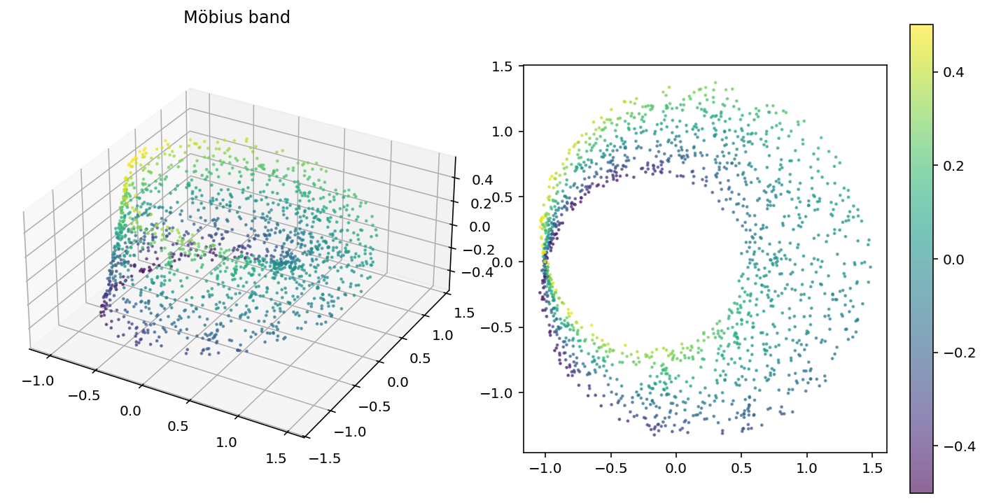
7.3 The Möbius band: non-orientable manifold with disconnected overlap

We apply our framework to the Möbius band, a fundamental example of a non-orientable surface. This experiment demonstrates that the sign cocycle detects non-orientability through the mechanism described in Remark 2.2: mixed signs on disconnected components of an overlap.

Data generation.

We sample $n=1500$ points from the Möbius band embedded in $\mathbb{R}^{3}$ using the standard parameterization (see Figure 5(a)).:

$$x(u,v)=\left(1+\frac{v}{2}\cos\frac{u}{2}\right)\cos u,\hskip 14.22636pty(u,v)=\left(1+\frac{v}{2}\cos\frac{u}{2}\right)\sin u,\hskip 14.22636ptz(u,v)=\frac{v}{2}\sin\frac{u}{2},$$

where $u\in[0,2\pi)$ and $v\in[-1,1]$. The half-angle terms create the characteristic twist: traversing the band once ($u:0\to 2\pi$) reverses the width direction ($v\mapsto-v$).

Cover construction.

We construct a simple two-chart cover by partitioning along the $y$-coordinate (see Figure 5(b)):

$$U_{0}=\{x\in M:y(x)>-0.3\},\qquad U_{1}=\{x\in M:y(x)<0.3\}.$$

Each chart domain is connected and contractible (a thickened arc along the band). The overlap $U_{0}\cap U_{1}=\{x:-0.3<y(x)<0.3\}$ consists of two disconnected components: one on each side of the band where $y\approx 0$. These two components are related by the Möbius twist, traversing the band from one component to the other reverses orientation.

This topological structure is essential for detecting non-orientability. By Remark 2.2, we treat each connected component of the overlap separately when computing the Čech cochains.

Results.

In Figures 5(c) and 5(d), the learned charts and the transition maps are shown.

Table 2: Theoretical metrics for Möbius band (mean $\pm$ std over 5 trials)

Metric	Value	Theoretical Role
$\varepsilon$	$0.098\pm 0.018$	$\sup_{x}\|D_{i}(E_{i}(x))-x\|$
$\eta_{lat}$	$0.47\pm 0.12$	$\sup_{x}\|d(E_{i}\circ D_{i})_{E_{i}(x)}-I_{d}\|_{\mathrm{op}}$
$\delta$	$0.36\pm 0.18$	$\min_{i,j,x}|\det g_{ji}(x)|$
$\sigma_{\min}(dE)$	$0.55\pm 0.09$	$\min\sigma_{\min}(dE_{i})$
Non-orientability detection: 100% (5/5 trials)
Detected via: opposite signs in disconnected overlap components

The necessary conditions $\delta>0$ and small $\varepsilon$ from Theorem 4.7 are satisfied. Verification of the full quantitative stability bound would additionally require estimating the Lipschitz constants.

1. The reconstruction error $\varepsilon\approx 0.098$ and deviation $\eta_{lat}<1$ validate the atlas.

2. The non-degeneracy gap $\delta\approx 0.36$ is bounded well away from zero, satisfying Theorem 4.7.

Detection mechanism: opposite signs in disconnected components.

The key to detecting non-orientability lies in the structure of the overlap $U_{0}\cap U_{1}$. This overlap consists of two connected components (the two regions where $y\approx 0$), related by the Möbius twist. We observe:

$$\omega_{10}|_{\text{Component 0}}=-1,\qquad\omega_{10}|_{\text{Component 1}}=+1.$$

For the sign cocycle to be a coboundary, we require orientations $\nu_{0},\nu_{1}\in\{\pm 1\}$, each constant on the connected charts $U_{0}$ and $U_{1}$, such that $\omega_{10}(x)=\nu_{1}\cdot\nu_{0}$ for all $x\in U_{0}\cap U_{1}$. This is impossible: Component 0 requires $\nu_{1}\cdot\nu_{0}=-1$, while Component 1 requires $\nu_{1}\cdot\nu_{0}=+1$, a contradiction since $\nu_{0}$ and $\nu_{1}$ must each be constant.

This is precisely the topological obstruction to orientability: the Möbius twist reverses orientation when traversing the band, and this is detected by the sign cocycle taking opposite values on the two sides of the twist.

Theoretical interpretation.

The coboundary condition in $\check{H}^{1}(\mathcal{U};\mathbb{Z}/2)$ requires finding a 0-cochain $\{\nu_{i}\}$ with $\delta^{0}\nu=\omega$, i.e., $\omega_{ji}=\nu_{j}\cdot\nu_{i}$. When an overlap has multiple components with different signs, no such 0-cochain exists.

By Proposition 3.15 and Corollary 4.14, this confirms $w_{1}(\mathcal{T}_{\mathcal{A}})\neq 0$, correctly detecting the non-orientability of the Möbius band.

(a) Sampled Möbius band in $\mathbb{R}^{3}$ with two-chart cover. Points are colored by chart assignment ($U_{0}$, $U_{1}$), with the overlap region $U_{0}\cap U_{1}$ highlighted.

(b) Chart domains and overlap decomposition. The overlap $U_{0}\cap U_{1}$ splits into two disconnected components, related by the Möbius twist.

(c) Latent representations $E_{0}(U_{0})$ and $E_{1}(U_{1})$ in $\mathbb{R}^{2}$.

(d) Transition map $T_{10}=E_{1}\circ D_{0}$ on the two overlap components, with $\mathrm{sign}(\det g_{10})$ indicated. Opposite signs confirm $[\omega]\neq 0\in\check{H}^{1}(\mathcal{U};\mathbb{Z}/2)$.

Figure 5: Autoencoder atlas for the Möbius band (Section 7.3). The two-chart cover produces an overlap with two disconnected components on which the sign cocycle takes opposite values ($\omega_{10}=-1$ and $\omega_{10}=+1$), detecting non-orientability via the failure of the coboundary condition.

Conclusion.

The 100% detection rate across trials demonstrates that our framework reliably identifies non-orientability through the mathematically correct mechanism: the failure of the coboundary condition due to mixed signs on disconnected overlap components.

7.4 Preliminary validation for the low-dimensional datasets

Table 3: Summary of experimental results

Manifold	$\varepsilon$	$\delta$	Ground Truth	Detection	Accuracy
$S^{2}$	0.033	0.10	Orientable	Orientable	100%
Möbius	0.098	0.36	Non-orientable	Non-orientable	100%

The experiments validate the theoretical framework:

1. Cocycle consistency from reconstruction (Lemma 3.8): Both experiments achieved cocycle errors $<0.03$ using reconstruction loss alone, confirming that explicit cocycle regularisation is unnecessary.

2. Sign stability (Theorem 4.7): The non-degeneracy gaps $\delta\in[0.10,0.36]$ ensured stable sign determination across all trials, with 100% consistency.

3. Correct classification (Corollary 4.14): The coboundary test correctly distinguished orientable ($S^{2}$) from non-orientable (Möbius) manifolds in all trials.

4. Disconnected overlap handling (Remark 2.2): The Möbius band experiment demonstrates correct treatment of disconnected overlap components, detecting non-orientability through opposite signs rather than a failing coboundary test on a connected overlap.

7.5 Higher-dimensional experiments: Klein bottle and $\mathbb{RP}^{2}$

We extend our experiments to more topologically complex manifolds: the Klein bottle (non-orientable, embedded in $\mathbb{R}^{4}$) and the real projective plane $\mathbb{RP}^{2}$ represented as a high-dimensional image dataset. These experiments test the framework on manifolds where covers must be learned from data, training convergence is not guaranteed, and the hypotheses of the stability theorems may not be fully satisfied.

On the importance of good covers.

The theoretical results of Sections 3.2 and 4 require the cover $\{U_{i}\}$ to be a good cover (Definition 2.1): each chart domain and every connected component of every finite intersection must be contractible. For $S^{2}$ and the Möbius band, we constructed covers with analytically verified contractibility. For the Klein bottle and $\mathbb{RP}^{2}$, the covers are learned from data via landmark-based geodesic balls, and we cannot analytically guarantee the good cover property.

Verifying contractibility of subsets from finite samples is a well-known difficult problem in computational topology; the recent work of Scoccola, Lim, and Harrington [15] identifies and studies this cover learning problem as an important challenge in its own right. In our experiments, we apply DBSCAN clustering (with threshold parameter $\varepsilon_{\mathrm{cluster}}$) to decompose each overlap region into connected components, and compute signs separately on each component. This decomposition provides a practical heuristic: small, connected, metrically concentrated subsets of a smooth manifold are generically contractible. However, we cannot formally guarantee the good cover property for these data-driven charts. We regard this as acceptable for two reasons: first, the theoretical framework degrades gracefully when the good cover condition is only approximately satisfied (Remark 2.2); second, the development of principled methods for learning covers with provable topological guarantees lies outside the scope of this paper.

Training convergence diagnostics.

A key practical insight from these experiments is that not all training runs produce valid atlases. We identify diagnostic criteria that reliably distinguish successful from unsuccessful training:

1. High reconstruction loss: High reconstruction loss indicates non-convergence of the training algorithm. Most of the times, this will also imply that the cocycle condition is not satisfied, and orientability detection is undefined.

2. Bounded differential error: The per-chart differential error is approximated by $\eta_{i}=\sup_{x}\|d(D_{i}\circ E_{i})_{x}-I\|_{\mathrm{op}}$ and should remain moderate across all charts. As the Klein bottle experiments below demonstrate, even a single chart with $\eta_{i}\gg 1$ can corrupt the global sign cocycle and produce incorrect results, even when sign consistency is satisfied.

These diagnostics allow us to identify, before examining orientability results, whether a given training run has produced a valid atlas structure.

7.5.1 Klein bottle

The Klein bottle is a compact, non-orientable 2-manifold that cannot be embedded in $\mathbb{R}^{3}$ without self-intersection. We sample $n=1000$ points from the standard immersion in $\mathbb{R}^{4}$ given by

$$\iota(u,v)=\bigl((m+\cos v)\cos u,\;(m+\cos v)\sin u,\;\sin v\cos(u/2),\;\sin v\sin(u/2)\bigr),$$

with $m=4$, $u\in[0,2\pi)$, $v\in[0,2\pi)$, and the identification $(u,v)\sim(u+2\pi,2\pi-v)$ encoding the non-orientable twist. Since $m>1$, $\iota$ descends to an injective immersion of the Klein bottle in $\mathbb{R}^{4}$.

Cover construction.

We construct an 8-chart cover using landmark-based geodesic balls. Geodesic distances are approximated via a $k$-nearest-neighbour graph ($k=100$), and 8 landmark points are selected by farthest-point sampling. Each chart $U_{i}$ consists of all sample points whose geodesic distance to landmark $i$ is below the 20th percentile of the landmark distance matrix. This yields chart sizes ranging from 139 to 327 points, with 17 pairwise overlaps and 11 triple overlaps.

Architecture and training.

Each chart autoencoder has an encoder and a decoder with hidden layers of widths $[32,16]$, latent dimension 2, and $\tanh$ activations throughout. Training uses Adam with learning rate $10^{-3}$ for 4000 epochs, batch size 64, and Jacobian regularisation $\lambda_{\mathrm{jac}}=0.01$. No cocycle regularisation is applied ($\lambda_{\mathrm{cocycle}}=0$). We employ a retry mechanism: if the maximum per-chart reconstruction error exceeds the threshold $\varepsilon_{\mathrm{thresh}}=0.15$ after initial training, the run is extended by 2000 additional epochs or restarted with a new seed, for up to 3 retries. Connected components of overlap regions are identified via DBSCAN with threshold $\varepsilon_{\mathrm{cluster}}=1.0$ and minimum cluster size 20.

Results.

We run 5 independent trials (seeds 42–46). Table 4 reports per-trial theoretical metrics and orientability detection results.

Table 4: Klein bottle: per-trial results over 5 independent runs. Metrics: $\varepsilon=\max_{i}\sup_{x}\|D_{i}(E_{i}(x))-x\|$, $\bar{\varepsilon}$ = mean reconstruction error (averaged over charts), $\eta=\max_{i}\sup_{x}\|d(D_{i}\circ E_{i})_{x}-I\|_{\mathrm{op}}$, $\delta=\min_{i,j,x}|\det g_{ji}(x)|$, $\sigma_{\min}(dE)=\min_{i}\sigma_{\min}(\nabla E_{i})$.

Trial	Seed	$\varepsilon$	$\bar{\varepsilon}$	$\eta_{lat}$	$\delta$	$\sigma_{\min}(dE)$	Detected	Correct
0	42	0.182	0.018	31.11	0.008	0.236	Orientable	✗
1	43	0.109	0.025	1.51	0.083	0.207	Non-orientable	✓
2	44	0.141	0.018	6.04	0.016	0.240	Orientable	✗
3	45	0.131	0.025	0.62	0.090	0.212	Non-orientable	✓
4	46	0.104	0.022	1.23	0.053	0.258	Non-orientable	✓

Overall accuracy is 60% (3/5 trials). Notably, all five trials achieve sign consistency within each overlap component (zero inconsistent pairs across all 13 overlap components), and the cocycle condition (Lemma 3.8) is verified across all 11 triple overlaps with cocycle error $\approx 0.012\pm 0.002$. This confirms that the $\mathbb{Z}/2$-valued sign cocycle $\omega_{ji}=\mathrm{sign}(\det g_{ji})$ is well-defined in every trial, regardless of detection outcome. The sign consistency diagnostic alone is therefore insufficient; the high values of the differential error $\eta$ and the small values of $\delta$ play a critical discriminating role.

Diagnostic analysis: the role of $\eta_{lat}$.

The two incorrect trials (seeds 42 and 44) share a distinctive pathology: a single chart, chart 4, the largest with 327 points, exhibits anomalously high differential error $\eta_{lat}$, while all other charts maintain $\eta_{lat}<1$:

Trial	$\eta$ (chart 4)	$\max_{i\neq 4}\,\eta_{i}$
0 (seed 42, ✗)	31.11	0.62
2 (seed 44, ✗)	6.04	0.67
1 (seed 43, ✓)	0.71	1.51
3 (seed 45, ✓)	0.60	0.62
4 (seed 46, ✓)	1.23	0.91

When $\eta_{lat,i}$ is large on a chart, the reconstruction map $D_{i}\circ E_{i}$ deviates substantially from the identity on tangent spaces, so the linearised transition maps $g_{ji}(x)=d(E_{j}\circ D_{i})_{E_{i}(x)}$ no longer approximate the true differential of the coordinate change. In particular, $\mathrm{sign}(\det g_{ji})$ may fail to reflect the true orientation relationship. The resulting sign cocycle, while well-defined and consistent, represents a different cohomology class from the true $w_{1}$, in these failed cases, a trivial class, causing the coboundary test to incorrectly pass.

The two incorrect trials also exhibit small non-degeneracy gaps ($\delta=0.008$ and $\delta=0.016$), an order of magnitude below the correct trials ($\delta\approx 0.076\pm 0.016$). The small $\delta$ arises because the outlier chart contributes transition maps whose Jacobian determinants pass near zero. While the signs remain individually consistent, the global sign pattern is distorted on all overlaps involving chart 4, destroying the non-trivial cohomology class.

This analysis identifies the per-chart differential error $\eta_{lat,i}$ and the non-degeneracy gap $\delta$ as the critical diagnostics for atlas validity, consistent with the theoretical framework of Theorem 4.7.

Converged trials.

Restricting to the three correct trials (seeds 43, 45, 46), we obtain:

Table 5: Klein bottle: summary metrics for converged trials (mean $\pm$ std over 3 trials).

Metric	Value
$\varepsilon$ (sup reconstruction error)	$0.115\pm 0.012$
$\bar{\varepsilon}$ (mean reconstruction error)	$0.024\pm 0.001$
$\eta_{lat}$ (differential error)	$1.12\pm 0.46$
$\delta$ (non-degeneracy gap)	$0.076\pm 0.016$
Cocycle error	$0.013\pm 0.001$
$\sigma_{\min}(dE)$ (encoder regularity)	$0.226\pm 0.023$

In all three converged trials, the coboundary test correctly fails: the sign cocycle $\omega$ admits no $\mathbb{Z}/2$-valued 0-cochain $\{\nu_{i}\}$ satisfying $\omega_{ji}=\nu_{j}\cdot\nu_{i}$, confirming $[\omega]\neq 0\in\check{H}^{1}(\mathcal{U};\mathbb{Z}/2)$ and hence $w_{1}(\mathcal{T}_{\mathcal{A}})\neq 0$. The sign distributions across the 13 overlap components are:

• Trial 1 (seed 43): 5 positive, 8 negative;

• Trial 3 (seed 45): 8 positive, 5 negative;

• Trial 4 (seed 46): 7 positive, 6 negative.

The balanced sign distributions, with no consistent 2-colouring of the overlap graph, correctly identify the Klein bottle as non-orientable.

Relationship to the stability theorem.

The converged trials have $\eta_{lat}\approx 1.12$. The non-degeneracy gap $\delta\approx 0.076>0$ does satisfy the positivity requirement, and the cocycle errors are small ($\approx 0.013$), indicating good transition map consistency.

The sign cocycle correctly detects non-orientability with $\eta_{\mathrm{lat}}\approx 1.12$ which indicates that the practical diagnostic need not satisfy the formal bound $\eta<1$ of Theorem 4.7 for detection to succeed. The condition $\eta<1$ in the theorem serves two purposes: it ensures $\delta>0$ a priori (Proposition 3.15), and it contributes to the perturbation bound $\Gamma<\delta$ needed for sign agreement (Theorem 4.10). When $\delta>0$ is verified directly from the data, the first purpose is unnecessary. For the second, the bound $\Gamma<\delta$ can still hold even when the $\eta$-dependent terms are large, provided $\delta$ is sufficiently large to absorb them. In our converged Klein bottle trials, $\delta\approx 0.21$ remains well-separated from zero despite $\eta_{\mathrm{lat}}\approx 1.12$, consistent with this interpretation.

7.5.2 $\mathbb{RP}^{2}$ via line patches

This experiment tests our framework on genuinely high-dimensional data. We generate 5625 line patch images (ambient dimension 100) following the construction in [12]: each image is a $10\times 10$ grayscale patch containing a blurred line segment. Since a line at angle $\theta$ is identical to a line at angle $\theta+\pi$, and the persistent cohomology of this space has been shown to be consistent with $\mathbb{RP}^{2}$ [12], this provides a natural high-dimensional test case for orientability detection of non-orientable manifolds.

We use a 10-chart cover derived from projective landmarks with no Jacobian regularisation ($\lambda_{\mathrm{jac}}=0$), $\tanh$ activations, and 1000 training epochs, testing whether the framework succeeds on high-dimensional data without explicit regularisation.

Results.

Of five training runs, four satisfied the convergence criteria (trials with seeds 43, 44, 45, 46). In all four cases, the coboundary test correctly failed, detecting non-orientability:

• Trial 1 (seed 43): 11 positive signs, 14 negative signs across 25 overlaps;

• Trial 2 (seed 44): 16 positive signs, 9 negative signs across 25 overlaps;

• Trial 3 (seed 45): 12 positive signs, 13 negative signs across 25 overlaps;

• Trial 4 (seed 46): 15 positive signs, 10 negative signs across 25 overlaps.

In each of these trials, $\delta>0$, no overlap component exhibited mixed signs, and the $\check{C}^{1}$ sign assignment was verified as a cocycle while failing to be a coboundary. The balanced (though not perfectly symmetric) sign distributions confirm that the nerve graph admits no consistent 2-colouring, correctly detecting $w_{1}(\mathcal{T}_{\mathcal{A}})\neq 0$.

Figure 6 visualises the learned transition maps across all pairwise overlaps; the mix of orientation-preserving and orientation-reversing transitions confirms the non-trivial sign cocycle.

Table 6: $\mathbb{RP}^{2}$ line patches: summary metrics for converged trials (mean $\pm$ std over 4 trials).

Metric	Value
$\varepsilon$ (sup reconstruction error)	$0.309\pm 0.081$
$\bar{\varepsilon}$ (mean reconstruction error)	$0.060\pm 0.003$
$\eta$ (differential error)	$12.90\pm 6.91$
$\delta$ (non-degeneracy gap)	$0.027\pm 0.010$
Cocycle error	$0.042\pm 0.008$
$\sigma_{\min}(dE)$ (encoder regularity)	$0.541\pm 0.064$

Relationship to the stability theorem.

The $\mathbb{RP}^{2}$ experiments exhibit $\eta_{lat}\gg 1$ in all trials (with maxima ranging from approximately $4.07$ up to $24.75$), placing them well outside the regime of Theorem 4.7. As with the Klein bottle, the correct detection is therefore an empirical observation: the sign cocycle correctly captures the non-trivial $w_{1}$ even when the formal hypotheses of the stability theorem are not satisfied, provided that $\delta>0$ and sign consistency hold.

The role of Jacobian regularisation.

Ablation experiments without Jacobian regularisation ($\lambda_{\mathrm{jac}}=0$) on the Klein bottle resulted in 0% accuracy: all five trials did not satisfy the convergence criteria. In contrast, $\mathbb{RP}^{2}$ achieved convergence on 4 out of 5 trials. This confirms that the regularisation term is beneficial but not universally necessary; its importance depends on the cover structure and data geometry.

7.6 Summary and discussion

Table 7 summarises the results across all manifolds, reporting accuracy only for trials that satisfy the convergence diagnostics (sign consistency within overlaps, moderate per-chart $\eta$, and $\delta>0$).

Table 7: Summary of experimental results (converged trials only). Here $\bar{\varepsilon}$ denotes the mean reconstruction error (averaged over charts and converged trials), and $\delta$ denotes the mean non-degeneracy gap over converged trials.

Manifold	Dim	Ambient	Ground Truth	$\bar{\varepsilon}$	$\delta$	Converged	Accuracy
$S^{2}$	2	$\mathbb{R}^{3}$	Orientable	0.032	0.10	5/5	100%
Möbius band	2	$\mathbb{R}^{3}$	Non-orientable	0.098	0.36	5/5	100%
Klein bottle	2	$\mathbb{R}^{4}$	Non-orientable	0.024	0.076	3/5	100%
$\mathbb{RP}^{2}$ (patches)	2	$\mathbb{R}^{100}$	Non-orientable	0.060	0.042	4/5	100%

The experimental validation demonstrates four key findings:

1. Theoretical correctness: When the atlas diagnostics are satisfied, orientability detection achieves 100% accuracy across all tested manifolds, including high-dimensional image data. This confirms the mathematical soundness of computing $w_{1}(\mathcal{T}_{\mathcal{A}})$ via the sign cocycle coboundary test (Corollary 4.14).

2. Cocycle consistency from reconstruction: All converged trials achieved cocycle errors below 0.08 using reconstruction loss alone, with no explicit cocycle regularisation term ($\lambda_{\mathrm{cocycle}}=0$). This validates Lemma 3.8: the encoding consistency condition $E_{j}(D_{i}(E_{i}(x)))\approx E_{j}(x)$ emerges automatically from minimizing reconstruction error.

3. Practical diagnostics: The diagnostic criteria, moderate per-chart differential error $\eta_{i}$, and positive non-degeneracy gap $\delta$, provide a reliable method for determining whether a given training run has produced a valid atlas, without requiring knowledge of the ground truth orientability. The Klein bottle experiment demonstrates that sign consistency alone is insufficient: $\eta$ and $\delta$ are essential complementary diagnostics. This enables practical deployment: one first verifies atlas validity, then applies the coboundary test only to valid atlases.

4. Scalability to high dimensions: The $\mathbb{RP}^{2}$ experiment demonstrates that the framework scales to genuinely high-dimensional ambient spaces ($\mathbb{R}^{100}$) while correctly detecting topological properties of the underlying 2-dimensional manifold. This validates the approach for real-world image and signal data where the ambient dimension far exceeds the intrinsic dimension.

The varying convergence rates across manifolds reflect differences in optimisation difficulty rather than theoretical limitations. The simpler manifolds ($S^{2}$, Möbius band) with carefully constructed covers achieve 100% convergence, while more complex manifolds with automatically generated covers show lower rates. This suggests that cover construction and training methodology are important practical considerations for future work.

On the hypotheses of the stability theorem.

The Klein bottle and $\mathbb{RP}^{2}$ experiments reveal a gap between the sufficient conditions of Theorem 4.7 and practical detection. The theorem requires $\eta<1$, yet the Klein bottle converged trials achieve correct detection with $\eta_{lat}\approx 1.12$, and the $\mathbb{RP}^{2}$ trials succeed with $\eta_{lat}\gg 1$. Meanwhile, Klein bottle trials with $\eta_{lat}\gg 1$ (driven by a single outlier chart) fail. This suggests that the operationally relevant condition is not a uniform bound $\eta_{lat}<1$ across all charts, but rather that $\eta_{lat}$ remains moderate on charts participating in the overlap graph cycles that carry the non-trivial cohomology class. A single chart with extreme $\eta_{lat}$ can corrupt the sign cocycle on all its incident overlaps, potentially trivialising a non-trivial class. Formalising this local condition and tightening the stability bounds accordingly is an important direction for future work; the experiments suggest that the sufficient conditions of Theorem 4.7 can be substantially relaxed when $\delta>0$ is verified directly.

Computational considerations.

The Jacobian computation $g_{ji}(x)=d(T_{ji})_{E_{i}(x)}$ requires automatic differentiation through the encoder-decoder composition. For neural networks with smooth activations ($\tanh$), this is well-conditioned even in high ambient dimensions. The coboundary test reduces to checking whether the nerve graph admits a consistent 2-colouring, solvable in linear time. The overall computational cost is dominated by autoencoder training, which scales with the number of charts, dataset size, and ambient dimension.

8 Conclusions and future work

We have introduced a framework that treats collections of locally trained autoencoders as learned atlases on data manifolds, connecting neural network representations to the classical theory of vector bundles and characteristic classes. The key theoretical insight is that reconstruction consistency alone enforces the cocycle condition on transition maps, and that linearising these transitions yields a vector bundle whose first Stiefel–Whitney class can be read off from the signs of Jacobian determinants. We proved stability of this sign cocycle under approximate reconstruction (Theorem 4.7) and its agreement with $w_{1}(TM)$ when the learned atlas is close to an exact compatible atlas (Theorem 4.10). We also showed that the minimum number of autoencoder charts over good covers equals the covering type of the manifold (Corollary 5.8).

Experiments on the 2-sphere, Möbius band, Klein bottle, and $\mathbb{RP}^{2}$ line patches in $\mathbb{R}^{100}$ validate the framework: converged trials achieve 100% orientability detection accuracy using reconstruction loss alone, with no explicit cocycle regularisation. The experiments also reveal that the sufficient conditions of the stability theorem are not tight, and correct detection occurs even when the formal bound $\eta<1$ is violated, provided the non-degeneracy gap $\delta$ remains positive, and the per-chart differential error remains moderate.

Several directions for future work arise naturally. The linearised transition functions $g_{ji}(x)\in\mathrm{GL}(d,\mathbb{R})$ carry more information than their $\mathbb{Z}/2$ sign cocycle; extracting higher Stiefel–Whitney classes, or Chern classes in the complex setting, would detect finer topological obstructions. The stability theory could be tightened by replacing the global bound on $\eta$ with local conditions on charts participating in cohomology-carrying cycles. Integrating principled cover learning methods [15] with our framework would close the gap between the theoretical requirement of a good cover and the data-driven covers used in practice. Finally, scaling the approach to higher intrinsic dimensions and applying it to domains where characteristic classes carry practical significance, such as robotics, computer vision, or materials science, remains an important open direction.

Code availability

The code is available at https://github.com/EduPH/learningtangentbundle.

Appendix A Proofs of Section 4

Proof of Theorem 4.7.

Fix $x\in U_{i}\cap U_{j}\cap U_{k}$ and set $y\coloneqq D_{i}(E_{i}(x))$. By Proposition 4.3, the sign $\omega_{ji}$ is constant on each connected component of each overlap. It suffices to show that

$$\mathrm{sign}(\det g_{ki}(x))=\mathrm{sign}(\det(g_{kj}(y)\cdot g_{ji}(x))).$$

We establish this by showing that $|\det g_{ki}(x)-\det(g_{kj}(y)\cdot g_{ji}(x))|$ is strictly less than $|\det g_{ki}(x)|$, which forces both determinants to have the same sign.

Step 0: Domain verification. Since $x\in U_{i}\cap U_{j}\cap U_{k}$ and $\|y-x\|=\|D_{i}(E_{i}(x))-x\|\leq\varepsilon$, the point $y$ lies in $O_{j}\cap O_{k}$ by Definition 4.1(5). In particular, the encoders $E_{j}$ and $E_{k}$ are $C^{1}$ at $y$, so the Jacobians $g_{kj}(y)=d(T_{kj})_{E_{j}(y)}$ and $g_{ji}(x)=d(T_{ji})_{E_{i}(x)}$ are both well-defined. Moreover, the reconstruction map $\Phi_{j}=D_{j}\circ E_{j}$ is $C^{1}$ at $y$ since $y\in O_{j}$, and $\Phi_{j}(y)$ lies in $O_{k}$ by Remark 4.5.

Step 1: Bounding the Jacobian perturbation. By Lemma 4.4, we can write

$$g_{ki}(x)=Q\cdot P,\qquad g_{kj}(y)\cdot g_{ji}(x)=Q^{\prime}RP,$$

where

$$P\coloneqq d(D_{i})_{E_{i}(x)}\in\mathbb{R}^{N\times d},\quad Q\coloneqq d(E_{k})_{y}\in\mathbb{R}^{d\times N},\quad Q^{\prime}\coloneqq d(E_{k})_{\Phi_{j}(y)}\in\mathbb{R}^{d\times N},\quad R\coloneqq d(\Phi_{j})_{y}\in\mathbb{R}^{N\times N}.$$

That is, the direct transition Jacobian $g_{ki}(x)$ factors as encoder-times-decoder through the ambient space $\mathbb{R}^{N}$, while the composed transition Jacobian additionally inserts the reconstruction map $\Phi_{j}=D_{j}\circ E_{j}$ and evaluates the encoder $E_{k}$ at the shifted point $\Phi_{j}(y)$ instead of $y$.

We write $Q^{\prime}=Q+\Delta_{Q}$ and $\Delta_{R}\coloneqq R-I_{N}$, so that

$$Q^{\prime}RP=QP+\underbrace{Q\,\Delta_{R}\,P+\Delta_{Q}\,(I_{N}+\Delta_{R})\,P}_{=:\,\Delta}.$$ (7)

Thus $g_{kj}(y)\cdot g_{ji}(x)=g_{ki}(x)+\Delta$, and it remains to bound $\|\Delta\|_{\mathrm{op}}$.

Step 1a: The restricted action of $\Delta_{R}$ on $\mathrm{range}(P)$. A naïve bound on $\|Q\,\Delta_{R}\,P\|_{\mathrm{op}}$ using the full operator norm $\|\Delta_{R}\|_{\mathrm{op}}$ fails: since $\Phi_{j}=D_{j}\circ E_{j}$ factors through $\mathbb{R}^{d}$, the differential $R=d(\Phi_{j})_{y}$ has rank at most $d<N$ and therefore annihilates a subspace of dimension at least $N-d$. This forces $\|\Delta_{R}\|_{\mathrm{op}}=\|R-I_{N}\|_{\mathrm{op}}\geq 1$ regardless of the quality of the reconstruction.

The key observation is that only the restricted action of $\Delta_{R}$ on $\mathrm{range}(P)$ enters the product $Q\,\Delta_{R}\,P$. We now show that vectors in $\mathrm{range}(P)$ are nearly tangent to $M$, which allows us to exploit the approximate reconstruction condition on tangent directions.

Fix a unit vector $v\in\mathbb{R}^{d}$ and set $w\coloneqq Pv=d(D_{i})_{E_{i}(x)}\,v$. The differential reconstruction condition (Definition 4.1(4)) for chart $i$ states that $d(\Phi_{i})_{x}|_{T_{x}M}$ is within operator-norm distance $\eta$ of $\mathrm{Id}_{T_{x}M}$. Since $\eta<1$, the restricted map $d(\Phi_{i})_{x}|_{T_{x}M}=P\circ d(E_{i})_{x}|_{T_{x}M}$ is invertible. In particular, $d(E_{i})_{x}|_{T_{x}M}\colon T_{x}M\to\mathbb{R}^{d}$ is a bijection, so there exists a unique $u\in T_{x}M$ satisfying $d(E_{i})_{x}\,u=v$. Then

$$w=P\,v=d(D_{i})_{E_{i}(x)}\,d(E_{i})_{x}\,u=d(\Phi_{i})_{x}\,u,$$

and condition (4) gives $\|w-u\|\leq\eta\,\|u\|$.

Since $u\in T_{x}M$, we can decompose $w=w_{T}+w_{\perp}$ with $w_{T}\in T_{x}M$ and $w_{\perp}\perp T_{x}M$. The normal component is controlled by:

$$\|w_{\perp}\|=\|\Pi_{T_{x}M}^{\perp}(w-u)\|\leq\|w-u\|\leq\eta\,\|u\|\leq\frac{\eta}{1-\eta}\,\|w\|,$$ (8)

where the last step uses $\|w\|\geq\|u\|-\|w-u\|\geq(1-\eta)\|u\|$.

Step 1b: Bounding $\|\Delta_{R}\,w\|$ via the tangent–normal decomposition. We bound $\|\Delta_{R}\,w\|=\|[d(\Phi_{j})_{y}-I_{N}]\,w\|$ by treating the tangential and normal parts of $w$ separately.

Tangential component. Since $x\in U_{j}$ and $w_{T}\in T_{x}M$, condition (4) for chart $j$ gives $\|[d(\Phi_{j})_{x}-I_{N}]\,w_{T}\|\leq\eta\,\|w_{T}\|$. To pass from the on-manifold point $x$ to the off-manifold point $y$, we use the derivative Lipschitz constant $L_{\Phi}^{\prime}\coloneqq L_{D}^{\prime}L_{E}^{2}+L_{D}L_{E}^{\prime}$ of $p\mapsto d(\Phi_{j})_{p}$ on $O_{j}$ (see Remark 4.9). Since $\|y-x\|\leq\varepsilon$:

$$\|[d(\Phi_{j})_{y}-I_{N}]\,w_{T}\|\leq\|[d(\Phi_{j})_{x}-I_{N}]\,w_{T}\|+\|d(\Phi_{j})_{y}-d(\Phi_{j})_{x}\|_{\mathrm{op}}\,\|w_{T}\|\leq(\eta+L_{\Phi}^{\prime}\,\varepsilon)\,\|w_{T}\|\leq(\eta+L_{\Phi}^{\prime}\,\varepsilon)\,\|w\|.$$

Normal component. For the normal part, no reconstruction guarantee is available—the reconstruction map $\Phi_{j}$ has no reason to act as the identity on directions normal to $M$. We therefore use the crude bound $\|d(\Phi_{j})_{y}\|_{\mathrm{op}}\leq L_{E}L_{D}$:

$$\|[d(\Phi_{j})_{y}-I_{N}]\,w_{\perp}\|\leq(\|d(\Phi_{j})_{y}\|_{\mathrm{op}}+1)\,\|w_{\perp}\|\leq(L_{E}L_{D}+1)\,\|w_{\perp}\|\leq\frac{(L_{E}L_{D}+1)\,\eta}{1-\eta}\,\|w\|,$$

where the last step uses (8). This is the normal-direction amplification: the factor $(L_{E}L_{D}+1)$ multiplies the normal component, which is itself of relative size $\eta/(1-\eta)$.

Combining. Adding the two contributions and simplifying,

$$\|\Delta_{R}\,w\|\leq\biggl(\eta+L_{\Phi}^{\prime}\varepsilon+\frac{(L_{E}L_{D}+1)\eta}{1-\eta}\biggr)\|w\|\leq\underbrace{\biggl(\frac{(L_{E}L_{D}+2)\eta}{1-\eta}+L_{\Phi}^{\prime}\varepsilon\biggr)}_{=:\,\eta_{\mathrm{eff}}}\|w\|,$$ (9)

where the simplification uses $\eta+\frac{(L_{E}L_{D}+1)\eta}{1-\eta}\leq\frac{(L_{E}L_{D}+2)\eta}{1-\eta}$. Since $w=Pv$ and $\|w\|\leq L_{D}\|v\|$, we obtain

$$\|\Delta_{R}\,P\,v\|\leq\eta_{\mathrm{eff}}\,L_{D}\,\|v\|\qquad\text{for every }v\in\mathbb{R}^{d}.$$ (10)

Step 1c: Bounding $\|\Delta_{Q}\|_{\mathrm{op}}$. The matrices $Q=d(E_{k})_{y}$ and $Q^{\prime}=d(E_{k})_{\Phi_{j}(y)}$ differ because the encoder $E_{k}$ is evaluated at the shifted point $\Phi_{j}(y)$ rather than $y$. By the encoder derivative Lipschitz condition (ii) and Lemma 4.6:

$$\|\Delta_{Q}\|_{\mathrm{op}}=\|d(E_{k})_{\Phi_{j}(y)}-d(E_{k})_{y}\|_{\mathrm{op}}\leq L_{E}^{\prime}\,\|\Phi_{j}(y)-y\|\leq L_{E}^{\prime}\,\widetilde{\varepsilon},$$ (11)

where $\widetilde{\varepsilon}\coloneqq(L_{E}L_{D}+2)\varepsilon$ is the off-manifold reconstruction bound.

Step 1d: Assembling the bound on $\|\Delta\|_{\mathrm{op}}$. Returning to the decomposition $\Delta=Q\,\Delta_{R}\,P+\Delta_{Q}\,(I_{N}+\Delta_{R})\,P$ from (7), we bound each term separately.

For the first term, using (10):

$$\|Q\,\Delta_{R}\,P\|_{\mathrm{op}}\leq\|Q\|_{\mathrm{op}}\cdot\eta_{\mathrm{eff}}\,L_{D}\leq L_{E}\,\eta_{\mathrm{eff}}\,L_{D}.$$

For the second term, note that $\|(I_{N}+\Delta_{R})\,P\,v\|\leq\|P\,v\|+\|\Delta_{R}\,P\,v\|\leq(1+\eta_{\mathrm{eff}})\,L_{D}\,\|v\|$ by (10). Combined with (11):

$$\|\Delta_{Q}\,(I_{N}+\Delta_{R})\,P\|_{\mathrm{op}}\leq L_{E}^{\prime}\,\widetilde{\varepsilon}\,(1+\eta_{\mathrm{eff}})\,L_{D}.$$

Therefore:

$$\|\Delta\|_{\mathrm{op}}\leq\underbrace{L_{E}\,\eta_{\mathrm{eff}}\,L_{D}}_{\begin{subarray}{c}\text{reconstruction map}\\ \text{derivative error}\end{subarray}}\;+\;\underbrace{L_{E}^{\prime}\,\widetilde{\varepsilon}\,(1+\eta_{\mathrm{eff}})\,L_{D}}_{\begin{subarray}{c}\text{encoder evaluation}\\ \text{point shift}\end{subarray}}\;=\;\Gamma.$$ (12)

Step 2: Bounding the determinant perturbation. We have $g_{kj}(y)\cdot g_{ji}(x)=g_{ki}(x)+\Delta$ where $\Delta\in\mathbb{R}^{d\times d}$. By the multilinearity of the determinant in columns, for any $A,B\in\mathbb{R}^{d\times d}$, the telescoping identity

$$\det(A+B)-\det(A)=\sum_{l=1}^{d}\det\bigl[a_{1}\mid\cdots\mid a_{l-1}\mid b_{l}\mid(a_{l+1}+b_{l+1})\mid\cdots\mid(a_{d}+b_{d})\bigr]$$

(where $a_{l}$, $b_{l}$ denote the $l$-th columns of $A$, $B$) together with Hadamard’s inequality [8, Theorem 3.3.16] yields:

$$|\det(A+B)-\det(A)|\leq d\cdot\|B\|_{\mathrm{op}}\cdot(\|A\|_{\mathrm{op}}+\|B\|_{\mathrm{op}})^{d-1}.$$ (13)

Applying Equation (13) with $A=g_{ki}(x)$ and $B=\Delta$, and noting $\|A\|_{\mathrm{op}}\leq L_{E}L_{D}$ and $\|B\|_{\mathrm{op}}\leq\Gamma$:

$$|\det(g_{kj}(y)\cdot g_{ji}(x))-\det g_{ki}(x)|\leq d\cdot\Gamma\cdot(L_{E}L_{D}+\Gamma)^{d-1}.$$ (14)

Step 3: Sign agreement. By the non-degeneracy hypothesis, $|\det g_{ki}(x)|\geq\delta$. Equation (4) states that $d\cdot\Gamma\cdot(L_{E}L_{D}+\Gamma)^{d-1}<\delta$, so the right-hand side of (14) is strictly less than $|\det g_{ki}(x)|$. This forces $\det(g_{kj}(y)\cdot g_{ji}(x))$ to have the same sign as $\det g_{ki}(x)$:

$$\mathrm{sign}(\det g_{ki}(x))=\mathrm{sign}(\det(g_{kj}(y)\cdot g_{ji}(x)))=\mathrm{sign}(\det g_{kj}(y))\cdot\mathrm{sign}(\det g_{ji}(x)).$$

Step 4: Evaluation point correction. It remains to show that $\mathrm{sign}(\det g_{kj}(y))=\omega_{kj}(x)$. By Step 0, both $x$ and $y$ lie in $O_{j}\cap O_{k}$, and $\|y-x\|\leq\varepsilon$. Consider the line segment $\gamma(t)\coloneqq(1-t)x+ty$ for $t\in[0,1]$. Since $\|\gamma(t)-x\|\leq\varepsilon$ for all $t\in[0,1]$, and $\varepsilon$ is less than the tubular radius of $M\subset\mathbb{R}^{N}$ (guaranteed for $\varepsilon$ sufficiently small relative to the geometry of $M$), each $\gamma(t)\in O_{j}\cap O_{k}$. The function

$$t\mapsto\det g_{kj}(\gamma(t))=\det\bigl(d(E_{k})_{D_{j}(E_{j}(\gamma(t)))}\cdot d(D_{j})_{E_{j}(\gamma(t))}\bigr)$$

is continuous in $t$ (since all maps involved are $C^{1}$ on the relevant domains). The map $p\mapsto\det g_{kj}(p)$ has Lipschitz constant bounded by $L_{\det}\coloneqq d\,(L_{E}L_{D})^{d-1}\,L_{E}\,(L_{E}L_{D}^{\prime}+L_{E}^{\prime}L_{D}^{2})$ on $O_{j}\cap O_{k}$ (by differentiating the determinant of the product $d(E_{k})_{D_{j}(E_{j}(p))}\cdot d(D_{j})_{E_{j}(p)}$ via the chain rule and Hadamard’s inequality). Since $|\det g_{kj}(x)|\geq\delta$ and $\|\gamma(t)-x\|\leq\varepsilon$:

$$|\det g_{kj}(\gamma(t))|\geq\delta-L_{\det}\,\varepsilon>0,$$

which holds since $L_{\det}\,\varepsilon<\delta$ by Equation (4). Since the determinant is continuous and never vanishes along $\gamma$, the sign is constant:

$$\mathrm{sign}(\det g_{kj}(y))=\mathrm{sign}(\det g_{kj}(x))=\omega_{kj}(x).$$

Hence $\omega_{ki}(x)=\omega_{kj}(x)\cdot\omega_{ji}(x)$, as required. ∎

Remark A.1.

On the Step 4, the non-degeneracy of $\det g_{kj}(\gamma(t))$ along the segment from $x$ to $y$ follows from the continuity of $p\mapsto\det g_{kj}(p)$ and the explicit Lipschitz constant $L_{\det}$ defined in Equation (3). The condition $L_{\det}\,\varepsilon<\delta$ appears as the second branch of the maximum in Equation (4), ensuring that it is verified alongside the determinant perturbation bound. Neither condition implies the other: the first branch controls the cocycle defect (mixing $\eta$ and $\varepsilon$ through $\Gamma$), while the second controls the evaluation-point shift (depending on $\varepsilon$ alone).

Remark A.2.

In the exact setting ($\varepsilon=\eta=0$), the reconstruction map $\Phi_{j}$ is the identity on $M$, and the differential $d(\Phi_{j})_{x}$ acts as the identity on $T_{x}M$ while annihilating normal directions. The cocycle condition holds exactly because all relevant vectors lie in tangent spaces. However, in the approximate setting, the decoder differential $P=d(D_{i})_{E_{i}(x)}$ produces vectors $w=Pv$ that are nearly tangential but have a small normal component of size $O(\eta/(1-\eta))$ relative to $\|w\|$ (see Equation (8)). The reconstruction differential $d(\Phi_{j})_{y}-I_{N}$ acts well on the tangential part (controlled by $\eta+O(\varepsilon)$) but amplifies the normal part by up to $(L_{E}L_{D}+1)$. The effective error $\eta_{\mathrm{eff}}$ accounts for this amplification: it equals the tangent-restricted error $\eta$ plus a correction of order $(L_{E}L_{D})\eta/(1-\eta)$ from the normal component, plus an off-manifold evaluation correction of order $L_{\Phi}^{\prime}\varepsilon$.

Proof of Theorem 4.10.

Since $\|E_{i}-E_{i}^{0}\|_{C^{1}(U_{i})}\leq\mu$, the latent domains $Z_{i}=E_{i}(U_{i})$ and $Z_{i}^{0}=E_{i}^{0}(U_{i})$ satisfy $d_{H}(Z_{i},Z_{i}^{0})\leq\mu$ (in the $C^{0}$ sense), where $d_{H}$ denotes the Hausdorff distance. For $\mu$ sufficiently small, both $D_{i}^{0}$ and $D_{i}$ (being $C^{1}$ on their respective domains) extend as $C^{1}$ maps to a common open set $\widetilde{Z}_{i}\supset Z_{i}^{0}\cup Z_{i}$ in $\mathbb{R}^{d}$. (For $D_{i}^{0}=(E_{i}^{0})^{-1}$, this extension exists by the inverse function theorem, since $E_{i}^{0}$ is a diffeomorphism onto $Z_{i}^{0}$ and hence has non-degenerate Jacobian; for $D_{i}$, it is defined on $Z_{i}$ and extends by $C^{1}$ regularity.) We choose $\widetilde{Z}_{i}$ to be the open $\mu$-neighborhood of $Z_{i}^{0}$ in $\mathbb{R}^{d}$:

$$\widetilde{Z}_{i}\coloneqq\{z\in\mathbb{R}^{d}\colon\mathrm{dist}(z,Z_{i}^{0})<\mu\}.$$

Since $d_{H}(Z_{i},Z_{i}^{0})\leq\mu$, this ensures $Z_{i}\subset\widetilde{Z}_{i}$.

We define the interpolated atlas $\mathcal{A}_{t}=\{(U_{i},E_{i}^{t},D_{i}^{t})\}$ for $t\in[0,1]$ by

$$E_{i}^{t}\coloneqq(1-t)E_{i}^{0}+tE_{i},\qquad D_{i}^{t}\coloneqq(1-t)D_{i}^{0}+tD_{i},$$

where $D_{i}^{t}$ is well-defined on $\widetilde{Z}_{i}$. For any $x\in U_{i}$, the $C^{0}$ bound gives:

$$\|E_{i}^{t}(x)-E_{i}^{0}(x)\|=t\|E_{i}(x)-E_{i}^{0}(x)\|\leq t\mu\leq\mu,$$

so $E_{i}^{t}(x)\in B(E_{i}^{0}(x),\mu)\subset\widetilde{Z}_{i}$, confirming that $E_{i}^{t}(U_{i})\subset\widetilde{Z}_{i}$ for all $t\in[0,1]$.

Domain of the transition maps. The transition maps $T_{ji}^{t}=E_{j}^{t}\circ D_{i}^{t}$ require evaluating $E_{j}^{t}$ at points of the form $D_{i}^{t}(z)$ for $z\in E_{i}^{t}(U_{i})\subset\widetilde{Z}_{i}$. In the exact atlas, $D_{i}^{0}(E_{i}^{0}(x))=x\in M$. For the interpolated atlas, $D_{i}^{t}(E_{i}^{t}(x))$ is a convex combination of points within $O(\mu+\varepsilon)$ of $x$, and thus remains within $O(\mu+\varepsilon)$ of $M$. Since the encoders $E_{j}^{t}$ are defined on the extended neighborhoods $O_{j}$ (which contain a tubular neighborhood of $U_{j}$ of width $\varepsilon\geq O(\mu)$ for $\mu$ sufficiently small), the composition $T_{ji}^{t}$ and its Jacobians $g_{ji}^{t}(x)=d(T_{ji}^{t})_{E_{i}^{t}(x)}$ are well-defined and vary continuously in $t$.

Step 1: Uniform non-degeneracy along the homotopy. At $t=0$, the exact atlas has $|\det g_{ji}^{0}(x)|\geq\delta_{0}>0$ for all relevant $(i,j,x)$. Since $M$ is compact, each closure $\overline{U_{i}\cap U_{j}}$ is compact, and the maps $E_{i}^{t}$, $D_{i}^{t}$ are $C^{1}$ on neighborhoods of these closures. The function $(t,x)\mapsto\det g_{ji}^{t}(x)$ is therefore continuous on the compact set $[0,1]\times\overline{U_{i}\cap U_{j}}$ for each pair $(i,j)$, hence uniformly continuous. Taking the minimum over the finitely many pairs $(i,j)$, for $\mu$ satisfying Equation (5):

$$|\det g_{ji}^{t}(x)|\geq\frac{\delta_{0}}{2}>0\qquad\text{for all }t\in[0,1],\;x\in U_{i}\cap U_{j}.$$

Step 2: Sign constancy along the path. Since $\det g_{ji}^{t}(x)$ is continuous in $t$ and never vanishes, $\mathrm{sign}(\det g_{ji}^{t}(x))$ is constant in $t$ for each fixed $(i,j)$ and each connected component of $U_{i}\cap U_{j}$. Therefore $\omega_{ji}^{t}$ is independent of $t$:

$$\omega_{ji}^{1}=\omega_{ji}^{0}\qquad\text{on each connected component of }U_{i}\cap U_{j}.$$

Step 3: Conclusion. Since $\omega_{ji}^{\mathcal{A}}=\omega_{ji}^{1}=\omega_{ji}^{0}=\omega_{ji}^{\mathcal{A}_{0}}$, the two sign cocycles are identical (not merely cohomologous). By Proposition 3.13, $[\omega^{\mathcal{A}_{0}}]=w_{1}(\mathcal{T}_{\mathcal{A}_{0}})=w_{1}(TM)$, so $[\omega^{\mathcal{A}}]=w_{1}(TM)$. ∎

Figure 6: Transition maps $z\mapsto T_{ji}(z)=E_{j}(D_{i}(z))$ for the $\mathbb{RP}^{2}$ line patches experiment (Section 7.5.2). Each panel shows the learned transition map between a pair of charts $(i,j)$, with source points in blue and their images under $T_{ji}$ in red (or green for triple-overlap regions). The title of each panel reports the percentage of overlap points with $\det g_{ji}>0$; panels showing $0\%$ or $100\%$ indicate sign-consistent overlaps. The balanced distribution of positive and negative signs across the 25 overlap components confirms that the sign cocycle $[\omega]\in\check{H}^{1}(\mathcal{U};\mathbb{Z}/2)$ is non-trivial, detecting the non-orientability of $\mathbb{RP}^{2}$.

References

- [1] (2025) G-mapper: learning a cover in the mapper construction. SIAM Journal on Mathematics of Data Science 7 (2), pp. 572–596. External Links: Document, Link, https://doi.org/10.1137/24M1641312 Cited by: §2.1.
- [2] (1982) Differential forms in algebraic topology. Graduate Texts in Mathematics, Springer-Verlag. External Links: ISBN 978-0-387-90613-3, Document Cited by: Remark 2.2.
- [3] (2011-01) Hardness results for homology localization. Discrete & Computational Geometry 45 (3), pp. 425–448. External Links: ISSN 1432-0444, Link, Document Cited by: §1.
- [4] (2025) Topological autoencoders++: fast and accurate cycle-aware dimensionality reduction. IEEE Transactions on Visualization and Computer Graphics (), pp. 1–17. External Links: Document Cited by: §1, §1.
- [5] (2009) Topological algorithms mapping point cloud data. Ph.D. Thesis, Stanford University. Institute for Computational and Mathematical Engineering. Cited by: §1.
- [6] (1952) Foundations of algebraic topology. Princeton University Press. External Links: ISBN 9780691627236, Link Cited by: Remark 2.10.
- [7] (2002) Algebraic topology. Cambridge University Press, Cambridge. External Links: ISBN 0-521-79160-X; 0-521-79540-0, MathReview (Donald W. Kahn) Cited by: §2.1.
- [8] (2012) Matrix analysis. 2nd edition, Cambridge University Press. External Links: ISBN 978-0-521-54823-6 Cited by: Appendix A.
- [9] (2017-08) On the covering type of a space. L’Enseignement Mathématique 62 (3), pp. 457–474. External Links: ISSN 2309-4672, Link, Document Cited by: §2.1, §5.2.
- [10] (2024) Tangent space and dimension estimation with the wasserstein distance. SIAM Journal on Applied Algebra and Geometry 8 (3), pp. 650–685. External Links: Document, Link, https://doi.org/10.1137/22M1522711 Cited by: §1.
- [11] (1974) Characteristic classes. Annals of Mathematics Studies, Princeton University Press. Cited by: §2.2, §2.3.1, Theorem 2.18, Theorem 2.20, Definition 2.9, §5.2.
- [12] (2018-01) Multiscale projective coordinates via persistent cohomology of sparse filtrations. Discrete Comput. Geom. 59 (1), pp. 175–225. External Links: ISSN 0179-5376, Link, Document Cited by: §1, §1, §7.5.2.
- [13] (2024) Semi-supervised manifold learning with complexity decoupled chart autoencoders. External Links: 2208.10570, Link Cited by: §1, §1.
- [14] (2020) Chart auto-encoders for manifold structured data. External Links: 1912.10094, Link Cited by: §1, §1, §3.1.1, §3.1.
- [15] (2025) Cover learning for large-scale topology representation. In Forty-second International Conference on Machine Learning, External Links: Link Cited by: §2.1, §7.5, §8.
- [16] (2023) Approximate and discrete euclidean vector bundles. Forum of Mathematics, Sigma 11. External Links: ISSN 2050-5094, Link, Document Cited by: §1.
- [17] (2023) Approximate and discrete euclidean vector bundles. Forum of Mathematics, Sigma 11, pp. e20. External Links: Document Cited by: §1.
- [18] (2023) FibeRed: fiberwise dimensionality reduction of topologically complex data with vector bundles. In 39th International Symposium on Computational Geometry, SoCG 2023, Dallas, Texas, USA, June 12-15, 2023, E. W. Chambers and J. Gudmundsson (Eds.), LIPIcs, Vol. 258, pp. 56:1–56:18. External Links: Link, Document Cited by: §1.
- [19] (2023) FibeRed: fiberwise dimensionality reduction of topologically complex data with vector bundles. External Links: 2206.06513, Link Cited by: §1.
- [20] (2007) Topological methods for the analysis of high dimensional data sets and 3d object recognition.. In PBG@Eurographics, M. Botsch, R. Pajarola, B. Chen, and M. Zwicker (Eds.), pp. 91–100. External Links: ISBN 978-3-905673-51-7 Cited by: §2.1.
- [21] (1981) Algebraic topology. Springer New York. External Links: ISBN 9781468493221, Link, Document Cited by: Remark 2.2, Theorem 2.6.
- [22] (2021-11) Computing persistent stiefel–whitney classes of line bundles. Journal of Applied and Computational Topology 6 (1), pp. 65–125. External Links: ISSN 2367-1734, Link, Document Cited by: §1.
- [23] Topological k-theory and characteristic classes: a homotopical perspective. Note: https://pi.math.cornell.edu/˜zakh Cited by: §2.2, Example 2.12, Definition 2.13, Example 2.15, Theorem 2.16, §5.1.
- [24] (2007) Localized homology. In Proceedings of the IEEE International Conference on Shape Modeling and Applications 2007, SMI ’07, USA, pp. 189–198. External Links: ISBN 0769528155, Link, Document Cited by: §1.