Interaction and disorder effects on Cooper instability in two-dimensional fractional Dirac semimetals

Abstract

The fate of superconductivity in two-dimensional fractional Dirac semimetals featured by a unique fractional energy dispersion $\alpha$ remains an open question. To address this, we construct an effective low-energy theory that incorporates both the Cooper-pairing interactions generated via a projection of attractive fermion-fermion couplings and multiple fermion-disorder scatterings dubbed by $\Delta_{0,1,2,3}$. Employing a renormalization group analysis that allows for an unbiased treatment of competing physical ingredients, we systematically trace how the interplay between Cooper pairing and disorder scatterings governs the emergence or suppression of Cooper instability in the low-energy regime of fractional Dirac semimetals. In the clean limit, we find that the emergence of Cooper instability requires surpassing a finite interaction threshold $|\lambda_{c}|$, and depends sensitively on both the fractional exponent $\alpha$ and the transfer momentum $\mathbf{Q}=(Q,\phi)$. Specifically, bigger values of $\alpha$ enhance the tendency toward BCS instability. For $\alpha\in(0.001,0.61)$, the $(Q,\phi)$ parameter space separates into two distinct regions: Zone-I, where Cooper instability is suppressed, and Zone-II, where it is allowed. In the presence of disorders, we demonstrate that they can either promote or suppress Cooper instability. Disorder of type $\Delta_{1}$ or $\Delta_{2}$ enhances superconductivity by reducing the critical interaction threshold $|\lambda_{c}|$ and expanding the superconducting phase space (Zone-II). In sharp contrast, either $\Delta_{0}$ or $\Delta_{3}$ suppresses Cooper pairing by increasing $|\lambda_{c}|$ and shrinking the available phase space (Zone-I). Although Cooper instability can be enhanced when promotive disorders ($\Delta_{1}$, $\Delta_{2}$) coexist with a single suppressive disorder ($\Delta_{0}$ or $\Delta_{3}$), the suppressive influence of $\Delta_{0,3}$ generally dominates the promotive effects of $\Delta_{1,2}$ in the presence of all sorts of disorders. Our results provide rich information for Cooper instability governed by the competition between Cooper pairing interaction and distinct types of disorders, which are helpful for further studies of fractional Dirac semimetals and alike materials.

I Introduction

Research on Dirac fermions in graphene and related two-dimensional crystals has fundamentally reshaped our understanding of quantum matter by unveiling a plethora of exotic quantum phenomena Novoselov2005Nature ; Neto2009RMP ; Kane2007PRL ; Roy2009PRB ; Moore2010Nature ; Hasan2010RMP ; Qi2011RMP ; Sheng2012Book ; Bernevig2013Book ; Burkov2011PRL ; Yang2011PRB ; Wan2011PRB ; Huang2015PRX ; Weng2015PRX ; Hasan2015Science ; Hasan2015NPhys ; Ding2015NPhys ; WangFang2012PRB ; Young2012PRL ; Steinberg2014PRL ; Hussain2014NMat ; LiuChen2014Science ; Ong2015Science ; Montambaux-Fuchs-PB2012 . A hallmark of these materials is the presence of symmetry-protected, discrete band-touching points that generate gapless quasiparticle excitations, which are equipped with either a linear energy dispersion in Dirac and Weyl semimetals WangFang2012PRB ; Young2012PRL ; Steinberg2014PRL ; Hussain2014NMat ; LiuChen2014Science ; Ong2015Science ; Neto2009RMP ; Burkov2011PRL ; Yang2011PRB ; Wan2011PRB ; Huang2015PRX ; Hasan2015Science ; Hasan2015NPhys ; Ding2015NPhys ; Weng2015PRX ; Novoselov2005Nature ; Kane2007PRL ; Roy2009PRB ; Moore2010Nature ; Hasan2010RMP ; Qi2011RMP ; Korshunov2014PRB ; Hung2016PRB ; Sondhi2013PRB ; Sondhi2014PRB ; Wang2017PRB_BCS ; Wang2019JPCM ; Nandkishore2017PRB ; Roy-Saram2016PRB ; Herbut2018Science or parabolic dispersion where conduction and valence bands cross parabolically in quadratic-band-crossing materials Chong2008PRB ; Fradkin2008PRB ; Fradkin2009PRL ; Vafek2012PRB ; Vafek2014PRB ; Herbut2012PRB ; Mandal2019CMP ; Zhu2016PRL ; Vafek2010PRB ; Yang2010PRB ; Wang2017PRB_QBCP ; DZZW2020PRB ; Roy2020-arxiv ; Janssen2020PRB ; Shah2011.00249 ; Luttinger1956PR ; Murakami2004PRB ; Janssen2015PRB ; Boettcher2016PRB ; Janssen2017PRB ; Boettcher2017PRB ; Mandal2018PRB ; Lin2018PRB ; Savary2014PRX ; Savary2017PRB ; Vojta1810.07695 ; Lai2014arXiv ; Goswami2017PRB ; Szabo2018arXiv ; Foster2019PRB ; Wang1911.09654 ; Wang2303.10163 . Unlike conventional Dirac semimetals, whose energy dispersion is characterized by an integer index, the fractional Dirac semimetals (FDSMs) in two and three dimensions have been proposed as a distinct quantum state Roy2023PRR in which the energy dispersion obeys an anomalous fractional momentum scaling $E\propto k^{n/m}$ with $m,n$ being integer exponents and $m>n$. Quantum Monte Carlo simulations Garttner2015PRB ; Shang2015NC ; Kempkes2019NP have succeeded in realizing these systems with non-trivial Berry connections. The resulting gapless quasiparticles with non-integer dispersion render FDSMs an ideal platform for exploring novel quantum criticality.

Understanding the low-energy physics of two-dimensional (2D) FDSMs is therefore of central importance. Among their emergent phenomena, superconductivity emerges as a particularly emergent phenomenon in these materials. The famous Bardeen-Cooper-Schrieffer (BCS) theory BCS1957PR tells us that an arbitrarily weak attractive interaction can bind a pair of electrons and trigger a Cooper instability in conventional metals. In Dirac systems, however, the linear dispersion and vanishing density of states at the nodal points Neto2009RMP ; Zhao2006PRL ; Honerkamp2008PRL ; Roy-Herbut2010PRB ; Roy-Herbut2013PRB ; Roy-Jurici2014PRB ; Ponte-Lee2014NJP ; Yao2015PRL ; Maciejko2016PRL ; Nandkishore2012NP ; Sondhi2013PRB ; Sondhi2014PRB impose a finite strength of attraction interaction Sondhi2013PRB ; Sondhi2014PRB . In other words, the pairing occurs only when the interaction strength exceeds a threshold, rendering the interaction itself a control parameter for the quantum phase transition to the superconducting state Zhao2006PRL ; Honerkamp2008PRL ; Sondhi2013PRB ; Sondhi2014PRB . Compared to the Dirac materials, the 2D FDSMs exhibit profoundly unconventional characteristics due to their fractional dispersion. This fundamentally reshapes low-energy quasiparticle physics in several key aspects. At first, it modifies the density of states to renormalize quasiparticle properties Neto2009RMP ; Altland2006Book and thus alters quasiparticle interactions via changing the renormalized scalings  Altland2006Book ; Coleman2015Book ; Nandkishore2012NP ; Roy2018PRX ; Vafek2012PRB ; Vafek2014PRB . In addition, these together can influence the quasiparticle-disorder scattering effects Edwards1975JPF ; Ramakrishnan1985RMP ; Lerner0307471 ; Nersesyan1995NPB ; Stauber2005PRB ; Wang2011PRB ; Mirlin2008RMP ; Coleman2015Book ; Roy2018PRX , which are of close relevance to transport quantities Sachdev1999Book ; Altland2002PR ; Lee2006RMP ; Neto2009RMP ; Fradkin2010ARCMP ; Hasan2010RMP ; Sarma2011RMP ; Qi2011RMP ; Kotov2012RMP . In particular, disorder creates two competing effects by simultaneously enhancing the density of states and shortening quasiparticle lifetimes. These considerations consequently raise intriguing questions: Can a Cooper instability associated with the superconsudting state survive in 2D FDSMs? What is the critical interaction strength required to overcome the fractional-statistics barrier? How do various disorder types reshape the superconducting phase boundary?

To address these questions, we construct an effective low-energy theory that incorporates Cooper-pairing interactions derived through a projection procedure of attractive fermion-fermion couplings alongside the non-interacting Hamiltonian and the fermion-impurity scatterings. For an unbiased treatment of these competing physical ingredients, we employ the renormalization group (RG) approach Wilson1975RMP ; Polchinski9210046 ; Shankar1994RMP . Within the RG formalism, the onset of Cooper instability manifests as a (marginally) relevant flow of an attractive interaction, which inevitably evolves toward strong coupling and signals the emergence of superconductivity Shankar1994RMP . Elucidating these inquiries would be helpful to deepen our understanding of the properties of 2D FDSM materials, and provide clues for the study of other Dirac-like materials LCJS2009PRL ; Beenakker2009PRL ; Rosenberg2010PRL ; Hasan2011Science ; Bahramy2012NC ; Viyuela2012PRB ; Bardyn2012PRL ; Garate2003PRL ; Oka2009PRB ; Lindner2011NP ; Gedik2013Science ; CBHR2016PRL ; Slager1802 .

Employing the RG analysis, we systematically examine how these interactions combined with disorder effects govern the emergence of Cooper instability in the low-energy regime of 2D FDSMs.

At first, we consider the clean limit adopting a combined analytical and numerical approach. At tree level, the Cooper-pairing coupling strength $\lambda$ flows to zero as the energy scale decreases, indicating the absence of instability. However, beyond the tree level, we find that Cooper instability arises only when the initial pairing strength $|\lambda_{0}|$ exceeds a critical threshold $|\lambda_{c}|$. This critical value exhibits parametric dependence on the momentum-transfer space $(Q,\phi)$, which is characterized by the magnitude $|\mathbf{Q}|$ and angular orientation $\phi$, as well as on the fractional dispersion exponent $\alpha$ and the fermionic velocity $v_{\alpha}$. In particular, the $(Q,\phi)$ space separates into two distinct zones: Zone-I, where $|\lambda_{c}|$ diverges and Cooper instability is prohibited, and Zone-II, where $|\lambda_{c}|$ remains finite and instability is allowed. There exist two critical values of $\alpha$ dubbed $\alpha_{c1}$ and $\alpha_{c2}$. For $\alpha\in(\alpha_{c1},\alpha_{c2})$, both Zone-I and Zone-II coexist, with their areas depending explicitly on $\alpha$. Outside this region, i.e., when $\alpha\notin(\alpha_{c1},\alpha_{c2})$, only Zone-II persists across the entire parameter space. Additionally, we find that lower values of $v_{\alpha}$ and higher values of $\alpha$ systematically reduce the critical coupling strength $|\lambda_{c}|$, thereby favoring the emergence of Cooper instability.

Next, we examine the effects of distinct types of disorders including $\Delta_{0}$, $\Delta_{1}$, $\Delta_{2}$, and $\Delta_{3}$ as detailed in Sec. II. Our results indicate that the sole presence of either $\Delta_{0}$ or $\Delta_{3}$ (classified as suppressive disorders) inhibits Cooper instability, while either $\Delta_{1}$ or $\Delta_{2}$ (promotive disorders) enhances it. Turning to the presence of multiple types of disorders, they compete with each other. Specifically, the simultaneous presence of both promotive disorders ($\Delta_{1}$, $\Delta_{2}$) together with a single suppressive disorder ($\Delta_{0}$ or $\Delta_{3}$) can still enhance Cooper instability. However, when all types of disorders are present, the suppressive influence of $\Delta_{0,3}$ generally dominates over the promotive effects of $\Delta_{1,2}$. Among the promotive disorders, $\Delta_{1}$ exhibits a stronger effect than $\Delta_{2}$, while the combined suppressive impact of $\Delta_{0}$ and $\Delta_{3}$ systematically outweighs the promotive contribution of $\Delta_{1}$ and $\Delta_{2}$.

The remainder of this paper is organized as follows. In Sec. II, we construct the low-energy effective theory, which includes the non-interacting Hamiltonian with the fractional dispersion, the projection procedure for attractive fermion-fermion interactions, and the classification of disorder scatterings. Subsequently, in Sec. III, we perform the RG analysis and derive the coupled flow equations for the interaction and disorder parameters. Our central results are presented in Sec. IV and Sec. V. In Sec. IV, we conduct both analytical and numerical studies of the clean limit, revealing the existence of a critical interaction strength for Cooper instability in 2D FDSMs, which depends sensitively on the fractional dispersion exponent and transfer momentum. Sec. V examines the pronounced effects of individual and combined disorder scatterings, quantifying their influence on the critical interaction strength and the stability of Cooper pairing in the low-energy regime. Finally, a brief summary is provided in Sec. VI.

Figure 1: One-loop corrections to the fermionic propagator due to (a) the Cooper-pairing interaction and (b) the fermion-disorder interaction. The wave and dashed lines denote the Cooper-pairing interaction and the fermion-disorder interaction, respectively.

II Model and effective theory

The effective Hamiltonian density for a $d$-dimensional fractional Dirac semimetal (FDSM) of order $\alpha$ is expressed as, Roy2023PRR

$$H_{\mathrm{FD}}(\mathbf{k})=\sum_{j=1}^{d}v_{\alpha}|k_{j}|^{\alpha}\mathrm{sign}(k_{j})\Gamma_{j},$$ (1)

with $0<\alpha<1$ and $j$ being a component index. Here, $k_{j}$ denotes the $j$-component momentum and $v_{\alpha}$ serves as the effective velocity Roy2023PRR . In addition, the $\Gamma_{j}$ matrices satisfy the Clifford algebra anticommutation relations $\left\{\Gamma_{i},\Gamma_{j}\right\}=2\delta_{ij}\mathrm{I}_{d}$ where $\mathrm{I}_{d}$ denotes the $d$-dimensional identity matrix. For convenience, we within this work focus on the $d=2$ case. For two-dimensional systems, the $\Gamma_{j}$ can be represented by Pauli matrices $\sigma_{i}$ ($i=1,2,3$), i.e., $\Gamma_{1}=\sigma_{1}$ and $\Gamma_{2}=\sigma_{2}$. This Hamiltonian density (1) gives rise to the following non-interacting effective action Roy2023PRR ; Roy2018PRX ,

$$S_{0} = \int\frac{\mathrm{d}\omega}{2\pi}\int\frac{\mathrm{d^{2}}\mathbf{k}}{\left(2\pi\right)^{2}}\psi^{\dagger}\left[-i\omega+v_{\alpha}\left|k_{1}\right|^{\alpha}\mathrm{sign}\left(k_{1}\right)\sigma_{1}\right.$$ (2)

$$+\left.v_{\alpha}\left|k_{2}\right|^{\alpha}\mathrm{sign}\left(k_{2}\right)\sigma_{2}\right]\psi,$$

where the spinors $\psi^{\dagger}(i\omega,\mathbf{k})$ and $\psi(i\omega,\mathbf{k})$ denote the low-energy excitations of fermionic degrees from the Dirac point. In consequence, the free propagator for these fermionic excitations can be obtained as,

$$G_{0}=\frac{1}{-i\omega+\sum_{i=1}^{2}v_{\alpha}\left|k_{i}\right|^{\alpha}\mathrm{sign}\left(k_{i}\right)\sigma_{i}}.$$ (3)

To proceed, let us take into account an attractive fermion-fermion interaction $\mathcal{H}_{\mathrm{ff}}=\int d^{2}\mathbf{r}\lambda/4\left[\psi^{\dagger}(\mathbf{r})\psi(\mathbf{r})\right]^{2}$ Sondhi2013PRB ; Sondhi2014PRB ; Wang2017PRB_BCS where the coupling $\lambda$ is negative and becomes energy-dependent after incorporating higher-order corrections. By following Nandkishore et al. Sondhi2013PRB ; Sondhi2014PRB , we project $\mathcal{H}_{\mathrm{ff}}$ onto the Cooper channel where fermions with antiparallel spins and opposite momenta form bound states, and obtain the Cooper-channel interaction with the restriction of singlet-pairing interaction as,

$$\mathcal{H}_{\mathrm{C}}\!=\!\!\!\sum_{\mathbf{k}_{1},\mathbf{k}_{2}}\!\!\frac{\lambda\Lambda^{2}}{4}\psi^{\dagger}_{\mathbf{k}_{1},\uparrow}(-i\Gamma_{2})\psi^{\dagger}_{-\mathbf{k}_{1},\downarrow}\psi_{-\mathbf{k}_{2},\downarrow}(i\Gamma_{2})\psi_{\mathbf{k}_{2},\uparrow},$$ (4)

where a UV cutoff $\Lambda$ is introduced to maintain dimensional consistency. To simplify the analysis, we redefine the coupling constant as $\lambda\Lambda^{2}/4\rightarrow\lambda$ and subsequently arrive at the Cooper-interaction action as, Sondhi2013PRB ; Sondhi2014PRB ; Wang2017PRB_BCS

$$S_{\mathrm{C}}\! = \!\!\int\frac{\mathrm{d}\omega_{1}\mathrm{d}\omega_{2}\mathrm{d}\omega_{3}}{\left(2\pi\right)^{3}}\int\frac{\mathrm{d^{2}}\mathbf{k}\mathrm{d^{2}}\mathbf{q}}{\left(2\pi\right)^{4}}\frac{\lambda\Lambda^{2}}{4}\psi^{\dagger}_{\omega_{1},\mathbf{k},\uparrow}\left(-i\Gamma_{2}\right)$$ (5)

$$\times\psi^{\dagger}_{\omega_{2},-\mathbf{k},\downarrow}\psi_{\omega_{3},\mathbf{q},\downarrow}\left(i\Gamma_{2}\right)\psi_{\omega_{1}+\omega_{2}-\omega_{3},\mathbf{q},\uparrow}.$$

Figure 2: One-loop corrections to the attractive Cooper-pairing coupling due to (a)-(c) the Cooper-pairing interaction and (d)-(e) the fermion-disorder interaction. The wave and dashed lines denote the Cooper-pairing interaction and the fermion-disorder interaction, respectively.

Further, we bring out the fermion-impurity interaction (scattering) via adopting the replica technique Edwards1975JPF ; Ramakrishnan1985RMP ; Lerner0307471 ; Mirlin2008RMP ; Wang2015PLA ; Roy2018PRX to average over the random impurity potential $\mathcal{D}(\mathbf{x})$ which satisfies $\langle\mathcal{D}(\mathbf{x})\rangle=0$ and $\langle\mathcal{D}(\mathbf{x})\mathcal{D}(\mathbf{x}^{\prime})\rangle=\Delta\delta(\mathbf{x}-\mathbf{x}^{\prime})$ Nersesyan1995NPB ; Stauber2005PRB ; Wang2011PRB ; Mirlin2008RMP ; Coleman2015Book ; Roy2018PRX with $\mathcal{D}$ specifying the impurity field and the parameter $\Delta$ denoting the concentration of the impurity. This accordingly gives rise to the fermion-disorder interaction as, Roy-Saram2016PRB ; Roy2018PRX

$$S_{\mathrm{dis}} = \sum_{i=1}\frac{\Delta_{i}}{2}\int\prod_{\nu=1,\nu^{\prime}=1}^{\nu=2,\nu^{\prime}=3}\frac{\mathrm{d}\omega_{\nu}\mathrm{d^{2}}\mathbf{k_{\nu}^{\prime}}}{\left(2\pi\right)^{8}}\psi_{m}^{\dagger}\left(\omega_{1},\mathbf{k_{1}}\right)\mathcal{M}_{i}$$ (6)

$$\times\psi_{m}\left(\omega_{1},\mathbf{k_{2}}\right)\psi_{n}^{\dagger}\left(\omega_{2},\mathbf{k_{3}}\right)\mathcal{M}_{i}\psi_{n}\left(\omega_{2},\mathbf{k_{4}}\right),$$

where $\Delta_{i}$ characterizes the strength of disorder and $\mathcal{M}_{i}=\sigma_{0}$, $\sigma_{1,3}$, and $\sigma_{2}$ correspond to the random chemical potential, the random gauge potential (two components), and the random mass disorders, respectively Nersesyan1995NPB ; Stauber2005PRB ; Wang2011PRB ; Mirlin2008RMP ; Coleman2015Book ; Roy2018PRX . To wrap up, combining Eq. (2) and Eq. (5) as well as Eq. (6), we arrive at the effective action as follows

$$S_{\mathrm{eff}}=S_{0}+S_{\mathrm{C}}+S_{\mathrm{dis}}.$$ (7)

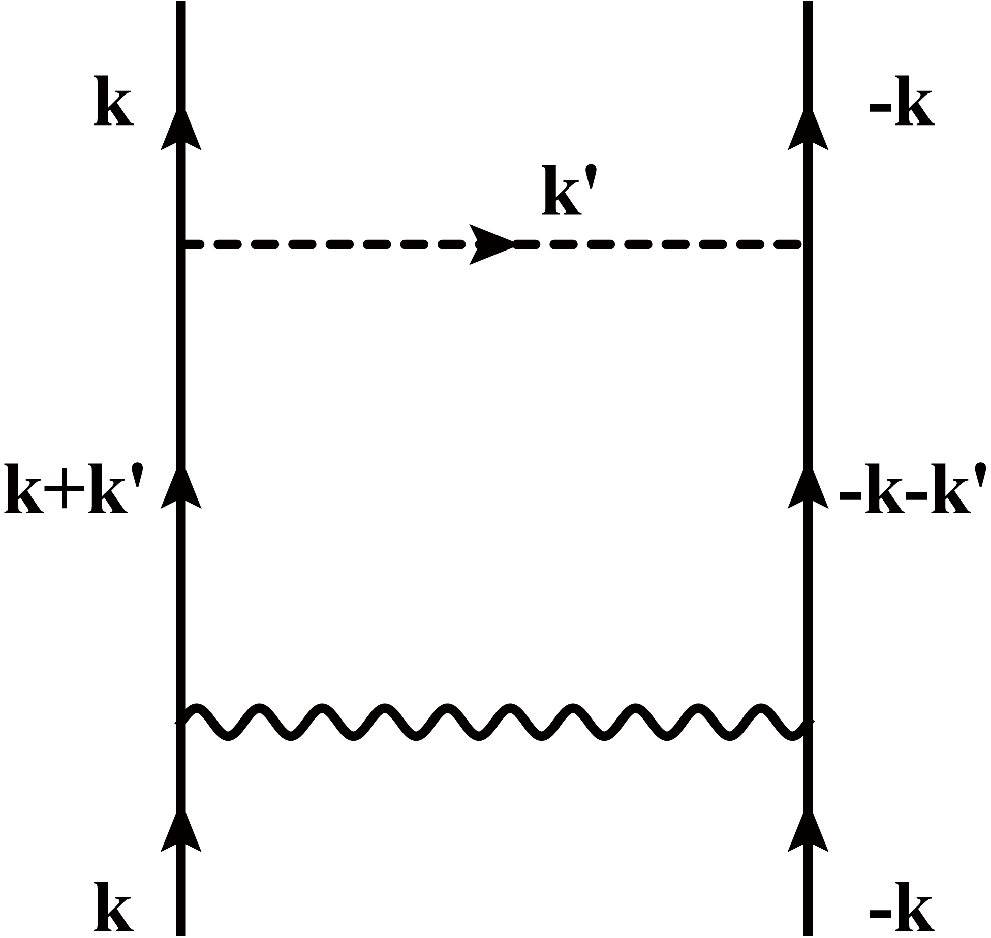
which serve as our starting point. This effective action contributes the one-loop corrections to the fermionic propagator, the coupling $\lambda$, and the disorder strength as shown in Fig. 1, Fig. 2, and Fig. 3, respectively. It is of particular importance to highlight that the attractive Cooper-channel interaction (4) produces three distinct classes of one-loop diagrams including ZS, $\mathrm{ZS}^{\prime}$, and BCS as shown in Fig. 2 (a)-(c) Shankar1994RMP . These collectively renormalize the coupling strength $\lambda$ and fundamentally govern low-energy physics Shankar1994RMP ; Sondhi2013PRB ; Sondhi2014PRB of the FDSM. We are going to examine the potential emergence of Cooper instability in these fractional Dirac materials under the combined influence of all interaction terms in $S_{\mathrm{eff}}$.

Figure 3: (Color online) One-loop corrections to the fermion-disorder interaction due to (a)-(d) the fermion-disorder interaction and (e) the Cooper interaction. The wave and dashed lines denote the Cooper-pairing interaction and the fermion-disorder interaction, respectively.

III RG analysis and coupled flow equations

Within this section, we perform a one-loop renormalization group (RG) Wilson1975RMP ; Polchinski9210046 ; Shankar1994RMP analysis of the effective theory (7) to derive coupled flow equations for all relevant parameters as the energy scale is lowered, which are generally crucial to dictate the low-energy physical behavior. To this end, following the spirit of RG approach Wilson1975RMP ; Polchinski9210046 ; Shankar1994RMP , one integrates out the fast-mode fermionic fields within the momentum shell $b\Lambda<|k|<\Lambda$, where $b\equiv e^{-l}<1$ and $l$ is the running energy scale, and then incorporates their corrections into the slow modes, and finally rescales the slow modes to new “fast modes” Huh2008PRB ; Kim2008PRB ; Maiti2010PRB ; She2010PRB ; She2015PRB ; Vafek2012PRB ; Vafek2014PRB ; Roy2016PRB ; Wang2011PRB ; Wang2013PRB ; Wang2017PRB_QBCP .

In order to connect two steps of RG processes, the non-interacting parts of effective action can be considered as a fixed point that is invariant during the RG transformations. This yields the RG rescaling transformations of energies and momenta as well as fields in the momentum-frequency space Shankar1994RMP ; Huh2008PRB ; Wang2011PRB ,

$$k_{x} = k^{\prime}_{x}e^{-l},$$ (8)

$$k_{y} = k^{\prime}_{y}e^{-l},$$ (9)

$$\omega = \omega^{\prime}e^{-\alpha l},$$ (10)

$$\Psi_{\sigma}(i\omega,\mathbf{k}) = \Psi_{\sigma}^{\prime}(i\omega^{\prime},\mathbf{k}^{\prime})e^{\left(\alpha+1-\eta_{f}\right)l},$$ (11)

where $\eta_{f}$ is the anomalous dimension that captures the contribution from the one-loop corrections.

In particular, it is essential to reemphasize that the one-loop corrections to the interaction parameter $\lambda$ decompose into three distinct diagrammatic channels Shankar1994RMP , i.e. ZS, $\mathrm{ZS}^{\prime}$, and BCS subchannels as depicted in Fig. 2 (a)-(c). While both ZS and $\mathrm{ZS}^{\prime}$ diagrams feature finite transfer momenta $\mathbf{Q}=\mathbf{q}-\mathbf{k}$ and $\mathbf{Q}^{\prime}=-\mathbf{q}-\mathbf{k}$ respectively, under the Cooper interaction, it is restricted with $|\mathbf{Q}|\ll|\mathbf{Q}^{\prime}|$ once two external momenta $\mathbf{q}$ and $\mathbf{k}$ possess the same sign or $|\mathbf{Q}^{\prime}|\ll|\mathbf{Q}|$ if they own opposite signs Shankar1994RMP . In this sense, we adopt the approximation $\mathbf{Q}\approx 0$ while retaining finite $\mathbf{Q}^{\prime}$ or vice versa Shankar1994RMP ; Wang2017PRB_BCS . Hereby, the finite transfer momentum can be parameterized as $\mathbf{Q}=Q(\cos\phi,\sin\phi)$ where $Q$ and $\phi$ denote magnitude and angular orientation, respectively. Paralleling the analogous procedures in Refs. Vafek2014PRB ; Wang2017PRB_QBCP ; DZZW2020PRB ; Huh2008PRB ; Maiti2010PRB ; She2010PRB ; Wang2011PRB ; Wang2013PRB ; Kim2008PRB ; She2015PRB ; Roy2016PRB ; Nandkishore2012NP and carrying out lengthy but straightforward calculations, we derive the anomalous dimension as

$$\eta_{f}=\frac{\mathcal{F}_{5}}{16\pi^{2}v_{\alpha}^{2}}\sum_{j=0}^{3}\Delta_{i},$$ (12)

and all one-loop corrections for the Cooper pairing interaction

$$\delta\lambda=\!\left\{\begin{matrix}\frac{\lambda^{2}\Lambda^{4}l}{8\pi^{2}v_{\alpha}}\!\left[\mathcal{F}_{4}-\frac{(\mathcal{F}_{0}+v_{\alpha}\mathcal{F}_{1})}{2}-\frac{3}{8v_{\alpha}^{4}}\mathcal{F}_{12}\right]\mathbf{Q}\neq 0,\mathbf{Q}^{\prime}=0,\\ \\ \frac{\lambda^{2}\Lambda^{4}l}{8\pi^{2}v_{\alpha}}\!\left[\mathcal{F}_{4}-\frac{(\mathcal{F}_{0}^{\prime}+v_{\alpha}\mathcal{F}_{1}^{\prime})}{2}-\frac{3}{8v_{\alpha}^{4}}\mathcal{F}_{12}\right]\mathbf{Q}=0,\mathbf{Q}^{\prime}\neq 0,\end{matrix}\right.$$ (13)

as well as

$$\delta\Delta_{0} = \frac{l}{4\pi^{2}}\left(\frac{\Delta_{0}^{2}}{v_{\alpha}^{2}}\mathcal{F}_{11}\right),$$ (14)

$$\delta\Delta_{1} = \frac{l}{4\pi^{2}}\left(\frac{\lambda}{16}\Delta_{1}\mathcal{F}_{3}-2\Delta_{1}^{2}\frac{1}{v_{\alpha}^{2}}\mathcal{F}_{2}\right),$$ (15)

$$\delta\Delta_{2} = \frac{l}{4\pi^{2}}\left[\frac{\lambda}{16}\Delta_{2}\mathcal{F}_{4}-\left(\lambda\Delta_{2}-2\Delta_{2}^{2}\right)\frac{1}{v_{\alpha}^{2}}\mathcal{F}_{2}\right],$$ (16)

$$\delta\Delta_{3} = \frac{l}{4\pi^{2}}\left[\frac{\lambda}{16}\Delta_{3}\left(2\mathcal{F}_{3}+\mathcal{F}_{4}\right)+2\Delta_{3}^{2}\frac{1}{v_{\alpha}^{2}}\mathcal{F}_{5}\right],$$ (17)

for the disorder strengths, where all the related coefficients are provided in Appendix A.

To proceed, following the standard procedures of RG approach Shankar1994RMP with the help of the RG rescaling transformations (8)-(11), in tandem with the one-loop corrections (12)-(17), the coupled RG equations of all interactions in the effective action can be derived as,

$$\frac{dv_{\alpha}}{dl} = -\frac{\mathcal{F}_{5}}{8\pi^{2}}\sum_{j=0}^{3}\frac{\Delta_{j}}{v_{\alpha}},$$ (18)

$$\frac{d\lambda}{dl} = \lambda\left[(\alpha-2)-\frac{\mathcal{F}_{0}+v_{\alpha}\mathcal{F}_{1}}{4\pi^{2}v_{\alpha}}\lambda-\frac{\mathcal{F}_{5}}{4\pi^{2}}\sum_{j=0}^{3}\Delta_{j}\right],$$ (19)

and

$$\frac{d\Delta_{0}}{dl} = \left[2(\alpha-1)+\frac{\mathcal{F}_{5}}{4\pi^{2}}\frac{\Delta_{0}-\Delta_{1}-\Delta_{2}-\Delta_{3}}{v_{\alpha}^{2}}\right]\Delta_{0},$$ (20)

$$\frac{d\Delta_{1}}{dl} = \left[2(\alpha-1)+\frac{\mathcal{F}_{3}}{32\pi^{2}}\lambda-\frac{\mathcal{F}_{2}}{\pi^{2}}\frac{\Delta_{1}}{v_{\alpha}^{2}}-\frac{\mathcal{F}_{5}}{4\pi^{2}}\sum_{j=0}^{3}\frac{\Delta_{j}}{v_{\alpha}^{2}}\right]\Delta_{1},$$ (21)

$$\frac{d\Delta_{2}}{dl} = \left[2(\alpha-1)+\frac{\mathcal{F}_{4}}{32\pi^{2}}\lambda-\frac{\mathcal{F}_{2}}{2\pi^{2}}\frac{\lambda-2\Delta_{2}}{v_{\alpha}^{2}}-\frac{\mathcal{F}_{5}}{4\pi^{2}}\sum_{j=0}^{3}\frac{\Delta_{j}}{v_{\alpha}^{2}}\right]\Delta_{2},$$ (22)

$$\frac{d\Delta_{3}}{dl} = \left[2(\alpha-1)+\frac{2\mathcal{F}_{3}+\mathcal{F}_{4}}{32\pi^{2}}\lambda+\frac{\mathcal{F}_{5}}{4\pi^{2}}\frac{3\Delta_{3}-\Delta_{0}-\Delta_{1}-\Delta_{2}}{v_{\alpha}^{2}}\right]\Delta_{3},$$ (23)

for the case $\mathbf{Q}\neq 0,\mathbf{Q}^{\prime}=0$, and

$$\frac{dv_{\alpha}}{dl} = -\frac{\mathcal{F}_{5}}{8\pi^{2}}\sum_{j=0}^{3}\frac{\Delta_{j}}{v_{\alpha}},$$ (24)

$$\frac{d\lambda}{dl} = \lambda\left[(\alpha-2)-\frac{\mathcal{F}_{0}^{\prime}+v_{\alpha}\mathcal{F}_{1}^{\prime}}{4\pi^{2}v_{\alpha}}\lambda-\frac{\mathcal{F}_{5}}{4\pi^{2}}\sum_{j=0}^{3}\Delta_{j}\right],$$ (25)

and

$$\frac{d\Delta_{0}}{dl} = \left[2(\alpha-1)+\frac{\mathcal{F}_{5}}{4\pi^{2}}\frac{\Delta_{0}-\Delta_{1}-\Delta_{2}-\Delta_{3}}{v_{\alpha}^{2}}\right]\Delta_{0},$$ (26)

$$\frac{d\Delta_{1}}{dl} = \left[2(\alpha-1)+\frac{\mathcal{F}_{3}}{32\pi^{2}}\lambda-\frac{\mathcal{F}_{2}}{\pi^{2}}\frac{\Delta_{1}}{v_{\alpha}^{2}}-\frac{\mathcal{F}_{5}}{4\pi^{2}}\sum_{j=0}^{3}\frac{\Delta_{j}}{v_{\alpha}^{2}}\right]\Delta_{1},$$ (27)

$$\frac{d\Delta_{2}}{dl} = \left[2(\alpha-1)+\frac{\mathcal{F}_{4}}{32\pi^{2}}\lambda-\frac{\mathcal{F}_{2}}{2\pi^{2}}\frac{\lambda-2\Delta_{2}}{v_{\alpha}^{2}}-\frac{\mathcal{F}_{5}}{4\pi^{2}}\sum_{j=0}^{3}\frac{\Delta_{j}}{v_{\alpha}^{2}}\right]\Delta_{2},$$ (28)

$$\frac{d\Delta_{3}}{dl} = \left[2(\alpha-1)+\frac{2\mathcal{F}_{3}+\mathcal{F}_{4}}{32\pi^{2}}\lambda+\frac{\mathcal{F}_{5}}{4\pi^{2}}\frac{3\Delta_{3}-\Delta_{0}-\Delta_{1}-\Delta_{2}}{v_{\alpha}^{2}}\right]\Delta_{3},$$ (29)

for the case $\mathbf{Q}=0,\mathbf{Q}^{\prime}\neq 0$. All the related coefficients are presented in Appendix A.

Figure 4: (Color online) Schematic illustration of the flow divergence for the Cooper channel coupling strength $\lambda$ when the initial coupling $|\lambda_{0}|$ exceeds the critical threshold $|\lambda_{c}|$.

Before proceeding, we highlight essential characteristics of above coupled RG evolutions for interaction parameters. These equations render all couplings interdependent and thus their low-energy fates are intimately associated with each other. Consequently, the low-energy behavior may deviate significantly from tree-level counterparts, potentially undergoing either quantitative or qualitative modifications. Of particular importance is the renormalization of coupling $\lambda$, which may flow toward strong-coupling regimes and potentially induce Cooper instability under certain conditions. In the following sections, we are going to investigate whether Cooper instability can be generated and how the system parameters govern its emergence.

IV Potential Cooper instability at clean limit

Using the coupled renormalization group (RG) equations (18)-(23) for $\mathbf{Q}\neq 0,\mathbf{Q}^{\prime}=0$ and (24)-(29) for $\mathbf{Q}=0,\mathbf{Q}^{\prime}\neq 0$, we analyze the low-energy evolution of the Cooper interaction strength $\lambda$. At tree level, these RG equations reduce to

$$\frac{dv}{dl} = 0,\hskip 8.5359pt\frac{d\lambda}{dl}=(\alpha-2)\lambda,$$ (30)

where $\alpha\in(0,1)$ characterizes the fractional dispersion in the FDSM Roy2023PRR . In this circumstance, $\lambda$ decreases monotonically as the energy scale decreases. Accordingly, the Cooper instability is strictly forbidden. We subsequently turn attention to how one-loop corrections modify this behavior. As mentioned in Sec. III, the transfer momenta $\mathbf{Q}$ and $\mathbf{Q^{\prime}}$ cluster into two distinct scenarios, namely Scenario-A and Scenario-B for $\mathbf{Q}\neq 0$, $\mathbf{Q^{\prime}}=0$ and $\mathbf{Q}=0$, $\mathbf{Q^{\prime}}\neq 0$, respectively. Without loss of generality, we primarily examine the physical behavior in Scenario-A and address the discussion of Scenario-B for the end of this section. For clarity, we restrict this section to the clean limit and defer disorder effects to Section V.

IV.1 Warm up: preliminary approximation analysis

In the clean limit, the disorder parameters $\Delta_{i}$ (for $i=1,2,3$) vanish, reducing the RG equation for the Cooper interaction to

$$\frac{d\lambda}{dl} = \lambda\left[(\alpha-2)-\frac{\lambda}{4\pi^{2}v_{\alpha}}\left(\mathcal{F}_{0}+v_{\alpha}\mathcal{F}_{1}\right)\right],$$ (31)

where the fermionic velocity $v_{\alpha}$ is a $l$-independent constant, and the coefficients $\mathcal{F}_{0}$ and $\mathcal{F}_{1}$ are defined in Eq. (35) and Eq. (36), respectively.

Figure 5: (Color online) The critical coupling strength $|\lambda_{c}|$ required for Cooper instability with the fractional exponent $\alpha=0.3$ and three fermionic velocities (a) $v_{\alpha}=10^{-3}$, (b) $10^{-4}$, and (c) $10^{-5}$. The parameter space partitions into two distinct sectors: Zone-I (white) and Zone-II (colored) where the Cooper instability is prohibited and permitted at $|\lambda_{0}|>|\lambda_{c}|$.

As a warm-up, let us assume $\mathcal{F}_{0}$ and $\mathcal{F}_{1}$ to be two constants and provide an attentive and preliminary analysis of the behavior of Cooper interaction. For convenience, we introduce $a\equiv\alpha-2$ and $b\equiv-\frac{(\mathcal{F}_{0}+\mathcal{F}_{1}v_{\alpha})}{4\pi^{2}v_{\alpha}}$ and thus Eq. (31) is cast into a compact form

$$\frac{d\lambda}{dl}=a\lambda+b\lambda^{2}.$$ (32)

It can be found that the evolution of $\lambda$ is governed by the sign of its slope. On one hand, a positive slope with $d\lambda/dl>0$ indicates that $\lambda$ increases toward asymptotic stability at $\lambda=0$, thus suppressing the BCS instability. On the other hand, a negative slope causes $\lambda$ to toward strong-coupling divergence, which is an indicator of BCS instability Shankar1994RMP ; Zhao2006PRL ; Honerkamp2008PRL ; Sondhi2013PRB ; Sondhi2014PRB .

Figure 6: (Color online) The critical interaction strength $|\lambda_{c}|$ required for Cooper instability with fixing the fermionic velocity $v_{\alpha}=10^{-3}$ and tuning the parameter $\alpha$ as (a) $10^{-4}$, (b) $10^{-3}$, (c) $10^{-2}$, (d) $10^{-1}$, (e) 0.25, (f) 0.50, (g) 0.61, and (h) 0.75.

In this sense, taking $d\lambda/dl=0$ yields two critical points $\lambda_{c}=0$ and $\lambda_{c}=-a/b$. Since $\lambda_{c}=0$ is trivial, we put the focus on the latter. As illustrated in Fig. 4, the Cooper interaction $\lambda$ goes towards divergence as long as the following initial condition satisfies

$$\left|\lambda_{0}\right|>|\lambda_{c}|=\frac{4(2-\alpha)\pi^{2}v_{\alpha}}{\mathcal{F}_{0}+\mathcal{F}_{1}v_{\alpha}}.$$ (33)

This inequality represents a preliminary criterion for Cooper instability with all related coefficients being constant. However, both $\mathcal{F}_{0}$ and $\mathcal{F}_{1}$ are not constants but dependent on other parameters. It is necessary to go beyond the coarse analytical analysis and examine this more systematically.

IV.2 Critical Cooper strength of Scenario-A

Subsequently, let us examine the tendency of critical strength $|\lambda_{c}|$ at clean limit, which is composed of $v_{\alpha}$ as well as the parameters $(\alpha,Q,\phi)$.

At the outset, we find from Fig. 5 that the variation of $v_{\alpha}$ can only provide quantitative effects on the value of $\lambda_{c}$ but do not qualitatively modify the overall structure of dependence of other parameters. It is of particular importance to highlight that there yield two distinct regions in the $Q$-$\phi$ space, which are designated as $\text{Zone-}\mathrm{I}$ and $\text{Zone-}\mathrm{II}$, corresponding to the white region and the colored region in Fig. 5, respectively. As to the former, $\mathcal{F}_{0}+\mathcal{F}_{1}v_{\alpha}<0$ implies that the BCS instability is strictly forbidden, but instead $\frac{4(2-\alpha)\pi^{2}v_{\alpha}}{\mathcal{F}_{0}+\mathcal{F}_{1}v_{\alpha}}>0$ for the latter and thus the BCS instability is available at $|\lambda_{0}|>|\lambda_{c}|$. Reading off Fig. 5, it is clear that the shapes of Zone-I and Zone-II is insensitive to the variation of $v_{\alpha}$ which only causes $|\lambda_{c}|$ to change. As a consequence, the $v_{\alpha}$ is subordinate to other parameters in impacting the BCS criterion that is primarily determined by the $\text{Zone-}\mathrm{II}$. To simplify the analysis, we take $v_{\alpha}=10^{-3}$ in the following discussions.

Next, let us consider the influence of the fractional exponent $\alpha$ on the Cooper instability. Fig. 6 illustrates that the areas of Zone-I and Zone-II are highly sensitive to the value of $\alpha$. To be concrete, Fig. 6 presents that there exist two critical values, $\alpha_{c1}\approx 10^{-3}$ and $\alpha_{c2}\approx 0.61$. As $\alpha$ increases from a very small value, Zone-I emerges at $\alpha=\alpha_{c1}$, then expands, contracts, and finally disappears beyond $\alpha=\alpha_{c2}$ as shown in Fig. 6(a)-(d). This implies that within the region $\alpha\in(\alpha_{c1},\alpha_{c2})$, Zone-I and Zone-II can coexist and compete with each other, while Zone-II dominates when $\alpha<\alpha_{c1}$ or $\alpha>\alpha_{c2}$. Besides, Fig. 6(e)-(h) clearly show that the increase of $\alpha$ is helpful to enlarge the blue portion of Zone-II, where the critical strength of Cooper interaction $|\lambda|$ decreases. This indicates that a higher $\alpha$ favors the emergence of BCS instability.

Furthermore, we examine the effects of transfer momentum characterized by momentum magnitude $Q$ and angular orientation $\phi$ on the critical strength of Cooper interaction. As depicted in Fig. 6, the response to $Q$-variation is strongly modulated by $\phi$. For orientations near $\phi\approx 0$ or $2\pi$, the critical strength $|\lambda_{c}|$ decreases monotonically with increasing $Q$. In sharp contrast, $|\lambda_{c}|$ exhibits the inverse behavior near $\phi\approx\pi$. Specifically, at low momentum scales, $|\lambda_{c}|$ shows insensitive variation with $\phi$, reflecting weak directional dependence. Conversely, in the high-momentum regime, it displays angular dependence, first increasing and then decreasing as $\phi$ is tuned from $0$ to $2\pi$. Additionally, for $\alpha\in(\alpha_{c1},\alpha_{c2})$, when $Q$ and $\phi$ take appropriate values, the critical strength $|\lambda_{c}|$ goes toward infinity. This indicates that the Cooper instability is forbidden, corresponding to the emergence of $\text{Zone-}\mathrm{I}$ which is shown as the white region in Fig. 6.

IV.3 Fate of Cooper interaction for Scenario-A

To move forward, let us combine the RG behavior of $\lambda$ (31) and the constraints on critical strength $\lambda_{c}$ from previous subsections to examine the energy-dependent behavior of $\lambda$. Fig. 7 illustrates the energy-dependent behavior of $\lambda$ under different conditions associated with Fig. 6. We find that the RG analysis of $\lambda$ is well consistent with the study of critical Cooper strength in Sec. IV.2.

Figure 7: (Color online) Energy-dependent evolutions of the relative interaction strength $|\lambda|/|\lambda_{0}|$ with variations of the parameter $\alpha$ at specific points in the $(Q,\phi)$ parameter space from Fig. 6: (a) $Q=0.01,\phi=\pi/4$, (b) $Q=0.01,\phi=\pi$, (c) $Q=0.01,\phi=7\pi/4$, and (d) $Q=0.005,\phi=\pi$.

Figure 8: (Color online) Energy-dependent evolution of the relative interaction strength $|\lambda|/|\lambda_{0}|$ at $(Q=0.01,\phi=\pi)$ (from Fig. 6), varying the initial values: Cooper interaction $|\lambda_{0}|$ in (a) $10^{-1}$, (b) $10^{-2}$, (c) $10^{-3}$, as well as the parameter $\alpha$ in (d) $10^{-2}$, (e) $10^{-4}$, and (f) $10^{-5}$.

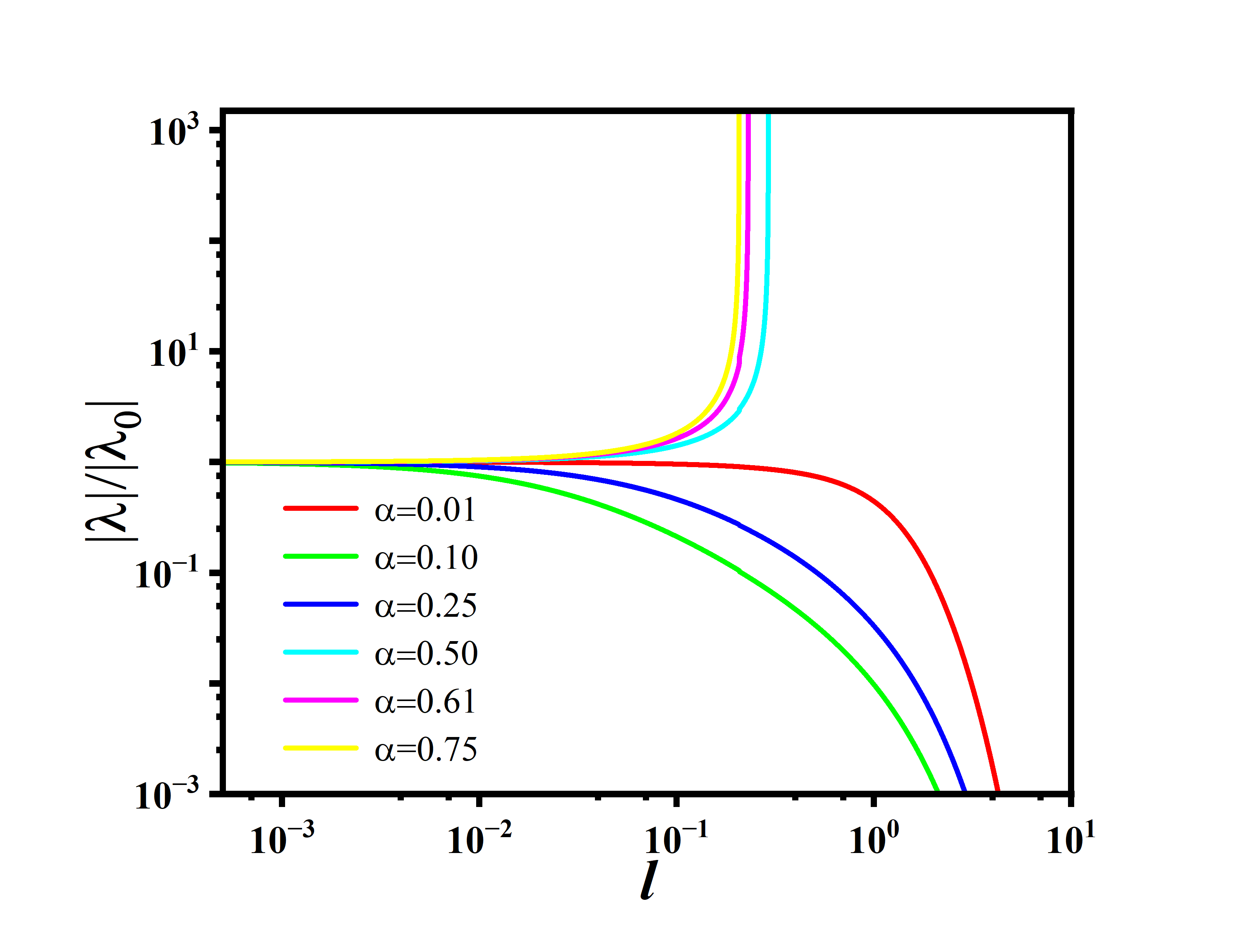
At first, paralleling Fig. 6, let us focus on the influence of fractional dispersion index. By selecting $(Q=0.01,\phi=\pi/4)$, where $|\lambda_{c}|$ is relatively small, and varying the dispersion index $\alpha$, we notice from Fig. 7(a) that the $\lambda$ always goes towards certain instability as long as $|\lambda_{0}|$ exceeds the critical value depicted in Fig. 6(a). Besides, Fig. 7(c) at $(Q=0.01,\phi=7\pi/4)$ exhibits analogous divergent behavior to Fig. 7(a). As a consequence, the evolution of $\lambda$ is insensitive to the value of $\alpha$ in the situation with small $Q$ and $\phi$, and a smaller $\phi$ is more helpful to the emergence of the Cooper instability. In comparison, when $Q$ and $\phi$ are properly chosen, the parameter $\alpha$ can impose a significant influence. As depicted in Fig. 7(b) with $(Q,\phi)=(0.01,\pi)$ and Fig. 7(d) with $(Q,\phi)=(5\times 10^{-3},\pi)$, we consider the intermediate region in Fig. 6 while maintaining the same value of the initial Cooper strength $\lambda_{0}$. From Fig. 7(b) and Fig. 7(d), it is evident that $\lambda$ diverges and Cooper instability emerges for $\alpha\geq 0.50$, whereas for smaller $\alpha\leq 0.25$, $\lambda$ gradually diminishes and Cooper instability does not occur. This accordingly exists a critical threshold of fractional exponent for Cooper instability. All these results are well in agreement with the prior analysis of critical Cooper interaction determined by parameters $(\alpha,Q,\phi)$ in Fig. 6.

Then, we fix the parameters $(Q,\phi)$ and turn to investigate how the initial values of $\lambda_{0}$ and $v_{\alpha}$ affect the Cooper instability, which are demonstrated in Fig. 8. Figs. 8(a)-(c) show that with $v_{\alpha}$ fixed, increasing $|\lambda_{0}|$ is helpful to trigger the Cooper instability. In sharp contrast, with fixing $\lambda_{0}$, Fig. 8(d)-(f) present that a smaller $v_{\alpha}$ enhances the possibility for the divergence of Cooper interaction. Therefore, this confirms that strong initial attractions and suppressed fermion kinetics are in cooperatively favour of Cooper instability Shankar1994RMP ; Sondhi2013PRB ; Sondhi2014PRB .

Table 1: Basic results of Scenario-A in the clean limit (analogous to Scenario-B under $Q\rightarrow Q^{\prime}$). CI denotes Cooper instability, and NO CI indicates that Cooper instability cannot occur.

Range of $\alpha$	Region of ($Q$, $\phi$)	Behavior
$0<\alpha<\alpha_{c1}$	The entire region	CI triggered at $|\lambda_{0}|>|\lambda_{c}|$
$\alpha_{c1}<\alpha<\alpha_{c2}$	$(Q,\phi)\in$ Zone-I	NO CI
	$(Q,\phi)\in$ Zone-II	CI triggered at $|\lambda_{0}|>|\lambda_{c}|$
$\alpha_{c2}\leq\alpha<1$	The entire region	CI triggered at $|\lambda_{0}|>|\lambda_{c}|$

IV.4 Results for Scenario-B and clean-limit conclusions

To proceed, let us provide brief comments on the Scenario-B. In this circumstance, the RG equation of Cooper interaction (31) is recast into

$$\frac{d\lambda}{dl} = \lambda\left[(\alpha-2)-\frac{\lambda}{4\pi^{2}v_{\alpha}}\left(\mathcal{F}_{0}^{\prime}+v_{\alpha}\mathcal{F}_{1}^{\prime}\right)\right],$$ (34)

where $\mathcal{F}_{0}^{\prime}$ and $\mathcal{F}_{1}^{\prime}$ are designated in Eqs. (37)-(38). Compared with their Scenario-A counterparts $\mathcal{F}_{0}$ and $\mathcal{F}_{1}$ in Eq. (31), it is worth emphasizing that they possess the same functional dependencies but only replace $Q$ with $Q^{\prime}$. As a consequence, Scenario-B shares the analogous critical behavior of Cooper interaction with Scenario-A presented in Sec. IV.2.

Figure 9: (Color online) Schematic illustration for the influence of parameters $Q$, $\phi$, $\alpha$, and $v_{\alpha}$ on critical strength of Cooper interaction $|\lambda_{c}|$ in Zone-II.

In this sense, we are now in a suitable position to address the primary results at the clean limit. Both analytical and numerical studies indicate that there exists a critical strength of interaction $\lambda$ for Cooper instability in the 2D FDSMs. For either Scenario-A or Scenario-B, such a critical interaction denoted by $\lambda_{c}$ is closely dependent upon the fractional dispersion exponent $\alpha$ and the transfer momentum magnitude $Q$ as well as its angular orientation $\phi$, while the fermionic velocity $v_{\alpha}$ provides a quantitative effect. Table 1 summarizes our primary results. Specifically, the $(Q,\phi)$ parameter space is divided into two distinct regions as displayed in Fig. 5 and Fig. 6. Zone-I with ($\mathcal{F}_{0}+\mathcal{F}_{1}v_{\alpha}<0$) prohibits the divergence of interaction, whereas Zone-II allows for Cooper instability when $|\lambda_{0}|>|\lambda_{c}|$. In particular, $\alpha$ governs the areas of Zone-I and Zone-II via critical thresholds $\alpha_{c1}\approx 10^{-3}$ and $\alpha_{c2}\approx 0.61$ and its increase is helpful to decrease the $|\lambda_{c}|$. Additionally, with increasing $Q$, the $|\lambda_{c}|$ can either increase or decrease depending on the direction of momentum denoted by $\phi$ as schematically illustrated in Fig. 7.

V Impact of disorder scatterings on Cooper instability–doing

In the presence of disorder scatterings, the Cooper interaction strength and disorder parameters as well as fermion velocity become mutually coupled through the coupled RG flows (18)-(29). Crucially, disorder scatterings are possible to induce significant deviations from clean-limit behavior in kinds of semimetals Ramakrishnan1985RMP ; Lerner0307471 ; Nersesyan1995NPB ; Stauber2005PRB ; Wang2011PRB ; Mirlin2008RMP ; Coleman2015Book ; Roy2018PRX . Accordingly, it is of particular importance to investigate how disorder scattering modifies the Cooper instability criteria. Given the analogous critical behavior exhibited in Scenario-A and Scenario-B, we focus exclusively on Scenario A for this analysis, with its RG equations formally expressed in Eqs. (18)-(23).

Figure 10: (Color online) Energy-dependent evolutions of the relative interaction strength $\left|\frac{\lambda-\lambda_{0}}{\lambda_{0}}\right|$ at Point-A and Point-B for (a)-(b) $\alpha=0.25$ and (c)-(d) $\alpha=0.75$ in the sole presence of disorder $\Delta_{0}$, as well as (e)-(f) $\alpha=0.25$ and (g)-(h) $\alpha=0.75$ in the sole presence of disorder $\Delta_{3}$, respectively.

V.1 Single type of disorder

At first, we consider the presence of sole type of disorder scattering. In the clean limit, the fractional exponent $\alpha$ plays a critical role in inducing the Cooper instability by partitioning the $(Q,\phi)$ parameter space into two distinct regions including Zone-I and Zone-II as depicted in Fig. 6. Based on the critical thresholds in Table 1, we select two representative values $\alpha=0.25$ ($\alpha_{c1}<\alpha<\alpha_{c2}$) and $\alpha=0.75$ ($\alpha_{c2}\leq\alpha<1$) to systematically investigate the disorder scattering effects.

Specifically, by analyzing Fig. 6(e) with $\alpha=0.5$ and Fig. 6(h) with $\alpha=0.75$ and taking into account the symmetry of coordinates, we fix the angular orientation at $\phi=\pi$ and choose two distinct momentum magnitudes $Q=10^{-2}$ and $Q=10^{-4}$, which designate two representative points: Point-A $(Q,\phi)=(10^{-2},\pi)$ and Point-B $(Q,\phi)=(10^{-4},\pi)$. At clean limit, Fig. 6(e) shows that Point-A resides in Zone-I where the condition ($\mathcal{F}_{0}+\mathcal{F}_{1}v_{\alpha}<0$) forbids the divergence of interaction, while Point-B lies in Zone-II where Cooper instability emerges when $|\lambda_{0}|$ exceeds the critical threshold $|\lambda_{c}(Q,\phi)|$. In comparison, Fig. 6(h) displays that both points now occupy Zone-II, enabling the Cooper instability above distinct $|\lambda_{c}|$ values.

Subsequently, we bring out the controlled disorder perturbations at these four selected situations Point-A and Point-B at $\alpha=0.5$, as well as Point-A and Point-B at $\alpha=0.75$ to carefully study how disorder scattering influences the emergence of Cooper instability.

We begin by considering the single presence of random chemical potential denoted by $\Delta_{0}$. For $\alpha=0.25$ ($\alpha_{c1}<\alpha<\alpha_{c2}$), Fig. 10(a) and Fig. 10(b) show that the presence of $\Delta_{0}$ at Point-A is incapable of inducing the Cooper instability initially prohibited in the clean limit. This signals that the properties of Zone-I are insensitive to $\Delta_{0}$. In contrast, $\Delta_{0}$ is manifestly harmful to the Cooper instability at Point-B. As shown in Fig. 10(a), $\Delta_{0}$ suppresses interaction divergence even with large initial $|\lambda_{0}|$ values as long as the initial $\Delta_{0}$ is adequate. However, $\Delta_{0}$ fails to prevent the occurrence of Cooper instability if $\Delta_{0}$ is very small and $|\lambda_{0}|$ is sufficiently large such as $\Delta_{0}=10^{-6}$ and $|\lambda_{0}|=10^{-1}$ depicted in Fig. 10(b). This implies that a non-zero $\Delta_{0}$ increases the critical $|\lambda_{c}|$ required for Cooper instability in Zone-II. As to $\alpha=0.75$ ($\alpha_{c2}\leq\alpha<1$), Fig. 10(c) demonstrates that $\Delta_{0}$ hinders the Cooper instability at $|\lambda_{0}|=10^{-2}$, which would otherwise occur in the clean limit as shown in Fig. 6(h). However, Fig. 10(d) presents that increasing $|\lambda_{0}|$ to $10^{-1}$ allows Cooper instability to emerge at both points. This again confirms that $\Delta_{0}$ hinders Cooper instability by increasing the critical interaction threshold and cannot alter the prohibitive nature of Zone-I.

Table 2: Influence of single presence of disorder on the critical value $|\lambda_{c}|$ for Cooper instability. The symbols $\uparrow$ and $\downarrow$ signify the expansion and contraction of Zone-I and Zone-II which are designated in Sec. IV.2.

Sole disorder	${\color[rgb]{1,0,0}\Delta_{0}}$	${\color[rgb]{0,255,0}\Delta_{1}}$	${\color[rgb]{0,255,0}\Delta_{2}}$	${\color[rgb]{1,0,0}\Delta_{3}}$
Area of Zone-I	${\color[rgb]{1,0,0}\uparrow}$	${\color[rgb]{0,255,0}\downarrow}$	${\color[rgb]{0,255,0}-}$	${\color[rgb]{1,0,0}\uparrow}$
Area of Zone-II	${\color[rgb]{1,0,0}\downarrow}$	${\color[rgb]{0,255,0}\uparrow}$	${\color[rgb]{0,255,0}-}$	${\color[rgb]{1,0,0}\downarrow}$

Figure 11: (Color online) Energy-dependent evolutions of the relative interaction strength $\left|\frac{\lambda-\lambda_{0}}{\lambda_{0}}\right|$ at Point-A and Point-B for (a)-(b) $\alpha=0.25$ and (c)-(d) $\alpha=0.75$ in the sole presence of disorder $\Delta_{1}$, (e)-(f) $\alpha=0.25$ and (g)-(h) $\alpha=0.75$ in the sole presence of disorder $\Delta_{2}$, respectively.

Then, we shift our focus to the sole presence of random gauge potential, which is characterized by two components, $\Delta_{1}$ and $\Delta_{3}$. Fig 10(e) and Fig 10(h) present that the effects of $\Delta_{3}$ component is similar to those of $\Delta_{0}$ on the Cooper interaction. In this sense, we are going to concentrate on the influence of the $\Delta_{1}$ component.

Learning from Fig. 11(a) and Fig. 11(b) for $\alpha=0.25$, the Cooper interaction goes towards divergence with variations of initial conditions of $\Delta_{1}$ at Point-B, which is consistent with the clean-limit results. As aforementioned in Fig. 6(e) the Cooper instability is forbidden in the clean limit for $\alpha=0.25$ at Point-A in Zone-I. In the presence $\Delta_{1}$ presented in Fig. 11(a) and Fig. 11(b), it is indeed absent of Cooper instability when the initial value of $\Delta_{1}$ is small but increasing the initial value of $\Delta_{1}$ to $10^{-2}$, the divergence of Cooper interaction is induced. Further analysis of Fig. 11(c) and (d) shows that the introduction of disorder $\Delta_{1}$ with an initial value of $|\lambda_{0}|=10^{-3}$, which is insufficient to induce the Cooper instability, can clearly drive the divergence of Cooper interaction at either Point-A or Point-B for $\alpha=0.75$. As a corollary, this indicates that the disorder $\Delta_{1}$ effectively reduces the critical threshold $|\lambda_{c}|$ for the Cooper interaction and thus can induce the Cooper instability with a proper initial value where it is prohibited at clean limit.

Moreover, we examine the effects of the sole presence of random mass measured by $\Delta_{2}$.

Fig. 11(e)-11(h) illustrate that, similar to $\Delta_{1}$, disorder $\Delta_{2}$ reduces the critical coupling strength $|\lambda_{c}|$ in Zone-II. Nevertheless, it cannot induce the Cooper instability at Point-A in Zone-I. This sharply contrasts with the unique ability of $\Delta_{1}$ to trigger the divergence of the Cooper interaction at Point-A in Zone-I. In this sense, this establishes that while both $\Delta_{1}$ and $\Delta_{2}$ are helpful to reduce $|\lambda_{c}|$, $\Delta_{1}$ has a stronger influence on inducing the Cooper instability in Zone-I.

To recapitulate, the effects of single disorders fall into two categories. On one hand, $\Delta_{0}$ and $\Delta_{3}$ tend to suppress the divergence of the Cooper interaction but do not alter the regions of Zone-I and Zone-II. On the other hand, $\Delta_{1}$ and $\Delta_{2}$ are both effective in reducing the critical threshold ($|\lambda_{c}|$). Additionally, $\Delta_{1}$ can modify the regions of Zone-II. Table 2 summarizes the key results for the sole presence of disorder scattering.

Figure 12: (Color online) Energy-dependent evolutions of the relative interaction strength $\left|\frac{\lambda-\lambda_{0}}{\lambda_{0}}\right|$ at $\alpha=0.25$ in the presence of two kinds of disorders: (a) Point-A ($\Delta_{0}$, $\Delta_{1}$), (b) Point-B ($\Delta_{0}$, $\Delta_{1}$), (c) Point-A ($\Delta_{0}$, $\Delta_{2}$), (d) Point-B ($\Delta_{0}$, $\Delta_{2}$), (e) Point-A ($\Delta_{1}$, $\Delta_{2}$), (f) Point-B ($\Delta_{1}$, $\Delta_{2}$), (g) Point-A ($\Delta_{1}$, $\Delta_{2}$), and (h) Point-B ($\Delta_{1}$, $\Delta_{2}$).

Table 3: Influence of simultaneous presence of two kinds of disorders on the critical value $|\lambda_{c}|$ for Cooper instability. The symbols $\uparrow$ and $\downarrow$ signify the expansion and contraction of Zone-I and Zone-II which are designated in Sec. IV.2.

Two types of disorder	${\color[rgb]{1,0,0}\Delta_{0},\Delta_{1}}$	${\color[rgb]{1,0,0}\Delta_{0},\Delta_{2}}$	${\color[rgb]{0,255,0}\Delta_{1},\Delta_{2}}$	${\color[rgb]{1,0,0}\Delta_{0},\Delta_{3}}$
Area of Zone-I	${\color[rgb]{1,0,0}\uparrow}$	${\color[rgb]{1,0,0}\uparrow}$	${\color[rgb]{0,255,0}\uparrow}$	${\color[rgb]{1,0,0}\uparrow}$
Area of Zone-II	${\color[rgb]{1,0,0}\downarrow}$	${\color[rgb]{1,0,0}\downarrow}$	${\color[rgb]{0,255,0}\downarrow}$	${\color[rgb]{1,0,0}\downarrow}$

V.2 Two types of disorders

Next, we study the situation in the presence of two types of disorder scatterings. By analyzing the effects of sole presence of disorder as presented in Table 2, it is evident that the impact of $\Delta_{3}$ is analogous to that of $\Delta_{0}$. We therefore turn attention to the combined influence of two of disorder scatterings from $\Delta_{0}$, $\Delta_{1}$, and $\Delta_{2}$ on the fate of Cooper interaction.

Specifically, let us consider the simultaneous presence of $\Delta_{0}$ and $\Delta_{1}$. At Point-A ($Q=10^{-2}$, $\phi=\pi$), as shown in Sec. V.1, $\Delta_{1}$ alone can drive Point-A from Zone-I to Zone-II. However, when both $\Delta_{1}$ and $\Delta_{0}$ are present, Fig. 12(a) demonstrates that any finite $\Delta_{0}$ would completely suppresses this transition regardless of the magnitude of $\Delta_{1}$. Turning to Point-B ($Q=10^{-2}$, $\phi=\pi$), Fig. 12(b) shows that when $\Delta_{0}$ is very small (such as $\Delta_{0}=10^{-6}$), the Cooper interaction can go towards divergence with $\Delta_{1}=10^{-2}$. However, once $\Delta_{0}$ exceeds $10^{-4}$, $\Delta_{1}$ becomes subordinate to $\Delta_{0}$, and its ability to lower $|\lambda_{c}|$ is significantly reduced, keeping $|\lambda_{c}|$ close to its clean-limit value. This clearly indicates that $\Delta_{0}$ generally dominates over $\Delta_{1}$ when they are present simultaneously.

Then, we substitute the disorder $\Delta_{2}$ for $\Delta_{1}$ and analyze the combined effect of $\Delta_{0}$ and $\Delta_{2}$. It can be noticed from Fig. 12(c) and Fig. 12 (d) that this combination exhibits behavior analogous to that of $\Delta_{0}$ and $\Delta_{1}$. In other words, $\Delta_{0}$ remains dominant in suppressing the Cooper interaction, while $\Delta_{2}$ has a significantly weaker effect than $\Delta_{1}$ under identical conditions and can only slightly reduce the critical value $|\lambda_{c}|$ when $\Delta_{0}$ is very small. Furthermore, Fig. 12(g) and Fig. 12(h) demonstrate that the combination of $\Delta_{0}$ and $\Delta_{3}$ still suppresses the Cooper instability and produces behavior similar to that of each disorder acting alone. In consequence, these corroborate that $\Delta_{0}$ compete with other types of disorders and is the leading ingredient in suppressing the Cooper instability regardless of whether it is paired with $\Delta_{1}$, $\Delta_{2}$, or $\Delta_{3}$.

At the end, we briefly comment on the combined presence of $\Delta_{1}$ with $\Delta_{2}$. In contrast to the single $\Delta_{1}$ case shown in Figs. 11(a)-(b), where Point-A transitions from Zone I to Zone II with $\Delta_{1}(0)=10^{-2}$, Fig. 12(e)-Fig. 12(f) demonstrate that, with $\Delta_{2}$ present, the critical threshold for the divergence of the Cooper interaction is further reduced. This allows the Cooper instability to emerge with a smaller initial value of $\Delta_{1}$ ($\Delta_{1}(0)<10^{-2}$). Accordingly, this indicates that $\Delta_{1}$ and $\Delta_{2}$ do not compete but instead cooperate to promote the Cooper instability by lowering the critical value $|\lambda_{c}|$. Table 3 collects the key results for the presence of two distinct kinds of disorder scatterings.

Figure 13: (Color online) Energy-dependent evolutions of the relative interaction strength $\left|\frac{\lambda-\lambda_{0}}{\lambda_{0}}\right|$ at $\alpha=0.25$ in the presence of multiple kinds of disorders: (a) Point-A ($\Delta_{0}$, $\Delta_{1}$, $\Delta_{2}$), (b) Point-B ($\Delta_{0}$, $\Delta_{1}$, $\Delta_{2}$), (c) Point-A ($\Delta_{0}$, $\Delta_{1}$, $\Delta_{3}$), (d) Point-B ($\Delta_{0}$, $\Delta_{1}$, $\Delta_{3}$), (e) Point-A ($\Delta_{0}$, $\Delta_{2}$, $\Delta_{3}$), (f) Point-B ($\Delta_{0}$, $\Delta_{2}$, $\Delta_{3}$), (g) Point-A ($\Delta_{0}$, $\Delta_{1}$, $\Delta_{2}$, $\Delta_{3}$), and (h) Point-B ($\Delta_{0}$, $\Delta_{1}$, $\Delta_{2}$, $\Delta_{3}$).

V.3 Multiple sorts of disorders

At last, we now investigate the circumstance with multiple types of disorders. As detailed in Sec. V.1 and Sec. V.2, all disorders can be clustered into two distinct categories: a suppressing combination of $\Delta_{0}$ and $\Delta_{3}$, and an enhancing combination of $\Delta_{1}$ and $\Delta_{2}$. To examine the effects of multiple disorders, an effective approach is to introduce a promotive disorder to a suppressive pair, or vice versa.

Reading from Fig. 13(a) and Fig. 13(b), it is clear that introducing a suppressive $\Delta_{0}$ to the enhancing combination of $\Delta_{1}$ and $\Delta_{2}$ significantly reduces the critical value of Cooper interaction. This suppression sabotages the possibility to alter the areas of Zone-I and Zone-II. In contrast, Figs. 13(c)-(f) illustrate that the impact of introducing promotive disorders $\Delta_{1}$ or $\Delta_{2}$ into a suppressive combination of $\Delta_{0}$ and $\Delta_{3}$. As to Point-A, neither $\Delta_{1}$ nor $\Delta_{2}$ is able to induce a transition from Zone-I to Zone-II, thus preventing the emergence of Cooper interaction divergence. With respect to Point-B, Fig. 13(e) shows that the critical Cooper interaction for divergence is insusceptible to the introduction of $\Delta_{2}$. However, the addition of $\Delta_{1}$ is in favor of reducing the critical value $|\lambda_{c}|$ even in the suppressive combination of $\Delta_{0}$ and $\Delta_{3}$ as shown in Fig. 13(d). This is well in agreement with the sole presence of $\Delta_{1}$ which is helpful to promote the Cooper instability.

For completeness, we verify the fates of Cooper interaction in the presence of all kinds of disorders as depicted in Fig. 13(g) and Fig. 13(h). It can be found that the tendencies of Cooper interactions are analogous to the circumstance with adding $\Delta_{1}$ or $\Delta_{2}$ to the $\Delta_{0}$-$\Delta_{3}$ suppressive combination. To wrap up, we summarize the basic results in Table 4 for the presence of multiple kinds of disorder scatterings.

Table 4: Influence of presence of multiple sorts of disorders on the critical value $|\lambda_{c}|$ for Cooper instability. The symbols $\uparrow$ and $\downarrow$ signify the expansion and contraction of Zone-I and Zone-II which are designated in Sec. IV.2.

$\Delta$ combinations	Type of ($Q$, $\phi$) region	Area change
${\color[rgb]{0,255,0}\Delta_{0},\Delta_{1},\Delta_{2}}$	Zone-I	${\color[rgb]{0,255,0}\uparrow}$
	Zone-II	${\color[rgb]{0,255,0}\downarrow}$
${\color[rgb]{1,0,0}\Delta_{0},\Delta_{1},\Delta_{3}}$	Zone-I	${\color[rgb]{1,0,0}\uparrow}$
	Zone-II	${\color[rgb]{1,0,0}\downarrow}$
${\color[rgb]{1,0,0}\Delta_{0},\Delta_{2},\Delta_{3}}$	Zone-I	${\color[rgb]{1,0,0}\uparrow}$
	Zone-II	${\color[rgb]{1,0,0}\downarrow}$
${\color[rgb]{1,0,0}\Delta_{0},\Delta_{1},\Delta_{2},\Delta_{3}}$	Zone-I	${\color[rgb]{1,0,0}-}$
	Zone-II	${\color[rgb]{1,0,0}-}$

VI Summary

In summary, this work investigates the fate of Cooper instability in the low-energy regime of 2D FDSMs under the influence of attractive fermion-fermion interaction and disorder scatterings. To treat these competing physical ingredients on an equal footing, we employ a Wilsonian momentum-shell RG analysis Wilson1975RMP ; Polchinski9210046 ; Shankar1994RMP , which yields the energy-dependent flow equations for all coupling strengths. Employing these RG equations (18)-(29), we systematically examine the low-energy fate of Cooper pairing in the clean limit and the presence of disorder scatterings, with particular emphasis on its dependence on physical parameters and initial conditions.

Our analysis considers two complementary scenarios, namely Scenario-A ($Q\neq 0,Q^{\prime}=0$) and Scenario-B ($Q=0,Q^{\prime}\neq 0$) that correspond to distinct configurations of the transfer momenta in the ZS and $\mathrm{ZS}^{\prime}$ channels Shankar1994RMP . As Scenario-B shares the basic similar results with Scenario-A due to an underlying exchange symmetry, we focus primarily on Scenario-A. We begin by examining Cooper instability in the clean limit using a combination of analytical and numerical methods. At tree level, the pairing strength $\lambda$ flows to zero with decreasing energy scale, indicating the absence of instability. However, upon including one-loop corrections, we identify a critical threshold of Cooper-pairing interaction denoted by $\lambda_{c}$. This implies that Cooper instability emerges only when the initial interaction strength $|\lambda_{0}|$ exceeds $|\lambda_{c}|$. Numerical results reveal that $\lambda_{c}$ depends sensitively on the fractional dispersion exponent $\alpha$ and the transfer momentum magnitude $Q$ as well as its angular orientation $\phi$, which are summarized in Table 1. By contrast, the fermionic velocity $v_{\alpha}$ only modifies $\lambda_{c}$ quantitatively, without altering qualitative behavior as shown in Fig. 6. Specifically, the $(Q,\phi)$ parameter space divides into two distinct regions illustrated in Fig. 5: Zone-I, where $|\lambda_{c}|$ diverges and Cooper instability is suppressed, and Zone-II, where $|\lambda_{c}|$ remains finite and instability is allowed. Such two zones coexist and compete with each other when $\alpha$ lies between two critical values $\alpha_{c1}$ and $\alpha_{c2}$, but instead Zone-II completely dominates over Zone-I at $\alpha<\alpha_{c1}$ or $\alpha>\alpha_{c2}$. Additionally, we notice from Fig. 6 and Fig. 8 that higher values of $\alpha$ and lower values of $v_{\alpha}$ reduce the critical interaction $|\lambda_{c}|$, thereby enhancing the opportunity for Cooper instability.

Subsequently, moving beyond the idealized clean limit, we systematically investigate how disorder impacts Cooper instability. Three distinct types of disorders dubbed by $\Delta_{0}$, $\Delta_{1,3}$, and $\Delta_{2}$ Nersesyan1995NPB ; Stauber2005PRB ; Wang2011PRB ; Mirlin2008RMP ; Coleman2015Book ; Roy2018PRX are taken into account. In the presence of single type of disorder, we find that either $\Delta_{0}$ or $\Delta_{3}$ not only increases the critical value of $|\lambda_{c}|$ but also alters the regions of Zone-I and Zone-II, indicating that they suppress the Cooper instability. In contrast, either $\Delta_{1}$ or $\Delta_{2}$ reduces the critical value $|\lambda_{c}|$ and hence promotes the Cooper instability as provided in Table 2. When two or more types of disorders coexist, their competing effects lead to a more intricate scenario. Our analysis shows that the simultaneous presence of both promotive disorders ($\Delta_{1}$ and $\Delta_{2}$) together with a single suppressive disorder ($\Delta_{0}$ or $\Delta_{3}$) is in favor of Cooper instability. Notably, $\Delta_{1}$ exhibits a stronger promotive effect than $\Delta_{2}$. However, in configurations involving all disorder types, the combined suppressive influence of $\Delta_{0}$ and $\Delta_{3}$ dominates over the promotive effects of $\Delta_{1}$ and $\Delta_{2}$. The basic results are summarized in Table 3 and Table 4.

These results elucidate distinctive properties of 2D FDSMs, governed by the competition between Cooper pairing and multiple disorder types, and reveal their intricate relationship with superconductivity through the emergence of Cooper instability. We anticipate that our results would be helpful for further studies of low-energy quantum criticality not only in 2D FDSMs, but also in a broader class of Dirac-type materials with anisotropic or fractional band dispersions.

Appendix A Related coefficients

All the coefficients introduced in Sec. III are designated as follows,

$$\mathcal{F}_{0} \equiv \!\!\int_{0}^{2\pi}\!\!\mathrm{d}\theta\left[\frac{3U}{8P^{\frac{3}{2}}}+\frac{3\alpha(2UL+JP)}{8P}-\frac{9\alpha(1+2P^{\frac{1}{2}})LU}{16P^{\frac{5}{2}}}+\frac{3\alpha UL}{8P^{\frac{5}{2}}}-\frac{\left(2P-U\right)}{8P^{\frac{3}{2}}}\right.$$ (35)

$$\left.-\frac{\alpha\left(2L-J\right)}{8P^{\frac{3}{2}}}+\frac{3\alpha L\left(2P-U\right)}{16P^{\frac{5}{2}}}-\frac{5}{8P^{\frac{1}{2}}}+\frac{5\alpha L}{16P^{\frac{3}{2}}}\right]+2\mathcal{F}_{3}-2\mathcal{F}_{4},$$

$$\mathcal{F}_{1} \equiv \!\!\int_{0}^{2\pi}\!\!\mathrm{d}\theta\left[\frac{2U+P}{8P^{\frac{1}{2}}}+\frac{\alpha(UL+PJ+PL)}{4P^{\frac{3}{2}}}-\frac{\alpha L(2U+P)}{16P^{\frac{3}{2}}}\right]\!\!,$$ (36)

$$\mathcal{F}_{0}^{\prime} \equiv \!\!\int_{0}^{2\pi}\!\!\mathrm{d}\theta\left[\frac{3U}{8P^{\frac{3}{2}}}+\frac{3\alpha(2UL^{\prime}+J^{\prime}P)}{8P}-\frac{9\alpha(1+2P^{\frac{1}{2}})L^{\prime}U}{16P^{\frac{5}{2}}}+\frac{3\alpha UL^{\prime}}{8P^{\frac{5}{2}}}-\frac{\left(2P-U\right)}{8P^{\frac{3}{2}}}\right.$$ (37)

$$\left.-\frac{\alpha\left(2L^{\prime}-J^{\prime}\right)}{8P^{\frac{3}{2}}}+\frac{3\alpha L^{\prime}\left(2P-U\right)}{16P^{\frac{5}{2}}}-\frac{5}{8P^{\frac{1}{2}}}+\frac{5\alpha L^{\prime}}{16P^{\frac{3}{2}}}\right]+2\mathcal{F}_{3}-2\mathcal{F}_{4},$$

$$\mathcal{F}_{1}^{\prime} \equiv \!\!\int_{0}^{2\pi}\!\!\mathrm{d}\theta\left[\frac{2U+P}{8P^{\frac{1}{2}}}+\frac{\alpha(UL^{\prime}+PJ^{\prime}+PL^{\prime})}{4P^{\frac{3}{2}}}-\frac{\alpha L^{\prime}(2U+P)}{16P^{\frac{3}{2}}}\right]\!\!,$$ (38)

$$\mathcal{F}_{2} \equiv \!\!\int_{0}^{2\pi}\!\!\!\mathrm{d}\theta\frac{\left|\cos\theta\right|^{2\alpha}-\left|\sin\theta\right|^{2\alpha}}{\left(\left|\cos\theta\right|^{2\alpha}+\left|\sin\theta\right|^{2\alpha}\right)^{2}},\mathcal{F}_{3}\equiv\!\!\int_{0}^{2\pi}\!\!\!\mathrm{d}\theta\frac{\left|\sin\theta\right|^{2\alpha}}{\left(\left|\cos\theta\right|^{2\alpha}+\left|\sin\theta\right|^{2\alpha}\right)^{\frac{3}{2}}},\mathcal{F}_{4}\equiv\!\!\int_{0}^{2\pi}\!\!\!\!\mathrm{d}\theta\frac{\left|\cos\theta\right|^{2\alpha}}{\left(\left|\cos\theta\right|^{2\alpha}+\left|\sin\theta\right|^{2\alpha}\right)^{\frac{3}{2}}},$$ (39)

$$\mathcal{F}_{5} \equiv \!\!\int_{0}^{2\pi}\!\!\!\mathrm{d}\theta\frac{1}{\left(\left|\cos\theta\right|^{2\alpha}+\left|\sin\theta\right|^{2\alpha}\right)},\mathcal{F}_{6}\equiv\!\!\int_{0}^{2\pi}\!\!\!\mathrm{d}\theta\frac{\left|\sin\theta\right|^{2\alpha}}{\left(\left|\cos\theta\right|^{2\alpha}+\left|\sin\theta\right|^{2\alpha}\right)^{\frac{5}{2}}},\mathcal{F}_{8}\equiv\!\!\int_{0}^{2\pi}\!\!\!\!\mathrm{d}\theta\frac{1}{\left(\left|\cos\theta\right|^{2\alpha}+\left|\sin\theta\right|^{2\alpha}\right)^{2}},$$ (40)

$$\mathcal{F}_{7} \equiv \!\!\int_{0}^{2\pi}\!\!\!\!\mathrm{d}\theta\!\!\left[-\frac{3}{8v_{\alpha}^{3}P^{\frac{3}{2}}}-\frac{3\alpha L}{2v_{\alpha}^{5}P^{\frac{5}{2}}}-\frac{9\alpha(1+2P^{\frac{1}{2}})L+6L}{16v_{\alpha}^{3}P^{\frac{5}{2}}}+\frac{U-4P+\alpha(J-4L)}{4v_{\alpha}^{2}P^{\frac{3}{2}}}-\frac{\alpha L(3+2P)(U-4P)}{8v_{\alpha}^{2}P^{3}}\right]\!\!,$$ (41)

$$\mathcal{F}_{7}^{\prime} \equiv \!\!\int_{0}^{2\pi}\!\!\!\mathrm{d}\theta\!\left[\!\frac{U-4P+\alpha(J^{\prime}-4L^{\prime})}{4v_{\alpha}^{2}P^{\frac{3}{2}}}-\frac{3}{8v_{\alpha}^{3}P^{\frac{3}{2}}}-\frac{3\alpha L^{\prime}}{2v_{\alpha}^{5}P^{\frac{5}{2}}}-\frac{9\alpha(1+2P^{\frac{1}{2}})L^{\prime}+6L^{\prime}}{16v_{\alpha}^{3}P^{\frac{5}{2}}}-\frac{\alpha L^{\prime}(3+2P)(U-4P)}{8v_{\alpha}^{2}P^{3}}\!\right]\!\!,$$ (42)

$$\mathcal{F}_{9} \equiv \!\!\int_{0}^{2\pi}\!\!\!\!\mathrm{d}\theta\frac{\left|\cos\theta\right|^{2\alpha}}{\left(\left|\cos\theta\right|^{2\alpha}+\left|\sin\theta\right|^{2\alpha}\right)^{\frac{5}{2}}},\hskip 28.45274pt\mathcal{F}_{10}\equiv\!\!\int_{0}^{2\pi}\!\!\!\mathrm{d}\theta\frac{3\left|\sin\theta\right|^{2\alpha}-\left|\cos\theta\right|^{2\alpha}}{\left(\left|\cos\theta\right|^{2\alpha}+\left|\sin\theta\right|^{2\alpha}\right)^{3}},$$ (43)

$$\mathcal{F}_{11} \equiv \!\!\int_{0}^{2\pi}\!\!\!\!\mathrm{d}\theta\frac{1}{\left(\left|\cos\theta\right|^{2\alpha}+\left|\sin\theta\right|^{2\alpha}\right)^{3}},\hskip 28.45274pt\mathcal{F}_{12}\equiv\!\!\int_{0}^{2\pi}\!\!\!\!\mathrm{d}\theta\frac{1}{\left(\left|\cos\theta\right|^{2\alpha}+\left|\sin\theta\right|^{2\alpha}\right)^{\frac{5}{2}}},$$ (44)

$$\mathcal{F}_{13} \equiv \!\!\int_{0}^{2\pi}\!\!\!\!\mathrm{d}\theta\frac{1}{\left(\left|\cos\theta\right|^{2\alpha}+\left|\sin\theta\right|^{2\alpha}\right)^{\frac{7}{2}}},\hskip 28.45274pt\mathcal{F}_{14}\equiv\!\!\int_{0}^{2\pi}\!\!\!\!\mathrm{d}\theta\frac{\left|\cos\theta\right|^{2\alpha}}{\left(\left|\cos\theta\right|^{2\alpha}+\left|\sin\theta\right|^{2\alpha}\right)^{\frac{7}{2}}},$$ (45)

$$\mathcal{F}_{15} \equiv \!\!\int_{0}^{2\pi}\!\!\!\mathrm{d}\theta\frac{1}{\left(\left|\cos\theta\right|^{2\alpha}+\left|\sin\theta\right|^{2\alpha}\right)^{\frac{9}{2}}},\hskip 28.45274pt\mathcal{F}_{16}\equiv\!\!\int_{0}^{2\pi}\!\!\!\!\mathrm{d}\theta\frac{\left|\cos\theta\right|^{2\alpha}}{\left(\left|\cos\theta\right|^{2\alpha}+\left|\sin\theta\right|^{2\alpha}\right)^{\frac{9}{2}}},$$ (46)

with

$$P\! \equiv \!\left|\cos\theta\right|^{2\alpha}+\left|\sin\theta\right|^{2\alpha},$$ (47)

$$U\! \equiv \!-\left|\cos\theta\right|^{2\alpha}+\left|\sin\theta\right|^{2\alpha},$$ (48)

$$J\! \equiv \!\left|\sin\theta\right|^{2\alpha-1}\!Q\!\sin\phi-\left|\cos\theta\right|^{2\alpha-1}\!Q\!\cos\phi,$$ (49)

$$L\! \equiv \!\left|\sin\theta\right|^{2\alpha-2}\!Q\!\sin\phi+\left|\cos\theta\right|^{2\alpha-2}\!Q\!\cos\phi,$$ (50)

$$J^{\prime}\! \equiv \!\left|\sin\theta\right|^{2\alpha-1}\!Q^{\prime}\!\sin\phi^{\prime}-\left|\cos\theta\right|^{2\alpha-1}\!Q^{\prime}\!\cos\phi^{\prime},$$ (51)

$$L^{\prime}\! \equiv \!\left|\sin\theta\right|^{2\alpha-2}\!Q^{\prime}\!\sin\phi^{\prime}+\left|\cos\theta\right|^{2\alpha-2}\!Q^{\prime}\!\cos\phi^{\prime}.$$ (52)

Hereby, the finite transfer momentum is parameterized as $\mathbf{Q}=Q(\cos\phi,\sin\phi)$ and $\mathbf{Q}^{\prime}=Q^{\prime}(\cos\phi^{\prime},\sin\phi^{\prime})$, where $Q/Q^{\prime}$ and $\phi/\phi^{\prime}$ denote the magnitude and angular orientation of transfer momentum, respectively.

References

- (1) A. H. Castro Neto, F. Guinea, N. M. R. Peres, K. S. Novoselov, and A. K. Geim, The electronic properties of graphene, Rev. Mod. Phys. 81, 109 (2009).
- (2) M. Z. Hasan and C. L. Kane, Colloquium: Topological insulators, Rev. Mod. Phys. 82, 3045 (2010).
- (3) X. L. Qi and S. C. Zhang, Topological insulators and superconductors, Rev. Mod. Phys. 83, 1057 (2011).
- (4) K. S. Novoselov, A. K. Geim, S. V. Morozov, D. Jiang, M. I. Katsnelson, I. V. Grigorieva, S. V. Dubonos, and A. A. Firsov, Two-dimensional gas of massless Dirac fermions in graphene, Nature 438, 197 (2005).
- (5) L. Fu, C. L. Kane, and E. J. Mele, Topological Insulators in Three Dimensions, Phys. Rev. Lett. 98, 106803 (2007).
- (6) R. Roy, Topological phases and the quantum spin Hall effect in three dimensions, Phys. Rev. B 79, 195322 (2009).
- (7) J. E. Moore, The birth of topological insulators, Nature 464, 194 (2010).
- (8) S. Q. Sheng, Dirac Equation in Condensed Matter (Berlin: Springer, 2012).
- (9) B. A. Bernevig and T. L. Hughes, Topological Insulators and Topological Superconductors (Princeton, NJ: Princeton University Press, 2013).
- (10) A. A. Burkov and L. Balents, Weyl Semimetal in a Topological Insulator Multilayer, Phys. Rev. Lett. 107, 127205 (2011).
- (11) K. Y. Yang, Y. M. Lu, and Y. Ran, Quantum Hall effects in a Weyl semimetal: Possible application in pyrochlore iridates, Phys. Rev. B 84, 075129 (2011).
- (12) X. G. Wan, A. M. Turner, A. Vishwanath, and S. Y. Savrasov, Topological semimetal and Fermi-arc surface states in the electronic structure of pyrochlore iridates, Phys. Rev. B 83, 205101 (2011).
- (13) X. C. Huang, L. X. Zhao, Y. J. Long, P. P. Wang, D. Chen, Z. H. Yang, H. Liang, M. Q. Xue, H. M. Weng, Z. Fang, X. Dai, and G. F. Chen, Observation of the Chiral-Anomaly-Induced Negative Magnetoresistance in 3D Weyl Semimetal TaAs, Phys. Rev. X 5, 031023 (2015).
- (14) S. Y. Xu, I. Belopolski, N. Alidoust, M. Neupane, G. Bian, C. L. Zhang, R. Sankar, G. Q. Chang, Z. J. Yuan, C. C. Lee, S. M. Huang, H. Zheng, J. Ma, D. S. Sanchez, B. K. Wang, A. Bansil, F. C. Chou, P. P. Shibayev, H. Lin, S. Jia, and M. Z. Hasan, Discovery of a Weyl fermion semimetal and topological Fermi arcs, Science 349, 613 (2015).
- (15) S. Y. Xu, N. Alidoust, I. Belopolski, Z. J. Yuan, G. Bian, T. R. Chang, H. Zheng, V. N. Strocov, D. S. Sanchez, G. Q. Chang, C. L. Zhang, D. X. Mou, Y. Wu, L. Huang, C. C. Lee, S. M. Huang, B. K. Wang, A. Bansil, H. T. Jeng, T. Neupert, A. Kaminski, H. Lin, S. Jia, and M. Z. Hasan, Discovery of a Weyl fermion state with Fermi arcs in niobium arsenide, Nat. Phys. 11, 748 (2015).
- (16) B. Q. Lv, N. Xu, H. M. Weng, J. Z. Ma, P. Richard, X. C. Huang, L. X. Zhao, G. F. Chen, C. E. Matt, F. Bisti, V. N. Strocov, J. Mesot, Z. Fang, X. Dai, T. Qian, M. Shi, and H. Ding, Observation of Weyl nodes in TaAs, Nat. Phys. 11, 724 (2015).
- (17) H. Weng, C. Fang, Z. Fang, B. A. Bernevig, and X. Dai, Weyl Semimetal Phase in Noncentrosymmetric Transition-Metal Monophosphides, Phys. Rev. X 5, 011029 (2015).
- (18) Z. J. Wang, Y. Sun, X. Q. Chen, C. Franchini, G. Xu, H. M. Weng, X. Dai, and Z. Fang, Dirac semimetal and topological phase transitions in A3Bi (A=Na, K, Rb), Phys. Rev. B 85, 195320 (2012).
- (19) S. M. Young, S. Zaheer, J. C. Y. Teo, C. L. Kane, E. J. Mele, and A. M. Rappe, Dirac Semimetal in Three Dimensions, Phys. Rev. Lett. 108, 140405 (2012).
- (20) J. A. Steinberg, S. M. Young, S. Zaheer, C. L. Kane, E. J. Mele, and A. M. Rappe, Bulk Dirac Points in Distorted Spinels, Phys. Rev. Lett. 112, 036403 (2014).
- (21) Z. K. Liu, J. Jiang, B. Zhou, Z. J. Wang, Y. Zhang, H. M. Weng, D. Prabhakaran, S. K. Mo, H. Peng, P. Dudin, T. Kim, M. Hoesch, Z. Fang, X. Dai, Z. X. Shen, D. L. Feng, Z. Hussain, and Y. L. Chen, A stable three-dimensional topological Dirac semimetal Cd3As2, Nat. Mater. 13, 677 (2014).
- (22) J. Xiong, S. K. Kushwaha, T. Liang, J. W. Krizan, M. Hirschberger, W. Wang, R. J. Cava, and N. P. Ong, Evidence for the chiral anomaly in the Dirac semimetal Na3Bi, Science 350, 413 (2015).
- (23) Z. K. Liu, B. Zhou, Y. Zhang, Z. J. Wang, H. M. Weng, D. Prabhakaran, S. K. Mo, Z. X. Shen, Z. Fang, X. Dai, Z. Hussain, and Y. L. Chen, Discovery of a Three-Dimensional Topological Dirac Semimetal Na3Bi, Science 343, 864 (2014).
- (24) R. de Gail, J.-N. Fuchs, M.O. Goerbig, F. Piechon, G. Montambaux, Manipulation of Dirac points in graphene-like crystals, Physica B 407, 1948 (2012). M. Goerbig and G. Montambaux, Matière de Dirac, Séminaire Poincaré XVIII, 23-49 (2014).
- (25) R. Nandkishore, J. Maciejko, D. A. Huse, and S. L. Sondhi, Superconductivity of disordered Dirac fermions, Phys. Rev. B 87, 174511 (2013).
- (26) I. D. Potirniche, J. Maciejko, R. Nandkishore, and S. L. Sondhi, Superconductivity of disordered Dirac fermions in graphene, Phys. Rev. B 90, 094516 (2014).
- (27) J. Wang, P. -L. Zhao, J. -R. Wang, and G.-Z. Liu, Superconductivity in two-dimensional disordered Dirac semimetals, Phys. Rev. B 95, 054507 (2017).
- (28) Y. M. Dong, D. X. Zheng, and J. Wang, Cooper instability generated by attractive fermion Cfermion interaction in the two-dimensional semi-Dirac semimetals, J. Phys.: Condens. Matter. 31, 275601 (2019).
- (29) B. Roy and S. D. Sarma, Quantum phases of interacting electrons in three-dimensional dirty Dirac semimetals, Phys. Rev. B 94, 115137 (2016).
- (30) R. M. Nandkishore and S. A. Parameswaran, Disorder-driven destruction of a non-Fermi liquid semimetal studied by renormalization group analysis, Phys. Rev. B 95, 205106 ( 2017).
- (31) M. M. Korshunov, D. V. Efremov, A. A. Golubov and O. V. Dolgov, Unexpected impact of magnetic disorder on multiband superconductivity, Phys. Rev. B 90, 134517 (2014).
- (32) H. H. Hung, A. Barr, E. Prodan and G. A. Fiete, Disorder effects in correlated topological insulators, Phys. Rev. B 94, 235132 (2016).
- (33) H. K. Tang, J. N. Leaw, J. N. B. Rodrigues, I. F. Herbut, P. Sengupta, F. F. Assaad, and S. Adam, The role of electron-electron interactions in two-dimensional Dirac fermions, Science 361, 570 (2018).
- (34) J. Wang, C. Ortix, J. van den Brink, and D. V. Efremov, Fate of interaction-driven topological insulators under disorder, Phys. Rev. B 96, 201104(R) (2017).
- (35) V. Cvetkovic, R. E. Throckmorton, and O. Vafek, Electronic multicriticality in bilayer graphene, Phys. Rev. B 86, 075467 (2012).
- (36) J. M. Murray and O. Vafek, Renormalization group study of interaction-driven quantum anomalous Hall and quantum spin Hall phases in quadratic band crossing systems, Phys. Rev. B 89, 201110(R) (2014).
- (37) K. Sun and E. Fradkin, Time-reversal symmetry breaking and spontaneous anomalous Hall effect in Fermi fluids, Phys. Rev. B 78, 245122 (2008).
- (38) K. Sun, H. Yao, E. Fradkin, and S. A. Kivelson, Topological Insulators and Nematic Phases from Spontaneous Symmetry Breaking in 2D Fermi Systems with a Quadratic Band Crossing, Phys. Rev. Lett. 103, 046811 (2009).
- (39) S. Ray , M. Vojta, and L. Janssen, Soluble fermionic quantum critical point in two dimensions, Phys. Rev. B 102, 081112(R) (2020).
- (40) O. Vafek and K. Yang, Many-body instability of Coulomb interacting bilayer graphene: Renormalization group approach, Phys. Rev. B 81, 041401(R) (2010).
- (41) O. Vafek, Interacting fermions on the honeycomb bilayer: From weak to strong coupling, Phys. Rev. B 82, 205106 (2010).
- (42) W. Zhu, S. S. Gong, T. S. Zeng, L. Fu, and D. N. Sheng, Interaction-Driven Spontaneous Quantum Hall Effect on a Kagome Lattice, Phys. Rev. Lett. 117, 096402 (2016).
- (43) Y. M. Dong, Y. H. Zhai, D. X. Zheng, and J. Wang, Stability of two-dimensional asymmetric materials with a quadratic band crossing point under four-fermion interaction and impurity scattering, Phys. Rev. B 102, 134204 (2020).
- (44) I. F. Herbut, Isospin of topological defects in Dirac systems, Phys. Rev. B 85, 085304 (2012).
- (45) B. Roy, Color degeneracy of topological defects in quadratic band touching systems, arxiv: 2004.13043 (2020).
- (46) I. Mandal and S. Gemsheim, Emergence of topological Mott insulators in proximity of quadratic band touching points, Condens. Matter Phys. 22, 13701 (2019).
- (47) J. Shah and S. Mukerjee, Renormalization group study of systems with quadratic band touching, arxiv: 2011.00249 (2020).
- (48) I. Mandal and R. M. Nandkishore, Interplay of Coulomb interactions and disorder in three-dimensional quadratic band crossings without time-reversal symmetry and with unequal masses for conduction and valence bands, Phys. Rev. B 97, 125121 (2018).
- (49) Y. P. Lin and R. M. Nandkishore, Exotic superconductivity with enhanced energy scales in materials with three band crossings, Phys. Rev. B 97, 134521 (2018).
- (50) J. M. Luttinger, Quantum Theory of Cyclotron Resonance in Semiconductors: General Theory, Phys. Rev. 102, 1030 (1956).
- (51) S. Murakami, N. Nagaosa, and S. C. Zhang, SU(2) non-Abelian holonomy and dissipationless spin current in semiconductors, Phys. Rev. B 69, 235206 (2004).
- (52) L. Janssen and I. F. Herbut, Nematic quantum criticality in three-dimensional Fermi system with quadratic band touching, Phys. Rev. B 92, 045117 (2015).
- (53) I. Boettcher and I. F. Herbut, Superconducting quantum criticality in three-dimensional Luttinger semimetals, Phys. Rev. B 93, 205138 (2016).
- (54) L. Janssen and I. F. Herbut, Phase diagram of electronic systems with quadratic Fermi nodes in 2¡¡4: 2+ expansion, 4? expansion, and functional renormalization group, Phys. Rev. B 95, 075101 (2017).
- (55) I. Boettcher and I. F. Herbut, Anisotropy induces non-Fermi-liquid behavior and nematic magnetic order in three-dimensional Luttinger semimetals, Phys. Rev. B 95, 075149 (2017).
- (56) L. Savary, E. G. Moon, and L. Balents, New Type of Quantum Criticality in the Pyrochlore Iridates, Phys. Rev. X 4, 041027 (2014).
- (57) L. Savary, J. Ruhman, J. W. F. Venderbos, L. Fu, and P. A. Lee, Superconductivity in three-dimensional spin-orbit coupled semimetals, Phys. Rev. B 96, 214514 (2017).
- (58) H. H. Lai, B. Roy, and P. Goswami, Disordered and interacting parabolic semimetals in two and three dimensions, arXiv: 1409.8675 (2014).
- (59) P. Goswami, B. Roy, and S. Das Sarma, Competing orders and topology in the global phase diagram of pyrochlore iridates, Phys. Rev. B 95, 085120 (2017).
- (60) A. L. Szabo, R. Moessner, and B. Roy, Interacting spin-3/2 fermions in a Luttinger semimetal: Competing phases and their selection in the global phase diagram, arXiv:1811.12415 (2018).
- (61) B. Roy, Sayed Ali Akbar Ghorashi, M. S. Foster, and A. H. Nevidomskyy, Topological superconductivity of spin-3/2 carriers in a three-dimensional doped Luttinger semimetal, Phys. Rev. B 99, 054505 (2019).
- (62) S. Ray, M. Vojta, and L. Janssen, Quantum critical behavior of two-dimensional Fermi systems with quadratic band touching, Phys. Rev. B 98, 245128 (2018).
- (63) J. R. Wang, W. Li, and C. J. Zhang, Possible instabilities in quadratic and cubic nodal-line fermion systems with correlated interactions, Phys. Rev. B 102, 085132 (2020).
- (64) Y. D. Chong, X. G. Wen, and M. Soljai, Effective theory of quadratic degeneracies, Phys. Rev. B 77, 235125 (2008).
- (65) J. Wang and I. Mandal, Anatomy of plasmons in generic Luttinger semimetals, arXiv: 2303.10163 (2023).
- (66) B. Roy and V. Juric̆ić, Correlated fractional Dirac materials, Phys. Rev. Res. 5, L032002 (2023).
- (67) M. Garttner, S. V. Syzranov, A. M. Rey, V. Gurarie, and L. Radzihovsky, Disorder-driven transition in a chain with power-law hopping, Phys. Rev. B 92, 041406(R) (2015).
- (68) J. Shang, Y. Wang, M. Chen, J. Dai, X. Zhou, J. Kuttner, G. Hilt, X. Shao, J. M. Gottfried, and K. Wu, Assembling molecular Sierpi ski triangle fractals, Nat. Chem. 7, 389 (2015).
- (69) S. N. Kempkes, M. R. Slot, S. E. Freeney, S. J. M. Zevenhuizen, D. Vanmaekelbergh, I. Swart, and C. M. Smith, Design and characterization of electrons in a fractal geometry, Nat. Phys. 15, 127 (2019).
- (70) J. Bardeen, L. -N. Cooper, and J. -R. Schrieffer, Theory of Superconductivity, Phys. Rev. 108, 1175 (1957).
- (71) C. Honerkamp, Density Waves and Cooper Pairing on the Honeycomb Lattice, Phys. Rev. Lett. 100, 146404 (2008).
- (72) B. Roy, V. Juričić, and I. F. Herbut, Quantum superconducting criticality in graphene and topological insulators, Phys. Rev. B 87, 041401(R) (2013).
- (73) B. Roy and V. Juričić, Strain-induced time-reversal odd superconductivity in graphene, Phys. Rev. B 90, 041413(R) (2014).
- (74) P. Ponte and S.-S. Lee, Emergence of supersymmetry on the surface of three-dimensional topological insulators, New J. Phys. 16, 013044 (2014).
- (75) S.-K. Jian, Y.-F. Jiang, and H. Yao, Emergent Spacetime Supersymmetry in 3D Weyl Semimetals and 2D Dirac Semimetals, Phys. Rev. Lett. 114, 237001 (2015).
- (76) W. Witczak-Krempa and J. Maciejko, Optical Conductivity of Topological Surface States with Emergent Supersymmetry, Phys. Rev. Lett. 116, 100402 (2016).
- (77) R. Nandkishore, L. S. Levitov, and A. V. Chubukov, Chiral superconductivity from repulsive interactions in doped graphene, Nat. Phys. 8, 158 (2012).
- (78) B. Roy and I. F. Herbut, Unconventional superconductivity on honeycomb lattice: Theory of Kekule order parameter Phys. Rev. B 82, 035429 (2010).
- (79) E. Zhao and A. Paramekanti, BCS-BEC Crossover on the Two-Dimensional Honeycomb Lattice, Phys. Rev. Lett. 97, 230404 (2006).
- (80) J. Wang, G. Z. Liu, and H. Kleinert, Disorder effects at a nematic quantum critical point in d-wave cuprate superconductors, Phys. Rev. B 83, 214503 (2011).
- (81) A. A. Nersesyan, A. M. Tsvelik, F. Wenger, Disorder effects in two-dimensional Fermi systems with conical spectrum: exact results for the density of states, Nucl. Phys. B 438 561 (1995) .
- (82) T. Stauber, F. Guinea, and M. A. H. Vozmediano, Disorder and interaction effects in two-dimensional graphene sheets, Phys. Rev. B 71, 041406 (2005).
- (83) F. Evers and A. D. Mirlin, Anderson transitions, Rev. Mod. Phys. 80, 1355 (2008).
- (84) P. Coleman, Introduction to Many Body Physics (Cambridge University Press, 2015).
- (85) B. Roy and M. S. Foster, Quantum Multicriticality near the Dirac-Semimetal to Band-Insulator Critical Point in Two Dimensions: A Controlled Ascent from One Dimension, Phys. Rev. X 8, 011049 (2018).
- (86) V. N. Kotov, B. Uchoa, V. M. Pereira, F. Guinea, A. H. Castro Neto, Electron-Electron Interactions in Graphene: Current Status and Perspectives, Rev. Mod. Phys. 84, 1067 (2012).
- (87) S. Das Sarma, S. Adam, E. H. Hwang, E. Rossi, Electronic transport in two-dimensional graphene, Rev. Mod. Phys. 83, 407 (2011).
- (88) A. Altland, B. D. Simons, M. R. Zirnbauer, Theories of low-energy quasi-particle states in disordered d-wave superconductors, Phys. Rep. 359, 283 (2002).
- (89) P. A. Lee, N. Nagaosa, X. -G. Wen, Doping a Mott insulator: Physics of high-temperature superconductivity, Rev. Mod. Phys. 78, 17 (2006).
- (90) E. Fradkin, S. A. Kivelson, M. J. Lawler, J. P. Eisenstein, A. P. Mackenzie, Nematic Fermi Fluids in Condensed Matter Physics, Annu. Rev. Condens. Matter Phys. 1, 153 (2010).
- (91) S. Sachdev, Quantum Phase Transitions, (Cambridge University Press, second edition, Cambridge, 2011).
- (92) K. G. Wilson, The renormalization group: Critical phenomena and the Kondo problem, Rev. Mod. Phys. 47, 773 (1975).
- (93) J. Polchinski, Effective Field Theory and the Fermi Surface, arXiv: hep-th/9210046 (1992).
- (94) R. Shankar, Renormalization-group approach to interacting fermions, Rev. Mod. Phys. 66, 129 (1994).
- (95) I. Garate, Phonon-Induced Topological Transitions and Crossovers in Dirac Materials, Phys. Rev. Lett. 110, 046402 (2013).
- (96) T. Oka and H. Aoki, Photovoltaic Hall effect in graphene, Phys. Rev. B 79, 081406 (2009).
- (97) J. Li, R. -L. Chu, J. K. Jain, and S. -Q. Shen, Topological Anderson Insulator, Phys. Rev. Lett. 102, 136806 (2009).
- (98) C. W. Groth, M. Wimmer, A. R. Akhmerov, J. Tworzydlo, and C. W. J. Beenakker, Theory of the Topological Anderson Insulator, Phys. Rev. Lett. 103, 196805 (2009).
- (99) H. -M. Guo, G. Rosenberg, G. Refael, and M. Franz, Topological Anderson Insulator in Three Dimensions, Phys. Rev. Lett. 105, 216601 (2010).
- (100) S. -Y. Xu, Y. Xia, L. A. Wray, S. Jia, F. Meier, J. H. Dil, J. Osterwalder, B. Slomski, A. Bansil, H. Lin, R. J. Cava, and M. Z. Hasan, Topological Phase Transition and Texture Inversion in a Tunable Topological Insulator, Science 332, 560 (2011).
- (101) N. H. Lindner, G. Refael, and V. Galitski, Floquet topological insulator in semiconductor quantum wells, Nat. Phys. 7, 490 (2011).
- (102) M. Bahramy, B-J. Yang, R. Arita, and N. Nagaosa, Emergence of non-centrosymmetric topological insulating phase in BiTeI under pressure, Nat. Commun. 3, 679 (2012).
- (103) O. Viyuela, A. Rivas, and M. A. Martin-Delgado, Thermal instability of protected end states in a one-dimensional topological insulator, Phys. Rev. B 86, 155140 (2012).
- (104) C. -E. Bardyn, M. A. Baranov, E. Rico, A. Imamoglu, P. Zoller, and S. Diehl, Majorana Modes in Driven-Dissipative Atomic Superfluids with a Zero Chern Number, Phys. Rev. Lett. 109, 130402 (2012).
- (105) Y. H. Wang, H. Steinberg, P. Jarillo-Herrero, and N. Gedik, Observation of Floquet-Bloch States on the Surface of a Topological Insulator, Science 342, 453 (2013).
- (106) C. -K. Chan, P. A. Lee, K. S. Burch, J. H. Han, and Y. Ran, When Chiral Photons Meet Chiral Fermions: Photoinduced Anomalous Hall Effects in Weyl Semimetals, Phys. Rev. Lett. 116, 026805 (2016).
- (107) T. Nag, R. -J. Slager, T. Higuchi, and T. Oka, Dynamical synchronization transition in interacting electron systems, arXiv:1802.02161 [cond-mat.str-el] (2018).
- (108) Y. Huh and S. Sachdev, Renormalization group theory of nematic ordering in d-wave superconductors, Phys. Rev. B 78, 064512 (2008).
- (109) J. H. She, J. Zaanen, A. R. Bishop, and A. V. Balatsky, Stability of quantum critical points in the presence of competing orders, Phys. Rev. B 82, 165128 (2010).
- (110) S. Maiti and A.V. Chubukov, Renormalization group flow, competing phases, and the structure of superconducting gap in multiband models of iron-based superconductors, Phys. Rev. B. 82, 214515 (2010).
- (111) E. A. Kim, M. J. Lawler, P. Oreto, S. Sachdev, E. Fradkin, and S. A. Kivelson, Theory of the nodal nematic quantum phase transition in superconductors, Phys. Rev. B. 77, 184514 (2008).
- (112) J. Wang, Velocity renormalization of nodal quasiparticles in d-wave superconductors, Phys. Rev. B. 87, 054511 (2013).
- (113) J. H. She, M. J. Lawler, and E. A. Kim, Anomalous scaling of the penetration depth in nodal superconductors, Phys. Rev. B. 92, 035112 (2015).
- (114) B. Roy, P. Goswami, and J. D. Sau, Continuous and discontinuous topological quantum phase transitions, Phys. Rev. B. 94, 041101(R) (2016).
- (115) S. Banerjee and W. E. Pickett, Phenomenology of a semi-Dirac semi-Weyl semimetal, Phys. Rev. Lett. 86, 075124 (2012).
- (116) I. V. Lerner, Nonlinear Sigma Model for Normal and Superconducting Systems: A Pedestrian Approach, arXiv:cond-mat/0307471 (2003).
- (117) P. A. Lee, T. V. Ramakrishnan, Disordered electronic systems, Rev. Mod. Phys. 57, 287 (1985).
- (118) S. Edwards and P. W. Anderson, Theory of spin glasses, J. Phys. F 5 965 (1975).
- (119) J. Wang, Two-loop disorder effects on the nematic quantum criticality in d-wave superconductors, Phys. Lett. A 379 1917 (2015).
- (120) A. Altland and B. Simons, Condensed Matter Field Theory (Cambridge University Press, Cambridge, 2006).