Epistemic Filtering and Collective Hallucination: A Jury Theorem for Confidence-Calibrated Agents
Abstract
We investigate the collective accuracy of heterogeneous agents who learn to estimate their own reliability over time and selectively abstain from voting. While classical epistemic voting results, such as the Condorcet Jury Theorem (CJT), assume fixed participation, real-world aggregation often benefits from allowing agents to say “I don’t know.” We propose a probabilistic framework where agents engage in a calibration phase, updating beliefs about their own fixed competence, before facing a final confidence gate that determines whether to vote or abstain. We derive a non-asymptotic lower bound on the group’s success probability and prove that this selective participation generalizes the asymptotic guarantees of the CJT to a sequential, confidence-gated setting. Empirically, we validate these bounds via Monte Carlo simulations. While our results are general, we discuss their potential application to AI safety, outlining how this framework can mitigate hallucinations in collective LLM decision-making.
1 Introduction
A fundamental problem in Artificial Intelligence is the aggregation of noisy information from heterogeneous sources. When this problem is treated from an epistemic social choice perspective, the underlying aggregation mechanism is voting, and the objective is to identify an underlying ground truth that emerges as the collective belief.
This challenge is classically addressed by the Condorcet Jury Theorem (CJT), which provides probabilistic guarantees that a majority of fallible agents can collectively identify the truth with high probability [6]. In recent work from the field of symbolic AI, voting generalizes belief revision to multi-agent settings. Approaches like belief fusion [17] and judgment aggregation [22] use voting rules to merge conflicting knowledge bases while preserving logical consistency. The CJT has been formalized in this context to track truth in incomplete information settings [10] and to model the convergence of non-expert opinions to a true propositional state [28]. Moreover, in Statistical AI, the CJT underpins ensemble methods. Early work by Levin et al. (1990) and Hansen and Salamon (1990) modeled neural network ensembles as voting systems, directly influencing the development of boosting [27] and bagging [4]. These methods rely on CJT-like diversity assumptions to ensure that an aggregate of weak learners outperforms any single learner [7, 19]. Nowadays, building upon these principles in safety-critical applications, the CJT principles are used to derive voting-based ensemble scores that improve efficiency in COVID-19 identification [31] and enhance detection of colon cancer in histopathology [30].
The Condorcet Jury Theorem.
As a foundational theorem in voting theory, the classical CJT [6] assumes that agents have homogeneous competencies, are more likely to vote for the correct alternative than for the incorrect option, and independent in their decision-making. Additionally, the theorem assumes that agents choose exactly one alternative from two options under majority voting. Under these conditions, leveraging the wisdom of the crowd effect, the classical CJT establishes that the probability of majority voting identifying the correct alternative
(1) increases monotonically with the number of agents (non-asymptotic guarantee), and
(2) converges to 1 as the number of agents approaches infinity (asymptotic guarantee).
1.1 Our Voting Framework: Epistemic Filtering.
Analogously to the original CJT, we model the underlying decision problem as a binary vote over two alternatives. Our framework generalizes standard epistemic voting by introducing a calibration mechanism. There are agents who act over rounds, facing a sequence of independent tasks. Each agent possesses a fixed but unknown distribution-level reliability (their inherent probability of solving a random task correctly).
Crucially, agents do not “learn” to perform the task better (reinforcement learning); rather, they calibrate their confidence to estimate their static competence . After each round , agents receive private feedback, update their belief about , and compute a confidence score. They follow an explicit target: publish a vote only if confidence exceeds a threshold . This creates a filtering effect: the learning phase removes low-competence agents from the final electorate. In the terminal round , we aggregate only the published votes of this calibrated sub-group.
Example 1.
Figure 1 illustrates the calibration process. Four agents begin with a prior belief about their reliability. Over calibration rounds, they update their internal confidence based on feedback. At the final decision round (), only agents whose confidence exceeds (Agents 2 and 3) enter the electorate. The low-performing Agent 1 (blue) correctly identifies its own unreliability and abstains, preventing a potential error.
1.2 Related Work
Generalizations of the Condorcet Jury Theorem.
Extensions of the CJT typically either allow for more general voting rules or weaken the homogeneity or independence assumption, thereby extending the asymptotic guarantee of the CJT. List and Goodin (2001) generalized the result to plurality voting over multiple alternatives, while Everaere et al. (2010) extended it to approval voting, assuming that the probability of approving the correct alternative exceeds that of any incorrect one. Crucially for our work, Owen et al. (1989) relaxed the homogeneity assumption, proving that convergence requires only that the average reliability of the group exceeds 0.5. Other works have addressed independence by introducing an opinion leader, swaying the electorate towards one of the alternatives [3, 29], or limiting pairwise correlations [18, 25].
In this work, we likewise generalize the CJT by (1) extending the one-shot decision model to a sequential setting, (2) permitting heterogeneous agents, (3) whose decisions can depend on their previous choices, and (4) allowing agents to abstain from voting.
Delegation and Liquid Democracy.
Permitting agents to abstain can be viewed as delegating their vote to the remaining group. This connects to liquid democracy, where agents transitively delegate votes to those deemed more capable.
However, there is a critical distinction to the framework proposed here. Standard liquid democracy models constrain delegation to local social ties [14, 1]. Kahng et al. (2021) prove that such local mechanisms cannot guarantee to outperform direct voting because they risk weight concentration, where a few proxies accumulate massive influence, destroying the independence required for the “wisdom of the crowd.”
Our framework avoids this failure mode by using calibration-based abstention rather than social delegation. Agents do not delegate to a specific neighbor; they effectively “delegate” to the collective mean by withdrawing their noise, keeping influence distributed among all confident agents.
Contributions.
We develop a probabilistic framework for collective decision-making with calibrated abstention. Our main contributions are: (1) A sequential decision model in which agents undergo a confidence calibration phase to estimate their own competence and selectively participate via a confidence gate; (2) A generalization of the CJT to this sequential setting, proving asymptotic convergence for a heterogeneous, confidence-gated electorate; and (3) A non-asymptotic lower bound on the probability of a correct majority. (4) Finally, we demonstrate the utility of these bounds via Monte Carlo simulations.
1.3 Motivational Scenario
To further motivate the framework proposed in this work, we briefly discuss its ties to the hallucination problem for Large Language Models (LLMs), a phenomenon in which they produce confident yet factually incorrect outputs. A recent OpenAI study by Kalai et al. (2025) argues that many LLM hallucinations are ordinary binary classification errors: under binary grading (responses scored as simply correct vs. incorrect), systems are implicitly rewarded for guessing and penalized for abstaining, which can encourage confident yet wrong answers. They urge a shift in how we evaluate and deploy LLMs by introducing explicit confidence targets and granting credit for admitting not to know the answer (“IDK”) when uncertainty is high, so models answer only when sufficiently confident.
This presents a theoretical challenge: How can we aggregate agents who are incentivized to selectively abstain? We answer this with a probabilistic voting framework: agents undergo a calibration phase to learn their own competence, abstain unless confident, and only the resulting “filtered” electorate votes at the final decision point. This operationalizes confidence-targeted evaluation and, via concentration bounds, yields probabilistic guarantees on the correctness of the group decision in Theorem˜1 and a bound on the probability for a group of agents hallucinating in Corollary˜2.
In this context, our approach synthesizes three active lines of LLM research. First is ensemble-style decoding, most notably Self-Consistency [32], which samples multiple reasoning paths (mimicking diverse agents) and aggregates answers to improve accuracy. Second is the tradition of classification with a reject option, ranging from Chow’s optimal abstention rule [5] to modern deep selective prediction [11]; our framework operationalizes this by treating agents as selective classifiers with calibrated refusal. Third, recent studies on LLM uncertainty [13] suggest models’ self-evaluated competence correlates with correctness. In our terms, an agent’s self-evaluated competence can serve as a prior in the calibration phase.
2 Preliminaries
The Formal Voting Framework.
As the basic building blocks of our binary voting framework, let there be two alternatives, , and encode as and as . For a single decision instance, we denote the (a priori unknown) true world state by a random variable . However, our setting involves a sequence of tasks. Therefore, for each time step , we let denote the ground truth of the task at , and we write for the complete sequence of ground truths. Probabilities of internal private choices and public votes at time are taken conditional on . When we say “under the true state,” we generally refer to the event (or ) for the current task.
Let be the set of agents with . A single majority-voting instance (e.g., the collective decision at time ) is modeled as a partial function defined on the set of non-abstainers. The score of is , and the winner is any with strictly higher score than its competitor, thereby treating ties as non-wins [16].
Confidence Measure and Updating.
In our model, every agent faces a sequence of i.i.d. tasks from over time steps. Rounds form a learning phase (agents receive feedback and update beliefs); round is the decision phase (only this round’s public votes are aggregated). We posit a fixed, unknown parameter capturing distribution-level reliability:
Intuitively, represents the agent’s inherent epistemic type or domain-specific competence (e.g., a juror’s aptitude for interpreting evidence in a specific class of legal cases). Under the assumption that decision tasks are drawn i.i.d., acts as a structural invariant; this implies that an agent’s past frequency of success is a valid signal for learning their own type, rather than a reflection of changing ability. Equivalently, for each round , the correctness indicator is Bernoulli() and independent across (and across agents), conditional on and the sequence of ground truths . We denote the average probability of making the correct choice by , where .
The agent’s probabilistic belief about its true reliability at time is represented by a random variable , which follows a Beta distribution:
where and are the current shape parameters (often interpreted as pseudo-counts of correct and incorrect outcomes, respectively). These parameters are updated dynamically as the agent receives feedback on their choices in each binary decision problem. The agent’s confidence in its reliability, denoted by , is derived from this belief, represented by the distribution of .
Specifically, is defined as the posterior probability that is greater than a critical probability threshold, . That is:
For example, for binary decisions, a natural choice for the critical probability threshold is . In this context, represents the agent’s belief that its true reliability is greater than . If, for instance, , it means the agent believes there is a probability that its true reliability is greater than .
Fundamentals of the Beta Distribution.
The Beta distribution is a continuous probability distribution defined on the interval , parameterized by two positive shape parameters and .
The probability density function (PDF) of the Beta distribution is given by:
where is the Beta function, a normalization constant defined as . The parameters and can be interpreted as "pseudo-counts" of successes and failures, respectively, pulling the distribution toward 1 or 0 accordingly. When , the Beta distribution reduces to the uniform distribution.
At each decision instance at time , each agent receives feedback on whether its private choice was correct. This feedback is used to update the parameters of its Beta belief distribution. If agent ’s current belief state is :
-
•
If agent ’s private decision at time is correct:
-
•
If agent ’s private decision at time is incorrect:
These updates reflect the incremental learning of agent ’s true reliability across different time steps.
Example 2.
Consider an agent whose belief about its reliability is modeled by and later, after more decisions, by . The PDFs of these distributions are shown below.

This illustrates how the agent’s internal model assigns probability densities to different possible values of its true reliability . In this example, both pairs of and parameters maintain the same proportion, but an increase in the total counts significantly reduces the agent’s uncertainty.
An Abstention Threshold.
Building on the previous section, agent ’s confidence at time is defined as , where represents the agent’s current belief about its true reliability . Agent makes a public choice only if its confidence exceeds a specific threshold, denoted as .
Recall that in the voting process, we distinguish private choices and public votes, and that denotes the total number of decision instances. At each time , the agent privately decides and learns from feedback; if sufficiently confident, it also publishes a vote. Let be the private decision (, ). The probability of a decision given a true state is defined as:
This means that for agent , the probability of making the correct private choice is always . These private choices are used internally by agent to update its belief (and thus ) after each decision, regardless of whether it makes a public choice.
We assume that the private decisions of agents are made independently across trials and across agents, defined analogously to the case where we consider one-shot voting instances [16]:
Definition 1 (Private Signal Independence).
A collection satisfies private signal independence if, for any sequence of ground truths and any ,
Agent ’s decision to make a public vote at time is captured by a binary indicator variable , defined as:
Thus, acts as a deterministic switch at each time step : if agent ’s confidence exceeds the threshold, (indicating a public vote); otherwise, (indicating abstention). Note that is determined by agent ’s internal belief state at time .
Agent ’s public vote at time step , denoted , is determined by its private choice only if the agent decides to vote publicly. Specifically, if , and if . That is:
Given this definition, the overall probability for agent ’s public vote to align with the true state is:
and analogously under . Here, represents the probability that agent ’s confidence , based on its accumulated experience up to time , is sufficiently high for it to make a public choice at this time step. Note that in our analysis later, only enters the final tally; earlier () are specific to the learning period and not aggregated.
The abstention condition, , can be expressed explicitly using the properties of the Beta distribution and the regularized incomplete Beta function such that is equivalent to:
where is the regularized incomplete Beta function.
The Regularized Incomplete Beta Function.
The regularized incomplete Beta function is defined as:
where is the complete Beta function:
The regularized function represents the cumulative distribution function (CDF) of the Beta distribution, such that:
Example 3.
Consider an agent with and . Its confidence is
Thus the agent assigns a probability that its true reliability exceeds . If the abstention target is it would publish; if it would abstain.
Framework Summary.
The process unfolds over discrete steps involving a sequence of independent tasks. Rounds constitute the calibration phase, where agents learn about their own capabilities; round is the decision phase, where public votes on the final task are aggregated.
Model Assumption (Static Competence vs. Dynamic Belief): We assume each agent’s true reliability is fixed (representing inherent capability). The “learning” process acts as a confidence calibration phase: agents do not improve their task performance over time, but rather refine their estimate of to distinguish whether they are sufficiently reliable to vote.
Within each round , the protocol proceeds as follows: (i) Belief State: The pre-decision belief summarizes feedback from tasks to , inducing a confidence score ; (ii) Gating: The agent chooses to publish or abstain based on its internal estimate: ; (iii) Task Execution: A new task is drawn. The private signal is realized according to the agent’s fixed competence (Bernoulli trial), independent of the current belief state; (iv) Feedback: The public vote is . Correctness feedback on is observed (regardless of abstention), updating the belief to . Only the published votes at the final step are aggregated for the collective decision.
3 Probabilistic Modeling of Dynamic Beliefs and Collective Voting
This section lays the theoretical groundwork for an analysis of the final majority vote outcome, specifically bounding the probability of the correct alternative winning. This analysis integrates the dynamic evolution of agent beliefs and their abstention probabilities. Our approach proceeds in three key steps: We first introduce a probabilistic model that captures the cumulative information growth of agents across trials, formalizing this with martingales and filtrations. Subsequently, we derive the expected value of the aggregated votes favoring the correct alternative at the final time step. Finally, to facilitate the application of the Azuma-Hoeffding inequality, a concentration inequality designed to provide tight bounds on the probability that a sum of dependent random variables deviates significantly from its mean, we construct a martingale difference sequence based on Doob martingales. This sequence effectively isolates and quantifies the total deviation of the final vote, which is precisely what the Azuma-Hoeffding inequality operates on.
Martingales and Filtration.
To rigorously analyze the behavior of our agents and derive results akin to a jury theorem for their collective decisions, we establish a robust probabilistic framework. This framework, based on the concepts of martingales and filtrations, allows us to model the dynamic evolution of agents’ beliefs and the accumulation of information within the system. We mostly follow the definitions given in [9], adapted to our framework. Martingales and filtrations have clear intuitive meanings in thinking about betting games. For example, martingales can be thought of as the fortune of a player betting on a fair game [9], formally described as a special kind of sequence of random variables whose values evolve over time. A filtration can be thought of as sets of information increasing as the martingales evolve, capturing the game’s history. Roughly speaking, in our setting, we can see the sequence of decisions made by the agents, as well as the feedback they receive in order to update their beliefs, as such a game.
In order to formally introduce both concepts we need to define probability space and -algebra first:
Definition 2.
A probability space is a triple where is a set of outcomes, is a collection of events (subsets of ), and is a probability measure. We assume that is a -algebra, meaning it is a nonempty collection of subsets of that satisfy [9]:
-
(i)
If , then its complement .
-
(ii)
If is a countable sequence of sets, then .
These properties ensure that comprises all subsets of for which we can meaningfully assign probabilities. We first introduce filtration and martingales with respect to a single agent, extending these concepts to the multi-agent case shortly after.
Definition 3 (Filtration).
A filtration is a sequence of increasing -algebras on a probability space .
In particular, a filtration has the property for which signifies that information (or events that are observable) only grows over time. In our context, considering a single agent , corresponds to agent ’s prior belief about its reliability derived from , whereas captures all private outcomes observed by agent up to trial , which are used to update agent ’s belief . From this, we can define an adapted stochastic process:
Definition 4 (Adapted Stochastic Process).
A stochastic process , i.e. a sequence of random variables, is said to be adapted to a filtration if, for each , is measurable with respect to .
This means that the value of is known given the information available at time [9]. Having defined filtrations as well as stochastic processes being adapted to filtrations, we can introduce martingales:
Definition 5 (Martingale).
A stochastic process, denoted
, is called a martingale with respect to a filtration if it satisfies the following three conditions:
-
1.
for all . (Integrability: the expected absolute value of the process at any time is finite.)
-
2.
is adapted to for all . (Adaptedness: the value of is known given the information up to time .)
-
3.
. (Fair Game Property: the expected future value of the process, given all past and present information, is equal to its current value.)
Intuitively, a martingale is your running best estimate of a target random variable as information accumulates: conditioned on what you currently know, your expected next estimate equals the estimate you hold now. This is exactly the idea we use when we form the Doob martingale to apply the Azuma–Hoeffding inequality.
Multiple Agents.
We extend our model to agents, each facing the binary decision problem times. Each agent (for ) has its own true reliability , initial Beta parameters , critical probability , and abstention threshold . When dealing with multiple agents, the definition of the filtration needs to encompass the information available to all agents. Assuming agents do not observe each other’s private outcomes or confidence states, the natural filtration for the collective system would be the joint filtration generated by the private outcomes of all agents representing the combined history of all private outcomes observed by all agents.
This can be captured by an event-based filtration, i.e. the sequential revelation of each individual private signal across all agents and time steps. We define as the total number of private outcomes revealed over all agents and all time steps. That is, we order the individual agent-time-step private outcomes sequentially using a combined index , running from to . Let these outcomes be ordered , where the ordering progresses through time steps first, then through agents (e.g., ).
Definition 6.
The event-based filtration is a sequence of increasing -algebras, where represents the collective information generated by the first individual private outcomes revealed across the system. Formally, for each , the -algebra is defined as:
where is the -algebra representing initial knowledge.
It is this event-based filtration that serves as the basis for constructing the Doob martingale in the context of concentration inequalities on the aggregate vote, as it accounts for the impact of each single new piece of information. Observe that the filtration is an analyst filtration; individual agents observe only their own histories (), but not those of other agents.
Now that we have a probabilistic model for the internal belief updating process of multiple agents based on their private decisions, we proceed to model the public votes in a next step. Recall that we defined the random variable representing agent ’s net public vote at time step as as follows: , if agent publicly votes for ; , if agent publicly votes for ; , if agent abstains.
Following the notation of Karge et al. (2024), the collective net public vote at the final time step is denoted by s.t. wins the collective vote iff :
Expected Collective Net Public Vote at Final Time .
Throughout this subsection, we analyze the vote on the final task . We condition on the target true state being : and accordingly.
To characterize the collective vote at time , we first determine its expectation. By linearity of expectation, the expected collective net public vote at time is the sum of the expected individual net public votes at time :
For each agent , the expected individual net public vote at time , , is derived as:
Since depends on agent ’s updated belief state at time (determined by their private history up to , thus is -measurable), and by conditional independence given that is agent ’s private choice at time , we can apply the law of total expectation:
As is a constant (true reliability), the term is also a constant. Therefore, we can factor it out of the expectation:
The expected value of is the probability that agent decides to vote publicly at time :
Substituting this back into the sum for :
To compute for each agent , we must sum over all possible numbers of correct outcomes () that could have occurred in the preceding trials for that specific agent . If outcomes were correct and were incorrect, then agent ’s Beta parameters at time would be and , where and are agent ’s initial prior parameters for its own competence . The probability of observing correct outcomes in trials, given agent ’s true reliability , follows a binomial distribution:
| (1) |
Here, is an indicator function, which equals 1 if the condition is true and 0 otherwise, i.e. we select only those histories (i.e., values of ) for which the agent’s confidence exceeds the abstention threshold, contributing to the total probability of voting.
Martingale Difference Sequence.
To bound the probability that the correct alternative wins the majority vote across all agents at the final time step , we analyze the deviation of the total aggregated net public vote from its expected value. For this purpose, we construct a Doob martingale. This construction directly yields a sequence of random variables whose sum represents the total deviation, and whose individual increments (martingale differences) have a zero conditional expectation. To formally define this martingale, which is conditioned on the accumulating information in the system, we first need to establish a comprehensive filtration for the entire collective. Recall that is the event-based filtration capturing information from the first observed private outcomes, which orders all individual private outcomes observed by agents across all trials and which will serve as the underlying filtration. We define a Doob martingale based on and the filtration :
Definition 7 (Doob Martingale [8]).
This martingale has the following properties:
-
•
At the initial step (), (since contains no information about the random outcomes).
-
•
At the final step (), (since all private outcomes up to time for all agents are observed, is fully determined).
To analyze the deviation from the mean, we consider a related martingale, i.e. the centered variant of . Let be the centered random variable representing the total deviation of interest. This centering is crucial because the Azuma-Hoeffding inequality operates on a sequence of martingale differences that have a zero conditional mean, a property that follows naturally from the centered martingale:
This new martingale directly represents our best estimate of the total deviation, given all the private outcomes revealed up to step . Notice that:
-
•
At the initial step (), .
-
•
At the final step (), .
The total deviation of interest, , can then be expressed as the sum of the martingale differences of . This is a direct application of the telescoping sum property, where the sum of successive differences of a sequence simplifies to the difference between its final and initial terms:
In the next section, we will apply a concentration inequality known as the Azuma-Hoeffding inequality to derive a lower bound on winning the majority vote. This requires the sequence , where , to form a martingale difference sequence. This means it must satisfy the following properties [23]:
-
1.
Integrability: .
-
2.
Adaptedness: is measurable with respect to .
-
3.
Zero Conditional Mean: .
Observe that the zero conditional mean property is directly linked to the fair game property: if the expected future value of a martingale (given all past and present information) equals its current value, then the expected change in that martingale must necessarily be zero. To prepare the Azuma-Hoeffding derivation, we show that:
Proposition 1.
forms a martingale difference sequence with respect to the filtration .
Proof Sketch. Let and define the Doob martingale with differences . (i) Integrability: , hence and all are bounded, so . (ii) Adaptedness: is –measurable by definition of conditional expectation; is –measurable and therefore –measurable since is a filtration; thus is –measurable. (iii) Zero conditional mean: By the tower property, . Therefore is a martingale difference sequence w.r.t. . The full proof can be found in subsection 5.1 of the appendix.
4 Derivation and Simulation of Final Vote Accuracy Guarantees
To find good tail estimates for the probability of winning the majority vote at the final time step, we utilize the one-sided variant of the Azuma-Hoeffding inequality. More specifically, the objective is to derive a lower bound for the probability .
Lemma 1 (Azuma-Hoeffding inequality [2]).
For a sequence of random variables that forms a martingale difference sequence with respect to a filtration , if for all , then for any :
The sequence forms such a martingale difference sequence with respect to the filtration , which we established in Proposition 1. A central concern when applying the inequality is to show that the martingale difference sequence is, in fact, bounded. This we show in the following lemma:
Lemma 2.
Let be the martingale differences with respect to the event-based filtration . For each , there exists a bound such that . Specifically, if corresponds to agent at time :
-
1.
If , then .
-
2.
If , then .
Consequently, the sum of the squares of these bounds across all agents and time steps is:
Proof Sketch. Let for and when the revealed outcome is . If , write with and ; by conditional independence, , hence a difference of two probabilities, so . If , then and , giving with . Summing squares over all events yields . The full proof can be found in subsection 5.2 of the appendix.
Intuitively, each increment is the one-step change in our running forecast when a single private outcome is revealed. If the revealed outcome belongs to an earlier learning round (), it cannot change the final private vote ; it only shifts the publish probability for agent through . If the revealed outcome is the final one (), it collapses the remaining uncertainty about , moving a conditional mean by at most . From this, we can derive our main theorem:
Theorem 1.
Consider a majority voting setting for agents over a learning period over rounds, and a final voting round for agents with individual competence values , prior pseudo–counts for a Beta belief about its own reliability , a critical competence level it aims to exceed, and an abstention threshold : the minimum posterior probability of exceeding required to vote publicly. We assume private signals are conditionally independent across agents and time given the sequence of ground truths (Def. 1). Then it is guaranteed that the success probability of the majority vote is at least
| (2) |
Proof. From Lemma 1 and Lemma 2, we obtain:
| We apply the Azuma-Hoeffding inequality with , | ||||
| , and . | ||||
| Substitute the expected total net public vote (derived previously): | ||||
| (3) |
This derived bound quantifies the minimum probability of winning the majority vote at the final time step. We briefly recall that , i.e. the probability of an agent to vote publicly, can be computed from the model parameters alone, as outlined in Equation 3, by summing over all possible learning histories, each weighted by its binomial probability. Recall that we see hallucination as a false positive: accepting an invalid item [15]. Applying the same Azuma–Hoeffding derivation under (see subsection 5.3 in the appendix for the full proof), we obtain an upper bound on collective hallucination:
Corollary 2 (Collective Hallucination Bound).
Equation 2 not only allows us to assess the success probability of multiple agents in practice, but also lets us derive the classical Condorcet conclusion: the probability that majority voting selects the correct alternative converges to as the number of agents grows. Our convergence result relies on two assumptions. First, the average competence must stay bounded away from (i.e., ). Second, we assume that the gate does not become arbitrarily strict for new agents. That is, for every competent agent in the sequence, there is a lower-bounded probability of publishing. We refer to this as a uniformly nondegenerate gate.
Let . For agent , let denote the number of correct private outcomes across the learning trials.
Definition 8 (Uniformly Nondegenerate Gate).
Fix .
Let . The gate is uniformly nondegenerate if there exists a constant such that for all agents and all :
Theorem 3.
Consider a sequence of agents in the majority voting setting of Theorem 1. Fix the horizon . Assume that for the sequence of agents: (1) The average competence satisfies for some ; and (2) The gate is uniformly nondegenerate. Then, the probability of the electorate to identify the correct alternative in the final voting round converges to 1 as .
Proof Sketch. We proceed in four steps: (i) Under the distribution-level reliability model, the number of learning successes follows a Binomial distribution; (ii) We show that the posterior confidence is strictly non-decreasing in , implying the publish rule is a success-count threshold (); (iii) Using the uniform non-degeneracy and average competence assumptions, we lower-bound the expected vote margin; (iv) Substituting this margin into the Azuma-Hoeffding bound yields an error term that decays exponentially with . The full proof is in: Appendix 5.4.
4.1 Empirical Simulations
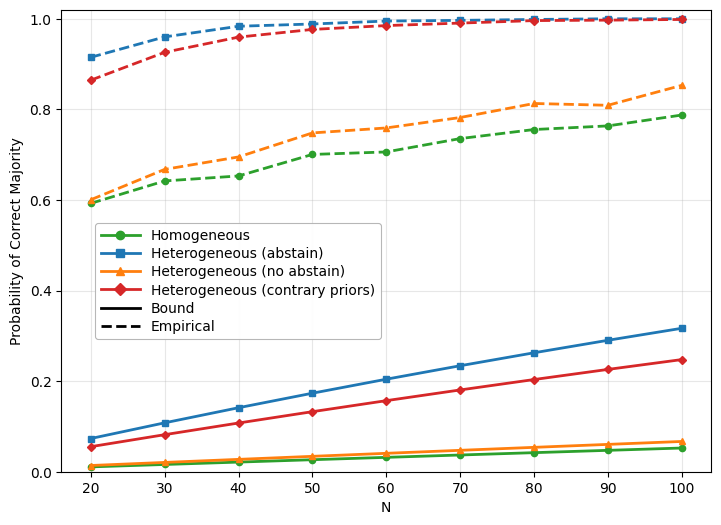
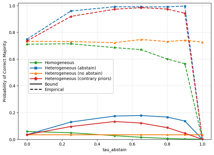
In this subsection, we empirically assess the bound from Theorem 1 by Monte Carlo simulation of the full process, and compare this to the Azuma–Hoeffding lower bound (Equation 2) computed from the same parameters. For a pseudocode description of the implementation, we refer the reader to subsection 5.5 of the appendix. In each simulation round we: (i) draw all private outcomes for all agents over the learning tasks; (ii) update each agent’s Beta counts; (iii) apply the gate at time using and ; (iv) sample each publishing agent’s final private vote on ; and (v) record whether the final majority is correct. Repeating this times yields the empirical success probability (the share of rounds in which the correct alternative wins). We consider four agent pools, accounting for different competence distributions, and their interaction with the abstention gate, across two parameter configurations. That is, (i) Homogeneous agents (identical competencies); (ii) Heterogeneous agents with a prescribed -value, and uniform Beta priors (); (iii) Heterogeneous agents that never abstain () as a baseline comparison; (iv) Heterogeneous agents with priors chosen contrary to their true reliability. That is, setting (iv) studies miscalibrated Beta priors, implemented as follows: For agent with true reliability , choose a prior strength (total pseudo–count) and set (for to ensure for numerical stability): That is, competent agents () start pessimistic, and incompetent agents () start optimistic. For all settings, we assume an average reliability of , trials, and . Heterogeneity is implemented by assigning to equal-sized halves, so that .
In Figure 3(a), we plot the bound and empirical success probability as the number of agents () varies, prescribing for all agents. In Figure 3(b), we plot against a common for agents. Across both settings, the gated models (blue: heterogeneous with uniform priors; red: heterogeneous with contrary priors) dominate the non-abstaining baseline (orange) and the homogeneous pool (green): selective abstention suppresses low-competence voters, so the publishing electorate is, in expectation, stronger, leading to both a higher empirical success rate, and theoretical minimum success probability. An exception appears in Fig. 3(b) for very large gates: once exceeds what even the better half () can typically certify, many agents stop publishing and performance degrades, while the non-abstaining baseline remains roughly flat. In both plots, the empirical success rates (dashed) lie well above the theoretical curves (solid). This is expected as Equation˜2 is a worst-case concentration bound, protecting against the most unfavorable realizations by only using coarse information about the process.
5 Summary and Future Work
In this work, we introduced a probabilistic framework to analyze collective decision-making with endogenous participation. By employing martingales and filtrations, we captured the dynamic evolution of agents’ confidence and their resulting decision to vote or abstain. Our primary contribution is the derivation of a non-asymptotic lower bound on the probability of a correct majority, alongside an asymptotic guarantee that extends the classical CJT to settings with heterogeneous agents and confidence-based abstention.
This framework offers a theoretical bridge between two distinct views on abstention: the strategic view of social choice theory (where agents abstain to avoid pivoting the vote incorrectly) and the epistemic view of statistical learning (where agents abstain due to low confidence). We showed that “calibrated” agents who simply maximize their own precision naturally improve the collective information state.
For future work, we plan to explore three avenues. First, from a theoretical standpoint, we aim to derive tighter concentration bounds by incorporating the variance structure of the martingale difference sequence (e.g., using Freedman’s inequality). Second, regarding social choice axioms, we wish to relax the independence assumption to model correlated information sources, a common scenario in committee deliberations. Finally, we plan to apply this framework to the design of hybrid intelligence systems, using Large Language Models (LLMs) as calibrated agents to empirically validate how confidence-gated voting mitigates group-level hallucination in collective decision-making. This will involve: (i) instantiating the agents as individual LLMs or as different reasoning paths of a single LLM, (ii) using a feedback loop to simulate the learning process and update their competence beliefs, and (iii) evaluating the success of our confidence-based abstention mechanism in mitigating hallucinations on a range of binary decision tasks.
Appendix
5.1 Proof for Proposition 1.
We verify that forms a martingale difference sequence with respect to the filtration . Recall that we let
be the centered random variable representing the total deviation of interest and that we can then construct a Doob martingale for this centered variable:
Each represents the change in the conditional expectation of the centered sum of final votes when the -th private outcome is revealed.
We show each property individually.
1. Integrability (): By the triangle inequality, . Recall that . The random variable is a sum of terms (agents’ votes at time ), each bounded within . Thus, is bounded within . Consequently, the centered variable is also bounded. Specifically, its values lie within . Since is itself bounded within , the range of the centered variable is at most . The conditional expectations and are therefore also bounded random variables. A bounded random variable has a finite expected absolute value. Consequently, is finite.
2. Adaptedness ( is measurable with respect to ):
A random variable is said to be -measurable if, for every Borel set in the measurable space , where refers to the collection of all subsets of that satisfy the properties of a -algebra (containing the empty set and , and being closed under complementation and countable unions), and thus are precisely the sets to which a probability measure can be consistently assigned, the preimage is an element of the -algebra [9]. In essence, this means that for any possible value or range of values that can take, we can determine, solely by observing the events in , whether falls into that value or range.
In our specific context, the random variables and (and thus ) take on values that are conditional expectations of the centered variable . A key property of conditional expectation is that is always -measurable for any random variable for which the expectation exists [9].
Let’s demonstrate why is -measurable. For to be -measurable, both and must be -measurable.
-
•
Measurability of with respect to : By the very definition of a Doob martingale, is, by construction, -measurable. Therefore, for any Borel set , the event is an element of .
-
•
Measurability of with respect to : The random variable is, by definition, -measurable. Since is a filtration, it satisfies the property that . This implies that any random variable that is measurable with respect to the smaller -algebra is also measurable with respect to the larger -algebra . This is the case since for every Borel set , it holds that if , then . Therefore, is -measurable.
Since both and are -measurable random variables, their difference, , is also -measurable. This follows from the fact that for any two measurable functions, their difference is also measurable [26]. This confirms that the sequence is adapted to the filtration .
3. Zero Conditional Mean (): We expand :
| (By linearity of conditional expectation) | |||
Since is measurable with respect to (i.e., known given ), . For the first term, by the tower property of conditional expectation ( for any random variable given that the filtration is ordered sequentially):
Substituting these back, we find:
Thus, all three conditions are satisfied, confirming that is indeed a martingale difference sequence with respect to .
5.2 Proof for Lemma 2.
Recall that we let
be the centered random variable representing the total deviation of interest and that we can then construct a Doob martingale for this centered variable:
Each represents the change in the conditional expectation of the centered sum of final votes when the -th private outcome is revealed.
As a general strategy to determine for , we determine the maximal change in expectation we can obtain from a single martingale difference. More specifically, we consider a specific but arbitrarily chosen event in the event-based filtration and take into account the time of its occurrence.
Let denote the specific agent and time step corresponding to the -th private outcome, . The filtration contains all information in plus the outcome of .
The variable is the conditional expectation of . When is revealed, it only affects the conditional expectation of (and consequently the term ). The conditional expectations of other agents’ votes (for ) are independent of given and thus their contribution to the change is zero. Thus, the martingale difference simplifies to:
Since is a constant, i.e. an unconditional expectation (which we can denote as ), and recalling the linearity property of conditional expectation () and that the conditional expectation of a constant is the constant itself (), we can expand the terms:
The individual net public vote for agent at time is bounded within . Consequently, any conditional expectation of must also lie within the range .
We now establish the bounds for based on the time step of the revealed outcome :
-
1.
If corresponds to agent at time : In this case, is a private choice made by agent at a time step prior to the final vote. We have . The term represents agent ’s private choice at time . By our distribution-level reliability assumption, private choices are independent across trials. This means is independent of all past private outcomes (including and the entire filtration ) and (which is determined by prior information), since the distribution of depends only on (here ) and not on past history. Therefore, we can write:
Since is independent of all past outcomes which determine and , the inner expectation simplifies to: Then, as is a constant, it can be factored out of the outer expectation. Here, we made use of the Tower Property of Conditional Expectation. This property states that for any random variable and nested -algebras :
In our derivation, is the product . We set and choose . This specific choice of is made to ensure that is measurable with respect to the inner conditioning set, allowing it to be factored out from the inner expectation.
The same logic applies to . Substituting these into the expression for :
The terms and are conditional probabilities of (a binary variable that is or ). Thus, they both lie in the interval . The maximum possible absolute difference between any two values in this interval is . Therefore, . We set . Note that .
-
2.
If corresponds to agent at time : In this scenario, is , the actual private choice of agent at the final time step . When this outcome is revealed at step , it directly determines the value of for agent (since is already determined by information up to time , making it -measurable). Specifically:
-
•
For we obtain: , because (and thus ) is now known given .
-
•
For we obtain:
This holds because is -measurable, and is independent of by the independence of task from past tasks.
Thus,
Substituting :
We consider the two possible values of :
-
•
If , then , so holds.
-
•
If , then . Since and :
-
–
If , .
-
–
If , .
The maximum absolute value of these terms is , which occurs at or , and is equal to . Thus, .
-
–
We set .
-
•
Now, we calculate the sum of squares of these bounds over all events. We can group terms based on whether the private outcome occurred before time () or at time (). Let be the set of indices where the corresponding time , and be the set of indices where the corresponding time .
For , we established that the bound . There are time steps (from to ) for each of the agents where this case applies. So, there are such terms. For , we established that the bound . This case applies for each of the agents at the final time step . So, there are such terms.
The sum of squares of these bounds over all events is therefore:
Substituting the derived bounds for :
In the first sum, for each agent , the term appears times (once for each time step from to ). In the second sum, for each agent , the term appears once (for the final time step ). This simplifies to:
5.3 Proof for the Hallucination Bound.
In this proof, we utilize the upper-tail variant of the Azuma-Hoeffding inequality, restating Lemma 1 from above [2]:
Let be a martingale difference sequence w.r.t. with a.s. for all . Then, for any ,
For this derivation, we condition on . From Lemma 1 and Lemma 2, we obtain the following derivation:
| We subtract from both sides. | ||||
| Apply the (upper-tail) Azuma–Hoeffding bound with , , | ||||
| and . | ||||
| Substitute the expected total net public vote under : | ||||
| (4) |
5.4 Proof for Theorem 3.
As before, we condition on the final task’s true state and write and accordingly. Recall the one-sided Azuma–Hoeffding lower bound derived in Equation 2. We seek to show that as , the probability of a correct majority converges to 1.
We recall the underlying parameters: is the final net vote, is agent ’s distribution-level reliability, and is the publication decision. The term represents the agent’s expected margin.
Let be the number of learning rounds. The agent’s decision to publish at time depends on the number of correct predictions observed during learning.
To prove convergence, we proceed in four steps:
(i) establish that the number of successes follows a Binomial distribution; (ii) show that the confidence is non-decreasing in , implying the publish rule is a success-count threshold; (iii) bound the expected publish probability and vote margin using the uniform non-degeneracy assumption; (iv) apply these bounds to the Azuma-Hoeffding result to show exponential convergence.
Step 1: Distribution of Successes. Under the distribution-level reliability definition, the outcomes of the learning tasks are i.i.d. Bernoulli() trials. Thus, for any agent , the success count follows a binomial distribution:
Step 2: Monotonicity and Threshold Rule. After observing successes, the posterior is . The agent publishes if its confidence exceeds . For a fixed critical threshold , the regularized incomplete beta function is decreasing in and increasing in . Since observing more successes () increases and decreases , the tail probability is strictly non-decreasing in .
Consequently, the condition defines a success-count threshold: there exists some such that the agent publishes if and only if .
Step 3: Bounding the Publish Probability.
We define the publish probability for agent as a function of their competence :
Lemma 3 (Convergence).
Fix the horizon and the gate parameters (). Consider a sequence of agents satisfying two conditions:
-
1.
Average Competence: The average reliability exceeds by a margin :
-
2.
Uniform Non-degeneracy: The gate is uniformly nondegenerate, meaning there exists a lower bound such that for all agents and all , the probability of publishing is at least (i.e., for competent agents).
Then, as ,
| (5) |
Proof.
Recall the exponent from the Azuma-Hoeffding lower bound (Eq. 2). We analyze the numerator and denominator separately.
Denominator: The variance term for each agent is bounded by . Summing over agents:
Numerator: The expected collective vote is . Note that . We split the sum into competent () and incompetent () agents. For incompetent agents, , so their contribution to the sum is negative (or zero). For competent agents, we use the uniform non-degeneracy assumption: . Thus:
| (Since and terms are negative, replacing with 1 lowers the sum) | |||
| (Assuming , we can factor it out safely) | |||
Using the average competence assumption , we get:
Step 4: Convergence.
Substituting these into the Azuma-Hoeffding bound:
Since and is finite, the exponent grows linearly with , driving the error probability to 0. ∎
5.5 Pseudocode for Empirical Evaluation.
We evaluate the framework using three routines: a per–agent gate-and-contribution calculator (Alg. 1), a lower bound aggregator (Alg. 2), and a Monte–Carlo simulator of the full sequential process (Alg. 3).
We vary a single control parameter (e.g. , , ) while keeping the others fixed, and report four scenarios: (i) homogeneous agents (); (ii) heterogeneous with abstention (half , half ); (iii) the same heterogeneous pool with abstention disabled; and (iv) heterogeneous with contrary (competence-inverse) priors used during learning. For each setting we plot the probabilistic lower bound from Algs. 1–2 alongside the Monte–Carlo estimate from Alg. 3. Consistently, the gate filters low-competence agents, increasing the expected margin and tightening the lower bound; both empirical success and the certificate improve with larger and .
Contrary priors (used in scenario (iv)).
For agent with true reliability , we set the Beta prior mean to with strength , and we clip Beta pseudo–counts below by to ensure for numerical stability:
so competent agents start pessimistic and weak agents optimistic. (When not using contrary priors we employ aligned, shared priors for all agents.) For instance, with and a competent agent , we set
so the prior is pessimistic despite . Conversely, for a weak agent ,
yielding an optimistic prior .
Alg. 1 (AgentGateAndContribution). Fix horizon (with learning rounds), agent ’s prior (aligned or contrary), competence , target level , and abstention threshold . The routine enumerates all learning histories with correct private outcomes. For each it forms the posterior and computes the agent’s confidence . If (or if publishing is forced), that history counts as “publish”. Weighting by the binomial likelihood and summing over yields , the probability that agent will publish at time under the model. Multiplying by the margin gives the agent’s expected contribution to the final net vote. The update implements the law of total probability:
that is, we add the probability of each history that would vote publicly.
Alg. 2 (BoundFromContrib). Given the per–agent contributions and competences , the routine computes the numerator and the Azuma–Hoeffding denominator , which collects the bounded differences from the learning reveals and the final private vote (Lemma 2). It returns the lower bound on the probability that the final majority is correct.
Alg. 3 (MonteCarloEvaluate). This routine simulates the full process end-to-end. In each run it initializes all agents with either a shared prior or per–agent priors (e.g., contrary priors as above), then executes learning rounds. In round , agent draws a private outcome (correct with probability ) and updates its Beta counts accordingly. At the decision round , each agent computes its posterior confidence and publishes iff it exceeds (or publishing is forced). Publishing agents then cast a final private vote ( w.p. , otherwise). The net vote is the sum of published votes; a run is a win if the net number of votes is strictly positive. Repeating over runs yields the empirical success rate, referred to as .
References
- [1] (2022) How should we vote? a comparison of voting systems within social networks.. In IJCAI, pp. 31–38. Cited by: §1.2.
- [2] (1967) Weighted sums of certain dependent random variables. Tohoku Mathematical Journal, Second Series 19 (3), pp. 357–367. Cited by: §5.3, Lemma 1.
- [3] (1989) Modelling dependence in simple and indirect majority systems. Journal of Applied Probability 26 (1), pp. 81–88. External Links: ISSN 00219002, Link Cited by: §1.2.
- [4] (1996) Bagging predictors. Machine learning 24 (2), pp. 123–140. Cited by: §1.
- [5] (1957) An optimum character recognition system using decision functions. IRE Transactions on Electronic Computers EC-6 (4), pp. 247–254. External Links: Document Cited by: §1.3.
- [6] (1785) Essai sur l’application de l’analyse à la probabilité des décisions rendues à la pluralité des voix. Imprimerie Royale, Paris. Cited by: §1, §1.
- [7] (2000) Ensemble methods in machine learning. In Multiple Classifier Systems, Berlin, Heidelberg, pp. 1–15. External Links: ISBN 978-3-540-45014-6 Cited by: §1.
- [8] (2001) Elements of martingale theory. In Classical Potential Theory and Its Probabilistic Counterpart, External Links: ISBN 978-3-642-56573-1, Document, Link Cited by: Definition 7.
- [9] (2019) Probability: theory and examples. Vol. 49, Cambridge university press. Cited by: §3, §3, §5.1, §5.1, Definition 2.
- [10] (2010) The epistemic view of belief merging: Can we track the truth?. In Proceedings of the 19th European Conference on Artificial Intelligence (ECAI 2010), H. Coelho, R. Studer, and M. J. Wooldridge (Eds.), FAIA, Vol. 215, pp. 621–626. External Links: Link, Document Cited by: §1.2, §1.
- [11] (2019) Selectivenet: a deep neural network with an integrated reject option. In International conference on machine learning, pp. 2151–2159. Cited by: §1.3.
- [12] (1990) Neural network ensembles. IEEE transactions on pattern analysis and machine intelligence 12 (10), pp. 993–1001. Cited by: §1.
- [13] (2022) Language models (mostly) know what they know. External Links: 2207.05221, Link Cited by: §1.3.
- [14] (2021) Liquid democracy: an algorithmic perspective. Journal of Artificial Intelligence Research 70, pp. 1223–1252. Cited by: §1.2.
- [15] (2025) Why language models hallucinate. External Links: 2509.04664, Link Cited by: §1.3, §4.
- [16] (2024) To lead or to be led: a generalized condorcet jury theorem under dependence. In Proceedings of the 23rd International Conference on Autonomous Agents and Multiagent Systems, pp. 983–991. Cited by: §2, §2, §3.
- [17] (1999) Merging with integrity constraints. In European Conference on Symbolic and Quantitative Approaches to Reasoning and Uncertainty, pp. 233–244. Cited by: §1.
- [18] (1992) The Condorcet jury theorem, free speech, and correlated votes. American Journal of Political Science 36 (3), pp. 617–634. External Links: ISSN 00925853, 15405907, Link Cited by: §1.2.
- [19] (2000) Classifier combinations: implementations and theoretical issues. In Proceedings of the First International Workshop on Multiple Classifier Systems (MCS 2000), J. Kittler and F. Roli (Eds.), LNCS, Vol. 1857, pp. 77–86. External Links: Link, Document Cited by: §1.
- [20] (1990) A statistical approach to learning and generalization in layered neural networks. Proceedings of the IEEE 78 (10), pp. 1568–1574. Cited by: §1.
- [21] (2001) Epistemic democracy: generalizing the Condorcet jury theorem. Journal of Political Philosophy 9 (3), pp. 277–306. External Links: Document, Link, https://onlinelibrary.wiley.com/doi/pdf/10.1111/1467-9760.00128 Cited by: §1.2.
- [22] (2002) Aggregating sets of judgments: an impossibility result. Economics & Philosophy 18 (1), pp. 89–110. Cited by: §1.
- [23] (2018) Complete convergence and complete moment convergence for randomly weighted sums of martingale difference sequence. Journal of Inequalities and Applications 2018, pp. 1–16. Cited by: §3.
- [24] (1989) Proving a distribution-free generalization of the Condorcet Jury Theorem. Mathematical Social Sciences 17 (1), pp. 1–16. External Links: Document, Link Cited by: §1.2.
- [25] (2017) Epistemic democracy with correlated voters. Journal of Mathematical Economics 72 (C), pp. 51–69. External Links: Document, Link Cited by: §1.2.
- [26] (2016) Measure and integration. European Mathematical Society. Cited by: §5.1.
- [27] (1990) The design and analysis of efficient learning algorithms. Ph. D. Thesis. MIT. Cited by: §1.
- [28] (2024) Truth-tracking with non-expert information sources. Journal of Artificial Intelligence Research 81, pp. 619–641. Cited by: §1.
- [29] (2012) Courts of many minds. British Journal of Political Science 42 (3), pp. 555–571. External Links: ISSN 00071234, 14692112, Link Cited by: §1.2.
- [30] (2023) Cjt-deo: condorcet’s jury theorem and differential evolution optimization based ensemble of deep neural networks for pulmonary and colorectal cancer classification. Applied Soft Computing 132, pp. 109872. Cited by: §1.
- [31] (2022) Ensemble of deep neural networks based on condorcet’s jury theorem for screening covid-19 and pneumonia from radiograph images. Computers in Biology and Medicine 149, pp. 105979. Cited by: §1.
- [32] (2023) Self-consistency improves chain of thought reasoning in language models. External Links: 2203.11171, Link Cited by: §1.3.