Enabling clinical use of foundation models in histopathology
Audun L. Henriksen1*,
Ole-Johan Skrede1*,
Lisa van der Schee2,
Enric Domingo3,4,
Sepp De Raedt1,
Ilyá Kostolomov1,
Jennifer Hay5,
Karolina Cyll1,
Wanja Kildal1,
Joakim Kalsnes1,
Robert W. Williams6,
Manohar Pradhan1,
John Arne Nesheim1,
Hanne A. Askautrud1,
Maria X. Isaksen1,
Karmele Saez de Gordoa7,8,9,
Miriam Cuatrecasas7,8,9,
Joanne Edwards10,
TransSCOT group‡,
Arild Nesbakken11,12,
Neil A. Shepherd13,
Ian Tomlinson3,
Daniel-Christoph Wagner14,
Rachel S. Kerr3,
Tarjei Sveinsgjerd Hveem1,
Knut Liestøl1,
Yoshiaki Nakamura3,15,16,
Marco Novelli17,
Masaaki Miyo18,
Sebastian Foersch14,
David N. Church19,20,
Miangela M. Lacle2,
David J. Kerr21,
Andreas Kleppe†1,22,23
1Institute for Cancer Genetics and Informatics, Oslo University Hospital, Oslo, Norway
2Department of Pathology, University Medical Center Utrecht, Utrecht, The Netherlands
3Department of Oncology, University of Oxford, Oxford, UK
4CRUK Beatson Institute of Cancer Research, Garscube Estate, Glasgow, UK
5Glasgow Tissue Research Facility, University of Glasgow, Queen Elizabeth University Hospital, Glasgow, UK
6Area for Improvement and Digital Transformation, Norwegian Offshore Directorate, Stavanger, Norway
7Pathology Department, Hospital Clínic, Barcelona, Spain
8Institut d’Investigacions Biomèdiques August Pi I Sunyer (IDIBAPS), Barcelona, Spain
9Department of Clinical Foundations, Universitat de Barcelona, Barcelona, Spain
10School of Cancer Sciences, Wolfson Wohl Cancer Research Centre, University of Glasgow, Glasgow, UK
11Institute of Clinical Medicine, University of Oslo, Oslo, Norway
12Department of Gastrointestinal Surgery, Oslo University Hospital, Oslo, Norway
13Gloucestershire Cellular Pathology Laboratory, Cheltenham General Hospital, Cheltenham, UK
14Institute of Pathology, University Medical Center, Mainz, Germany
15Department of Gastrointestinal Oncology, National Cancer Center Hospital East, Kashiwa, Japan
16Translational Research Support Office, National Cancer Center Hospital East, Kashiwa, Japan
17Department of Cancer Biology and Pathology, University College London, London, UK
18Department of Gastroenterological Surgery, Osaka International Cancer Institute, Osaka, Japan
19Centre for Human Genetics, University of Oxford, Oxford, UK
20Oxford NIHR Comprehensive Biomedical Research Centre, Oxford University Hospitals NHS Foundation Trust, John Radcliffe Hospital, Oxford, UK
21Nuffield Division of Clinical Laboratory Sciences, University of Oxford, Oxford, UK
22Department of Informatics, University of Oslo, Oslo, Norway
23Centre for Research-based Innovation Visual Intelligence, UiT The Arctic University of Norway, Tromsø, Norway
*Joint first authors with equal contribution.
†Corresponding author:
Andreas Kleppe
Institute for Cancer Genetics and Informatics, Oslo University Hospital
NO-0424 Oslo, Norway
andrekle@ifi.uio.no
‡The individual names of the TransSCOT Trial Management Group are listed in the Appendix to the main manuscript, and the individuals should be listed as collaborators.
Abstract
Foundation models in histopathology are expected to facilitate the development of high-performing and generalisable deep learning systems. However, current models capture not only biologically relevant features, but also pre-analytic and scanner-specific variation that bias the predictions of task-specific models trained from the foundation model features. Here we show that introducing novel robustness losses during training of downstream task-specific models reduces sensitivity to technical variability. A purpose-designed comprehensive experimentation setup with 27,042 WSIs from 6155 patients is used to train thousands of models from the features of eight popular foundation models for computational pathology. In addition to a substantial improvement in robustness, we observe that prediction accuracy improves by focusing on biologically relevant features. Our approach successfully mitigates robustness issues of foundation models for computational pathology without retraining the foundation models themselves, enabling development of robust computational pathology models applicable to real-world data in routine clinical practice.
Introduction
Inspired by the success of foundation models in natural language processing, several pathology foundation models have been published in recent years.[bommasani2021opportunities, chen2024towards, xu2024whole, zimmermann2024virchow2, filiot2024phikon, nechaev2024hibou] These models are trained in a self-supervised manner on large and diverse collections of whole-slide images (WSIs), with the aim of serving as general-purpose feature extractors for downstream tasks such as tissue classification, biomarker prediction, and survival analysis.[chen2024towards, zimmermann2024virchow2, filiot2024phikon, nechaev2024hibou] They are assumed to produce more robust and generalisable downstream models, which is critical for the adoption of computational pathology models in routine clinical practice.[Kleppe2021DesigningDL, vanderLaak2021DeepLI]
Deep learning models do not inherently distinguish biologically meaningful features from spurious correlations present in training data. Consequently, they can exploit such correlations to optimise the training function, a phenomenon called shortcut learning.[geirhos2020] In medical imaging, this is a prominent issue because differences in procedures and devices between centres make it particularly easy for models to exploit medically irrelevant patterns that will not generalise to new data. Well-known examples include rulers or surgical markings present in dermatological photographs, [narla2018, winkler2019association] radiographic markers in X-ray images,[zech2018], and institutional signatures embedded in histological images.[howard2021, dehkharghanian2023, Clusmann2025IncidentalPI] In histopathology, additional domain-specific sources of variation further contribute to this problem. Pre-analytic factors related to tissue processing, [howard2021, kheiri2025] staining reagents, [tellez2019, lin2025] and digital scanning equipment,[stacke2019, aubreville2023, thiringer2026] can introduce substantial non-biological variation into WSIs, and deep learning models have been shown to be sensitive to these technical aspects[tellez2019, lin2025, stacke2019, aubreville2023, thiringer2026, howard2021, kheiri2025].
Despite being trained on large and diverse datasets, foundation models have recently been shown to lack robustness to technical variation. Studies evaluating robustness of multiple pathology foundation models have reported that their features encode attributes of the medical centre and scanner more prominently than underlying biological features, regardless of training data scale or model size.[dejong2025, thiringer2026] The features have high slide-level dependence but low disease-level specificity, and stain normalisation, a common technique for standardising the colour appearance of WSIs, does not remove the slide-related dependence.[mishra2025, komen2024]
A common task in computational pathology is the classification of WSIs where ground-truth labels are available only for the entire WSIs. Features of image subregions (called tiles) of the WSIs are often computed from foundation models and processed by a few fully-connected layers before being pooled and used to make a prediction for the WSIs. In this conventional setting, Carloni et al.[carloni2025] proposed to utilise a second set of training data, containing WSIs of the same section imaged on different scanners, and include a loss term that penalise discrepancies between the tile feature in order to reduce scanner-related dependence. Because the tiles in the ordinary set of training data were processed by the same subnetwork in their pipeline, the resulting tile features should be less dependent on the particular scanner. They showed that applying this pipeline makes the WSI predictions less scanner dependent and observed an increased robustness of 21% when training using two WSIs of the same sections and 34% when training using six WSIs of the same sections, in an experiment using 3405 WSIs to predict Epidermal Growth Factor Receptor (EGFR) mutation in lung cancer.[carloni2025]
Rather than applying separate data to improve robustness only in tile features, we propose that the robustness of the WSI prediction may be further improved by regularising the entire downstream task-specific network through training with multiple robustness losses for a single set of data consisting of co-registered tiles from two or more scanners. Specifically, we introduce two loss terms to the standard approach that encourage the model to produce consistent outputs for the same tissue region imaged on different scanners. These losses are applied only during training and do not modify the underlying foundation model or the architecture of the downstream task-specific network, implying that the downstream models trained with this approach can be applied to classify individual WSIs imaged on only one scanner, thus making it compatible with the anticipated use of computational pathology models in routine clinical practice.
We demonstrate the utility of this regularisation approach through extensive experimentation with eight popular foundation models for computational pathology and two clinical tasks; survival outcome prediction in early-stage colorectal cancer (CRC) and lymph node metastasis (LNM) prediction in pathological T1 (pT1) CRC. Multiple WSIs of the same hematoxylin and eosin (H&E)-stained tissue section scanned on different scanners were included, as well as different tissue sections of the same tumour that were prepared and imaged in different laboratories. In total, the experimentation setup comprised 27,042 WSIs from 6,155 patients, which were used to train and externally test thousands of downstream task-specific models based on systematic tuning of about 350,000 models. We show that the proposed regularisation substantially improves robustness to scanner variation across all eight foundation models and also improves prediction accuracy through focusing on biologically relevant features.
Results
Foundation models in histopathology are sensitive to non-biological differences
Features from 7777 WSIs from 2250 patients were extracted using published foundation models. First, we use these features to train and tune deep learning models for CRC survival outcome prediction using a common attention-based multiple instance learning approach (Fig. 1a)[ilse2018attention]. To test the robustness to sample preparation and imaging variation of the resulting models, we analysed two tissue slides from each of 2875 patients from TransSCOT, the translational arm of the SCOT trial[Iveson20183V6]. For each patient, one slide consisted of a 4 µm thick section that was sectioned, stained and imaged in UK (hereafter named ‘original slide’), while the other consisted of a 5 µm thick section that was stained and imaged on five different pathology scanners in Norway (Fig. 2a,b).
Mapping the high-dimensional features from a foundation model into two-dimensional points with t-distributed stochastic neighbour embedding (t-SNE)[van2008visualizing] and labelling them with the source of origin clearly shows that the foundation model features cluster WSIs primarily by origin and not biological differences (Fig. 2c). Comparison of prediction scores produced by the conventionally trained models for different WSIs of the same patient showed substantial variability related to the laboratory site and scanner device for all foundation models (Fig. 2d and Extended Data Fig. 1). Thus, the predictions generated by conventionally trained downstream task-specific models inadvertently apply non-biological information contained in the features from foundation models, resulting in patient representations that are suboptimal for the intended prediction task.
By quantifying robustness as the relative average standard deviation of the prediction score for different WSIs from the same patient, referred to as the inconsistency metric (see Methods for more details), we find that the inconsistency varies between foundation models as well as between individual training runs using features from the foundation model (Fig. 3b). Hibou-L and Phikon-v2 show the highest average inconsistency of 0.52 and 0.45, respectively. Prov-GigaPath, Virchow2, H-Optimus 0 and 1, UNI, and UNI2 display lower inconsistency, with an average value of around 0.25.
After dichotomising the prediction scores into classifications of patient outcome by selecting the class with highest score, we measure the percentage of agreement in classification between each pair of different WSIs from the same patient. Models trained on Hibou-L features have an average classification agreement of about 80%, Phikon-v2 models have about 86%, and models trained on features from one of the other six foundation models have between 90% and 93% (Fig. 3c).
Generalisation of scanner information in foundation model features
To investigate the congruity across datasets for the scanner information contained within the foundation model features, we train a simple linear classifier to classify the originating scanner directly from the foundation model features using the QUASAR 2 dataset and externally test the classifier on the TransSCOT dataset. This linear probing shows that all five scanners can be accurately identified across datasets, with an average classification accuracy in the external test dataset of 1.000 for Phikon-v2, above 0.998 for H-Optimus-0, H-Optimus-1, UNI, UNI2, and Virchow2, 0.992 for Prov-GigaPath, and 0.986 for Hibou-L (see Extended Data Fig. 2). This shows that the foundation models represent non-biological information consistently across patients and sample preparations, thus supporting how prominent these attributes are in the foundation model features.
Training robust downstream task-specific models from foundation model features
To encourage similar predictions for different WSIs of the same tissue section, we include two additional loss terms; a contrastive loss on tile-level embeddings, based on InfoNCE[oord2018], that pulls together features of the same physical area imaged on different scanners while pushing apart features from different patients, and a mean squared error loss on the prediction scores that penalises differences in the final slide-level predictions between corresponding WSIs (Fig. 1b). Each of these loss terms is multiplied with a weight factor and added to the ordinary classification loss to define the full loss function.
With these additional loss terms, we train and tune downstream task-specific models to predict survival outcome using the foundation model features that were previously extracted from 7777 WSIs from 2250 patients (Fig. 3a). The prediction scores of the resulting models for different WSIs from the same patient in the TransSCOT test dataset are notably more similar (Fig. 2e and Extended Data Fig. 1) than without the robustness losses (Fig. 2d and Extended Data Fig. 1). In terms of average inconsistency, it improves to below 0.2 for all foundation models and to below 0.1 for all except Hibou-L and Phikon-v2 (Fig. 3b). Compared to the conventionally trained downstream task-specific models, the consistency improvement is statistically significant for all foundation models (p ¡ 0.001) and ranged from 177% to 259% (Extended Data Table 1). We also observe a substantial increase for average classification agreement, and again applying the most robust foundation model without the robustness loss gives worse robustness than applying the least robust foundation model with robustness loss (Fig. 3b). The average classification agreement was above 95% for all foundation models except Phikon-v2 and Hibou-L. Compared to the default setting without any additional loss terms, we see a statistically significant improvement in classification agreement for all foundation models (p ¡ 0.001), with a relative improvement between 111% and 209% (Extended Data Table 1).
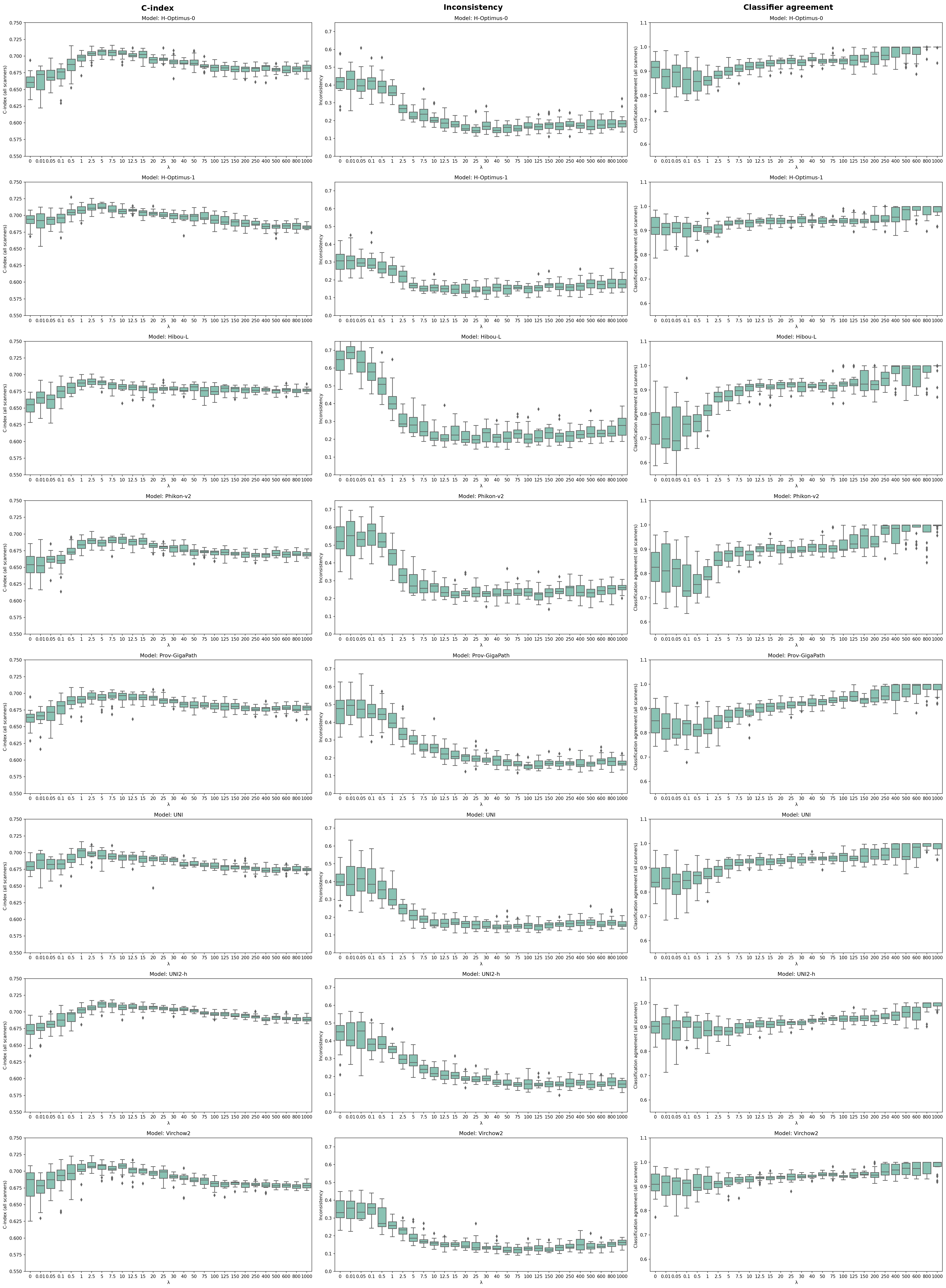
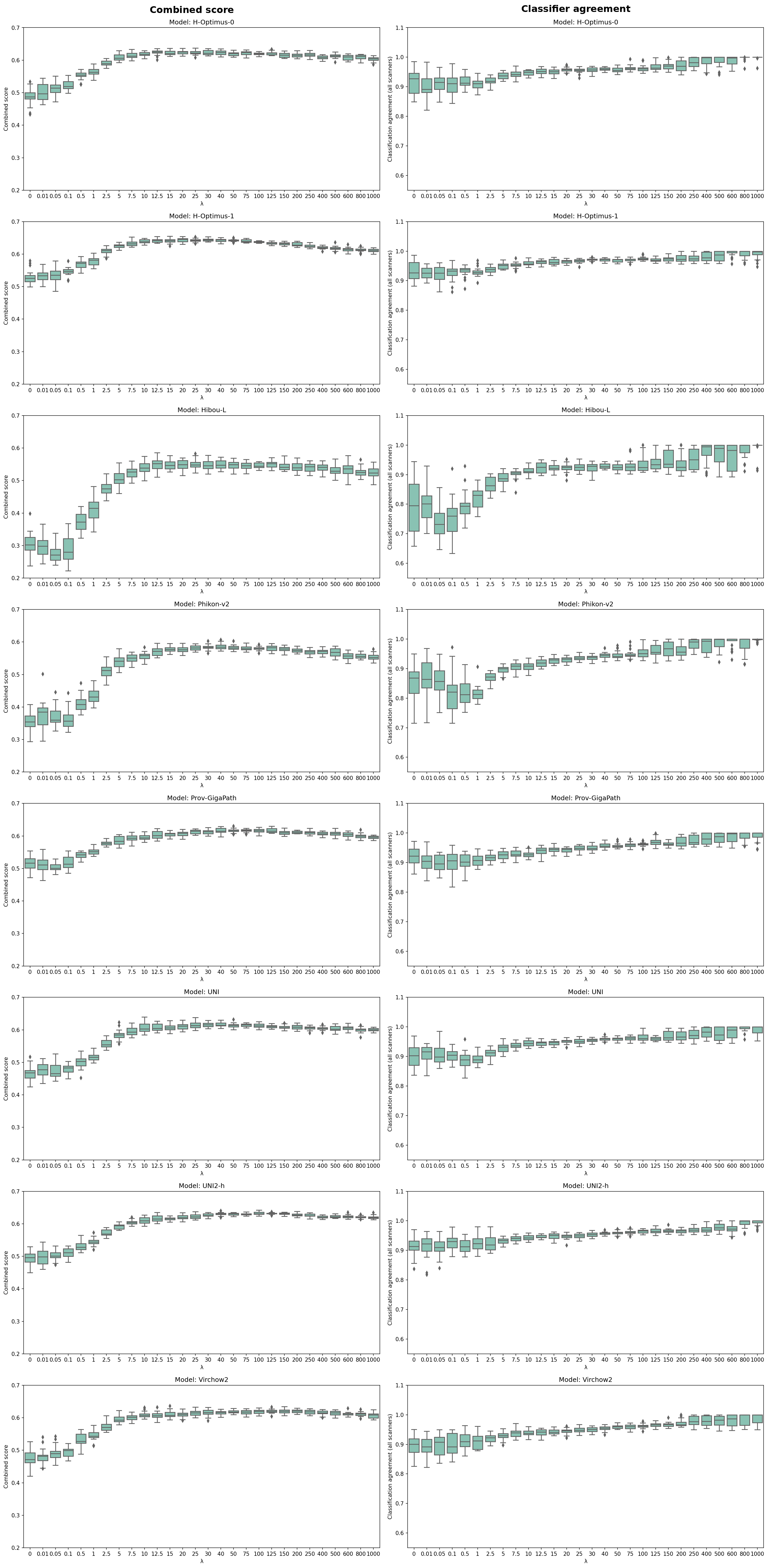
The balance between robustness and prediction accuracy is controlled by the weight factor that scales the robustness losses. To prevent reduced predictive accuracy at excessively high weights (Extended Data Fig. 3), foundation model-specific weights were determined by optimising a score combining inconsistency and c-index in the tuning dataset (Extended Data Fig. 4; see Methods for more details). For this selection of weight, the downstream task-specific models are both more robust and have similar or better prediction accuracy in terms of c-index in external test data (Fig. 3b). Gradually increasing the weight from 0 confirms this initial increase in both robustness and prediction accuracy when introducing the robustness losses (Extended Data Fig. 3). Consequently, the combined score balancing robustness and prediction accuracy is significantly better with robustness loss for all foundation models (p ¡ 0.001; Fig. 3b).
Congruity of spatially resolved predictions
The consistency of the prediction score for different WSIs from the same patients (Fig. 4a) indicates that the downstream task-specific model learns to ignore the information in the foundation model features that captures non-biological information related to sample preparation and scanner device. If this is true, then applying downstream task-specific models to the individual image tiles should also be much more consistent when the model is trained with and without robustness loss. Using a representative patient from the test dataset, the heatmaps of the prediction scores for individual tiles demonstrate superior consistency between WSIs from the same patient when training the model with robustness loss (Fig. 4b).
Analyses of each layer in the downstream task-specific models
To understand where in the downstream task-specific models the robustness terms introduce changes, we analyse each layer of the best individual model in the QUASAR 2 tuning dataset for each foundation model. First, we compute the cosine similarity between WSIs from the same patient and find that it is statistically significantly larger in each layer of the downstream task-specific models (Fig. 5). This shows that already the first layer of the downstream task-specific models learns to focus on biologically meaningfull information contained in the foundation model features, but the similarity between WSIs from the same patient also increases by each subsequently layer of the model (Fig. 5). When instead analysing the cosine similarity between WSIs from different patients that were prepared at the same laboratory and using the same scanner, we find that the features from models trained with robustness loss have statistically significant lower similarity (Fig. 5). This indicates that different patients are more clearly separated by the features from the models trained with robustness loss than those from the models trained without robustness loss, which suggests that the unique biology of each patient is more distinctly and better characterised when applying the robustness losses during training.
Replication in different prediction task
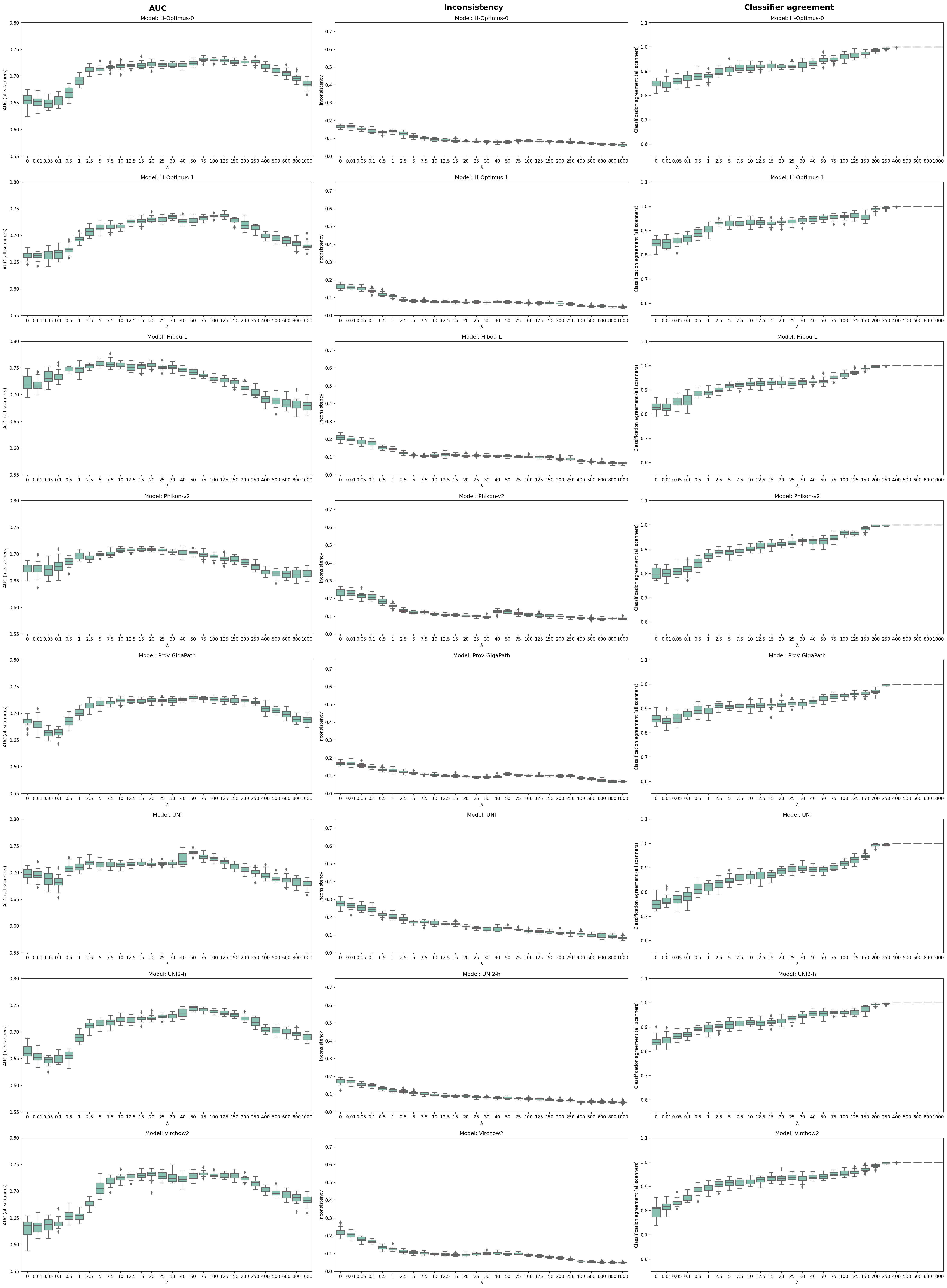
In order to demonstrate that our findings are not specific to a particular task such as survival prediction, we replicate the experiments for prediction of lymph node metastasis (LNM; Fig. 6). Again, we find that the robustness substantially and statistically significantly improves (p ¡ 0.001) for all foundation models when training the downstream task-specific models with the robustness losses. Interestingly, in this prediction task the improvement in prediction accuracy by training with robustness loss is also substantial and statistically significant (p ¡ 0.001) for all foundation models. While only the Hibou-L features gave an average Area Under the receiver operating characteristic Curve (AUC) of above 0.7 when training without robustness loss, the average AUC is above 0.7 for all foundation models when training with robustness loss. For Virchow-2, we see the largest change in average AUC, improving from 0.64 without robustness loss to 0.73 with robustness loss (Fig. 6b), at the same time as the inconsistency improves from 0.182 to 0.084 and the classification agreement increases from 83% to 97% (Extended Data Table 2).
Interestingly, the relative performance of the foundation models differ between the two prediction tasks, both in terms of robustness and prediction accuracy. For instance, Hibou-L has the lowest robustness and the lowest prediction accuracy in the survival prediction task, but the highest prediction accuracy in the LNM prediction task. It also performs on par with the best-performing models in terms of robustness when trained without robustness loss in the LNM prediction task, and it improves markedly by training with robustness loss, although not as much as other foundation models in this case. In contrast, UNI performed well in the survival prediction task but demonstrated poor robustness in the LNM prediction task, especially when trained without the robustness loss. Regardless of the initial performance, the addition of robustness loss substantially improves the robustness and generally improves the prediction accuracy in both tasks.
Balancing robustness and prediction accuracy
In both prediction tasks, increasing the weight for the robustness losses led to reduced inconsistency. This was accompanied by an increase in prediction performance up to a point, beyond which robustness continues to improve, while prediction performance degrades (Extended Data Fig. 3 and Extended Data Fig. 5). By using a metric that combines inconsistency and prediction performance, we computed the optimal weight for the survival prediction task using the tuning dataset to be 40, 25, 40, 125, 150, 20, 30, and 100 for the foundation models Phikon-v2, Hibou-L, UNI, Prov-GigaPath, Virchow2, H-Optimus-0, H-Optimus-1, and UNI2, respectively. For the LNM prediction task, the computed optimal weight for the robustness losses is 25, 7.5, 100, 40, 150, 75, 75, and 125, respectively. The point of optimal balance between robustness and prediction accuracy varies considerably between foundation models and between prediction tasks, suggesting that a tuning set is likely required to determine a suitable weight for the robustness losses in many settings.
Discussion
Foundation models for computational pathology are sensitive to non-biological variation in WSIs introduced by differences in sample preparations and scanning equipment. In this study, we show that these variations are consistently represented across datasets and, notably, often constitute the most characteristic attribute of the features captured by foundation models. Using features from foundation models to train deep learning networks for survival prediction and LNM prediction, we demonstrate that the resulting models produce substantially different predictions for the same tissue section imaged with different scanners, as well as for tissue sections from the same tumour prepared at different sites. We show that this variability can be effectively mitigated by introducing additional terms to the optimisation loss function. This substantially reduces the robustness issue, without altering the underlying foundation models or the downstream task-specific network. With this approach, we observe consistent improvements in robustness for eight widely used foundation models for computational pathology using large external datasets. These include about 3000 patients from the SCOT trial, where most patients had the same tissue section imaged on five different microscopy scanners, and an additional tissue section prepared and imaged at an independent external laboratory.
For both prediction tasks, the trade-off between robustness and prediction accuracy can be controlled through the weight for the robustness losses. While increasing the robustness loss weight leads to a steady improvement in robustness, excessively high weights reduce the prediction accuracy. Importantly, we find that an appropriate balance can be achieved for all foundation models and prediction tasks, in which substantial gains in robustness are in most cases, accompanied by a significant increase in prediction accuracy. A possible explanation for the improved accuracy is that the regularisation imposed by the robustness losses may guide the optimisation process towards solutions that focus on biologically meaningful information, ultimately improving generalization.
The common approach to train downstream task-specific models using foundation model features often results in models predicting very extreme scores. We find that these extreme prediction scores do not reflect a high confidence. Indeed, comparison of prediction scores for different WSIs from the same patient show that extreme predictions of different classes are not uncommon for such models. In terms of discriminatory ability, these models performed on average similarly as other models trained without robustness loss. Models trained with robustness loss have less extreme predictions, likely because of the regularising effect of the robustness loss terms.
Compared with the approach of Carloni et al. [carloni2025], both methods apply paired WSIs from the same patient to reduce a contrastive loss designed to produce similar features irrespective of scanner device. However, their framework applies two separate data flows in each training iteration to optimise two different loss terms, whereas our approach relies on a single data flow that optimises multiple loss terms simultaneously. Importantly, the main distinction is our addition of robustness loss on the prediction score. This ensures enhanced robustness in the final model output and facilitates robustness throughout the downstream task-specific network. Even if intermediate feature representations are forced to be similar between different WSIs of the same slide by a contrastive loss, the remaining small difference might be amplified in the last part of the network if there is a shortcut the model can utilise to decrease the final classification loss. This behaviour is not unlikely; rather, it directly parallels how many computational pathology models inadvertently utilise non-biological information and primarily cluster samples based on these features, even when the biological differences between WSIs of different patients are much more apparent to pathologists[Stacke2020MeasuringDS], which we also observed in our experiments. This can also explain why our approach achieves superior performance compared to the approach by Carloni et al.[carloni2025] Indeed, our pipeline improves robustness much more with two scanners than their pipeline improves robustness with six scanners. Our experiments are also much more comprehensive, including a test set more than an order of magnitude larger and multiple orders of magnitude more training runs. Importantly, our evaluations additionally include images of slides prepared in different laboratories and images acquired on scanners not used during training.
Limitations of our study include the use of a single approach for pooling and classifying WSIs based on foundation model features, albeit this approach has become very common in computational pathology for WSIs classification using foundation models. Studies introducing foundation models often evaluate them on a large array of different downstream tasks, and it could be argued that limiting the evaluation to two tasks within the same cancer type could be considered too narrow. However, the robustness issues are not specific to the particular prediction task, as demonstrated by the fact that the foundation model features themselves include consistent information about scanners. The magnitude of the issue may nonetheless vary by task complexity, dependent, since simpler prediction tasks typically have stronger true signal. The method we propose relies on multiple WSIs from the same tissue slides in training, which may be impractical and expensive. However, this is not a requirement when applying the trained models. We hypothesise that synthetically generating a variant of each WSI that uniquely represents a slide in training will be sufficient to increase robustness, although likely not to the same extent as leveraging the natural variation present in multiple real WSIs.
The introduction of foundation models has made a large impact on the field of computational pathology, potentially lowering the bar to create high-performing and generalisable deep learning systems. Emerging evidence suggest that, despite their broad training data, they are not inherently robust to technical variation in input data. The common usage of foundation models in computational pathology results in downstream task-specific models that often provide unreliable predictions when influenced by non-biological information. Adding loss function terms that encourage similar prediction scores between WSIs of the same slide acquired using different scanners, produces downstream task-specific models with greatly improved robustness compared with the standard setup, and often increased prediction accuracy. In conclusion, we propose a method that mitigates robustness issues of foundation models for computational pathology without retraining the foundation models themselves and thereby unlock the clinical potential of foundation models in histopathology.
Methods
Materials
Nine cohorts were included in this study and used for survival prediction in CRC and LNM prediction in pT1 CRC. Some cohorts contributed to both analyses, whereas others were used for only one task (see Figs. 3a and 6a). The retrospective use of patient data from these cohorts was approved by the Regional Committees for Medical and Health Research Ethics in Norway (REC), with separate approvals for survival prediction in CRC (REC reference no. 747764) and LNM prediction in pT1 CRC (REC reference no. 808481).
For survival outcome prediction, four independent cohorts (Ahus, Aker, Gloucester, and VICTOR) were used for training as previously described.[skrede2020deep] Only patients under 85 years with distinct good (over five years follow-up post surgery and no record of recurrence or cancer-specific death) or distinct poor outcomes (death from cancer between 30 days inclusive and 3 years exclusive post surgery) were included for training. Slides from these cohorts were digitized using two scanners. A fifth independent cohort (QUASAR 2), comprising scans from five different scanners, was used for model selection. External test was performed using a sixth independent cohort (TransSCOT), with scans acquired from five different scanners. Patient and scan counts are presented in Supplement Table 1, and baseline characteristics in Supplement Table 3.
For LNM prediction, the training set included six independent cohorts (Ahus, Aker, Gloucester, Mainz, DENEB and VICTOR) scanned with two different scanners. Although the primary objective was prediction in T1 CRC, patients with pT2 and pT3 tumours were additionally included in the training to increase sample size. External test was performed in a seventh independent cohort (Dutch T1). Patient and scan counts are presented in Supplement Table 2, and baseline characteristics in Supplement Table 4.
As general exclusion criteria across cohorts, patients were excluded in cases of multiple primary colorectal tumors at diagnosis, prior colorectal cancer, pathological tumour stage outside pT1-3, missing or insufficient tumour tissue, or incomplete clinicopathological information.
Resected tumour specimens were formalin-fixed and paraffin-embedded (FFPE) according to standard clinical protocols. FFPE blocks were sectioned at 3 µm, stained with hematoxylin and eosin (H&E), and digitized at the highest resolution available (40× magnification) to generate WSIs. Scanning was performed using Aperio AT2 and GT 450 DX (Leica Biosystems, Germany); NanoZoomer XR, NanoZooomer S210 NanoZoomer 2.0-HT and NanoZoomer S60 (Hamamatsu Photonics, Japan); KF-PRO-400 (KFBIO, China); and Pannoramic 1000 (3DHISTECH, Hungary). Digital scan files were read using the Python interface of the OpenSlide C library version 3.4.1.[goode2013openslide] For the development cohorts, inclusion required the availability of paired scans of the same slide generated using both the Aperio AT2 and NanoZoomer XR scanners.
Depending on the cohort, FFPE blocks were either sectioned, stained and scanned at at the Institute for Cancer Genetics and Informatics (ICGI), Oslo University Hospital, Norway, or H&E-stained slides or WSIs were provided directly by the contributing institution. The type of material received from each institution is specified below for each cohort separately.
Ahus
The Ahus cohort comprised a retrospective consecutive series of 224 patients who underwent surgical resection for colon cancer at Akershus University Hospital, Norway, between 1998 and 2000.[bondi2005expression, skrede2020deep] FFPE tissue blocks were transferred to ICGI, where one H&E-stained slide per patient was prepared and digitized using both Aperio AT2 and NanoZoomer XR scanners. After application of the general exclusion criteria (Supplementary Fig. 1), 206 patients were eligible. Of these, 69 were included in the LNM prediction analysis and 160 in the survival outcome prediction analysis.
Aker
The Aker cohort consisted of a retrospective series of 1,214 patients who underwent surgical resection for colorectal cancer at Aker Hospital (now part of Oslo University Hospital), Norway, between 1993 and 2003. In the present study, a subset of patients with stage I–III disease and available resected tissue sections, previously analyzed [skrede2020deep, merok2013microsatellite, hveem2014prognostic], was included. One H&E-stained slide per patient was received at ICGI and digitized using Aperio AT2 and NanoZoomer XR scanners. After application of the general exclusion criteria (Supplementary Fig. 2), 625 patients were eligible. Of these, 243 were included in the LNM prediction analysis and 625 in the survival outcome prediction analysis.
Gloucester
The Gloucester cohort comprised 1,050 patients recruited to the Gloucester Colorectal Cancer Study (Cheltenham, UK) between 1988 and 1996 [petersen2002identification, skrede2020deep]. This prospective, consecutive cohort included patients who underwent surgical resection for colorectal cancer at Gloucestershire Royal Hospital during this period. The study was designed to investigate the prognostic impact of established pathological factors on survival. FFPE tissue blocks were transferred to ICGI, where one H&E-stained slide per patient was prepared and digitized using both Aperio AT2 and NanoZoomer XR scanners. After application of general exclusion criteria (Supplementary Fig. 3), 1,001 patients were eligible. Of these, 444 were included in the LNM prediction analysis and 770 in the survival outcome prediction analysis.
VICTOR
The VICTOR cohort included patients enrolled in the previously reported VICTOR randomized clinical trial (ISRCTN98278138) conducted in the United Kingdom between 2002 and 2004 [kerr2007rofecoxib, Midgley2010PhaseIR]. The trial included 2,327 patients with histologically confirmed stage II or III colorectal cancer who had undergone resection of the primary tumor and were randomized to receive adjuvant rofecoxib or placebo across 151 UK hospitals. Rofecoxib did not improve overall survival or reduce recurrence in the overall study population. For the present study, 795 patients were included for whom FFPE tissue blocks were collected as part of the translational study entitled “Investigating molecular markers in samples collected from patients who took part in the QUASAR 2, VICTOR and SCOT trials.”[Midgley2010PhaseIR] H&E-stained slides prepared in Oxford, UK and were digitized at ICGI using both Aperio AT2 and NanoZoomer XR scanners. After application of exclusion criteria as desribed previously [skrede2020deep] , 768 patients were eligible (Supplementary Fig. 4). Of these, 282 were included in the LNM prediction analysis and 768 in the survival outcome prediction analysis.
QUASAR 2
The QUASAR 2 cohort comprised 1,952 patients enrolled in the previously reported QUASAR 2 randomized clinical trial (ISRCTN45133151) conducted between 2005 and 2010.[kerr2016adjuvant] The trial included patients with histologically confirmed stage III or high-risk stage II colorectal cancer who had undergone potentially curative surgery and were randomized to receive adjuvant capecitabine with or without bevacizumab across 170 hospitals in seven countries. The addition of bevacizumab did not improve outcomes in the overall study population. For the present study, 1,251 patients were included for whom FFPE tissue blocks were collected as part of the translational study entitled “Investigating molecular markers in samples collected from patients who took part in the QUASAR 2, VICTOR and SCOT trials.” One H&E-stained slide per patient was prepared from FFPE blocks at ICGI. After application of exclusion criteria, 1,118 eligible patients were included (Supplementary Fig. 5). Slides were scanned on five scanners, resulting in 1,118 Aperio AT2 , 1,115 NanoZoomer XR , 1,118 KF-PRO-400 , 1,113 Aperio GT450 DX , and 1,111 P1000 WSIs.
TransSCOT
The TransSCOT cohort comprised patients enrolled in the SCOT randomized clinical trial (ISRCTN59757862), conducted in the United Kingdom between 2008 and 2013 [Iveson20183V6]. The trial included 6,088 patients with histologically confirmed stage III or high-risk stage II colorectal cancer who had undergone curative resection and were eligible for adjuvant oxaliplatin-based chemotherapy. Eligible patients were 18 years old, had WHO performance status 0-1, adequate organ function, and no significant comorbidities limiting life expectancy. Participants were randomized to receive 3 or 6 months of adjuvant oxaliplatin-fluoropyrimidine therapy, and 3 months of treatment was demonstrated to be non-inferior to 6 months. For the present study, 3,182 patients from the translational arm of the SCOT trial (TransSCOT) were included. H&E-stained slides from 3,126 eligible patients were digitized at ICC using five scanners, resulting in 3,017 Aperio AT2, 3,017 NanoZoomer XR, 3,017 KF-PRO-400, 2,692 Aperio GT450 DX, and 2,685 P1000 WSIs. 2,681 patients had slides scanned on all five platforms (Supplementary Fig. 6b). In addition, a separate set of 3,126 H&E-stained slides was digitized in in Oxford, UK, at a central laboratory associated with the trial office using NanoZoomer 2.0-HT or NanoZoomer S60 scanners. After exclusions, 1,050 patients had two corresponding tissue sections available: one digitized at ICGI across the five scanners and a second one digitized independly in the UK (Supplementary Fig. 6c).
Mainz
The Mainz cohort comprised a retrospective series of 598 patients who underwent surgical resection for colorectal cancer at the Marien Hospital Mainz, Germany, between 2002 and 2016 and were diagnosed at the Institute of Pathology of the University Medical Center Mainz (UMC Mainz), Germany. For 182 patients with sufficient available tissue material, three or more representative tissue blocks per patient were selected to produce H&E-stained slides at the University Medical Center Mainz. In total, 735 slides were digitized at ICGI using Aperio AT2 and NanoZoomer XR scanners. After application of exclusion criteria (Supplementary Fig. 7), 135 patients and 500 paired WSIs were included in the LNM prediction analysis.
DENEB
The DENEB cohort comprised patients enrolled in the prospective DENEB study, part of the GALAXY study within the CIRCULATE-Japan project. DENEB is a nationwide registry study conducted in Japan to evaluate the association between circulating tumor DNA (ctDNA) status and pathological risk factors, particularly LNM, in patients with pT1 CRC following complete local resection. The study planned to recruit 200 patients between 2021 and 2023 who had undergone complete local resection and were scheduled for additional intestinal resection with lymph node dissection based on standard pathological risk criteria for LNM.[Miyo2021DENEBDO] WSIs were generated at the National Cancer Center Hospital East (Japan) using a NanoZoomer S210 scanner. A total of 204 WSIs from 203 patients were received. After application of exclusion criteria (Supplementary Fig. 8), 61 WSIs from 61 patients were included in the LNM prediction analysis.
Dutch T1
The Dutch T1 cohort comprised patients identified by the Dutch T1 CRC Working Group from 21 hospitals (1 academic and 20 non-academic) in the Netherlands between 2000 and 2017 through the Netherlands Cancer Registry. Following comprehensive review of all electronic medical records, cases were included in the multicenter T1 CRC registration cohort when the pathology report confirmed tumour invasion through the muscularis mucosae and into, but not beyond, the submucosa. Exclusion criteria included hereditary CRC syndromes, synchronous CRC (defined as CRC diagnosed within the previous 5 years or concurrently elsewhere in the colorectum), non-adenocarcinoma histology, inflammatory bowel disease, neoadjuvant radiotherapy, and missing pathology or endoscopy reports. Four subcohorts were defined according to morphology (non-pedunculated vs pedunculated T1 CRCs) and time period (2000–2014 vs 2014–2017). Non-pedunculated cohorts used a case-cohort design, whereas pedunculated cohorts followed a 1:3 matched case-control design, as described previously. [Haasnoot2020AssociationsON, Backes2018HistologicFA] Of the selected T1 CRCs from the four subcohorts, original diagnostic H&E-stained slides were retrieved from the originating hospitals for centralized review. An expert pathologist (ML), blinded to clinical data and outcomes, confirmed the diagnosis and selected one representative slide per patient according to a predefined protocol prioritizing the invasive front. A total of 522 slides were digitized at ICGI using Aperio AT2 and NanoZoomer XR scanners. After application of exclusion criteria, 294 patients were included in the LNM prediction analysis (Supplementary Fig. 9).
Method overview
The proposed method is a modification to the standard attention-based multiple instance learning[ilse2018attention] trained on top of tile features extracted from foundation models for computational pathology.[bommasani2021opportunities] The method intends to improve the resulting model in terms of robustness to technical variation such as differences in laboratory procedures and imaging scanners.
We introduce two additional losses, in addition to the standard classification loss. Both losses compare outputs at different points in the model. The comparison is done across the same physical area of a slide scanned on two different scanners, and try to minimize the difference in output across the two scanners. To be able to compare the same physical area across two scans, scans were tiled with corresponding tiles including the same physical area for each scan of the same slide.
The proposed method was applied to tile features extracted from 8 different foundation models for computational pathology: H optimus 0[hoptimus1], H optimus 1[hoptimus0], Hibou-L[nechaev2024hibou], Phikon-v2[filiot2024phikon], Prov GigaPath[xu2024whole], UNI[chen2024towards], UNI 2-H[chen2024uni] Virchow-v2[zimmermann2024virchow2].
Whole slide image registration
To produce pairs of corresponding tiles from two different WSIs of the same tissue slide that roughly cover the same physical tissue region, we registered the WSI from NanoZoomer XR (moving image) to the the WSI from Aperio AT2 (fixed image) with elastix.[klein2009elastix] For each slide, the corresponding NanoZoomer XR and Aperio AT2 WSIs were downsampled by a factor of 16, before being written as greyscale images. Multi-resolution registration with 8 different levels was done using the EulerTransform followed by an AffineTransform. The AdvancedNormalizedCorrelation metric in conjunction with the AdaptiveStochasticGradientDescent optimizer were used in both cases.
Ten areas within the tissue of the fixed image were sampled randomly in order to assess the quality of the registration. The transformation was applied to the coordinates to the moving image, and for each of the ten regions, a 512512 tile was extracted at full resolution for both the moving and fixed image. The average registration correlation metric between the 10 tile pairs were used as the final metric. Only scans with a lower correlation metric score than -0.85 were considered successful (note that this correlation metric ranges from 1 to -1, where -1 is perfect correlation)
Tumour segmentation
To label WSI regions as either imaging tumour tissue or not, we employed an automatic tumour segmentation method.[skrede2025generalisation] We have applied minor updates to the method pre-processing presented in the study that we know will affect the segmentation result to a small degree:
-
•
Use rounding in stead of flooring when casting float to integer types.
-
•
Upgrade Ubuntu version in docker image from 18.04 to 22.04 in order to upgrade pixman. library from version 0.34 to 0.40.
-
•
In the original method, the whole scan was read at the appropriate level with OpenSlide and downsampled to 1 MPP (µm/pixel), before overlapping tiles were cut from this image. In the updated version, overlapping tiles are read directly from the scan with OpenSlide at the appropriate level, before they are downsampled to 1 MPP.
-
•
When generating the 5 MPP overview image of the full scan, use the image size at read level provided by OpenSlide in stead of computing it based on the downsampling factor at the same read level.
In addition, we applied a different post-processing method to the 8-bit valued score images produced by the neural network:
-
•
Change upper hysteresis threshold from 229 to 127.
-
•
In pruning after thresholding, only remove the extra area generated by the lower hysteresis threshold if the region activates the pruning condition.
-
•
Change the threshold in the pruning condition from 229 to 127 to reflect the corresponding change in hysteresis thresholding.
Tiling
WSIs are partitioned into tiles of size 224224 pixels at spatial resolution of 0.5 MPP (about 20 magnification). WSIs are tiled without overlap from the top left, and only tiles where at least 50% of the pixels are labelled as tumour by the automatic segmentation method are included. The size and spatial resolution was selected since seven of the eight foundation models included use this configuration for training. The UNI model was trained using 256256 sized tiles, but accepts 224224 sized tiles.
For training, we used pairs of corresponding tiles from Aperio AT2 and NanoZoomer XR. Tile coordinates from the Aperio AT2 WSI were transformed to coordinates in the NanoZoomer XR WSI using the transform from the registration of these two WSIs.
In the case out outcome prediction in CRC, we only used slides with two scans, and where we had a successful registration.
In the case of LNM prediction in pT1 CRC, if we did not have two scans for a slide, tile pairs were constructed with one tile from the scan we had and one distorted version of this tile (see Augmentation for augmentation variants and magnitudes).
If the registration failed, we used tiles from the moving scan together with corresponding distorted tiles. For scans where some of the tissue is out of bounds on one of the scanners, i.e. the tissue ended up outside of the scanned area, we only keep tiles that have physical areas for both scanners.
Feature extraction
For each of the eight foundation models, a feature vector was extracted. This was done for each tile in each scan. Files containing feature vectors were saved to disk on a per scan basis, in the H5 file-format. To speed up feature extraction, features were extracted using automatic mixed precision, and were saved in half precision in order to reduce file size and increase reading speeds. Prior to passing each tile through the foundation model, it was divided by 255.0 in order to convert it to a float in the [0, 1] range. It was standardized using the mean and standard deviation using during the training of the foundation model.
During feature extraction, augmentation was applied to each tile. Augmentation parameters were sampled on a scan basis, ensuring that all tiles in a scan were augmented in the same way. Features were only extracted for one augmentation configuration, meaning that the augmentation was fixed for the entire training run.
For outcome prediction in CRC, all scans were augmented. For LNM prediction in pT1 CRC, an unagumented feature vector was extracted for each scan. Then, for each scan where a corresponding scan did not exist, an augmented version was extracted to function as a surrgogate for a different scanner.
In the case of augmented scans, the specific augmentation was sampled randomly during feature extraction, so a scan would not have consistent augmentation across foundation models.
Augmentation
For each scan, the following augmentation parameters were sampled at random.
where is the hue shift, is the saturation scaling factor, is the value (brightness) scaling factor, is the contrast adjustment factor, and is the per-pixel additive noise term.
The image was first transformed to the hsv space. Then, the was added to the hue channel, with a floating point modulo in order to make the hue channel stay in the [0, 1] range. The saturation channel was then scaled by , before scaling the value channel by . Afterwards, the image was clipped to [0, 1], before being converted back to the RGB color space. The contrast was then augmented using the using the function in PyTorch.
Noise was then added on a per pixel basis using , before finally clipping it to the [0, 1] range again.
Network architecture
The complete network consist of a fixed network (encoder) unique to each foundation model, and a classification network (head) that we train using attention-based multiple instance learning as follows.[ilse2018attention]
During training, the network takes as input a batch of randomly sampled bags of 512 feature vectors extracted from a foundation model. The size of the feature vectors depends on the foundation model used. The feature vectors are then passed through three linear layers, each with 256 output neurons, to produce the final tile-level feature vector. The three linear layers, as opposed to the standard one layer, is to ensure the model has the expressivity needed to make the feature vectors similar across scanners. After each linear layer is a leaky ReLU activation function with a negative slope of 0.01, following by a 1-dimensional batch norm.[maas2013rectifier, ioffe2015batch].
For each of these final tile-level feature vectors, an attention score is calculated by passing it through a linear layer with 128 output neurons, followed by a hyperbolic tangent activation function, and then another linear layer with 1 output neuron. The attention score is then calculated by taking the softmax of this value over all attention values in the bag.
A scan-level feature vector is then calculated by taking weighted average of all tile-level feature vectors in the bag, weighted by their attention score. A 1-dimensional batch norm is then applied. A dropout of 0.2 is applied here during training.
Finally, a prediction for each network is made by a linear layer with two neurons, corresponding to each of the two classes. Both tasks in this study have two classes. These two unbounded values are the only and final outputs of the network.
Loss terms
We introduce two additional loss terms during training, intended to increase the robustness of the trained model to scanner differences. Their contributions are controlled by scalar weights relative to the classification loss. We set the two weights equal and sweep a shared value .
The first additional loss function is the embedding loss. We use a modified InfoNCE as a contrastive loss on the tile-level embeddings taken from the final layer of the encoder[oord2018cpc]. For each tile-level embedding in the bag, a tile-level embedding corresponding to the exact same physical area scanned on a different scanner were used as the positive sample. Then, five randomly sampled tile-level embeddings from a different patient, but same scanner, were used as negative samples.
For each tile index , let and denote the corresponding -normalized embedding vectors from scanners and . We use cosine similarity and temperature . We treat as the anchor and as the matched positive for tile . Let be a set of indices for five negative tiles sampled for tile from a different patient scanned on scanner . We define
and average it over all positive tiles
The embedding loss is then given as
The second additional loss is the score loss, defined as the mean-squared error on the score prediction between two registered scans from different scanners, intended to force the model to give the same prediction regardless of scanner. More formally, for each paired scan let and denote the model score vectors (e.g., logits) predicted from scanners and , respectively, where is the number of classes to predict over. We then define the score loss as
The classification loss is a standard cross-entropy loss. Let denote the predicted logits for sample and the corresponding ground-truth class index. The cross-entropy loss is then given by
The total loss is then defined as
| (1) |
where is the weighting of the embedding and score terms.
Dataset balancing
For LNM prediction in pT1 CRC, the slides were oversampled with respect to T-status, due to majority of samples being pT2 or pT3. For outcome prediction in CRC, the slides were versampled based on outcome. Data was oversampled so that there were an equal amount from each class. In both tasks, the minority groups was oversampled until they contained the same number of samples as the majority group, resulting in balanced distributions. This was performed at the start of each epoch.
Training
For each training step, a batch of size was sampled, with each of the samples being a pair of scans (or a single scan plus an augmented variant if this scan did not have a corresponding scan). From each pair of scans in the batch, a bag of 512 corresponding tiles were selected at random without replacement.
Each individual model were trained with the hyperparameters detailed in the following list, and a checkpoint of the model was saved every 500 model update.
-
•
Number of model updates: 20 000
-
•
Batch size (scan pairs): 16
-
•
Optimizer: SGD
-
•
Momentum: 0.9
-
•
Weight decay: 0.02
-
•
Learning rate scheduler: One Cycle LR
-
•
Maximum learning rate: 0.01
-
•
Gradient norm clipping: 20
-
•
Dropout: 0.5
-
•
Cross entropy loss weight: 1
-
•
Mean squared error loss weight: 0–1000
-
•
InfoNCE loss weight: 0–1000
-
•
InfoNCE negative samples: 5
-
•
InfoNCE temperature: 0.1
For each of the eight different foundation models, we trained models for each of 28 loss weights (from eq. 1): [0, 0.01, 0.05, 0.1, 0.5, 1.0, 2.5, 5.0, 7.5, 10, 12.5, 15, 20, 25, 30, 40, 50, 75, 100, 125, 150, 200, 250, 400, 500, 600, 800, 1000]. In order to calculate statistics for each training foundation model and weight combination, we ran 20 independent training runs for each combination. A weight of 0 corresponds to a regular Attention-based multiple instance model trained without additional losses.
Prediction score classification
Each successfully analysed scan is given a prediction score value between 0 and 1. For CRC outcome prediction, this score signify risk of poor outcome, and can be classified into predicted Good outcome if the score is 0.5 and predicted Poor outcome if the score is 0.5. For CRC pT1 LNM prediction, this score signify risk of LNM, and can be classified into predicted LNM negative if the score is 0.5 and predicted LNM positive if the score is 0.5.
Choosing the best loss term weight
We do 20 trainings of each of the 28 loss weights (from eq. 1) per foundation model, and choosing the a checkpoint for each training run during tuning. We then pick the best as the one that has the highest combined score (see 3) on average over the 20 training runs. These weights are the ones visualized in Fig. 3 and Fig. 6.
Statistical analyses
All tests for statistical significance were treated as two-sided tests against the null hypothesis. Differences and/or effects in the compared groups were considered statistically significant when P ¡ 0.05. Prognostic performance for the survival outcome prediction task was assessed using the Harrell Concordance-index (c-index). Classification performance for the T1 LNM prediction task was assessed using the area under the receiver operating characteristic curve (AUC). In order to calculate the p-values displayed in Fig. 3 and Fig. 6, we used the Mann–Whitney U test. In Fig. 5, we used the Wilcoxon signed-rank test. Statistical analysis were done using Python 3.11.9. P-values were calculated using the Python package scipy version 1.15.1, and c-index was calculated using the Python package lifelines version 0.30.0
Robustness metric
For a single model that can produce a score for a patient and a scanner , we define
| (2) |
where is the set of patients, and is the score standard deviation for patient over all scanners . Similarly, is the score standard deviation over all patients and scanners in the QUASAR 2 dataset.
Checkpoint selection
For choosing the best model checkpoint from a training run in outcome prediction in CRC, we use a metric that balance prognostic ability and scanner robustness
| (3) |
where is Harrell’s concordance index (c-index) over the model’s patient scores in the dataset, and a patient score is obtained by averaging the prediction score over all scanners. Throughout, we use , which was found in internal experiments to balance the 5 to 95 percentile ranges of the values and the values, when multiple different prediction models were run on the QUASAR 2 dataset.
For each training run, this metric was then used to choose which checkpoint to select for each training run. The checkpoints were chosen using the QUASAR 2 dataset.
For LNM prediction in pT1 CRC, due to the lack of a tuning set, we always selected the last checkpoint during training.
Classification agreement
A single patient is classified according to the section Prediction score classification, and can be classified differently by the same model depending on which of the patient’s scans are classified. Classification agreement measures the proportion of patients in a dataset that do not change classification between two scanners averaged over all scanner pairs. That is, if is the classification of a scan from scanner and patient , then the classification agreement is computed as
| (4) |
where is the set of all scanner pairs where scanners , and is the set of all patients.
Exploratory analyses
Linear probing of foundation model features
For each of the eight foundation models, we attempt to asses how much scanner information is in the features straight from the foundation model. To do that, we train a single layer linear classier to predict the scanner given the feature vector for a single tile. We use the QUASAR 2 dataset as the training set, as the original training set only contains 2 scanners. We test the linear classifier on the SCOT dataset.
We trained the linear classifier using PyTorch’s implementation of the LBFGS optimization algorithm. We used a learning rate of 1.0, with 1000 as the maximum number of iters, and a history size of 50, with strong wolfe as the solver. The classifier was trained using CrossEntropyLoss as the loss function. Prior to feeding each feature vector into the linear classifier, we normalize it based on mean and standard deviation calculated on the QUASAR 2 dataset. Results are shown in Extended Data Fig. 2.
Author contributions
XXX initiated the project. XXX provided access to samples, and clinical and pathological data. XXX decided on inclusions and exclusions of samples. ALH developed and implemented the method. XXX wrote the initial manuscript draft. XXX revised the manuscript draft. All authors reviewed, contributed to, and approved the manuscript. All authors had full access to all the data in the study. AK had the final responsibility for the decision to submit for publication.
Declaration of interests
O-JS, SDR, TSH, DJK, KL, MXI, WK, MN, MP, HAA and AK report having shares in DoMore Diagnostics. KL reports being a board member in DoMore Diagnostics. SDR and ALH report being employed by DoMore Diagnostics. O-JS, TSH, and KL report filing a patent application titled “Histological image analysis” with International Patent Number PCT/EP2018/080828. O-JS, TSH, KL, and AK report filing a patent application titled “Histological image analysis” with International Patent Application Number PCT/EP2020/076090.
Data availability
Individual patient-level data can be made available to other researchers upon reasonable request by contacting the corresponding author, subject to approval by the relevant people or review board at the institutions that provided the original data.
Funding
This study was funded by The Research Council of Norway (grant numbers 309610, 334862, and 357305). The SCOT trial was supported by the Medical Research Council (transferred to NETSCC—Efficacy and Mechanism Evaluation; grant reference G0601705), the Swedish Cancer Society, and Cancer Research UK Core Clinical Trials Unit Funding (Funding Ref: C6716/A9894); translational analyses were funded by The Oxford NIHR Comprehensive Biomedical Research Centre (BRC). The views expressed are those of the authors and not necessarily those of The Research Council of Norway, NHS, the NIHR, or the Department of Health. DNC is funded by a Cancer Research UK Senior Cancer Research Fellowship (RCCSCF-Nov24/100001).
Acknowledgements
We thank the laboratory and technical personnel at the Institute for Cancer Genetics and Informatics for essential sample preparation and assistance; Marian Seiergren for assisting with figures; Ortomedic AS for providing the Aperio GT450DX scanner on a rental basis; Akershus University hospital, Oslo University Hospital (Aker Hospital), Cheltenham General Hospital, Marienhaus Hospital, National Hospital Organization Osaka National Hospital, Utrecht Medical Center, for access to materials and the personnel at said institutions for sample preparation; the participating centres in the SCOT, QUASAR 2 and the VICTOR trials; and all participating patients.
Figure captions
Fig. 1 —
Method overview
a, Conventional use of multiple-instance learning and foundational models in histopathology for predicting attributes of a slide or a patient. The pipeline consists of partitioning the whole-slide image (WSI) into multiple image tiles, processing each image tile by the foundation model to produce features, applying a few fully-connected layers to produce tile features, and then pooling the tile features of different tiles of the WSI into a combined representation of the whole WSI, which are then used to predict the target outcome.b, In our novel approach, we propose to train using co-registered tiles from two different WSIs of the same slide. Robustness loss is added to penalise differences between the tile features of the co-registered tiles as well as differences between the prediction scores of the two WSIs. Note that analysis of new cases does not require multiple WSIs; the trained model is applied to a single WSI in precisely the same manner as for models trained using the conventional approach.
Fig. 3 —
Survival prediction
a, Datasets and number of patients used in this experiment. b, Comparison of robustness and performance in the TransSCOT dataset when predicting survival of patients with early-stage colorectal cancer using different foundation models with and without the robustness loss, where the weight applied for the robustness loss was the one giving best average combined score in tuning when training 20 models for each weight. The combined score is a weighted average of inconsistency and c-index.
VICTOR, Vioxx in Colorectal cancer Therapy: definition of Optimal Regime;
QUASAR, QUick And Simple And Reliable;
SCOT, Short Course Oncology Therapy.
Fig. 2 —
Foundation model robustness issue
a, Example of whole-slide image (WSI) of a tissue section. b, WSIs of a different section of the same tissue block as in a, acquired using five different scanners. c, The output from the foundation model Hibou-L of 5 randomly selected tiles from all WSIs in the TransSCOT dataset were projected into two dimensions using t-SNE and then visualised using the origin of the tile as label. d-e, Scatter plot for all WSIs in the TransSCOT dataset showing the correlation between the prediction score for the WSI of an original slide against the prediction score for the corresponding new slide scanned on one of five scanners. The prediction scores are calculated from a model predicting survival of patients with early-stage colorectal cancer using features from the foundation model Hibou-L. d, Prediction scores computed using a model trained without robustness loss. e, Prediction scores computed using a model trained with robustness loss, where the weight applied for the robustness loss was the one giving best average result in the QUASAR 2 tuning dataset when training 20 models for each weight.
Fig. 4 —
Spatial robustness
a, Difference from mean prediction score of same patient for each whole-slide image (WSI) in the TransSCOT dataset, sorted by the standard deviation of the prediction scores for the six WSIs of each patient. The prediction scores are calculated from a model predicting survival of patients with early-stage colorectal cancer using features from the foundation model Hibou-L, trained with or without robustness loss. The weight applied for the robustness loss was the one giving best average result in the QUASAR 2 tuning dataset when training 20 models for each weight. b, The six WSIs of a representative patient and corresponding heatmaps showing the prediction score of the model trained with (middle row) or without (bottom row) robustness loss for each individual tile in the WSIs, superimposed on a greyscale version of the WSI. In the heatmaps, a green colour indicates low prediction scores and a red colour indicates high prediction scores.
Fig. 5 —
Robustness in each layer
For each layer after the foundation model, the features of each tile from all whole-slide images (WSIs) in the TransSCOT dataset were calculated from models trained to predict survival of patients with early-stage colorectal cancer. Cosine similarity was calculated at each layer for one model trained with and one model trained without the robustness loss for each of the eight foundation models (H optimus 0, H optimus 1, Hibou-L, Phikon-v2, Prov GigaPath, UNI, UNI 2-H, and Virchow-v2). The weight applied for the robustness loss was the one giving best individual result in the QUASAR 2 tuning dataset, and this was also the selected model for that foundation model. The upper box plot illustrates these similarities between different WSIs of the same patients, with a higher value indicating that the similarity between WSIs is higher, thus the influence by non-biological differences smaller. The bottom box plot illustrates these similarities between different patients when the slide is prepared in the same laboratory and imaged with the same scanner, with a lower value indicating that the similarity between patients is lower, implying that biological differences are better separated.
Fig. 6 —
Prediction of lymph node metastasis
a, Datasets and number of patients used in this experiment. b, Comparison of robustness and performance in the Dutch-T1 dataset when predicting lymph node metastasis in T1 colorectal cancer patients using different foundation models with and without the robustness loss, where the weight applied for the robustness loss was the one giving best average combined score in tuning when training 20 models for each weight. The combined score is a weighted average of inconsistency and c-index.
VICTOR, Vioxx in Colorectal cancer Therapy: definition of Optimal Regime;
DENEB, Development of new criteria for curability after local excision of pathological T1 colorectal cancer using liquid biopsy;
AUC, Area Under the receiver operating characteristic Curve.
Figures


Appendix
The TransSCOT Trial Management Group includes (alphabetical order):
David Church1, Enric Domingo2, Joanne Edwards3, Bengt Glimelius4, Ismail Gogenur5, Andrea Harkin6, Jennifer Hay7, Timothy Iveson8, Emma Jaeger2, Caroline Kelly6, Rachel Kerr2, Noori Maka7, Karin Oien7, Clare Orange9, Claire Palles10, Campbell Roxburgh3, Owen Sansom11, Mark Saunders12, Ian Tomlinson2.
1Cancer Genomics and Immunology Group, The Wellcome Centre for Human Genetics, University of Oxford UK
2Department of Oncology, University of Oxford, UK
3School of Cancer Sciences, University of Glasgow, Glasgow, UK
4Uppsala University, Uppsala, Sweden
5Centre for Surgical Science, Zealand University Hospital, Denmark
6CRUK Glasgow Clinical Trials Unit, University of Glasgow, Glasgow, UK
7Glasgow Tissue Research Facility, University of Glasgow, Queen Elizabeth University Hospital, Glasgow, UK
8University of Southampton, Southampton, UK
9NHS Greater Glasgow and Clyde Biorepository, Glasgow, UK
10University of Birmingham, Birmingham, UK
11CRUK Beatson Institute of Cancer Research, Garscube Estate, Glasgow, UK
12The Christie NHS Foundation Trust, Manchester, UK
Extended data
Inconsistency and classification agreement values for a model are given as mean standard deviation over all included WSIs for = 0 (Without robustness loss) and the best (With robustness loss).
| Foundation model | Without robustness loss | With robustness loss | Relative improvement | |
| Inconsistency | H-optimus-0 | 0.424 0.082 | 0.164 0.026 | 159% |
| H-optimus-1 | 0.310 0.057 | 0.143 0.032 | 116% | |
| Hibou-L | 0.648 0.086 | 0.204 0.038 | 217% | |
| Phikon-v2 | 0.536 0.092 | 0.229 0.031 | 134% | |
| Prov-GigaPath | 0.466 0.087 | 0.163 0.025 | 186% | |
| UNI | 0.408 0.066 | 0.148 0.021 | 175% | |
| UNI2-H | 0.433 0.086 | 0.161 0.034 | 169% | |
| Virchow2 | 0.344 0.059 | 0.126 0.020 | 172% | |
| Classification agreement | H-optimus-0 | 0.903 0.059 | 0.938 0.015 | 56% |
| H-optimus-1 | 0.910 0.053 | 0.945 0.016 | 65% | |
| Hibou-L | 0.749 0.089 | 0.920 0.018 | 215% | |
| Phikon-v2 | 0.820 0.083 | 0.907 0.019 | 92% | |
| Prov-GigaPath | 0.851 0.062 | 0.953 0.022 | 215% | |
| UNI | 0.857 0.055 | 0.939 0.011 | 136% | |
| UNI2-H | 0.900 0.044 | 0.934 0.017 | 50% | |
| Virchow2 | 0.910 0.049 | 0.952 0.010 | 87% |
Inconsistency and classification agreement values for a model are given as mean standard deviation over all included WSIs for = 0 (Without robustness loss) and the best (With robustness loss).
| Foundation model | Without robustness loss | With robustness loss | Relative improvement | |
| Inconsistency | H-optimus-0 | 0.167 0.008 | 0.088 0.004 | 90% |
| H-optimus-1 | 0.164 0.013 | 0.071 0.004 | 131% | |
| Hibou-L | 0.210 0.016 | 0.105 0.004 | 98% | |
| Phikon-v2 | 0.235 0.024 | 0.100 0.005 | 134% | |
| Prov-GigaPath | 0.169 0.009 | 0.094 0.006 | 79% | |
| UNI | 0.279 0.021 | 0.122 0.006 | 129% | |
| UNI2-H | 0.173 0.016 | 0.076 0.004 | 127% | |
| Virchow2 | 0.221 0.024 | 0.084 0.006 | 163% | |
| Classification agreement | H-optimus-0 | 0.849 0.016 | 0.949 0.010 | 195% |
| H-optimus-1 | 0.848 0.020 | 0.961 0.013 | 293% | |
| Hibou-L | 0.830 0.020 | 0.921 0.012 | 114% | |
| Phikon-v2 | 0.800 0.022 | 0.926 0.012 | 171% | |
| Prov-GigaPath | 0.857 0.018 | 0.927 0.010 | 96% | |
| UNI | 0.752 0.023 | 0.919 0.012 | 204% | |
| UNI2-H | 0.842 0.021 | 0.960 0.008 | 297% | |
| Virchow2 | 0.800 0.032 | 0.971 0.009 | 593% |
Data are given as median (interquartile range) or count (percentage). Time to event statistics are based only on patients with the respective event. CSD: cancer-specific death.
| Ahus | Aker | Gloucester | VICTOR | Training | QUASAR 2 | TransSCOT | ||||||||
| Patient count | 58 | 388 | 265 | 427 | 1138 | 1112 | 2856 | |||||||
| Age | ||||||||||||||
| Years | 71 | (64–77) | 70 | (60–77) | 68 | (62–75) | 64 | (57–71) | 67 | (59–75) | 65 | (59–71) | 65 | (58–70) |
| Sex | ||||||||||||||
| Female | 34 | (59%) | 195 | (50%) | 144 | (54%) | 149 | (35%) | 522 | (46%) | 474 | (43%) | 1126 | (39%) |
| Male | 24 | (41%) | 193 | (50%) | 121 | (46%) | 278 | (65%) | 616 | (54%) | 638 | (57%) | 1730 | (61%) |
| CSD | ||||||||||||||
| False | 43 | (74%) | 287 | (74%) | 178 | (67%) | 371 | (87%) | 879 | (77%) | 955 | (86%) | 2438 | (85%) |
| True | 15 | (26%) | 101 | (26%) | 87 | (33%) | 56 | (13%) | 259 | (23%) | 157 | (14%) | 387 | (14%) |
| Missing | 0 | 0 | 0 | 0 | 0 | 0 | 31 | (1%) | ||||||
| Time to CSD | ||||||||||||||
| Years | 1.4 | (0.8–2.2) | 1.8 | (1.2–2.5) | 1.2 | (0.8–1.8) | 2.2 | (1.6–2.6) | 1.6 | (1.1–2.3) | 2.7 | (1.7–3.6) | 1.1 | (0.8–1.8) |
| Follow-up time | ||||||||||||||
| Years | 5.7 | (3.4–6.3) | 7.7 | (2.9–10.9) | 5.6 | (1.8–7.1) | 5.7 | (5.2–6.1) | 5.9 | (5.1–7.3) | 4.7 | (3.4–5.1) | 6.0 | (4.9–7.1) |
| pT | ||||||||||||||
| pT1 | 1 | (2%) | 24 | (6%) | 4 | (2%) | 6 | (1%) | 35 | (3%) | 18 | (2%) | 57 | (2%) |
| pT2 | 11 | (19%) | 79 | (20%) | 22 | (8%) | 33 | (8%) | 145 | (13%) | 70 | (6%) | 237 | (8%) |
| pT3 | 44 | (76%) | 263 | (68%) | 129 | (49%) | 289 | (68%) | 725 | (64%) | 583 | (52%) | 1690 | (59%) |
| pT4 | 2 | (3%) | 22 | (6%) | 109 | (41%) | 87 | (20%) | 220 | (19%) | 392 | (35%) | 872 | (31%) |
| Missing | 0 | 0 | 1 | (¡1%) | 12 | (3%) | 13 | (1%) | 49 | (4%) | 0 | |||
| pN stage | ||||||||||||||
| pN0 | 35 | (60%) | 258 | (66%) | 142 | (54%) | 187 | (44%) | 622 | (55%) | 398 | (36%) | 533 | (19%) |
| pN1 | 15 | (26%) | 99 | (26%) | 63 | (24%) | 161 | (38%) | 338 | (30%) | 507 | (46%) | 1637 | (57%) |
| pN2 | 8 | (14%) | 30 | (8%) | 60 | (23%) | 67 | (16%) | 165 | (14%) | 182 | (16%) | 686 | (24%) |
| Missing | 0 | 1 | (¡1%) | 0 | 12 | (3%) | 13 | (1%) | 25 | (2%) | 0 | |||
Data are given as median (interquartile range) or count (percentage). Time to event statistics are based only on patients with the respective event.
| Aker | Ahus | Gloucester | VICTOR | Mainz | DENEB | Training | Dutch T1 | |||||||||
| Patient count | 69 | 243 | 444 | 282 | 135 | 61 | 1234 | 290 | ||||||||
| Age | ||||||||||||||||
| Years | 71 | (59–77) | 73 | (63–79) | 70 | (64–77) | 64 | (58–71) | 0 | 61 | (52–72) | 69 | (60–76) | 68 | (63–74) | |
| Missing | 0 | 0 | 0 | 0 | 135 | (100%) | 0 | 135 | (11%) | 0 | ||||||
| Sex | ||||||||||||||||
| Female | 36 | (52%) | 128 | (53%) | 182 | (41%) | 102 | (36%) | 0 | 31 | (51%) | 479 | (39%) | 126 | (43%) | |
| Male | 33 | (48%) | 115 | (47%) | 262 | (59%) | 180 | (64%) | 0 | 30 | (49%) | 620 | (50%) | 164 | (57%) | |
| Missing | 0 | 0 | 0 | 0 | 135 | (100%) | 0 | 135 | (11%) | 0 | ||||||
| pT stage | ||||||||||||||||
| pT1 | 0 | 4 | (2%) | 4 | (1%) | 6 | (2%) | 11 | (8%) | 61 | (100%) | 86 | (7%) | 290 | (100%) | |
| pT2 | 3 | (4%) | 26 | (11%) | 45 | (10%) | 37 | (13%) | 35 | (26%) | 0 | 146 | (12%) | 0 | ||
| pT3 | 66 | (96%) | 213 | (88%) | 395 | (89%) | 239 | (85%) | 89 | (66%) | 0 | 1002 | (81%) | 0 | ||
| pN stage | ||||||||||||||||
| pN0 | 0 | 80 | (33%) | 246 | (55%) | 0 | 91 | (67%) | 47 | (77%) | 464 | (38%) | 169 | (58%) | ||
| pN1 | 56 | (81%) | 131 | (54%) | 130 | (29%) | 200 | (71%) | 34 | (25%) | 12 | (20%) | 563 | (46%) | 110 | (38%) |
| pN2 | 13 | (19%) | 32 | (13%) | 68 | (15%) | 82 | (29%) | 10 | (7%) | 2 | (3%) | 207 | (17%) | 11 | (4%) |
| Examined lymph nodes | ||||||||||||||||
| 12 or fewer | 0 | 90 | (37%) | 43 | (10%) | 0 | 4 | (3%) | 8 | (13%) | 145 | (12%) | 66 | (23%) | ||
| More than 12 | 0 | 102 | (42%) | 401 | (90%) | 0 | 131 | (97%) | 53 | (87%) | 687 | (56%) | 224 | (77%) | ||
| Missing | 69 | (100%) | 51 | (21%) | 0 | 282 | (100%) | 0 | 0 | 402 | (33%) | 0 | ||||

Like scatterplots in Fig. 2 for the remaining seven foundation models.

A linear classifier was trained on top of raw features from eight different foundation models for computational pathology. The classifier was trained on WSIs from QUASAR 2 and applied on WSIs from TransSCOT. The task was to predict whether a scan had been imaged with one of the following five scanners: Aperio AT2, Aperio GT 450 DX, NanoZoomer XR, KF-PRO-400, P1000.
See pages - of appendix.pdf