Global River Forecasting with a Topology-Informed AI Foundation Model

Abstract

River systems operate as inherently interconnected continuous networks, meaning that river hydrodynamic simulation should be a systemic process. However, widespread hydrology data scarcity often restricts data-driven forecasting to isolated predictions. To achieve systemic simulation and reduce reliance on river observations, we present GraphRiverCast (GRC), a topology-informed AI foundation model designed to simulate multivariate river hydrodynamics in global river systems. GRC is capable of operating in a “ColdStart” mode, generating predictions without relying on historical river states for initialization. In 7-day global pseudo-hindcasts, GRC-ColdStart functions as a robust standalone simulator, achieving a Nash-Sutcliffe Efficiency (NSE) of approximately 0.82 without exhibiting the significant error accumulation typical of auto-regressive paradigms. Ablation studies reveal that topological encoding serves as indispensable structural information in the absence of historical states, explicitly guiding hydraulic connectivity and network-scale mass redistribution to reconstruct flow dynamics. Furthermore, when adapted locally via a pre-training and fine-tuning strategy, GRC consistently outperforms physics-based and locally-trained AI baselines. Crucially, this superiority extends from gauged reaches to full river networks, underscoring the necessity of topology encoding and physics-based pre-training. Built on a physics-aligned neural operator architecture, GRC enables rapid and cross-scale adaptive simulation, establishing a collaborative paradigm bridging global hydrodynamic knowledge with local hydrological reality.

Main

River systems form the vital link within the global hydrological cycle, connecting terrestrial and marine environments while supporting ecological health and human socio-economic development. In the face of climate change and rising extreme weather events, water-related disasters have surged¹. Over the past five decades, water-related disasters have accounted for 70% of fatalities linked to natural hazards^{2, 3}. Notably, floods impacted an estimated ${\sim}$1.86 billion people and incurred economic losses exceeding ${\sim}$US$1.05 trillion from 2000 to 2024⁴. According to the World Meteorological Organization, investments in early warning systems for floods, droughts, and other water-related hazards can deliver returns of over tenfold, significantly mitigating disaster risks, with a 24-hour storm warning estimated to reduce damages by at least 30%⁵. Realizing this potential calls for global river models that combine the computational efficiency required for real-time forecasting with the physical fidelity essential for robust climate risk assessment.

River hydrodynamic models are fundamental for understanding the global water cycle. While physics-based models (e.g., CaMa-Flood, mizuRoute) rely on rigorous physical equations^{6, 7}, they face challenges due to prohibitive computational costs, limiting their intensive calibration and ensemble forecasting on a global scale⁸. In recent years, artificial intelligence (AI) has revolutionized geoscience modeling, delivering large-scale, high-precision forecasts with superior efficiency^{9, 10}. However, AI’s progress in river hydrodynamics is significantly limited by the global scarcity of hydrological monitoring data^{11, 12}. Currently, about 60% of global river basins lack long-term observational records^{13, 14}. Standard deep learning models often excel in gauged regions by exploiting the temporal inertia of historical observations, effectively utilizing autoregression to predict future states^{15, 16}. Yet, this memory-based approach collapses in ungauged basins where no historical data exists to initialize the prediction, while transfer learning alternatives exploit statistical similarity between catchments rather than explicit spatial connectivity. Overcoming this bottleneck requires a fundamental shift in perspective. Unlike atmospheric systems, which are chaotic and highly sensitive to initial conditions¹⁷, river systems are inherently dissipative¹⁸. Over time, the influence of initial states decays, and the system is ultimately governed by boundary forcings (e.g., runoff) and structural constraints. This implies that if an AI model can explicitly internalize the system’s structural constraints, it should theoretically be capable of reconstructing flow dynamics from forcings alone, without relying on historical states.

In river networks, this primary structural constraint is topology, which determines the spatial configuration of hydraulic connectivity and controls network-scale mass redistribution¹⁹. Therefore, an ideal AI-based river model must be capable of handling non-Euclidean graph structures^{20, 21}. However, the merit of incorporating river topology into AI architectures remains actively debated. While some studies report improved accuracy when incorporating topology^{21, 22}, others find limited contributions^{23, 24}, challenging the intuitive assumption of its indispensability. We argue that this ambiguity stems from a limited evaluation paradigm: previous studies predominantly assess models in data-rich scenarios where historical states are provided. In such settings, the strong signal of temporal inertia masks the value of topological information. To truly understand and leverage the mechanistic contributions of river topology, models must be evaluated in a “ColdStart” scenario stripped of historical state initialization.

Building on the recent release of high-fidelity global river topology products^{25, 26, 27}, we introduce GraphRiverCast (GRC), a topology-informed AI foundation model designed to simulate multivariate river hydrodynamics in global river systems. Distinct from previous studies, we anchor our evaluation on the model’s ColdStart performance to verify its grasp of physical causalities rather than statistical correlations. By encoding river connectivity within a temporal graph neural network, GRC acts as a robust standalone simulator driven solely by runoff forcings. Our comprehensive global pseudo-hindcasts and ablation studies reveal a critical hierarchy inversion: while temporal inertia dominates in the presence of historical states, topological encoding becomes the essential structural information in their absence. Leveraging this physics-aligned topological awareness, GRC implements a novel pre-training and fine-tuning strategy that synergizes general hydrodynamic patterns from globally validated simulations with sparse local observations. This approach yields systemic improvements in accuracy, stability, and spatial generalization, extending predictive skill from limited gauged reaches to full river networks, and establishing a scalable foundation for modeling the world’s ungauged river systems.

GraphRiverCast

GraphRiverCast (GRC) integrates multi-source river system information, comprising static geomorphic features, hydrometeorological forcings, dynamic river states, and network topology, within a unified, topology-informed architecture for global and regional hydrodynamic simulation (Fig. 1a, b). These components constitute the core elements of physics-based hydrodynamic modeling and provide a comprehensive and dynamically consistent representation of river system behavior.

At the global scale, GRC is pre-trained on physics-based simulations derived from the CaMa-Flood model driven by bias-corrected runoff²⁸. This process captures representative hydrodynamic patterns across full river networks defined by the MERIT Hydro²⁶ 15-arc-minute river reach map at a daily resolution. The model explicitly learns multivariate river hydrodynamics, including discharge, water depth, and storage, by encoding rich global-scale hydrodynamic knowledge and structural connectivity from physics-based simulations. As a foundation model, GRC identifies transferable relationships among static attributes, forcings, and topology, serving as a generalizable knowledge base for diverse river reaches.

Crucially, to evaluate whether the model has truly internalized physical causality rather than merely memorizing historical data trends, GRC is designed to operate in two distinct modes. The GRC-HotStart mode initializes with previous river water states. This configuration mirrors the standard paradigm of hydrological modeling, serving as a comparative baseline to represent data-rich environments. Conversely, the GRC-ColdStart mode functions as an independent hydrodynamic simulator that completely bypasses the need for external state initialization. Instead, it explicitly leverages river topology and runoff to reconstruct network-wide routing, effectively evaluating the model’s capacity to maintain physical consistency in completely ungauged basins.

To achieve structural alignment with physics-based river models, the GRC architecture fuses three complementary components—static features, temporal information, and topological structure—through specialized encoders that jointly represent the non-Euclidean nature of river processes (Fig. 1c). The feature encoder handles static geomorphic attributes (e.g., channel geometry, elevation), functioning similarly to subgrid topography parameters that link storage to water depth and inundation extent. The temporal information encoder models the time-evolution of states, governing the dynamics of flow velocity and discharge variability. The graph encoder captures network connectivity, explicitly guiding hydraulic connectivity and network-scale mass redistribution. This topological encoding serves as the essential structural information that enables flow reconstruction when historical states are absent. These three dimensions are integrated within a recursive neural operator framework. This design ensures that GRC’s performance stems from internalizing hydrodynamics through a physics-aligned structure, enabling adaptive spatiotemporal learning with real-time computational efficiency.

At the regional scale, the globally pre-trained model is fine-tuned using real regional observations, specifically observed discharge records from available in-situ gauging stations (Fig. 1d). To preserve the generalizable physical priors learned during pre-training, the majority of parameters remain frozen, while specific layers within the graph and temporal encoders are updated to assimilate basin-specific hydrological regimes. A central strength of this physics-based AI framework is its ability to extend predictive skill to ungauged reaches, a distinct advantage enabled by topology-informed learning and physical constraints. Built on a lightweight neural operator architecture, GRC enables rapid inference on standard desktop hardware, bridging global-scale hydrodynamic knowledge with local basin characteristics and achieving efficient, scalable, and full river network simulation.

Figure 1: Schematic illustration of the GraphRiverCast framework. a, Global river system pre-training: GRC is pre-trained on physically based simulations of global river hydrodynamics, learning large-scale multivariate patterns that form the Global River Foundation Model. b, Multi-source inputs: The framework integrates static geomorphic features, hydrometeorological forcing, dynamic states, and river network topology, providing a complete description of river systems. c, Model architecture: A topology-informed neural operator framework fuses feature, temporal, and topological encoders to represent nonlinear, non-Euclidean river hydrodynamics with efficient spatiotemporal learning. d, Regional fine-tuning: Sparse local hydrological observations refine the pre-trained model into the regional river refined model. This pre-training and fine-tuning strategy enhances basin-specific predictive skill and enables accurate full-network forecasts across both gauged and ungauged reaches.

Global river hindcasting with GRC

To evaluate the hydrodynamic fidelity of GraphRiverCast (GRC) across diverse hydro-climatic regimes, we established a global experimental framework focused on 7-day pseudo-hindcasts. Simulations were produced in a sliding-window fashion at each time step using two distinct input configurations. The GRC-ColdStart mode relies solely on the past 20 days of runoff and static features followed by the future 7-day runoff forcings. This extended historical window allows GRC-ColdStart to internally synthesize river states rather than depending on externally provided initial conditions. In contrast, the GRC-HotStart mode utilizes the past 7 days of runoff and recent river states alongside static features and future forcings. Benchmarking was performed against the underlying CaMa-Flood simulations to evaluate the model’s ability to reproduce physics-based behaviors under controlled forcing. The dataset was temporally partitioned into a training set (2010–2015), a validation set (2016–2017), and an independent test set (2018–2019). Model skill was evaluated using Nash–Sutcliffe Efficiency (NSE) to quantify overall fidelity and High-Flow Volume Bias (FHV) to diagnose flood-regime errors on the test set. To provide a consolidated view of hindcast fidelity in Figure 2, metrics were first calculated independently for each lead time from day 1 to day 7 and then averaged to represent model performance for the entire horizon.

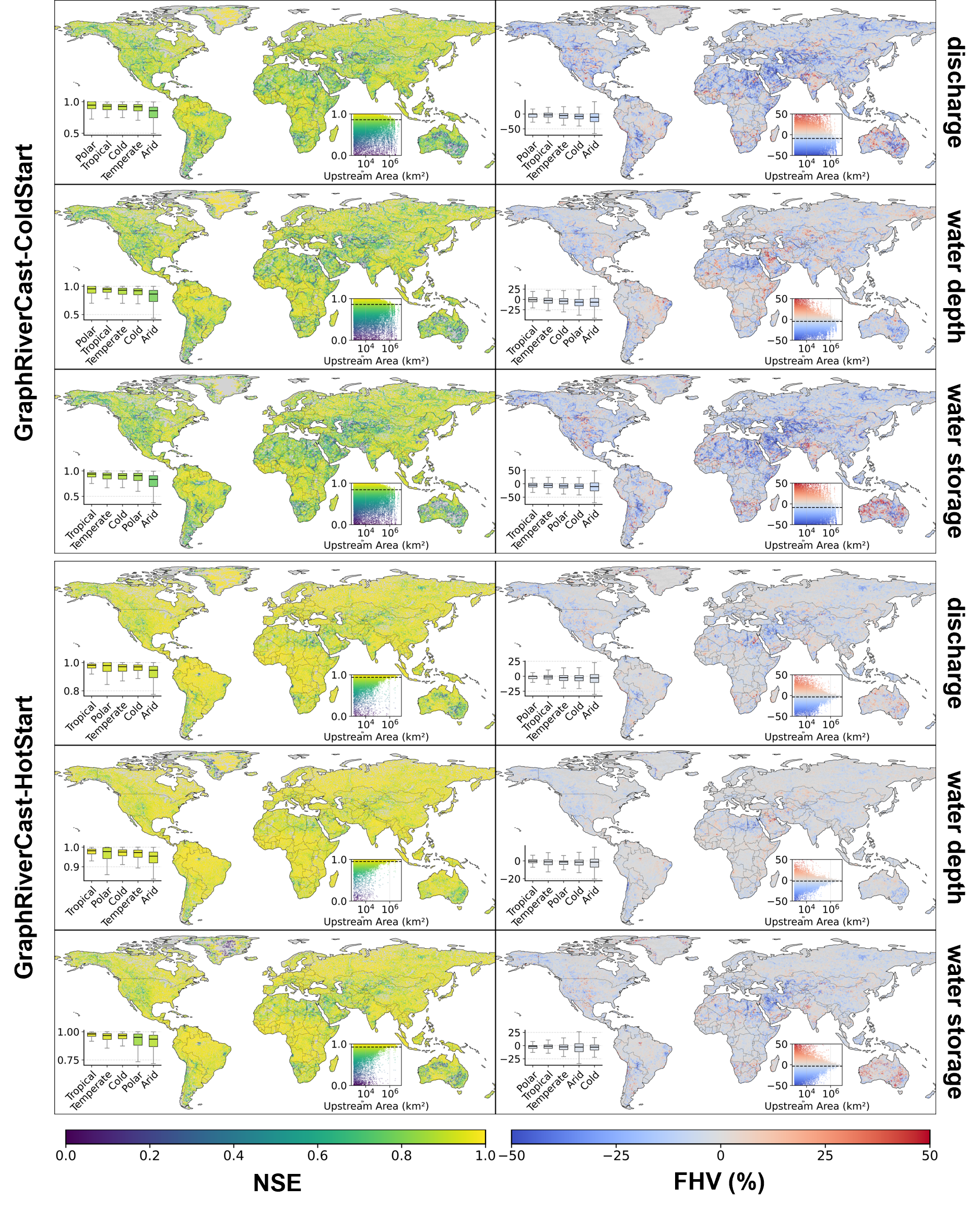
Figure 2 summarizes the global spatial patterns of model performance. Evaluating the GRC-ColdStart mode first reveals the model’s core capability to simulate river hydrodynamics from scratch (Fig. 2, top three rows). In the absolute absence of river state initialization, GRC-ColdStart maintains robust predictive skill following a 20-day spin-up period, which is a necessary phase for synthesizing internal hydrodynamic states from “cold” conditions. Global mean NSE values reached 0.82 for discharge, 0.82 for water depth, and 0.79 for storage, with the highest fidelity observed in tropical and temperate basins. While performance naturally declines in arid zones due to sparse runoff signals and intermittent flow regimes, median skill remains robust for the majority of reaches. Regarding flood-regime biases, high-flow errors remained geographically coherent with global mean FHV values of $-15.4\%$, $-10.5\%$, and $-16.1\%$ for discharge, depth, and storage, respectively. These patterns indicate that the topology-informed AI model effectively infers flow routing and accumulation, reconstructing hydrodynamic propagation solely through graph-based inference. This capability confirms GRC-ColdStart as a viable standalone simulator that does not require initial river states, significantly enhancing global flood forecasting potential in data-sparse regions.

Conversely, the GRC-HotStart mode demonstrates the GRC’s performance ceiling when historical data is accessible (Fig. 2, bottom three rows). When initialized with recent river states, GRC-HotStart achieves high predictive fidelity, yielding global-mean NSE values of approximately 0.93, 0.95, and 0.92 for discharge, water depth, and storage, respectively. Performance remains uniformly robust across climate zones, with the median NSE in tropical and temperate regions exceeding 0.95. Corresponding FHV maps reveal small and spatially stable biases, with global-mean values of $-7.5\%$, $-4.7\%$, and $-7.9\%$ for discharge, depth, and storage, respectively. However, this high accuracy is constrained by a strict input requirement for continuous observational or simulated data. Given that the absence of reliable initial river states is the prevailing norm in global hydrology, this initialization dependency constitutes a significant operational limitation. A SHAP-based feature importance analysis further reveals that the two modes exhibit distinct dependencies on static geomorphic attributes (Extended Data Fig. 1).

Figure 2: Global river hydrodynamic pseudo-hindcasts with GraphRiverCast (GRC). Global spatial distributions of predictive skill relative to CaMa-Flood outputs for river discharge, depth, and storage over the future 7-day horizon, evaluated by the NSE and FHV. Results are presented for GRC-ColdStart (top three rows) and GRC-HotStart (bottom three rows). Boxplots summarize the distribution of performance metrics across major climate zones (Tropical, Temperate, Polar, Cold, and Arid). Inset scatter plots illustrate the relationship between prediction accuracy and river scale based on cumulative upstream area.

Topology boosts ungauged forecasting

While river network topology is a fundamental component of physics-based river models, its necessity in AI-driven hydrology remains a subject of debate^{19, 22, 23, 24}. To resolve this, we systematically evaluated the contributions of three core components within the GRC framework: static features, temporal information, and topological structure, through ablation experiments. By selectively constraining the feature, temporal, and graph modules, we generated a hierarchy of model variants ranging from the full GRC to a baseline Multilayer Perceptron (MLP). These variants span the dominant paradigms of current AI hydrology, enabling an effective assessment of how distinct components and their interactions govern predictive skill²⁹.

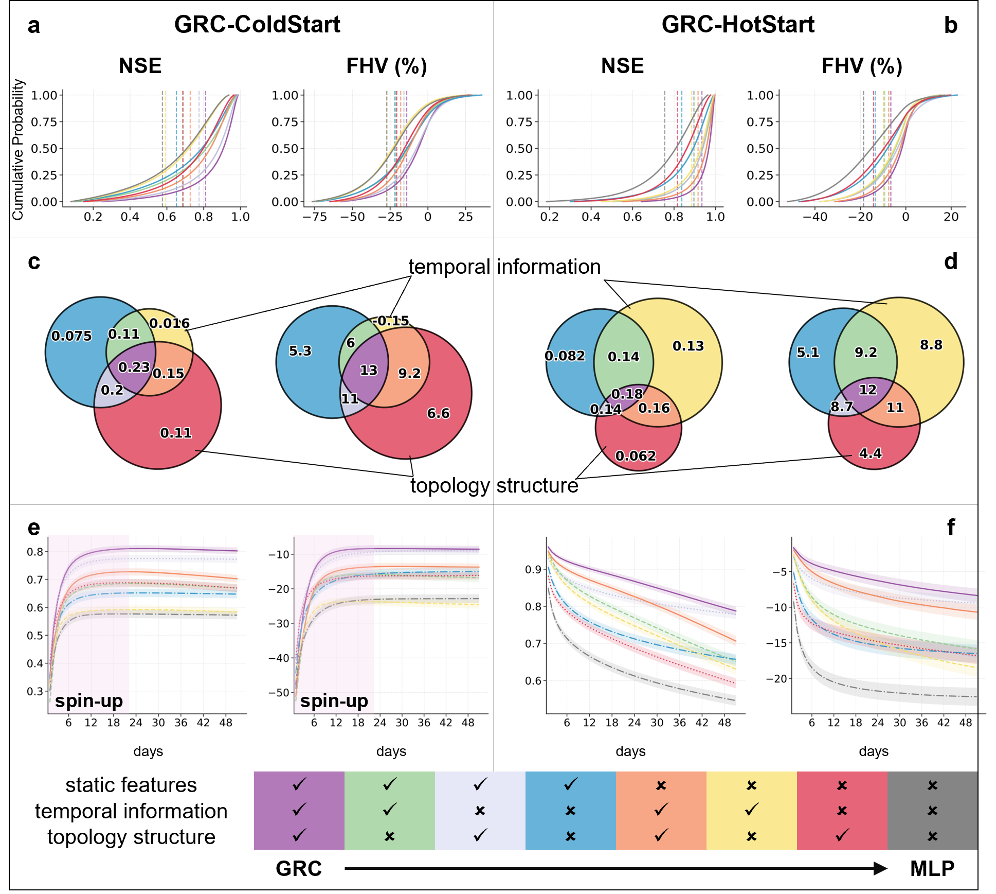
Figures 3a and 3b illustrate the cumulative probability distributions of NSE and FHV for GRC and its simplified variants. Evaluating the GRC-ColdStart mode first (Fig. 3a) reveals the importance of topological structure in the absence of initial conditions. Specifically, excluding topology causes a substantial performance degradation, dropping the mean discharge NSE from 0.82 in the full GRC to 0.69 (Extended Data Table 2). This decline is substantially steeper than the penalty for removing temporal information, which yields an NSE of 0.79. In contrast, the GRC-HotStart mode (Fig. 3b) exhibits a fundamental hierarchy inversion between spatial and temporal dependencies. When initialized with recent states, the full model yields a mean discharge NSE of approximately 0.93 (Extended Data Table 3). However, removing the topological structure in this data-rich setting incurs only a minor penalty, with the NSE dropping to 0.89. This minimal degradation exposes a notable behavioral shift: the presence of historical data substantially reduces the model’s reliance on explicit spatial routing.

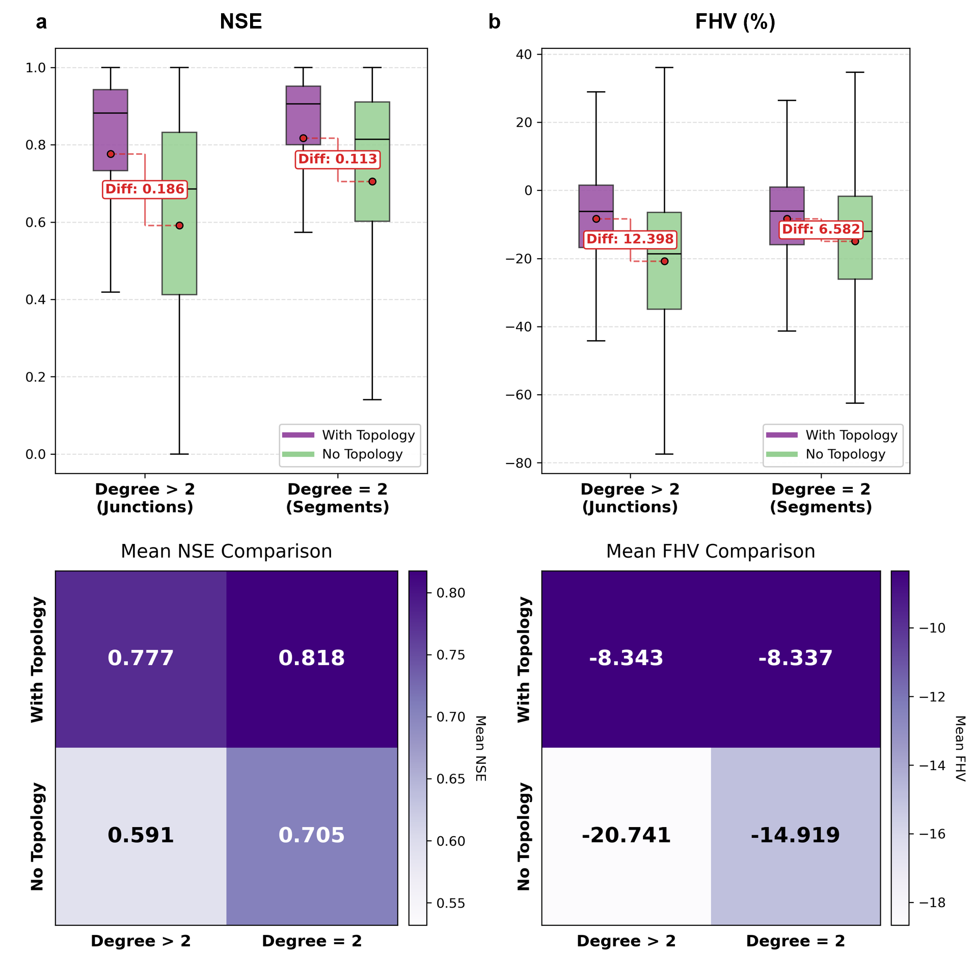
Venn diagrams (Fig. 3c, d) quantify the marginal performance gains attributable to individual components relative to the MLP baseline, further explicitly illustrating this structural shift. In ColdStart mode (Fig. 3c), topology becomes the dominant factor with a unique NSE contribution (0.11) exceeding that of temporal information (0.016) by nearly an order of magnitude. Lacking historical state vectors, the model explicitly depends on topological information to reconstruct the physical coherence of flow propagation. Reach-level analysis further corroborates that topology-informed gains are more pronounced at complex river junctions with higher topological degree (Extended Data Fig. 2). Conversely, in HotStart mode (Fig. 3d), this relationship is reversed. Temporal information dominates with a unique NSE gain of 0.13, which is more than double that of topology (0.062). This reveals an underlying physical redundancy: historical river states inherently encode network topology because they are the direct products of upstream routing. When initialized with these past observations, the model primarily relies on local temporal inertia to predict future states. This historical signal is strong enough to extrapolate short-term trends, bypassing the model’s need to explicitly calculate spatial water exchange across the network. This hidden redundancy explains why previous studies, which evaluated models using historical data, concluded that explicit river topology had limited predictive value.

The temporal evolution of predictive skill reveals distinct trajectories governed by state initialization (Fig. 3e, f). The ColdStart mode (Fig. 3e) follows an asymptotic upward trajectory as the model internally synthesizes hydrodynamic states from forcing data. Here, topology determines the performance ceiling, as the full GRC model achieves the fastest convergence and the highest accuracy plateau. Conversely, in the HotStart mode (Fig. 3f), performance exhibits a characteristic decay across all model variants due to error accumulation typical of autoregressive paradigms. This contrast highlights a critical paradigm shift: in the absence of initial conditions, the model moves beyond statistical extrapolation rooted in temporal inertia to learn intrinsic system dynamics, enabling independent and stable long-term simulations, where explicit topological encoding is essential for reproducing physical routing and accumulation.

Figure 3: Module-wise ablation analysis of GraphRiverCast (GRC). a, b, Cumulative probability distributions of NSE and FHV for the full GRC model and its ablated variants in (a) GRC-ColdStart and (b) GRC-HotStart modes. c, d, Venn diagrams illustrating the specific contributions of each encoding component (static features, temporal information, and topological structure) to predictive skill relative to the MLP baseline. Values represent the marginal NSE and FHV gains for each component and their intersections in (c) ColdStart and (d) HotStart scenarios. e, f, Temporal evolution of performance metrics. e, Evolution of predictive skill in the ColdStart mode, spanning the warm-up period starting from day 1. f, Decay of predictive skill over the forecast horizon in the HotStart mode. Shaded areas indicate the 95% confidence intervals.

Fine-tuning for superior local forecasts

The GRC foundation model is pre-trained on global physics-based simulations, providing a baseline of physical consistency that is nonetheless constrained by inherent model limitations. Conversely, the scarcity of hydrological observations restricts the feasibility of developing fully data-driven models at the global scale. To address this gap, we introduce a pre-training and fine-tuning framework to bridge simulation-trained AI with real-world forecasting. Through fine-tuning, GRC synergizes the generalized physical knowledge encoded in the foundation model with sparse local observational constraints. This strategy effectively leverages both global hydrodynamic patterns and specific in-situ records, overcoming the respective limitations of purely physics-based and data-driven paradigms to achieve superior predictive performance.

This capability was validated through complementary experiments in two representative basins with contrasting characteristics: the vast, minimally regulated Amazon River Basin and the smaller, intensely managed Upper Danube Basin. These experiments were designed to probe the necessity of topological encoding and physics-based pre-training, as well as to verify the model’s cross-scale adaptability. To comprehensively evaluate performance, all fine-tuning experiments were conducted using the GRC-ColdStart mode over continuous multi-year simulation periods. This setup ensures that the model operates as a standalone simulator without reliance on external state initialization, testing its long-term stability. To prevent overfitting and preserve global priors under sparse data conditions, a layer-specific fine-tuning strategy was implemented, where the majority of parameters were frozen while only specific layers were updated (detailed configurations are provided in Methods). Evaluation metrics were computed against real-world in-situ discharge observations rather than simulation outputs. To assess both temporal and spatial generalization, gauging stations were spatially partitioned into a “supervised” subset (used for fine-tuning) and an “unsupervised” subset (completely held out to act as proxies for ungauged reaches). Comparison baselines included the physics-based CaMa-Flood model, the pre-trained foundation model, and a “Scratch” model (randomly initialized and trained solely on local data).

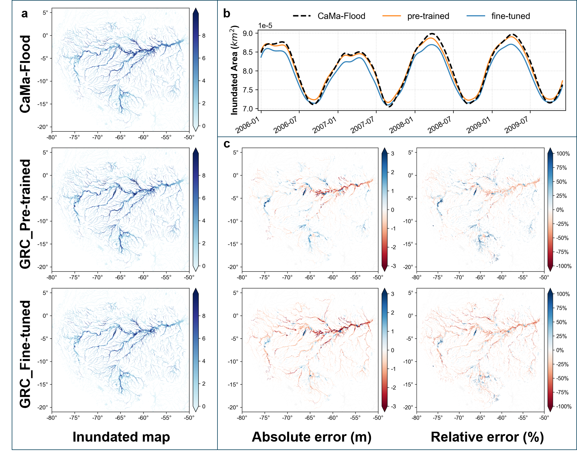
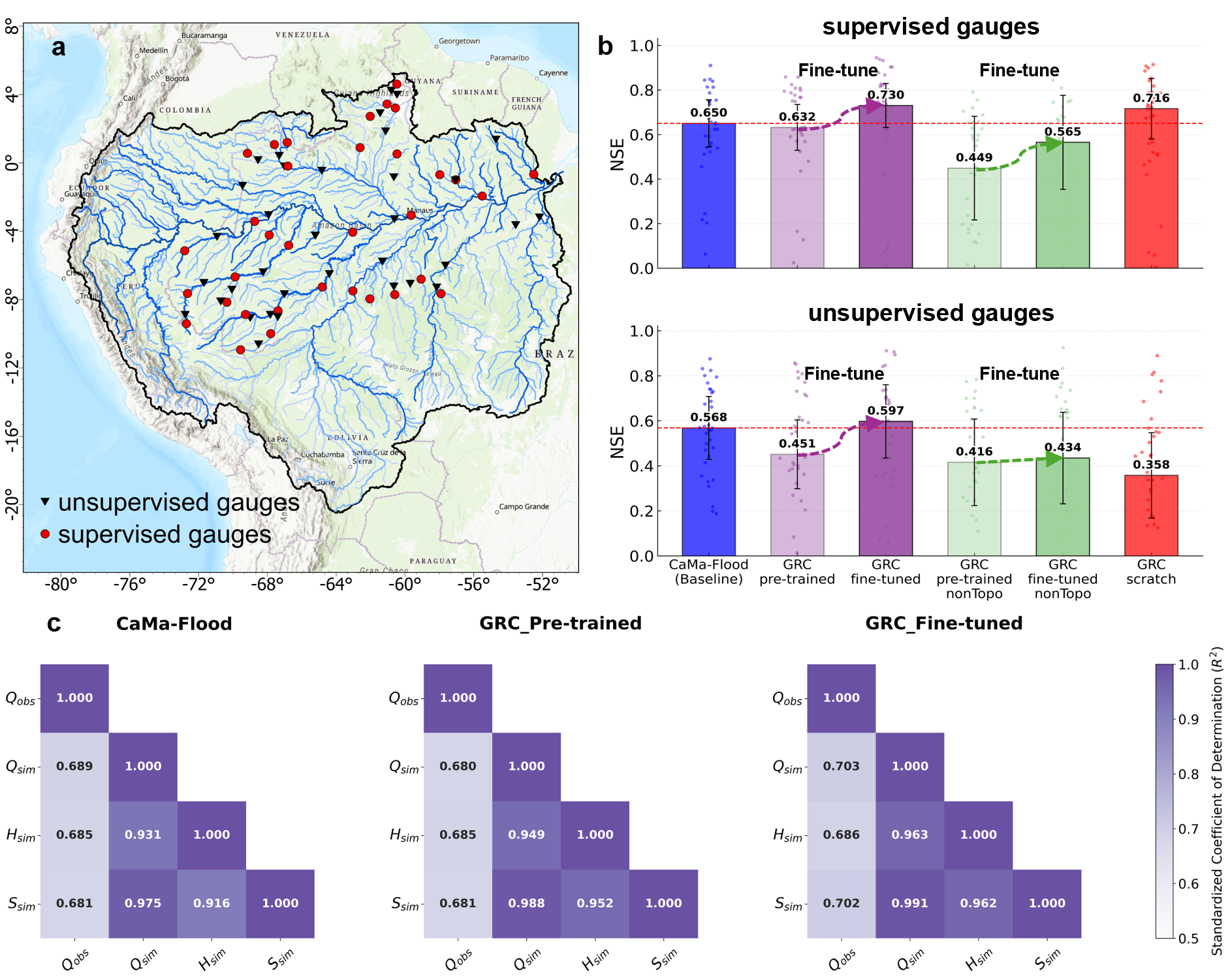
The efficacy of this fine-tuning framework was first evaluated in the Amazon Basin (Fig. 4a). While performance improvements at supervised nodes are expected through fine-tuning, the primary advantage of GRC emerges in its spatial generalization to unmonitored reaches. Following fine-tuning, the predictive accuracy of the GRC model (Fig. 4b, dark purple bars) consistently surpassed the physics-based CaMa-Flood baseline (blue bars), achieving an NSE increase of 0.098 at supervised gauges and a positive gain of 0.146 at unmonitored sites relative to its pre-trained state (light purple bars). Ablation experiments help isolate the mechanisms driving this transfer. The fine-tuned non-topological variant (dark green bars) showed an NSE improvement of 0.116 at supervised gauges relative to its pre-training, yet yielded a negligible gain of merely 0.018 at ungauged sites. This contrast suggests that explicit topological encoding functions as a necessary structural conduit for propagating sparse observational constraints across the network. Furthermore, a purely data-driven model initialized from scratch without pre-training (red bars), representing the conventional paradigm of learning directly from observations, achieved strong performance at supervised stations (NSE = 0.716) but struggled at ungauged reaches, yielding an NSE of merely 0.358. This performance gap, characteristic of spatial overfitting, indicates that physics-based pre-training is important for providing the generalized hydrodynamic priors needed to prevent models from overfitting to local data. Importantly, these accuracy gains were achieved while maintaining multivariate physical consistency. Standardized cross-correlation matrices (Fig. 4c) reveal that as external alignment with observed discharge improved, the internal hydraulic couplings remained highly consistent. This implies that GRC leverages its topological backbone to adjust the broader hydrodynamic regime rather than merely regressing isolated data points, providing spatially continuous boundary conditions suitable for downstream applications like floodplain inundation mapping (Extended Data Fig. 3).

Figure 4: Evaluation of fine-tuning performance and physical consistency against in-situ discharge observations in the Amazon River Basin. a, Spatial distribution of supervised (fine-tuning) and unsupervised (withheld) GRDC stations. b, Predictive skill (NSE) relative to observed discharge for CaMa-Flood, GRC-pre-trained, GRC-fine-tuned, the non-topological variants (GRC-pre-trained_nonTopo, GRC-fine-tuned_nonTopo), and GRC trained from scratch (randomly initialized). These tunable models were trained exclusively on supervised gauges to assess spatial generalization to ungauged reaches. c, Standardized cross-correlation matrices illustrating external alignment with observed discharge ($Q_{\mathrm{obs}}$) and internal physical coupling among simulated states, specifically discharge ($Q_{\mathrm{sim}}$), water depth ($H_{\mathrm{sim}}$), and storage ($S_{\mathrm{sim}}$).

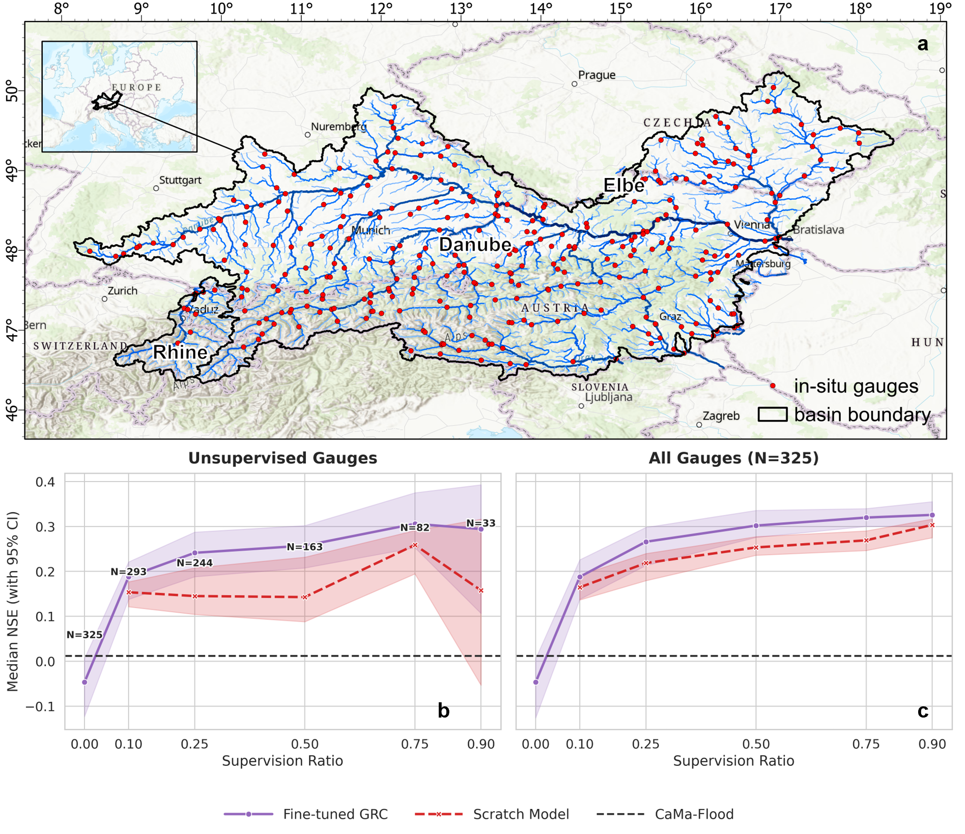
Beyond spatial generalization within a uniform resolution, the cross-scale transferability of the foundation model was subsequently investigated in the Upper Danube Basin. Characterized by dense monitoring networks and intense anthropogenic regulation, this smaller region necessitates a finer spatial resolution to adequately represent its intricate river network. Consequently, this experiment evaluates the direct application of the global foundation model, originally pre-trained exclusively on a coarse spatial grid (15-arc-minute), to a high-resolution regional system (6-arc-minute). Because natural river networks exhibit inherent fractal geometry, their topological structures and the resulting controls on flow routing are fundamentally scale-invariant³⁷. This inherent scale invariance provides the theoretical basis that a coarse global model can effectively inform fine-scale local predictions. As physics-based baselines like CaMa-Flood omit explicit parameterizations for intense human interventions, their simulation accuracy in this highly regulated basin is limited. Inheriting these naturalized flow priors, the zero-shot foundation model also shares this constrained initial fidelity. Under a nested random sampling strategy simulating varying degrees of data scarcity (from 0% to 90% supervision) to assimilate local human management signals, the fine-tuned foundation model consistently outperformed the purely data-driven scratch baseline across all supervision ratios. This performance gap was particularly pronounced at completely unsupervised gauges (Fig. 5b, c). Such an advantage demonstrates that GRC internalizes scale-agnostic topological routing priors rather than merely memorizing grid-specific resolutions. Even without prior exposure to the local high-resolution topology, the foundation model successfully transferred its routing logic, confirming its capacity to exploit the structural self-similarity of river networks for robust fine-scale predictions in ungauged reaches.

Figure 5: Fine-tuning evaluation in the Upper Danube Basin demonstrating cross-scale transferability of the GRC. a, Map of the study domain, showing the river network and the locations of 325 reference gauges (red dots) from the LamaH-CE dataset matched to the 6-arc-minute CaMa-Flood network. b, c, Performance comparison (Median NSE) on unsupervised gauges (b) and all 325 gauges (c) under varying supervision ratios. The plots compare the GRC Foundation Model (purple line), the Scratch Model (red line), and the physical baseline (CaMa-Flood, black dashed line). Annotations (N) in b indicate the number of unsupervised gauges available for evaluation at each ratio. Shaded areas represent the 95% confidence interval.

Discussion

In this study, we present GraphRiverCast (GRC), a topology-informed AI framework that, to the best of our knowledge, represents the first foundation model for global-scale multivariate river simulation. By unifying static geomorphic features, temporal dynamics, and topological structures within a neural-operator architecture, GRC aligns with the non-Euclidean structure of river networks to explicitly capture inter-reach connectivity. This design not only achieves notable improvements in accuracy and predictive stability but also establishes a “pretrain–finetune” paradigm, which marks a transformative advance toward integrating global hydrodynamic knowledge with local observational constraints. Unlike traditional physics-based approaches constrained by high computational costs for model calibration and simulation, GRC supports rapid simulation on standard hardware, offering a scalable solution for global hydrodynamics.

A fundamental theoretical contribution of this work is reconciling prior inconsistencies regarding the utility of river topology in neural hydrological modeling. Comparing the GRC-HotStart and GRC-ColdStart modes reveals that identical architectures rely on fundamentally different information encoding pathways depending on data availability. When historical river states are incorporated, these time series implicitly encode hydrometeorological responses shaped by network connectivity, rendering explicit topological inputs partially redundant. However, global hydrological monitoring is profoundly inequitable, with dense observational networks heavily concentrated in affluent, developed nations, while economically vulnerable regions remain severely under-gauged. This extreme spatial disparity creates a critical hydrological dilemma: the regions most susceptible to climate-driven water disasters are precisely those lacking the historical data requisite for traditional autoregressive forecasting. Consequently, relying on historical state initialization critically bottlenecks real-world deployment and exacerbates global inequalities in disaster preparedness. The GRC-ColdStart mode directly addresses this operational imperative and bridges this observational divide. By inferring flow propagation solely from runoff forcings and static features, the model elevates topology from a redundant input to an indispensable foundational descriptor, ensuring physical coherence and structural consistency across the system. Furthermore, unlike chaotic atmospheric systems, river dynamics are inherently dissipative and asymptotically stable, causing errors from missing initial states to dampen over time³⁰. By capturing these stable, topology-governed dynamics, GRC circumvents excessive reliance on temporal inertia to function as a robust, standalone hydrodynamic simulator capable of long-term operation without error accumulation. This operational independence establishes a highly scalable forecasting foundation for disaster mitigation across the world’s unmonitored and vulnerable regions.

While existing AI-based hydrological models predominantly focus on univariate streamflow prediction, effective water resources management and flood mitigation demand a more comprehensive understanding of river states. The multivariate capability of GRC directly addresses this gap by simultaneously resolving discharge, water depth, and storage across full river networks. This synchronous simulation renders critical hydraulic variables directly available, enabling the model to seamlessly interface with downstream applications such as fluvial flood risk assessment and water resource management. Crucially, this multivariate architecture endows the framework with inherent adaptability to an evolving observational landscape. Global hydrological monitoring systems, encompassing both in-situ networks and satellite remote sensing platforms, are currently undergoing rapid advancement and producing increasingly diverse data types³⁸. A multivariate AI foundation model is uniquely positioned to capitalize on this data explosion. It can seamlessly assimilate these varied emerging observations through the established fine-tuning strategy, driving the continuous evolution of its internalized hydrodynamic representations in tandem with expanding Earth observation networks.

Despite these advances, some limitations and future directions warrant discussion. First, the current GRC foundation model is pre-trained on outputs from a physics-based global river model. Although we aim to learn global hydrodynamic knowledge from state-of-the-art models, existing global river models still face substantial challenges, including forcing uncertainties and limited calibration, which inevitably constrain the quality of the learning priors. Integrating knowledge from multiple physics-based river models may further improve the robustness and generalizability of GRC in the future. Second, regarding anthropogenic interventions, the current foundation model does not explicitly incorporate physical modules for dams and reservoirs. Consequently, simulation fidelity in regions subject to intensive human regulation is inevitably reduced, as the complex operational rules and structural controls are not structurally represented within the model’s physical priors. While fine-tuning with post-construction observational sequences can implicitly capture these regulated flow patterns, achieving true physical fidelity requires explicit structural integration. Incorporating these features remains a formidable challenge at the global scale, primarily due to the scarcity of publicly available operational data and the inherent difficulty in generalizing diverse and often localized water management strategies. Future development will therefore focus on addressing these gaps by integrating specific reservoir operation rules or assimilating water management data to enhance the physical fidelity of simulations in regulated basins.

Moving beyond the model itself, the “pretrain–finetune” paradigm creates the basis for a collaborative global river AI framework. By making the GRC foundation model parameters publicly available, we aim to lower the barriers to high-quality river simulation. This approach allows researchers to leverage a general pre-trained model that can be locally fine-tuned with sparse in-situ data and continually updated as new observations emerge. Subject to data and licensing restrictions, fine-tuned regional models could also be released to the community, fostering knowledge exchange. This paradigm not only advances data-driven hydrology but also provides an adaptive, scalable, and collaborative foundation for sustainable water management worldwide.

Methods and Data

Physics-based global river model

In this research, we adopted the CaMa-Flood global river model as both the baseline and the learning target for the global AI foundation model. CaMa-Flood is one of the most widely used global river hydrodynamic models, simulating river variables—including water storage, discharge, and water surface elevation—from runoff inputs through a river-routing process. The model assumes a one-dimensional linear relationship between river water storage and surface elevation for each river reach and simulates river routing based on the internal continuity and momentum equations originally proposed by Bates et al.³¹.

The runoff forcing used in this study is based on the research of Lin et al. (2019)²⁸, who improved global runoff accuracy through a three-stage bias-reduction pipeline: (i) high-quality multi-source precipitation forcing, (ii) grid-wise bias correction of the runoff distribution using machine-learning–derived percentile targets via sparse CDF matching, and (iii) calibration and evaluation against a large number of discharge gauges. We use this bias-corrected GRADES runoff to drive CaMa-Flood at 15-arc-minute global resolution. From the benchmarking system proposed by Zhou et al. (2025)³², the CaMa-Flood simulations driven by the GRADES runoff outperform both ECMWF and ERA5 runoffs at the global scale and provide a solid baseline for global river modeling, although further regional calibration is still needed for local flood applications.

AI-based global river foundation model (GraphRiverCast)

River Topology and Channel Parameters

The river-network topology and channel parameters used in the GRC model are identical to those in CaMa-Flood, allowing GRC to learn the physics-based routing behavior in an end-to-end manner. The base river topology is derived from the MERIT Hydro global hydrography dataset at ${\sim}$3-arc-second (${\sim}$90 m) resolution²⁶, including flow direction, flow accumulation, elevation, and river centerlines. These fields are upscaled to the 15-arc-minute reach scale using CaMa-Flood’s river-network aggregation and basin delineation procedures (following Yamazaki et al., 2019). Channel attributes are harmonized with the CaMa-Flood parameter set: river slope is derived from MERIT Hydro thalweg gradients; river width is obtained from satellite-based global width datasets (e.g., GRWL and GRWD) or estimated using regionalized width–discharge relationships where observations are sparse; river depth is inferred from empirical hydraulic-geometry relationships tied to width and/or bankfull discharge; and Manning’s $n$ is assigned using land-cover-dependent lookup tables based on literature values. This consistency ensures that the GRC model is exposed to the same network connectivity and hydraulic controls—width, depth, slope, and roughness—that govern flow routing in the physics-based CaMa-Flood framework. Details of the channel parameters are provided in Extended Data Table 1.

GRC Model Structure

GraphRiverCast is formulated as a spatiotemporal deep neural operator designed to capture the complex spatiotemporal dynamics of global river networks. As a neural operator, it establishes a mapping between infinite-dimensional function spaces, providing inherent scalability across temporal and spatial domains. The architecture integrates graph-based non-Euclidean convolution, temporal sequence modeling, and multi-source feature fusion, with full residual connections to facilitate stable training of deep networks³³.

$$\mathcal{O}:(\mathcal{G},\mathcal{S},\mathcal{Y}_{\mathrm{hist}},\mathcal{R})\mapsto\mathcal{Y}_{\mathrm{pred}}$$ (1)

where $\mathcal{O}$ denotes the GraphRiverCast operator; $\mathcal{G}$ represents the river network topology (encoded as a graph); $\mathcal{S}$ is the set of static features; $\mathcal{Y}_{\mathrm{hist}}$ denotes historical river hydrodynamics (for HotStart mode); $\mathcal{R}$ is the sequence of hydrometeorological forcing; and $\mathcal{Y}_{\mathrm{pred}}$ is the predicted future river hydrodynamics over the forecast horizon.

To systematically address the challenge of data scarcity in real-world forecasting, GraphRiverCast (GRC) is designed to operate in two distinct modes: GRC-HotStart and GRC-ColdStart. These modes represent system-level configurations defined by the global availability of historical river state data. In the GRC-HotStart mode, the model assimilates historical river states derived from physics-based simulations (i.e., CaMa-Flood) to emulate data-rich environments where comprehensive initial conditions are available. Conversely, the GRC-ColdStart mode operates independently of historical states, relying solely on static and forcing inputs to simulate completely unmonitored basins. This distinction allows for a comprehensive assessment of model fidelity under varying levels of data observability. The core formulation distinguishing these two operational modes is given by:

$$Y^{(t{:}t+f)}=\begin{cases}\mathrm{GraphRiverCast}\!\left(G,S,Y^{(t-h{:}t-1)},R_{\mathrm{lag}}^{(t-h{:}t-1)},R_{\mathrm{fut}}^{(t{:}t+f)}\right)&\text{, HotStart}\\[6.0pt] \mathrm{GraphRiverCast}\!\left(G,S,R_{\mathrm{lag}}^{(t-h{:}t-1)},R_{\mathrm{fut}}^{(t{:}t+f)}\right)&\text{, ColdStart}\end{cases}$$ (2)

where $Y^{(t{:}t+f)}$ denotes predicted river hydrodynamics (discharge, water depth, storage) over the future time horizon; $G$ represents river network topology (encoding connectivity and directionality); $S$ characterizes static channel geometry (e.g., width, height, elevation); $Y^{(t-h{:}t-1)}$ is historical river hydrodynamics over the historical time horizon; $R_{\mathrm{lag}}^{(t-h{:}t-1)}$ and $R_{\mathrm{fut}}^{(t{:}t+f)}$ denote historical and future hydrometeorological forcing data (runoff), respectively; $h$ is the length of the historical time window; and $f$ is the length of the future forecast window.

Normalization Strategies

To address the scale discrepancy between river reaches (e.g., small tributaries vs. large mainstreams) and ensure fair information fusion, two distinct normalization schemes are applied.

Reach-wise normalization for dynamic variables: Historical and predicted river hydrodynamics (e.g., discharge, water depth) are normalized at the reach level to eliminate magnitude biases:

$$\hat{y}_{i}^{(t)}=\frac{y_{i}^{(t)}-\mu_{y,i}}{\sigma_{y,i}}$$ (3)

where $\mu_{y,i}$ and $\sigma_{y,i}$ are the mean and standard deviation of dynamic variable $y$ at reach $i$ across the training period. This prevents the model from prioritizing large rivers (with higher magnitude dynamics) during convergence.

Global-wise normalization for static features: Static features are normalized globally to ensure consistent scaling during message propagation:

$$\hat{s}_{k}=\frac{s_{k}-\mu_{s,k}}{\sigma_{s,k}}$$ (4)

where $\mu_{s,k}$ and $\sigma_{s,k}$ are the global mean and standard deviation of static feature $s_{k}$ across all reaches. This ensures fair information exchange between reaches with static features at divergent magnitudes in graph convolution.

Information fusion encoders

Static features ($\mathcal{S}$) and dynamic variables (from $\mathcal{Y}_{\mathrm{hist}}$ and $\mathcal{R}$) are first processed through feature enhancement to align their dimensionality and capture cross-feature correlations.

Static feature broadcasting: Static features are temporally broadcasted to match the temporal resolution of dynamic inputs, ensuring each time step retains access to invariant structural information. For a static feature vector $s_{i}$ at reach $i$, broadcasting is defined as:

$$s_{i}^{(t)}=s_{i},\quad\forall\,t\in[1,T]$$ (5)

where $T$ is the number of time steps, and $s_{i}^{(t)}$ denotes the static feature at reach $i$ and time $t$.

Residual feature fusion via MLP: At each time step, input features are formed by concatenating broadcasted static features and dynamic variables. Let $x_{i}^{(t)}$ represent this concatenated input:

$$x_{i}^{(t)}=\mathrm{Concat}\!\left(s_{i}^{(t)},\,y_{i}^{(t-h{:}t-1)},\,r_{i}^{(t-h{:}t-1)}\right)$$ (6)

where $y_{i}^{(t-h{:}t-1)}$ and $r_{i}^{(t-h{:}t-1)}$ are historical river states and hydrometeorological forcing at reach $i$, respectively. Feature fusion is then performed via an MLP with a residual connection, which adds the original input to the MLP output to preserve raw feature information and mitigate gradient degradation in deep networks:

$$f_{i}^{(t)}=x_{i}^{(t)}+\mathrm{MLP}\!\left(x_{i}^{(t)}\right)$$ (7)

To model the directed, non-Euclidean topology of river networks while enhancing feature propagation in deep layers, GRC employs residual Graph Convolutional Network (GCN) units³⁴. This design integrates graph-based spatial convolution with residual connections, which helps preserve raw reach features through deep layers and mitigates the over-smoothing issue common in graph structures. For each reach $i$ in the river network graph $\mathcal{G}$, let $h_{i}^{(l)}\in\mathbb{R}^{d}$ denote the feature vector at the $l$-th GCN layer, where $d$ is the latent space size. The residual GCN layer updates the feature vector by aggregating information from upstream neighbors $\mathcal{N}(i)$ and adding a residual connection:

$$h_{i}^{(l+1)}=h_{i}^{(l)}+\sigma\!\left(\frac{1}{|\mathcal{N}(i)|+1}\Big(W^{(l)}h_{i}^{(l)}+\!\sum_{j\in\mathcal{N}(i)}W^{(l)}h_{j}^{(l)}\Big)+b^{(l)}\right)$$ (8)

where $W^{(l)}\in\mathbb{R}^{d\times d}$ and $b^{(l)}\in\mathbb{R}^{d}$ are learnable parameters; $\sigma(\cdot)$ is a GELU activation function; and the term $\frac{1}{|\mathcal{N}(i)|+1}$ normalizes the aggregated features by the number of neighbors (including the reach itself) to stabilize learning across reaches with varying degrees. When $l=0$, the initial feature vector $h_{i}^{(0)}$ is set to the fused feature $f_{i}$ from the MLP-based feature fusion module.

For the entire river network graph $\mathcal{G}$ with $N$ reaches, the graph convolution operation can be expressed in matrix form. Let $\mathbf{H}^{(l)}\in\mathbb{R}^{N\times d}$ denote the feature matrix at layer $l$, $\mathbf{A}$ the adjacency matrix (with $A_{ij}=1$ if there is an upstream-downstream connection from $j$ to $i$), and $\mathbf{D}$ the degree matrix (a diagonal matrix where $D_{ii}=|\mathcal{N}(i)|+1$):

$$\mathbf{H}^{(l+1)}=\mathbf{H}^{(l)}+\sigma\!\left(\mathbf{D}^{-1}(\mathbf{A}+\mathbf{I})\,\mathbf{H}^{(l)}\,\mathbf{W}^{(l)}+\mathbf{b}^{(l)}\right)$$ (9)

where $\mathbf{I}$ is the identity matrix, ensuring each reach includes its own features in the aggregation, and $\mathbf{D}^{-1}(\mathbf{A}+\mathbf{I})$ represents the normalized adjacency matrix.

The temporal module of GraphRiverCast employs the Gated Recurrent Unit (GRU)³⁵, designed to model the residual term in temporal evolution, specifically capturing the incremental changes relative to the previous time step. For a given time step, let $z^{(t)}$ denote the hidden state encoding temporal information up to $t$, and $h^{(t)}$ represent the spatially fused features (output from residual GCN layers). The GRU module computes a “temporal residual” $\Delta z^{(t)}$. The new hidden state is updated as $z^{(t)}=z^{(t-1)}+\Delta z^{(t)}$, where $\Delta z^{(t)}$ is explicitly modeled by the GRU. The update gate $\Gamma_{u}^{(t)}$ controls how much of the candidate residual is retained, balancing new information with historical trends. The reset gate $\Gamma_{r}^{(t)}$ adjusts the influence of past states, enabling the model to “forget” irrelevant past information. Here $\sigma_{g}(\cdot)$ denotes the sigmoid function:

$$\Gamma_{u}^{(t)} =\sigma_{g}\!\left(W_{u}\cdot\mathrm{Concat}(h^{(t)},z^{(t-1)})+b_{u}\right)$$ (10)

$$\Gamma_{r}^{(t)} =\sigma_{g}\!\left(W_{r}\cdot\mathrm{Concat}(h^{(t)},z^{(t-1)})+b_{r}\right)$$ (11)

$$\widetilde{\Delta z}^{(t)} =\tanh\!\left(W_{z}\cdot\mathrm{Concat}(h^{(t)},\Gamma_{r}^{(t)}\odot z^{(t-1)})+b_{z}\right)$$ (12)

$$\Delta z^{(t)} =\Gamma_{u}^{(t)}\odot\!\left(\widetilde{\Delta z}^{(t)}-z^{(t-1)}\right)$$ (13)

Model and pre-training details

The training pipeline for GRC was implemented using PyTorch Lightning for efficient workflow management and PyTorch Geometric for graph-based operations. The dataset (2010–2019) was temporally partitioned: 2010–2015 for training, 2016–2017 for validation, and 2018–2019 for testing. The river network was represented as a directed graph aligned with the natural flow direction to preserve the physical logic of hydrological propagation.

Regarding network dimensions, feature fusion layers utilized a hidden dimension of 128, while other intermediate processing layers (e.g., temporal and spatial fusion modules) employed 64-dimensional hidden states. To prevent over-smoothing in graph convolution, the GCN component was constrained to 2 layers. The model was trained for 200 epochs with a batch size of 16, employing 16-bit mixed precision to balance computational efficiency and numerical stability. Optimization was performed using the Adam optimizer with an initial learning rate of 0.001. A ReduceLROnPlateau scheduler was applied to decrease the learning rate by a factor of 0.3 if validation loss plateaued (patience = 5 epochs). The loss function utilized a regularized MSELoss to minimize prediction errors while constraining complexity. Early stopping was enforced with a patience of 10 epochs to prevent overfitting.

Layer-specific fine-tuning with sparse data

To efficiently adapt the GRC foundation model to local hydrological regimes while preserving its generalized physical knowledge, a hierarchical fine-tuning protocol characterized by selective parameter freezing and differential optimization was employed. Specifically, the majority of the model’s foundational encoding modules, including the input feature fusion layers, the temporal recurrence unit (GRU), and the shallow graph convolution layers, were frozen to preserve the core spatiotemporal representations learned from global simulations. Optimization was restricted exclusively to the deepest graph convolution layer, which handles high-level spatial refinement, and the final readout layer, which maps latent states to target variables. To further mitigate the risk of catastrophic forgetting and ensure stable convergence, distinct learning rates were assigned to these unfrozen components based on their network depth. The final readout layer was updated with a baseline fine-tuning rate (set to $1\times 10^{-5}$), whereas the unfrozen deep graph convolution layer was updated at a strictly reduced magnitude (10% of the baseline rate). This conservative adjustment strategy ensures that the model’s internal routing logic is only minimally perturbed, allowing the topological propagation mechanism to remain robust while precisely calibrating the output mapping to match local observational distributions.

This fine-tuning paradigm was validated in the Amazon River Basin, utilizing historical discharge records from the GRDC as ground truth. To ensure high data quality and temporal consistency, stations were rigorously screened based on three criteria: geospatial location within the Amazon Basin boundaries, continuous temporal coverage spanning the full study period from January 1, 2000, to December 31, 2009, and high data integrity, where only stations with a missing data ratio of $<$10% were retained. This screening process yielded 68 high-quality stations. To evaluate the model’s spatiotemporal generalization capabilities, the dataset was partitioned along both temporal and spatial dimensions. Temporally, data from 2000–2005 served as the training set for fine-tuning, while the period from 2006–2007 was used for validation, and 2008–2009 was strictly reserved for independent out-of-time testing. Spatially, stations were randomly partitioned across the topological network into a supervised set (50%) used for fine-tuning and an unsupervised set (50%) withheld completely from training to assess performance in ungauged reaches. Notably, the supervised stations represent less than 1% of the total river reaches in the Amazon network, imposing a stringent test on the model’s ability to propagate information via topological connectivity.

Cross-scale fractal transferability experiment

We aligned observational records from the LamaH-CE dataset with the model’s 6-arc-minute river topology (derived from CaMa-Flood). To ensure physical consistency, reference gauges were identified using a two-step spatial filter: (1) a search radius of 0.1415° (${\sim}$15 km), and (2) a strict contributing area error threshold of $<$10%. This process yielded 325 high-quality gauges (Fig. 5a).

To evaluate performance across varying data regimes, we implemented a nested sampling strategy. The 325 gauges were randomly shuffled (fixed seed) and sliced into cumulative subsets of 10%, 25%, 50%, 75%, 90%, and 100%. This nested design ensures that smaller subsets are strictly contained within larger ones, thereby isolating the effect of observation density from site-specific variability.

We operated the models in ColdStart mode to assess state synthesis capabilities. Fine-tuning was conducted using data from 2000–2009, followed by evaluation on an independent validation period (2010–2017). For the foundation model configurations, we employed the same parameter freezing strategy as in the Amazon Basin experiment: only the readout and deep graph layers were updated, while the foundational spatiotemporal encoders remained frozen. In contrast, all parameters were subject to optimization for the Scratch Model.

Evaluation metrics

Two metrics were employed to evaluate the performance of GRC in simulating river hydrodynamics, capturing both the overall predictive skill and extreme flow behavior. Where $\hat{Y}$ denotes the predicted value and $Y$ denotes the corresponding true value, the metrics are defined as follows:

Nash–Sutcliffe Efficiency (NSE) quantifies overall agreement between simulated and true values across the entire forecast window:

$$\mathrm{NSE}=1-\frac{\sum_{f=1}^{F}(\hat{Y}^{(t+f)}-Y^{(t+f)})^{2}}{\sum_{f=1}^{F}(Y^{(t+f)}-\bar{Y})^{2}}$$ (14)

where $F$ is the total length of the future forecast window and $\bar{Y}$ is the mean of true values over all $F$ time steps. NSE ranges from $-\infty$ to 1, with 1 indicating perfect agreement.

High-Flow Volume Bias (FHV) measures bias in simulating top 2% flows (exceedance probability $<$ 0.02) within the window:

$$\mathrm{FHV}=\frac{\sum_{h=1}^{H}(\hat{Y}_{h}-Y_{h})}{\sum_{h=1}^{H}Y_{h}}\times 100$$ (15)

where $H$ is the number of high-flow samples (top 2% of all values), and $\hat{Y}_{h}$ and $Y_{h}$ are the simulated and true values for the $h$-th high-flow sample.

To elucidate the influence of static geomorphic attributes on model predictions and verify the physical rationality of the learned representations, we employed SHAP (SHapley Additive exPlanations)³⁶. Originating from cooperative game theory, the SHAP framework assigns an importance value to each input feature, representing its marginal contribution to the model’s output relative to a baseline. In this study, the mean absolute SHAP value was calculated for each static feature across the test dataset to derive a global importance ranking. This quantification enables a comparative analysis of feature dependencies between the GRC-HotStart and GRC-ColdStart modes, revealing how data availability shifts the model’s reliance on specific physical descriptors.

Extended Data

Extended Data Table 1 $\mid$ Data structure of GraphRiverCast.

Category	Variable	Description	Unit	Format
Forcing	runoff	Runoff generated by the watershed	m3/s	N$\times$t
Hydrodynamics	discharge	River discharge	m3/s	N$\times$t
	water depth	Water depth in the river channel	m	N$\times$t
	storage	Water storage in river-controlled area	m3	N$\times$t
Static features	ctarea	Catchment area	m2	N$\times$1
	elevtn	Elevation at channel outlet	m	N$\times$1
	grdarea	Gridded area of watershed	m2	N$\times$1
	nxtdst	Distance to next river basin	m	N$\times$1
	rivlen	Length of river channel	m	N$\times$1
	rivwth_gwdlr	River width (GWDLR dataset)	m	N$\times$1
	uparea	Upstream catchment area	m2	N$\times$1
	width	Channel width at outlet	m	N$\times$1
	fldhgt	Floodplain elevation parameters	m	N$\times$10
Topology	Graph	River network connectivity	–	M$\times$M

Extended Data Table 2 $\mid$ Ablation experiment metrics for GRC-ColdStart.

Ablated variant			Discharge		Water depth		Water storage
Stat	Temp	Topo	NSE	FHV(%)	NSE	FHV(%)	NSE	FHV(%)
$\checkmark$	$\checkmark$	$\checkmark$	0.82	–15.4	0.82	–10.5	0.79	–16.1
$\checkmark$	$\checkmark$	$\times$	0.69	–24.6	0.71	–14.9	0.66	–23.8
$\checkmark$	$\times$	$\checkmark$	0.79	–17.5	0.79	–12.2	0.75	–17.9
$\checkmark$	$\times$	$\times$	0.66	–25.1	0.67	–16.2	0.63	–24.2
$\times$	$\checkmark$	$\checkmark$	0.74	–19.6	0.75	–13.7	0.70	–20.5
$\times$	$\checkmark$	$\times$	0.59	–31.5	0.63	–19.9	0.56	–30.4
$\times$	$\times$	$\checkmark$	0.70	–22.8	0.71	–15.7	0.66	–23.1
$\times$	$\times$	$\times$	0.58	–31.3	0.60	–19.9	0.55	–30.2

Extended Data Table 3 $\mid$ Ablation experiment metrics for GRC-HotStart.

Ablated variant			Discharge		Water depth		Water storage
Stat	Temp	Topo	NSE	FHV(%)	NSE	FHV(%)	NSE	FHV(%)
$\checkmark$	$\checkmark$	$\checkmark$	0.93	–7.5	0.95	–4.7	0.92	–7.9
$\checkmark$	$\checkmark$	$\times$	0.89	–10.9	0.92	–6.6	0.88	–10.8
$\checkmark$	$\times$	$\checkmark$	0.89	–10.6	0.91	–7.8	0.88	–11.3
$\checkmark$	$\times$	$\times$	0.83	–15.0	0.86	–10.3	0.82	–15.2
$\times$	$\checkmark$	$\checkmark$	0.91	–8.4	0.94	–5.7	0.90	–8.8
$\times$	$\checkmark$	$\times$	0.87	–11.2	0.91	–7.1	0.87	–11.1
$\times$	$\times$	$\checkmark$	0.80	–15.5	0.85	–10.2	0.80	–17.1
$\times$	$\times$	$\times$	0.74	–20.5	0.80	–12.7	0.73	–22.7

Extended Data Fig. 1 $\mid$ SHAP-based feature importance analysis of static variables. a, b, SHAP summary plots illustrating the contribution of static geomorphic features to model predictions of discharge, water depth, and storage (left to right) in (a) GRC-ColdStart and (b) GRC-HotStart modes. Features are ordered vertically by their mean absolute SHAP values, which quantify their impact on the model output. The plots demonstrate that the ranking of feature importance varies distinctively between the two modes and across output variables, with different static variables emerging as the primary contributors in each configuration.

Extended Data Fig. 2 $\mid$ Topology-informed performance gains across river reaches of varying topological complexity. a, b, Comparative analysis of predictive skill (NSE and FHV) for the GRC-ColdStart mode at high-degree nodes (degree $>$2, corresponding to complex confluences and bifurcations) versus linear river segments (degree $=$2). Boxplots summarize the performance distributions for the topology-informed GRC relative to non-topological baselines. The comparison reveals a positive correlation between reach-level topological complexity and predictive gain: the explicit encoding of topology yields significantly larger accuracy improvements at high-degree junctions compared to simple linear segments. This trend confirms that topological information is particularly critical for resolving complex flow mixing and redistribution dynamics at river intersections.

Extended Data Fig. 3 $\mid$ Comparison of fluvial flood inundation in the Amazon Basin. a, Spatial distribution of maximum inundation depths calculated over the 2006–2010 period. Maps display flood extents generated by coupling output water depths from CaMa-Flood, GRC-pre-trained, and GRC-fine-tuned simulations with the MERIT DEM. b, Time series of total inundation extent. The temporal comparison reveals that while the pre-trained model closely follows the baseline, the GRC-fine-tuned results exhibit a reduced total inundation area, indicating a tendency to mitigate the systemic overestimation of flood risk often associated with the physics-based CaMa-Flood model. c, Quantitative error analysis relative to the CaMa-Flood baseline. Plots display the absolute error and relative error of simulated water depths for the GRC model at both pre-training and fine-tuning stages.

References

- 1 ECA, U. et al. Water and Climate Change. (UNESCO, 2020).
- 2 Ebi, K. L. et al. Extreme Weather and Climate Change: Population Health and Health System Implications. Annu. Rev. Public Health 42, 293–315 (2021).
- 3 Lee, J., Perera, D., Glickman, T. & Taing, L. Water-related disasters and their health impacts: A global review. Prog. Disaster Sci. 8, 100123 (2020).
- 4 Delforge, D. et al. The EM-DAT Emergency Events Database Archive. Open Data @ UCLouvain https://doi.org/10.14428/DVN/I0LTPH (2025).
- 5 World Meteorological Organization. Early Warnings for All: Factsheet. (2024).
- 6 Yamazaki, D. The global hydrodynamic model CaMa-Flood (version 3.6.2). JAMSTEC (2014).
- 7 Mizukami, N. et al. mizuRoute version 1: a river network routing tool for a continental domain water resources applications. Geosci. Model Dev. 9, 2223–2238 (2016).
- 8 Xu, Q. et al. Physics-aware Machine Learning Revolutionizes Scientific Paradigm for Machine Learning and Process-based Hydrology. Preprint at https://doi.org/10.48550/arXiv.2310.05227 (2024).
- 9 Lam, R. et al. GraphCast: Learning skillful medium-range global weather forecasting. Preprint at https://doi.org/10.48550/arXiv.2212.12794 (2023).
- 10 Bi, K. et al. Accurate medium-range global weather forecasting with 3D neural networks. Nature 619, 533–538 (2023).
- 11 Ho, L. & Goethals, P. Machine learning applications in river research: Trends, opportunities and challenges. Methods Ecol. Evol. 13, 2603–2621 (2022).
- 12 Langhorst, T., Andreadis, K. M. & Allen, G. H. Global cloud biases in optical satellite remote sensing of rivers. Geophys. Res. Lett. 51, e2024GL110085 (2024).
- 13 Alkama, R., Marchand, L., Ribes, A. & Decharme, B. Detection of global runoff changes: results from observations and CMIP5 experiments. Hydrol. Earth Syst. Sci. 17, 2967–2979 (2013).
- 14 World Meteorological Organization. State of Global Water Resources 2022. (2023).
- 15 Nearing, G. et al. Global prediction of extreme floods in ungauged watersheds. Nature 627, 559–563 (2024).
- 16 Eddin, M. H. S., Zhang, Y., Kollet, S. & Gall, J. RiverMamba: A State Space Model for Global River Discharge and Flood Forecasting. Preprint at https://doi.org/10.48550/arXiv.2505.22535 (2025).
- 17 Lorenz, E. N. Deterministic nonperiodic flow. in Universality in Chaos (2nd edn) 367–378 (Routledge, 2017).
- 18 Yang, C. T., Song, C. C. S. & Woldenberg, M. J. Hydraulic geometry and minimum rate of energy dissipation. Water Resour. Res. 17, 1014–1018 (1981).
- 19 Zhao, S. et al. Beyond Grid Data: Exploring graph neural networks for Earth observation. IEEE Geosci. Remote Sens. Mag. 13, 175–208 (2025).
- 20 Sun, A. Y., Jiang, P., Yang, Z.-L., Xie, Y. & Chen, X. A graph neural network (GNN) approach to basin-scale river network learning: the role of physics-based connectivity and data fusion. Hydrol. Earth Syst. Sci. 26, 5163–5184 (2022).
- 21 Deng, L., Zhang, X., Slater, L. J., Liu, H. & Tao, S. Integrating Euclidean and non-Euclidean spatial information for deep learning-based spatiotemporal hydrological simulation. J. Hydrol. 638, 131438 (2024).
- 22 Zhang, Z., Tian, W., Lu, C., Liao, Z. & Yuan, Z. Graph neural network-based surrogate modelling for real-time hydraulic prediction of urban drainage networks. Water Res. 263, 122142 (2024).
- 23 Kirschstein, N. & Sun, Y. The Merit of River Network Topology for Neural Flood Forecasting. Preprint at http://arxiv.org/abs/2405.19836 (2024).
- 24 Wang, H., Chen, J., Zheng, Y. & Song, X. Accelerating flood warnings by 10 hours: the power of river network topology in AI-enhanced flood forecasting. npj Nat. Hazards 2, (2025).
- 25 Lehner, B., Verdin, K. & Jarvis, A. New Global Hydrography Derived From Spaceborne Elevation Data. EoS Trans. 89, 93–94 (2008).
- 26 Yamazaki, D. et al. MERIT Hydro: A High-Resolution Global Hydrography Map Based on Latest Topography Dataset. Water Resour. Res. 55, 5053–5073 (2019).
- 27 Wortmann, M. et al. Global River Topology (GRIT): A Bifurcating River Hydrography. Water Resour. Res. 61, e2024WR038308 (2025).
- 28 Lin, P. et al. Global Reconstruction of Naturalized River Flows at 2.94 Million Reaches. Water Resour. Res. 55, 6499–6516 (2019).
- 29 Ng, K. W. et al. A review of hybrid deep learning applications for streamflow forecasting. J. Hydrol. 625, 130141 (2023).
- 30 Bastin, G. et al. On Lyapunov stability of linearised Saint-Venant equations for a sloping channel. Networks Heterogen. Media 4, 177–187 (2009).
- 31 Bates, P. D., Horritt, M. S. & Fewtrell, T. J. A simple inertial formulation of the shallow water equations for efficient two-dimensional flood inundation modelling. J. Hydrol. 387, 33–45 (2010).
- 32 Zhou, X., Yamazaki, D., Revel, M., Zhao, G. & Modi, P. Benchmark Framework for Global River Models. J. Adv. Model. Earth Syst. 17, e2024MS004379 (2025).
- 33 He, K., Zhang, X., Ren, S. & Sun, J. Deep Residual Learning for Image Recognition. in Proc. CVPR (2016).
- 34 Kipf, T. N. & Welling, M. Semi-Supervised Classification with Graph Convolutional Networks. in Proc. ICLR (2017).
- 35 Cho, K. et al. Learning Phrase Representations using RNN Encoder–Decoder for Statistical Machine Translation. in Proc. EMNLP 1724–1734 (2014).
- 36 Lundberg, S. M. & Lee, S.-I. A unified approach to interpreting model predictions. Adv. Neural Inf. Process. Syst. 30 (2017).
- 37 Rodriguez-Iturbe, I. & Rinaldo, A. Fractal River Basins: Chance and Self-Organization. (Cambridge Univ. Press, 1997).
- 38 Andreadis, K. M. et al. A First Look at River Discharge Estimation From SWOT Satellite Observations. Geophys. Res. Lett. 52, e2024GL114185 (2025).