Support Tokens, Stability Margins, and a New Foundation for Robust LLMs

Abstract

Self-attention is usually described as a flexible, content-adaptive way to mix a token with information from its past. We re-inpterpret causal self-attention transformers that are the backbone of modern day foundation models in a probabilistic framework much like classical PCA are interpreted as probabilistic PCA. But there is a further twist - surprisingly, due to a change in variable pheonomenon, a barrier constraint emerges on the self attention parameters that induces a fascinating geometry on the token space which provides interesting insights on how decoding works in LLMs. It shows there is a boundary where attention becomes ill-conditioned and this leads to a margin interpretation, similar to classical support vector machines. Just like support vectors, this naturally gives rise to the concept of support tokens.

Furthermore, we show that LLMs can be interpreted as stochastic process over the power set of token space providing a rigorous probabilistic framework for modeling. We propose a Bayesian framework and provide a MAP estimation recipe that works with a very simple modification of how LLMs are trained today - all we need is an additional penalty term that is a smooth log-barrier in addition to the LLM cross-entropy objectives. We show this provides more robust models without sacrificing out of sample accuracy and is easy to incorporate in practice.

Keywords Large Language Models $\cdot$ Robustness $\cdot$ Causal Attention $\cdot$ Large Margins $\cdot$ Stochastic Processes $\cdot$ Bayesian prior $\cdot$ MAP $\cdot$ Jacobian $\cdot$ Probabilistic Models

1 Introduction

Transformers are the default architecture for sequence modeling across language, vision, and beyond (Vaswani et al., 2017; Brown et al., 2020; Dosovitskiy et al., 2021). The heart of transformers is causal self-attention that is often described as a content-adaptive weighted average: each token mixes information from its past according to similarity scores. Moving beyond this colloquial description, we ask a formal question:

Does causal self-attention admit an explicit probabilistic interpretation, and if so, what does that interpretation imply about the geometry and inductive bias of the model?

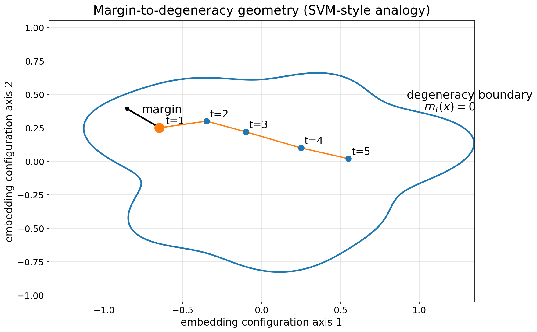
In this paper, we give a concrete answer. We show that causal self-attention is interpreted as a probabilistic model on embeddings (treated as latent variables). But the most striking result is a barrier constraint on the parameters of self-attention that emerges through this probabilistic formulation; and this induces a nice geometry that leads to interesting ramifications. It shows that there is a boundary in the latent space where the attention-induced mapping becomes locally ill-conditioned. This defines a margin to degeneracy—a novel quantitative measure we introduce of how far each position is from that unstable boundary. This in turn helps us understand which tokens matter the most (Figure 1.1). This in turn helps us understand which tokens matter the most. The stability of a sequence is governed by its margin across positions. Tokens whose contexts are closest to degeneracy become the bottlenecks that dominate the barrier signal, directly analogous to support vectors in large-margin classifiers (Cortes and Vapnik, 1995).

Figure 1.1: Margin-to-degeneracy geometry (SVM-style analogy). The curve denotes an instability boundary: configurations where the attention-induced latent-noise map becomes locally ill-conditioned (small perturbations can lead to ambiguous or disproportionate changes). A sequence traces a trajectory of embedding configurations across token positions (dots). The margin of a token is its distance to this boundary (arrow). In this schematic, token 1 is the support token because it has the smallest margin (it lies closest to instability), so it governs the sequence-level stability margin and dominates the barrier pressure. This mirrors SVMs, where support vectors are the points closest to the decision boundary and therefore determine the margin. (Precise definitions appear in Section 3.)

The story does not end here. During decoding, when within the boundary, sign of a functional creates both an attractive and repulsive coupling kind of behavior on attentions - for positive value of this function, it encourages the attention to cluster around similar tokens, and for negative it spreads the attention across highly dispersed tokens. This sign-dependent attractive/repulsive behavior is reminiscent of classical spin-coupling phenomena in the Ising model (Ising, 1925).

The “support token” perspective provides an interpretable explanation for where the additional likelihood pressure concentrates and motivates a practical training lever: adding (or stably approximating) the barrier term yields a controllable tradeoff between data fit and geometric conditioning of attention, analogous to classical regularization paths in regression models (Tibshirani, 1996; Efron et al., 2004).

Practically, the probabilistic formulation yields an immediate optimization lens. We work in a Bayesian framework (Bishop, 2006; Murphy, 2012) where the usual transformer model of tokens conditioned on embeddings is treated as log-likelihood and we compose it with a log-prior based on a probabilistic causal transformer we identify in this paper. Writing down the log-posterior and estimating MAP produces the familiar data-fit term together with a barrier term that enforces stability. This connects causal self-attention to classical constrained estimation (Boyd and Vandenberghe, 2004): maximizing posterior is equivalent to optimizing a squared-error objective (at noise scale $\sigma$) under implicit margin constraints that keep the attention mapping well-behaved.

Beyond the single-layer self-attention mechanism, we also clarify how depth composes. In particular, we show how deep transformers can be interpreted as a hierarchical probability model across layers and we show that the usual large language models are a stochastic process over the power set of all tokens.

Contributions.

1. A probabilistic interpretation of causal self-attention. We formalize a causal self-attention layer as a conditional probability model over latent embeddings, which in turn induces a joint probability law over token sequences with an exact likelihood.

2. Margin to degeneracy and a stability-inducing log-barrier. We show that the induced likelihood contains an additional term that defines a margin to a critical degeneracy boundary and yields a smooth barrier against locally unstable attention geometries (Theorem 1).

3. Optimization view. We show that the log-likelihood can be written as a squared-error objective at noise scale $\sigma$ together with a margin-based barrier term. Thus, our framework reinterprets existing transformers probabilistically rather than replacing them with a different model.

4. A model-implied training penalty and empirical evidence. Using a Bayesian formulation and MAP estimation (Bishop, 2006; Murphy, 2012), we derive a training penalty induced directly by the probabilistic model. This penalty requires no architectural modification and can be added to standard LLM training objectives; in our experiments, it improves robustness of the trained model.

5. Depth as a hierarchy of conditional priors. We characterize how the probabilistic interpretation composes across depth and identify conditions under which the nontrivial volume correction localizes to the first layer under standard transformer conditioning. This explains why a one-layer probabilistic causal prior is already a natural practical choice in the Bayesian setting.

Organization

Section 2 introduces our latent-noise view of causal self-attention as a structural (graphical) model over embeddings. Section 3 develops the single-layer theory, derives the margin/log-barrier term induced by token-dependent attention, and connects the probabilistic objective to the familiar deterministic transformer via the $\sigma\to 0$ limit, yielding a practical penalty formulation. Section 4 revisits these results from an optimization perspective and clarifies the resulting training objective and constraints. Section 5 establishes that the induced family of token distributions is consistent across sequence lengths (i.e., defines a well-posed stochastic process), which is the key technical ingredient for learning from datasets of variable-length sequences. Section 6 extends the interpretation to depth, showing how layers compose into a hierarchy of conditional priors and how the correction terms behave under standard conditioning. Section 7 evaluates the resulting penalty empirically. All proofs are deferred to the Appendix.

2 A Latent-Noise View of Causal Self-Attention

This section introduces the probabilistic object for causal self-attention that is the core of the paper. The goal is not to modify the transformer architecture, but to make explicit the distribution over the model’s embeddings (hidden states) that a causal self-attention layer implicitly defines when viewed as a generative mechanism.

Fix a sequence length $L$ and an embedding dimension $d$. We write

$$x_{1:L}=(x_{1},\dots,x_{L}),\qquad x_{t}\in\mathbb{R}^{d},$$

for the sequence of continuous embeddings (hidden states) produced by a transformer (Vaswani et al., 2017; Brown et al., 2020). When we need to refer to depth, we write $x_{t}^{(\ell)}$ for the layer-$\ell$ embedding, with $x_{t}^{(0)}$ the input token embedding. We assume, without loss of generality for this discussion that the embeddings are detrended because we can also work with the residuals. For most of the paper, depth suffix won’t be needed to understand the core concepts and it is fine to ignore that during first reading.

The transformer ultimately is used to define a probability model over discrete tokens via cross-entropy loss, but its computation proceeds through these continuous embeddings. Our focus in this paper is: what probabilistic structure does causal self-attention induce over the embedding sequence $x_{1:L}$?

We make a simple modeling move: we treat embeddings as random variables rather than fixed activations. Concretely, we posit that embeddings are generated sequentially from latent noise,

$$\varepsilon_{1:L}=(\varepsilon_{1},\dots,\varepsilon_{L}),\qquad\varepsilon_{t}\in\mathbb{R}^{d},$$

through a causal transformation. This is the same conceptual step that turns deterministic estimators into probabilistic models (e.g., probabilistic PCA (Tipping and Bishop, 1999), see also standard latent-variable modeling treatments (Bishop, 2006; Murphy, 2012)).

Throughout the main text we will use an isotropic Gaussian base noise,

$$\varepsilon_{t}\sim\mathcal{N}(0,\sigma^{2}I_{d}),$$ (1)

where $\sigma>0$ controls the noise scale (and later enables a clean “zero-noise” limit back to the usual deterministic view).

2.1 Causal self-attention as a probabilistic model over embeddings

Consider a single self-attention layer. For clarity, we start with a single head and write the usual query/key/value projections

$$q_{t}=W_{Q}x_{t},\qquad k_{s}=W_{K}x_{s},\qquad v_{s}=W_{V}x_{s}.$$

Causal self-attention forms a context summary $\mu_{t}$ by attending to the past. In the strict causal form, (Vaswani et al., 2017; Brown et al., 2020)

$$\alpha_{ts}(x)\;=\;\frac{\exp\!\left(q_{t}^{\top}k_{s}\right)}{\sum_{r<t}\exp\!\left(q_{t}^{\top}k_{r}\right)},\qquad s<t,\qquad\mu_{t}(x)\;=\;\sum_{s<t}\alpha_{ts}(x)\,v_{s}.$$ (2)

The standard deterministic view treats $\mu_{t}$ as an update computed from the current embedding. Our probabilistic view instead treats $\mu_{t}$ as the mean of a probability model for $x_{t}$ given its context, with additive latent noise:

$$x_{t}\;=\;\mu_{t}(x)\;+\;\varepsilon_{t},\qquad\varepsilon_{t}\sim\mathcal{N}(0,\sigma^{2}I_{d}).$$ (3)

The key modeling point is that $\mu_{t}(x)$ is both causal (it uses only earlier positions) and token-dependent: the weights $\alpha_{ts}(x)$ depend on the current token through the query $q_{t}=W_{Q}x_{t}$.

It is convenient to write (3) in residual form:

$$\varepsilon_{t}\;=\;e_{t}(x)\;\triangleq\;x_{t}-\mu_{t}(x).$$ (4)

This defines a transformation between latent variables $\varepsilon_{1:L}$ and embeddings $x_{1:L}$, and it is this transformation that we analyze throughout the paper.

Remark   Standard “causal” transformer implementations often include the current position in the context (i.e., they allow $s\leq t$) (Radford et al., 2019; Brown et al., 2020), which introduces a nonzero self-weight $\alpha_{tt}$ and a self-value term $v_{t}$ inside $\mu_{t}$. Our main results and interpretations do not hinge on excluding $s=t$: the same token-dependent mechanism remains, and the induced likelihood still acquires an additional stability/conditioning term. We present the strict-causal setup (2) in the main text because it yields the cleanest exposition (and a directly autoregressive interpretation). The modifications for $s\leq t$ are straightforward and are stated in Appendix A.

2.2 The crucial log-Jacobian

Because $\varepsilon_{1:L}$ has a tractable base density (1), the transformation (4) induces an explicit density over embeddings whenever it is locally invertible. The change-of-variables formula gives (Papamakarios et al., 2021)

$$\log p(x_{1:L})\;=\;\log p(\varepsilon_{1:L})\;+\;\log\left|\det J_{x\mapsto\varepsilon}(x_{1:L})\right|.$$ (5)

The first term is the familiar “noise energy” (a prediction-error term under the Gaussian choice). The second term is the crucial one: it accounts for local volume change under the attention-induced transformation.

Why does this term not vanish? Because attention is token-dependent. Even though $\mu_{t}$ summarizes the past, the weights used to summarize it depend on the current token through $q_{t}=W_{Q}x_{t}$. As a result, the residual map $e_{t}(x)=x_{t}-\mu_{t}(x)$ is not simply “$x_{t}$ minus a past-only average”; it is a token-dependent reparameterization, and such reparameterizations generically induce a nontrivial volume factor in the exact likelihood.

In the next section we compute this volume factor explicitly and show that it defines a margin to degeneracy: it quantifies how far the attention-induced map is from a critical surface where it becomes locally singular. This yields a smooth barrier-like term in the log-likelihood that shapes attention geometry in a principled way.

3 Single-Layer Geometry: Margin and the Context-Dispersion Penalty

This section makes the probabilistic interpretation concrete for the simplest nontrivial object: a single causal self-attention layer viewed as a latent-noise generator of embeddings. The key takeaway is that token-dependent attention induces an additional term for the log-probability density that diverges to $-\infty$ near a degeneracy boundary (where it becomes locally singular), thus behaving like a smooth log-barrier (Boyd and Vandenberghe, 2004) that disfavors unstable configurations. We derive this effect in the scalar case ($d=1$), where the geometry is transparent, and then state the general $d>1$ result, where scalar variance becomes an attention-weighted covariance matrix. All proofs are deferred to Appendix B.

We work with the latent-noise formulation from Section 2. A single strict-causal self-attention layer defines a context summary $\mu_{t}(x)$ from the past, and we study the induced residual map

$$\varepsilon_{t}\;=\;e_{t}(x)\;\triangleq\;x_{t}-\mu_{t}(x),$$ (6)

under a tractable base density on $\varepsilon_{1:L}$ (here $\varepsilon_{t}\sim\mathcal{N}(0,\sigma^{2}I_{d})$). The crucial point is that $\mu_{t}(x)$ depends on $x_{t}$ through the query, so $x\mapsto\varepsilon$ is a token-dependent transformation; its local sensitivity depends on the configuration of the attended context.

3.1 Simple case: the scalar ($d=1$)

We begin with $d=1$, so $x_{t},v_{s}\in\mathbb{R}$. Let $\alpha_{ts}$ denote the strict-causal attention weights, and define the attention-weighted mean and variance of the attended values:

$$\bar{v}_{t}\;\triangleq\;\sum_{s<t}\alpha_{ts}v_{s},\qquad\mathrm{Var}_{t}\;\triangleq\;\sum_{s<t}\alpha_{ts}(v_{s}-\bar{v}_{t})^{2}.$$ (7)

Because $\alpha_{ts}$ depends on the current token through $q_{t}=W_{Q}x_{t}$, the residual map $e_{t}(x)=x_{t}-\mu_{t}(x)$ has a nontrivial diagonal derivative.

Proposition 1 (Scalar diagonal derivative).

Assume $d=1$ and bilinear logits $q_{t}^{\top}k_{s}$ with $q_{t}=W_{Q}x_{t}$ and $k_{s}=W_{K}x_{s}$. Then for each $t$,

$$\frac{\partial e_{t}}{\partial x_{t}}\;=\;1-a\,\mathrm{Var}_{t},\qquad a\triangleq W_{K}W_{Q}.$$ (8)

Equation (8) already captures the central phenomenon: the local sensitivity of the map $x_{t}\mapsto\varepsilon_{t}$ is governed by the attention-weighted dispersion of the attended context. Importantly, the coefficient $a$ can have either sign, so the way dispersion affects sensitivity depends on the effective query–key parameterization; what is universal is that the map becomes unstable when the derivative approaches zero.

3.2 Margin to degeneracy and “support tokens”

Proposition 1 motivates defining a position-wise margin to degeneracy:

$$m_{t}(x)\;\triangleq\;1-a\,\mathrm{Var}_{t}(x).$$ (9)

The attention-induced map becomes locally singular at position $t$ precisely when $m_{t}(x)=0$, i.e., when $\partial e_{t}/\partial x_{t}=0$. This defines a degeneracy boundary (a critical surface) in embedding space.

To summarize stability across the whole sequence, we define the sequence margin

$$m(x)\;\triangleq\;\min_{t\in\{1,\dots,L\}}m_{t}(x).$$ (10)

Indices attaining (or nearly attaining) this minimum are the bottlenecks for stability.

Definition 3.1 (Support tokens).

Any index $t^{\star}\in\arg\min_{t}m_{t}(x)$ is called a support token. These are the positions whose attention geometry lies closest to the degeneracy boundary and therefore most strongly constrains the global margin.

This is directly reminiscent of large-margin classifiers, where a small subset of points (support vectors) controls the margin (Cortes and Vapnik, 1995). Here, support tokens are the positions that dominate the stability pressure induced by the probability distribution.

3.3 Decomposition of log-density and the log-barrier term

Assume we are in a locally invertible regime where $m_{t}(x)\neq 0$ for all $t$ (and in particular, for the simplest “stable” case, $m_{t}(x)>0$). Under the Gaussian noise model $\varepsilon_{t}\sim\mathcal{N}(0,\sigma^{2})$, the change-of-variables formula (Papamakarios et al., 2021), the induced log-density over embeddings:

$$\log p(x_{1:L})\;=\;-\frac{1}{2\sigma^{2}}\sum_{t=1}^{L}e_{t}(x)^{2}\;+\;\sum_{t=1}^{L}\log\left|\frac{\partial e_{t}}{\partial x_{t}}\right|\;-\;L\log\sigma\;+\;\mathrm{const}.$$ (11)

Using Proposition 1, the additional term becomes

$$\sum_{t=1}^{L}\log\left|1-a\,\mathrm{Var}_{t}(x)\right|\;=\;\sum_{t=1}^{L}\log|m_{t}(x)|.$$ (12)

This is the missing term relative to a pure prediction-error objective. Its role is a smooth log-barrier: as any margin approaches the degeneracy boundary $m_{t}(x)\to 0$, we have $\log|m_{t}(x)|\to-\infty$, sharply down-weighting such configurations. Thus, the exact log-probability does not merely fit residuals; it also prefers attention geometries that keep the token-dependent map away from local singularities.

3.4 Theory illustration: positive vs. negative coupling in the scalar case

The scalar formula (8) already shows that the sign of the effective coupling $a=W_{K}W_{Q}$ determines the qualitative behavior of the additional likelihood term. When $a>0$, the margin

$$m_{t}(x)=1-a\,\mathrm{Var}_{t}(x)$$

decreases with attention-weighted variance and can approach zero, producing a true log-barrier against degeneracy. When $a<0$, the same factor becomes $1+|a|\,\mathrm{Var}_{t}(x)$, which stays strictly positive: the singular boundary disappears, and the change-of-variables term instead amplifies configurations with larger dispersion rather than excluding them.

Figure 3.2: Prior density under positive and negative coupling ($d{=}1$, $n{=}3$). (a) Conditional density of $x_{3}$ given $x_{1}{=}0$, $x_{2}{=}2$. Positive coupling ($a{=}+0.25$, red) lowers and broadens the peak (from $\approx 0.38$ for the Gaussian baseline to $\approx 0.32$) because the change-of-variables factor $1-a\,\mathrm{Var}_{a}<1$ reduces log-density at nonzero dispersion. Negative coupling ($a{=}-0.25$, green) sharpens the density and raises the peak to $\approx 0.52$ because $1-a\,\mathrm{Var}_{a}>1$ amplifies the same region. (b) The diagonal factor $1-a\,\mathrm{Var}_{a}$ (Eq. 8) as a function of $x_{3}$: for $a>0$ it decreases toward the degeneracy boundary ($\approx 0.75$ here, reaching $0$ at $\mathrm{Var}_{a}=1/a$), while for $a<0$ it increases above $1$ (to $\approx 1.25$ here) and remains strictly nondegenerate. (c) Density profiles for $a\in\{-0.55,-0.35,0,+0.35,+0.55\}$: larger positive coupling progressively flattens the density, whereas larger negative coupling progressively sharpens it.

Figure 3.3: Positive vs. negative coupling regimes ($d{=}1$, $n{=}5$). 4000 random sequences from $\mathcal{N}(0,4)$ evaluated under positive coupling ($a{=}+0.2$, top row) and negative coupling ($a{=}-0.2$, bottom row). (a) For $a>0$, the diagonal factor follows $1-a\,\mathrm{Var}_{a}$ exactly, decreases linearly, and reaches $0$ near $\mathrm{Var}_{a}\approx 5$; only 3387/4000 sequences remain valid. (b) For $a>0$, log-density decreases with $\mathrm{Var}_{a}$, and configurations near degeneracy are hard-excluded (red points, log-density $=-\infty$). (c) For $a<0$, the factor follows $1+|a|\,\mathrm{Var}_{a}$, increases linearly, and stays strictly above $1$; all 4000/4000 sequences remain valid, and $\mathrm{Var}_{a}$ extends to $\approx 16$. (d) For $a<0$, log-density still decreases overall because the Gaussian residual term dominates, but no sequence is excluded and the change-of-variables term partially offsets that decay (about $+\log(4.2)\approx+1.4$ nats at $\mathrm{Var}_{a}=16$). Together, the panels show that positive coupling induces a true degeneracy barrier, whereas negative coupling removes the barrier and instead promotes larger dispersion.

Figures 3.2–3.3 illustrate these two regimes in the simplest scalar setting. We fix $x_{1}=0$, $x_{2}=2$, sweep $x_{3}\in[-4,6]$, and compare the induced conditional density under positive, zero, and negative coupling. We also evaluate 4000 random length-5 sequences to visualize the population-level relationship between $\mathrm{Var}_{t}$, the diagonal factor, and the log-density.

Figure 3.2 shows the local effect on the conditional density. For positive coupling ($a=+0.25$), the change-of-variables factor is less than one whenever $\mathrm{Var}_{t}>0$, so it subtracts from the log-density and flattens the peak: the maximum density drops from approximately $0.38$ (Gaussian reference) to $0.32$. For negative coupling ($a=-0.25$), the factor is greater than one, so it adds to the log-density and sharpens the peak to approximately $0.52$. As expected from (8), the diagonal factor follows the exact linear form $1-a\,\mathrm{Var}_{t}$, and increasing $|a|$ makes the deviation from the Gaussian more pronounced.

Figure 3.3 shows the corresponding population-level behavior. For positive coupling ($a=+0.2$), the factor decreases linearly toward zero and 613 out of 4000 sequences (15.3%) are excluded by the degeneracy condition; among the remaining 3387 valid sequences, log-density decreases as $\mathrm{Var}_{t}$ increases. For negative coupling ($a=-0.2$), all 4000 sequences remain valid, the diagonal factor increases as $1+|a|\,\mathrm{Var}_{t}$, and the observed range of $\mathrm{Var}_{t}$ extends to approximately $16$ (compared with approximately $5$ in the positive-coupling case). The log-density still decreases overall because the Gaussian residual term dominates in the tails, but the change-of-variables term now partially offsets that decay instead of imposing a hard barrier.

These illustrations make the sign dependence explicit: positive coupling yields a genuine margin-to-degeneracy and a log-barrier, while negative coupling removes the degeneracy boundary and turns the same term into a dispersion-promoting correction. In the remainder of the paper, and in the MAP training experiments of Section 7, we focus on the $a>0$ regime, since that is the regime in which the large-margin / barrier interpretation applies directly.

3.5 General case ($d>1$): covariance and a matrix margin

We now state the corresponding result in $d>1$. Define the attention-weighted mean and covariance of the attended values:

$$\bar{v}_{t}\;\triangleq\;\sum_{s<t}\alpha_{ts}(x)\,v_{s},\qquad\Sigma_{t}\;\triangleq\;\sum_{s<t}\alpha_{ts}(x)\,(v_{s}-\bar{v}_{t})(v_{s}-\bar{v}_{t})^{\top}\succeq 0.$$ (13)

Theorem 1 (Diagonal Jacobian block and conditioning).

For the residual map $e_{t}(x)=x_{t}-\mu_{t}(x)$ induced by strict-causal self-attention (Section 2), the diagonal Jacobian block satisfies

$$\frac{\partial e_{t}}{\partial x_{t}}\;=\;I_{d}\;-\;\Sigma_{t}A,$$ (14)

where $A$ is an explicit matrix determined by the query/key parameterization. In the basic bilinear logit model with $q_{t}=W_{Q}x_{t}$ and $k_{s}=W_{K}x_{s}$, one has

$$A\;=\;W_{K}^{\top}W_{Q}.$$ (15)

This identifies a natural matrix-valued notion of “distance to degeneracy”: the map becomes locally singular at $t$ precisely when $\det(I_{d}-\Sigma_{t}A)=0$. Equivalently, stability can be expressed via spectral conditions on $\Sigma_{t}A$ (formalized in Appendix B.6).

Corollary 3.1 (Log-likelihood and the context-geometry term).

Assume we are in a locally invertible regime where $\det(I_{d}-\Sigma_{t}A)\neq 0$ for all $t$. Under $\varepsilon_{t}\sim\mathcal{N}(0,\sigma^{2}I_{d})$, the induced log-density over embeddings decomposes as

$$\log p(x_{1:L})\;=\;-\frac{1}{2\sigma^{2}}\sum_{t=1}^{L}\|e_{t}(x)\|_{2}^{2}\;+\;\sum_{t=1}^{L}\log\left|\det\!\left(I_{d}-\Sigma_{t}A\right)\right|\;-\;Ld\log\sigma\;+\;\mathrm{const}.$$ (16)

The second term is the additional geometry/conditioning term induced by token-dependent attention: it diverges to $-\infty$ as $\det(I_{d}-\Sigma_{t}A)\to 0$, acting as a smooth barrier against locally singular attention-induced transformations.

4 An Optimization View: Squared Error Under a Stability Margin

The previous sections define an explicit probabilistic model over embedding sequences: latent noise $\varepsilon_{1:L}$ is mapped to embeddings $x_{1:L}$ through the token-dependent causal attention transformation, yielding an exact log-probability via change-of-variables (Papamakarios et al., 2021). This section takes an optimization lens on that likelihood. The punchline is simple: maximizing the embedding prior likelihood is equivalent to a squared-error objective (at noise scale $\sigma$) together with a stability term that acts as a log-barrier against approaching the degeneracy boundary (Boyd and Vandenberghe, 2004). We present the scalar case first, where the constraint has an explicit “margin” form, and then state the general $d$-dimensional counterpart.

Recall the latent-noise generative rule

$$x_{t}=\mu_{t}(x)+\varepsilon_{t},\qquad\varepsilon_{t}\sim\mathcal{N}(0,\sigma^{2}I_{d}),$$ (17)

with residual map $e_{t}(x)=x_{t}-\mu_{t}(x)$ and the induced embedding density (obtained by change-of-variables (Papamakarios et al., 2021))

$$\log p_{\sigma}(x_{1:L})=-\frac{1}{2\sigma^{2}}\sum_{t=1}^{L}\|e_{t}(x)\|_{2}^{2}+\sum_{t=1}^{L}\log\left|\det\!\left(\frac{\partial e_{t}}{\partial x_{t}}\right)\right|-\;Ld\log\sigma+\mathrm{const}.$$ (18)

Here the first term is a familiar squared-error fit to the attention prediction $\mu_{t}(x)$, and the second term is the stability/conditioning correction induced by token-dependent attention (Section 3).

Maximizing $\log p_{\sigma}(x_{1:L})$ is equivalent (up to additive constants and a scaling) to minimizing the negative log-likelihood:

$$\mathcal{L}_{\mathrm{prior},\sigma}(x)\;\triangleq\;\frac{1}{2\sigma^{2}}\sum_{t=1}^{L}\|x_{t}-\mu_{t}(x)\|_{2}^{2}\;-\;\sum_{t=1}^{L}\log\left|\det\!\left(\frac{\partial e_{t}}{\partial x_{t}}\right)\right|.$$ (19)

We interpret (19) as squared error under a stability margin: the first term encourages embeddings to be close to their attention-predicted contexts, while the second discourages configurations where the attention-induced mapping becomes ill-conditioned.

In the scalar case($d=1$), Section 3 showed that

$$\frac{\partial e_{t}}{\partial x_{t}}=m_{t}(x)\;\triangleq\;1-a\,\mathrm{Var}_{t}(x),$$ (20)

where $\mathrm{Var}_{t}$ is the attention-weighted variance of attended values and $a=W_{K}W_{Q}$ is the scalar analogue of $W_{K}^{\top}W_{Q}$.

Substituting (20) into (19) yields a particularly transparent objective:

$$\mathcal{L}_{\mathrm{prior},\sigma}(x)=\frac{1}{2\sigma^{2}}\sum_{t=1}^{L}\big(x_{t}-\mu_{t}(x)\big)^{2}\;-\;\sum_{t=1}^{L}\log|m_{t}(x)|\quad(+\;\text{const}).$$ (21)

Barrier interpretation.

The set $\{x:m_{t}(x)=0\}$ is the degeneracy boundary at position $t$: the residual map loses local invertibility there. Accordingly, $-\log|m_{t}(x)|$ acts as a smooth barrier that grows without bound as $m_{t}(x)\to 0$ (Boyd and Vandenberghe, 2004). In optimization terms, maximizing likelihood discourages sequences whose attention geometry pushes the map toward singularity.

An explicit constrained form (“margin constraint”).

Equation (21) can be viewed as a softened constrained problem: for any target margin level $\delta>0$, consider

$$\min_{x}\;\;\frac{1}{2\sigma^{2}}\sum_{t=1}^{L}\big(x_{t}-\mu_{t}(x)\big)^{2}\qquad\text{s.t.}\qquad m_{t}(x)\geq\delta\;\;\;\forall t.$$ (22)

The log-barrier objective (21) is the classical interior-point relaxation of (22) (Boyd and Vandenberghe, 2004): it replaces hard constraints $m_{t}(x)\geq\delta$ with a barrier that becomes large as $m_{t}(x)$ approaches $0$. This makes the “stability margin” viewpoint precise: likelihood maximization trades off data fit against maintaining a positive margin away from degeneracy.

For $d>1$, Theorem 1 gives the diagonal block

$$\frac{\partial e_{t}}{\partial x_{t}}=I_{d}-\Sigma_{t}A,\qquad A=W_{K}^{\top}W_{Q},$$ (23)

with $\Sigma_{t}$ the attention-weighted covariance of attended values. Substituting into (19) yields

$$\mathcal{L}_{\mathrm{prior},\sigma}(x)=\frac{1}{2\sigma^{2}}\sum_{t=1}^{L}\|x_{t}-\mu_{t}(x)\|_{2}^{2}\;-\;\sum_{t=1}^{L}\log\left|\det\!\left(I_{d}-\Sigma_{t}A\right)\right|\quad(+\;\text{const}).$$ (24)

Matrix margin.

The degeneracy boundary is characterized by $\det(I_{d}-\Sigma_{t}A)=0$, i.e., by configurations where $1$ becomes an eigenvalue of $\Sigma_{t}A$. This suggests a natural “margin to degeneracy” at each position, e.g.

$$m_{t}(x)\;\triangleq\;\left|\det(I_{d}-\Sigma_{t}A)\right|\qquad\text{or}\qquad m_{t}(x)\;\triangleq\;1-\rho(\Sigma_{t}A),$$ (25)

where $\rho(\cdot)$ denotes the spectral radius. Different choices are useful in different analyses; the log-likelihood itself selects the log-determinant form in (24).

4.1 Where this fits in the full token model

So far we have focused on the embedding prior $p_{\sigma}(x_{1:L})$ induced by causal attention. To model actual token sequences $y_{1:L}$, we will combine this prior with the standard transformer token likelihood (Vaswani et al., 2017; Brown et al., 2020):

$$p(y_{1:L},x_{1:L})=p(y_{1:L}\mid x_{1:L})\;p_{\sigma}(x_{1:L}).$$ (26)

Here $p(y\mid x)$ is exactly what is used in practice: given embeddings (hidden states), the decoder head produces categorical distributions over tokens at each position. The prior $p_{\sigma}(x)$ is the new object made explicit by our latent-noise interpretation.

MAP training objective.

In the full token model we view the categorical decoder as a likelihood and the embedding prior as a prior. Given a token sequence $y_{1:L}$, we estimate parameters by maximum a posteriori (MAP):

$$(\hat{\theta},\hat{\phi})\;\in\;\arg\max_{\theta,\phi}\;\log P_{\theta}(y_{1:L}\mid x_{1:L})\;+\;\log p_{\phi,\sigma}(x_{1:L}),$$ (27)

equivalently minimizing the negative log-posterior, which is precisely cross-entropy plus the prior-induced stability term (up to constants and weighting). In the next section we (i) specify $p(y\mid x)$ in the standard way, (ii) show how marginalizing the embeddings yields a well-defined sequence likelihood $p(y)$, and (iii) explain why it is important (for learning across multiple sequences) that $p(y)$ defines a consistent stochastic process (Kolmogorov-style) (Billingsley, 1995). This will let us write down and optimize the augmented log-likelihood over pairs $\{(y^{(i)},x^{(i)})\}$, in which the margin/barrier term enters as a principled, model-implied regularizer. The key insight from this is as follows - we can fit LLMs by using the exact same machinery as we have today, the only modification is addition of the log-prior term above which is easy to incorporate in practice and leads to more robust model fitting.

Section 5 introduces the full model $p(y\mid x)\,p_{\sigma}(x)$ and its marginal $p(y)$. Section 5 establishes consistency across sequence lengths (Kolmogorov-style), so the model assigns coherent probabilities to variable-length token sequences and datasets (Billingsley, 1995).

5 A Token-Level Stochastic Process Induced by the Embedding Prior

So far we have constructed an explicit embedding prior $p_{\sigma}(x_{1:n})$ induced by causal self-attention. To connect this to real transformer language modeling, we now combine this prior with the usual categorical decoder likelihood $P(y\mid x)$ (Vaswani et al., 2017; Brown et al., 2020) and study the induced token law $\{P(y_{1:n})\}_{n\geq 1}$. Our main result is that, under strict causality, these finite-dimensional token distributions are consistent across sequence length and therefore define a bona fide stochastic process over infinite token sequences via standard extension theorems (Billingsley, 1995; Kolmogorov, 1950). This gives a rigorous probabilistic foundation for viewing a causal transformer as a single law over variable-length token sequences. Readers mainly interested in the modeling consequences may take the main theorems at face value and continue; all measure-theoretic proofs are deferred to Appendix C.

5.1 From the embedding prior to a token-level law

Let $V=\{v_{1},\dots,v_{K}\}$ be a finite vocabulary, equipped with the discrete $\sigma$-algebra $2^{V}$. For each $n\geq 1$, the length-$n$ token space is $V^{n}$, and the infinite token space is the product $V^{\infty}=\prod_{t=1}^{\infty}V$, endowed with the product $\sigma$-algebra generated by cylinder sets (Billingsley, 1995).

Given latent embeddings $x_{1:n}$, we use the standard transformer decoder likelihood

$$P(y_{1:n}\mid x_{1:n})\;=\;\prod_{t=1}^{n}P(y_{t}\mid y_{<t},x_{1:n}),$$ (28)

where each factor is a categorical distribution over $V$ (typically a softmax computed from the final hidden state at position $t$). This is exactly the observation model used in practice.

We pair this with the causal attention embedding prior developed earlier:

$$x_{t}\;=\;\mu_{t}(x)+\varepsilon_{t},\qquad\varepsilon_{t}\sim\mathcal{N}(0,\sigma^{2}I_{d}),$$ (29)

with strict causal masking in $\mu_{t}$ (only $s<t$ contribute), and with the Jacobian non-degeneracy assumptions from Section 3 so that $p_{\sigma}(x_{1:n})$ is well-defined.

Together, these define the joint model

$$P(y_{1:n},x_{1:n})\;=\;P(y_{1:n}\mid x_{1:n})\,p_{\sigma}(x_{1:n}),$$ (30)

and hence the marginal token likelihood

$$P(y_{1:n})\;=\;\int_{\mathbb{R}^{dn}}P(y_{1:n}\mid x_{1:n})\,p_{\sigma}(x_{1:n})\,dx_{1:n}.$$ (31)

Equation (31) is the key object in this section: it is the token-level law induced by the probabilistic transformer, obtained by integrating out latent embeddings.

5.2 Consistency across sequence lengths

To learn from datasets containing sequences of different lengths, and to interpret the model as a single probabilistic object rather than a separate model for each $n$, the family $\{P(y_{1:n})\}_{n\geq 1}$ must be projectively consistent (Billingsley, 1995). In the present setting, strict causality is exactly what makes this possible.

Theorem 2 (Kolmogorov consistency).

Assume strict causal masking and Jacobian non-degeneracy so that $p_{\sigma}(x_{1:n})$ exists for each $n$. Then for all $n\geq 2$ and all $y_{1:n-1}\in V^{n-1}$,

$$\sum_{y_{n}\in V}P(y_{1:n})\;=\;P(y_{1:n-1}),$$ (32)

where the right-hand side is the marginal likelihood obtained from the $(n-1)$-dimensional model.

The role of causality is essential: without it, consistency can fail.

Proposition 2 (Non-causal attention breaks consistency).

If attention is non-causal (future positions may influence the attention normalization at earlier positions), then in general the family $\{P(y_{1:n})\}_{n\geq 1}$ induced by (31) is not projectively consistent, and (32) need not hold.

Taken together, Theorem 2 and Proposition 2 show that strict causality is not merely a computational convenience here; it is the structural property that makes the induced family of token laws mathematically coherent across sequence lengths.

5.3 Infinite-sequence law and dataset-level likelihood

Once projective consistency holds, standard extension theory yields a unique probability measure on the infinite product space.

Theorem 3 (Transformer stochastic process).

Under the assumptions of Theorem 2, there exists a unique probability measure $P$ on $(V^{\infty},\mathcal{F})$ such that for every $n\geq 1$ and every $y_{1:n}\in V^{n}$,

$$P(Y_{1}=y_{1},\dots,Y_{n}=y_{n})\;=\;P(y_{1:n}),$$ (33)

where $(Y_{t})_{t\geq 1}$ are the coordinate projections on $V^{\infty}$.

This immediately gives a principled interpretation of learning on datasets. If $\{y^{(i)}\}_{i=1}^{N}$ is a collection of variable-length sequences, then (up to truncation) these may be viewed as draws from the same underlying process. One may therefore optimize the marginal objective

$$\sum_{i=1}^{N}\log P(y^{(i)}_{1:n_{i}}),$$

or, if one wishes to retain latent embeddings explicitly, optimize the augmented objective

$$\sum_{i=1}^{N}\log P(y^{(i)}_{1:n_{i}},x^{(i)}_{1:n_{i}})\;=\;\sum_{i=1}^{N}\log P(y^{(i)}_{1:n_{i}}\mid x^{(i)}_{1:n_{i}})\;+\;\sum_{i=1}^{N}\log p_{\sigma}(x^{(i)}_{1:n_{i}}),$$ (34)

where the embedding prior term contributes the model-implied stability / margin regularization. This is the probabilistic basis for MAP-style estimation in the transformer setting developed in the previous sections.

6 Depth: $L$-Layer Composition as Hierarchical Conditional Priors

The previous sections analyzed a single causal attention map as a latent-noise generator of embeddings and showed that token-dependent attention induces an additional stability term in the exact likelihood via change-of-variables (Papamakarios et al., 2021). We now explain how this probabilistic view composes across depth. Readers can skip this section as this is not important to understand the rest of the paper and come back to it later.

The key message is structural: a deep causal transformer naturally defines a hierarchy of conditional priors over layerwise embeddings. Moreover, under the standard architectural convention—that attention weights in layer $\ell$ are computed from the previous-layer embeddings $x^{(\ell-1)}$ as in standard transformer blocks (Vaswani et al., 2017; Ba et al., 2016)—the nontrivial stability correction induced by token-dependent mixing localizes to the first such token-dependent map. This makes it possible to capture the main geometric effect with an embedding-level “attention prior” module, while leaving the rest of a deep network unchanged.

6.1 Setup: layerwise embeddings and latent noise

Let $L_{\mathrm{layers}}$ denote the number of transformer layers, and let

$$x^{(0)}_{1:T}\in(\mathbb{R}^{d})^{T}$$

be the input token embeddings (including positional encodings). For each layer $\ell\in\{1,\dots,L_{\mathrm{layers}}\}$, we introduce latent noise

$$\varepsilon^{(\ell)}_{1:T}=(\varepsilon^{(\ell)}_{1},\dots,\varepsilon^{(\ell)}_{T}),\qquad\varepsilon^{(\ell)}_{t}\in\mathbb{R}^{d},\qquad\varepsilon^{(\ell)}_{t}\sim\mathcal{N}(0,\sigma_{\ell}^{2}I_{d}),$$

and we view the layer output embeddings $x^{(\ell)}_{1:T}$ as generated by a causal layer map plus noise. To keep the exposition focused on attention, we write a generic layer transformation as

$$x^{(\ell)}_{t}\;=\;g^{(\ell)}_{t}\!\big(x^{(\ell-1)}_{1:t}\big)\;+\;\varepsilon^{(\ell)}_{t},\qquad t=1,\dots,T,$$ (35)

where causality means $g^{(\ell)}_{t}$ depends only on the prefix $x^{(\ell-1)}_{1:t}$ (via masking). In a standard transformer block, $g^{(\ell)}$ comprises (multi-head) causal self-attention applied to $x^{(\ell-1)}$, followed by MLP and residual/normalization structure (Vaswani et al., 2017; Ba et al., 2016); our results below only use the fact that $g^{(\ell)}$ is computed from $x^{(\ell-1)}$ and does not depend on the current-layer noise $\varepsilon^{(\ell)}$.

Equation (35) induces a residual map for each layer,

$$\varepsilon^{(\ell)}_{t}\;=\;e^{(\ell)}_{t}\!\big(x^{(\ell)},x^{(\ell-1)}\big)\;\triangleq\;x^{(\ell)}_{t}-g^{(\ell)}_{t}\!\big(x^{(\ell-1)}_{1:t}\big).$$ (36)

This map is explicit (forward-generative) as written: once $x^{(\ell-1)}$ is fixed, $x^{(\ell)}$ is an additive-noise perturbation around $g^{(\ell)}(x^{(\ell-1)})$.

6.2 Hierarchical conditional-prior factorization

Because (35) is causal in $t$, it defines a layerwise conditional prior that factors over positions:

$$p_{\sigma_{\ell}}\!\left(x^{(\ell)}_{1:T}\mid x^{(\ell-1)}_{1:T}\right)\;=\;\prod_{t=1}^{T}\mathcal{N}\!\left(x^{(\ell)}_{t}\,;\,g^{(\ell)}_{t}(x^{(\ell-1)}_{1:t}),\;\sigma_{\ell}^{2}I_{d}\right).$$ (37)

Stacking layers yields a hierarchical latent-variable model over embeddings:

$$p\!\left(x^{(1)}_{1:T},\dots,x^{(L_{\mathrm{layers}})}_{1:T}\mid x^{(0)}_{1:T}\right)\;=\;\prod_{\ell=1}^{L_{\mathrm{layers}}}p_{\sigma_{\ell}}\!\left(x^{(\ell)}_{1:T}\mid x^{(\ell-1)}_{1:T}\right).$$ (38)

Equation (38) is the formal sense in which depth composes as a hierarchy of conditional priors: each layer defines a stochastic transition on embeddings, driven by latent noise, and the deep model is their composition.

6.3 Exact likelihood and triangular structure across depth

As in the single-layer analysis, one can compute the exact embedding density induced by the latent noises via change-of-variables (Papamakarios et al., 2021). Here it is convenient to work with the full collection of latent variables

$$\varepsilon\;\triangleq\;\{\varepsilon^{(\ell)}_{1:T}\}_{\ell=1}^{L_{\mathrm{layers}}}\qquad\text{and}\qquad x\;\triangleq\;\{x^{(\ell)}_{1:T}\}_{\ell=1}^{L_{\mathrm{layers}}}.$$

Define the global residual map $E$ by stacking (36) over all $(\ell,t)$:

$$\varepsilon=E(x;x^{(0)}).$$

With causal masking, the Jacobian of $E$ with respect to $x$ is block lower-triangular under a natural ordering of variables (e.g., increasing $(\ell,t)$). Therefore,

$$\log p(x\mid x^{(0)})\;=\;\log p(\varepsilon)\;+\;\log\left|\det J_{x\mapsto\varepsilon}(x)\right|\;=\;\sum_{\ell,t}\log p(\varepsilon^{(\ell)}_{t})\;+\;\sum_{\ell,t}\log\left|\det\!\left(\frac{\partial e^{(\ell)}_{t}}{\partial x^{(\ell)}_{t}}\right)\right|.$$ (39)

The proofs of triangularity and the determinant decomposition are standard and are deferred to Appendix D.

6.4 Localization of the stability correction under standard conditioning

The single-layer results showed that the stability/log-determinant term becomes nontrivial when the context summary depends on the current embedding being generated (token-dependent mixing in the same variable). In the multi-layer setting (35), the standard transformer convention is that the attention weights in layer $\ell$ are computed from $x^{(\ell-1)}$, not from $x^{(\ell)}$. Under this convention, the layerwise residual map (36) is affine in $x^{(\ell)}_{t}$, which implies the diagonal derivative is the identity.

Proposition 3 (No layerwise stability correction under previous-layer conditioning).

Assume that for each layer $\ell\geq 2$, the layer map $g^{(\ell)}_{t}$ depends only on $x^{(\ell-1)}_{1:t}$ and does not depend on $x^{(\ell)}$. Then for every $t$,

$$\frac{\partial e^{(\ell)}_{t}}{\partial x^{(\ell)}_{t}}\;=\;I_{d},\qquad\text{hence}\qquad\log\left|\det\!\left(\frac{\partial e^{(\ell)}_{t}}{\partial x^{(\ell)}_{t}}\right)\right|\;=\;0.$$ (40)

Proposition 3 says: once the attention pattern used to generate a layer is computed from the previous layer, that layer contributes only the Gaussian energy term $\|x^{(\ell)}_{t}-g^{(\ell)}_{t}(x^{(\ell-1)}_{1:t})\|_{2}^{2}$ and no additional stability factor.

Where, then, does the nontrivial stability term live in a deep model? It lives precisely in whichever stage uses token-dependent mixing with respect to the variable being generated. In this paper, that stage is the embedding-level attention prior analyzed earlier: a causal attention map that mixes past values using weights that depend on the current query formed from the same embedding variable, producing the diagonal block $I_{d}-\Sigma_{t}A$ and the margin/barrier term.

Corollary 6.1 (Localization to a single attention-prior stage).

Consider a deep model in which: (i) the first stage defines an embedding-level attention prior of the form analyzed in Section 3, and (ii) all subsequent layers satisfy the previous-layer conditioning assumption of Proposition 3. Then the total stability/log-determinant contribution in (39) is exactly the single-layer stability term from the attention-prior stage; deeper layers contribute zero.

Corollary 6.1 formalizes the practical takeaway used later in our experiments: the margin/barrier term implied by token-dependent causal mixing can be captured by a single lightweight module acting on embeddings, without altering the rest of a deep transformer stack.

The “no correction” result is not a claim that depth is irrelevant; it is a statement about where the exact change-of-variables stability factor appears. If a layer is modified so that its attention weights depend on the current-layer variable being generated (e.g., by defining an implicit self-consistency equation at that layer, or by using token-dependent mixing in the residualization variable), then the diagonal derivative $\partial e^{(\ell)}_{t}/\partial x^{(\ell)}_{t}$ is no longer the identity and an additional stability term appears—with an analogous “margin to degeneracy” interpretation. We do not pursue these variants here, but the analysis in Section 3 can be applied layerwise.

6.5 Multi-head attention, residual pathways, and normalization

The statements in Section 6 were written for a generic causal layer map $g^{(\ell)}_{t}(\cdot)$ to keep notation light. We now briefly connect this abstraction to a standard transformer block with multi-head attention, MLP, residual connections, and normalization.

A typical pre-norm transformer block (one layer) can be written schematically as

$$u^{(\ell)}_{1:T} =x^{(\ell-1)}_{1:T}+\mathrm{MHA}^{(\ell)}\!\left(\mathrm{LN}\!\left(x^{(\ell-1)}_{1:T}\right)\right),$$ (41)

$$\tilde{x}^{(\ell)}_{1:T} =u^{(\ell)}_{1:T}+\mathrm{MLP}^{(\ell)}\!\left(\mathrm{LN}\!\left(u^{(\ell)}_{1:T}\right)\right),$$ (42)

where $\mathrm{MHA}^{(\ell)}$ denotes masked (causal) multi-head self-attention and $\mathrm{LN}$ is layer normalization. In our latent-noise view, we can introduce stochasticity at the layer output via

$$x^{(\ell)}_{t}\;=\;\tilde{x}^{(\ell)}_{t}\;+\;\varepsilon^{(\ell)}_{t},\qquad\varepsilon^{(\ell)}_{t}\sim\mathcal{N}(0,\sigma_{\ell}^{2}I_{d}).$$ (43)

Equivalently, (41)–(43) defines the layer map $g^{(\ell)}_{t}(x^{(\ell-1)}_{1:t})\triangleq\tilde{x}^{(\ell)}_{t}$ appearing in (35).

Remark   Proposition 3 (no additional stability/log-determinant correction from deeper layers) continues to hold for standard transformer blocks with multi-head attention, residual pathways, MLPs, and normalization, provided the following conditioning convention is respected:

For each layer $\ell$, the attention weights used inside $\mathrm{MHA}^{(\ell)}$ are computed from the previous-layer embeddings (e.g., from $\mathrm{LN}(x^{(\ell-1)})$), and the layer noise $\varepsilon^{(\ell)}$ enters additively at the output as in (43).

Under this convention, the residual map at layer $\ell$ has the form $e^{(\ell)}_{t}=x^{(\ell)}_{t}-g^{(\ell)}_{t}(x^{(\ell-1)}_{1:t})$ and is affine in $x^{(\ell)}_{t}$, so $\partial e^{(\ell)}_{t}/\partial x^{(\ell)}_{t}=I_{d}$ and the layer contributes no extra stability factor in (39). The geometric “margin/log-barrier” effect therefore appears only in stages where the attention pattern depends on the current embedding variable being generated (as in our embedding-level attention prior), not in layers whose attention patterns are computed from earlier representations.

If a layer is modified so that its attention weights depend on $x^{(\ell)}$ itself (for example via an implicit/self-consistent layer definition, or by placing $x^{(\ell)}$ inside the queries used in the softmax for the same layer variable), then $\partial e^{(\ell)}_{t}/\partial x^{(\ell)}_{t}$ is no longer the identity and that layer will contribute its own stability/log-determinant term with an analogous margin-to-degeneracy interpretation.

7 Experiments

In this section, we show validation of our theoretical results and the efficacy of model fitting using a small dataset. Large scale model training in industrial settings kind of environment is not the focus of this paper, we hope the results here will trigger more investigation by the community in their current bespoke environments and lead to further practical insights.

7.1 Shared experimental setup

We use WikiText-2 (Merity et al., 2017) at the character level. The training set has approximately $10.9\mathrm{M}$ characters with a vocabulary of $|\mathcal{V}|{=}1013$ unique characters (including Unicode). The validation split (${\sim}1.15\mathrm{M}$ characters) is used for all reported metrics; the test split is held out. Character-level tokenization avoids external tokenizer dependencies and keeps the vocabulary small enough for the model to train from scratch in a controlled setting.

We train a small causal GPT (SmallGPT): $d{=}128$, 4 attention heads, 2 transformer blocks, context length $T{=}256$. This architecture has ${\sim}150\mathrm{K}$ transformer parameters plus ${\sim}130\mathrm{K}$ embedding parameters. It matches the hierarchical view in Section 6: we pair a deep observation model (the 2-layer GPT) with a single embedding-level attention-prior stage, and use the standard-conditioning localization results (Proposition 3, Corollary 6.1) to justify focusing the nontrivial stability correction at the embedding level.

The EmbeddingPrior is a single causal attention layer parameterized by a learnable $d{\times}d$ matrix $W$ that computes the attention-weighted covariance $\Sigma_{t}$ and the log-Jacobian margin term $-\sum_{t}\log|\det(\mathrm{Id}_{d}-\Sigma_{t}W^{\top})|$ (Theorem 1). We use the margin-only variant as $L_{2}$ regularization is not necessary given implicit regularization that already happens in model fitting via SGD, slow learning and early stopping. The MAP loss is $\mathcal{L}=\mathcal{L}_{\mathrm{CE}}+\lambda_{m}\cdot\mathcal{L}_{\mathrm{margin}}$ with $\lambda_{m}=0.05$, after dropping the quadratic residual term.

For proper comparison, both the models (CE-only (cross-entropy only) baseline and Margin-only) use identical architectures initialized with the same random seed. Optimizer: AdamW ($\mathrm{lr}{=}10^{-3}$, weight decay $10^{-4}$); cosine learning-rate schedule; 20 epochs; batch size 64; gradient clipping at norm 1.0. All experiments run on a single GPU.

We report bits-per-character (BPC) $=\mathcal{L}_{\mathrm{CE}}/\ln 2$ as the primary predictive-quality metric.

7.2 Experiment: WikiText-2 training—CE-only vs. Margin-only (Figure 7.4)

Demonstrate that the stability/margin term implied by the change-of-variables correction (Section 3) can be used as a drop-in auxiliary loss on real language data with only a modest change in predictive quality. This is an apples-to-apples comparison in the same training setup: same architecture, same optimizer, same seed; the only difference is whether the stability (log-barrier) term is included in the objective (see Section 4 for the corresponding optimization view).

We train two SmallGPT models on WikiText-2 as described in Section 7.1. We Report training and validation BPC at every epoch.

Figure 7.4: Experiment 2: WikiText-2 training curves. Bits-per-character (BPC) on WikiText-2 over 20 epochs for CE-only (blue) and Margin-only (green, $\lambda_{m}{=}0.05$). (a) Training BPC: both modes converge along nearly identical trajectories, with the margin-regularized model tracking the baseline closely throughout. (b) Validation BPC: the final gap is 0.036 BPC (CE-only: 2.122, Margin-only: 2.158), a relative difference of 1.7%. The margin regularizer preserves predictive quality while imposing the theory-derived dispersion penalty as an additional training signal.

Both models converge smoothly with nearly overlapping curves (Figure 7.4). The final validation BPC values are:

Mode	Train BPC	Val BPC
CE-only	2.075	2.122
Margin-only	2.118	2.158

The 0.036 BPC gap (1.7% relative) confirms that the margin term acts as a mild regularizer rather than a competing objective: it does not distort the CE landscape. This is the expected behavior for a MAP objective: the prior contributes a regularization pressure that shapes the geometry of learned representations without substantially altering the observation-model fit. For a 2-layer character-level model trained for 20 epochs, a final BPC in the 2.1–2.2 range is consistent with prior work on small-scale character-level language models.

7.3 Experiment: Robustness to embedding noise (Figure 7.5)

Test whether the stability/margin term improves robustness to perturbations in embedding space. The theory shows that the exact embedding log prior includes a log-volume (stability) factor that becomes large in magnitude near degeneracy (Section 3), and the optimization view interprets this as a margin/log-barrier that discourages locally ill-conditioned configurations (Section 4). We therefore expect models trained with the stability term to degrade more gracefully when embeddings are corrupted.

After training, evaluate both models on the validation set with additive Gaussian noise $\mathcal{N}(0,\sigma^{2}I)$ injected into the embedding layer. Sweep $\sigma\in[0,0.5]$ with 11 equally spaced values, averaging each noise level over 5 independent draws for stability. Report absolute BPC and relative degradation (BPC at noise $\sigma$ divided by clean BPC).

Figure 7.5: Experiment 7: BPC under embedding noise on WikiText-2. (a) Absolute BPC as a function of Gaussian noise standard deviation $\sigma$ added to embeddings. Margin-only (green) remains consistently below CE-only (blue) across the entire noise range, with the gap widening at higher noise levels. (b) Relative degradation (noisy BPC / clean BPC): CE-only degrades to $2.58{\times}$ its clean performance at $\sigma{=}0.5$, while Margin-only degrades only $2.46{\times}$—a 12 percentage-point improvement in robustness. The margin regularizer provides measurable protection against embedding perturbations, consistent with the stability-margin interpretation.

Mode	Clean BPC	BPC at $\sigma{=}0.5$	Degradation ($\times$)
CE-only	2.122	5.478	2.58
Margin-only	2.158	5.315	2.46

The robustness advantage of Margin-only is visible across the full noise range (Figure 7.5). At every noise level $\sigma>0$, the margin-regularized model achieves lower absolute BPC than the baseline, despite starting from a slightly higher clean BPC (2.158 vs. 2.122).

The relative-degradation panel (Figure 7.5b) isolates the structural effect: even after normalizing for the baseline-performance difference, the margin-regularized model degrades more gracefully. The gap in relative degradation grows monotonically with $\sigma$, reaching 12 percentage points at $\sigma{=}0.5$. This is consistent with the margin interpretation: the regularizer encourages the model to maintain a safety buffer from the Jacobian degeneracy boundary, and this buffer translates into resilience when embeddings are perturbed.

Notably, the crossover in absolute BPC occurs between $\sigma{=}0.0$ and $\sigma{=}0.05$: the margin-only model pays a small premium in clean BPC but overtakes the baseline as soon as any noise is present. This is exactly the trade-off predicted by the MAP formulation: the prior term slightly penalizes maximum-likelihood fit in exchange for a more robust representation geometry.

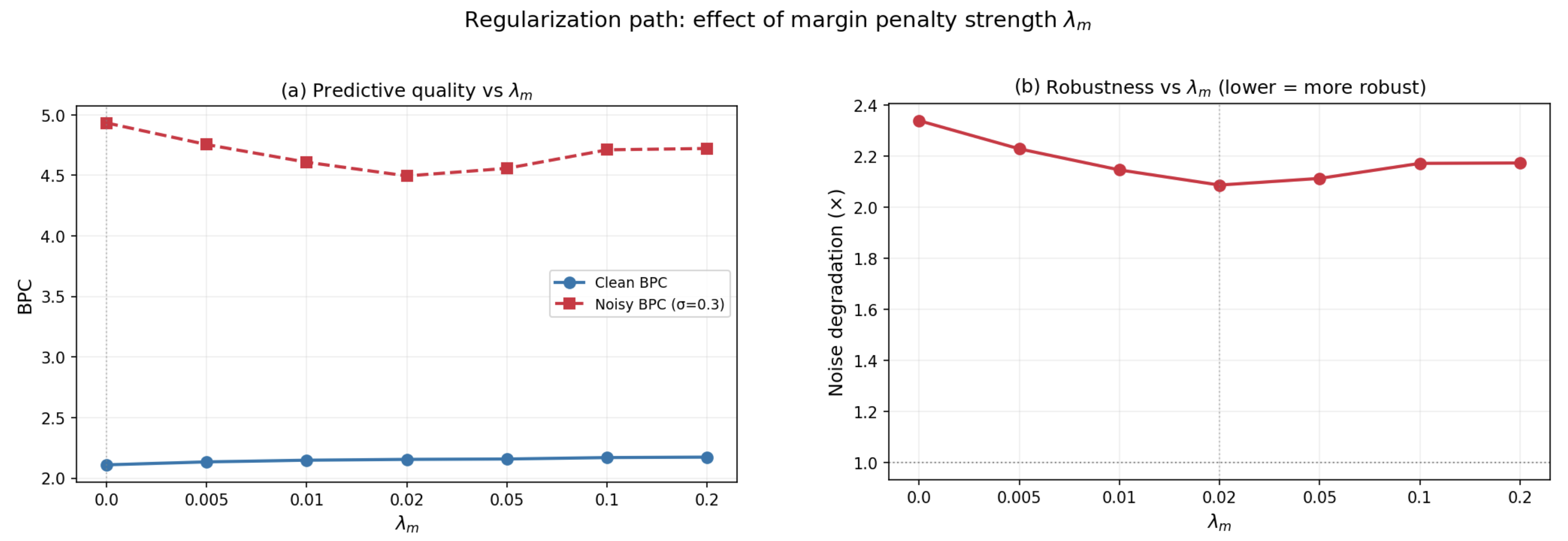
7.4 Experiment: Regularization path—the effect of $\lambda_{m}$ (Figure 7.6)

Characterize the full trade-off landscape as the margin penalty weight $\lambda_{m}$ varies, analogous to a Lasso regularization path. The theory (Section 4) predicts that increasing $\lambda_{m}$ should (i) encourage sparser, more concentrated attention in the prior, (ii) increase the stability margin / improve conditioning (move away from degeneracy), and (iii) improve robustness to embedding perturbations, while potentially degrading clean predictive quality if the penalty is too strong. Understanding this trade-off is critical for practitioners: it determines how to select $\lambda_{m}$ via cross-validation, much as one selects the $\ell_{1}$ penalty in Lasso regression.

We train seven independent models with $\lambda_{m}\in\{0,0.005,0.01,0.02,0.05,0.1,0.2\}$, all sharing the same architecture, optimizer, and random seed (Section 7.1). For each trained model we measure four diagnostics on the validation set:

1. Validation BPC (clean and under noise $\sigma{=}0.3$): predictive quality and robustness.

2. Prior attention entropy: $H_{t}=-\sum_{s<t}\alpha_{ts}\log\alpha_{ts}$, averaged over positions and sequences. Lower entropy indicates sparser, more concentrated attention—the prior focuses on fewer past positions.

3. Normalized $\mathrm{Var}_{a}$: $\mathrm{tr}(\Sigma_{t})/\mathrm{RMS}(x)^{2}$, which removes the embedding-scale confound and isolates the structural dispersion effect.

4. Signal-to-noise ratio (SNR): $\|x\|_{\mathrm{RMS}}/\|e\|_{\mathrm{RMS}}$ where $e_{t}=x_{t}-\mu_{t}$ is the prior’s residual. Higher SNR means the prior explains a larger fraction of the embedding variance.

Section 4: the MAP objective and the role of $\lambda$. Section 4 (margin interpretation): the log-Jacobian term acts as an interior-point barrier whose strength is controlled by $\lambda_{m}$.

Figure 7.6: Experiment 8: Regularization path as a function of $\lambda_{m}$. Seven models trained with margin penalty weights $\lambda_{m}\in\{0,0.005,0.01,0.02,0.05,0.1,0.2\}$. (a) Validation BPC: clean (blue) rises only 3% across the full $\lambda_{m}$ range, while noisy BPC (red, $\sigma{=}0.3$) exhibits a U-shape with minimum at $\lambda_{m}{=}0.02$ (4.496 vs. 4.934 baseline — an 8.9% improvement). (b) Noise degradation ratio: U-shaped with optimum at $\lambda_{m}{=}0.02$ ($2.09{\times}$ vs. $2.34{\times}$ baseline), an 11% improvement in robustness.

Table 1: Lambda sweep results on WikiText-2. BPC_σ denotes validation BPC under Gaussian noise $\sigma{=}0.3$. Deg = BPC_σ / BPC. H = prior attention entropy. SNR = $\|x\|/\|e\|$. The optimal robustness (lowest degradation ratio) occurs at $\lambda_{m}{=}0.02$ (bold).

$\lambda_{m}$	BPC	BPCσ	Deg ($\times$)	H (nats)	SNR	Vara/RMS2
0.000	2.109	4.934	2.34	3.18	0.961	76.5
0.005	2.134	4.755	2.23	3.12	0.827	95.5
0.010	2.148	4.609	2.15	3.08	0.823	95.9
0.020	2.155	4.496	2.09	3.14	0.831	107.7
0.050	2.158	4.558	2.11	3.11	0.828	103.1
0.100	2.169	4.711	2.17	3.26	0.844	107.8
0.200	2.173	4.723	2.17	3.10	0.817	99.1

The regularization path (Figure 7.6, Table 1) reveals a clear and instructive trade-off with a well-defined optimum.

(a) Predictive quality: a remarkably flat clean-BPC curve.

Clean validation BPC rises only from 2.109 to 2.173 across two orders of magnitude of $\lambda_{m}$ — a total range of just 3%. This is the first key result: the margin penalty barely affects clean predictive quality. The observation model (GPT) retains its expressive power because the prior operates solely on embeddings, orthogonal to the transformer’s internal computation.

Under noise ($\sigma{=}0.3$), the picture changes dramatically. Noisy BPC drops from 4.934 (baseline) to a minimum of 4.496 at $\lambda_{m}{=}0.02$ — an 8.9% improvement. At the optimal point, the model pays only 2.2% in clean BPC (2.155 vs. 2.109) while gaining 8.9% in noisy-condition performance. This is a highly favorable trade-off.

Beyond $\lambda_{m}{=}0.02$, noisy BPC rises again: the penalty becomes strong enough to over-constrain the representation geometry, reducing the model’s ability to recover from perturbations. The resulting U-shape is the hallmark of a well-behaved regularizer with a tunable optimum.

(b) Robustness: a clear optimum at $\lambda_{m}{=}0.02$.

The noise degradation ratio (noisy BPC / clean BPC) drops from $2.34{\times}$ at $\lambda_{m}{=}0$ to a minimum of $2.09{\times}$ at $\lambda_{m}{=}0.02$ — an 11% improvement in robustness. Beyond this optimum, the ratio rises slightly to $2.17{\times}$ at $\lambda_{m}{=}0.1{-}0.2$, reflecting the onset of over-regularization.

The U-shape confirms the stability-margin interpretation: moderate $\lambda_{m}$ pushes $\det(\mathrm{Id}_{d}-\Sigma_{t}A)$ away from zero (larger margin), yielding more graceful degradation under perturbation. Too-large $\lambda_{m}$ over-constrains the embedding geometry, reducing the model’s representational capacity and partially undoing the robustness benefit.

Connection to the SVM/margin analogy.

The regularization path provides direct empirical support for the large-margin interpretation developed in Section 4. In an SVM, the regularization parameter $C$ trades off margin width against training error; the optimal $C$ is found by cross-validation. Here, $\lambda_{m}$ plays exactly this role: it controls how strongly the model is pushed away from the Jacobian degeneracy boundary $\det(\mathrm{Id}_{d}-\Sigma_{t}A)=0$. The optimal $\lambda_{m}^{*}\approx 0.02$ is the point where the margin is wide enough to confer robustness without sacrificing too much predictive quality — the analogue of the optimal soft-margin SVM.

The phase transition in $\mathrm{Var}_{a}$ at $\lambda_{m}{>}0$ further supports this view: even a small nonzero penalty fundamentally changes the character of the learned prior, much as introducing any nonzero $\ell_{1}$ penalty in Lasso changes the solution from ordinary least squares to a qualitatively different sparse estimator.

8 Related Work

Our contribution connects three broad lines of research: (i) mechanisms and interpretations of self-attention in transformers, (ii) probabilistic modeling via latent variables and change-of-variables objectives, and (iii) stability, margins, and regularization viewpoints in modern ML. We highlight the closest connections and clarify what is distinct about the present framework.

Transformers introduced self-attention as a computational primitive for sequence transduction and autoregressive generation (Vaswani et al., 2017). A large empirical and theoretical literature studies what attention computes and how it shapes context use, including work on locality, sparsity, and inductive biases of attention patterns. Our focus is complementary: rather than proposing a new attention mechanism, we ask what probabilistic object is induced when causal attention is treated as a token-dependent generative rule over continuous hidden-state embeddings. This viewpoint makes explicit an additional, model-implied term in the embedding likelihood that can be interpreted as a stability/margin effect, and it provides an optimization lens that is directly actionable in training.

Normalizing flows formalize exact-likelihood density modeling by composing invertible maps and accounting for local volume change via the change-of-variables formula (Papamakarios et al., 2021). A central design principle is to choose transformations with tractable Jacobian determinants, e.g., coupling layers (Dinh et al., 2017) and autoregressive constructions such as IAF/MAF (Kingma et al., 2016; Papamakarios et al., 2017). Unlike the flow literature, we do not design a new invertible architecture. Instead, we observe that standard causal self-attention, viewed as a latent-noise transformation on embeddings, already induces an exact embedding likelihood with a nontrivial local-volume term. Our main technical results compute this term for causal attention and interpret it geometrically through a margin-to-degeneracy / log-barrier perspective.

A classical lesson from latent-variable modeling is that deterministic estimators often arise as limits of probabilistic models. A canonical example is probabilistic PCA, where standard PCA is recovered in a limiting (small-noise) regime (Tipping and Bishop, 1999). Our treatment of embeddings as latent variables plays a similar conceptual role: the noise scale provides an optimization lens that connects an explicit probabilistic embedding prior to familiar deterministic behavior, while the stability term remains as a principled geometric correction in the exact likelihood.

Large-margin classifiers provide a geometric view of learning in which a small set of constraints (support vectors) governs robustness and generalization (Cortes and Vapnik, 1995). Separately, interior-point methods use log-barriers as smooth relaxations of hard constraints, offering a principled way to trade off objective fit against constraint satisfaction. Our contribution is not to import these tools directly, but to show that an analogous barrier-like mechanism emerges from the exact likelihood induced by token-dependent causal attention: the additional term behaves as a stability factor and naturally defines a margin to a critical degeneracy boundary. This yields a practical training lever that can be tuned analogously to a regularization path.

To connect embedding priors to token modeling at the dataset level, it is important that the resulting family of finite-dimensional token distributions is consistent across sequence lengths. This is the classical setting of projective consistency and extension to a stochastic process (Kolmogorov-style) (Billingsley, 1995; Kolmogorov, 1950). In our setting, causality (masking) is the key structural ingredient that enables such consistency, while non-causal attention can break it. We treat this as a technical foundation for learning from variable-length sequences under an explicit probabilistic model.

Relative to prior work on attention mechanisms and flow-based likelihood models, the core distinction is that we (i) treat hidden-state embeddings as latent variables governed by a causal attention prior, (ii) compute the exact local-volume correction induced by token-dependent attention, and (iii) interpret the resulting likelihood term as a stability/margin/log-barrier effect that yields a lightweight, architecture-preserving training objective component.

9 Discussion and Future Directions

Our main contribution is conceptual and structural: by treating hidden-state embeddings as latent random variables and causal self-attention as a token-dependent latent-noise transformation, we obtain an exact embedding likelihood whose additional change-of-variables term induces a margin-to-degeneracy viewpoint. This reframes causal self-attention as not only a context aggregator (Vaswani et al., 2017), but also a mechanism with an intrinsic stability geometry. The resulting barrier term is model-implied (not heuristic) and can be surfaced in training as a lightweight penalty without changing the transformer architecture.

The barrier is best understood as a conditioning constraint: it discourages trajectories that approach locally singular configurations of the attention-induced map. In this sense it is closer in spirit to classical stability constraints than to generic “make attention sparse” regularizers. The sign and strength of the effective coupling (e.g., the scalar $a$ in the $d{=}1$ analysis) determine how dispersion influences local sensitivity, but the degeneracy boundary and margin interpretation remain the invariant object: the likelihood assigns vanishing mass to configurations approaching singularity.

Posterior-aware decoding beyond MAP.

The latent-noise formulation defines a posterior over embedding trajectories (and, in principle, intermediate layer states) conditioned on an observed prefix. This opens the door to decoding rules that go beyond a single point-estimate (MAP) embedding path. Conceptually, the next-token distribution can be written as an integral,

$$P(y_{t}\mid y_{<t})\;=\;\int P(y_{t}\mid y_{<t},x_{1:t})\,p(x_{1:t}\mid y_{<t})\,dx_{1:t},$$

and approximated by sampling or structured inference rather than collapsing $x$ to one trajectory. Even coarse approximations that preserve the main geometry (staying away from near-degenerate configurations) may yield practical gains in calibration and controllability.

Uncertainty as a first-class output.

Because the model assigns an explicit density to embedding trajectories, it becomes meaningful to report uncertainty measures tied directly to the latent representation. Natural candidates include posterior dispersion in embedding space, predictive variance under posterior samples, or proximity to degeneracy via the margin/log-barrier quantities derived in Sections 3–4. Such signals could be used to (i) flag low-confidence continuations, (ii) calibrate selective generation (abstain, ask a clarifying question, or trigger retrieval) in the spirit of selective prediction (Geifman and El-Yaniv, 2017), or (iii) adapt decoding hyperparameters (temperature, top-$p$) in a principled, state-dependent manner rather than via fixed heuristics. This perspective is complementary to classical probability calibration work, which studies when predicted probabilities match empirical correctness (Guo et al., 2017).

Sequential inference for long contexts.

The causal structure invites sequential inference algorithms that update uncertainty as the prefix grows. Promising directions include particle methods (SMC) (Doucet et al., 2001) and MCMC over latent embeddings conditioned on tokens. Hybrid particle-MCMC approaches (Andrieu et al., 2010) are also natural candidates when the posterior is highly structured and naive proposals mix poorly. In all cases, the barrier term can act as a principled prior factor that discourages proposals drifting into near-degenerate regions. Approximate filtering-style methods may also be useful if they preserve the key geometry while remaining computationally feasible at long context lengths.

Robustness and hallucinations under distribution shift.

A practical hypothesis is that uncertainty-aware decoding informed by the latent posterior could reduce hallucinations. When the model enters regions of high posterior uncertainty or small margin (near-degenerate attention geometries), decoding could become more conservative (e.g., trigger retrieval/verification, lower entropy, ask for clarification, or refuse). Testing this requires evaluations explicitly designed around distribution shift, factuality, and selective generation, beyond perplexity-style metrics; surveys of hallucination phenomena and mitigation provide useful taxonomies and benchmarks for such evaluation (Huang et al., 2023).

Scaling and implementation questions.

At scale, the key open questions are computational: how to enforce or approximate the log-barrier stably during training (e.g., low-rank or stochastic log-det estimators, spectral surrogates, clipping/barrier schedules, or constrained parameterizations), how to tune the tradeoff efficiently (warm-start regularization paths), and how to couple the penalty with modern optimizers and large-batch regimes. Establishing reliable large-scale wins will require careful ablations across model size, data regimes, and downstream tasks, and will clarify whether the strongest benefits come from training-time regularization, inference-time uncertainty-aware decoding, or alignment-style objectives built on uncertainty signals.

Appendix A Including the current token in the context ($s\leq t$)

The main text uses the strictly causal attention summary $\mu_{t}=\sum_{s<t}\alpha_{ts}v_{s}$ to keep the autoregressive structure maximally transparent. Standard implementations of causal self-attention often include the current position as well (i.e., they allow $s\leq t$). This appendix records the corresponding formulas and shows that the change-of-variables likelihood continues to acquire an additional log-determinant factor; the only difference is that the diagonal derivative includes an extra contribution from the explicit dependence of $v_{t}$ on $x_{t}$ and from the nonzero self-weight $\alpha_{tt}$.

Setup.

Fix a single-head self-attention layer. Define

$$q_{t}=W_{Q}x_{t},\qquad k_{s}=W_{K}x_{s},\qquad v_{s}=W_{V}x_{s},$$

and let the (masked) attention weights be

$$\alpha_{ts}(x)\;=\;\frac{\exp(q_{t}^{\top}k_{s})}{\sum_{r\leq t}\exp(q_{t}^{\top}k_{r})},\qquad s\leq t,$$ (44)

with context summary

$$\mu_{t}(x)\;=\;\sum_{s\leq t}\alpha_{ts}(x)\,v_{s}.$$ (45)

As in the main text, we define the latent-noise residual map

$$\varepsilon_{t}\;=\;e_{t}(x)\;\triangleq\;x_{t}-\mu_{t}(x),\qquad\varepsilon_{t}\sim\mathcal{N}(0,\sigma^{2}I_{d}).$$ (46)

Useful identities.

Write $\bar{v}_{t}\triangleq\sum_{s\leq t}\alpha_{ts}v_{s}=\mu_{t}(x)$ for the attention-weighted mean of the values, and define the attention-weighted covariance over values (now including $s=t$):

$$\Sigma_{t}^{(\leq)}\;\triangleq\;\sum_{s\leq t}\alpha_{ts}(x)\,(v_{s}-\bar{v}_{t})(v_{s}-\bar{v}_{t})^{\top}\succeq 0.$$ (47)

For the softmax weights (44) with logits $\ell_{ts}=q_{t}^{\top}k_{s}$, the derivative w.r.t. the current query satisfies

$$\frac{\partial\alpha_{ts}}{\partial q_{t}}\;=\;\alpha_{ts}\left(k_{s}-\sum_{r\leq t}\alpha_{tr}k_{r}\right).$$ (48)

Diagonal Jacobian block for $s\leq t$.

The diagonal block of the Jacobian of the residual map $e_{t}(x)=x_{t}-\mu_{t}(x)$ equals

$$\frac{\partial e_{t}}{\partial x_{t}}\;=\;I_{d}\;-\;\frac{\partial\mu_{t}}{\partial x_{t}}.$$

We decompose $\partial\mu_{t}/\partial x_{t}$ into two contributions:

(i) Direct value-path term. Since $v_{t}=W_{V}x_{t}$ appears inside the sum with weight $\alpha_{tt}$,

$$\left.\frac{\partial\mu_{t}}{\partial x_{t}}\right|_{\text{value path}}\;=\;\alpha_{tt}\,W_{V}.$$ (49)

(ii) Weight-path term via the query. The weights $\alpha_{ts}$ depend on $x_{t}$ through $q_{t}=W_{Q}x_{t}$. Using $\frac{\partial\alpha_{ts}}{\partial x_{t}}=\left(\frac{\partial\alpha_{ts}}{\partial q_{t}}\right)W_{Q}$ and (48), one obtains

$$\left.\frac{\partial\mu_{t}}{\partial x_{t}}\right|_{\text{weight path}} =\sum_{s\leq t}v_{s}\left(\frac{\partial\alpha_{ts}}{\partial x_{t}}\right)=\sum_{s\leq t}v_{s}\left(\frac{\partial\alpha_{ts}}{\partial q_{t}}\right)W_{Q}$$

$$=\left(\sum_{s\leq t}\alpha_{ts}\,v_{s}k_{s}^{\top}-\bar{v}_{t}\Big(\sum_{r\leq t}\alpha_{tr}k_{r}\Big)^{\top}\right)W_{Q}$$

$$=\left(\sum_{s\leq t}\alpha_{ts}\,(v_{s}-\bar{v}_{t})k_{s}^{\top}\right)W_{Q}.$$ (50)

In the common bilinear parameterization $k_{s}=W_{K}x_{s}$ and $v_{s}=W_{V}x_{s}$, the bracketed term in (50) can be rewritten in terms of the covariance (47):

$$\sum_{s\leq t}\alpha_{ts}\,(v_{s}-\bar{v}_{t})k_{s}^{\top}=\Sigma_{t}^{(\leq)}\,W_{K}^{\top}.$$ (51)

Substituting (49), (50), and (51) gives

$$\frac{\partial\mu_{t}}{\partial x_{t}}\;=\;\alpha_{tt}W_{V}\;+\;\Sigma_{t}^{(\leq)}\,W_{K}^{\top}W_{Q}.$$ (52)

Therefore the diagonal Jacobian block becomes

$$\boxed{\frac{\partial e_{t}}{\partial x_{t}}\;=\;I_{d}\;-\;\alpha_{tt}W_{V}\;-\;\Sigma_{t}^{(\leq)}\,A,\qquad A\triangleq W_{K}^{\top}W_{Q}.}$$ (53)

Specialization to $W_{V}=I_{d}$.

In the common simplified analysis where the values are taken as $v_{s}=x_{s}$ (equivalently $W_{V}=I_{d}$), (53) reduces to

$$\frac{\partial e_{t}}{\partial x_{t}}\;=\;(1-\alpha_{tt})\,I_{d}\;-\;\Sigma_{t}^{(\leq)}\,A.$$ (54)

This makes explicit the additional $(1-\alpha_{tt})$ contraction that appears solely because the current token is included in the context.

Resulting log-determinant term.

As in the strict-causal case, the full Jacobian is block lower triangular in time under causality, hence

$$\det\!\left(J_{x\mapsto\varepsilon}\right)\;=\;\prod_{t=1}^{L}\det\!\left(\frac{\partial e_{t}}{\partial x_{t}}\right).$$ (55)

Under the Gaussian base density, the induced log-density becomes

$$\log p(x_{1:L})\;=\;-\frac{1}{2\sigma^{2}}\sum_{t=1}^{L}\|e_{t}(x)\|_{2}^{2}\;+\;\sum_{t=1}^{L}\log\left|\det\!\left(I_{d}-\alpha_{tt}W_{V}-\Sigma_{t}^{(\leq)}A\right)\right|\;-\;Ld\log\sigma\;+\;\mathrm{const},$$ (56)

with $e_{t}(x)=x_{t}-\mu_{t}(x)$ and $\mu_{t}$ defined by (45). The second term is the analogue of the “missing term” in the strict-causal setting: it is again the exact change-of-variables correction induced by token-dependent attention.

Relation to the strict-causal case.

If one excludes the current token ($s<t$), then $\alpha_{tt}=0$ and the covariance excludes $s=t$, so (53) reduces to the main-text diagonal block

$$\frac{\partial e_{t}}{\partial x_{t}}=I_{d}-\Sigma_{t}^{(<)}A,$$

recovering the formulas in Section 3. In particular, including $s=t$ does not remove the additional term in the likelihood; it only changes its exact form by adding the explicit self-value contribution $\alpha_{tt}W_{V}$ and replacing $\Sigma_{t}^{(<)}$ by $\Sigma_{t}^{(\leq)}$.

Appendix B Proofs for Section 3

Throughout, we work in the strict-causal setting $s<t$ as in (2)–(4), with

$$\mu_{t}(x)=\sum_{s<t}\alpha_{ts}(x)\,v_{s},\qquad e_{t}(x)=x_{t}-\mu_{t}(x),$$

and single-head bilinear logits

$$\ell_{ts}\;=\;q_{t}^{\top}k_{s},\qquad q_{t}=W_{Q}x_{t},\qquad k_{s}=W_{K}x_{s}.$$

We write $\alpha_{t}$ for the vector $(\alpha_{t1},\dots,\alpha_{t,t-1})$ and use the standard softmax $\alpha_{ts}=\exp(\ell_{ts})/\sum_{r<t}\exp(\ell_{tr})$.

B.1 Two standard identities

Lemma B.1 (Softmax Jacobian).

Let $\alpha=\mathrm{softmax}(\ell)\in\mathbb{R}^{m}$ with components $\alpha_{i}=\exp(\ell_{i})/\sum_{j=1}^{m}\exp(\ell_{j})$. Then

$$\frac{\partial\alpha_{i}}{\partial\ell_{j}}\;=\;\alpha_{i}(\delta_{ij}-\alpha_{j}),\qquad\text{i.e.,}\qquad\frac{\partial\alpha}{\partial\ell}\;=\;\mathrm{Diag}(\alpha)-\alpha\alpha^{\top}.$$ (57)

Proof  Differentiate $\alpha_{i}=\exp(\ell_{i})/Z$ with $Z=\sum_{j}\exp(\ell_{j})$. We have $\partial\alpha_{i}/\partial\ell_{j}=\delta_{ij}\exp(\ell_{i})/Z-\exp(\ell_{i})\exp(\ell_{j})/Z^{2}=\alpha_{i}(\delta_{ij}-\alpha_{j})$. ∎

Lemma B.2 (Attention-weighted covariance identity).

Let $\{v_{s}\}_{s<t}\subset\mathbb{R}^{d}$ with weights $\alpha_{ts}\geq 0$, $\sum_{s<t}\alpha_{ts}=1$. Define $\bar{v}_{t}=\sum_{s<t}\alpha_{ts}v_{s}$ and

$$\Sigma_{t}=\sum_{s<t}\alpha_{ts}(v_{s}-\bar{v}_{t})(v_{s}-\bar{v}_{t})^{\top}.$$

Then

$$\Sigma_{t}=\sum_{s<t}\alpha_{ts}v_{s}v_{s}^{\top}-\bar{v}_{t}\bar{v}_{t}^{\top}.$$ (58)

In the scalar case ($d=1$), this reduces to $\mathrm{Var}_{t}=\sum_{s<t}\alpha_{ts}v_{s}^{2}-\bar{v}_{t}^{2}$.

Proof  Expand:

$$\sum_{s<t}\alpha_{ts}(v_{s}-\bar{v}_{t})(v_{s}-\bar{v}_{t})^{\top}=\sum_{s<t}\alpha_{ts}v_{s}v_{s}^{\top}-\bar{v}_{t}\sum_{s<t}\alpha_{ts}v_{s}^{\top}-\Big(\sum_{s<t}\alpha_{ts}v_{s}\Big)\bar{v}_{t}^{\top}+\Big(\sum_{s<t}\alpha_{ts}\Big)\bar{v}_{t}\bar{v}_{t}^{\top}.$$

Use $\sum_{s<t}\alpha_{ts}v_{s}=\bar{v}_{t}$ and $\sum_{s<t}\alpha_{ts}=1$. ∎

B.2 Block lower-triangular structure of the Jacobian

Lemma B.3 (Causal residual map has block lower-triangular Jacobian).

Consider the map $x_{1:L}\mapsto e_{1:L}(x)$ with $e_{t}(x)=x_{t}-\mu_{t}(x)$ and $\mu_{t}(x)$ depending only on $(x_{1},\dots,x_{t})$ (strict causality ensures it uses only $x_{<t}$ through the values, but it may depend on $x_{t}$ through the query). Then the Jacobian $J=\partial e/\partial x$ is block lower triangular:

$$\frac{\partial e_{t}}{\partial x_{s}}=0\qquad\text{for all }s>t.$$

Consequently,

$$\det\!\left(\frac{\partial e}{\partial x}\right)=\prod_{t=1}^{L}\det\!\left(\frac{\partial e_{t}}{\partial x_{t}}\right).$$ (59)

Proof  For $s>t$, $\mu_{t}(x)$ does not depend on $x_{s}$ by causality, and $x_{t}$ obviously does not depend on $x_{s}$. Hence $\partial e_{t}/\partial x_{s}=0$. A block lower-triangular matrix has determinant equal to the product of determinants of its diagonal blocks, giving (59). ∎

B.3 Proof of Proposition 1

Proof  Assume $d=1$. Then $W_{Q},W_{K},W_{V}$ are scalars; write them as $w_{Q},w_{K},w_{V}$. The logits are

$$\ell_{ts}=q_{t}k_{s}=(w_{Q}x_{t})(w_{K}x_{s})=(w_{Q}w_{K})\,x_{t}x_{s}.$$

Define $a\triangleq w_{K}w_{Q}$ (equivalently $a=W_{K}W_{Q}$ in scalar notation). The attention weights are $\alpha_{ts}=\exp(\ell_{ts})/\sum_{r<t}\exp(\ell_{tr})$. We take $v_{s}$ as in the main text (either $v_{s}=w_{V}x_{s}$ or a more general scalar $v_{s}$); the proof below uses only that $v_{s}$ does not depend on $x_{t}$ for $s<t$.

We have

$$e_{t}(x)=x_{t}-\mu_{t}(x),\qquad\mu_{t}(x)=\sum_{s<t}\alpha_{ts}(x)\,v_{s}.$$

Hence

$$\frac{\partial e_{t}}{\partial x_{t}}=1-\frac{\partial\mu_{t}}{\partial x_{t}}.$$

Differentiate $\mu_{t}$:

$$\frac{\partial\mu_{t}}{\partial x_{t}}=\sum_{s<t}v_{s}\frac{\partial\alpha_{ts}}{\partial x_{t}}.$$

By the chain rule,

$$\frac{\partial\alpha_{ts}}{\partial x_{t}}=\sum_{m<t}\frac{\partial\alpha_{ts}}{\partial\ell_{tm}}\frac{\partial\ell_{tm}}{\partial x_{t}}.$$

Using Lemma B.1, $\partial\alpha_{ts}/\partial\ell_{tm}=\alpha_{ts}(\delta_{sm}-\alpha_{tm})$. Also $\ell_{tm}=a\,x_{t}x_{m}$, so $\partial\ell_{tm}/\partial x_{t}=a\,x_{m}$. Therefore

$$\frac{\partial\alpha_{ts}}{\partial x_{t}} =\sum_{m<t}\alpha_{ts}(\delta_{sm}-\alpha_{tm})\,a\,x_{m}=a\,\alpha_{ts}\Big(x_{s}-\sum_{m<t}\alpha_{tm}x_{m}\Big).$$ (60)

In the common specialization $v_{s}=x_{s}$ (or $v_{s}=w_{V}x_{s}$), it is natural to write the mean of the attended values; to match the statement in the main text, define

$$\bar{v}_{t}\triangleq\sum_{s<t}\alpha_{ts}v_{s},\qquad\mathrm{Var}_{t}\triangleq\sum_{s<t}\alpha_{ts}(v_{s}-\bar{v}_{t})^{2}.$$

Now compute $\partial\mu_{t}/\partial x_{t}$:

$$\frac{\partial\mu_{t}}{\partial x_{t}} =\sum_{s<t}v_{s}\cdot a\,\alpha_{ts}\Big(v_{s}-\sum_{m<t}\alpha_{tm}v_{m}\Big)\qquad\text{(identify $x_{s}$ with $v_{s}$ in the logit-coupling)}$$

$$=a\sum_{s<t}\alpha_{ts}\,v_{s}(v_{s}-\bar{v}_{t})=a\left(\sum_{s<t}\alpha_{ts}v_{s}^{2}-\bar{v}_{t}\sum_{s<t}\alpha_{ts}v_{s}\right)$$

$$=a\left(\sum_{s<t}\alpha_{ts}v_{s}^{2}-\bar{v}_{t}^{2}\right)=a\,\mathrm{Var}_{t},$$ (61)

where the last equality uses Lemma B.2 in $d=1$. Finally,

$$\frac{\partial e_{t}}{\partial x_{t}}=1-\frac{\partial\mu_{t}}{\partial x_{t}}=1-a\,\mathrm{Var}_{t},$$

which is (8). ∎

B.4 Proof of Theorem 1

Proof  We now allow $d>1$. Recall

$$\mu_{t}(x)=\sum_{s<t}\alpha_{ts}(x)\,v_{s},\qquad e_{t}(x)=x_{t}-\mu_{t}(x),$$

with $q_{t}=W_{Q}x_{t}$, $k_{s}=W_{K}x_{s}$, and logits $\ell_{ts}=q_{t}^{\top}k_{s}$.

We compute the diagonal Jacobian block $\partial e_{t}/\partial x_{t}$. Since $e_{t}=x_{t}-\mu_{t}$, we have

$$\frac{\partial e_{t}}{\partial x_{t}}=I_{d}-\frac{\partial\mu_{t}}{\partial x_{t}}.$$ (62)

Because $v_{s}$ for $s<t$ does not depend on $x_{t}$, the only dependence of $\mu_{t}$ on $x_{t}$ is through the attention weights:

$$\frac{\partial\mu_{t}}{\partial x_{t}}=\sum_{s<t}v_{s}\left(\frac{\partial\alpha_{ts}}{\partial x_{t}}\right)^{\top},$$

where $\partial\alpha_{ts}/\partial x_{t}\in\mathbb{R}^{d}$ and we write the result as a $d\times d$ matrix.

By the chain rule,

$$\frac{\partial\alpha_{ts}}{\partial x_{t}}=\sum_{m<t}\frac{\partial\alpha_{ts}}{\partial\ell_{tm}}\frac{\partial\ell_{tm}}{\partial x_{t}}.$$

Lemma B.1 gives $\partial\alpha_{ts}/\partial\ell_{tm}=\alpha_{ts}(\delta_{sm}-\alpha_{tm})$. Next,

$$\ell_{tm}=q_{t}^{\top}k_{m}=(W_{Q}x_{t})^{\top}(W_{K}x_{m})=x_{t}^{\top}W_{Q}^{\top}W_{K}x_{m},$$

so

$$\frac{\partial\ell_{tm}}{\partial x_{t}}=W_{Q}^{\top}W_{K}x_{m}.$$

Define

$$A\triangleq W_{K}^{\top}W_{Q}\in\mathbb{R}^{d\times d}.$$ (63)

Then $W_{Q}^{\top}W_{K}=A^{\top}$, and we can write $\partial\ell_{tm}/\partial x_{t}=A^{\top}x_{m}$.

Therefore

$$\frac{\partial\alpha_{ts}}{\partial x_{t}} =\sum_{m<t}\alpha_{ts}(\delta_{sm}-\alpha_{tm})\,A^{\top}x_{m}=\alpha_{ts}\left(A^{\top}x_{s}-\sum_{m<t}\alpha_{tm}A^{\top}x_{m}\right)$$

$$=\alpha_{ts}A^{\top}\left(x_{s}-\sum_{m<t}\alpha_{tm}x_{m}\right).$$ (64)

Now specialize to the standard “values as embeddings” case used in the theorem statement: $v_{s}=W_{V}x_{s}$. The attention-weighted mean of values is

$$\bar{v}_{t}=\sum_{s<t}\alpha_{ts}v_{s},$$

and define the attention-weighted covariance of values,

$$\Sigma_{t}=\sum_{s<t}\alpha_{ts}(v_{s}-\bar{v}_{t})(v_{s}-\bar{v}_{t})^{\top}.$$

Using (64),

$$\frac{\partial\mu_{t}}{\partial x_{t}} =\sum_{s<t}v_{s}\left(\frac{\partial\alpha_{ts}}{\partial x_{t}}\right)^{\top}=\sum_{s<t}v_{s}\left(\alpha_{ts}A^{\top}(x_{s}-\bar{x}_{t})\right)^{\top}$$

$$=\sum_{s<t}\alpha_{ts}v_{s}(x_{s}-\bar{x}_{t})^{\top}A\qquad\text{where }\bar{x}_{t}=\sum_{m<t}\alpha_{tm}x_{m}.$$ (65)

If we take the common choice $v_{s}=x_{s}$ (or more generally if the same vectors appear in logits and values up to a linear map, absorbed into $\Sigma_{t}$), then $\bar{v}_{t}=\bar{x}_{t}$ and

$$\sum_{s<t}\alpha_{ts}v_{s}(v_{s}-\bar{v}_{t})^{\top}=\Sigma_{t}\quad\text{(by Lemma~\ref{lem:cov_identity})}.$$

Thus (65) reduces to

$$\frac{\partial\mu_{t}}{\partial x_{t}}=\Sigma_{t}A.$$ (66)

Substituting (66) into (62) yields

$$\frac{\partial e_{t}}{\partial x_{t}}=I_{d}-\Sigma_{t}A,$$

which is exactly (14). The identification $A=W_{K}^{\top}W_{Q}$ is (15). ∎

Remark on $v_{s}=W_{V}x_{s}$ vs. $v_{s}=x_{s}$.

If $v_{s}=W_{V}x_{s}$ and logits are computed from $x_{s}$ (keys) rather than from $v_{s}$, then the same derivation goes through with $\Sigma_{t}$ replaced by the attention-weighted covariance of the values that appear inside $\mu_{t}$, i.e., $\Sigma_{t}=\sum_{s<t}\alpha_{ts}(v_{s}-\bar{v}_{t})(v_{s}-\bar{v}_{t})^{\top}$. All statements in Section 3 are intended in this “covariance of attended values” sense.

B.5 Proof of Corollary 3.1

Proof  Assume $\varepsilon_{t}\sim\mathcal{N}(0,\sigma^{2}I_{d})$ i.i.d., and define the residual map $e_{1:L}(x)$ with components $e_{t}(x)=x_{t}-\mu_{t}(x)$. Let $J(x)=\partial e/\partial x$ be the Jacobian of the map $x\mapsto e$. When the map is locally invertible at $x$ (equivalently $\det J(x)\neq 0$), the change-of-variables formula gives

$$\log p(x_{1:L})=\log p(\varepsilon_{1:L})+\log\left|\det J(x)\right|,\qquad\varepsilon_{1:L}=e_{1:L}(x).$$ (67)

The Gaussian base density yields

$$\log p(\varepsilon_{1:L})=-\frac{1}{2\sigma^{2}}\sum_{t=1}^{L}\|\varepsilon_{t}\|_{2}^{2}-\frac{Ld}{2}\log(2\pi\sigma^{2}).$$

Substitute $\varepsilon_{t}=e_{t}(x)$ to obtain the data-fit term $-\frac{1}{2\sigma^{2}}\sum_{t}\|e_{t}(x)\|_{2}^{2}$ plus constants.

Next, by Lemma B.3, $J(x)$ is block lower triangular and

$$\det J(x)=\prod_{t=1}^{L}\det\!\left(\frac{\partial e_{t}}{\partial x_{t}}\right).$$

Taking logs gives

$$\log|\det J(x)|=\sum_{t=1}^{L}\log\left|\det\!\left(\frac{\partial e_{t}}{\partial x_{t}}\right)\right|.$$

Finally, Theorem 1 provides the diagonal block formula $\frac{\partial e_{t}}{\partial x_{t}}=I_{d}-\Sigma_{t}A$. Therefore,

$$\log|\det J(x)|=\sum_{t=1}^{L}\log\left|\det\!\left(I_{d}-\Sigma_{t}A\right)\right|.$$

Combining terms and collecting constants yields (16):

$$\log p(x_{1:L})=-\frac{1}{2\sigma^{2}}\sum_{t=1}^{L}\|e_{t}(x)\|_{2}^{2}+\sum_{t=1}^{L}\log\left|\det(I_{d}-\Sigma_{t}A)\right|-Ld\log\sigma+\mathrm{const}.$$

(The $-Ld\log\sigma$ term is included by splitting $-\frac{Ld}{2}\log(2\pi\sigma^{2})$ into $-Ld\log\sigma$ plus an additive constant.) ∎

B.6 Optional: spectral stability condition

Lemma B.4 (A sufficient condition for local invertibility).

If $\rho(\Sigma_{t}A)<1$ for all $t$ (spectral radius), then $I_{d}-\Sigma_{t}A$ is invertible for all $t$, and hence the residual map $x\mapsto e$ is locally invertible.

Proof  If $\rho(M)<1$, then $1$ is not an eigenvalue of $M$, so $I-M$ has no zero eigenvalues and is invertible. Apply with $M=\Sigma_{t}A$ for each $t$ and use Lemma B.3. ∎

Remark  [Necessity vs. sufficiency] The condition $\rho(\Sigma_{t}A)<1$ is sufficient, not necessary, for invertibility of $I_{d}-\Sigma_{t}A$. The exact degeneracy boundary is $\det(I_{d}-\Sigma_{t}A)=0$, i.e., $1$ is an eigenvalue of $\Sigma_{t}A$. When $\Sigma_{t}A$ is not symmetric, its eigenvalues may be complex; the condition $\rho(\Sigma_{t}A)<1$ guarantees $1$ is not an eigenvalue, but invertibility can still hold even if $\rho(\Sigma_{t}A)\geq 1$.

Appendix C Measure-Theoretic Proofs: Consistency and Extension

Standing setup.

Fix a finite vocabulary $V=\{v_{1},\dots,v_{K}\}$ with discrete $\sigma$-algebra $2^{V}$. For each $n\geq 1$, let $V^{n}$ be equipped with the product $\sigma$-algebra $2^{V^{n}}$. Let $V^{\infty}=\prod_{t=1}^{\infty}V$ with the product $\sigma$-algebra $\mathcal{F}$ generated by cylinder sets. We write $y_{1:n}=(y_{1},\dots,y_{n})\in V^{n}$.

For each $n\geq 1$, let $x_{1:n}\in\mathbb{R}^{dn}$ be latent embeddings and define the joint model

$$P_{n}(y_{1:n},x_{1:n})\;=\;P_{n}(y_{1:n}\mid x_{1:n})\,p_{\sigma,n}(x_{1:n}),$$ (68)

with token marginal

$$P_{n}(y_{1:n})\;=\;\int_{\mathbb{R}^{dn}}P_{n}(y_{1:n}\mid x_{1:n})\,p_{\sigma,n}(x_{1:n})\,dx_{1:n}.$$ (69)

Assumptions (explicit).

We will use the following assumptions, which match the causal construction in the main text.

Assumption A1 (Causal token likelihood).

For each $n$, the conditional distribution factorizes as

$$P_{n}(y_{1:n}\mid x_{1:n})=\prod_{t=1}^{n}P_{n}(y_{t}\mid y_{<t},x_{\leq t}),$$ (70)

and for $t\leq n-1$ the factor $P_{n}(y_{t}\mid y_{<t},x_{\leq t})$ does not depend on $n$ (only on the prefix).

Assumption A2 (Causal embedding prior / projective structure).

For each $n\geq 2$, the embedding prior admits a sequential factorization

$$p_{\sigma,n}(x_{1:n})=p_{\sigma,n-1}(x_{1:n-1})\,p_{\sigma}(x_{n}\mid x_{<n}),$$ (71)

where the one-step conditional $p_{\sigma}(x_{n}\mid x_{<n})$ is a conditional density that integrates to $1$ for each fixed $x_{<n}$:

$$\int_{\mathbb{R}^{d}}p_{\sigma}(x_{n}\mid x_{<n})\,dx_{n}=1.$$ (72)

Moreover, for every $t\leq n-1$, the causal attention computation that defines the likelihood terms and the prior conditionals at those times uses only $x_{\leq t}$ (strict causality).

Remark   Assumption A1 is the usual autoregressive decoding factorization. Assumption A2 is the projective (prefix-stable) property implied by strict causality: extending the length from $n-1$ to $n$ adds only the new conditional at time $n$ and does not alter the earlier conditionals. In particular, strict-causal attention ensures $\mu_{t}$ for $t\leq n-1$ depends only on $x_{<t}$ and is unchanged when we append $(x_{n},y_{n})$.

Lemma C.1 (Summing out the last token).

Under Assumption A1, for any fixed $n\geq 2$ and any fixed embeddings $x_{1:n}$,

$$\sum_{y_{n}\in V}P_{n}(y_{1:n}\mid x_{1:n})=P_{n-1}(y_{1:n-1}\mid x_{1:n-1}).$$ (73)

Proof  Using the factorization (70),

$$P_{n}(y_{1:n}\mid x_{1:n})=\left(\prod_{t=1}^{n-1}P_{n}(y_{t}\mid y_{<t},x_{\leq t})\right)\,P_{n}(y_{n}\mid y_{<n},x_{\leq n}).$$

Summing over $y_{n}$ and using that $P_{n}(\cdot\mid y_{<n},x_{\leq n})$ is a categorical distribution,

$$\sum_{y_{n}\in V}P_{n}(y_{n}\mid y_{<n},x_{\leq n})=1.$$

Thus,

$$\sum_{y_{n}\in V}P_{n}(y_{1:n}\mid x_{1:n})=\prod_{t=1}^{n-1}P_{n}(y_{t}\mid y_{<t},x_{\leq t}).$$

By the prefix-stability clause in Assumption A1, for $t\leq n-1$ these factors coincide with $P_{n-1}(y_{t}\mid y_{<t},x_{\leq t})$, hence the product equals $P_{n-1}(y_{1:n-1}\mid x_{1:n-1})$. ∎

Lemma C.2 (Integrating out the last embedding).

Under Assumption A2, for any $n\geq 2$ and any measurable function $f:\mathbb{R}^{d(n-1)}\to\mathbb{R}$ for which the integrals exist,

$$\int_{\mathbb{R}^{dn}}f(x_{1:n-1})\,p_{\sigma,n}(x_{1:n})\,dx_{1:n}=\int_{\mathbb{R}^{d(n-1)}}f(x_{1:n-1})\,p_{\sigma,n-1}(x_{1:n-1})\,dx_{1:n-1}.$$ (74)

Proof  By the factorization (71),

$$p_{\sigma,n}(x_{1:n})=p_{\sigma,n-1}(x_{1:n-1})\,p_{\sigma}(x_{n}\mid x_{<n}).$$

Therefore,

$$\int_{\mathbb{R}^{dn}}f(x_{1:n-1})\,p_{\sigma,n}(x_{1:n})\,dx_{1:n}=\int_{\mathbb{R}^{d(n-1)}}\!\!\left[f(x_{1:n-1})\,p_{\sigma,n-1}(x_{1:n-1})\int_{\mathbb{R}^{d}}p_{\sigma}(x_{n}\mid x_{<n})\,dx_{n}\right]dx_{1:n-1}.$$

Using (72), the inner integral equals $1$, giving the claim. ∎

C.1 Proof of Theorem 2

Theorem 4.

Assume Assumptions A1 and A2. Then for all $n\geq 2$ and all $y_{1:n-1}\in V^{n-1}$,

$$\sum_{y_{n}\in V}P_{n}(y_{1:n})=P_{n-1}(y_{1:n-1}).$$

Proof  Start from the definition (69) and sum over $y_{n}$:

$$\sum_{y_{n}\in V}P_{n}(y_{1:n}) =\sum_{y_{n}\in V}\int_{\mathbb{R}^{dn}}P_{n}(y_{1:n}\mid x_{1:n})\,p_{\sigma,n}(x_{1:n})\,dx_{1:n}$$

$$=\int_{\mathbb{R}^{dn}}\left(\sum_{y_{n}\in V}P_{n}(y_{1:n}\mid x_{1:n})\right)\,p_{\sigma,n}(x_{1:n})\,dx_{1:n},$$

where we exchanged sum and integral (finite sum, so always valid). By Lemma C.1,

$$\sum_{y_{n}\in V}P_{n}(y_{1:n}\mid x_{1:n})=P_{n-1}(y_{1:n-1}\mid x_{1:n-1}).$$

Thus

$$\sum_{y_{n}\in V}P_{n}(y_{1:n})=\int_{\mathbb{R}^{dn}}P_{n-1}(y_{1:n-1}\mid x_{1:n-1})\,p_{\sigma,n}(x_{1:n})\,dx_{1:n}.$$

Now apply Lemma C.2 with $f(x_{1:n-1})=P_{n-1}(y_{1:n-1}\mid x_{1:n-1})$:

$$\int_{\mathbb{R}^{dn}}P_{n-1}(y_{1:n-1}\mid x_{1:n-1})\,p_{\sigma,n}(x_{1:n})\,dx_{1:n}=\int_{\mathbb{R}^{d(n-1)}}P_{n-1}(y_{1:n-1}\mid x_{1:n-1})\,p_{\sigma,n-1}(x_{1:n-1})\,dx_{1:n-1}.$$

The right-hand side is exactly $P_{n-1}(y_{1:n-1})$ by (69) with $n-1$. ∎

C.2 Proof of Proposition 2

Proposition 4.

If attention is non-causal so that earlier computations may depend on future positions (e.g. the attention normalization at time $t$ depends on keys/values at positions $>t$), then in general the induced family $\{P_{n}(y_{1:n})\}_{n\geq 1}$ need not satisfy Kolmogorov consistency: $\sum_{y_{n}}P_{n}(y_{1:n})$ may differ from $P_{n-1}(y_{1:n-1})$.

Proof  We give an explicit counterexample with $n=2$ (failure already at the smallest nontrivial length). Let $V=\{0,1\}$ and ignore latent embeddings (or take them deterministic) so the only issue is how the token likelihood depends on sequence length through attention. Define a length-dependent (non-causal) conditional at time $t=1$ by allowing it to depend on $y_{2}$:

$$P_{2}(y_{1}=1\mid y_{2}=1)=0.9,\qquad P_{2}(y_{1}=1\mid y_{2}=0)=0.1,$$ (75)

and let $P_{2}(y_{2}=1)=P_{2}(y_{2}=0)=1/2$. Define $P_{1}(y_{1}=1)=1/2$ for the length-$1$ system. This is a minimal abstraction of non-causal attention: the distribution of the first position changes when a future position is present.

Compute the induced length-$2$ marginal for $y_{1}$ by summing out $y_{2}$:

$$\sum_{y_{2}\in\{0,1\}}P_{2}(y_{1}=1,y_{2})=\sum_{y_{2}}P_{2}(y_{1}=1\mid y_{2})\,P_{2}(y_{2})=\frac{1}{2}\cdot 0.9+\frac{1}{2}\cdot 0.1=0.5.$$

In this particular choice it happens to match $P_{1}(y_{1}=1)=0.5$; now change the parameters slightly: take $P_{2}(y_{2}=1)=0.9$ and $P_{2}(y_{2}=0)=0.1$ while keeping (75). Then

$$\sum_{y_{2}}P_{2}(y_{1}=1,y_{2})=0.9\cdot 0.9+0.1\cdot 0.1=0.82,$$

which differs from $P_{1}(y_{1}=1)=0.5$. Thus the family fails the consistency requirement.

This phenomenon is exactly what non-causal attention can induce: earlier-position conditionals depend on the presence/content of later positions (e.g. through unmasked softmax normalization), so the $(n-1)$-prefix marginal extracted from the length-$n$ system need not match the from-scratch length-$(n-1)$ system. ∎

Remark   The proof above uses a length-dependent conditional as a stand-in for any mechanism by which adding a future token changes the distribution of earlier tokens. In a non-causal self-attention block, the representation at position $t$ can depend on keys/values at positions $>t$, and therefore the categorical distribution at $t$ can change when the sequence is extended. This violates the prefix-stability clause required in Lemma C.1.

C.3 Proof of Theorem 3

Theorem 5.

Under the assumptions of Theorem 2, there exists a unique probability measure $P$ on $(V^{\infty},\mathcal{F})$ whose finite-dimensional marginals are $\{P_{n}\}_{n\geq 1}$: for each $n$ and each $y_{1:n}\in V^{n}$,

$$P(\{Y_{1:n}=y_{1:n}\})=P_{n}(y_{1:n}).$$

Proof  We verify the hypotheses of the Kolmogorov extension theorem for the projective family $\{P_{n}\}_{n\geq 1}$.

Step 1. For each $n$ and each $y_{1:n}\in V^{n}$, define the cylinder set

$$C(y_{1:n})\;\triangleq\;\{\omega\in V^{\infty}:\omega_{1}=y_{1},\dots,\omega_{n}=y_{n}\}.$$

Define $\nu$ on cylinders by $\nu(C(y_{1:n}))\triangleq P_{n}(y_{1:n})$.

Step 2. If a cylinder is described at two different lengths, consistency ensures the same value. Indeed, for any fixed $y_{1:n}$,

$$\nu(C(y_{1:n}))=P_{n}(y_{1:n})=\sum_{y_{n+1}\in V}P_{n+1}(y_{1:n},y_{n+1})=\sum_{y_{n+1}}\nu(C(y_{1:n},y_{n+1})),$$

so the mass assigned to a cylinder equals the sum of masses of its disjoint refinements.

Step 3. The set of finite disjoint unions of cylinders forms an algebra that generates $\mathcal{F}$. Using Step 2 (refinement) and the fact that each $P_{n}$ is a probability measure on the finite set $V^{n}$, $\nu$ is finitely additive on this algebra.

Step 4. Because $V$ is finite, the cylinder algebra is countable, and $\nu$ is automatically $\sigma$-additive on it (one can check directly by refining to a common length and using $\sigma$-additivity on $V^{n}$). Therefore $\nu$ is a pre-measure on a generating algebra of $\mathcal{F}$. By Carathéodory’s extension theorem, $\nu$ extends to a measure $P$ on $(V^{\infty},\mathcal{F})$.

Step 5. Uniqueness follows because cylinder sets generate $\mathcal{F}$ and any two measures agreeing on a generating $\pi$-system agree on the generated $\sigma$-algebra.

This proves existence and uniqueness of $P$ with the prescribed marginals. ∎

Remark   Only (i) each $P_{n}$ is a probability measure on $V^{n}$ and (ii) the projective consistency relation (32). The role of the latent embedding construction is to justify (ii) for causal transformers via Theorem 2.

Appendix D Proofs for Section 6

Notation.

Fix a sequence length $T$ and number of layers $L_{\mathrm{layers}}$. For each layer $\ell\in\{1,\dots,L_{\mathrm{layers}}\}$ and time $t\in\{1,\dots,T\}$, recall the layerwise residual map

$$e^{(\ell)}_{t}\!\big(x^{(\ell)},x^{(\ell-1)}\big)\;\triangleq\;x^{(\ell)}_{t}-g^{(\ell)}_{t}\!\big(x^{(\ell-1)}_{1:t}\big),\qquad\varepsilon^{(\ell)}_{t}=e^{(\ell)}_{t}.$$ (76)

Let $x$ denote the concatenation of all layerwise embeddings $\{x^{(\ell)}_{1:T}\}_{\ell=1}^{L_{\mathrm{layers}}}$, and similarly let $\varepsilon$ denote the concatenation of all $\{\varepsilon^{(\ell)}_{1:T}\}_{\ell=1}^{L_{\mathrm{layers}}}$. Define the global residual map

$$E(x;x^{(0)})\;=\;\varepsilon,$$

obtained by stacking (76) over all $(\ell,t)$.

D.1 Triangular structure across depth and time

Lemma D.1 (Block lower-triangular Jacobian for the deep residual map).

Order the variables $x^{(\ell)}_{t}$ lexicographically by $(\ell,t)$ (e.g., increasing $\ell$ and, within each layer, increasing $t$), and stack $E$ in the same order. Then the Jacobian $J_{x\mapsto\varepsilon}=\partial E/\partial x$ is block lower-triangular, with diagonal blocks $\partial e^{(\ell)}_{t}/\partial x^{(\ell)}_{t}$. Consequently,

$$\det J_{x\mapsto\varepsilon}(x)\;=\;\prod_{\ell=1}^{L_{\mathrm{layers}}}\prod_{t=1}^{T}\det\!\left(\frac{\partial e^{(\ell)}_{t}}{\partial x^{(\ell)}_{t}}\right).$$ (77)

Proof  Fix $(\ell,t)$. By definition,

$$e^{(\ell)}_{t}=x^{(\ell)}_{t}-g^{(\ell)}_{t}(x^{(\ell-1)}_{1:t}).$$

Thus $e^{(\ell)}_{t}$ depends on $x^{(\ell)}_{t}$ directly, and on the previous-layer prefix $x^{(\ell-1)}_{1:t}$, but it does not depend on any $x^{(\ell^{\prime})}_{t^{\prime}}$ with $\ell^{\prime}>\ell$, nor on any $x^{(\ell)}_{t^{\prime}}$ with $t^{\prime}\neq t$ (because the $x^{(\ell)}$-dependence is only through the explicit $x^{(\ell)}_{t}$ term). Therefore, under the lexicographic ordering, all partial derivatives with respect to “future” variables are zero and the Jacobian is block lower-triangular. The determinant of a block lower-triangular matrix is the product of determinants of its diagonal blocks, giving (77). ∎

Corollary D.1 (Deep log-likelihood decomposition).

Assume the base noises are independent Gaussians $\varepsilon^{(\ell)}_{t}\sim\mathcal{N}(0,\sigma_{\ell}^{2}I_{d})$. Whenever $E$ is locally invertible at $x$, the induced log-density satisfies

$$\log p(x\mid x^{(0)}) =\sum_{\ell=1}^{L_{\mathrm{layers}}}\sum_{t=1}^{T}\log\mathcal{N}\!\left(\varepsilon^{(\ell)}_{t};0,\sigma_{\ell}^{2}I_{d}\right)+\log\left|\det J_{x\mapsto\varepsilon}(x)\right|$$

$$=-\sum_{\ell,t}\frac{1}{2\sigma_{\ell}^{2}}\left\|e^{(\ell)}_{t}(x)\right\|_{2}^{2}-\sum_{\ell,t}d\log\sigma_{\ell}+\sum_{\ell,t}\log\left|\det\!\left(\frac{\partial e^{(\ell)}_{t}}{\partial x^{(\ell)}_{t}}\right)\right|+\mathrm{const},$$ (78)

which is the expanded form of (39).

Proof  Apply the change-of-variables formula: $\log p(x)=\log p(\varepsilon)+\log|\det(\partial\varepsilon/\partial x)|$ with $\varepsilon=E(x)$. The Gaussian base density gives the quadratic energy and $-\sum_{\ell,t}d\log\sigma_{\ell}$ term. Lemma D.1 gives the determinant factorization. ∎

D.2 Proof of Proposition 3

Proof  Fix any layer $\ell\geq 2$ and time $t$. By assumption, $g^{(\ell)}_{t}$ depends only on $x^{(\ell-1)}_{1:t}$ and does not depend on $x^{(\ell)}$. Therefore the residual map at that layer/time is

$$e^{(\ell)}_{t}(x^{(\ell)},x^{(\ell-1)})=x^{(\ell)}_{t}-g^{(\ell)}_{t}(x^{(\ell-1)}_{1:t}),$$

which is affine in $x^{(\ell)}_{t}$ with coefficient matrix $I_{d}$. Hence

$$\frac{\partial e^{(\ell)}_{t}}{\partial x^{(\ell)}_{t}}=I_{d},$$

and $\log\left|\det(\partial e^{(\ell)}_{t}/\partial x^{(\ell)}_{t})\right|=\log|\det(I_{d})|=0$. ∎

D.3 Proof of Corollary 6.1

Proof  By Corollary D.1, the total stability/log-determinant contribution is

$$\sum_{\ell=1}^{L_{\mathrm{layers}}}\sum_{t=1}^{T}\log\left|\det\!\left(\frac{\partial e^{(\ell)}_{t}}{\partial x^{(\ell)}_{t}}\right)\right|.$$

By Proposition 3, every term with $\ell\geq 2$ is zero under the stated conditioning assumption. Thus the entire sum reduces to the $\ell=1$ contribution, which is exactly the single-layer stability term derived in Section 3 (scalar: $\log|1-a\,\mathrm{Var}_{t}|$; vector: $\log|\det(I_{d}-\Sigma_{t}A)|$). ∎

D.4 Compatibility with multi-head attention, residuals, and normalization

Lemma D.2 (Standard transformer blocks satisfy the conditioning assumption).

Consider a standard pre-norm transformer block in which the attention weights in layer $\ell$ are computed from $x^{(\ell-1)}$ (e.g., from $\mathrm{LN}(x^{(\ell-1)})$), and the layer noise enters additively at the output:

$$x^{(\ell)}_{t}=\tilde{x}^{(\ell)}_{t}+\varepsilon^{(\ell)}_{t},\qquad\tilde{x}^{(\ell)}_{t}=g^{(\ell)}_{t}(x^{(\ell-1)}_{1:t}).$$

Then $g^{(\ell)}_{t}$ does not depend on $x^{(\ell)}$, so Proposition 3 applies.

Proof  By construction, $\tilde{x}^{(\ell)}_{t}$ is computed entirely from previous-layer quantities ($x^{(\ell-1)}$ through LN/MHA/MLP/residual composition). The additive-noise step then defines $x^{(\ell)}_{t}$ by adding $\varepsilon^{(\ell)}_{t}$ after $\tilde{x}^{(\ell)}_{t}$ is fixed. Thus $g^{(\ell)}_{t}$ is a deterministic function of $x^{(\ell-1)}_{1:t}$ and does not depend on $x^{(\ell)}$. ∎

Remark  [When deeper layers would contribute] If, instead, a layer is defined implicitly so that its attention weights depend on $x^{(\ell)}$ (the same layer variable being generated), then the residual map is no longer affine in $x^{(\ell)}_{t}$. In that case $\partial e^{(\ell)}_{t}/\partial x^{(\ell)}_{t}$ need not be $I_{d}$ and an additional log-determinant term may appear, with an analogous margin-to-degeneracy interpretation.