Stochastic Neural Networks for Quantum Devices

Abstract

This work presents a formulation to express and optimize stochastic neural networks as quantum circuits in gate-based quantum computing. Motivated by a classical perceptron, stochastic neurons are introduced and combined into a quantum neural network. The Kiefer-Wolfowitz algorithm in combination with simulated annealing is used for training the network weights. Several topologies and models are presented, including shallow fully connected networks, Hopfield Networks, Restricted Boltzmann Machines, Autoencoders and convolutional neural networks. We also demonstrate the combination of our optimized neural networks as an oracle for the Grover algorithm to realize a quantum generative AI model.

I Introduction

Neural networks are a common and increasingly important family of mathematical models consisting of connected neurons arranged in a large graphical model. They have shown impressive performance in a large series of applications, ranging from classification and regression [11], to data compression [70, 40], anomaly detection [62] or content generation [58]. They are commonly used for supervised, unsupervised [8], self-supervised [21], semi-supervised [24] or reinforcement learning [73]. Modern architectures, e.g. based on transformers [74] are used in Large Language Models [14, 50], Vision Language Models [75] and provide an impressive amount of information in foundation models [31, 48, 49, 41].

Figure 1: Realized network architectures for a quantum computer (from left to right): Shallow (fully connected) neural networks for classification, Hopfield networks for pattern memorization, Restricted Boltzmann Machines, autoencoders for representation learning and convolutional neural networks.

The vast amount of models are typically running on a digital system, e.g. empowered by using strong GPUs or NPUs. As the energy demand of training and running large models has grown substantially in recent years, there is increasing interest in running and optimizing neural networks on alternative devices, e.g. using FPGAs [13] optical devices [56] or quantum computers [35, 7]. In this work, we model probabilistic neurons on a quantum device and assume binary input values, e.g. using a quantum state as input. Since a core property of a probabilistic neuron is its probabilistic activation (in contrast to a deterministic activation based on an activation function), it is a well-suited model for a quantum computer. In the following sections, we describe how to model a stochastic neuron on a quantum device and show in several examples that our approach is flexible across different neural network topologies. We present experiments with shallow fully connected networks, Hopfield networks, Restricted Boltzmann Machines, autoencoders, and convolutional neural networks. Finally, we present an approach to combine our network with the Grover algorithm to achieve generative AI on a quantum device. For optimization we propose to make use of simulated annealing, combined with the Kiefer-Wolfowitz algorithm, as outlined later. Several quantum perceptron models have been proposed in the past, e.g. suitable for spiking neural network models [43] or recurrent networks [6]. However, most models either require ancilla qubits or propose a repeat-until-success procedure to mimic the deterministic behavior of an activation function [16] with a reasonably high gate count. In contrast, we propose a simple model with a probabilistic activation property, well suited for solving different machine learning tasks. Our core contributions can be summarized as follows:

1. We propose a perceptron model for a quantum device. It provides a probabilistic activation, is free of any ancillary qubits and neurons can be arranged in a layered structure, similar to a classical neural network.

2. We present how to model and optimize neural networks for a quantum device, based on simulated annealing and the Kiefer-Wolfowitz algorithm. The approach is well suited to ensure additional constraints such as shared weights or specific connections which is useful for optimizing different architectures.

3. Several experiments on different architectures, including shallow neural networks, Hopfield Networks, Restricted Boltzmann Machines, autoencoders, and convolutional neural networks demonstrate the general applicability of the proposed model.

4. We demonstrate the combination of our circuit architecture as an oracle for a Grover algorithm to make use of a trained (frozen) network for GenAI.

An important aspect is that many approaches in GenAI (e.g. diffusion models [60]) require the repetitive evaluation of a neural network, e.g. to denoise an image. In contrast, our proposed neural network as an oracle for the Grover algorithm allows us to generate examples just by evaluating the circuit once. Please note that some approaches from GenAI, e.g. based on adversarial networks [66] suffer from a so-called mode collapse. This does not happen in our quantum generative model.

II Fundamentals

II.1 The perceptron

In 1943, McCulloch and Pitts formulated their idea for logical calculus using concepts from nervous activities, see McCulloch and Pitts [51]. A McCulloch-Pitts cell with $n$ exciting input lines on which the signals $(x_{1}\ldots x_{n})$ are applied, and $m$ inhibiting input lines on which the signals $(y_{1}\ldots y_{m})$ are applied, the calculation works as follows: If $m\geq 1$ and if one of the signals $(y_{1}\ldots y_{m})$ equals 1, the neuron outputs a $0$. Otherwise, the input signals $(x_{1}\ldots x_{n})$ are summed up to $x=\sum x_{i}$. For $n=0$, $x=0$ is set. The value $x$ is compared to the threshold $\theta$. If the value $x$ is greater than or equal to $\theta$, the neuron returns $1$, otherwise it returns $0$. In 1958, Frank Rosenblatt published his perceptron model which extends the summation to a scalar product, followed by a step function, see Rosenblatt [61]. The perceptron can be summarized as

$$\sigma_{j}=\left\{\begin{array}[]{l}1:\sum_{i}\omega_{ij}x_{i}+b>0\\ 0:else\end{array}\right.$$ (1)

The bias value $b$ corresponds to the decision threshold and $\omega_{ij}$ are learnable parameters. A combination of such perceptrons in a directed acyclic graph leads to a classical (e.g. fully connected) neural network.

II.2 Stochastic neurons

Stochastic neurons are perceptron models that incorporate a random component into their activity, which distinguishes them from deterministic perceptrons. Instead of providing a fixed output for a given input, stochastic neurons are activating based on a probability. This behavior is similar to the random fluctuations that occur in biological neurons, such as the random emission of neurotransmitters. Several works address this model and its optimization [52, 71]. In [23] an extension towards a neural sampling machine (NSM) which exploits the stochasticity in the synaptic connections for approximate Bayesian inference has been proposed. A stochastic perceptron can be formulated as a scalar product of the input values and (learnable) weights with an added bias. The score gives the probability for the activation of the neuron:

$$p(\sigma_{j}=1) = p\left(\sum_{i}\omega_{i}a_{i}+b\right)$$

In this work, we assume binary input values of qubits which means that $a_{i}\in\{0,1\}$. To this end, the probabilistic neuron can be seen as a modified version of the perceptron model, presented in [16]. The core differences are the probabilistic nature of activation, the absence of ancilla qubits, and no need for a repeat-until-success (RUS) circuit. Since the sine function is already nonlinear, our model shares similarities with Radial Basis Function networks [54].

II.3 Quantum Computing

This work does not provide a detailed introduction to qubits and quantum gates. Please refer to the standard literature in this field [36]. We assume that a quantum computer has $N$ logical qubits, forming a quantum register. We further assume that the device is equipped with a universal gate set to express arbitrary quantum logic gates. Formally, our system can be modeled as a Hilbert space given as $\mathcal{H}\equiv(\mathbb{C}^{2})^{\otimes N}\cong\mathbb{C}^{2^{N}}$. A quantum circuit is a sequence of quantum gates which can be evaluated as a series of unitary matrix multiplications. In this work, two gates are mainly used: (a) a rotation gate and (b) a controlled rotation gate. The RX-Gate is a single-qubit rotation through angle $\theta$ around the x-axis. The CRX-gate is a two-qubit gate and it applies a controlled x-axis rotation of a target qubit based on the state of a control qubit. If the control qubit is in the $|0\rangle$ state, then this gate does nothing. If the control qubit is in the $|1\rangle$ state, then this gate rotates the target qubit state around the x-axis by an angle $\theta$.

II.4 Quantum Neural Networks

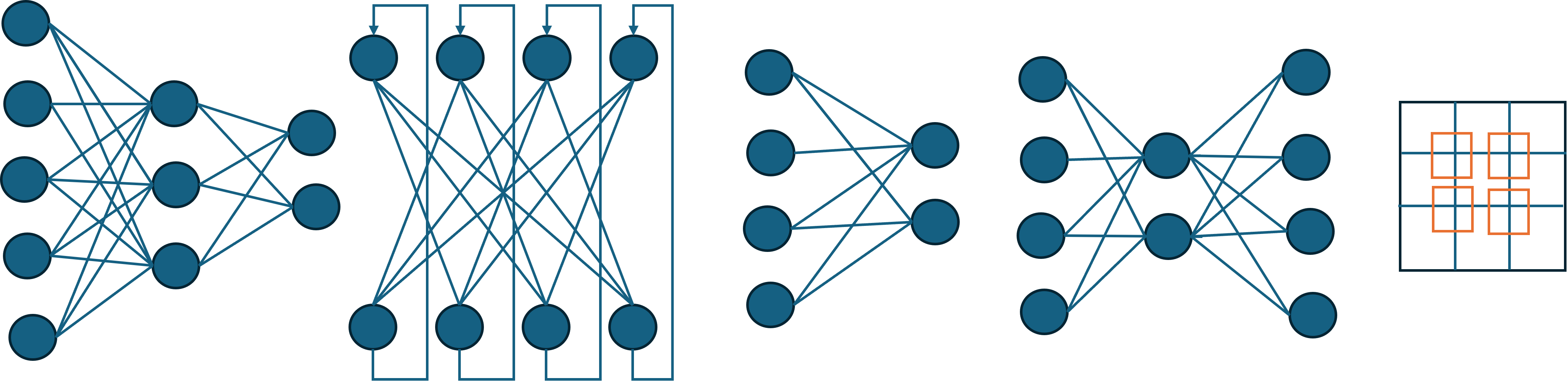
A quantum neural network (QNN) is a mathematical model that combines concepts from quantum computing and artificial neural networks. Neural networks are inspired by biological neurons which have a simple design (e.g. a scalar product followed by an activation function) which is easy to optimize (e.g. using gradient descent) but is very powerful when combined to larger networked structures, so that they can be used as generalized function approximators [35]. Several works have explored these properties by defining parameterized circuits [16] and by modeling components of typical deep models, such as convolutions [9], recurrent neural networks [6] for time-series data, or spiking neurons [43]. The work [7] defines neural networks by modeling each input value and neuron using separate qubits and by defining local unitary functions that activate the neurons while processing the input data. While these approaches have produced valuable results, they differ in important ways from classical neural network processing. For example, the series of unitary matrices used in [7] makes the processing chain non-commutative, which differs from the classical approach of processing neurons independently and in parallel within a layer. Other models require ancilla qubits or repeat-until-success circuits [16]. Figure 2 gives a collage of examples of commonly used realizations of neurons and neural networks.

Figure 2: Examples for existing architectures to represent neurons on a quantum device (taken from [17, 69, 65, 4]).

Motivated by this, we propose an alternative model that is closer to the classical perceptron, easier to interpret and connect, and still powerful enough to map a neural network onto a quantum computer and to optimize it. We therefore represent a neuron using CRX-gates, use layers in the neural network whose operations commute within each layer (as in a shallow neural network), and propose an optimization algorithm that allows us to enforce constraints such as connection cutting and weight sharing. This leads to an efficient realization of classical architectures such as Hopfield networks, restricted Boltzmann Machines, convolutions and more.

III Quantum perceptron with probabilistic activation

Figure 3: Concept of a quantum perceptron with probabilistic activation. The bias is represented as an RX-Gate and the binary input qubits $a_{i}$ increment the probability of neuron excitation by their angular components $\omega_{i}$. To ensure a linear and additive behavior of the angles, directly mapping to the probabilities, the $asin$-function is used. The right image visualizes the qubit activation on the Bloch sphere (just the real part is shown) and the effect of rotating the qubits, based on the bias and controlled RX-gates.

The general idea about modeling the behavior or a perceptron with probabilistic activation on a quantum computer is shown in Figure 3: The (binary) inputs are manipulating the activation probability of the perceptron by using RX-Gates (for the bias) and Controlled RX-Gates. The aim is to use input qubits to increase the probability of the perceptron activation by a value $a_{i}$. To translate this probability score to an appropriate rotation we simply use $asin(\sqrt{a_{i}})$ as angular measure for the rotation. The additive impact is shown in Figure 4: For the first qubit we set as activation probability the value $0.6$ and for the second one the value $0.4$. The combination of all possible states $(00,10,01,11)$ leads to the observation probabilities shown in the histograms below: If no qubit is activated, the probability to measure $0$ is one, the latter qubit raises the score to $0.6$ and if only the front qubit (the upper one) is activated, the probability of the perceptron to be activated is $0.4$. Finally, if both qubits are $1$, the perceptron activates with probability $1.0$.

Figure 4: Example activations for a perceptron with two binary inputs. The weights are set to [0.4 0.6]. The bottom histograms demonstrate the additive increase of the activation probability.

Please note that cumulative values greater than $1$ lead to a decrease of the activation probability. This allows the perceptron to be more expressive than a classical perceptron with e.g. a sigmoid activation. For example, the weights $(\omega_{1}=1,\omega_{2}=1)$ will lead to the implementation of a xor-function:

$$|00\rangle \rightarrow |0\rangle$$

$$|01\rangle \rightarrow |1\rangle$$

$$|10\rangle \rightarrow |1\rangle$$

$$|11\rangle \rightarrow |0\rangle$$ (2)

This can also be motivated from medical findings, as Gidon and colleagues [26] found that there exists a type of pyramidal neuron in the human cerebral cortex that can learn the XOR function. This is impossible with single artificial perceptrons using sigmoidal, ReLU, leaky ReLU, PReLU, GELU, or other (typical) activation functions. As mentioned before, the sin-function is already non-linear and our model shares similarities to networks which use Radial-Basis functions for activation [54]. Please also note that in the digital domain, dropout layers are a common approach to realize probabilistic activations [25], but it also requires repetitive evaluations of the same (large) model to gain a probability distribution of activations.

III.1 Optimization of Quantum Neural Network weights

For optimization of the Quantum Neural Network we use an approach known from stochastic approximation: The Kiefer–Wolfowitz algorithm was introduced in 1952 [39] and was motivated by the Robbins–Monro algorithm [59]. The algorithm has been presented as a method which can stochastically estimate the maximum (or minimum) of a function. Let $M(x)$ be a function which has (wlog) a maximum at the point $\theta$. It is further assumed that $M(x)$ is reasonably smooth. The structure of the algorithm follows a gradient-like method, with the iterates being generated as

$$x_{n+1} = x_{n}+a_{n}\left(\frac{M(x_{n}+c_{n})-M(x_{n}-c_{n})}{2c_{n}}\right)$$

where $M(x_{n}+c_{n})$ and $M(x_{n}-c_{n})$ are independent. Thus, the gradient of $M(x)$ is approximated by a central difference method with a damping factor $a_{n}$ slightly shifting the solution towards an optimum. Our method works in a simulated annealing scheme: Simulated Annealing (SA) is a probabilistic technique to approximating the optimum of a given function [42]. The name derives from annealing in metallurgy where the process involves heating and a controlled cooling of a material to change and control its physical properties. As an optimization scheme the algorithm works iteratively with respect to time $t$ given a state $x_{t}$, similar to the Kiefer-Wolfowitz algorithm. At each step, the simulated annealing heuristic samples a neighboring state $\hat{x}_{t}$ of the current state $x_{t}$, e.g. based on an approximate gradient. Then a probabilistic decision is made to decide whether to move to the new state $x_{t+1}=\hat{x}_{t}$ or to remain in the former state $x_{t+1}=x_{t}$. The probability of making the transition from the current state $x_{t}$ to the new state $\hat{x}_{t}$ is defined by an acceptance probability function $P(e(x_{t}),e(\hat{x}_{t}),T)$. The function $e(x)$ evaluates the energy of this state, which is in our case the fitness score given by the optimization task (e.g. the $\ell_{2}$-loss). The parameter $T$ is a time-dependent variable dictating the behavior of the stochastic process according to a cooling scheme or annealing schedule. The $P$ function is typically chosen in such a way that the probability of accepting an uphill move decreases with time and it decreases as the difference $e(\hat{x}_{t})-e(x_{t})$ increases. Thus, in contrast to a strict gradient descent, a small increase in error is likely to be accepted so that local minima can be avoided over the iterations, whereas a larger error increase is not likely to be accepted. A typical function for $P$ takes the form

$$P(e(x_{t}),e(\hat{x}_{t}),T)\propto\exp\left(-\frac{e(\hat{x}_{t})-e(x_{t})}{kT}\right),$$ (3)

with $k$ a damping factor $k>0$. Thus, our optimization is based on a local stochastic search scheme which is not strict gradient descent. Please note that several neural networks have special requirements on the networks, such as shared weights or symmetry properties. Using stochastic search, as proposed here, can ensure certain constraints during optimization.

IV Models and Experiments

IV.1 Shallow Neural Networks

Figure 5: Implementation of a shallow neural network on a quantum device. This model consists of 4 qubits as input, three hidden neurons and two output neurons. The (C)RX-Gates contain the learnable parameters.

A shallow neural network is typically a neural network that consists of only one hidden layer between the input and output layers [10, 11]. The general structure is to connect all input elements to each perceptron of the hidden layer which is then called a fully connected layer. Afterwards the hidden perceptrons are connected to the output layer. Figure 5 demonstrates the implementation of a shallow neural network on a quantum device based on our earlier defined stochastic perceptrons. The shown model consists of 4 qubits as input which are connected to three hidden neurons by using CRX-Gates. The hidden neurons are three additional qubits. The RX-Gate itself is the bias. Afterwards, the three qubits representing the neural activity are connected to two qubits acting as output neurons. The (C)RX-Gates contain with the rotation angles $\omega_{i}$ the learnable parameters.

Figure 6: TSNE-Plots of the used UCI datasets for classification, the iris dataset (left), the wine dataset (middle) and the zoo dataset (right).

Figure 7: Convergence of the optimization algorithm during training the iris dataset. Shown is the loss decrease in blue and the accuracy (of the test data) in red. In this run, the algorithm could perfectly classify all test samples.

We used the optimization procedure summarized in Section III.1 and for the experiments, the classical iris, wine and zoo datasets were used. The datasets present multi-class classification tasks, with three categories for the iris and wine datasets and seven categories for the zoo dataset. The datasets are all available at the UCI repository [22]. Additionally, we performed experiments on a subset of the well-known MNIST dataset [19] for digit classification. Here, we restricted the model to five classes (the digits $0\ldots 4$) and used 4500 (random) samples for training and 500 for testing.

To model a classification task using a quantum circuit, first the data is encoded as a higher-dimensional binary vector. Taking the iris dataset as a toy example, it consists of $4$ dimensional data encoding sepal length, sepal width, petal length and petal width. After separating training and test data, a kMeans clustering on each dimension with $k=3$ is used on the training data. Thus, every datapoint can be encoded in a $4\times 3=12-$dimensional binary vector which contains exactly $4$ non-zero entries. For the given cluster centers, the same can be done with the test data. Thus, a binary encoding is used to represent the datasets. Please note that binarized neural networks (BNNs), which are neural networks with weights and activations in $(-1,1)$, can achieve comparable test performance to standard neural networks, but allow for highly efficient implementations on resource limited systems [33].

Figure 7 shows the convergence behavior of the optimization algorithm during training the iris dataset. The loss decrease over iterations is shown in blue and the accuracy (of the test data) in red. In this run, the algorithm could perfectly classify all test samples.

Dataset Perc. qubits Classes Acc Acc (gd) ours Iris 4 20 3 84 $\%$ 95 $\%$ ($\pm$ 21) ($\pm$ 5) Zoo 5 18 7 72 $\%$ 87 $\%$ ($\pm 22$) ($\pm 5$) wine 3 18 3 75 $\%$ 95 $\%$ ($\pm 5$) ($\pm 4$) mnist₅ 8 38 5 75 $\%$ 99 $\%$ ($\pm 28$) ($\pm 5$)

Table 1: Test datasets overview and performance. The column gd indicates the performance when using a plain vanilla gradient descent approach for optimization. Please note the high variance of the results, due to local minima.

Table 1 summarizes the four example datasets and the overall performance. It contains the used qubits to represent the problem as quantum code, the amount of target classes and the achieved accuracy with gradient descent using autodiff (gd) and our optimized quantum circuits (ours). Please note the large variance of gradient descent, which results in a low average score due to local minima during optimization. Thus, when starting from a random seed, the optimizer often converges to good results comparable to our approach, but frequently the optimization fails completely. This effect of getting stuck in local minima is well known and documented in the machine learning literature [55]. For this experiment, we did not perform data augmentation, dropout or other common methods to increase performance of gradient descent. The combination of gradient descent with common measures to improve performance leads to similar results as our model.

IV.2 Hopfield Networks

Introduced in 1982 [32], a Hopfield network consists of a one-layer recurrent network with the input dimension being equal to the output dimension. Its main purpose is to act as autoassociative memory, e.g. for a given sample, the memory should retrieve a piece of memorized data. Hopfield networks can be applied in de-noising or removing interference from an input or they can be used to determine whether the given input is known or unknown. Although Hopfield networks are a well-established topology, they have received renewed attention recently [57].

Figure 8: Hopfield Network and its corresponding Quantum Circuit for four input qubits. The red boxes are visual marks to show that an input neuron has no direct connection to its corresponding output neuron.

Figure 9: Pattern retrieval of a 9-dimensional input data. The patterns in the upper left (red box) are to be memorized from the Hopfield network. The first row shows the test pattern and the second row the retrieval pattern (after one iteration). Whereas the memorized patterns are successfully reconstructed, the noisy input patterns have activation probabilities leading to the closest memorized pattern.

Figure 10: Pattern retrieval of disturbed input data (left). As recurrent model, the optimized Hopfield network can recover the memorized pattern within a few model iterations (right).

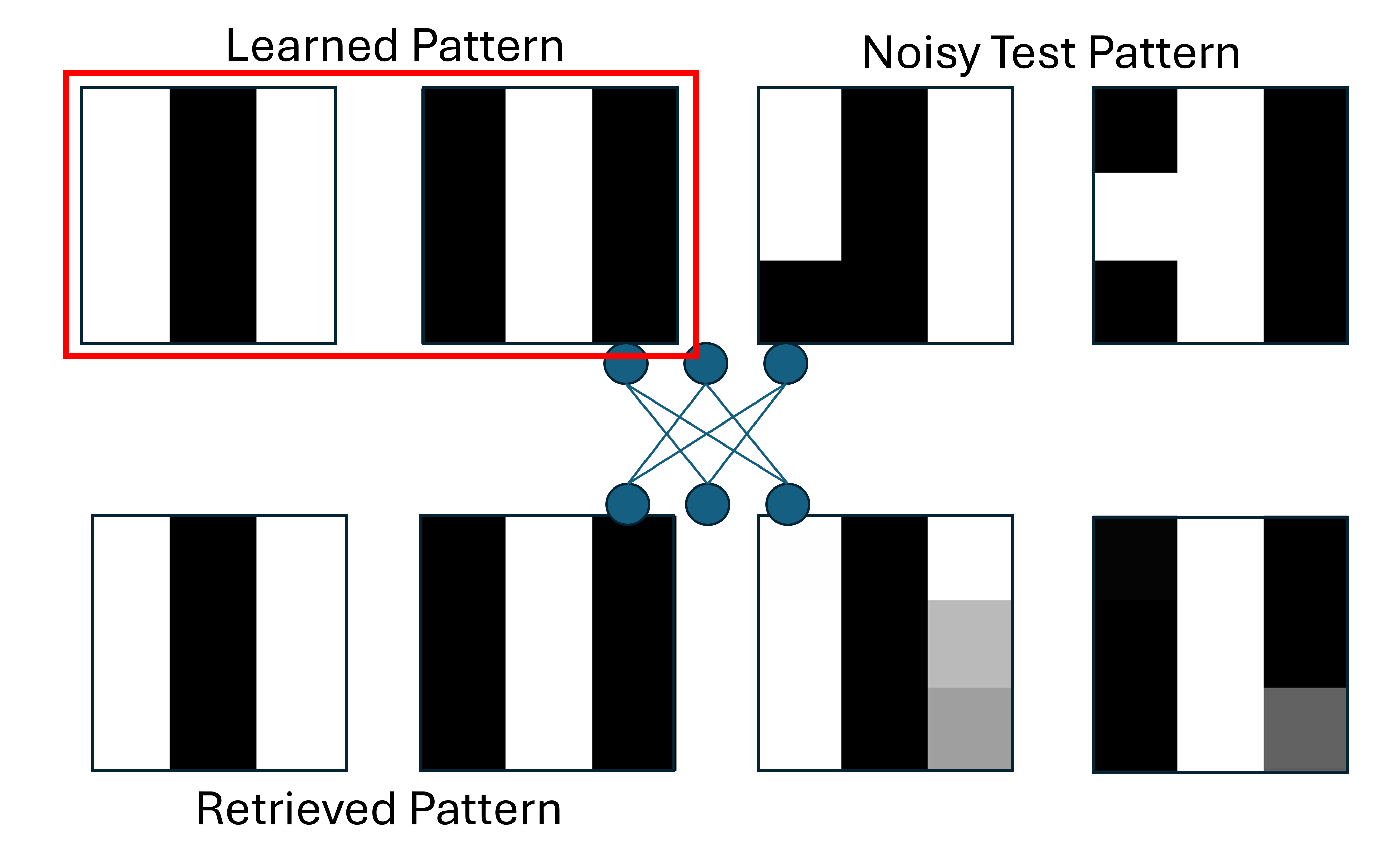
The units in Hopfield nets are binary threshold units $\in\{0,1\}$, the interactions $\omega_{i,j}$ between neurons are defined to be symmetric ($\omega_{i,j}=\omega_{j,i}$) and no unit has a connection with itself ($\omega_{i,i}=0$). The classical form of a Hopfield network is shown on the left of Figure 8. The corresponding expression as quantum code is depicted on the right; the red squares mark that there is no connection from an input dimension to its output dimension. Thus, the remaining neurons have to determine the activation of a certain input value. Hopfield networks are recurrent, which means that the output is fed back as input and the process is iterated until convergence to a memorized pattern. Figure 9 summarizes an experiment for memorizing and retrieving patterns. The goal is to learn two patterns (of vertical stripes) of a 9-dimensional ($3\times 3$) input data. They are depicted in the red box at the upper left. After optimization of the model we can use it for inference. The first row in Figure 9 shows the test pattern and the second row the retrieval pattern (after one iteration). Whereas the memorized patterns are successfully reconstructed, the noisy input patterns have activation probabilities leading to the closest memorized pattern.

Figure 10 shows the evolution towards a memorized pattern over several iterations of the recurrent model during the quantum simulations.

IV.3 Restricted Boltzmann Machines

Figure 11: RBM Network and its corresponding Quantum Circuit for four input qubits and two latent space neurons. The red connections indicate a weight sharing. The RBM is bidirectional, thus the weights are used for both, encoding and decoding.

Some decades after the introduction of the perceptron, around 1985, the Boltzmann Machine (BM) was invented [2]. It is a network of symmetrically connected, neuron-like binary units. Learning the weights of such a connectionist system allows the Boltzmann Machine to discover features that represent complex properties in training data. A modification is a so-called Restricted Boltzmann Machine (RBM) which consists of a two layer architecture with one layer of visible units and one layer of hidden units. RBMs were initially invented under the name Harmonium by Paul Smolensky in 1986 [67]. An RBM can be interpreted as a bipartite graph with symmetric connections, see Figure 11.

Figure 12: Example features from the Iris dataset and its encoding and decoding. Since the RBM is a probabilistic model, the gray values indicate the probability for a perceptron activation. Thus, already two hidden perceptrons are sufficient to represent the 12-dimensional input space with reasonable quality.

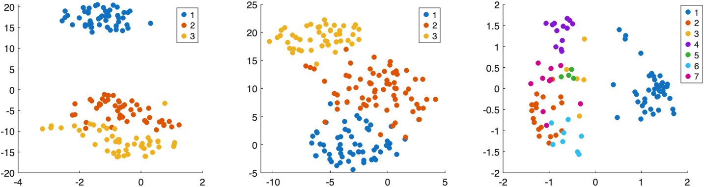
Such a model can be useful for dimensionality reduction, classification, regression, collaborative filtering, feature learning and topic modeling. Indeed, Restricted Boltzmann Machines received increasing attention during and after the $1 million Netflix challenge [63]. In contrast to deterministic models, RBMs are generative stochastic networks, where the neuron activation is probabilistic. Thus, RBMs have binary units which turn on/off according to probabilities determined by the weights, which is a model fitting perfectly to our quantum formulation. The units in Restricted Boltzmann Machines are binary threshold units $\in[0,1]$, the interactions $\omega_{i,j}$ between neurons are defined to be symmetric. The weights need to be suited for the projection onto the hidden space and vice versa the reconstruction from the hidden space to the input space. Thus, for an unsupervised learning task, the RBM can be unrolled to an autoencoder like architecture with shared weights among the encoder and decoder, indicated by the dashed connections in Figure 11. This has also been pointed out by [67]. Similar to the Hopfield architecture, the shared weights decrease the complexity of the stochastic optimization procedure we described beforehand, as the amount of variables is effectively decreasing. As a simple example, we use the iris dataset with a binary representation of dimension 12, so 12 qubits are used as input values. We then optimize for a two dimensional latent space and uplift the representation to 12 dimensions again, as visualized in Figure 11 (just using 12 instead of four input qubits shown in the image). Figure 12 shows on the right the reconstruction quality of (unseen) data samples after optimizing the model. As can be seen, even though there is a heavy compression enforced (to two dimensions), the reconstruction is of reasonable quality.

IV.4 Autoencoder

An autoencoder is a neural network which is commonly used to learn efficient representations from data [30]. It consists of two parts, an encoder branch and a decoder branch with a bottleneck layer in the middle. The aim of the model is to solve a copying task by replicating the input signal at the output. Due to the bottleneck layer, which has usually less dimensions than the input data, the model has to learn a compressed representation of the training data [5]. Autoencoders have been modified to variational autoencoders [40], sparse autoencoders [34], vector quantized autoencoders [58] and more in the past. Still, an autoencoder is a common approach for data compression, subspace projection and data analysis. The implementation of a quantum circuit to realize an autoencoder is very similar to the circuit shown in Figure 11. The only difference is that weight sharing is removed, which means that there are more parameters to optimize (which in return can take longer during training), but the separated weights for encoding and decoding allow for a higher capacity for representing data. We performed a similar experiment on the Iris dataset used in the RBM framework for the autoencoder. Again, a 12 dimensional input vector is reduced to two dimensions and reconstructed back to 12 dimensions. The outcome of the reconstruction is shown in Figure 13. It can be seen that the reconstruction quality improved over an RBM, shown in Figure 12. This expected result comes from the dropped weight sharing which allows the model to separate information for encoding and decoding. This leads to a higher capacity of the neural network.

Figure 13: Example features from the Iris dataset and its encoding and decoding using an autoencoder. Since the autoencoder can carry more information than an RBM, the overall reconstruction quality is higher, compared to the former model.

IV.5 Convolutional neural network

Figure 14: Convolutional neural network

A convolutional neural network (CNN) is a feedforward neural network that learns features by optimizing for linear shift-invariant filters [44]. A core concept is a so-called weight sharing and connection cutting which leads to a linear form of a Toeplitz matrix to be optimized [15].

Figure 15: The Bars and Stripes patterns.

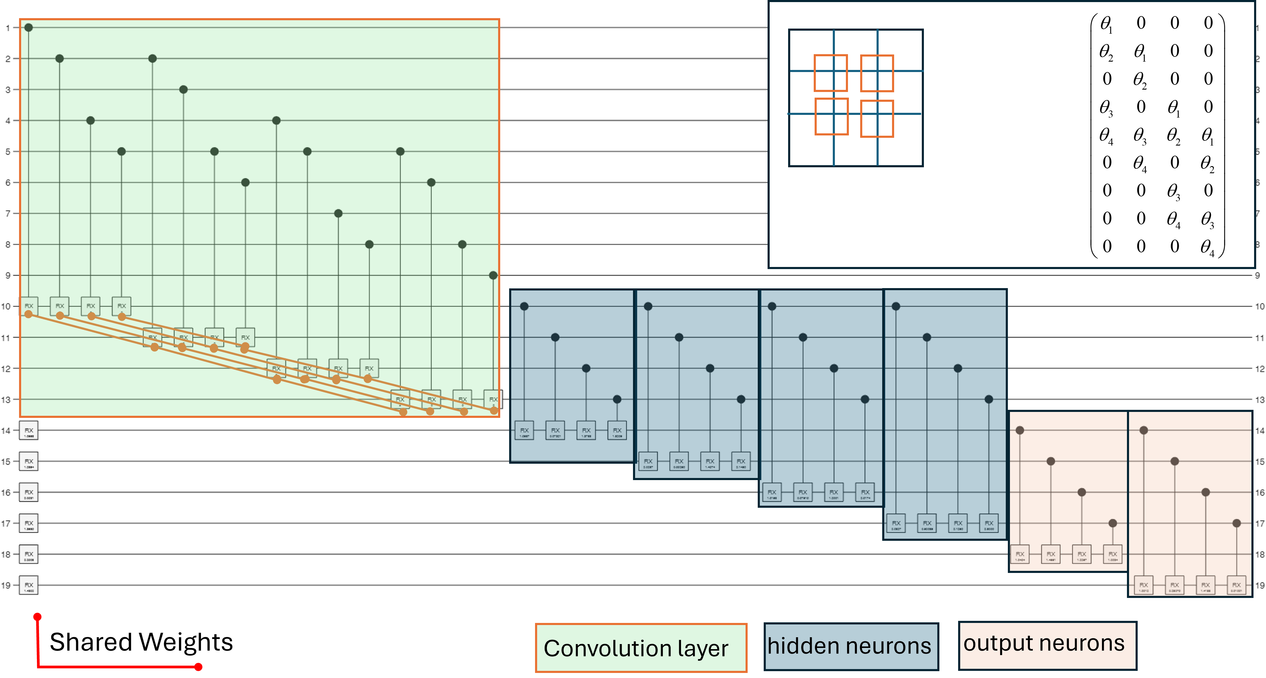
This type of deep learning network has been applied to many different types of data including text, images and audio [20, 45]. It can be seen as the de facto standard in deep learning-based computer vision and has only recently been replaced by alternative architectures such as the transformer [46]. The concept of a convolution is visualized in the upper right corner in Figure 14. A $2\times 2$ kernel is placed over an image patch, the image values are multiplied with the kernel weights and summed up. The kernel is then shifted to the next patch and processed with the same weights. Thus, it is a linear shift-invariant operation which can be expressed as a fully connected layer with several connections being dropped and the weights being arranged as a Toeplitz matrix. This again leads to a high reduction of optimization variables which makes the optimization simpler, compared to several fully connected layers. Thus, overfitting is easier prevented and it is possible to learn concepts for classification in an easier way. Figure 14 shows the quantum code of a convolutional neural network with one convolution layer in the beginning and then a fully connected layer before continuing to the output layer. We used this model to train simple pattern classification tasks, such as bars and stripes, see Figure 15: The input is a $3\times 3$ patch and the task is to classify if the input pattern belongs to the bars and stripes examples, or not. After optimizing the model, the network can perfectly classify and differentiate the examples. Please note that the task is quite imbalanced, as there are only $8$ positive patterns and $2^{9}-8$ negative patterns. Still, the model can solve this task after optimization. Due to the probabilistic activations, the average accuracy varies between $99\%$ and $100\%$.

IV.6 Generative neural network

Figure 16: Binary neural network for classifying a simple pattern

Figure 17: Architecture of the Grover circuit for generating patterns.

Figure 18: Sampled bins when executing Grovers algorithm

Figure 19: Histogram after executing Grovers algorithm for a neural network which detects patterns with two dots.

Generative AI (GenAI) is an increasingly important field of research and comprises the challenge to use data to generate new results or contents such as texts, speech, audio recordings, images or videos. Early works date back to 2002 [53, 12] with the real breakthrough in using generative adversarial networks [27, 68], also called GANs, vector quantized variational autoencoders [72], denoted as VQ-VAEs and the so-called diffusion models [18, 60]. The core idea of a GAN is to train two neural networks which compete in a min-max game, where one model, the so-called generator, tries to fool the other model, called the discriminator. Whereas the discriminator has to distinguish real data from generated data, the generator takes a random pattern as input to generate an artificial sample. Typical challenges for GANs are the unstable training behavior and mode collapse. This led to alternative approaches, such as diffusion models. A diffusion model has two main parts, first the forward diffusion process, and secondly the reverse sampling process. The goal of a diffusion model is to learn a diffusion process such that generated elements are distributed in accordance with an original dataset. In practice, e.g. for image generation, the diffusion model is trained in such a way to reverse the process of adding noise to an image. Thus, when starting with an image composed of random noise, the network is applied iteratively to denoise the image, leading to novel examples. We do not go into details on the vast amount of literature, instead we refer to recent surveys, such as [28, 64, 66]. All approaches are characterized by involving a stochastic process, either for a denoising of a random pattern (in diffusion frameworks), or for a min-max game to fool a discriminator, e.g. when using a GAN.

In the last years, the Grover algorithm [29] has gained increased attention in quantum computing as it is a celebrated quantum algorithm that provides a provable quadratic speedup over classical algorithms for searching in an unsorted database. Especially for quantum annealing [47, 3] and quantum machine learning [37, 1, 38], the Grover algorithm is a very classical tool to use.

The core idea for a quantum GenAI circuit is to use our quantum neural networks (e.g. for classification of patterns) to combine it with a Grover search, such that examples can be sampled which fulfill a classification property. Figure 16 shows the architecture of our quantum neural network to classify a simple binary pattern. Here the goal is to classify if there is exactly one dot in the pattern or not. After training the model we keep the circuit frozen and generate the circuit and its reverse to get the so-called oracle, see Figure 17. Now we generate a circuit by first bringing the input qubits into superposition. Then the oracle is applied and afterwards a diffusion circuit follows. Now, we can execute the circuit and visualize the probabilities for sampling specific patterns. A resulting example distribution is shown in Figure 18. Thus, as expected, the classified patterns are sampled with a much higher likelihood than the remaining patterns. Figure 19 shows the result for a neural network which can detect two bit patterns. Instead of a simple $2\times 2$ pattern, imagine a frozen quantum network which can classify whether an image depicts a human face or not. In combination with superposition in front and the Grover circuit afterwards, the sampled proposals are more likely to be classified as a face. Thus, sampling this circuit leads to a highly-efficient generative model.

V Conclusion

In this work we presented a formulation to express and optimize stochastic neural networks as quantum circuits for gate-based quantum computing. Our work is inspired by a classical perceptron and we use CRX-Gates to drive the stochastic activation of a neuron. A combination of several such stochastically activating neurons are used to express a quantum neural network. The Kiefer-Wolfowitz algorithm in combination with simulated annealing is used for training the network weights. It has the advantage that it can easily respect constraint on the weights, such as shared weights, connection cutting and more. This allows in a very intuitive way to optimize several topologies and models. Our experiments present shallow fully connected networks, Hopfield Networks, Restricted Boltzmann Machines, Autoencoders and convolutional neural networks. We finally demonstrate the combination of our optimized neural networks as an oracle within the Grover algorithm to present a circuit that allows for a quantum-driven generative AI.

Funding Declaration

This work was supported, in part, by the Federal Ministry of Research, Technology and Space (BMFTR), Germany under the AI service center KISSKI (grant no. 01IS22093C), the QC service center QUICS (grant no. 13N17418), by the Quantum Valley Lower Saxony and by Germany’s Excellence Strategies EXC-2122 PhoenixD and EXC-2123 Quantum Frontiers.

References

- [1] Muhammad AbuGhanem. Characterizing grover search algorithm on large-scale superconducting quantum computers. Scientific Reports, 15(1):1281, Jan 2025.
- [2] David H. Ackley, Geoffrey E. Hinton, and Terrence J. Sejnowski. A learning algorithm for boltzmann machines. Cogn. Sci., 9:147–169, 1985.
- [3] B. Apolloni, C. Carvalho, and D. de Falco. Quantum stochastic optimization. Stochastic Processes and their Applications, 33(2):233–244, 1989.
- [4] Qi Bai and Xianliang Hu. Quantity study on a novel quantum neural network with alternately controlled gates for binary image classification. Quantum Information Processing, 22(5):184, Apr 2023.
- [5] Dor Bank, Noam Koenigstein, and Raja Giryes. Autoencoders, pages 353–374. Springer International Publishing, Cham, 2023.
- [6] Johannes Bausch. Recurrent quantum neural networks. In Proceedings of the 34th International Conference on Neural Information Processing Systems, NIPS ’20, Red Hook, NY, USA, 2020. Curran Associates Inc.
- [7] Kerstin Beer, Dmytro Bondarenko, Terry Farrelly, Tobias J. Osborne, Robert Salzmann, Daniel Scheiermann, and Ramona Wolf. Training deep quantum neural networks. Nature Communications, 11(1):808, Feb 2020.
- [8] Yoshua Bengio, Aaron Courville, and Pascal Vincent. Representation learning: A review and new perspectives. IEEE Transactions on Pattern Analysis and Machine Intelligence, 35(8):1798–1828, 2013.
- [9] Pablo Bermejo, Paolo Braccia, Manuel S. Rudolph, Zoë Holmes, Lukasz Cincio, and M. Cerezo. Quantum convolutional neural networks are (effectively) classically simulable, 2024.
- [10] C. M. Bishop. Pattern Recognition and Machine Learning (Information Science and Statistics). Springer-Verlag New York, Inc., Secaucus, NJ, USA, 2006.
- [11] Christopher Michael Bishop and Hugh Bishop. Deep Learning - Foundations and Concepts. 1 edition, 2023.
- [12] David M. Blei, Andrew Y. Ng, and Michael I. Jordan. Latent dirichlet allocation. J. Mach. Learn. Res., 3(null):993–1022, March 2003.
- [13] Nick Brown. Exploring the versal ai engines for accelerating stencil-based atmospheric advection simulation. In Proceedings of the 2023 ACM/SIGDA International Symposium on Field Programmable Gate Arrays, FPGA ’23, page 91–97, New York, NY, USA, 2023. Association for Computing Machinery.
- [14] Tom B. Brown, Benjamin Mann, Nick Ryder, Melanie Subbiah, Jared Kaplan, Prafulla Dhariwal, Arvind Neelakantan, Pranav Shyam, Girish Sastry, Amanda Askell, Sandhini Agarwal, Ariel Herbert-Voss, Gretchen Krueger, Tom Henighan, Rewon Child, Aditya Ramesh, Daniel M. Ziegler, Jeffrey Wu, Clemens Winter, Christopher Hesse, Mark Chen, Eric Sigler, Mateusz Litwin, Scott Gray, Benjamin Chess, Jack Clark, Christopher Berner, Sam McCandlish, Alec Radford, Ilya Sutskever, and Dario Amodei. Language models are few-shot learners. In Proceedings of the 34th International Conference on Neural Information Processing Systems, NIPS ’20, Red Hook, NY, USA, 2020. Curran Associates Inc.
- [15] Albrecht Böttcher and Sergei Grudsky. Toeplitz Matrices, Asymptotic Linear Algebra, and Functional Analysis. 01 2000.
- [16] Yudong Cao, Gian Giacomo Guerreschi, and Alán Aspuru-Guzik. Quantum neuron: an elementary building block for machine learning on quantum computers, 2017.
- [17] Iris Cong, Soonwon Choi, and Mikhail D. Lukin. Quantum convolutional neural networks. Nature Physics, 15(12):1273–1278, Dec 2019.
- [18] Florinel-Alin Croitoru, Vlad Hondru, Radu Tudor Ionescu, and Mubarak Shah. Diffusion models in vision: A survey. IEEE Transactions on Pattern Analysis and Machine Intelligence, 45(9):10850–10869, 2023.
- [19] Li Deng. The mnist database of handwritten digit images for machine learning research. IEEE Signal Processing Magazine, 29(6):141–142, 2012.
- [20] Tiancan Deng. A survey of convolutional neural networks for image classification: Models and datasets. In 2022 International Conference on Big Data, Information and Computer Network (BDICN), pages 746–749, 2022.
- [21] Carl Doersch and Andrew Zisserman. Multi-task self-supervised visual learning. In 2017 IEEE International Conference on Computer Vision (ICCV), pages 2070–2079, 2017.
- [22] Dheeru Dua and Casey Graff. UCI machine learning repository. http://archive.ics.uci.edu/ml, 2017.
- [23] Sourav Dutta, Georgios Detorakis, Abhishek Khanna, Benjamin Grisafe, Emre Neftci, and Suman Datta. Neural sampling machine with stochastic synapse allows brain-like learning and inference. Nature Communications, 13(1):2571, May 2022.
- [24] M. Ehsan Abbasnejad, Anthony Dick, and Anton van den Hengel. Infinite variational autoencoder for semi-supervised learning. In Proceedings of the IEEE Conference on Computer Vision and Pattern Recognition (CVPR), July 2017.
- [25] Yarin Gal and Zoubin Ghahramani. Dropout as a bayesian approximation: Representing model uncertainty in deep learning. In Maria Florina Balcan and Kilian Q. Weinberger, editors, Proceedings of The 33rd International Conference on Machine Learning, volume 48 of Proceedings of Machine Learning Research, pages 1050–1059, New York, New York, USA, 20–22 Jun 2016. PMLR.
- [26] Albert Gidon, Timothy Adam Zolnik, Pawel Fidzinski, Felix Bolduan, Athanasia Papoutsi, Panayiota Poirazi, Martin Holtkamp, Imre Vida, and Matthew Evan Larkum. Dendritic action potentials and computation in human layer 2/3 cortical neurons. Science, 367(6473):83–87, 2020.
- [27] Ian J. Goodfellow, Jean Pouget-Abadie, Mehdi Mirza, Bing Xu, David Warde-Farley, Sherjil Ozair, Aaron Courville, and Yoshua Bengio. Generative adversarial nets. In Z. Ghahramani, M. Welling, C. Cortes, N. Lawrence, and K.Q. Weinberger, editors, Advances in Neural Information Processing Systems, volume 27. Curran Associates, Inc., 2014.
- [28] Roberto Gozalo-Brizuela and Eduardo C. Garrido-Merchán. A survey of generative ai applications, 2023.
- [29] Lov K. Grover. From schrödinger’s equation to the quantum search algorithm. American Journal of Physics, 69(7):769–777, 07 2001.
- [30] G. E. Hinton and R. R. Salakhutdinov. Reducing the dimensionality of data with neural networks. Science, 313(5786):504–507, 2006.
- [31] Noah Hollmann, Samuel Müller, Lennart Purucker, Arjun Krishnakumar, Max Körfer, Shi Bin Hoo, Robin Tibor Schirrmeister, and Frank Hutter. Accurate predictions on small data with a tabular foundation model. Nature, 637(8045):319–326, Jan 2025.
- [32] J J Hopfield. Neural networks and physical systems with emergent collective computational abilities. Proceedings of the National Academy of Sciences, 79(8):2554–2558, 1982.
- [33] I. Hubara, M. Courbariaux, D. Soudry, R. El-Yaniv, and Y. Bengio. Binarized neural networks. In Advances in Neural Information Processing Systems, volume 29. Curran Associates, Inc., 2016.
- [34] Robert Huben, Hoagy Cunningham, Logan Riggs Smith, Aidan Ewart, and Lee Sharkey. Sparse autoencoders find highly interpretable features in language models. In The Twelfth International Conference on Learning Representations, 2024.
- [35] Subhash C. Kak. Quantum neural computing. volume 94 of Advances in Imaging and Electron Physics, pages 259–313. Elsevier, 1995.
- [36] Phillip Kaye, Raymond Laflamme, and Michele Mosca. An Introduction to Quantum Computing. Oxford University Press, Inc., USA, 2007.
- [37] Bikram Khanal, Javier Orduz, Pablo Rivas, and Erich Baker. Supercomputing leverages quantum machine learning and grover’s algorithm. J. Supercomput., 79(6):6918–6940, November 2022.
- [38] Bikram Khanal, Pablo Rivas, Javier Orduz, and Alibek Zhakubayev. Quantum machine learning: A case study of grover’s algorithm. In 2021 International Conference on Computational Science and Computational Intelligence (CSCI), pages 79–84, 2021.
- [39] J. Kiefer and J. Wolfowitz. Stochastic Estimation of the Maximum of a Regression Function. The Annals of Mathematical Statistics, 23(3):462 – 466, 1952.
- [40] Diederik P Kingma and Max Welling. Auto-encoding variational bayes, 2022.
- [41] Alexander Kirillov, Eric Mintun, Nikhila Ravi, Hanzi Mao, Chloe Rolland, Laura Gustafson, Tete Xiao, Spencer Whitehead, Alexander C. Berg, Wan-Yen Lo, Piotr Dollar, and Ross Girshick. Segment anything. In Proceedings of the IEEE/CVF International Conference on Computer Vision (ICCV), pages 4015–4026, October 2023.
- [42] S. Kirkpatrick, C. D. Gelatt, and M. P. Vecchi. Optimization by simulated annealing. Science, 220(4598):671–680, 1983.
- [43] Lasse Bjørn Kristensen, Matthias Degroote, Peter Wittek, Alán Aspuru-Guzik, and Nikolaj T. Zinner. An artificial spiking quantum neuron. npj Quantum Information, 7(1):59, Apr 2021.
- [44] Yann LeCun, Yoshua Bengio, and Geoffrey Hinton. Deep learning. Nature, 521(7553):436–444, May 2015.
- [45] Zewen Li, Fan Liu, Wenjie Yang, Shouheng Peng, and Jun Zhou. A survey of convolutional neural networks: Analysis, applications, and prospects. IEEE Transactions on Neural Networks and Learning Systems, 33(12):6999–7019, 2022.
- [46] Tianyang Lin, Yuxin Wang, Xiangyang Liu, and Xipeng Qiu. A survey of transformers. AI Open, 3:111–132, 2022.
- [47] Andrew Lucas. Ising formulations of many np problems. Frontiers in Physics, Volume 2 - 2014, 2014.
- [48] Junwei Ma, Valentin Thomas, Rasa Hosseinzadeh, Hamidreza Kamkari, Alex Labach, Jesse C Cresswell, Keyvan Golestan, Guangwei Yu, Anthony L Caterini, and Maksims Volkovs. Tabdpt: Scaling tabular foundation models on real data. arXiv preprint arXiv:2410.18164, 2024.
- [49] Gengchen Mai, Weiming Huang, Jin Sun, Suhang Song, Deepak Mishra, Ninghao Liu, Song Gao, Tianming Liu, Gao Cong, Yingjie Hu, Chris Cundy, Ziyuan Li, Rui Zhu, and Ni Lao. On the opportunities and challenges of foundation models for geoai (vision paper). ACM Trans. Spatial Algorithms Syst., 10(2), July 2024.
- [50] Christopher D. Manning. Human language understanding & reasoning. Daedalus, 151(2):127–138, 05 2022.
- [51] W. McCulloch and W. Pitts. A logical calculus of ideas immanent in nervous activity. Bulletin of Mathematical Biophysics, 5:127–147, 1943.
- [52] Berndt Müller, Joachim Reinhardt, and Michael T. Strickland. Stochastic Neurons, pages 38–45. Springer Berlin Heidelberg, Berlin, Heidelberg, 1995.
- [53] Andrew Ng and Michael Jordan. On discriminative vs. generative classifiers: A comparison of logistic regression and naive bayes. In T. Dietterich, S. Becker, and Z. Ghahramani, editors, Advances in Neural Information Processing Systems, volume 14. MIT Press, 2001.
- [54] J. Park and I. W. Sandberg. Universal approximation using radial-basis-function networks. Neural Computation, 3(2):246–257, 06 1991.
- [55] David Picard. Torch.manual seed(3407) is all you need: On the influence of random seeds in deep learning architectures for computer vision, 2023.
- [56] Chao Qian, Xiao Lin, Xiaobin Lin, Jian Xu, Yang Sun, Erping Li, Baile Zhang, and Hongsheng Chen. Performing optical logic operations by a diffractive neural network. Light: Science & Applications, 9(1):59, Apr 2020.
- [57] Hubert Ramsauer, Bernhard Schäfl, Johannes Lehner, Philipp Seidl, Michael Widrich, Thomas Adler, Lukas Gruber, Markus Holzleitner, Milena Pavlović, Geir Kjetil Sandve, Victor Greiff, David Kreil, Michael Kopp, Günter Klambauer, Johannes Brandstetter, and Sepp Hochreiter. Hopfield networks is all you need. arXiv, 2008.02217, 2021.
- [58] Ali Razavi, Aäron van den Oord, and Oriol Vinyals. Generating diverse high-fidelity images with VQ-VAE-2. Curran Associates Inc., Red Hook, NY, USA, 2019.
- [59] Herbert Robbins and Sutton Monro. A stochastic approximation method. The Annals of Mathematical Statistics, 22(3):400–407, 1951.
- [60] Robin Rombach, Andreas Blattmann, Dominik Lorenz, Patrick Esser, and Björn Ommer. High-resolution image synthesis with latent diffusion models. In Proceedings of the IEEE/CVF Conference on Computer Vision and Pattern Recognition, pages 10684–10695, 2022.
- [61] F. Rosenblatt. The perceptron: A probabilistic model for information storage and organization in the brain. Psychological Review, 65(6):386–408, 1958.
- [62] Marco Rudolph, Bastian Wandt, and Bodo Rosenhahn. Same Same But DifferNet: Semi-Supervised Defect Detection with Normalizing Flows . In 2021 IEEE Winter Conference on Applications of Computer Vision (WACV), pages 1906–1915, Los Alamitos, CA, USA, January 2021. IEEE Computer Society.
- [63] Ruslan Salakhutdinov, Andriy Mnih, and Geoffrey Hinton. Restricted boltzmann machines for collaborative filtering. In Proceedings of the 24th International Conference on Machine Learning, ICML ’07, page 791–798, New York, NY, USA, 2007. Association for Computing Machinery.
- [64] Johannes Schneider. Explainable generative ai (genxai): a survey, conceptualization, and research agenda. Artificial Intelligence Review, 57(11):289, Sep 2024.
- [65] Maria Schuld, Ilya Sinayskiy, and Francesco Petruccione. Simulating a perceptron on a quantum computer. Physics Letters A, 379(7):660–663, 2015.
- [66] Sandeep Singh Sengar, Affan Bin Hasan, Sanjay Kumar, and Fiona Carroll. Generative artificial intelligence: a systematic review and applications. Multimedia Tools and Applications, 84(21):23661–23700, Jun 2025.
- [67] P. Smolensky. chapter 6: Information processing in dynamical systems: Foundations of harmony theory. Cogn. Sci.Parallel Distributed Processing, 1:194–281, 1986.
- [68] Yang Song, Rui Shu, Nate Kushman, and Stefano Ermon. Constructing unrestricted adversarial examples with generative models. In S. Bengio, H. Wallach, H. Larochelle, K. Grauman, N. Cesa-Bianchi, and R. Garnett, editors, Advances in Neural Information Processing Systems, volume 31. Curran Associates, Inc., 2018.
- [69] Francesco Tacchino, Chiara Macchiavello, Dario Gerace, and Daniele Bajoni. An artificial neuron implemented on an actual quantum processor. npj Quantum Information, 5(1):26, Mar 2019.
- [70] Michael Tschannen, Olivier Bachem, and Mario Lucic. Recent advances in autoencoder-based representation learning. In Third workshop on Bayesian Deep Learning (NeurIPS 2018), 2018.
- [71] C. Turchetti. Stochastic Models of Neural Networks. IOS Press, NLD, 2004.
- [72] Aaron van den Oord, Oriol Vinyals, and Koray Kavukcuoglu. Neural discrete representation learning. In Proceedings of the 31st International Conference on Neural Information Processing Systems, NIPS’17, page 6309–6318, Red Hook, NY, USA, 2017. Curran Associates Inc.
- [73] Martijn van Otterlo and Marco Wiering. Reinforcement Learning and Markov Decision Processes, pages 3–42. Springer Berlin Heidelberg, Berlin, Heidelberg, 2012.
- [74] Ashish Vaswani, Noam Shazeer, Niki Parmar, Jakob Uszkoreit, Llion Jones, Aidan N. Gomez, Łukasz Kaiser, and Illia Polosukhin. Attention is all you need. In Proceedings of the 31st International Conference on Neural Information Processing Systems, NIPS’17, page 6000–6010, Red Hook, NY, USA, 2017. Curran Associates Inc.
- [75] Jingyi Zhang, Jiaxing Huang, Sheng Jin, and Shijian Lu. Vision-language models for vision tasks: A survey. IEEE Transactions on Pattern Analysis and Machine Intelligence, 46(8):5625–5644, 2024.