Reevaluating Thermal Instability in a Uniform Plasma: An Extended Analysis of Instability Domains

Abstract

Thermal instability plays a crucial role in the dynamics of astrophysical plasmas. Building upon the foundational work of Field (1965) and the subsequent analysis by Waters and Proga (2019), this study revisits thermal instability in a uniform, non-magnetic medium. We aim to reevaluate and expand the understanding of instability domains, focusing on the classification and characteristics of thermal and acoustic modes in the presence of heating, radiative cooling, and thermal conduction. Except for Spitzer’s expression for parallel thermal conductivity, heating and cooling processes are unspecified. Additionally, we investigate the existence of isobaric and isochoric thermal modes across the extreme limits of very short and very long wavelengths, as well as at intermediate wavelengths; we address a common misconception about the existence of purely adiabatic perturbations. We also perform an in-depth analysis of the dispersion relation for an infinite, uniform hydrodynamic medium, as derived by Field (1965). This enables the generation of growth rate and dispersion diagrams, providing insight into thermal instability across different wavelength ranges. With the inclusion of thermal conduction, our study refines the classification of the instability regions previously outlined by Waters and Proga (2019). Our findings confirm that their classification holds when the Field length is smaller than or comparable to the thermal wavelength, $c_{\mathrm{s}}t_{\mathrm{cool}}$. For larger Field lengths, a simplified classification becomes impractical. Furthermore, we discuss the potential implications of the catastrophic cooling instability (Waters and Stricklan, 2025) in coronal rain formation.

show]varsha.felsy@uib.es

I Introduction

Thermal instability is a fundamental mechanism that affects the physical states and evolutionary pathways of astrophysical plasmas across a wide range of cosmic environments. The concept was first introduced by Parker (1953), who proposed that, in an infinite homogeneous medium in thermal equilibrium, instability can arise when radiative losses increase with decreasing temperature, leading to runaway cooling and the formation of cool condensations—–early insights that laid the groundwork for subsequent theoretical developments. Later, in 1965, Field established a rigorous formalism and derived the local criteria for thermal instability, providing a foundational analytical framework (Field, 1965). His formulation elucidated the conditions under which small perturbations in temperature and density grow, forming the basis for understanding multi-phase structure formation in astrophysical plasmas. This seminal contribution was further generalized by Balbus (1986, 1995) to include the effects of dynamical systems and complex physical processes. Additionally, foundational studies by Defouw (1970) and Mathews and Bregman (1978) expanded the understanding of thermal instability in different astrophysical contexts, emphasizing the role of radiative cooling in various plasma environments.

Since these pioneering works, a vast body of research has sought to understand the complex interplay of radiative cooling, heating processes, and additional physical factors that contribute to the formation of multi-phase structures such as cold clouds and filaments in astrophysical plasmas. Many studies have extended the foundational analyses by exploring the behavior of thermal instability in more realistic configurations, including self-gravity, non-uniform backgrounds, magnetic fields, and external perturbations (Gomez‐Pelaez and Moreno‐Insertis, 2002; Sharma et al., 2010; McCourt et al., 2012; Choudhury and Sharma, 2016; Fielding et al., 2017; Falle et al., 2020; Claes et al., 2020, to name just a few works). These investigations have revealed how various physical mechanisms influence the onset, growth, and saturation of thermal instability, often moving beyond the idealized, homogeneous models to better reflect conditions encountered in actual astrophysical environments. Over recent decades, a large body of research on thermal instability in more complex astrophysical settings has been amassed. While a comprehensive review is beyond the scope of this Introduction, interested readers are referred to extensive reviews (e.g., Antolin, 2020; Hennebelle and Inutsuka, 2019; Donahue and Voit, 2022; Faucher-Giguère and Oh, 2023; Gronke and Schneider, 2026; Thompson and Heckman, 2024; Ruszkowski and Pfrommer, 2023) that collectively cover a variety of environments and spatial scales, ranging from the solar corona to the intracluster medium, including molecular clouds and the circumgalactic medium. Furthermore, thermal instability in uniform media also continues to attract significant attention from researchers nowadays (e.g., Molevich et al., 2024; Fetsch and Fisch, 2024; Jain and Sharma, 2025; Qian and Chiang, 2025; Seno et al., 2026; Sarkar and Bora, 2026). Given this sustained interest and ongoing exploration across various astrophysical regimes, the physical insights derived from our work are particularly timely.

Thermal instability fundamentally influences the morphology and dynamics of the interstellar medium, galaxy clusters, and accretion environments. It underpins the formation of cold clouds from hot, diffuse media and plays a key role in the feedback mechanisms that regulate star formation and galaxy evolution (McCourt et al., 2012; Voit et al., 2015). These phenomena are often observed as multi-phase systems, where cold, dense filaments coexist within hotter plasma, driven by the destabilization of thermal equilibrium (Koyama and Inutsuka, 2002; Sharma et al., 2010). Understanding the precise conditions under which the thermal instability develops and saturates remains a scientific challenge, requiring advanced theoretical models and detailed numerical simulations.

Beyond extragalactic and galactic contexts, thermal instability has significant applications in solar physics. In the solar atmosphere, particularly within the chromosphere and corona, thermal instability mechanisms are believed to contribute to the formation of prominences, coronal rain, and other fine-structured cool plasmas embedded within hot surroundings (van der Linden and Goossens, 1991b, a; Li et al., 2022). These structures often originate from localized cooling regions triggered by radiative losses, with magnetic fields playing an essential role in stabilizing or destabilizing these condensations. Investigating thermal instability within this context not only enhances our understanding of solar activity and energetic events, but also provides fundamental insights into plasma processes that are applicable across astrophysics.

This study aims to provide a comprehensive understanding of the different regimes of thermal instability by exploring all possible modes within the same homogeneous hydrodynamical system initially investigated by Field (1965). Recently, Falle et al. (2020) applied the theory of wave hierarchies (Whitham, 1974) to repeat Field’s linear analysis from a different perspective and gave more physical insight into the terms of the dispersion relation. However, the aim of this work was not to characterize the domains of thermal instability. On the other hand, Waters and Proga (2019) laid the ground for a detailed classification of the domains of thermal instability in terms of a single equilibrium parameter. In this paper we extend the classification of Waters and Proga (2019) with the inclusion of thermal conduction and provide diagrams of the growth rate and frequency as a function of wavelength for each instability domain. The main equations are summarized in Section II, where we discuss the advantage of the classification of the instability domains of Waters and Proga (2019) over that of Field (1965). Next, we describe the solutions in the short- and long-wavelength limits in Sections. III and IV. The instability domains and the wavelength dependence of the thermal and acoustic modes are investigated in Sections. V and VI. The presence and characteristics of truly isobaric and isochoric thermal modes are discussed in Section VII. Our conclusions, including implications for astrophysical systems and future research directions, are presented in Section VIII.

II Main equations

We study thermal instability in an infinite, homogeneous, non-magnetized plasma in mechanical and thermal equilibrium. The equilibrium density, pressure, temperature, and velocity are $\rho_{\mathrm{0}}$, $p_{\mathrm{0}}$, $T_{\mathrm{0}}$, $\vec{v}_{\mathrm{0}}=\vec{0}$. In a plasma element, heat exchange is governed by the heat-loss function, $\mathscr{L}$, and the thermal conduction heat flux, $-\nabla\cdot(\kappa\nabla T)$, where $\mathscr{L}=\Lambda-H$ is equal to the heat losses, $\Lambda$, minus heat gains, $H$, per unit mass and unit time and $\kappa(T)=\kappa_{0}T^{5/2}$. The definition of the non-adiabatic terms follows the convention adopted by Field (1965).

Perturbations of a quantity $f$ about its equilibrium state, $f_{0}$, are expressed as

$$f(\vec{r},t)=f_{0}+\delta f(x,t),$$ (1)

where plane-wave solutions propagating in the $x$-direction are assumed,

$$\delta f(x,t)=A_{f}\exp(nt+ikx).$$ (2)

Following Field (1965), we will refer to $n$ as the growth rate; sometimes we also refer to the real part of $n$ as the growth rate. Small amplitude perturbations are considered in what follows.

II.1 Dispersion relation

The dispersion relation in the form given by Field (1965) is

$$n^{3}+n^{2}c_{\mathrm{s}}\left(k_{T}+\frac{k^{2}}{k_{\kappa}}\right)+nc_{\mathrm{s}}^{2}k^{2}+\frac{c_{\mathrm{s}}^{3}k^{2}}{\gamma}\left(k_{T}-k_{\rho}+\frac{k^{2}}{k_{\kappa}}\right)=0,$$ (3)

where $\gamma$ is the ratio of specific heats and $c_{\mathrm{s}}^{2}=\gamma p_{\mathrm{0}}/\rho_{\mathrm{0}}$ is the square of the adiabatic sound speed. Furthermore, the following three wavenumbers are defined

$$k_{T}=\frac{\mathscr{L}_{T}}{c_{\mathrm{v}}c_{\mathrm{s}}},\hskip 28.45274ptk_{\rho}=\frac{\rho_{\mathrm{0}}}{T_{\mathrm{0}}}\frac{\mathscr{L}_{\rho}}{c_{\mathrm{v}}c_{\mathrm{s}}},\hskip 28.45274ptk_{\kappa}=\rho_{\mathrm{0}}\frac{c_{\mathrm{v}}c_{\mathrm{s}}}{\kappa},$$ (4)

with $c_{\mathrm{v}}$ the specific heat at constant volume. The derivatives of the heat-loss function,

$$\mathscr{L}_{T}=\left(\frac{\partial\mathscr{L}}{\partial T}\right)_{\rho},\hskip 56.9055pt\mathscr{L}_{\rho}=\left(\frac{\partial\mathscr{L}}{\partial\rho}\right)_{T},$$ (5)

are evaluated in the equilibrium state.

It is customary to express the quantity $n$ as $n=n_{\mathrm{R}}+in_{\mathrm{I}}$, where $n_{\mathrm{R}},n_{\mathrm{I}}\in\mathbb{R}$. Given that Equation (3) is a third degree polynomial with real coefficients, it can either have three real solutions ($n_{\mathrm{I}}=0$), or a real solution and a pair of complex conjugate solutions. Real solutions correspond to exponentially growing ($n_{\mathrm{R}}>0$) or damped ($n_{\mathrm{R}}<0$), non-propagating thermal modes, while the pair of complex conjugate solutions corresponds to two overstable ($n_{\mathrm{R}}>0$) or stable ($n_{\mathrm{R}}\leq 0$) acoustic waves with frequency $n_{\mathrm{I}}$.

Waters and Proga (2019) chose to cast the dispersion relation as follows

$$n^{3}+\frac{N_{\rho}}{t_{\mathrm{cool}}}n^{2}+k^{2}c_{\mathrm{s}}^{2}n+\frac{N_{\mathrm{p}}}{\gamma t_{\mathrm{cool}}}k^{2}c_{\mathrm{s}}^{2}=0.$$ (6)

The dimensionless quantities $N_{\mathrm{p}}$ and $N_{\rho}$ are given by

$$N_{\rho}=N_{\rho 0}+\left(\frac{\lambda_{\mathrm{F}}}{\lambda}\right)^{2},\hskip 56.9055ptN_{\mathrm{p}}=N_{\mathrm{p}0}+\left(\frac{\lambda_{\mathrm{F}}}{\lambda}\right)^{2},$$ (7)

with

$$N_{\rho 0}=\frac{T_{\mathrm{0}}}{\Lambda_{0}}\mathscr{L}_{T},\hskip 5.69046ptN_{\mathrm{p}0}=\frac{T_{\mathrm{0}}}{\Lambda_{0}}\left(\frac{\partial\mathscr{L}}{\partial T}\right)_{p}\equiv\frac{T_{\mathrm{0}}}{\Lambda_{0}}\left(\mathscr{L}_{T}-\frac{\rho_{\mathrm{0}}}{T_{\mathrm{0}}}\mathscr{L}_{\rho}\right),$$ (8)

and $\Lambda_{0}$ the heat losses in the equilibrium. In addition, $\lambda_{\mathrm{F}}$ is the Field length as defined by Waters and Proga (2019), based on Begelman and McKee (1990),

$$\lambda_{\mathrm{F}}=2\pi\sqrt{\frac{\kappa T_{\mathrm{0}}}{\rho_{\mathrm{0}}\Lambda_{0}}}.$$ (9)

In this definition, the Field length is the characteristic length scale for which cooling and conduction balance. We note that this is not the only definition of this quantity. In some works, e.g. Koyama and Inutsuka (2004), the factor $2\pi$ is omitted. In other works, $\lambda_{\mathrm{F}}$ is given as the critical wavelength below which the thermal mode is stabilized by heat conduction (Field, 1965; Falle et al., 2020). Here we refer to this length scale as $\lambda_{\mathrm{therm}}$, see Equation (18), in which the term $N_{\mathrm{p}0}$ tells us how sensitive cooling is to small changes in pressure.

The cooling time scale is defined as follows,

$$t_{\mathrm{cool}}=\frac{c_{\mathrm{v}}T_{\mathrm{0}}}{\Lambda_{0}}.$$ (10)

Furthermore, Waters and Proga (2019) defined the parameter

$$R=\frac{N_{\mathrm{p}0}}{\gamma N_{\rho 0}},$$ (11)

whose relevance will be highlighted later. Although Equation (8) of Waters and Proga (2019) does not include the subscript “0” in both $N_{\mathrm{p}0}$ and $N_{\rho 0}$, it must be understood that the parameter $R$ is independent of $k$ and that the definition of $R$ must be properly written as in our Equation (11).

A comparison of the two forms of the dispersion relation leads to the following identities:

$$k_{T}=\frac{N_{\rho 0}}{t_{\mathrm{cool}}c_{\mathrm{s}}},\hskip 5.69046ptk_{\rho}=\frac{N_{\rho 0}-N_{\mathrm{p}0}}{t_{\mathrm{cool}}c_{\mathrm{s}}},\hskip 5.69046ptk_{\kappa}=t_{\mathrm{cool}}c_{\mathrm{s}}k_{\mathrm{F}}^{2},$$ (12)

with

$$k_{F}=\frac{2\pi}{\lambda_{\mathrm{F}}}.$$ (13)

The analytical solutions of cubic polynomials (3) and (6) are well known, but they are rather long and not very useful to describe the nature of solutions and the instability domains of a given plasma. As we discuss later, Figure 1 of Field (1965) provides a complex discussion of this point, while Waters and Proga (2019) gave a simpler description in their Figure 2. One of the purposes of this work is to complete and amend this figure (see Table 1).

II.2 Instability criteria

From the physical analysis of the energy exchange between a plasma element and its surroundings in a uniform medium, Field (1965) obtained the isochoric, isobaric, and isentropic instability criteria (for an alternative derivation, see Falle et al., 2020):

$$\mathscr{L}_{T}<0,\hskip 5.69046pt\left(\frac{\partial\mathscr{L}}{\partial T}\right)_{p}<0,\hskip 5.69046pt\left(\frac{\partial\mathscr{L}}{\partial T}\right)_{S}\equiv\mathscr{L}_{T}+\frac{1}{\gamma-1}\frac{\rho_{\mathrm{0}}}{T_{\mathrm{0}}}\mathscr{L}_{\rho}<0.$$ (14)

These three criteria, that strictly apply in the absence of thermal conduction, can be rewritten as

$$N_{\rho 0}<0,\hskip 56.9055ptN_{\mathrm{p}0}<0,\hskip 56.9055ptN_{\mathrm{S}0}<0,$$ (15)

where the new dimensionless parameter $N_{\mathrm{S}0}$ has been defined as

$$N_{\mathrm{S}0}=\frac{1}{\gamma-1}\left(\gamma N_{\rho 0}-N_{\mathrm{p}0}\right)\equiv-\frac{\gamma}{\gamma-1}(R-1)N_{\rho 0}.$$ (16)

Regarding the regions of instability of the acoustic modes, see the discussion in Section 3.4 of Waters and Proga (2019).

It is now obvious that one reason for using the quantities $N_{\mathrm{p}0}$ and $N_{\rho 0}$ for the mathematical formulation of the thermal instability problem is the simplicity of the isochoric and isobaric instability criteria; something similar can be said about $N_{\mathrm{S}0}$ and the isentropic criterion.

When conduction is taken into account, Equations (14) or (15) no longer provide the instability criteria and must be substituted by (see Equations (25) in Field, 1965)

$$N_{\rho 0}+\left(\frac{\lambda_{\mathrm{F}}}{\lambda}\right)^{2}<0,\hskip 5.69046ptN_{\mathrm{p}0}+\left(\frac{\lambda_{\mathrm{F}}}{\lambda}\right)^{2}<0,\hskip 5.69046ptN_{\mathrm{S}0}+\left(\frac{\lambda_{\mathrm{F}}}{\lambda}\right)^{2}<0.$$ (17)

In view of these formulas, statements about a plasma satisfying some instability criterion should, in principle, reflect whether they refer to infinite (Equations (15)) or finite wavelength (Equations (17)); see Stricklan et al. (2025), where a detailed treatment is given. Anyway, a relevant question is whether a system that is isobarically unstable for some wavelength has a mode with this wavelength that evolves at constant pressure in the linear phase. We address this question in Section VII.

Field (1965) acknowledged the stabilizing effect of thermal conduction at short wavelengths. From the isobaric and isentropic instability criteria, the wavenumber for which the thermal (acoustic) mode transitions from unstable (overstable) to stable is

$$k_{\mathrm{therm}}=\sqrt{-N_{\mathrm{p}0}}k_{\mathrm{F}},\hskip 5.69046pt\lambda_{\mathrm{therm}}=\frac{2\pi}{k_{\mathrm{therm}}},\hskip 5.69046pt\text{(thermal mode)}$$ (18)

$$k_{\mathrm{ac}}=\left[\frac{\gamma}{\gamma-1}(R-1)N_{\rho 0}\right]^{1/2}k_{\mathrm{F}},\hskip 5.69046pt\lambda_{\mathrm{ac}}=\frac{2\pi}{k_{\mathrm{ac}}},\hskip 5.69046pt\text{(acoustic modes)}$$ (19)

see Equations (26) of Field (1965).

II.3 Comparison between Field’s and Water & Proga’s formulations

We have just seen that the parameters used in the formulation of Waters and Proga (2019) have the benefit over those of Field (1965) of expressing the isochoric, isobaric, and isentropic instability criteria as $N_{\rho}<0$, $N_{\mathrm{p}}<0$, and $N_{\mathrm{S}}<0$, respectively, or $N_{\rho 0}<0$, $N_{\mathrm{p}0}<0$, and $N_{\mathrm{S}0}<0$ if $\lambda$ is sufficiently large or heat conduction is negligible. Aside from this, it may appear that casting the dispersion relation as in Equation (6) does not provide any advantage over Equation (3): the former contains the five equilibrium parameters $t_{\mathrm{cool}}$, $N_{\rho 0}$, $N_{\mathrm{p}0}$, $\lambda_{\mathrm{F}}$, and $c_{\mathrm{s}}$, while the later only depends on four parameters: $k_{T}$, $k_{\rho}$, $k_{\kappa}$, and $c_{\mathrm{s}}$. Nevertheless, Waters and Proga (2019) showed that the type of mode solutions supported by a given system depends exclusively on the parameter $R$. This conclusion is based on the realization that the critical wavelengths at which solutions change from three thermal modes to one thermal mode and two acoustic modes depend solely on $R$. In Section V.1 we show that this is strictly valid only if the Field length, $\lambda_{\mathrm{F}}$, is assumed to be negligible, i.e., if conduction can be neglected. The modifications introduced by considering a finite, but small, $\lambda_{\mathrm{F}}$ are incorporated in Table 1.

Table 1: Summary of mode properties in relevant ranges of $R$.

Instability domain	Wavelength dependence
($R$ and signs of $N_{\mathrm{p}0}$, $N_{\rho 0}$)	(Mode type and stability)
$R<0$ ($N_{\mathrm{p}0}<0$) ($N_{\rho 0}>0$)	$\lambda<\lambda_{\mathrm{therm}}$		$\lambda_{\mathrm{therm}}<\lambda<\lambda_{\mathrm{c}}$		$\lambda>\lambda_{\mathrm{c}}$
	thermal		black!90thermal		black!90thermal
	acoustic		acoustic		thermal
	acoustic		acoustic		thermal
$R<0$ ($N_{\mathrm{p}0}>0$) ($N_{\rho 0}<0$)	$\lambda<\lambda_{\mathrm{ac}}$		$\lambda_{\mathrm{ac}}<\lambda<\lambda_{\mathrm{c}}$		$\lambda>\lambda_{\mathrm{c}}$
	thermal		thermal		thermal
	acoustic		black!25acoustic		black!90thermal
	acoustic		black!25acoustic		black!90thermal
$0<R<1/9$ ($N_{\mathrm{p}0},N_{\rho 0}<0$)	$\lambda<\lambda_{\mathrm{ac}}$	$\lambda_{\mathrm{ac}}<\lambda<\lambda_{\mathrm{therm}}$	$\lambda_{\mathrm{therm}}<\lambda<\lambda_{-}$	$\lambda_{-}<\lambda<\lambda_{+}$	$\lambda>\lambda_{+}$
	thermal	thermal	black!90thermal	black!90thermal	black!25acoustic
	acoustic	black!25acoustic	black!25acoustic	black!90thermal	black!25acoustic
	acoustic	black!25acoustic	black!25acoustic	black!90thermal	black!90thermal
$1/9<R<1/\gamma$ ($N_{\mathrm{p}0},N_{\rho 0}<0$)	$\lambda<\lambda_{\mathrm{ac}}$		$\lambda_{\mathrm{ac}}<\lambda<\lambda_{\mathrm{therm}}$		$\lambda>\lambda_{\mathrm{therm}}$
	acoustic		black!25acoustic		black!25acoustic
	acoustic		black!25acoustic		black!25acoustic
	thermal		thermal		black!90thermal
$1/\gamma<R<1$ ($N_{\mathrm{p}0},N_{\rho 0}<0$)	$\lambda<\lambda_{\mathrm{therm}}$		$\lambda_{\mathrm{therm}}<\lambda<\lambda_{\mathrm{ac}}$		$\lambda>\lambda_{\mathrm{ac}}$
	acoustic		acoustic		black!25acoustic
	acoustic		acoustic		black!25acoustic
	thermal		black!90thermal		black!90thermal
$R>1$ ($N_{\mathrm{p}0},N_{\rho 0}<0$)	$\lambda<\lambda_{\mathrm{therm}}$		$\lambda>\lambda_{\mathrm{therm}}$
	acoustic		acoustic
	acoustic		acoustic
	thermal		black!90thermal
$R>1$ ($N_{\mathrm{p}0},N_{\rho 0}>0$)	$\lambda<\lambda_{\mathrm{ac}}$		$\lambda>\lambda_{\mathrm{ac}}$
	acoustic		black!25acoustic
	acoustic		black!25acoustic
	thermal		thermal

Note. — The first column contains the value of $R$ together with the signs of $N_{\mathrm{p}0}$ and $N_{\rho 0}$. The other columns display the wavelength range and the character of thermal and acoustic modes: a white background means that the mode is stable and a black or gray shading means that the mode is an unstable thermal mode or a pair of overstable acoustic modes, respectively. Meaning of wavelengths: $\lambda_{\mathrm{therm}}$ and $\lambda_{\mathrm{ac}}$, given in Equations (18) and (19), mark the change of the thermal and the two acoustic modes from damped to exponentially growing. The wavelengths $\lambda_{\mathrm{c}}$ (case $R<0$) and $\lambda_{\pm}$ (case $0<R<1/9$) signal the transition between a pair of acoustic modes and two thermal modes. They are obtained by solving Equation (37). This table is adapted from Figure 2 of Waters and Proga (2019), where approximate formulas for $\lambda_{\mathrm{c}}$ and $\lambda_{\pm}$ can be found. The classification of stability domains presented in this table is valid for small Field length or negligible thermal conduction (see Section V.4).

Figure 2 of Waters and Proga (2019), and its updated version given in our Table 1, provides a simple description of the characteristics of the modes as a function of $\lambda$ for different values of $R$ and the sign of $N_{\mathrm{p}0}$ or $N_{\rho 0}$. In Table 1, one can appreciate the change of modes between stable and unstable character (no shading versus black and gray shading) and the transition between thermal and acoustic solutions. The usefulness of Table 1 is undoubtable when one compares it with with the domains of instability shown in Figure 1 of Field (1965), that incorporates the wavenumber in a very convoluted manner because the parameters in its two axes, $\sigma_{T}^{\prime}=\sigma_{T}+\sigma_{\kappa}$ and $\sigma_{\rho}$, are defined with the help of $\sigma_{\rho}=k_{\rho}/k$, $\sigma_{T}=k_{T}/k$ and $\sigma_{\kappa}=k/k_{\kappa}$. Hence, the classification of the instability domains provided by Figure 1 of Field (1965) is based on three equilibrium parameters ($k_{\rho}$, $k_{T}$, $k_{\kappa}$) and the wavenumber, and this last dependence makes it difficult to determine which instability regions of this diagram are pertinent for a particular plasma system.

In Section V we discuss some issues of Figure 2 of Waters and Proga (2019) and extend it to even smaller wavelengths than those considered by these authors. The corrected summary of mode behavior is shown in Table 1.

II.4 Linear theory perturbations

We express the density, pressure, and temperature perturbations as a fraction of their equilibrium value. Denoting the initial amplitude of the density perturbation by $A_{\rho}=A\rho_{0}$ for some dimensionless constant $A$, we have, upon plugging Equation (2) into the linearized equations of gas dynamics (see Field, 1965),

$$\frac{\delta\rho(x,t)}{\rho_{\mathrm{0}}} =A\exp(nt+ikx),$$ (20)

$$\delta v(x,t) =iA\frac{n}{k}\exp(nt+ikx),$$ (21)

$$\frac{\delta p(x,t)}{p_{\mathrm{0}}} =-A\frac{1}{c_{\mathrm{si}}^{2}}\left(\frac{n}{k}\right)^{2}\exp(nt+ikx),$$ (22)

with $c_{\mathrm{si}}^{2}=p_{\mathrm{0}}/\rho_{\mathrm{0}}$ the square of the isothermal sound speed.

To investigate the limit $k\rightarrow 0$ one needs to write these equations in terms of the initial amplitude of the pressure perturbation, $A_{\mathrm{p}}=\tilde{A}p_{0}$:

$$\frac{\delta\rho(x,t)}{\rho_{\mathrm{0}}} =-\tilde{A}c_{\mathrm{si}}^{2}\left(\frac{k}{n}\right)^{2}\exp(nt+ikx),$$ (23)

$$\delta v(x,t) =-i\tilde{A}\frac{k}{n}c_{\mathrm{si}}^{2}\exp(nt+ikx),$$ (24)

$$\frac{\delta p(x,t)}{p_{\mathrm{0}}} =\tilde{A}\exp(nt+ikx),$$ (25)

so that $k$ no longer appears in the denominator of $\delta v$ and $\delta p$, but in the numerator of $\delta\rho$ and $\delta v$.

In both formulations, the temperature perturbation is

$$\frac{\delta T}{T_{\mathrm{0}}}=\frac{\delta p}{p_{\mathrm{0}}}-\frac{\delta\rho}{\rho_{\mathrm{0}}}.$$ (26)

III Short wavelength solutions ($\lambda\rightarrow 0$)

Regardless of the value of $R$, when $\lambda\rightarrow 0$ the system supports one thermal mode and a pair of acoustic modes. All these modes are stable, and the dominant terms in their growth rates are independent of $N_{\rho 0}$, $N_{\mathrm{p}0}$, and $N_{\mathrm{S}0}$ and depend only on $\lambda_{\mathrm{F}}$, which is an indication of their stability being determined by thermal conduction alone, as expected. The growth rates given here and in Section IV have been obtained analytically or with the help of a computer algebra system.

III.1 Thermal mode

The growth rate of the thermal mode has real and imaginary parts given by

$$n_{\mathrm{R}}=-\frac{N_{\rho 0}}{t_{\mathrm{cool}}}+\frac{\gamma-1}{\gamma}t_{\mathrm{cool}}c_{\mathrm{s}}^{2}k_{\mathrm{F}}^{2}-\frac{1}{t_{\mathrm{cool}}}\left(\frac{k}{k_{\mathrm{F}}}\right)^{2},\hskip 5.69046ptn_{\mathrm{I}}=0,$$ (27)

where the third term in $n_{\mathrm{R}}$ is the dominant one in the short wavelength limit. Now, the factor $n/k$ in Equations (21) and (22) is proportional to $k$, so it diverges as $\lambda\rightarrow 0$. Therefore, to study this solution, we must use Equations (23)–(26) rather than Equations (20)–(22); in the limit $k\rightarrow\infty$ we obtain,

$$\delta\rho=0,\hskip 28.45274pt\delta p\neq 0,\hskip 28.45274pt\delta v=0,\hskip 28.45274pt\delta T\neq 0.$$ (28)

We thus see that this is an isochoric mode with no mass motions and whose pressure and temperature perturbations damp in time. It is worth emphasizing that this mode is attenuated by the effect of thermal conduction alone, yet it has no density perturbations regardless of whether the system is isochorically unstable or not for $\lambda\rightarrow\infty$, that is, regardless of the sign of $N_{\rho 0}$.

III.2 Acoustic modes

For very short wavelengths, the acoustic modes have

$$n_{\mathrm{R}}=-\frac{\gamma-1}{2\gamma}t_{\mathrm{cool}}c_{\mathrm{s}}^{2}k_{\mathrm{F}}^{2},\hskip 56.9055ptn_{\mathrm{I}}=\pm kc_{\mathrm{si}}.$$ (29)

After inserting this solution into Equations (20)–(22) or (23)–(25) and Equation (26) we obtain

$$\delta\rho\neq 0,\hskip 28.45274pt\delta p\neq 0,\hskip 28.45274pt\delta v\neq 0,\hskip 28.45274pt\delta T=0.$$ (30)

For $\gamma>1$, this is a pair of damped isothermal acoustic waves.

IV Long wavelength solutions ($\lambda\rightarrow\infty$)

When $\lambda$ is sufficiently large, the system supports three thermal modes if $R<0$ and one thermal mode and a pair of acoustic modes if $R>0$.

IV.1 Thermal modes

For all values of $R$ one thermal mode has

$$n_{\mathrm{R}}=-\frac{N_{\rho 0}}{t_{\mathrm{cool}}}-\left[\frac{1}{k_{\mathrm{F}}^{2}t_{\mathrm{cool}}}+\frac{t_{\mathrm{cool}}}{N_{\rho 0}}(R-1)c_{\mathrm{s}}^{2}\right]k^{2},\hskip 28.45274ptn_{\mathrm{I}}=0.$$ (31)

When dealing with perturbations, here we face the same situation we found in Section III.1: for this growth rate, the factor $n/k$ in Equations (21) and (22) diverges as $\lambda\rightarrow\infty$ and we are forced to use Equations (23)–(26) to study the perturbations. We get

$$\delta\rho=0,\hskip 28.45274pt\delta p\neq 0,\hskip 28.45274pt\delta v=0,\hskip 28.45274pt\delta T\neq 0.$$ (32)

Just like the thermal mode for $\lambda\rightarrow 0$, this is an isochoric solution with no mass motions. It is unstable if the isochoric instability criterion is satisfied ($N_{\rho 0}<0$) and is stable otherwise.

Waters and Stricklan (2025) derived this solution directly from the internal energy equation by assuming a spatially constant temperature perturbation with zero density and velocity perturbations. Furthermore, the growth rate of this solution is that of Equation (31). These authors stated that this solution is not governed by thermal instability and that it is “the mode of a separate instability”; this led them to term it “catastrophic cooling mode”. It is now clear that thermal instability theory recovers this solution in the $k=0$ limit as an isochoric thermal mode whose properties can be well addressed by writing the perturbation amplitudes in terms of that of the pressure perturbation, as in Equations (23)–(25).

The other two thermal modes ($R<0$) have

$$n_{\mathrm{R}}=\pm\sqrt{-R}kc_{\mathrm{s}}+\frac{t_{\mathrm{cool}}}{2N_{\rho 0}}(R-1)k^{2}c_{\mathrm{s}}^{2},\hskip 5.69046ptn_{\mathrm{I}}=0,\hskip 5.69046pt\mathrm{if}\;R<0,$$ (33)

hence, one of these modes is unstable and the other is stable, their growth/damping rate tending to zero as $\lambda\rightarrow\infty$. In this respect, one must bear in mind that $R<0$ means that the system is either isochorically ($N_{\rho 0}<0$) or isobarically ($N_{\mathrm{p}0}<0$) unstable, but not both. In addition, these linear theory solutions have non-vanishing perturbations:

$$\delta\rho\neq 0,\hskip 28.45274pt\delta p\neq 0,\hskip 28.45274pt\delta v\neq 0,\hskip 28.45274pt\delta T\neq 0.$$ (34)

IV.2 Acoustic modes

The two acoustic modes, that are present when $R>0$, have

$$n_{\mathrm{R}}=\frac{t_{\mathrm{cool}}}{2N_{\rho 0}}(R-1)k^{2}c_{\mathrm{s}}^{2},\hskip 5.69046ptn_{\mathrm{I}}=\pm\sqrt{R}kc_{\mathrm{s}},\hskip 5.69046pt\mathrm{if}\;R>0.$$ (35)

As noted in Waters and Proga (2019), these solutions are overstable if either $R<1$ and $N_{\rho 0}<0$ or $R>1$ and $N_{\rho 0}>0$; and they are stable otherwise. Unlike adiabatic sound waves, their phase speed is not $c_{\mathrm{s}}$ but $\sqrt{R}c_{\mathrm{s}}$. Furthermore, in this case, all perturbations are non-zero:

$$\delta\rho\neq 0,\hskip 28.45274pt\delta p\neq 0,\hskip 28.45274pt\delta v\neq 0,\hskip 28.45274pt\delta T\neq 0.$$ (36)

V Classification of instability domains

In his Figure 1, Field (1965) gave a diagram representing the domains of instability and the properties of the modes when $k$ is varied. As we explained in Section II.3, we think that Figure 2 of Waters and Proga (2019), in the form presented in our Table 1, does this job in a much clearer way. This table summarizes the properties of the entire spectrum according to the value of $R$ and the sign of $N_{\rho 0}$ or $N_{\mathrm{p}0}$. In addition, the values $R$ = 0, 1/9, 1/3, and 1 separate the different regimes of thermal instability and determine in which wavelength ranges there are two acoustic modes plus one thermal mode or three thermal modes, together with their stable/unstable character. Nevertheless, there are several problems with Figure 2 of Waters and Proga (2019), which are corrected in this section. First, Waters and Proga (2019) assumed $\lambda_{\mathrm{F}}=0$, which is equivalent to neglecting thermal conduction, to obtain expressions for the critical wavelengths. Second, the range $1/9<R<1/3$ was included as a separate one, but it is actually part of the larger range $1/9<R<1$. And, third, the stabilization of the thermal and acoustic modes at small wavelengths was not dealt with. In other words, the wavelengths that correspond to the thermal and acoustic wavenumbers of Equations (18) and (19) were not included in their table. In Sections. V.1–V.3 we consider small values of $\lambda_{\mathrm{F}}$, while in Section V.4 we study the domains of instability when this assumption is removed.

V.1 Critical wavelengths and assumption of small $\lambda_{\mathrm{F}}$

To gather the information of their Figure 2, Waters and Proga (2019) studied the critical wavelengths at which the acoustic modes turn into thermal modes, or vice versa. This involves obtaining the wavelengths at which the dispersion relation (6) transitions from having only one real solution to having three real solutions, or vice versa. This condition leads to

$$\left(\frac{N_{\rho}^{2}}{9}-\frac{1}{3}k_{\mathrm{c}}^{2}\lambda_{\mathrm{th}}^{2}\right)^{3}=\left[\frac{N_{\rho}}{2}k_{\mathrm{c}}^{2}\lambda_{\mathrm{th}}^{2}\right(\frac{N_{\mathrm{p}}}{\gamma N_{\rho}}-\frac{1}{3}\left)+\frac{N_{\rho}^{3}}{27}\right]^{2},$$ (37)

where $k_{\mathrm{c}}$ is a critical wavenumber and the definition $\lambda_{\mathrm{th}}=c_{\mathrm{s}}t_{\mathrm{cool}}$ of the thermal wavelength has been used. This is a quartic polynomial in $k_{\mathrm{c}}^{2}$, hence the critical wavenumbers come in pairs $\pm k_{\mathrm{c}}$ and only the real, positive values are considered here. Apart from correcting a typographical error in Equation (13) of Waters and Proga (2019) —namely substituting the term $-1$ by $-1/3$ on the right-hand side—, this expression also shows that these authors assumed $\lambda_{\mathrm{F}}\ll\lambda$ and substituted $N_{\mathrm{p}}/\gamma N_{\rho}$ by $R$. This assumption was also made to arrive at the formulas for the critical wavelengths $\lambda_{\mathrm{c}}$ (the only critical wavelength for $R<0$) and $\lambda_{\pm}$ (the two critical wavelengths for $0<R<1/9$). Thus, these formulas are only valid if $\lambda_{\mathrm{F}}$ is small. To illustrate the importance of $\lambda_{\mathrm{F}}$ we consider a system with $R=0.05$, i.e., that belongs to the range $0<R<1/9$. Figure 1 shows $n_{\mathrm{R}}$ and $n_{\mathrm{I}}$ in a range of wavelengths around [$\lambda_{-}$, $\lambda_{+}$]. When $\lambda_{\mathrm{F}}=0$ the analytical equations provide a perfect match to the critical wavelengths. When $\lambda_{\mathrm{F}}\neq 0$, however, there is no such an excellent agreement, although the analytical formulas still give a very close estimation of the actual critical wavelengths.

Figure 1: Left column, top and bottom panels: real and imaginary parts of the growth rate versus wavelength around the critical wavelengths $\lambda_{\pm}$ for $\lambda_{\mathrm{F}}=0$. The solid blue, solid red, and dotted green lines are the three solutions of the dispersion relation. The vertical gray dotted lines are the values given by Equation (14) of Waters and Proga (2019). Right column: same as left column for $\lambda_{\mathrm{F}}=0.2\lambda_{\mathrm{th}}$; this is approximately the value used by Waters and Proga (2019) in their Figure 1. The other parameter values are $R=0.05$ and $N_{\rho 0}=-10$ (hence $N_{\mathrm{p}0}=-2.5/3$).

Figure 2: Same as Figure 1 for $\lambda_{\mathrm{F}}=0.8$, $N_{\rho 0}=-10$, and $R=0.12$. This value of $R$ is slightly larger than 1/9 and so, according to Table 1, there should be no critical wavelengths instead of two. This disparity is caused by $\lambda_{\mathrm{F}}$ not being zero and will be explored in Section  V.4.

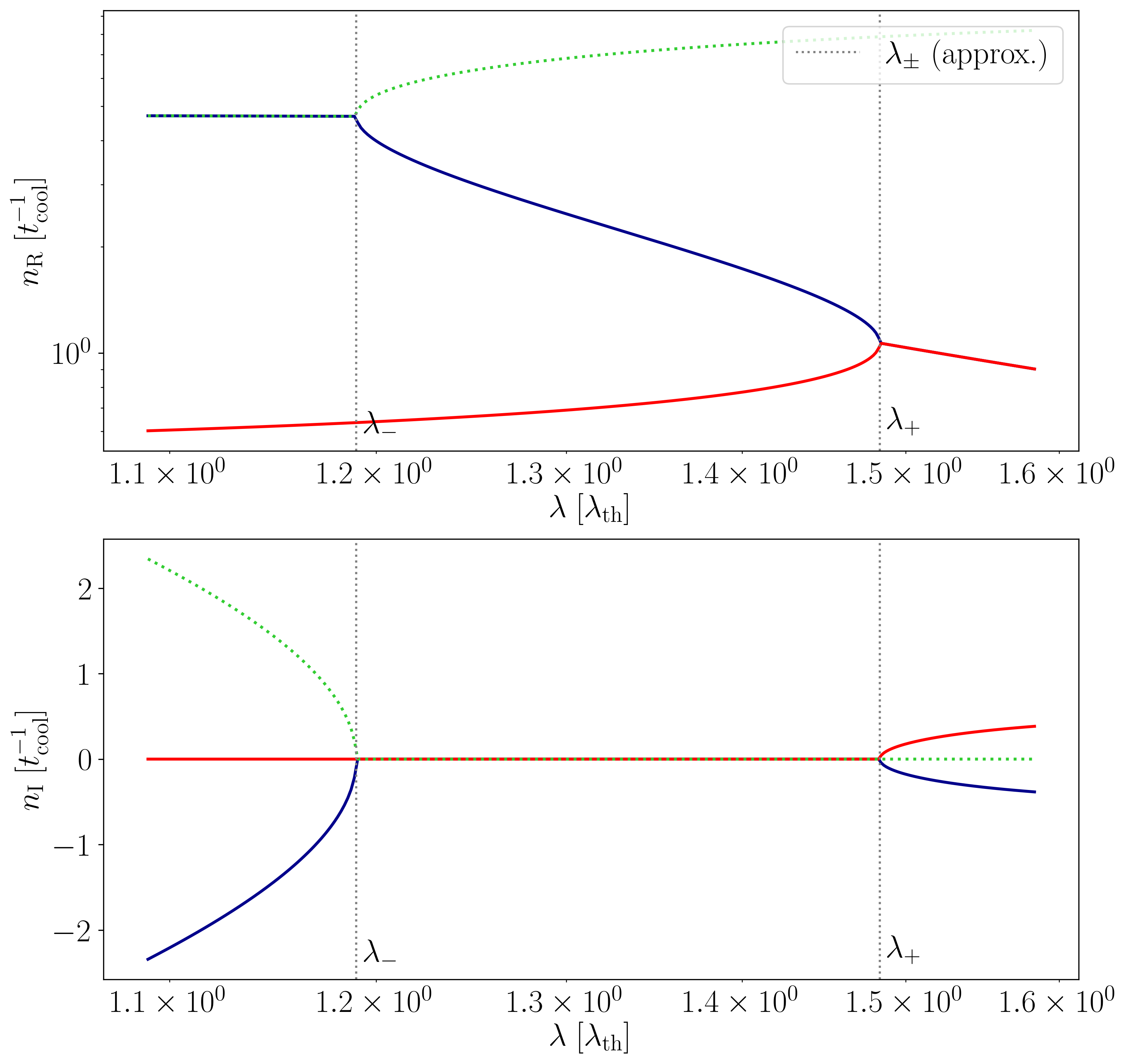
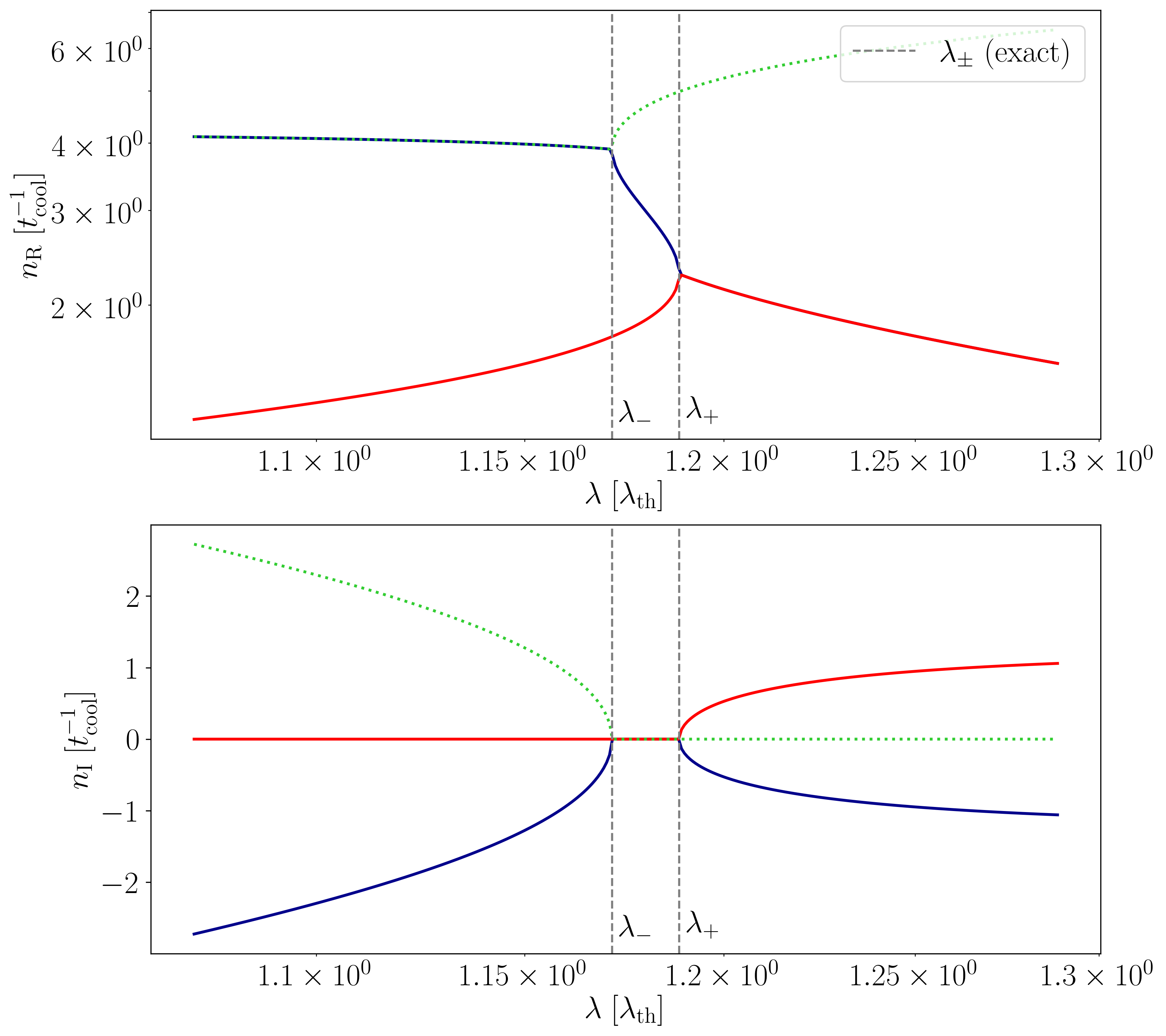
The conclusion of this subsection is that the analytical formulas for the critical wavelengths $\lambda_{\mathrm{c}}$ and $\lambda_{\pm}$ provided by Waters and Proga (2019) are good approximations to the exact ones as long as $\lambda_{\mathrm{F}}$ is small. And, what is more important, the classification of the modes supported by the system given in terms of $R$ is essentially correct. We use the word “essentially” because values of $R$ near 0, 1/9, or 1 may behave differently to what is exposed in Figure 2 of Waters and Proga (2019); Figure 2 shows an example of this.

V.2 The range $1/9<R<1/3$

In their Section 3.3, Waters and Proga (2019) state that for $1/9<R<1/3$, instead of the two critical wavelengths that are present for $0<R<1/9$ (see Figure 1), there is just one. We now explain why this claim is incorrect. This single critical wavelength should come from Equation (13) of Waters and Proga (2019). An examination of the term $1-4R/B^{2}$, with

$$B=\frac{27}{4}\left(R-\frac{1}{3}\right)^{2}-1,$$ (38)

shows that it is negative for $R$ in the range $1/9<R<1/3$; and the same happens for $1/3<R<1$. Thus, there is no critical wavelength for $1/9<R<1$ and this implies that rows 4 and 5 of Figure 2 of Waters and Proga (2019) must be merged.

V.3 Solution types for wavelengths smaller than $\simeq\lambda_{\mathrm{F}}$

At wavelengths shorter than those included in Figure 2 of Waters and Proga (2019), thermal conduction stabilizes unstable thermal modes and overstable acoustic modes. Just to give two examples, this is what happens with the unstable thermal mode (black shading) in the first row and the overstable acoustic modes (gray shading) in the second row of Table 1. Our aim in this subsection is to incorporate the wavenumbers $k_{\mathrm{therm}}$ and $k_{\mathrm{ac}}$ defined in Equations (18) and (19).

Figure 3: Number of critical wavenumbers as a function of $N_{\mathrm{p}0}$ and $N_{\rho 0}$ for a fixed $\lambda_{\mathrm{F}}/\lambda_{\mathrm{th}}$. This panel shows the cases $\lambda_{\mathrm{F}}/\lambda_{\mathrm{th}}=0.2$, 1, 5, 20, with other values of this ratio shown in the accompanying movie. The $R=1/9$ line does not appear straight because of the symmetric logarithmic scale used in both axes. (An animation of this figure is available.)

We note that $k_{\mathrm{therm}}$ exists provided that the system is isobarically unstable for $\lambda\rightarrow\infty$ ($N_{\mathrm{p}0}<0$). This happens in rows 1 and 3–6 of Table 1. In addition, $k_{\mathrm{ac}}$ exists if $R-1$ and $N_{\rho 0}$ have the same sign, i.e., in rows 2–5 and 7 of the same table. Hence, both wavenumbers exist in rows 3–5 ($0<R<1$). It can be easily proved that the corresponding wavelengths, $\lambda_{\mathrm{therm}}$ and $\lambda_{\mathrm{ac}}$, satisfy $\lambda_{\mathrm{ac}}<\lambda_{\mathrm{therm}}$ if $0<R<1/\gamma$ and $N_{\mathrm{p}0},N_{\rho 0}<0$ or if $1/\gamma<R<1$ and $N_{\mathrm{p}0},N_{\rho 0}>0$; this last possibility is irrelevant for the stability of the system because all modes are attenuated for all wavelengths. Taking $\gamma=5/3$, we see that $\lambda_{\mathrm{ac}}<\lambda_{\mathrm{therm}}$ in rows 3 and 4, whereas in row 5 the opposite applies, namely $\lambda_{\mathrm{therm}}<\lambda_{\mathrm{ac}}$. Of course, for $R=1/\gamma\equiv 3/5$ we have $\lambda_{\mathrm{ac}}=\lambda_{\mathrm{therm}}$ and all three modes transition between stable and unstable at the same wavelength.

The summary of this subsection is that, to extend Figure 2 of Waters and Proga (2019) all the way to $\lambda=0$, it is necessary to include the possible mode stabilization that takes place at $\lambda_{\mathrm{ac}}$ and $\lambda_{\mathrm{therm}}$. Table 1 corrects and expands Figure 2 of Waters and Proga (2019) according to the issues discussed in this section. Section VI contains plots of $n_{\mathrm{R}}$ and $n_{\mathrm{I}}$ versus $\lambda$ for the values of $R$ in each range of Table 1.

V.4 Instability domains for arbitrary $\lambda_{\mathrm{F}}$

In Section V.1 we have concluded that Table 1 is correct as long as $\lambda_{\mathrm{F}}$ is small. But what does small $\lambda_{\mathrm{F}}$ mean? To answer this question, we solve Equation (37) on a grid of values of $N_{\mathrm{p}0}$ and $N_{\rho 0}$ for a set of values of $\lambda_{\mathrm{F}}$. The results are presented in Figure 3 and in its accompanying movie. We start inspecting the top left panel. The second and fourth quadrants of this figure correspond to rows 1 and 2 of Table 1, respectively, for which there is only one critical wavenumber (whose wavelength is $\lambda_{\mathrm{c}}$). In the third quadrant, the yellow dots are found in the region between the lines $R=0$ and $R=1/9$: this is the third row of Table 1, for which there are two critical wavenumbers (whose wavelengths are $\lambda_{-}$ and $\lambda_{+}$). In addition, the purple dots in the third quadrant show that for $R>1/9$ there are no critical wavenumbers, as shown in rows 4–7 of Table 1. It is worth recalling that $\lambda_{\mathrm{therm}}$ and $\lambda_{\mathrm{ac}}$ give the wavelengths at which the thermal and the two acoustic modes transition from stable to unstable, respectively; hence, they are not critical wavelengths in the sense given in this paper. Finally, in the first quadrant we have both $N_{\mathrm{p}0}$ and $N_{\rho 0}$ positive, a case not addressed in Table 1 because all modes are stable for all wavelengths.

As we increase $\lambda_{\mathrm{F}}/\lambda_{\mathrm{th}}$, the distribution of the number of zeros of Figure 3 remains essentially unchanged up to $\lambda_{\mathrm{F}}/\lambda_{\mathrm{th}}=1$ (see top right panel of Figure 3). For this reason, we identify “small $\lambda_{\mathrm{F}}$” with $\lambda_{\mathrm{F}}/\lambda_{\mathrm{th}}\lesssim 1$. For $\lambda_{\mathrm{F}}/\lambda_{\mathrm{th}}=2$ the deviation from the plot for $\lambda_{\mathrm{F}}/\lambda_{\mathrm{th}}=0.2$ is notable in the first quadrant and, moreover, many red dots appear in the second quadrant, meaning that, for some values of $N_{\mathrm{p}0}$ and $N_{\rho 0}$, there are mode conversions between acoustic and thermal modes at three critical wavelengths. It is not the purpose of this work to analyze in detail the stability of modes in these cases; it is enough to state that Table 1 is no longer valid for $\lambda_{\mathrm{F}}/\lambda_{\mathrm{th}}\gtrsim 1$ because the various regions in Figure 3 are not limited by $R=const.$ lines. To understand the presence of these three critical wavenumbers, we note that Equation (37) is a quartic polynomial in $k_{\mathrm{c}}^{2}$, hence it admits up to four pairs of real solutions.

Continuing to even larger values of the Field length (see bottom panels of Figure 3 and the accompanying movie), we notice that the area with three critical wavenumbers becomes the largest for $\lambda_{\mathrm{F}}/\lambda_{\mathrm{th}}\simeq 7-20$ and starts to disappear for $\lambda_{\mathrm{F}}/\lambda_{\mathrm{th}}\simeq 100$, after which the third quadrant contains mostly systems with two critical wavenumbers.

VI Growth rate and dispersion diagrams

The purpose of this section is to present plots of $n_{\mathrm{R}}$ and $n_{\mathrm{I}}$ versus $\lambda$ for values of $N_{\mathrm{p}0}$ and $N_{\rho 0}$ representative of each row of Table 1. A symmetric logarithmic scale is used in the vertical axis and for this reason the curves show a kink when $n_{\mathrm{R}}/t_{\mathrm{cool}}$ or $n_{\mathrm{I}}/t_{\mathrm{cool}}$ enter the range $~[-10,10]$. No assumptions are made on the heat-loss function. Both $n_{\mathrm{R}}$ and $n_{\mathrm{I}}$ are non-dimensionalized against $1/t_{\mathrm{cool}}$ and all wavelengths are non-dimensionalised against $\lambda_{\mathrm{th}}=c_{\mathrm{s}}t_{\mathrm{cool}}$. The asymptotic formulas for $\lambda\rightarrow 0$ (Equations (27) and (29)) and $\lambda\rightarrow\infty$ (Equations (31), (33), and (35)) included in the plots are presented in Sections III and IV. In our plots we have only used the dominant terms of the thermal mode formulas, although considering all terms yields an agreement with the exact values over a larger wavelength range. Finally, we have taken $\lambda_{\mathrm{F}}/\lambda_{\mathrm{th}}=0.2$ and $\gamma=5/3$ in all calculations.

Figure 4: Case $R<0$, $N_{\rho 0}>0$, $N_{\mathrm{p}0}<0$. Top and bottom panels: real and imaginary parts of the growth rate versus wavelength. The solid blue, solid red, and dotted green lines are the three solutions of the dispersion relation. The legends refer to the asymptotic curves in the limits $\lambda\rightarrow 0$ (dominant term of Equation (27) and Equation (29)) and $\lambda\rightarrow\infty$ (dominant terms of Equations (31) and (33)). The vertical gray dotted lines mark the position of the relevant wavelengths, the horizontal grey dotted line in the top panel corresponds to $n_{\mathrm{R}}=0$. The parameter values are $N_{\rho 0}=10$, $R=-2$, and $\lambda_{\mathrm{F}}=0.2\lambda_{\mathrm{th}}$.

Figure 5: As in Figure 4 but for case $R<0$, $N_{\rho 0}<0$, $N_{\mathrm{p}0}>0$. The legends refer to the asymptotic curves in the limits $\lambda\rightarrow 0$ (dominant term of Equation (27) and Equation (29)) and $\lambda\rightarrow\infty$ (dominant terms of Equations (31) and (33)). The parameter values are $N_{\rho 0}=-10$, $R=-2$, and $\lambda_{\mathrm{F}}=0.2\lambda_{\mathrm{th}}$.

Other significant wavelengths are $\lambda_{\mathrm{therm}}$ and $\lambda_{\mathrm{ac}}$, that mark the change of the thermal and acoustic modes from damped to exponentially growing, and $\lambda_{\mathrm{c}}$ (case $R<0$) and $\lambda_{\pm}$ (case $0<R<1/9$), that signal the transition between a pair of acoustic modes and two thermal modes; they are obtained by solving Equation (37).

We begin our discussion with a plasma configuration that is isobarically unstable and isochorically and isentropically stable: see row 1 of Table 1 and Figure 4. Starting at small wavelengths, we find a characteristic that is common to all values of $R$: there is one thermal and two acoustic waves, all stable, whose growth rates are well reproduced by Equations (27) and (29). Since the system is isentropically stable, acoustic modes are stable for all wavelengths and this is the reason why $\lambda_{\mathrm{ac}}$ (Equation (19)) does not appear in this row of Table 1. On the other hand, the thermal mode becomes unstable at $\lambda=\lambda_{\mathrm{therm}}$ (see Equation (18)), after which $n_{\mathrm{R}}$ reaches a maximum, at a wavelength that is denoted by $\lambda_{\mathrm{m}}$. Field (1965) gave an approximate expression for the corresponding wavenumber, $k_{\mathrm{m}}$, but here we prefer to compute it analytically. To do so, we take the derivative with respect to $k$ of Equation (6) with $n$ substituted by $n_{\mathrm{R}}$ and, upon imposing $dn_{\mathrm{R}}/dk=0$, we obtain

$$k_{\mathrm{m}}^{2}=-\frac{k_{\mathrm{F}}^{2}}{2c_{\mathrm{s}}^{2}}\left(\frac{\gamma n_{\mathrm{R}}^{2}}{k_{\mathrm{F}}^{2}}+\gamma t_{\mathrm{cool}}c_{\mathrm{s}}^{2}n_{\mathrm{R}}+N_{\mathrm{p}0}c_{\mathrm{s}}^{2}\right).$$ (39)

Now, this expression is inserted into Equation (6) with $n$ substituted by $n_{\mathrm{R}}$, which leads to a fourth-degree polynomial equation for $n_{\mathrm{R,max}}$, the maximum growth rate. The wavenumber at which this maximum takes place is then given by Equation (39).

At $\lambda=\lambda_{\mathrm{c}}$, the two acoustic modes transition to two stable thermal modes ($n_{\mathrm{R}}<0$, $n_{\mathrm{I}}=0$). Finally, in the large wavelength range, Equations (31) and (33) show an excellent agreement with the growth rates of the three thermal modes.

We next move to row 2 of Table 1 and Figure 5, that correspond to a plasma that is isochorically and isentropically unstable and isobarically stable. The main differences from Figure 4 are that the thermal mode is stable for all wavelengths, while the two acoustic modes first become overstable at $\lambda=\lambda_{\mathrm{ac}}$ and later switch to two unstable thermal modes at $\lambda=\lambda_{\mathrm{c}}$. These two modes remain unstable as $\lambda\rightarrow\infty$, their growth rates given by Equations (31) and (33).

Figure 6 and the third row of Table 1 present us with the most complex case in terms of wavelength ranges. Now all three stability criteria are met and, moreover, there are two critical wavelengths, $\lambda_{\mp}$, at which the two (overstable) acoustic modes transition to two (unstable) thermal modes and then back to two (overstable) acoustic modes. At wavelengths $\lambda_{\mathrm{ac}}$ and $\lambda_{\mathrm{therm}}$, smaller than $\lambda_{-}$, we find that the modes shift from damped to undamped, as discussed above. And at wavelengths larger than $\lambda_{+}$ the growth rates behave as predicted by Equations (31) and (35).

Figure 6: As in Figure 4 but for case $0<R<1/9$, $N_{\rho 0},N_{\mathrm{p}0}<0$. The legends refer to the asymptotic curves in the limits $\lambda\rightarrow 0$ (dominant term of Equation (27) and Equation (29)) and $\lambda\rightarrow\infty$ (dominant term of Equation (31) and Equation (35)). The parameter values are $N_{\rho 0}=-10$, $R=0.05$, and $\lambda_{\mathrm{F}}=0.2\lambda_{\mathrm{th}}$.

Next, we discuss together rows 4 and 5 of Table 1 and their corresponding Figures 7 and 8 because they only differ in the ordering of $\lambda_{\mathrm{therm}}$ and $\lambda_{\mathrm{ac}}$. In both cases we find isobaric, isochoric, and isentropic instability, and for this reason both the thermal mode and the pair of acoustic modes become unstable/overstable at sufficiently large wavelengths. Given that there are no critical wavenumbers, we find no mode conversions between the two mode types, and both modes have growth rates that tend to their asymptotic Equations (31) and (35).

Figure 7: As in Figure 4 but for case $1/9<R<1/\gamma$, $N_{\rho 0},N_{\mathrm{p}0}<0$. The legends refer to the asymptotic curves in the limits $\lambda\rightarrow 0$ (dominant term of Equation (27) and Equation (29)) and $\lambda\rightarrow\infty$ (dominant term of Equation (31) and Equation (35)). The parameter values are $N_{\rho 0}=-10$, $R=0.3$, and $\lambda_{\mathrm{F}}=0.2\lambda_{\mathrm{th}}$.

Figure 8: As in Figure 4 but for case $1/\gamma<R<1$, $N_{\rho 0},N_{\mathrm{p}0}<0$. The legends refer to the asymptotic curves in the limits $\lambda\rightarrow 0$ (dominant term of Equation (27) and Equation (29)) and $\lambda\rightarrow\infty$ (dominant term of Equation (31) and Equation (35)). The parameter values are $N_{\rho 0}=-10$, $R=0.8$, and $\lambda_{\mathrm{F}}=0.2\lambda_{\mathrm{th}}$.

Row 6 of Table 1 and Figure 9 show a thermal mode that becomes unstable at $\lambda=\lambda_{\mathrm{therm}}$, because both the isobaric and isochoric criteria are satisfied. This mode reaches a maximum value of $n_{\mathrm{R}}$ before tending to the value given by Equation (31). With regard to the acoustic modes, they are stable for all wavelengths because the system is isentropically stable.

Figure 9: As in Figure 4 but for case $R>1$, $N_{\rho 0},N_{\mathrm{p}0}<0$. The legends refer to the asymptotic curves in the limits $\lambda\rightarrow 0$ (dominant term of Equation (27) and Equation (29)) and $\lambda\rightarrow\infty$ (dominant term of Equation (31) and Equation (35)). The parameter values are $N_{\rho 0}=-10$, $R=2$, and $\lambda_{\mathrm{F}}=0.2\lambda_{\mathrm{th}}$.

Row 7 of Table 1 is analogous to row 6, but now the roles of the thermal and the acoustic modes are interchanged: the former is stable for all $\lambda$ and the latter are overstable for $\lambda>\lambda_{\mathrm{ac}}$. See Figure 10.

Figure 10: As in Figure 4 but for case $R>1$, $N_{\rho 0},N_{\mathrm{p}0}>0$. The legends refer to the asymptotic curves in the limits $\lambda\rightarrow 0$ (dominant term of Equation (27) and Equation (29)) and $\lambda\rightarrow\infty$ (dominant term of Equation (31) and Equation (35)). The parameter values are $N_{\rho 0}=10$, $R=2$, and $\lambda_{\mathrm{F}}=0.2\lambda_{\mathrm{th}}$.

VII Do truly isobaric perturbations exist?

In Sections III and IV we have seen that, under certain circumstances, truly isochoric perturbations are allowed: this happens for the thermal mode when either $\lambda\rightarrow 0$ or $\lambda\rightarrow\infty$. This leads us to wonder whether purely isobaric perturbations exist. According to Equation (22), this requires $n/k=0$. Of course, whenever $k$ is finite and the growth rate of the thermal mode vanishes, the perturbations $\delta p$ and $\delta v$ also vanish, and the system has sinusoidal density and temperature perturbations that do not change in time. This takes place at the wavenumber $k_{\mathrm{therm}}$, given by Equation (18), at which the thermal mode changes from being evanescent to being amplified.

Apart from this trivial solution, all other wavelengths produce pressure perturbations. Nevertheless, a truly isobaric thermal mode exists in the absence of conduction. Indeed, if $\kappa=0$ and $\lambda\rightarrow 0$, the thermal mode has the growth rate

$$n_{\mathrm{R}}=-\frac{N_{\mathrm{p}0}}{\gamma t_{\mathrm{cool}}},\hskip 56.9055ptn_{\mathrm{I}}=0.$$ (40)

Given that $n/k\rightarrow 0$ as $\lambda\rightarrow 0$, this mode only gives rise to density and temperature perturbations, but in this case they grow in time if the system is isobarically unstable ($N_{\mathrm{p}0}<0$), otherwise they are damped. Equation (40) corresponds to Equation (31) of Field (1965). For completeness, we also give the growth rate of acoustic modes for $\kappa=0$ and $\lambda\rightarrow 0$,

$$n_{\mathrm{R}}=\frac{N_{\rho 0}}{2t_{\mathrm{cool}}}(R-1),\hskip 56.9055ptn_{\mathrm{I}}=\pm kc_{\mathrm{s}},$$ (41)

which corresponds to Equation (32) of Field (1965).

In spite of these results, a uniform and infinite plasma with thermal conduction can support a thermal mode with an almost isobaric perturbation. For each of the seven representative parameter values used in Figures 4–10, there is a wavelength range, roughly between $0.01\lambda_{\mathrm{th}}$ and $0.1\lambda_{\mathrm{th}}$, for which the pressure perturbation is much smaller than that of the density and temperature (all normalized to their equilibrium values). This wavelength range is the smallest in rows 3 and 7 of Table 1, that are the two cases in which the system is isobarically stable. For shorter and longer wavelengths than those mentioned in this paragraph, the thermal mode transitions to an isochoric behavior. In general, for all seven cases of Table 1, the thermal mode is essentially isochoric for $\lambda\lesssim 10^{-3}\lambda_{\mathrm{th}}$ and for $\lambda\gtrsim\lambda_{\mathrm{th}}$. Of course, it is always stable if $\lambda<\lambda_{\mathrm{therm}}$ and is unstable for $\lambda>\lambda_{\mathrm{therm}}$ in all instability domains but the last in Table 1.

VIII Conclusions

We have revisited the linear modes of an infinite and homogeneous hydrodynamic medium, investigated by Field (1965) and Waters and Proga (2019). In this work we have imposed no particular form of the heating and radiative cooling processes and have only assumed Spitzer’s expression for parallel thermal conductivity. We find that the presentation of the different regimes of linear thermal instability given in Figure 2 of Waters and Proga (2019) is easier to understand than in Figure 1 of Field (1965). Nevertheless, the former contains an error that has been corrected (namely the relevance of the value $R=1/3$) and some necessary additions that have been included in our Table 1 (namely incorporating the wavelengths $\lambda_{\mathrm{therm}}$ and $\lambda_{\mathrm{ac}}$ and thermal conduction). This table gives a comprehensive summary of all domains of thermal instability, making clear which modes are present in different wavelength ranges and whether they are unstable or damped. The domains of instability are separated by critical values of $R$ that were derived by Waters and Proga (2019) under the assumption of vanishing Field length ($\lambda_{\mathrm{F}}\rightarrow 0$), or equivalently, in the limit of no thermal conduction. The physical meaning of $R$ comes from its definition as the quotient $N_{\mathrm{p}0}/(\gamma N_{\rho 0})$, where $N_{\mathrm{p}0}<0$ and $N_{\rho 0}<0$ are a dimensionless form of the isobaric and isochoric instability criteria obtained by Field (1965). Including thermal conduction in the analysis implies that the critical values of $R$ can shift slightly and we have shown that Table 1 and the auxiliary Figures 4–10 remain an excellent guide to the domains of instability of a hydrodynamic plasma for which $\lambda_{\mathrm{F}}\lesssim\lambda_{\mathrm{th}}$. For larger values of the Field length, however, the instability domains have no simple description in terms of $R$.

Furthermore, we have presented a detailed analysis of the modes of the homogeneous hydrodynamical system studied by Field (1965) and Waters and Proga (2019) for very short and very long wavelengths. We have also shown that, to study the perturbations caused by modes with an isochoric evolution, it is essential to express all perturbations in terms of the amplitude of the pressure perturbation instead of the amplitude of the density perturbation. When $\lambda\rightarrow 0$, the thermal mode becomes isochoric. It has no velocity perturbation, and the temperature and pressure perturbations damp by heat exchange via thermal conduction. Moreover, there is a pair of damped isothermal acoustic modes that propagate in opposite directions at the isothermal sound speed.

Equation (16) of Seno et al. (2026) provides an approximation to the asymptotic behavior of the growth rate of the thermal mode for small wavelength. In terms of the parameters used in this paper, this equation can be written as

$$n_{\mathrm{R}}=-\frac{N_{\rho 0}}{\gamma t_{\mathrm{cool}}}+\frac{c_{\mathrm{s}}}{\gamma}-\frac{1}{\gamma t_{\mathrm{cool}}}\left(\frac{k}{k_{\mathrm{F}}}\right)^{2}.$$ (42)

There is a clear discrepancy between this expression and our Equation (27), the reason being that, to derive it, Seno et al. (2026) incorrectly assumed that the thermal mode is isobaric when $\lambda\rightarrow 0$. We have plotted the growth rate of Equation (42) in Figures 4–10 and have verified that Seno et al.’s approximation is not too far from the red curve of the top panel for $\lambda\simeq 10^{-2}\lambda_{\mathrm{th}}$, but it departs from the actual behavior of $n_{\mathrm{R}}$ for smaller wavelengths. Hence, Equation (42) does not provide a valid estimate of $n_{\mathrm{R}}$ for $\lambda\rightarrow 0$, while Equation (27) does.

When $\lambda\rightarrow\infty$ another isochoric thermal mode is present, its stability being governed by the isochoric stability criterion. Thermal conduction plays no role in the exponential damping/growth of this mode. When the parameter $R$ is negative, this thermal mode is accompanied by two additional thermal modes with growth rate $\pm\sqrt{R}c_{\mathrm{s}}$ (see Waters and Proga, 2019). When $R>0$, these two thermal modes are replaced by a pair of acoustic solutions with phase speed $\pm\sqrt{R}c_{\mathrm{s}}$ that are stable either if $R>1$ and the isochoric stability criterion is fulfilled or if $R<1$ and the isochoric stability criterion is not fulfilled.

Figure 11: Top: optically thin coronal radiative losses from the CHIANTI atomic database. Two lines with power-law slopes of $-2$ (purple) and $-3$ (blue) are shown for comparison purposes. Bottom: $R$ as a function of temperature. The horizontal dashed line corresponds to $R=1$.

The amplitudes of the perturbed variables in the linear regime (see Equations (20)–(26)) are such that, when thermal conduction is included, perturbations of the medium always produce pressure and density changes. In other words, truly isobaric and isochoric perturbations are not allowed, and this is true regardless of whether the medium is isobarically or isochorically unstable for $\lambda\rightarrow\infty$ ($N_{\mathrm{p}0}<0$ or $N_{\rho 0}<0$) or not. On the other hand, the medium supports a thermal mode with isochoric perturbation both for $\lambda\rightarrow 0$ and $\lambda\rightarrow\infty$. Isochoric perturbations were discarded by Field (1965) on the basis that “pressure variations accompanying isochoric temperature variations will in general drive motions which destroy the constancy of density”. This sentence is concluded as follows, “so that this criterion is incompatible with the force equation.” We have shown that this incompatibility does not exist for very small and very long wavelengths. Furthermore, if we relax the condition on the thermal mode to be purely isobaric or isochoric, we find that it is almost isochoric for very small or very large wavelengths and is almost isobaric for intermediate wavelengths. For example, for $\lambda_{\mathrm{F}}=0.2\lambda_{\mathrm{th}}$, the thermal mode is almost isochoric for $\lambda\lesssim 10^{-3}\lambda_{\mathrm{th}}$ and for $\lambda\gtrsim\lambda_{\mathrm{th}}$ and almost isobaric for $0.01\lambda_{\mathrm{th}}\lesssim\lambda\lesssim 0.1\lambda_{\mathrm{th}}$. We also find that increasing $\lambda_{\mathrm{F}}$ results in a reduction of the range of $\lambda$ for which the thermal mode is almost isobaric, together with a shift to higher wavelengths. For example, for $\lambda_{\mathrm{F}}=\lambda_{\mathrm{th}}$, this range becomes $0.1\lambda_{\mathrm{th}}\lesssim\lambda\lesssim\lambda_{\mathrm{th}}$ for all rows of Table 1, except rows 2 and 7, for which the thermal mode behaves almost isochorically for all wavelengths.

Growth rate and dispersion diagrams are presented in Section VI for all the domains of instability. These diagrams provide a graphical counterpart to Table 1 and give evidence of how the conversion between thermal and acoustic modes takes place, how the modes behave for very small or very large wavelengths, in what wavelength ranges there is instability, etc. A discussion of the instability domains in terms of $N_{\mathrm{p}0}$, $N_{\rho 0}$, and $\lambda_{\mathrm{F}}/\lambda_{\mathrm{th}}$ is given in Section V.4. Figure 3 and its accompanying movie can be considered a simplification of Figure 1 of Field (1965): the former provides the number of critical wavenumbers in three dimensions (with $\lambda_{\mathrm{F}}/\lambda_{\mathrm{th}}$ represented along the third axis) and, at the same time, does not involve the wavenumber, which is present in the latter.

In a follow-up of this paper we plan to investigate the non-linear saturation regime of one-dimensional hydrodynamics in the presence of a source term in the energy equation, incorporating constant heating, radiative losses, and temperature-dependent thermal conduction. The aim is to understand the behavior that follows the excitation of the thermal mode or the acoustic modes beyond the linear phase. In addition, although thermal instability in a homogeneous plasma threaded by a uniform magnetic field has already been explored (e.g., Field, 1965; Claes and Keppens, 2019; Falle et al., 2020), it remains to examine the possible classification of its instability domains in terms of a few parameters. All of these studies should be relevant to laboratory plasmas in addition to astrophysical ones.

We end his work with a discussion of the catastrophic cooling (CC) instability recently proposed by Waters and Stricklan (2025) as the agent causing coronal rain plasma condensations. We have already made clear that the CC solution coincides with the thermal mode in the $\lambda\rightarrow\infty$ limit. Obviously, a comparison between linear thermal instability in a homogeneous medium and coronal rain formation must be taken with a grain of salt because thermal conduction plays a major role in the unperturbed, non-uniform coronal loop equilibrium and this can affect perturbations in ways that are not captured by the Field length. Waters and Stricklan (2025) argued that for $0<R<1$ the CC mode is the fastest growing linear mode and that, as a consequence, it will be the first to reach non-linearity and will then dominate the evolution of the system. This is in line with Figures 6–8, which show that the highest growth rate of the thermal mode occurs as $\lambda\rightarrow\infty$, exclusively when $0<R<1$. However, for typical coronal loop conditions, $R$ does not lie in this range. The top panel of Figure 11 presents the optically thin radiative losses based on the CHIANTI atomic database (Dere et al., 1997; Dufresne et al., 2024), with the corresponding $R$ shown in the bottom panel of this figure. We can see that $R>1$ for all temperatures in the range $\simeq$ 1–3 MK, typical of active region coronal loops hosting coronal rain. The result $R>1$ becomes obvious with the help of Equation (A3), that tells us that the slope of $Q(T)$ must be greater than 3 in absolute value to achieve $R<1$. In the case of Figure 11, $Q(T)$ has a negative slope with a maximum absolute value around 2.6; at this point is worth noticing that other commonly used coronal cooling functions have slopes around 1.5. Then, the conclusion is that the coronal plasma is better represented by $R>1$, i.e., the sixth row of Table 1 and Figure 9, which implies that the thermal mode achieves its maximum growth rate at a finite wavelength rather than for $\lambda\rightarrow\infty$.

Appendix A Power-law cooling function

In the optically thin solar corona, the heat loss rate per unit volume is

$$\rho\Lambda(T)=n_{\mathrm{e}}n_{\mathrm{H}}Q(T),$$ (A1)

where $n_{\mathrm{e}}$ is the electron density and $n_{\mathrm{H}}$ is the density of protons and hydrogen atoms. Let us assume that $Q(T)$ can be expressed as a power-law function of temperature. Then,

$$Q(T)=\alpha T^{-\beta}.$$ (A2)

Assuming a fully ionized hydrogen plasma, with $n=n_{\mathrm{e}}=n_{\mathrm{H}}$, $\rho\simeq m_{\mathrm{p}}n$, and $m_{\mathrm{p}}$ the proton mass, the following expressions apply,

$$N_{\rho 0}=-\beta,\hskip 28.45274ptN_{\mathrm{p}0}=-(\beta+2),\hskip 28.45274ptR=\frac{\beta+2}{\gamma\beta}.$$ (A3)

Other relevant quantities are

$$k_{\mathrm{F}}=\left(\frac{\alpha}{\kappa_{0}}\right)^{1/2}\frac{n_{0}}{T_{0}^{\beta/2+7/4}},\hskip 28.45274ptt_{\mathrm{cool}}=\frac{2k_{\mathrm{B}}}{(\gamma-1)\alpha}\frac{T_{0}^{\beta+1}}{n_{0}},$$ (A4)

$$\lambda_{\mathrm{th}}=t_{\mathrm{cool}}c_{\mathrm{s}}=\left(\frac{2\gamma k_{\mathrm{B}}}{m_{\mathrm{p}}}\right)^{1/2}\frac{2k_{\mathrm{B}}}{(\gamma-1)\alpha}\frac{T_{0}^{\beta+3/2}}{n_{0}},$$ (A5)

where $k_{\mathrm{B}}$ is the Boltzmann constant and $T_{0}$, $n_{0}$ are the unperturbed temperature and number density.