Continuum-statistical dynamics of colloidal suspensions under kinematic reversibility

Abstract

We present a continuum-statistical linear response theory of colloidal motion rooted in the principle of kinematic reversibility. By decoupling hydrostatic and hydrodynamic stress, we show that an explicit form of the colloidal flux can be derived in terms of thermodynamic forces and auxiliary flows when the Lorentz reciprocal theorem is applied to continuum-mechanical momentum fluctuations. Our framework bridges the conceptual gap between continuum-mechanical and non-equilibrium thermodynamic reciprocal relations and provides a unified description of transport phenomena such as force-free phoretic motion, active swimming and buoyant sedimentation. Furthermore, our results predict two transport mechanisms that do not fit into the traditional picture of interfacial force-free motion. The first arises from hydrodynamic drag induced by the excess weight of fluid, while the second results from thermodynamic force fluctuations in the absence of interfacial excess. Owing to its linear character, our continuum-statistical framework may also be used numerically to determine transport coefficients of dense colloidal suspensions without explicitly resolving the underlying microhydrodynamics.

1 Introduction

Continuum mechanics describes a multicomponent system in terms of continuous media that meet at well-defined boundaries, by partitioning the system into a fine mesh of elementary volumes, each statistically homogeneous in the thermodynamic limit. The size $dV$ of an elementary volume defines the continuum scale. Once this scale is identified, the dynamics is governed by conservation laws in the form of differential continuity equations for mass, particle number, momentum and energy, expressed in terms of fluxes and source densities defined throughout these media. A continuous object, composed of such a medium and suspended in another medium, then experiences continuum mechanical forces that can be computed through the corresponding continuity equations.[24]

These equations are closed by assuming that each elementary volume is in local thermodynamic equilibrium, yielding linear constitutive relations between fluxes and gradients of certain thermodynamic and hydrodynamic continuum fields.[20] Within Onsager’s theory of non-equilibrium thermodynamics, time-reversal symmetry implies that the transport coefficients in these relations are symmetric, a result known as the Onsager reciprocal relations.[33, 34] However, in non-equilibrium thermodynamics these coefficients are phenomenological quantities, dependent on molecular dynamic correlations and hence only inferable from experiments or from molecular dynamical simulations. This presents a limitation for describing the dynamics in colloidal suspensions, where molecular-level modeling is impractical.

To overcome this limitation, Derjaguin considered modeling the constituent particles of a medium as continuous objects on their own, thus obtaining continuum-mechanical expressions of transport coefficients based on Onsager reciprocal symmetry.[18] This approach reduces the phenomenological character of coupling in the low Knudsen number regime, where the molecular dynamic effect on transport can be described by a set of well-defined boundary conditions. Since continuity equations are in general not time-reversal symmetric, a shortcoming of such Onsager reciprocal approaches is that they often overlook the condition required to recover a reciprocal symmetry on the continuum scale.[14, 1] This condition, also known as the principle of kinematic reversibility, is usually justified from a continuum-mechanical perspective. In contrast, continuum-mechanical treatments usually focus on the hydrodynamic aspect of reciprocal relations, whereas underlying driving forces are often modeled phenomenologically within a boundary layer approximation, based on an effective slip velocity[37] or interfacial tension gradient.[29] However, some driving forces, such as those responsible for phoretic motion, do not require phenomenological modeling because they can be related to thermodynamic equations of state. For the motion of a colloid whose diameter is comparable to the thickness of its interfacial interaction layer, it is then necessary to study the coupling between these local thermodynamic forces and flows beyond the boundary layer approximation.[35, 15]

Reducing the phenomenological character of colloidal transport, and closing the gap between continuum-mechanical and non-equilibrium thermodynamic reciprocal approaches, thus remains a conceptually challenging area of active research.[39, 11] Here, we show that bridging this gap relies on a rigorous treatment of hydrostatic forces, whose fluctuations satisfy an overall force-free condition. Our approach, which is based on the application of the Lorentz reciprocal theorem to these continuum-mechanical momentum fluctuations, offers a clear perspective on the underlying assumptions of kinematic reversibility, the solvent’s role in momentum relaxation, and the driving forces of diffusion and advection in colloidal suspensions. First, this approach is used to derive a continuum-mechanical expression for the velocity of a single colloid. It is then applied to a homogeneous, isotropic suspension to obtain a continuum-statistical expression for the colloidal diffusion flux.

2 Colloidal Suspensions: Definitions and Properties

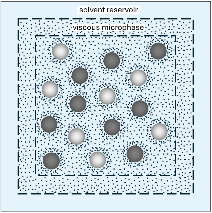
The system under consideration is a volume-filling, incompressible colloidal suspension, which may include chemical or thermal sources, but must conserve mass internally. The local microdynamics is described continuum-mechanically, relative to an inertial laboratory frame. A non-equilibrium force is a force arising from non-equilibrium boundary conditions, whereas an equilibrium quantity, denoted by a subscript ”eq”, is a quantity evaluated in the absence of such forces. Moreover, we refer to a collection of indistinguishable particles of a given chemical species as a component of the suspension, and define a microphase as a continuous medium composed of a combination of such components.

As shown in Fig. 1, the suspension consists of different species of microparticles and small solutes dispersed in a solvent reservoir, such that within a representative region $\mathcal{V}$ of the suspension, we have $N_{\lambda}\ll N_{k}\ll N_{l}$, where $N_{\lambda}$ is the number of microparticles of any microparticle species $\lambda$, $N_{k}$ is the number of particles of any solute component $k$, and $N_{l}$ is the number of particles of any solvent component $l$. The solvent, and the small solutes suspended in it, constitute an isotropic viscous microphase, whereas the microparticles consist of solid microphases, made of chemically bound components that do not support viscous shear or diffusion. The viscous microphase meets the microparticles at well-defined interfacial boundaries, where it remains isotropic assuming that molecular crowding and orientational correlations can be ignored. The colloids are a chosen species of microparticles whose motion we seek to determine, whereas the fluid refers to the surrounding viscous microphase and all other microparticle species suspended in it. The principle of kinematic reversibility is based on a low Knudsen number, low Reynolds number, and low Mach number. The solvent is therefore modeled as a strongly coupled molecular medium that forms a thermodynamic reservoir, rapidly responding to non-equilibrium forces to maintain a mechanical equilibrium under incompressible shear flow.

For kinematic reversibility, we also require that two distinct flow fields considered inside the same region occur under the same dynamic viscosity and component number densities. This does not imply spatial uniformity of these quantities, but rather that they remain unchanged under different force fields. The condition of local thermodynamic equilibrium must therefore hold not only at the continuum scale of $dV$, but also at the macroscopic scale of a representative region $\mathcal{V}$ of the suspension. This condition, which we refer to as the condition of representative local thermodynamic equilibrium (RLTE), implies that the dynamics of boundaries is slow compared to the relaxation dynamics of local continuum fields and allows for an equilibrium-statistical consideration of local component distributions, as depicted for a single colloid in Fig. 2b. Consequently, interfacial regions, which contain an excess of free energy due to interfacial potential interactions, can be considered at equilibrium, and the local dynamics inside a microphase decouples into a description of its effective reservoir components only.[21, 36, 26]

Figure 1: Schematic representation of a suspension. The dark and light gray spheres represent different species of microparticles, suspended in a viscous microphase. The viscous microphase consists of small solutes (black dots) dispersed in a solvent reservoir. The dashed lines represent thermodynamic reservoir boundaries.

3 Local continuity equations

At RLTE, local continuity equations can hence be solved under quasi-stationary boundary conditions on the internal and external boundaries of a representative region $\mathcal{V}$. At mechanical equilibrium and under incompressible flow, the local momentum continuity equation is given by[24]

$$\bm{f}+\nabla\cdot\bm{\sigma}=0,$$ (1)

where $\bm{f}$ is the body force density and $\bm{\sigma}$ is the stress tensor. This equation is solved under the constraint of incompressible flow, expressed by

$$\nabla\cdot\bm{u}=0,$$ (2)

where the flow velocity $\bm{u}$ is the barycentric velocity of an elementary volume $dV$.

The number density of an effective reservoir, denoted by a superscript ”$r$” and not to be confounded with a thermodynamic reservoir, can be defined locally for any component in the limit where interfacial potential interactions are absent. Denoting the interfacial interaction potentials collectively by $\left\{\phi_{j}\right\}$, where $j$ is an index over all components, the effective reservoir number density of a component $i$ is thus given by $n_{i}^{r}=n_{i}\left(\left\{\phi_{j}\right\}=0\right)$, where $n_{i}$ is the local number density of component $i$. Hence, the corresponding particle number continuity equation takes the form[20]

$$\frac{\partial n_{i}^{r}}{\partial t}+\nabla\cdot\bm{J}_{i}=\Gamma_{i},$$ (3)

where $\bm{J}_{i}$ is the net particle flux of component $i$, and $\Gamma_{i}$ is the corresponding chemical source density accounting for local production or annihilation of particles due to chemical reactions. The reservoir number density $n_{i}^{r}$ is sensitive to non-equilibrium boundary conditions, but independent of interfacial potential interactions. Furthermore, the particle flux $\bm{J}_{i}$ can be expressed as

$$\bm{J}_{i}=n_{i}^{r}\bm{u}+\bm{j}_{i},$$ (4)

where $\bm{j}_{i}$ is the local diffusion flux of component $i$. The diffusion fluxes are related via $\sum_{i}m_{i}\bm{j}_{i}=0$, where $m_{i}$ is the mass of a particle of component $i$. If the index $i$ refers to a component of a solid microphase, where diffusion is prohibited, we simply have $\bm{j}_{i}=0$. Using Eqs. (4) and (2), Eq. (3) can also be written as $\partial n_{i}^{r}/\partial t+\bm{u}\cdot\nabla n_{i}^{r}+\nabla\cdot\bm{j}_{i}=\Gamma_{i}$. The term $\bm{u}\cdot\nabla n_{i}^{r}$ is of second order in the non-equilibrium forces and is therefore negligible at RLTE. When the index $i$ refers to a component of the viscous microphase, the local conservation of particle number within $\mathcal{V}$ thus reduces to a local diffusive steady-state condition, of the form

$$\nabla\cdot\bm{j}_{i}=\Gamma_{i}.$$ (5)

In colloidal suspensions, energy transport occurs primarily via heat conduction and is much faster than the transport of particles. Conservation of energy can therefore be described using the steady-state form of the heat equation:

$$\nabla\cdot\bm{j}_{q}=Q,$$ (6)

where $Q$ is the heat source density and $\bm{j}_{q}=-\kappa\nabla T$ is the conductive heat flux, which couples to the gradient in temperature $T$ via the thermal conductivity $\kappa$.

4 Thermodynamic forces and hydrodynamic stress in colloidal suspensions

To bridge the conceptual gap between continuum-mechanical and non-equilibrium thermodynamic reciprocal relations, we must distinguish the forces that drive motion from those that respond to motion. It is therefore necessary to decompose the stress tensor $\bm{\sigma}$ into a hydrostatic stress $\bm{\sigma}_{s}$, and a hydrodynamic stress $\bm{\sigma}_{d}$ that vanishes in a static suspension:[24]

$$\bm{\sigma}=\bm{\sigma}_{s}+\bm{\sigma}_{d}.$$ (7)

The condition of RLTE completes the principle of kinematic reversibility and justifies a linearized decomposition into thermodynamic and hydrodynamic stresses that separately obey corresponding continuity conditions. A well-known transport phenomenon relying on this decomposition is buoyancy: the buoyant force on a microparticle is determined from the hydrostatic pressure field in a static fluid and is taken to be independent of the velocity gradients that arise during sedimentation.

To obtain constitutive forms of the hydrostatic and hydrodynamic stress, we write the stress tensor $\bm{\sigma}$ as

$$\bm{\sigma}=-P\bm{I}+\bm{\Sigma},$$ (8)

where $P=\text{Tr\hskip 0.56905pt}\bm{\sigma}/3$ is the pressure, $\bm{I}$ is the identity tensor, and $\bm{\Sigma}$ is the shear stress tensor. In suspensions, $\bm{\Sigma}$ consists of a purely viscous stress $\bm{\Sigma}_{\eta}$ inside the viscous microphase, and of a solid constraint stress $\mathring{\bm{\Sigma}}$ inside the solid microphases. We can therefore write the shear stress tensor as a sum of two separate stress fields, such that $\bm{\Sigma}=\bm{\Sigma}_{\eta}+\mathring{\bm{\Sigma}}$, with $\bm{\Sigma}_{\eta}=0$ inside the microparticles, and $\mathring{\bm{\Sigma}}=0$ inside the viscous microphase. The linear constitutive relation for the viscous stress tensor under incompressible flow is given by $\bm{\Sigma}_{\eta}=\eta\bm{e}$, where $\eta$ is the dynamic viscosity of the viscous microphase, and $\bm{e}$ is the strain rate tensor, defined by $\bm{e}=\left(\nabla\bm{u}+\nabla^{\dagger}\bm{u}\right)/2$. Since the microparticles are only in direct contact with the viscous microphase and hence under isotropic hydrostatic stress, we obtain the constitutive forms

$$\bm{\sigma}_{s}=-P_{s}\bm{I},$$ (9)

$$\bm{\sigma}_{d}=-P_{d}\bm{I}+\mathring{\bm{\Sigma}}+\bm{\Sigma}_{\eta},$$ (10)

where $P_{s}$ and $P_{d}$ denote the hydrostatic and hydrodynamic pressure, respectively, such that $P=P_{s}+P_{d}$. Within the viscous microphase, the hydrodynamic pressure $P_{d}$ acts as a Lagrange multiplier to enforce incompressible flow. To examine the hydrostatic response of the solvent reservoir, we write the hydrostatic pressure $P_{s}$ as the sum of a hydrostatic solvent reservoir pressure $p$ and an osmotic pressure $\Pi$:[21]

$$P_{s}=\Pi+p.$$ (11)

The hydrostatic solvent reservoir pressure $p$ is only non-zero inside the viscous microphase, where it can enforce a hydrostatic equilibrium normal to any static boundary where momentum relaxation via viscous flow is prohibited ($\nabla\cdot\bm{\sigma}_{d}=0$). Consequently, the solvent reservoir cannot act as a driver of colloidal motion. Inside a solid microphase, where $p=0$, the osmotic pressure $\Pi$ is thus simply equal to the hydrostatic pressure. Note that a solvent component may also contribute to the local osmotic pressure if it specifically interacts with the solutes or microparticles, inducing an interfacial excess free energy of solvation.[1] For convenience, we introduce the thermodynamic force density via

$$\bm{\mathcal{F}}=\bm{f}-\nabla P_{s}.$$ (12)

With Eqs. (7) and (12), the momentum continuity equation given by Eq. (1) becomes

$$\bm{\mathcal{F}}+\nabla\cdot\bm{\sigma}_{d}=0.$$ (13)

In view of Eq. (13), a state of local hydrostatic equilibrium is thus described by the condition $\bm{\mathcal{F}}=0$. This motivates the question of how thermodynamic forces may drive motion of colloids if these are modeled as continuous, freely moving objects inside the suspension.

In a suspension at RLTE, a local balance is maintained between the body forces and pressure forces arising from interfacial potential interactions.[40] The corresponding interfacial hydrostatic equilibrium is described by[14]

$$\sum_{i}\left(n_{\text{eq},i}\nabla\phi_{i}+\frac{\partial P_{s}}{\partial\phi_{i}}\nabla\phi_{i}\right)=0,$$ (14)

where $n_{\text{eq},i}$ is the equilibrium number density of component $i$. If Eq. (14) is subtracted from Eq. (13), then the body force $\bm{F}_{i}$ on component $i$ can be understood as stemming only from external fields or non-equilibrium boundary conditions, and the hydrostatic pressure gradient $\nabla P_{s}$ in Eq. (12) is then evaluated at constant interfacial interaction potentials.[14] The body force density can hence be written as

$$\bm{f}=\sum_{i}n_{\text{eq},i}\bm{F}_{i}.$$ (15)

The non-equilibrium body force $\bm{F}_{i}$ consists of an electric force and a gravitational force, such that $\bm{F}_{i}=ez_{i}\bm{E}+m_{i}\bm{g}$, where $e$ is the elementary charge, $z_{i}$ and $m_{i}$ are the charge number and mass of a particle of component $i$, and $\bm{E}$ and $\bm{g}$ are the corresponding electric and gravitational field vectors. The gravitational field vector $\bm{g}$ is uniform throughout the entire suspension. By introducing the mass density $\rho=\sum_{i}m_{i}n_{\text{eq},i}$ and electric charge density $\omega=\sum_{i}ez_{i}n_{\text{eq},i}$, and using Eq. (11) in Eq. (12), we obtain the osmomechanical form of the thermodynamic force density:

$$\bm{\mathcal{F}}=\rho\bm{g}+\omega\bm{E}-\nabla\Pi-\nabla p,$$ (16)

where the gradients in $\Pi$ and $p$ are evaluated at constant interfacial interaction potentials.

As macroscopic charge separation is prohibited at RLTE,[40] the representative region $\mathcal{V}$ must be overall electroneutral. Hence, the non-equilibrium electric field $\bm{E}$ is decoupled from any interfacial charge densities and governed by the source-free form of Gauss’ law to first order in the non-equilibrium forces:

$$\epsilon\nabla\cdot\bm{E}=0,$$ (17)

where $\epsilon$ is the electric permittivity. Furthermore, the Gibbs-Duhem equation allows us to write the hydrostatic pressure gradient $\nabla P_{s}$ as

$$\nabla P_{s}=h_{\text{eq}}\frac{\nabla T}{T}+\sum_{i}n_{\text{eq},i}\nabla_{T}\mu_{i},$$ (18)

where $\nabla_{T}\mu_{i}$ is the gradient at constant temperature of the chemical potential $\mu_{i}$ of component $i$. The modified equilibrium enthalpy density $h_{\text{eq}}$ is given by $h_{\text{eq}}=\mathcal{H}-\sum_{i}n_{\text{eq},i}H_{i}$, where $\mathcal{H}$ is the net enthalpy density and $H_{i}$ is the partial molar enthalpy of component $i$.[17] Substitution of Eqs. (15) and (18) into Eq. (12) then yields the non-equilibrium thermodynamic form

$$\bm{\mathcal{F}}=-h_{\text{eq}}\frac{\nabla T}{T}+\sum_{i}n_{\text{eq},i}\left(\bm{F}_{i}-\nabla_{T}\mu_{i}\right).$$ (19)

In the absence of interfacial potential interactions, the densities $n_{\text{eq},i}$ and $h_{\text{eq}}$ reduce to equilibrium reservoir densities $n_{\text{eq},i}^{r}$ and $h_{\text{eq}}^{r}$, respectively, which are uniform inside a given microphase. The chemical potentials $\mu_{i}$ are local state functions of temperature $T$ and reservoir number densities $\left\{n_{j}^{r}\right\}$, but are independent of interfacial interaction potentials. The ”thermodynamic” forces $-\nabla T/T$ and $\bm{F}_{i}-\nabla_{T}\mu_{i}$ are determined by Eqs. (5), (6) and (17) under quasi-stationary boundary conditions and are uniform across $\mathcal{V}$ in the absence of any interfacial boundary conditions within $\mathcal{V}$. The Curie symmetry principle implies that the diffusion fluxes within an isotropic viscous microphase only couple to vectorial thermodynamic forces, such that[20]

$$\bm{j}_{i}=-L_{iq}\frac{\nabla T}{T}+\sum_{j}L_{ij}\left(\bm{F}_{j}-\nabla_{T}\mu_{j}\right),$$ (20)

where the indices $i$ and $j$ in Eq. (20) specifically refer to solute and solvent components only. Like the equilibrium densities $n_{\text{eq},i}$ and $h_{\text{eq}}$, the Onsager transport coefficients $L_{iq}$ and $L_{ij}$ are insensitive to non-equilibrium boundary conditions. As a result, the thermodynamic force density $\bm{\mathcal{F}}$ and diffusion fluxes $\bm{j}_{i}$ are indeed linear in the thermodynamic forces. Crucially, the transport coefficients satisfy the Onsager reciprocal relations

$$L_{iq}=L_{qi},$$ (21)

$$L_{ij}=L_{ji},$$ (22)

implying that they also describe the heat flux and diffusion flux of component $j$ caused by a body force on component $i$, respectively.

Since reciprocal relations arise from local correlations between thermodynamic forces and hydrodynamic flows, it is instructive to decouple the thermodynamic force density induced by the colloids inside $\mathcal{V}$ from the thermodynamic force density of the bulk fluid, which corresponds to the hypothetical reference state obtained by replacing these colloids with fluid. In general, we can write any local continuum field $\bm{q}$ as $\bm{q}=\bm{q}_{\delta}+\bm{q}_{b}$, where $\bm{q}_{b}$ is the contribution from the bulk fluid and $\bm{q}_{\delta}$ is the contribution induced by the colloids. Although the field $\bm{q}_{b}$ of the bulk fluid is defined inside the fluid region, it can be considered hypothetically inside the colloids. The induced contribution $\bm{q}_{\delta}$ can further be expressed as the sum of a field inside the colloids, denoted by a subscript ”$c$”, and an ”excess” field inside the fluid, denoted by a subscript ”ex”, such that $\bm{q}_{\delta}=\bm{q}_{c}+\bm{q}_{\text{ex}}$. Hence, the field of $\bm{q}$ inside the fluid can be expressed as $\bm{q}_{f}=\bm{q}_{\text{ex}}+\bm{q}_{b}$. Applying the above decomposition to the thermodynamic force density, we can hence write

$$\bm{\mathcal{F}}=\bm{\mathcal{F}}_{\delta}+\bm{\mathcal{F}}_{b},$$ (23)

$$\bm{\mathcal{F}}_{\delta}=\bm{\mathcal{F}}_{c}+\bm{\mathcal{F}}_{\text{ex}},$$ (24)

where $\bm{\mathcal{F}}_{\delta}$ is the thermodynamic force density induced by the colloids, $\bm{\mathcal{F}}_{c}$ is the thermodynamic force density inside the colloids, and $\bm{\mathcal{F}}_{\text{ex}}$ and $\bm{\mathcal{F}}_{b}$ are the thermodynamic excess force density and bulk force density of the fluid. In what follows, the introduced subscripts will be used consistently to refer to fluid excess quantities (”ex”), quantities of the bulk fluid (”$b$”), quantities inside the colloids (”$c$”), and quantities induced by the colloids (”$\delta$”).

Finally, we note that related formulations based on induced force densities have previously been used to describe colloidal motion, for instance by deriving generalized Faxén relations.[31, 2] In particular, the flow and hydrodynamic stress resulting from induced forces decay with distance from the microparticle and, in a homogeneous suspension of microparticles, are statistically invariant under translation along the line of motion. As we will show in the following sections, these properties are essential to determine the velocity of colloids using the Lorentz reciprocal theorem.

5 Translational motion of a single colloid

5.1 Decoupled momentum balance

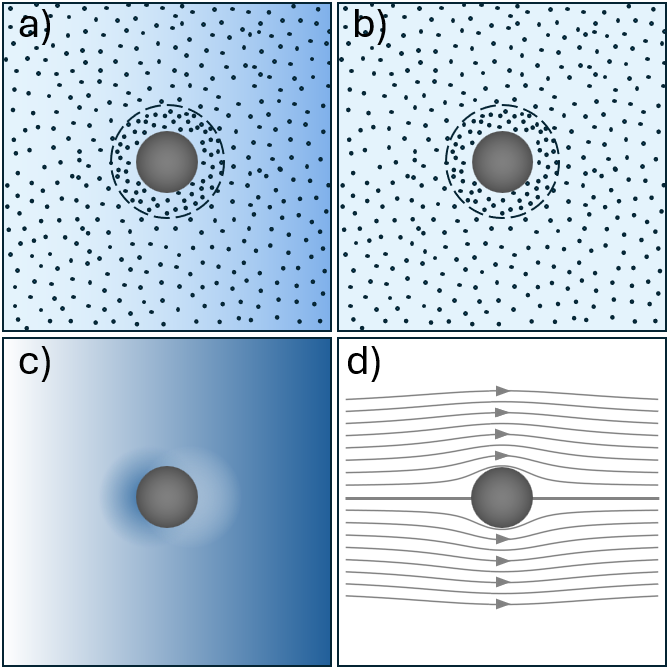
We consider a single colloid of volume $V_{c}$, occupying a region $\nu_{c}$ in the middle of a representative region $\mathcal{V}$, and surrounded by a continuous fluid medium consisting of a viscous microphase only (Fig. 2a). For such a fluid, we simply have $n_{\text{eq},i}^{b}=n_{\text{eq},i}^{r}$. Within $\mathcal{V}$, which is assumed at RLTE (Fig. 2b), we denote the partial region occupied by the fluid by $\tilde{\nu}_{c}$, such that $\mathcal{V}=\tilde{\nu}_{c}\cup\nu_{c}$. Although we assume torques to be absent, the following application of the Lorentz reciprocal theorem may be extended to account for rotational motion based on similar considerations. This has indeed already been accomplished for electrophoresis, but only under the simplifying assumption that no hydrostatic forces are induced around the colloid.[38]

Figure 2: Schematic representation of the reciprocal approach to colloidal motion. a) A single colloid subjected to non-equilibrium forces. The continuum fields that these forces derive from are depicted by a blue background gradient. The dashed circle around the colloid represents the effective boundary between its interfacial region and the bulk fluid. Instead of resolving the local dynamics of a), the reciprocal approach considers two separate auxiliary problems: b) An equilibrium-statistical problem to determine local component distributions, and a continuum-mechanical problem to independently compute c) the non-equilibrium forces and d) the induced Stokes flow field. A stronger background gradient is used in c) to show that the colloid may modify the continuum fields in its vicinity if the transport properties of its solid microphase differ from those of the viscous microphase.

In view of Eq. (23), the momentum continuity equation given by Eq. (13) decouples into two separate continuity equations, one for the forces induced by the colloid, and one for the forces acting on the bulk fluid:

$$\bm{\mathcal{F}}_{\delta}+\nabla\cdot\bm{\sigma}_{\delta}=0,$$ (25)

$$\bm{\mathcal{F}}_{b}+\nabla\cdot\bm{\sigma}_{b}=0,$$ (26)

where $\bm{\sigma}_{\delta}$ and $\bm{\sigma}_{b}$ are the corresponding hydrodynamic stress tensors. The flow velocity can be decomposed accordingly, such that

$$\bm{u}=\bm{u}_{\delta}+\bm{u}_{b},$$ (27)

where $\bm{u}_{b}$ is the bulk fluid flow velocity, and $\bm{u}_{\delta}$ is the induced flow velocity. Similarly, the velocity $\bm{v}$ of the colloid, which we seek to determine, can be expressed as the sum of an induced contribution $\bm{v}_{\Delta}$ and a bulk contribution $\bm{v}_{B}$:

$$\bm{v}=\bm{v}_{\Delta}+\bm{v}_{B},$$ (28)

where each contribution is governed by the forces of the corresponding momentum continuity equation. As the colloidal velocity is not a local continuum field, uppercase subscripts have instead been used in Eq. (28) to avoid confusion.

The momentum continuity equation of the bulk fluid given by Eq. (26) depends on the boundary conditions on $\mathcal{V}$, but is independent of the interfacial boundary conditions at the surface of the colloid. The hydrodynamic stress tensor $\bm{\sigma}_{b}$ of a viscous bulk fluid has the isotropic form

$$\bm{\sigma}_{b}=-P_{db}\bm{I}+\eta\bm{e}_{b},$$ (29)

where $P_{db}$ is the hydrodynamic pressure of the bulk fluid and $\bm{e}_{b}$ is the corresponding strain rate tensor of the bulk fluid flow velocity $\bm{u}_{b}$. As a continuous bulk fluid is electroneutral everywhere ($\omega_{b}=0$), Eq. (16) yields the following forms for the induced thermodynamic force density and bulk force density of the fluid:

$$\bm{\mathcal{F}}_{\delta}=\rho_{\delta}\bm{g}+\omega_{\delta}\bm{E}-\nabla\Pi_{\delta}-\nabla p_{\delta},$$ (30)

$$\bm{\mathcal{F}}_{b}=\rho_{b}\bm{g}-\nabla\Pi_{b}-\nabla p_{b}.$$ (31)

Substituting Eq. (31) into Eq. (26), we can thus write the momentum continuity equation of the bulk fluid as

$$\rho_{b}\bm{g}-\nabla\Pi_{b}-\nabla p_{b}+\nabla\cdot\bm{\sigma}_{b}=0,$$ (32)

where $\Pi_{b}$ is the osmotic pressure of the bulk fluid, $p_{b}$ is the bulk hydrostatic pressure of the solvent reservoir. Since the fluid consists only of a viscous microphase, $\Pi_{b}$ corresponds to the osmotic pressure of the solutes in the bulk fluid. The bulk fluid flow velocity $\bm{u}_{b}$ is then determined by Eqs. (29) and (32).

At RLTE, it is reasonable to consider the limit where the boundaries of $\mathcal{V}$ tend to infinity around the colloid,[24] so that the fluid components form a thermodynamic reservoir. In this limit, the thermodynamic forces induced by a colloid satisfy a ”force-free” balance, corresponding to a generalized Gibbs adsorption equation.[17] The induced solvent reservoir response via $\nabla p_{\delta}$ can only balance those hydrostatic forces in the fluid that do not drive colloidal motion, like the ones induced by a spherically symmetric, chemically active Janus particle.[16, 10] Therefore, the hydrostatic pressure induced in the solvent reservoir exerts no net force on the colloid, such that $\oint_{\partial\nu_{c}}p_{\delta}\bm{n}dS=0$. Noting that $p_{\delta}=p_{\text{ex}}$ because $p$ is only non-zero inside the fluid, this condition can also be expressed as

$$\oint_{\partial\nu_{c}}p_{\text{ex}}\bm{n}dS=0.$$ (33)

Based on Eqs. (11), (18) and (33), the force-free balance equation thus takes the form of a vanishing volume integral over $\mathcal{V}$ of the induced osmotic pressure, such that $\int_{\mathcal{V}}\nabla\Pi_{\delta}d^{3}\bm{r}=0$. Furthermore, overall electroneutrality of $\mathcal{V}$ implies that the volume integrals over $\mathcal{V}$ of the induced electric charge density and the corresponding electric force must also vanish, such that $\int_{\mathcal{V}}\omega_{\delta}d^{3}\bm{r}=0$ and $\int_{\mathcal{V}}\omega_{\delta}\bm{E}d^{3}\bm{r}=0$. These balance equations can instead be expressed in terms of volume integrals over the partial regions occupied by the colloid and the fluid, yielding

$$\int_{\nu_{c}}\nabla\Pi_{c}d^{3}\bm{r}=-\int_{\tilde{\nu}_{c}}\nabla\Pi_{\text{ex}}d^{3}\bm{r},$$ (34)

$$\int_{\nu_{c}}\omega_{c}\bm{E}d^{3}\bm{r}=-\int_{\tilde{\nu}_{c}}\omega_{\text{ex}}\bm{E}d^{3}\bm{r}.$$ (35)

The balance equations given by Eqs. (34) and (35) constitute the prerequisite for force-free motion of a single colloid, as encountered in electro-, diffusio-, and thermophoresis.[3] At RLTE, the fluid excess osmotic pressure gradient $\nabla\Pi_{\text{ex}}=\left.\partial\Pi_{\text{ex}}/\partial\bm{r}\right|_{\left\{\phi_{j}\right\}}$ is evaluated at constant interfacial interaction potentials and related to thermodynamic excess quantities of the local osmotic equation of state via Eq. (18):

$$\nabla\Pi_{\text{ex}}=h_{\text{eq}}^{\text{ex}}\frac{\nabla T}{T}+h_{\text{eq}}^{b}\frac{\nabla T_{\text{ex}}}{T}+\sum_{i}\left(n_{\text{eq},i}^{\text{ex}}\nabla_{T}\mu_{i}+n_{\text{eq},i}^{b}\nabla_{T}\mu_{i}^{\text{ex}}\right),$$ (36)

where we have used superscripts ”ex” and ”$b$” instead of subscripts for the equilibrium densities. According to Eq. (36), a fluid excess osmotic pressure gradient can hence arise not only from an interfacial excess of the densities $h_{\text{eq}}$ and $n_{\text{eq},i}$, but also from the induced deviations $\nabla T_{\text{ex}}$ and $\nabla_{T}\mu_{i}^{\text{ex}}$ of the thermodynamic forces from their bulk values, as depicted in Fig. 2c.

The force density $\bm{\mathcal{F}}_{\delta}$ depends on the boundary conditions at the colloidal surface and decays away from the colloid. More specifically, as the colloid can only induce a finite interfacial excess of mass within the fluid, the volume integral $\int_{\mathcal{V}}\rho_{\text{ex}}d^{3}\bm{r}$ must converge, implying that the gravitational force density $\rho_{\delta}\bm{g}$ decays as $1/r^{4}$ or faster from the colloid. Together with Eqs. (34) and (35), this implies that the volume integral of $\bm{\mathcal{F}}_{\delta}$ is convergent, and that the corresponding hydrodynamic stress $\bm{\sigma}_{\delta}$ and flow velocity $\bm{u}_{\delta}$ must decay at least as $1/r^{2}$ and $1/r$, respectively. It is precisely this hydrodynamic decay behavior that allows for a determination of the induced colloidal velocity $\bm{v}_{\Delta}$ based on the Lorentz reciprocal theorem.

5.2 Application of the Lorentz reciprocal theorem to the induced motion of a single colloid

To evidence this, we now determine $\bm{v}_{\Delta}$ by introducing an auxiliary flow problem inside the same region $\mathcal{V}$, whose quantities are denoted by a subscript ”$*$”. In particular, this problem must be chosen such that the same velocity $\bm{v}_{\Delta}$ is induced by a uniform body force $\bm{F}_{*}$ acting on the colloid, corresponding to an auxiliary momentum continuity equation $\bm{f}_{*}+\nabla\cdot\bm{\sigma}_{*}=0$, where $\bm{f}_{*}=\bm{F}_{*}/V_{c}$ inside the colloid and zero elsewhere. In addition, we require that the flow velocity $\bm{u}_{*}$ vanishes in the far-field and respects the condition of incompressibility, such that $\nabla\cdot\bm{u}_{*}=0$. Under kinematic reversibility, both the induced flow velocity $\bm{u}_{*}$ and hydrodynamic stress tensor $\bm{\sigma}_{*}$ must be linear in the velocity $\bm{v}_{\Delta}$, such that[24]

$$\bm{u}_{*}=\bm{U}\cdot\bm{v}_{\Delta},$$ (37)

$$\bm{\sigma}_{*}=\bm{\mathcal{P}}\cdot\bm{v}_{\Delta},$$ (38)

where the Stokes flow tensor $\bm{U}$ and Stokes stress tensor $\bm{\mathcal{P}}$ are symmetric. We therefore have $\bm{F}_{*}=\bm{\xi}\cdot\bm{v}_{\Delta}$, where the Stokes friction tensor $\bm{\xi}$ of the colloid is related to the auxiliary hydrodynamic traction tensor $\bm{\Lambda}=\bm{n}\cdot\bm{\mathcal{P}}$ via $\bm{\xi}=\oint_{\partial\nu_{c}}\bm{n}\cdot\bm{\mathcal{P}}dS=0$. Inside the colloid, the Stokes flow must further satisfy

$$\bm{U}=\bm{I}.$$ (39)

According to the above conditions for the auxiliary Stokes flow, the hydrodynamic stress $\bm{\sigma}_{*}$ and flow velocity $\bm{u}_{*}$ decay as $1/r^{2}$ and $1/r$, respectively.

The thermodynamic forces and hydrodynamic stresses induced by a single colloid thus represent continuum-mechanical fluctuations relative to the bulk fluid. As shown in appendix A, contracting the momentum continuity equation of one flow problem with the velocity field of the other flow problem yields the relation

$$\underbrace{\int_{\mathcal{V}}\bm{u}_{*}\cdot\bm{\mathcal{F}}_{\delta}\,d^{3}\bm{r}}_{I_{1}} -\underbrace{\int_{\mathcal{V}}\bm{u}_{\delta}\cdot\bm{f}_{*}\,d^{3}\bm{r}}_{I_{2}}$$

$$=\underbrace{\int_{\mathcal{V}}\nabla\cdot\left(\bm{u}_{\delta}\cdot\bm{\sigma}_{*}-\bm{u}_{*}\cdot\bm{\sigma}_{\delta}\right)\,d^{3}\bm{r}}_{I_{3}}.$$ (40)

The final form of the Lorentz reciprocal theorem is obtained by applying Gauss’ theorem to the surface integral of the divergence on the right-hand side of Eq. (40).[30] However, this does not directly yield an expression for the velocity $\bm{v}_{\Delta}$. To this end, we must further examine the integrals in Eq. (40) based on the specific conditions satisfied by the considered flows.

Since there is only a non-equilibrium force acting on the colloid in the auxiliary problem, integral $I_{2}$ takes the simple form

$$I_{2}=\bm{v}_{\Delta}\cdot\bm{F}_{*}=\bm{v}_{\Delta}\cdot\bm{\xi}\cdot\bm{v}_{\Delta}.$$ (41)

Integral $I_{1}$ can be re-expressed in terms of volume integrals over the colloid and the fluid. With Eq. (16), the induced thermodynamic force densities inside these regions take the forms $\bm{\mathcal{F}}_{c}=\rho_{c}\bm{g}+\omega_{c}\bm{E}-\nabla\Pi_{c}$ and $\bm{\mathcal{F}}_{\text{ex}}=\rho_{\text{ex}}\bm{g}+\omega_{\text{ex}}\bm{E}-\nabla\Pi_{\text{ex}}-\nabla p_{\text{ex}}$. Using these expressions for $\bm{\mathcal{F}}_{\delta}$ in the respective regions, Eqs. (37) and (39) for the Stokes flow, the force-free conditions given by Eqs. (34) and (35), and Eq. (121), integral $I_{1}$ becomes

$$I_{1} = \bm{v}_{\Delta}\cdot\left[m_{c}\bm{g}+\int_{\tilde{\nu}_{c}}\rho_{\text{ex}}\bm{U}d^{3}\bm{r}\cdot\bm{g}\right.$$ (42)

$$\hskip 12.80365pt+\left.\int_{\tilde{\nu}_{c}}\left(\bm{U}-\bm{I}\right)\cdot\left(\omega_{\text{ex}}\bm{E}-\nabla\Pi_{\text{ex}}\right)d^{3}\bm{r}\right],$$

where $m_{c}=\int_{\nu_{c}}\rho_{c}d^{3}\bm{r}$ is the mass of the colloid.

To make progress with integral $I_{3}$, we use Gauss’ theorem to obtain

$$I_{3} = \oint_{\partial\mathcal{V}}\left(\bm{u}_{\delta}\cdot\bm{\sigma}_{*}-\bm{u}_{*}\cdot\bm{\sigma}_{\delta}\right)\cdot\bm{n}dS$$ (43)

$$-\oint_{\partial\nu_{m}}\left(\bm{v}^{\parallel}_{\delta}\cdot\bm{\sigma}_{*}-\bm{v}^{\parallel}_{*}\cdot\bm{\sigma}_{\delta}\right)\cdot\bm{n}dS.$$

where $\bm{n}$ is the outward-pointing unit normal vector to the closed interfacial boundaries $\partial\nu_{m}$ of all microparticles. The microparticles occupy a region $\nu_{m}=\bigcup_{\lambda}\nu_{\lambda}$ within $\mathcal{V}$, where $\nu_{\lambda}$ is the partial volume of microparticle species $\lambda$. In the present case, the only microparticle inside $\mathcal{V}$ is the colloid, such that $\nu_{m}=\nu_{c}$. The quantities $\bm{v}^{\parallel}_{\delta}$ and $\bm{v}^{\parallel}_{*}$ are the tangential slip velocities at these boundaries in each flow problem. As thermal transpiration is negligible at low Knudsen number,[8] these slip velocities respect the hydrodynamic boundary condition as specified by the general Navier slip formula:[6]

$$\bm{v}^{\parallel}_{\delta}=\bm{u}_{a}+\frac{l_{\text{slip}}}{\eta}\left(\bm{I}-\bm{n}\bm{n}\right)\cdot\left(\bm{n}\cdot\bm{\sigma}_{\delta}\right),$$ (44)

$$\bm{v}^{\parallel}_{*}=\frac{l_{\text{slip}}}{\eta}\left(\bm{I}-\bm{n}\bm{n}\right)\cdot\left(\bm{n}\cdot\bm{\sigma}_{*}\right).$$ (45)

In the actual flow problem, the active slip velocity $\bm{u}_{a}$ at the colloidal surface accounts for a force-free self-propulsion mechanism arising from non-hydrostatic forces within the colloid, as encountered in microswimming.[9] As for dynamic viscosity, the principle of kinematic reversibility justifies the use of the same hydrodynamic slip length $l_{\text{slip}}$ in both flow problems. Let us consider the integral of the term $\bm{v}^{\parallel}_{\delta}\cdot\bm{\sigma}_{*}\cdot\bm{n}$ over the interfaces in Eq. (43). Substituting Eq. (44), we can write $\left(\left(\bm{I}-\bm{n}\bm{n}\right)\cdot\left(\bm{n}\cdot\bm{\sigma}_{\delta}\right)\cdot\bm{\sigma}_{*}\right)\cdot\bm{n}=\left(\bm{n}\cdot\bm{\sigma}_{\delta}\right)\cdot\left(\bm{n}\cdot\bm{\sigma}_{*}\right)-\left(\bm{n}\cdot\bm{\sigma}_{\delta}\cdot\bm{n}\right)\cdot\left(\bm{n}\cdot\bm{\sigma}_{*}\cdot\bm{n}\right)$, which is symmetric in the interchange of $\bm{\sigma}_{\delta}$ and $\bm{\sigma}_{*}$. This symmetry relation between hydrodynamic stresses and flows highlights the necessity of distinguishing hydrodynamic stress from hydrostatic stress. With this symmetry relation and Eq. (38), we therefore get $\oint_{\partial\nu_{m}}\left(\bm{v}^{\parallel}_{\delta}\cdot\bm{\sigma}_{*}-\bm{v}^{\parallel}_{*}\cdot\bm{\sigma}_{\delta}\right)\cdot\bm{n}dS=\bm{v}_{\Delta}\cdot\oint_{\partial\nu_{c}}\left(\bm{\Lambda}\cdot\bm{u}_{a}\right)dS$. Since the terms $\bm{u}_{\delta}\cdot\bm{\sigma}_{*}$ and $\bm{u}_{*}\cdot\bm{\sigma}_{\delta}$ both decay as $1/r^{3}$ or faster from the colloid, their surface integrals over $\partial\mathcal{V}$ vanish, such that $\oint_{\partial\mathcal{V}}\bm{u}_{\delta}\cdot\bm{\sigma}_{*}\cdot\bm{n}dS=0$ and $\oint_{\partial\mathcal{V}}\bm{u}_{*}\cdot\bm{\sigma}_{\delta}\cdot\bm{n}dS=0$. Combining the above relations, integral $I_{3}$ thus reduces to

$$I_{3}=-\bm{v}_{\Delta}\cdot\oint_{\partial\nu_{c}}\left(\bm{\Lambda}\cdot\bm{u}_{a}\right)dS.$$ (46)

Substitution of Eqs. (42), (41) and (46) into Eq. (40) finally yields the balance equation

$$m_{c}\bm{g}+\int_{\tilde{\nu}_{c}}\rho_{\text{ex}}\bm{U}d^{3}\bm{r}\cdot\bm{g} + \int_{\tilde{\nu}_{c}}\left(\bm{U}-\bm{I}\right)\cdot\left(\omega_{\text{ex}}\bm{E}-\nabla\Pi_{\text{ex}}\right)d^{3}\bm{r}$$ (47)

$$- \bm{\xi}\cdot\bm{v}_{\Delta}+\oint_{\partial\nu_{c}}\left(\bm{\Lambda}\cdot\bm{u}_{a}\right)dS=0.$$

The expression of the induced colloidal velocity $\bm{v}_{\Delta}$ can now be obtained by rearrangement of Eq. (47), giving

$$\bm{v}_{\Delta} = \frac{1}{\bm{\xi}}\cdot\left(m_{c}\bm{I}+\int_{\tilde{\nu}_{c}}\rho_{\text{ex}}\bm{U}d^{3}\bm{r}\right)\cdot\bm{g}$$ (50)

$$+\frac{1}{\bm{\xi}}\cdot\int_{\tilde{\nu}_{c}}\left(\bm{U}-\bm{I}\right)\cdot\left(\omega_{\text{ex}}\bm{E}-\nabla\Pi_{\text{ex}}\right)d^{3}\bm{r}$$

$$+\frac{1}{\bm{\xi}}\cdot\oint_{\partial\nu_{c}}\left(\bm{\Lambda}\cdot\bm{u}_{a}\right)dS.$$

Notably, this expression of $\bm{v}_{\Delta}$ only refers to the hydrodynamic tensors $\bm{U}$ and $\bm{\Lambda}$ of the auxiliary Stokes problem, which are well established.[4] The Stokes flow tensor $\bm{U}$ in the fluid region accounts for the hydrodynamic drag on the colloid due to thermodynamic forces in the fluid. This drag vanishes when the colloid’s hydrodynamic radius tends to zero ($\bm{U}=0$), which is also known as the Hückel limit.[32] Hence, the term relating to $\rho_{\text{ex}}$ in Eq. (50) is due to the hydrodynamic drag exerted on the colloid due to local fluid flows induced by the interfacial excess weight of fluid around it. Due to the uniformity of the gravitational field $\bm{g}$, the Onsager-like symmetry of this term is already apparent: the colloidal velocity $\int_{\tilde{\nu}_{c}}\rho_{\text{ex}}\bm{U}d^{3}\bm{r}\cdot\bm{g}/\bm{\xi}$ induced by the fluid excess weight is the same as the flow of fluid excess mass induced by a body force on the colloid.

The terms in Eqs (50) and (50) represent force-free colloidal motion. The term in Eq. (50) represents active swimming due to a prescribed slip velocity on the colloid’s surface. The term in Eq. (50) corresponds to the velocity due to electro-, diffusio-, or thermophoresis,[17] also describing the active motion of a self-diffusiophoretic or self-thermophoretic colloid to first order in the thermodynamic forces.[16] The contraction between the phoretic force density $\omega_{\text{ex}}\bm{E}-\nabla\Pi_{\text{ex}}$ and the flow tensor $\bm{U}-\bm{I}$, which describes the auxiliary Stokes flow in the rest frame of the colloid (Fig. 2d), thus contributes to a colloidal velocity in the direction opposite to the phoretic force density. This prediction is consistent with the force-free nature of phoretic motion: fluid flows in the direction of the phoretic force density, whereas the colloid is pushed in the opposite direction. For (self-)diffusio- or thermophoresis, Eq. (50) also shows that the colloid is pushed towards regions of higher excess osmotic pressure $\Pi_{\text{ex}}$ within the fluid. This conclusion refutes the ”osmotic motor” model, which predicts phoretic motion to lower excess osmotic pressure.[19] For diffusiophoresis at high dilution, a recent attempt[11] to recover this model from an expression similar to Eq. (50) was made based on the model’s underlying assumption that the excess fluid exerts a net hydrostatic pressure force of $-\oint_{\partial\nu_{c}}\Pi_{\text{ex}}\bm{n}dS$ on the colloid, which, however, breaks the widely accepted force-free condition.[25]

As shown in Appendix B, the bulk contribution $\bm{v}_{B}$ to the colloid’s velocity can be determined directly from the actual flow problem using well developed methods, yielding

$$\bm{v}_{B}=-\frac{1}{\bm{\xi}}\cdot\int_{\nu_{c}}\left(\nabla\Pi_{b}+\nabla p_{b}\right)d^{3}\bm{r}+\left.\bm{u}_{b}\right|_{\bm{r}_{c}}+\left.\bm{\mathcal{M}}\left[\bm{u}_{b}\right]\right|_{\bm{r}_{c}},$$ (51)

where $\bm{\mathcal{M}}$ is a shape-dependent integro-differential operator acting on the bulk fluid flow velocity $\bm{u}_{b}$, evaluated at the colloid’s hydrodynamic center $\bm{r}_{c}$. Using Eq. (51) and Eqs. (50)-(50) in Eq. (28), the expression of the total velocity $\bm{v}$ of the colloid finally becomes

$$\bm{v} = \frac{1}{\bm{\xi}}\cdot\left(m_{c}\bm{I}+\int_{\tilde{\nu}_{c}}\rho_{\text{ex}}\bm{U}d^{3}\bm{r}\right)\cdot\bm{g}$$

$$+\frac{1}{\bm{\xi}}\cdot\int_{\tilde{\nu}_{c}}\left(\bm{U}-\bm{I}\right)\cdot\left(\omega_{\text{ex}}\bm{E}-\nabla\Pi_{\text{ex}}\right)d^{3}\bm{r}$$

$$+\frac{1}{\bm{\xi}}\cdot\oint_{\partial\nu_{c}}\left(\bm{\Lambda}\cdot\bm{u}_{a}\right)dS$$

$$-\frac{1}{\bm{\xi}}\cdot\int_{\nu_{c}}\left(\nabla\Pi_{b}+\nabla p_{b}\right)d^{3}\bm{r}+\left.\bm{u}_{b}\right|_{\bm{r}_{c}}+\left.\bm{\mathcal{M}}\left[\bm{u}_{b}\right]\right|_{\bm{r}_{c}}.$$

Eq. (LABEL:eq:-46) describes the translational velocity of a single colloid under any transport mechanism to first order in the non-equilibrium forces and is the main result of this section.

5.3 Discussion of results and boundary conditions

Our result for force-free phoretic motion given by Eq. (50) is consistent with the result previously obtained from an Onsager reciprocal,[17] which has been used to generalize the Henry function for electrophoresis and the Ruckenstein function for thermophoresis to arbitrary hydrodynamic boundary conditions and interfacial layer thicknesses. Furthermore, this expression has been shown to align with mesoscale-molecular simulations[13] and successfully describes experimental measurements on thermophoresis of DNA without any free fitting parameters.[15] However, this approach did not account for active swimming and only considered diffusive motion at hydrostatic equilibrium, without elucidating the role of the solvent reservoir in momentum relaxation under different boundary conditions.

If the colloid and fluid are contained within a large closed box, then flow is prohibited in the bulk fluid, which must hence remain at hydrostatic equilibrium. In this case, $\bm{u}_{b}=0$ and $\bm{\sigma}_{b}=0$, so that Eq. (32) reduces to

$$\rho_{b}\bm{g}-\nabla\Pi_{b}-\nabla p_{b}=0,$$ (53)

which fixes the bulk hydrostatic pressure gradient $\nabla p_{b}$ of the solvent reservoir. Noting that the mass density $\rho_{b}$ of a continuous bulk fluid is uniform at RLTE, Eq. (126) then reduces to

$$\bm{v}_{B}=-\frac{\bm{g}}{\bm{\xi}}\int_{\nu_{c}}\rho_{b}d^{3}\bm{r}=-\frac{1}{\bm{\xi}}V_{c}\rho_{b}\bm{g},$$ (54)

where $V_{c}\rho_{b}$ represents the mass of bulk fluid displaced by the colloid, giving rise to buoyancy. Conversely, if the colloid and fluid are confined to a narrow, open pipe whose ends are kept at the same solvent reservoir pressure, then momentum is instead dissipated through viscous shear and buoyancy is absent. In this case, $\nabla p_{b}=0$ and Eq. (126) becomes

$$\bm{v}_{B}=-\frac{1}{\bm{\xi}}\cdot\int_{\nu_{c}}\nabla\Pi_{b}d^{3}\bm{r}+\left.\bm{u}_{b}\right|_{\bm{r}_{c}}+\bm{\mathcal{M}}\left[\bm{u}_{b}\right]_{\bm{r}_{c}},$$ (55)

where, in view of Eqs. (32), the bulk fluid flow velocity $\bm{u}_{b}$ is now determined by

$$\rho_{b}\bm{g}-\nabla\Pi_{b}+\nabla\cdot\bm{\sigma}_{b}=0.$$ (56)

The first term in Eq. (55) shows that, unlike the excess fluid, the bulk fluid can exert a net hydrostatic pressure force $-\oint_{\partial\nu_{c}}\Pi_{b}\bm{n}dS$ on the colloid, but only under open system boundary conditions that give way to a hydrodynamic rather than hydrostatic response of the solvent reservoir. Under these conditions, it can then also be seen from Eq. (56) that the gradient $\nabla\Pi_{b}$ acts as a driving force of flow, alongside the gravitational force density $\rho_{b}\bm{g}$ of the bulk fluid.

To further verify and analyze our results, we consider a spherically symmetric colloid of hydrodynamic radius $R$. The hydrodynamic tensors are then given by

$$\bm{\xi}=6\pi a\eta R\bm{I},$$ (57)

$$\bm{\mathcal{M}}=\frac{R^{2}}{6}\nabla^{2},$$ (58)

$$\bm{\Lambda}=\frac{3a\eta}{2R}\left(\hat{\bm{r}}\hat{\bm{r}}-\bm{I}\right),$$ (59)

$$\bm{U}=\frac{3R}{4r}\left(a\left(\mathbf{I}+\hat{\mathbf{r}}\hat{\mathbf{r}}\right)-\left(a-\frac{2}{3}\right)\frac{R^{2}}{r^{2}}\left(3\hat{\mathbf{r}}\hat{\mathbf{r}}-\mathbf{I}\right)\right),$$ (60)

where $\hat{\bm{r}}$ is the outward-pointing radial unit vector. The slip coefficient $a=(1+2l_{\text{slip}}/R)/(1+3l_{\text{slip}}/R)$ takes the value $1$ for a non-slip boundary condition and $2/3$ for a perfect-slip boundary condition. With Eqs. (57) and (59), the contribution due to active swimming then takes the familiar form[37]

$$\frac{1}{\bm{\xi}}\cdot\oint_{\partial\nu_{c}}\left(\bm{\Lambda}\cdot\bm{u}_{a}\right)dS=-\frac{1}{4\pi R^{2}}\cdot\oint_{\partial\nu_{c}}\bm{u}_{a}dS.$$ (61)

To the best of our knowledge, the contribution due to the fluid excess weight in Eq. (50) has attracted little to no attention in literature so far. Although this contribution is generally expected to be weak compared to other transport mechanisms, it might be relevant when density-matched colloids are sedimenting under gravity. The force required to keep such a colloid at rest is then $-\bm{m}\bm{g}$, where the cross-coupling mass tensor is given by $\bm{m}=\int_{\tilde{\nu}_{c}}\rho_{\text{ex}}\bm{U}d^{3}\bm{r}$. A particularly simple expression of $\bm{m}$ is obtained in the boundary layer approximation, where we have $\bm{m}=m_{\text{ex}}\left\langle\bm{U}\right\rangle_{\partial\nu_{c}}$, where $\left\langle\bm{U}\right\rangle_{\partial\nu_{c}}$ is the average of $\bm{U}$ over the colloidal surface and $m_{\text{ex}}=\int_{\tilde{\nu}_{c}}\rho_{\text{ex}}d^{3}\bm{r}$ is the fluid excess mass around the colloid. Since Eq. (60) gives $\left\langle\bm{U}\right\rangle_{\partial\nu_{c}}=a\bm{I}$, we obtain

$$\bm{m}=am_{\text{ex}}\bm{I}.$$ (62)

In the boundary layer approximation, $\bm{m}$ thus scales with the slip parameter $a$ and the fluid excess mass. Given that the friction coefficient $\bm{\xi}$ of the colloid also scales with $a$, this implies that the corresponding contribution $\int_{\tilde{\nu}_{c}}\rho_{\text{ex}}\bm{U}d^{3}\bm{r}\cdot\bm{g}/\bm{\xi}$ to its velocity is independent of the hydrodynamic boundary condition at its surface.

In addition, our framework predicts a novel contribution to phoretic motion that cannot be derived from interfacial thermodynamics, since it stems from thermodynamic force fluctuations when interfacial excess is absent. To evidence this, we consider a fluid at constant temperature, containing a single neutral solute component $k$ with an ideal-gas equation of state. The osmotic pressure gradient inside the fluid is then given by $\nabla\Pi=k_{B}T\nabla n_{k}^{r}$. For diffusiophoretic motion, we assume that a constant gradient $\nabla n_{k}^{b}$ in solute number density is maintained in the bulk, so that its reservoir gradient $\nabla n_{k}^{r}$ tends to $\nabla n_{k}^{b}$ far away from the colloid. The diffusion flux of an ideal solute must take the form $\bm{j}_{k}=-L_{kk}\nabla_{T}\mu_{k}$, where $\nabla_{T}\mu_{k}=k_{B}T\nabla\ln n_{k}^{r}$ and $k_{B}$ is the Boltzmann constant. As the corresponding equilibrium density $n_{\text{eq},k}=n_{\text{eq},i}^{b}$ is uniform inside the fluid when interfacial potential interactions are absent, the same must be true for the Onsager coefficient $L_{kk}$. With vanishing normal component of $j_{k}$ and no reaction at the colloidal surface, solving $\nabla\cdot\bm{j}_{k}=0$ then yields the following form of the osmotic pressure gradient inside the fluid:

$$\nabla\Pi=\left(\bm{I}-\frac{R^{3}}{2r^{3}}\left(3\hat{\bm{r}}\hat{\bm{r}}-\bm{I}\right)\right)\cdot\nabla\Pi_{b},$$ (63)

where $\nabla\Pi_{b}=k_{B}T\nabla n_{k}^{b}$. In the absence of gravity and active swimming, the induced colloidal velocity reduces to $\bm{v}_{\Delta}=-\int_{\tilde{\nu}_{c}}\left(\bm{U}-\bm{I}\right)\cdot\nabla\Pi_{\text{ex}}d^{3}\bm{r}/\xi$, where $\Pi_{\text{ex}}=\Pi-\Pi_{b}$. Using Eqs. (57), (60) and (63), we thus obtain

$$\bm{v}_{\Delta}=\frac{R^{2}k_{B}T}{9a\eta}\nabla n_{k}^{b},$$ (64)

which can give diffusiophoretic speeds of $\sim 0.1-1\,\mu\text{m/s}$ based on typical parameter values. Eq. (64) predicts diffusiophoresis towards higher bulk solute concentration. This behavior can be understood intuitively: As the solute cannot diffuse through the colloid, it will accumulate on the side of the colloid facing the bulk solute flux and deplete from the other side. This diffusive polarization induces an excess osmotic pressure gradient, and subsequently a flow, towards lower bulk solute concentration, which means that the colloid will be drawn towards higher bulk solute concentration.

Moreover, if the gradient $\nabla n_{k}^{b}$ is maintained within a long cylindrical pipe that opens into the same solvent reservoir at constant pressure on either side, then Eq. (56) yields the Poiseuille profile $\bm{u}_{b}=-k_{B}T\left(R_{p}^{2}-y^{2}\right)\nabla n_{k}^{b}/\left(4\eta\right)$ for the bulk fluid flow velocity, where $y$ is the radial distance from the central axis and $R_{p}$ is the pipe radius. With Eq. (58), the bulk velocity of the colloid given by Eq. (55) becomes

$$\bm{v}_{B}=\left(-\frac{2}{9a}+\frac{1}{6}-\frac{R_{p}^{2}}{4R^{2}}\left(1-\frac{y^{2}}{R_{p}^{2}}\right)\right)\frac{R^{2}k_{B}T}{\eta}\nabla n_{k}^{b}.$$ (65)

For $R_{p}/R\gg 1$, the advective transport due to bulk flow thus dominates over the contributions from the Faxén correction and the bulk osmotic pressure.

To conclude this section, we note that Eq. (LABEL:eq:-46) has been derived under the assumption that the fluid consists of a viscous microphase only. Determining the motion of a single colloid becomes challenging when the fluid contains other microparticles, which turn the dynamics into a many-body interaction problem. Moreover, we have not accounted for thermal fluctuations, which can in principle be modeled separately by adding a stochastic Brownian contribution to Eq. (28) that respects a fluctuation-dissipation relation.[23] In view of the challenges posed by many-body interactions, it is worth noting that many industrial applications are not concerned with the motion of each individual colloid. Instead, the relevant dynamics can often be captured by an ensemble-averaged description, especially in colloidal suspensions where fluctuations and many-body effects may either average out or be represented by continuum-statistical driving forces. The remainder of this paper will therefore focus on developing such a continuum-statistical description of colloidal dynamics under the assumption of kinematic reversibility.

6 Continuum-statistical colloidal dynamics

6.1 Macroscopic continuity equations

Our goal is to close the particle number continuity equation, as given by Eq. (3), for the determination of the colloidal number density. However, colloids are identical microparticles composed of the same solid microphase. The volume of a single colloid thus exceeds the continuum scale set by $dV$, rendering the colloidal number density a discontinuous distribution function at the continuum scale.

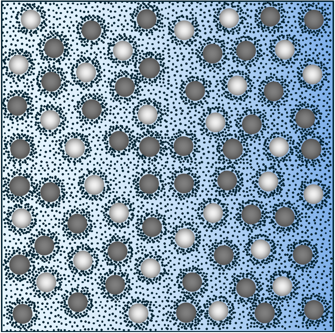
A continuum-statistical description of colloidal motion therefore relies on the recovery of the continuity equations at the macroscale, which requires the suspension to be statistically homogeneous and isotropic (Fig. 3).[10] These macroscopic continuity equations are used to study the evolution of mean-fields, which also set the boundary conditions on representative volume elements for the local steady-states governed by Eqs. (5), (6) and (17). Homogeneity and isotropy are generally justified in the bulk of a suspension if the microparticles are randomly dispersed. However, these conditions may break down for highly active colloids over longer timescales, when strong alignment and clustering can occur due to spatial correlations in orientation resulting from a coupling between active stresses and thermal fluctuations.[27] The following continuum-statistical development will therefore be restricted to translational motion where active swimming is absent and where chemical or thermal activity do not induce such correlations.

Figure 3: A representative volume element of a homogeneous, isotropic suspension. The blue background gradient shows that the volume element is subjected to forces due to non-equilibrium boundary conditions.

To homogenize the suspension, we divide it into a fixed mesh of macroscopic representative volume elements of size $V$ and consider a local continuum field denoted by $\bm{q}$. Within a volume element $\mathcal{V}$, let $\nu_{\alpha}$ denote the partial region of volume $V_{\alpha}$ occupied by a given medium $\alpha$, which may or may not be continuous. If the medium is statistically homogeneous over $\mathcal{V}$, then the ensemble average of $\bm{q}$ over that medium inside $\mathcal{V}$ is equal to the volume average over its partial region $\nu_{\alpha}$.[10] We can therefore introduce the partial mean-field of $\bm{q}$ over the medium as

$$\left\langle\bm{q}\right\rangle_{\nu_{\alpha}}=\frac{1}{V_{\alpha}}\int_{\nu_{\alpha}}\bm{q}d^{3}\bm{r}.$$ (66)

Now consider an elementary volume $dV$ at position $\bm{r}$ inside $\mathcal{V}$. We define the partial mean-field of $\bm{q}$ at $\bm{r}$ as the volume average over a partial region $\nu_{\alpha}(\bm{r})$ of volume $V_{\alpha}$ centered around $\bm{r}$, which allows us to describe its local spatial variations via $\left\langle\bm{q}\right\rangle_{\nu_{\alpha}(\bm{r})}$. To leading order in the forces, we can write $\left\langle\bm{q}\right\rangle_{\nu_{\alpha}(\bm{r})}=\left\langle\bm{q}\right\rangle_{\nu_{\alpha}}$ and $\nabla\left\langle\bm{q}\right\rangle_{\nu_{\alpha}(\bm{r})}=\bar{\nabla}\left\langle\bm{q}\right\rangle_{\nu_{\alpha}}$, where $\bar{\nabla}$ denotes the macroscopic gradient defined over adjacent volume elements. For the same volume element, we define the local fluctuation of $\bm{q}$ inside $\nu_{\alpha}$ as

$$\bm{q}^{\prime}_{\nu_{\alpha}}=\bm{q}-\left\langle\bm{q}\right\rangle_{\nu_{\alpha}},$$ (67)

such that $\left\langle\bm{q}^{\prime}_{\nu_{\alpha}}\right\rangle_{\nu_{\alpha}}=0$. Moreover, if $\bm{q}$ is the flux of a conserved quantity, then the ensemble-averaged divergence of $\bm{q}$ over a homogeneous and isotropic medium is equal to the divergence of its partial mean-field:[10]

$$\left\langle\nabla\cdot\bm{q}\right\rangle_{\nu_{\alpha}}=\bar{\nabla}\cdot\left\langle\bm{q}\right\rangle_{\nu_{\alpha}}.$$ (68)

If the suspension is homogeneous and isotropic, then Eqs. (66) to (68) apply to the entire volume element $\mathcal{V}$ and we simply write

$$\left\langle\bm{q}\right\rangle_{\mathcal{V}}=\left\langle\bm{q}\right\rangle,$$ (69)

where $\left\langle\bm{q}\right\rangle$ is the suspension mean-field of $\bm{q}$. This mean-field can further be expressed as a weighted sum of partial mean-fields. In terms of the partial region $\nu_{\alpha}$ of a given medium, we have

$$\left\langle\bm{q}\right\rangle=\gamma_{\alpha}\left\langle\bm{q}\right\rangle_{\nu_{\alpha}}+\tilde{\gamma}_{\alpha}\left\langle\bm{q}\right\rangle_{\tilde{\nu}_{\alpha}},$$ (70)

where $\gamma_{\alpha}=V_{\alpha}/V$ is the corresponding volume fraction and $\tilde{\nu}_{\alpha}=\mathcal{V}\setminus\nu_{\alpha}$ represents the remaining region, such that $\tilde{\gamma}_{\alpha}=1-\gamma_{\alpha}=(V-V_{\alpha})/V$.

Homogenization thus enables an ensemble-averaged description that coincides with volume averaging over a macroscopic volume element. Fluctuations that do not influence the average dynamics vanish upon averaging, whereas those that do contribute manifest as continuum-mechanical deviations from the mean-field behavior. Taking the averages of Eqs. (6) and (3) over $\mathcal{V}$, and using Eq. (68), the macroscopic continuity equation for energy and particle number can respectively be written as

$$\bar{\nabla}\cdot\left\langle\bm{j}_{q}\right\rangle=\left\langle Q\right\rangle,$$ (71)

and

$$\frac{\partial\left\langle n_{i}^{r}\right\rangle}{\partial t}+\bar{\nabla}\cdot\left\langle\bm{J}_{i}\right\rangle=\left\langle\Gamma_{i}\right\rangle.$$ (72)

As we have shown, the motion of a single colloid naturally decomposes into induced contributions and contributions from the bulk. To describe the dynamics of colloids continuum-statistically, however, we must consider not only the bulk fluid, but the entire bulk of the suspension, including all microparticles. To this end, we decompose the flow inside the suspension into a mean flow and a diffusive flow, such that $\bm{u}=\left\langle\bm{u}\right\rangle+\bm{u}^{\prime}$, where $\left\langle\bm{u}\right\rangle$ is the mean flow velocity, or advective velocity, of the suspension.[5] The diffusion flow velocity $\bm{u}^{\prime}$ represents the flow velocity inside the inertial reference frame of zero mean volume flux, such that

$$\left\langle\bm{u}^{\prime}\right\rangle=0.$$ (73)

Averaging Eq. (2) over $\mathcal{V}$, and using Eq. (68), we get

$$\bar{\nabla}\cdot\left\langle\bm{u}\right\rangle=0,$$ (74)

which also implies $\nabla\cdot\bm{u}^{\prime}=0$, so that both the advective flow and diffusion flow are incompressible. The particle flux of component $i$ now takes the form

$$\bm{J}_{i}=n_{i}^{r}\left\langle\bm{u}\right\rangle+n_{i}^{r}\bm{u}^{\prime}+\bm{j}_{i},$$ (75)

so that the corresponding mean particle flux $\left\langle\bm{J}_{i}\right\rangle$ becomes

$$\left\langle\bm{J}_{i}\right\rangle=\left\langle n_{i}^{r}\right\rangle\left\langle\bm{u}\right\rangle+\bm{\mathcal{J}}_{i}$$ (76)

where

$$\bm{\mathcal{J}}_{i}=\left\langle n_{i}^{r}\bm{u}^{\prime}\right\rangle+\left\langle\bm{j}_{i}\right\rangle$$ (77)

is the mean diffusion flux and $\left\langle n_{i}^{r}\bm{u}^{\prime}\right\rangle$ is the mean diffusion flow of component $i$.

To introduce the macroscopic colloidal component, we can consider any given species $\lambda$ of microparticles inside the suspension, such that $N_{\lambda}$ identical colloids, each of size $V_{\lambda}$, occupy a partial region $\nu_{\lambda}$ of a volume element $\mathcal{V}$. The fluid surrounding these colloids thus occupies a partial region $\tilde{\nu}_{\lambda}=\mathcal{V}\setminus\nu_{\lambda}$ and may also comprise other species of microparticles. The volume fractions of the colloids and the fluid are denoted by $\gamma_{\lambda}$ and $\tilde{\gamma}_{\lambda}$, respectively, such that $\gamma_{\lambda}=NV_{\lambda}/V$ and $\tilde{\gamma}_{\lambda}=1-\gamma_{\lambda}$. As shown in appendix C, the colloidal continuity equation can be expressed as

$$\frac{\partial c_{\lambda}}{\partial t}+\left\langle\bm{u}\right\rangle\cdot\bar{\nabla}c_{\lambda}+\bar{\nabla}\cdot\bm{\mathcal{J}}_{\lambda}=\Gamma_{\lambda},$$ (78)

where $c_{\lambda}$ is the colloidal number density, $\Gamma_{\lambda}$ is the corresponding chemical source density and $\bm{\mathcal{J}}_{\lambda}=\left\langle n_{\lambda}\bm{u}^{\prime}\right\rangle$ is the colloidal diffusion flux. Moreover, the corresponding diffusion velocity $\bm{v}_{\lambda}$ can be introduced via $\bm{\mathcal{J}}_{\lambda}=c_{\lambda}\bm{v}_{\lambda}$. In appendix C, we also show that the mean diffusion flow of a solute or solvent component $i$ can be expressed in terms of the colloidal diffusion fluxes, yielding the macroscopic particle number continuity equation

$$\frac{\partial\left\langle n_{i}^{r}\right\rangle}{\partial t} +\left\langle\bm{u}\right\rangle\cdot\bar{\nabla}\left\langle n_{i}^{r}\right\rangle$$ (79)

$$-\bar{\nabla}\cdot\left(\bar{V}_{m}\left\langle n_{\text{eq},i}^{r}\right\rangle_{\nu_{\eta}}\sum_{\lambda}\bm{\mathcal{J}}_{\lambda}\right)+\bar{\nabla}\cdot\left\langle\bm{j}_{i}\right\rangle=\left\langle\Gamma_{i}\right\rangle,$$ (80)

where $\bar{V}_{m}=V_{m}/\sum_{\lambda}N_{\lambda}$ is the average volume of a microparticle. $\nu_{\eta}$ denotes the partial region of the viscous microphase inside $\mathcal{V}$, such that $\mathcal{V}=\nu_{\eta}\cup\nu_{m}$, where $\nu_{m}$ is the partial region of volume $V_{m}$ occupied by all microparticles.

Evidently, solving the macroscopic particle number continuity equations governed by Eqs. (72) and (78) requires closed forms of the advective velocity $\left\langle\bm{u}\right\rangle$ and the colloidal diffusion flux $\bm{\mathcal{J}}_{\lambda}$. To determine these forms, we must consider the mean-field and fluctuation of the local momentum continuity equation in a homogeneous, isotropic suspension. As shown in appendix D, the macroscopic momentum balance equation takes the form

$$\left\langle\rho\right\rangle\bm{g}-\left\langle\nabla\Pi\right\rangle-\left(1-\gamma_{m}\right)\bar{\nabla}\bar{p}+\bar{\nabla}\cdot\left\langle\bm{\sigma}_{d}\right\rangle=0,$$ (81)

where $\gamma_{m}=1-\gamma_{\eta}$ is the microparticle volume fraction and $\bar{p}=\left\langle p\right\rangle_{\nu_{\eta}}$ is the mean hydrostatic solvent reservoir pressure. Eq. (81) coincides with a result derived elsewhere[10] when the solvent reservoir pressure is decomposed according to Eq. (7). The hydrodynamic stress tensor $\left\langle\bm{\sigma}_{d}\right\rangle$ of the suspension is given by $\left\langle\bm{\sigma}_{d}\right\rangle=-\bar{P}_{d}\bm{I}+\bar{\eta}\left\langle\bm{e}\right\rangle$, where $\bar{P}_{d}$ is the hydrodynamic suspension pressure, $\bar{\eta}$ is the dynamic viscosity of the suspension, and $\left\langle\bm{e}\right\rangle$ is the strain rate tensor of the advective velocity $\left\langle\bm{u}\right\rangle$. The hydrodynamic suspension pressure $\bar{P}_{d}$ couples to the solvent reservoir to enforce incompressible advection according to Eq. (74). In view of Eqs. (143) and (144), the volume-averages of the thermodynamic force density and hydrostatic pressure gradient can also be written as

$$\left\langle\bm{\mathcal{F}}\right\rangle=\left\langle\rho\right\rangle\bm{g}-\left\langle\nabla P_{s}\right\rangle,$$ (82)

$$\left\langle\nabla P_{s}\right\rangle=\bar{\nabla}\bar{P}_{s},$$ (83)

where $\bar{P}_{s}$ is the hydrostatic suspension pressure.

Eq. (81) can be solved for the advective velocity $\left\langle\bm{u}\right\rangle$ under known boundary conditions and driving forces of advection, which consist of the volume-averaged gravitational force density and osmotic pressure gradient. Moreover, Eq. (81) is the macroscopic counterpart of Eq. (32), consistent with modeling the suspension as a homogeneous, isotropic medium. If the system boundary conditions forbid advective flow, then $\left\langle\bm{u}\right\rangle=0$ and $\left\langle\bm{\sigma}_{d}\right\rangle=0$. Eq. (81) then reduces to

$$\left\langle\rho\right\rangle\bm{g}-\left\langle\nabla\Pi\right\rangle-\left(1-\gamma_{m}\right)\bar{\nabla}\bar{p}=0,$$ (84)

which fixes the mean hydrostatic solvent reservoir pressure gradient under purely diffusive motion inside the suspension. Conversely, if advective flow is permitted and $\nabla\bar{p}=0$, then Eq. (81) becomes

$$\left\langle\rho\right\rangle\bm{g}-\left\langle\nabla\Pi\right\rangle-\bar{\nabla}\cdot\left\langle\bm{\sigma}_{d}\right\rangle=0.$$ (85)

To fully close the macroscopic continuity equations presented here, we finally require closed constitutive forms of the diffusion fluxes that govern the component distributions. For the colloids, we now show that this can be achieved by applying the Lorentz reciprocal theorem to the continuum-mechanical momentum fluctuations relative to the bulk of the suspension.

6.2 Application of the Lorentz reciprocal theorem to colloidal diffusion

Diffusion occurs relative to advection and can therefore, on average, only be driven by local fluctuations of the thermodynamic forces in Eq. (13). The momentum fluctuation continuity equation that governs colloidal diffusion is thus obtained by subtracting Eq. (81) from Eq. (13), giving

$$\bm{\mathcal{F}}^{\prime}+\nabla\cdot\bm{\sigma}_{d}^{\prime}=0,$$ (86)

where, by definition, the thermodynamic force density fluctuation $\bm{\mathcal{F}}^{\prime}$ fulfills the force-free condition. For a given microparticle configuration inside $\mathcal{V}$, we now consider the auxiliary flow problem of colloidal sedimentation, where a uniform body force $\bm{F}_{*}$ is applied to every colloid, corresponding to a momentum continuity equation

$$\bm{f}_{*}+\nabla\cdot\bm{\sigma}_{*}=0,$$ (87)

where $\bm{f}_{*}=\bm{F}_{*}/V_{\lambda}$ inside the colloids and zero elsewhere. The flow induced by sedimentation is hence a diffusion flow, satisfying $\left\langle\bm{u}_{*}\right\rangle=0$. Each colloid sediments at a given velocity that may vary across the ensemble. To determine $\bm{v}_{\lambda}$, we must choose the force $\bm{F}_{*}$ such that the mean sedimentation velocity equals the colloidal diffusion velocity:

$$\left\langle\bm{u}_{*}\right\rangle_{\nu_{\lambda}}=\bm{v}_{\lambda}.$$ (88)

Under kinematic reversibility, the induced flow velocity $\bm{u}_{*}$ of the auxiliary problem is linear in the non-equilibrium force and can hence be expressed as $\bm{u}_{*}=\bm{M}_{\lambda}\cdot\bm{F}_{*}$, where $\bm{M}_{\lambda}$ is the symmetric Stokes mobility tensor for colloidal sedimentation, such that $\left\langle\bm{M}_{\lambda}\right\rangle_{\nu_{\lambda}}\cdot\bm{F}_{*}=\bm{v}_{\lambda}$. In a homogeneous, isotropic colloidal suspension, we can further assume the relation $\xi_{\lambda}\left\langle\bm{M}\right\rangle_{\nu_{\lambda}}=\bm{I}$, where $\xi_{\lambda}$ is the colloidal friction coefficient.[4] The non-equilibrium force $\bm{F}_{*}$ and flow velocity $\bm{u}_{*}$ are hence related to the colloidal velocity $\bm{v}_{\lambda}$ via the linear relations $\bm{F}_{*}=\xi_{\lambda}\bm{v}_{\lambda}$ and $\bm{u}_{*}=\bm{U}_{\lambda}\cdot\bm{v}_{\lambda}$, where $\bm{U}_{\lambda}=\xi_{\lambda}\bm{M}_{\lambda}$. The Stokes flow tensor $\bm{U}_{\lambda}$ of colloidal sedimentation is symmetric and satisfies

$$\left\langle\bm{U}_{\lambda}\right\rangle=0,$$ (89)

$$\left\langle\bm{U}_{\lambda}\right\rangle_{\nu_{\lambda}}=\bm{I}.$$ (90)

Repeating the steps presented in appendix A, the Lorentz reciprocal theorem then yields an expression similar to Eq. (40):

$$\underbrace{\int_{\mathcal{V}}\bm{u}_{*}\cdot\bm{\mathcal{F}}^{\prime}\,d^{3}\bm{r}}_{I_{1}} -\underbrace{\int_{\mathcal{V}}\bm{u}^{\prime}\cdot\bm{f}_{*}\,d^{3}\bm{r}}_{I_{2}}$$

$$=\underbrace{\int_{\mathcal{V}}\nabla\cdot\left(\bm{u}^{\prime}\cdot\bm{\sigma}_{*}-\bm{u}_{*}\cdot\bm{\sigma}_{d}^{\prime}\right)\,d^{3}\bm{r}}_{I_{3}}.$$ (91)

Using the aforementioned relations for the auxiliary force and flow, and substituting $\bm{\mathcal{F}}^{\prime}=\bm{\mathcal{F}}-\left\langle\bm{\mathcal{F}}\right\rangle$, the first two integrals become

$$I_{1}=\bm{v}_{\lambda}\cdot\int_{\mathcal{V}}\bm{U}_{\lambda}\cdot\bm{\mathcal{F}}d^{3}\bm{r},$$ (92)

$$I_{2}=N_{\lambda}\xi_{\lambda}\bm{v}_{\lambda}\cdot\bm{v}_{\lambda}.$$ (93)

Since active swimming is ignored to preserve homogeneity and isotropy, the symmetry relation presented in Section 5.2 leads to full cancellation of tangential slip velocity terms on the closed boundaries of all microparticles inside $\mathcal{V}$. Applying Gauss’ theorem, integral $I_{3}$ therefore reduces to

$$I_{3}=\oint_{\partial\mathcal{V}}\left(\bm{u}^{\prime}\cdot\bm{\sigma}_{*}-\bm{u}_{*}\cdot\bm{\sigma}_{d}^{\prime}\right)\cdot\bm{n}dS.$$ (94)

In a colloidal suspension, the vanishing of integral $I_{3}$ can no longer be justified by decay of the flow and stress fields. However, as the suspension is homogeneous and isotropic, a diffusion flow and its corresponding hydrodynamic stress are statistically invariant along the line of motion of the colloids. This invariance ensures that the surface integral of each term in Eq. (94) vanishes over the boundary $\partial\mathcal{V}$ of a volume element, such that

$$\oint_{\partial\mathcal{V}}\left(\bm{u}^{\prime}\cdot\bm{\sigma}_{*}-\bm{u}_{*}\cdot\bm{\sigma}_{d}^{\prime}\right)\cdot\bm{n}dS=0.$$ (95)

Substituting Eqs. (92), (93) and (95) into Eq. (91) then yields $\bm{v}_{\lambda}\cdot\int_{\mathcal{V}}\bm{U}_{\lambda}\cdot\bm{\mathcal{F}}d^{3}\bm{r}-N_{\lambda}\xi_{\lambda}\bm{v}_{\lambda}\cdot\bm{v}_{\lambda}=0$. Since the volume integral in this equation must align with $\bm{v}_{\lambda}$ in a homogeneous, isotropic suspension, the colloidal diffusion velocity takes the form

$$\bm{v}_{\lambda}=\frac{1}{N_{\lambda}\xi_{\lambda}}\int_{\mathcal{V}}\bm{U}_{\lambda}\cdot\bm{\mathcal{F}}d^{3}\bm{r}.$$ (96)

To obtain an expression for the colloidal diffusion flux, we multiply Eq. (96) by the colloidal number density $c_{\lambda}=N_{\lambda}/V$, giving

$$\bm{\mathcal{J}}_{\lambda}=\frac{1}{\xi_{\lambda}}\left\langle\bm{U}_{\lambda}\cdot\bm{\mathcal{F}}\right\rangle.$$ (97)

Eq. (97) shows that the colloidal diffusion flux is linear in the thermodynamic force density, but independent of the flow velocity gradient $\nabla\bm{u}$. This form specifically relies on the symmetry arguments underlying Eqs. (114) and (95), which can be seen as a continuum-mechanical manifestation of the Curie symmetry principle in homogeneous, isotropic suspension.

The connection to Onsager reciprocity becomes evident by substituting Eq. (19) into Eq. (97). If the thermodynamic forces are assumed uniform over $\mathcal{V}$, as discussed earlier in the context of Eqs. (19) and (20), we obtain

$$\bm{\mathcal{J}}_{\lambda}=-\bm{L}_{\lambda q}\cdot\frac{\nabla T}{T}+\sum_{i}\bm{L}_{\lambda i}\cdot\left(\bm{F}_{i}-\nabla_{T}\mu_{i}\right),$$ (98)

with $\bm{L}_{\lambda q}=\left\langle h_{\text{eq}}\bm{U}_{\lambda}\right\rangle/\xi_{\lambda}$ and $\bm{L}_{\lambda i}=\left\langle n_{\text{eq},i}\bm{U}_{\lambda}\right\rangle/\xi_{\lambda}$. The transport tensors $\bm{L}_{\lambda q}=L_{\lambda q}\bm{I}$ and $\bm{L}_{\lambda i}=L_{\lambda i}\bm{I}$, which reduce to scalars in a homogeneous, isotropic suspension, represent the flow of heat and component particles induced by colloidal sedimentation, respectively. We therefore have

$$L_{\lambda q}=L_{q\lambda},$$ (99)

$$L_{\lambda i}=L_{i\lambda},$$ (100)

which recovers the Onsager reciprocal relations for colloidal diffusion. The Hückel limit, which assumes $\bm{U}_{\lambda}=0$ in the fluid region, thus corresponds to the limit where the cross-coupling coefficients between the colloidal diffusion flux and thermodynamic forces in the fluid are negligible.

6.3 Continuum-statistical formulation of colloidal diffusion

To relate colloidal diffusion to the colloidal equation of state, we use Eq. (70) together with Eq. (90) to rewrite Eq. (97) as $\bm{\mathcal{J}}_{\lambda}=\tilde{\gamma}_{\lambda}\left\langle\bm{U}_{\lambda}\cdot\bm{\mathcal{F}}\right\rangle_{\tilde{\nu}_{\gamma}}/\xi_{\lambda}+\gamma_{\lambda}\left\langle\bm{\mathcal{F}}\right\rangle_{\nu_{\gamma}}/\xi_{\lambda}$. Furthermore, we can use Eq. (70) with Eqs. (82) and (83) to relate the partial mean-fields of the thermodynamic force density inside the colloids and the fluid via $\gamma_{\lambda}\left\langle\bm{\mathcal{F}}\right\rangle_{\nu_{\gamma}}+\tilde{\gamma}_{\lambda}\left\langle\bm{\mathcal{F}}\right\rangle_{\tilde{\nu}_{\gamma}}=\left\langle\rho\right\rangle\bm{g}-\bar{\nabla}\bar{P}_{s}$. Using this to eliminate the mean thermodynamic force density $\left\langle\bm{\mathcal{F}}\right\rangle_{\nu_{\gamma}}$ of the colloids in the above expression of $\bm{\mathcal{J}}_{\lambda}$, we obtain

$$\bm{\mathcal{J}}_{\lambda}=\frac{\tilde{\gamma}_{\lambda}}{\xi_{\lambda}}\left\langle\left(\bm{U}_{\lambda}-\bm{I}\right)\cdot\bm{\mathcal{F}}\right\rangle_{\tilde{\nu}_{\gamma}}+\frac{1}{\xi_{\lambda}}\left(\left\langle\rho\right\rangle\bm{g}-\bar{\nabla}\bar{P}_{s}\right).$$ (101)

The first term in Eq. (101) only refers to the fluid region, where the thermodynamic force density can be decomposed into a bulk contribution $\bm{\mathcal{F}}_{b}$ and an excess contribution $\bm{\mathcal{F}}_{\text{ex}}$ induced by the colloids. As there is no statistical correlation between the induced Stokes flow and the thermodynamic force density of the bulk fluid, the first term in Eq. (101) becomes $\tilde{\gamma}_{\lambda}\left\langle\left(\bm{U}_{\lambda}-\bm{I}\right)\cdot\bm{\mathcal{F}}\right\rangle_{\tilde{\nu}_{\gamma}}/\xi_{\lambda}=\tilde{\gamma}_{\lambda}\left\langle\left(\bm{U}_{\lambda}-\bm{I}\right)\cdot\bm{\mathcal{F}_{\text{ex}}}\right\rangle_{\tilde{\nu}_{\gamma}}/\xi_{\lambda}-\left\langle\bm{\mathcal{F}}_{b}\right\rangle_{\tilde{\nu}_{\lambda}}/\xi_{\lambda}$, where we also used Eqs. (89) and (90). Although the bulk fluid is a homogeneous, isotropic medium on its own, it may not be electroneutral everywhere within $\mathcal{V}$ if it contains other species of microparticles ($\omega_{b}\neq 0$). However, due to the condition of RLTE, the bulk fluid must remain overall electroneutral over $\mathcal{V}$, such that

$$\left\langle\bm{\mathcal{F}}_{b}\right\rangle_{\tilde{\nu}_{\lambda}}=\left\langle\rho_{b}\right\rangle_{\tilde{\nu}_{\lambda}}\bm{g}-\bar{\nabla}\left\langle P_{sb}\right\rangle_{\tilde{\nu}_{\lambda}},$$ (102)

where we also applied Eq. (68) to the volume average of the hydrostatic pressure gradient $\nabla P_{sb}$ over the bulk fluid. Hence, $\left\langle P_{sb}\right\rangle_{\tilde{\nu}_{\lambda}}$ is the mean hydrostatic pressure of the bulk fluid, which corresponds to the hydrostatic suspension pressure when the colloids inside $\mathcal{V}$ are replaced with fluid.

Figure 4: Continuum-mechanically, the osmotic pressure of the colloids (dark spheres) is defined as the pressure difference across a semi-permeable membrane (dashed line) that separates the bulk fluid (at pressure $\left\langle P_{sb}\right\rangle_{\tilde{\nu}_{\lambda}}$ on the right), from the suspension (at pressure $\bar{P}_{s}$ on the left).

The colloidal osmotic pressure $\Pi_{\lambda}$, which only depends on the colloidal equation of state, can now be identified as the difference between the hydrostatic suspension pressure $\bar{P}_{s}$ and the mean hydrostatic pressure $\left\langle P_{sb}\right\rangle_{\tilde{\nu}_{\lambda}}$ of the bulk fluid:

$$\Pi_{\lambda}=\bar{P}_{s}-\left\langle P_{sb}\right\rangle_{\tilde{\nu}_{\lambda}}.$$ (103)

Using Eq. (103) together with the decomposition $\bm{\mathcal{F}}=\bm{\mathcal{F}}_{\text{ex}}+\bm{\mathcal{F}}_{b}$ and the above relations for the bulk fluid, Eq. (101) becomes

$$\bm{\mathcal{J}}_{\lambda} = \frac{\tilde{\gamma}_{\lambda}}{\xi_{\lambda}}\left\langle\left(\bm{U}_{\lambda}-\bm{I}\right)\cdot\bm{\mathcal{F}_{\text{ex}}}\right\rangle_{\tilde{\nu}_{\gamma}}$$ (105)

$$+\frac{1}{\xi_{\lambda}}\left(\left(\left\langle\rho\right\rangle-\left\langle\rho_{b}\right\rangle_{\tilde{\nu}_{\lambda}}\right)\bm{g}-\bar{\nabla}\Pi_{\lambda}\right).$$

The notation of the first term in Eq. (105) can be simplified by noting that any excess quantity of the fluid vanishes inside the colloids ($\bm{q}_{\text{ex}}=0$ inside $\nu_{\lambda}$). For convenience, the volume integral over the fluid region can therefore be extended to include the region occupied by the colloids, such that $\tilde{\gamma}_{\lambda}\left\langle\left(\bm{U}_{\lambda}-\bm{I}\right)\cdot\bm{\mathcal{F}_{\text{ex}}}\right\rangle_{\tilde{\nu}_{\gamma}}=\left\langle\left(\bm{U}_{\lambda}-\bm{I}\right)\cdot\bm{\mathcal{F}_{\text{ex}}}\right\rangle$. With Eq. (16), the thermodynamic excess force density of the fluid can be expressed as $\bm{\mathcal{F}}_{\text{ex}}=\rho_{\text{ex}}\bm{g}+\omega_{\text{ex}}\bm{E}+\omega_{b}\bm{E}_{\text{ex}}-\nabla\Pi_{\text{ex}}-\nabla p_{\text{ex}}$, where we note that Eqs. (33) and (121) again apply to the solvent reservoir response via $\nabla p_{\text{ex}}$. Substituting these relations into Eq. (105), we obtain the final continuum-statistical expression for the colloidal diffusion flux:

$$\bm{\mathcal{J}}_{\lambda} = \frac{1}{\xi_{\lambda}}\left\langle\left(\bm{U}_{\lambda}-\bm{I}\right)\cdot\left(\omega_{\text{ex}}\bm{E}+\omega_{b}\bm{E}_{\text{ex}}-\nabla\Pi_{\text{ex}}\right)\right\rangle$$

$$+\frac{\gamma_{\lambda}}{\xi_{\lambda}}\left(\left\langle\rho\right\rangle_{\nu_{\lambda}}-\left\langle\rho_{b}\right\rangle_{\tilde{\nu}_{\lambda}}\right)\bm{g}+\frac{1}{\xi_{\lambda}}\left\langle\rho_{\text{ex}}\bm{U}_{\lambda}\right\rangle\cdot\bm{g}$$

$$-\frac{1}{\xi_{\lambda}}\bar{\nabla}\Pi_{\lambda},$$

where we recall that the fluid excess osmotic pressure gradient $\nabla\Pi_{\text{ex}}$ is evaluated at constant interfacial interaction potentials, and related to thermodynamic excess quantities via Eq. (36).

Eq. (LABEL:eq:-38) provides a complete description of colloidal diffusion to first order in the non-equilibrium forces and closes our continuum-statistical framework, which applies to suspensions containing multiple species of microparticles and accounts for advection via the macroscopic momentum continuity equation. The first term in Eq. (LABEL:eq:-38) represents force-free phoretic motion, the second term describes buoyant sedimentation, and the third term accounts for the hydrodynamic drag caused by the fluid excess weight. These terms are hence very similar to the ones of the instantaneous velocity of a single colloid, as given by the continuum mechanical result of Eq. (LABEL:eq:-46). However, Eq. (LABEL:eq:-38) contains an additional, continuum-statistical term $-\bar{\nabla}\Pi_{\lambda}/\xi_{\lambda}$, which accounts for thermal fluctuations and hydrostatic many-body interactions by driving colloids to lower colloidal osmotic pressure $\Pi_{\lambda}$.[21] Moreover, bulk hydrodynamic forces, which led to a Faxén correction for a single colloid in Eq. (LABEL:eq:-46), are now modeled as continuum-statistical corrections to both the colloidal friction coefficient $\xi_{\lambda}$ and the suspension’s dynamic viscosity $\bar{\eta}$, each depending on the microparticle volume fraction.[4, 12, 7] Crucially, all terms in Eq. (LABEL:eq:-38) have been derived from a single unifying approach, by applying the Lorentz reciprocal theorem to the continuum-mechanical momentum fluctuations.

In the limit of high dilution, when all microparticle species are only present at low volume fractions, we can consider a single colloid inside $\mathcal{V}$, surrounded by a fluid that only consists of a viscous microphase whose bulk is locally electroneutral ($\omega_{b}=0$) and at uniform density ($\left\langle\rho_{b}\right\rangle_{\tilde{\nu}_{\lambda}}=\rho_{b}$) within $\mathcal{V}$. If the colloidal osmotic pressure is ignored, then the diffusion velocity obtained from Eq. (LABEL:eq:-38) simply reduces to

$$\bm{v}_{\lambda} = \frac{1}{\xi_{\lambda}}\int_{\tilde{\nu}_{\lambda}}\left(\bm{U}_{\lambda}-\bm{I}\right)\cdot\left(\omega_{\text{ex}}\bm{E}-\nabla\Pi_{\text{ex}}\right)d^{3}\bm{r}$$

$$+\frac{1}{\xi_{\lambda}}\int_{\nu_{\lambda}}\rho d^{3}\bm{r}\bm{g}-\frac{1}{\xi_{\lambda}}V_{\lambda}\rho_{b}\bm{g}+\frac{1}{\xi_{\lambda}}\int_{\tilde{\nu}_{\lambda}}\rho_{\text{ex}}\bm{U}_{\lambda}d^{3}\bm{r}\cdot\bm{g},$$

which coincides with the continuum-mechanical result obtained for a single colloid, as given by Eq. (LABEL:eq:-46), when active swimming is ignored and the bulk fluid is at hydrostatic equilibrium.

7 Discussion and conclusion

Resolving the local continuum dynamics in colloidal suspensions is theoretically and computationally challenging. Not only does it depend on osmotic equations of state, it also requires solving multiple coupled continuity equations under many moving boundary conditions. This is the reason why many numerical solvers employ linear response models that treat diffusive transport, including force-free phoretic motion, purely phenomenologically. Although this is beyond the scope of this work, we note that our continuum-statistical framework allows for a numerical determination of phenomenological transport coefficients based on three computationally feasible simulations sampled over the state space of the suspension: An equilibrium-statistical simulation to determine osmotic equations of state and local component distributions, a continuum-hydrodynamic simulation based on Eq. (87) to compute the auxiliary Stokes flow under stationary boundary conditions, and a steady-state simulation based on Eqs. (5), (6) and (17) to compute the local thermodynamic forces.

Within our framework, only the local diffusion fluxes of the solute and solvent components retain their phenomenological character, as expressed by Eq. (20). The transport coefficients $L_{iq}$ and $L_{ij}$ can be determined experimentally and are well known for ionic solutes of common salts. Moreover, since there is a clear difference in number density between the solutes and the solvent, one may also consider using Eq. (LABEL:eq:-38) to compute the solute diffusion fluxes, by scaling the continuum approximation down to the molecular scale. In fact, an early study, where Onsager symmetry was used to describe cross-coupling phenomena based on the Stokes flow around a spherical particle, was reported by Agar et al. and applied to thermophoresis of ionic solutes.[1] The deviations between theoretical predictions and experimental values found in this work were explained by potential limitations in the free energy model used to compute the excess enthalpy of hydration. However, in view of the conditions required for kinematic reversibility, such deviations might also be due to a non-negligible Knudsen number. After all, small solutes have sizes comparable to water molecules, which may lead to a break down of the continuum approximation and the assumption of local thermodynamic equilibrium.

8 Acknowledgments

The author acknowledges helpful discussions with Daan Frenkel.

Appendix A Derivation of the Lorentz reciprocal theorem

Following standard reciprocal arguments[24, 28], we contract the momentum continuity equation of each problem with the velocity field of the other. Since both contractions are zero, equating them gives

$$\bm{u}_{\delta}\cdot\left(\bm{f}_{*}+\nabla\cdot\bm{\sigma}_{*}\right)=\bm{u}_{*}\cdot\left(\bm{\mathcal{F}}_{\delta}+\nabla\cdot\bm{\sigma}_{\delta}\right).$$ (108)

Collecting the terms related to hydrodynamic stresses $\bm{\sigma}_{\delta}$ and $\bm{\sigma}_{*}$ on the right-hand side, we obtain

$$\bm{u}_{*}\cdot\bm{\mathcal{F}}_{\delta}-\bm{u}_{\delta}\cdot\bm{f}_{*}=\bm{u}_{\delta}\cdot\left(\nabla\cdot\bm{\sigma}_{*}\right)-\bm{u}_{*}\cdot\left(\nabla\cdot\bm{\sigma}_{\delta}\right).$$ (109)

Each term on the right-hand side can further be rewritten using the identity

$$\bm{u}\cdot\left(\nabla\cdot\bm{\sigma}\right)=\nabla\cdot\left(\bm{u}\cdot\bm{\sigma}\right)-\bm{\sigma}:\nabla\bm{u},$$ (110)

yielding

$$\bm{u}_{*}\cdot\bm{\mathcal{F}}_{\delta}-\bm{u}_{\delta}\cdot\bm{f}_{*} = \nabla\cdot\left(\bm{u}_{\delta}\cdot\bm{\sigma}_{*}-\bm{u}_{*}\cdot\bm{\sigma}_{\delta}\right)$$ (111)

$$+\bm{\sigma}_{\delta}:\nabla\bm{u}_{*}-\bm{\sigma}_{*}:\nabla\bm{u}.$$

The Lorentz reciprocal theorem relies on the symmetry of the last two terms in Eq. (111). Let us consider the term $\bm{\sigma}_{\delta}:\nabla\bm{u}_{*}$. Using the incompressibility condition given by Eq. (2) and the constitutive form of the hydrodynamic stress given by Eq. (10) in both flow problems, this term can be expressed as

$$\bm{\sigma}_{\delta}:\nabla\bm{u}_{*}=\mathring{\bm{\Sigma}}_{\delta}:\nabla\bm{u}_{*}+2\eta\bm{e}_{\delta}:\bm{e}_{*}.$$ (112)

As the dynamic viscosity $\eta$ is the same in both flow problems under kinematic reversibility, the last term on the right-hand side is symmetric in the interchange of $\bm{e}_{\delta}$ and $\bm{e}_{*}$, we can write

$$\bm{\sigma}_{\delta}:\nabla\bm{u}_{*}-\bm{\sigma}_{*}:\nabla\bm{u}_{\delta}=\mathring{\bm{\Sigma}}_{\delta}:\nabla\bm{u}_{*}-\mathring{\bm{\Sigma}}_{*}:\nabla\bm{u}_{\delta}.$$ (113)

However, the terms on the right-hand side only refer to regions of $\mathcal{V}$ occupied by a solid microphase, inside which flow velocity gradients are forbidden under purely translational motion. For a single colloid, this simply corresponds to the region occupied by this colloid. Hence,

$$\bm{\sigma}_{d}:\nabla\bm{u}_{*}-\bm{\sigma}_{*}:\nabla\bm{u}_{\delta}=0,$$ (114)

and Eq. (111) reduces to

$$\bm{u}_{*}\cdot\bm{\mathcal{F}}_{\delta}-\bm{u}_{\delta}\cdot\bm{f}_{*}=\nabla\cdot\left(\bm{u}_{\delta}\cdot\bm{\sigma}_{*}-\bm{u}_{*}\cdot\bm{\sigma}_{\delta}\right).$$ (115)

This equation is then integrated over the representative region $\mathcal{V}$, giving

$$\int_{\mathcal{V}}\bm{u}_{*}\cdot\bm{\mathcal{F}}_{\delta}\,d^{3}\bm{r} -\int_{\mathcal{V}}\bm{u}_{\delta}\cdot\bm{f}_{*}\,d^{3}\bm{r}$$ (116)

$$=\int_{\mathcal{V}}\nabla\cdot\left(\bm{u}_{\delta}\cdot\bm{\sigma}_{*}-\bm{u}_{*}\cdot\bm{\sigma}_{\delta}\right)\,d^{3}\bm{r},$$ (117)

which coincides with Eq. (40).

Additionally, it can be shown that the hydrostatic solvent reservoir response via $\nabla p_{\delta}$ performs no net pressure work as part of $\bm{\mathcal{F}}_{\delta}$ in the auxiliary Stokes flow. Since the solvent reservoir pressure is only non-zero inside the viscous microphase, we can write $\int_{\mathcal{V}}\bm{u}_{*}\cdot\nabla p_{\delta}d^{3}\bm{r}=\int_{\tilde{\nu}_{c}}\bm{u}_{*}\cdot\nabla p_{\text{ex}}d^{3}\bm{r}$. With $\nabla\cdot\bm{u}_{*}=0$, we further have $\bm{u}_{*}\cdot\nabla p_{\text{ex}}=\nabla\cdot\left(p_{\text{ex}}\bm{u}_{*}\right)$. Applying Gauss’ theorem, we thus obtain

$$\int_{\tilde{\nu}_{c}}\bm{u}_{*}\cdot\nabla p_{\text{ex}}d^{3}\bm{r}=\oint_{\partial\mathcal{V}}p_{\text{ex}}\bm{u}_{*}\cdot\bm{n}dS-\oint_{\partial\nu_{c}}p_{\text{ex}}\bm{u}_{*}\cdot\bm{n}dS.$$ (118)

Since the hydrostatic solvent reservoir response cannot drive colloidal motion, the field of $p_{\text{ex}}$ must follow a spherically symmetric decay far away from the colloid. Moreover, the radial component of the Stokes flow velocity has the general form $\bm{F}_{*}\cdot\bm{r}/r^{2}$ in the far-field. As a result, the angular average of $p_{\text{ex}}\bm{u}_{*}$ vanishes far away from the colloid, such that

$$\oint_{\partial\mathcal{V}}p_{\text{ex}}\bm{u}_{*}\cdot\bm{n}dS=0.$$ (119)

With Eq. (33), we also find

$$\oint_{\partial\nu_{c}}p_{\text{ex}}\bm{u}_{*}\cdot\bm{n}dS=\bm{v}_{\Delta}\cdot\oint_{\partial\nu_{c}}p_{\text{ex}}\bm{n}dS=0.$$ (120)

Substituting Eqs. (119) and (120) into Eq. (118) finally yields

$$\int_{\tilde{\nu}_{c}}\bm{u}_{*}\cdot\nabla p_{\text{ex}}d^{3}\bm{r}=0,$$ (121)

as stated above. Based on these arguments, Eqs. (119)-(121) apply not only to a single colloid inside $\mathcal{V}$, but are equally valid for a homogeneous, isotropic colloidal suspension.

Appendix B Single colloidal motion due to bulk forces

The determination of the remaining bulk contribution $\bm{v}_{B}$ to the colloid’s velocity can be addressed directly in the actual flow problem by determining the surface force $\bm{F}_{b}$ exerted on the colloid by the surrounding bulk fluid:

$$\bm{F}_{b}=\oint_{\partial\nu_{c}}\left(-P_{sb}\bm{I}+\bm{\sigma}_{b}\right)\cdot\bm{n}dS.$$ (122)

The hydrostatic pressure $P_{sb}$ of the bulk fluid is given by

$$P_{sb}=\Pi_{b}+p_{b},$$ (123)

where $\Pi_{b}$ is the osmotic pressure of the bulk fluid and $p_{b}$ is the bulk hydrostatic pressure of the solvent reservoir. By considering the continuum fields of the bulk fluid hypothetically inside the colloid, and applying Gauss’ theorem to the surface integral of $P_{sb}$, Eq. (122) can be re-expressed with Eq. (123) as

$$\bm{F}_{b}=\underbrace{-\int_{\nu_{c}}\left(\nabla\Pi_{b}+\nabla p_{b}\right)d^{3}\bm{r}}_{\bm{F}_{s}}+\underbrace{\int_{\partial\nu_{c}}\bm{\sigma}_{b}\cdot\bm{n}dS}_{\bm{F}_{d}},$$ (124)

where $\bm{F}_{s}$ is the bulk hydrostatic force. Since the fluid consists only of a viscous microphase, $\Pi_{b}$ corresponds to the osmotic pressure of the solutes in the bulk fluid. The bulk hydrodynamic force $\bm{F}_{d}$ on the colloid stems from shear forces acting on the boundaries of $\mathcal{V}$ and obeys a generalized Faxén law[22], of the form

$$\bm{F}_{d}=\bm{\xi}\cdot\left(\bm{v}_{B}-\left.\bm{u}_{b}\right|_{\bm{r}_{c}}-\left.\bm{\mathcal{M}}\left[\bm{u}_{b}\right]\right|_{\bm{r}_{c}}\right),$$ (125)

where $\bm{\mathcal{M}}$ is a shape-dependent integro-differential operator acting on the bulk fluid flow velocity $\bm{u}_{b}$, evaluated at the colloid’s hydrodynamic center $\bm{r}_{c}$. The bulk contribution $\bm{v}_{B}$ to the colloid’s velocity is then obtained by setting $\bm{F}_{b}=0$, yielding

$$\bm{v}_{B}=-\frac{1}{\bm{\xi}}\cdot\int_{\nu_{c}}\left(\nabla\Pi_{b}+\nabla p_{b}\right)d^{3}\bm{r}+\left.\bm{u}_{b}\right|_{\bm{r}_{c}}+\left.\bm{\mathcal{M}}\left[\bm{u}_{b}\right]\right|_{\bm{r}_{c}}.$$ (126)

Eq. (126) thus describes the velocity of a colloid under the action of bulk forces, which depend on the boundary conditions imposed on the bulk fluid flow.

Appendix C Derivation of the macroscopic continuity equations for colloid and solute number

Since interfacial potential interactions can only redistribute component particles within a solid microphase, the partial volume averages of the component number densities of a given solid microphase $\alpha$ satisfy $\left\langle n_{i}\right\rangle_{\nu_{\alpha}}=\left\langle n_{i}^{r}\right\rangle_{\nu_{\alpha}}$. We can hence write the number of constituent component particles per colloid as $\mathcal{N}_{\lambda}=V\sum_{j}\left\langle n_{j}^{r}\right\rangle/N_{\lambda}$, where the index $j$ runs over all components that are part of the solid microphase of the colloids. Assuming that the composition of a colloid remains largely insensitive to chemical reactions on its surface, such that $\mathcal{N}_{\lambda}$ remains constant, we can define the colloidal component via the relations $n_{\lambda}=\sum_{j}n_{j}^{r}/\mathcal{N}_{\lambda}$ and $\bm{J}_{\lambda}=\sum_{j}\bm{J}_{j}/\mathcal{N}_{\lambda}$, and separately introduce a corresponding chemical source density $\Gamma_{\lambda}$ at the macroscale. Moreover, we introduce the number density $c_{\lambda}$ and particle flux $\bm{J}_{\lambda}$ of the colloids via $c=\left\langle n_{\lambda}\right\rangle$ and $\bm{J}=\left\langle\bm{J}_{\lambda}\right\rangle$. With Eqs. (72) and (75), the continuity equation of the colloidal component thus becomes

$$\frac{\partial c_{\lambda}}{\partial t}+\bar{\nabla}\cdot\bm{J}_{\lambda}=\Gamma_{\lambda},$$ (127)

where the colloidal flux $\bm{J}_{\lambda}$ can be written as

$$\bm{J}_{\lambda}=c_{\lambda}\left\langle\bm{u}\right\rangle+\bm{\mathcal{J}}_{\lambda}.$$ (128)

Substituting Eq. (128) into Eq. (127) and using (74), the colloidal continuity equation can hence also be rewritten as

$$\frac{\partial c_{\lambda}}{\partial t}+\left\langle\bm{u}\right\rangle\cdot\bar{\nabla}c_{\lambda}+\bar{\nabla}\cdot\bm{\mathcal{J}}_{\lambda}=\Gamma_{\lambda},$$ (129)

which recovers Eq. (78). The constituent particles of a colloid are chemically bound and therefore cannot undergo local diffusion ($\bm{j}_{\lambda}=0$). The diffusion flux $\bm{\mathcal{J}}_{\lambda}$ of the colloids is therefore a pure diffusion flow, such that $\bm{\mathcal{J}}_{\lambda}=\left\langle n_{\lambda}\bm{u}^{\prime}\right\rangle=c_{\lambda}\bm{v}_{\lambda}$, where we have introduced the diffusion velocity $\bm{v}_{\lambda}$ of the colloids via $\bm{v}_{\lambda}=\left\langle n_{\lambda}\bm{u}^{\prime}\right\rangle/\left\langle n_{\lambda}\right\rangle=\left\langle\bm{u}^{\prime}\right\rangle_{\nu_{\lambda}}$.

To relate the mean diffusion flow of a component $i$ of the viscous microphase to the colloidal diffusion fluxes, we use Eqs. (73) and (70) to obtain

$$\left\langle n_{i}^{r}\bm{u}^{\prime}\right\rangle=-\gamma_{m}\left\langle n_{\text{eq},i}^{r}\right\rangle_{\nu_{\eta}}\left\langle\bm{u}^{\prime}\right\rangle_{\nu_{m}},$$ (130)

to first order in the non-equilibrium forces, where $\gamma_{m}=1-\gamma_{\eta}$ is the microparticle volume fraction. Note that no volume averaging over $\nu_{\eta}$ is required for $\left\langle n_{\text{eq},i}^{r}\right\rangle_{\nu_{\eta}}$ because $n_{\text{eq},i}^{r}$ is uniform inside $\nu_{\eta}$. Moreover, we can relate the mean diffusion flow velocity of the microparticles to the colloidal diffusion fluxes via

$$\left\langle\bm{u}^{\prime}\right\rangle_{\nu_{m}}=\frac{V}{\sum_{\lambda}N_{\lambda}}\sum_{\lambda}\bm{\mathcal{J}}_{\lambda}.$$ (131)

Upon substitution of Eq. (131) into Eq. (130), and noting that all microparticles occupy a region $\nu_{m}$ of partial volume $V_{m}$, the mean diffusion flow of a solute or solvent component in terms of the colloidal diffusion fluxes becomes

$$\left\langle n_{i}^{r}\bm{u}^{\prime}\right\rangle=-\bar{V}_{m}\left\langle n_{\text{eq},i}^{r}\right\rangle_{\nu_{\eta}}\sum_{\lambda}\bm{\mathcal{J}}_{\lambda},$$ (132)

where $\bar{V}_{m}=V_{m}/\sum_{\lambda}N_{\lambda}$ is the average volume of a microparticle inside $\mathcal{V}$. Using Eq. (132) in Eq. (77), and substituting Eq. (76) into (72), the macroscopic continuity equation of a solute or solvent component thus takes the form

$$\frac{\partial\left\langle n_{i}^{r}\right\rangle}{\partial t} +\left\langle\bm{u}\right\rangle\cdot\bar{\nabla}\left\langle n_{i}^{r}\right\rangle$$ (133)

$$-\bar{\nabla}\cdot\left(\bar{V}_{m}\left\langle n_{\text{eq},i}^{r}\right\rangle_{\nu_{\eta}}\sum_{\lambda}\bm{\mathcal{J}}_{\lambda}\right)+\bar{\nabla}\cdot\left\langle\bm{j}_{i}\right\rangle=\left\langle\Gamma_{i}\right\rangle,$$ (134)

which describes the evolution of the volume-averaged reservoir number density that set the boundary conditions on a given volume element to determine the local steady-state distribution.

Appendix D Derivation of the macroscopic momentum continuity equation

Averaging the local momentum continuity equation, as given by Eq. (1), over a volume element $\mathcal{V}$, and using Eq. (68), we obtain

$$\left\langle\bm{f}\right\rangle+\bar{\nabla}\cdot\left\langle\bm{\sigma}\right\rangle=0.$$ (135)

For a homogeneous suspension at RLTE, the condition of macroscopic electroneutrality implies that only gravitational forces contribute to the net body force acting on $\mathcal{V}$, such that

$$\left\langle\bm{f}\right\rangle=\left\langle\rho\right\rangle\bm{g}.$$ (136)

The macroscopic suspension stress tensor $\left\langle\bm{\sigma}\right\rangle$ decomposes into a scalar contribution and a shear stress. Using an overbar to denote macroscopic suspension properties, we can therefore write

$$\left\langle\bm{\sigma}\right\rangle=-\bar{P}\bm{I}+\bar{\bm{\Sigma}},$$ (137)

where $\bar{P}$ is the suspension pressure and $\bar{\bm{\Sigma}}$ is the suspension shear stress tensor. Since the suspension is homogeneous and isotropic, its shear stress tensor must have a purely viscous form, such that $\bar{\bm{\Sigma}}=\bar{\eta}\left\langle\bm{e}\right\rangle$, where $\left\langle\bm{e}\right\rangle=\left(\bar{\nabla}\left\langle\bm{u}\right\rangle+\bar{\nabla}^{\dagger}\left\langle\bm{u}\right\rangle\right)/2$ is the strain rate tensor of the advective velocity $\left\langle\bm{u}\right\rangle$, and $\bar{\eta}$ is the dynamic viscosity of the suspension, which can be determined from hydrodynamic considerations.[12] The suspension pressure can further be decomposed into a hydrostatic pressure $\bar{P}_{s}$, and a hydrodynamic pressure $\bar{P}_{d}$ that vanishes in the absence of advection:

$$\bar{P}=\bar{P}_{s}+\bar{P}_{d}.$$ (138)

We can now introduce the net osmotic pressure $\bar{\Pi}$ of the suspension as

$$\bar{P}_{s}=\bar{\Pi}+\bar{p},$$ (139)

where

$$\bar{p}=\left\langle p\right\rangle_{\nu_{\eta}}$$ (140)

is the mean hydrostatic solvent reservoir pressure, defined over the entire volume element. Using Eqs. (136)-(139) and the viscous constitutive relation for the suspension shear stress in Eq. (135), the macroscopic momentum continuity equation becomes

$$\left\langle\rho\right\rangle\bm{g}-\bar{\nabla}\bar{\Pi}-\bar{\nabla}\bar{p}+\bar{\nabla}\cdot\left(-\bar{P}_{d}\bm{I}+\bar{\eta}\left\langle\bm{e}\right\rangle\right)=0.$$ (141)

Alternatively, we can use Eq. (13) to re-express Eq. (135) in terms of the thermodynamic force density $\bm{\mathcal{F}}$ and the hydrodynamic stress tensor $\bm{\sigma}_{d}$. Averaging Eq. (13) over $\mathcal{V}$, and using Eq. (68), the macroscopic momentum continuity equation becomes

$$\left\langle\bm{\mathcal{F}}\right\rangle+\bar{\nabla}\cdot\left\langle\bm{\sigma}_{d}\right\rangle=0.$$ (142)

Comparison between Eqs. (142) and (141) yields

$$\left\langle\bm{\mathcal{F}}\right\rangle=\left\langle\rho\right\rangle\bm{g}-\left\langle\nabla P_{s}\right\rangle,$$ (143)

$$\left\langle\nabla P_{s}\right\rangle=\bar{\nabla}\bar{P}_{s},$$ (144)

$$\left\langle\bm{\sigma}_{d}\right\rangle=-\bar{P}_{d}\bm{I}+\bar{\eta}\left\langle\bm{e}\right\rangle.$$ (145)

Since the hydrostatic solvent reservoir pressure $p$ is only non-zero inside the viscous microphase, we can use Eqs. (68) and (70) to write $\left\langle\nabla p\right\rangle=\gamma_{\eta}\bar{\nabla}\bar{p}$. With Eqs. (11) and (139), Eq. (144) can also be expressed as $\left\langle\nabla\Pi\right\rangle+\left\langle\nabla p\right\rangle=\bar{\nabla}\bar{\Pi}+\bar{\nabla}\bar{p}$, giving $\bar{\nabla}\bar{\Pi}=\left\langle\nabla\Pi\right\rangle-\gamma_{m}\bar{\nabla}\bar{p}$. Using these relations in Eq. (144) and substituting into Eq. (143), we obtain

$$\left\langle\bm{\mathcal{F}}\right\rangle=\left\langle\rho\right\rangle\bm{g}-\left\langle\nabla\Pi\right\rangle-\left(1-\gamma_{m}\right)\bar{\nabla}\bar{p},$$ (146)

showing that the volume-averaged gravitational force density and osmotic pressure gradient act as driving forces of advection inside the suspension. With Eqs. (142), (145) and (146), we have derived the form of the macroscopic momentum continuity equation given by Eq. (81).

References

- [1] (1989) Single-ion heat of transport in electrolyte solutions: a hydrodynamic theory. The Journal of Physical Chemistry 93 (5), pp. 2079–2082. Cited by: §1, §4, §7.
- [2] (1975) On the motion of a sphere with arbitrary slip in a viscous incompressible fluid. Physica A: Statistical Mechanics and its Applications 80 (1), pp. 89–97. Cited by: §4.
- [3] (1989) Colloid transport by interfacial forces. Annual review of fluid mechanics 21 (1), pp. 61–99. Cited by: §5.1.
- [4] (1972) Sedimentation in a dilute dispersion of spheres. Journal of fluid mechanics 52 (2), pp. 245–268. Cited by: §5.2, §6.2, §6.3.
- [5] (1976) Brownian diffusion of particles with hydrodynamic interaction. Journal of Fluid Mechanics 74 (1), pp. 1–29. Cited by: §6.1.
- [6] (1976) Boundary conditions and non-equilibrium thermodynamics. Physica A: Statistical Mechanics and its Applications 82 (3), pp. 438–462. Cited by: §5.2.
- [7] (1977) The effective shear viscosity of a uniform suspension of spheres. Physica A: Statistical Mechanics and its Applications 88 (1), pp. 88–121. Cited by: §6.3.
- [8] (2005) A continuum model of thermal transpiration. Journal of Fluid Mechanics 546, pp. 1 – 23. External Links: Link Cited by: §5.2.
- [9] (1971) A spherical envelope approach to ciliary propulsion. Journal of Fluid Mechanics 46 (1), pp. 199–208. Cited by: §5.2.
- [10] (2011) Particle motion driven by solute gradients with application to autonomous motion: continuum and colloidal perspectives. Journal of Fluid Mechanics 667, pp. 216–259. Cited by: §5.1, §6.1, §6.1, §6.1, §6.1.
- [11] (2021) Phoretic motion in active matter. Journal of Fluid Mechanics 922, pp. A10. Cited by: §1, §5.2.
- [12] (1974) Rheology of a dilute suspension of axisymmetric brownian particles. International journal of multiphase flow 1 (2), pp. 195–341. Cited by: Appendix D, §6.3.
- [13] (2018) Thermophoretic forces on a mesoscopic scale.. Soft matter 14 36, pp. 7446–7454. External Links: Link Cited by: §5.3.
- [14] (2018) A unified description of colloidal thermophoresis. The European Physical Journal E 41 (1), pp. 7. Cited by: §1, §4, §4.
- [15] (2018) Determining phoretic mobilities with onsager’s reciprocal relations: electro- and thermophoresis revisited. The European Physical Journal E 42. External Links: Link Cited by: §1, §5.3.
- [16] (2019) Linear and angular motion of self-diffusiophoretic janus particles. Physical Review E 100 (4), pp. 042612. Cited by: §5.1, §5.2.
- [17] (2019) Particle motion driven by non-uniform thermodynamic forces. The Journal of chemical physics 150 (14). Cited by: §4, §5.1, §5.2, §5.3.
- [18] (2013) Surface forces. Springer Science & Business Media. Cited by: §1.
- [19] (2008) Osmotic propulsion: the osmotic motor. Physical review letters 100 (15), pp. 158303. Cited by: §5.2.
- [20] (2013) Non-equilibrium thermodynamics. Courier Corporation. Cited by: §1, §3, §4.
- [21] (2004) Thermodiffusion of interacting colloids. i. a statistical thermodynamics approach. The Journal of chemical physics 120 (3), pp. 1632–1641. Cited by: §2, §4, §6.3.
- [22] (2021) Faxén formulas for particles of arbitrary shape and material composition. Journal of Fluid Mechanics 910, pp. A22. Cited by: Appendix B.
- [23] (2017) Communication: mechanochemical fluctuation theorem and thermodynamics of self-phoretic motors. The Journal of chemical physics 147 (21). Cited by: §5.3.
- [24] (2012) Low reynolds number hydrodynamics: with special applications to particulate media. Vol. 1, Springer Science & Business Media. Cited by: Appendix A, §1, §3, §4, §5.1, §5.2.
- [25] (2009) Comment on “osmotic propulsion: the osmotic motor”. Physical review letters 103 (7), pp. 079801. Cited by: §5.2.
- [26] (2008) Non-equilibrium thermodynamics of heterogeneous systems. World Scientific. Cited by: §2.
- [27] (2015) Clustering and pattern formation in chemorepulsive active colloids. Physical review letters 115 (25), pp. 258301. Cited by: §6.1.
- [28] (1895) Attempt of a theory of electrical and optical phenomena in moving bodies. Versuch einer Theorie der Electrischen und Optischen Erscheinungen in Bewegten Körpern. EJ Brill. Cited by: Appendix A.
- [29] (2014) A reciprocal theorem for marangoni propulsion. Journal of Fluid Mechanics 741, pp. R4. Cited by: §1.
- [30] (2019) The reciprocal theorem in fluid dynamics and transport phenomena. Journal of Fluid Mechanics 879, pp. P1. Cited by: §5.2.
- [31] (1974) A generalization of faxén’s theorem to nonsteady motion of a sphere through an incompressible fluid in arbitrary flow. Physica 76 (2), pp. 235–246. Cited by: §4.
- [32] (2008) Thermoelectric effect on charged colloids in the hückel limit. The European Physical Journal E 27 (4), pp. 425–434. Cited by: §5.2.
- [33] (1931) Reciprocal relations in irreversible processes. i.. Physical review 37 (4), pp. 405. Cited by: §1.
- [34] (1931) Reciprocal relations in irreversible processes. ii.. Physical review 38 (12), pp. 2265. Cited by: §1.
- [35] (2004) Particle thermophoresis in liquids. The European Physical Journal E 15 (3), pp. 255–263. Cited by: §1.
- [36] (2017) Van’t hoff’s law for active suspensions: the role of the solvent chemical potential. Soft matter 13 (47), pp. 8957–8963. Cited by: §2.
- [37] (1996) Propulsion of microorganisms by surface distortions. Physical review letters 77 (19), pp. 4102. Cited by: §1, §5.3.
- [38] (1982) The motion of charged colloidal particles in electric fields. The Journal of Chemical Physics 76 (11), pp. 5564–5573. Cited by: §5.1.
- [39] (2019) Adapting the teubner reciprocal relations for stokeslet objects. arXiv preprint arXiv:1907.07444. Cited by: §1.
- [40] (2010) Thermal non-equilibrium transport in colloids. Reports on Progress in Physics 73 (12), pp. 126601. Cited by: §4, §4.