Deforming the Double-Scaled SYK & Reaching the Stretched Horizon From Finite Cutoff Holography

Abstract

We study the properties of the double-scaled SYK (DSSYK) model under chord Hamiltonian deformations based on finite cutoff holography for general dilaton gravity theories with Dirichlet boundaries. The formalism immediately incorporates a lower-dimensional analog of $\text{T}\overline{\text{T}}(+\Lambda_{2})$ deformations, denoted $T^{2}(+\Lambda_{1})$, as special cases. In general, the deformation mixes the chord basis of the Hilbert space in the seed theory, which we order through the Lanczos algorithm. The resulting Krylov complexity for the Hartle-Hawking state represents a wormhole length at a finite cutoff in the bulk. We study the thermodynamic properties of the deformed theory; the growth of Krylov complexity; the evolution of $n$-point correlation functions with matter chords; and the entanglement entropy between the double-scaled algebras of the DSSYK model for a given chord state. The latter, in the triple-scaling limit, manifests as the minimal codimension-two area in the bulk following the Ryu-Takayanagi formula. By performing a sequence of $T^{2}$ and $T^{2}+\Lambda_{1}$ deformations in the upper tail of the energy spectrum in the deformed DSSYK, we concretely realize the cosmological stretched horizon proposal in de Sitter holography by Susskind Susskind (2021). We discuss other extensions with sine dilaton gravity, end-of-the-world branes, and the Almheiri-Goel-Hu model.

1 Introduction

$\text{T}\overline{\text{T}}$ Deformations and Their Bulk Interpretation

Explicit examples of holography outside the anti-de Sitter (AdS)/ conformal field theory (CFT) correspondence Maldacena (1998) remains, arguably, not well understood and perplexing in comparison with those in conventional AdS/CFT. However, there are different approaches to bridge the gap. Some of the best examples studied have been developed through a class of tractable irrelevant deformations in the boundary theory for CFT₂ introduced in $\text{T}\overline{\text{T}}$ deformations in Zamolodchikov (2004); Smirnov and Zamolodchikov (2017); Cavaglià et al. (2016) with several attractive properties Dubovsky et al. (2012, 2013); Tsolakidis (2024); Dubovsky et al. (2017, 2018); Cardy (2018); Aharony et al. (2019); Conti et al. (2018, 2019); Tolley (2020); Jafari et al. (2020) (reviewed in Jiang (2021); He et al. (2025); Guica (2025)). Single-trace $\text{T}\overline{\text{T}}$-deformations (e.g. Giveon et al. (2017); Apolo et al. (2020)) and its extensions Araujo et al. (2019) modify the bulk’s background metric, while double-trace $\text{T}\overline{\text{T}}$-deformations break the conformal symmetry in the dual quantum field theory (QFT). Depending on the sign of the deformation, the latter case can be interpreted in the bulk as a finite cutoff in AdS McGough et al. (2018); or gluing an auxiliary AdS path connected to the original asymptotic boundary Apolo et al. (2024, 2023); or introducing mixed boundary conditions in the asymptotic boundary Guica and Monten (2021); among others. Given that the deformation parameter introduces a length scale, it serves to regularize the deformed theory. This has motivated studying higher Hartman et al. (2019); Taylor (2018); Morone et al. (2024); Cardy (2018); Bonelli et al. (2018); Ferko et al. (2025) and lower dimensional analogs/extensions Gross et al. (2020b, a); Iliesiu et al. (2020); Johnson and Rosso (2021); Rosso (2021); Griguolo et al. (2022); Aguilar-Gutierrez et al. (2025); Aguilar-Gutierrez (2024b); Ebert et al. (2022b, a); Griguolo et al. (2025); we collectively refer to them as $T^{2}$ deformations. Other multitrace deformations Witten (2001a); Parvizi et al. (2025a, b); Coleman and Shyam (2021); Allameh and Shaghoulian (2025); Sheikh-Jabbari and Taghiloo (2025); Ran et al. (2025), which modify boundary conditions in the bulk dual, are under active scrutiny. $T^{2}$ deformations have several exciting features, and they deserve further development in an explicitly solvable ultraviolet (UV)-finite setting, which is our aim in this work.

The DSSYK Model and its Holograms

Another prominent approach, lower dimensional quantum gravity offers the possibility of developing non-AdS holography from first principles in an analytically tractable manner.

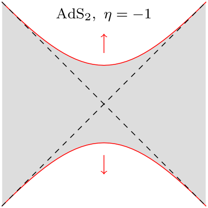
In particular, the Sachdev-Ye-Kitaev (SYK) model Sachdev and Ye (1993); Kitaev (2015c, a, b) in the double-scaling limit Cotler et al. (2017); Erdős and Schröder (2014), called the DSSYK model Berkooz et al. (2019, 2018), is a remarkable testing ground to develop concepts and techniques to study lower-dimensional quantum gravity from a concrete and solvable (through chord diagram methods Berkooz et al. (2019, 2018)) boundary theory relevant for holography beyond AdS/CFT, which might carry some relevant lessons in higher dimensional holography. Key insights to understand the DSSYK model and its bulk dual include the double-scaled Lin (2022); Xu (2024b); Cao and Gao (2025) and chord Lin and Stanford (2023) von Neumann algebras; the quantum group structure Almheiri and Popov (2024); Schouten and Isachenkov (2025); Belaey et al. (2025b); Berkooz et al. (2023); Blommaert et al. (2024); van der Heijden et al. (2025); Krylov complexity Rabinovici et al. (2023); Ambrosini et al. (2025, 2024); Heller et al. (2024); Aguilar-Gutierrez (2025a); Aguilar-Gutierrez and Xu (2026); Aguilar-Gutierrez (2025c); Xu (2024b); Balasubramanian et al. (2024); Forste et al. (2025); Aguilar-Gutierrez (2026); Bhattacharjee et al. (2023); Nandy (2024); Anegawa and Watanabe (2024); Aguilar-Gutierrez (2024c); Heller et al. (2025); Fu et al. (2025); Aguilar-Gutierrez et al. (2026); Xu (2024a) for operators Parker et al. (2019) and states Balasubramanian et al. (2022) (see recent reviews in Nandy et al. (2025); Baiguera et al. (2025); Rabinovici et al. (2025)); algebraic entanglement entropy Tang (2024); Aguilar-Gutierrez (2025b). However, there has been active debate about the specific bulk dual to the DSSYK model. The most-discussed bulk dual proposals include sine dilaton gravity Blommaert et al. (2025c, 2024, a, b); Blommaert and Levine (2025); Bossi et al. (2024); Blommaert et al. (2025d); Cui and Rozali (2025); Arundine (2025), and de Sitter (dS) space through different approaches, including Schwarzschild-dS₃ space Narovlansky and Verlinde (2023); Verlinde (2025); Verlinde and Zhang (2024); Narovlansky (2025); Blommaert et al. (2025d); Tietto and Verlinde (2025); Aguilar-Gutierrez (2024c), and dS₂ space as a s-wave reduction of dS₃ space, where the DSSYK model is conjectured to live in the stretched cosmological horizon (illustrated in Fig. 1 (d)) which is defined as a timelike codimension-one surface with Dirichlet boundary conditions somewhere in the static patch very close to the cosmological horizon, possibly a few Planck’s lengths away Susskind (2021, 2022, 2023c); Lin and Susskind (2022); Rahman (2022); Rahman and Susskind (2023, 2024b, 2024a); Sekino and Susskind (2025); Miyashita et al. (2025); Tietto and Verlinde (2025); Herderschee and Kudler-Flam (2025). Other interesting approaches can be found in e.g. Milekhin and Xu (2024, 2025); Narovlansky (2025); Okuyama (2025); Yuan et al. (2025); Aguilar-Gutierrez (2025b); Gubankova et al. (2025); Ahn et al. (2025).

At a first glance, it might seem the diversity of bulk dual proposals for the same boundary theory means that at least some of them might be incorrect. However, they are not necessarily incompatible with one another Aguilar-Gutierrez (2025c); Blommaert et al. (2025d); Aguilar-Gutierrez (2024b, 2025b). For instance, concrete connections between dS₃ space holography with sine dilaton gravity as its world-sheet theory and complex Liouville string Collier et al. (2025a, c, b, d, e, f) and the SYK model as a collective field theory was recently investigated in Blommaert et al. (2025d). To fully understand the DSSYK model, the relationship between these different proposals needs to be closely studied.

Addressing Susskind’s Conjectures

A prominent member in this family of proposals, initiated by the work of Susskind Susskind (2021), seemingly has very different features from the others Rahman and Susskind (2023). Whether it fits with sine dilaton gravity and other dS₃ proposals, or if it is incompatible with the other proposals is not well-understood. According to Susskind (2021), there are specific properties expected in dS holography that are realized by the DSSYK model at infinite (Boltzmann) temperature. Namely, Susskind (2021) postulates the following conjectures:

1. There is a RT formula in dS space that takes the same form as in AdS space when the asymptotic boundary is replaced by the stretched horizon.

2. The scrambling time in the boundary theory dual to dS space, as measured by the operator size of fundamental operators in the theory Roberts et al. (2018), which is linearly related to the out-of-time-ordered correlators (OTOCs) of the same operators Roberts et al. (2018), is of the order of the dS length scale.

3. There is a similar (hyper)fast growth of (some notion of) complexity associated to the exponential growth of the dS scale factor.

4. The SYK model at infinite (Boltzmann) temperature and with a scaling $p\sim N^{\alpha}$, where $p$ is the number of all-to-all interactions, $N$ the total number of fermions, and $0<\alpha<1$, satisfies the above properties.

The motivation for the hyperfast properties and the infinite temperature limit comes from the fact that a surface at a finite radial distance in a gravitational spacetime experiences a Tolman temperature Tolman (1928, 1933); Tolley (2020); Tolman and Ehrenfest (1930) with a redshift factor which diverges when the surface is close to the horizon. The temperature scale controls the rate of growth or decay of correlation functions, which would therefore lead to the hyperfast scrambling of OTOCs. This suggests that a boundary theory dual located at the cosmological stretched horizon should not be of the $k$-local type defined in Susskind (2021), where $k$ is an order one parameter in the $N\gg 1$ limit, and it represents the power of fundamental operators appearing in the Hamiltonian of the system. Indeed, if $k$ is fixed in the large $N$ limit, the scrambling time scales with $\log N$ Maldacena et al. (2016), and circuit complexity grows linearly in time Susskind (2016), while the CV proposal in dS space Jørstad et al. (2022) suggests it should grow faster than linear and it should end at a given static patch time with respect to the stretched horizon Susskind (2021). In the SYK proposal of Susskind (2021), we need to allow $p$ (which is the analog of $k$) to scale with $N$. In particular, when $p=N^{\alpha=1/2}$ the above conjecture suggests that the DSSYK model may be a specific example of boundary theory in stretched horizon holography Susskind (2021).

The stretched horizon conjectures are seemingly in tension with the DSSYK model being located at the asymptotic boundaries of an effective AdS₂ black hole in sine dilaton gravity Blommaert et al. (2025c) (as well as some entropic considerations Rahman and Susskind (2023)). Nevertheless, there is a specific regime in sine dilaton gravity where the theory reduces Jackiw-Teitelboim (JT) Jackiw (1985); Teitelboim (1983) gravity and to dS JT gravity Blommaert et al. (2025a); Heller et al. (2025). This limit in the bulk corresponds to zooming in the UV regime in the energy spectrum of the DSSYK model. However, the boundary theory would be located at $\mathcal{I}^{\pm}$ when taking the appropriate limit Blommaert et al. (2025a); Heller et al. (2025). In contrast, the boundary theory would be located at the stretched horizon in Susskind’s proposal. The tension between them is closely related to dS₂/CFT₁ and static patch holography in dS₂ space.

To move the asymptotic boundary from $\mathcal{I}^{\pm}$ to inside the static patch, we cannot restrict ourselves to $T^{2}$ deformations, since they lead to a complex energy spectrum once the theory reaches a Killing horizon McGough et al. (2018). However, it was recently realized by Ali Ahmad et al. (2025) that by applying a two-step process the boundaries can pass behind the horizon of asymptotically AdS₃ black holes through a combination of $\text{T}\overline{\text{T}}$ and $\text{T}\overline{\text{T}}+\Lambda_{2}$ deformations (which have been recently updated to $T^{2}+\Lambda_{3}$ deformations Silverstein and Torroba (2024)). In this process, the corresponding boundaries move from the asymptotic region to the black hole horizon through a $\text{T}\overline{\text{T}}$ deformation, and then from the horizon towards the singularity through a $\text{T}\overline{\text{T}}+\Lambda_{2}$ deformation. This procedure was recently applied in dS₃ holography by Chang et al. (2025); albeit without a concrete boundary theory in dS₃/CFT₂.

Thus, a natural way to resolve this tension is based on finite cutoff holography, by $T^{2}$ deforming the DSSYK model in the UV limit of its energy spectrum and implementing a lower dimensional version of $\text{T}\overline{\text{T}}+\Lambda_{2}$ deformations Gorbenko et al. (2019); Shyam (2022); Coleman et al. (2022); Silverstein (2022); Batra et al. (2024) to place the boundary theory near the cosmological horizon of dS₂ space.

Results in This Work

In summary, we study chord Hamiltonian deformations in the DSSYK model. We focus on the boundary description with guidance from finite cutoff holography for general dilaton gravity theories; and including the infrared (IR) and UV triple-scaling limits in the DSSYK model, which are associated to JT and dS JT gravity respectively. This allows us to investigate the thermodynamic properties and dynamical observables, particularly correlation functions, in the deformed chord theory associated to a finite cutoff in the bulk dual of the DSSYK model, while allowing general counterterms in the bulk to study their role in the holographic dictionary. We deduce the Krylov basis in the deformed theory, Krylov complexity and the corresponding representation of the chord operators under a Hamiltonian deformation, as well as the entanglement entropy between the double-scaled algebras in the deformed theory. At last, these steps allow us to realize Susskind’s stretched horizon proposal from the UV triple-scaling limit Aguilar-Gutierrez (2025b).

To elaborate on the summary, we first present a more complete derivation of the flow equation for the energy spectrum of the deformed boundary theory following up our companion work Aguilar-Gutierrez (2024b) based on finite cutoff holography for dilaton gravity theories in Gross et al. (2020b, a); Iliesiu et al. (2020). For that, we consider the Hamilton-Jacobi (HJ) equation in a generic dilaton-gravity theory and we derive the flow equation encoding the energy spectrum of the dual. In contrast to the previous literature Gross et al. (2020b, a); Iliesiu et al. (2020); Griguolo et al. (2022, 2025), we allow the counterterm in the bulk action to be modified when the boundary radial cutoff is finite. This results in more general Hamiltonian deformations in the boundary dual, including as special cases one-dimensional $T^{2}$ deformations and a lower dimensional analog of $\text{T}\overline{\text{T}}+\Lambda_{2}$, which we refer to as $T^{2}+\Lambda_{1}$ deformations. This construction extends the holographic dictionary between the DSSYK model and a generic dilaton-gravity theory dual at finite cutoff. We analyze the thermodynamic properties of the deformed model from its partition function (including the density of states, microcanonical temperature, and heat capacity). A summary of the thermodynamics of the deformed model is shown in Fig. 2. Since the chord Hamiltonian is deformed, the chord number basis used to tridiagonalize the seed Hamiltonian does not do the same in the deformed theory. We will also derive the chord basis that is associated to the length of an Einstein-Rosen bridge in the dual AdS₂ black hole (which we refer to as a “wormhole length”) at a finite cutoff, which is the Krylov basis Balasubramanian et al. (2022), and we study the representation of operators in the chord algebra. We use these results to evaluate Krylov spread complexity Balasubramanian et al. (2022) in the HH state of the deformed theory, which reproduces the wormhole length in the bulk at finite cutoff. We proceed evaluating $n$-point correlation functions. We find that in the semiclassical limit, they have the same functional dependence as the seed theory, but the parameters involving the “fake” temperature Blommaert et al. (2025c) (also called “tomperature” Susskind (2021), which is associated to the decay rate of correlation functions) contain a redshift factor, associated to the Tolman temperature at a finite distance in the bulk McGough et al. (2018); Anninos and Harris (2022). Lastly, we evaluate the von Neumann entropy with respect to a density matrix associated to the chord number of the DSSYK model. The algebraic entanglement entropy is holographic, it matches the dilaton in JT gravity and dS JT gravity at a finite cutoff when we restrict to the IR and UV triple-scaling limits in the chord theory.

In particular, when applying our results in the UV limit of the DSSYK model, we realize Susskind’s proposal for stretched horizon holography Susskind (2021), by implementing the $T^{2}$ and $T^{2}+\Lambda_{1}$ deformations, and taking a limit in deformation parameter such that the boundary is placed inside the static and close to the cosmological horizon. The thermodynamic properties of the model match those in dS₂ JT gravity at a finite cutoff. Due to the fake temperature being infinite, the rate of growth of OTOCs and Krylov spread complexity are enhanced; the scrambling time is order one in units of the dS length scale, instead of order $\log N$ expected for a fast scrambler Susskind (2021) (which would diverge in the DSSYK model). The Krylov spread complexity also reproduces the minimal length between the finite Dirichlet boundaries in dS₂, and in the case of the $T^{2}+\Lambda_{1}$ deformed theory, it reaches a maximum value at a time of order of the dS length scale expected for hyperfast complexity growth Jørstad et al. (2022). Meanwhile, the algebraic entanglement entropy for the chord number state agrees with the RT formula for dS₂ JT gravity if the boundaries are in the Milne patch of dS₂ (Fig. 1 (c)). The cosmological horizon limit reproduces the Gibbons-Hawking (GH) entropy of dS₃ space. However, if the boundaries are located in the static patch the RT formula in dS₂ does not apply, the dilaton at the minimal extremal surface becomes trivial (see Sec. 6.4). However, in higher dimensions there are more possible entangling surfaces where Susskind’s conjecture might apply. Our study takes the dS₂ geometric perspective instead of a dS₃ embedding, whose precise connection with the DSSYK model is actively debated Blommaert et al. (2025d); Rahman and Susskind (2023); Narovlansky and Verlinde (2023).

A summary comparing our results and the conjectures in Susskind (2021) is displayed in Tab. 1.

Conjecture	Confirmation in	Details
	Deformed DSSYK
Hyperfast complexity		Sec. 6.2
growth (iii+iv)
Hyperfast scrambling		Sec. 6.3
(ii+iv)
Validity of RT formula using	$\times$	Sec. 6.4
the stretched horizon (i+iv)

Table 1: Comparison between the (i-iv) conjectures in Susskind (2021), which were explained above, and the explicit realization of the cosmological stretched horizon from the $T^{2}+\Lambda_{1}$ deformation of the UV limit of the DSSYK model, corresponding to the assumption (iv). Two out of the three remaining conjectures are satisfied in this model. Further details can be found in the respective sections.

In addition, we study other generalizations and additional technical details in the appendices. In particular, we study the consequences of interpreting the results in terms of sine dilaton gravity in finite cutoff holography. The energy spectrum generically becomes complex-valued since the bulk metric and dilaton at the cutoff location are complex-valued. In those cases, there is no Lorentzian evolution, rather than the deformed theory being non-unitary, so the DSSYK Hamiltonian is not isometrically dual to a canonically quantized Arnowitt–Deser–Misner Arnowitt and Deser (1959); Arnowitt et al. (1960c, d, b, a, 1961a, 1961b) (ADM) Hamiltonian in the bulk, which is the generator of time translations. We adopt a similar prescription as in Cauchy slice holography Araujo-Regado et al. (2023); Araujo-Regado (2022); Soni and Wall (2024); Araujo-Regado et al. (2025), where the stress tensor is allowed to be complex-valued. In contrast to previous literature, the $T^{2}$ deformation parameter is generically a complex number, and it can take both positive and negative values (without an auxiliary geometric extension Apolo et al. (2023, 2024)). Later, we $T^{2}$ deform the Almheiri-Goel-Hu (AGH) model Almheiri et al. (2024), which is a simplification of the DSSYK model in the $q\rightarrow 1$ described by the Heisenberg-Weyl algebra. This integrable analog of the DSSYK model allows for analytic evaluations of correlation functions beyond the semiclassical limit.

Outline

The paper is organized as follows. In Sec. 2, we introduce Hamiltonian deformations in holographic quantum mechanics based on moving the HJ equation of the dual dilaton graviton theory with Dirichlet boundary conditions, and we study its thermodynamic properties. In Sec. 3, we specialize the results in the DSSYK model to deduce a chord basis associated with a bulk geodesic in finite cutoff holography, and the representation of the chord operators after the deformation. We also evaluate the Krylov spread complexity of the HH state. In Sec. 4 we evaluate correlation functions, including its semiclassical and its triple-scaling limits. In Sec. 5, we investigate the entanglement entropy between the double-scaled algebras in the deformed DSSYK model, and their holographic interpretation. In Sec. 6 we apply our previous results to realize the stretched horizon proposal of Susskind. We then conclude in Sec. 7 with a summary of our findings, and some relevant future directions.

In addition, App. A contains a summary of the notation used in the manuscript. In App. B we provide more details about the derivation of spacelike and timelike extremal geodesic lengths connecting the asymptotic boundaries of an effective AdS₂ black hole. App. C discusses reality conditions in sine dilaton gravity at a finite cutoff. In App. D we investigate an additional chord number basis, different from the Krylov basis, which has an interpretation in finite cutoff holography. In App. E we explore chord Hamiltonian deformations in the presence of ETW branes and Euclidean wormholes in the bulk. In App. F we $T^{2}$-deform the AGH model to study its thermodynamics and correlation functions. At last, in App. G we discuss the first law of thermodynamics in the deformed DSSYK.

2 Dilaton Gravity at Finite Cutoff and its Boundary Dual

Before specializing in the DSSYK model, we generalize previous studies of $T^{2}$ deformations for holographic (0+1)-dimensional models Gross et al. (2020b, a); Zhang and Cai (2023) assuming a dual dilaton gravity model with Dirichlet boundary conditions. In this section, we are particularly interested in deriving the energy flow equation in holographic quantum mechanics with a Hamiltonian deformation, and to study its semiclassical thermodynamics. In particular, one recovers a lower-dimensional analog of $\text{T}\overline{\text{T}}$ and $\text{T}\overline{\text{T}}+\Lambda_{2}$ deformations as special cases.

Outline

In Sec. 2.1, we study HJ equation in dilaton gravity theories and the associated flow equation. In Sec. 2.2 we study its solutions, including one-dimensional $T^{2}$ deformations and we propose a “$T^{2}+\Lambda_{1}$” deformation in the DSSYK model, which can be interpreted as pushing the finite cutoff inside the black hole horizon/ outside the cosmological horizon. In Sec. 2.3 we study the thermodynamic properties of the deformed theories, specializing to the DSSYK model for concreteness. In addition, the reader is referred to App. C for details on the reality conditions to implement the chord Hamiltonian deformations from sine dilaton gravity at a finite cutoff.

2.1 Hamiltonian Deformations from Finite Cutoff Holography

Our first goal is to derive the flow equation controlling the evolution of the energy spectrum of a (0+1)-dimensional system dual to a generic dilaton gravity theory of the form

$$I_{\rm E}\equiv -\frac{\Phi_{0}}{16\pi G_{N}}\quantity(\int_{\mathcal{M}}\mathrm{d}^{2}x\sqrt{g}\mathcal{R}+2\int_{\partial\mathcal{M}}\mathrm{d}x\sqrt{{h}}K)$$ (1)

$$-\frac{1}{16\pi G_{N}}\quantity(\int_{\mathcal{M}}\mathrm{d}^{2}x\sqrt{g}\quantity(\Phi\mathcal{R}+U(\Phi))+2\int_{\partial\mathcal{M}}\mathrm{d}x\sqrt{h}\quantity(\Phi_{B}K-\sqrt{G(\Phi_{B})}))\penalty 10000\ ,$$

where the first line is a topological term, $U(\Phi)$ and $G(\Phi_{B})$ are generic $C^{\infty}$ functions; $G_{N}$ in being the two-dimensional Newton’s constant; $\mathcal{M}$ is the spacetime manifold, $\partial\mathcal{M}$ is the location of the radial cutoff boundary where we impose Dirichlet boundary conditions on the dilaton and the induced metric,

$$\partial\mathcal{M}:\quad\Phi=\Phi_{B}\penalty 10000\ ,\quad h_{\mu\nu}\quad\text{fixed}\penalty 10000\ .$$ (2)

This allows us to generalize the flow equation in Gross et al. (2020b) for dilaton-gravity theories without AdS boundary conditions, which is motivated by the proposed duality between sine dilaton gravity and the DSSYK model Blommaert et al. (2024). One should note that a canonical choice of the counterterm is

$$G(\Phi_{B})^{\rm(others)}=\int^{\Phi_{B}}\mathrm{d}\Phi\penalty 10000\ U(\Phi)\penalty 10000\ ,$$ (3)

which guarantees the on-shell action is finite when $\Phi_{B}\gg 1$; however, we will not make this restriction in deriving the flow equation below, since we investigate cases where $\Phi_{B}$ is a finite cutoff, instead of a radial regulator of the asymptotic boundary. Also, note that in the following one may allow $g_{\mu\nu}$ and $\Phi\in\mathbb{C}$; which is the case of interest for sine dilaton gravity at finite cutoff. We will discuss this case in detail in App. C.

The strategy proposed in Hartman et al. (2019) is to recover the $T^{2}$ flow equation from the HJ equation controlling radial evolution along the flow. For this reason, we will consider the dilaton-gravity theory as the input for defining the deformed DSSYK model. Note that while we implement a similar strategy as Hartman et al. (2019); Gross et al. (2020b) to define the Hamiltonian deformations in the boundary theory, the crucial difference with previous approaches in the derivation of the flow equation from finite cutoff holography is that we do not require AdS asymptotics in the bulk, which is the reason for allowing the general counterterm $G(\Phi)$ in (1), leading to a larger class of deformations than the $T^{2}$ case.

We begin considering the general variation of an action of the form (1), given by

$$\delta I_{\rm E}= -\frac{1}{16\pi G_{N}}\int_{\mathcal{M}}\mathrm{d}^{2}x\sqrt{g}\quantity[\mathcal{E}^{\mu\nu}\delta g_{\mu\nu}+\mathcal{E}_{\Phi}\delta\Phi]+\int_{\partial\mathcal{M}}\mathrm{d}\tau\sqrt{h}\quantity[\frac{1}{2}\tilde{T}^{ab}\delta h_{ab}+\mathcal{O}_{\Phi_{B}}\delta{\Phi_{B}}]\penalty 10000\ ,$$ (5)

where

$$\mathcal{E}_{\mu\nu} \equiv\nabla_{\mu}\nabla_{\nu}\Phi-g_{\mu\nu}\nabla^{2}\Phi+\frac{1}{2}g_{\mu\nu}U(\Phi)\penalty 10000\ ,$$ (6)

$$\mathcal{E}_{\Phi} \equiv\mathcal{R}+\partial_{\Phi}U(\Phi)\penalty 10000\ .$$ (7)

Here we have introduced the Brown-York (BY) Brown and York (1993) stress tensor and the scalar operator conjugate to $\Phi$, which we denote respectively as:

$$\tilde{T}^{ab} \equiv\frac{2}{\sqrt{h}}\frac{\delta I_{E}}{\delta h_{ab}}=\frac{2}{\sqrt{h}}\quantity(\pi^{ab}+\frac{\sqrt{h}}{16\pi G_{N}}\sqrt{G(\Phi_{B})}h^{ab})\penalty 10000\ ,$$ (8a)

$$\mathcal{O}_{\Phi_{B}} \equiv\frac{1}{\sqrt{h}}\frac{\delta I_{E}}{\delta{\Phi_{B}}}=\frac{1}{\sqrt{h}}\quantity(\pi_{\Phi_{B}}+\frac{\sqrt{h}\penalty 10000\ G^{\prime}({\Phi_{B}})}{16\pi G_{N}\sqrt{G({\Phi_{B}})}})\penalty 10000\ ,$$ (8b)

where $G^{\prime}({\Phi_{B}})\equiv\derivative{G({\Phi_{B}})}{\Phi_{B}}$; and $\pi_{\Phi_{B}}$ and $\pi_{ab}$ are the canonical momenta of $h_{ab}$ and ${\Phi_{B}}$, defined as

$$\pi^{ab} \equiv-\frac{\sqrt{h}}{16\pi G_{N}}h^{ab}n^{c}\nabla_{c}{\Phi_{B}}\penalty 10000\ ,\quad\pi_{\Phi_{B}}\equiv-\frac{\sqrt{h}}{8\pi G_{N}}K\penalty 10000\ .$$ (9)

We can now study the HJ equation controlling the radial equation of the on-shell solutions. Using the general variation (5) evaluated on-shell (i.e. $\mathcal{E}_{\mu\nu}=0$, $\mathcal{E}_{\Phi}=0$), in the strict large $N\gg 1$ limit in the boundary theory, $G_{N}\rightarrow 0$ in the bulk, we recover

$$\partial_{\Phi_{B}}I_{\rm E}^{\rm(on)}=\int_{\partial\mathcal{M}}\mathrm{d}\tau\sqrt{h}\quantity[\frac{1}{2}\tilde{T}^{ab}\partial_{\Phi_{B}}h_{ab}+\mathcal{O}_{\Phi_{B}}]\penalty 10000\ ,$$ (10)

and we have to implement the ADM Hamiltonian constraint $\mathcal{H}$ for general dilaton gravity theories (1), which we evaluate at the cutoff location, and it is given by Grumiller and McNees (2007)

$$\mathcal{H} \equiv 6\pi G_{N}\pi_{\Phi_{B}}\pi^{\tau\tau}-\frac{U(\Phi_{B})}{16\pi G_{N}}=0\penalty 10000\ .$$ (11)

This constraint leads to the following relation for the dilaton source in (8b):

$$\mathcal{O}_{\Phi_{B}}=\frac{U(\Phi_{B})+\quantity(\frac{8\pi G_{N}}{G(\Phi_{B})}\tilde{T}^{\tau}_{\tau}-1)G^{\prime}({\Phi_{B}})}{16\pi G_{N}\sqrt{G({\Phi_{B}})}\quantity(\frac{8\pi G_{N}}{G({\Phi_{B}})^{2}}\tilde{T}^{\tau}_{\tau}-1)}\penalty 10000\ .$$ (12)

Following the procedure of Gross et al. (2020a), we need to identify the scaling of the different terms in (10) with respect to $r_{B}$. Similar to Hartman et al. (2019); Gross et al. (2020b), we recognize that at the finite boundary, $\Phi_{B}$, we should have the following scaling for the metric and the stress tensor given the counterterm (1),

$$\sqrt{h}=\sqrt{G(\Phi_{B})}\sqrt{\gamma}\penalty 10000\ ,\quad\tilde{T}_{\tau\tau}=\sqrt{G(\Phi_{B})}\penalty 10000\ T_{\tau\tau}\penalty 10000\ ,$$ (13)

which is a choice of normalization to match the boundary metric in the bulk to the metric of the boundary theory. (13) corresponds to a natural general generalization of the AdS₂ boundary conditions (with the corresponding $G(\Phi_{B})=\Phi_{B}^{2}$). Our proposal for extending the holographic dictionary at finite cutoff beyond AdS (13) agrees with Griguolo et al. (2025) using a different method that results in the same flow equation from general dilaton gravity theories at finite cutoff, which appeared after our results in Aguilar-Gutierrez (2024b).

Next, we use that in 1D we can express the following relation Gross et al. (2020b),

$$I_{E}=\int\mathrm{d}\tau\penalty 10000\ \sqrt{\gamma}T_{\tau}^{\tau}=\int\mathrm{d}\tau\penalty 10000\ \sqrt{\gamma}E_{y}\penalty 10000\ ,$$ (14)

where $\gamma_{ij}$ is the background metric of the 1D quantum mechanical theory, and $T_{ij}$ the corresponding boundary stress tensor, and in the last equality we use the fact that in (0+1)-dimensions, $T^{\tau}_{\tau}\equiv E_{y}$ which denotes the energy spectrum of the deformed theory, $y$ denotes a deformation parameter, which we define below. This allows us to express the HJ equation (11) as

$$\partial_{\Phi_{B}}\int_{\partial\mathcal{M}}\mathrm{d}\tau\sqrt{\gamma}\penalty 10000\ T^{\tau}_{\tau}=\int_{\partial\mathcal{M}}\mathrm{d}\tau\sqrt{\gamma}\frac{G^{\prime}(\Phi_{B})\quantity(\quantity(\frac{8\pi G_{N}}{G(\Phi_{B})}T^{\tau}_{\tau})^{2}-1)+U(\Phi_{B})}{2\quantity(\frac{8\pi G_{N}}{G(\Phi_{B})}\penalty 10000\ T^{\tau}_{\tau}-1)}\penalty 10000\ .$$ (15)

Using the relation (14), we identify that (15) can then be expressed as a flow equation for the spectrum of the boundary theory

$$\boxed{\partial_{y}E_{y}=\frac{(E_{y})^{2}+(\eta-1)/y^{2}}{2(1-yE_{y})}\penalty 10000\ ,}$$ (16)

where we have defined the parameters

$$y\equiv 8\pi G_{N}/G(\Phi_{B})\penalty 10000\ ,\quad\eta\equiv U(\Phi_{B})/G^{\prime}(\Phi_{B})\penalty 10000\ .$$ (17)

Note that while $E_{y}$ depends on both $y$ and $\eta$, where the latter is not completely determined by $y$. The functional dependence on the parameter $\eta$ will be implicit in all expressions involving $y$ to lighten the notation.

The above relation can be interpreted as a flow equation (16) for the energy spectrum of the boundary dual to the dilaton gravity theory at finite cutoff. Indeed, (16) takes the same form as other places in the literature (see e.g. Gross et al. (2020a); Iliesiu et al. (2020)) which are restricted to $\eta=U(\Phi_{B})/G^{\prime}(\Phi_{B})=1$. The latter choice of counterterm $G^{\prime}(\Phi_{B})=U(\Phi_{B})$ leads to a finite on-shell action in general dilaton-gravity theories with asymptotic Dirichlet boundaries Grumiller and McNees (2007). Meanwhile, the case $\eta=-1$ can be used when the cutoff surface is located at some finite $r_{B}$, so there is no issue with the renormalization of the on-shell action, while keeping the same holographic identification for the deformation parameter (17). We remark that the deformation parameter (17) and the flow equation (16) generalize the results in Gross et al. (2020a) which are a special case of this formulation, corresponding to a class of asymptotically AdS dilaton gravity theories.

Deformed Boundary Hamiltonian

We promote (16) to an operator relation in the quantum theory as

$$\partial_{y}\hat{H}_{y}=\hat{\Theta}(\hat{H}_{y},y)\penalty 10000\ ,\quad\hat{\Theta}=\frac{1}{2}\quantity(\hat{H}_{y}^{2}+y^{-2}(\eta-1))\quantity(1-y\hat{H}_{y})^{-1}$$ (18)

where $\hat{\Theta}(\hat{H}_{y},y)$ is the $\text{T}\overline{\text{T}}$ deformation operator Kruthoff and Parrikar (2020), and $\hat{H}_{y}$ is the Hamiltonian deformation of the boundary theory.

2.2 Solutions to the Flow Equation

First, notice from (17) that $\eta=\eta(y)$ generically. As mentioned in the introductions, when we deformed the boundary theory starting at the asymptotic boundary in the bulk, we need to set $G(\Phi_{B})$ as in (3). However, once we reach a finite cutoff value $\Phi_{B}$, we can allow $G(\Phi_{B})$ to be more arbitrary, which defines a set of possible deformed theories. Below we specialize in one of them due to its applications for studying the stretched horizon conjecture of Susskind Susskind (2021).

We will be interested in the case $\eta=\pm 1$, as this allows us to introduce an analogous type of deformation as $\text{T}\overline{\text{T}}(+\Lambda_{2})$ Silverstein and Torroba (2024); Batra et al. (2024); Gorbenko et al. (2019); Coleman et al. (2022) deformations, which we define below as

$$T^{2}(+\Lambda_{1})\penalty 10000\ {\rm deformations}:\quad U(\Phi)\quad\text{fixed}\penalty 10000\ ,\quad G(\Phi_{B})\rightarrow\pm G(\Phi_{B})\penalty 10000\ ,$$ (19)

resulting in $\eta=\pm 1$ in (16). We note that the solutions to the flow equation when $\eta$ is a fixed parameter are

$$E_{y}=\frac{1}{y}\quantity(1\pm\sqrt{\eta-2yf(E)})\penalty 10000\ .$$ (20)

where $f(E)$ is a function determined by initial conditions.

$T^{2}$ deformation

The best studied case from the lower dimensional perspective corresponds to $\eta=+1$. The deformed energy spectrum in terms of the seed theory takes the form

$$E^{\eta=+1}_{y}(\theta)=\frac{1}{y}\quantity(1\pm\sqrt{1-2yE})\penalty 10000\ .$$ (21)

The solution with a relative $-$ sign represents the energy spectrum at a finite cutoff in the holographic dual (see e.g. McGough et al. (2018); Hartman et al. (2019)), as seen from the on-shell action (32), which is smoothly connected to the seed theory in the limit $y\rightarrow 0$. Meanwhile, the solution with the relative $+$ sign represents the complementary spacetime region with respect to the finite cutoff. Both are represented in Fig. 1.

$\text{T}\overline{\text{T}}+\Lambda_{1}$ deformations

When $\eta=-1$, this corresponds to a s-wave reduction of $\text{T}\overline{\text{T}}+\Lambda_{2}$ deformations Gorbenko et al. (2019); Coleman and Shyam (2021); Silverstein (2022); Batra et al. (2024); Ali Ahmad et al. (2025), which we refer to as $T^{2}+\Lambda_{1}$ deformations. In this case $\eta=-1$ means that at some point along the flow, we modify the boundary counterterm in the action (1) with $G(\Phi_{B})\rightarrow-G(\Phi_{B})$, while retaining the same dilaton potential $U(\Phi)\rightarrow U(\Phi)$.

In particular, we consider a transition between the perturbative branch (21) in the $\eta=+1$ case to the $\eta=-1$ case when the square-root term in (21) vanishes, corresponding to

$$y=y_{0}\equiv 1/(2E)\penalty 10000\ .$$ (22)

By demanding continuity in (20), the energy spectrum then takes the form

$$E^{\eta=-1}_{y}=\frac{1}{y}\quantity(1\pm\sqrt{2yE-1})\penalty 10000\ .$$ (23)

As before, there are two relative signs; both of them are continuously connected to the $T^{2}$ deformation since the square root factor in either case vanishes for the transition point of the deformation parameter (22). We will specialize in the one with the relative $+$ sign for concreteness, and to probe the cosmological patch in the dS₂ space limit of the bulk. However, it is equally valid to adopt the $-$ sign; similar to the $T^{2}$ case, the different signs simply correspond to different bulk regions Ali Ahmad et al. (2025). In particular, the relative $-$ sign in the $\eta=-1$ in the (23) spectrum corresponds to the bulk region connecting the asymptotic boundary to the finite cutoff inside the horizon, while the $+$ relative sign in (23) corresponds to the complement. The relative $+$ solution in the $\eta=-1$ case is illustrated in Figs. 1b and 1d.

Note that since there are no modifications in the dilaton potential in the $\eta=-1$ case, it describes the same bulk metric as its $\eta=+1$ analog, similar to Ali Ahmad et al. (2025); Chang et al. (2025) (in contrast to other approaches Coleman et al. (2022); Batra et al. (2024); Gorbenko et al. (2019); Shyam (2022); Silverstein and Torroba (2024) which can be realized by changing the dilaton potential). In fact, the BY stress tensor evaluated at the radial boundary $\Phi_{B}$ ($\tilde{T}_{\tau}^{\tau}=G(\Phi_{B})T^{\tau}_{\tau}$ (13)) changes sign during the transition between $\eta=+1$ and $\eta=-1$. This means that the normal vector to the constant $r_{B}$ surface changes from spacelike to timelike as explained in Ali Ahmad et al. (2025). Thus, the finite cutoff crosses the horizon once we turn on the $T^{2}+\Lambda_{1}$ deformation. We illustrate the two-step bulk interpretation of the $T^{2}$ and $T^{2}+\Lambda_{1}$ deformation in Fig. 1.

(a)

(b)

(c)

(d)

Figure 1: Bulk interpretation of the $T^{2}$ and $T^{2}+\Lambda_{1}$ flow in the boundary theory describing (a,b) an AdS₂ black hole, and (c, d) dS₂ space based on the IR/UV triple-scaling limits of the deformed DSSYK in Sec. 3. The gray regions represent the parts of the bulk that are cut out. (a) By implementing the $T^{2}$ deformation, with spectrum (21), there is a finite boundary cutoff (red solid curve) in the Rindler-AdS₂ patch til it reaches the horizon. (b) We implement the $T^{2}+\Lambda_{1}$ deformation (23) which moves the boundary inside the black hole horizon. A similar procedure applies for dS₂ space for (c) $T^{2}$ and (d) $T^{2}+\Lambda_{1}$ deformations. In the latter, the cosmological stretched horizon Susskind (2021) is realized when the Dirichlet boundaries are very close to the dS₂ horizon.

2.3 Thermodynamics

In this subsection, we specialize the previous results to study the semiclassical thermodynamics of the deformed DSSYK model from its partition function to evaluate its energy spectrum, thermodynamic entropy, density of states, and heat capacity as a function of its temperature. This leads to conditions when the deformed theory is thermodynamically stable. We do not assume a specific dual dilaton gravity theory (1) to the DSSYK model in this section (see App. C for considerations in sine dilaton gravity).

Energy spectrum, entropy and temperature

Consider the partition function of the deformed DSSYK model which we evaluate in the semiclassical limit as

$$Z_{y}(\beta)\equiv\bra{\Omega}\mathrm{e}^{-\beta\hat{H}_{y}}\ket{\Omega}\underset{\lambda\rightarrow 0}{=}\int\mathrm{d}E(\theta)\penalty 10000\ \mathrm{e}^{-\beta E_{y}(\theta)}\rho(\theta)\penalty 10000\ ,$$ (24)

where $E(\theta)$ is the energy spectrum of the seed theory; $\rho(\theta)=\mathrm{e}^{S(\theta)}$ is the semiclassical density of states, and $S(\theta)$ is the thermodynamic entropy, given by Goel et al. (2023),

$$E(\theta)\equiv-\frac{2J\penalty 10000\ \cos(\theta)}{\sqrt{\lambda(1-q)}}\penalty 10000\ ,\quad S(\theta)\equiv S_{0}+\frac{2\theta}{\lambda}\quantity(\pi-\theta)\penalty 10000\ ,\quad\theta\in[0,\pi]\penalty 10000\ ,$$ (25)

where $J$, $\lambda\equiv-\log q\geq 0$ are constant parameters of the theory, which will be specified in Sec. 3.1, and we have introduced $S_{0}$, resulting from an overall normalization of the partition function. The microcanonical inverse temperature in this theory is given by

$$\beta_{y}(\theta)\equiv\derivative{S}{E_{y}}=\beta(\theta)\derivative{E}{E_{y}}\penalty 10000\ ,\quad\beta(\theta)\equiv\frac{2\pi-4\theta}{J\sin\theta}\penalty 10000\ ,$$ (26)

where there is a redshift factor is

$$\derivative{E}{E_{y}}=\begin{cases}\sqrt{1-2yE(\theta)}\penalty 10000\ ,&\eta=+1\penalty 10000\ ,\\ \sqrt{2yE(\theta)-1}\penalty 10000\ ,&\eta=-1\penalty 10000\ .\end{cases}$$ (27)

Given that $\beta_{y}$ is the periodicity of the thermal circle, the $T^{2}$ deformation effectively shrinks it. One can similarly recast (24) in the form:

$$Z_{y}(\beta)= \int\mathrm{d}E_{y}(\theta)\penalty 10000\ \mathrm{e}^{-\beta E_{y}(\theta)}\rho_{y}(\theta)\penalty 10000\ ,$$ (28a)

$$\rho_{y}(\theta) \equiv\rho(\theta)\derivative{E(\theta)}{E_{y}(\theta)}\penalty 10000\ ,$$ (28b)

where $\rho_{y}$ can be interpreted as the density of states in the deformed theory Gross et al. (2020b). Note that since the redshift factor is $\mathcal{O}(1)$, it does not modify the thermodynamic entropy which is $\mathcal{O}(\lambda^{-1})$ in the limit where $\lambda\rightarrow 0$.

We include Fig. 2 to exemplify the resulting thermodynamic properties of the $T^{2}$ deformed DSSYK model for generic values of the deformation parameter $y$ appearing in the flow equation (16) for $\eta=+1$.

(a)

(b)

(c)

(d)

Figure 2: (a) The energy spectrum (52), (b) thermodynamic entropy (25), (c) density of states (28b), and (d) heat capacity (29) for generic values of the deformation parameter $y$ (17) (shown in the legends) and fixing $\eta=+1$. We use $\lambda=10^{-4}$ in all subfigures, except in (c) where $\lambda=0.1$ for visualization purposes.

First law of thermodynamics

The previous results can be used to express variations of the energy spectrum with respect to the parameters of the model. We include details about the relevant calculations in App. G.

Heat capacity

Next, we use the previous results to determine the thermal stability of the system, using the definition of the heat capacity

$$C_{y}(\theta)\equiv-\beta_{y}(\theta)^{2}\derivative{E_{y}(\theta)}{\beta_{y}(\theta)}\penalty 10000\ .$$ (29)

For concreteness, we consider the main cases of interest where $\eta=\pm 1$ so that $E_{y}$ is given by (52) ($\eta=+1$) and (23) ($\eta=-1$) respectively, so that (29) becomes,

$$C_{y}(\theta)=\frac{\eta(J\sin\theta\beta_{y}(\theta))^{2}}{2Jy\sin\theta(\pi-2\theta)+4Jy\cos\theta(2+(\pi-2\theta)\cot\theta)+2(2+(\pi-2\theta)\cot\theta\sqrt{\lambda(1-q)})}\penalty 10000\ .$$ (30)

The argument in the numerator is positive definitive when $y\in\mathbb{R}$, $\lambda>0$ and $\theta\in[0,\pi]$. Note that the case where $\eta=+1$ has a positive heat capacity while $\eta=-1$ a negative one assuming that $E_{y}$ can be interpreted as the conserved energy spectrum of the deformed theory.

It is important to distinguish when $C_{y}(\theta)$ physically corresponds to heat capacity when performing the $T^{2}$ and $T^{2}+\Lambda_{1}$ flow. For instance in dS₂, one performs the $T^{2}$ deformation, associated with $E_{y}^{\eta=+1}$, using the Dirichlet boundaries in the Milne patch which are spacelike Chang et al. (2025); while during the $T^{2}+\Lambda_{1}$ flow, associated to $E_{y}^{\eta=-1}$, the finite cutoff boundaries are located in the static patch of dS₂ and they are timelike, so that $E_{y}^{\eta=-1}$ can indeed be associated with a quasilocal BY energy Svesko et al. (2022). Then, (30) is indeed physically a heat capacity and the system can thus be thermodynamically unstable, as found in different parts of the literature, see e.g. Sec 6.1. As additional comparison, when $\text{T}\overline{\text{T}}$ deforming CFTs, one finds negative heat capacities at high energies for $T^{2}$-deformed CFTs and quantum mechanical systems in Barbon and Rabinovici (2020); while in this system, the energy spectrum is bounded. To make more contrast, opposite observations appear in the AdS₂ case, one performs the $T^{2}$ deformation when the boundaries are timelike, and thus the system is stable since (30) indeed corresponds to a possitive heat capacity, and $T^{2}+\Lambda_{1}$ when the boundaries are spacelike, similar to Ali Ahmad et al. (2025).

Finite cutoff Holographic Interpretation

We now provide a bulk interpretation of (26) from finite cutoff holography. Let us consider the dilaton gravity theory (1), where the metric solution to the equations of motions without matter sources is

$$\mathrm{d}s^{2}=F(\Phi)\mathrm{d}\tau+\frac{\mathrm{d}\Phi}{F(\Phi)}\penalty 10000\ ,\quad F(x)=\int_{r_{h}}^{x}\penalty 10000\ U(\Phi)\mathrm{d}\Phi\penalty 10000\ ,$$ (31)

where $r_{h}$ is the horizon radius. This can be used to evaluate the on-shell action from (1), resulting in

$$I_{\rm E}^{\rm(on)}=-\frac{1}{16\pi G_{N}}\quantity(2\pi(\Phi_{0}+r_{h})+\beta\quantity(F(\Phi_{B})-\sqrt{F(\Phi_{B})\penalty 10000\ G(\Phi_{B})}))\penalty 10000\ ,$$ (32)

where we have used the fact that $\mathcal{M}$ has a disk topology when $\Phi_{0}\gg\absolutevalue{\Phi}$ everywhere. From (32) we find:

$$\beta_{T}E_{\rm BY}=\quantity(\beta\sqrt{\frac{F(\Phi_{B})}{G(\Phi_{B})}})\quantity(\frac{{G(\Phi_{B})}}{16\pi G_{N}}\quantity(1-\sqrt{\frac{F(\Phi_{B})}{G(\Phi_{B})}}))\penalty 10000\ ,$$ (33)

where we identified the inverse the BY quasi-local energy and Tolman temperature (i.e. the respective energy and temperature that an observer in a bulk spacetime would associate with a given system at a finite distance $\Phi_{B}$ from it Brown and York (1993)) as

$$E_{\rm BY}\equiv\frac{1}{16\pi G_{N}}\quantity(\sqrt{G(\Phi_{B})}-\sqrt{F(\Phi_{B})})\penalty 10000\ ,\quad\beta_{\rm T}\equiv\beta\sqrt{F(\Phi_{B})}\penalty 10000\ .$$ (34)

Comparing (34) with the microcanonical temperature of the deformed theory in (26) due to (17), we identify the parameters:

$$E_{y}=\sqrt{G(\Phi_{B})}\penalty 10000\ E_{\rm BY}\penalty 10000\ ,\quad\beta_{y}=\frac{\beta_{\rm T}}{\sqrt{G(\Phi_{B})}}\penalty 10000\ .$$ (35)

For these relations to hold, we have that

$$\lambda=8\pi G_{N}\penalty 10000\ ,$$ (36)

which is consistent with Blommaert et al. (2025d).

Thus, we find a holographic dictionary at the level of finite cutoff thermodynamics. In contrast with previous literature, we include a more general counterterm $G(\Phi_{B})$ in the above expressions, which permits the analysis for non-trivial $\eta$ in the flow equations (16).

Moreover, it follows from (35) that the specific heat in the bulk at a fixed finite radial cutoff can be expressed as

$$C_{r_{B}}\equiv-\beta_{\rm T}^{2}\derivative{E_{\rm BY}}{\beta_{\rm T}}=-(\beta_{y})^{2}\derivative{E_{y}}{\beta_{y}}=C_{y}\penalty 10000\ .$$ (37)

This means that there is a direct relation between the heat capacity in the boundary theory at a fixed deformation parameter $y$ (as well as $\eta$) (29) with respect to the heat capacity in the bulk. Similar results were recovered in related settings by Aguilar-Gutierrez et al. (2025).

Hagedorn growth

Before closing the section, we make contrast with other results in the literature, we analyze the semiclassical partition function with $\eta=-1$ (23)

$$\int_{-\frac{2J}{\lambda}}^{\frac{2J}{\lambda}}\mathrm{d}E(\theta)\penalty 10000\ \mathrm{e}^{S(\theta)-\beta E^{\eta=-1}_{y}(\theta)}=\int_{-\frac{2J}{\lambda}}^{\frac{2J}{\lambda}}\mathrm{d}E(\theta)\penalty 10000\ \mathrm{e}^{S(\theta)-\frac{\beta}{y}\quantity(1+\sqrt{2yE(\theta)-1})}\penalty 10000\ .$$ (38)

Notably, there no divergence associated to Hagedorn growth for the $T^{2}+\Lambda_{1}$ deformed theory, in contrast to other studies Ali Ahmad et al. (2025). The reason that there is no divergence even when $\beta\rightarrow 0$ is that the integration is performed over a finite energy range and the factor $\mathrm{e}^{S(\theta)}$ is finite, thus the model remains UV finite. It was interpreted by Ali Ahmad et al. (2025), that one reaches a divergence once the boundary in the dual theory reaches a curvature singularity, which is not present in JT gravity, seen as a s-wave reduction of higher dimensional charged black hole, nor in sine dilaton gravity Blommaert et al. (2024).

3 Deforming the DSSYK Model: Chord Basis, Bulk Length & Complexity

Following up the last subsection, we specialize in chord Hamiltonian deformations of the DSSYK model. We study the Krylov basis and Krylov spread complexity for the HH state in the deformed theory and show that in the semiclassical limit, it reproduces a wormhole length in finite cutoff holography.

Outline

In Sec. 3.1 we briefly review the DSSYK model, including its Hilbert space extension with matter chords. Sec. 3.2 presents the evaluation of Krylov spread complexity for the HH state from a path integral formulation of the model. It reproduces a wormhole length in finite cutoff holography. We discuss the IR/UV triple-scaling limits of the deformed theory.

In addition, we construct a chord number basis related to finite cutoff holography in App. D, as an alternative to the Krylov basis in this section that leads to similar results.

3.1 Review of the DSSYK model

In this subsection, we briefly review the DSSYK model.

The SYK model Sachdev and Ye (1993); Kitaev (2015c, a, b); Maldacena and Stanford (2016) is a system with $N$ Majorana fermions in $(0+1)$-dimensions, and $p$-body all-to-all interactions. The theory is given by

$$\hat{H}_{\rm SYK}=\mathrm{i}^{p/2}\sum_{I}J_{I}\hat{\psi}_{I}\penalty 10000\ ,$$ (39)

where $I=i_{1},\dots,\penalty 10000\ i_{p}$ is a collective index, $1\leq i_{1}<\dots<i_{p}\leq N$; and similarly $\hat{\psi}_{I}\equiv\hat{\psi}_{i_{1}}\dots\hat{\psi}_{i_{p}}$ is a string of Majorana fermions, obeying the Clifford algebra

$$\quantity{\hat{\psi}_{i},\penalty 10000\ \hat{\psi}_{j}}=2\delta_{ij}\mathbbm{1}\penalty 10000\ ;$$ (40)

and the coupling constants $J_{I}=J_{i_{1}\dots i_{p}}$ follow a Gaussian distribution

$$J_{I}=0\penalty 10000\ ,\quad\expectationvalue{J_{I}J_{J}}=\begin{pmatrix}N\\ p\end{pmatrix}^{-1}\frac{J^{2}N}{2p^{2}}\delta_{IJ}\penalty 10000\ ,$$ (41)

with $J\in\mathbb{R}$ being a constant, and the expectation values denote annealed averaging over the couplings. We also introduce matter operators, which have the form:

$$\hat{\mathcal{O}}_{\Delta} \equiv\mathrm{i}^{\frac{p^{\prime}}{2}}\sum_{I^{\prime}}K_{I^{\prime}}\hat{\psi}_{I^{\prime}}\penalty 10000\ .$$ (42)

Here $I^{\prime}=i_{1},\dots,i_{p^{\prime}}$; and $K_{I^{\prime}}$ represents Gaussian random couplings that are independent of $J_{I}$. We also define $\Delta\equiv p^{\prime}/p$, so that we can express

$$\expectationvalue{K_{I}}=0\penalty 10000\ ,\quad\expectationvalue{K_{I}J_{I^{\prime}}}=0\penalty 10000\ ,\quad\expectationvalue{(K_{I})^{2}}=\frac{\mathcal{K}^{2}}{\Delta^{2}\lambda}\begin{pmatrix}N\\ p^{\prime}\end{pmatrix}^{-1}\penalty 10000\ ,$$ (43)

where $\mathcal{K}\in\mathbb{R}$. In the following, we will set $\mathcal{K}=1$, which can be restored back with dimensional analysis. Importantly for us, once we consider the double scaling regime, where:

$$N,\penalty 10000\ p\rightarrow\infty\penalty 10000\ ,\quad q=\mathrm{e}^{-\lambda}\equiv\mathrm{e}^{-\frac{2p^{2}}{N}}\penalty 10000\ \text{fixed}\penalty 10000\ .$$ (44)

The SYK model becomes analytically solvable even away from the low energy regime; its ensemble averaged Hamiltonian moments can be described with chord diagrams techniques Berkooz et al. (2019, 2018); Cotler et al. (2017); Erdős and Schröder (2014), whose auxiliary Hilbert space without matter is

$$\mathcal{H}_{0}={\rm span}\quantity{\ket{n}\penalty 10000\ |\penalty 10000\ \penalty 10000\ n\in\mathbb{Z}_{\geq 0}}={\rm L}^{2}(\theta\in[0,\pi],\mathrm{d}\mu(\theta))\penalty 10000\ ,$$ (45)

where $n$ denotes the number of open chords at a given time slice in the chord diagram (see e.g. Berkooz and Mamroud (2025) for a review). From now on we will denote the zero-chord number state as

$$\ket{n=0}\equiv\ket{\Omega}\penalty 10000\ .$$ (46)

The auxiliary quantum mechanical theory, described by a chord Hamiltonian $\hat{H}$, contains the thermal information about the physical system, as captured by the Hamiltonian moments

$$\expectationvalue{\tr(\hat{H}_{\rm SYK}^{k})}=\bra{\Omega}\hat{H}^{k}\ket{\Omega}\penalty 10000\ ,$$ (47)

where the trace is taken over the Hilbert space states. By an appropriate orthogonal transformation, $\quantity{\ket{n}}$ can be orthonormalized (i.e. $\bra{n}\ket{m}=\delta_{nm}$), such that the Hamiltonian takes a symmetric form (see e.g. Berkooz et al. (2019))

$$\hat{H}\ket{n} =-\frac{J}{\sqrt{\lambda}}\quantity(\sqrt{[n]_{q}}\ket{n-1}+\sqrt{[n+1]_{q}}\ket{n+1})\penalty 10000\ ,$$ (48)

where $[n]_{q}\equiv\frac{1-q^{n}}{1-q}$. We can now define the chord number operator $\hat{n}$ and its conjugate momentum, $\hat{p}$:

$$\mathrm{e}^{\pm\mathrm{i}\hat{p}}\ket{n}=\ket{n\mp 1}\penalty 10000\ ,\quad\hat{n}\ket{n}=n\ket{n}\penalty 10000\ ,$$ (49)

which obey the commutation relation:

$$\quantity[\hat{n},\penalty 10000\ \mathrm{e}^{\mathrm{i}\hat{p}}]=\mathrm{e}^{\mathrm{i}\hat{p}}\penalty 10000\ ,\quad\quantity[\hat{n},\penalty 10000\ \mathrm{e}^{-\mathrm{i}\hat{p}}]=-\mathrm{e}^{-\mathrm{i}\hat{p}}\penalty 10000\ .$$ (50)

The Hamiltonian can be then expressed as

$$\hat{H}= -\frac{J}{\sqrt{\lambda}}\quantity(\mathrm{e}^{\mathrm{i}\hat{p}}\sqrt{[\hat{n}]_{q}}+\sqrt{[\hat{n}]_{q}}\mathrm{e}^{-\mathrm{i}\hat{p}})\penalty 10000\ .$$ (51)

One can also find the energy basis $\ket{\theta}$ of $\hat{H}$, whose eigenvalues are given as Berkooz et al. (2019, 2018)

$$\hat{H}\ket{\theta}=E(\theta)\ket{\theta},\quad E(\theta)\equiv-\frac{2J\penalty 10000\ \cos(\theta)}{\sqrt{\lambda(1-q)}}\penalty 10000\ ,\quad\theta\in[0,\penalty 10000\ \pi]\penalty 10000\ .$$ (52)

Solving the eigenvalue problem in (51) one can then find that the inner product between the energy basis $\quantity{\ket{\theta}}$ and the chord number $\quantity{\ket{n}}$ is given by

$$\bra{\theta}\ket{n}={\frac{H_{n}(\cos\theta|q)}{\sqrt{(q;q)_{n}}}}\penalty 10000\ ,$$ (53)

with $(a;\penalty 10000\ q)_{n}$ the q-Pochhammer symbol:

$$(a;\penalty 10000\ q)_{n}\equiv\prod_{k=0}^{n-1}(1-aq^{k})\penalty 10000\ ,\quad(a_{0},\dots,a_{N};q)_{n}\equiv\prod_{i=1}^{N}(a_{i};\penalty 10000\ q)\penalty 10000\ ,$$ (54)

and $H_{n}(x|q)$ is the q-Hermite polynomial:

$$H_{n}(\cos\theta|q)\equiv\sum_{k=0}^{n}\begin{bmatrix}n\\ k\end{bmatrix}_{q}\mathrm{e}^{\mathrm{i}(n-2k)\theta}\penalty 10000\ ,\quad\begin{bmatrix}n\\ k\end{bmatrix}_{q}\equiv\frac{(q;\penalty 10000\ q)_{n}}{(q;\penalty 10000\ q)_{n-k}(q;\penalty 10000\ q)_{k}}\penalty 10000\ .$$ (55)

The $\ket{\theta}$ basis is normalized such that

$$\bra{\theta}\ket{\theta_{0}} =\frac{1}{\mu(\theta)}\delta(\theta-\theta_{0})\penalty 10000\ ,\quad\mathbb{1}=\int_{0}^{\pi}\mathrm{d}\theta\mu(\theta)\ket{\theta}\bra{\theta}=\sum_{n=0}^{\infty}\ket{n}\bra{n}\penalty 10000\ ,$$ (56)

$$\mu(\theta) =\frac{(q,\penalty 10000\ \mathrm{e}^{\pm 2\mathrm{i}\theta};q)_{\infty}}{2\pi}\equiv\frac{1}{2\pi}(q,\penalty 10000\ q)_{\infty}(\mathrm{e}^{2\mathrm{i}\theta},\penalty 10000\ q)_{\infty}(\mathrm{e}^{-2\mathrm{i}\theta},\penalty 10000\ q)_{\infty}\penalty 10000\ .$$ (57)

For later convenience, we introduce a simple generalization when considering that the DSSYK model with matter insertions Lin (2022), which we denote as

$$\mathcal{H}_{\rm full}\equiv\bigoplus_{m=0}^{\infty}\mathcal{H}_{m}\penalty 10000\ ,\quad\mathcal{H}_{m}\equiv{\rm span}\quantity{\ket{\tilde{\Delta},n_{0},n_{1},\cdots,n_{m}}}\penalty 10000\ ,$$ (58)

where $\tilde{\Delta}=\quantity{\Delta_{1},\dots,\Delta_{m}}$ is a set of conformal dimensions, and $\Delta_{i}$ characterizes each matter chord operator $\hat{\mathcal{O}}_{\Delta_{i}}$ which is the ensemble averaged analog of the SYK operator (42).

It is also useful to define a total chord number operator

$$\hat{N}\ket{\tilde{\Delta},n_{0},\cdots,n_{m}}=\sum_{i=0}^{m}n_{i}\ket{\tilde{\Delta},n_{0},\cdots,n_{m}}\penalty 10000\ ,$$ (59)

which will be applied in later sections to evaluate correlation functions.

Next, we consider the two-sided chord Hamiltonian with $m$ operator insertions:

$$\hat{H}_{L/R}=-\frac{J}{\sqrt{\lambda}}\quantity(\hat{a}_{L/R}+\hat{a}^{\dagger}_{L/R})\penalty 10000\ ,\quad\text{where}$$ (60a)

$$\hat{a}^{\dagger}_{L}=\hat{a}^{\dagger}_{0}\penalty 10000\ ,\quad\hat{a}_{L}=\sum_{i=0}^{m}\hat{\alpha}_{i}{[\hat{n}_{i}]_{q}}q^{\hat{n}_{i}^{<}}\penalty 10000\ ,\quad\text{with}\quad\hat{n}_{i}^{<}=\sum_{j=0}^{i-1}\quantity(\hat{n}_{j}+\Delta_{j+1})\penalty 10000\ ,$$ (60b)

$$\hat{a}^{\dagger}_{R}=\hat{a}^{\dagger}_{m}\penalty 10000\ ,\quad\hat{a}_{R}=\sum_{i=0}^{m}\hat{\alpha}_{i}{[\hat{n}_{i}]_{q}}q^{\hat{n}_{i}^{>}}\penalty 10000\ ,\quad\text{with}\quad\hat{n}_{i}^{>}=\sum_{j={i+1}}^{m}\quantity(\hat{n}_{j}+\Delta_{j})\penalty 10000\ ,$$ (60c)

where the creation and annihilation operators for the chord number sectors (60) in (58) act as,

$$\hat{a}^{\dagger}_{i}\ket{\tilde{\Delta};n_{0},\dots n_{i},\dots,n_{m}} =\ket{\tilde{\Delta};n_{0},\dots,n_{i}+1,\dots n_{m}}\penalty 10000\ ,$$ (61a)

$$\hat{\alpha}_{i}\ket{\tilde{\Delta};n_{0},\dots n_{i},\dots,n_{m}} =\ket{\tilde{\Delta};n_{0},\dots,n_{i}-1,\dots n_{m}}\penalty 10000\ .$$ (61b)

For instance, in terms of the above basis, the one-particle chord Hamiltonian, corresponding to $m=1$ in (60) becomes

$$\hat{H}_{L/R}=\frac{J}{\sqrt{\lambda(1-q)}}\quantity(\mathrm{e}^{-\mathrm{i}\hat{P}_{L/R}}+\mathrm{e}^{\mathrm{i}\hat{P}_{L/R}}\quantity(1-\mathrm{e}^{-\hat{\ell}_{L/R}})+q^{\Delta}\mathrm{e}^{\mathrm{i}\hat{P}_{R/L}}\mathrm{e}^{-\hat{\ell}_{L/R}}\quantity(1-\mathrm{e}^{-\hat{\ell}_{R/L}}))\penalty 10000\ ,$$ (62)

where we expressed

$$\hat{a}_{i}^{\dagger}=\frac{\mathrm{e}^{-\mathrm{i}\hat{P}_{i}}}{\sqrt{1-q}}\penalty 10000\ ,\quad\hat{\alpha}_{i}=\sqrt{1-q}\mathrm{e}^{\mathrm{i}\hat{P}_{i}}\penalty 10000\ ,\quad q^{\hat{n}_{i}}=\mathrm{e}^{-\hat{\ell}_{i}}\penalty 10000\ ,\quad i=L,R\penalty 10000\ .$$ (63)

At last, there is an energy basis conjugate to the one-particle chord number basis, diagonalizing the two-sided Hamiltonians (60a), i.e.

$$\hat{H}_{L/R}\ket{\Delta;\theta_{L},\theta_{R}}=E(\theta_{L/R})\ket{\Delta;\theta_{L},\theta_{R}}\penalty 10000\ ,$$ (64)

where $E(\theta)$ appears in (52).

For later convenience, when discussing the IR and UV triple-scaling limits of the DSSYK model Lin (2022); Aguilar-Gutierrez (2025b), we zoom in on the edges of the energy spectrum, i.e.

$${\rm IR}:\penalty 10000\ \theta\sim\mathcal{O}(\lambda)\penalty 10000\ ,\quad{\rm UV}:\penalty 10000\ \pi-\theta\sim\mathcal{O}(\lambda)\penalty 10000\ ,$$ (65)

and we define the zero-point energy-subtracted and rescaled chord Hamiltonians in the seed theory,

$$\hat{H}_{\rm IR/UV} \equiv\evaluated{\frac{\sqrt{\lambda(1-q)}}{2J}\quantity(\pm\hat{H}+\frac{2J}{\sqrt{\lambda(1-q)}})}_{\mathcal{O}(\lambda),{\rm IR/UV}}\penalty 10000\ ,$$ (66a)

$$E_{\rm IR/UV} \equiv\evaluated{\pm\frac{\sqrt{\lambda(1-q)}}{J}E(\theta)+1}_{\mathcal{O}(1),IR}=\frac{\theta_{\rm IR/UV}^{2}}{2}\penalty 10000\ ,$$ (66b)

where $\theta_{IR/UV}\sim\mathcal{O}(\lambda)$ in the corresponding triple-scaling limit; the relative $+$ sign corresponds to the IR, while $-$ for the UV.

We will apply the above definitions to evaluate different properties and observables of the theory under a Hamiltonian deformation in the remainder of the manuscript.

3.2 Krylov Spread Complexity

We now explore the structure of the chord Hilbert space after a generic Hamiltonian deformation

$$\hat{H}\rightarrow\hat{H}_{y}\equiv f_{y}(\hat{H})\ket{\Omega}\penalty 10000\ ,$$ (67)

for some analytic function $f_{y}$. While the deformed and seed theories have the same Hilbert space, the chord basis can take different forms, and the Hamiltonian (67) can have different representations depending on the basis that we choose. For instance, consider the chord number basis where the seed theory Hamiltonian takes the form (51). The deformed chord Hamiltonian (67) for $y\neq 0$ is in general not diagonal in the chord number basis (51). Since the Hamiltonian deformation scrambles the chord basis, we search for a meaningful ordering provided by the Krylov basis. This basis allows us to minimize a so-called “cost function” associated with a general quantum state, as we explain below based on the seminal work by Balasubramanian et al. (2022), which defines Krylov spread complexity. Moreover, recent developments indicate that the Krylov spread complexity in the seed theory DSSYK model can be interpreted in terms of minimal geodesic lengths between asymptotic boundaries in the bulk dual Rabinovici et al. (2023); Lin (2022); Heller et al. (2024). We search for the corresponding interpretation of Krylov spread complexity in the finite cutoff holographic dictionary.

Cost Function

In general, following Balasubramanian et al. (2022) and Erdmenger et al. (2023) we refer to the cost function of an ordered basis $\quantity{\ket{B_{0}},\ket{B_{1}},\dots,\ket{B_{n}},\dots}$ with respect to a reference state $\ket{\psi(\tau)}$ as

$$\mathcal{C}\equiv\sum_{n=0}^{\infty}c_{n}\frac{\absolutevalue{\bra{B_{n}}\ket{\psi(\tau)}}^{2}}{\bra{\psi(\tau)}\ket{\psi(\tau)}}\penalty 10000\ ,$$ (69)

where $\quantity{c_{n}\in\mathbb{R}}$ is a monotonically increasing sequence, and we allow that the reference state evolves in complex-valued time $\tau$ as Erdmenger et al. (2023)

$$\ket{\psi(\tau)}\equiv\mathrm{e}^{-\tau\hat{\mathcal{L}}}\ket{\psi(0)}\penalty 10000\ ,$$ (70)

where $\tau\equiv\frac{\beta}{2}+\mathrm{i}t$, with $\beta$ and $t\in{\mathbb{R}}$, leading to standard Schrödinger evolution when $\beta=0$, and $\hat{\mathcal{L}}$ is the corresponding generator of evolution in terms of the parametrization $\tau$. Spread complexity in Balasubramanian et al. (2022) is defined by minimizing the cost function (69) over all possible basis sets, which occurs when $\quantity{\ket{B_{n}}}$ is the Krylov basis, defined below.

Krylov complexity

We now specialize in Krylov spread complexity Balasubramanian et al. (2022) in deformed DSSYK, so that $\hat{\mathcal{L}}=\hat{H}_{y}$ in (70). We seek to build a Krylov basis $\quantity{\ket{K_{n}}}$ with $\ket{K_{0}}=\ket{\psi(\tau=0)}$ as the initial state in the basis, which we may choose to be $\ket{\Omega}$. The other elements in the Krylov basis are obtained recursively through the Lanczos algorithm,

$$\ket{K^{(y)}_{n}} \equiv f_{n}\quantity(\hat{H}_{y})\ket{\Omega}\penalty 10000\ ,$$ (71a)

$$xf_{n}(x) =b_{n+1}(y)f_{n+1}(x)+b_{n}(y)f_{n-1}(x)+a_{n}(y)f_{n}(x)\penalty 10000\ ,$$ (71b)

which is initialized by $b_{0}=0$, $f_{0}(x)=1$; and $b_{n}(y)$ and $a_{n}(y)$ are the Lanczos coefficients. The deformed chord Hamiltonian in this basis then takes the form

$$\hat{H}_{y}=\hat{b}_{n}(y)\mathrm{e}^{-\mathrm{i}\hat{p}_{y}}+\mathrm{e}^{-\mathrm{i}\hat{p}_{y}}\hat{b}_{n}(y)+\hat{a}_{n}(y)\penalty 10000\ ,$$ (72)

where the action of the operators in the Krylov basis is defined as

$$\mathrm{e}^{\mp\mathrm{i}\hat{p}_{y}}\ket{K^{(y)}_{m}}=\ket{K^{(y)}_{m\pm 1}}\penalty 10000\ ,\quad\hat{a}_{n}(y)\ket{K^{(y)}_{m}}={a}_{m}(y)\ket{K^{(y)}_{m}}\penalty 10000\ ,\quad\hat{b}_{n}(y)\ket{K^{(y)}_{m}}={b}_{m}(y)\ket{K^{(y)}_{m}}\penalty 10000\ .$$ (73)

One can then use the above algorithm to find the explicit coefficients in terms of Hamiltonian moments (see e.g. Caputa et al. (2024))

$$a_{0}(y) =m_{1}\penalty 10000\ ,\quad b_{1}(y)=m_{2}-m_{1}^{2}\penalty 10000\ ,\quad a_{1}(y)=\frac{m_{3}+m_{1}^{3}-2m_{1}m_{2}}{m_{2}-m_{1}^{2}}\penalty 10000\ ,$$ (74)

$$b_{2}(y) =\frac{m_{2}m_{4}-m_{2}^{3}-m^{2}_{3}-m^{2}_{1}m_{4}-2m_{1}^{2}m_{2}m_{4}}{(m_{2}-m^{2}_{1})^{2}}$$

where

$$m_{n}=(-1)^{n}\evaluated{\partialderivative[n]{\mathcal{Z}_{y}(\beta)}{\beta}}_{\beta=0}\penalty 10000\ ,\quad\mathcal{Z}_{y}(\beta)\equiv\frac{\bra{\psi(t=0)}\mathrm{e}^{-\beta\hat{H}_{y}}\ket{\psi(t=0)}}{\bra{\psi(t=0)}\ket{\psi(t=0)}}\penalty 10000\ .$$ (75)

Then, based on (69) with $\quantity{B_{n}}=\quantity{\ket{K^{(y)}_{n}}}$ and $c_{n}=n$, Krylov spread complexity is simply defined as

$$\mathcal{C}_{\rm S}=\sum_{n=0}^{\infty}n\frac{\absolutevalue{\bra{K^{(y)}_{n}}\ket{\psi(t)}}^{2}}{\bra{\psi(t)}\ket{\psi(t)}}\penalty 10000\ ,\quad\ket{\psi(t)}=\mathrm{e}^{-(\frac{\beta}{2}+\mathrm{i}t)\hat{H}_{y}}\ket{\Omega}\penalty 10000\ .$$ (76)

Semiclassical Approximation

To derive the explicit form of the Krylov basis from the Lanczos coefficients (74), we search for simplifications in the semiclassical limit,

$$\ell_{y}\equiv\begin{cases}\lambda\mathcal{C}_{\rm S}\penalty 10000\ ,&0\leq y\leq y_{0}=\frac{1}{2E(\theta)}\penalty 10000\ ,\\ -\mathrm{i}\lambda\mathcal{C}_{\rm S}\penalty 10000\ ,&y\geq y_{0}\penalty 10000\ ,\end{cases}\quad\text{fixed as\penalty 10000\ }\lambda\rightarrow 0\penalty 10000\ ,$$ (77)

which corresponds to $n\sim\mathcal{O}(1/\lambda)$, with $n$ being the order in the Lanczos basis $\ket{K_{n}}$, as the dominant contribution in the evaluation of Krylov complexity, which will allow us to evaluate $a_{n}$ and $b_{n}$ for $n\gg 1$.

In this limit, the Hamiltonian on the Krylov basis becomes (71b)

$$H_{y}={2}b(\ell_{y})\cos{p_{y}}+a(\ell_{y})\penalty 10000\ ,$$ (78)

where $p_{y}$ is the conjugate momentum to $\ell_{y}$ in the $\lambda\rightarrow 0$ limit. This allows us to express the path integral of the theory as

$$\int[\mathrm{d}\ell_{y}][\mathrm{d}p_{y}]\exp[\int\mathrm{d}\tau\quantity(\mathrm{i}p_{y}\partial_{\tau}\ell_{y}-H_{y})]\penalty 10000\ .$$ (79)

This path integral prepares the HH state of the deformed theory $\mathrm{e}^{-\tau\hat{H}_{y}}\ket{\Omega}$, with $\tau=\frac{\beta}{2}+\mathrm{i}t$, so that the Krylov basis is built with $\ket{K_{0}}=\ket{\Omega}$.

We require that the measure of time scales as $t\sim\mathcal{O}(1/\lambda)$ to perform the saddle point approximation since the energy spectrum of the Hamiltonian scales with $y\propto\lambda^{-1}$. Then in the $\lambda\rightarrow 0$ limit, one then finds the equations of motion

$$\derivative{\ell_{y}}{t} =-2\sin p_{y}\penalty 10000\ b(\ell_{y}),\qquad-\derivative{p_{y}}{t}=2\cos{p_{y}}\derivative{b}{\ell_{y}}+\derivative{a}{\ell_{y}}\penalty 10000\ ,$$ (80a)

$$\frac{1}{2}\derivative[2]{\ell_{y}}{t} =\derivative{\ell_{y}}\quantity(b(\ell_{y})^{2})+\derivative{a}{\ell_{y}}{b(\ell_{y})\cos p_{y}=\derivative{\ell_{y}}\quantity(b(\ell_{y})^{2})-\frac{1}{2}\derivative{a}{\ell_{y}}\quantity(E_{y}-a(\ell_{y}))\penalty 10000\ ,}$$ (80b)

where we applied conservation of the deformed Hamiltonian $H_{y}$, with an energy spectrum

$$E_{y}\equiv\begin{cases}\frac{1}{y}(1-\sqrt{1-2yE(\theta)})\penalty 10000\ ,&0\leq y\leq y_{0}=\frac{1}{2E(\theta)}\penalty 10000\ ,\\ \frac{1}{y}(1+\sqrt{2yE(\theta)-1})\penalty 10000\ ,&y\geq y_{0}\penalty 10000\ ,\end{cases}$$ (81)

in the last relation. The equations of motion (80) are supplemented with initial conditions

$$\ell_{y}(t=0)=\ell_{*}\penalty 10000\ ,\quad\evaluated{\derivative{\ell_{y}}{t}}_{t=0}=0\penalty 10000\ ,$$ (82)

where $\ell_{*}$ is a constant, and by considering that the expectation values of the chord number are taken with respect to the HH state of the deformed theory $\mathrm{e}^{-\tau\hat{H}_{y}}\ket{\Omega}$, the second condition follows from the commutation relation

$$\evaluated{\derivative{t}\bra{\psi(\tau)}\hat{n}_{y}\ket{\psi(\tau)}}_{t=0}=\bra{\Omega}\mathrm{e}^{-\frac{\beta}{2}\hat{H}_{y}}[\hat{H}_{y},\hat{n}_{y}]\mathrm{e}^{-\frac{\beta}{2}\hat{H}_{y}}\ket{\Omega}$$ (83)

$$=2\sum_{n=0}^{\infty}n\quantity(\bra{\Omega}\mathrm{e}^{-\beta\hat{H}_{y}}{\ket{K_{n}^{(y)}}\bra{K_{n}^{(y)}}}\derivative{\mathrm{e}^{-\beta\hat{H}_{y}}}{\beta}\ket{\Omega}-\bra{\Omega}\derivative{\mathrm{e}^{-\frac{\beta}{2}\hat{H}_{y}}}{\beta}{\ket{K_{n}^{(y)}}\bra{K_{n}^{(y)}}}\mathrm{e}^{-\frac{\beta}{2}\hat{H}_{y}}\ket{\Omega})$$

$$=2\sum_{n=0}^{\infty}n\quantity(\psi_{n}(\beta,y)\psi^{\prime}_{n}(\beta,y)-\psi_{n}(\beta,y)\psi^{\prime}_{n}(\beta,y))=0\penalty 10000\ .$$

Here, we expanded the chord number $\hat{n}_{y}$ in the Krylov basis and defined

$$\psi_{n}(\beta,y)\equiv\bra{\Omega}\mathrm{e}^{-\frac{\beta}{2}\hat{H}_{y}}\ket{K_{n}^{(y)}}\penalty 10000\ ,\quad\psi^{\prime}_{n}(\beta,y)=\mathrm{d}\psi_{n}(\beta,y)/\mathrm{d}\beta\penalty 10000\ ,$$ (84)

while assuming that $\hat{H}_{y}$ is Hermitian. Thus, we recover the second initial condition in (82).

In particular, from the second initial condition in (82) we recover that $p_{y}(t=0)=0$, and thus, by conservation of the energy spectrum of the deformed Hamiltonian represented in (78), we have

$$E_{y}=\frac{1}{y}\quantity(1\pm\sqrt{\eta(1-2yE(\theta))})=2b(\ell_{*})+a(\ell_{*})\penalty 10000\ .$$ (85)

where $\eta=\pm$ and the relative $\pm 1$ signs in front of the square root indicate the perturbative, non-perturbative solutions in $T^{2}(+\Lambda_{1})$ deformations. Then, to reproduce the conserved energy spectrum of the deformed theory we make an ansatz such that (80b) takes the form

$$\derivative[2]{\ell_{y}}{t_{y}}=\frac{1}{y^{2}}\tanh(\frac{\ell_{y}}{2})\sech^{2}\quantity(\frac{\ell_{y}}{2})\penalty 10000\ ,$$ (86)

which means that in this ansatz

$$\derivative{a}{\ell_{y}}=0\penalty 10000\ ,\quad\derivative{b(\ell_{y})^{2}}{\ell_{y}}=\frac{1}{2y^{2}}\derivative{\ell_{y}}\quantity(\tanh^{2}(\ell_{y}/2)-1)\penalty 10000\ ,$$ (87)

where we implemented a rescaling in time parameter of (86) with $R(y)t\rightarrow 2yt$ such that the deformed Hamiltonian has the energy spectrum in (81).

Using the initial conditions (82), one finds that the solutions of (87) are

$$a(\ell_{y})=\frac{1}{y}\penalty 10000\ ,\quad b(\ell_{y})=\pm\frac{1}{2y}\tanh(\ell_{y}/2)\penalty 10000\ ,$$ (88)

where $\pm$ corresponds to the perturbative and non-perturbative branches of the $T^{2}$ and $T^{2}+\Lambda_{1}$ deformations, which were discussed in Sec. 2.2. Thus, specializing to $T^{2}(+\Lambda_{1})$ deformations, we find that

$$y\in[0,y_{0}]:\penalty 10000\ \sinh(\frac{\ell_{*}}{2}) =\sqrt{\frac{1}{2yE(\theta)}-1}\penalty 10000\ ,$$ (89)

$$y\in[y_{0},\infty]:\penalty 10000\ \sin(\frac{\mathrm{i}\ell_{*}}{2}) =\sqrt{1-\frac{1}{2yE(\theta)}}\penalty 10000\ .$$

The deformed chord Hamiltonian in the continuum limit (78) then becomes

$$H_{y}=\begin{cases}\frac{1}{y}\quantity(1-\tanh(\frac{\ell_{y}}{2})\cos(p_{y}))\penalty 10000\ ,&0\leq y\leq y_{0}=\frac{1}{2E(\theta)}\penalty 10000\ ,\\ \frac{1}{y}\quantity(1+\tan(\frac{{\ell}_{y}}{2})\cos({p}_{y}))\penalty 10000\ ,&y\geq y_{0}\penalty 10000\ .\end{cases}$$ (90)

From (80b) and (82) we recover the Krylov spread complexity (76) of the HH state in the deformed theory as:

$$\mathcal{C}_{\rm S}=\begin{cases}\frac{\ell_{y}}{\lambda}=\frac{2}{\lambda}{\rm arcsinh}\quantity(\sqrt{\frac{1}{2yE(\theta)}-1}\penalty 10000\ \cosh(\frac{\sin\theta\penalty 10000\ \tilde{t}}{2}))\penalty 10000\ ,&0\leq y\leq y_{0}=\frac{1}{2E(\theta)}\penalty 10000\ ,\\ \frac{\ell_{y}}{\mathrm{i}\lambda}=\frac{2}{\lambda}{\rm arcsin}\quantity(\sqrt{1-\frac{1}{2yE(\theta)}}\penalty 10000\ \cosh(\frac{\sin\theta\penalty 10000\ \tilde{t}}{2}))\penalty 10000\ ,&y\geq y_{0}\penalty 10000\ ,\end{cases}$$ (91a)

where $\tilde{t}\equiv\csc\theta\sqrt{2E(\theta)/y}\penalty 10000\ t$. This rescaled time is convenient for comparison with the geodesic length between the asymptotic boundaries in the bulk (see App. B).

Interpretation

From (72, 90) it follows that the chord Hamiltonian when $n\sim\mathcal{O}(1/\lambda)$ can be expressed in the Krylov basis as,

$$\hat{H}_{y} =\frac{1}{y}\quantity(1\pm\frac{1}{2}\quantity(\tanh\quantity(\frac{\lambda\hat{n}_{y}}{2})\mathrm{e}^{-\mathrm{i}\hat{p}_{y}}+\mathrm{e}^{\mathrm{i}\hat{p}_{y}}\tanh\quantity(\frac{\lambda\hat{n}_{y}}{2})))\penalty 10000\ ,$$ (92a)

$$\hat{n}_{y} \equiv\sum_{n}n\ket{K^{(y)}_{n}}\bra{K^{(y)}_{n}}\penalty 10000\ ,$$ (92b)

where the action of the above operators in the Krylov basis was specified in (73), and the $\pm$ signs correspond to the cases in (90). Crucially, while we used an ansatz to solve the differential equation for the evolution of the chord number in the semiclassical limit, the specific form of the Hamiltonian is determined from the conserved energy spectrum in the deformed theory $E_{y}$ such that the deformed Hamiltonian in (92a) is tridiagonal and symmetric. Thus, the resulting Hamiltonian is expressed in the (unique) Krylov basis with the corresponding Lanczos coefficients,

$$\lambda\rightarrow 0\penalty 10000\ ,\quad n\sim\mathcal{O}(\lambda^{-1}):\penalty 10000 \quantity{\evaluated{\ket{K^{(y)}_{n}}}\quad\bra{K^{(y)}_{m}}\ket{K^{(y)}_{n}}=\delta_{nm}\penalty 10000\ ,\quad\ket{K^{(y)}_{0}}=\ket{\Omega}}\penalty 10000\ ,$$ (93)

$$a_{n}(y)=y^{-1}\penalty 10000\ ,\quad b_{n}(y)=\pm\frac{1}{2y}\tanh(\frac{\lambda n}{2})\penalty 10000\ .$$

Therefore, the relation between Krylov spread complexity and the wormhole length (i.e. the extremal codimension-one volume) in the bulk Rabinovici et al. (2023); Heller et al. (2024) still holds, corresponding to an explicit manifestation of the CV conjecture Susskind (2016); Stanford and Susskind (2014); Susskind and Zhao (2014) in finite cutoff holography Faraji Astaneh (2024), as expected by Griguolo et al. (2025).

Triple-Scaling Limit

In addition, we observe from the relative minus sign case in (90) that the deformed chord Hamiltonian takes the same form as the canonically quantized ADM Hamiltonian of JT gravity at a finite cutoff found by Griguolo et al. (2022) (7.6) where the parameter $r_{b}$ in the JT gravity case corresponds to $y$ in the boundary theory (90). This implies that we can define the IR/UV triple-scaling limits to recover the generators of time and spatial translations along the finite cutoff boundaries in (dS) JT gravity by simply focusing on the energy spectrum of the seed theory (65):

$${\rm IR}:\penalty 10000\ \theta\equiv\theta_{\rm IR}\ll 1\penalty 10000\ ,\quad{\rm UV}:\penalty 10000\ \pi-\theta\equiv\theta_{\rm UV}\ll 1\penalty 10000\ .$$ (94)

Note that the triple-scaling limit in the deformed theory shows some sharp differences with respect to the one in the seed theory limit ($y=0$), where one instead defines a regularized length operator $\lambda\hat{n}+2\log{\lambda}$ Lin (2022). Meanwhile in (90) the finite cutoff in the bulk dual implies that the corresponding lengths in the bulk do not need additional regularization. In contrast, Griguolo et al. (2025) mentions that the canonically quantized Hamiltonian in JT gravity (90) may be isometrically dual to the Hamiltonian in a matrix model. Thus, our work contains a different interpretation, where (dS) JT gravity at the disk level is holographically described by the IR/UV tails of DSSYK model. In particular, while the bulk length is spacelike or time-like depending on whether the cutoff boundaries are located outside or inside the black hole or the static patch, the Krylov spread complexity (91) with the corresponding substitution (94) for each limit remains real-valued. We display the growth of Krylov spread complexity in the IR limit and its bulk interpretation in Fig. 3.

(a)

(b)

(c)

(d)

Figure 3: Top: Krylov spread complexity of the HH state in the IR limit (91) after (a) a $T^{2}$ ($\eta=+1$) and (b) $T^{2}+\Lambda_{1}$ ($\eta=-1$) deformation, with $\theta_{\rm IR}=10^{-4}$. Bottom: Corresponding bulk interpretation in terms of (c) spacelike and (d) timelike extremal Einstein-Rosen bridges (blue solid curves) connecting the finite Dirichlet boundaries (red solid curve), located at a constant $r=r_{B}$ in the Rindler-AdS₂ coordinates (196)). We marked the minimal extremal codimension-two area (measured by the dilaton) surfaces $\gamma$ (orange dots) subject to the homology constraint to the entangling surface (blue dots at the Dirichlet boundaries). Increasing the deformation parameter $y$ (17) enhances the rate of growth of the Krylov spread complexity for the $\eta=+1$ case. In finite cutoff holography, this moves the location of the boundaries towards the corresponding black hole horizon, which increases the Tolman temperature, resulting in an enhancement of the growth of the length with respect to the boundary time. Meanwhile, for the $\eta=-1$ case, increasing $y$ moves the boundary cutoff away from the horizon in the bulk, leading to a decrease in the Tolman temperature. However, there is no eternal growth unlike the $\eta=+1$ case, since the timelike geodesic eventually reaches $r\rightarrow\infty$ in Rindler-AdS₂ space (197) as one increases the spacelike coordinate $t$.

Furthermore, in this limit one can simplify the critical value of the deformation parameter $y$ (17) $y_{0}$ in (22) where the spectrum of the Hamiltonians corresponds to $\theta_{\rm IR/UV}^{2}/2$. That is,

$${\rm IR}:\penalty 10000\ y_{0}={\theta_{\rm IR}}^{-2}\penalty 10000\ ,\quad{\rm UV}:\penalty 10000\ y_{0}={\theta_{\rm UV}}^{-2}\penalty 10000\ .$$ (95)

In particular, the UV case with the $T^{2}+\Lambda_{1}$ deformation describes the static patch of dS₂, realizing the cosmological stretched horizon proposal by Susskind Susskind (2021) (detailed in Sec. 6).

4 Correlation Functions

In this section, we study $n$-point correlation functions of the deformed DSSYK model. They are directly defined in the chord theory with Hamiltonian deformations. We evaluate them in the semiclassical limit. Consistent with the literature, the semiclassical results are modified only by a redshift factor associated with the Tolman temperature in the bulk.

Outline

In Sec. 4.1 we define $n$-point correlation functions in the chord theory after the deformation. In Sec. 4.2 we perform the semiclassical evaluation of the correlation functions from a path integral argument, which leads to the expected redshift parameter. At last, in Sec. 4.3 we discuss the triple-scaling limits of the expressions.

4.1 n-Point Correlation Functions

In the following, we generalize the original flow equation (16) for the chord Hamiltonian with matter (60a),

$$\partial_{y}\hat{H}_{L/R,\,y}=\frac{\hat{H}^{2}_{L/R,\,y}+(\eta-1)/y^{2}}{2(1-y\hat{H}_{L/R,\,y})}\penalty 10000\ .$$ (96)

The holographic dictionary entry relating the deformation parameter $y$ with a finite Dirichlet cutoff in the bulk, such as in (17), may be modified since we need to account for matter in the dilaton gravity action (1). In this case, finite cutoff holography is less understood in general Hartman et al. (2019); and one in principle may use a different holographic interpretation of (96) related to mixed boundary conditions Guica and Monten (2021). Regardless of the bulk interpretation, we will study the solutions of (96) as a deformed chord theory by itself.

While correlation functions are originally defined by taking the double-scaling limit of operators in the physical SYK model, we work directly in chord space since we are interested in evaluating correlation functions in the ensemble averaged theory. For a simple illustration, we define a (normalized) two-point function by simply deforming the chord Hamiltonian, while keeping the matter operators unchanged

$$G^{\Delta}\equiv Z_{y}(\beta)^{-1}\bra{\Omega}\hat{\mathcal{O}}_{\Delta}\mathrm{e}^{-\tau^{*}\hat{H}_{L,y}}\mathrm{e}^{-\tau\hat{H}_{L,y}}\hat{\mathcal{O}}_{\Delta}\ket{\Omega}\penalty 10000\ ,$$ (97)

where $\hat{\mathcal{O}}_{\Delta}$ represents the chord matter operator $\hat{\mathcal{O}}_{\Delta}^{L}$ (58), and $\tau\equiv\frac{\beta}{2}+\mathrm{i}t$.

Note that the above definition has the same structure as the two-point function of the seed theory Berkooz et al. (2019), where we simply replace the corresponding Hamiltonians as $\hat{H}_{L/R}\rightarrow\hat{H}_{L/R,y}$.

To evaluate the correlation function in the one-particle space (97) we can use the resolution of the identity

$$\mathbb{1}=\int\mathrm{d}\theta_{L}\mathrm{d}\theta_{R}\penalty 10000\ \mu(\theta_{L})\mu(\theta_{R})\hat{\mathcal{F}}_{\Delta}^{\dagger}\quantity(\ket{\theta_{L}}\otimes\ket{\theta_{R}})\quantity(\bra{\theta_{L}}\otimes\bra{\theta_{R}})\hat{\mathcal{F}}_{\Delta}\penalty 10000\ ,$$ (98)

where we introduce a chord intertwiner Aguilar-Gutierrez and Xu (2026); van der Heijden et al. (2025):

$$\hat{\mathcal{F}}_{\Delta}\ket{\Delta;\theta_{L},\theta_{R}}=\sqrt{\bra{\theta_{L}}q^{\Delta\hat{n}}\ket{\theta_{R}}}\ket{\theta_{L}}\otimes\ket{\theta_{R}}\penalty 10000\ .$$ (99)

Then, (97) becomes

$$G^{\Delta} =Z_{y}(\beta)^{-1}\prod_{i=1}^{2}\int\mathrm{d}\theta_{i}\mu(\theta_{i})\mathrm{e}^{-\tau^{*}E_{y}(\theta_{1})-\tau E_{y}(\theta_{2})}\bra{\theta_{1}}q^{\Delta\hat{n}}\ket{\theta_{2}}$$ (100)

$$=Z_{y}(\beta)^{-1}{\bra{\Omega}\mathrm{e}^{-\tau^{*}\hat{H}_{y}}q^{\Delta\hat{n}}\mathrm{e}^{-\tau\hat{H}_{y}}\ket{\Omega}}\penalty 10000\ .$$

Therefore, since the chord number in the original chord basis without deformation $\hat{n}=\sum_{n=0}^{\infty}n\ket{n}\bra{n}$ appears in the above expressions, we can perform the evaluation of the correlation functions with path integral methods using the representation of the Hamiltonian in the original basis. This implies that correlation functions in the deformed theory defined above might not capture the behavior of geodesic lengths in finite cutoff holography. As we will see, this is consistent with the commonly employed definitions of correlation function in the literature on $T^{2}$ deformations and its extensions.

Next, applying (100), it follows that higher-point functions can be expressed Lin (2022); Lin and Stanford (2023)

$${\bra{\Omega}\mathrm{e}^{-\tau_{m}^{*}\hat{H}_{L,y}}\cdots\hat{\mathcal{O}}_{\Delta}\mathrm{e}^{-\tau_{2}^{*}\hat{H}_{L,y}}\hat{\mathcal{O}}_{\Delta}\mathrm{e}^{-\tau_{1}^{*}\hat{H}_{L,y}-\tau_{1}\hat{H}_{R,y}}\hat{\mathcal{O}}_{\Delta}\mathrm{e}^{-\tau_{2}\hat{H}_{L,y}}\hat{\mathcal{O}}_{\Delta}\cdots\mathrm{e}^{-\tau_{m}\hat{H}_{L,y}}\ket{\Omega}}$$ (101)

$$={\bra{\Omega}\mathrm{e}^{-\tau_{m}^{*}\hat{H}_{L,y}}\cdots\hat{\mathcal{O}}_{\Delta}\mathrm{e}^{-(\tau_{1}+\tau_{2})^{*}\hat{H}_{L,y}}q^{\Delta\hat{N}}\mathrm{e}^{-(\tau_{1}+\tau_{2})\hat{H}_{L,y}}\hat{\mathcal{O}}_{\Delta}\cdots\mathrm{e}^{-\tau_{m}\hat{H}_{L,y}}\ket{\Omega}}$$

where

$$\tau_{i}=\frac{\beta_{i}}{2m}+\mathrm{i}t_{i}\penalty 10000\ ,\quad t_{i}\in\mathbb{R}\penalty 10000\ ,\quad 2\sum_{i=1}^{m}\beta_{i}=\beta\penalty 10000\ ,$$ (102)

with $\beta$ being the periodicity of the thermal circle, and $\hat{N}$ is the total chord number operator (59).

4.2 Semiclassical Evaluation

Having found that correlation functions in the deformed theory can be treated in terms of the chord number in the Krylov basis, we will now proceed to evaluate them in the semiclassical limit Lin (2022), i.e. $\lambda n$ fixed as $\lambda\rightarrow 0$.

Based on (101) the $(2m+2)$-correlation function of interest is,

$$G_{\tilde{\Delta}}^{\Delta_{0}}=\frac{\bra{\Psi^{y}_{\tilde{\Delta}}(\tau_{0},\tau_{1},\dots,\tau_{m})}q^{\Delta_{0}\hat{N}}\ket{\Psi^{y}_{\tilde{\Delta}}(\tau_{0},\tau_{1},\dots,\tau_{m})}}{\bra{\Psi^{y}_{\tilde{\Delta}}(\tau_{0},\tau_{1},\dots,\tau_{m})}\ket{\Psi^{y}_{\tilde{\Delta}}(\tau_{0},\tau_{1},\dots,\tau_{m})}}\penalty 10000\ ,$$ (104a)

$$\ket{\Psi_{\tilde{\Delta}}(\tau_{0},\tau_{1},\dots,\tau_{m})}\equiv\mathrm{e}^{-\tau_{m}\hat{H}_{L,y}}\hat{\mathcal{O}}_{\Delta_{m}}\cdots\mathrm{e}^{-\tau_{1}\hat{H}_{L,y}}\hat{\mathcal{O}}_{\Delta_{1}}\mathrm{e}^{-\tau_{0}\hat{H}_{L,y}}\ket{\Omega}\penalty 10000\ ,$$ (104b)

with $\hat{N}$ in (59), $\tau_{i}\in\mathbb{C}$ and $\sum_{i=0}^{m}\tau_{i}=\beta$, and $\tilde{\Delta}=\quantity{\Delta_{1},\dots,\Delta_{m}}$. Meanwhile, $\hat{\mathcal{O}}_{\Delta_{1}},\dots,\hat{\mathcal{O}}_{\Delta_{m}}$ are general matter chord operators, which may be light (i.e. $\Delta_{i}\mathcal{O}(1)$ as $\lambda\rightarrow 0$) or heavy (i.e. $\lambda\Delta_{1\leq i\leq m}\sim\mathcal{O}(1)$ as $\lambda\rightarrow 0$). We display the representation of the correlation function (104a) in Fig. 4 (based on Aguilar-Gutierrez and Xu (2026)),

Figure 4: $(2m+2)$-correlation function in (104a) with $\hat{\mathcal{O}}_{\Delta_{0}}$ (blue) being light operators and $\hat{\mathcal{O}}_{\Delta_{1\leq i\leq m}}$ (red) at different locations, $\tau_{1\leq i\leq m}$, within the thermal circle.

To evaluate the general correlation function (104a), we are interested in the semiclassical regime where

$$\expectationvalue{f\quantity(\hat{N})}\underset{\lambda\rightarrow 0}{=}f\quantity(\expectationvalue{\hat{N}})=f\quantity(\frac{\ell}{\lambda})\penalty 10000\ ,\quad\ell\equiv\sum_{i=0}^{m}\ell_{i}\penalty 10000\ .$$ (105)

Here, we denote $f$ as a generic function; the expectation value is taken in a generic state (which in our case of interest corresponds to (104a)); and at last we defined

$$\ell_{0\leq i\leq m}\equiv\lambda\expectationvalue{\hat{n}_{i}}\penalty 10000\ ,$$ (106)

as expectation values of the rescaled chord number for each chord subsector, defined in (59); and note that the quantum fluctuations for the parameter $\hat{N}$ are suppressed in the $\lambda\rightarrow 0$ limit.

We now evaluate the expectation value of the length from the path integral of the DSSYK model with matter as

$$\int\prod_{i=0}^{m}[\mathrm{d}\ell_{i}][\mathrm{d}P_{i}]\exp\quantity[\int\mathrm{d}\tau_{L}\mathrm{d}\tau_{R}\quantity(\frac{\mathrm{i}}{\lambda}\sum_{i=0}^{m}\quantity(P_{i}(\partial_{\tau_{L}}+\partial_{\tau_{R}})\ell_{i})+H_{L,\penalty 10000\ y}+H_{R,\penalty 10000\ y})]\penalty 10000\ ,$$ (109)

where $H_{L/R,\penalty 10000\ y}$ are the deformed chord Hamiltonians with one particle insertion (62) $m=1$

$$\qquad\qquad H_{L/R,y}\equiv f_{y}(H_{L/R})\penalty 10000\ ,$$ (110a)

$$H_{L/R}=\frac{J}{\sqrt{\lambda(1-q)}} \quantity(\mathrm{e}^{-\mathrm{i}P_{L/R}}+\mathrm{e}^{\mathrm{i}P_{L/R}}\quantity(1-\mathrm{e}^{-{\ell}_{L/R}})+q^{\Delta}\mathrm{e}^{\mathrm{i}{P}_{R/L}}\mathrm{e}^{-{\ell}_{L/R}}\quantity(1-\mathrm{e}^{-{\ell}_{R/L}}))\penalty 10000\ .$$ (110b)

In the $\lambda\rightarrow 0$ limit, we evaluate the path integral through saddle points that split into the left/right chord sectors

$$\frac{1}{\lambda}\partialderivative{\ell}{t_{L/R}}=\sum_{i=0}^{m}\partialderivative{H_{L/R,\penalty 10000\ y}}{P_{i}}\penalty 10000\ ,\qquad\frac{1}{\lambda}\partialderivative{P_{i}}{t_{L/R}}=-\partialderivative{H_{L/R,\penalty 10000\ y}}{\ell_{i}}\penalty 10000\ ,$$ (111)

given that $\hat{H}_{L/R,\penalty 10000\ y}$ are the translation generators in $t_{L/R}$.

Using (110a) it follows that (111) can be expressed as

$$\frac{1}{\lambda}\partialderivative{\ell}{t_{L/R}}=f^{\prime}_{y}(\hat{H}_{L/R})\sum_{i=0}^{m}\partialderivative{H_{L/R}}{P_{i}}\penalty 10000\ ,\qquad\frac{1}{\lambda}\partialderivative{P_{i}}{t_{L/R}}=-f^{\prime}_{y}(\hat{H}_{L/R})\partialderivative{H_{L/R}}{\ell_{i}}\penalty 10000\ ,$$ (112)

It is clear from this derivation of the saddle points of the path integral (109) that $f^{\prime}_{y}(\hat{H}_{L/R})$ are just overall constant factors since the two-sided Hamiltonian $H_{L/R}$ is conserved (52). This means that the correlation function (104a) for the deformed theory is the same the seed correlation function after rescaling the $t_{L/R}\rightarrow f^{\prime}_{y}(E_{L/R})t_{L/R}$. Given that the temperature is the only energy scale in the correlation functions, the effect of the deformation is equivalent to rescaling the temperature by an appropriate redshift factor. This means

$$\frac{t}{\beta}\rightarrow\frac{t}{\beta_{y}}\penalty 10000\ ,\quad\text{when}\quad t\rightarrow f^{\prime}_{y}(E)t\penalty 10000\ ,$$ (113)

where $\beta_{y}=f^{\prime}_{y}(E)\beta$ (26) as we defined in the semiclassical thermodynamic analysis in Sec. 2.3. This means that the rate of growth is modified by the Hamiltonian deformation. A similar finding was reported in T$\overline{\text{T}}$ deformations to study OTOCs in the shockwave BTZ black hole geometry Basu et al. (2025); Ali Ahmad et al. (2025). We should note that (113) is consistent with finite cutoff holography McGough et al. (2018), given that the factor $\beta\rightarrow\beta_{y}$ corresponds to a change in the Tolman temperature in the bulk, as we discussed at the end of Sec. 2.3.

Using the above results we can immediately evaluate all the correlation functions of the type (109) in the deformed theory based on those in the seed theory. This follows from solving $\ell$ based on the specific equations of motion in (112) with appropriate boundary conditions and then applying (105) to evaluate correlation functions, as we specify below.

Two-Point Functions

Consider (104a) for $m=1$ with an analytic continuation in the parameter

$$\tau=\frac{\beta(\theta)}{2}+\mathrm{i}t\penalty 10000\ ,$$ (114)

where $\beta(\theta)$ is the semiclassical temperature (26) to compute Lorentzian correlators in the microcanonical ensemble. Based on our results from the saddle point analysis above, and using the semiclassical seed theory two-point correlation function at finite temperature in Goel et al. (2023), the corresponding correlation function in the deformed theory is given by

$$G_{2}(t,\theta) \equiv\evaluated{G^{\Delta_{0}}(\tau)}_{\tau=\frac{\beta(\theta)}{2}+\mathrm{i}t}=\evaluated{\frac{\bra{\Omega}\mathrm{e}^{-\tau^{*}\hat{H}_{y}}q^{\Delta_{0}\hat{n}}\mathrm{e}^{-\tau\hat{H}_{y}}\ket{\Omega}}{\bra{\Omega}\mathrm{e}^{-\beta(\theta)\hat{H}_{y}}\ket{\Omega}}}_{\tau=\frac{\beta(\theta)}{2}+\mathrm{i}t}$$ (115)

$$\underset{\lambda\rightarrow 0}{=}\frac{\exp(-\Delta_{0}\ell)}{\bra{\Omega}\mathrm{e}^{-\beta(\theta)\hat{H}_{y}}\ket{\Omega}}=\quantity(\sin\theta\penalty 10000\ \sech\frac{\pi\penalty 10000\ t}{\tilde{\beta}_{y}(\theta)})^{2\Delta_{0}}\penalty 10000\ ,$$

where $\tilde{\beta}_{y=0}$ above is termed as fake temperature Blommaert et al. (2025c), which in our case contains a redshift factor

$$\tilde{\beta}_{y}(\theta)\equiv\frac{2\pi}{J\sin\theta}\derivative{E}{E_{y}}=\begin{cases}\frac{2\pi}{J\sin\theta}\sqrt{1-2yE(\theta)}&\eta=+1\penalty 10000\ ,\\ \frac{2\pi}{J\sin\theta}\sqrt{2yE(\theta)-1}&\eta=+1\penalty 10000\ .\end{cases}\penalty 10000\ ,$$ (116)

and $\ell\equiv\lambda\bra{\Omega}\mathrm{e}^{-\tau^{*}\hat{H}_{y}}\hat{n}\mathrm{e}^{-\tau\hat{H}_{y}}\ket{\Omega}$ as in (105); while the last step comes from solving the equations of motion for $\ell$ in (112) (in the case $m=0$), which follows analogously to Aguilar-Gutierrez (2025a) with the fake temperature in (116).

We illustrate the behavior of the above expressions in Fig. 5.

(a)

(b)

Figure 5: Evolution of the two-point correlation function (115) for (a) $T^{2}$, and (b) $T^{2}+\Lambda_{1}$ deformations. As the deformation parameter reaches the critical value $y_{0}$ (95) the fake temperature (116) increases resulting in faster decay of the correlation function. The parameters in this evaluation are: $\lambda=10^{-4}$, $J=1$, $\Delta=1$ and $\theta=3\pi/4$.

The fake temperature, which corresponds to the inverse rate of decay of two-point functions, is argued to represent the black hole temperature in the bulk so that the system is only maximally chaotic with respect to $\tilde{\beta}_{y}$ Blommaert et al. (2025c). In particular, Fig. 5 indicates that as the deformation parameter reaches its critical value $y_{0}$ (95) the boundary cutoff in the bulk approaches the location of a black hole horizon, which has infinite Tolman temperature (34) in accordance with finite cutoff holography. In contrast, the system is submaximally chaotic with respect to the physical temperature as defined from the partition function $\beta_{y}$ (26), as we find below.

Crossed Four-Point Functions

Similarly, we can evaluate explicitly (104a) for $m=2$ to recover a Lorentzian crossed four-point function using the analytic continuation (114) when $\lambda\rightarrow 0$ based on the seed theory result for the crossed four-point function of matter chord operators in Aguilar-Gutierrez (2025a) and the time rescaling in (113). Including the fake temperature (116), the previous procedure gives:

$$\begin{aligned} &G_{4}(t_{L},t_{R};\theta_{L},\theta_{R})\equiv\evaluated{G^{\Delta_{0}}_{{\Delta_{1}}}(\tau_{L},\tau_{R})}_{\tau_{L/R}=\frac{\beta(\theta_{L/R})}{2}+\mathrm{i}t_{L/R}}\\ &\underset{\lambda\rightarrow 0}{=}\quantity(\frac{\mathrm{e}^{-\ell_{*}(q^{\Delta_{1}},\theta_{L},\theta_{R})/2}}{\cosh(\frac{\pi t_{L}}{\tilde{\beta}_{L,y}})\cosh(\frac{\pi t_{R}}{\tilde{\beta}_{R,y}})+\frac{\mathrm{e}^{-\ell_{*}(q^{\Delta_{1}},\theta_{L},\theta_{R})}q^{{\Delta_{1}}}}{\sin\theta_{L}\sin\theta_{R}}\sinh(\frac{\pi t_{L}}{\tilde{\beta}_{L,y}})\sinh(\frac{\pi t_{R}}{\tilde{\beta}_{R,y}})})^{2\Delta_{0}}\penalty 10000\ ,\end{aligned}$$ (117)

where $\tilde{\beta}_{L/R,y}\equiv\tilde{\beta}_{y}(\theta_{L/R})$ which appears in (116), while

$$\mathrm{e}^{-\ell_{*}(q^{\Delta_{1}},\theta_{L},\theta_{R})}=\frac{q^{-2\Delta_{1}}}{2}\biggl(1+q^{2\Delta_{1}}-2q^{\Delta_{1}}\cos\theta_{L}\cos\theta_{R}$$ (118)

$$\quad-\sqrt{1+q^{4\Delta_{1}}+2q^{2\Delta_{1}}(1+\cos(2\theta_{L})+\cos(2\theta_{R}))-4q^{\Delta_{1}}(1+q^{2\Delta_{1}})\cos\theta_{L}\cos\theta_{R}}\biggr)\penalty 10000\ .$$

In particular, when $t_{L}=-t_{R}:=t$ and $\beta_{L}=-\beta_{R}=\beta(\theta)/2$ then (117) takes the form

$$G_{4}(-t,t;\theta,\pi-\theta) \underset{\lambda\rightarrow 0}{=}\quantity(\frac{\mathrm{e}^{-\ell_{0}}}{\cosh^{2}\quantity(\frac{\pi t}{\tilde{\beta}_{y}})-\frac{q^{{\Delta_{1}}}\mathrm{e}^{-\ell_{0}}}{\sin^{2}\theta}\sinh^{2}\quantity(\frac{\pi t}{\tilde{\beta}_{y}})})^{2\Delta_{0}}\penalty 10000\ ,$$ (119)

where we denote $\mathrm{e}^{-\ell_{0}}\equiv\mathrm{e}^{-\ell_{*}(q^{\Delta_{1}},\theta,\pi-\theta)}$.

The expression (119) can then be approximated as

$$G_{4}(-t,t;\theta,\theta)\simeq\begin{cases}\mathrm{e}^{-2\Delta_{0}\ell_{0}}\quantity(1-2\Delta_{0}\quantity(1-\frac{q^{\Delta_{1}\mathrm{e}^{-\ell_{0}}}}{\sin^{2}\theta})\quantity(\frac{\pi t}{\tilde{\beta}_{y}})^{2})\penalty 10000\ ,&t\ll\tfrac{\tilde{\beta}_{y}}{2\pi}\penalty 10000\ ,\\ \quantity(\frac{2\sin^{2}\theta\mathrm{e}^{-\ell_{0}}}{\sin^{2}\theta+q^{\Delta_{1}}\mathrm{e}^{-\ell_{0}}})^{2\Delta_{0}}\quantity(1-\Delta_{0}\frac{\sin^{2}\theta-q^{\Delta_{1}}\mathrm{e}^{-\ell_{0}}}{\sin^{2}\theta+q^{\Delta_{1}}\mathrm{e}^{-\ell_{0}}}\mathrm{e}^{\frac{2\pi t}{\tilde{\beta}_{y}}})\penalty 10000\ ,&\tfrac{\tilde{\beta}_{y}}{2\pi}\ll t\ll t_{\rm sc}\penalty 10000\ ,\\ \quantity(\frac{\mathrm{e}^{-\ell_{0}}}{\sin^{2}\theta-q^{\Delta_{1}}\mathrm{e}^{-\ell_{0}}})^{2\Delta_{0}}\mathrm{e}^{-\frac{4\pi\Delta_{0}t}{\tilde{\beta}_{y}}}\penalty 10000\ ,&t\gg t_{\rm sc}\penalty 10000\ ,\end{cases}$$ (121)

where in the second line we approximated

$$\sinh^{2}\frac{\pi}{\tilde{\beta}_{y}}\simeq\frac{1}{4}\mathrm{e}^{\frac{2\pi t}{\tilde{\beta}_{y}}}-\frac{1}{2}\penalty 10000\ ,\quad\mathrm{e}^{\frac{2\pi t}{\tilde{\beta}_{y}}}\gg 1\penalty 10000\ ,$$ (122)

up to the scrambling time,

$$t_{\rm sc} \equiv\frac{\tilde{\beta}_{y}}{2\pi}\log\frac{2\quantity({\sin^{2}\theta}+q^{\Delta_{1}}\mathrm{e}^{-\ell_{0}})}{{\sin^{2}\theta}-q^{\Delta_{1}}\mathrm{e}^{-\ell_{0}}}\penalty 10000\ ,$$ (123)

which is the time scale of validity for the Taylor expansion used to derive the exponential growth in (121).

Note that the chaos bound Maldacena et al. (2016) in the deformed theory is satisfied in terms of the fake temperature $\tilde{\beta}_{y}$ since the OTOC decays by a rate $2\pi/\tilde{\beta}_{y}$ fixed by the Tolman temperature in the bulk dual theory (as we have discussed in Sec. 2.3). In contrast, if we compare the rate of growth with respect to the physical temperature of the deformed DSSYK model, given by $1/\beta_{y}$, then the system is submaximally chaotic given that $\tilde{\beta}_{y}(\theta)\geq\beta_{y}(\theta)$, as seen from (116, (26)), when $\theta\in[0,\pi]$. This result has been observed in the seed theory Aguilar-Gutierrez and Xu (2026).

To exemplify the results, we display the growth of the OTOCs using the energy spectrum of the deformed theory $E_{y}$ in (23) ($\eta=-1$) and (21) ($\eta=+1$) in Fig. 6. Note that we recover the expected behavior as the solution smoothly connected to the $y=0$ solution when $y\geq 0$ for $\eta=+1$ and $y\leq 0$ for $\eta=-1$. The reason for this is that the redshift factor $\mathrm{d}E_{y}/\mathrm{d}E$ (determined from (21) ($\eta=+1$) and (23) ($\eta=-1$)) can become imaginary when $y\leq 0$ for $\eta=+1$ and $y\geq 0$ for $\eta=-1$, which modifies the evolution (as exponential functions become trigonometric ones). When the redshift factor is complex-valued, the assumptions that $\hat{H}_{L/R,\penalty 10000\ y}$ has a conserved energy spectrum are not valid, so that one has to modify the analysis.

As we elaborate further in App. C, when $y\geq 0$ and $\eta=+1$ (17) one describes timelike boundaries in the bulk at finite cutoff, as well as for $y\geq 0$ and $\eta=-1$, when $\hat{H}_{L/R,\penalty 10000\ y}$ can be interpreted as a generator of time translations. Furthermore, we note from the results that the decay rate decreases as the magnitude of the deformation parameter $y$ increases in both cases.

(a)

(b)

Figure 6: Evolution of the OTOC (119) based on the energy spectrum of the deformed theory $E_{y}$ for (a) $\eta=+1$ (21), and (b) $\eta=-1$ (23). The parameters applied in the plot are $\theta=\pi/4$, $\lambda=10^{-6}$, $J=1$, $\Delta_{0}=1$, $\lambda\Delta_{1}=1$. We observe that the rate of decay is slower as the deformation parameter increases.

Similarly, for higher point functions in (104a) one can perform the evaluation using the time rescaling by the redshift factor in (113) and the semiclassical correlation functions for the seed theory in Aguilar-Gutierrez and Xu (2026). However, since this is not necessary for the subsequent analysis.

4.3 Triple-Scaling Limit of Crossed Four-Point Functions

For later convenience, we analyze an extension of the UV and IR triple-scaling limits (94) in the canonical variables of the one-particle Hamiltonian (62)

$${\rm IV}:\penalty 10000\ \mathrm{e}^{\mathrm{i}\hat{P}_{L/R}} \rightarrow\mathrm{e}^{\mathrm{i}\lambda\hat{P}_{\rm IR}^{(L/R)}}\penalty 10000\ ,\quad q^{\hat{n}_{L/R}}\rightarrow\lambda\mathrm{e}^{-\hat{L}_{\rm IR}^{(L/R)}}\penalty 10000\ ,$$ (124a)

$${\rm UV}:\penalty 10000\ \mathrm{e}^{\mathrm{i}\hat{P}_{L/R}} \rightarrow\mathrm{e}^{-\hat{P}_{\rm UV}^{(L/R)}}\penalty 10000\ ,\quad q^{\hat{n}_{L/R}}\rightarrow\lambda\mathrm{e}^{\mathrm{i}\hat{L}_{\rm UV}^{(L/R)}}$$ (124b)

where the eigenvalues of the operators $\hat{L}_{\rm IR}^{(L/R)}$, $\hat{L}_{\rm UV}^{(L/R)}$, $\hat{P}_{\rm IR}^{(L/R)}$, $\hat{P}_{\rm UV}^{(L/R)}$, and the conformal dimension of matter chord $\Delta_{1}$, are $\mathcal{O}(1)$ as $\lambda\rightarrow 0$. This means that the one-particle chord Hamiltonian (62) can be expressed similarly to (66) as

$$\hat{H}^{(L/R)}_{\rm IR} \equiv\frac{\sqrt{\lambda(1-q)}}{2J}\quantity(\hat{H}_{L/R}+\frac{2J}{\sqrt{\lambda(1-q)}}\mathbb{1})\penalty 10000\ ,$$ (125a)

$$\hat{H}^{(L/R)}_{\rm UV} \equiv\frac{\sqrt{\lambda(1-q)}}{2J}\quantity(-\hat{H}_{L/R}+\frac{2J}{\sqrt{\lambda(1-q)}}\mathbb{1})\penalty 10000\ ,$$ (125b)

The corresponding correlation functions in the IR/UV triple-scaling limit can be solved based on the same procedure leading to (117) for the crossed four-point function, and, for instance, for the IR case one finds

$$G_{4}(t_{L},t_{R};\theta_{L},\theta_{R})\underset{\rm IR}{\rightarrow}\quantity(\frac{\mathrm{e}^{-\ell_{0}/2}}{\cosh(\frac{\pi t_{L}}{\tilde{\beta}^{L}_{{\rm IR},y}})\cosh(\frac{\pi t_{R}}{\tilde{\beta}^{R}_{{\rm IR},y}})+\frac{2\mathrm{e}^{-\ell_{0}}}{\tilde{\theta}_{\rm IR}^{(L)}\tilde{\theta}_{\rm IR}^{(R)}}\sinh(\frac{\pi t_{L}}{\tilde{\beta}^{L}_{{\rm IR},y}})\sinh(\frac{\pi t_{R}}{\tilde{\beta}^{R}_{{\rm IR},y}})})^{2\Delta_{0}}\penalty 10000\ ,$$ (126)

where $\tilde{\theta}_{\rm IR}^{(L/R)}\equiv\theta_{L/R}/\lambda$ is a fixed constant in the triple-scaling limit; while the fake temperature (116) in the IR limit takes the form

$$\tilde{\beta}^{L/R}_{{\rm IR},y}\underset{{\rm IR}}{\rightarrow}\frac{2\pi}{J\tilde{\theta}_{\rm IR}^{(L/R)}}\begin{cases}{\sqrt{1-y\quantity(\tilde{\theta}_{\rm IR}^{(L/R)})^{2}}}\penalty 10000\ ,&\eta=+1\penalty 10000\ ,\\ {\sqrt{y\quantity(\tilde{\theta}_{\rm IR}^{(L/R)})^{2}-1}}\penalty 10000\ ,&\eta=+1\penalty 10000\ .\end{cases}$$ (127)

with the deformation parameter $y$ (17) (with $16\pi G_{N}=1$ from (125)) being related to the radial cutoff in JT gravity by $y=r_{B}^{-2}$. Meanwhile, the constant $\ell_{0}$ is determined from energy conservation in the corresponding triple-scaled Hamiltonian (125). To recover real solutions in the triple-scaling limit, we implement a homogeneous energy condition after the operator insertion (such as that used in shockwave geometries Shenker and Stanford (2014)) $\tilde{\theta}_{\rm IR}^{L}=\tilde{\theta}_{\rm IR}^{R}\equiv\tilde{\theta}_{\rm IR}$, which leads to

$$\mathrm{e}^{-\ell_{0}}=\frac{1}{2}\quantity(\tilde{\theta}_{\rm IR}^{2}+\Delta_{1}^{2}-\Delta_{1}\sqrt{2\tilde{\theta}_{\rm IR}^{2}+\Delta_{1}^{2}})\penalty 10000\ .$$ (128)

The $y\rightarrow 0$ limit of the above results has appeared previously in Xu (2024a). Similar outcomes are recovered in the UV limit, which we discuss in Sec. 6.3 in the context of the stretched horizon, i.e. when $y\rightarrow y_{0}$ (95). This leads to an infinite temperature limit (already noticed in McGough et al. (2018)) enhancing the rate of growth of the OTOC (126).

Summary

Our findings show that all the correlation functions at the semiclassical level experience the same evolution as the correlation functions in the seed theory; where the temperature is affected by a redshift factor, in agreement with the existing literature on finite cutoff holography. The results also highlight the analytic control on the DSSYK model. In CFT_d≥2 real-time correlation functions at finite temperature are known only in terms of perturbative expansions in the deformation parameter Guica (2025). In contrast, in this specific system we evaluate the correlation functions at a non-perturbative order in the deformation parameter $y$.

Additionally, we discuss how to apply the results in this section to evaluate ETW brane partition functions and correlation functions, including trumpet geometries, in App. E.

5 Holographic Entanglement Entropy from the Double-Scaled Algebra

In this section, we study the entanglement entropy between the double-scaled algebras of the DSSYK Lin (2022); Xu (2024b), defined below, given a chord state and we analyze its finite cutoff holographic interpretation. The analysis is based on recent developments in von Neumann algebras and generalized entropies in quantum gravity Witten (2022); Chandrasekaran et al. (2023a, b); Jensen et al. (2023); Kudler-Flam et al. (2025); see Witten (2018); Sorce (2024); Casini and Huerta (2023); Liu (2025) for modern reviews. Note that while a $\text{T}\overline{\text{T}}$ deformation generates spatial non-locality in higher-dimensional theories, we consider a theory without spatial dimensions, which remains local, at least from the boundary theory perspective. This might be a reason that there is a precise match between the boundary and bulk evaluations; even non-perturbatively in terms of the deformation parameter.

Outline

In Sec. 5.1 we discuss the double-scaled algebra of the (deformed) DSSYK model and define entanglement entropy between the algebras given a pure global state. We illustrate the definitions considering the HH state. In Sec. 5.2 we then evaluate entanglement entropy using the chord number state in the basis that reproduces a wormhole length with finite cutoff, particularly its IR triple-scaling limit. In Sec. 5.3 we show that the expressions have a bulk interpretation.

5.1 Double-Scaled Algebras & Entanglement Entropy

As argued in the previous sections, in general the chord operators in the deformed theory belong to the operator algebra of the seed theory since we study chord Hamiltonian deformations encoded in the flow equation (18). This means the double-scaled algebras Xu (2024b); Lin (2022) can be expressed in terms of the (un)deformed Hamiltonian

$$\mathcal{A}_{L/R}=\quantity{\hat{H}_{L/R,\penalty 10000\ y},\penalty 10000\ \hat{\mathcal{O}}^{(L/R)}_{\Delta}}\penalty 10000\ ,$$ (129)

where $\hat{\mathcal{O}}^{(L/R)}_{\Delta}$ are matter chord operators. Moreover, we know that $\mathcal{A}_{L/R}$ is a type II₁ algebra Xu (2024b), where the $\ket{\Omega}$ is the cyclic separating state in both the deformed and seed theories. This allows us to define traces

$$\Tr(\hat{w}_{L/R})=\bra{\Omega}\hat{w}_{L/R}\ket{\Omega}\penalty 10000\ ,\quad\forall\hat{w}_{L/R}\in{\mathcal{A}}_{L/R}\penalty 10000\ .$$ (130)

We may then define the density matrix in $\hat{\rho}_{L/R}\in\mathcal{A}_{L/R}$ associated to a state $\ket{\Psi}\in\mathcal{H}_{\rm chord}$ as Witten (2022)

$$\Tr(\hat{\rho}_{L/R}\penalty 10000\ \hat{w}_{L/R})=\bra{\Psi}\hat{w}_{L/R}\ket{\Psi}\penalty 10000\ ,\quad\forall\hat{w}_{L/R}\in\mathcal{A}_{L/R}\penalty 10000\ ,$$ (131)

Next, from the Gelfand–Naimark–Segal construction Segal (1947); Gelfand and Neumark (1943), we can express any state in the chord Hilbert space by applying a string of the operators in the double-scaled algebras to the cyclic separating state,

$$\ket{\psi}={f}\quantity(\hat{H}_{L/R,y},\hat{\mathcal{O}}_{\Delta}^{(L/R)})\ket{\Omega}\in\mathcal{H}_{\rm chord}\penalty 10000\ ,$$ (132)

where $f$ is a generic function, then combining (131) and (132) we identify

$$\hat{\rho}_{L/R}=f\quantity(\hat{H}_{L/R,\penalty 10000\ y},\hat{\mathcal{O}}_{\Delta}^{(L/R)})f\quantity(\hat{H}_{L/R,\penalty 10000\ y},\hat{\mathcal{O}}_{\Delta}^{(L/R)})^{\dagger}\penalty 10000\ ,$$ (133)

where we applied cyclicity of the trace (130).

Given that $\ket{\Omega}$ is the tracial state in the double-scaled algebra, the von Neumann entropy of (133) can be defined as

$$S\equiv\log\bra{\Omega}\hat{\rho}\ket{\Omega}-\frac{\bra{\Omega}\hat{\rho}\log\hat{\rho}\ket{\Omega}}{\bra{\Omega}\hat{\rho}\ket{\Omega}}\penalty 10000\ ,$$ (134)

where we have suppressed the $L/R$ index since both density matrices lead to the same result. For this reason, we associate (134) as a notion of algebraic entanglement entropy Penington and Witten (2023).

Note that while we can evaluate entanglement entropy between the double-scaled algebras in the seed and deformed theory in the same way, the main difference is the physical interpretation of the entropies which depend on the form that $\hat{\rho}$ takes, given that it can either involved the (un)deformed chord Hamiltonian.

Thermodynamic Entropy

For instance, there is a thermodynamic entropy that can be computed from the partition function of the deformed theory

$$S=(1-\beta\partial_{\beta})\log Z_{y}(\beta)\quad Z_{y}(\beta)=\bra{\Omega}\mathrm{e}^{-\beta\hat{H}_{y}}\ket{\Omega}$$ (135)

where $\mathrm{e}^{-\frac{\beta}{2}\hat{H}_{y}}\ket{\Omega}$ is the HH state in the zero-particle chord space.

The above result can also be interpreted as entanglement entropy between the double-scaled algebra using the definition of the density matrix:

$$Z_{y}(\beta)=\Tr(\hat{\rho}_{\rm HH})\penalty 10000\ ,\quad\hat{\rho}_{\rm HH}=\mathrm{e}^{-\beta\hat{H}_{y}}\penalty 10000\ .$$ (136)

Note that the density matrix is not normalized. The von Neumann entropy in the corresponding state (134) is thus the thermal entropy in the deformed theory (135). Holographically, since the effect of a $T^{2}$ deformation represents a finite cutoff in the bulk McGough et al. (2018), the above expressions would have a natural geometric interpretation in terms of a finite cutoff AdS₂ black hole effective geometry, similar to the partition functions computed in finite cutoff holography for JT gravity Iliesiu et al. (2020); Griguolo et al. (2025).

5.2 Boundary Perspective: Entropy From the Chord Number State

In this subsection, we will investigate the holographic nature of the algebraic entropy (134) by considering the chord number state in the Krylov basis and its corresponding density matrix (133) in the double-scaled algebra (129).

We begin with the state

$$\ket{\Psi}=\ket{K_{n}^{(y)}}=\tilde{f}_{n}(\hat{H}_{y})\ket{\Omega}\penalty 10000\ ,\quad\hat{\rho}=\tilde{f}_{n}(\hat{H}_{y})^{2}\penalty 10000\ ,$$ (137)

The algebraic entanglement entropy (134) for the $\ket{\Psi}$ state is then

$$S\equiv-\int_{0}^{\pi}\mathrm{d}\theta\penalty 10000\ \mu(\theta){\tilde{f}_{n}(E_{y}(\theta))^{2}}\log{\tilde{f}_{n}(E_{y}(\theta))^{2}}\penalty 10000\ ,$$ (138)

with $\mu(\theta)$ in (56), and $E_{y}(\theta)\equiv f_{y}(E(\theta))$ (67). Next, we compute the integral (138) using the Wentzel-Kramers-Brillouin (WKB) approximation Wentzel (1926); Kramers (1926); Brillouin (1926) approximation. We introduce a change of variables adapted for the (IR) triple-scaling limit (65), $\theta\equiv\lambda\penalty 10000\ k$, so that

$$S\underset{\rm IR}{\rightarrow}-2\lambda\int_{0}^{\infty}\mathrm{d}k\penalty 10000\ p(k,\ell_{y})\log\frac{p(k,\ell_{y})}{\mu(\lambda k)}\penalty 10000\ ,$$ (139)

where we defined

$$p(k,\ell_{y}\equiv\lambda n)\equiv\tilde{N}\evaluated{\mu(\lambda k)\tilde{f}_{n}(\lambda k)^{2}}_{\rm IR}\penalty 10000\ ,$$ (140)

where $\tilde{N}$ is a normalization such that $p(k,\ell_{y})$ represents a probability distribution in terms of the parameter $k$,

$$\int_{0}^{\infty}\mathrm{d}k\penalty 10000\ p(k,\ell_{y})=1\penalty 10000\ .$$ (141)

(139) then transforms in

$$S\underset{\rm IR}{\rightarrow}2\lambda\int_{0}^{\infty}\mathrm{d}k\penalty 10000\ p(k,\ell_{y})\log\mu(\lambda k)+\mathcal{O}(\lambda)\penalty 10000\ .$$ (142)

where we use the fact that $p(k,\ell_{y})\sim\mathcal{O}(1)$ as $\lambda\rightarrow 0$ while Goel et al. (2023)

$$\lambda\log\mu(\lambda k)=-\frac{\pi^{2}}{2}+\mathcal{O}(\lambda\log\lambda)\penalty 10000\ .$$ (143)

To find the explicit functional form of $p(k,\ell_{y})$, we use the WKB approximation Wentzel (1926); Kramers (1926); Brillouin (1926), so that the probability distribution takes the form

$$p(k,\ell_{y})\simeq\begin{cases}A\exp(-2\int\mathrm{d}\ell\penalty 10000\ \tilde{p}_{y})\penalty 10000\ ,&k\lesssim k_{\rm crit}\penalty 10000\ ,\\ B\sin^{2}(\int\mathrm{d}\ell\penalty 10000\ {p}_{y})\penalty 10000\ ,&k>k_{\rm crit}\penalty 10000\end{cases}$$ (144)

where we denote the critical value of $k$ where the particle description of the system in the WKB approximation has vanishing momenta (i.e. $p_{y}=0$ in (90)) as,

$$k_{\rm crit}=\begin{cases}\frac{1}{\sqrt{y}}\sech\frac{\ell_{y}}{2}\penalty 10000\ ,&\eta=+1\penalty 10000\ ,\\ \frac{1}{\sqrt{y}}\sec\frac{\mathrm{i}\ell_{y}}{2}\penalty 10000\ ,&\eta=-1\penalty 10000\ ,\end{cases}$$ (146)

and $A$, $B$ are normalization constants, such that (141) is satisfied; i.e.

$$A=\frac{1}{{2\pi}}\begin{cases}\sqrt{\frac{yk^{2}}{\sech^{2}\frac{\ell_{y}}{2}-yk^{2}}}\penalty 10000\ ,&\eta=+1\\ \sqrt{\frac{yk^{2}}{\sec^{2}\frac{\mathrm{i}\ell_{y}}{2}-yk^{2}}}\penalty 10000\ ,&\eta=-1\end{cases}\penalty 10000\ ,\quad B={\frac{2}{\pi}}\begin{cases}\sqrt{\frac{yk^{2}}{yk^{2}-\sech^{2}\frac{\ell_{y}}{2}}}\penalty 10000\ ,&\eta=+1\\ \sqrt{\frac{yk^{2}}{yk^{2}-\sec^{2}\frac{\mathrm{i}\ell_{y}}{2}}}\penalty 10000\ ,&\eta=-1\end{cases}\penalty 10000\ .$$ (147)

Meanwhile, $p_{y}$ and $\tilde{p}_{y}$ in (144) are the momenta in the allowed and disallowed regions of the corresponding Schrödinger equations for the DSSYK chord Hamiltonian in the Krylov chord number basis (90) in the IR limit, namely,

$$\sin^{2}p_{y} =-\sinh^{2}\tilde{p}_{y}=\begin{cases}\frac{yk^{2}-\sech^{2}(\ell_{y}/2)}{\tanh^{2}(\ell_{y}/2)}\penalty 10000\ ,&\eta=+1\penalty 10000\ ,\\ \frac{\sec^{2}(\mathrm{i}\ell_{y}/2)-yk^{2}}{\tan^{2}(\mathrm{i}\ell_{y}/2)}\penalty 10000\ ,&\eta=-1\penalty 10000\ ,\\ \end{cases}$$ (148a)

where we used that $\sqrt{1-yk^{2}}=\tanh(\ell_{y}/2)\cos p_{y}$ for $\eta=+1$. We work in the regimes where

$$\eta=+1:\quad\sech\frac{\ell_{y}}{2}\gg yk\penalty 10000\ \penalty 10000\ {\rm for}\penalty 10000\ \penalty 10000\ k\lesssim k_{\rm crit}\penalty 10000\ ;\quad\sech\frac{\ell_{y}}{2}\ll yk\penalty 10000\ \penalty 10000\ {\rm for}\penalty 10000\ \penalty 10000\ k\gtrsim k_{\rm crit}\penalty 10000\ ,$$ (149a)

$$\eta=-1:\quad\sec\frac{\mathrm{i}\ell_{y}}{2}\gg yk\penalty 10000\ \penalty 10000\ {\rm for}\penalty 10000\ \penalty 10000\ k\lesssim k_{\rm crit}\penalty 10000\ ;\quad\sec\frac{\mathrm{i}\ell_{y}}{2}\ll yk\penalty 10000\ \penalty 10000\ {\rm for}\penalty 10000\ \penalty 10000\ k\gtrsim k_{\rm crit}\penalty 10000\ .$$ (149b)

Then, we recover from (148) that

$$\sin^{2}p_{y}\simeq\begin{cases}yk^{2}\penalty 10000\ ,&\eta=+1\penalty 10000\ ,\\ \csc^{2}\frac{\mathrm{i}\ell_{y}}{2}\penalty 10000\ ,&\eta=-1\penalty 10000\ ,\end{cases}\quad\sinh^{2}\tilde{p}_{y}\simeq\begin{cases}\csch^{2}\frac{\ell_{y}}{2}\penalty 10000\ ,&\eta=+1\penalty 10000\ ,\\ yk^{2}\penalty 10000\ ,&\eta=-1\penalty 10000\ .\end{cases}$$ (150)

Thus, (144) with normalization constants in (147) and the limit (149) becomes

$$p(k,\ell_{y})\simeq\begin{cases}0\penalty 10000\ ,&k\lesssim k_{\rm crit}\penalty 10000\ ,\\ \frac{2}{\pi}\sin^{2}(\ell_{y}\arcsin(yk))\simeq\frac{1}{\pi}\penalty 10000\ ,&k>k_{\rm crit}\penalty 10000\ .\end{cases}$$ (151)

The algebraic entanglement entropy (142) with the explicit probability distribution (151) results in,

$$S+S_{\rm ren}\underset{\rm IR}{\rightarrow}\pi\int_{0}^{k_{\rm crit}}\mathrm{d}k=\frac{1}{\pi\sqrt{y}}\begin{cases}\sech(\frac{\ell_{y}}{2})\penalty 10000\ ,&\eta=+1\\ \sec(\mathrm{i}\frac{\ell_{y}}{2})\penalty 10000\ ,&\eta=-1\penalty 10000\ ,\end{cases}$$ (152)

where $S_{\rm ren}\equiv\pi\int_{0}^{\infty}\mathrm{d}k$, corresponding to a regularization of the entanglement entropy in momentum space due to the IR energy limit taken in this approximation.

Next, we analyze the bulk dual of the above result.

5.3 Bulk Perspective: Ryu-Takayanagi Formula

In the following, we search for the minimal area surface $\gamma$ in the (A)dS₂ space, using the finite cutoff boundary as the entangling surface to evaluate holographic entanglement entropy. The extremal surfaces in two-dimensional quantum gravity are point-like. We investigate the different configurations depending on the location of boundary cutoff surfaces in the corresponding spacetime.

Timelike Boundaries in an AdS Black Hole

First, considering timelike finite cutoff boundaries, as illustrated in Fig. 3 (c) as the entangling surface to evaluate the RT formula in JT gravity, which corresponds to (1) with $U(\Phi)=2\Phi$,

$$S_{\rm AdS}\equiv\frac{{\Phi_{\rm AdS}(\gamma)}}{4G_{N}}\penalty 10000\ ,$$ (153)

with $G_{N}$ in (1), $\Phi_{\rm AdS}$ is the dilaton in JT gravity, and $\gamma$ the extremal surface. To locate the latter, we use global and Rindler-AdS₂ coordinates,

$$\mathrm{d}s^{2}=-(1+X^{2})\mathrm{d}T^{2}+\frac{\mathrm{d}X^{2}}{1+X^{2}}=-(r^{2}-r_{\rm BH}^{2})\mathrm{d}t_{L/R}^{2}+\frac{\mathrm{d}r^{2}}{r^{2}-r_{\rm BH}^{2}}\penalty 10000\ ,$$ (154)

where $t_{L/R}$ corresponds to the time asymptotic boundary time in the left/right patches of Rindler-AdS₂; the dilaton in JT gravity is given by

$$\Phi_{\rm AdS}=r_{\rm BH}\sqrt{1+X^{2}}\cos T\penalty 10000\ .$$ (155)

Due to symmetry, $\gamma$ is located at $X=0$ in global AdS₂ coordinates for a given Cauchy slice, as seen by minimizing the dilaton (155) ($\partial_{X}\Phi_{\rm AdS}=0$ with $T$ fixed).

Let us then relate the time $t$ and $T$ at the location of the entangling region, $r=r_{B}$, using the following coordinate transformation between global and Rindler-AdS coordinates,

$$\tan T=\frac{r_{\rm BH}}{r}\sqrt{\frac{r^{2}}{r_{\rm BH}^{2}}-1}\sinh(\frac{r_{\rm BH}t}{2})\penalty 10000\ ,\quad r<r_{\rm BH}\penalty 10000\ ,$$ (156)

where we are fixing the gauge $t_{L}=t_{R}\equiv t/2$ in (154).

Next, from the explicit form of the wormhole length in terms of Rindler-AdS₂ time $t$ and the metric in (154) (see App. B),

$$L\equiv\int\mathrm{d}\xi\sqrt{g_{\mu\nu}\derivative{x^{\mu}}{\xi}\derivative{x^{\nu}}{\xi}}=2\penalty 10000\ {\rm arcsinh}\quantity(\sqrt{\frac{r_{B}}{r_{\rm BH}}-1}\cosh\frac{r_{\rm BH}t}{2})\penalty 10000\ ,$$ (157)

we have that the RT formula (153) from the dilaton at $X=0$ is

$$S_{\rm AdS}=\frac{r_{B}}{4G_{N}}\sech\frac{L}{2}\penalty 10000\ .$$ (158)

Thus, we find exactly the same result as the boundary theory (152) following the holographic dictionary between DSSYK and sine dilaton gravity Blommaert et al. (2025d), including the relationship between the rescaled chord number $\ell_{y}$ with the geodesic length $L$ (157) and the deformation parameter $y$ and $r_{B}$ in (17) for the counterterm $G(\Phi_{B})=\Phi_{B}^{2}$ (3) in JT gravity

$$\ell_{y}=L\penalty 10000\ ,\quad\lambda=8\pi G_{N}\penalty 10000\ ,\quad\frac{1}{\sqrt{y}}=r_{B}\penalty 10000\ ,$$ (159)

which is consistent with (36).

In particular, the limit $r_{B}\rightarrow r_{\rm BH}$ leads to the Bekenstein-Hawking (BH) entropy of a Bañados-Teitelboim-Zanelli (BTZ) black hole,

$$S_{\rm BH}=\frac{2\pi r_{\rm BH}}{4G_{3}}\penalty 10000\ ,$$ (160)

where the two and three-dimension Newton’s constants are related by $G_{3}=4\pi G_{N}$ Svesko et al. (2022), and we can recognize the factor $2\pi r_{\rm BH}$ as the codimension-two area of the BTZ black hole, corresponding to the perimeter of a circle with radius $r_{\rm BH}$. This can be interpreted from the boundary theory answer (158) when $y\rightarrow y_{0}$.

Spacelike Boundaries in an AdS Black Hole

Next, we return to the JT gravity case with spacelike cutoff boundaries inside the black hole interior, illustrated in Fig. 3 (d), interpreted as the bulk dual to a $T^{2}+\Lambda_{1}$ deformed DSSYK model in the IR limit.

An attempt might be made to evaluate the holographic entanglement entropy of (153) in a similar way to the previous case. However, if we extremize the dilaton (155) with $T$ fixed and varying $X$ to obey the homology constraint ($\partial_{T}\Phi=0$) one would find $T=0$ as the location for the RT surface. This corresponds to a maximum dilaton value instead of a minimum one. In fact, the minimum value is reached when $T=\pm\pi/2$, where $\Phi=0$ for any $X$. However, the dilaton in the minimal area surface cannot describe holographic entanglement entropy, it would not even be smoothly connected to the extremal area when the timelike boundaries approach the black hole horizon (158). This means that the RT formula does not apply when the boundaries are located in the black hole interior. Thus, while we expect that the algebraic entanglement entropy for a chord number in the $T^{2}+\Lambda_{1}$ deformed DSSYK (152) has a bulk interpretation, it does not correspond to the minimal area in the RT formula measured by the dilaton at the corresponding extremal surface.

6 Stretched Horizon Holography From the Deformed DSSYK Model

We collect the lessons from the previous sections to explicitly realize the stretched horizon conjecture by Susskind Susskind (2021). We perform the $T^{2}$ and $T^{2}+\Lambda_{1}$ deformation procedure in the DSSYK chord Hamiltonian in the UV triple-scaling limit (66), which is isomorphic to the dS JT gravity generator of spatial translations along $\mathcal{I}^{\pm}$. After the $T^{2}+\Lambda_{1}$ deformation, the finite cutoff boundary moves inside the static patch of dS₂ space, which takes the role of the cosmological stretched horizon Susskind (2021). We evaluate the rate of growth of the Krylov spread complexity for the HH state defined in Sec. 3.2; OTOCs (based on Sec. 4.2), as well as the algebraic entanglement entropy for the chord number state in Sec. 5.2. We show that the Krylov complexity and OTOCs display hyperfast growth and hyperfast scrambling respectively, as the boundary approaches the cosmological horizon. Meanwhile, the entanglement entropy matches the dilaton in dS JT gravity at finite cutoff if the boundaries are spacelike, and it reproduces the expected formula in the Gibbon-Hawking entropy in dS₃ space in the stretched horizon limit.

Outline

In Sec. 6.1 we compare general aspects and the thermodynamic properties between the UV limit of the deformed DSSYK model after $T^{2}$ and $T^{2}+\Lambda_{1}$ deformations with dS₂ JT gravity with a stretched horizon in the static patch. In Sec. 6.2 we discuss Krylov complexity of the deformed HH state and its bulk interpretation as a geodesic length; particularly its hyperfast growth. In Sec. 6.3 we evaluate the OTOCs in the UV triple-scaling limit and its Lyapunov exponent. At last, in Sec. 6.4 we evaluate algebraic entanglement entropy for a chord number state in the Krylov basis; we match it to the dilaton in dS₂ JT gravity, confirming the RT formula.

A summary of results in this section in connection with the stretched horizon holographic proposal Susskind (2021) is shown in Tab. 1.

6.1 UV Limit of the DSSYK Model vs dS Space at Finite Cutoff

To realize the stretched horizon proposal in the UV limit (66), as explained in Sec. 3.2, we apply the $T^{2}$ deformation into the UV chord Hamiltonian (66). Once the deformation parameter reaches the critical value $y=y_{0}$ (95), we apply the $T^{2}+\Lambda_{1}$ deformation. We thus specialize in (92a) in the UV triple scaling limit (66a),

$$\hat{H}_{{\rm UV},y}\equiv\begin{cases}\frac{1}{y}\quantity(1-\frac{1}{2}\quantity(\tanh\quantity(\frac{\lambda\hat{n}_{y}}{2})\mathrm{e}^{-\mathrm{i}\hat{p}_{y}}+\mathrm{e}^{\mathrm{i}\hat{p}_{y}}\tanh\quantity(\frac{\lambda\hat{n}_{y}}{2})))&0\leq y\leq y_{0}\penalty 10000\ ,\\ \frac{1}{y}\quantity(1+\frac{1}{2}\quantity(\tanh\quantity(\frac{\lambda\hat{n}_{y}}{2})\mathrm{e}^{-\mathrm{i}\hat{p}_{y}}+\mathrm{e}^{\mathrm{i}\hat{p}_{y}}\tanh\quantity(\frac{\lambda\hat{n}_{y}}{2})))&y\geq y_{0}\penalty 10000\ ,\end{cases}$$ (161)

where $y_{0}\equiv\theta_{\rm UV}^{-2}$ in the regime of interest. We may now interpolate between dS₂/CFT₁ holography at finite cutoff and static patch holography. In particular, when $y=y_{0}+\delta$ for $0<\delta\ll 1$ we recover the stretched horizon conjecture.

As emphasized in Aguilar-Gutierrez (2025b), the UV limit of the DSSYK model is an explicit example of a unitary theory which contrasts the dS/CFT correspondence Strominger (2001b); Witten (2001b); Spradlin et al. (2001); Bousso et al. (2002); Maldacena (2003) in higher dimensions, where a non-unitary CFT dual is expected to live at future/past infinity $\mathcal{I}^{\pm}$. Work in this area indicates that the renormalization group (RG) flow in the dual CFT at $\mathcal{I}^{\pm}$ allows for an emergent notion of time evolution from the bulk Strominger (2001a) (recently debated by Araujo-Regado et al. (2025)). Similarly, the $T^{2}$ flow in (161) indicates one can associate an emergent global time generated by the $T^{2}$ deformation.

Next, we apply our results in Sec. 2 to compare the thermodynamics in the deformed boundary theory (161) to those in the bulk at a finite cutoff, discussed below.

First, consider the geometry of the dS₂ static patch (resulting from the s-wave reduction of dS₃ space), which is given by:

$$\mathrm{d}s^{2}=-f(r)\mathrm{d}t_{L/R}^{2}+\frac{\mathrm{d}r^{2}}{f(r)}\penalty 10000\ ,\quad f(r)={r_{\rm CH}^{2}-r^{2}}\penalty 10000\ ,\quad\Phi=r\in[0,\penalty 10000\ r_{\rm CH}]\penalty 10000\ ,$$ (162)

where $r_{\rm CH}$ is a parametrization of the cosmological horizon radius. We illustrate the geometry of dS₂ and the cosmological stretched horizon in Fig. 1 (d). Note that in writing (162) we may assume a gauge fixing where $t_{L}=t_{R}\equiv t/2$. Adopting a gauge-fixing choice for the coordinate system is not necessary for the evaluation of diffeomorphism invariant observables, all other gauge choices are equivalent.

Let us now evaluate the Euclidean on-shell action of the half-reduction dS₂ JT gravity model with a finite time-like Dirichlet surface, $r=r_{B}$, using (162, 32) with $U(\Phi)=-2\Phi$, and a counterterm $G(\Phi_{B})=\Phi_{B}^{2}$ for the dual $T^{2}$ deformation, or $G(\Phi_{B})=-\Phi_{B}^{2}$ for $T^{2}+\Lambda_{1}$, which, like (32), results in

$$I_{\rm E}=S_{\rm dS}-\beta_{T}E_{\rm BY}(r_{B})\penalty 10000\ ,$$ (163)

where $S_{\rm dS}=r_{\rm CH}/(4G_{N})$ is the Gibbons-Hawking (GH) entropy Gibbons and Hawking (1977a, b) (which does not include a topological contribution, unlike the term $\Phi_{0}$ in (25)). Meanwhile the BY Brown and York (1993) quasi-local energy with respect to the Dirichlet wall is given by

$$E_{\rm BY}=\begin{cases}\frac{1}{8\pi G_{N}}\quantity(r_{B}+\sqrt{r_{\rm CH}^{2}-r_{B}^{2}})\penalty 10000\ ,&{\rm when}\penalty 10000\ r_{\rm CH}>r_{B}\penalty 10000\ ,\\ \frac{1}{8\pi G_{N}}\quantity(r_{B}+\sqrt{r_{B}^{2}-r_{\rm CH}^{2}})\penalty 10000\ ,&{\rm when}\penalty 10000\ r_{\rm CH}<r_{B}\penalty 10000\ ,\end{cases}$$ (164)

which is directly related to the energy spectrum of the triple-scaled SYK (66b) as expected from the holographic dictionary at a finite cutoff (34).

The corresponding inverse Tolman temperature is then given by

$$\beta_{T}=\beta\begin{cases}\sqrt{{r_{B}^{2}}-{r_{\rm CH}^{2}}}\penalty 10000\ ,&{\rm when}\penalty 10000\ r_{\rm CH}>r_{B}\penalty 10000\ ,\\ \sqrt{{r_{\rm CH}^{2}}-{r_{B}^{2}}}\penalty 10000\ ,&{\rm when}\penalty 10000\ r_{\rm CH}<r_{B}\penalty 10000\ ,\end{cases}\quad\beta=\frac{2\pi}{r_{\rm CH}}\penalty 10000\ .$$ (165)

Performing a similar analysis of the heat capacity with a Dirichlet wall with a fixed radial location $r=r_{B}$, as in (29), results in

$$C_{r_{B}}=-\frac{r_{B}}{8\pi G_{N}}\frac{4\pi^{2}\beta_{T}^{2}}{(4\pi^{2}-\beta_{T}^{2})^{3/2}}\penalty 10000\ .$$ (166)

Notice that the heat capacity for fixed location $r_{B}$ is always negative, which corresponds to the $\eta=-1$ case in (29).

Thermodynamic properties of dS₂ space are indeed in agreement with the analysis of the UV behavior of the deformed boundary theory in Sec. 3.2. Particularly, given $G(\Phi_{B})=\pm\Phi_{B}^{2}$ then the dictionary entry for the deformation parameter (17)

$$y=\pm{1}/{r_{B}^{2}}\penalty 10000\ ,$$ (167)

allow us to explicitly check of the dictionary (34) relating BY quasi-local energy (164) and Tolman temperature (165) to the energy spectrum of the $T^{2}$ deformed (21) and $T^{2}+\Lambda_{1}$ deformed (23) theories and microcanonical temperature (26) respectively, as well as the corresponding heat capacity at fixed $y$ (30) with that at fixed $r_{B}$ (166). Thus, there is an exact match at the level of thermodynamic properties. We will extend this to dynamical observables and holographic entanglement entropy in the rest of the section.

6.2 Hyperfast Krylov Spread Complexity Growth

Let us now discuss the expectation value of the Krylov spread complexity (91) in the HH state in the UV limit (94) in the microcanonical ensemble , which we repeat for the convenience of the reader,

$$\mathcal{C}_{\rm S}(t) \equiv\evaluated{\sum_{n=0}^{\infty}n\frac{\absolutevalue{\bra{\Omega}\mathrm{e}^{-\tau^{*}\hat{H}_{y}}\ket{K_{n}^{(y)}}}^{2}}{Z_{y}(\beta)}}_{\tau=\frac{\beta(\theta)}{2}+\mathrm{i}t}$$ (168)

$$\underset{\rm UV}{\rightarrow}$$

We display the growth of this observable in Fig. 7.

(a)

(b)

(c)

(d)

Figure 7: Top: UV triple-scaling limit of Krylov spread complexity (91) in the HH state from (a) $T^{2}$, and (b) $T^{2}+\Lambda_{1}$ deformations of the DSSYK model using $\theta_{\rm UV}=10^{-4}$. Bottom: Corresponding bulk interpretation of the $T^{2}$ and $T^{2}+\Lambda_{1}$ deformations in terms of (c) timelike and (d) spacelike extremal length geodesics at a finite cutoff in dS₂ space. We marked minimal codimension-two area (measured by the dilaton) points $\gamma$ homologous to the finite boundaries as orange dots, and the entangling surfaces as blue dots in the corresponding boundaries.

Similar to the IR case there is eternal growth in the $\eta=+1$ case, and a limit in the evolution for the $\eta=-1$. The first observation is in agreement with Heller et al. (2025) (for the seed theory case), who finds that the expectation value of the chord number in the regime we have considered as the Krylov spread complexity of the corresponding state. The authors interpret this as a dual observable to a geodesic length in dS₂ space, which is thus a concrete manifestation of the CV conjecture Susskind (2016). It eternally evolves in terms of the spacelike coordinate $t$ in (162). Our results can be seen as a finite cutoff realization. Meanwhile, by performing the $T^{2}+\Lambda_{1}$ deformation, the rescaled chord number has a finite range of time evolution. In the bulk interpretation, this means that the corresponding geodesic curves become spacelike instead of timelike. This indicates that the cutoff surface has crossed the cosmological horizon in the bulk dual, as depicted in Fig. 7, which is consistent with the $\text{T}\overline{\text{T}}+\Lambda_{2}$ interpretation Ali Ahmad et al. (2025); Chang et al. (2025) in one lower spacelike dimension, as well as our findings in the AdS₂ case (Fig. 3). However, note that there is no enhanced growth as the cutoff surface approaches the cosmological horizon since we work in the canonical ensemble which does not include the corresponding redshift factor. Additionally, one finds from (168) that the maximal range of evolution is:

$$t\in[-t_{\rm crit},\penalty 10000\ t_{\rm crit}]\penalty 10000\ ,\quad t_{\rm crit}\equiv\frac{1}{\theta_{\rm UV}}{\rm arccosh}\quantity(\sqrt{1-\frac{1}{y\theta_{\rm UV}^{2}}})\penalty 10000\ .$$ (169)

The result agrees with the hyperfast complexity growth conjecture (iii) and (iv) in Sec. 1; the Krylov spread complexity reaches its maximum at a critical time $t_{\rm crit}$ which is order one in units of the dS length scale.

In the bulk interpretation, (169) is consistent with previous results in the CV conjecture in dS_d+1≥3 with a cosmological stretched horizon Jørstad et al. (2022). While the previous proposal does not discuss an explicit boundary dual, it was noticed that the extremal volume surfaces do not evolve eternally since there is a maximum value for the timelike coordinate, similar to $t=t_{\rm crit}$ above. At this point, the extremal surfaces reach $\mathcal{I}^{\pm}$, as seen in Fig. 1 which diverges in higher dimensions. Thus, our results provide an explicit confirmation of the CV proposal in dS₂ space, and it displays the hyperfast growth expected by Susskind (2021).

6.3 Hyperfast Scrambling From OTOCs

The crossed four-point function of the deformed DSSYK model in the semiclassical limit was calculated in (119) and its scrambling time in (123). Now, we are interested in its UV triple-scaling limit (66), where $\tilde{\theta}_{\rm UV}\equiv(\pi-\theta)/\lambda$ is fixed as $\lambda\rightarrow 0$. Since the analysis follows similarly to the IR limit of the crossed four-point function (117) with two operators of conformal dimension $\Delta_{0}$ and two with dimension $\Delta_{1}$, we specialize in the OTOC case, where $t_{L}=-t_{R}\equiv t$, as explained in (119). Using the corresponding canonical variables, the UV triple-scaling limit of (117) becomes

$$\begin{aligned} &G_{4}(t,-t;\theta,\pi-\theta)\underset{\rm UV}{\rightarrow}\quantity(\frac{\mathrm{e}^{-\ell_{0}/2}}{1+\quantity(1-\frac{2\mathrm{e}^{-\ell_{0}}}{{\tilde{\theta}_{\rm UV}}^{2}})\sinh^{2}(\frac{\lambda_{L}}{2}t)})^{2\Delta_{0}}\penalty 10000\ ,\end{aligned}$$ (170)

where $\lambda_{L}\equiv 2\pi/\tilde{\beta}_{y}$ is the corresponding Lyapunov exponent in the scrambling phase of the OTOC (119), and similar to (128), the constant $\ell_{0}$ above is

$$\mathrm{e}^{-\ell_{0}}\equiv\mathrm{e}^{-\ell_{*}(q^{\Delta_{1}},\theta,\pi-\theta)}\underset{\rm UV}{\rightarrow} \penalty 10000\ \frac{1}{2}\quantity(\tilde{\theta}_{\rm UV}^{2}+\Delta_{1}^{2}-\Delta_{1}\sqrt{2\tilde{\theta}_{\rm UV}^{2}+\Delta_{1}^{2}})\penalty 10000\ ,$$ (171)

with $\ell_{*}$ defined in (LABEL:eq:ell_cond_thetaLR). The scrambling time is obtained by Taylor expanding (170) in powers of $\mathrm{e}^{\lambda_{L}t}$ by

$$G_{4}\simeq\quantity(\frac{2\tilde{\theta}_{\rm UV}^{2}\mathrm{e}^{-\ell_{0}}}{\tilde{\theta}_{\rm UV}^{2}+2\mathrm{e}^{-\ell_{0}}})^{2\Delta_{0}}\quantity(1-\Delta_{0}\frac{\tilde{\theta}_{\rm UV}^{2}-2\mathrm{e}^{-\ell_{0}}}{\tilde{\theta}_{\rm UV}^{2}+2\mathrm{e}^{-\ell_{0}}}\mathrm{e}^{\lambda_{L}t})\penalty 10000\ ,\quad t\ll t_{\rm sc}\penalty 10000\ ,$$ (172)

where

$$\lambda_{L} \equiv\frac{2\pi}{\tilde{\beta}_{y}}\underset{\rm UV}{\rightarrow}\begin{cases}\frac{\tilde{\theta}_{\rm UV}}{\sqrt{1-y{\tilde{\theta}_{\rm UV}}^{2}}}\penalty 10000\ ,&0\leq y_{0}\leq y_{0}\penalty 10000\ ,\\ \frac{\tilde{\theta}_{\rm UV}}{\sqrt{y{\tilde{\theta}_{\rm UV}}^{2}-1}}\penalty 10000\ ,&y\geq y_{0}\penalty 10000\ ,\end{cases}$$ (173a)

$$t_{\rm sc} \underset{\rm UV}{\rightarrow}\frac{1}{\lambda_{L}}\log\frac{2\quantity({\tilde{\theta}_{\rm UV}}^{2}+2\mathrm{e}^{-\ell_{0}})}{{\tilde{\theta}_{\rm UV}}^{2}-2\mathrm{e}^{-\ell_{0}}}\penalty 10000\ .$$ (173b)

Note that the latter expression is consistent with (3.83) in Ambrosini et al. (2024). Manifestly, the result (173b) agrees with the hyperfast scrambling conjecture (ii) and (iv) in Sec. 1. The scrambling time of the OTOC is order one, corresponding to the dS scale, instead of order $t_{\rm sc}\sim\log S\propto\log N$ Goel et al. (2023); Aguilar-Gutierrez (2025b) the expected scrambling time for fast scrambler, which diverges in the double-scaling limit. Next, we see that the presence of the redshift factor in $\lambda_{L}$, the limit $y\rightarrow y_{0}$ reproduces the infinite temperature limit, confirming the hyperfast conjecture in Susskind (2021).

6.4 Holographic Entanglement Entropy and dS Space

In this section, we discuss the algebraic entanglement entropy (134) of the DSSYK model in the UV limit and its holographic interpretation. Similar to the previous discussion, we focus on the chord number state $\ket{K_{n}^{(y)}}$.

Chord Number State

From the boundary side, the algebraic entanglement entropy given the state $\ket{K_{n}^{(y)}}$ in the UV triple-scaling limit (66) can be evaluated using very analogous steps as in Sec. 5.2 with the corresponding limit of the Hamiltonian (66a) using the symmetry in the integration measure $\mu(\theta)$ (56) around $\theta=\pi/2$. Specifically, (152) extends to the UV case as

$$S\underset{\rm UV}{\rightarrow}\frac{2\pi}{\lambda\sqrt{y}}\sec\frac{\ell_{y}}{2}\penalty 10000\ .$$ (174)

Now, we discuss its bulk interpretation, including its limit as the GH entropy in the stretched horizon limit.

RT Surfaces From Spacelike Boundaries

We are interested in evaluating the RT formula in dS JT gravity, i.e. (1) with $U(\Phi)=-2\Phi$ as

$$S_{\rm dS}\equiv\frac{{\Phi_{\rm dS}(\gamma)}}{4G_{N}}\penalty 10000\ ,$$ (175)

where the finite cutoff boundaries are spacelike, as displayed in Fig. 7 (c).

First, consider global coordinates, where the metric and the dilaton take the form

$$\mathrm{d}s^{2}=-\mathrm{d}T^{2}+\cosh^{2}T\penalty 10000\ \mathrm{d}\varphi^{2}\penalty 10000\ ,\quad\Phi_{\rm dS}=r_{\rm CH}\sin\varphi\cosh T\penalty 10000\ .$$ (176)

To map to static patch coordinates in (162) (with gauge fixing $t_{L}=t_{R}\equiv t/2$) describing the Milne patch (i.e. outside the cosmological horizon in Fig. 1 (d)) we need to use $r_{\rm CH}\penalty 10000\ t\rightarrow r_{\rm CH}\penalty 10000\ t+\mathrm{i}\frac{\pi}{2}$ Faruk et al. (2024), so that

$$\sqrt{\frac{r^{2}}{r_{\rm CH}^{2}}-1}\cosh\frac{r_{\rm CH}t}{2} =\sinh T\penalty 10000\ ,\quad{\rm when}\penalty 10000\ r>r_{\rm CH}\penalty 10000\ ,$$ (177a)

$$\sqrt{\frac{r^{2}}{r_{\rm CH}^{2}}-1}\sinh\frac{r_{\rm CH}t}{2} =\cos\varphi\penalty 10000\ \cosh T\penalty 10000\ .$$ (177b)

From symmetry of dS₂ space the finite cutoff boundaries are located at $T=0$ in global coordinates, as displayed in Fig. 7 (c). Following the same derivation as in App. B for the dS₂ space with $r=r_{B}>r_{\rm CH}$ for geodesics anchored at spacelike boundaries in the Milne patch (Fig. 1), we find

$$L_{\rm dS}\equiv\int\mathrm{d}\xi\penalty 10000\ \sqrt{g_{\mu\nu}\derivative{x^{\mu}}{\xi}\derivative{x^{\nu}}{\xi}}=-2\mathrm{i}\penalty 10000\ {\rm arcsinh}\sqrt{\quantity(\frac{r_{B}}{r_{\rm CH}}-1)\cosh\frac{r_{\rm CH}t}{2}}\penalty 10000\ .$$ (178)

Then, using the relation between the coordinates in (177) with $r=r_{B}>r_{\rm CH}$ for the entangling surface we get

$$\evaluated{\Phi_{\rm dS}}_{T=0}=r_{B}\sec\frac{L_{\rm dS}}{2}\penalty 10000\ .$$ (179)

Then, the evaluation of the RT formula in dS₂ space (175) gives

$$S_{\rm dS}=\frac{r_{B}}{4G_{N}}\sec\frac{L_{\rm dS}}{2}\penalty 10000\ .$$ (180)

Note that the only difference with respect to the JT gravity setting (158) is in replacing $L\rightarrow-\mathrm{i}L_{\rm dS}$, which is consistent with the boundary evaluation. In particular, note that in the stretched horizon limit, i.e. $r_{B}\rightarrow r_{\rm CH}$, we recover the GH entropy of dS₃ space, since $L_{\rm dS}\rightarrow 0$ (179)

$$S_{\rm dS}=\frac{2\pi r_{\rm CH}}{4G_{3}}\penalty 10000\ ,$$ (181)

where we again used that $2\pi G_{N}=G_{3}$ Svesko et al. (2022), and $2\pi r_{\rm CH}$ is the corresponding codimension-two area in dS₃ space. Due to the general correspondence with the entanglement entropy in the deformed theory (174) the GH entropy can indeed be interpreted as entanglement entropy from the perspective of the microscopic theory. The BH entropy in the $y\rightarrow 0$ limit can also be recovered as explained in Aguilar-Gutierrez (2025b).

RT Surfaces From Timelike Boundaries

At last, we search to evaluate the RT formula for dS JT gravity (1) (with $U(\Phi)=-2\Phi$) in (175) using global coordinates (176) when the entangling surface are points along the finite cutoff boundaries that reside in the static patch (e.g. the cosmological stretched horizon case) in Fig. 7 (d). The relationship between static patch coordinates and global dS₂ coordinates in the case of interest is similar to (177) without the analytic continuation between Milne and static patch, namely

$$\sqrt{1-\frac{r^{2}}{r_{\rm CH}^{2}}}\sinh\frac{r_{\rm CH}t}{2} =\sinh T\penalty 10000\ ,\quad{\rm when}\penalty 10000\ r<r_{\rm CH}$$ (182a)

$$\sqrt{1-\frac{r^{2}}{r_{\rm CH}^{2}}}\cosh\frac{r_{\rm CH}t}{2} =\cos\varphi\penalty 10000\ \cosh T\penalty 10000\ .$$ (182b)

Analogous to the AdS case in Sec. 5.3, the homology constraint with $r$ timelike boundaries implies that the dilaton in dS JT gravity (176) is extremized in the $\varphi$ direction ($\partial_{\varphi}\Phi_{\rm dS}=0$) and for a fixed $T$ coordinate. This leads to $\varphi=\pi/2$, which is a maximum value for the dilaton (176), while the minimum value is reached when $\varphi=0$ or $\pi$, corresponding to the poles of the static patch. However, since the dilaton is trivial for this minimum, this would not even be connected to the previous result the extremal value of the dilaton with spacelike boundaries (180), and neither to the boundary result for the algebraic entanglement entropy. This indicates that the RT formula does not apply after the $T^{2}+\Lambda_{1}$ deformation, and one might need to search for a different geometric quantity dual to the algebraic entanglement entropy found in (174).

Thus, the result differs from Susskind’s conjectures (i) and (iv) in Sec. 1, which expected the RT formula to hold when the corresponding boundary is inside the static patch instead of the Milne patch. However, in the strict limit where the boundary is at the cosmological horizon one recovers the expected GH entropy. Meanwhile, in higher dimensions, one can have subregions in the stretched horizon and develop a different form of the RT formula in Susskind (2021), which is not accessible from the two-dimensional analysis.

7 Discussion

In summary, we developed chord Hamiltonian deformations based on general dilaton gravity theories with Dirichlet boundaries and different boundary counterterms. In particular, this recovers $T^{2}$ deformations in (0+1)-dimension, as well as a lower-dimensional analog of $\text{T}\overline{\text{T}}+\Lambda_{2}$ deformations (“$T^{2}+\Lambda_{1}$”) as special cases. The latter deformation might clarify the relationship and differences in the bulk interpretation of $\text{T}\overline{\text{T}}+\Lambda_{2}$ by Coleman et al. (2022) and Ali Ahmad et al. (2025). Namely, one recovers the same deformation by either changing the dilaton potential, or the counterterm in the dilaton gravity action (1), which modifies the location of the finite cutoff boundaries, crossing the location of the corresponding horizon Ali Ahmad et al. (2025). While the procedure can be applied in general (0+1)-dimensional quantum mechanical systems with a bulk dual, we specialized most of the study in the DSSYK model for concreteness.

We evaluated the semiclassical thermodynamic properties of the deformed model from its partition function. We investigated the Krylov spread complexity of the HH state in the deformed theory and matched it to a wormhole length in finite cutoff holography. We also deduced expressions for general and semiclassical correlation functions in the deformed theory. Remarkably, the algebraic entanglement entropy between the double-scaled algebras of the DSSYK given the new chord number basis precisely matches the dilaton at the extremal surface in the JT and dS JT gravity once we restrict to the IR and UV triple-scaling limits respectively. By combining the previous results in the UV limit of the DSSYK chord spectrum and applying a sequence of $T^{2}$ and $T^{2}+\Lambda_{1}$ deformations, we explicitly realize the stretched horizon proposal by Susskind Susskind (2021), including its characteristic hyperfast growth for dynamical observables. This provides a direct link between Susskind’s conjectures Susskind (2021) with sine dilaton gravity, which recovers dS₂ space in a specific limit Blommaert et al. (2025a) associated with our UV triple-scaling limit, and therefore also with Schwarzschild-dS₃ holography Blommaert et al. (2025d). This leads to a more precise connection between different proposals for the bulk dual of the DSSYK model.

Now, we discuss directions for future investigation.

7.1 Outlook

Krylov operator complexity

In the main text, we discussed Krylov spread complexity, which has a bulk interpretation in terms of bulk geodesics at finite cutoff in (A)dS₂ space. This connects with literature on holographic complexity with a finite cutoff in the bulk, e.g. Jørstad et al. (2022); Baiguera et al. (2023); Anegawa et al. (2023); Anegawa and Iizuka (2023); Auzzi et al. (2023); Baiguera and Berman (2024); Aguilar-Gutierrez et al. (2024c); Aguilar-Gutierrez (2024a); Aguilar-Gutierrez et al. (2024b); Faraji Astaneh (2024). In the main text, we also explored the effect of the deformations in the semiclassical correlation function, which are only affected by a modification in the inverse temperature to be the Tolman temperature. It is then natural to investigate what would be the effect of the Hamiltonian deformation in Krylov operator complexity.

For concreteness, consider the one-particle HH state in (104b) for $m=1$ which can be expressed as

$$\ket{\Psi_{\Delta_{1}}(\tau_{L}=\kappa\tau,\tau_{R}=\tau)}=\mathrm{e}^{-\hat{\mathcal{L}}_{\kappa}\tau}\ket{\Delta_{1};0,0}=\sum_{n}\Psi_{n}^{(\kappa)}(\tau)\ket{K^{(\kappa)}_{n}}\penalty 10000\ ,$$ (183)

where

$$\hat{\mathcal{L}}_{\kappa}\equiv\hat{H}_{R,y}+\kappa\hat{H}_{L,y}\penalty 10000\ ,\quad\kappa\equiv\tau_{L}/\tau_{R}\penalty 10000\ .$$ (184)

is a Liouvillian operator. Note that

$$\kappa=1:\quad \ket{\Psi_{\Delta_{1}}(\tau_{L}=\tau,\tau_{R}=\tau)}=\mathrm{e}^{-\tau(\hat{H}_{L}+\hat{H}_{R})}\ket{\Delta_{1};0,0}\penalty 10000\ ,$$ (185a)

$$\kappa=-1:\quad \ket{\Psi_{\Delta_{1}}(\tau_{L}=-\tau,\tau_{R}=\tau)}=\mathrm{e}^{-\frac{\beta}{2}\hat{H}_{L,y}}\hat{\mathcal{O}}_{\Delta_{1}}(t)\mathrm{e}^{-\frac{\beta}{2}\hat{H}_{L,y}}\ket{\Omega}\penalty 10000\ .$$ (185b)

where

$$\hat{\mathcal{O}}_{\Delta_{1}}(t)\equiv\mathrm{e}^{\mathrm{i}t\hat{H}_{L}}\hat{\mathcal{O}}_{\Delta_{1}}\mathrm{e}^{-\mathrm{i}t\hat{H}_{L}}\penalty 10000\ ,\quad\tau\equiv\frac{\beta}{2}+\mathrm{i}t\penalty 10000\ .$$ (186)

The $\kappa=+1$ case corresponds to Schrödinger evolution with respect to a total Hamiltonian $\hat{H}_{L}+\hat{H}_{R}$ in complex-valued time $\tau$; while $\kappa=-1$ corresponds to Heisenberg evolution with respect to the single-sided Hamiltonian $\hat{H}_{L}$. For this reason, based on the Liouvillian evolution operator $\hat{\mathcal{L}}_{\kappa}$, we can evaluate Krylov complexity for states and operators depending on the value of $\kappa$. Other choices of $\kappa$ are associated with generalized notions of Krylov complexity Aguilar-Gutierrez (2025a). We will focus on $\kappa=\pm 1$.

Meanwhile, we refer to $\quantity{\ket{K^{(\kappa)}_{n}}}$ as the Krylov basis for the reference state $\ket{K_{0}^{(\kappa)}}\equiv\ket{\Delta_{1};0,0}$, which are defined to satisfy a Lanczos algorithm

$$\hat{\mathcal{L}}_{\eta}\ket{K_{n}^{(\kappa)}}=a_{n}^{(\kappa)}\ket{K^{(\kappa)}_{n}}+b^{(\kappa)}_{n+1}\ket{K_{n+1}^{(\kappa)}}+b^{(\kappa)}_{n}\ket{K_{n-1}^{(\kappa)}}\penalty 10000\ ,$$ (187)

with $b_{0}^{(\kappa)}=0$, $a_{0}^{(\kappa)}=\bra{K_{0}^{(\kappa)}}\ket{K_{0}^{(\kappa)}}$, while $a_{n}^{(\kappa)}$ and $b_{n}^{(\kappa)}$ are called Lanczos coefficients. We define Krylov operator complexity as

$$\mathcal{C}(t)\equiv\evaluated{\frac{\bra{\Psi_{\Delta}(-\tau,\tau)}\hat{\mathcal{C}}^{(\kappa)}\ket{\Psi_{\Delta}(-\tau,\tau)}}{\bra{\Psi_{\Delta}(-\tau,\tau)}\ket{\Psi_{\Delta}(-\tau,\tau)}}}_{\tau=\frac{\beta}{2}+\mathrm{i}t}\penalty 10000\ ,\quad\hat{\mathcal{C}}^{(\kappa)}\equiv\sum_{n}n\ket{K_{n}^{(\kappa)}}\bra{K_{n}^{(\kappa)}}\penalty 10000\ .$$ (188)

Similar to the spread complexity case, the effect of the deformation in the Liouvillian operator (184) is to scramble the Krylov basis $\ket{K_{n}^{(\kappa)}}$. It would be interesting to deduce the semiclassical Krylov operator and spread complexity with a one-particle insertion. In particular, this could be useful to learn about these deformations in higher dimensional examples. For instance, it was reported in Chattopadhyay et al. (2024) that the exponential growth of Krylov operator complexity for CFTs might not agree with the OTOC chaos bound Maldacena et al. (2016) when the deformation parameter has the sign associated to superluminal motion Cooper et al. (2014), unlike in finite cutoff holography.

It would also be interesting to compare the standard definition of Krylov operator complexity above with the work by Bhattacharyya et al. (2025), where the authors use a notion of Krylov operator complexity in a microcanonical window in JT gravity. They find that at leading order in the approximation, the Lanczos coefficients display linear growth, and Krylov complexity grows exponentially with a simple modification in the inverse temperature, which includes the corresponding redshift factor, similar to our findings for the semiclassical correlation functions. This suggests that one might find a redefinition of Krylov operator complexity (188) in a microcanonical window which can be expressed as the first derivative of the OTOC at finite temperature in (119) based on the seed theory result Aguilar-Gutierrez (2025a) where one would incorporate the fake temperature with the corresponding redshift factor in (116). This redefinition of Krylov operator complexity would be associated to the wormhole length connecting the asymptotic boundaries of an AdS₂ black hole instead of the one with finite Dirichlet boundary (157) even when $\Delta\rightarrow 0$. For this reason, it might also be fruitful to develop in detail the definition of Krylov operator complexity in (188) without fixing an energy window, which might be more closely related to finite cutoff holography.

Generalized Boundary Conditions in Finite Cutoff Holography

Our work has focused on the finite cutoff interpretation of Hamiltonian deformations, when the bulk dual has Dirichlet boundary conditions. There is literature regarding how to extend holography between Dirichlet through multitrace deformations, which is expected to modify the boundary conditions in the bulk Parvizi et al. (2025a, b); Sheikh-Jabbari and Taghiloo (2025); Witten (2001a); Adami et al. (2025); Li et al. (2025). In particular, there has been significant interest in developing conformal boundary conditions and its extensions Anderson (2008); Witten (2021); An and Anderson (2021); Coleman and Shyam (2021); Anninos et al. (2023a, 2024, 2024); Batra (2024); Banihashemi et al. (2024); Galante et al. (2025a); Banihashemi et al. (2025); Galante et al. (2025b); Anninos et al. (2025); Allameh and Shaghoulian (2025); Anninos et al. (2025); Liu et al. (2024) to obtain well-posed solutions in general relativity when Dirichlet boundary conditions are ill-posed. Finite cutoff in AdS space with conformal boundary conditions was investigated in Coleman and Shyam (2021); Allameh and Shaghoulian (2025); Parvizi et al. (2025a, b). Given that the DSSYK model is a useful analytically solvable model at different energy scales, it might be convenient to generalize our study, incorporating cutoff holography with conformal boundary conditions instead of Dirichlet in the dilaton-gravity theories, possibly along the lines of Galante et al. (2025a), and analyze how the thermodynamics properties of the model and its correlation functions are modified. Given the connection between the deformations in the DSSYK model and stretched horizon holography, this study could help us gain general lessons for static patch holography, since, as we saw, the theory is otherwise thermodynamically unstable. It is also relevant to study the perturbative stability of the solutions under background fluctuations Anninos et al. (2024), which could be incorporated following previous studies in the dilaton-gravity context by Ishii et al. (2020); Okumura and Yoshida (2020).

Additionally, it should be possible to adapt our study in the mixed boundary condition interpretation where the DSSYK would stay at the original asymptotic boundary location (i.e. $r_{B}$). The development of this interpretation in the Schwarzian of JT gravity has been previously performed in Gross et al. (2020a). We hope to come back to this point in future work to implement this interpretation in sine dilaton gravity.

Entanglement entropy in $T^{2}+\Lambda_{1}$ Deformation

As emphasized in the main text, the algebraic entanglement entropy in the double-scaled algebras associated to a chord number state (which reproduces bulk geodesics at a finite cutoff) leads to a precise matching between the bulk entanglement entropy in the $T^{2}$ deformed theory and the dilaton in JT and dS JT gravity at the extremal surface predicted by the RT formula. However, once we move to $T^{2}+\Lambda_{1}$ deformations, the RT formula does not longer apply as the minimal value of the dilaton becomes trivial, as explained in Secs. 5.3 and 6.4. It would be interesting to find a geometric quantity that one can associate with the corresponding algebraic entanglement entropy (134) given the chord number state in the Krylov basis $\ket{K_{n}^{(y)}}$ in the $T^{2}+\Lambda_{1}$ case, although the system is not even thermodynamically stable. For instance, a central part in Susskind’s conjectures are rules to implement RT formula calculations in stretched horizon holography in the bilayer vs monolayer proposals Shaghoulian and Susskind (2022); Susskind (2021); Franken et al. (2023); Franken (2024). These rules rely on angular dependence in dS₃ space, and they are thus inaccessible from the dS₂ perspective which is dual to the UV limit of the DSSYK model. In principle one may connect these additional RT proposals with the dS₃ embedding of sine dilaton gravity Blommaert et al. (2025d).

Additionally, we suspect that one does not need to limit the evaluations to a triple-scaling limit to be able to interpret the algebraic entanglement entropy in the chord number state holographically. We would like to extend this result for the semiclassical regime in the DSSYK model Lin (2022), which is expected to have a bulk interpretation in sine dilaton gravity. One might derive further results in this direction by developing a Lewkowycz-Maldacena path integral derivation of the corresponding RT formula in the bulk Lewkowycz and Maldacena (2013), or possibly through a factorization map Lin (2018, 2017); Blommaert et al. (2019); Lin (2021); Jafferis and Kolchmeyer (2019); Mertens et al. (2023).

Deforming Before Averaging

Throughout our analysis, we deformed the DSSYK model after ensemble averaging since the Hamiltonian deformation can be interpreted as a radial bulk flow in the sine dilaton gravity theory. However, one might investigate the differences in the theory by applying first the deformation and then the averaging. This would mean a transformation in the SYK Hamiltonian (39)

$$\hat{H}_{\rm SYK}\rightarrow\hat{H}_{{\rm SYK},y}=\frac{1}{y}\quantity(1-\sqrt{1-2y\hat{H}_{\rm SYK}})\penalty 10000\ .$$ (189)

The ensemble average evaluation is more complicated due the square root factor, although one can make much progress by working in the $G\Sigma$-formalism, as in Gross et al. (2020a). It would be interesting to consider in this alternative case how the different thermodynamic properties and dynamical observables in our study are modified, such as Krylov spread complexity and correlation functions, and to understand the corresponding bulk geometry.

Verifying Sine Dilaton at Finite Cutoff

Our work has mostly taken a boundary perspective without requiring a specific bulk dual to the DSSYK model beyond its IR and UV triple-scaling limits, as long as it corresponds to a dilaton gravity theory. Nevertheless, we found explicit results that suggest a natural bulk interpretation in terms of sine dilaton gravity, where Krylov spread complexity for the HH state in the deformed DSSYK in the semiclassical limit (91) describes a wormhole geodesic at finite cutoff (157), as well as the RT formula verification for the UV and IR triple-scaling limits in Sec. 3.2; see App. C for further exploration. As a next step, one could perform a bulk analysis of correlations functions to provide a concrete bulk dual interpretation of some of our other results. A simple start would be studying the functional dependence of correlation functions in the microcanonical ensemble and an overall redshift factor associated to the Tolman temperature in the semiclassical limit, as in the existing literature in JT gravity and higher dimensional cutoff holography Ali Ahmad et al. (2025); Basu et al. (2025); Aguilar-Gutierrez et al. (2025); Iliesiu et al. (2020); Gross et al. (2020b, a). However, it is important to make further checks outside the AdS₂ regime of the bulk dual theory. For instance, in sine dilaton gravity, one could carry out a gravitational path integral calculation in the bulk, or study solutions to the WDW equation in the bulk at finite cutoff (similar to Iliesiu et al. (2020)) to verify our boundary theory results for the partition functions and correlation functions.

Additionally, it was previously pointed out by Blommaert et al. (2025c) that there is a defect interpretation of the thermodynamics in sine dilaton gravity related to an infinite degeneracy in the black hole and cosmological horizons due to the periodicity in the dilaton potential. Meanwhile, the finite cutoff interpretation of the Hamiltonian deformations in this work might allow to remove the degeneracy by placing the boundaries in appropriate locations in the complex-valued geometry. It would be interesting to investigate how the properties of the conical defect associated with the removed horizons can be matched with the exact deformed partition function in (24).

Moreover, while the practical computations are semiclassical, one could repeat our analysis of correlation functions and partition functions beyond the on-shell level by including one-loop corrections as in Goel et al. (2023) for the $T^{2}$ deformed DSSYK, and comparing them with recent developments Bossi et al. (2024); Griguolo et al. (2025). It is also important to extend our investigation with non-perturbative series expansions of our results in terms of Borel resummation and instanton processes following analogous studies in JT gravity Griguolo et al. (2022) to better understand the spectrum of the deformed theory and the putative bulk dual at a finite cutoff.

At last, a related interesting extension would be to explore finite cutoff holography using the chord Hamiltonian (51) when $q=\mathrm{e}^{\mathrm{i}b}$ (where $b\in\mathbb{R}$) (instead of $q\in[0,1)$ in the main text) which is argued to be dual to a $\sinh\Phi$ dilaton gravity theory Belaey et al. (2025a); Blommaert et al. (2023), and it is closely connected with Liouville gravity Mertens and Turiaci (2021); Fan and Mertens (2022); Kyono et al. (2017); Suzuki and Takayanagi (2021); Goel et al. (2021); Collier et al. (2024); see Griguolo et al. (2025) for recent progress.

Narovlansky-Verlinde Model

Another interesting proposal for the bulk dual of the DSSYK model was made by V. Narovlansky and H. Verlinde in Narovlansky and Verlinde (2023) (see also Verlinde (2025); Verlinde and Zhang (2024); Tietto and Verlinde (2025); Blommaert et al. (2025d)), who developed an approach towards dS₃ holography by considering a two-copy SYK model with an equal energy constraint. In the double-scaling limit and after ensemble-averaging, the system can be described by the zero-particle chord Hamiltonian (51).

In the bulk proposal of Narovlansky and Verlinde (2023), the dual dilaton gravity theory has a potential (205) of the form:

$$U(\Phi)=-2\cosh(\Phi)\penalty 10000\ .$$ (190)

The $T^{2}$ deformation parameter is given by (17) for the potential with the counterterm (3) is

$$y=-\frac{\lambda}{\sinh\Phi_{B}}\penalty 10000\ .$$ (191)

It would be interesting to test our boundary theory findings with finite cutoff holography in the NV model to check if it leads to manifestly different thermodynamics or correlation functions with respect to those in sine dilaton gravity at finite cutoff and compare both with our boundary theory results. In particular, our results about entanglement entropy at a finite cutoff have a clear geometric interpretation for (A)dS space when we zoom in the UV and IR triple-scaling limits. These limits are naturally compatible with sine dilaton gravity; it would be interesting to find if there are similar limit that can be associated to the dilaton gravity theory described by (190), or whether one can show there are none unless $\Phi\rightarrow\mathrm{i}(\Phi)$ which would recover an equivalent theory to sine dilaton gravity. It would also be interesting to relate the NV model at finite cutoff to a dimensionally reduced version of the $\text{T}\overline{\text{T}}+\Lambda_{2}$ deformations Coleman et al. (2022); Batra et al. (2024) similar to our proposal for $T^{2}+\Lambda_{1}$ deformations of the DSSYK model in the triple-scaling limit (66a).

Relational Holographic Flow

In the future, we would like to study the relational interpretation in the $T^{2}$ flow, focusing on the dressed observables and the finite cutoff holographic dictionary. It has been noticed that quantum reference frame (QRF) transformation will significantly affect the thermodynamics, and algebraic operator structure of general systems De Vuyst et al. (2024); Hoehn et al. (2023) (see also Susskind (2023a)). Given the explicit knowledge of the solution for the DSSYK model, it would be intriguing to study QRF transformations in this system explicitly and how the semiclassical thermodynamics studied here will be modified. More generally, it would be interesting to study the algebra of observables for the $T^{2}$-deformed DSSYK model with matter, as a microscopic realization of Silverstein (2022).

If one interprets the boundary in terms of an observer to define expectation values of gravitationally dressed operators in the bulk algebra, we might view that as we change the location of the cutoff boundary, the observer also changes due to the Hamiltonian deformation of the boundary theory. For instance, based on recent work by Blommaert et al. (2025d), we could re-express sine dilaton gravity theory by a pair of Liouville fields; and we study how the flow in the Schrödinger evolution is captured by relational observables. The effect of the $\text{T}\overline{\text{T}}$ deformation is to change the Hamiltonian but not the proper time measured by a boundary observer. From the relational interpretation of the Liouville-CFT formulation of sine dilaton gravity this means that the collective field description of the DSSYK is modified, but not the time parameter itself corresponding to the observer’s clock in the Lioville theory. It would thus be interesting to explore how the $\text{T}\overline{\text{T}}$ deformation changes the Page-Wootters mechanism Page and Wootters (1983); Wootters (1984) in the bulk theory. We expect there is a relational description in the bulk in terms proper time in sine dilaton gravity. In contrast, the boundary theory just experiences Schrödinger evolution since it only has access to gauge-invariant data of the bulk.

Deforming Matrix Models

$T^{2}$ deformations in an ensemble of matrix models have been previously considered in the JT gravity context by Rosso (2021); which allowed them to study the energy spectrum of the deformed model for all real values of the deformation parameter without recurring to a mixed boundary condition interpretation in the bulk. It would be interesting to generalize the previous work of Rosso (2021) to explore how this type of interpretation works in a matrix model dual to the sine dilaton gravity model with a higher genus expansion, which is not well developed. It might also be interesting to perform the $T^{2}$ deformation of the two-matrix model of Jafferis et al. (2023b, a) that reproduces certain DSSYK amplitudes (and which has been further developed in Okuyama (2023a, 2024b, 2024a)), to compare with our findings on semiclassical thermodynamics in Sec. 2.3, and possibly to investigate recent connections between JT gravity at finite cutoff with matrix models Griguolo et al. (2025).

Charged DSSYK model and J$\overline{\text{T}}$ deformations

In line with our analysis of $T^{2}$ deformations in the DSSYK model, there also exist J$\overline{\text{T}}$ deformations Guica (2018) in the literature Chakraborty and Mishra (2020), where J is a chiral U(1) current. It would be interesting to investigate the nature of the bulk dual to the DSSYK model with a U(1) charge Berkooz et al. (2021) (see also Davison et al. (2017); Sachdev (2015); Gu et al. (2020)), which has been recently discussed in Arundine (2025); Gubankova et al. (2025). One could then introduce J$\overline{\text{T}}$ deformations, or alternatively a combination of $T^{2}$, J$\overline{\text{T}}$ deformations in the DSSYK model and study the thermodynamic properties and correlation functions we have encountered in this work. In particular, it would be interesting to evaluate the corresponding Krylov spread complexity (away from the vanishing deformation parameter $y\rightarrow 0$ limit, discussed by Forste et al. (2025)). A related possibility in this direction is using the $\mathcal{N}=2$ extension of the DSSYK model Berkooz et al. (2020) which counts with an R-charge. It would be very interesting to extend the results deforming the theory and finding the corresponding bulk length at finite cutoff, particularly for the BPS sector Lin et al. (2023), its interpretation as chord number Boruch et al. (2023) and in terms of Krylov spread complexity Aguilar-Gutierrez (2026).

Stretched Horizon in Higher Dimensions

Recently, Silverstein and Torroba (2024) found an extension of $\text{T}\overline{\text{T}}+\Lambda_{2}$ deformations in higher dimensions, which we denote $T^{2}+\Lambda_{d}$ deformations. Explicitly, consider deformation the action of a CFT_d as

$$\derivative{I_{\rm bdry}}{y}=\int d^{d-1}x\,\sqrt{-h}\left[\frac{\pi y}{d}:\left(\tilde{T}_{\mu\nu}\tilde{T}^{\mu\nu}-\frac{1}{d-1}(\tilde{T}^{\mu}_{\mu})^{2}\right):-\frac{d^{2}(d-1)}{4\pi}\frac{\eta-1}{y}+\frac{d}{4\pi}\left(\frac{C_{d}^{2}}{y^{d-2}}\right)^{1/d}R^{(d)}\right]\,.$$ (192)

with $h_{\mu\nu}$ being the metric of the boundary theory in $d$ space-time dimensions, with an associated Ricci scalar $R^{(d)}$; $y$ is the deformation parameter and the stress tensor is $\tilde{T}_{\mu\nu}=T_{\mu\nu}+\tilde{T}^{\rm CT}_{\mu\nu}$ where $:\;\;:$ represents large-$N$ normal ordering as described in Hartman et al. (2019), where CT denotes the counterterm contribution, and $\eta$ is a parameter corresponding to $T^{2}$ ($\eta=+1$) and $T^{2}+\Lambda_{d}$ ($\eta=-1$) deformations.

The authors associate the deformed theory (192) to Einstein gravity in (A)dS_d+1 space at finite cutoff:

$$I_{\rm bulk}= \frac{1}{16\pi G_{N}}\int_{\mathcal{M}}d^{d+1}x\,\sqrt{-g}\left(R^{(d+1)}+\frac{d(d-1)}{\ell^{2}}\eta\right)$$ (193)

$$+\frac{1}{8\pi G_{N}}\int_{\partial\mathcal{M}}d^{d}x\,\sqrt{-h}\left(K+{\rm counterterm}\right)\penalty 10000\ ,$$

where $\mathcal{M}$ represents the spacetime manifold, $G_{N}$ Newton’s constant, $g_{\mu\nu}$ the bulk metric, $R^{(d+1)}$ the Ricci scalar, and $K$ the mean curvature.

The authors find an associated (dimensionless) energy spectrum for the deformed theory, which takes the form

$$\mathcal{E}_{y}=\frac{d(d-1)}{2\pi y}\left[\sqrt{1+\Omega^{2/(d-1)}(C_{d}y)^{2/d}}\Big|_{y^{(\lceil d-2\rceil)/d}}\mp\sqrt{\eta+\Omega^{2/(d-1)}(C_{d}y)^{2/d}-\frac{4\pi}{d(d-1)}y\mathcal{E}_{0}}\;\right]\penalty 10000\ ,$$ (194)

where $C_{d}$ represents constants determined by the counterterms and $\mathcal{E}_{0}$ is the (dimensionless) energy spectrum of the seed theory. Using the available tools to repeat the analysis in this work in higher dimensional settings, it would be interesting to verify our findings on the stretched horizon, such as the hyperfast scrambling in the OTOCs and holographic entanglement entropy from the algebraic perspective in the higher dimensional settings. One difficulty is to identify a specific boundary theory in the dS_d+1 case.

Appendix A Notation

Acronyms

• ADM: Arnowitt–Deser–Misner.

• (A)dS: (Anti-)de Sitter.

• AGH: Almheiri-Goel-Hu

• ASC: Al-Salam Chihara.

• BTZ: Bañados-Teitelboim-Zanelli.

• BH: Bekenstein-Hawking.

• BY: Brown-York.

• CFT: Conformal field theory.

• CV: Complexity=volume.

• (DS)SYK: (Double-scaled) Sachhev-Ye-Kitaev

• ETW: End-Of-The-World

• GH: Gibbons-Hawking.

• HH: Hartle-Hawking

• IR: Infrared

• JT: Jackiw-Teitelboim

• OTOC: Out-of-time-order correlations.

• QFT: Quantum field theory

• SC: Square correlators.

• RT: Ryu-Takayanagi.

• WKB: Wentzel-Kramers-Brillouin.

• UV: Ultraviolet

• WDW: Wheeler–DeWitt

Notation

• $F(r)$ (31): Blackening factor.

• $G(\Phi_{B})$ (1): Boundary counterterm, where $\Phi_{B}(\equiv r_{B})$ denotes the dilaton at the finite or asymptotic boundary.

• $h_{\mu\nu}$ (1): Induced metric.

• $\gamma_{ab}$ (14): Boundary metric.

• $U(\Phi)$ (1): Dilaton potential.

• $\mathcal{H}$ (11): Hamiltonian constraint.

• $\tilde{T}_{ab}$ (8a): Bulk matter stress tensor.

• $T_{ab}$ (13): Boundary matter stress tensor.

• $\mathcal{O}_{\Phi_{B}}$ (8b): Dilaton source.

• $K$, $\mathcal{R}$ (1): Mean curvature, and Ricci scalar.

• $Z_{y}(\beta)$ (28a): Deformed partition function without matter.

• $y$ and $\eta$ (17): Deformation parameters.

• $E(\theta)=\frac{-2J\penalty 10000\ \cos(\theta)}{\sqrt{\lambda(1-q)}}$ (25): DSSYK energy spectrum, where $\theta$ is a parametrization.

• $E_{y}$ (16): Deformed energy spectrum.

• $\hat{H}_{y}=f_{y}(\hat{H})$ (18): Deformed Hamiltonian, with $f_{y}$ a generic analytic function.

• $S(\theta)$ (25): Thermodynamic entropy.

• $\rho_{y}$ (28b): Density of states of the deformed theory.

• $\beta_{y}$ (26): Microcanonical inverse temperature.

• $C_{y}$ (29): Heat capacity for fixed deformation parameter.

• $N$, and $p$ (39): Number of Majorana fermions and all-to-all interactions respectively.

• $q\in[0,1)$ (44): q-deformation parameter, the penalty factor associated to DSSYK Hamiltonian interceptions in chord diagrams.

• $\lambda=2N/p^{2}\equiv-\log q$: Parameter in the double-scaling limit (44).

• $\mathcal{H}_{m}$ and $\mathcal{H}_{\rm chord}$ (57): Chord space with $m$ operators, and an all-operator extension.

• $\ket{K_{n}^{(y)}}$ (94): Krylov basis in the deformed DSSYK model.

• $\hat{n}_{y}$ (92b): Chord number operator in the deformed DSSYK model.

• $\ket{K^{(\kappa)}_{n}}$, $a_{n}^{(\kappa)}$, $b_{n}^{(\kappa)}$ (187): Krylov basis and Lanczos coefficients, where $\kappa$ is a parametrization for one-particle states.

• $\mathcal{C}$ (69): Cost function.

• $\mathcal{C}_{\rm S}$ (76), $a_{n}$, $b_{n}$ (71b): Krylov spread complexity in the zero-particle chord space.

• $\ell_{y}$ (77): Expectation value of the rescaled chord number in the HH state.

• $L$ (195), $L_{\rm dS}$ (178): Minimal geodesic lengths between the asymptotic boundaries in the bulk.

• $\ket{n}$, $\ket{\theta}$ (53): Chord number and energy basis for zero-particle states respectively.

• $\ket{\Omega}$ (46): Tracial (zero chord number) state.

• $[n]_{q}=\frac{1-q^{n}}{1-q}$ (48): q-deformed integer.

• $(a;q)_{n}=\prod_{k=0}^{n-1}(1-aq^{k})$ (54): q-Pochhammer symbol.

• $(a_{1},a_{2},\dots a_{m};q)_{n}=\prod_{i=1}^{N}(a_{i};\penalty 10000\ q)_{n}$ (54).

• $\tilde{\beta}_{y}=\frac{\pi}{J\sin\theta}$ (116): Fake temperature of the deformed theory.

• $H_{n}(x|q)$ (55): q-Hermite polynomials.

• $\mu(\theta)$ (56): Integration measure in the energy parametrization basis $\theta$.

• $\hat{\mathcal{O}}_{\Delta}$ (42): Matter chord operator with conformal dimension $\Delta$.

• $\hat{n}$ (49): Chord number operator in the zero-particle sector $\mathcal{H}_{0}$.

• $\mathrm{d}E/\mathrm{d}E_{y}$ (27): Redshift factor.

• $\hat{H}_{\rm IR/UV}$ (66): Chord Hamiltonian in the IR and UV triple-scaling limit respectively.

• $\theta_{\rm IR}\equiv\theta\ll 1$ and $\theta_{\rm UV}\equiv\pi-\theta\ll 1$ (66b): IR and UV triple-scaled energy parametrizations respectively in the seed theory.

• $\hat{a}^{\dagger}_{i}$ and $\hat{\alpha}_{i}$ (61a): Non-Hermitian conjugate creation and annihilation operators in $\mathcal{H}_{m}$.

• $\tau_{L/R}=\frac{\beta_{L/R}}{2}+\mathrm{i}t_{L/R}$ (102): Complex-valued time, with $\beta_{L/R}$ the inverse temperature and $t_{L/R}$ as real time.

• $\ket{\Psi_{\Delta}(\tau_{L},\tau_{R})}$ (104b): Generalization of the HH state with matter chord insertions.

• $\tilde{\Delta}=\quantity{\Delta_{1},\dots,\Delta_{m}}$ (58): Collective index of conformal dimensions.

• $\hat{N}$ (59): Total chord number with one or more particle chords.

• $\hat{n}_{i}^{>}\equiv\sum_{j={i+1}}^{m}\quantity(\hat{n}_{j}+\Delta_{j})$ and $\hat{n}_{i}^{<}\equiv\sum_{j=0}^{i-1}\quantity(\hat{n}_{j}+\Delta_{j+1})$ (60).

• $\hat{H}_{L/R,y}$ (96): Deformed two-sided chord Hamiltonian

• $G_{2m}$ (101): ($2m$)-point correlation function.

• $\ell_{*}$ (LABEL:eq:ell_cond_thetaLR), $\ell_{0}$ (128): Constants in the crossed-correlation function in the double-scaling and triple-scaling limits respectively.

• $\lambda_{L}$ (173a): Lyapunov exponent.

• $t_{\rm sc}$ (123): Scrambling time.

• $\mathcal{A}_{L/R}\equiv\quantity{\hat{H}_{L/R},\,\hat{\mathcal{O}}_{\Delta}^{L/R}}$ (129): Double-scaled algebras.

• $\Tr$ (130): Type II algebraic trace.

• $S$ (134): Entanglement entropy between double-scaled algebras given a chord state.

• $\hat{\rho}$ (133): Reduced density matrix.

• $r_{\rm BH}$ (154), $r_{\rm CH}$ (162)): AdS black hole and cosmological horizon radial locations.

• $\Phi_{\rm(A)dS}$ (153): Dilaton $\Phi$ (1) in (dS) JT gravity.

• $\gamma$ (153): RT surface.

• $\hat{\varphi}_{i}$ (273): Constraints selecting symmetry sectors in the chord Hilbert space.

• $\hat{H}_{\rm ASC}$ (270): ASC Hamiltonian. $X$, $Y$: Parameters in the ASC Hamiltonian.

• $\tilde{\mu}(\theta)$ (282): Integration measure factor in energy basis in systems with ETW branes.

• $Q_{l}(\cos\theta|X,Y;q)$ (280): ASC polynomials.

• $Z^{(y)}_{\rm ETW}(\beta|X,Y)$ (288): Disk partition function with ETW brane.

• $\chi$ (208): Stretched horizon parameter.

Appendix B Matching Time/Space-like Geodesics with (91)

In this appendix, we show that the Krylov spread complexity of the HH state in the deformed DSSYK model in (91) describes both spacelike and timelike geodesic lengths connecting the finite cutoff boundaries of AdS₂ black hole, which are illustrated in Fig. 3.

We define geodesic lengths as

$$L=\int\mathrm{d}\xi\penalty 10000\ \mathcal{L}(\xi)\penalty 10000\ ,\quad\mathcal{L}\equiv\sqrt{g_{\mu\nu}\dot{x}^{\mu}\dot{x}^{\nu}}=\sqrt{-f(r)\dot{v}_{L/R}^{2}+2\dot{v}_{L/R}\dot{r}}\penalty 10000\ ,$$ (195)

where $\xi$ is a general parameterization, $\dot{x}\equiv\derivative{x}{\xi}$, the index $L/R$ indicates left/right patches, while

$$\mathrm{d}s^{2}\equiv g_{\mu\nu}\mathrm{d}{x}^{\mu}\mathrm{d}{x}^{\nu}=-f(r)\mathrm{d}{v}_{L/R}^{2}+2\mathrm{d}{v}_{L/R}\mathrm{d}{r}=-{f(r)}{\mathrm{d}t_{L/R}^{2}}+\frac{\mathrm{d}r^{2}}{f(r)}\penalty 10000\ .$$ (196)

Here we will be interested in the blackening factor

$$f(r)=r^{2}-r_{\rm BH}^{2}\penalty 10000\ ,$$ (197)

although, we keep some expressions with $f(r)$ general unless otherwise specified.

There is a conserved charge

$$P=\frac{\delta\mathcal{L}}{\delta\dot{v}_{L/R}}=\frac{-f(r)\dot{v}_{L/R}+\dot{r}}{\mathcal{L}}\penalty 10000\ .$$ (198)

Note that $\mathcal{L}$ is a diffeomorphism invariant function, and it can be thus gauged fixed to any value. In the literature, one commonly chooses $\mathcal{L}=\pm 1$ where $+1$ corresponds to the spacelike case, and $-1$ to timelike Chapman et al. (2023). However, given that $\mathcal{L}$ is diffeomorphism invariant, it is not necessary to make any particular gauge-choice, all will give the same answer, and thus, regardless of the geodesic being spacelike or timelike, they will have the same functional expression, as we show below by combining $\mathcal{L}$ in (196) with (198). This gives

$$\dot{r}^{2}=\quantity(P^{2}+f(r))\mathcal{L}^{2}\penalty 10000\ .$$ (199)

Then, we can evaluate the geodesic length functional as

$$L=\int_{\xi_{*}}^{\xi_{B}}\mathcal{L}\penalty 10000\ \mathrm{d}\xi=\int^{r_{B}}_{r_{*}}\frac{\mathrm{d}r}{\sqrt{P^{2}+f(r)}}\penalty 10000\ ,$$ (200)

where $\xi_{B}$ is the parametrization of the boundary cutoff value where $r(\xi_{B})=r_{B}$, and $r(\xi_{*})=r_{*}$ represents the turning-point i.e. when $\dot{r}=0$ in (199)

$$r_{*}=f^{-1}\quantity(-P^{2})\penalty 10000\ ,$$ (201)

where we are using that $P$ is a conserved charge. Meanwhile, using the relation between $t$ and $v$ in (196), we have that $f(r)\dot{t}_{L/R}=-\mathcal{L}P$, i.e.

$$t=-P\int_{\xi_{*}}^{\xi_{B}}\frac{\mathrm{d}r}{f(r)\sqrt{P^{2}+f(r)}}\penalty 10000\ ,$$ (202)

where we are gauge-fixing $t_{L}=t_{R}\equiv t$.

We can now specialize in the cases of interest in the AdS₂ black hole (197), where (200) and (202) gives

$$L =2{\rm arccosh}\frac{r_{B}}{r_{*}}\penalty 10000\ ,$$ (203a)

$$\frac{r_{\rm BH}t}{2} =\arctan\frac{r_{B}\sqrt{r_{*}^{2}-r_{\rm BH}^{2}}}{r_{\rm BH}\sqrt{r_{B}^{2}-r_{*}^{2}}}\penalty 10000\ .$$ (203b)

Note that in the case of timelike geodesics ($r_{*}<r_{B}$) $L$ (203a) becomes complex-valued, while $t$ remains real-valued; while both $L$ and $t$ remain real-valued for spacelike geodesics, where $r_{*}>r_{B}$. One can simplify the above expressions by inverting $r_{*}(t)$ from (203a), plugging it back in (203b) and using hyperbolic trigonometric identities, which gives

$$L(t)=2\penalty 10000\ {\rm arcsinh}\quantity(\sqrt{\frac{r_{B}}{r_{\rm BH}}-1}\penalty 10000\ \cosh\frac{r_{\rm BH}t}{2})\penalty 10000\ .$$ (204)

This indeed agrees with Krylov spread complexity in (91), where time includes the corresponding redshift factor. The geodesic length at finite cutoff has been previously noticed for the spacelike case in e.g. Chapman et al. (2022); Griguolo et al. (2025).

Appendix C Sine Dilaton Gravity at Finite Cutoff

In this appendix, we explore the putative duality between the deformation of the DSSYK model and sine dilaton gravity at the disk topology level from finite cutoff holography. We are interested in the reality properties of the theory. Recent progress relating sine dilaton gravity and the DSSYK chord model can be found in Blommaert et al. (2025c, a, 2024, 2023); Cui and Rozali (2025); Heller et al. (2024, 2025) among others.

Sine dilaton gravity (in Euclidean-like signature) is described by (1) where the dilaton potential takes the form

$$U(\Phi)=2\sin\Phi\penalty 10000\ .$$ (205)

Since the metric and the dilaton in this model are complex-valued, the holographic dictionary implies that the deformation parameter in the deformed DSSYK model can be complex. Thus, we are particularly interested in the conditions for the energy spectrum of the deformed theory to be real, and its corresponding interpretation in the Lorentzian signature bulk spacetime. We also search for locations in the complex plane where the model has positive and near constant curvature, corresponding to first implementing the deformation and then taking the UV triple-scaling limit of the DSSYK model, which we applied in previous sections.

Reality Conditions

One might be concerned that the Euclidean path integral of the theory might not converge when the energy spectrum is generically complex-valued. For instance, consider the partition

$$\int\mathrm{d}E\penalty 10000\ \mathrm{e}^{S(E)-\beta E_{y}}\penalty 10000\ ,$$ (206)

where $S(\theta)=S_{0}-\frac{(\pi-2\theta)^{2}}{\lambda}$ Goel et al. (2023), $S_{0}$ is a constant; and $E(\theta)$ appears in (52). In principle, due to the complex spectrum (206) could diverge along the flow. After all, this what happens for instance in JT gravity (and other set-ups) when the finite cutoff reaches the black hole horizon in the bulk, where instanton effects need to be taken into account Griguolo et al. (2022). However, the model that we study is UV finite, and (206) is well-defined even when the exponent of the integral is complex.

For the above reasons, we now analyze the constraints to recover a unitary energy spectrum (20) by considering that the radial bulk flow is described by the HJ equation (11). A diagram of the paths generating these flows is shown in Fig. 8, where we choose as the final radial location for the boundary theories to be the black hole and cosmological stretched horizon in (214), and (215). To be more explicit about the trajectory, one can, for instance, use

$$\Phi_{B}=\pm\quantity(\frac{\pi}{2}+\mathrm{i}\log(\upsilon+\mathrm{i}\cos r_{B}))\penalty 10000\ ,$$ (207)

to connect $r=\frac{\pi}{2}+\mathrm{i}\infty$ (the asymptotic boundary) with $r=r_{B}$. Meanwhile, the trajectory from the black hole horizon at $r=\theta$ and the boundary location $r=r_{B}$ can be expressed by

$$r=\theta\chi+(1-\chi)r_{B}\penalty 10000\ ,\quad\chi\in[0,\penalty 10000\ 1]\penalty 10000\ .$$ (208)

(a)

(b)

Figure 8: Moving the boundaries in the complex $r$-plane by $T^{2}$ deforming the DSSYK model according to the dictionary entry (17). The seed DSSYK model is initially located at $r\rightarrow\pm(\frac{\pi}{2}+\mathrm{i}\infty)$, and it can be moved in the indicated contours (dashed orange lines) close to the horizons at (a) $r=\pm\theta$, and (b) $r=\theta,\penalty 10000\ 2\pi-\theta$. Both ways can be used to probe the positive curvature regions between the black hole and cosmological horizons when $\theta\simeq\pi$ (see the respective Penrose diagrams in Fig. 10).

Here $\chi$ is a parametrization that allows us to interpolate between the location of the cosmological horizon (i.e. $\chi=1$ in $r_{B}(\theta)$) and black hole horizon (i.e. $\chi=0$ in $r_{B}(\theta)$) in $r\in[-2\pi,\penalty 10000\ 2\pi]$.

As we flow the boundary theory from $r_{B}\rightarrow\pm\quantity(\frac{\pi}{2}+\mathrm{i}\infty)$ to a generic location $r_{B}\in\mathbb{C}$ in Fig. 8, the energy spectrum (21) becomes complex; however, one should notice that the metric (31) is also complex along this flow, and there is no Lorentzian interpretation where we could associate the complex energy spectrum, e.g. a dissipation process. Once we reach the real line, we must study the locations where we can have a thermodynamic description of the system. First, notice that if we use the parametrization of the stretched horizon in (214) as the location of the boundary, we need to account for the functional dependence of $r_{B}(\theta)$. We can see that the blackening factor

$$F(r_{B})=2(\cos\theta-\cos(\theta+2\chi(\pi-\theta)))\penalty 10000\ ,$$ (209)

remains positive for $\chi\in[0,\penalty 10000\ 1]$ and $\theta\in[0,\penalty 10000\ \pi]$, as shown in Fig. 9.

(a)

(b)

Figure 9: Evaluation of the blackening factor (209) at the stretched horizon defined in (214) in terms of the parameter $\chi$ (for the different values shown in the legend). It remains positive $\forall\,\theta\in[0,\penalty 10000\ \pi]$.

In what follows, we search the reality constraints for unitary evolution in (20), meaning that

$$1\geq 2yE(\theta)\penalty 10000\ .$$ (210)

For concreteness, consider $\pi/2\leq\theta\leq\pi$ so $E(\theta)\geq 0$. We identify different possibilities for the location $r_{B}$ given the condition (210), as we list below.

• When $y>0$,

  $$\theta<r_{B}\penalty 10000\ .$$ (211)

  However, in this case, the blackening factor in the metric (209) is $F(r_{B})<0$, so that $r$ is a timelike coordinate and $\tau$ spacelike. Thus, the quantity (20) would be related to a conserved momentum instead of the energy spectrum of the system. One might attempt a double Wick rotation in $\tau\rightarrow\mathrm{i}t$ and $r\rightarrow\mathrm{i}\tilde{r}$, but in that case, $F(r_{B})\in\mathbb{C}$. For this reason, we will not consider this case. Notice that if we take $r_{B}=\pi+\mathrm{i}r_{0}$ with $r_{0}\in\mathbb{R}$, we will face a similar problem.

• When $y\leq 0$, there are no restrictions, and $F(r_{B})>0$. We can then perform the Wick rotation $\tau\rightarrow\mathrm{i}t$ in the metric (31) so that $E_{y}(\theta)$ in (20) along the real line indeed can be interpreted as conserved energy.

To draw the Penrose diagram, we consider the timelike Eddington–Finkelstein coordinates:

$$v =t+r^{*}(r)\penalty 10000\ ,\quad u=t-r^{*}(r)\penalty 10000\ ,$$ (212)

$$r^{*}(r) =\int_{r_{0}}^{r}\frac{\mathrm{d}r^{\prime}}{F(r^{\prime})}=\frac{1}{2\sin\theta}\log\absolutevalue{\frac{\sin\frac{\theta-r}{2}}{\sin\frac{\theta+r}{2}}}\penalty 10000\ ,$$

where $r^{*}(r)$ is the tortoise coordinate, and we have chosen $r_{0}$ such that $r^{*}(r=0)=0$. We then define Kruskal coordinates

$$U=\mathrm{e}^{u}\penalty 10000\ ,\quad V=-\mathrm{e}^{-v}\penalty 10000\ ,$$ (213)

for the first quadrant of the Penrose diagram, Fig. 10, while $U=\mathrm{e}^{u}$, $V=\mathrm{e}^{-v}$ in the second; $U=-\mathrm{e}^{u}$, $V=\mathrm{e}^{-v}$ third; and $U=-\mathrm{e}^{u}$, $V=-\mathrm{e}^{-v}$ fourth. At last, we define compact coordinates $U=\tan\tilde{U}$ and $V=\tan\tilde{V}$ to generate the Penrose diagram. Notice that the location of the horizons is $UV=0$, and the periodic nature of the diagram shares similarities with the (extended) full-reduction dS₂ spacetime (see e.g. Balasubramanian et al. (2021); Levine and Shaghoulian (2023); Aguilar-Gutierrez et al. (2021)).

(a)

(b)

Figure 10: Penrose diagram in the $\tilde{U}$, $\tilde{V}$ coordinates below (213) for all the quadrants (Roman numerals). The energy spectrum of the dual $T^{2}$ deformed dual DSSYK models (52) have a relative (a) $-$, and (b) $+$ sign. We have placed the Dirichlet boundaries (purple) in (a) (214), and (b) (215), corresponding to the respective bulk radial flow paths. The gray region represents the part of the bulk that has been cut out in the bulk interpretation of the $T^{2}$ deformation, and the light blue area between the stretched horizon and the black hole and cosmological horizons (dashed blue lines) represents the bulk positive curvature region (for $\theta\simeq\pi$). The dashed black line in (b) only serves to separate the respective quadrants, and the dots indicate the $2n\pi$ periodicity of the spacetime.

Probing the Bulk Interior

We now probe the positive curvature region in Fig. 10 (and (8)) using two configurations for the cosmological and black hole stretched horizons where we move the boundaries into the locations:

$$r_{B_{1}}^{(1)} =r_{B}(-\theta)\penalty 10000\ ,\quad r_{B_{2}}^{(1)}=r_{B}(\theta)\penalty 10000\ ,\quad\text{where}\penalty 10000\ \penalty 10000\ r_{B}(\theta)=(1-\chi)\theta+\chi(\theta-2\pi)\penalty 10000\ ,$$ (214)

$$r_{B_{1}}^{(2)} =r_{B}(\theta)\penalty 10000\ ,\quad r^{(2)}_{B_{2}}=r_{B}(2\pi-\theta)\penalty 10000\ .$$ (215)

As seen from Fig. 10, by setting the boundary locations to be $r_{B}=r^{(1)}_{B_{1}}$, $r_{B}=r^{(1)}_{B_{2}}$ in (214), the deformed DSSYK model can be located at a very close distance with respect to the cosmological ($\chi\ll 1$) or black hole ($\chi\simeq 1$), where the bulk thermodynamics with respect to the boundary locations can be associated with the respective black hole or cosmological horizon.

By taking $\theta\simeq\pi$, the region $r\in[-2\pi+\theta,-\theta]\cup[\theta,\penalty 10000\ 2\pi-\theta]$ has a positive and near constant scalar curvature $\mathcal{R}\simeq 2$ Blommaert et al. (2024). This is equivalent to implementing the UV triple-scaling limit after performing the T${}^{2}(+\Lambda_{1})$ deformation in the DSSYK model, which we applied in previous sections, albeit without assuming the correspondence between sine dilaton gravity and the DSSYK model. The procedure in this section allows us to be more explicitly explore the structure of the finite cutoff holography with a concrete bulk dual for the range of its energy spectrum of the DSSYK model.

Appendix D An Alternative Chord Number Basis

In this appendix, we define a new chord number basis, an alternative to the Krylov basis (71) in the deformed DSSYK model, which is motivated by finite cutoff holography. Concretely, consider

$$\ket{n}_{y}\equiv g_{n}\quantity(\frac{\sqrt{\lambda(1-q)}}{-J}\hat{H})\ket{\Omega}\penalty 10000\ ,$$ (216)

where $\hat{H}$ is the zero-particle chord Hamiltonian of the seed theory (47) and $g_{n}(x)$ is a polynomial function defined recursively

$$x\penalty 10000\ g_{n}(x)=g_{n+1}(x)+\quantity(1-R(y)^{2}\sech^{2}\frac{\lambda n}{2})g_{n-1}(x)\penalty 10000\ ,$$ (217)

with $R(y)$ a constant dependent on the deformation parameter $y$, and we impose as initial conditions,

$$g_{0}(x)=1\penalty 10000\ ,\quad g_{-1}(x)=0\penalty 10000\ .$$ (219)

There is a map between the different chord basis, given by

$$\ket{n}_{y}=g_{n}(\hat{h})\ket{\Omega}=\sum_{m=0}^{\infty}a_{nm}\ket{m}\penalty 10000\ ,$$ (220)

where

$$a_{nm}\equiv\bra{m}\ket{n}_{y}=\int_{0}^{\pi}\mathrm{d}\theta\penalty 10000\ \mu(\theta)g_{n}(2\cos\theta)\frac{H_{n}(\cos\theta|q)}{\sqrt{(q;q)_{n}}}\penalty 10000\ .$$ (221)

The explicit holographic dictionary between the arbitrary parameter $R(y)$ and the bulk radial cutoff will be determined below. Using the basis (216), the seed theory Hamiltonian is then expressed as,

$$\hat{H} =\frac{-J}{\sqrt{\lambda(1-q)}}\quantity(2\cos\hat{P}_{y}-R(y)^{2}\mathrm{e}^{\mathrm{i}\hat{P}_{y}}\sech^{2}\frac{\lambda\hat{n}_{y}}{2})\penalty 10000\ ,$$ (223)

where

$$\mathrm{e}^{\mp\mathrm{i}\hat{P}_{y}}\ket{n}_{y}\equiv\ket{n\pm 1}_{y}\penalty 10000\ ,\quad\hat{\text{n}}_{y}\ket{n}_{y}\equiv n\ket{n}_{y}\penalty 10000\ .$$ (224)

The resulting representation for the chord Hamiltonian (223) relates to recent findings by Griguolo et al. (2025), since, as seen below, the triple-scaling limit of the chord Hamiltonian recovers the canonically quantized JT gravity ADM Hamiltonian Griguolo et al. (2025). However, we emphasize that the chord Hamiltonian representation (223) only connects with finite cutoff holography once we study the deformed Hamiltonian $\hat{H}_{y}$ (67), either with the chord number basis $\ket{n}_{y}$ or a different one. In contrast, the construction of the Krylov basis for the deformed DSSYK in Sec. 3.2 does not incorporate auxiliary parameters associated to a spacetime foliation in the bulk, and indeed the Krylov spread complexity of the HH state reproduces the minimal geodesic length at finite cutoff (91). As we will see in the semiclassical analysis of the next subsection, the chord number in the $\ket{n}_{y}$ basis is related to an Einstein-Rosen bridge connecting the boundaries of an AdS₂ black hole with a finite radial cutoff with Dirichlet boundary conditions Griguolo et al. (2025) (7.5) (see also App. B).

Outline

We investigate the path integral of the theory in App. D.1 and we evaluate the expectation value of the chord number, which reproduces the wormhole length in the bulk. In App. D.2 we study the triple scaling limits of the chord Hamiltonian, and we show it reproduces the canonically quantized ADM Hamiltonian of JT gravity at a finite cutoff in a different ensemble with respect to the one found in the main text. At last, App. D.3 contains an evaluation of algebraic entanglement entropy (134) using the chord number basis $\ket{n}_{y}$ which, in the IR/UV triple-scaling reproduces the dilaton in JT and dS JT gravity in the bulk dual, respectively.

D.1 Path Integral Formulation

We study the path integral of the deformed DSSYK chord theory using the representation (223), which is

$$Z =\int[\mathrm{d}L_{y}][\mathrm{d}P_{y}]\exp\quantity[\int\mathrm{d}\tau\quantity[\frac{\mathrm{i}}{\lambda}P_{y}\partial_{\tau}L_{y}-H_{y}]]\penalty 10000\ ,$$ (225a)

$$H_{y} =f_{y}\quantity(\frac{J}{\lambda}\quantity(2\cos P_{y}-\frac{R(y)^{2}\mathrm{e}^{\mathrm{i}P_{y}}}{\cosh^{2}\frac{L_{y}}{2}}))\penalty 10000\ .$$ (225b)

where $\tau\equiv\frac{\beta}{2}+\mathrm{i}t$. Here, we represent $L_{y}$ as the semiclassical expectation value of the chord number in the deformed HH state $\mathrm{e}^{-\tau\hat{H}_{y}}\ket{\Omega}$, namely

$$L_{y}\equiv\lambda\frac{\langle\Omega|{\rm e}^{-\tau^{*}\hat{H}_{y}}\hat{\text{n}}_{y}{\rm e}^{-\tau\hat{H}_{y}}|\Omega\rangle}{\langle\Omega|{\rm e}^{-\beta\hat{H}_{{y}}}|\Omega\rangle}\penalty 10000\ ,$$ (226)

and $P_{y}$ is the corresponding conjugate momenta. The saddle point solutions of (225a) are then

$$\frac{1}{\lambda}\derivative{L_{y}}{t} =\partialderivative{H_{y}}{P_{y}}=f_{y}^{\prime}(H)\partialderivative{H}{P_{y}}\penalty 10000\ ,$$ (227a)

$$\frac{1}{\lambda}\derivative{P_{y}}{t} =-\partialderivative{H_{y}}{L_{y}}=-f_{y}^{\prime}(H)\partialderivative{H}{L_{y}}\penalty 10000\ .$$ (227b)

Note that we have used the chain rule. Using the explicit form in (223) we recover

$$\derivative{L_{y}}{t_{y}} =2\mathrm{i}\quantity(\cos\theta-\mathrm{e}^{\mathrm{i}P_{y}})\penalty 10000\ ,$$ (228a)

$$-\mathrm{i}\derivative{\mathrm{e}^{-\mathrm{i}P_{y}}}{t_{y}} =R(y)^{2}\sech^{2}\quantity(\frac{L_{y}}{2})\tanh\quantity(\frac{L_{y}}{2})\penalty 10000\ ,$$ (228b)

where

$$t_{y}\equiv Jf_{y}^{\prime}(H)\penalty 10000\ t\penalty 10000\ .$$ (229)

In particular for $T^{2}$ deformations (68) we have that the redshift factor is $f_{y}^{\prime}(H)={1}/{\sqrt{1-2yH}}$, and for $T^{2}+\Lambda_{1}$ $f_{y}^{\prime}(H)={1}/{\sqrt{2yH-1}}$.

The differential equations in (228) are supplemented by boundary conditions

$$L_{y}(0)\equiv L_{0}\penalty 10000\ ,\quad L_{y}^{\prime}(0)=0\penalty 10000\ ,$$ (230)

Meanwhile, $L_{0}$ in (230) is a numerical constant determined from initial conditions and conservation of energy. Namely, consider (228a) and the second initial condition in (230) for $t=0$ implies

$$\evaluated{\derivative{L_{y}}{t_{y}}}_{t_{y}=0}=0\penalty 10000\ ,\quad\mathrm{e}^{\mathrm{i}P_{y}(0)}=\cos\theta\penalty 10000\ .$$ (231)

Then, by introducing (231) and the first initial condition in (230) to (225b), it follows that

$$R(y)^{2}\sech^{2}\frac{L_{0}}{2}=\sin^{2}\theta\penalty 10000\ .$$ (232)

Combining them, we recover

$$\derivative[2]{L_{y}}{t_{y}}=2R(y)^{2}\tanh(\frac{L_{y}}{2})\sech^{2}\quantity(\frac{L_{y}}{2})\penalty 10000\ .$$ (233)

The solution to the above ordinary differential equation subject to the boundary conditions (230) is

$$L_{y}=2\penalty 10000\ {\rm arcsinh}\quantity(\sqrt{\frac{R(y)^{2}}{\sin^{2}\theta}-1}\penalty 10000\ \cosh(t_{y}\sin\theta))\penalty 10000\ ,$$ (234)

which is precisely the spacelike geodesic length between the finite cutoff boundaries of AdS₂ black holes Chapman et al. (2022); Griguolo et al. (2025) with a black hole horizon at $\rho=\sin\theta$ in the coordinates

$$\mathrm{d}s^{2}_{\rm eff}=\quantity(\rho^{2}-\sin^{2}\theta)\mathrm{d}\tau^{2}+\frac{\mathrm{d}\rho^{2}}{\rho^{2}-\sin^{2}\theta}\penalty 10000\ .$$ (235)

In fact, we show that (234) is also valid to describe timelike geodesics connecting finite cutoff boundaries inside the AdS₂ black hole (235), see App. B.

In the AdS₂ interpretation, $\rho=R(y)$ (234) corresponds to the radial cutoff parameter in the effective AdS₂ metric. Thus, while the original chord Hamiltonian in canonical variables measure lengths/momenta with respect to the boundaries Lin (2022), we can implement the canonical transformation in the Hamiltonian (223) to the new chord basis (216) to describe the deformed theory.

$T^{2}$ vs $T^{2}+\Lambda_{1}$ Deformations

Note that in the derivation of the semiclassical chord number (234) we have made no assumptions about the explicit form of $f_{y}$; the expression is valid for both general deformations in finite cutoff holography. In particular, the difference between $T^{2}$ and $T^{2}+\Lambda_{1}$ deformation is contained in the factor $t_{y}$ (229) which depends on the explicit form of the deformation. Also, from the bulk perspective, we will be interested in the cases where $R(y)\geq\sin\theta$ for the $T^{2}$ case, and $R(y)\leq\sin\theta$ for $T^{2}+\Lambda_{1}$, resulting real-valued and pure imaginary lengths.

D.2 IR/UV Triple-Scaling Limits and $T^{2}(+\Lambda_{1})$ Deformations

To examine more closely the chord number in the $\ket{n}_{y}$ basis, we now define the IR/UV triple-scaling limit to further examine its properties:

$${\rm IR}:\quad{\sech^{2}\frac{\lambda\hat{\text{n}}_{y}}{2}} \rightarrow\lambda^{2}\sech^{2}\frac{\hat{L}_{{\rm IR}}}{2}\penalty 10000\ ,\quad\hat{P}_{y}\rightarrow\lambda\hat{P}_{{\rm IR}}\penalty 10000\ ,$$ (238a)

$${\rm UV}:\quad{\sech^{2}\frac{\lambda\hat{\text{n}}_{y}}{2}} \rightarrow\lambda^{2}\sech^{2}\frac{\mathrm{i}\hat{L}_{{\rm UV}}}{2}\penalty 10000\ ,\quad\hat{P}_{y}\rightarrow\pi-\mathrm{i}\lambda\hat{P}_{{\rm UV}}\penalty 10000\ ,$$ (238b)

where the eigenvalues of the operators $\hat{L}_{{\rm IR}}$, $\hat{P}_{{\rm IR}}$ and $\hat{L}_{{\rm UV}}$, $\hat{P}_{{\rm UV}}$ are fixed as $\lambda\rightarrow 0$.

We note that by subtracting the zero-energy contribution in the IR and UV limits of the chord Hamiltonian in the $\ket{n}_{y}$ basis (223) and considering leading order terms, we recover

$$\hat{H}_{\rm IR} \equiv\evaluated{\frac{1}{2J\lambda}\quantity(\hat{H}+\frac{2J}{\sqrt{\lambda(1-q)}})}_{\mathcal{O}(1),{\rm IR}}=\frac{\hat{P}^{2}_{{\rm IR}}}{2}+\frac{R(y)^{2}}{2}\sech^{2}\frac{\hat{L}_{{\rm IR}}}{2}\penalty 10000\ ,$$ (239a)

$$\hat{H}_{\rm UV} \equiv\evaluated{\frac{1}{2J\lambda}\quantity(\hat{H}-\frac{2J}{\sqrt{\lambda(1-q)}})}_{\mathcal{O}(1),{\rm UV}}=-\frac{\hat{P}^{2}_{{\rm UV}}}{2}+\frac{R(y)^{2}}{2}\sec^{2}\frac{\hat{L}_{{\rm UV}}}{2}\penalty 10000\ .$$ (239b)

$\hat{H}_{\rm IR}$ is isomorphic to the canonically quantized JT gravity Hamiltonian at finite cutoff in Griguolo et al. (2025) ($\hat{H}_{\rm IR}$) in terms of the finite cutoff length and its canonical conjugate, and $\hat{H}_{\rm UV}$ is its dS₂ counterpart, which is the boundary operator dual to the generator of spatial translations along $\mathcal{I}^{\pm}$ in dS JT gravity Heller et al. (2025); Aguilar-Gutierrez (2025b), as a s-wave dimensional reduction of dS₃ space Heller et al. (2025). Note that both are manifestly Hermitian, since the spectrum of $\hat{L}_{\rm UV}$ is pure imaginary.

Importantly, the need of the $\lambda^{2}$ factor in (238) signals that in the triple-scaling limit one is defining a two-sided geodesic length between the asymptotic boundaries. In contrast, as we found in Sec. 3.2, one does not need to implement a regularization in the canonical variables describing a finite cutoff geodesic length. In a similar way, the triple-scaling limit describing geodesic lengths connecting one asymptotic boundary to a matter particle or specifically an ETW brane, one requires introducing a regularized geodesic length with a $\lambda^{1}$ factor Xu (2024b); Okuyama (2023b); Aguilar-Gutierrez (2025c); Cao and Gao (2025) in contrast to the $\lambda^{2}$ factor in the two-sided case.

In either of the IR/UV limits, we can consider the sequence of a $T^{2}$ deformation and $T^{2}+\Lambda_{1}$ deformation once the cutoff boundary reaches the corresponding AdS₂ black hole and dS₂ cosmological horizons (66a), namely

$$\hat{H}_{{\rm IR/UV},y}=\begin{cases}\frac{1}{y}\quantity(1-\sqrt{1-2y\hat{H}_{\rm IR/UV}})&0\leq y\leq y_{0}\penalty 10000\ ,\\ \frac{1}{y}\quantity(1+\sqrt{2y\hat{H}_{\rm IR/UV}-1})&y\geq y_{0}\penalty 10000\ ,\end{cases}$$ (240)

We represent the energy spectrum introducing the parameters $\theta_{\rm IR}\equiv\theta\ll 1$ and $\theta_{\rm UV}\equiv\pi-\theta\ll 1$ in the corresponding triple-scaling limits, so that the deformed energy spectrum becomes

$$E_{{\rm IR/UV},y}=\begin{cases}\frac{1}{y}\quantity(1-\sqrt{1-{y}{\penalty 10000\ \theta^{2}_{\rm IR/UV}}})\penalty 10000\ ,&0\leq y\leq y_{0}\penalty 10000\ ,\\ \frac{1}{y}\quantity(1+\sqrt{{y}{\penalty 10000\ \theta^{2}_{\rm IR/UV}}-1})\penalty 10000\ ,&y\geq y_{0}\penalty 10000\ ,\end{cases}$$ (241)

where $y_{0}$ appears in (95).

Chord Number

We also define the expectation value of the IR and UV length operators in (238) in the deformed HH state $\mathrm{e}^{-\tau\hat{H}_{y}}\ket{\Omega}$ ($\tau=\beta/2+\mathrm{i}t$) as

$$L_{\rm IR}(t)\equiv \frac{\langle\Omega|{\rm e}^{-\tau^{*}\hat{H}_{y}}\hat{L}_{\rm IR}{\rm e}^{-\tau\hat{H}_{y}}|\Omega\rangle}{\langle\Omega|{\rm e}^{-\beta\hat{H}_{y}}|\Omega\rangle}\penalty 10000\ ,\quad L_{\rm UV}(t)\equiv\frac{\langle\Omega|{\rm e}^{-\tau^{*}\hat{H}_{y}}\hat{L}_{\rm UV}{\rm e}^{-\tau\hat{H}_{y}}|\Omega\rangle}{\langle\Omega|{\rm e}^{-\beta\hat{H}_{y}}|\Omega\rangle}\penalty 10000\ ,$$ (242)

which can be seen as the UV and IR limits of expectation value of the chord number in the $\ket{n}_{y}$ basis in (234). To carry out their evaluation, we use the explicit solution for the wormhole length $L_{y}$ in (234) with $R(y)$ identified as the boundary cutoff an AdS₂ black hole metric (235) in the IR and UV triple-scaling limits (238), which describe JT ($U(\Phi)=2\Phi$) and dS JT gravity ($U(\Phi)=-2\Phi$) respectively. Using the counterterm $G(\Phi_{B})$ (3) (corresponding to $\eta=+1$) and the deformation parameter $y$ through (17) we have that

$$\eta=+1:\quad{\rm IR}:y=R(y)^{-2}\penalty 10000\ ,\quad{\rm UV}:y=-R(y)^{-2}\penalty 10000\ .$$ (243)

Meanwhile, for $T^{2}+\Lambda_{1}$ deformations, we invert the sign of $G(\Phi_{B})$ in both the IR and UV cases (23), resulting in

$$\eta=-1:\quad{\rm IR}:y=-R(y)^{-2}\penalty 10000\ ,\quad{\rm UV}:y=R(y)^{-2}\penalty 10000\ .$$ (244)

It follows that the wormhole length (234) in each of the corresponding triple-scaling limits (242) becomes

$$L_{\rm IR}(t) =\begin{cases}2{\rm arcsinh}\quantity(\sqrt{\frac{1}{y{\theta_{\rm IR}}^{2}}-1}\penalty 10000\ \cosh(\frac{J\theta_{\rm IR}t}{\sqrt{1-y{\theta_{\rm IR}}^{2}}}))\penalty 10000\ ,&0\leq y\leq y_{0}\penalty 10000\ ,\\ 2\mathrm{i}\penalty 10000\ {\rm arcsin}\quantity(\sqrt{1-\frac{1}{y{\theta_{\rm IR}}^{2}}}\penalty 10000\ \cosh(\frac{J\theta_{\rm IR}t}{\sqrt{y{\theta_{\rm IR}}^{2}-1}}))\penalty 10000\ ,&y\geq y_{0}\penalty 10000\ ,\end{cases}$$ (245a)

$$L_{\rm UV}(t) =\begin{cases}2\mathrm{i}\penalty 10000\ {\rm arcsinh}\quantity(\sqrt{\frac{1}{y{\theta_{\rm UV}}^{2}}-1}\penalty 10000\ \cosh(\frac{J\theta_{\rm UV}t}{\sqrt{1-y{\theta_{\rm UV}}^{2}}}))\penalty 10000\ ,&0\leq y\leq y_{0}\penalty 10000\ ,\\ 2{\rm arcsin}\quantity(\sqrt{1-\frac{1}{y{\theta_{\rm UV}}^{2}}}\penalty 10000\ \cosh(\frac{J\theta_{\rm UV}t}{\sqrt{y{\theta_{\rm UV}}^{2}-1}}))\penalty 10000\ ,&y\geq y_{0}\penalty 10000\ .\end{cases}$$ (245b)

Note that $L_{\rm IR}$ and $L_{\rm UV}$ are real and pure imaginary respectively for the $T^{2}$ deformation, and they exchange to pure imaginary and real for the $T^{2}+\Lambda_{1}$ flow. The results show that the rescaled chord number in the IR triple-scaling limit $L_{\rm IR}$ grows eternally in the $\eta=+1$ case, while in the $\eta=-1$, there is a finite growth in terms of the $t$ parametrization. In both cases, the deformation parameter $y$ modifies the rate of growth of $L_{\rm IR}$. This reflects that the Tolman temperature in the bulk is the thermal scale accompanying $t$. In the $\eta=+1$ case as we approach $y\rightarrow y_{0}$ the rate of growth increases since the cutoff surface approaches the black hole horizon, increasing the Tolman temperature. Meanwhile, in the $\eta=-1$ case, corresponding to the interior of the black hole in the AdS₂ description, the imaginary value of $L_{\rm IR}$ can be interpreted in terms of the growth of the timelike geodesics. Note the growth of $L_{\rm IR}$ stops when the argument in arcsin of (245a) is greater than $1$ (which we discuss further in Sec. 6.2). This signals that the geodesics in the bulk dual reach $r\rightarrow\infty$ in Rindler-AdS₂ space, as this corresponds to the maximum value of the renormalized length in the AdS₂ description in Fig. (3). Similar findings occur in dS₂ space, as discussed in Sec. 6.3.

Next, one sees that $L_{\rm IR/UV}$ (245) takes the same form as $\ell_{y}$ (91), with a rescaling in the time parameter

$$\frac{J\theta_{\rm IR/UV}t}{\sqrt{1-y\theta_{\rm IR/UV}^{2}}}\rightarrow\frac{\theta_{\rm IR/UV}\penalty 10000\ \tilde{t}}{2}\penalty 10000\ ,$$ (246)

where the different time parametrizations have been interpreted in the JT gravity case in terms of different ensembles in Griguolo et al. (2025). Similar to our analysis, the left-hand side in (246) corresponds to a microcanonical ensemble incorporating the redshift factor due to the fixed energy (116), while the right-hand side to a canonical ensemble, where the redshift factor is not present in the Krylov complexity growth. Thus, if one instead evaluates Krylov spread complexity in the microcanonical ensemble, then one needs to incorporate the redshift factor in the rescaled time.

D.3 Algebraic Entanglement Entropy

In this subappendix, we show that the entanglement entropy between the double-scaled algebras (134) for the chord number state $\ket{n}_{y}$ leads to the same result as using the Krylov basis in the deformed DSSYK model in the triple-scaling limit. Thus, our starting point is

$$\ket{\Psi}=\ket{n}_{y}=g_{n}(\hat{h})\ket{\Omega}\penalty 10000\ ,\quad\hat{\rho}=g_{n}(\hat{h})^{2}\penalty 10000\ ,$$ (247)

where $g_{n}$ appears in (217).

From the general expression for algebraic entanglement entropy (134), we get

$$S(L)\equiv-\int_{0}^{\pi}\mathrm{d}\theta\penalty 10000\ \mu(\theta)\frac{g_{n}(2\cos\theta)^{2}}{\bra{\Psi}\ket{\Psi}}\log\frac{g_{n}(2\cos\theta)^{2}}{\bra{\Psi}\ket{\Psi}}\penalty 10000\ ,$$ (248)

where the energy measure appears in (56).

For analytic progress, we study the triple-scaling limit of $S(L)$; see Tang (2024) for similar considerations, and Aguilar-Gutierrez (2025b). For concreteness, we focus on the IR triple-scaling limit (238); very similar arguments can be implemented for the UV limit, which we discuss in Sec. 6.4.

To study the IR triple-scaling limit of the different terms in (248), let us first find solutions to the inner product $\bra{k}\ket{L}$, where $\ket{L}$ represents the eigenstates of $\hat{L}_{\rm IR}$, and $\ket{k}\equiv\ket{\theta=\lambda k}$ the eigenstates of $\hat{H}_{\rm IR}$, i.e.

$$\hat{L}_{\rm IR}\ket{L}=L_{\rm IR}\ket{L}\penalty 10000\ ,\quad\hat{H}_{\rm IR}\ket{k}=\frac{k^{2}}{2}\ket{k}\penalty 10000\ ,$$ (249)

Plugging these states in the corresponding Hamiltonian in (239),

$$\bra{k}\hat{H}_{{\rm IR}}\ket{L} =\quantity(\frac{-1}{2}\partial_{L_{\rm IR}}^{2}+\frac{R(y)^{2}}{2}\sech^{2}\frac{L_{\rm IR}}{2})\bra{k}\ket{L}=\frac{k^{2}}{2}\bra{k}\ket{L}\penalty 10000\ ,$$ (250)

where we used $\hat{P}_{\rm IR}=-\mathrm{i}\partial_{L_{\rm IR}}$, and $\theta\equiv k\lambda$ in the IR triple-scaling limit (238), so that (250) can be seen as a Schrödinger equation. The solutions are associated Legendre functions of first ($P_{\nu}^{\mu}(x)$) and second ($Q_{\nu}^{\mu}(x)$) kind,

$$\bra{k}\ket{L}=c_{1}\penalty 10000\ P_{\frac{1}{2}\left(\sqrt{1-16R(y)^{2}}-1\right)}^{2\mathrm{i}k}\left(\tanh\left(\frac{L_{\rm IR}}{2}\right)\right)+c_{2}\penalty 10000\ Q_{\frac{1}{2}\left(\sqrt{1-16R(y)^{2}}-1\right)}^{2\mathrm{i}k}\left(\tanh\left(\frac{L_{\rm IR}}{2}\right)\right)\penalty 10000\ ,$$ (251)

where $c_{1}$ and $c_{2}$ are constants. We are interested in solutions that are square integrable, so we keep $c_{2}=0$ and take $c_{1}$ such that

$$c_{1}=\quantity(\int_{0}^{\infty}\mathrm{d}k\rho(k)\absolutevalue{P_{\frac{1}{2}\left(\sqrt{1-16R(y)^{2}}-1\right)}^{2\mathrm{i}k}\left(\tanh\left(\frac{L_{\rm IR}}{2}\right)\right)}^{2})^{-1/2}\penalty 10000\ ,$$ (252)

where $\rho(k)$ is the density of states of JT gravity

$$\rho(k)\equiv 4k\sin(2\pi k)\penalty 10000\ .$$ (253)

Then, (248) becomes

$$S\underset{\rm IR}{\rightarrow}-\lambda\int_{0}^{\infty}\mathrm{d}k\penalty 10000\ p(L_{\rm IR},k)\log\frac{p(L_{\rm IR},k)}{\mu(\theta\equiv\lambda k)}\penalty 10000\ .$$ (254)

where we use that

$$\mu(\theta\equiv\lambda k) \underset{\rm IR}{\rightarrow}\frac{\lambda^{1/2}}{\sqrt{2\pi}}\mathrm{e}^{-\frac{\pi^{2}}{2\lambda}}(\rho(k)+\mathcal{O}(\lambda))\penalty 10000\ ,$$ (255a)

$$\mu(\theta)\frac{g_{n}(2\cos\theta)^{2}}{\bra{\Psi}\ket{\Psi}} \underset{\rm IR}{\rightarrow}p(L_{\rm IR},k)\penalty 10000\ .$$ (255b)

Here, (255a) is known in Lin (2022), and (255b) follows the fact that $\bra{\theta}\ket{n}_{y}$ satisfies the recurrence relation (217) where $x=-\lambda E(\theta)/(2J)$, while $\bra{k}\ket{L}$ satisfies the IR triple-scaled version of the same equation, namely (250).

To make more analytic progress, we apply the WKB approximation, where we look for semiclassical solutions to the Schrödinger equation (250). We consider energy scales away from the one where the kinetic energy vanishes, meaning $\hat{P}_{\rm IR}^{2}=0$ in (239). This can be expressed in terms of a cutoff scale

$$k_{\rm crit}\equiv R(y)\sech\frac{L_{\rm IR}}{2}\penalty 10000\ ,$$ (256)

so that the wavefunction in (250) can be approximately described by a particle trapped in a potential given by the $R(y)^{2}\sech^{2}\frac{L_{\rm IR}}{2}$ term in the Schrödinger equation (250), resulting in

$$p(L_{\rm IR},k)\simeq$$ (257)

$$\begin{cases}\frac{1}{{2\pi}}\sqrt{\frac{k^{2}}{R(y)^{2}\sech^{2}\frac{L_{\rm IR}}{2}-k^{2}}}\exp(-2\int_{L_{\rm IR}}^{L_{0}}\mathrm{d}L\sqrt{R(y)^{2}\sech^{2}\frac{L}{2}-k^{2}})&k\lesssim k_{\rm crit}\penalty 10000\ ,\\ {\frac{2}{\pi}}\sqrt{\frac{k^{2}}{k^{2}-R(y)^{2}\sech^{2}\frac{L_{\rm IR}}{2}}}\sin^{2}\quantity(\int^{L_{\rm IR}}\mathrm{d}L\sqrt{k^{2}-R(y)^{2}\sech^{2}\frac{L}{2}})&k>k_{\rm crit}\penalty 10000\ ,\end{cases}$$

where

$$L_{0}\equiv 2\penalty 10000\ {\rm arccosh}\quantity(\frac{R(y)}{k})$$ (258)

results from inverting (256), and the proportionality constant in (257) is chosen for normalization. By evaluating the integrals in the approximation where

$${R(y)\sech\frac{L_{\rm IR}}{2}} \gg k\penalty 10000\ ,\quad k\lesssim k_{\rm crit}\penalty 10000\ ,$$ (259)

$${R(y)\sech\frac{L_{\rm IR}}{2}} \ll k\penalty 10000\ ,\quad k>k_{\rm crit}\penalty 10000\ ,$$

then the corresponding probability distribution in the WKB approximation (257) becomes

$$p(L_{\rm IR},k)\simeq\begin{cases}0&k\lesssim k_{\rm crit}\penalty 10000\ ,\\ \frac{2}{\pi k}\sin^{2}(L_{\rm IR}k)&k>k_{\rm crit}\penalty 10000\ .\end{cases}$$ (260)

We can now evaluate the following entropy difference based on (254)

$$\Delta S\equiv S(L)-S(L\rightarrow\infty)\penalty 10000\ ,$$ (261)

using the triple-scaled probability distribution in the following terms inside (254),

$$\lambda\int_{0}^{\infty}\mathrm{d}k\quantity(p(L_{\rm IR},k)\log p(L_{\rm IR},k)-p_{\infty}(k)\log p_{\infty}(k))=\mathcal{O}(\lambda)\penalty 10000\ ,$$ (262)

where

$$p_{\infty}(k)\equiv p(L_{\rm IR}\rightarrow\infty,k)=\frac{1}{\pi}\penalty 10000\ ,$$ (263)

as seen from (260); and the last equality in (262) follows from $p(L_{\rm IR},E)\sim\mathcal{O}(1)$.

Thus, the leading order terms contributing to the entropy difference (261) are

$$\Delta S\simeq 2\int_{0}^{\infty}\mathrm{d}k\quantity(p(L_{\rm IR},k)-p_{\infty}(k))\lambda\log(\mu(\theta=\lambda k))\penalty 10000\ .$$ (264)

We can implement the following relation from (255a)

$$\lambda\log\mu(\theta=\lambda k)\underset{\rm UV}{\rightarrow}-\frac{1}{2}\pi^{2}+\mathcal{O}(\lambda\log\lambda)\penalty 10000\ .$$ (265)

Therefore, to leading order in the semiclassical expansion, the entropy difference (264) with (260, 262, 265) becomes

$$\Delta S \simeq-\pi^{2}\int_{0}^{\infty}\mathrm{d}k\quantity(p(L_{\rm IR},k)-p_{\infty}(k)){\simeq}\pi\int_{0}^{k_{\rm crit}}{\mathrm{d}k}\penalty 10000\ .$$ (266)

Then, the WKB approximation gives

$$\Delta S\simeq\pi R(y)\sech\frac{L_{\rm IR}}{2}\penalty 10000\ .$$ (267)

Moreover, since, in general, traces are defined up to a proportionality constant (equivalently with respect to the choice of normalization of $\ket{\Omega}$), we can perform the following rescaling

$$\Tr\rightarrow\frac{2}{\lambda}\Tr\penalty 10000\ ,$$ (268)

so that (267) after the rescaling becomes

$$\Delta S\underset{\rm IR}{\rightarrow}\frac{2\pi}{\lambda}R(y)\sech\frac{L_{\rm IR}}{2}\penalty 10000\ .$$ (269)

The specific choice of overall constant is motivated by the RT formula (158).

Appendix E Deformations with End-Of-The-World Branes and Wormholes

As emphasized in the main text, Hamiltonian deformations modify the energy and microcanonical temperature of the chord auxiliary theory while keeping the thermodynamic entropy the same. There is a complementary situation where the thermodynamic entropy with respect to the seed theory is modified while keeping the same energy spectrum. This occurs when applying constraints in the chord Hilbert space of the DSSYK model Aguilar-Gutierrez (2025c), which lead to ETW brane Hamiltonians in sine dilaton gravity Blommaert et al. (2025b). In this section, we implement Hamiltonian deformations in the DSSYK model with matter in constrained chord states, resulting in the ETW branes in the finite cutoff bulk theory, and we develop its connection with the double trumpet geometry in the DSSYK model and sine dilaton gravity Jafferis et al. (2023a); Okuyama (2024b); Okuyama and Suyama (2024); Okuyama (2024a); Blommaert et al. (2025b); Cui and Rozali (2025); Cao and Gao (2025); Watanabe (2025).

Outline

We begin App. E.1 with a brief review of the ETW brane Hamiltonian from implementing Hilbert space constraints used in Dirac quantization (see Dirac (2013); Henneaux and Teitelboim (1994) for reviews). In App. E.2 we investigate the semiclassical partition function based on the Al-Salam Chihara (ASC) polynomials and two-point correlation functions with the ETW branes in the DSSYK model. In App. E.3 we extend the results for trumpet geometries resulting from a Hilbert space trace.

E.1 Matter Chords as ETW Branes from Deformed DSSYK Model

We investigate Hamiltonian deformations in the ETW brane Hamiltonian for the DSSYK model, first studied by Okuyama (2023b), and followed up by Blommaert et al. (2025b); Aguilar-Gutierrez (2025c); Cao and Gao (2025); Watanabe (2025), among others. The seed theory of interest is described by the ASC Hamiltonian Blommaert et al. (2025b); Cui and Rozali (2025); Aguilar-Gutierrez (2025c),

$$\hat{H}_{\rm ASC}=\frac{J}{\sqrt{\lambda(1-q)}}\quantity(\mathrm{e}^{-\mathrm{i}\hat{P}}+(X+Y)\mathrm{e}^{-\hat{\ell}}+\quantity(1-XY\mathrm{e}^{-\hat{\ell}})\mathrm{e}^{\mathrm{i}\hat{P}}\quantity(1-\mathrm{e}^{-\hat{\ell}}))\penalty 10000\ ,$$ (270)

which can be derived by imposing constraints in the chord Hilbert space (58) with one particle insertion Aguilar-Gutierrez (2025c), and $X$ and $Y$ are constant parameters which depend on the specific symmetry sector under consideration. Details about the gauging procedure which fixes $X$ and $Y$ in (270) can be found in Aguilar-Gutierrez (2025c), which we briefly summarize below for completeness. We begin considering the one particle chord state

$$\mathcal{H}_{1}={\rm span}\quantity{\ket{\Delta;n_{L},n_{R}}}\penalty 10000\ ,$$ (271)

and the corresponding one-particle chord Hamiltonian (62). We may study symmetry sectors in the one-particle chord space to recover the basis $\ket{H_{n}}$ (276) and the ASC Hamiltonian (270). By a symmetry we refer to a transformation, $\hat{U}_{i}$, that leaves a set of states $\quantity{\ket{\psi}}$ in the system invariant i.e.

$$\hat{U}_{i}:\penalty 10000\ \ket{\psi}\rightarrow\ket{\psi}\penalty 10000\ .$$ (272)

One generates the physical Hilbert space ${\mathcal{H}}_{\rm phys}$ from the set of states $\quantity{\ket{\psi}}$ that are annihilated by the generator of the corresponding transformation (272), which we refer to as constraints $\hat{\varphi}_{i}$:

$$\hat{\varphi}_{i}\ket{\psi}=0\penalty 10000\ ,\quad\ket{\psi}\in{\mathcal{H}}_{\rm phys}\penalty 10000\ .$$ (273)

There are different constraints leading to a basis where the one-particle Hamiltonian adopts the ASC form (270), which we summarize below (based on Aguilar-Gutierrez (2025c)):

One-sided branes

Let $\hat{\varphi}_{A}:=\hat{P}_{L}-\delta\penalty 10000\ \hat{\tilde{P}}_{L}$, $\hat{\varphi}_{B}:=\hat{\ell}_{L}-\hat{\tilde{\ell}}_{L}/\delta$, where $\delta$ is a constant so that $[\hat{\ell}_{L},\hat{P}_{L}]=[\hat{\tilde{\ell}}_{L},\hat{\tilde{P}}_{L}]$ is invariant under the constraint, even under the limit $\delta\rightarrow 0$; and let $\hat{P}_{R}=\hat{P}$, $\hat{\ell}_{R}=\hat{\ell}$. By applying these constraints to build the physical Hilbert space, one of the chord Hamiltonians (62) takes the representation

$$\hat{H}_{R}\rightarrow\hat{H}^{(\rm 1s)}_{\rm ASC}=\frac{J}{\sqrt{\lambda(1-q)}}\quantity(\mathrm{e}^{-\mathrm{i}\hat{P}}+\mathrm{e}^{\mathrm{i}\hat{P}}\quantity(1-\mathrm{e}^{-\hat{\ell}})+q^{\Delta}\mathrm{e}^{-\hat{\ell}})\penalty 10000\ ,$$ (274)

while $\hat{H}_{L}$ becomes constant.

Two-sided branes

We can take $\hat{\varphi}_{A}^{(L/R)}:=\hat{P}_{L/R}-\hat{P}$, $\hat{\varphi}_{B}^{(L/R)}:=\hat{\ell}_{L/R}-\hat{\ell}$, so that the total Hamiltonian can be represented as

$$\hat{H}_{L}+\hat{H}_{R}\rightarrow\hat{H}_{\rm ASC}^{(\rm 2s)}=\frac{2J}{\sqrt{\lambda(1-q)}}\quantity(\mathrm{e}^{-\mathrm{i}\hat{P}}+\quantity(1+q^{\Delta+1}\mathrm{e}^{-\hat{\ell}})\mathrm{e}^{\mathrm{i}\hat{P}}\quantity(1-\mathrm{e}^{-\hat{\ell}}))\penalty 10000\ .$$ (275)

States in the Constrained Chord space

Next, we summarize the general structure of the states $\quantity{\ket{H_{n}}}$ in the Hilbert space where the ASC Hamiltonian (270) acts. The operators in the Hamiltonian above can be represented by

$$\mathrm{e}^{-\mathrm{i}\hat{P}}\ket{H_{n}}=\ket{H_{n+1}}\penalty 10000\ ,\quad \mathrm{e}^{\mathrm{i}\hat{P}}\ket{H_{n}}=\ket{H_{n-1}}\penalty 10000\ ,\quad \hat{n}\ket{H_{n}}=n\ket{H_{n}}\penalty 10000\ .$$ (276)

We can also look for a basis that diagonalizes the Hamiltonian

$$\hat{H}_{\rm ASC}\ket{\theta}=E(\theta)\ket{\theta}\penalty 10000\ ,$$ (277)

where $\theta\in[0,\pi]$ is a parametrization of the energy. Next, by acting with the basis $\quantity{\ket{H_{n}}}$ and $\ket{\theta}$ in (270), we recover

$$2\cos\theta\penalty 10000\ Q_{n}=Q_{n+1}+(X+Y)q^{n}Q_{n}+(1-XYq^{n-1})(1-q^{n})Q_{n-1}\penalty 10000\ ,$$ (278)

where

$$\bra{\theta}\ket{H_{n}}:=Q_{n}(\cos\theta|X,Y;q)\penalty 10000\ ,\quad E(\theta)=\frac{2J}{\sqrt{\lambda(1-q)}}\cos\theta\penalty 10000\ ,\quad\theta\in[0,\pi]\penalty 10000\ .$$ (279)

By requiring $Q_{0}=1$ and $Q_{-1}=0$, the recurrence relation is solved by the ASC polynomials Al-Salam and Chihara (1976), which are given by

$$Q_{l}(\cos\theta|X,Y;q)=\frac{(XY;q)_{l}}{X^{l}}\sum_{n=0}^{\infty}\frac{(q^{-l},X\mathrm{e}^{\pm\mathrm{i}\theta};q)_{n}}{(XY,q;q)_{n}}q^{n}\penalty 10000\ .$$ (280)

The ASC polynomials satisfy the relation

$$\int_{0}^{\pi}\mathrm{d}\theta\penalty 10000\ \tilde{\mu}(\theta)\frac{Q_{l_{1}}(\cos\theta,X,Y|q)}{\sqrt{(q,XY;q)_{l_{1}}}}\frac{Q_{l_{2}}(\cos\theta,X,Y|q)}{\sqrt{(q,XY;q)_{l_{2}}}}=\delta_{l_{1},l_{2}}\penalty 10000\ ,$$ (281)

where

$$\tilde{\mu}(\theta) =\mu(\theta)\frac{\quantity(XY;q)_{\infty}}{(X\mathrm{e}^{\pm\mathrm{i}\theta}{;}Y\mathrm{e}^{\pm\mathrm{i}\theta};q)_{\infty}}\penalty 10000\ ,\quad\int_{0}^{\pi}\mathrm{d}\theta\penalty 10000\ \tilde{\mu}(\theta)\ket{\theta}\bra{\theta}=\mathbb{1}\penalty 10000\ .$$ (282)

The integration measure can be expressed as

$${\bra{\Omega}\ket{B_{X,Y}}=\int_{0}^{\pi}\mathrm{d}\theta\penalty 10000\ \tilde{\mu}(\theta)\penalty 10000\ ,}$$ (283)

where $\ket{B_{X,Y}}$ refers to the ETW brane state, a generalized q-coherent state, which is defined to satisfy the relation:

$$(\hat{a}+XY\hat{a}^{\dagger})\ket{B_{X,Y}}\equiv\frac{X+Y}{\sqrt{1-q}}\ket{B_{X,Y}}\penalty 10000\ ,$$ (284)

with $\hat{a}$, $\hat{a}^{\dagger}$ being annihilation and creation operators in the zero-particle chord space in (50)

$$\hat{a}\equiv\mathrm{e}^{\mathrm{i}\hat{p}}\sqrt{[\hat{n}]}_{q}\penalty 10000\ ,\quad\hat{a}^{\dagger}\equiv\sqrt{[\hat{n}]}_{q}\mathrm{e}^{-\mathrm{i}\hat{p}}\penalty 10000\ .$$ (285)

E.2 Deformed ETW Brane theory

We consider deforming the Hamiltonian after gauging the corresponding symmetry sector in the chord Hilbert space

$${\rm auging:} \hat{H}_{L/R}\rightarrow\hat{H}_{\rm ASC}\penalty 10000\ ,$$ (287)

$${\rm eforming:} \hat{H}_{\rm ASC}\rightarrow\hat{H}_{\rm ASC}^{y}=f_{y}(\hat{H}_{\rm ASC})\penalty 10000\ ,$$

with $f_{y}$ being the Hamiltonian deformation function (110a).

Now, we evaluate the disk partition function with the ETW brane based on (287), which is

$$Z^{(y)}_{\rm ETW}(\beta |X,Y)\equiv\bra{H_{0}}\mathrm{e}^{-\beta\hat{H}_{\rm ASC}^{y}}\ket{H_{0}}=\int_{0}^{\pi}\mathrm{d}\theta\frac{(XY,\mathrm{e}^{\pm 2\mathrm{i}\theta};q)_{\infty}\penalty 10000\ \mathrm{e}^{-\beta E_{y}(\theta)}}{2\pi(X\mathrm{e}^{\pm\mathrm{i}\theta},Y\mathrm{e}^{\pm\mathrm{i}\theta};q)_{\infty}}$$ (288)

$$\underset{\lambda\rightarrow 0}{=}\int_{0}^{\pi}\mathrm{d}\theta\sqrt{\frac{8\pi(1-XY)\sin^{2}\theta}{\lambda(1+X^{2}-2X\cos\theta)(1+Y^{2}-2Y\cos\theta)}}\mathrm{e}^{S_{\Delta}(\theta)-\beta E_{y}(\theta)}\penalty 10000\ ,$$

where the thermodynamic entropy, and microcanonical temperature are respectively

$$S_{\rm ETW,y}(\theta) =S(\theta)+\frac{1}{\lambda}\quantity({\rm Li}_{2}(XY)+\frac{\pi^{2}}{6}+\sum_{\varepsilon=\pm}\quantity({\rm Li}_{2}(X\mathrm{e}^{\mathrm{i}\varepsilon\theta})+{\rm Li}_{2}(Y\mathrm{e}^{\mathrm{i}\varepsilon\theta})))\penalty 10000\ ,$$ (289)

$$\derivative{S_{\rm ETW,y}}{E_{y}} =\derivative{E}{E_{y}}\quantity(\beta(\theta)+\frac{\mathrm{i}}{2J\sin\theta}\log\frac{\quantity(1-X\mathrm{e}^{i\theta})\quantity(1-Y\mathrm{e}^{i\theta})}{\quantity(1-X\mathrm{e}^{-\mathrm{i}\theta})\quantity(1-Y\mathrm{e}^{-\mathrm{i}\theta})})\penalty 10000\ {,}$$

and $S(\theta)$, $\beta(\theta)$ appear in (25), (26).

Applying the constraints in the crossed four-point function (116), the corresponding two-point function in presence of an ETW brane contains redshift factor in (113) gives

$$G_{2}^{(\rm ETW)}(t,\theta)\equiv\frac{\bra{H_{0}}\mathrm{e}^{-\quantity(\frac{\beta(\theta)}{2}-\mathrm{i}t)\hat{H}_{\rm ASC}^{y}}q^{\Delta\hat{n}}\mathrm{e}^{-\quantity(\frac{\beta(\theta)}{2}+\mathrm{i}t)\hat{H}_{\rm ASC}^{y}}\ket{H_{0}}}{\bra{H_{0}}\mathrm{e}^{-\beta(\theta)\hat{H}^{y}_{\rm ASC}}\ket{H_{0}}}$$ (290)

$$\underset{\lambda\rightarrow 0}{=}\quantity(\frac{2\sin^{2}\theta}{1+XY-(X+Y)\cos\theta+\cosh(\frac{2\pi t}{\tilde{\beta}_{y}(\theta)})\prod_{X_{i}=X,Y}\sqrt{X_{i}^{2}-2X_{i}\cos\theta+1}})^{\Delta}\penalty 10000\ ,$$

with $\tilde{\beta}_{y}$ in (116). We display the behavior of the two-point function in Fig. 11.

(a)

(b)

Figure 11: Two-point correlation function (290) resulting from (a) $T^{2}$ deformation ($\eta=+1$) and (b) $T^{2}+\Lambda_{1}$ deformation ($\eta=-1$). We display the enhanced rate of decay of the two-point function as the deformation parameter to approaches the critical value $y_{0}$ (95) due to the redshift factor in the fake temperature (116). The parameters in the plot are $\lambda=10^{-4}$, $J=1$, $\lambda\Delta_{1}=1$ $\Delta_{2}=1$ and $\theta=3\pi/4$ for one-sided ETW brane ($X+Y=q^{\Delta}$ and $XY=0$ in(290)). Similar results are recovered for two-sided ETW branes.

From the figure, it can be seen that, as expected in finite cutoff holography McGough et al. (2018), once the deformation parameter approaches its critical value $y_{0}$ (95), it will experience an enhanced decay rate, while it leads to an enhanced rate of growth for crossed-four point functions (119). This is also expected since the growth of OTOCs is bounded by that of the two-point correlation functions Milekhin and Xu (2025). We discussed its implications in the IR and UV regimes in Sec. 4.3 and 6.3 respectively.

E.3 Euclidean Wormholes from the DSSYK Model

Now, we proceed by studying the trumpet geometries from the deformed theory perspective.

The ASC Hamiltonian (270) can be used to evaluate partition functions and correlation functions for Euclidean wormhole geometries Aguilar-Gutierrez (2025c); Blommaert et al. (2025b). In this subsection, we will study how the thermodynamics and correlation functions in the ETW brane and Euclidean wormhole theories are modified after implementing the deformations in the corresponding Hamiltonians.

$T^{2}$ deformations in JT gravity with non-trivial topology have been recently considered in Bhattacharyya et al. (2025); Griguolo et al. (2022). This motivates us to look at the corresponding wormhole partition functions

$$Z^{(y)}_{X,Y}(\beta) \equiv\Tr[\mathrm{e}^{-\beta\hat{H}^{y}_{\rm ASC}}]$$ (291)

$$=\sum_{n=0}^{\infty}\int_{0}^{\pi}\mathrm{d}\theta\penalty 10000\ \tilde{\mu}(\theta)\mathrm{e}^{-\beta E_{y}(\theta)}\bra{H_{n}}\ket{\theta}\bra{\theta}\ket{H_{n}}=\int\mathrm{d}\theta\penalty 10000\ \delta(\theta-\theta)\mathrm{e}^{-\beta E_{y}(\theta)}\penalty 10000\ ,$$

where we implemented $\mathbb{1}=\sum_{n=0}^{\infty}\ket{H_{n}}\bra{H_{n}}$. This partition function can be visualized as cutting in half a partition function and gluing its ends, resulting in a trumpet geometry, as we illustrate in Fig. 12.

(a)

(b)

(c)

Figure 12: Construction of the cylinder partition function (291). (a) The disk topology with an ETW brane (blue solid line) is mapped to (b) a rectangle. The identification between two of its edges represents the Hilbert space trace $\sum\bra{H_{n}}\cdots\ket{H_{n}}$, which is glued together to form (c) the cylinder, which leads to the divergence in (291).

While the above correlation function is singular, one can define a regularized version, which is the trumpet partition function

$$Z^{(y)}_{b}(\beta) \equiv\frac{1}{2\pi\mathrm{i}}\oint\frac{\mathrm{d}Y}{Y^{(b+1)}}Z^{(y)}_{X,Y}(\beta)$$ (292)

$$=\frac{2}{(q;q)_{\infty}}\sum_{n=0}^{\infty}\int_{0}^{\pi}\mathrm{d}\theta\penalty 100002\cos(b\theta)\penalty 10000\ \mathrm{e}^{-\beta E_{y}(\theta)}q^{nb}\penalty 10000\ ,$$

which we display in Fig. 13.

(a)

(b)

Figure 13: The regularization implemented in the trumpet partition function (292) can be seen as reducing the length of the ETW brane (solid blue line) in Fig. 12 to a finite size and gluing appropriately the edges of the plane.

The above expression is not simple to evaluate; it would be interesting to use the techniques of resurgence, similar to the JT gravity analog Griguolo et al. (2022), to complete the evaluation. One would be able to use the result to determine the double trumpet amplitude in the bulk

$$Z^{(y)}_{b}(\beta):=\frac{(q;q)_{\infty}(1-q^{b})}{2}\tilde{Z}^{(y)}_{b}(\beta)\penalty 10000\ ,$$ (293)

and construct a partition function for multiple-boundaries Euclidean wormhole Aguilar-Gutierrez (2025c)

$$Z_{y}(\beta_{1},\beta_{2},\dots,\beta_{m}):=\sum_{b=1}^{\infty}b\penalty 10000\ Z^{(y)}_{b}(\beta_{1})Z^{(y)}_{b}(\beta_{2})\cdots Z^{(y)}_{b}(\beta_{m})\penalty 10000\ ,$$ (294)

which reduces to a double-trumpet partition function in the $m=2$ case. Relevant evaluations for this quantity in finite cutoff holography have recently appeared in Griguolo et al. (2025).

We move on to a unnormalized thermal two-point correlation function in the trumpet configuration, given by gauging symmetries and implement the Hilbert space trace as

$$G^{(\Delta_{w})}_{\rm cylinder}=\Tr({{\hat{\mathcal{O}}_{\Delta_{w}}}\mathrm{e}^{-\beta_{1}\hat{H}^{y}_{\rm ASC}}{\hat{\mathcal{O}}_{\Delta_{w}}}\mathrm{e}^{-\beta_{2}\hat{H}^{y}_{\rm ASC}}})$$ (295)

$$={\sum_{n=0}^{\infty}\bra{H_{n}}\mathrm{e}^{-\beta_{2}\hat{H}^{y}_{\rm ASC}}q^{\Delta_{w}\hat{n}}\mathrm{e}^{-\beta_{1}\hat{H}^{y}_{\rm ASC}}\ket{H_{n}}}$$

$$=\sum_{n=0}^{\infty}\quantity(\int_{0}^{\pi}\prod_{i=1}^{2}\mathrm{d}\theta_{i}\frac{(XY,\mathrm{e}^{\pm 2\mathrm{i}\theta_{i}};q)_{\infty}}{(X\mathrm{e}^{\pm\mathrm{i}\theta_{i}},Y\mathrm{e}^{\pm\mathrm{i}\theta_{i}};q)_{\infty}}\mathrm{e}^{-\beta_{i}E_{y}(\theta_{i})})\bra{H_{n}}\ket{\theta_{1}}\bra{\theta_{1}}q^{\Delta_{w}\hat{n}}\ket{\theta_{2}}\bra{\theta_{2}}\ket{H_{n}}\penalty 10000\ .$$

Using (281) and defining $\beta=\beta_{1}+\beta_{2}$ one recovers

$$G^{(\Delta_{w})}_{\rm cylinder}(\beta)={\int_{0}^{\pi}\mathrm{d}\theta\penalty 10000\ \tilde{\mu}(\theta)\bra{\theta}q^{\Delta_{w}\hat{n}}\ket{\theta}\mathrm{e}^{-\beta E(\theta)}}\penalty 10000\ ,$$ (296)

where $\tilde{\mu}(\theta)=\frac{(XY,\mathrm{e}^{\pm 2\mathrm{i}\theta};q)_{\infty}}{(X\mathrm{e}^{\pm\mathrm{i}\theta},Y\mathrm{e}^{\pm\mathrm{i}\theta};q)_{\infty}}$. This can be further simplified by inserting the identity $\sum_{n}\ket{K_{n}^{y}}\bra{K_{n}^{y}}=\mathbb{1}$ and $\hat{n}_{y}\ket{K_{n}^{y}}=n_{y}\ket{K_{n}^{y}}$, resulting into

$$G^{(\Delta_{w})}_{\rm cylinder}(\beta)=\sum_{n=0}^{\infty}q^{\Delta_{w}n}{\int_{0}^{\pi}\mathrm{d}\theta\penalty 10000\ \tilde{\mu}(\theta)\absolutevalue{\bra{\theta}\ket{K_{n}}}^{2}\mathrm{e}^{-\beta E_{y}(\theta)}}\penalty 10000\ .$$ (297)

It might be possible to simplify the result using saddle point method where the semiclassical solution takes the form

$$G^{(\Delta_{w})}_{\rm cylinder}(\beta)\underset{\lambda\rightarrow 0}{=}\sum_{n=0}^{\infty}q^{\Delta_{w}n}\mathrm{e}^{-\beta E_{y}(\theta_{\rm s.p.})}\int_{0}^{\pi}\mathrm{d}\theta\penalty 10000\ \tilde{\mu}(\theta)\absolutevalue{\bra{\theta}\ket{K_{n}}}^{2}\penalty 10000\ ,$$ (298)

where $\theta_{\rm s.p.}$ denotes the corresponding saddle-point solution. This would result from a one-loop quantum corrected two-point correlation function similar to Aguilar-Gutierrez (2025c). However, the details of the evaluation are outside the scope of the current investigation, and we leave them for future directions.

Appendix F Almheiri-Goel-Hu Model

In this appendix, we explore the previous results on $T^{2}$ deformation for the model developed in Almheiri et al. (2024), which is significantly simpler than the one in the main text. We are interested in its thermodynamic properties, correlation functions, and the evolution of the chord number.

Motivated by the high-temperature limit of the DSSYK model, Almheiri et al. (2024) studied the limit where its ensemble averaged theory can be approximately described by

$$\hat{H}=\frac{1}{\sqrt{2}}(\hat{a}+\hat{a}^{\dagger})\penalty 10000\ ,$$ (299)

with $\hat{a}^{\dagger}$, $\hat{a}$ being creation and annihilation operators of the harmonic oscillator.

By matching correlation functions with bulk geodesics, a (non-local like) dilaton gravity theory dual to the model was proposed by Almheiri et al. (2024), which is described by (1) with a potential

$$U(\Phi)=\frac{96\pi^{2}}{\beta^{4}}(1-\Phi)^{-1/3}\penalty 10000\ ,$$ (300)

where we have performed an overall rescaling in the dilaton field with respect to Almheiri et al. (2024) to make it dimensionless as in the ansatz (31), where we now have

$$\mathrm{d}s^{2}=F(r)\mathrm{d}\tau^{2}+\frac{\mathrm{d}r^{2}}{F(r)}\penalty 10000\ ,\quad F(r)=\frac{\beta^{4}}{4}(1-(1-r)^{2/3})\penalty 10000\ .$$ (301)

We assume a counter term of the type (3) to keep the on-shell action finite at the asymptotic boundary, located at $\Phi_{B}=1$.

Thermodynamics

In the rest of the section, we investigate $T^{2}$ deformations of the AGH model (299). We can directly use the thermodynamic results in Almheiri et al. (2024), where

$$\beta=-2E\penalty 10000\ ,\quad S=-E^{2}\penalty 10000\ ,$$ (302)

to derive the boundary inverse temperature of the $T^{2}$ deformed model in terms of energy spectrum (52) and thermodynamic entropy (25)

$$\beta_{y}= E_{y}(-2+yE_{y})({1-2yE_{y}})=-2\sqrt{\absolutevalue{S}}\sqrt{1-2y\sqrt{\absolutevalue{S}}}\penalty 10000\ .$$ (303)

where the interpretation of the negative thermodynamic entropy is similar to Almheiri et al. (2024), namely a relative entropy with respect to the maximal mixed state of the model. Similarly, the density of states (28b) and the heat capacity (29) can be calculated as:

$$\rho_{y}=\mathrm{e}^{S}\sqrt{1-2y\sqrt{-S}}\penalty 10000\ ,$$ (304)

$$C_{y}=\frac{(\beta_{y})^{2}}{2-3yE_{y}(2-yE_{y})}\penalty 10000\ .$$ (305)

Moreover, using the dictionary entry (17), we can modify the boundary location from $r=1$ to the stretched horizon (i.e. nearby $r=0$). Note that since the potential (300) is obtained by matching geodesic lengths with two-point correlations, its boundary temperature will be modified $\beta\rightarrow\beta_{y}$, and the corresponding deformation parameter (17) is expressed as

$$y=\frac{16\pi G_{N}(\beta_{y})^{4}}{144\pi^{2}(1-r_{B})^{2/3}}\penalty 10000\ .$$ (306)

Note that the boundary temperature dependence is consistent with the non-local nature of the theory proposed by Almheiri et al. (2024), and the factor $G_{N}$ in (1) allows to match ADM energy and entropy in (32) with those of the DSSYK model (52, 25) when we set $16\pi G_{N}=\sqrt{2}$.

The evaluation of (42) for different boundary locations $r_{B}\in(0,1)$ (i.e. between the event horizon and the asymptotic boundary) used in (306) are shown in Fig. 14. We emphasize that, for the purposes of the analysis, we are allowing the boundary inverse temperature to have a finite range of values, even though the connection with the DSSYK model occurs at high temperatures. As seen, for instance, in Fig. 14 the energy spectrum is real only under a finite range of boundary temperatures, which do not include strictly infinite boundary temperatures. Note also, there is a non-zero inverse boundary temperature where $S$ and $C_{y}$ will diverge, independent of the stretched horizon limit. Meanwhile, the fact that the model has a negative thermodynamic entropy (302, 303) implies that the growth of the density of states is suppressed in the regime where $S$ diverges. At last, it is seen in Fig. 14 (d) that the system is manifestly thermodynamically stable for generic values of $r_{B}$. Further discussion of the results is provided at the end of this subsection.

(a)

(b)

(c)

(d)

Figure 14: (a) $T^{2}$ deformed ($\eta=+1$ (17)) energy spectrum, (b) thermodynamic entropy, (c) density of states, and (d) heat capacity of the AGH model Almheiri et al. (2024), using the map (306) for different values of the boundary location $r_{B}$.

Correlation functions

We now proceed to evaluate the $T^{2}$ deformed thermal two-point correlation function of matter operators $\hat{V}$ with conformal dimension $\Delta_{V}$ and the corresponding OTOCs (see Fig. 15), to compare with our previous findings in Sec. 4.2 for the sine dilaton gravity model. Note that while in Sec. 4.2 we evaluate the correlation functions through saddle point methods in the $\lambda\rightarrow 0$ regime, since we are viewing the (299) as a model on its own; which is not necessarily related to the DSSYK model in the $\lambda\rightarrow 0$ regime, we will perform the evaluation without taking any limits.

(a)

(b)

(c)

(d)

Figure 15: Correlation functions of matter field operators $\hat{V}$ (cyan) and $\hat{W}$ (orange) (with conformal dimension $\Delta_{V}$ and $\Delta_{W}$ respectively) in the AGH model: two-point correlation functions from the (a) boundary and (b) the Lorentzian-signature bulk perspectives (where $\hat{V}(t)=\mathrm{e}^{\mathrm{i}\hat{H}t}\hat{V}(0)\mathrm{e}^{-\mathrm{i}\hat{H}t}$); as well as the (c) uncrossed, and (d) crossed four-point correlation functions.

In general, these evaluations become intricate due to the $E_{y}(E)$ factor (except in the $y=0$ case). Fortunately for us, we notice that we can approach a stretched horizon regime for $y\ll 1$ in (306) when $\beta_{y}\rightarrow 0$, which is the high temperature regime where the AGH model is expected to describe the DSSYK model. For this reason, in this subsection, we will be mostly interested in a perturbative $y$ expansion, in contrast to most of the work, which is at non-perturbative order in $y$.

Similar to the identity (57), we can express the (Euclidean-signature) evolution of the oscillator number basis $\quantity{\ket{n}}$ (i.e. where $\hat{a}^{\dagger}\hat{a}\ket{n}=n\ket{n}$) of (299) in terms of a complete basis of energy eigenstates $\ket{E}$:

$$\ket{\phi^{(y)}_{n}(\tau)}\equiv\mathrm{e}^{-\hat{H}_{y}\tau}\ket{n}=\int_{-\infty}^{\infty}{\mathrm{d}E}\frac{\mathrm{e}^{-E^{2}-E_{y}(E)\tau}H_{n}(E)}{\sqrt{n!2^{n}\pi}}\ket{E}\penalty 10000\ ,$$ (307)

where $H_{n}(E)=\bra{E}\ket{n}$ is the $n$-th order Hermite polynomial. Note that

$$\bra{\Omega}\ket{\phi^{(y=0)}_{n}(\tau)}=\frac{(-\tau)^{n}}{\sqrt{n!2^{n}}}\mathrm{e}^{\tau^{2}/4}\penalty 10000\ .$$ (308)

Two-point correlation functions

We can then evaluate the correlation function in Fig. 15 (a) as:

$$\frac{1}{Z_{y}(\beta)}\bra{\Omega}\mathrm{e}^{-\tau_{2}\hat{H}_{y}}\hat{V}\mathrm{e}^{-\tau_{1}\hat{H}_{y}}\hat{V}\ket{\Omega} =\bra{\Omega}\mathrm{e}^{-\tau_{2}\hat{H}_{y}}\mathrm{e}^{-\Delta_{V}\hat{n}}\mathrm{e}^{-\tau_{1}\hat{H}_{y}}\ket{\Omega}$$ (309)

$$=\sum_{n}{\bra{\phi^{(y)}_{n}(\tau_{2})}\ket{\Omega}}\bra{\Omega}\ket{\phi_{n}^{(y)}(\tau_{1})}\mathrm{e}^{-\Delta_{V}n}\penalty 10000\ .$$

To perform the evaluation above, we will first consider a perturbative $y$ expansion, where $E_{y}(E)=E+\frac{y}{2}E^{2}+\mathcal{O}(y^{2})$. In this case (309) with (308) can be expressed as

$$\bra{\Omega}\mathrm{e}^{-\tau_{2}\hat{H}_{y}}\hat{V}\mathrm{e}^{-\tau_{1}\hat{H}_{y}}\hat{V}\ket{\Omega}$$ (310)

$$=\exp\quantity[\frac{1}{4}\sum_{i=1}^{2}\tau_{i}^{2}\quantity(1-\frac{y}{2}\tau_{i})+\frac{\mathrm{e}^{-\Delta_{V}}}{2}\tau_{1}\tau_{2}\quantity(1-\frac{y}{4}(\tau_{1}+\tau_{2}))+\mathcal{O}(y^{2})]\penalty 10000\ .$$

We can then see the expansion $E_{y}(E)=E+\frac{y}{2}E^{2}+\mathcal{O}(y^{2})$ as the first order correction in $y$ in the exponent of the correlation function.

To make the analytic continuation to Lorentzian signature, we take

$$\tau_{1}=\mathrm{i}t+\frac{\beta}{2}\penalty 10000\ ,\quad\tau_{2}=-\mathrm{i}t+\frac{\beta}{2}\penalty 10000\ ,$$ (311)

so that the normalized two-point correlation function becomes

$$\mathcal{G}(t) \equiv\frac{\bra{\Omega}\mathrm{e}^{-\quantity({\beta}/{2}-\mathrm{i}t)\hat{H}_{y}}\hat{V}\mathrm{e}^{-\quantity({\beta}/{2}+\mathrm{i}t)\hat{H}_{y}}\hat{V}\ket{\Omega}}{\bra{\Omega}\mathrm{e}^{-\frac{\beta}{2}\hat{H}_{y}}\hat{V}\mathrm{e}^{-\frac{\beta}{2}\hat{H}_{y}}\hat{V}\ket{\Omega}}$$ (312)

$$=\exp\quantity(-\frac{t^{2}}{2}\quantity((1-\mathrm{e}^{-\Delta_{V}})+\frac{y\beta}{8}(1-\mathrm{e}^{-2\Delta_{V}})+\mathcal{O}(y^{2})))\penalty 10000\ .$$

We can then see the time dependence of the function in (312) remains unaffected, at least at the first order perturbation in $y$. Moreover, it follows from (312) that the tomperature, defined as the rate of decay of the thermal correlation functions, is a fixed value

$$\tilde{\beta}_{y}=2\pi\alpha\penalty 10000\ ,\quad\text{where}\quad\alpha=\quantity(1-\mathrm{e}^{-\Delta_{V}}+\frac{y\beta}{8}(1-\mathrm{e}^{-2\Delta_{V}}))+\mathcal{O}(y^{2})\penalty 10000\ .$$ (313)

where we notice that even without the perturbation, the system’s temperature and decay of correlation functions are different in general, as in the DSSYK case Blommaert et al. (2025c).

Performing the calculation (309) at the non-perturbative level in the deformation parameter $y$ is in general complicated; however, to get the answer at any order in perturbation theory, we can carry out the expansion

$$\mathrm{e}^{-E_{y}(E)\tau}=\mathrm{e}^{-E\tau}\sum_{m=0}^{\infty}\tilde{c}_{m}(\tau,\penalty 10000\ y)E^{m}\penalty 10000\ ,$$ (314)

where $\tilde{c}_{m}(\tau,\penalty 10000\ y)$ is a polynomial function in $\tau$ and $y$, which can be explicitly evaluated for the 1D $T^{2}$ deformation (52). One can then use (308) to evaluate:

$$\int_{-\infty}^{\infty}\mathrm{d}E\penalty 10000\ E^{m}\mathrm{e}^{-\tau E-E^{2}}H_{n}(E)=\quantity(-\derivative{\tau})^{m}\quantity[\frac{(-\tau)^{n}}{\sqrt{\pi}}\mathrm{e}^{\tau^{2}/4}]\penalty 10000\ ,$$ (315)

and obtain (309) at any order in perturbation theory in $y$. However, for the purpose of later computations, we find it more convenient to evaluate the $y$-corrections in the exponent (312), instead of the correlation function itself. Lastly, to find the full, non-perturbative answer for (309), one might also attempt a numerical evaluation of the integral corresponding to $\bra{\Omega}\ket{\phi_{n}(\tau)}$ from (307) and performing the sum in $n$. However, we do not pursue this direction, since perturbation theory is a good approximation to study the stretched horizon regime analytically in the $\beta\rightarrow 0$ regime.

Squared correlators

We would like to evaluate the Lorentzian-signature squared correlator defined by

$${\rm SC}_{y}(t)\equiv\frac{1}{Z_{y}(\beta)}\bra{\Omega}\mathrm{e}^{-\beta\hat{H}_{y}}\quantity[\hat{W}(0),\penalty 10000\ \mathrm{e}^{\mathrm{i}\hat{H}_{y}t}\hat{V}(0)\mathrm{e}^{-\mathrm{i}\hat{H}_{y}t}]^{2}\ket{\Omega}\penalty 10000\ ,$$ (316)

for the operators $\hat{V}$ and $\hat{W}$ with conformal dimensions $\Delta_{V}$ and $\Delta_{W}$ respectively. The diagrammatic techniques for the calculation have been worked out in App. B of Almheiri et al. (2024), so we state the results after incorporating the $T^{2}$ deformation at order $\mathcal{O}(y)$, which essentially amounts to the modification $\tau_{i}\rightarrow\tau_{i}(1-\frac{y}{4}\tau_{i})$ inside the overall exponent. This allows us to express the uncrossed four-point correlation function (Fig. 15 (c)):

$$\log(\bra{\Omega}\mathrm{e}^{-\hat{H}_{y}\tau_{4}}V\mathrm{e}^{-\hat{H}_{y}\tau_{3}}W\mathrm{e}^{-\hat{H}_{y}\tau_{2}}W\mathrm{e}^{-\hat{H}_{y}\tau_{1}}V\ket{\Omega})$$ (317)

$$=\sum_{i=1}^{4}\tau_{i}^{2}+\left(\tau_{2}+\tau_{4}\right)\quantity(\frac{\mathrm{e}^{-\Delta_{V}}}{2}\tau_{3}+\frac{\mathrm{e}^{-\Delta_{W}}}{2}\tau_{1})+\frac{\mathrm{e}^{-\Delta_{V}-\Delta_{W}}}{2}\tau_{2}\tau_{4}+\frac{\tau_{1}\tau_{3}}{2}$$

$$\quad-\frac{y}{8}\left(\mathrm{e}^{-\Delta_{V}}\tau_{1}\left(\tau_{2}\left(\tau_{2}+\tau_{3}\right)+\tau_{4}\left(\tau_{1}+\tau_{4}\right)\right)+\left(\tau_{1}^{3}+\tau_{3}^{3}+\left(\tau_{2}+\tau_{4}\right)\left(\tau_{2}^{2}+\tau_{4}^{2}\right)\right)\right)$$

$$\quad-\frac{y}{8}\mathrm{e}^{-\Delta_{V}-\Delta_{W}}\tau_{3}\left(\tau_{1}\left(\tau_{1}+\tau_{3}\right)+\left(\tau_{2}\left(\tau_{1}+\tau_{2}\right)+\tau_{4}\left(\tau_{3}+\tau_{4}\right)\right)\mathrm{e}^{\Delta_{V}}\right)+\mathcal{O}\left(y^{2}\right)\penalty 10000\ ,$$

as well as the crossed four-point correlation function (Fig. 15 (d)):

$$\bra{\Omega}\mathrm{e}^{-\hat{H}_{y}\tau_{4}}V\mathrm{e}^{-\hat{H}_{y}\tau_{3}}W\mathrm{e}^{-\hat{H}_{y}\tau_{2}}V\mathrm{e}^{-\hat{H}_{y}\tau_{1}}W\ket{\Omega}$$ (318)

$$=\sum_{i=1}^{4}\tau_{i}^{2}+\frac{\mathrm{e}^{-\Delta_{V}}}{2}\left(\tau_{1}\tau_{2}+\tau_{3}\tau_{4}\right)+\frac{\mathrm{e}^{-\Delta_{W}}}{2}\left(\tau_{2}\tau_{3}+\tau_{1}\tau_{4}\right)+\frac{\mathrm{e}^{-\Delta_{V}-\Delta_{W}}}{2}\left(\tau_{1}\tau_{3}+\tau_{2}\tau_{4}\right)-\Delta_{V}\Delta_{W}$$

$$\quad-\frac{y}{8}\quantity(\left(\tau_{2}\tau_{3}\left(\tau_{2}+\tau_{3}\right)+\tau_{1}\tau_{4}\left(\tau_{1}+\tau_{4}\right)\right)\mathrm{e}^{-\Delta_{W}}+\left(\tau_{1}\tau_{2}\left(\tau_{1}+\tau_{2}\right)+\tau_{3}\tau_{4}\left(\tau_{3}+\tau_{4}\right)\right)\mathrm{e}^{-\Delta_{V}})$$

$$\quad+\frac{y}{8}\quantity(\sum_{i=1}^{4}\tau_{i}^{3}-\left(\tau_{1}\tau_{3}\left(\tau_{1}+\tau_{3}\right)+\tau_{2}\tau_{4}\left(\tau_{2}+\tau_{4}\right)\right)\mathrm{e}^{-\Delta_{V}-\Delta_{W}})+\mathcal{O}(y^{2})\penalty 10000\ .$$

Combining (317) and (318), and choosing the corresponding value for $\tau_{i}$, we can evaluate (316) at order $\mathcal{O}(y)$ as

$${{\rm SC}_{y}(t)}\equiv\evaluated{\frac{1}{Z_{y}(\beta)}\bra{\Omega}\mathrm{e}^{-\hat{H}_{y}\beta}\quantity[W(0),\penalty 10000\ V(t)]^{2}\ket{\Omega}}_{\mathcal{O}(y)}=\mathrm{e}^{\frac{1}{16}\left(-8t^{2}-\beta t\mathrm{e}^{-\Delta_{V}-\Delta_{W}}\left(\mathrm{e}^{\Delta_{V}}(y(t(\mathrm{i}ty+\beta y-4)-2\mathrm{i}\beta)+8\mathrm{i})+2i(\beta y-4)\right)-\beta t\mathrm{e}^{-\Delta_{V}}(y(t(\mathrm{i}ty+\beta y-4)-2\mathrm{i}\beta)+8i)-2\mathrm{i}\beta t(3\beta y-4)-2\beta^{3}y\right)}\\ \left(\mathrm{e}^{\frac{1}{32}t^{2}\mathrm{e}^{-\Delta_{V}-\Delta_{W}}\left(\mathrm{e}^{\Delta_{V}}\left(y\left(2t^{2}y+\beta(\beta y-12)\right)+32\right)+\mathrm{e}^{\Delta_{W}}\left(y\left(2t^{2}y+\beta(\beta y-12)\right)+32\right)+y\left(2t^{2}y+\beta(12-\beta y)\right)+4(3\beta y-4)\mathrm{e}^{\Delta_{V}+\Delta_{W}}-32\right)}\\ \left(1+\mathrm{e}^{\frac{1}{8}\mathrm{i}\beta t\mathrm{e}^{-\Delta_{V}-\Delta_{W}}\left(2\mathrm{e}^{\Delta_{W}}\left(\mathrm{e}^{\Delta_{V}}(3\beta y-4)+\beta(-y)+4\right)-2\left(\mathrm{e}^{\Delta_{V}}-1\right)(\beta y-4)\right)}\right)-\left(\mathrm{e}^{\frac{1}{16}\beta t^{2}y\mathrm{e}^{-\Delta_{V}}(\beta y-4)}+\mathrm{e}^{\frac{1}{16}\beta t^{2}y\mathrm{e}^{-\Delta_{W}}(\beta y-4)}\right)\mathrm{e}^{\frac{1}{32}t\mathrm{e}^{-\Delta_{V}}\left(\mathrm{e}^{\Delta_{V}}(16t+4\mathrm{i}\beta(3\beta y-4))-4\mathrm{i}\beta\left(e^{\Delta_{V}}-1\right)e^{-\Delta_{W}}(\beta y-4)-4\mathrm{i}\beta(\beta y-4)\right)}\right)\penalty 10000\ .$$ (319)

Note that the $y\rightarrow 0$ limit reproduces one of the results in Almheiri et al. (2024)

$${\rm SC}_{y\rightarrow 0}(t)\equiv\frac{1}{Z(\beta)}\bra{\Omega}\mathrm{e}^{-\beta\hat{H}}\quantity[\hat{W}(0),\penalty 10000\ \hat{V}(t)]^{2}\ket{\Omega}$$ (320)

$$=-2+2\cos\quantity(\quantity(1-\mathrm{e}^{-\Delta_{V}})(1-\mathrm{e}^{-\Delta_{W}}){\frac{\beta t}{2}})\mathrm{e}^{-\quantity(1-\mathrm{e}^{-\Delta_{V}})(1-\mathrm{e}^{-\Delta_{W}})(1+t^{2})}\penalty 10000\ .$$

A comparison between the evolution of (319) and (320) is shown in Fig. 16 in terms of a ratio

$$\tilde{r}\equiv\real\quantity(({\rm SC}(t)-{\rm SC}_{\rm AGH}(t))/{\rm SC}_{\rm AGH}(t))$$ (321)

We notice that the increased rate of growth of the OTOC (319) is not significantly impacted in the stretched horizon limit $y\rightarrow\frac{2\sqrt{2}\beta^{4}}{144\pi^{2}}$.

Figure 16: Real part of the relative difference between the out of time order correlator with the perturbative $y$ correction (319) and the one in the seed theory (320), in terms of the ratio $\tilde{r}$ (321), and the radial cutoff $r_{B}$ related to the deformation parameter through (306) as it approaches the horizon located at $r=0$. We have taken $\Delta_{V}=1$, $\Delta_{W}=2$, $\beta=0.01$, and different values of $r_{B}$. The numerical noise is produced by the relative phases in (319)

Moreover, one can evaluate the scrambling time in this model, defined as the time scale associated to the exponential decay in (319); one finds that it is not significantly different from the one corresponding to (320) $t_{\rm sc}=\quantity((1-\mathrm{e}^{-\Delta_{V}})(1-\mathrm{e}^{-\Delta_{W}}))^{-1/2}$, given that it is a $\mathcal{O}(1)$ value that remains below the time scale where ${\rm SC}$ and ${\rm SC}_{\rm AGH}$ start differing substantially (see Fig. 16).

Krylov Spread Complexity

Meanwhile, the expectation value of the chord number operator (76) in the state $\mathrm{e}^{-\hat{H}_{y}\tau}\ket{\Omega}$ can be evaluated directly from (309) by taking a derivative in $\Delta_{V}$ and taking the limit $\Delta_{V}\rightarrow 0$ (see e.g. Heller et al. (2024)). This results in:

$$\frac{1}{Z}\bra{\Omega}\mathrm{e}^{-\hat{H}_{y}\tau_{2}}\hat{n}\mathrm{e}^{-\hat{H}_{y}\tau_{1}}\ket{\Omega} =\sum_{n=0}^{\infty}n{\bra{\phi^{(y)}_{n}(\tau_{2})}\ket{\Omega}}\bra{\Omega}\ket{\phi_{n}^{(y)}(\tau_{1})}$$ (322)

$$=\frac{\tau_{1}\tau_{2}}{2}\quantity(1+2y(\tau_{1}+\tau_{2}))\penalty 10000\ .$$

Its analytic continuation to Lorentzian signature (311) allow us to evaluate the spread complexity as

$$\expectationvalue{n}_{y}(t)=\frac{\bra{\Omega}\mathrm{e}^{-\hat{H}_{y}\tau_{2}}\hat{n}\mathrm{e}^{-\hat{H}_{y}\tau_{1}}\ket{\Omega}}{\bra{\Omega}\mathrm{e}^{-\hat{H}_{y}{\beta_{y}}}\ket{\Omega}}=\frac{1}{2}t^{2}(1+2y\beta)+\mathcal{O}(y^{2})\penalty 10000\ .$$ (323)

Note that the rate of growth of $\expectationvalue{n}_{y}(t)$ is faster when $y\rightarrow\frac{\sqrt{2}\beta^{4}}{144\pi^{2}}$ (i.e. the stretched horizon limit), similar to our results in the main text. In contrast, the thermodynamic properties in Fig. 14 do not display an enhancement in the same limit. Perhaps this is expected since Susskind (2021) associates the enhanced growth of observables in time with a hyperfast scrambling of information, which would not be exhibited in generic integrable models, such as this one. It had been noticed in Blommaert et al. (2025c) that the model proposed in Almheiri et al. (2024) displays quite different observables with respect to the $\lambda\rightarrow 0$ limit in the sine dilaton gravity model, which should still describe the DSSYK model at high temperatures, without the Heisenberg algebra limit (299). Therefore, our findings in this section compared to Secs. 2.3 add further contrast between these two approaches, as different observables display rather different behaviors in the stretched horizon limit.

Appendix G First Law of Thermodynamics at Finite Cutoff

Motivated by recent developments on black hole thermodynamics in finite cutoff holography Zhang et al. (2026), we study the first law of thermodynamics in the deformed DSSYK model based on our results in Sec. 2.

We specialize in $T^{2}(+\Lambda_{1})$ deformations, where the relevant deformation parameter $\eta=\pm 1$ (17). Let us use the semiclassical entropy in (25) to express the energy spectrum in (21) ($\eta=+1$) for the $T^{2}$ deformation, and (23) ($\eta=-1$) for the $T^{2}+\Lambda_{1}$ deformation. This results in

$$E^{\eta}_{y}=\frac{1}{y}\quantity(1-\eta\sqrt{\eta\quantity(1-\frac{2y}{\pi V\sqrt{\lambda(1-q)}}\sin\sqrt{\frac{\lambda(S_{0}-S)}{2}})})\penalty 10000\ ,$$ (324)

where we have defined $V\equiv\frac{2\pi}{J}$. By taking variations with respect to each of the parameters in (324) we can write the extended first law for the deformed DSSYK model as

$$\mathrm{d}E_{y}= P_{y}\mathrm{d}V+(\beta_{y})^{-1}\mathrm{d}S+\tilde{\mu}_{y}\mathrm{d}\lambda+\nu_{y}\mathrm{d}y\penalty 10000\ ,$$ (325)

$$P_{y}\equiv -\frac{\eta^{2}\sin\left(\frac{\sqrt{\lambda\left(S_{0}-S\right)}}{\sqrt{2}}\right)}{\pi V^{2}\sqrt{\lambda(1-q)}\sqrt{\eta-\frac{2\eta y\sin\left(\frac{\sqrt{\lambda\left(S_{0}-S\right)}}{\sqrt{2}}\right)}{\pi V\sqrt{\lambda(1-q)}}}}\penalty 10000\ ,$$ (326)

$$\tilde{\mu}_{y}\equiv -\frac{\eta^{2}q\left(\frac{2(\lambda q-q+1)\sqrt{\lambda\left(S_{0}-S\right)}\sin\left(\frac{\sqrt{\lambda\left(S_{0}-S\right)}}{\sqrt{2}}\right)}{q}+\frac{\sqrt{2}\lambda(1-q)\left(S-S_{0}\right)\cos\left(\frac{\sqrt{\lambda\left(S_{0}-S\right)}}{\sqrt{2}}\right)}{q}\right)}{4\sqrt{\pi}\lambda(1-q)V\sqrt{\lambda(1-q)}\sqrt{\lambda\left(S_{0}-S\right)}\sqrt{\pi\eta-\frac{2\eta y\sin\left(\frac{\sqrt{\lambda\left(S_{0}-S\right)}}{\sqrt{2}}\right)}{V\sqrt{\lambda(1-q)}}}}\penalty 10000\ ,$$ (327)

$$\nu_{y}\equiv \frac{\eta\sqrt{\eta-\frac{2\eta y\sin\left(\frac{\sqrt{\lambda\left(S_{0}-S\right)}}{\sqrt{2}}\right)}{\pi V\sqrt{\lambda(1-q)}}}-1}{y^{2}}+\frac{\eta^{2}\sin\left(\frac{\sqrt{\lambda\left(S_{0}-S\right)}}{\sqrt{2}}\right)}{\pi Vy\sqrt{\lambda(1-q)}\sqrt{\eta-\frac{2\eta y\sin\left(\frac{\sqrt{\lambda\left(S_{0}-S\right)}}{\sqrt{2}}\right)}{\pi V\sqrt{\lambda(1-q)}}}}\penalty 10000\ ,$$ (328)

while $\beta_{y}$ appears in (26). One may interpret $\tilde{\mu}_{y}$ as a chemical potential associated with variations in the parameter $\lambda$ (44) for a fixed deformation parameter $y$; and similarly for $\nu_{y}$, where $y$ is allowed to vary instead. Note that the notation suggests that $V$ and $P_{y}$ are analogs to thermodynamic volumes and pressures in the bulk Zhang et al. (2026); however, they are viewed only as definitions of different combinations of parameters from our analysis.