A Practical Guide to Modern Imputation

Abstract

This guide based on recent papers should help researchers avoid some of the most common pitfalls of missing value imputation imputation.

1 Introduction

Missing values are everywhere, as any reader of this guide is likely aware. One powerful tool in dealing with missing values is imputation. In particular, modern nonparametric imputation tends to deliver (surprisingly) good results in practice, even in very difficult examples. On the other hand, there are serious pitfalls that can render any further analysis heavily biased. Considering recent benchmarks and their recommendations (for instance, [10, 2, 12, 11, 17, 1, 16, 4, 23, 3, 18, 5, 30, 31, 14]) suggest that these pitfalls are, unfortunately, very common. We hope that this guide will help to make researchers more aware of these pitfalls and how to counter them.

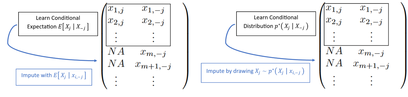
First, there are a myriad of imputation methods with various flavors; the recent benchmark in [7] collects more than 70 methods. We will illustrate a few methods that can easily be accessed in R, referenced in Table LABEL:tab:methods, including a few variations of the famous multiple imputation by chained equations (mice) methodology [28], illustrated in Figure 1. When used to its full potential, it is hard to understate how powerful this iterative approach is. However, the goal of this guide is not necessarily to give a recommendation of what imputation methods to use. Instead, this guide is designed to showcase the aforementioned pitfalls and help applied researchers avoid them. We also present a way to choose the best imputation method for a given task based on [15, näf2025Iscore] and discuss a “challenge” that can be used to assess how well an imputation method might perform.

In the following, we draw heavy inspiration from [näf2025good, näf2025Iscore, 7] in Sections 2 and 3. Then we discuss a few insights about uncertainty quantification with imputation in Section 4. As such, we note that this guide is not free of bias and focuses on issues that we find important in imputation. This might be remedied in new versions of this guide, but will likely not completely vanish. In particular, our guide is centered around iterative imputation as in the mice algorithm, or the well-known knn imputation and focuses on classical i.i.d. tabular data sets of moderate size (i.e. large $n$ small $p$). In such settings at least, it seems the iterative/mice methods perform extremely well, as explored extensively in [7].

Figure 1: Illustration of the mice imputation algorithm, originally from the fantastic video https://www.youtube.com/watch?v=zX-pacwVyvU, recreated and adapted using TikZ. Note that in accordance to Rule 1 in Section 2, the mice algorithm in each step learns a (conditional) distribution of one variable given all the others and depending on what method one chooses (linear regression with Gaussian errors, random forest, etc) a different method emerges.

Problem setup

We try to only use mathematical symbols when they are actually helpful. Figure 2 summarizes our main notation; we assume there is a true underlying matrix $\mathbf{X}$ of dimension $n\times d$ with $n$ i.i.d. observations of vectors in $\mathbb{R}^{d}$. This is the unobserved data following a distribution $P$. What we actually observe is the matrices $\mathbf{M}$, and $\mathbf{X}^{*}$. The latter is the matrix of i.i.d. observations with missing values, arising from masking the observations in $\mathbf{X}$ by $\mathbf{M}$. That is, if $M_{i,j}=0$, then $X^{*}_{i,j}=X_{i,j}$ but if $M_{i,j}=0$, then $X^{*}_{i,j}=\textrm{NA}$, i.e. we do not observe $X_{i,j}$. We can thus observe $\mathbf{M}$ simply by checking with values were not observed (in R for instance, M<- is.na(data) * 1). Each observation (row) in $\mathbf{M}$ thus takes values in $\{0,1\}^{d}$. Each of these possible values is usually called a pattern. For instance, in Figure 2, the first observation has pattern $(0,0,0)$ (fully observed) while the second one has pattern $(1,0,0)$ ($X_{1,2}$ missing). The well-known missingness mechanism–missing completely at random (MCAR), missing at random (MAR) and missing not at random (MNAR)– usually framed in terms of the conditional distribution of $X\mid M$ (see e.g., [13, 22]), can actually be phrased in terms of the following question: “How can distributions change when moving from one pattern to another?”. We will not go into details about this here but refer to [näf2025good].

Figure 2: $\mathbf{X}$ is the assumed underlying full data, $\mathbf{M}$ is the vector of missing indicators and $\mathbf{X}^{*}$ arises when $\mathbf{M}$ is applied to $\mathbf{X}$. Thus each row of $\mathbf{X}$ (or $\mathbf{X}^{*}$) is an observation under a different pattern. Under missing completely at random (MCAR), no change is allowed. Under misisng at Random (MAR), the only constraint is that the distribution of $X_{1},X_{2}\mid X_{3}$ in the third pattern is the same as the unconditional one.

Table 1: List of imputation methods used in this guide. For the mice methods we use the naming convention of the mice R package

	Methods	Languages	Implementations
1	knn [26]	R	bioconductor:impute [9]
2	mice_cart [29]	R	CRAN:mice [27]
3	mice_drf [näf2025good]	R	Git:KrystynaGrzesiak/miceDRF
4	mice_norm [29]	R	CRAN:mice [27]
5	mice_norm_nob [29]	R	CRAN:mice [27]
6	mice_norm_predict [29]	R	CRAN:mice [27]
7	mice_rf [29]	R	CRAN:mice [27]
8	missForest [24]	R	CRAN:missForest [25]

2 The Three Properties of a Great Imputation

We start by loosely stating 3 ideal properties an imputation method should have in our view:

Rule 3

again reveals a certain bias, as our focus lies on the widely-used MAR condition originally introduced in [20]. There are also more recent alternative conditions that have their own merits, see e.g., [19, näf2025good].

Rule 2

might seem self-explanatory, the more flexible a method the more likely it is to adapt to your data at hand. However, as with any estimation process, the more flexible the method, the more data points are required for accurate estimation. For less than say 200 observations a parametric imputation method like mice.norm_nob might be better suited than a fully nonparametric method such as mice_cart. This may also be true when $n$ is larger, but the data is high dimensional, i.e. $d\geq n$. Nonetheless in general, it seems desirable to have a method that is as flexible as possible.

Rule 1

is the most important of the three and it is the source of most pitfalls. We are not completely precise here, but with “distributional” or “stochastic method”, we mean a method that draws imputations from a distribution instead of trying to predict the most likely value. As [29, Chapter 2.6] put it: Imputation is not prediction. In particular, stochastic methods allow for multiple imputation, because several distinct values can be drawn for each imputation. Imputation is thus a distributional estimation task; we do not know the missing values and it does not make sense trying to predict them. Instead, we want to impute such that we most closely reconstruct the original distribution.

Examples

Gaussian Example

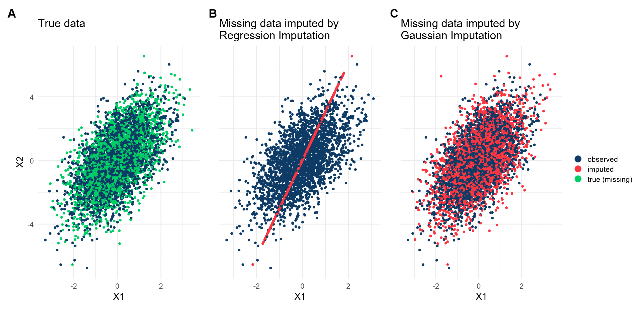
Figure 3 taken from [7] provides an immediate graphical illustration of this issue in a two dimensional Gaussian example. Essentially here we perform the mice algorithm of Figure 1, with two different methods. The imputation on the very right (mice_norm) fits a linear regression of $X_{1}$ onto $X_{2}$ in the pattern where both $X_{1}$ and $X_{2}$ are observed, leading to an estimate $\beta$ for the regression coefficient, and $\sigma^{2}$ for the residual variance. Instead, of directly trying to predict the missing values in the second pattern, using $\beta X_{2}$, the method draws the imputations from the distribution $N(\beta X_{2},\sigma^{2})$. This is also illustrated in Figure 4 on the right. Compared to the the very left picture in Figure 3, we can see that this approach leads to an accurate recreation of the (unobserved) full distribution. Now compare this approach to the one that is often used instead (here represented by mice_norm.predict, but the same would hold true for missForest or knn imputation). Here we try to predict the actual missing values by using $\beta X_{2}$ directly, giving a single value to impute. The detrimental effect of this is immediately visible in the middle picture, where the imputation results in a line through the point cloud. This is not just theoretical; the discrepancy can affect parameter estimation in downstream analyses. For instance, despite the high sample size, regressing $X_{2}$ onto the imputed $X_{1}$ leads to a bias for the regression imputation (estimated value $\approx$ 1.5, true value = 1). On the other hand, the mice_norm_nob imputation leads to an estimated value of $\approx$ 1.03, almost the same value as one obtains using the (unavailable) full data.

Uniform Example

To further illustrate the point, we will now introduce a particularly tricky example that is designed to test if an imputation can truly handle MAR. However, an imputation that imputes by prediction will also fail this test:

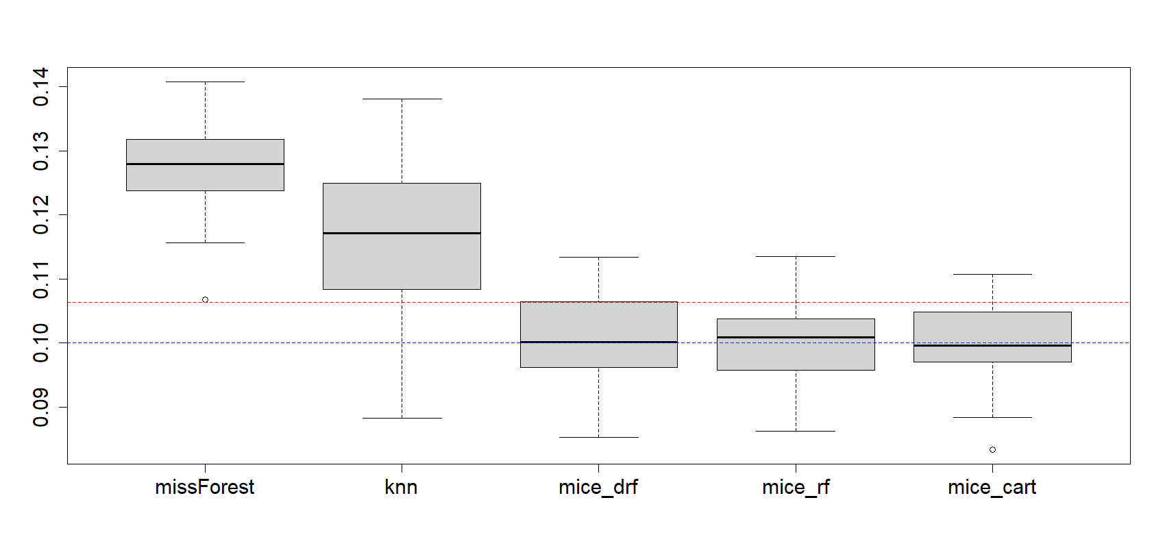
As mentioned this Uniform Example is designed to do two things: First, it will quickly expose methods that do not actually work under MAR, as this is a rather tricky MAR example. Second, methods that do not meet Rule 1 will tend to have an even worse score. Figure 5 showcases the second point for a few selected imputation methods over 50 simulation replications, $n=5000$, and $d=5$ (very low dimensional, but the problem is difficult enough). We note that the blue (lower) line corresponds to the true value of $\alpha=0.1$ (since $X_{1}$ is marginally uniform the desired 0.1 quantile is exactly 0.1). The upper read line instead shows the true (but biased) value we would get if we only estimated the quantile for $X_{1}$ when $X_{1}$ is observed, namely $-7+\sqrt{49+15*0.1}\approx 0.106$.. The first 3 imputation methods, mice_drf, mice_rf, mice_cart, approximately meet Rule 1 and do very well! However, missForest and knn imputation (missForest, knn) that do not meet Rule 1 and try to predict the missing values are over the red line and thus even worse than simply ignoring the missing data. Figure 5 thus shows how trying to do the correct thing, i.e. not ignoring $X_{1}$ when it is missing, with the wrong imputation method, can lead to worse results.

Figure 3: 5000 observations of the bivariate Gaussian Example with around 50% MCAR missing values in $X_{1}$.(A) Original observations (observed and missing), (B) Imputation by fitting a regression model and imputing the prediction (mice_norm.predict), (C) Imputation by fitting a regression model and imputing by drawing from conditional Gaussian distribution (mice_norm). Figure taken from [7].

Figure 4: Imputation by learning from the part where $X_{j}$ is observed and imputing where it is missing, once using prediction (i.e. imputing by the estimated conditional expectation, the most likely value) on the left, and once using stochastic imputation (i.e. by drawing from the actually learned distribution) on the right.

Figure 5: Result of the Uniform Example over 50 simulations, tested on missForest, knn, mice_drf, mice_rf, mice_cart. The vertical line represent the true value (0.1, in blue) and the true quantile of $X_{1}$ when considering only the observed values, without imputation ($-7+\sqrt{49+15*0.1}\approx 0.106$, red). Methods are ordered by how closely the mean over the 50 replications is close to the true value of 0.1. See the file Section_2_QuantileTest.R.

3 How to choose the best Imputation Method

We have seen one way to assess how well an imputation method performs, by using a specifically designed simulated example. Of course this does not necessarily mean that a method that performs well here will also perform well on a given imputation task with a real-world data set, even if the missingness mechanism truly is Missing (Completely) at Random.

As such, confronted with a data set with real missing values (where the true underlying data is not available), one might be tempted to follow the standard approach in practice:

1. delete a few randomly selected values in the data set that were originally observed,

2. impute these artificially removed values, and

3. compare the imputed value(s) to the true observed values using metrics such as RMSE (Root Mean Squared Error) or MAE (Mean Absolute Error).

However, aside from the fact that deleting a value can render a proper MAR mechanism into an MNAR mechanism, this will once again favor methods that try to predict the missing values and violate Rule 1 above. This is because RMSE and MAE are optimized for the expectation and median respectively, so stochastic imputation methods, which introduce additional variance, may appear less attractive.

Imputation Scores

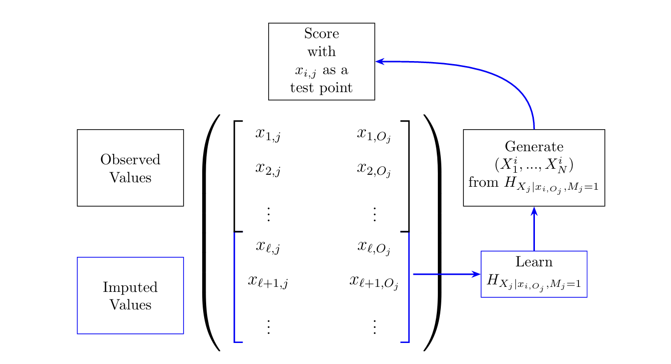
Recently [15, näf2025Iscore] developed scoring methodologies for imputation methods, that should identify the best methods, similar as in the case of prediction. The latest version in [näf2025Iscore], essentially deletes observed values, imputes them and then checks the imputed vs the actually observed values, just as in the standard approach mentioned above. However, instead of using RMSE or MAE to compare one imputed value to one observed value, they impute multiple times, to have several imputed values for each test value. This brings us back to the realm of testing a sample from a predicted distribution (here the $N$ imputations) against a single test point (the previously deleted observed value) and there are convenient so-called proper scores for this [6]. In particular, [näf2025Iscore] use the energy score, thus naming the method “energy-I-Score”. The score is implemented in the package miceDRF. Both the score itself and its implementation are not without its flaws, and the score can take a long time to evaluate. Improving this is a subject of further research.

We illustrate the use of this score in the Uniform Example above. Getting the following result:

mice_drf	mice_rf	mice_cart	missForest	knn
0.1874387	0.1911953	0.2248830	0.2433831	0.2869977

Thus the score puts mice_drf first, followed closely by mice_rf and mice_cart while placing the two methods that violate Rule 1 last. Note that the ordering of the first three methods is reversed compared to Figure 5. This is because their overall performance is very similar, and the score places strong emphasis on correct sampling (i.e. the ability to create multiple imputations). This is a finer point and we will not go into details here – more importantly, choosing the method with the best score (mice_drf) leads to great results in this example.

Figure 6: Illustration of the energy-I-Score, taken from [näf2025Iscore].

4 Uncertainty Quantification

Traditionally, multiple imputation was combined with the so-called Rubin’s rules to generate a variance estimate that would then be used to define confidence intervals for parameters (see e.g., [29]). However, for (non-Bayesian) methods like the methods presented here, Rubin’s rules tend underestimate the variance. This is usually framed as a shortcoming of the imputation method itself and arises from a Bayesian way of thinking where the parameter uncertainty of the imputation model itself is taken into account. As such, while this is a very elegant approach, there are two essential problems:

• Despite the strength of methods such as mice_cart and mice_rf and their ability to produce multiple imputation, using Rubin’s rules might lead to an underestimation of the variance of a parameter and to too short confidence intervals.

• Rubin’s rules are not always straightforward to use, as they require an (asymptotic) expression of the variance of the estimator.

Would it thus be better to not use the powerful mice methods that appear to be some of the few methods achieving good results even in the Uniform Example? We do not think so. Instead, we would like to use an approach that gives reliable (large sample) uncertainty estimation for imputation methods that use distributional imputation as described above.

One possible answer to this is the simple old bootstrap, which in fact was proposed a few times for parametric imputation, see e.g. [21, 8]. In particular, we

• Calculate the main estimator as before, say $\hat{\theta}$, using the original data set (with imputation).

• For $l=1,\ldots,L$ we shuffle the data each time (drawing by replacement), impute and then obtain a slightly different estimator, say $\theta^{*}_{l}$.

• Use the normal approximation to build a confidence interval around $\hat{\theta}$:

  $$\hat{\theta}\pm q_{1-\alpha/2}\cdot\sigma^{*},$$

  where $q_{1-\alpha/2}$ is the $1-\alpha/2$ quantile of a normal distribution (qnorm(1-alpha/2)) and $\sigma^{*}$ is the estimated standard deviation based on the bootstrap samples:

  $$\sigma^{*}=\left(\sum_{l=1}^{L}(\hat{\theta}-\theta^{*}_{l})^{2}\right)^{1/2}.$$

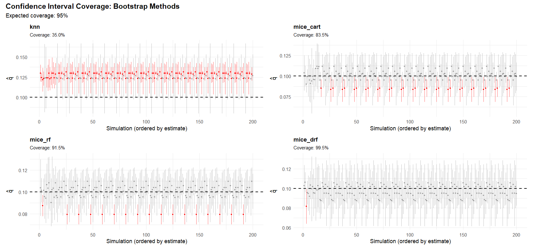
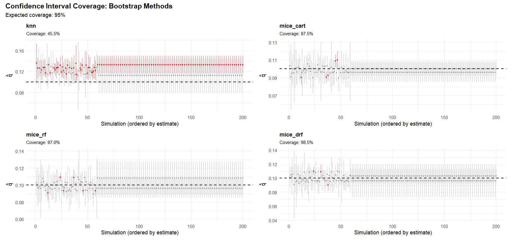
As far as we know, it was not extensively studied with the kind of nonparametric imputation we study here. We apply this procedure on the Uniform Example, this time with $n\in\{1000,2000\}$, but still for $d=5$. We take $L=30$ and impute with knn, mice_drf, mice_rf, mice_cart. missForest is omitted here as it is relatively slow and will result in a very similar performance as knn.

Figure 7 and 8 show the performance of this approach for the four imputation methods. The true value of $0.1$ is shown as the dashed horizontal line and for each of the $B=200$ simulations, a confidence interval is constructed. Ideally, we would like 95% of these intervals to include the true value, while at the same time having intervals that are as short as possible. For the knn imputation, no matter how hard we try to build sensible intervals, its bias is simply too big and as a result it undercovers heavily (the true parameter is inside the confidence interval only 35% and 45.5% respectively). The picture would look almost identical for missForest, again underscoring the inadequacy of methods that fail Rule 1. On the other hand, mice_rf, mice_cart are much better, though they still undercover for $n=1000$. Interestingly, mice_drf, deemed the best method by the energy-I-Score for $n=5000$, has good coverage for $n=1000$, even if the produced intervals are maybe a bit too wide. For $n=2000$ on the other hand, all 3 distributional mice method show the desired coverage. These results might not seem very good given how simple the example is (only $d=5$ and uniform distributions), but we emphasize again that the MAR mechanism here is quite difficult.

Figure 7: Coverage of the true value for the true value of 0.1 for $B=200$ replications, with $L=30$ bootstrap replications each time, $n=1000$, $d=5$. The normality approximation was used to build confidence intervals.

Figure 8: Coverage of the true value for the true value of 0.1 for $B=200$ replications, with $L=30$ bootstrap replications each time, $n=2000$, $d=5$. The normality approximation was used to build confidence intervals.

5 Conclusion

The present paper attempts to give a short and concise, if biased, guide to modern imputation. We discussed that an imputation method should really try to recover the original data distribution (Rule 1), how one might choose a good imputation method in practice, and how to deal with uncertainty quantification.

There are many questions still open, including what theoretical guarantees one actually can achieve and whether there is a more reliable way of uncertainty quantification for smaller samples. However, at least for small to mid-sized data sets, methods such as mice_cart and mice_rf show an incredible ability to recover the true data distribution under MAR.

References

- [1] (2023) An investigation of the imputation techniques for missing values in ordinal data enhancing clustering and classification analysis validity. Decision Analytics Journal 9, pp. 100341. Cited by: §1.
- [2] (2019) Comparison of performance of data imputation methods for numeric dataset. Applied Artificial Intelligence 33 (10), pp. 913–933. Cited by: §1.
- [3] (2024) The performance of prognostic models depended on the choice of missing value imputation algorithm: a simulation study. Journal of Clinical Epidemiology, pp. 111539. Cited by: §1.
- [4] (2023) A simulation study on missing data imputation for dichotomous variables using statistical and machine learning methods. Scientific Reports 13 (1), pp. 9432. Cited by: §1.
- [5] (2023) Performance of multiple imputation using modern machine learning methods in electronic health records data. Epidemiology 34 (2), pp. 206–215. Cited by: §1.
- [6] (2007) Strictly proper scoring rules, prediction, and estimation. Journal of the American Statistical Association 102 (477), pp. 359–378. Cited by: §3.
- [7] (2025) Do we need dozens of methods for real world missing value imputation?. arXiv preprint arXiv:2511.04833. External Links: 2511.04833 Cited by: §1, §1, Figure 3, §2, §3.
- [8] (2024) A unified inference framework for multiple imputation using martingales. Statistica Sinica 34, pp. 1649–1673. Cited by: §4.
- [9] (2024) Impute: impute: imputation for microarray data. Note: R package version 1.80.0 External Links: Link, Document Cited by: Table 1.
- [10] (2021) A benchmark for data imputation methods. Frontiers in big Data 4, pp. 693674. Cited by: §1.
- [11] (2024) On the performance of imputation techniques for missing values on healthcare datasets. arXiv preprint arXiv:2403.14687. Cited by: §1.
- [12] (2019-10-11) Random forest-based imputation outperforms other methods for imputing lc-ms metabolomics data: a comparative study. BMC Bioinformatics 20 (1), pp. 492. Cited by: §1.
- [13] (1986) Statistical analysis with missing data. John Wiley & Sons, Inc.. Cited by: §1.
- [14] (2022) An experimental survey of missing data imputation algorithms. IEEE Transactions on Knowledge and Data Engineering 35 (7), pp. 6630–6650. Cited by: §1.
- [15] (2023) Imputation scores. The Annals of Applied Statistics 17 (3), pp. 2452 – 2472. Cited by: §1, §3.
- [16] (2023) Imputation of missing values for cochlear implant candidate audiometric data and potential applications. Plos one 18 (2), pp. e0281337. Cited by: §1.
- [17] (2024) Imputation of data missing not at random: artificial generation and benchmark analysis. Expert Systems with Applications 249, pp. 123654. Cited by: §1.
- [18] (2018) Missing data imputation for supervised learning. Applied Artificial Intelligence 32 (2), pp. 186–196. Cited by: §1.
- [19] (2023-08) Multiple imputation for non-monotone missing not at random data using the no self-censoring model. Stat Methods Med Res 32 (10), pp. 1973–1993 (en). Cited by: §2.
- [20] (1976) Inference and missing data. Biometrika 63 (3), pp. 581–592. Cited by: §2.
- [21] (2018) Bootstrap inference when using multiple imputation. Statistics in Medicine 37 (14), pp. 2252–2266. Cited by: §4.
- [22] (2013) What is meant by “Missing at Random”?. Statistical Science 28 (2), pp. 257–268. Cited by: §1, footnote 1.
- [23] (2022) An intelligent missing data imputation techniques: a review. JOIV: International Journal on Informatics Visualization 6 (1-2), pp. 278–283. Cited by: §1.
- [24] (2012) MissForest—non-parametric missing value imputation for mixed-type data. Bioinformatics 28 (1), pp. 112–118. Cited by: Table 1.
- [25] (2022) MissForest: nonparametric missing value imputation using random forest. Note: R package version 1.5 Cited by: Table 1.
- [26] (2001) Missing value estimation methods for DNA microarrays. Bioinformatics 17 (6), pp. 520–525. Cited by: Table 1.
- [27] (2023) Mice: multivariate imputation by chained equations. Note: R package version 3.16.0 Cited by: Table 1, Table 1, Table 1, Table 1, Table 1.
- [28] (2011) mice: multivariate imputation by chained equations in R. Journal of Statistical Software 45 (3), pp. 1–67. Cited by: §1.
- [29] (2018) Flexible imputation of missing data. second edition. Vol. , Chapman & Hall/CRC Press. Cited by: Table 1, Table 1, Table 1, Table 1, Table 1, §2, §4.
- [30] (2022) Are deep learning models superior for missing data imputation in surveys? Evidence from an empirical comparison. Survey Methodology 48 (2). Cited by: §1.
- [31] (2023) A comparative study of imputation methods for multivariate ordinal data. Journal of Survey Statistics and Methodology 11 (1), pp. 189–212. Cited by: §1.
- [32] (2018) GAIN: missing data imputation using generative adversarial nets. In Proceedings of the 35th International Conference on Machine Learning, pp. 5689–5698. Cited by: §1.