APEX: Learning Adaptive Priorities for Multi-Objective Alignment in Vision-Language Generation

Abstract

Multi-objective alignment for text-to-image generation is commonly implemented via static linear scalarization, but fixed weights often fail under heterogeneous rewards, leading to optimization imbalance where models overfit high-variance, high-responsiveness objectives (e.g., OCR) while under-optimizing perceptual goals. We identify two mechanistic causes: variance hijacking, where reward dispersion induces implicit reweighting that dominates the normalized training signal, and gradient conflicts, where competing objectives produce opposing update directions and trigger seesaw-like oscillations. We propose APEX (Adaptive Priority-based Efficient X-objective Alignment), which stabilizes heterogeneous rewards with Dual-Stage Adaptive Normalization and dynamically schedules objectives via $\mathcal{P}^{3}$ Adaptive Priorities that combine learning potential, conflict penalty, and progress need. On Stable Diffusion 3.5, APEX achieves improved Pareto trade-offs across four heterogeneous objectives, with balanced gains of +1.31 PickScore, +0.35 DeQA, and +0.53 Aesthetics while maintaining competitive OCR accuracy, mitigating the instability of multi-objective alignment.

APEX: Learning Adaptive Priorities for Multi-Objective Alignment in Vision-Language Generation

Dongliang Chen^,1   Xinlin Zhuang^∗,1   Junjie Xu^∗,1   Luojian Xie¹   Zehui Wang¹ Jiaxi Zhuang¹   Haolin Yang²   Liang Dou¹   Xiao He¹   Xingjiao Wu^,1   Ying Qian^{†,1 1}East China Normal University  ²MBZUAI

1 Introduction

Vision-language generation (Bie et al., 2025) has advanced rapidly in recent years, enabling text-to-image (T2I) models based on diffusion and flow matching to synthesize high-fidelity images from natural language prompts (Ho et al., 2020; Rombach et al., 2022; Lipman et al., 2023; Bie et al., 2025). As these systems move from demos to real use cases, a single notion of quality is no longer sufficient. Practical alignment must simultaneously satisfy heterogeneous objectives, ranging from discrete structural constraints (e.g., rendering legible text) to perceptual preferences (aesthetics, realism, artifact suppression) (Xu et al., 2023; Zhang et al., 2024). However, these objectives are often competing: improving local sharpness to boost text readability can degrade global lighting coherence or introduce artifacts, yielding a brittle “one-metric-at-a-time” behavior (as shown in Figure 1). Therefore, achieving multi-objective alignment in T2I generation is a critical challenge.

Figure 1: Images generated by Stable Diffusion 3.5 under different competing objective settings. For the prompt A city square with a billboard… filled with ’Your Ad Here’, optimizing for text clarity (left) or visual quality (middle) leads to imbalance. APEX achieves effective multi-objective alignment (right).

To optimize black-box, non-differentiable objectives (e.g., OCR metrics and preference models), reinforcement learning (RL) has become a standard paradigm for post-training alignment (Ziegler et al., 2020; Black et al., 2024) In the multi-objective setting, existing approaches typically rely on Static Linear Scalarization, which combines disparate reward signals using fixed weights that remain constant throughout training (Clark et al., 2024). Despite its simplicity, we find that static scalarization fails systematically for heterogeneous rewards, producing severe optimization imbalance that cannot be resolved by merely tuning weights. Our analysis identifies two mechanistic failure modes that explain this behavior. (1) Variance Hijacking. Even with equal preset weights (Figure 2, top-right), objectives with larger dispersion or stronger responsiveness can implicitly dominate the normalized training signal, effectively hijacking the gradient budget. In practice, high-variance, discrete constraints such as OCR can saturate early while continuing to monopolize updates, starving low-variance perceptual objectives and preventing further improvement elsewhere. This makes the intended scalarization weights unreliable as a control mechanism. (2) Gradient Conflicts. Because objectives share parameters, their policy gradients can point in opposing directions. These conflicts appear intermittently and can be severe, causing oscillations, forgetting, and “seesaw” trade-offs where improvements in one objective coincide with regressions in others. Together, variance hijacking and gradient conflicts explain why static scalarization often yields unstable training and poor Pareto trade-offs in T2I alignment.

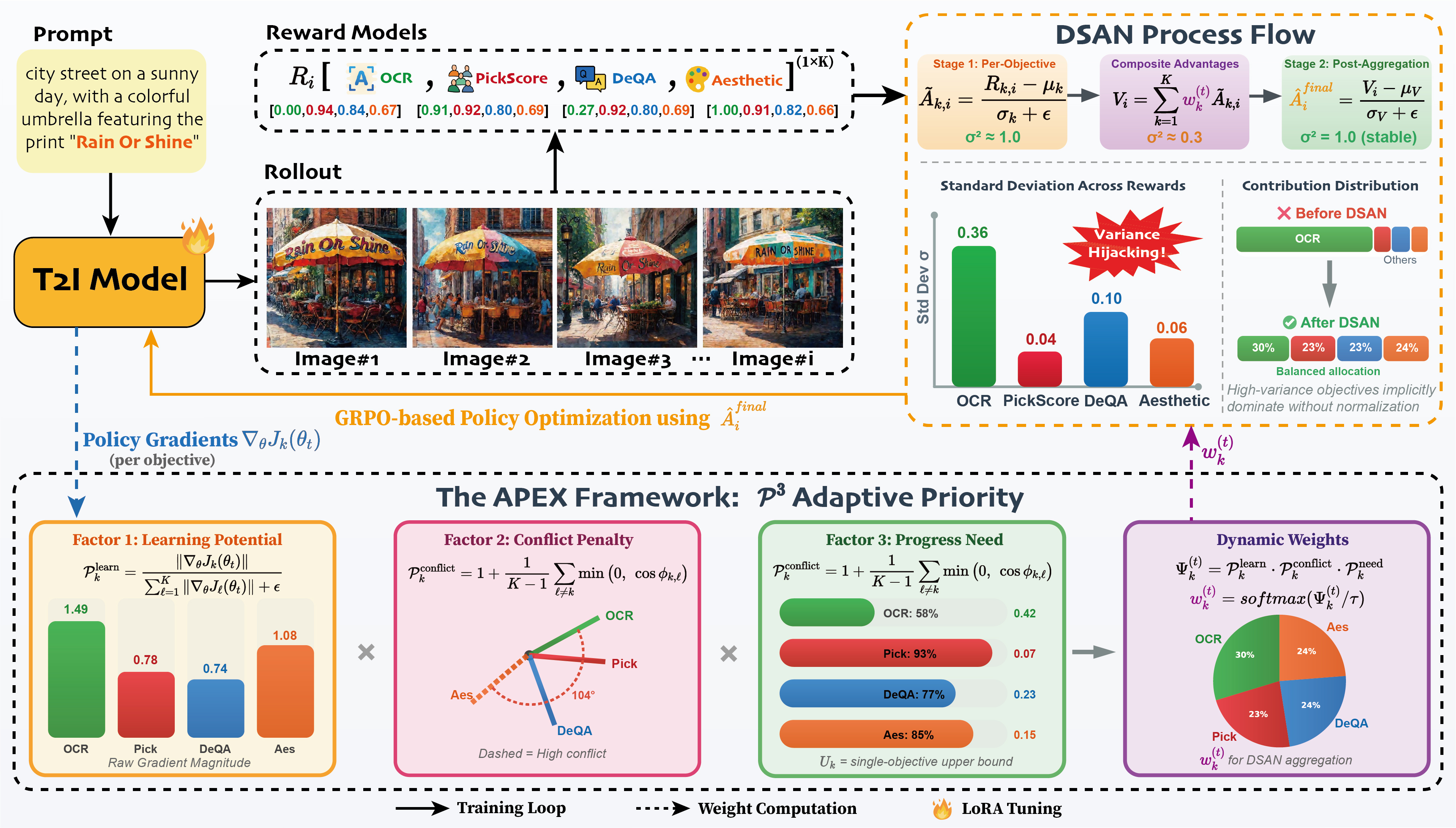
These observations suggest that effective multi-objective alignment requires state-dependent scheduling, adjusting priorities based on training dynamics rather than fixed weights. To this end, we propose APEX (Adaptive Priority-based Efficient X-objective Alignment), a simple yet effective framework that addresses both failure modes without discarding much generated samples (unlike sample-filtering approaches such as Parrot (Lee et al., 2024)). APEX decouples two roles that are conflated in static scalarization: (i) constructing a stable scalar learning signal under heterogeneous rewards, and (ii) deciding which objectives to emphasize at each stage of training. Specifically, APEX introduces Dual-Stage Adaptive Normalization (DSAN) to neutralize variance hijacking by standardizing rewards per objective and re-normalizing after aggregation, keeping the effective update scale stable even as priorities change. On top of this calibrated signal space, the $\bm{\mathcal{P}^{3}}$ mechanism computes adaptive priorities from learning potential, inter-objective conflicts, and remaining headroom to empirical upper bounds, dynamically steering optimization toward bottlenecks while damping destructive interference.

In summary, our contributions are as follows: First, we provide a mechanistic analysis of why static scalarization fails in multi-objective T2I RL, identifying variance hijacking and gradient conflicts as causes of optimization imbalance. Second, we propose APEX, a decoupled framework combining DSAN (stable normalization under heterogeneous rewards) with $\bm{\mathcal{P}^{3}}$ (dynamic priority scheduling from training-state signals). Third, experiments on Stable Diffusion 3.5 demonstrate improved Pareto trade-offs across OCR, Aesthetic, PickScore, and DeQA, achieving substantially higher hypervolume than static scalarization while maintaining full sample efficiency.

2 Related Work

RL for T2I Alignment. As T2I architectures evolve from Latent Diffusion Models (LDMs) (Rombach et al., 2022) to Flow Matching frameworks (Lipman et al., 2023), the research focus has shifted from high-fidelity image synthesis to precise alignment with multi-faceted human intents. Reinforcement Learning (RL) has emerged as the core paradigm for post-training alignment: methods like DPOK (Fan et al., 2023) and DDPO (Black et al., 2024) stabilize training via KL regularization and policy optimization. Human preference benchmarks (Xu et al., 2023; Kirstain et al., 2023) provide unified reward signals; DRaFT (Clark et al., 2024) validated static linear scalarization for multiple rewards. Notably, Flow-GRPO (Liu et al., 2025) successfully extended Group Relative Policy Optimization to flow matching models, improving single-step efficiency. However, these methods remain primarily single-objective driven. In contrast, our APEX mechanism introduces dynamic priority scheduling, extending optimization to complex heterogeneous multi-objective scenarios.

Multi-Objective Optimization. Finding a Pareto-optimal balance between conflicting objectives remains a central challenge. Parrot (Lee et al., 2024) approximates the Pareto front through non-dominated sorting (NSGA-II Deb et al. 2002), but relies on rejection sampling with significant sample wastage. T2I-R1 (Jiang et al., 2025) integrates Chain-of-Thought for semantic planning, yet employs fixed ensemble averaging without dynamic priority allocation. In the LLM domain, Lu et al. (2025) addresses the failure of fixed-weight linear scalarization by introducing dynamic reward weighting. Concurrent work (Lyu et al., 2025) explores independent reward normalization. Inspired by these, APEX addresses unique T2I challenges: cross-modal heterogeneous rewards (e.g., discrete OCR versus smooth aesthetics) cause severe “variance hijacking,” where high-variance signals implicitly dominate optimization. APEX mitigates this through DSAN for signal calibration and a $\bm{\mathcal{P}^{3}}$ priority scheduler that fuses gradient geometry with Utopia Point (Marler and Arora, 2004) metrics to guide toward the Pareto front efficiently.

Figure 2: Overview of the APEX framework. Top: The training loop generates rollouts from prompts, evaluates them with multiple reward models, and performs GRPO-based policy optimization. DSAN eliminates variance hijacking via dual-stage normalization, producing balanced gradient contributions. Bottom: The $\mathcal{P}^{3}$ mechanism analyzes per-objective policy gradients $\nabla_{\theta}J_{k}(\theta_{t})$ (used only for weight computation, not parameter updates) to compute dynamic weights $w_{k}^{(t)}$ by fusing learning potential, conflict penalty, and progress need, which are subsequently fed back to DSAN for advantage aggregation.

3 Method

3.1 Preliminaries

We consider a flow-matching-based text-to-image model parameterized by $\theta$. Given a prompt $c\sim\mathcal{D}$, the model generates an image $x_{0}\in\mathbb{R}^{H\times W\times 3}$ by denoising from an initial latent $x_{1}$ along a continuous time variable $j\in[0,1]$ (with $j=1$ being noise and $j=0$ being data). In practice, we discretize time into $T$ steps $\{j_{t}\}_{t=0}^{T}$ with $j_{0}=0$ and $j_{T}=1$, and denote the discrete trajectory as $\tau=\{x_{j_{T}},x_{j_{T-1}},\dots,x_{j_{0}}\}$.

Standard flow matching inference follows a deterministic reverse-time ODE: $dx_{j}=v_{\theta}(x_{j},j)\,dj$, which is unsuitable for policy-gradient-style alignment due to the lack of stochastic exploration and an explicit tractable transition density. To enable stochastic sampling while preserving the model’s marginal distribution, we adopt the ODE-to-SDE conversion from recent work on stochastic flow matching (Albergo et al., 2023; Liu et al., 2025):

$$\begin{split}dx_{j}&=v_{\theta}(x_{j},j)\,dj\\ &\quad+\frac{\sigma_{j}^{2}}{2j}\left(x_{j}+(1-j)\,v_{\theta}(x_{j},j)\right)dj+\sigma_{j}\,dw,\end{split}$$ (1)

where $w$ is a standard Wiener process and $\sigma_{j}$ controls stochasticity. This SDE is constructed so that its marginal distribution matches the original ODE model under suitable conditions. Details and derivations are provided in Appendix A.

We discretize Eq. (1) using a numerical SDE solver (e.g., Euler–Maruyama), yielding a stochastic Markov chain with Gaussian transitions:

$$\pi_{\theta}(x_{j_{t-1}}\mid x_{j_{t}},c)=\mathcal{N}\!\left(x_{j_{t-1}};\ \mu_{\theta}(x_{j_{t}},j_{t},c),\ \Sigma_{j_{t}}\right).$$ (2)

The closed-form Gaussian density enables tractable computation of (i) per-step log-probabilities $\log\pi_{\theta}(x_{j_{t-1}}\mid x_{j_{t}},c)$, (ii) likelihood ratios used by PPO/GRPO, and (iii) analytical KL divergence to a reference policy $\pi_{\text{ref}}$ (Appendix B).

GRPO for flow matching policies.

To align $\pi_{\theta}$ without training an additional critic, we adopt Group Relative Policy Optimization (GRPO) (Shao et al., 2024). For each prompt $c$, we sample a group of $G$ independent trajectories under the stochastic policy induced by Eq. (2), obtaining images $\{x_{0}^{(i)}\}_{i=1}^{G}$. Let $\theta_{\text{old}}$ be the behavior policy. The per-step likelihood ratio is

$$r_{t}^{(i)}(\theta)=\frac{\pi_{\theta}(x_{j_{t-1}}^{(i)}\mid x_{j_{t}}^{(i)},c)}{\pi_{\theta_{\text{old}}}(x_{j_{t-1}}^{(i)}\mid x_{j_{t}}^{(i)},c)}.$$ (3)

GRPO maximizes a clipped objective, regularized by KL divergence to the reference policy (see Appendix A.3 for the complete formulation).

3.2 Problem Formulation

Given a prompt $c\sim\mathcal{D}$, the policy $\pi_{\theta}$ samples an image $x_{0}\sim\pi_{\theta}(\cdot\mid c)$. We are provided with $K$ heterogeneous reward functions $\{R_{k}(x_{0},c)\}_{k=1}^{K}$ (e.g., text-image faithfulness, aesthetics, OCR quality), and we aim to improve all of them during fine-tuning. Define the expected performance of each objective

$$J_{k}(\theta)\triangleq\mathbb{E}_{c\sim\mathcal{D},\ x_{0}\sim\pi_{\theta}(\cdot\mid c)}\!\left[R_{k}(x_{0},c)\right],$$ (4)

where $k\in\{1,\dots,K\}$. The alignment goal is naturally multi-objective, i.e., to improve the vector $\big[J_{1}(\theta),\dots,J_{K}(\theta)\big]^{\top}$. Since our optimizer operates on a scalar loss, a common practice is to optimize a scalarization of objectives:

$$J(\theta;\mathbf{w})\triangleq\sum_{k=1}^{K}w_{k}\,J_{k}(\theta),$$ (5)

where $\mathbf{w}\in\Delta^{K-1}=\{\mathbf{w}:\ w_{k}\geq 0,\ \sum_{k=1}^{K}w_{k}=1\}$. Equivalently, at the sample level this corresponds to a scalarized reward

$$R(x_{0},c;\mathbf{w})=\sum_{k=1}^{K}w_{k}\,R_{k}(x_{0},c).$$ (6)

All rewards are defined on the final image $x_{0}$ (terminal reward), while the policy is the stochastic reverse-time trajectory induced by Eq. (2).

Why dynamic weights are needed?

Most prior pipelines use a fixed $\mathbf{w}$ throughout training, such as DRaFT (Clark et al., 2024). In practice, a fixed $\mathbf{w}$ does not guarantee balanced progress across objectives because the optimization state changes over time. Concretely, (i) some objectives may currently provide stronger learning signals than others, (ii) objectives can interact through shared parameters and may help or hinder each other, and (iii) some objectives may plateau earlier and benefit less from continued emphasis. These effects evolve during fine-tuning, motivating a state-dependent weighting rule $\mathbf{w}^{(t)}$ that adapts to the current training dynamics, where $t$ denotes the training step index.

Under GRPO, a direct instantiation plugs the scalarized reward in Eq. (6) into group-relative advantage normalization:

$$\begin{split}R^{(i)}&=\sum_{k=1}^{K}w_{k}^{(t)}\,R_{k}(x_{0}^{(i)},c),\\ \hat{A}^{(i)}&=\frac{R^{(i)}-\text{mean}(\{R^{(m)}\}_{m=1}^{G})}{\text{std}(\{R^{(m)}\}_{m=1}^{G})+\epsilon}.\end{split}$$ (7)

While simple, this weight-then-normalize baseline can be unstable under heterogeneous rewards and time-varying weights: objectives with larger dispersion can disproportionately shape the normalized advantage, and changing $\mathbf{w}^{(t)}$ can shift the advantage statistics and effectively rescale the update from one iteration to the next. This motivates (i) an advantage construction that is robust to reward heterogeneity, and (ii) a principled mechanism for updating $\mathbf{w}^{(t)}$ from the observed optimization state.

3.3 The APEX Method

We propose APEX, a dynamic multi-objective alignment method built on GRPO. APEX is designed as a two-level solution that jointly stabilizes the training signal and adapts the objective priorities: (i) Dual-Stage Adaptive Normalization (DSAN) constructs a scalar advantage whose scale is stable under heterogeneous rewards and changing weights, and (ii) the $\bm{\mathcal{P}^{3}}$ mechanism updates weights from the current learning signal strength, inter-objective interaction, and remaining improvement room. Together, DSAN and $\bm{\mathcal{P}^{3}}$ form a closed loop: $\bm{\mathcal{P}^{3}}$ adjusts what to emphasize, while DSAN ensures the resulting scalar advantage remains comparable across iterations and does not inadvertently change the effective update strength. An overview of APEX is provided in Figure 2.

3.3.1 Dual-Stage Adaptive Normalization

Stage 1. Per-objective group standardization.

For each objective $k$, we compute a group-relative standardized advantage:

$$\tilde{A}_{k}^{(i)}=\frac{R_{k}(x_{0}^{(i)},c)-\text{mean}(\{R_{k}(x_{0}^{(m)},c)\}_{m=1}^{G})}{\text{std}(\{R_{k}(x_{0}^{(m)},c)\}_{m=1}^{G})+\epsilon},$$ (8)

where $\epsilon$ is a small constant for numerical stability. This aligns objectives onto a comparable scale so that no single reward dominates the update merely due to scale or dispersion.

Stage 2. Post-aggregation normalization.

Given weights $\mathbf{w}^{(t)}$, we aggregate standardized advantages and normalize again:

$$\begin{split}V^{(i)}&=\sum_{k=1}^{K}w_{k}^{(t)}\,\tilde{A}_{k}^{(i)},\\ \hat{A}_{\text{final}}^{(i)}&=\frac{V^{(i)}-\text{mean}(\{V^{(m)}\}_{m=1}^{G})}{\text{std}(\{V^{(m)}\}_{m=1}^{G})+\epsilon}.\end{split}$$ (9)

Stage 2 makes the overall advantage distribution stable even when $\mathbf{w}^{(t)}$ changes, preventing inadvertent iteration-to-iteration rescaling of the effective GRPO update. Empirical evidence of advantage variance dynamics is provided in Appendix D.4.

3.3.2 $\bm{\mathcal{P}^{3}}$ Adaptive Priority Mechanism

APEX assigns each objective $k$ a priority score $\Psi_{k}^{(t)}$ and maps priorities to weights through softmax:

$$\begin{split}\Psi_{k}^{(t)}&=\mathcal{P}^{\text{learn}}_{k}\cdot\mathcal{P}^{\text{conflict}}_{k}\cdot\mathcal{P}^{\text{need}}_{k},\\ w_{k}^{(t)}&=\frac{\exp(\Psi_{k}^{(t)}/\tau)}{\sum_{\ell=1}^{K}\exp(\Psi_{\ell}^{(t)}/\tau)}.\end{split}$$ (10)

$\mathcal{P}^{3}$is motivated from the local dynamics of optimizing the scalarized objective $J(\theta;\mathbf{w})=$ $\sum_{k}w_{k}J_{k}(\theta)$. The multiplicative aggregation follows non-compensatory selection principles in multi-criteria optimization (Marler and Arora, 2004) (derivation in Appendix C.1). A gradient step gives $\Delta\theta\propto$ $\sum_{\ell}w_{\ell}\nabla J_{\ell}$, and the first-order change of objective $k$ is

$$\begin{split}\Delta J_{k}&\approx\nabla J_{k}^{\top}\Delta\theta\\ &=\eta\sum_{\ell=1}^{K}w_{\ell}\ \nabla J_{k}^{\top}\nabla J_{\ell}\\ &=\eta\bigg(w_{k}\|\nabla J_{k}\|^{2}\\ &\quad+\sum_{\ell\neq k}w_{\ell}\|\nabla J_{k}\|\,\|\nabla J_{\ell}\|\cos\phi_{k,\ell}\bigg).\end{split}$$ (11)

Eq. (11) suggests using (i) gradient magnitude as a learning-signal strength proxy and (ii) cosine similarity as an inter-objective interaction (synergy/conflict) proxy. Since this local approximation does not reflect long-term objective saturation, we further introduce a progress need signal based on distance to an empirical upper bound.

Learning potential (LP).

We define

$$\mathcal{P}^{\text{learn}}_{k}=\frac{\|\nabla_{\theta}J_{k}(\theta_{t})\|}{\sum_{\ell=1}^{K}\|\nabla_{\theta}J_{\ell}(\theta_{t})\|+\epsilon},$$ (12)

where $\epsilon$ is a small constant (set to $10^{-8}$) for numerical stability, preventing division by zero. Gradient estimation details are provided in Appendix D.1.

Conflict penalty (CP).

We penalize objectives that conflict with others:

$$\begin{split}\mathcal{P}^{\text{conflict}}_{k}&=1+\frac{1}{K-1}\sum_{\ell\neq k}\min\big(0,\ \cos\phi_{k,\ell}\big),\\[2.0pt] \cos\phi_{k,\ell}&=\frac{\langle\nabla J_{k},\nabla J_{\ell}\rangle}{\|\nabla J_{k}\|\,\|\nabla J_{\ell}\|+\epsilon}.\end{split}$$ (13)

Progress need (PN).

Let $U_{k}$ be an empirical upper bound (utopia point) and $\bar{R}_{k}^{(t)}$ be a running performance estimate. We define

$$\mathcal{P}^{\text{need}}_{k}=1+\max\Big(0,\ \frac{U_{k}-\bar{R}_{k}^{(t)}}{U_{k}+\epsilon}\Big).$$ (14)

Estimation details for $U_{k}$ and $\bar{R}_{k}^{(t)}$ are provided in Appendix D.1, enabling bottleneck identification.

Default Settings.

The ${\mathcal{P}^{3}}$ mechanism is designed for adaptive scheduling rather than monotonic convergence. It possesses formal stability guarantees: softmax normalization ensures weights never vanish or concentrate on a single objective, with weight ratios bounded by $\exp(2/\tau)$ (Appendix C for proofs).

Unless otherwise stated, we set $\tau=1$. Putting everything together, APEX replaces the naive advantage in Eq. (7) with DSAN (Eqs. (8)–(9)) and updates weights using $\bm{\mathcal{P}^{3}}$ (Eq. (10)).

Model	Text Rendering	Human Pref.	Image Quality		Hypervolume
	OCR Acc. ($\uparrow$)	PickScore ($\uparrow$)	DeQA ($\uparrow$)	Aesthetic ($\uparrow$)	($\uparrow$)
Base Model
SD3.5-M	0.59	21.72	4.07	5.39	-
Single-Objective Specialists
Flow-GRPO (OCR-Only)	0.92	22.44	4.06	5.32	0.00
Flow-GRPO (PickScore-Only)	0.69	23.53	4.22	5.92	1.11
Multi-Objective Generalists
Flow-GRPO (Static-Weight)	0.88	22.62	4.24	5.51	0.41
APEX (Ours)	0.83	23.03	4.42	5.92	4.49

Table 1: Main Results. Performance comparison on text rendering (evaluated on OCR test set), as well as human preference and image quality (both evaluated on DrawBench). Hypervolume approximates each model’s Pareto contribution as the product of normalized improvements over the base model (SD3.5-M). Metrics are normalized for HV computation: OCR$\in[0,1]$ (inherently scaled), PickScore/26, DeQA/5, Aesthetic/10 (see Appendix D.2). Bold indicates the best performance across all models (ties included), while underline marks the best within the multi-objective group when it differs from the global best.

4 Experiment

We evaluate APEX on Stable Diffusion 3.5 Medium (SD3.5-m) (Esser et al., 2024) across four heterogeneous objectives to answer: (i) Does APEX improve Pareto trade-offs over static weighting? (ii) How does APEX resolve variance hijacking and gradient conflicts? (iii) Are DSAN and $\mathcal{P}^{3}$ both necessary? Section 4.1 describes experimental setup; Section 4.2 presents main results; Section 4.3 analyzes training dynamics; Section 4.4 validates each component via ablation studies.

4.1 Experimental Setup

Objectives.

Four heterogeneous reward functions are selected, spanning from structural constraints to perceptual qualities: (1) OCR (Saharia et al., 2022): measuring text fidelity via normalized Levenshtein distance, representing discrete structural constraints with high variance; (2) PickScore (Kirstain et al., 2023): human preference model for image-text alignment trained on large-scale feedback; (3) DeQA (You et al., 2025): multi-modal LLM-based metric quantifying distortions and low-level artifacts; (4) Aesthetic Score (Schuhmann et al., 2022): CLIP-based regressor for aesthetic appeal. OCR is evaluated on the Flow-GRPO test set (Liu et al., 2025), while others use DrawBench (Saharia et al., 2022).

Baselines.

We compare APEX against Static Linear Scalarization, the standard approach using equal fixed weights ($w_{i}{=}1/K$), a common baseline isolating the effect of dynamic weighting. Single-Objective Specialists (optimized for individual rewards) are reported as performance bounds.

Implementation Details.

We utilize LoRA (Hu et al., 2022) for efficient fine-tuning with GRPO (Shao et al., 2024) adapted for flow matching to enable fast training on 8x NVIDIA A100 GPUs. Training employs 10 denoising steps (vs. 40 for inference) for efficiency. Key hyperparamters are: group size $G{=}24$, learning rate $3{\times}10^{-4}$, temperature $\tau{=}1$. We report single-run results following standard practice (Black et al., 2024; Clark et al., 2024). See Appendix D.1 for full details.

4.2 Main Results

4.2.1 Quantitative Evaluation

Table 1 compares APEX against baselines across four objectives. We report the un-tuned SD3.5-M (Base) model and Single-Objective Specialists to establish performance bounds.

Limitations of Single-Objective Optimization. Specialists achieve peak performance in their target domains at the cost of other objectives. The OCR-Only model’s aesthetic score (5.32) and DeQA (4.06) both fall below the base model; such regressions yield zero hypervolume despite substantial OCR gains. This confirms that single-objective RL causes excessive optimization of discrete structural constraints while sacrificing perceptual quality.

Variance Hijacking in Static Weighting. The static baseline exhibits optimization imbalance. Although reaching OCR accuracy of 0.88, its gains in PickScore (+0.90 over base) and DeQA (+0.17) lag behind APEX (+1.31 and +0.35 respectively), while its aesthetic score (5.51) shows minimal improvement. This supports: without scale calibration, high-variance OCR signals implicitly “hijack” the optimization trajectory, starving low-variance objectives of gradient budget.

Pareto Advancement via APEX. APEX achieves superior multi-objective balance through DSAN and $\mathcal{P}^{3}$. While maintaining competitive OCR (0.83 vs. 0.88 for static weighting), APEX substantially improves perceptual objectives: PickScore reaches 23.03 (98% of the specialist), DeQA achieves 4.42 (highest among all models), and Aesthetic attains 5.92 (tied for best). This demonstrates that adaptive scheduling enables near-specialist performance on individual metrics without sacrificing multi-objective balance. APEX’s hypervolume ($4.49{\times}10^{-5}$, 10.9$\times$ static weighting) quantifies this Pareto dominance (Appendix D.2).

4.2.2 Qualitative Validation

Visual comparisons (Figure 6, Appendix D.3) validate the quantitative findings. APEX demonstrates improved coordination of text rendering, semantic coherence, and visual context, addressing failure modes such as spelling errors and style inconsistencies that occasionally appear in Static-Weight generations. In perceptual quality, APEX shows enhanced lighting modeling, color interaction, and physical plausibility, while Static-Weight exhibits more limited gains over the base model in these fine-grained aesthetic dimensions.

4.3 Analysis of Training Dynamics

We analyze training dynamics to reveal why static scalarization fails and how APEX achieves adaptive multi-objective scheduling.

Figure 3: Training dynamics revealing variance hijacking. Four subplots track four reward objectives across training steps, comparing APEX (blue) and Static-Weight baseline (red). The baseline shows OCR plateauing while Aesthetic stagnates, whereas APEX achieves balanced growth across all dimensions.

Revealing the Pathology of Variance Hijacking.

By comparing the training trajectories of APEX and the Static-Weight baseline (Fig. 3), we demonstrate the variance hijacking phenomenon. In the static baseline, OCR accuracy plateaus near $\sim$0.88 while normalized Aesthetic Score stagnates at $\sim$0.54 throughout training. Even after OCR plateaus, other objectives (image quality, human preference) fail to improve, indicating that high-variance OCR signals continue to dominate gradient updates, leaving low-variance objectives under-optimized. In contrast, APEX achieves synchronized growth across all dimensions through DSAN’s dual-stage normalization; Stage 2 renormalization is verified by variance decay analysis in Appendix D.4.

Figure 4: Analysis of $\bm{\mathcal{P}^{3}}$ dynamics and Hypervolume progression. (a–c) The three $\mathcal{P}^{3}$ factors—Learning Potential, Progress Need, and Conflict Penalty—which jointly guide adaptive weight scheduling. (d) Cumulative Hypervolume comparison showing APEX achieves 3.2$\times$ the dominated space volume of the static baseline.

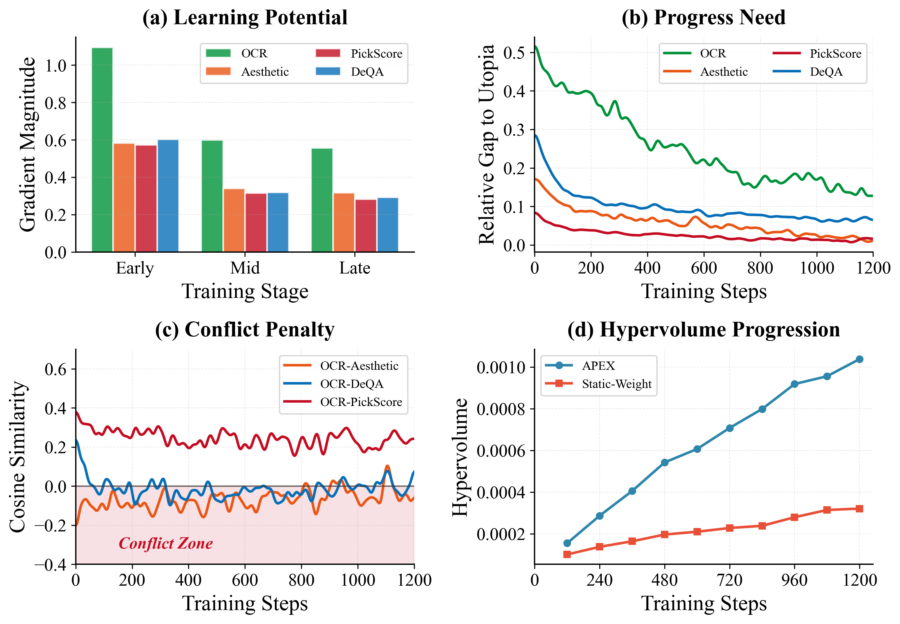
Observations on the $\bm{\mathcal{P}^{3}}$ Mechanism. We deconstruct how the three $\mathcal{P}^{3}$ factors jointly guide adaptive scheduling (Figure 4a-c). The LP factor tracks gradient magnitudes: OCR consistently exhibits high gradient norms, reflecting strong parameter sensitivity, and LP accordingly assigns higher base priority. The PN factor complements this by monitoring distance to empirical upper bounds (Utopia Points); objectives far from saturation receive additional emphasis, redirecting optimization toward bottleneck dimensions with maximal improvement potential. The CP factor addresses a distinct challenge: gradient conflicts exhibit “bursty” behavior, with intermittent severe negative correlations between objectives. CP acts as a dynamic shock absorber, detecting these conflict episodes and temporarily downweighting interfering objectives to prevent destructive gradient interference. Together, these three factors allow APEX to balance exploitation (LP), exploration of underperforming dimensions (PN), and conflict avoidance (CP).

Overall Capability Boundary Analysis. Finally, we quantify overall optimization effectiveness using the Hypervolume (HV) metric (Figure 4d), which measures the volume of objective space dominated by a model’s Pareto set. We evaluate 10 evenly-spaced checkpoints on a held-out test set, using early-training performance as the reference point (see Appendix D.2 for details). The static baseline’s hypervolume growth decelerates significantly in later stages (final HV $\approx 0.0003$), confirming its inability to escape the performance ceiling imposed by variance hijacking. In contrast, APEX maintains robust growth throughout training, ultimately achieving 3.2$\times$ the baseline’s hypervolume (HV $\approx 0.0010$). This 3.2$\times$ improvement demonstrates that APEX successfully expands the Pareto frontier, improving perceptual objectives without sacrificing OCR capability.

4.4 Ablation Studies

Figure 5: Ablation study on DSAN. Reward trajectories over the first 400 steps, comparing APEX Full, APEX w/o DSAN, and Static-Weight. Removing DSAN degrades convergence due to variance hijacking, yet the $\mathcal{P}^{3}$ mechanism still outperforms static weighting. This confirms that DSAN is essential for the adaptive priority mechanism to reach peak performance.

To verify the necessity of each component in APEX, we conduct two sets of ablation experiments: (1) removing DSAN to validate the scale calibration module, and (2) individually ablating each $\mathcal{P}^{3}$ factor to quantify their contributions. Due to computational constraints, we focus on early-to-mid training dynamics where component effects are most pronounced; extended stability analysis is provided in Appendix D.5.

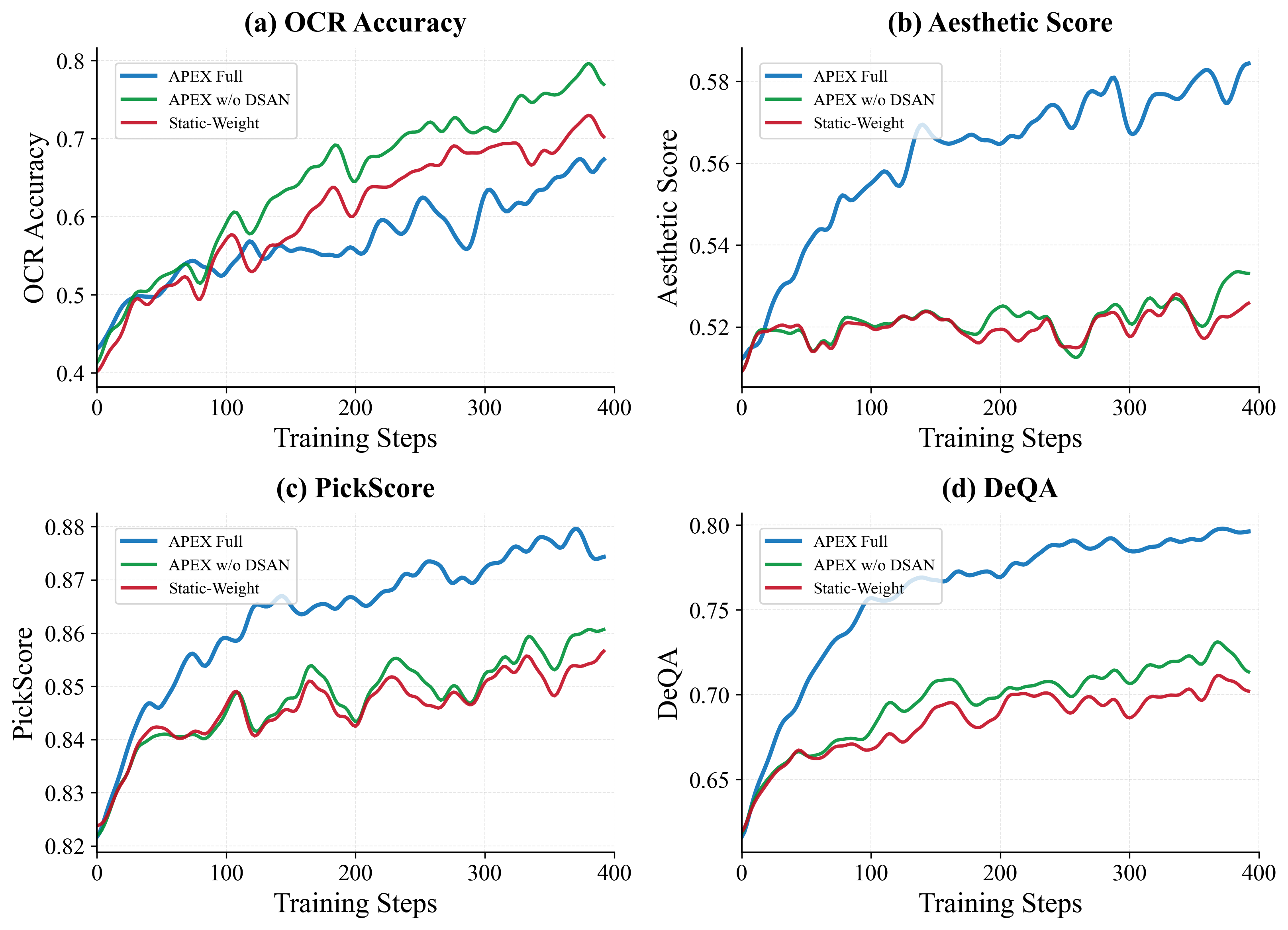
Necessity of Scale Calibration (DSAN). We compare APEX with a variant removing DSAN (APEX w/o DSAN). Figure 5 shows that both w/o DSAN and Static-Weight suffer from variance hijacking: perceptual objectives (Aesthetic, PickScore, DeQA in subplots b-d) stagnate throughout training. However, w/o DSAN consistently outperforms Static-Weight across all objectives (Figure 5), with the most pronounced improvement in OCR (subplot a). This suggests that $\mathcal{P}^{3}$ improves weight allocation even without scale calibration. Yet APEX Full substantially outperforms w/o DSAN across all perceptual dimensions. This confirms that while $\mathcal{P}^{3}$ provides incremental benefits independently, DSAN is essential to fully overcome variance hijacking and unlock the full potential of adaptive multi-objective scheduling.

Variant	Cumulative HV	$\Delta$ vs Full
APEX	$4.26\times 10^{-4}$	—
w/o LP	$3.73\times 10^{-4}$	$-12.5\%$
w/o CP	$3.65\times 10^{-4}$	$-14.5\%$
w/o PN	$3.82\times 10^{-4}$	$-10.3\%$

Table 2: $\bm{\mathcal{P}^{3}}$ Factor Ablation. Cumulative Hypervolume computed over training rewards (50-step averaging window) up to step 600 (see Appendix D.2 for details). Removing any factor leads to 10–15% degradation, with conflict penalty (CP) showing the largest impact.

Contribution of $\bm{\mathcal{P}^{3}}$ Factors. Table 2 presents cumulative Hypervolume when individually removing each factor. Conflict penalty (CP) has the largest impact: removing it causes $-14.5\%$ degradation, as competing gradient directions trigger oscillations without CP’s damping effect. Learning potential (LP) ablation leads to $-12.5\%$ drop, demonstrating the importance of gradient-based priority scheduling. Progress need (PN) removal results in $-10.3\%$ degradation, showing that monitoring distance to upper bounds prevents premature saturation. The comparable magnitudes (10–15%) indicate all three factors are necessary, addressing a distinct aspect of multi-objective optimization.

5 Conclusion

In this paper, we introduce APEX to address optimization imbalance in multi-objective vision-language alignment, where heterogeneous rewards cause overfit to high-variance objectives. Our analysis identified two root causes: variance hijacking, where high-variance objectives dominate gradient updates, and gradient conflicts between competing directions. APEX resolves these through Dual-Stage Adaptive Normalization (DSAN) and $\mathcal{P}^{3}$ Adaptive Priorities. On Stable Diffusion 3.5, APEX achieves 10.9$\times$ the hypervolume of static scalarization with balanced improvements (+1.31 PickScore, +0.35 DeQA, +0.53 Aesthetics) while maintaining competitive OCR, providing a principled framework for multi-objective alignment.

Limitations

Despite its effectiveness, APEX has several limitations that warrant future investigation. APEX requires gradient estimation for priority computation. While manageable, this overhead scales with the number of objectives. Moreover, constrained by computational resources, our validation is limited to SD3.5-Medium. Our future work will explore generalizing APEX across diverse architectures (SDXL, Flux) and modalities (video, audio), as well as to LLM alignment tasks, which face similar multi-objective optimization challenges.

Appendix A Stochastic Flow Matching and GRPO Formulation

For completeness, we provide the derivation of the SDE formulation in Section 3.1, following Albergo et al. (2023); Liu et al. (2025). We adapt the notation to our multi-objective framework.

A.1 From ODE to SDE

Standard flow matching models use a deterministic ODE for generation: $dx_{j}=v_{\theta}(x_{j},j)dj$, where $x_{j}=(1-j)x_{0}+jx_{1}$ with $x_{0}\sim\mathcal{X}_{0}$ (data) and $x_{1}\sim\mathcal{N}(0,I)$ (noise). To enable stochastic sampling, we construct an SDE with matching marginal distributions.

Consider a forward SDE:

$$\begin{split}dx_{j}=\big[v_{\theta}(x_{j},j)+\tfrac{\sigma_{j}^{2}}{2}\nabla\log p_{j}(x_{j})\big]dj\\ +\sigma_{j}dw,\end{split}$$ (15)

where $\sigma_{j}$ controls stochasticity. By the Fokker-Planck equation (Øksendal, 2003), this SDE preserves the ODE’s marginal density $p_{j}(x)$.

Reverse-time SDE.

Applying the standard time-reversal formula (Anderson, 1982):

$$\begin{split}dx_{j}=\big[v_{\theta}(x_{j},j)-\tfrac{\sigma_{j}^{2}}{2}\nabla\log p_{j}(x_{j})\big]dj\\ +\sigma_{j}dw.\end{split}$$ (16)

Score function for rectified flow.

For the linear interpolation $x_{j}=(1-j)x_{0}+jx_{1}$, the conditional score is $\nabla\log p_{j|0}(x_{j}|x_{0})=-x_{1}/j$. The marginal score is:

$$\nabla\log p_{j}(x_{j})=-\tfrac{1}{j}\mathbb{E}[x_{1}|x_{j}].$$ (17)

From the velocity field definition $v_{\theta}(x_{j},j)=\mathbb{E}[x_{1}-x_{0}|x_{j}]$ and the interpolation relation, we derive:

$$\mathbb{E}[x_{1}|x_{j}]=(1-j)v_{\theta}(x_{j},j)+x_{j}.$$ (18)

Substituting Eq. (18) into Eq. (17):

$$\begin{split}\nabla\log p_{j}(x_{j})=-\tfrac{x_{j}}{j}-\tfrac{1-j}{j}v_{\theta}(x_{j},j).\end{split}$$ (19)

Final SDE form.

Plugging this into Eq. (16):

$$\begin{split}dx_{j}&=v_{\theta}(x_{j},j)dj\\ &\quad+\tfrac{\sigma_{j}^{2}}{2j}\big(x_{j}+(1-j)v_{\theta}(x_{j},j)\big)dj\\ &\quad+\sigma_{j}dw,\end{split}$$ (20)

which is Eq. (1) in the main text.

A.2 Euler-Maruyama Discretization

Discretizing Eq. (20) with time step $\Delta j=j_{t-1}-j_{t}<0$:

$$\begin{split}x_{j_{t-1}}&=x_{j_{t}}+\big[v_{\theta}(x_{j_{t}},j_{t})\\ &\quad+\tfrac{\sigma_{j_{t}}^{2}}{2j_{t}}(x_{j_{t}}+(1-j_{t})v_{\theta}(x_{j_{t}},j_{t}))\big]\Delta j\\ &\quad+\sigma_{j_{t}}\sqrt{|\Delta j|}\,\epsilon,\end{split}$$ (21)

where $\epsilon\sim\mathcal{N}(0,I)$. This yields the Gaussian transition in Eq. (2):

$$\pi_{\theta}(x_{j_{t-1}}|x_{j_{t}},c)=\mathcal{N}(x_{j_{t-1}};\mu_{\theta},\Sigma_{j_{t}}),$$ (22)

with

$$\mu_{\theta} =x_{j_{t}}+\big[v_{\theta}(x_{j_{t}},j_{t})$$

$$\quad+\tfrac{\sigma_{j_{t}}^{2}}{2j_{t}}(x_{j_{t}}+(1-j_{t})v_{\theta}(x_{j_{t}},j_{t}))\big]\Delta j,$$ (23)

$$\Sigma_{j_{t}} =\sigma_{j_{t}}^{2}|\Delta j|\cdot I.$$ (24)

Following Liu et al. (2025), we use $\sigma_{j}=a\sqrt{j/(1-j)}$ with $a=0.7$. The Gaussian form enables tractable computation of log-probabilities and likelihood ratios used by GRPO (formulated below).

A.3 GRPO Objective for Flow Matching

Building on the Gaussian transition in Eq. (2), GRPO optimizes:

$$\begin{split}\mathcal{J}_{\text{GRPO}}(\theta)=\mathbb{E}_{c\sim\mathcal{D}}\bigg[&\frac{1}{G}\sum_{i=1}^{G}\bigg(\frac{1}{T}\sum_{t=0}^{T-1}\\ &\min\big(r_{t}^{(i)}\hat{A}^{(i)},\\ &\quad\text{clip}(r_{t}^{(i)},1-\epsilon,1+\epsilon)\hat{A}^{(i)}\big)\\ &-\beta D_{\text{KL}}(\pi_{\theta}\|\pi_{\theta_{\text{old}}})\bigg)\bigg],\end{split}$$ (25)

where $r_{t}^{(i)}$ is the likelihood ratio (Eq. 3), $\hat{A}^{(i)}$ is the group-relative advantage, and $D_{\text{KL}}$ is the trajectory-level KL divergence (see Appendix B for analytical computation).

Appendix B KL Divergence Computation

This appendix provides (i) the analytical form of the KL divergence between Gaussian policies used in our GRPO objective, and (ii) explicit expressions for the discretization scheme referenced in Section 3.1.

B.1 KL Divergence for Gaussian Policies

Given two Gaussian transition policies $\pi_{\theta}$ and $\pi_{\text{ref}}$ with distributions

$$\pi_{\theta}(x_{j_{t-1}}|x_{j_{t}},c) =\mathcal{N}(x_{j_{t-1}};\mu_{\theta},\Sigma_{j_{t}}),$$ (26)

$$\pi_{\text{ref}}(x_{j_{t-1}}|x_{j_{t}},c) =\mathcal{N}(x_{j_{t-1}};\mu_{\text{ref}},\Sigma_{j_{t}}),$$ (27)

the per-step KL divergence has a closed form. Since both policies share the same covariance $\Sigma_{j_{t}}=\sigma_{j_{t}}^{2}|\Delta j|\cdot I$ (as derived in Appendix A), the KL divergence simplifies to:

$$\begin{split}D_{\text{KL}}(\pi_{\theta}\|\pi_{\text{ref}})&=\mathbb{E}_{x_{j_{t-1}}\sim\pi_{\theta}}\left[\log\frac{\pi_{\theta}}{\pi_{\text{ref}}}\right]\\ &=\frac{1}{2\sigma_{j_{t}}^{2}|\Delta j|}\|\mu_{\theta}-\mu_{\text{ref}}\|^{2}.\end{split}$$ (28)

Substituting the mean expressions from Eq. (23) in Appendix A:

$$\begin{split}D_{\text{KL}}(\pi_{\theta}\|\pi_{\text{ref}})&=\frac{(\Delta j)^{2}}{2\sigma_{j_{t}}^{2}|\Delta j|}\Big\|v_{\theta}(x_{j_{t}},j_{t})\\ &\quad+\tfrac{\sigma_{j_{t}}^{2}}{2j_{t}}\big(x_{j_{t}}+(1-j_{t})v_{\theta}\big)\\ &\quad-v_{\text{ref}}(x_{j_{t}},j_{t})\\ &\quad-\tfrac{\sigma_{j_{t}}^{2}}{2j_{t}}\big(x_{j_{t}}+(1-j_{t})v_{\text{ref}}\big)\Big\|^{2}\\ &=\frac{|\Delta j|}{2\sigma_{j_{t}}^{2}}\Big\|\big(1+\tfrac{\sigma_{j_{t}}^{2}(1-j_{t})}{2j_{t}}\big)\\ &\quad\times(v_{\theta}-v_{\text{ref}})\Big\|^{2}.\end{split}$$ (29)

For our noise schedule $\sigma_{j}=a\sqrt{j/(1-j)}$ with $a=0.7$, and uniform time grid $\Delta j=-1/T$, Eq. (29) provides an efficient way to compute the KL penalty in the GRPO objective without expensive Monte Carlo estimation.

Trajectory-level KL.

The trajectory-level KL divergence is:

$$D_{\text{KL}}(\pi_{\theta}(\tau|c)\|\pi_{\text{ref}}(\tau|c))$$

$$=\sum_{t=0}^{T-1}D_{\text{KL}}(\pi_{\theta}(x_{j_{t-1}}|x_{j_{t}},c)\|\pi_{\text{ref}}(x_{j_{t-1}}|x_{j_{t}},c)).$$ (30)

B.2 Discretization Scheme Details

As mentioned in Section 3.1, we discretize the SDE (Eq. 1) using the Euler-Maruyama method. The mean and covariance of the resulting Gaussian transition (Eq. 2) are given by Eqs. (23) and (24) in Appendix A.

Time grid.

We use a uniform grid with $T$ steps: $j_{t}=t/T$ for $t=0,1,\ldots,T$, yielding constant step size $\Delta j=j_{t-1}-j_{t}=-1/T$ (negative for the reverse process).

Log-probability computation.

The per-step log-probability is:

$$\begin{split}\log\pi_{\theta}(x_{j_{t-1}}|x_{j_{t}},c)&=-\tfrac{d}{2}\log(2\pi\sigma_{j_{t}}^{2}|\Delta j|)\\ &\quad-\tfrac{\|x_{j_{t-1}}-\mu_{\theta}\|^{2}}{2\sigma_{j_{t}}^{2}|\Delta j|},\end{split}$$ (31)

where $d=H\times W\times 3$ is the image dimensionality and $\mu_{\theta}\equiv\mu_{\theta}(x_{j_{t}},j_{t},c)$ from Eq. (23).

These closed-form expressions enable efficient computation of likelihood ratios (Eq. 3) and KL divergence in our GRPO-based optimization.

Appendix C Stability Analysis of APEX

Global convergence to Pareto optimality under stochastic gradients and dynamic weighting remains an open question. Following the analysis framework of Lu et al. (2025), we prove that the $\mathcal{P}^{3}$ weight update mechanism maintains numerical stability through bounded priority scores and softmax normalization: weights remain bounded and update smoothly without collapse or explosion.

C.1 Why Multiplicative Aggregation

The $\mathcal{P}^{3}$ mechanism combines three factors via multiplication (Eq. 10):

$$\Psi_{k}=\mathcal{P}^{\text{learn}}_{k}\cdot\mathcal{P}^{\text{conflict}}_{k}\cdot\mathcal{P}^{\text{need}}_{k}.$$ (32)

This design follows the geometric aggregation principle in multi-criteria optimization (Marler and Arora, 2004), offering several advantages over additive formulations:

Non-compensatory aggregation.

Additive combination $\Psi_{k}=\lambda_{1}P^{\text{learn}}_{k}+\lambda_{2}P^{\text{conflict}}_{k}+\lambda_{3}P^{\text{need}}_{k}$ allows a high score in one factor to compensate for low scores in others. Multiplicative aggregation prevents this: low performance in any factor yields low overall priority, ensuring objectives are prioritized only when all three conditions (high gradient, low conflict, room for improvement) are simultaneously met.

Parameter-Free Combination.

All factors are normalized to comparable ranges (Lemma 1), so their product directly yields a composite score without requiring tuning of mixing coefficients $\{\lambda_{1},\lambda_{2},\lambda_{3}\}$.

C.2 Assumptions

We adopt standard assumptions from the RL and multi-objective optimization literature.

Assumption 1 (Bounded Policy Gradients).

For each objective $k\in\{1,\dots,K\}$, the policy gradient is bounded: $\|\nabla_{\theta}J_{k}(\theta)\|\leq M<\infty$.

Assumption 2 (Bounded Rewards).

All reward functions are bounded: $R_{k}(x_{0},c)\in[0,R_{\max}]$ for all $k,x_{0},c$.

Assumption 3 (Empirical Utopia Points).

The Utopia Point $U_{k}$ is set to the empirical upper bound achieved by single-objective specialist models (Section 4.1). The running performance estimate $\bar{R}_{k}^{(t)}$ tracks the model’s current capability on objective $k$ during multi-objective training, typically remaining below $U_{k}$.

Assumptions 1 and 2 are standard in policy gradient analysis (Wang et al., 2017; Kumar et al., 2023). In our setting, Assumption 2 holds because rewards are either normalized (OCR $\in$ [0,1]) or inherently bounded (PickScore, DeQA, Aesthetic). For Assumption 3, we set $U_{k}$ to single-objective specialist performance (Section 4.1).

C.3 Bounded Priority Factors

Lemma 1 (Bounded Priority Factors).

Under Assumptions 1, 2, and 3, the priority factors satisfy:

$$\mathcal{P}^{\text{learn}}_{k} \in[0,1],$$ (33)

$$\mathcal{P}^{\text{conflict}}_{k} \in[0,1],$$ (34)

$$\mathcal{P}^{\text{need}}_{k} \in[1,2].$$ (35)

Proof.

(i) By definition (Eq. 12), $\mathcal{P}^{\text{learn}}_{k}$ is a normalized fraction, hence $\in[0,1]$.

(ii) From Eq. 13:

$$\mathcal{P}^{\text{conflict}}_{k}=1+\frac{1}{K-1}\sum_{\ell\neq k}\min(0,\cos\phi_{k,\ell}).$$ (36)

Since $\min(0,\cos\phi)\in[-1,0]$, the sum ranges in $[-(K-1),0]$, giving $\mathcal{P}^{\text{conflict}}_{k}\in[0,1]$.

(iii) From Eq. 14 with $U_{k}>\bar{R}_{k}^{(t)}\geq 0$ (Assumptions 2 and 3):

$$\begin{split}\mathcal{P}^{\text{need}}_{k}&=1+\max\left(0,\frac{U_{k}-\bar{R}_{k}^{(t)}}{U_{k}+\epsilon}\right)\\ &\in\left[1,1+\frac{U_{k}}{U_{k}+\epsilon}\right)\subseteq[1,2).\end{split}$$ (37)

∎

Corollary 1 (Bounded Composite Priority).

The composite priority score satisfies $\Psi_{k}^{(t)}=\mathcal{P}^{\text{learn}}_{k}\cdot\mathcal{P}^{\text{conflict}}_{k}\cdot\mathcal{P}^{\text{need}}_{k}\in[0,2]$.

C.4 Weight Stability Guarantees

Theorem 1 (APEX Weight Stability).

Under the $\mathcal{P}^{3}$ update rule (Eq. 10) with bounded priorities (Lemma 1) and $\tau>0$, for any training step $t\geq 0$, the weights satisfy:

• Simplex preservation: $\mathbf{w}^{(t)}\in\Delta^{K-1}$ for all $t$.

• Bounded weight ratio:

  $$\frac{w_{i}^{(t)}}{w_{j}^{(t)}}\leq\exp(2/\tau).$$ (38)

  When $\tau=1$, the ratio is bounded by $\exp(2)\approx 7.39$.

• Smooth updates:

  $$\|\mathbf{w}^{(t+1)}-\mathbf{w}^{(t)}\|_{1}\leq 2(1-\exp(-2/\tau)).$$ (39)

Proof.

(i) Follows from softmax normalization (Eq. 10).

(ii) From softmax:

$$\frac{w_{i}^{(t)}}{w_{j}^{(t)}}=\exp\left(\frac{\Psi_{i}^{(t)}-\Psi_{j}^{(t)}}{\tau}\right)\leq\exp(2/\tau),$$ (40)

using $\Psi_{k}\in[0,2]$ (Corollary).

(iii) By Lipschitz continuity of softmax, with maximum priority change $\delta=2$. ∎

C.5 Discussion

What we prove.

Theorem 1 establishes three properties. First, softmax normalization prevents weight collapse—unlike multiplicative updates (Lu et al., 2025) that require convergent learning rate schedules. Second, temperature $\tau$ controls adaptation rate: smaller $\tau$ enables aggressive updates, larger $\tau$ smooths changes. Third, the weight ratio bound $\exp(2/\tau)$ is independent of training history, unlike cumulative bounds in prior work.

DSAN scale invariance.

Stage 1 z-score normalization removes scale; Stage 2 operates on normalized values. This ensures that for any scaling $\{c_{k}>0\}$, replacing $R_{k}\to c_{k}R_{k}$ leaves $\hat{A}_{\text{final}}^{(i)}$ unchanged, preventing variance hijacking (Section 3.2).

What we do not prove.

We do not establish convergence to Pareto optimality (which requires strong convexity and exact gradients), regret bounds (dynamic weights create non-stationary MDPs), or long-horizon weight convergence (though empirically observed in Appendix D.4). Our guarantees are numerical: weights remain bounded and stable. Empirical results (Sections 4.2–4.3) confirm this translates to effective Pareto approximation.

Appendix D Details of Experiments

This appendix provides comprehensive experimental details, additional qualitative examples, and in-depth analysis that complement the main results in Section 4.

D.1 Implementation Details

Training Data. To ensure the OCR objective receives adequate training signal, we use the OCR training prompts from Flow-GRPO (Liu et al., 2025), which contain 20K examples following the template “A sign that says "[text]"”, where text enclosed in double quotes specifies the exact string to be rendered in the generated image. Text strings are generated by GPT-4o and span diverse categories including common phrases, brand names, warnings, and creative text, with lengths ranging from 2 to 20 characters. During multi-objective training, all four reward objectives (OCR, PickScore, DeQA, Aesthetic) are optimized jointly on these prompts. Evaluation uses 1K held-out OCR prompts for text rendering accuracy and the DrawBench (Saharia et al., 2022) for image quality metrics.

Hardware and Optimization.

Training is performed on 8 NVIDIA A100 GPUs for a total of 1,200 steps (main experiments). We use the AdamW optimizer with learning rate $3\times 10^{-4}$ and default momentum parameters ($\beta_{1}=0.9$, $\beta_{2}=0.999$). The model is fine-tuned using LoRA (Hu et al., 2022) with rank $r=32$ and scaling factor $\alpha=64$, applied to the MM-DiT architecture of SD3.5-Medium. Training terminates at 1,200 steps, at which point performance approaches single-objective specialist levels (Table 1). Extended training may yield further gains but is computationally prohibitive given our resource constraints.

Sampling Strategy.

During training, we sample 48 unique prompts per epoch, generating $G=24$ independent rollouts per prompt under the stochastic policy. To improve sample efficiency, we adopt a denoising reduction strategy: training rollouts use 10 denoising steps (with SDE noise schedule $\sigma_{j}=0.7\sqrt{j/(1-j)}$), while final inference uses 40 steps to ensure high-quality generation. This reduces data collection cost by $\sim$4× without degrading final performance.

Gradient Estimation for $\bm{\mathcal{P}^{3}}$.

As referenced in Section 3.3.2, to minimize computational overhead, gradient information $\{\nabla_{\theta}J_{k}\}_{k=1}^{K}$ for the $\bm{\mathcal{P}^{3}}$ mechanism is estimated from a single micro-batch of size 8 per epoch (incurring $<10\%$ additional time cost). Raw gradient estimates are smoothed using an Exponential Moving Average (EMA) with decay rate $\gamma=0.8$:

$$\nabla J_{k}^{(t)}\leftarrow\gamma\nabla J_{k}^{(t-1)}+(1-\gamma)\hat{\nabla}J_{k}^{(t)},$$ (41)

where $\hat{\nabla}J_{k}^{(t)}$ is the current mini-batch estimate.

Hyperparameter Settings.

All APEX coefficients are set to 1.0: temperature parameter $\tau=1$ for the softmax in Eq. 10. The KL regularization coefficient in GRPO is set to $\beta=0.01$ for all experiments.

Utopia Points.

The reference upper bounds $U_{k}$ for Progress Need (Eq. 14) are determined as follows: for objectives with available single-objective specialists (Table 1), we use their normalized performance; for others, we set empirically estimated upper bounds based on observed score distributions. Specifically: OCR $=0.92$ (from OCR-Only specialist), PickScore $=0.90$ (from PickScore-Only specialist), DeQA $=0.86$ (empirical estimate), Aesthetic $=0.62$ (empirical estimate). These bounds guide the Progress Need factor without requiring exhaustive single-objective training for all four objectives.

Running Performance Tracking.

The performance estimate $\bar{R}_{k}^{(t)}$ is computed as the mean reward over the current training batch:

$$\bar{R}_{k}^{(t)}=\frac{1}{B\cdot G}\sum_{b=1}^{B}\sum_{i=1}^{G}R_{k}(x_{0}^{(b,i)},c_{b}),$$ (42)

where $B$ is the number of prompts per batch and $G=24$ is the group size. This batch-level average provides an instantaneous estimate of the policy’s current capability on objective $k$, used by the Progress Need factor (Eq. 14) to identify bottleneck objectives.

D.2 Hypervolume Computation Details

We employ the Hypervolume (HV) indicator (Zitzler and Thiele, 1999) to quantify Pareto front approximation quality across three experimental contexts.

Pareto Domination.

For two solution vectors $a,b\in\mathbb{R}^{K}$ in a maximization setting, $a$ dominates $b$ (denoted $a\succ b$) if and only if $a_{j}\geq b_{j}$ for all $j\in\{1,\ldots,K\}$ and $a_{j}>b_{j}$ for at least one $j$. A solution $a$ is non-dominated (Pareto-optimal) in a set $\mathcal{A}$ if no other solution in $\mathcal{A}$ dominates it.

Hypervolume Definition.

For a finite set $\mathcal{A}=\{a^{(1)},\ldots,a^{(n)}\}\subset\mathbb{R}^{K}$ and reference point $\mathbf{r}=(r_{1},\ldots,r_{K})$, hypervolume is defined as:

$$\text{HV}(\mathcal{A};\mathbf{r})=\Lambda\left(\bigcup_{a\in\mathcal{A}}[a,\mathbf{r}]\right),$$ (43)

where $[a,\mathbf{r}]=\{x\in\mathbb{R}^{K}\mid r_{j}\leq x_{j}\leq a_{j},\forall j\in\{1,\ldots,K\}\}$ and $\Lambda$ denotes the $K$-dimensional Lebesgue measure. Intuitively, HV measures the volume of objective space dominated by $\mathcal{A}$ (i.e., the union of all hyperrectangles $[a,\mathbf{r}]$ for $a\in\mathcal{A}$) and bounded below by $\mathbf{r}$; larger values indicate better Pareto front coverage. We compute HV using the dimension-sweep algorithm (Fonseca et al., 2006), which achieves $O(n^{K-2}\log n)$ complexity for $n$ points in $K$ dimensions.

Metric Normalization.

To ensure commensurability across heterogeneous objectives, we apply simple range normalization before HV computation. OCR accuracy is already in $[0,1]$ and requires no scaling. For other metrics, we divide by empirical upper bounds: PickScore$/26$ (typical maximum), DeQA$/5$ (defined range), and Aesthetic$/10$ (conservative upper bound to accommodate occasional high-scoring outliers). This normalization does not affect training dynamics, as DSAN (Section 3.3.1) performs additional standardization within GRPO updates.

Reference Points.

We employ three reference configurations depending on the evaluation context. All references follow the canonical (OCR, PickScore, DeQA, Aesthetic) ordering used in Table 1.

• Main Results (Table 1): Reference point is set to base model (SD3.5-M) performance. Original metric values: $\mathbf{r}_{\text{base}}^{\text{raw}}=(0.59,21.72,4.07,5.39)$ for (OCR, PickScore, DeQA, Aesthetic) respectively. After normalization (OCR unchanged, PickScore$/26$, DeQA$/5$, Aesthetic$/10$), the reference becomes $\mathbf{r}_{\text{base}}=(0.59,0.835,0.814,0.539)$. Since only the final checkpoint is evaluated per model, HV serves as a scalar proxy for overall improvement magnitude rather than Pareto set diversity.

• Training Dynamics Analysis (Section 4.3, Figure 4(d)): Reference point reflects early-training performance (normalized coordinates): $\mathbf{r}_{\text{early}}=(0.38,0.81,0.60,0.50)$ . We evaluate 10 evenly-spaced checkpoints (steps $\{120,240,\ldots,1200\}$) on a held-out test set, computing HV over the non-dominated subset to track Pareto front evolution.

• Ablation Studies (Table 2): Same reference as training dynamics: $\mathbf{r}_{\text{early}}=(0.38,0.81,0.60,0.50)$. HV is computed over training batch rewards using non-overlapping 50-step windows, averaging across multiple epochs to reduce stochastic variance from rollout sampling.

Rationale for Context-Specific References.

The choice of reference point affects hypervolume interpretation (Fonseca and Fleming, 1996). For Table 1, using base model performance as reference enables intuitive comparison of post-training gains. For temporal analyses (Figure 4(d), Table 2), the early-training reference avoids artificial inflation from large initial improvements, better highlighting incremental Pareto front expansion during fine-tuning. We use test-set evaluation in Figure 4(d) to rigorously validate Pareto front evolution, while training-batch evaluation in Table 2 enables efficient ablation across multiple $\mathcal{P}^{3}$ configurations.

Figure 6: Qualitative comparison across text-centric (left) and aesthetics-centric (right) scenarios. In text-intensive generation, APEX achieves superior spelling accuracy and semantic coherence while maintaining visual realism. In photorealistic generation, APEX demonstrates enhanced detail preservation across lighting, textures, and atmospheric depth, exploring more favorable Pareto frontiers. Both baselines exhibit various failure modes including text errors, unrealistic rendering, and limited aesthetic improvement.

D.3 Qualitative Comparison

Figure 6 presents a visual comparison between APEX and the baseline methods across diverse scenarios. We evaluate the results from two perspectives: instruction alignment accuracy and visual detail fidelity.

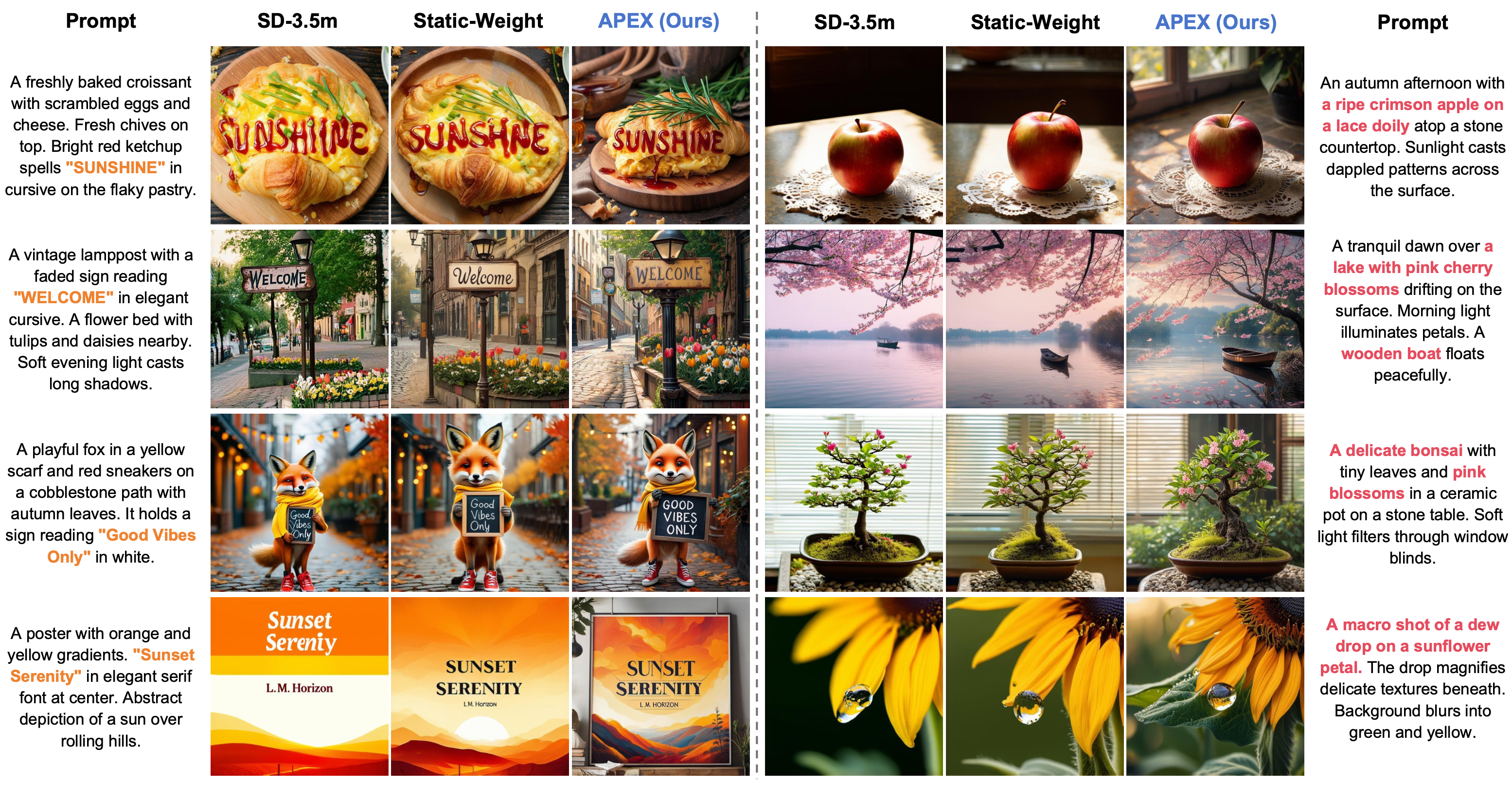
Instruction Alignment Accuracy. Although the Static-Weight method tends to prioritize local text features to achieve higher OCR scores in Table 1, APEX demonstrates superior comprehensive capability in coordinating text, semantics, and visuals. In tasks involving complex text rendering, APEX effectively addresses typical failure modes of baseline methods. Specifically, SD-3.5m and Static-Weight exhibit spelling errors or character deformations in Row 1 and Row 3, whereas APEX accurately renders the complete text while maintaining natural integration with the object’s texture. In Row 2, although Static-Weight generates clear fonts, the overly pristine texture of the sign contradicts the “vintage” stylistic constraint; in contrast, APEX precisely restores the weathered texture and ambient lighting while maintaining legibility. For the poster prompt in Row 4, which contains compositional ambiguity, APEX tends to construct a 3D scene with higher spatial complexity rather than a simple 2D layout, demonstrating its ability to explore diverse optimal solutions on the Pareto front.

Visual Detail Fidelity. In photorealistic rendering, APEX consistently outperforms the baselines in lighting modeling, color interaction, and physical logic, whereas Static-Weight shows limited improvement over SD-3.5m in these dimensions. A representative case is the cherry blossom lake (Row 6), where APEX achieves precise color isolation, preventing the background vegetation from being affected by “color-bleeding” from the pink blossoms, while capturing realistic reflections and atmospheric depth. Similar detail enhancements are evident in the delicate lace lighting (Row 5), the realistic bark textures and blind-filtered light (Row 7), and the physically-grounded dewdrop refraction and natural droplet distribution (Row 8). These observations suggest that APEX’s adaptive priority mechanism more effectively mines fine-grained, aesthetics-related reward signals.

The qualitative comparison corroborates the quantitative findings in Table 1: APEX effectively mitigates the “variance hijacking” phenomenon in multi-objective alignment. While maintaining competitiveness in key text metrics, it avoids semantic misalignment caused by overfitting a single objective, achieving a systemic balance between perceptual quality and instruction following.

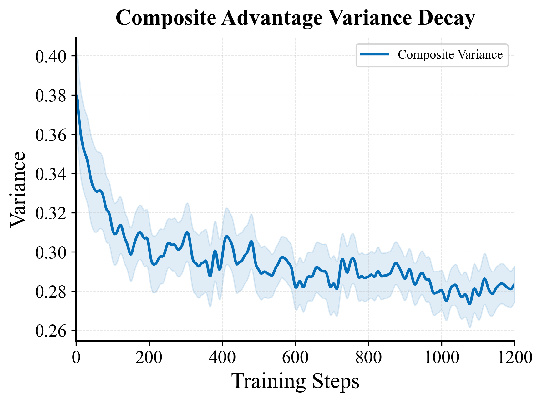
D.4 Composite Advantage Variance Dynamics

To verify the necessity of the second stage of DSAN normalization, we track the variance of the composite advantages after weighted aggregation but before the second normalization (Fig. 7). Experimental observations show a significant and continuous decay in advantage variance, dropping from $\sim 0.40$ initially to $\sim 0.28$ in the later stages. According to the principle of variance decomposition, while weight magnitudes remain relatively stable, the drop in total variance is attributed to the objective-wise covariance becoming negative. This statistically confirms that as training progresses, the model enters a “zero-sum game” region near the Pareto front, where gradient interference between objectives leads to signal cancellation. Without second-stage normalization, this natural variance decay would be equivalent to a passive reduction in the learning rate. APEX’s second-stage normalization provides an adaptive signal rescaling mechanism that forces the decayed composite advantages back to a standard distribution, compensating for signal loss caused by objective conflicts.

D.5 Stability Analysis of $\bm{\mathcal{P}^{3}}$ Factors

Figure 7: Composite Advantage Variance Decay. The weighted advantage variance decreases over training as DSAN normalizes conflicting gradients, reducing inter-objective interference.

Figure 8: Stability analysis of $\mathcal{P}^{3}$ factors. The Only-LP variant ($\alpha{=}0,\beta{=}0$) shows sudden spikes in KL divergence and clipping fraction, indicating unstable policy updates. APEX Full remains stable, confirming that CP and PN factors act as safety valves against gradient conflicts and objective saturation.

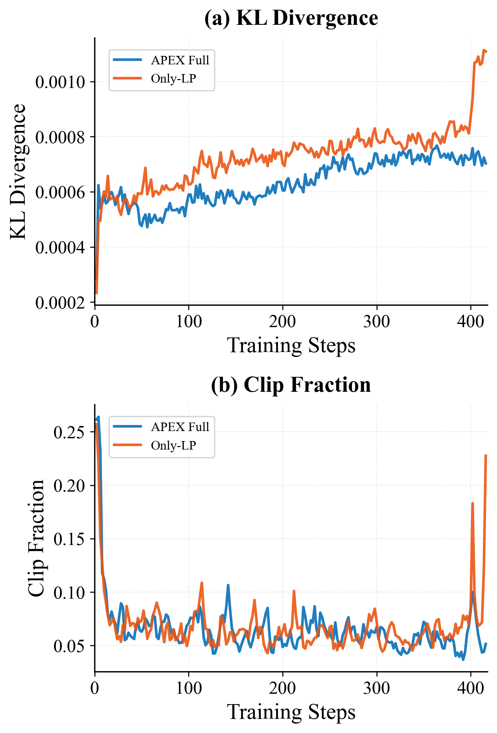
We reduce APEX to the Only-LP variant ($\alpha{=}0,\beta{=}0$), retaining only the learning potential factor. As shown in Fig. 8, the Only-LP variant performs similarly to APEX Full in the early stages, but as training deepens, its KL divergence and clipping fraction exhibit sudden, sharp spikes. This indicates that solely pursuing high gradient magnitude leads to overly aggressive policy updates. Without the constraints of Conflict Penalty (CP), the model forces updates when gradient directions are inconsistent, triggering parameter oscillations. Without Progress Need (PN) regulation, the model continues to apply high weights after certain objectives are saturated, causing the policy to deviate severely from the reference model. In contrast, APEX Full maintains a stable training trajectory throughout. This proves that the CP and PN factors serve as critical Safety Valves within the framework, ensuring convergence stability by dynamically suppressing excessive weight allocation during conflicts or objective saturation.

References

- Albergo et al. (2023) Michael S. Albergo, Nicholas M. Boffi, and Eric Vanden-Eijnden. 2023. Stochastic interpolants: A unifying framework for flows and diffusions. CoRR, abs/2303.08797.
- Anderson (1982) Brian D.O. Anderson. 1982. Reverse-time diffusion equation models. Stochastic Processes and their Applications, 12(3):313–326.
- Bie et al. (2025) Fengxiang Bie, Yibo Yang, Zhongzhu Zhou, Adam Ghanem, Minjia Zhang, Zhewei Yao, Xiaoxia Wu, Connor Holmes, Pareesa Ameneh Golnari, David A. Clifton, Yuxiong He, Dacheng Tao, and Shuaiwen Leon Song. 2025. Renaissance: A survey into AI text-to-image generation in the era of large model. IEEE Trans. Pattern Anal. Mach. Intell., 47(3):2212–2231.
- Black et al. (2024) Kevin Black, Michael Janner, Yilun Du, Ilya Kostrikov, and Sergey Levine. 2024. Training diffusion models with reinforcement learning. In The Twelfth International Conference on Learning Representations, ICLR 2024, Vienna, Austria, May 7-11, 2024. OpenReview.net.
- Clark et al. (2024) Kevin Clark, Paul Vicol, Kevin Swersky, and David J. Fleet. 2024. Directly fine-tuning diffusion models on differentiable rewards. In The Twelfth International Conference on Learning Representations, ICLR 2024, Vienna, Austria, May 7-11, 2024. OpenReview.net.
- Deb et al. (2002) K. Deb, A. Pratap, S. Agarwal, and T. Meyarivan. 2002. A fast and elitist multiobjective genetic algorithm: NSGA-II. IEEE Transactions on Evolutionary Computation, 6(2):182–197.
- Esser et al. (2024) Patrick Esser, Sumith Kulal, Andreas Blattmann, Rahim Entezari, Jonas Müller, Harry Saini, Yam Levi, Dominik Lorenz, Axel Sauer, Frederic Boesel, Dustin Podell, Tim Dockhorn, Zion English, and Robin Rombach. 2024. Scaling rectified flow transformers for high-resolution image synthesis. In Forty-first International Conference on Machine Learning.
- Fan et al. (2023) Ying Fan, Olivia Watkins, Yuqing Du, Hao Liu, Moonkyung Ryu, Craig Boutilier, Pieter Abbeel, Mohammad Ghavamzadeh, Kangwook Lee, and Kimin Lee. 2023. Dpok: Reinforcement learning for fine-tuning text-to-image diffusion models. In Advances in Neural Information Processing Systems, volume 36, pages 79858–79885. Curran Associates, Inc.
- Fonseca and Fleming (1996) Carlos M. Fonseca and Peter J. Fleming. 1996. On the performance assessment and comparison of stochastic multiobjective optimizers. In Parallel Problem Solving from Nature - PPSN IV, International Conference on Evolutionary Computation, Berlin, Germany, September 22-26, 1996, Proceedings, volume 1141 of Lecture Notes in Computer Science, pages 584–593. Springer.
- Fonseca et al. (2006) Carlos M. Fonseca, Luís Paquete, and Manuel López-Ibáñez. 2006. An improved dimension-sweep algorithm for the hypervolume indicator. In 2006 IEEE International Conference on Evolutionary Computation, CEC 2006, Vancouver, BC, Canada, July 16-21, 2006, pages 1157–1163. IEEE.
- Ho et al. (2020) Jonathan Ho, Ajay Jain, and Pieter Abbeel. 2020. Denoising diffusion probabilistic models. In Advances in Neural Information Processing Systems 33: Annual Conference on Neural Information Processing Systems 2020, NeurIPS 2020, December 6-12, 2020, virtual.
- Hu et al. (2022) Edward J. Hu, Yelong Shen, Phillip Wallis, Zeyuan Allen-Zhu, Yuanzhi Li, Shean Wang, Lu Wang, and Weizhu Chen. 2022. Lora: Low-rank adaptation of large language models. In The Tenth International Conference on Learning Representations, ICLR 2022, Virtual Event, April 25-29, 2022. OpenReview.net.
- Jiang et al. (2025) Dongzhi Jiang, Ziyu Guo, Renrui Zhang, Zhuofan Zong, Hao Li, Le Zhuo, Shilin Yan, Pheng-Ann Heng, and Hongsheng Li. 2025. T2I-R1: reinforcing image generation with collaborative semantic-level and token-level cot. CoRR, abs/2505.00703.
- Kirstain et al. (2023) Yuval Kirstain, Adam Polyak, Uriel Singer, Shahbuland Matiana, Joe Penna, and Omer Levy. 2023. Pick-a-pic: An open dataset of user preferences for text-to-image generation. In Advances in Neural Information Processing Systems 36: Annual Conference on Neural Information Processing Systems 2023, NeurIPS 2023, New Orleans, LA, USA, December 10 - 16, 2023.
- Kumar et al. (2023) Harshat Kumar, Alec Koppel, and Alejandro Ribeiro. 2023. On the sample complexity of actor-critic method for reinforcement learning with function approximation. Machine Learning, 112(7):2433–2467.
- Lee et al. (2024) Seung Hyun Lee, Yinxiao Li, Junjie Ke, Innfarn Yoo, Han Zhang, Jiahui Yu, Qifei Wang, Fei Deng, Glenn Entis, Junfeng He, Gang Li, Sangpil Kim, Irfan Essa, and Feng Yang. 2024. Parrot: Pareto-optimal multi-reward reinforcement learning framework for text-to-image generation. In Computer Vision - ECCV 2024 - 18th European Conference, Milan, Italy, September 29-October 4, 2024, Proceedings, Part XXXVIII, volume 15096 of Lecture Notes in Computer Science, pages 462–478. Springer.
- Lipman et al. (2023) Yaron Lipman, Ricky T. Q. Chen, Heli Ben-Hamu, Maximilian Nickel, and Matthew Le. 2023. Flow matching for generative modeling. In The Eleventh International Conference on Learning Representations, ICLR 2023, Kigali, Rwanda, May 1-5, 2023. OpenReview.net.
- Liu et al. (2025) Jie Liu, Gongye Liu, Jiajun Liang, Yangguang Li, Jiaheng Liu, Xintao Wang, Pengfei Wan, Di Zhang, and Wanli Ouyang. 2025. Flow-grpo: Training flow matching models via online RL. CoRR, abs/2505.05470.
- Lu et al. (2025) Yining Lu, Zilong Wang, Shiyang Li, Xin Liu, Changlong Yu, Qingyu Yin, Zhan Shi, Zixuan Zhang, and Meng Jiang. 2025. Learning to optimize multi-objective alignment through dynamic reward weighting. CoRR, abs/2509.11452.
- Lyu et al. (2025) Qiang Lyu, Zicong Chen, Chongxiao Wang, Haolin Shi, Shibo Gao, Ran Piao, Youwei Zeng, Jianlou Si, Fei Ding, Jing Li, Chun Pong Lau, and Weiqiang Wang. 2025. Multi-grpo: Multi-group advantage estimation for text-to-image generation with tree-based trajectories and multiple rewards. Preprint, arXiv:2512.00743.
- Marler and Arora (2004) R Timothy Marler and Jasbir S Arora. 2004. Survey of multi-objective optimization methods for engineering. Structural and multidisciplinary optimization, 26(6):369–395.
- Øksendal (2003) Bernt Øksendal. 2003. Stochastic differential equations. In Stochastic differential equations: an introduction with applications, pages 38–50. Springer.
- Rombach et al. (2022) Robin Rombach, Andreas Blattmann, Dominik Lorenz, Patrick Esser, and Björn Ommer. 2022. High-resolution image synthesis with latent diffusion models. In IEEE/CVF Conference on Computer Vision and Pattern Recognition, CVPR 2022, New Orleans, LA, USA, June 18-24, 2022, pages 10674–10685. IEEE.
- Saharia et al. (2022) Chitwan Saharia, William Chan, Saurabh Saxena, Lala Li, Jay Whang, Emily L Denton, Kamyar Ghasemipour, Raphael Gontijo Lopes, Burcu Karagol Ayan, Tim Salimans, Jonathan Ho, David J Fleet, and Mohammad Norouzi. 2022. Photorealistic text-to-image diffusion models with deep language understanding. In Advances in Neural Information Processing Systems, volume 35, pages 36479–36494. Curran Associates, Inc.
- Schuhmann et al. (2022) Christoph Schuhmann, Romain Beaumont, Richard Vencu, Cade Gordon, Ross Wightman, Mehdi Cherti, Theo Coombes, Aarush Katta, Clayton Mullis, Mitchell Wortsman, Patrick Schramowski, Srivatsa Kundurthy, Katherine Crowson, Ludwig Schmidt, Robert Kaczmarczyk, and Jenia Jitsev. 2022. Laion-5b: An open large-scale dataset for training next generation image-text models. In Advances in Neural Information Processing Systems, volume 35, pages 25278–25294. Curran Associates, Inc.
- Shao et al. (2024) Zhihong Shao, Peiyi Wang, Qihao Zhu, Runxin Xu, Junxiao Song, Xiao Bi, Haowei Zhang, Mingchuan Zhang, Y. K. Li, Y. Wu, and Daya Guo. 2024. Deepseekmath: Pushing the limits of mathematical reasoning in open language models. Preprint, arXiv:2402.03300.
- Wang et al. (2017) Yue Wang, Wei Chen, Yuting Liu, Zhi-Ming Ma, and Tie-Yan Liu. 2017. Finite sample analysis of the GTD policy evaluation algorithms in Markov setting. In Advances in Neural Information Processing Systems, volume 30, pages 5504–5513. Curran Associates, Inc.
- Xu et al. (2023) Jiazheng Xu, Xiao Liu, Yuchen Wu, Yuxuan Tong, Qinkai Li, Ming Ding, Jie Tang, and Yuxiao Dong. 2023. Imagereward: Learning and evaluating human preferences for text-to-image generation. In Advances in Neural Information Processing Systems, volume 36, pages 15903–15935. Curran Associates, Inc.
- You et al. (2025) Zhiyuan You, Xin Cai, Jinjin Gu, Tianfan Xue, and Chao Dong. 2025. Teaching large language models to regress accurate image quality scores using score distribution. In IEEE/CVF Conference on Computer Vision and Pattern Recognition, CVPR 2025, Nashville, TN, USA, June 11-15, 2025, pages 14483–14494. Computer Vision Foundation / IEEE.
- Zhang et al. (2024) Sixian Zhang, Bohan Wang, Junqiang Wu, Yan Li, Tingting Gao, Di Zhang, and Zhongyuan Wang. 2024. Learning multi-dimensional human preference for text-to-image generation. In 2024 IEEE/CVF Conference on Computer Vision and Pattern Recognition (CVPR), pages 8018–8027.
- Ziegler et al. (2020) Daniel M. Ziegler, Nisan Stiennon, Jeffrey Wu, Tom B. Brown, Alec Radford, Dario Amodei, Paul Christiano, and Geoffrey Irving. 2020. Fine-tuning language models from human preferences. Preprint, arXiv:1909.08593.
- Zitzler and Thiele (1999) Eckart Zitzler and Lothar Thiele. 1999. Multiobjective evolutionary algorithms: A comparative case study and the strength pareto approach. IEEE Trans. Evol. Comput., 3(4):257–271.