A finite element method preserving the eigenvalue range of symmetric tensor fieldsThanks:  Department of Mathematics and Statistics, University of Strathclyde, 26 Richmond Street, Glasgow G1 1XK, UK, abdolreza.amiri@strath.ac.uk. Thanks:  Department of Mathematics and Statistics, University of Strathclyde, 26 Richmond Street, Glasgow G1 1XK, UK, gabriel.barrenechea@strath.ac.uk. Thanks:  Department of Mathematical Sciences, University of Bath, Bath BA2 7AY, UK tmp38@bath.ac.uk.

Abstract.

This paper presents a finite element method that preserves (at the degrees of freedom) the eigenvalue range of the solution of tensor-valued time-dependent convection–diffusion equations. Starting from a high-order spatial baseline discretisation (in this case, the CIP stabilised finite element method), our approach formulates the fully discrete problem as a variational inequality posed on a closed convex set of tensor-valued functions that respect the same eigenvalue bounds at their degrees of freedom. The numerical realisation of the scheme relies on the definition of a projection that, at each node, performs the diagonalisation of the tensor and then truncates the eigenvalues to lie within the prescribed bounds. The temporal discretisation is carried out using the implicit Euler method, and unconditional stability and optimal-order error estimates are proven for this choice. Numerical experiments confirm the theoretical findings and illustrate the method’s ability to maintain eigenvalue constraints while accurately approximating solutions in the convection-dominated regime.

Keywords : Tensor-valued PDEs, eigenvalue range, continuous interior penalty, finite element method, convection-diffusion equations, error estimates

1. Introduction

Motivation.

Tensor-valued partial differential equations (PDEs) arise in many settings where the primary unknown is more naturally represented by a symmetric tensor field than by a scalar or a vector. Examples include elasticity [Hug12], non-Newtonian fluid mechanics [OP02], diffusion tensor imaging [BML94] and liquid crystal modelling [dGP93]. In these applications, the tensor’s eigenvalues typically have a direct physical meaning and are required to satisfy pointwise bounds. In diffusion tensor imaging, positive definiteness is essential to represent meaningful diffusion processes [AFPA06]. In computational solid mechanics, constraints on the eigenvalues of stress and strain are tied to stability and admissibility of material responses [SH92]. In viscoelastic and other non-Newtonian models the conformation or extra-stress tensor is positive definite [AP25] and, in some cases such as FENE-P, additional constraints such as a bounded trace are imposed, see [OP02].

Standard discretisations for convection-diffusion-type PDEs do not typically enforce eigenvalue constraints. In particular, continuous Galerkin finite element methods [EG21, BS08], finite volume schemes [LeV02] and spectral methods [CHQZ07] may generate approximations whose eigenvalues violate prescribed bounds, especially in convection-dominated regimes or near sharp fronts. Such violations can lead to non-physical states and may trigger numerical instabilities or loss of robustness, even when the underlying continuous model preserves admissibility.

Contributions of this work.

We develop a finite element method for time-dependent convection–diffusion equations with symmetric tensor unknowns that preserves a prescribed eigenvalue range $[\epsilon,\kappa]$, with $\epsilon<\kappa$, at the degrees of freedom. The method extends recent nodally bound-preserving finite element ideas from scalar to tensor-valued problems by combining a baseline stabilised discretisation with a convex admissible set of tensor-valued finite element functions whose nodal values satisfy the eigenvalue bounds. The fully discrete scheme is formulated and analysed as a variational inequality over this admissible set. For its numerical realisation we employ an iterative solver based on a nodal projection defined by local spectral decomposition followed by eigenvalue truncation. For time discretisation we use implicit Euler, and for space discretisation we use continuous interior penalty (CIP), which provides stabilisation in the convection-dominated regime [BH04, BF09]. We prove unconditional stability and derive a priori error estimates for the fully discrete method. Numerical experiments illustrate that the approach prevents eigenvalue over- and undershoots observed in the baseline scheme, while retaining good accuracy for both smooth and non-smooth data.

Relation to the literature.

The design of bound-preserving discretisations, often discussed in the context of the discrete maximum principle (DMP), has a long history. Early analytical results for maximum principles in finite element methods date back to [CR73]. In general, however, standard Galerkin schemes on arbitrary meshes do not satisfy the DMP for convection–diffusion problems, leading to spurious oscillations and unphysical overshoots. This difficulty motivated a range of remedies. One classical approach is to add artificial diffusion or to employ upwinding to stabilise the scheme, including early artificial-viscosity ideas in the finite element setting [Kik77] and nonlinear Petrov–Galerkin upwind constructions designed to enforce a maximum principle in convection-dominated regimes [MH85]. For piecewise linear elements, the DMP can be guaranteed under restrictive geometric or algebraic conditions, for example acute simplicial meshes or an $M$-matrix structure of the stiffness operator [BKK08]. As a consequence, many modern bound-preserving methods are necessarily nonlinear and rely on added stabilisation, limiters or algebraic corrections to eliminate new extrema, consistent with the classical limitations on linear high-order monotone schemes. Representative finite element approaches include CIP-type stabilisation augmented by nonlinear diffusion to recover a DMP [BE05] and edge-based nonlinear diffusion mechanisms closely connected to algebraic flux-correction techniques [BBK17]. In parallel, the flux-corrected transport (FCT) and algebraic flux-correction (AFC) paradigms modify the algebraic form of the discrete operator by limiting antidiffusive fluxes so as to enforce bounds while retaining accuracy [Kuz07]. Variants and extensions of these ideas, including multiscale and constraint-enforcement perspectives, are discussed in [EHS09]. A broad and up-to-date account of monotonicity-preserving and DMP-related finite element methodology can be found in the recent monograph [BJK25] and the references therein.

Beyond maximum-principle preservation for scalar problems, a closely related body of work concerns invariant-domain and structure-preserving discretisations for systems, where admissibility is expressed through convex invariant sets, entropy inequalities or energy dissipation. In the discontinuous Galerkin setting, such questions are often addressed through a combination of stabilisation and limiting, with analysis frequently organised around entropy or relative-entropy frameworks, see for instance [GMP15, GP16a]. Although these developments do not directly target tensor eigenvalue constraints, they provide a useful methodological backdrop, they highlight how nonlinear admissibility requirements typically enter either through limiters applied to a baseline high-order method or through constrained variational principles.

For tensor-valued problems, the literature on bound-preserving schemes is far more limited. To the best of our knowledge, the main existing contributions that explicitly preserve eigenvalue ranges for transported symmetric tensors are [Loh17, Loh19]. These works extend FCT and AFC ideas to matrix-valued unknowns, with limiting strategies designed to prevent the loss of key admissibility properties such as positive definiteness during transport. Beyond these contributions, eigenvalue control for tensor quantities is more commonly addressed indirectly, for example through problem-specific reconstructions or limiters in hyperbolic and remap-type algorithms, rather than through a systematic finite element framework.

A different line of work enforces admissibility through nonlinear transformations rather than direct limiting. In the context of symmetric positive-definite (SPD) tensor fields, geometric constructions based on the matrix logarithm provide parametrisations in which SPD is preserved by construction [AFPA06, Moa05]. In non-Newtonian fluid mechanics, the log-conformation representation is a prominent example of this philosophy [FK04]. While such transformations can be effective, they introduce additional nonlinear structure and can complicate both analysis and implementation when combined with standard stabilisation and time-stepping strategies, particularly in convection-dominated regimes.

The present work is most closely related to recent developments on nodally bound-preserving finite element methods for scalar problems. The framework in [BGPV24] constrains nodal degrees of freedom to lie in an admissible range by projection onto a convex nodal set and, in certain settings, admits an interpretation as a variational inequality. This viewpoint aligns with the broader theory of constrained energy minimisation and variational inequalities that underpins many finite element treatments of inequality constraints [KS00, KS24b, KS24a]. Time-dependent extensions to reaction–convection–diffusion and related parabolic problems have been developed in [ABP24, ABP25], with the essential mechanism remaining a baseline discretisation coupled to a nonlinear admissibility enforcement at each time level.

These nodal approaches sit alongside a closely related line of work on invariant-domain and convex-limiting strategies for continuous finite element discretisations of hyperbolic systems, where admissibility is formulated in terms of convex invariant sets and recovered a posteriori by limiting a high-order update towards a low-order invariant-domain update [GNPY14, GP16b, GPT19]. In the discontinuous Galerkin setting, a complementary and extensive literature establishes positivity-preserving and invariant-domain ideas via cell-average constraints and limiters compatible with SSP time integrators [ZS10, ZS11]. Although these strands differ in their admissibility variables (nodal values versus cell averages or local invariant sets) and in the underlying discretisation class (continuous versus discontinuous Galerkin), they share the same organising principle, a baseline scheme is augmented by a nonlinear correction that enforces an admissible set without destroying accuracy away from constrained regions.

Further developments of nodal admissibility ideas beyond the original scalar convection–diffusion setting include extensions to drift–diffusion-type models and to hyperbolic convection–reaction problems, illustrating the flexibility of the projection/constraint paradigm across different PDE structures [BPT25, AHP25]. Here, this line of ideas is extended from scalar to tensor-valued convection–diffusion equations by formulating a variational inequality directly on an admissible set defined through nodal eigenvalue constraints, using a CIP baseline discretisation. This provides a route to enforce physically motivated tensor constraints while retaining a standard finite element setting and allowing convection-dominated stabilisation.

The paper is organised as follows. In Section 2 we introduce notation and preliminary results. In Section 3 we present the model problem, the finite element spaces, the key inequalities used in the analysis and the admissible convex set. Section 4 introduces the fully discrete variational inequality formulation. Stability and convergence are proved in Section 5. Numerical experiments are presented in Section 6. Concluding remarks and possible extensions are given in Section 7.

2. Notation and Preliminaries

Let us consider the space of symmetric tensors of dimension $d\times d$, $1\leq d\leq 3$. We denote this space by $\mathbb{S}_{d}\subset\mathbb{R}^{d\times d}$, while $\mathbb{S}_{d}^{+}$ stands for the subset of positive semidefinite tensors. Table 1 summarises the symbols frequently used in this work.

Table 1. Summary of symbols frequently used in this work.

Symbol	Description
$d$	Dimension of the tensor
$m$	Dimension of the space (i.e., $\Omega\subset\mathbb{R}^{m}$)
$k,\ell$	Indices corresponding to tensor components, i.e. $1\leq k,\ell\leq d$
$\mathbb{S}_{d}$	Space of symmetric tensors in $\mathbb{R}^{d\times d}$
$\mathbf{0}$	Zero tensor
$\mathbf{I}$	Identity tensor
$v_{k\ell}$	Tensor entry of $\mathbf{V}\in\mathbb{S}_{d}$
$\tilde{\mathbf{V}}=\mathrm{diag}(\lambda_{1},\lambda_{2},\ldots,\lambda_{d})$	Diagonal tensor with eigenvalues of $\mathbf{V}\in\mathbb{S}_{d}$ on its diagonal
$\mathbf{x}$	Vector in $\mathbb{R}^{m}$
$\mathbf{V}=\mathbf{Q}_{\mathbf{V}}\tilde{\mathbf{V}}\mathbf{Q}^{T}_{\mathbf{V}}$	Spectral decomposition of $\mathbf{V}\in\mathbb{S}_{d}$

Additionally, we adopt the notation that lowercase bold letters such as $\mathbf{v}\in\mathbb{R}^{d}$ denote $d$-dimensional vectors, while uppercase bold letters, such as $\mathbf{U}$ and $\mathbf{V}$, are reserved for tensor quantities.

Since all the tensors in this manuscript are symmetric, they are diagonalisable. So, they admit the decomposition

(1) $$\mathbf{V}=\mathbf{Q}_{\mathbf{V}}\tilde{\mathbf{V}}\mathbf{Q}^{T}_{\mathbf{V}}\quad\textrm{where}\quad\tilde{\mathbf{V}}:={\rm diag}(\lambda_{1},\lambda_{2},\ldots,\lambda_{d})\quad,\quad\mathbf{Q}_{\mathbf{V}}^{T}\mathbf{Q}_{\mathbf{V}}=\mathbf{I}.$$

Above, as standard, $\tilde{\mathbf{V}}$ denotes the diagonal tensor of sorted eigenvalues $\lambda_{k}(\mathbf{V})$ of $\mathbf{V}$, and $\mathbf{Q}_{\mathbf{V}}$ is the tensor of corresponding eigenvectors of $\mathbf{V}$. Whenever it is clear from the context, we omit $\mathbf{V}$ from $\lambda_{k}(\mathbf{V})$ for simplicity and we use $\lambda_{k}$.

Since this work will focus on preserving the eigenvalue range of symmetric tensors, for $\epsilon\geq 0$ and $\kappa>\epsilon$, we define the following convex subset of $\mathbb{S}_{d}$

(2) $$\mathbb{S}_{d}^{\epsilon,\kappa}:=\{\mathbf{V}\in\mathbb{S}_{d}:\epsilon\leq\lambda_{1}\leq\lambda_{2}\leq\ldots\leq\lambda_{d}\leq\kappa\}.$$

(This is a closed convex set in $\mathbb{S}_{d}$.) Here $\lambda_{k}$, $k=1,\ldots,d$ are sorted eigenvalues of $\mathbf{V}$. Using this convex subset, we decompose every element $\mathbf{V}\in\mathbb{S}_{d}$ as the sum $\mathbf{V}=\mathbf{V}^{+}+\mathbf{V}^{-}$, where $\mathbf{V}^{+}$ and $\mathbf{V}^{-}$ are given by

(3) $$\mathbf{V}^{+}=\mathbf{Q}_{\mathbf{V}}\tilde{\mathbf{V}}^{+}\mathbf{Q}^{T}_{\mathbf{V}},$$

where the $k$th diagonal entry of $\tilde{\mathbf{V}}^{+}$ is defined as

(4) $$(\lambda_{k}(\mathbf{V}))^{+}=\max\Big\{\epsilon,\min\{\lambda_{k}(\mathbf{V}),\kappa\}\Big\}$$

and

(5) $$\mathbf{V}^{-}=\mathbf{V}-\mathbf{V}^{+}.$$

In this paper we will make use of the Frobenius norm $\|\cdot\|_{F}$. Therefore, we summarise some of its most important properties. According to the invariance of the trace $\text{tr}(\cdot)$ under cyclic permutations,

$$\text{tr}(\mathbf{V}\mathbf{W})=\text{tr}(\mathbf{W}\mathbf{V}),\quad\text{for all }\mathbf{V},\mathbf{W}\in\mathbb{R}^{d\times d},$$

and the definition of the Frobenius inner product $(\cdot,\cdot)_{F}$,

(6) $$(\mathbf{V},\mathbf{W})_{F}:=\mathbf{V}:\mathbf{W}=\sum_{k,\ell=1}^{d}v_{k\ell}w_{k\ell}=\text{tr}(\mathbf{V}^{\top}\mathbf{W})=\text{tr}(\mathbf{W}^{\top}\mathbf{V}),$$

the Frobenius norm $\|\cdot\|_{F}$ satisfies the identity

(7) $$\|\mathbf{V}\|_{F}^{2}:=(\mathbf{V},\mathbf{V})_{F}=\text{tr}(\mathbf{V}^{\top}\mathbf{V})=\text{tr}((\mathbf{Q}^{\top}\mathbf{V}\mathbf{Q})^{\top}\mathbf{Q}^{\top}\mathbf{V}\mathbf{Q})=\sum_{k=1}^{d}\lambda_{k}^{2},\quad\text{for all }\mathbf{V}\in\mathbb{S}_{d}.$$

We will adopt standard notations for Sobolev spaces in line with, e.g., [EG21]. For $D\subseteq\mathbb{R}^{m}$, $m=1,2,3$, we denote by $\|\cdot\|_{0,p,D}$ the $L^{p}(D)$-norm; when $p=2$ the subscript $p$ will be omitted and we only write $\|\cdot\|_{0,D}$. In addition, for $s\geq 0$, $p\in[1,\infty]$, we denote by $\|\cdot\|_{s,p,D}$ ($|\cdot|_{s,p,D}$) the norm (seminorm) in $W^{s,p}(D)$; when $p=2$, we define $H^{s}(D)=W^{s,2}(D)$, and again omit the subscript $p$ and only write $\|\cdot\|_{s,D}$ ($|\cdot|_{s,D}$). The following space will also be used repeatedly within the text

(8) $$H^{1}_{0}(D)=\left\{v\in H^{1}(D):v=0\;{\rm on}\;\partial D\right\},$$

and the space $H^{-1}(D)$ which is the dual of $H^{1}_{0}(D)$.

For $1\leq p\leq+\infty$, $L^{p}((0,T);W^{s,p}(D))$ is the space defined by

$$L^{p}((0,T);W^{s,p}(D))=\left\{u(t,\cdot)\in W^{s,p}(D)~~\text{for almost all $t\in[0,T]$}:t\mapsto\|u(t,\cdot)\|_{s,p,D}\in L^{p}(0,T)\right\},$$

which is a Banach space for the norm

$$\begin{split}\|u\|_{L^{p}((0,T);W^{s,p}(D))}=\left\{\begin{array}[]{ll}\left(\int_{0}^{T}\|u\|_{s,p,D}^{p}dt\right)^{\frac{1}{p}}\hskip 65.44142pt{\rm if}\hskip 5.69046pt1\leq p<\infty,\\ \\ {\rm ess}\hskip 1.42271pt\sup_{t\in(0,T)}\|u\|_{s,p,D}\hskip 54.06006pt{\rm if}\hskip 8.5359ptp=\infty.\end{array}\right.\end{split}$$

The extension of the Sobolev norms to the vector and tensor-valued cases is straightforward. In fact, the inner product in $L^{2}(D)^{d\times d}$ is defined as

(9) $$(\mathbf{U},\mathbf{V})_{D}=\sum_{k,\ell=1}^{d}\int_{D}u_{k\ell}v_{k\ell}{\rm d}\boldsymbol{x}=\int_{D}\mathbf{U}:\mathbf{V}{\rm d}\boldsymbol{x},$$

which induces the norm $\|\mathbf{U}\|_{0,D}=(\mathbf{U},\mathbf{U})_{D}^{\frac{1}{2}}$. Using similar definitions for the derivatives we can extend the Sobolev norms to vector and tensor-valued quantities. Finally, we will use the following Sobolev space

(10) $$(H^{1}_{0}(D))^{d\times d,\textrm{sym}}=\left\{\mathbf{V}\in(H^{1}_{0}(D))^{d\times d}:\mathbf{V}\in\mathbb{S}_{d}\;\textrm{a.e. in}\;D\right\}.$$

3. The model problem

Let $\Omega$ be an open bounded Lipschitz domain in $\mathbb{R}^{m}$ ($m=2,3$) with polyhedral boundary $\partial\Omega$, and $T>0$. For a given $\mathbf{F}\in(L^{2}((0,T);L^{2}(\Omega)))^{d\times d}$, we consider the following convection-diffusion problem:

(11) $$\begin{split}\left\{\begin{aligned} \partial_{t}\mathbf{U}-{\rm div}\big(\mathcal{D}\nabla\mathbf{U}\big)+{\boldsymbol{\beta}}\cdot\nabla\mathbf{U}+\mu\mathbf{U}&=\mathbf{F}&&\text{in }(0,T]\times\Omega,\\ \mathbf{U}(\boldsymbol{x},t)&=0&&\text{on }(0,T]\times\partial\Omega,\\ \mathbf{U}(\cdot,0)&=\mathbf{U}^{0}&&\text{in }\Omega,\end{aligned}\right.\end{split}$$

where $\mathcal{D}=(d_{ij})_{i,j=1}^{m}\in[L^{\infty}(\Omega)]^{m\times m}$ is symmetric and uniformly strictly positive definite a.e. in $\Omega$, ${\boldsymbol{\beta}}=(\beta_{i})_{i=1}^{m}\in L^{\infty}((0,T);W^{1,\infty}(\Omega))^{m}$, and $\mu\in\mathbb{R}^{+}_{0}$, respectively, are the diffusion coefficient, the convective field, and the reaction coefficient. We will assume that ${\rm div}{\boldsymbol{\beta}}=0$ in $\Omega\times[0,T]$.

Remark 3.1 (Componentwise interpretation of the transport terms).

In equation (11), the diffusion term ${\rm div}(\mathcal{D}\nabla\mathbf{U})$ involves the action of the tensor $\mathcal{D}\in\mathbb{R}^{m\times m}$ on $\nabla\mathbf{U}\in\mathbb{R}^{d\times d\times m}$ which is a multilinear operator (see e.g. [AA21]). The product $\mathcal{D}\nabla\mathbf{U}$ is understood as the following tensor product

(12) $$\mathcal{D}\nabla\mathbf{U}=\begin{pmatrix}\mathcal{D}\nabla U_{11}&\cdots&\mathcal{D}\nabla U_{1d}\\ \vdots&\ddots&\vdots\\ \mathcal{D}\nabla U_{d1}&\cdots&\mathcal{D}\nabla U_{dd}\end{pmatrix},$$

so that the $(k,\ell)$-th component of the diffusion term is ${\rm div}\big(\mathcal{D}\nabla U_{k\ell}\big)$. The convection term ${\boldsymbol{\beta}}\cdot\nabla\mathbf{U}$ is defined similarly, i.e. $({\boldsymbol{\beta}}\cdot\nabla\mathbf{U})_{k\ell}={\boldsymbol{\beta}}\cdot\nabla U_{k\ell}$.

The standard weak formulation of (11) reads as follows: Find $\mathbf{U}\in L^{\infty}((0,T);(H^{1}_{0}(\Omega))^{d\times d,\textrm{sym}})\cap\left(H^{1}((0,T);H^{-1}(\Omega))\right)^{d\times d,\textrm{sym}}$ such that, for almost all $t\in(0,T)$ the following holds

(13) $$\begin{split}\left\{\begin{array}[]{ll}(\partial_{t}\mathbf{U},\mathbf{V})_{\Omega}+a(\mathbf{U},\mathbf{V})=(\mathbf{F},\mathbf{V})_{\Omega}\hskip 28.45274pt\forall\mathbf{V}\in\left(H^{1}_{0}(\Omega)\right)^{d\times d,\textrm{sym}},\\ \hskip 45.52458pt\mathbf{U}(\cdot,0)=\mathbf{U}^{0}.\end{array}\right.\end{split}$$

Here, the bilinear form $a(\cdot,\cdot)$ is defined by

(14) $$a(\mathbf{W},\mathbf{V}):=\left(\mathcal{D}\nabla\mathbf{W},\nabla\mathbf{V}\right)_{\Omega}+({\boldsymbol{\beta}}\cdot\nabla\mathbf{W},\mathbf{V})_{\Omega}+\mu(\mathbf{W},\mathbf{V})_{\Omega}.$$

In the above definition we have slightly abused the notation, as the convective term ${\boldsymbol{\beta}}$ might depend on $t$, but unless the context requires it, we will always denote this bilinear form by $a(\cdot,\cdot)$. Since we have supposed that ${\boldsymbol{\beta}}$ is solenoidal, then the bilinear form $a(\cdot,\cdot)$ is elliptic, in the sense that for $\mathbf{V}\in(H^{1}_{0}(\Omega))^{d\times d}$ it holds that $({\boldsymbol{\beta}}\cdot\nabla\mathbf{V},\mathbf{V})_{\Omega}=0$ and hence $a(\mathbf{V},\mathbf{V})=(\mathcal{D}\nabla\mathbf{V},\nabla\mathbf{V})_{\Omega}+\mu(\mathbf{V},\mathbf{V})_{\Omega}$. More precisely, for each $t\in(0,T)$ the bilinear form $a(\cdot,\cdot)$ induces the following “energy” norm in $\left(H^{1}_{0}(\Omega)\right)^{d\times d}$

$$\|\mathbf{V}\|_{a}=\left(a(\mathbf{V},\mathbf{V})\right)^{\frac{1}{2}},\qquad t\in[0,T].$$

It is a well-known fact that the problem (13) has a unique solution $\mathbf{U}$, as a consequence of Lions’ Theorem (see, e.g., [LM12, Theorem 4.1]). Building on what was mentioned in the introduction, we will make the following assumption on $\mathbf{U}$.

Assumption (A1): We will suppose that the eigenvalues of the weak solution of (13) satisfy

(15) $$\epsilon\leq\lambda_{k}(\mathbf{U}(\boldsymbol{x},t))\leq\kappa,\hskip 14.22636ptk=1,\cdots,d,\hskip 14.22636pt\text{ for almost all}\ \ (\boldsymbol{x},t)\in\Omega\times(0,T),$$

where $\epsilon$ and $\kappa$ are known non-negative constants.

3.1. Space discretisation

Since in problem (13) the space and time variables play different roles, we first approximate the solution in (13) only in space, reducing it to a system of coupled ordinary differential equations where time is the only independent variable.

To discretise (13) with respect to space in tensor form, we consider a finite-dimensional subspace of $(H^{1}(\Omega))^{d\times d}$. Let ${\mathcal{P}}$ be a conforming and shape-regular partition of $\Omega$ into simplices (or affine quadrilateral/hexahedra). We denote by $\boldsymbol{x}_{1},\ldots,\boldsymbol{x}_{M}$ the interior nodes of ${\mathcal{P}}$. Over ${\mathcal{P}}$, and for $k\geq 1$, we define the tensor finite element space as

(16) $$\mathbb{V}_{\mathcal{P}}:=\{\mathbf{V}_{h}\in(C^{0}(\overline{\Omega}))^{d\times d}:\mathbf{V}_{h}|_{K}\in(\mathfrak{R}(K))^{d\times d},\ \forall K\in{\mathcal{P}}\}\cap(H_{0}^{1}(\Omega))^{d\times d,\textrm{sym}},$$

where

(17) $$\mathfrak{R}(K)=\begin{cases}\mathbb{P}_{k}(K),&\text{if }K\text{ is a simplex},\\ \mathbb{Q}_{k}(K),&\text{if }K\text{ is an affine quadrilateral/hexahedral},\end{cases}$$

with $\mathbb{P}_{k}(K)$ denoting the polynomials of total degree $k$ on $K$ and $\mathbb{Q}_{k}(K)$ denoting the mapped space of polynomials of degree at most $k$ in each variable.

Remark 3.2 (Tensor-valued basis construction).

There are several ways in which the basis functions for this space can be built. We now give some more details on this process. Let $V_{\mathcal{P}}$ denote the scalar finite element space defined as

(18) $$V_{\mathcal{P}}:=\{v_{h}\in C^{0}(\overline{\Omega}):v_{h}|_{K}\in\mathfrak{R}(K),\forall K\in{\mathcal{P}}\}\cap H^{1}_{0}(\Omega),$$

with basis functions $\{\phi_{i}\}_{i=1}^{M}$. Therefore, based on the definition of the finite element space $\mathbb{V}_{{\mathcal{P}}}$, any function $\mathbf{V}_{h}\in\mathbb{V}_{{\mathcal{P}}}$ can be represented by the following expansion

(19) $$\mathbf{V}_{h}=\sum_{i=1}^{M}\sum_{1\leq j\leq\ell\leq d}v_{j\ell}^{i}\Phi^{j\ell}_{i},$$

where $\Phi^{j\ell}_{i}$ are the tensor-valued basis functions given by

(20) $$\Phi^{j\ell}_{i}=\begin{cases}\phi_{i}\mathbf{e}_{j}\otimes\mathbf{e}_{j},&\text{if }j=\ell,\\ \phi_{i}(\mathbf{e}_{j}\otimes\mathbf{e}_{\ell}+\mathbf{e}_{\ell}\otimes\mathbf{e}_{j}),&\text{if }j<\ell.\end{cases}$$

Here, $\mathbf{e}_{j}$ is the $j$-th canonical basis vector in $\mathbb{R}^{d}$, $v_{j\ell}^{i}$ are the coefficients of the expansion, and $\otimes$ denotes the tensor product. The tensor-valued basis functions $\Phi^{j\ell}_{i}$ are constructed to preserve the symmetry of the elements of $\mathbb{V}_{{\mathcal{P}}}$. In particular, for $j<\ell$ the symmetric combination in (20) ensures that $\Phi^{j\ell}_{i}$ has equal $(j,\ell)$ and $(\ell,j)$ components. Note that since the tensor space $\mathbb{V}_{{\mathcal{P}}}$ consists of symmetric tensors, its dimension is $M\frac{d(d+1)}{2}$.

The natural extension of the Lagrange interpolation operator (see [EG21, Chapter 11] for its definition) to the tensor-valued context is the following mapping

$$\mathbf{I}_{h}:\big(\mathcal{C}^{0}(\overline{\Omega})\big)^{d\times d}\cap\big(H^{1}_{0}(\Omega)\big)^{d\times d,\textrm{sym}} \longrightarrow\mathbb{V}_{\mathcal{P}},$$

(21) $$\mathbf{V} \longmapsto\mathbf{I}_{h}\mathbf{V}:=\sum_{i=1}^{M}\sum_{k,\ell=1}^{d}v_{k\ell}(\boldsymbol{x}_{i})\Phi^{k\ell}_{i}.$$

(Here the interpolation is defined componentwise by evaluating $\mathbf{V}$ at the nodal points $\boldsymbol{x}_{i}$ and expanding in the tensor-valued basis from (20).) It satisfies the following approximation property (see [EG21, Proposition 1.12]): Let $1\leq\ell\leq k$. Then there exists $C>0$, independent of $h$, such that for all $\mathbf{V}\in(H^{\ell+1}(\Omega))^{d\times d}\cap(H^{1}_{0}(\Omega))^{d\times d}$,

(22) $$\|\mathbf{V}-\mathbf{I}_{h}\mathbf{V}\|_{0,K}+h_{K}|\mathbf{V}-\mathbf{I}_{h}\mathbf{V}|_{1,K}\leq Ch^{\ell+1}_{K}|\mathbf{V}|_{\ell+1,K}.$$

In addition, we recall some standard estimates for finite element functions, presented here in the tensor-valued form. First, we recall the following inverse inequality (see [EG21, Lemma 12.1]): for all $s,\ell\in\mathbb{N}_{0}$, $0\leq s\leq\ell$ and all $p,q\in[1,\infty]$, there exists a constant $C>0$, independent of $h$, such that for all $\mathbf{V}_{h}\in\mathbb{V}_{\mathcal{P}}$

(23) $$|\mathbf{V}_{h}|_{\ell,p,K}\leq Ch_{K}^{s-\ell+m\left(\frac{1}{p}-\frac{1}{q}\right)}|\mathbf{V}_{h}|_{s,q,K}.$$

(The exponent involves the spatial dimension $m$ of $\Omega\subset\mathbb{R}^{m}$, rather than the tensor dimension $d$.) In addition, we recall the following discrete trace inequality (see [EG21, Lemma 2.15]): there exists $C>0$ independent of $h$ such that, for every $\mathbf{V}\in(H^{1}(K))^{d\times d}$,

(24) $$\|\mathbf{V}\|^{2}_{0,\partial K}\leq C\left(h_{K}^{-1}\|\mathbf{V}\|^{2}_{0,K}+h_{K}|\mathbf{V}|^{2}_{1,K}\right).$$

3.2. The baseline discretisation

As discussed in the introduction, the method is built over a baseline discretisation. For convection-dominated (or transport) problems, it is a well-established fact that the plain Galerkin method should not be used. So, in this work the baseline discretisation is a stabilised finite element method. In principle, any stabilised method can be used, but to fix ideas in this work our method of choice is Continuous Interior Penalty (CIP), originally proposed in [BH04] and analysed in detail for the time-dependent problem in [BF09]. The CIP method adds the following stabilising term to the Galerkin scheme:

(25) $$J(\mathbf{U}_{h},\mathbf{V}_{h})=\gamma\sum_{F\in\mathcal{F}_{I}}\int_{F}\|{\boldsymbol{\beta}}\|_{0,\infty,F}h_{F}^{2}\llbracket\boldsymbol{\nabla}\mathbf{U}_{h}\rrbracket:\llbracket\boldsymbol{\nabla}\mathbf{V}_{h}\rrbracket\mathrm{d}s.$$

(Here $\mathcal{F}_{I}$ denotes the set of interior faces of the mesh, $h_{F}$ is a characteristic diameter of $F$, and $\llbracket\nabla\mathbf{V}_{h}\rrbracket$ denotes the jump of the broken gradient across $F$ in the standard CIP sense.) Thus, the stabilised method reads as follows:

(26) $$\begin{split}\left\{\begin{array}[]{ll}\text{For almost all $t\in(0,T)$, find $\mathbf{U}_{h}\in\mathbb{V}_{{\mathcal{P}}}$ such that}\\ (\partial_{t}\mathbf{U}_{h},\mathbf{V}_{h})_{\Omega}+a_{J}(\mathbf{U}_{h},\mathbf{V}_{h})=(\mathbf{F},\mathbf{V}_{h})_{\Omega}\hskip 28.45274pt\forall\mathbf{V}_{h}\in\mathbb{V}_{\mathcal{P}},\\ \hskip 73.97733pt\mathbf{U}_{h}(\cdot,0)=\mathbf{I}_{h}\mathbf{U}^{0},\end{array}\right.\end{split}$$

where

(27) $$a_{J}(\mathbf{U}_{h},\mathbf{V}_{h}):=a(\mathbf{U}_{h},\mathbf{V}_{h})+J(\mathbf{U}_{h},\mathbf{V}_{h}).$$

The analysis of this method relies on the fact that the bilinear form $a_{J}(\cdot,\cdot)$ is elliptic. In fact, it satisfies the following: for all $\mathbf{V}_{h}\in\mathbb{V}_{\mathcal{P}}$ we have

(28) $$a_{J}(\mathbf{V}_{h},\mathbf{V}_{h})=\|\mathbf{V}_{h}\|_{a}^{2}+J(\mathbf{V}_{h},\mathbf{V}_{h})=:\|\mathbf{V}_{h}\|_{a_{J}}^{2}.$$

3.3. The admissible set

We introduce the following admissible set, that is, the set of finite element functions such that, at each degree of freedom, they belong to $\mathbb{S}_{d}^{\epsilon,\kappa}$. That is,

(29) $$\mathbb{V}_{{\mathcal{P}}}^{\epsilon,\kappa}:=\{\mathbf{V}_{h}\in\mathbb{V}_{\mathcal{P}}:\mathbf{V}_{h}(\boldsymbol{x}_{i})\in\mathbb{S}_{d}^{\epsilon,\kappa},\text{for all}\ \ i=1,\ldots,M\}.$$

Remark 3.3 (Convexity of the admissible set).

One very important property of this set is that it is convex. In fact, given two elements $\mathbf{U}_{h},\mathbf{V}_{h}\in\mathbb{V}_{\mathcal{P}}^{\epsilon,\kappa}$ and $t\in[0,1]$ we see that, for every $\mathbf{x}\in\mathbb{R}^{d}$ we have

$$\mathbf{x}^{T}\big(t\mathbf{U}_{h}+(1-t)\mathbf{V}_{h}\big)\mathbf{x}=t\mathbf{x}^{T}\mathbf{U}_{h}\mathbf{x}+(1-t)\mathbf{x}^{T}\mathbf{V}_{h}\mathbf{x}\geq t\epsilon\mathbf{x}^{T}\mathbf{x}+(1-t)\epsilon\mathbf{x}^{T}\mathbf{x}=\epsilon\mathbf{x}^{T}\mathbf{x},$$

and thus the minimum eigenvalue of $t\mathbf{U}_{h}+(1-t)\mathbf{V}_{h}$ is larger than, or equal to, $\epsilon$. In a similar fashion we can prove that the largest eigenvalue of $t\mathbf{U}_{h}+(1-t)\mathbf{V}_{h}$ is smaller than, or equal to $\kappa$. $\Box$

We finish this section by presenting an algebraic projection onto $\mathbb{V}_{\mathcal{P}}^{\epsilon,\kappa}$ that will be used in the iterative scheme employed in our numerical experiments. Using the definitions (3) and (5) at each nodal value, we split $\mathbf{V}_{h}(\boldsymbol{x}_{i})$ as $\mathbf{V}_{h}(\boldsymbol{x}_{i})=\mathbf{V}_{h}(\boldsymbol{x}_{i})^{+}+\mathbf{V}_{h}(\boldsymbol{x}_{i})^{-}$, and thus we can define $\mathbf{V}_{h}^{+}$ and $\mathbf{V}_{h}^{-}$ as

(30) $$\mathbf{V}_{h}^{+}=\sum_{i=1}^{M}\sum_{1\leq k\leq\ell\leq d}v_{k\ell}^{+}(\boldsymbol{x}_{i})\Phi^{k\ell}_{i},\quad$$

where $v_{k\ell}^{+}(\boldsymbol{x}_{i})$ denotes the $(k,\ell)$-entry of the constrained nodal tensor $\mathbf{V}_{h}(\boldsymbol{x}_{i})^{+}$, and $\Phi^{k\ell}_{i}$ is the basis function defined in (20), and

(31) $$\mathbf{V}_{h}^{-}=\mathbf{V}_{h}-\mathbf{V}_{h}^{+}.$$

We refer to $\mathbf{V}_{h}^{+}$ and $\mathbf{V}_{h}^{-}$ as the constrained and complementary parts of $\mathbf{V}_{h}$, respectively. Using this decomposition we define the following algebraic projection

(32) $$(\cdot)^{+}:\mathbb{V}_{\mathcal{P}}\rightarrow\mathbb{V}_{{\mathcal{P}}}^{\epsilon,\kappa}\quad,\quad\mathbf{V}_{h}\longmapsto\mathbf{V}_{h}^{+}.$$

4. The finite element method

Let $N>0$ be a given positive integer. In what follows, we consider a partition of the time interval $[0,T]$ as $t_{0}=0<t_{1}<t_{2}<\cdots<t_{N}=T$ with the time step size $\Delta t_{n}:=t_{n}-t_{n-1}$. To simplify the notation we assume that the time step size is uniform i.e., $\Delta t_{n}=\Delta t=\frac{T}{N}$. In addition, the discrete value $\mathbf{U}_{h}^{n}\in\mathbb{V}_{\mathcal{P}}$ stands for the approximation of $\mathbf{U}^{n}=\mathbf{U}(t_{n})$ in $\mathbb{V}_{\mathcal{P}}$ for $0\leq n\leq N$. The discretisation of the time derivative is defined as follows:

$$\delta\mathbf{U}_{h}^{n}:=\frac{\mathbf{U}_{h}^{n}-\mathbf{U}_{h}^{n-1}}{\Delta t}.$$

With these notations, the finite element method used in this work reads as follows:

(33) $$\left\{\begin{array}[]{ll}\text{For $1\leq n\leq N$, find $\mathbf{U}_{h}^{n}\in\mathbb{V}_{{\mathcal{P}}}^{\epsilon,\kappa}$ such that}\\ (\delta\mathbf{U}_{h}^{n},\mathbf{V}_{h}-\mathbf{U}_{h}^{n})_{\Omega}+a_{J}(\mathbf{U}_{h}^{n},\mathbf{V}_{h}-\mathbf{U}_{h}^{n})\geq(\mathbf{F}^{n},\mathbf{V}_{h}-\mathbf{U}_{h}^{n})_{\Omega}\hskip 28.45274pt\forall\mathbf{V}_{h}\in\mathbb{V}_{{\mathcal{P}}}^{\epsilon,\kappa},\\ \hskip 136.5733pt\mathbf{U}_{h}^{0}=\mathbf{I}_{h}\mathbf{U}^{0}.\end{array}\right.$$

The proof of the well-posedness of (33) can be done using Stampacchia’s Theorem ([KS00, Theorem 2.1]). In fact, it is not difficult to realise that, at each time step $n$, (33) can be rewritten as: Find $\mathbf{U}_{h}^{n}\in\mathbb{V}_{{\mathcal{P}}}^{\epsilon,\kappa}$, such that

(34) $$\mathcal{B}(\mathbf{U}_{h}^{n},\mathbf{V}_{h}-\mathbf{U}_{h}^{n})\geq\mathcal{L}(\mathbf{V}_{h}-\mathbf{U}_{h}^{n})\quad\forall\mathbf{V}_{h}\in\mathbb{V}_{{\mathcal{P}}}^{\epsilon,\kappa},$$

where

(35) $$\mathcal{B}(\mathbf{W}_{h},\mathbf{V}_{h}):=\frac{1}{\Delta t}(\mathbf{W}_{h},\mathbf{V}_{h})_{\Omega}+a_{J}(\mathbf{W}_{h},\mathbf{V}_{h}),\hskip 14.22636pt\forall\mathbf{V}_{h},\mathbf{W}_{h}\in\mathbb{V}_{{\mathcal{P}}},$$

and

(36) $$\mathcal{L}(\mathbf{V}_{h}):=\frac{1}{\Delta t}(\mathbf{U}_{h}^{n-1},\mathbf{V}_{h})_{\Omega}+(\mathbf{F}^{n},\mathbf{V}_{h})_{\Omega}.$$

Theorem 4.1 (Well-posedness of the fully discrete variational inequality).

Let $\mathbf{V}_{h}\in\mathbb{V}_{{\mathcal{P}}}^{\epsilon,\kappa}$. Then the bilinear form $\mathcal{B}(\cdot,\cdot)$ defined in (35) is continuous and elliptic on $\mathbb{V}_{{\mathcal{P}}}$. As a consequence, the variational inequality (34) admits a unique solution $\mathbf{U}_{h}^{n}\in\mathbb{V}_{{\mathcal{P}}}^{\epsilon,\kappa}$.

Proof.

Let $\mathbf{V}_{h}\in\mathbb{V}_{\mathcal{P}}$. Then, it follows directly from the definition of $\mathcal{B}$ that

$$\mathcal{B}(\mathbf{V}_{h},\mathbf{V}_{h})=\frac{1}{\Delta t}\|\mathbf{V}_{h}\|_{0,\Omega}^{2}+\|\mathbf{V}_{h}\|^{2}_{a_{J}},$$

which shows the ellipticity of $\mathcal{B}$. In addition, $\mathbb{V}_{{\mathcal{P}}}^{\epsilon,\kappa}$ is a closed convex subset of $\mathbb{V}_{{\mathcal{P}}}$. Therefore, Stampacchia’s Theorem yields the existence and uniqueness of solutions to (34). ∎

5. Stability and Error analysis

This section is devoted to establishing a stability result and deriving optimal error estimates for the method (33). A fundamental tool employed throughout the analysis is the discrete Grönwall lemma, originally proved in [HR90, Lemma 5.1].

Lemma 5.1 (Discrete Grönwall lemma).

Let $k$, $B$, $a_{n}$, $b_{n}$, $c_{n}$, $\gamma_{n}$, $n=0,\ldots,\nu$, be non-negative numbers such that

$$a_{\nu}+k\sum_{n=0}^{\nu}b_{n}\leq k\sum_{n=0}^{\nu}\gamma_{n}a_{n}+k\sum_{n=0}^{\nu}c_{n}+B\hskip 14.22636pt{\rm for}\hskip 8.5359pt\nu\geq 0.$$

Suppose $k\gamma_{n}\leq 1$ for every $n$, and set $\sigma_{n}=(1-k\gamma_{n})^{-1}$. Then

(37) $$a_{\nu}+k\sum_{n=0}^{\nu}b_{n}\leq\exp\left(k\sum_{n=0}^{\nu}\sigma_{n}\gamma_{n}\right)\left(k\sum_{n=0}^{\nu}c_{n}+B\right).$$

We now prove stability for the fully implicit time discretisation, which is precisely the scheme (33).

Lemma 5.2 (Energy stability).

Let $\mathbf{U}^{n}_{h}\in\mathbb{V}_{\mathcal{P}}$, for $n=1,\ldots,N$ solve (33) for $N\geq 2$ (equivalently, $\Delta t<T$). Then the following stability estimate holds true:

(38) $$\|\mathbf{U}_{h}^{N}\|_{0,\Omega}^{2} +2\Big(\sum_{n=1}^{N}\|\mathbf{U}_{h}^{n}-\mathbf{U}_{h}^{n-1}\|_{0,\Omega}^{2}+2\Delta t\sum_{n=1}^{N}a_{J}(\mathbf{U}_{h}^{n},\mathbf{U}_{h}^{n})\Big)$$

$$\leq\exp\!\Big(\frac{N}{N-1}\Big)\Big(4\Delta t\sum_{n=1}^{N}\Big(T(\epsilon\mu\sqrt{d}\lvert\Omega\rvert^{\frac{1}{2}}+\|\mathbf{F}^{n}\|_{0,\Omega})^{2}+\epsilon\sqrt{d}\lvert\Omega\rvert^{\frac{1}{2}}\|\mathbf{F}^{n}\|_{0,\Omega}\Big)$$

$$+4d\epsilon^{2}\lvert\Omega\rvert+2\parallel\mathbf{U}_{h}^{0}\parallel_{0,\Omega}^{2}-4\epsilon\int_{\Omega}{\rm tr}(\mathbf{U}_{h}^{0}){\rm d}\boldsymbol{x}\Big).$$

Proof.

We use the test function $\mathbf{V}_{h}=\epsilon\mathbf{I}\in\mathbb{V}_{{\mathcal{P}}}^{\epsilon,\kappa}$ in (33) and get

(39) $$(\delta(\mathbf{U}_{h}^{n}),\epsilon\mathbf{I}-\mathbf{U}_{h}^{n})_{\Omega}+a_{J}(\mathbf{U}_{h}^{n},\epsilon\mathbf{I}-\mathbf{U}_{h}^{n})\geq(\mathbf{F}^{n},\epsilon\mathbf{I}-\mathbf{U}_{h}^{n})_{\Omega}.$$

For the first term we use the identity $(a-b)a=(a^{2}-b^{2}+(a-b)^{2})/2$ and obtain

(40) $$(\mathbf{U}_{h}^{n}-\mathbf{U}_{h}^{n-1},\epsilon\mathbf{I}-\mathbf{U}_{h}^{n})_{\Omega}=(\mathbf{U}_{h}^{n}-\mathbf{U}_{h}^{n-1},\epsilon\mathbf{I})_{\Omega}-\frac{1}{2}\left(\|\mathbf{U}_{h}^{n}\|_{0,\Omega}^{2}-\|\mathbf{U}_{h}^{n-1}\|_{0,\Omega}^{2}+\|\mathbf{U}_{h}^{n}-\mathbf{U}_{h}^{n-1}\|_{0,\Omega}^{2}\right).$$

To treat the second term in (39) we note that $\nabla\mathbf{I}=\mathbf{0}$ and, since ${\rm div}{\boldsymbol{\beta}}=0$ and $\mathbf{U}_{h}^{n}\in(H_{0}^{1}(\Omega))^{d\times d,\mathrm{sym}}$, the convection contribution satisfies $({\boldsymbol{\beta}}\cdot\nabla\mathbf{U}_{h}^{n},\mathbf{I})_{\Omega}=0$ by integration by parts. Therefore

(41) $$\epsilon a_{J}(\mathbf{U}_{h}^{n},\mathbf{I})=\epsilon\left(\underbrace{\left(\mathcal{D}\nabla\mathbf{U}_{h}^{n},\nabla\mathbf{I}\right)_{\Omega}}_{=0}+\underbrace{\left({\boldsymbol{\beta}}\cdot\nabla\mathbf{U}_{h}^{n},\mathbf{I}\right)_{\Omega}}_{=0}+\mu\left(\mathbf{U}_{h}^{n},\mathbf{I}\right)_{\Omega}+\underbrace{J(\mathbf{U}_{h}^{n},\mathbf{I})}_{=0}\right)=\epsilon\mu(\mathbf{U}_{h}^{n},\mathbf{I})_{\Omega}.$$

Inserting (40) and (41) in (39) leads to

$$\frac{1}{2\Delta t}\Big(\|\mathbf{U}_{h}^{n}\|_{0,\Omega}^{2} -\|\mathbf{U}_{h}^{n-1}\|_{0,\Omega}^{2}+\|\mathbf{U}_{h}^{n}-\mathbf{U}_{h}^{n-1}\|_{0,\Omega}^{2}\Big)+\frac{\epsilon}{\Delta t}(\mathbf{U}_{h}^{n-1}-\mathbf{U}_{h}^{n},\mathbf{I})_{\Omega}+a_{J}(\mathbf{U}_{h}^{n},\mathbf{U}_{h}^{n})$$

$$\leq(\mathbf{F}^{n},\mathbf{U}_{h}^{n})_{\Omega}-\epsilon\left((\mathbf{F}^{n},\mathbf{I})_{\Omega}-\mu(\mathbf{U}_{h}^{n},\mathbf{I})_{\Omega}\right).$$

Adding from $n=1$ to $n=N$ and using the Cauchy–Schwarz inequality, together with

$$\|\mathbf{I}\|_{0,\Omega}=\sqrt{d}|\Omega|^{1/2},$$

gives

$$\|\mathbf{U}_{h}^{N}\|_{0,\Omega}^{2} -\|\mathbf{U}_{h}^{0}\|_{0,\Omega}^{2}+\sum_{n=1}^{N}\|\mathbf{U}_{h}^{n}-\mathbf{U}_{h}^{n-1}\|_{0,\Omega}^{2}+2\Delta t\sum_{n=1}^{N}a_{J}(\mathbf{U}_{h}^{n},\mathbf{U}_{h}^{n})$$

$$\leq 2\Delta t\sum_{n=1}^{N}\Big((\epsilon\mu\sqrt{d}\lvert\Omega\rvert^{\frac{1}{2}}+\|\mathbf{F}^{n}\|_{0,\Omega})\|\mathbf{U}_{h}^{n}\|_{0,\Omega}+\epsilon\sqrt{d}\lvert\Omega\rvert^{\frac{1}{2}}\|\mathbf{F}^{n}\|_{0,\Omega}\Big)$$

$$\quad+2\epsilon\sqrt{d}\lvert\Omega\rvert^{\frac{1}{2}}\|\mathbf{U}_{h}^{N}\|_{0,\Omega}-2\epsilon(\mathbf{U}_{h}^{0},\mathbf{I})_{\Omega}.$$

Now, for each $n$, we use

$$2ab\leq\frac{1}{2T}a^{2}+2Tb^{2},$$

with $a=\|\mathbf{U}_{h}^{n}\|_{0,\Omega}$ and $b=\epsilon\mu\|\mathbf{I}\|_{0,\Omega}+\|\mathbf{F}^{n}\|_{0,\Omega}$, and we also use

$$2ab\leq\frac{1}{2}a^{2}+2b^{2},$$

with $a=\|\mathbf{U}_{h}^{N}\|_{0,\Omega}$ and $b=\epsilon\|\mathbf{I}\|_{0,\Omega}$. After rearranging terms and multiplying by $2$ we obtain

$$\|\mathbf{U}_{h}^{N}\|_{0,\Omega}^{2} +2\sum_{n=1}^{N}\|\mathbf{U}_{h}^{n}-\mathbf{U}_{h}^{n-1}\|_{0,\Omega}^{2}+4\Delta t\sum_{n=1}^{N}a_{J}(\mathbf{U}_{h}^{n},\mathbf{U}_{h}^{n})$$

$$\leq\frac{\Delta t}{T}\sum_{n=1}^{N}\|\mathbf{U}_{h}^{n}\|_{0,\Omega}^{2}+4\Delta t\sum_{n=1}^{N}\Big(T(\epsilon\mu\sqrt{d}\lvert\Omega\rvert^{\frac{1}{2}}+\|\mathbf{F}^{n}\|_{0,\Omega})^{2}+\epsilon\sqrt{d}\lvert\Omega\rvert^{\frac{1}{2}}\|\mathbf{F}^{n}\|_{0,\Omega}\Big)$$

$$\quad+4d\epsilon^{2}\lvert\Omega\rvert+2\|\mathbf{U}_{h}^{0}\|_{0,\Omega}^{2}-4\epsilon\int_{\Omega}\mathrm{tr}(\mathbf{U}_{h}^{0})\mathrm{d}\boldsymbol{x}.$$

Finally, we apply Lemma 5.1 with the choices

$$k=\Delta t,\qquad a_{n}=\|\mathbf{U}_{h}^{n}\|_{0,\Omega}^{2},\qquad\gamma_{n}=\frac{1}{T},\qquad\sigma_{n}=\Big(1-\frac{\Delta t}{T}\Big)^{-1},$$

$$b_{n}=\frac{2}{\Delta t}\|\mathbf{U}_{h}^{n}-\mathbf{U}_{h}^{n-1}\|_{0,\Omega}^{2}+4a_{J}(\mathbf{U}_{h}^{n},\mathbf{U}_{h}^{n}),\qquad c_{n}=4\Big(T(\epsilon\mu\sqrt{d}|\Omega|^{1/2}+\|\mathbf{F}^{n}\|_{0,\Omega})^{2}+\epsilon\sqrt{d}|\Omega|^{1/2}\|\mathbf{F}^{n}\|_{0,\Omega}\Big),$$

and

$$B=4d\epsilon^{2}\lvert\Omega\rvert+2\|\mathbf{U}_{h}^{0}\|_{0,\Omega}^{2}-4\epsilon\int_{\Omega}\mathrm{tr}(\mathbf{U}_{h}^{0})\mathrm{d}\boldsymbol{x}.$$

Since $\Delta t=T/N$ and $N\geq 2$, we have $k\gamma_{n}=\Delta t/T=1/N<1$, and hence $\sigma_{n}=(1-1/N)^{-1}=N/(N-1)$. Therefore

$$\exp\Big(k\sum_{n=1}^{N}\sigma_{n}\gamma_{n}\Big)=\exp\Big(\Delta t\sum_{n=1}^{N}\frac{N}{N-1}\frac{1}{T}\Big)=\exp\Big(\frac{N}{N-1}\Big)\leq e^{2},$$

and Lemma 5.1 yields (38). ∎

The next result states the (energy-norm) error estimate for the method (33).

Theorem 5.3 (A priori error estimate).

Let $k\geq 1$, let $\mathbf{U}^{0}\in\left(H^{k+1}(\Omega)\right)^{d\times d}$, and let $\mathbf{U}$ be the solution of (11) satisfying

$$\mathbf{U}\in L^{\infty}((0,T);(H^{k+1}(\Omega))^{d\times d})\cap(H^{1}(0,T);(H^{k+1}(\Omega))^{d\times d})\cap H^{2}((0,T);(L^{2}(\Omega))^{d\times d}),$$

with $\mathbf{U}(\cdot,t)\in(H^{1}_{0}(\Omega))^{d\times d,\textrm{sym}}$ for almost all $t\in[0,T]$. Assume in addition that (15) holds for $\mathbf{U}(t)$ for almost all $t\in[0,T]$, so that $\mathbf{I}_{h}\mathbf{U}^{n}\in\mathbb{V}_{{\mathcal{P}}}^{\epsilon,\kappa}$ for each $n$. Let $\mathbf{U}_{h}^{n}\in\mathbb{V}_{{\mathcal{P}}}$ be the solution of (33) at the time step $n$. Defining $\mathbf{E}^{n}=\mathbf{U}^{n}_{h}-\mathbf{U}^{n}$, there exists a constant $C>0$, independent of $h$ and $\Delta t$ (and depending only on $k$ and mesh shape-regularity), such that

(42) $$\Big(\|\mathbf{E}^{N}\|_{0,\Omega}^{2} +\Delta t\sum_{n=1}^{N}\|\mathbf{E}^{n}\|_{a_{J}}^{2}\Big)^{\frac{1}{2}}\leq C\Bigg[\Delta t\left\|\partial_{t}^{2}\mathbf{U}\right\|_{L^{2}((0,T);L^{2}(\Omega))}$$

$$+h^{k}\Big(\big(T\|{\boldsymbol{\beta}}\|_{0,\infty,\Omega}^{2}+\|\mathcal{D}^{\frac{1}{2}}\|_{0,\infty,\Omega}^{2}+\gamma h\|{\boldsymbol{\beta}}\|_{0,\infty,\Omega}+\mu h^{2}\big)^{\frac{1}{2}}\left\|\mathbf{U}\right\|_{L^{2}((0,T);H^{k+1}(\Omega))}$$

$$+h\Big(\left\|\partial_{t}\mathbf{U}\right\|_{L^{2}((0,T);H^{k+1}(\Omega))}+\max\limits_{1\leq n\leq N}|\mathbf{U}^{n}|_{k+1,\Omega}\Big)\Big)\Bigg].$$

Proof.

Let $\mathbf{U}^{n}=\mathbf{U}(t_{n})$ denote the exact solution at time $t_{n}$. Using the test function $\mathbf{I}_{h}\mathbf{U}^{n}\in\mathbf{V}_{{\mathcal{P}}}^{\epsilon,\kappa}$ in (33) gives

(43) $$\begin{split}\left(\delta\mathbf{U}_{h}^{n},\mathbf{I}_{h}\mathbf{U}^{n}-\mathbf{U}_{h}^{n}\right)_{\Omega}+a_{J}(\mathbf{U}_{h}^{n},\mathbf{I}_{h}\mathbf{U}^{n}-\mathbf{U}_{h}^{n})\geq(\mathbf{F}^{n},\mathbf{I}_{h}\mathbf{U}^{n}-\mathbf{U}_{h}^{n})_{\Omega}.\end{split}$$

Also, setting $\mathbf{V}_{h}=\mathbf{I}_{h}\mathbf{U}^{n}-\mathbf{U}_{h}^{n}$ in the continuous problem (13) yields

(44) $$\begin{split}\left(\partial_{t}\mathbf{U}(t_{n}),\mathbf{I}_{h}\mathbf{U}^{n}-\mathbf{U}_{h}^{n}\right)_{\Omega}+a(\mathbf{U}(t_{n}),\mathbf{I}_{h}\mathbf{U}^{n}-\mathbf{U}_{h}^{n})=(\mathbf{F}(t_{n}),\mathbf{I}_{h}\mathbf{U}^{n}-\mathbf{U}_{h}^{n})_{\Omega}.\end{split}$$

Now, we decompose $\mathbf{E}^{n}=\mathbf{U}^{n}_{h}-\mathbf{U}^{n}$ as

(45) $$\mathbf{E}^{n}=\left(\mathbf{U}^{n}_{h}-\mathbf{I}_{h}\mathbf{U}^{n}\right)+\left(\mathbf{I}_{h}\mathbf{U}^{n}-\mathbf{U}^{n}\right)=:\mathbf{E}^{n}_{h}+\eta^{n}_{h}.$$

Since $k\geq 1$ and $\mathbf{U}^{n}\in(H^{k+1}(\Omega))^{d\times d}\subset(H^{2}(\Omega))^{d\times d}$, we have $\llbracket\nabla\mathbf{U}^{n}\rrbracket=\mathbf{0}$ on every interior facet and hence

$$J(\mathbf{U}^{n},\mathbf{V}_{h})=0\qquad\forall\mathbf{V}_{h}\in\mathbb{V}_{{\mathcal{P}}}.$$

Consequently,

(46) $$J(\mathbf{U}^{n}_{h},\mathbf{V}_{h})=J(\mathbf{U}^{n}_{h}-\mathbf{U}^{n},\mathbf{V}_{h})=J(\mathbf{E}^{n}_{h},\mathbf{V}_{h})+J(\eta^{n}_{h},\mathbf{V}_{h}).$$

Adding $J(\mathbf{U}^{n},\mathbf{I}_{h}\mathbf{U}^{n}-\mathbf{U}_{h}^{n})=0$ to (44), we may equivalently replace $a(\mathbf{U}^{n},\cdot)$ by $a_{J}(\mathbf{U}^{n},\cdot)$ in (44). Therefore, subtracting (44) from (43) gives

(47) $$\Big(\delta\mathbf{U}_{h}^{n}-\partial_{t}\mathbf{U}(t_{n}),\mathbf{I}_{h}\mathbf{U}^{n}-\mathbf{U}_{h}^{n}\Big)_{\Omega}+a_{J}(\mathbf{U}_{h}^{n}-\mathbf{U}(t_{n}),\mathbf{I}_{h}\mathbf{U}^{n}-\mathbf{U}_{h}^{n})\geq 0.$$

The first term in (47) may be rewritten as

$$\delta\mathbf{U}^{n}_{h}-\partial_{t}\mathbf{U}(t_{n}) =\big(\delta\mathbf{U}^{n}_{h}-\delta(\mathbf{I}_{h}\mathbf{U}^{n})\big)+\big(\delta\mathbf{U}^{n}-\partial_{t}\mathbf{U}(t_{n})\big)+\big(\delta(\mathbf{I}_{h}\mathbf{U}^{n})-\delta\mathbf{U}^{n}\big)$$

(48) $$=\delta\mathbf{E}^{n}_{h}+\big(\delta\mathbf{U}^{n}-\partial_{t}\mathbf{U}(t_{n})\big)+\delta\eta^{n}_{h}.$$

Using (48) and $\mathbf{I}_{h}\mathbf{U}^{n}-\mathbf{U}_{h}^{n}=-\mathbf{E}_{h}^{n}$, (47) becomes

(49) $$\big(\delta\mathbf{E}^{n}_{h},-\mathbf{E}^{n}_{h}\big)_{\Omega}+a_{J}(\mathbf{E}^{n}_{h},-\mathbf{E}^{n}_{h})\geq(\partial_{t}\mathbf{U}(t_{n})-\delta\mathbf{U}^{n},-\mathbf{E}^{n}_{h})_{\Omega}-(\delta\eta^{n}_{h},-\mathbf{E}^{n}_{h})_{\Omega}-a_{J}(\eta^{n}_{h},-\mathbf{E}^{n}_{h}).$$

Multiplying (49) by $-1$ gives the equivalent form

(50) $$\big(\delta\mathbf{E}^{n}_{h},\mathbf{E}^{n}_{h}\big)_{\Omega}+a_{J}(\mathbf{E}^{n}_{h},\mathbf{E}^{n}_{h})\leq(\delta\mathbf{U}^{n}-\partial_{t}\mathbf{U}(t_{n}),\mathbf{E}^{n}_{h})_{\Omega}+(\delta\eta^{n}_{h},\mathbf{E}^{n}_{h})_{\Omega}+a_{J}(\eta^{n}_{h},\mathbf{E}^{n}_{h}).$$

Using the identity $2(a^{2}-ab)=a^{2}-b^{2}+(a-b)^{2}$ in $(\delta\mathbf{E}_{h}^{n},\mathbf{E}_{h}^{n})_{\Omega}$ and the Cauchy–Schwarz inequality on the right-hand side of (50), we obtain

$$\frac{1}{2\Delta t}\Big(\|\mathbf{E}_{h}^{n}\|_{0,\Omega}^{2}-\|\mathbf{E}_{h}^{n-1}\|_{0,\Omega}^{2}+\|\mathbf{E}_{h}^{n}-\mathbf{E}_{h}^{n-1}\|_{0,\Omega}^{2}\Big)+\|\mathbf{E}_{h}^{n}\|_{a_{J}}^{2}$$

$$\leq \,\Big(\|\delta\mathbf{U}^{n}-\partial_{t}\mathbf{U}(t_{n})\|_{0,\Omega}+\|\delta\eta_{h}^{n}\|_{0,\Omega}+\|{\boldsymbol{\beta}}\|_{0,\infty,\Omega}|\eta_{h}^{n}|_{1,\Omega}\Big)\,\|\mathbf{E}_{h}^{n}\|_{0,\Omega}+\|\eta_{h}^{n}\|_{a_{J}}\|\mathbf{E}_{h}^{n}\|_{a_{J}}.$$

Applying Young’s inequality yields

$$\|\mathbf{E}_{h}^{n}\|_{0,\Omega}^{2}-\|\mathbf{E}_{h}^{n-1}\|_{0,\Omega}^{2}+\|\mathbf{E}_{h}^{n}-\mathbf{E}_{h}^{n-1}\|_{0,\Omega}^{2}+\Delta t\|\mathbf{E}_{h}^{n}\|_{a_{J}}^{2}$$

$$\leq \,2\Delta t\Big(T(\|\delta\mathbf{U}^{n}-\partial_{t}\mathbf{U}(t_{n})\|_{0,\Omega}+\|\delta\eta_{h}^{n}\|_{0,\Omega}+\|{\boldsymbol{\beta}}\|_{0,\infty,\Omega}|\eta_{h}^{n}|_{1,\Omega})^{2}+\frac{1}{T}\|\mathbf{E}_{h}^{n}\|_{0,\Omega}^{2}\Big)+\Delta t\|\eta_{h}^{n}\|_{a_{J}}^{2}.$$

Summing from $n=1$ to $n=N$ and using $\mathbf{E}_{h}^{0}=\mathbf{U}_{h}^{0}-\mathbf{I}_{h}\mathbf{U}^{0}=\mathbf{0}$ gives

(51) $$\|\mathbf{E}_{h}^{N}\|_{0,\Omega}^{2}+\sum_{n=1}^{N}\|\mathbf{E}_{h}^{n}-\mathbf{E}_{h}^{n-1}\|_{0,\Omega}^{2}+\Delta t\sum_{n=1}^{N}\|\mathbf{E}_{h}^{n}\|_{a_{J}}^{2}$$

$$\leq C\Delta t\sum_{n=1}^{N}\bigg(T\Big(\|\delta\mathbf{U}^{n}-\partial_{t}\mathbf{U}(t_{n})\|_{0,\Omega}^{2}+\|\delta\eta_{h}^{n}\|_{0,\Omega}^{2}+\|{\boldsymbol{\beta}}\|_{0,\infty,\Omega}^{2}|\eta_{h}^{n}|_{1,\Omega}^{2}\Big)+\|\eta_{h}^{n}\|_{a_{J}}^{2}+\frac{1}{T}\|\mathbf{E}_{h}^{n}\|_{0,\Omega}^{2}\bigg).$$

We now apply Grönwall’s Lemma 5.1 with the choices

$$k=\Delta t,\qquad a_{n}=\|\mathbf{E}_{h}^{n}\|_{0,\Omega}^{2},\qquad\gamma_{n}=\frac{1}{T},\qquad\sigma_{n}=\Big(1-\frac{\Delta t}{T}\Big)^{-1},$$

$$b_{n}=\frac{1}{\Delta t}\|\mathbf{E}_{h}^{n}-\mathbf{E}_{h}^{n-1}\|_{0,\Omega}^{2}+\|\mathbf{E}_{h}^{n}\|_{a_{J}}^{2},$$

$$c_{n}=C\Big(T(\|\delta\mathbf{U}^{n}-\partial_{t}\mathbf{U}(t_{n})\|_{0,\Omega}^{2}+\|\delta\eta_{h}^{n}\|_{0,\Omega}^{2}+\|{\boldsymbol{\beta}}\|_{0,\infty,\Omega}^{2}|\eta_{h}^{n}|_{1,\Omega}^{2})+\|\eta_{h}^{n}\|_{a_{J}}^{2}\Big),$$

and $B=0$. Since $\Delta t=T/N$ and $N\geq 2$, we have $k\gamma_{n}=\Delta t/T=1/N<1$ and hence

$$\exp\Big(k\sum_{n=1}^{N}\sigma_{n}\gamma_{n}\Big)=\exp\Big(\frac{N}{N-1}\Big)\leq e^{2}.$$

Therefore,

$$\|\mathbf{E}_{h}^{N}\|_{0,\Omega}^{2}+\Delta t\sum_{n=1}^{N}\|\mathbf{E}_{h}^{n}\|_{a_{J}}^{2}$$

(52) $$\leq \,Ce^{2}\Delta t\sum_{n=1}^{N}\Big(T\|\delta\mathbf{U}^{n}-\partial_{t}\mathbf{U}(t_{n})\|_{0,\Omega}^{2}+T\|\delta\eta_{h}^{n}\|_{0,\Omega}^{2}+T\|{\boldsymbol{\beta}}\|_{0,\infty,\Omega}^{2}|\eta_{h}^{n}|_{1,\Omega}^{2}+\|\eta_{h}^{n}\|_{a_{J}}^{2}\Big).$$

For the time truncation term, Taylor’s theorem gives, for each $n$,

$$\partial_{t}\mathbf{U}(t_{n})-\delta\mathbf{U}^{n}=\frac{1}{\Delta t}\int_{t_{n-1}}^{t_{n}}(t_{n}-s)\partial_{t}^{2}\mathbf{U}(s){\rm d}s,$$

and hence, by Cauchy–Schwarz,

(53) $$\sum_{n=1}^{N}\left\|\partial_{t}\mathbf{U}(t_{n})-\delta\mathbf{U}^{n}\right\|_{0,\Omega}^{2}\leq C\Delta t\int_{0}^{T}\left\|\partial_{t}^{2}\mathbf{U}(t)\right\|_{0,\Omega}^{2}{\rm d}t.$$

Next, using the tensor Lagrange approximation (22), we have

(54) $$|\eta^{n}_{h}|_{1,\Omega}^{2}\leq Ch^{2k}|\mathbf{U}^{n}|_{k+1,\Omega}^{2},\qquad\|\eta^{n}_{h}\|_{0,\Omega}^{2}\leq Ch^{2k+2}|\mathbf{U}^{n}|_{k+1,\Omega}^{2}.$$

Moreover,

(55) $$\sum_{n=1}^{N}\|\delta\eta_{h}^{n}\|_{0,\Omega}^{2} =\sum_{n=1}^{N}\Big\|\delta(\mathbf{I}_{h}\mathbf{U}^{n})-\delta(\mathbf{U}^{n})\Big\|_{0,\Omega}^{2}\leq Ch^{2k+2}\sum_{n=1}^{N}|\delta\mathbf{U}^{n}|_{k+1,\Omega}^{2}$$

$$\leq Ch^{2k+2}\sum_{n=1}^{N}\left|\frac{1}{\Delta t}\int_{t_{n-1}}^{t_{n}}\partial_{t}\mathbf{U}(t){\rm d}t\right|_{k+1,\Omega}^{2}\leq C\frac{h^{2k+2}}{\Delta t}\int_{0}^{T}|\partial_{t}\mathbf{U}(t)|_{k+1,\Omega}^{2}{\rm d}t.$$

Finally, for the stabilisation part we use the discrete trace inequality (24) (applied componentwise) together with standard scaling and the interpolation estimates (22) to obtain

(56) $$J(\eta_{h}^{n},\eta_{h}^{n})=\gamma\sum_{F\in\mathcal{F}_{I}}\int_{F}\|{\boldsymbol{\beta}}\|_{0,\infty,F}h_{F}^{2}\llbracket\nabla\eta_{h}^{n}\rrbracket:\llbracket\nabla\eta_{h}^{n}\rrbracket{\rm d}s\leq C\gamma h^{2k+1}\|{\boldsymbol{\beta}}\|_{0,\infty,\Omega}|\mathbf{U}^{n}|_{k+1,\Omega}^{2}.$$

Using (54) and (56), we obtain

(57) $$T\|{\boldsymbol{\beta}}\|_{0,\infty,\Omega}^{2}|\eta^{n}_{h}|_{1,\Omega}^{2}+\|\eta^{n}_{h}\|_{a_{J}}^{2} \leq Ch^{2k}\Big(\big(T\|{\boldsymbol{\beta}}\|_{0,\infty,\Omega}^{2}+\|\mathcal{D}^{\frac{1}{2}}\|_{0,\infty,\Omega}^{2}+\gamma h\|{\boldsymbol{\beta}}\|_{0,\infty,\Omega}+\mu h^{2}\big)|\mathbf{U}^{n}|_{k+1,\Omega}^{2}\Big).$$

Summing in $n$ and using Cauchy–Schwarz yields

$$\sum_{n=1}^{N}\Big(T\|{\boldsymbol{\beta}}\|_{0,\infty,\Omega}^{2}|\eta^{n}_{h}|_{1,\Omega}^{2}+\|\eta^{n}_{h}\|_{a_{J}}^{2}\Big)$$

(58) $$\leq \,\frac{Ch^{2k}}{\Delta t}\big(T\|{\boldsymbol{\beta}}\|_{0,\infty,\Omega}^{2}+\|\mathcal{D}^{\frac{1}{2}}\|_{0,\infty,\Omega}^{2}+\gamma h\|{\boldsymbol{\beta}}\|_{0,\infty,\Omega}+\mu h^{2}\big)\int_{0}^{T}|\mathbf{U}(t)|_{k+1,\Omega}^{2}{\rm d}t.$$

Inserting (53), (58) and the bound for $\sum_{n}\|\delta\eta_{h}^{n}\|_{0,\Omega}^{2}$ into (52), and rearranging, gives

(59) $$\max_{1\leq n\leq N}\|\mathbf{E}_{h}^{n}\|_{0,\Omega}^{2}+\Delta t\sum_{n=1}^{N}\|\mathbf{E}_{h}^{n}\|_{a_{J}}^{2}\leq C\Bigg[\Delta t^{2}\int_{0}^{T}\left\|\partial_{t}^{2}\mathbf{U}\right\|_{0,\Omega}^{2}{\rm d}t$$

$$\qquad\qquad+h^{2k}\Big(\big(T\|{\boldsymbol{\beta}}\|_{0,\infty,\Omega}^{2}+\|\mathcal{D}^{\frac{1}{2}}\|_{0,\infty,\Omega}^{2}+\gamma h\|{\boldsymbol{\beta}}\|_{0,\infty,\Omega}+\mu h^{2}\big)\int_{0}^{T}|\mathbf{U}(t)|_{k+1,\Omega}^{2}{\rm d}t$$

$$\qquad\qquad\qquad\qquad+h^{2}\int_{0}^{T}|\partial_{t}\mathbf{U}(t)|_{k+1,\Omega}^{2}{\rm d}t\Big)\Bigg].$$

Finally, using the triangle inequality,

$$\|\mathbf{E}^{n}\|_{0,\Omega}\leq\|\mathbf{E}_{h}^{n}\|_{0,\Omega}+\|\eta_{h}^{n}\|_{0,\Omega},\qquad\|\mathbf{E}^{n}\|_{a_{J}}\leq\|\mathbf{E}_{h}^{n}\|_{a_{J}}+\|\eta_{h}^{n}\|_{a_{J}},$$

together with (54), yields the stated estimate after taking square roots. ∎

6. Numerical experiments

We implement the nodally bound-preserving scheme (33) using the FEniCS software framework [SDRW23, BDD+23]. The variational inequality is resolved at each time step through an iterative procedure based on the approach presented in [Kor76]. Alternative solvers for closely related nodally constrained schemes include active-set strategies and projection-based fixed-point variants, see [AHP25, BPT25]. We denote by $\mathbb{A}$ and $\mathbf{L}$ the assembled finite element stiffness matrix and load vector of the problem (34) at the time step $n$, respectively, and introduce a parameter $\omega>0$. Let $\mathcal{P}$ be the (nonlinear) nodal projection operator $\mathbb{V}_{\mathcal{P}}\to\mathbb{V}_{{\mathcal{P}}}^{\epsilon,\kappa}$ defined by (32).

Denoting by $\mathbf{\mathbf{U}}^{n}$ the vector of degrees of freedom of the solution of the problem at time $n$, the iterative solution of (34) takes as initial condition $(\mathbf{\mathbf{U}}^{n})^{0}=\mathbf{\mathbf{U}}^{n-1}$, and then, for $r=1,2,\cdots$, computes the iteration

(60) $$(\mathbf{\mathbf{V}}^{n})^{r} =\mathcal{P}\left((\mathbf{\mathbf{U}}^{n})^{r-1}-\omega\left(\mathbb{A}(\mathbf{\mathbf{U}}^{n})^{r-1}-\mathbf{L}\right)\right),$$

$$(\mathbf{\mathbf{U}}^{n})^{r} =\mathcal{P}\left((\mathbf{\mathbf{U}}^{n})^{r-1}-\omega\left(\mathbb{A}(\mathbf{\mathbf{V}}^{n})^{r}-\mathbf{L}\right)\right).$$

The iterations continue until $\|(\mathbf{\mathbf{U}}^{n})^{r}-(\mathbf{\mathbf{U}}^{n})^{r-1}\|_{\ell^{2}}<\text{tol}:=10^{-6}$.

Our computational setup consists of two-dimensional domains discretised using triangular meshes. In the following examples, $P-1$ indicates the number of divisions in the $x$ and $y$ directions, resulting in a total of $P^{2}$ vertices, including the boundary.

We test both the original method (33), referred to as (BP-Euler), and also include the following Crank–Nicolson version: we set

$$t_{n-\frac{1}{2}}=\frac{t_{n}+t_{n-1}}{2}\quad,\quad\mathbf{U}_{h}^{n-\frac{1}{2}}:=(\mathbf{U}_{h}^{n}+\mathbf{U}_{h}^{n-1})/2,$$

the Crank–Nicolson version of (33) reads:

(61) $$\left\{\begin{array}[]{ll}\text{For $1\leq n\leq N$, find $\mathbf{U}_{h}^{n}\in\mathbb{V}_{{\mathcal{P}}}^{\epsilon,\kappa}$ such that}\\ (\delta(\mathbf{U}_{h}^{n}),\mathbf{V}_{h}-\mathbf{U}_{h}^{n})_{\Omega}+a_{J}(\mathbf{U}_{h}^{n-\frac{1}{2}},\mathbf{V}_{h}-\mathbf{U}_{h}^{n})\geq(\mathbf{F}^{n-\frac{1}{2}},\mathbf{V}_{h}-\mathbf{U}_{h}^{n})_{\Omega}\hskip 28.45274pt\forall\mathbf{V}_{h}\in\mathbb{V}_{{\mathcal{P}}}^{\epsilon,\kappa},\\ \hskip 136.5733pt\mathbf{U}_{h}^{0}=\mathbf{I}_{h}\mathbf{U}^{0}.\end{array}\right.$$

We shall refer to this last variant as the bound-preserving Crank–Nicolson method (BP-CN), and will report its results even if its stability and convergence have not been established.

Example 1.

(Circular convection) In this example we take $d=3$. We first test the performance of the present method in the extension to a time-dependent tensor-valued setting (introduced in [Loh19]) of the stationary circular convection problem [Hub07]. The partial differential equation at hand is:

(62) $$\begin{split}\left\{\begin{array}[]{ll}\partial_{t}\mathbf{U}+\mathrm{div}({\boldsymbol{\beta}}\mathbf{U})&=0\hskip 28.45274pt\text{in }(0,T]\times\Omega,\quad\Omega=(0,1)^{2},\\ \hskip 45.52458pt\mathbf{U}(\cdot,0)&=\mathbf{I}\ \text{in }\Omega,\\ \hskip 65.44142pt\mathbf{U}&=\mathbf{U}_{\text{in}}\quad\text{on }(0,T]\times\Gamma_{\text{in}}=(0,T]\times\big([0,1]\times\{0\}\cup\{1\}\times[0,1]\big),\end{array}\right.\end{split}$$

where ${\boldsymbol{\beta}}=(-y,x)^{T}$, and so, the inflow boundary $\Gamma_{\text{in}}:=\{\boldsymbol{x}\in\partial\Omega:{\boldsymbol{\beta}}(\boldsymbol{x})\cdot\mathbf{n}(\boldsymbol{x})<0\}$ is indeed the one specified in (62).

The inflow boundary condition $\mathbf{U}_{\text{in}}:\Gamma_{\text{in}}\to\mathbb{S}_{d}$ is transported around the vortex centre, located at the lower-left corner of the domain, $\boldsymbol{x}^{*}=(0,0)^{T}$ (see Figure 1). Consequently, the solution $\mathbf{U}:\Omega\to\mathbb{S}_{d}$ depends solely on the radial distance

$$r=\|\boldsymbol{x}-\boldsymbol{x}^{*}\|_{2}=\|\boldsymbol{x}\|_{2},$$

from the origin, and is uniquely determined by the inflow boundary condition $\mathbf{U}_{\text{in}}$.

Figure 1. Domain $\Omega$ with velocity field ${\boldsymbol{\beta}}=(-y,x)^{T}$ and inflow boundary $\Gamma_{\text{in}}$.

In the following, we consider two boundary conditions. The first one is the following smooth function, built with the aim of validating the theoretical results presented in Theorem 5.3:

$$\mathbf{U}=\begin{pmatrix}\sin\tilde{r}&\cos\tilde{r}&0\\ \cos\tilde{r}&-\sin\tilde{r}&0\\ 0&0&1\end{pmatrix}\begin{pmatrix}\sin\tilde{r}&0&0\\ 0&1-\sin\tilde{r}&0\\ 0&0&0\end{pmatrix}\begin{pmatrix}\sin\tilde{r}&\cos\tilde{r}&0\\ \cos\tilde{r}&-\sin\tilde{r}&0\\ 0&0&1\end{pmatrix},\qquad\tilde{r}:=\frac{3}{4}\pi r.$$

Here, we employ $\gamma=0.1$ in (25), and in the iterative method (60) we use $\omega=10^{-4}$.

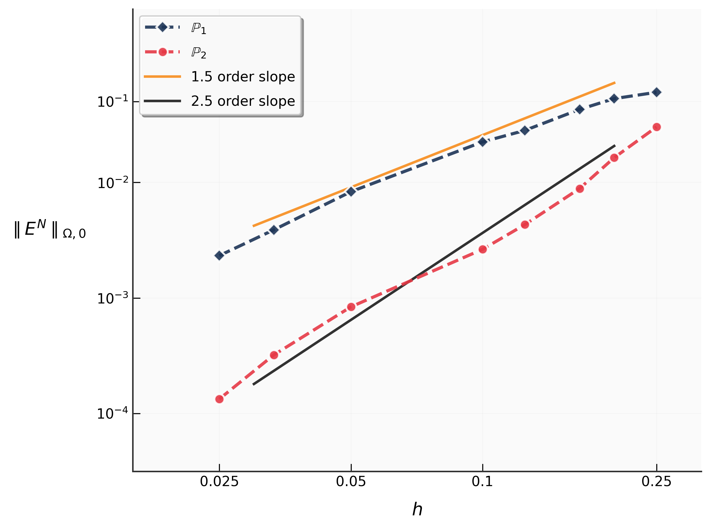
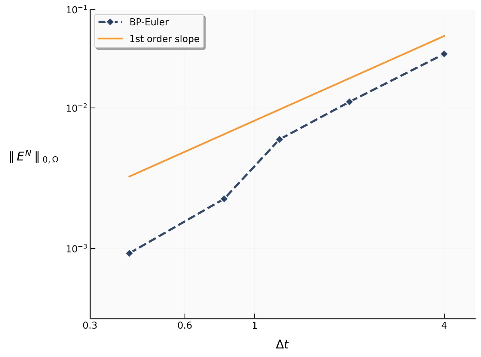
The convergence behaviour of BP–Euler is illustrated in Figure 2. In Figure 2, $\|E^{N}\|_{0,\Omega}$ denotes the norm of the difference between the exact solution and the computed solution at the final time step. In all experiments we set $T=4$. As expected, and as proved in Theorem 5.3, the Euler method exhibits first-order convergence in time.

Figure 2 presents the convergence with respect to mesh refinement for the BP–Euler method using $\mathbb{P}_{1}$ and $\mathbb{P}_{2}$ elements. We observe a convergence of approximately order $1.5$ when using $\mathbb{P}_{1}$ elements and order $2.5$ when using $\mathbb{P}_{2}$ elements. This shows that the current method also provides the $O(h^{k+1/2})$ convergence proven in [JP86] for a DG discretisation of a scalar transport equation. The proof of this fact for the CIP stabilisation is an open question, whereas an $O(h^{k+1/2})$ result for a related SUPG setting has been reported in [AHP25] in the steady-state case.

(a)

(b)

Figure 2. Left: Convergence with respect to the time step size $\Delta t$ for $\mathbb{P}_{1}$ elements with $h=1/50$. Right: Convergence with respect to the mesh size $h$ for the BP–Euler method using $\mathbb{P}_{1}$ and $\mathbb{P}_{2}$ elements with $\Delta t=1/500$.

Discontinuous solution

Next, to test the performance of the method for a problem with sharp fronts, we consider the following discontinuous inflow boundary condition:

$$\mathbf{U}_{\mathrm{in}}=\begin{cases}\mathbf{U}_{1},&0<r<\frac{1}{2},\\ \mathbf{U}_{2},&\frac{1}{2}\leq r<\frac{2}{3},\\ \mathbf{U}_{3},&\frac{2}{3}\leq r<\frac{3}{4},\\ \mathbf{U}_{4},&\frac{3}{4}\leq r<\frac{4}{5},\\ \mathbf{U}_{5},&\frac{4}{5}\leq r<\sqrt{2},\end{cases}$$

where the constant parts and their eigenvalue decompositions are given by

$$\mathbf{U}_{1}=\tfrac{1}{3}\begin{pmatrix}1&0&0\\ 0&1&0\\ 0&0&1\end{pmatrix},$$

$$\mathbf{U}_{2}=\tfrac{1}{75}\begin{pmatrix}32&24&0\\ 24&18&0\\ 0&0&25\end{pmatrix}=\tfrac{1}{5}\begin{pmatrix}4&3&0\\ 3&-4&0\\ 0&0&5\end{pmatrix}\begin{pmatrix}\tfrac{2}{3}&0&0\\ 0&0&0\\ 0&0&\tfrac{1}{3}\end{pmatrix}\tfrac{1}{5}\begin{pmatrix}4&3&0\\ 3&-4&0\\ 0&0&5\end{pmatrix},$$

$$\mathbf{U}_{3}=\tfrac{1}{3}\begin{pmatrix}1&-1&0\\ -1&1&0\\ 0&0&1\end{pmatrix}=\tfrac{1}{2}\begin{pmatrix}\sqrt{2}&\sqrt{2}&0\\ \sqrt{2}&-\sqrt{2}&0\\ 0&0&2\end{pmatrix}\begin{pmatrix}0&0&0\\ 0&\tfrac{2}{3}&0\\ 0&0&\tfrac{1}{3}\end{pmatrix}\tfrac{1}{2}\begin{pmatrix}\sqrt{2}&\sqrt{2}&0\\ \sqrt{2}&-\sqrt{2}&0\\ 0&0&2\end{pmatrix},$$

$$\mathbf{U}_{4}=\tfrac{1}{3}\begin{pmatrix}1&1&0\\ 1&1&0\\ 0&0&1\end{pmatrix}=\tfrac{1}{2}\begin{pmatrix}\sqrt{2}&\sqrt{2}&0\\ \sqrt{2}&-\sqrt{2}&0\\ 0&0&2\end{pmatrix}\begin{pmatrix}\tfrac{2}{3}&0&0\\ 0&0&0\\ 0&0&\tfrac{1}{3}\end{pmatrix}\tfrac{1}{2}\begin{pmatrix}\sqrt{2}&\sqrt{2}&0\\ \sqrt{2}&-\sqrt{2}&0\\ 0&0&2\end{pmatrix},$$

$$\mathbf{U}_{5}=\tfrac{1}{3}\begin{pmatrix}1&1&1\\ 1&1&1\\ 1&1&1\end{pmatrix}=\tfrac{\sqrt{6}}{6}\begin{pmatrix}\sqrt{2}&\sqrt{3}&1\\ \sqrt{2}&-\sqrt{3}&0\\ \sqrt{2}&0&-2\end{pmatrix}\begin{pmatrix}1&0&0\\ 0&0&0\\ 0&0&0\end{pmatrix}\tfrac{\sqrt{6}}{6}\begin{pmatrix}\sqrt{2}&\sqrt{3}&1\\ \sqrt{2}&-\sqrt{3}&0\\ \sqrt{2}&0&-2\end{pmatrix}.$$

The data are constructed such that the trace is identically equal to $1$ on the inflow boundary $\Gamma_{\text{in}}$, and the eigenvalues remain bounded between $0$ and $1$. Owing to the solenoidal velocity field, these properties are preserved throughout the domain, and thus we take $\epsilon=0$ and $\kappa=1$. The discontinuities are designed to illustrate the capability of numerical methods to handle different scenarios (see [Loh19] for more details).

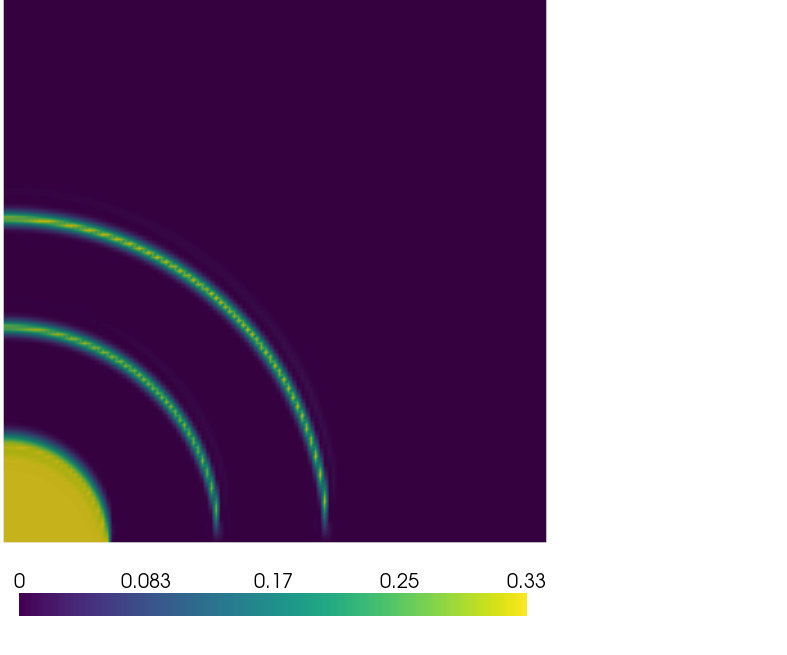
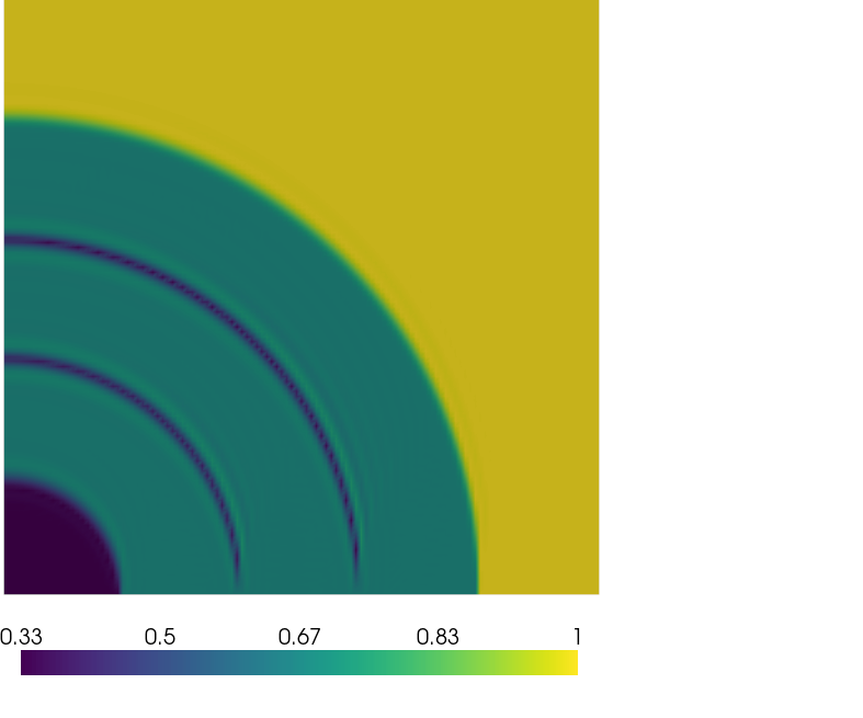
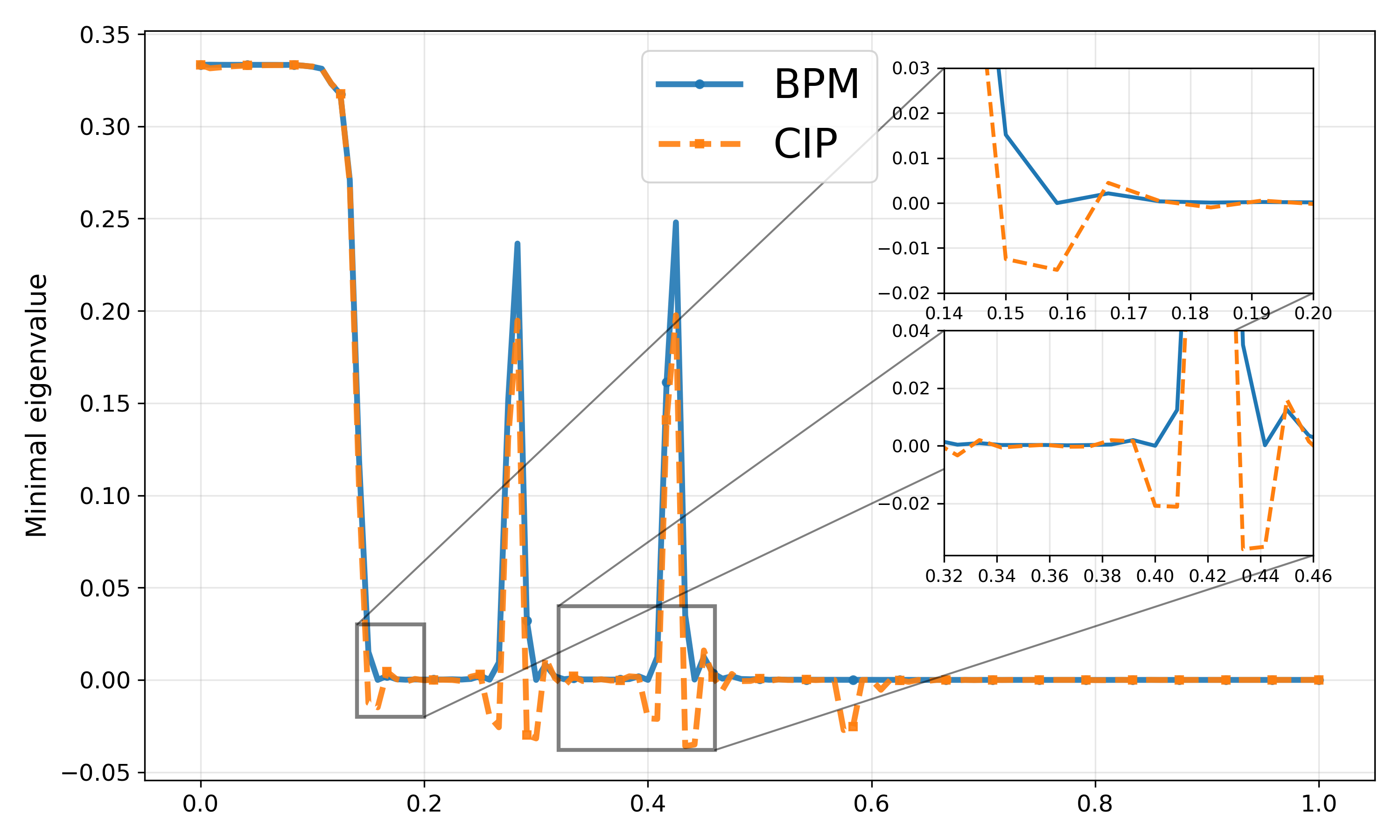
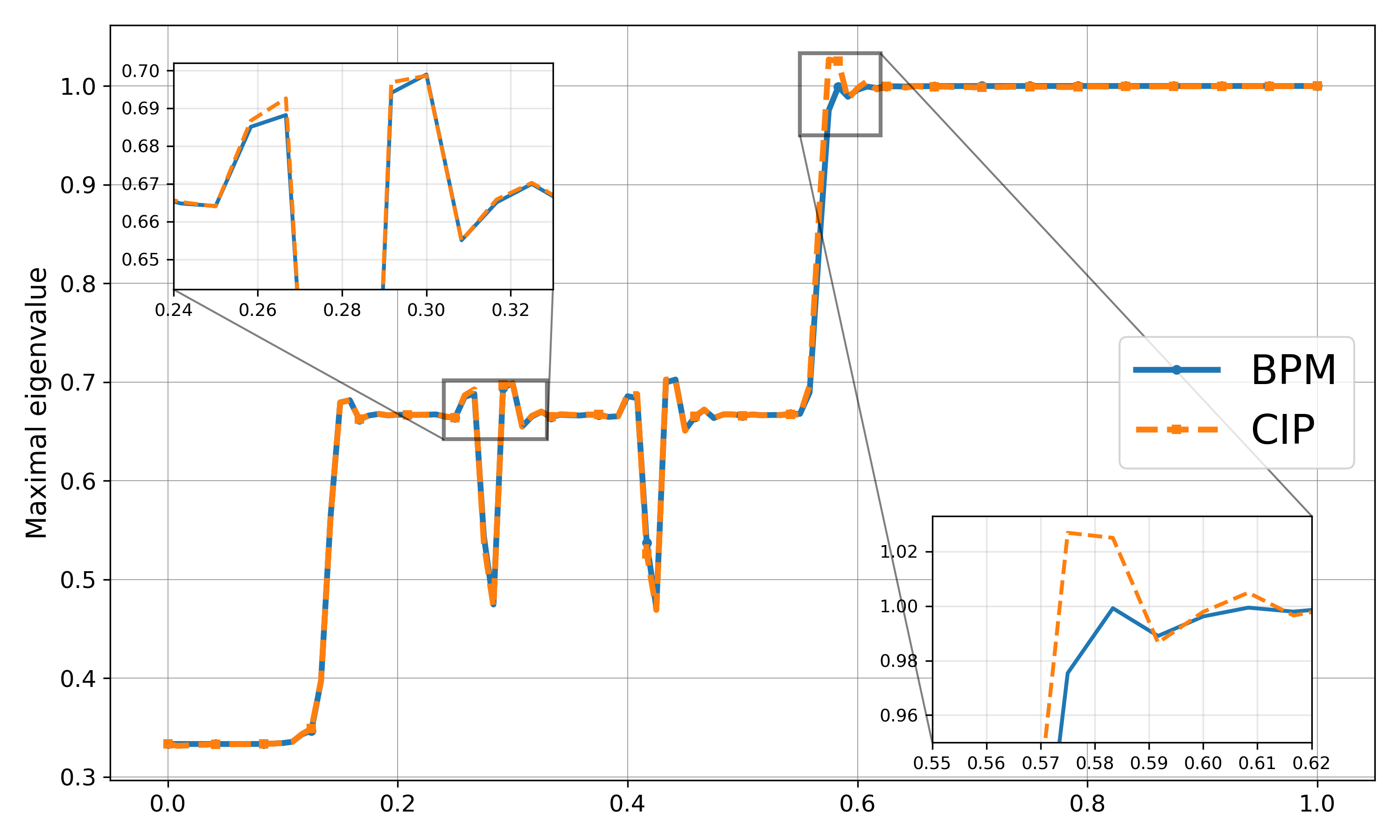
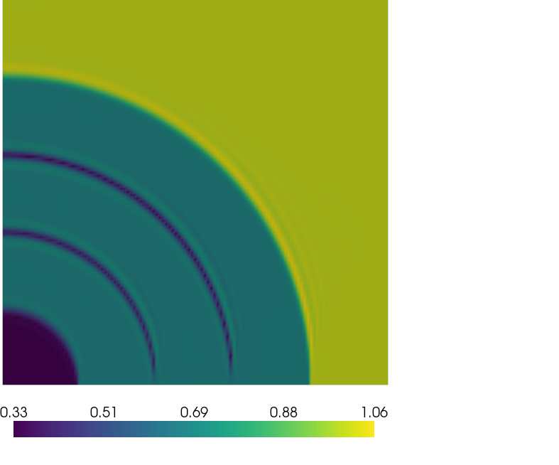
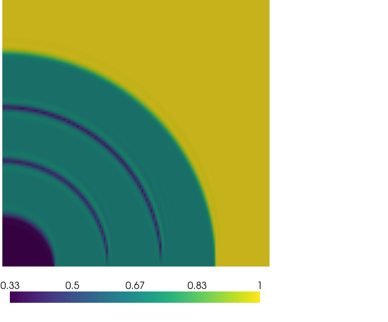
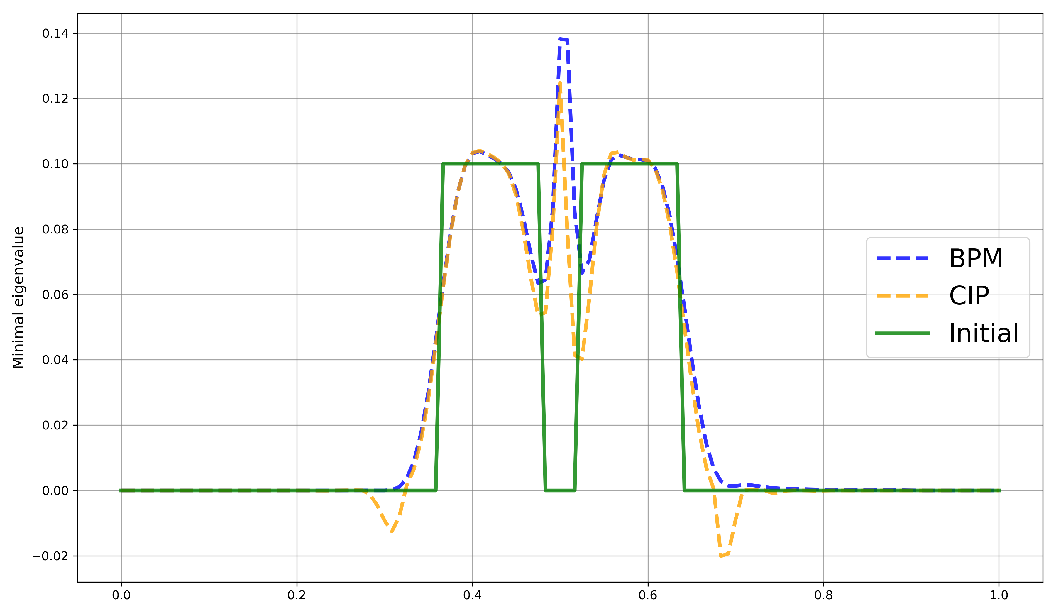
We report results for four schemes: CIP–Euler (the unconstrained baseline), BP–Euler (the bound-preserving method presented in this work), and the analogous Crank–Nicolson variants CIP–CN and BP–CN. Figure 3 shows the minimal and maximal eigenvalues obtained with the CIP–Euler and BP–Euler methods using $\mathbb{P}_{1}$ elements, together with cross-sections of these eigenvalues taken along the line $y=x$. In these experiments, we set $P=121$ and $\gamma=10^{-3}$ for the stabilisation term (25), and used a time step of $\Delta t=10^{-3}$ and $T=4$. Moreover, we choose $\omega=10^{-2}$ in the iterations of (60), which ensures very fast convergence at each time step, reaching convergence after only a few iterations.

For the CIP–Euler solution, both the minimal and maximal eigenvalues violate the bounds given by the inflow data, whereas the BP–Euler method preserves the bounds. A similar behaviour is observed for the CIP–CN and BP–CN schemes, and the corresponding $\mathbb{P}_{1}$ results are presented in Figure 4. Finally, Figure 5 reports the four schemes using quadratic elements ($k=2$), together with the corresponding cross-sections along $y=x$. The same conclusions hold for $\mathbb{P}_{2}$ elements. In particular, although the admissibility constraints are imposed only at the nodes, the plotted eigenvalues remain within $[0,1]$ also between the nodes in these tests.

(a) Minimal eigenvalue for the CIP–Euler solution.

(b) Maximal eigenvalue for the CIP–Euler solution.

(c) Minimal eigenvalue for the BP–Euler solution.

(d) Maximal eigenvalue for the BP–Euler solution.

(e) Cross-section of the minimal eigenvalue along $y=x$.

(f) Cross-section of the maximal eigenvalue along $y=x$.

Figure 3. Solution of (62) at $T=4$ with discontinuous inflow data: minimal and maximal eigenvalues obtained with the CIP–Euler and BP–Euler schemes, together with cross-sections taken along $y=x$ ($\mathbb{P}_{1}$ elements).

(a) Minimal eigenvalue for the CIP–CN solution.

(b) Maximal eigenvalue for the CIP–CN solution.

(c) Minimal eigenvalue for the BP–CN solution.

(d) Maximal eigenvalue for the BP–CN solution.

(e) Cross-section of the minimal eigenvalue along $y=x$.

(f) Cross-section of the maximal eigenvalue along $y=x$.

Figure 4. Solution of (62) at $T=4$ with discontinuous inflow data: minimal and maximal eigenvalues obtained with the CIP–CN and BP–CN schemes, together with cross-sections taken along $y=x$ ($\mathbb{P}_{1}$ elements).

(a) Minimal eigenvalue for the CIP–Euler solution.

(b) Maximal eigenvalue for the CIP–Euler solution.

(c) Minimal eigenvalue for the BP–Euler solution.

(d) Maximal eigenvalue for the BP–Euler solution.

(e) Cross-section of the minimal eigenvalue along $y=x$.

(f) Cross-section of the maximal eigenvalue along $y=x$.

Figure 5. Solution of (62) at $T=4$ with discontinuous inflow data: minimal and maximal eigenvalues obtained with the CIP–Euler and BP–Euler schemes, together with cross-sections taken along $y=x$ ($\mathbb{P}_{2}$ elements).

Example 2.

(Solid body rotation): We then test the method in a modified version of the solid body rotation benchmark originally proposed in [Zal79] and later extended in [Lev96]. In [Loh17], this benchmark was further extended to the case where the unknown is a $3\times 3$ tensor defined on the two-dimensional domain $\Omega=(0,1)^{2}$ under the stationary, divergence-free velocity field

(63) $${\boldsymbol{\beta}}=\left(\tfrac{1}{2}-y,x-\tfrac{1}{2}\right)^{T}.$$

Since for this test we consider $\mathcal{D}=\mathbf{0}$ and $\mu=0$, after one full rotation, corresponding to $T=2\pi$, the exact solution returns to the initial condition. Thus, the quality of the numerical solution is assessed by comparing the numerical solution at $t=T$ with the initial data.

The initial condition is defined as

(64) $$\mathbf{U}_{0}(x,y):=\begin{cases}\mathbf{U}^{(1)}&\text{if }\sqrt{(x-0.25)^{2}+(y-0.5)^{2}}\leq 0.15,\quad\text{`hump'},\\ \mathbf{U}^{(2)}&\text{if }\sqrt{(x-0.5)^{2}+(y-0.25)^{2}}\leq 0.15,\quad\text{`cone'},\\ \mathbf{U}^{(3)}&\text{if }\sqrt{(x-0.75)^{2}+(y-0.5)^{2}}\leq 0.15,\quad\text{`semi-ellipse'},\\ \mathbf{U}^{(4)}&\text{if }\sqrt{(x-0.5)^{2}+(y-0.75)^{2}}\leq 0.15,\quad\text{`slotted cylinder'},\\ \mathbf{0}&\text{otherwise},\end{cases}$$

which consists of four functions defined on circles centred at different points. In what follows we use the shorthand $r:=\sqrt{x^{2}+y^{2}}$. The positive semidefinite tensors $\mathbf{U}^{(1)}$, $\mathbf{U}^{(2)}$, $\mathbf{U}^{(3)}$ and $\mathbf{U}^{(4)}$ are specified through their eigenvalue decompositions as follows:

$$\mathbf{U}^{(1)}(x,y):=\begin{pmatrix}1&0&0\\ 0&\cos\phi&\sin\phi\\ 0&\sin\phi&-\cos\phi\end{pmatrix}\frac{1}{r}\begin{pmatrix}x&y&0\\ y&-x&0\\ 0&0&r\end{pmatrix}\begin{pmatrix}u_{1}^{(1)}&0&0\\ 0&u_{2}^{(1)}&0\\ 0&0&u_{3}^{(1)}\end{pmatrix}\frac{1}{r}\begin{pmatrix}x&y&0\\ y&-x&0\\ 0&0&r\end{pmatrix}\begin{pmatrix}1&0&0\\ 0&\cos\phi&\sin\phi\\ 0&\sin\phi&-\cos\phi\end{pmatrix},$$

where

$$u_{1}^{(1)}=\left(\frac{1}{2}(1+\cos(\pi r))\right)^{3},\quad u_{2}^{(1)}=\left(\frac{1}{2}(1+\cos(\pi r))\right)^{2},\quad u_{3}^{(1)}=\frac{1}{2}(1+\cos(\pi r)),\quad\phi=\frac{1}{2}\operatorname{atan2}(x,y),$$

$$\mathbf{U}^{(2)}(x,y):=\frac{1}{10}\begin{pmatrix}10&0&0\\ 0&8&6\\ 0&6&-8\end{pmatrix}\frac{1}{r}\begin{pmatrix}x&y&0\\ y&-x&0\\ 0&0&r\end{pmatrix}\begin{pmatrix}u_{1}^{(2)}&0&0\\ 0&u_{a}^{(2)}&0\\ 0&0&u_{b}^{(2)}\end{pmatrix}\frac{1}{r}\begin{pmatrix}x&y&0\\ y&-x&0\\ 0&0&r\end{pmatrix}\frac{1}{10}\begin{pmatrix}10&0&0\\ 0&8&6\\ 0&6&-8\end{pmatrix},$$

where $u^{(2)}_{1}=\frac{1}{2}-\frac{1}{2}r$, $u^{(2)}_{a}=\frac{1}{2}-\frac{1}{2}|x|$, and $u^{(2)}_{b}=1-r$,

(65) $$\mathbf{U}^{(3)}(x,y):=\begin{pmatrix}u^{(3)}_{1}&0&0\\ 0&u^{(3)}_{1}&0\\ 0&0&u^{(3)}_{1}\end{pmatrix},$$

where

$$u_{1}^{(3)}=u_{2}^{(3)}=u_{3}^{(3)}=\sqrt{1-r^{2}},$$

$$\mathbf{U}^{(4)}(x,y):=\begin{cases}\frac{1}{10}\begin{pmatrix}-8&6&0\\ 6&8&0\\ 0&0&10\end{pmatrix}\begin{pmatrix}u_{3}^{(4)}&0&0\\ 0&u_{1}^{(4)}&0\\ 0&0&u_{2}^{(4)}\end{pmatrix}\frac{1}{10}\begin{pmatrix}-8&6&0\\ 6&8&0\\ 0&0&10\end{pmatrix},&(|x|\geq\frac{1}{6}\vee y\geq\frac{2}{3})\wedge(x>0),\\[5.69046pt] \frac{1}{10}\begin{pmatrix}-8&6&0\\ 6&8&0\\ 0&0&10\end{pmatrix}\begin{pmatrix}u_{3}^{(4)}&0&0\\ 0&u_{3}^{(4)}&0\\ 0&0&u_{2}^{(4)}\end{pmatrix}\frac{1}{10}\begin{pmatrix}-8&6&0\\ 6&8&0\\ 0&0&10\end{pmatrix},&(|x|\geq\frac{1}{6}\vee y\geq\frac{2}{3})\wedge(x<0),\\[5.69046pt] \mathbf{0},&\text{elsewhere},\end{cases}$$

where

$$u_{1}^{(4)}=0.1,\quad u_{2}^{(4)}=0.45,\quad u_{3}^{(4)}=1.$$

The intermediate and largest eigenvalues of $\mathbf{U}^{(2)}$ are given by

$$u_{2}^{(2)}=\begin{cases}u_{a}^{(2)},&|x|\geq 2r-1,\\ u_{b}^{(2)},&|x|<2r-1,\end{cases}\hskip 28.45274ptu_{3}^{(2)}=\begin{cases}u_{b}^{(2)},&|x|\geq 2r-1,\\ u_{a}^{(2)},&|x|<2r-1.\end{cases}$$

The minimal and maximal eigenvalues of $\mathbf{U}_{0}$ are $0$ and $1$, respectively. Thus, we take $\epsilon=0$ and $\kappa=1$.

The labels hump, cone, semi-ellipse and slotted cylinder correspond to the design of the respective minimal and maximal eigenvalues, reflecting their similarity to the scalar solid-body rotation benchmark. The bodies undergo a counter-clockwise rotation, completing one full revolution at $t=2\pi$. For the space discretisation in this example, we employ piecewise linear elements (that is, $k=1$). We set $P=121$, which yields a uniform grid with $2\times 121\times 121$ mesh cells, and use a time step of $\Delta t=5\times 10^{-4}$. In all experiments in this example we use $\omega=0.01$ in the iterative method (60) and $\gamma=10^{-3}$ in the stabilisation term (25).

Figure 6 illustrates the minimal and maximal eigenvalues of the initial data (64). Figure 7 presents the minimal and maximal eigenvalues of the numerical solution obtained by BP–Euler and CIP–Euler at the final time $t=T$. To compare the performance of these two approaches, we consider a cross-section along the line $y=0.8$ extracted from both the minimal and maximal eigenvalues of the initial data (64) and from the corresponding numerical solutions. This comparison enables us to assess how effectively the bound-preserving method prevents overshoots and undershoots compared to the CIP method. From the eigenvalue plots and cross-sections, it is evident that the BP method successfully enforces the lower and upper bounds on the eigenvalues of the solution. In the cross-section plots, initial denotes the eigenvalues of the initial datum.

Figure 8 presents analogous results for the BP–CN and CIP–CN schemes. While BP–CN ensures that the solution remains within the physical bounds, CIP–CN may exhibit violations of these bounds, as is evident in both the eigenvalue plots and the cross-sections at $y=0.8$.

(a) Minimal eigenvalue of the initial datum.

(b) Maximal eigenvalue of the initial datum.

Figure 6. Minimal and maximal eigenvalues of the initial datum (64).

(a) Minimal eigenvalue for the CIP–Euler solution.

(b) Maximal eigenvalue for the CIP–Euler solution.

(c) Minimal eigenvalue for the BP–Euler solution.

(d) Maximal eigenvalue for the BP–Euler solution.

(e) Cross-section of the minimal eigenvalue along $y=0.8$.

(f) Cross-section of the maximal eigenvalue along $y=0.8$.

Figure 7. Example 2 at $t=T=2\pi$: minimal and maximal eigenvalues obtained with the CIP–Euler and BP–Euler schemes, together with cross-sections along $y=0.8$.

(a) Minimal eigenvalue for the CIP–CN solution.

(b) Maximal eigenvalue for the CIP–CN solution.

(c) Minimal eigenvalue for the BP–CN solution.

(d) Maximal eigenvalue for the BP–CN solution.

(e) Cross-section of the minimal eigenvalue along $y=0.8$.

(f) Cross-section of the maximal eigenvalue along $y=0.8$.

Figure 8. Example 2 at $t=T=2\pi$: minimal and maximal eigenvalues obtained with the CIP–CN and BP–CN schemes, together with cross-sections along $y=0.8$.

7. Conclusions and outlook

In this work we have extended the nodally bound-preserving idea to the numerical approximation of time-dependent tensor-valued partial differential equations. The method is built using a variational inequality posed over a set of acceptable functions, which is proven to be well-posed, and yielding to an unconditionally stable and optimally-convergent discretisation. Our approach offers several advantages over existing methods. Unlike post-processing techniques, our method directly enforces the eigenvalue constraints as part of the variational formulation, ensuring that the discrete solution satisfies the physical constraints at the degrees of freedom at each time step. In contrast to transformation-based approaches, our method maintains a linear structure for linear problems in the unconstrained limit, and in the sense that the baseline discretisation remains linear, simplifying both the analysis and implementation. Moreover, the CIP stabilisation provides robustness in the convection-dominated regime without compromising accuracy in diffusion-dominated regions through its consistent interior penalty formulation.

There are still several questions that remain open. For example, the extension of the analysis to higher-order time discretisations, exploring the possibility of combining the current method with IMEX-type schemes for nonlinear problems, and whether this framework can be extended to nonlinear conservation laws are very interesting open questions that will be subject of future research.

References

• [AA21] Abdolreza Amiri and Ioannis K Argyros. On the approximation of mth power divided differences preserving the local order of convergence. Applied Mathematics and Computation, 410:126415, 2021.
• [ABP24] Abdolreza Amiri, Gabriel R. Barrenechea, and Tristan Pryer. A nodally bound-preserving finite element method for reaction–convection–diffusion equations. Mathematical Models and Methods in Applied Sciences, 34(08):1533–1565, 2024.
• [ABP25] Abdolreza Amiri, Gabriel R. Barrenechea, and Tristan Pryer. A nodally bound-preserving finite element method for time-dependent convection–diffusion equations. Journal of Computational and Applied Mathematics, page 116691, 2025.
• [AFPA06] V. Arsigny, P. Fillard, X. Pennec, and N. Ayache. Log-euclidean metrics for fast and simple calculus on diffusion tensors. Magnetic Resonance in Medicine, 56(2):411–421, 2006.
• [AHP25] Ben S Ashby, Abdalaziz Hamdan, and Tristan Pryer. A nodally bound-preserving finite element method for hyperbolic convection-reaction problems. arXiv preprint arXiv:2501.11042, 2025.
• [AP25] Ben S Ashby and Tristan Pryer. Discretisation of an Oldroyd-B viscoelastic fluid flow using a Lie derivative formulation. Advances in Computational Mathematics, 51(1):1, 2025.
• [BBK17] Gabriel R. Barrenechea, Erik Burman, and Fotini Karakatsani. Edge-based nonlinear diffusion for finite element approximations of convection-diffusion equations and its relation to algebraic flux-correction schemes. Numer. Math., 135(2):521–545, 2017.
• [BDD+23] Igor A. Baratta, Joseph P. Dean, Jørgen S. Dokken, Michal Habera, Jack S. Hale, Chris N. Richardson, Marie E. Rognes, Matthew W. Scroggs, Nathan Sime, and Garth N. Wells. Dolfinx: A new finite element computing platform, 2023.
• [BE05] Erik Burman and Alexandre Ern. Stabilized Galerkin approximation of convection-diffusion-reaction equations: discrete maximum principle and convergence. Math. Comp., 74(252):1637–1652 (electronic), 2005.
• [BF09] Erik Burman and Miguel A. Fernández. Finite element methods with symmetric stabilization for the transient convection–diffusion–reaction equation. Computer Methods in Applied Mechanics and Engineering, 198(33-36):2508–2519, 2009.
• [BGPV24] Gabriel R. Barrenechea, Emmanuil H. Georgoulis, Tristan Pryer, and Andreas Veeser. A nodally bound-preserving finite element method. IMA J. Numer. Anal., 44(4):2198–2219, 2024.
• [BH04] Erik Burman and Peter Hansbo. Edge stabilization for Galerkin approximations of convection–diffusion–reaction problems. Computer Methods in Applied Mechanics and Engineering, 193(15-16):1437–1453, 2004.
• [BJK25] Gabriel R. Barrenechea, Volker John, and Petr Knobloch. Monotone Discretizations for Elliptic Second Order Partial Differential Equations. Springer Cham, 2025.
• [BKK08] Jan H Brandts, Sergey Korotov, and Michal Křížek. The discrete maximum principle for linear simplicial finite element approximations of a reaction–diffusion problem. Linear Algebra and its Applications, 429(10):2344–2357, 2008.
• [BML94] P. J. Basser, J. Mattiello, and D. LeBihan. MR diffusion tensor spectroscopy and imaging. Biophysical Journal, 66(1):259–267, 1994.
• [BPT25] Gabriel R. Barrenechea, Tristan Pryer, and Alex Trenam. A nodally bound-preserving discontinuous galerkin method for the drift–diffusion equation. Journal of Computational and Applied Mathematics, page 116670, 2025.
• [BS08] S. C. Brenner and L. R. Scott. The Mathematical Theory of Finite Element Methods, volume 15 of Texts in Applied Mathematics. Springer, New York, 3rd edition, 2008.
• [CHQZ07] C. Canuto, M. Y. Hussaini, A. Quarteroni, and T. A. Zang. Spectral Methods: Fundamentals in Single Domains. Springer, Berlin, 2007.
• [CR73] P. G. Ciarlet and P.-A. Raviart. Maximum principle and uniform convergence for the finite element method. Comput. Methods Appl. Mech. Engrg., 2:17–31, 1973.
• [dGP93] P. G. de Gennes and J. Prost. The Physics of Liquid Crystals. Oxford University Press, Oxford, 2nd edition, 1993.
• [EG21] Alexandre Ern and Jean-Luc Guermond. Finite Elements I. Springer, 2021.
• [EHS09] John A. Evans, Thomas J. R. Hughes, and Giancarlo Sangalli. Enforcement of constraints and maximum principles in the variational multiscale method. Comput. Methods Appl. Mech. Engrg., 199(1-4):61–76, 2009.
• [FK04] Raanan Fattal and Raz Kupferman. Constitutive laws for the matrix-logarithm of the conformation tensor. Journal of Non-Newtonian Fluid Mechanics, 123(2):281–285, 2004.
• [GMP15] Jan Giesselmann, Charalambos Makridakis, and Tristan Pryer. A posteriori analysis of discontinuous galerkin schemes for systems of hyperbolic conservation laws. SIAM Journal on Numerical Analysis, 53(3):1280–1303, 2015.
• [GNPY14] Jean-Luc Guermond, Murtazo Nazarov, Bojan Popov, and Yong Yang. A second-order maximum principle preserving lagrange finite element technique for nonlinear scalar conservation equations. SIAM Journal on Numerical Analysis, 52(4):2163–2182, 2014.
• [GP16a] Jan Giesselmann and Tristan Pryer. Reduced relative entropy techniques for a priori analysis of multiphase problems in elastodynamics. BIT Numerical Mathematics, 56(1):99–127, 2016.
• [GP16b] Jean-Luc Guermond and Bojan Popov. Invariant domains and first-order continuous finite element approximation for hyperbolic systems. SIAM Journal on Numerical Analysis, 54(4):2466–2489, 2016.
• [GPT19] Jean-Luc Guermond, Bojan Popov, and Ignacio Tomas. Invariant domain preserving discretization-independent schemes and convex limiting for hyperbolic systems. Computer Methods in Applied Mechanics and Engineering, 347:143–175, 2019.
• [HR90] John G Heywood and Rolf Rannacher. Finite-element approximation of the nonstationary Navier–Stokes problem. part iv: error analysis for second-order time discretization. SIAM Journal on Numerical Analysis, 27(2):353–384, 1990.
• [Hub07] Matthew Hubbard. Non-oscillatory third order fluctuation splitting schemes for steady scalar conservation laws. Journal of Computational Physics, 222(2):740–768, 2007.
• [Hug12] Thomas J. R. Hughes. The Finite Element Method: Linear Static and Dynamic Finite Element Analysis. Dover Publications, Mineola, NY, 2nd edition, 2012.
• [JP86] Claes Johnson and Juhani Pitkäranta. An analysis of the discontinuous Galerkin method for a scalar hyperbolic equation. Mathematics of Computation, 46(173):1–26, 1986.
• [Kik77] Fumio Kikuchi. Discrete maximum principle and artificial viscosity in finite element approximations to convective diffusion equations. Tokyo, University, Institute of Space and Aeronautical Science, Report no. 550, 42:153–166, 1977.
• [Kor76] G. M. Korpelevich. Iterative methods for variational inequalities. Ekonomika i Matematicheskie Metody, 12:747–756, 1976. Russian publication - English translation may exist.
• [KS00] David Kinderlehrer and Guido Stampacchia. An introduction to variational inequalities and their applications. SIAM, 2000.
• [KS24a] Brendan Keith and Thomas M Surowiec. Proximal Galerkin: A structure-preserving finite element method for pointwise bound constraints. Foundations of Computational Mathematics, pages 1–97, 2024.
• [KS24b] Robert C Kirby and Daniel Shapero. High-order bounds-satisfying approximation of partial differential equations via finite element variational inequalities. Numerische Mathematik, 156(3):927–947, 2024.
• [Kuz07] Dmitri Kuzmin. Algebraic flux correction for finite element discretizations of coupled systems. In M. Papadrakakis, E. Oñate, and B. Schrefler, editors, Proceedings of the Int. Conf. on Computational Methods for Coupled Problems in Science and Engineering, pages 1–5. CIMNE, Barcelona, 2007.
• [Lev96] Randall J Leveque. High-resolution conservative algorithms for advection in incompressible flow. SIAM Journal on Numerical Analysis, 33(2):627–665, 1996.
• [LeV02] Randall J. LeVeque. Finite Volume Methods for Hyperbolic Problems. Cambridge University Press, Cambridge, 2002.
• [LM12] Jacques Louis Lions and Enrico Magenes. Non-homogeneous boundary value problems and applications: Vol. 1, volume 181. Springer Science & Business Media, 2012.
• [Loh17] Christoph Lohmann. Flux-corrected transport algorithms preserving the eigenvalue range of symmetric tensor quantities. Journal of Computational Physics, 350:907–926, 2017.
• [Loh19] Christoph Lohmann. Algebraic flux correction schemes preserving the eigenvalue range of symmetric tensor fields. ESAIM: Mathematical Modelling and Numerical Analysis, 53(3):833–867, 2019.
• [MH85] Akira Mizukami and Thomas J. R. Hughes. A Petrov-Galerkin finite element method for convection-dominated flows: an accurate upwinding technique for satisfying the maximum principle. Comput. Methods Appl. Mech. Engrg., 50(2):181–193, 1985.
• [Moa05] M. Moakher. A differential geometric approach to the geometric mean of symmetric positive-definite matrices. SIAM Journal on Matrix Analysis and Applications, 26(3):735–747, 2005.
• [OP02] R. G. Owens and T. N. Phillips. Computational Rheology. Imperial College Press, London, 2002.
• [SDRW23] Matthew W. Scroggs, Jørgen S. Dokken, Chris N. Richardson, and Garth N. Wells. Dolfinx: The next generation fenics problem solving environment. Zenodo, 2023.
• [SH92] J. C. Simo and T. J. R. Hughes. Computational inelasticity. Interdisciplinary Applied Mathematics, 7, 1992.
• [Zal79] Steven T Zalesak. Fully multidimensional flux-corrected transport algorithms for fluids. Journal of computational physics, 31(3):335–362, 1979.
• [ZS10] Xiangxiong Zhang and Chi-Wang Shu. On positivity-preserving high order discontinuous galerkin schemes for compressible euler equations on rectangular meshes. Journal of Computational Physics, 229(23):8918–8934, 2010.
• [ZS11] Xiangxiong Zhang and Chi-Wang Shu. Positivity-preserving high order discontinuous galerkin schemes for compressible euler equations with source terms. Journal of Computational Physics, 230(4):1238–1248, 2011.