AI-exposed jobs deteriorated before ChatGPT

M. R. Frank^1,2,3∗, A. Javadian Sabet¹, L. Simon⁴, S. H. Bana^2,5, R. Yu^6,7 ¹Department of Informatics and Networked Systems, University of Pittsburgh, Pittsburgh, PA 15215, USA. ²Digital Economy Lab, Stanford University, Stanford, CA 94305, USA. ³AI Economy Institute, Microsoft, Redmond, WA 98052, USA. ⁴Revelio Labs, New York, NY 10010, USA. ⁵Argyros College of Business and Economics, Chapman University, Orange, CA, 92866, USA. ⁶Teachers College, Columbia University, New York, NY, 10027, USA. ⁷Data Science Institute, Columbia University, New York, NY, 10027, USA ^∗Corresponding author. Email: mrfrank@pitt.edu

Abstract

Public debate links worsening job prospects for AI-exposed occupations to the release of ChatGPT in late 2022. Using monthly U.S. unemployment insurance records, we measure occupation- and location-specific unemployment risk and find that risk rose in AI-exposed occupations beginning in early 2022, months before ChatGPT. Analyzing millions of LinkedIn profiles, we show that graduate cohorts from 2021 onward entered AI-exposed jobs at lower rates than earlier cohorts, with gaps opening before late 2022. Finally, from millions of university syllabi, we find that graduates taking more AI-exposed curricula had higher first-job pay and shorter job searches after ChatGPT. Together, these results point to forces pre-dating generative AI and to the ongoing value of LLM-relevant education.

Many observers worry that college-educated workers are disproportionately exposed to generative AI–driven task automation (?, ?) and thus face job displacement as these tools diffuse ¹¹1“Anthropic CEO warns AI could eliminate half of all entry-level white-collar jobs”. Fortune Magazine (May 28, 2025). Timing is a key implication of this hypothesis: if deteriorating labor-market outcomes in 2022–2024 were driven primarily by large language models (LLMs), then the sharpest deterioration should occur after the mass-market emergence of LLM applications. ChatGPT—launched in November 2022 and rapidly adopted by consumers (?)—provides a salient inflection point for the broader diffusion of LLM services (e.g., including Claude, Copilot, and Gemini). And, consistent with employment concerns, early-career workers in LLM-exposed occupations experienced an employment decline (?, ?) and/or decreasing salaries (?) while recent college graduates experience elevated unemployment (?) during this period. If these poor outcomes are because of LLM automation, then perhaps teaching LLM-exposed skills fails to prepare students for the US labor market.

However, other studies find little impact from LLM’s on workers’ wages or hours worked (?), and other macroeconomic and sector-specific forces were already shifting in early 2022 contributing to weakening outcomes in the same AI-exposed occupations. For example, monetary tightening accelerated through 2022–2023 (?) and may have impacted job stability (?). Also, job postings for software developers declined markedly over 2022–2023 (?) perhaps as a correction to increased hiring during pandemic years (?). Instead of LLM diffusion, if such forces were central drivers, then deterioration could be detectable before ChatGPT’s launch.

To clarify the origins and timing of these changes, we integrate three large-scale datasets spanning administrative unemployment records, online career histories, and university curricula. First, using monthly unemployment insurance claims linked to occupations and states, we construct a monthly measure of unemployment risk and find that risk rose for LLM exposed occupations beginning in early 2022—months before ChatGPT. Throughout, we define an occupation’s AI or LLM exposure using existing exposure estimates (?) according to the share of its workplace tasks in the Bureau of Labor Statistics (BLS) O*NET database that could be affected by LLMs with simple interfaces and general training. Second, analyzing millions of LinkedIn profiles from Revelio Labs, we show that graduate cohorts from 2021 onward entered LLM exposed jobs at lower rates than earlier cohorts with these gaps opening prior to late 2022. Finally, using millions of university course syllabi (?), we measure graduates’ educational exposure to LLM-related content and find that higher exposure predicts higher first-job salaries and shorter job searches after ChatGPT. Together, these results separate pre-existing labor-market weakening from later LLM diffusion and underscore the ongoing value of LLM-relevant skill development during higher education. These findings warn against using ChatGPT’s 2022 launch as a clean natural experiment and argue that education/workforce programs should keep AI-exposed skills (e.g., writing, coding, information synthesis).

Unemployment risk for AI-exposed occupations

We first focus on unemployment for the workers of AI exposed occupations that are most likely to experience change because of AI automation. When considering major occupation groups (i.e., two-digit Standard Occupation Classification (SOC) codes), we consider the average exposure of more detailed occupations (i.e., six-digit SOC codes) contained in that occupation group (note: we consider LLM exposure by six-digit SOC codes in all other analyses). Next we incorporate monthly administrative records from the ETA 203 report from the Employment and Training Administration (ETA) within the U.S. Department of Labor. This report aggregates monthly data from each U.S. state’s unemployment insurance program detailing the most recent major occupation group of each continuing claimant. After combining with annual occupation employment data from the BLS Occupational Employment and Wage Statistics (OEWS) program, we calculate an occupation’s unemployment risk (?) representing the probability of claiming unemployment in each state each month given a worker’s occupation (see details in Supplementary Materials Unemployment Risk).

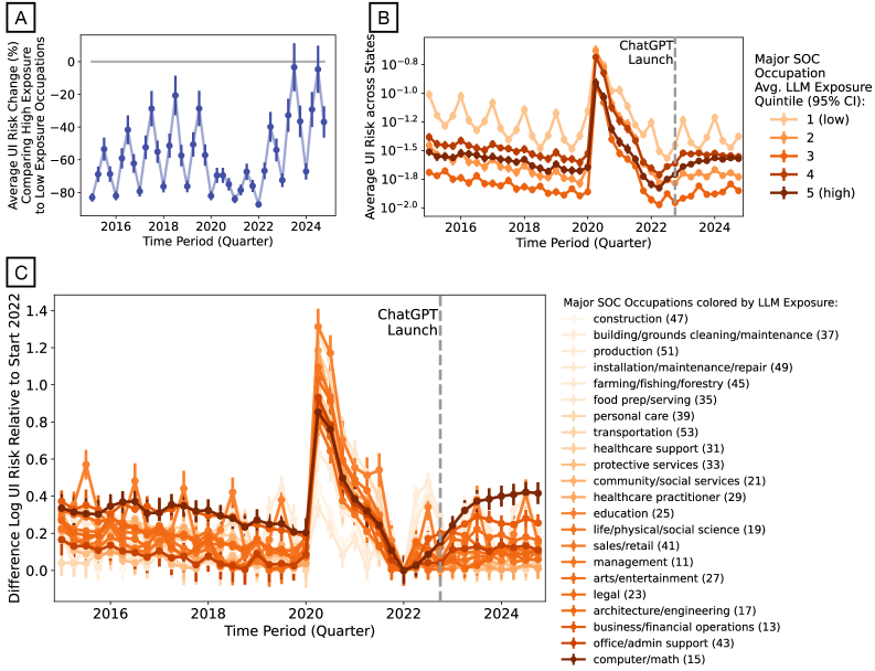
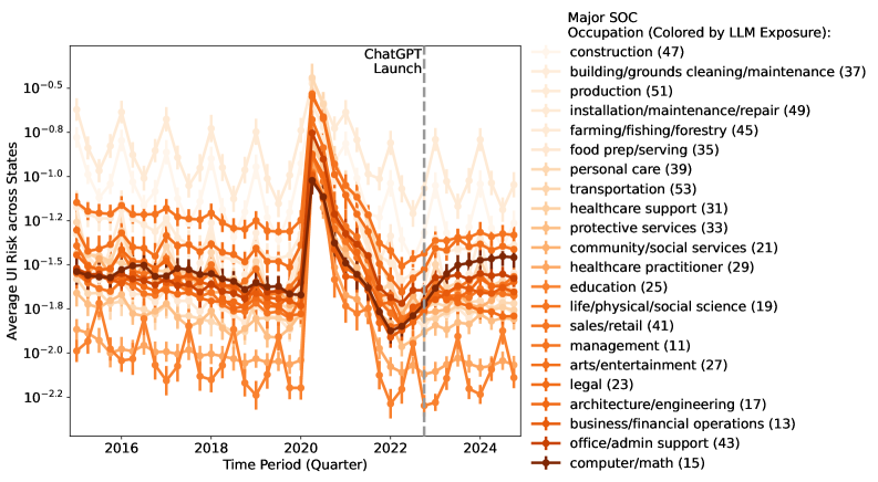
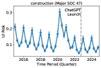
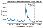
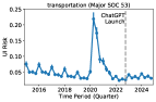
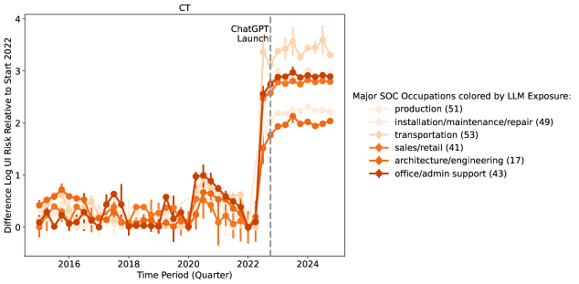
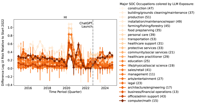
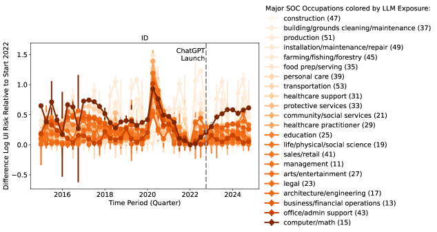
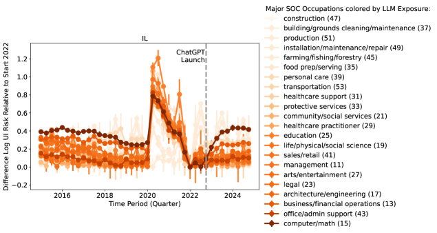
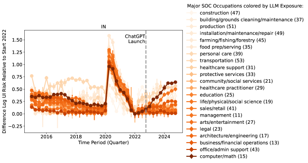
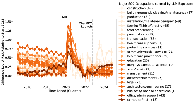
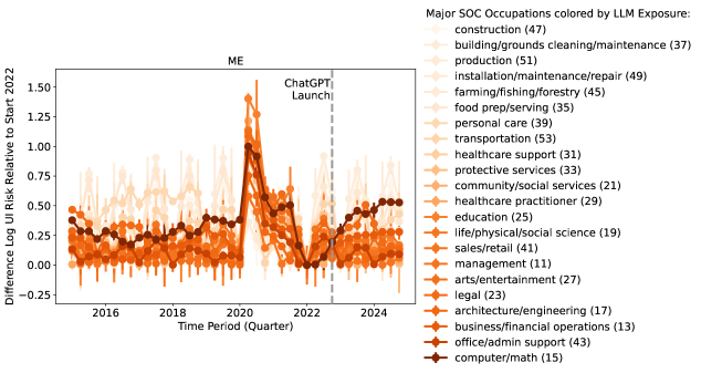
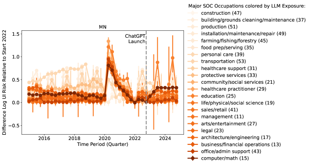
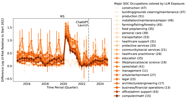
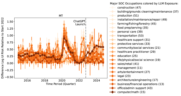
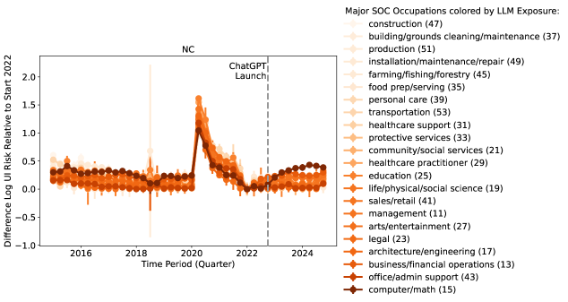
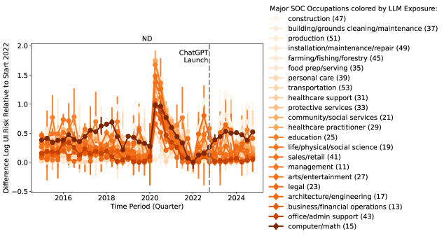
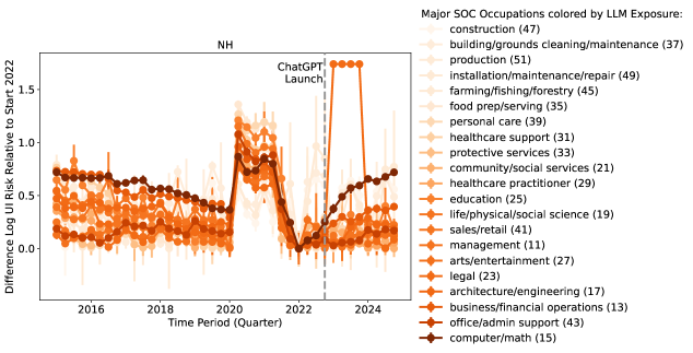
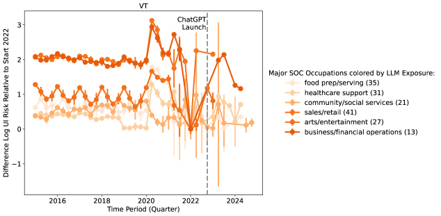
Refer to caption — Figure 1: Unemployment risk for AI (LLM) exposed workers increased starting before the launch of ChatGPT. (A) Unemployment risk for occupations with high exposure compared to occupations with low exposure (see SI Fig. S2 for seasonally-adjusted plot). (B) Unemployment risk for occupations grouped into exposure quintiles. (C) Unemployment risk relative to first quarter 2022 by major occupation. Lines are colored by major occupation’s AI-exposure. We compute unemployment risk monthly across states and report quarterly series as the mean of monthly values across all states within each quarter (see SI Fig. S3 for non-normalized version).

Typically, unemployment risk is 20-80% lower in LLM-exposed occupations (e.g., computer/mathematical) compared to less exposed occupations (e.g., construction; Fig. 1A). This gap widens during 2020–2021, consistent with pandemic-era differences in the ability to work remotely. Beginning in early 2022, however, the gap narrows sharply with some quarters of 2023-2024 exhibiting no difference between high- and low-exposure groups.

Is this deterioration because exposed occupations have more unemployment risk after the launch of ChatGPT? We group occupations into quintiles of LLM exposure and plot average unemployment risk over time (Fig. 1B). Across the period, lower-exposure quintiles exhibit higher levels and stronger seasonality, while all quintiles show a pandemic spike in 2020 followed by a trough in early 2022. Importantly, unemployment risk in the most exposed quintiles begins rising after this early-2022 trough—well before ChatGPT’s November 2022 launch—and then stabilizes rather than accelerating in the quarters following the launch.

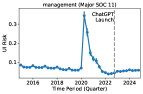
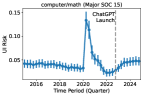
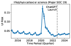
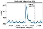
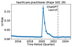
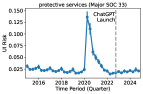
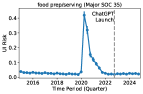
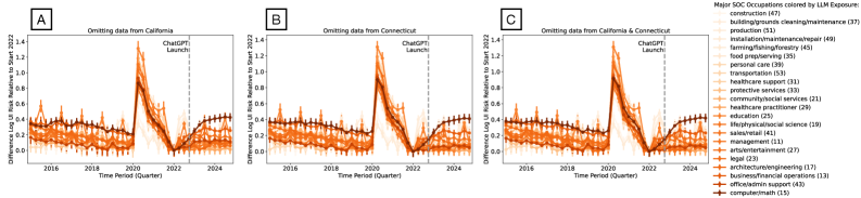
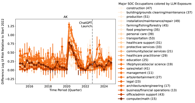
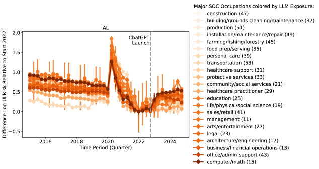
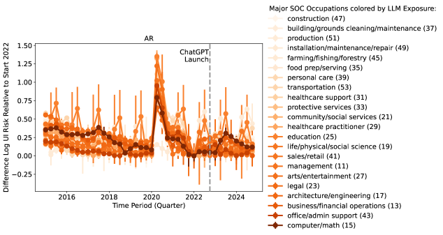
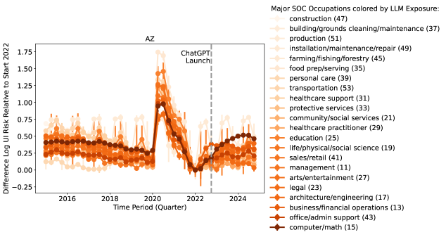
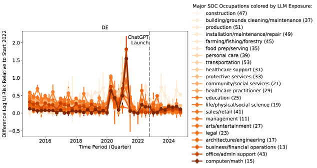
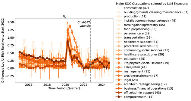
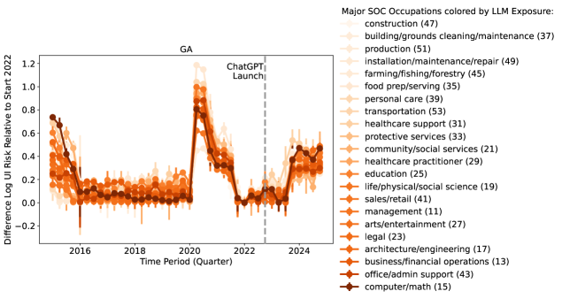
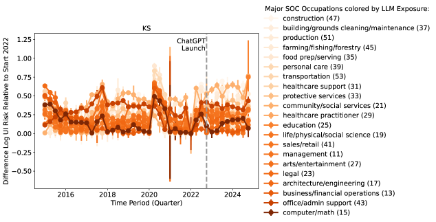
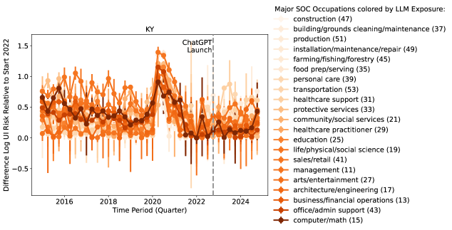
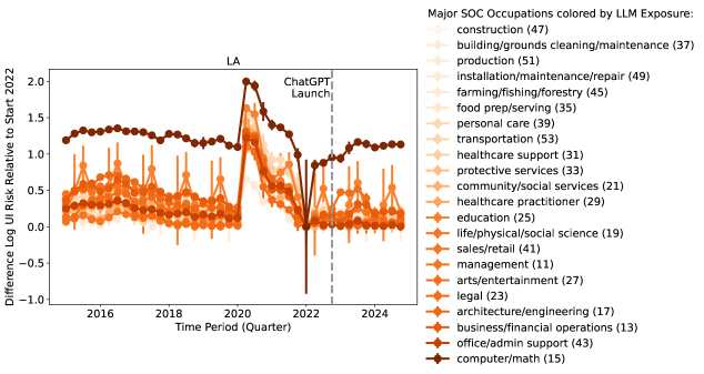
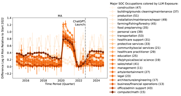
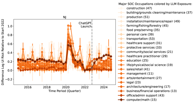
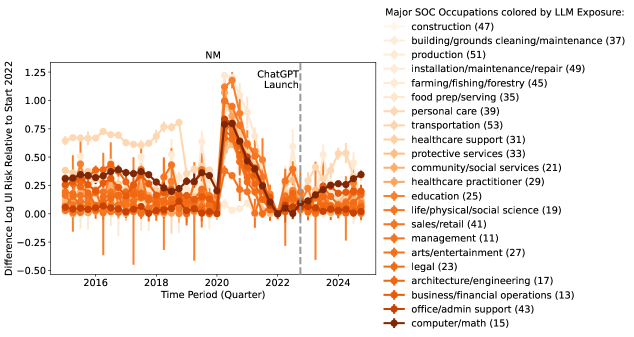
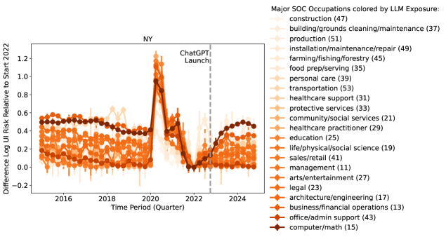
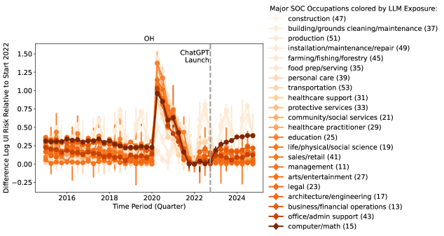
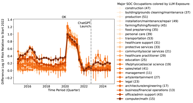
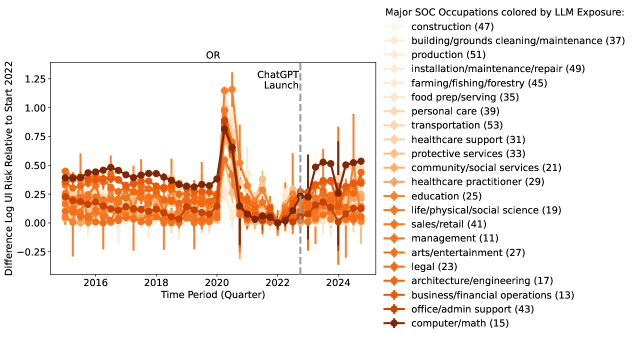
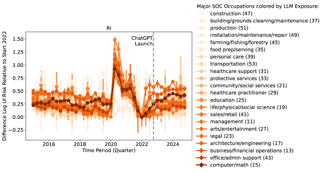
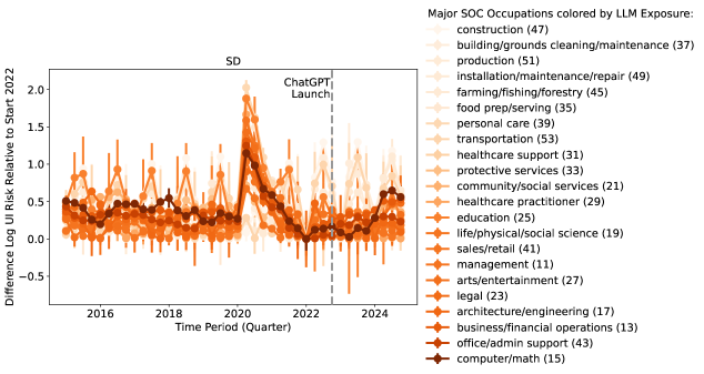
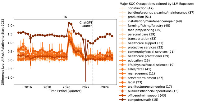
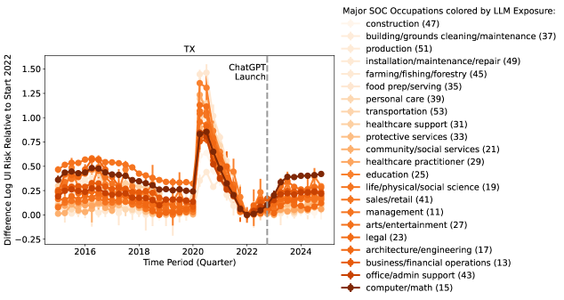
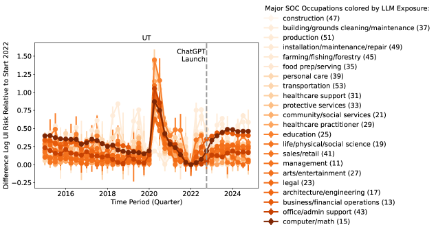
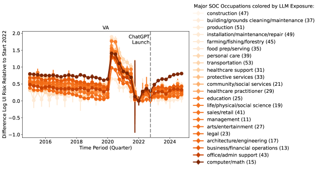
Disaggregating by major occupation group and normalizing to 2022Q1 (Fig.1C), computer and math occupations (SOC 15) exhibit the largest increase in unemployment risk during 2022–2024. This increase again begins prior to ChatGPT’s launch and flattens afterward. Most other occupation groups show little change around the launch date (Fig.S9). The only exception is office/administrative support occupations (SOC 43) which experience rising unemployment risk in the quarter after launch; however, this result disappears when omitting unemployment risk data from Connecticut (see Fig. S10). Overall, the timing is inconsistent with a deterioration that begins only after ChatGPT and suggests that pre-existing macroeconomic and sectoral forces contributed materially to the early-2022 rise in unemployment risk.

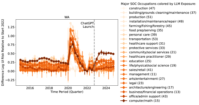
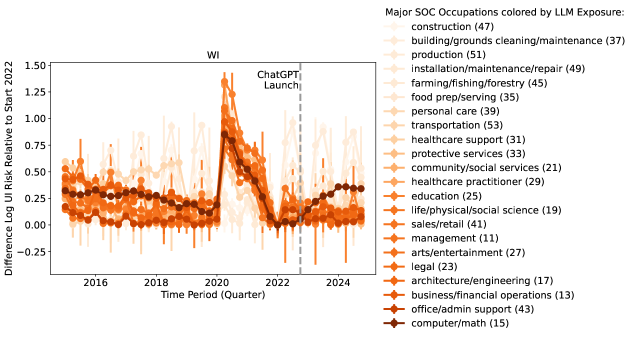
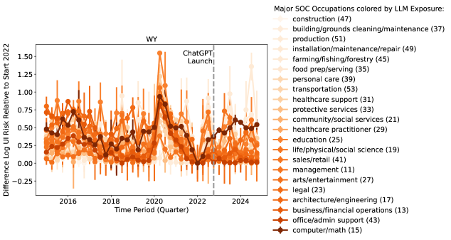
While these patterns hold nationally, a small number of states show post-launch increases in computer and math occupation unemployment risk (e.g., CA, WA, and AK; Figs. S15–S12). In these cases, timing alone cannot rule out a contribution from LLM diffusion. However, across states, post-launch unemployment risk remains comparable to pre-pandemic levels, suggesting limited movement in the longer-run equilibrium.

Labor market outcomes for recent college graduates

Unemployment risk separates unemployment dynamics by occupation but does not necessarily reflect career outcomes for subpopulations within a profession. For example, recent college graduates may not be eligible to claim unemployment benefits or may not have a most-recent occupation to include in their unemployment claim and would thus be absent from our analysis of unemployment risk. Meanwhile, anecdotes (e.g., from the CEO of Anthropic) and other recent studies (?) suggest that AI most impacts early-career workers competing for LLM exposed jobs. Thus, while unemployment risk reflects career outcomes in the workforce generally, it may not reflect the outcomes of workers who experience the bulk of AI’s impact.

We address this shortcoming with 10,584,980 individuals’ LinkedIn profiles provided by Revelio Labs. Each profile contains a worker’s education history, including degrees obtained, field of study, graduation year, and degree-granting university, as well as their career history, including job titles (i.e., mapped to six-digit SOC code), employers, job start dates, and job locations. Additionally, Revelio estimates the salary for each job using a proprietary machine learning model. This salary model uses position-specific information, such as job title, seniority level, company, and location, as well as user-specific information such as the number of years an individual has worked at the company, and is trained on salaries found in publicly-available visa application data, self-reported data, and job postings. We are not able to directly verify the estimated salaries against workers’ actual salaries. Therefore, we additionally consider college graduates’ months to first observed job within three years post-graduation; individuals without an observed job within the window are excluded. This measure requires only that individual’s update their profiles when they start a new job and again corresponds to friction in the job market if graduates spend more time job seeking.

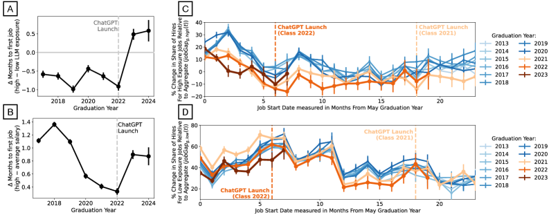
We examine job seeking for graduation cohorts while controlling for the monthly job opening rate in the state and month of their first job, fixed effects for the job’s state and sector, and fixed effects for the individuals’ education characteristics including terminal degree type, field of study, and degree-granting university (see Supplementary Materials Estimating College-Graduate Job Seeking Times for details). Additionally, we consider a job’s LLM exposure according to its six-digit SOC occupation code. In all years before the launch of ChatGPT, on average, graduates whose first job had high exposure spent less time job seeking than their peers (see Fig. 2A). However, graduates from 2023 and 2024 whose first job was exposed instead spent more time job seeking. These results suggest that the job market worsened for college graduates after ChatGPT’s launch.

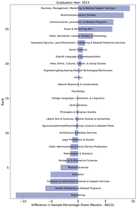
Occupations with the most LLM exposure are a subset of high-salary occupations (?). If the increase in job search times were specific to LLM-exposed occupations, an alternative salary-based comparison might produce a different result. Thus, we additionally examine the job delay of graduates whose first job was high salary compared to their peers earning average salaries from the same graduation cohort (see Fig. 2B). Consistent with our hypothesis, we observe a different trend for pre-pandemic graduates who spend more time job seeking. But the salary-based analysis moves in the same direction post-2022, suggesting a broader early-career tightening that is not specific to LLM-exposed workers.

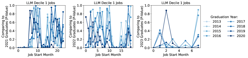
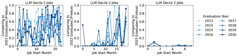
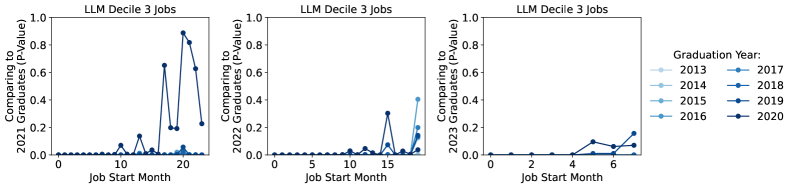
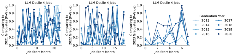
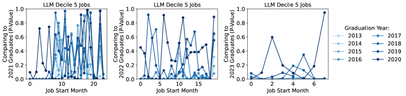
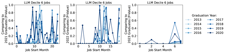
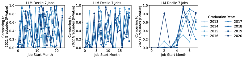
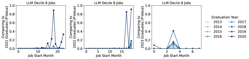
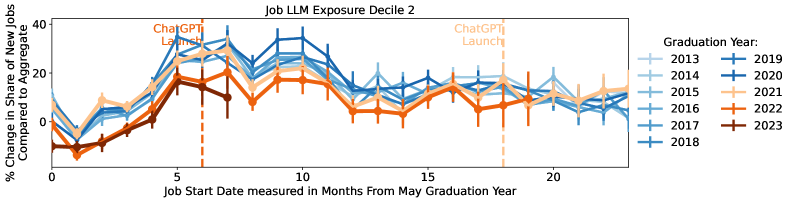
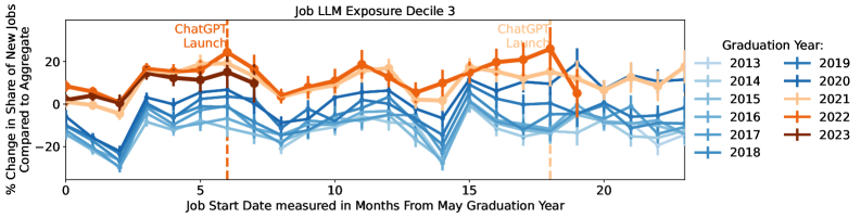
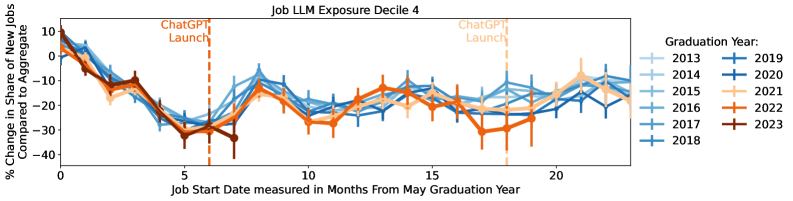
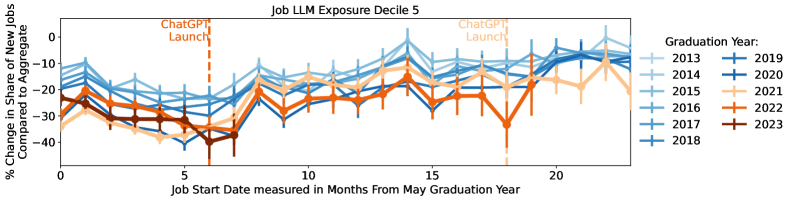
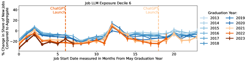
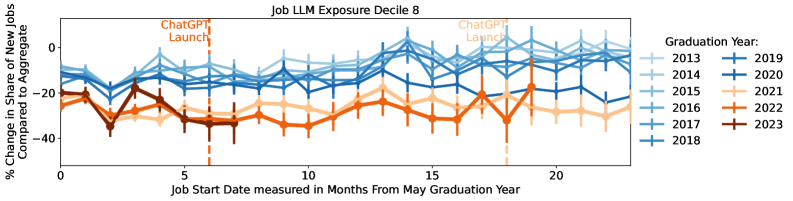
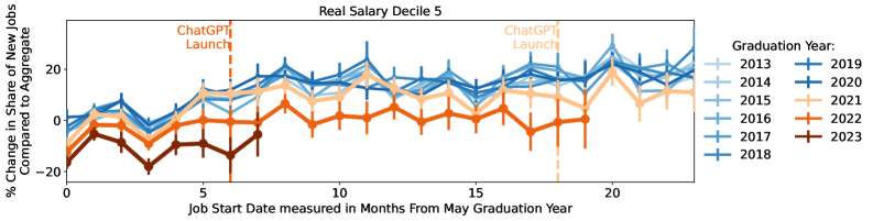
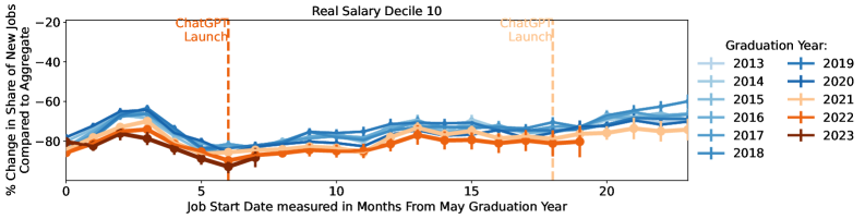
Do drops in job market performance correspond with the launch of ChatGPT? If so, then we should see graduates’ job market performance worsen only after the launch of ChatGPT. To measure the job seeking performance for graduation cohort $g$ based on their first jobs after terminal degree completion, we consider their over- or under-representation in newly started jobs of LLM exposure decile $llm$ relative to the overall job-start distribution. That is, we consider

jobGap_{g,llm}(t)=100\cdot\frac{p(g\mid t,\text{llm})-p(g\mid t)}{p(g\mid t)},

(1)

where $p(g\mid t,\text{llm})$ denotes the share of jobs with LLM exposure decile $llm$ started by graduates of class $g$ in month $t$ since May of their graduation year, and $p(g\mid t)$ denotes the corresponding share across all jobs (see Supplementary Materials Tracking Significant Difference in Graduation Cohort Job Gaps).

Across exposure deciles, graduation cohorts 2013 through 2020 each exhibit nearly identical $jobGap_{g,llm}$ trends in their first two years after graduation. For jobs started within each of the first four months after graduation, graduates secure a larger share of LLM-exposed jobs compared to the share of all jobs started. This difference in job finding rates gradually disappears around six months after May of the cohort’s graduation year.

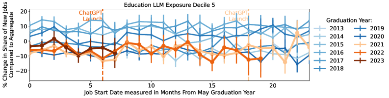
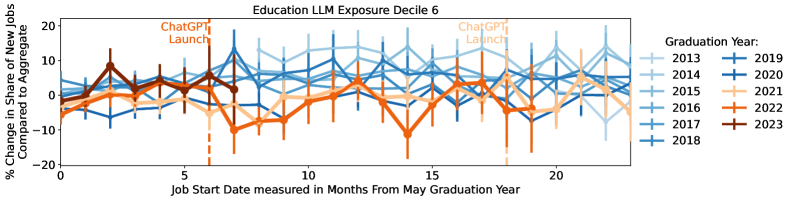
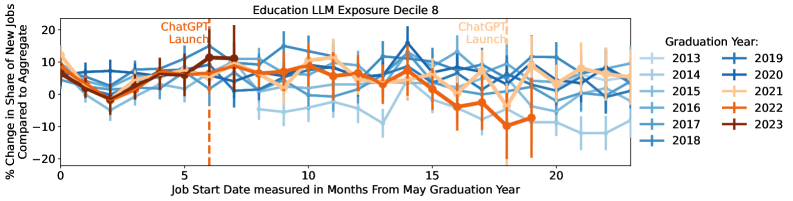
However, only graduate cohorts 2021, 2022, and 2023 would have experienced job markets with generative AI adoption within two years after degree completion. Compared to earlier cohorts, these graduates exhibit lower $jobGap_{g,llm}$ for the most LLM-exposed jobs (i.e., decile $llm=10$ . See Fig. 2C)) in their first few months in the labor market and then again at roughly one year after graduation. However, this low performance for 2021 and 2022 graduates starts months before the launch of ChatGPT (note 2023 graduates entered the workforce only after ChatGPT’s launch). As a robustness check, we additionally consider graduate cohorts’ $jobGap_{g,llm}$ trends for the least LLM exposed jobs (i.e., decile $llm=1$ ) and observe no period of significant difference (see Fig. 2D and Supplementary Materials Tracking Significant Difference in Graduation Cohort Job Gaps for statistical results). We provide similar analyses for all LLM-exposure deciles and, alternatively, for job salary deciles in the Supplementary Materials. We provide an alternative analysis of the share of jobs by LLM-exposure demonstrating consistent results in Supplementary Materials Monthly Graduation Cohort Job Shares.

Educational exposure to LLM-related skills

Regardless of AI’s culpability, the difficult job market exists. And students, educators, employers, and policymakers debate how higher education should change—both in terms of pedagogy (?) and workforce preparedness. For example, should students continue to learn skills that LLMs might automate, such as writing, coding, or information lookup? If LLMs primarily reduced the market value of LLM-adjacent skills, we might expect educational exposure to those skills to produce negative career outcomes after ChatGPT.

Table 1: Education exposure to LLM exposed tasks predicts better early-career outcomes after ChatGPT.

gpt=1

if job starts on or after December 2022.

edu

is the average of the number of LLM exposed tasks from matched syllabi (see SI for more details).

llm

is first-job occupation six-digit SOC code LLM exposure (?). Continuous predictors and dependent variables are centered and standardized (i.e., z-scores). All models include fixed effects for the state and two-digit NAICS code of the job as well as for the terminal degree type (e.g., bachelors or masters), graduation year, college field of study (i.e., two-digit CIP Code), and degree-granting university.

Number of Rows: 1,350,482
Dependent Variable:	Log Salary (Real 2015 $)		Months to First Job
Variable	Model 1	Model 2	Model 3	Model 4
Job Opening Rate	0.028^∗∗∗	0.029^∗∗∗	0.473^∗∗∗	0.472^∗∗∗
Major SOC Log Annual Wage (2020)	0.726^∗∗∗	0.644^∗∗∗	-0.044^∗∗∗	-0.034^∗∗∗
Post ChatGPT Indicator ( $gpt$ )	0.034^∗∗∗	0.031^∗∗∗	2.341^∗∗∗	2.344^∗∗∗
Education Exposure ( $edu$ )	0.000	-0.000	0.000^∗∗∗	0.000^∗∗∗
$edu\times gpt$	0.003^∗	0.001	-0.025^∗∗∗	-0.025^∗∗∗
LLM Exposure ( $llm$ )		0.564^∗∗∗		-0.096^∗∗∗
$gpt\times llm$		-0.064^∗∗∗		0.034^∗∗∗
$edu\times llm$		-0.019^∗∗∗		0.006^∗∗∗
$edu\times llm\times gpt$		0.012^∗∗∗		-0.009^∗∗∗
State FE	Yes	Yes	Yes	Yes
Sector FE	Yes	Yes	Yes	Yes
Terminal Degree Type FE	Yes	Yes	Yes	Yes
Graduation Year FE	Yes	Yes	Yes	Yes
College Major FE	Yes	Yes	Yes	Yes
University FE	Yes	Yes	Yes	Yes
$R^{2}$	0.426	0.433	0.374	0.374
adj. $R^{2}$	0.425	0.433	0.373	0.373
$p_{val}<0.1^{}$ , $p_{val}<0.01^{}$ , $p_{val}<0.001^{**}$

To investigate, we again turn to LinkedIn profiles and examine graduates’ first jobs within three years after degree completion. However, using profiles alone, our best proxy for education exposure to LLMs is workers’ self-reported field of study (i.e., college major) according to two-digit codes from the Classification of Instructional Programs (CIP) used by the National Center for Education Statistics. Thus, we augment worker profiles with 3 million U.S. higher education course syllabi (?) to assess each worker’s education LLM exposure $edu$ , defined as the number of LLM-exposed tasks (?) inferred from the syllabi associated with their graduation year, degree-granting university, and education field of study (see Materials and Methods).

After controlling for local labor-demand conditions (e.g., by state and sector (?)) and detailed education and job fixed effects, educational LLM exposure ( $edu$ ) is not meaningfully associated with first-job salary or time to first job for pre-ChatGPT job starts (Models 1 & 3). In contrast, for post-ChatGPT job starts, higher $edu$ predicts higher salaries and shorter job searches (positive $edu\times gpt$ for salary; negative $edu\times gpt$ for job seeking time). Jobs with higher occupation (i.e., six-digit SOC code) LLM exposure ( $llm$ ) are associated with weaker outcomes after ChatGPT (See Models 2 & 4 containing negative $gpt\times llm$ for salary; positive $gpt\times llm$ for months). However, the three-way interactions ( $edu\times llm\times gpt$ ) indicates that educational exposure partially offsets these post-ChatGPT penalties in more-exposed jobs after the widespread adoption of LLMs. The representativeness of each graduation cohort (e.g., by field of study) in the LinkedIn data is a limitation of this analysis; thus, we conduct additional analyses weighting worker profiles to mimic the graduates by field of study in the U.S. National Science Foundation’s National Survey of College Graduates and find consistent results (see Fig. S4-S8 and Table S4).

If LLMs were to blame for graduates’ poor job market performance, then we would expect to see that education exposure indicates redundant skills that do not add value when job seeking. Yet, our results suggest that teaching AI-exposed skills yields better outcomes for graduates after ChatGPT’s launch. These associations are difficult to reconcile with the view that LLM-relevant education became less valuable after ChatGPT. While not causal, they suggest that LLM-relevant preparation is at least compatible with better early-career outcomes in the post-ChatGPT period.

Discussion

Taken together, our results indicate that worsening labor-market outcomes in 2022–2024 for LLM-exposed workers and graduates were already underway prior to the mass-market emergence of LLM applications. Unemployment risk in highly exposed occupations rose beginning in early 2022—well before ChatGPT—and in most occupations and states we observe no discrete break coincident with its introduction. Early-career workers were affected disproportionately: graduates from the 2021–2023 cohorts entered highly exposed jobs at lower rates and experienced longer observed delays to their first job than earlier cohorts, with gaps opening, again, before late 2022. At the same time, LLM-relevant education remained valuable within this environment. Graduates whose programs exhibited greater pre-2020 curricular emphasis on LLM-exposed tasks earned higher first-job pay and reached their first jobs more quickly in the post-ChatGPT period, particularly when entering highly exposed occupations. Together, these patterns suggest that LLM diffusion occurred in a labor market already shaped by macroeconomic and sectoral forces, while LLM-complementary skills retained—and possibly increased—their labor-market value.

These findings have implications for research and policy. First, they caution against treating ChatGPT’s launch as a clean natural experiment for AI’s labor-market impact: designs that attribute post-2022 labor-market weakness primarily to LLMs risk confounding AI diffusion with concurrent macroeconomic shifts (possible examples include monetary policy, sectoral demand, and/or post-pandemic adjustment). Second, they suggest that higher education and workforce programs should not abandon skills often labeled “AI-exposed,” such as writing, coding, and information synthesis. Instead, curricula that teach these skills in LLM-complementary ways (e.g., by emphasizing verification, evaluation, and effective human–LLM collaboration) may improve graduates’ resilience in an uncertain labor market.

Our analyses rely on administrative unemployment insurance records, online career histories, task-based exposure measures, and syllabus-derived proxies for curricular content. Each source involves measurement error and selection. In particular, our educational exposure measure is derived from syllabi that predate 2020 and therefore captures baseline differences across programs rather than curricular responses to ChatGPT. Our time-to-first-job analyses exclude individuals whose first observed job begins more than three years after degree completion, which may understate delays among graduates facing the greatest barriers to entry. We do not identify the causal effect of LLMs on labor-market outcomes. Nonetheless, by triangulating across independent data sources, we document timing patterns that are difficult to reconcile with a sudden post-ChatGPT collapse in exposed occupations, shifting attention toward broader labor-market dynamics and toward expanding access to AI-complementary education. Future work combining direct measures of LLM adoption with linked worker–firm data will be critical for distinguishing displacement from productivity gains and for identifying which workers, regions, and institutions benefit—or fall behind—in the next phase of diffusion.

Acknowledgments

We are grateful for input from Daniel Rock, Esteban Moro, Martha Gimbel, Nathan Goldshlag, and Yong-Yeol Ahn.

Funding:

M. R. F. was funded by a grant from the Alfred P. Sloan Foundation, through a gift from Microsoft’s AI Economy Institute, and this work is supported by the University of Pittsburgh Center for Research Computing.

Author contributions:

All authors designed the research and drafted the manuscript. M.R.F. and A.J.S. gathered data and conducted the analysis.

Competing interests:

There are no competing interests to declare.

Data and materials availability:

Upon publication, all code will be publicly-available for download through a GitHub repository. Underlying worker profile data was provided by Revelio Labs and is not publicly available. However, data can be requested or purchased from Revelio Labs.

Supplementary materials

Materials and Methods
Supplementary Text
Figs. S1 to S105
Tables S1 to S4
References (17-0)

Supplementary Materials for
AI-exposed jobs deteriorated before ChatGPT

M.R. Frank^∗, A. Javadian Sabet, L. Simon, S.H. Bana, R. Yu
^∗Corresponding author. Email: mrfrank@pitt.edu

Materials and Methods

Unemployment Risk

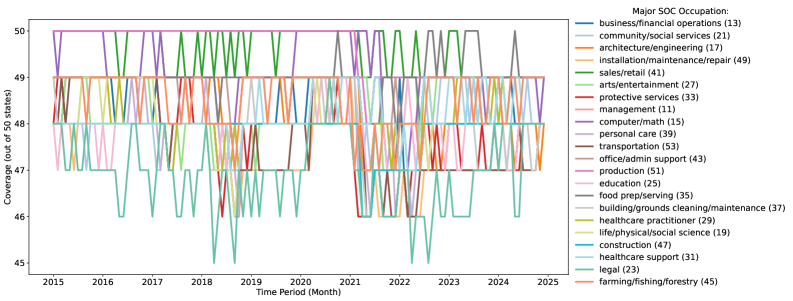
The ETA 203 (officially titled “Distribution of Characteristics of the Insured Unemployed”) is a monthly report submitted by state Unemployment Insurance (UI) agencies to the Employment & Training Administration (ETA) of the United States Department of Labor. The ETA 203 is a demographic & characteristics snapshot of continued UI claimants (specifically, the “insured unemployed”) across each state and for the nation as a whole. It is reported on a monthly basis, with data capturing the week including the 12th of the month which corresponds to the similarly-timed survey week for the Bureau of Labor Statistics (BLS) Current Population Survey (CPS). The data are submitted by states to the national office of ETA via the Office of Workforce Security. Coverage in the ETA 203 report for most states and occupations is good, but there are some exceptions; for example, California has no unemployment claimants for business/financial operations, management, education occupations between 2019 and 2025, but the data does contain counts for computer/math occupations (see Table S1). But, generally, coverage by occupation is typically good; in the worst case, there are four months where unemployment statistics for Legal occupations (Major SOC 23) was zero in five states (see Fig. S1); these statistics may in fact be accurate or, in the case of California for example, may represent a failure to align a state’s internal occupation classification system and the Standard Occupation Classification System (SOC). You can download the complete data set here: https://oui.doleta.gov/unemploy/csv/ar203.csv

ETA 203 Report compared to Census Current Populatiom Survey (CPS) Unemployment

The ETA 203 report (“Characteristics of the Insured Unemployed”) is an administrative unemployment insurance (UI) tabulation compiled from state UI systems that describes the demographic, industry, and occupation characteristics of the insured unemployed. In the ETA 203 framework, the insured unemployed are defined as regular state UI continued weeks claimed (intrastate plus interstate agent), excluding extended and other compensation programs (?). Importantly for comparisons to survey-based unemployment statistics, ETA guidance aligns the ETA 203 “survey week” to the Current Population Survey (CPS) reference week (typically the week containing the 12th of the month), operationalized through continued weeks claimed filed during the week containing the 19th, and explicitly notes that ETA 203 characteristics can be compared to characteristic figures for the CPS total unemployed (?, ?, ?). By contrast, CPS unemployment is a population-representative household survey construct rather than a program-based count, and cannot be inferred from UI rolls because many unemployed individuals are ineligible for UI, do not apply, or exhaust benefits (?).

Empirical benchmarks underscore both the value and the limitations of ETA 203–CPS comparisons. Cortes and Forsythe compare CPS-predicted UI recipients to actual UI recipients reported to the U.S. Department of Labor (DOL) via the ETA 203 system during April 2020–February 2021, emphasizing that the DOL administrative compilation aggregates state reports of varying quality and exhibits substantial missingness for some variables (e.g., race and occupation) (?). Their comparisons show close agreement for some characteristics (e.g., female and Hispanic shares) alongside larger discrepancies for others (e.g., Black and older-age shares), which they interpret as potentially reflecting CPS classification issues in certain contexts and/or reporting differences across sources (?). Taken together, these resources suggest that ETA 203–CPS comparisons are most defensible when framed explicitly as contrasts between insured unemployment (receipt/claims-based) and total unemployment (labor-force-status-based), with careful attention to timing alignment, program scope (regular UI only), and item-specific data quality in administrative tabulations (?, ?, ?).

Calculating Unemployment Risk

Combined with employment statistics, we calculate an occupation’s unemployment risk according to

p(unemp|soc,s,t)=\frac{4\cdot n(unemp|soc,s,t)}{4\cdot n(unemp|soc,s,t)+n(emp|soc,s,t)}

(S1)

where $emp$ indicates a worker is employed, $unemp$ indicates a worker is unemployed, $soc$ denotes an occupation’s two-digit Standard Occupation Classification (SOC) code, $s$ denotes a state, $t$ denotes a time period (i.e., year and month), and $n$ captures the number of employed or unemployed workers by occupation, state, and time period. $n(unemp|soc,s,t)$ comes from the detailed unemployment data while $n(emp|soc,s,t)$ comes from annual BLS OEWS. We multiply $n(unemp|soc,s,t)$ by $4$ to roughly scale from one week of data to one month under the assumption that the week including the 12th of the month is representative of the whole month. Employment by occupation within a state $n(emp|soc,s,t)$ varies annually and so we use it here missing monthly variation. Given a state and time, $p(unemp|soc,s,t)$ is the probability that a worker with occupation $soc$ claims continuing unemployment benefits. Unemployment risk varies by occupation (e.g., construction workers versus transportation workers) while controlling for states’ total labor market size and occupations’ local employment share (e.g., more retail workers may receive unemployment benefits in a state where retail workers are a larger share of employment).

Many studies focus on an occupation’s change in employment following a technological disruption, so one might assume that an occupation’s rising employment would directly correspond to falling unemployment risk. Similarly, a more typical analysis of a state’s total unemployment rate may sufficiently explain variation in unemployment risk as being largely driven by systemic economic factors rather than factors varying by occupation. Using Bayes’ Theorem, we can relate an occupation’s unemployment risk to its local employment share and the state’s total unemployment rate according to

p(unemp|soc,s,t)=\frac{p(soc|unemp,s,t)\cdot p(unemp|s,t)}{p(soc|emp\cup unemp,s,t)}

(S2)

where $p(unemp|s,t)$ is the total unemployment rate from BLS LAUS and $p(soc|emp\cup unemp,s,t)$ is the share of the local labor force associated with $soc$ . However, as Figure 1 in (?) shows, an occupation’s employment share over time within a state has no consistent empirical relationship with the occupation’s unemployment risk. And, an occupation-state pair’s unemployment risk co-varies with the state’s total unemployment rate over time but not always.

In Figure 1A, we estimate differences in unemployment risk for low- and high-exposure occupations using the interaction terms $\beta_{t}$ from the following ordinary least squares regression model:

\log\left(p(unemp|soc,s,t)\right)\sim\sum_{t\in T}\alpha_{t}\cdot I_{t}+\beta_{t}\cdot I_{t}\cdot llm_{soc}

(S3)

where $T$ indexes over quarters each year, $llm(soc)\in[0,1]$ is the average AI-exposure (?) of the major occupation group $soc\in SOC$ , and $I_{t}$ is an indicator variable for time $t$ . As a result, $100\cdot(e^{\beta_{t}}-1)$ describes the percentage change in unemployment risk in a given quarter as $llm_{soc}$ varies from $llm_{soc}=0$ to $llm_{soc}=1$ .

Table S1: Missing data from the ETA 203 report. For each major occupation group and state, the number of months with zero continuing unemployment claimants between January 2020 through December 2024 (i.e., 60 is the maximum). States with no missing data are omitted.

Major Occupation Group	State
	DE	CT	CA	NE	KY	NH	VT	AK	KS	SD
sales/retail (41)	3	0	0	0	0	0	33	0	0	0
protective services (33)	5	28	60	0	17	0	46	0	0	0
education (25)	5	7	60	0	10	0	43	0	0	0
office/admin support (43)	0	0	59	0	0	0	45	0	0	0
life/physical/social science (19)	0	23	60	0	1	0	46	0	0	0
production (51)	4	0	0	0	0	0	44	0	0	0
computer/math (15)	1	10	0	3	3	0	39	0	0	0
healthcare practitioner (29)	3	30	60	0	0	0	27	0	0	0
construction (47)	3	30	60	0	0	0	45	0	0	0
healthcare support (31)	2	15	60	0	1	0	19	0	0	0
transportation (53)	2	6	60	0	1	45	44	0	0	0
management (11)	0	30	60	0	0	0	45	0	0	0
architecture/engineering (17)	3	0	60	0	4	0	45	0	0	0
business/financial operations (13)	3	10	60	0	0	0	34	0	0	0
installation/maintenance/repair (49)	3	13	60	0	0	0	45	0	58	0
community/social services (21)	2	25	60	0	9	0	15	0	0	0
arts/entertainment (27)	1	10	60	0	0	0	30	0	0	0
personal care (39)	1	22	60	0	3	0	46	0	0	0
legal (23)	3	29	60	0	33	0	37	17	0	2
building/grounds cleaning/maintenance (37)	4	18	60	0	7	0	45	0	0	0
farming/fishing/forestry (45)	13	30	1	0	4	0	46	0	0	0
food prep/serving (35)	3	29	0	0	0	0	27	0	0	0

Estimating College-Graduate Job Seeking Times

We first filter to individuals in the Revelio Labs worker profile data who “graduated” (i.e., completed their terminal degree) in 2017 through 2024. We then filter each individual’s work history to their first job after degree completion restricting to within three years of degree completion. When an exact graduation is not provided, we assume a May graduation in the year of the individual’s terminal degree completion. Each job has an salary estimated by Revelio Labs, which we convert to real 2015 dollars, and an AI-exposure score (?). Individual $i$ ’s $jobDelay_{i}$ is the number of months between terminal degree completion and start date of each graduate’s first post-graduation job.

We study early-career outcomes for college graduates by graduation cohort using an event study focused around the launch of ChatGPT in November 2022. We estimate an ordinary least-squares regression model of the form

	$\displaystyle jobDelay_{i}$	$\displaystyle\sim\sum_{g\in G}\left(\beta_{g}\cdot I_{g}+\beta_{g,llm}\cdot I_{g}\cdot llm_{i}\right)+\beta_{openings}\cdot jobOpeningRate_{i}$
		$\displaystyle+\sum_{s\in State}\beta_{s}\cdot I_{s}+\sum_{n\in NAICS2}\beta_{n}\cdot I_{n}+\sum_{fos\in FieldOfStudy}\beta_{fos}\cdot I_{fos}$
		$\displaystyle+\sum_{d\in Degrees}\beta_{d}\cdot I_{d}+\sum_{u\in Universities}\beta_{U}\cdot I_{u}$

where $\beta$ represent regression coefficients, $I_{g}$ is an indicator variable for the year of terminal degree completion, $llm_{i}$ is the LLM exposure of the first job after graduation (i.e., according to six-digit SOC code), $jobOpeningRate_{i}$ is the job opening rate in the state and month of the job according to BLS JOLTS, $I_{s}$ is an indicator variable for the state of the job, $I_{n}$ is an indicator variable for the sector of the job (i.e., two-digit NAICS code), $I_{fos}$ is the field of study of the individual’s terminal degree (i.e., two-digit codes from the Classification of Instructional Programs (CIP) used by the National Center for Education Statistics), $I_{d}$ is an indicator variable for the type of terminals degree (i.e., GED, associates, bachelors, masters, MBA, or doctoral), and $I_{u}$ is an indicator variable for the university or college from which the individual earned their terminal degree (e.g., University of Pittsburgh). Each regression contains 2,665,306 individuals (i.e., rows of data). We conduct an additional but similar regression swapping LLM exposure ( $llm_{i}$ ) for the estimated salary of the first job ( $salary_{i}$ ).

Workers’ Education Exposure to AI

We augment worker profiles with a dataset (?) of 3 million US higher education course syllabi from the Open Syllabus Project. For each syllabus $s$ , we compute a vector $\vec{t}_{s}\in\mathbb{R}^{|T|}$ of semantic similarities between the learning objectives of the course and each O*NET task $t\in T$ . Let $\vec{e}\in[0,1]^{|T|}$ be the task–level exposure vector (?) under GPT-4, Rubric 1 $\beta$ , containing a 1 if a task is exposed to automation from LLMs. We define the syllabus–level education exposure as the dot product $edu_{s}\;=\;\vec{t}_{s}\cdot\vec{e}.$ Finally, given a single worker profile, we estimate the worker’s education exposure as the average $edu_{s}$ for syllabi from the profile’s education field of study, degree-granting institution, and the four years leading up to and including their graduation year.

This approach has several limitations. First, the syllabus data is a subset of all US higher education. Second, the most recent syllabi available are for courses offered in 2017. For workers who graduated after 2017, we default to the relevant syllabi from years 2014-2017 and we consider their education exposure in the context of status quo educational activity from before the COVID pandemic and before generative AI. Despite these limitations, to the best of our knowledge, there is no better data for estimating the difference in teaching across fields of study, educational institutions, and graduation years (see Table S2 for average $edu_{s}$ across fields of study and Table S3 for the most and least exposed universities.)

Table S2: Average

edu_{s}

by field of study (two-digit CIP code) rounded to the nearest integer. Fields are ordered from highest to lowest average

edu_{s}

CIP Code	CIP Title	Avg. $edu_{s}$	Syllabus Count
44	PUBLIC ADMINISTRATION AND SOCIAL SERVICE PROFESSIONS.	1996	22,171
52	BUSINESS, MANAGEMENT, MARKETING, AND RELATED SUPPORT SERVICES.	1970	229,512
41	SCIENCE TECHNOLOGIES/TECHNICIANS.	1899	5,970
51	HEALTH PROFESSIONS AND RELATED PROGRAMS.	1870	218,642
47	MECHANIC AND REPAIR TECHNOLOGIES/TECHNICIANS.	1862	25,364
19	FAMILY AND CONSUMER SCIENCES/HUMAN SCIENCES.	1849	54,320
46	CONSTRUCTION TRADES.	1843	26,303
04	ARCHITECTURE AND RELATED SERVICES.	1840	17,779
12	CULINARY, ENTERTAINMENT, AND PERSONAL SERVICES.	1838	16,256
29	MILITARY TECHNOLOGIES AND APPLIED SCIENCES.	1837	18,290
43	HOMELAND SECURITY, LAW ENFORCEMENT, FIREFIGHTING AND RELATED PROTECTIVE SERVICES.	1832	100,072
31	PARKS, RECREATION, LEISURE, FITNESS, AND KINESIOLOGY.	1832	79,198
09	COMMUNICATION, JOURNALISM, AND RELATED PROGRAMS.	1829	68,891
13	EDUCATION.	1813	391,918
15	ENGINEERING/ENGINEERING-RELATED TECHNOLOGIES/TECHNICIANS.	1812	58,488
25	LIBRARY SCIENCE.	1807	7,276
10	COMMUNICATIONS TECHNOLOGIES/TECHNICIANS AND SUPPORT SERVICES.	1795	34,791
42	PSYCHOLOGY.	1773	81,603
01	AGRICULTURAL/ANIMAL/PLANT/VETERINARY SCIENCE AND RELATED FIELDS.	1761	28,312
49	TRANSPORTATION AND MATERIALS MOVING.	1758	23,422
11	COMPUTER AND INFORMATION SCIENCES AND SUPPORT SERVICES.	1754	126,678
48	PRECISION PRODUCTION.	1741	4,244
03	NATURAL RESOURCES AND CONSERVATION.	1733	8,924
14	ENGINEERING.	1707	34,159
26	BIOLOGICAL AND BIOMEDICAL SCIENCES.	1693	142,118
50	VISUAL AND PERFORMING ARTS.	1687	185,898
24	LIBERAL ARTS AND SCIENCES, GENERAL STUDIES AND HUMANITIES.	1679	8,667
23	ENGLISH LANGUAGE AND LITERATURE/LETTERS.	1678	186,199
22	LEGAL PROFESSIONS AND STUDIES.	1660	44,008
39	THEOLOGY AND RELIGIOUS VOCATIONS.	1659	31,960
45	SOCIAL SCIENCES.	1642	133,580
30	MULTI/INTERDISCIPLINARY STUDIES.	1632	70,527
40	PHYSICAL SCIENCES.	1627	133,964
27	MATHEMATICS AND STATISTICS.	1620	204,848
38	PHILOSOPHY AND RELIGIOUS STUDIES.	1526	40,161
54	HISTORY.	1523	51,186
05	AREA, ETHNIC, CULTURAL, GENDER, AND GROUP STUDIES.	1510	72,981
16	FOREIGN LANGUAGES, LITERATURES, AND LINGUISTICS.	1497	85,926

Table S3: The ten universities with highest and lowest average

edu_{s}

rounded to the nearest integer.

University Name	Avg. $edu_{s}$	Syllabus Count
New Mexico Junior College	2355	16,633
Modesto Junior College	2159	10,779
Park University	2032	27,096
Fresno City College	2017	24,786
Kentucky Community and Technical College System	2015	10,244
Rowan-Cabarrus Community College	1997	33,403
Hartnell College	1987	16,516
South Texas College	1977	11,998
Clark State Community College	1974	46,094
Santa Rosa Junior College	1959	35,613
$\vdots$	$\vdots$	$\vdots$
Loyola University New Orleans	1636	15,398
Midwestern State University	1622	25,202
Minnesota State Colleges and Universities System	1592	22,869
Alamo Colleges	1588	159,995
University of Alabama, Tuscaloosa	1560	53,368
Galveston College	1476	18,908
Wilkes University	1338	10,008
University of Michigan–Ann Arbor	1253	23,798
University of California, Irvine	1252	11,834
Princeton University	1223	11,667

Weighting Revelio Graduates to Match NCSG Survey Graduates

The National Survey of College Graduates (NSCG) is a biennial survey sponsored by the U.S. National Science Foundation’s National Center for Science and Engineering Statistics (NCSES) and conducted by the U.S. Census Bureau. The survey provides nationally oriented data on the characteristics of U.S. college graduates, with particular emphasis on the science and engineering workforce. In the 2023 cycle, the target population is non-institutionalized residents of the United States or Puerto Rico who have earned at least a bachelor’s degree and are younger than 76 as of the survey reference date. The NSCG is drawn from the American Community Survey (ACS) sampling frame and uses a four-panel rotating panel design in which each new panel completes a baseline interview followed by up to three biennial follow-ups before rotating out. Data are collected via a tri-modal approach (web, mail, and CATI), and the public-use files include final survey weights designed to support unbiased population inference under the complex design; for the 2023 cycle, NCSES reports a weighted response rate of 61% and notes that sampling errors are computed via successive difference replication.

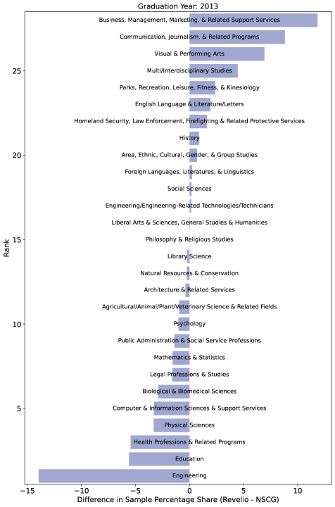
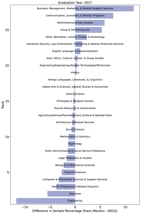
In studies using LinkedIn worker profiles—which are typically a non-probability sample whose composition can differ systematically from the population of college graduates—the NSCG can serve as an external benchmark to re-weight analyses toward population-representative estimates for outcomes observable on LinkedIn. Concretely, we compare the distribution of graduates by college field of study in the Revelio/LinkedIn data to the distribution in the corresponding graduation year in NSCG (see Fig. S4-S8). Typically, compared to the NSCG, the Revelio worker profile data over samples Business and Communications majors and under samples Engineering and Education majors.

We can then weight our sample of LinkedIn profiles for the biennial graduation years in the NSCG so the distribution college fields of study are identical and repeat our analysis of earnings and job seeking time in graduates first job after degree completion (compare main text Table 1 to the weighted analysis on a subset of graduation cohorts in Table S4). In the weighted analysis, key results from the main regression remain unchanged or are perhaps stronger. Education exposure ( $edu$ ) has almost no relationship with salaries or job seeking times before the launch of ChatGPT, but becomes more predictive afterwards. In particular, the three-way interaction ( $edu\times llm\times gpt$ ) continues to indicate the added value of educational exposure for graduates whose first job after degree completion is LLM-exposed after ChatGPT.

Table S4: Similar to Table 1 where we restrict the user sample to Bachelors degree recipients from graduation cohorts from 2015, 2019, 2021, and 2023 to match the NSCG survey and run OLS regression weighting individuals’ by their major to match graduation distributions over field of study according to NSCG survey.

gpt=1

if job starts on or after December 2022.

edu

is the average of the number of LLM exposed tasks from matched syllabi (see SI for more details).

llm

is first-job occupation six-digit SOC code LLM exposure (?). Continuous predictors and dependent variables are centered and standardized (i.e., z-scores). All models include fixed effects for the state and two-digit NAICS code of the job as well as for graduation year, college field of study (i.e., two-digit CIP Code), and degree-granting university. We do not include a terminal degree type fixed effect here because the sample is restricted to workers whose terminal degree is a bachelors degree.

Number of Rows: 1,005,479
Dependent Variable:	Log Salary (Real 2015 $)		Months to First Job
Variable	Model 1	Model 2	Model 3	Model 4
Job Opening Rate	0.033^∗∗∗	0.037^∗∗∗	0.405^∗∗∗	0.404^∗∗∗
Major SOC Log Annual Wage (2020)	0.906^∗∗∗	0.745^∗∗∗	-0.087^∗∗∗	-0.050^∗∗∗
Post ChatGPT Indicator ( $gpt$ )	-0.012	0.020^∗	3.280^∗∗∗	3.270^∗∗∗
Education Exposure ( $edu$ )	-0.000^∗∗∗	-0.000^∗∗∗	0.000^∗∗∗	0.000^∗∗∗
$edu\times gpt$	0.020^∗∗∗	0.006^∗	-0.020^∗∗∗	-0.017^∗∗∗
LLM Exposure ( $llm$ )		0.887^∗∗∗		-0.238^∗∗∗
$gpt\times llm$		-0.078^∗∗∗		0.052^∗∗∗
$edu\times llm$		-0.037^∗∗∗		0.006^∗∗∗
$edu\times llm\times gpt$		0.026^∗∗∗		-0.016^∗∗∗
State FE	Yes	Yes	Yes	Yes
Sector FE	Yes	Yes	Yes	Yes
Graduation Year FE	Yes	Yes	Yes	Yes
College Major FE	Yes	Yes	Yes	Yes
$R^{2}$	0.360	0.369	0.165	0.165
adj. $R^{2}$	0.360	0.369	0.165	0.165
$p_{val}<0.1^{}$ , $p_{val}<0.01^{}$ , $p_{val}<0.001^{**}$

Supplementary Text

Unemployment Risk by Major Occupation Group

Unemployment risk by State and Major Occupation Group

Tracking Significant Difference in Graduation Cohort Job Gaps

To determine whether the relative change in job-start shares for LLM-exposed jobs differs significantly across graduation cohorts, we construct a month-by-month test based on a Delta-method approximation of the sampling variability of the statistic of interest. For a given graduation cohort $g$ in month $t$ , let $p(g\mid t,\text{llm})$ denote the share of LLM-exposed jobs started by graduates of class $g$ , and let $p(g\mid t)$ denote the corresponding share across all jobs. The quantity of interest is the proportional difference

jobGap_{g,llm}(t)=\frac{p(g\mid t,\text{llm})-p(g\mid t)}{p(g\mid t)},

which measures how over- or under-represented graduates of class $g$ are in newly started LLM-exposed jobs relative to the overall job-start distribution. Because $p(g\mid t,\text{llm})$ and $p(g\mid t)$ are estimated from finite samples—specifically, binomial proportions based on the counts of LLM-exposed jobs and all jobs, respectively—we approximate their joint sampling distribution using a multivariate normal form and apply the Delta method to obtain an analytic expression for $\operatorname{Var}(jobGap_{g,llm}(t))$ . Under an independence assumption between the two estimates, this variance reduces to a closed-form expression involving the binomial variances of $\hat{p}(g\mid t,\text{llm})$ and $\hat{p}(g\mid t)$ .

Having obtained $\widehat{\operatorname{Var}}(jobGap_{g,llm}(t))$ for each graduation cohort and month, we test whether two cohorts $g_{1}$ and $g_{2}$ differ significantly by evaluating the null hypothesis $H_{0}:jobGap_{g_{1},llm}(t)=jobGap_{g_{2},llm}(t)$ for each month $t$ . The test statistic is a standard $z$ -score,

z_{g_{1},g_{2},llm}(t)=\frac{jobGap_{g_{1},llm}(t)-jobGap_{g_{2},llm}(t)}{\sqrt{\widehat{\operatorname{Var}}(jobGap_{g_{1},llm}(t))+\widehat{\operatorname{Var}}(jobGap_{g_{2},llm}(t))}},

which compares the estimated difference in representation against its sampling uncertainty. The resulting two-sided $p$ -value identifies the months in which the two graduation cohorts differ significantly in how strongly they are represented among new LLM-exposed job starts. This approach provides a transparent, nonparametric month-by-month comparison that directly targets the statistic used in descriptive figures while maintaining principled statistical inference through variance estimation and standard error propagation.

Graduation Cohort Job Gaps by Occupations’ AI-Exposure Decile

Graduation Cohort Job Gaps by Occupations’ Salary Decile

Graduation Cohort Job Gaps by Education Exposure Decile

Monthly Graduation Cohort Job Shares

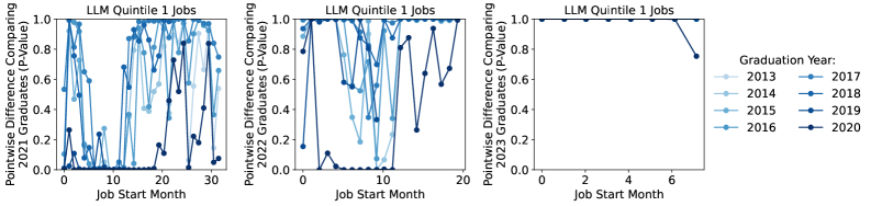
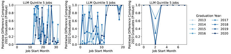
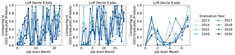
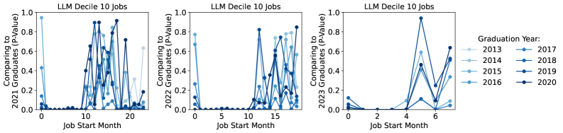
The pointwise difference test is a simple and widely used method for determining whether two time series of probabilities differ at specific points in time. We use it here as a robustness check to compare the job market performance by graduation cohort based on jobs started each month since May of their graduation year (i.e., similar to Fig. 2). For a given graduation cohort $g$ , we create a time series $p(g|t,llm)$ representing the share of jobs started in a given month $t$ (i.e., number of months since May graduation year) with LLM exposure (?) quintile $llm$ . That is, $p(g|t,llm)=x_{g,t,llm}/n_{t_{g},llm}$ where $x_{g,t,llm}$ is the number of jobs started in month $t$ within LLM exposure quintile $llm$ by members of graduation cohort $g$ and $n_{t_{g},llm}$ is the total number of jobs within LLM exposure quintile $llm$ started in month $t_{g}$ by anybody. Here, we index the month $t_{g}$ with graduation cohort $g$ because the month $t_{g}$ is relative to the graduation cohort $g$ ; that is, $t_{2016}=2$ is June 2016, two months from May of the graduation year 2016, while $t_{2022}=2$ is June 2022. We construct a time series in this way for each graduation cohort from 2013 through 2023.

At each month from May graduation year, we compare the time series for each pre-ChatGPT graduation cohort (i.e., 2013 through 2020) to graduation cohorts that experienced ChatGPT’s launch while they were new to the labor market (i.e., 2021, 2022, 2023). For each pair of time series $p(g_{1}|t,llm)$ and $p(g_{2}|t,llm)$ , we calculate the pointwise difference statistic according to

z_{g_{1},g_{2},t,llm}=\frac{p(g_{1}|t,llm)-p(g_{2}|t,llm)}{\sqrt{p_{t,llm}(1-p_{t,llm})\left(\frac{1}{n_{t_{g1},llm}}+\frac{1}{n_{t_{g_{2}},llm}}\right)}}

(S4)

where

p_{t,llm}=\frac{x_{g_{1},t,llm}+x_{g_{2},t,llm}}{n_{t_{g_{1}},llm}+n_{t_{g_{2}},llm}}

(S5)

is the pooled proportion. $z_{g_{1},g_{2},t,llm}$ measures how many standard errors apart the two observed probabilities are. A value of $z_{g_{1},g_{2},t,llm}$ near zero indicates that the difference between the two estimates is small relative to sampling noise, while large positive or negative values indicate stronger evidence against the null.

Interpreting the statistic proceeds in the same way as any standard normal $z$ -test: one computes a one-sided $p$ -value to test if $p(g_{2}|t,llm)$ (here, $g_{2}\in\{2021,2022,2023\}$ ) is statistically significantly lower than $p(g_{1}|t,llm)$ according to $p_{value}=1-\Phi(|z_{t}|)$ , where $\Phi(\cdot)$ is the standard normal cumulative distribution function. If this $p$ -value falls below a predetermined significance level (e.g., $0.05$ ), then the difference at time $t$ is deemed statistically significant. Because the test is conducted independently at each time point, we plot the sequence of $p_{value}$ values to visualize when the series diverge (see Fig. S101 through Fig. S105). In Figure S105, we examine graduate cohort performance in the occupations with the greatest AI-exposure and find that graduation cohorts 2021 and 2022 are often significantly under-performing compared to earlier graduation cohorts in their first year post-graduation. As a kind of placebo test, Figure S101 compares performance in the jobs with least AI-exposure. This analysis serves as robustness check on our main analysis in Figure 2. But this alternative approach does not control for the differences in labor market conditions in month $t_{g_{1}}$ and $t_{g_{2}}$ which are in fact different points in time.