A Wachspress-based transfinite formulation for exactly enforcing Dirichlet boundary conditions on convex polygonal domains in physics-informed neural networks

Abstract

In this paper, we present a Wachspress-based transfinite formulation on convex polygonal domains for exact enforcement of Dirichlet boundary conditions in physics-informed neural networks. This approach leverages prior advances in geometric design such as blending functions and transfinite interpolation over convex domains. For prescribed Dirichlet boundary function $\mathcal{B}$, the transfinite interpolant of $\mathcal{B}$, $g:\bar{P}\to C^{0}(\bar{P})$, lifts functions from the boundary of a two-dimensional polygonal domain to its interior. The transfinite trial function is expressed as the difference between the neural network’s output and the extension of its boundary restriction into the interior of the domain, with $g$ added to it. This ensures kinematic admissibility of the trial function in the deep Ritz method. Wachspress coordinates for an $n$-gon are used in the transfinite formula, which generalizes bilinear Coons transfinite interpolation on rectangles to convex polygons. Since Wachspress coordinates are smooth, the neural network trial function has a bounded Laplacian, thereby overcoming a limitation in a previous contribution where approximate distance functions were used to exactly enforce Dirichlet boundary conditions. For a point $\bm{x}\in\bar{P}$, Wachspress coordinates $\bm{\lambda}:\bar{P}\to[0,1]^{n}$ serve as a geometric feature map for the neural network: $\bm{\lambda}$ encodes the boundary edges of the polygonal domain. This offers a framework for solving problems on parametrized convex geometries using neural networks. The accuracy of physics-informed neural networks is successfully assessed on forward problems (linear and nonlinear), an inverse heat conduction problem, and a parametrized geometric Poisson boundary-value problem.

1 Introduction

As a computational paradigm, physics-informed neural networks (PINNs) [1] provide new pathways to solve forward, inverse and parametric design problems. In addition, they not only allow the ability to incorporate data and physics into the solution procedure, but also to solve for nonlinear differential operators [2, 3, 4]. For the forward problem, the simplest view of PINNs is as a collocation-based meshfree computational method on the strong form [5, 6]. A neural network approximation is formed via composition of nonlinear functions, with unknown parameters residing in the contribution of each neuron, which renders the trial function (ansatz) to not be known a priori. To solve a partial differential equation (PDE) over a bounded domain, a set of collocation points is chosen in its interior and another set of collocation points on the boundary (soft imposition of boundary conditions). The objective (loss) function is written as the sum of the mean squared error of the PDE in the interior of the domain (PDE loss) and the mean squared error associated with the prescribed boundary conditions (boundary loss). In addition, if the solution is also provided at specific collocation points in the interior of the domain, then the mean squared error associated with this data (data loss) is also included in the loss function. The resulting loss function is minimized via model training to determine the optimal set of parameters. An overview of recent advances in scientific machine learning is presented in [7].

The minimization of the loss function is a highly nonlinear, nonconvex optimization problem. It has been broadly appreciated that the presence of PDE loss and boundary loss terms in the objective function adversely affects model training [8, 9, 10, 11], and the know-how that this issue is related to finding pareto-optimal solutions in multiobjective optimization [12]. For boundary-value problems, satisfying boundary conditions exactly (hard imposition) through the neural network ansatz is desirable, as it simplifies the optimization landscape by reducing the objective to a single PDE loss term. The main contribution of this paper is a novel construction of a transfinite neural network trial function that exactly enforces Dirichlet boundary conditions on convex polygonal domains. This formulation adopts Wachspress coordinates [13] as blending functions in a transfinite interpolant on convex domains [14]. The proposed approach ensures that the trial function has a bounded Laplacian, thereby overcoming a key limitation from previous work [15] in which the Laplacian of the trial function was unbounded at the vertices of a polygonal domain. The detailed contributions in this work with key features of the new formulation are described in Section 1.2.

1.1 Related work

Early attempts to strongly enforce Dirichlet boundary conditions in neural networks can be found in the works of Dissanayake and Phan-Thien [5], Lagaris et al. [6] and McFall and Mahan [16], where simple univariate polynomials in one dimension and bivariate polynomials over two-dimensional Cartesian domains were adequate. Let $\bar{\Omega}=[0,1]$ be a closed set in one dimension and ${N_{\theta}}(x;\bm{\theta})$ represents the neural network’s output, where the unknown weights and biases reside in the vector $\bm{\theta}$. Assume that homogeneous Dirichlet boundary conditions are prescribed at $x=0$ and $x=1$. If so, we write the neural network approximation as: ${u_{\theta}}(x;\bm{\theta})=x(1-x){N_{\theta}}(x;\bm{\theta}$), which exactly satisfies the vanishing boundary conditions at the two ends; similarly, the initial condition $u(0)=u_{0}$ in an initial-value problem is met on using the ansatz ${u_{\theta}}(t;\bm{\theta})=u_{0}+t{N_{\theta}}(t;\bm{\theta}$). This approach has also been adopted over tensor-product Cartesian geometries in the early papers on PINNs [4, 17, 18] and deep Ritz [19]. As a method for transfinite interpolation over Cartesian domains, the theory of functional connections (TFC) [20, 21] has been applied in PINNs to solve PDEs with exact enforcement of Dirichlet boundary conditions [22, 23]. Over the rectangle, the method arising from TFC [21] is identical to bilinear Coons transfinite interpolation [24]. A comprehensive and detailed discussion of Coons transfinite interpolation is presented in Provatidis [25].

For complex geometries, using an independent low-capacity neural network to approximate the Dirichlet boundary conditions was proposed in Berg and Nyström [26], which has been adopted in many other studies with PINNs. A more general framework for the hard imposition of Dirichlet and Robin boundary conditions was introduced in Sukumar and Srivastava [15], utilizing approximate distance functions (ADFs) based on the theory of R-functions [27, 28]. A limitation that was noted in [15] was that the Laplacian of the ADF became unbounded at the vertices of a polygonal domain. Hence, to ensure accurate model training, collocation points could not be chosen very close to these vertices. The benefits in accuracy when using hard imposition of Dirichlet boundary conditions over soft imposition of Dirichlet boundary condition (penalizing terms in the loss function or using Nitsche’s method) have been demonstrated in [29, 30, 31, 32, 7, 33, 34]. It has been pointed out that accuracy is affected by the form of the ansatz to strongly enforce Dirichlet boundary conditions. It has also been shown in [35] that imposing Dirichlet boundary conditions via penalty methods (soft imposition) compromises the theoretical $L^{2}$ error estimates.

1.2 Contributions

For representing complex objects, transfinite interpolation over boundary curves and smoothly connecting surface patches are of fundamental importance and interest in computer-aided geometry design. Gordon and Hall [36] introduced the concept of transfinite interpolation, which refers to interpolation methods that match a given function on a nondenumerable set of points. The well-known bilinear and bicubic Coons patch use Boolean sum to map a square to a curved quadrilateral with given boundary curves [24]. The analogous scheme on triangles (triangular Coons interpolation) was proposed by Barnhill et al. [37]. For $n$-sided polygons, Várady et al. [38] devised side blending and corner blending functions that use distance functions to construct a transfinite interpolant. Related earlier work is due to Kato [39], who used special side blending functions (identical to inverse-distance based Shepard approximation [40]). A different (topological) path is taken in Randrianarivony [14], where projection operations over the faces of a convex polytope are used to develop the formula for a transfinite interpolant. Our work adopts the construction in [14], which generalizes bilinear Coons interpolation over the rectangle to convex polygons. A review on blending surfaces for polygonal patches is presented in Várady et al. [41].

Generalized barycentric coordinates [42, 43] are an extension of barycentric coordinates on simplices to polygons and polyhedra. In this work, Wachspress coordinates (nonnegative, smooth rational functions) [13] over convex polygons are used in the formula proposed in [14] to construct a transfinite interpolant on convex domains. Consider a polygon $P$ and a piecewise continuous Dirichlet boundary function $\mathcal{B}:\partial P\to{\mathbb{R}}$. The transfinite interpolant in [14] is constructed (hereafter identified by the function $g$) such that its restriction on the boundary is precisely $\mathcal{B}$. We view this formula through the lens of a lifting operator—$g$ extends $\mathcal{B}$ from the boundary to the interior of the polygon. We adopt this lifting operator to form the transfinite trial function in PINNs, which is expressed as the difference between the neural network’s output and the extension of its boundary restriction into the interior of the polygonal domain, with $g$ added to it. Since the Dirichlet boundary conditions are strongly enforced, this ensures that the transfinite trial function is kinematically admissible in the deep Ritz method for second-order boundary-value problems. As a consequence of the smoothness of Wachspress coordinates, the Laplacian of the trial function is bounded, and therefore the proposed approach is well-suited to solve PDEs with Dirichlet boundary conditions; in addition, it overcomes the previously stated limitation of ADFs [15]. The Wachpress-based transfinite formulation that is proposed is agnostic to the specific mathematical expression of the Dirichlet function $\mathcal{B}$ that is prescribed on $\partial P$.

For a convex polygon with vertices $\{v_{i}\}_{i=1}^{n}$ that are located at coordinates $\{\bm{x}_{i}\}_{i=1}^{n}:=(x_{i},y_{i})_{i=1}^{n}$, Wachspress coordinates are rational $C^{\infty}$ functions that are nonnegative, form a partition of unity, and satisfy the linear reproducing conditions:

$$\lambda_{i}(\bm{x})\geq 0,\quad\sum_{i=1}^{n}\lambda_{i}(\bm{x})=1,\quad\sum_{i=1}^{n}\lambda_{i}(\bm{x})\bm{x}_{i}=\bm{x}.$$ (1)

Equation (1) reveals that Wachspress coordinates are a convex combination and possess affine invariance. In addition, $\lambda_{i}(\bm{x}_{j})=\delta_{ij}$ (Kronecker-delta property), and on any boundary edge only two basis functions are nonzero (piecewise affine). These properties reveal that as barycentric coordinates on a polygon that encode the boundary edges, it is appealing to use $\bm{\lambda}$ as a geometric feature map (a new contribution) in a neural network. In doing so, we show that a framework emerges for solving problems on parametrized convex geometries using neural networks.

1.3 Outline

The remainder of this paper is structured as follows. Section 2 describes the issue of the unbounded Laplacian of the ADF at the vertices of a polygonal domain [15]. Section 3 presents the construction of Wachspress coordinates over polygons and their numerical computations. Section 4 outlines the transfinite formulation. First, we introduce the bilinear Coons interpolant on the square. Then, projection operations on the faces of a convex polygonal domain are used to form the transfinite interpolant [14]. Subsequently, we present the construction of a kinematically admissible transfinite trial function using neural networks. Lastly in Section 4.6, we provide a Python implementation for the transfinite interpolant of the Dirichlet boundary function. Section 5 presents details on the network architecture and model training. Numerical experiments in Section 6 demonstrate the application of PINNs and deep Ritz to PDEs on square, quadrilateral, and pentagonal domains. Several Poisson (linear and one nonlinear) problems including one with oscillatory boundary conditions, a parametric geometric problem, an inverse heat conduction problem to determine the heat source, and the Eikonal equation for the distance function to an interface are considered to showcase the versatility and promise of the proposed transfinite formulation to exactly enforce Dirichlet boundary conditions. Errors are assessed with respect to either the exact solution (when available) or to reference finite element solutions on highly refined meshes using the Abaqus™ finite element software package [44]. Section 7 summarizes the main findings from this study and provides a few perspectives for future work.

2 Unbounded Laplacian of the ADF at a boundary vertex

Consider the open, bounded unit square domain, $\Omega=(0,1)^{2}$. The boundary $\partial\Omega$ consists of four edges that we label as $\{e_{i}\}_{i=1}^{4}$. For a second-order Poisson problem with homogeneous Dirichlet boundary conditions on $\partial\Omega$, the ansatz in PINNs is written as [15]:

$$u_{\theta}^{\mathrm{ADF}}(\bm{x};\bm{\theta})=\phi(\bm{x}){N_{\theta}}(\bm{x};\bm{\theta}),\quad\phi(\bm{x})=\left(\frac{1}{\phi_{1}(\bm{x})}+\frac{1}{\phi_{2}(\bm{x})}+\frac{1}{\phi_{3}(\bm{x})}+\frac{1}{\phi_{4}(\bm{x})}\right)^{-1},$$

where R-equivalence (order of normalization, $m=1$) is used to form the approximate distance function to the square, $\phi(\bm{x})$. In addition, $\phi_{i}(\bm{x})=0$ on $e_{i}$ and its inward normal derivative on $e_{i}$ is unity. By construction, $\phi(\bm{x})=0$ on $\partial\Omega$ and its inward normal derivative on $e_{i}$ is unity. In Fig. 1, $\phi$ and its Laplacian over the unit square are presented for $m=1$. We note that $\phi$ is zero on the entire boundary and monotonic (concave) inside the domain. From Fig. 1(b), we observe that the Laplacian of $\phi$ dramatically increases in magnitude proximal to the vertices of the square. In fact, it is known that $\nabla^{2}\phi$ is singular at the vertices of a polygonal domain, and therefore it is very large in magnitude near any of its vertices.

(a)

(b)

Figure 1: Computation of $\phi$ and $\nabla^{2}\phi$ over the unit square using R-equivalence with order of normalization $m$ = 1 (see Sukumar and Srivastava [15]). (a) $\phi$; and (b) $|\nabla^{2}\phi|$. Note that $|\nabla^{2}\phi|\to\infty$ at the vertices.

The pathology of $\nabla^{2}\phi$ near corners fundamentally emerges from the simultaneous requirement that both $\phi=0$ and ${\partial\phi}/{\partial\nu}=1$ ($\bm{\nu}$ is the inward normal vector) hold on each edge. Since two edges meet at a boundary vertex, these requirements are inconsistent as one approaches the vertex from each edge. The large values of the Laplacian near the corners in Fig. 1(b) lead to a large weighting of the contributions to the loss function from the collocation points in the vicinity of the corners. This adversely affects model training if collocation points are sampled very close to these corners. To mitigate this issue, collocation points were chosen in [15] within a smaller square $[\delta,1-\delta]^{2}$, with $\delta=10^{-2}$.

3 Wachspress coordinates on a convex polygon

Consider the quadrilateral ($n=4$) shown in Fig. 2(a). On a convex polygon $P$, Wachspress coordinates [13] are rational functions whose numerator and denominator are polynomials of degree $n-2$ and $n-3$, respectively. Meyer et al. [45] presented a simple three-point formula for Wachspress coordinates:

$$w_{i}(\bm{x})=\dfrac{B_{i}}{A_{i-1}(\bm{x})A_{i}(\bm{x})},\quad\lambda_{i}(\bm{x})=\dfrac{w_{i}(\bm{x})}{\sum\limits_{j=1}^{n}w_{j}(\bm{x})},\ \ (i=1,2,\ldots,n),$$ (2)

where $\bm{x}_{i}$ is the spatial coordinate of vertex $v_{i}$, $B_{i}=A(\bm{x}_{i-1},\bm{x}_{i},\bm{x}_{i+1})$ is the area of the triangle with vertices $(v_{i-1},v_{i},v_{i+1})$, and $A_{i}(\bm{x}):=A(\bm{x}_{i},\bm{x}_{i+1},\bm{x})$. Referring to Fig. 2(a), $B_{2}=A(\bm{x}_{1},\bm{x}_{2},\bm{x}_{3})$ is the area of the triangle with vertices $(v_{1},v_{2},v_{3}$). The vertices of the $n$-gon are in counterclockwise orientation and cyclic ordering is assumed, i.e., $\bm{x}_{n+1}:=\bm{x}_{1}$ and $\bm{x}_{0}:=\bm{x}_{n}$. A stable and efficient means to compute these coordinates on a convex polygon is [46] (see Fig. 2(b)):

$$w_{i}(\bm{x}):=\frac{\det(\bm{n}_{i-1},\bm{n}_{i})}{h_{i-1}(\bm{x})h_{i}(\bm{x})},\quad\lambda_{i}(\bm{x})=\frac{w_{i}(\bm{x})}{\sum\limits_{j=1}^{n}w_{j}(\bm{x})}\ \ (i=1,2,\dots,n),$$ (3)

where $\det(\cdot,\cdot)$ is the two-dimensional scalar cross product. Both (2) and (3) are not valid if the point $\bm{x}$ lies on the boundary. For both formulas, an expression for $\bm{\lambda}$ that is also valid if the point $\bm{x}\in\partial P$ is available (global form) [42]:

$$w_{i}(\bm{x})=B_{i}\prod_{\underset{j\neq i-1,i}{j=1}}^{n}A_{j}(\bm{x}),\quad w_{i}(\bm{x})=\det(\bm{n}_{i-1},\bm{n}_{i})\prod_{\underset{j\neq i-1,i}{j=1}}^{n}h_{j}(\bm{x}),$$ (4)

is the weight function associated with the $i$-th vertex, which when normalized yields $\lambda_{i}(\bm{x})$. For the numerical experiments in Section 6, we use the global form in (4) to compute Wachspress coordinates for $n=5$. On a quadrilateral, an exact solution for $\bm{\lambda}(\bm{x})$ is used, which is presented next.

(a)

(b)

Figure 2: Computation of Wachspress coordinates on a quadrilateral ($n=4$) based on (a) area measures [45], and (b) edge normals and distance measures [46].

On a convex quadrilateral, moment coordinates are introduced in Dieci et al. [47], which provide an analytical formula for Wachspress coordinates [47]. They are also given in [47] for mean value coordinates [48] over convex or nonconvex quadrilaterals. Due to the availability of automatic differentiation, such formulas become attractive for applications in scientific machine learning. Consider a convex quadrilateral element. Define $\rho_{i}(\bm{x}):=A_{i-1}(\bm{x})A_{i}(\bm{x})=\frac{1}{4}\ell_{i-1}\ell_{i}h_{i-1}(\bm{x})h_{i}(\bm{x})$, where $\ell_{i}:=|e_{i}|$ is the length of the $i$-th edge and $h_{i}(\bm{x})$ is the distance from $\bm{x}$ to the $i$-th edge (see Fig. 2(b)). Wachspress coordinates, $\bm{\lambda}(\bm{x}):=\{\lambda_{1}(\bm{x}),\,\lambda_{2}(\bm{x}),\,\lambda_{3}(\bm{x}),\,\lambda_{4}(\bm{x})\}^{\top}$ are the solution to the linear system [47]:

$$\begin{bmatrix}1&1&1&1\\ x_{1}&x_{2}&x_{3}&x_{4}\\ y_{1}&y_{2}&y_{3}&y_{4}\\ \rho_{1}(\bm{x})&-\rho_{2}(\bm{x})&\rho_{3}(\bm{x})&-\rho_{4}(\bm{x})\end{bmatrix}\begin{Bmatrix}\lambda_{1}\\ \lambda_{2}\\ \lambda_{3}\\ \lambda_{4}\end{Bmatrix}\begin{Bmatrix}1\\ x\\ y\\ 0\end{Bmatrix}.$$ (5)

In Figs. 3–5, plots of Wachspress coordinates on convex polygons (quadrilateral, pentagon and octagon) are presented. Observe that on the edges of an element these coordinates share the same properties as finite element shape functions on triangles and quadrilaterals. The Wachspress coordinate $\lambda_{i}(\bm{x})$ for vertex $v_{i}$ is unity at $\bm{x}_{i}$ and zero on edges that do not contain $v_{i}$. Consequently, only $\lambda_{i}$ and $\lambda_{i+1}$ (both are affine functions) are nonzero on edge $e_{i}$; in addition, $\lambda_{i}+\lambda_{i+1}=1$ on $e_{i}$.

Figure 3: Plots of Wachspress coordinates for a convex quadrilateral.

Figure 4: Plots of Wachspress coordinates for a convex pentagon.

Figure 5: Plots of Wachspress coordinates for a regular octagon.

4 Formulation

To fix ideas, we begin by outlining the construction of the neural network trial function in one dimension. We then present the construction of the bilinear Coons transfinite interpolant [24] over the unit square. This is followed by the derivation of $g$, the Wachspress-based transfinite interpolant—viewed as a lifting operator—that extends the Dirichlet boundary function to the interior of a convex polygonal domain [14]. Numerical computations are performed to verify that transfinite interpolation on polygonal domains is met. Triangular, square, quadrilateral, pentagonal, and octagonal domains are considered. Wachspress coordinates $\bm{\lambda}$ are used in the input (geometric) layer of the neural network. Let ${N_{\theta}}(\bm{\lambda};\bm{\theta})$ be the neural network’s output. The transfinite trial function in PINNs is constructed by first subtracting from ${N_{\theta}}$ the extension of the boundary restriction of ${N_{\theta}}$ into the interior of the polygonal domain, and then adding $g$ to it. For clarity, superscripts ADF and TFI are used to distinguish between the neural network trial function based on ADFs [15] from that constructed with the transfinite interpolant in this work.

4.1 Univariate trial function

Let $N_{\theta}(x;\bm{\theta})$ be the neural network’s output in one dimension. Consider the closed interval $\bar{\Omega}=[-1,1]$ shown in Fig. 6, and assume that Dirichlet boundary conditions $u(-1)=\bar{u}_{1}$ and $u(1)=\bar{u}_{2}$ are prescribed from a function $u(x)$. On using barycentric interpolation (convex combination), define the following affine function $g(x)$ that meets these boundary conditions:

$$g(x):=\mathscr{L}[u]=\left(\frac{1-x}{2}\right)\bar{u}_{1}+\left(\frac{1+x}{2}\right)\bar{u}_{2},$$ (6)

where $\mathscr{L}$ is a lifting operator, and (6) extends boundary data to $\bar{\Omega}$. In one dimension, $g$ is also the harmonic extension—solution of the Laplace equation with boundary data as Dirichlet boundary conditions.

Figure 6: One-dimensional interval.

Since $g(x)$ in (6) meets the Dirichlet boundary conditions, to form the ansatz we must add a contribution that vanishes on the boundary. To this end, we subtract from ${N_{\theta}}(x;\bm{\theta})$ its lifting from the boundary of the interval $[-1,1]$ (affine interpolant), and then add $g$ to it. On doing so, we can write the trial function for PINNs and deep Ritz as:

$$\begin{split}u_{\theta}^{\textrm{TFI}}(x;\bm{\theta})&=g(x)+\{{N_{\theta}}(x;\bm{\theta})-\mathscr{L}[{N_{\theta}}(x;\bm{\theta})]\}\\ &=g(x)+{N_{\theta}}(x;\bm{\theta})-\left(\frac{1-x}{2}\right){N_{\theta}}(-1;\bm{\theta})-\left(\frac{1+x}{2}\right){N_{\theta}}(1;\bm{\theta}),\end{split}$$ (7)

which is identical to the expression in TFC that is derived in Mortari [20]. If interpolation of both value and derivative is desired (for example, in clamped Euler–Bernoulli beam problems), then $C^{1}$ cubic Hermite finite element shape functions are suitable to construct $g(x)$. It is readily verified from (7) that the Dirichlet boundary conditions are satisfied at $x=\pm 1$. In contrast, the trial function in PINNs using approximate distance functions with R-equivalence (order of normalization, $m=1$) is [15]:

$$u_{\theta}^{\mathrm{ADF}}(x;\bm{\theta})=g(x)+\phi(x){N_{\theta}}(x;\bm{\theta}),\quad\phi(x)=\left(\frac{1}{1-x}+\frac{1}{1+x}\right)^{-1}=\frac{1-x^{2}}{2},$$ (8)

where $\phi(x)$ (ADF to the boundary) vanishes at $x=\pm 1$ to ensure that (8) matches the Dirichlet boundary data. We now draw a few inferences on the properties of the two trial functions (TFI and ADF):

1. The trial functions in (7) and (8)—despite their differing forms—strictly enforce the Dirichlet boundary conditions.

2. On inspection, when compared to (8) that has a multiplicative structure, the trial function $u_{\theta}^{\mathrm{TFI}}(x;\bm{\theta})$ in (7) incorporates ${N_{\theta}}(x;\bm{\theta})$ additively, which is simpler and it enhances the properties of the trial space. If the exact solution is present in the span of functions that are contained in the neural network space, then it is desirable that the form of the trial function chosen in PINNs is able to represent the exact solution. The TFI trial function in (7) satisfies this property but it cannot be met by the trial function with ADFs in (8). This is confirmed on observing that if ${N_{\theta}}(x;\cdot):=u(x)$ is set in (7), then $u_{\theta}^{\mathrm{TFI}}(x;\cdot)=u(x)$ is obtained.

3. The trial function with ADF in (8) couples the behavior on the boundary and the interior due to the presence of the product term $\phi{N_{\theta}}$, which is detrimental. By construction, $\phi$ satisfies $\phi(-1)=0$ and $\phi^{\prime}(-1)=1$. For simplicity, assume $g=0$. Then, the spatial derivative of $u_{\theta}^{\mathrm{ADF}}$ in the vicinity of the left boundary ($\phi\to 0$, $\phi^{\prime}\to 1$) is $\phi\mathbb{N}_{\theta}^{\prime}+\phi^{\prime}{N_{\theta}}\approx{N_{\theta}}$ (note that $\mathbb{N}_{\theta}^{\prime}$ does not appear) and $\nabla_{\bm{\theta}}(u_{\theta}^{\mathrm{ADF}})=\phi\nabla_{\bm{\theta}}({N_{\theta}})$—which can enhance stiffness and impede gradient flow (training) in residual minimization (especially, if there is fine-scale physics near the Dirichlet boundary such as a boundary layer). It can also lead to loss of coercivity in the vicinity of the boundary when deep Ritz is used: gradient term is dominant in the potential energy functional (loss function) and since the stiffness $\phi^{2}$ (multiplies $(\mathbb{N}_{\theta}^{\prime})^{2}$ in the strain energy term) goes to zero, high-frequency noise can appear in ${N_{\theta}}$ near the boundary that will not be considered in computing the loss function. On the other hand, the spatial derivative of $u_{\theta}^{\mathrm{TFI}}$ is $\mathbb{N}_{\theta}^{\prime}$ plus a term that is independent of $x$, and so the potential energy functional treats $\mathbb{N}_{\theta}^{\prime}$ with equal importance for all points in $[-1,1]$ (as in standard PINN).

4. The con of (7) is that complexity increases since for every point $x$, the points $x=-1$ and $x=1$ must also be provided in the forward pass during network training.

4.2 Bilinear Coons transfinite interpolant over the unit square

The bilinear Coons surface patch [24] provides continuous blending of boundary curves that form a curvilinear rectangle, or equivalently a transfinite interpolant to the boundary functions on a rectangle. This is achieved by using the Boolean sum operator that results in the convex combination of functions that are prescribed on opposite edges of a rectangle and a correction term containing the vertex values of the four boundary functions. We now present the bilinear Coons interpolant over the unit square.

Consider a unit square domain with vertices ordered in counterclockwise orientation. On the boundary, Dirichlet functions ${\tilde{\alpha}}_{1}(x)$, $\tilde{\alpha}_{2}(y)$, $\tilde{\alpha}_{3}(x)$ and $\tilde{\alpha}_{4}(y)$ are prescribed (see Fig. 7), which are continuous at the vertices. The vertex values of the boundary functions are chosen as $\tilde{\alpha}_{1}(0),\,\tilde{\alpha}_{1}(1),\,\tilde{\alpha}_{3}(1)$ and $\tilde{\alpha}_{3}(0)$. The bilinear transfinite operator is constructed using the Boolean sum of two linear projection operators:

$$G=P_{x}\oplus P_{y}=P_{x}+P_{y}-P_{x}P_{y},$$ (9)

where $P_{x}[\bm{\tilde{\alpha}}]$ and $P_{y}[\bm{\tilde{\alpha}}]$ represent functions that are convex combinations of opposite boundary functions, and $P_{x}P_{y}[\bm{\tilde{\alpha}}]$ is the bilinear interpolant of the four vertex values. In (9), the vertex values are accounted for twice due to $P_{x}[\bm{\tilde{\alpha}}]$ and $P_{y}[\bm{\tilde{\alpha}}]$, and therefore the contribution from $P_{x}P_{y}[\bm{\tilde{\alpha}}]$ must be subtracted. The expressions for $P_{x}(x,y)$, $P_{y}(x,y)$ and $P_{x}P_{y}(x,y)$ are:

$$P_{x}(x,y) =P_{x}[\tilde{\bm{\alpha}}]=(1-x)\tilde{\alpha}_{4}(y)+x\tilde{\alpha}_{2}(y),\quad P_{y}(x,y)=P_{y}[\tilde{\bm{\alpha}}]=(1-y)\tilde{\alpha}_{1}(x)+y\tilde{\alpha}_{3}(x),$$ (10a)

$$P_{x}P_{y}(x,y) =P_{x}P_{y}[\tilde{\bm{\alpha}}]=(1-x)(1-y)\tilde{\alpha}_{1}(0)+x(1-y)\tilde{\alpha}_{1}(1)+xy\tilde{\alpha}_{3}(1)+y(1-x)\tilde{\alpha}_{3}(0),$$ (10b)

and therefore $G(x,y)$ from (9) is given by

$$\begin{split}G(x,y)=G[\tilde{\bm{\alpha}}]=&\ (1-x)\tilde{\alpha}_{4}(y)+x\alpha_{2}(y)+(1-y)\tilde{\alpha}_{1}(x)+y\alpha_{3}(x)\\ &\ -(1-x)(1-y)\tilde{\alpha}_{1}(0)-x(1-y)\tilde{\alpha}_{1}(1)-xy\tilde{\alpha}_{3}(1)-y(1-x)\tilde{\alpha}_{3}(0).\end{split}$$ (11)

On noting that $1=1-x+x=1-y+y$, we can equivalently express $G(x,y)$ as a weighted sum of the bilinear interpolating functions:

$$\begin{split}G(x,y)=&\ (1-x)(1-y)\left[\tilde{\alpha}_{1}(x)+\tilde{\alpha}_{4}(y)-\tilde{\alpha}_{1}(0)\right]+x(1-y)\left[\tilde{\alpha}_{2}(y)+\tilde{\alpha}_{1}(x)-\tilde{\alpha}_{1}(1)\right]\\ &\ +xy\left[\tilde{\alpha}_{3}(x)+\tilde{\alpha}_{2}(y)-\tilde{\alpha}_{3}(1)\right]+y(1-x)\left[\tilde{\alpha}_{4}(y)+\tilde{\alpha}_{3}(x)-\tilde{\alpha}_{3}(0)\right],\end{split}$$ (12)

which provides the key insight underlying the construction of the transfinite interpolant over convex polygons [14] that is presented next.

Figure 7: Bilinear Coons interpolation on the unit square.

4.3 Wachspress-based transfinite interpolant

Randrianarivony [14] showed that bilinear Coons interpolation can be seen from a topological perspective using blending functions that are generalized barycentric coordinates, with a formula that involves a projection onto the faces of a polytope (faces, edges and vertices for three-dimensional convex polyhedra, and edges and vertices for two-dimensional convex polygons). The transfinite interpolant of the Dirichlet boundary condition, $g$, lifts functions from the polygonal boundary to its interior.

We present the main elements of the derivation of the transfinite interpolant [14]. We consider the transfinite formula for a quadrilateral from which its extension to general convex polygons becomes evident. As a particular choice of generalized barycentric coordinates, we adopt Wachspress coordinates [13]. This choice is guided by the fact that Wachspress coordinates are efficient to compute (closed-form expressions), are $C^{\infty}$ smooth over a polygon, and have a bounded Laplacian; a drawback is that they are restricted to convex polygons. Mean value coordinates [48, 50] are well-defined for convex and nonconvex planar polygons; however, they are $C^{0}$ at the vertices of a polygon and even on the square their Laplacian is unbounded at its vertices (see Fig. 11(b) in Section 4.4). Harmonic coordinates [51] satisfy Laplace equation and have many positive attributes on arbitrary (convex and nonconvex) planar polygons, but they are not known in closed form nor simple formulas are available to compute them.

Let $P$ be an open, polygonal domain with $n$ vertices. Its boundary is $\partial P$ and the closure of $P$ is denoted by $\bar{P}$. Consider a piecewise continuous boundary function $\mathcal{B}:=\mathcal{B}(x,y)$, which is prescribed on the boundary of the polygon. The restriction of $\mathcal{B}$ to each edge is a bivariate function of $x$ and $y$ over a convex polygon, with $x$ and $y$ being affinely related on each edge. Since $x$ and $y$ can be expressed in terms of $\bm{\lambda}$ through (1), these boundary functions can be equivalently expressed in terms of $\bm{\lambda}$. Furthermore, as noted earlier in Section 3, since on $e_{i}$ ($i$-th edge) only $\lambda_{i}$ and $\lambda_{i+1}$ are nonzero with $\lambda_{i}+\lambda_{i+1}=1$ on $e_{i}$, each boundary function on an edge can be parametrized as a function of a single variable in $[0,1]$. Let the $n$ parametric functions $\{\alpha_{i}\}_{i=1}^{n}:[0,1]\to\mathbb{R}$ (counterclockwise orientation starting at the bottom edge; see Fig. 8 for the case $n=4$) be prescribed on $\partial P$. With some abuse of notation, we retain the use of $\mathcal{B}=\mathcal{B}\bigl(x(\bm{\lambda}),y(\bm{\lambda})\bigr)$ to represent the boundary function that is now a function of Wachspress coordinates.

On a quadrilateral, the Dirichlet function $\mathcal{B}(\lambda_{1},\lambda_{2},\lambda_{3},\lambda_{4}):\partial P\to{\mathbb{R}}$ is defined on the boundary such that [14]

$$\mathcal{B}(\lambda_{1},\lambda_{2},0,0) =\alpha_{1}(\lambda_{2}),\ \ \lambda_{1}+\lambda_{2}=1\textrm{ on }e_{1},$$ (13a)

$$\mathcal{B}(0,\lambda_{2},\lambda_{3},0) =\alpha_{2}(\lambda_{3}),\ \ \lambda_{2}+\lambda_{3}=1\textrm{ on }e_{2},$$ (13b)

$$\mathcal{B}(0,0,\lambda_{3},\lambda_{4}) =\alpha_{3}(\lambda_{4}),\ \ \lambda_{3}+\lambda_{4}=1\textrm{ on }e_{3},$$ (13c)

$$\mathcal{B}(\lambda_{1},0,0,\lambda_{4}) =\alpha_{4}(\lambda_{1}),\ \ \lambda_{4}+\lambda_{1}=1\textrm{ on }e_{4}.$$ (13d)

Due to continuity at the vertices, $\alpha_{1},\,\alpha_{2},\,\alpha_{3},\,\alpha_{4}$ must satisfy the following matching conditions:

$$\alpha_{1}(1)=\alpha_{2}(0),\quad\alpha_{2}(1)=\alpha_{3}(0),\quad\alpha_{3}(1)=\alpha_{4}(0),\quad\alpha_{4}(1)=\alpha_{1}(0).$$ (14)

On the unit square (Fig. 8(a)), Wachspress coordinates are identical to finite element shape functions:

$$\lambda_{1}(\bm{x})=(1-x)(1-y),\quad\lambda_{2}(\bm{x})=x(1-y),\quad\lambda_{3}(\bm{x})=xy,\quad\lambda_{4}(\bm{x})=y(1-x),$$ (15)

whereas on the convex quadrilateral shown in Fig. 8(b), Wachspress coordinates are rational functions that are a quotient of a bivariate quadratic and an affine function. Solving (5) provides the exact solution for $\bm{\lambda}$ over a convex quadrilateral.

(a)

(b)

Figure 8: Boundary functions for Wachspress-based transfinite interpolation on (a) square and (b) quadrilateral domains.

We now present the transfinite formula. Let $\Pi$ denote a face (dimension $0$ or $1$) of the polygon. Consider an arbitrary face $\Pi$ of $\bar{P}$ and let $I$ be the set that contains the indices of the vertices that are incident upon $\Pi$. The set $\Pi$ contains edges and vertices, and $I$ will contain either 2 vertices if $\Pi$ is an edge or $1$ vertex ($I=\Pi$) if $\Pi$ is a vertex. Let $v_{q}$ be any vertex such that $q\in I$. Now, introduce a projection that depends on both $\Pi$ and $v_{q}$ [14]:

$$\mathbb{P}:=\mathbb{P}_{\Pi,v_{q}}:\bar{P}\to\bar{\Pi},$$ (16)

where $\mathbb{P}$ takes the barycentric coordinates of a point in $\bar{P}$ and projects it onto $\bar{\Pi}$. If $\bm{\lambda}$ are the barycentric coordinates for a point $\bm{x}\in\bar{P}$. then the formula for transfinite interpolation over the polygonal domain $\bar{P}$ is [14]:

$$g(\bm{\lambda}):=\mathscr{L}[\mathcal{B}] =\sum_{i=1}^{n}\lambda_{i}\sum_{\Pi\in{\cal G}(i)}(-1)^{\mathrm{dim}(\Pi)+1}\,\mathcal{B}\circ\mathbb{P}_{\Pi,v_{i}}(\bm{\lambda}),$$ (17a)

where $$\mathscr{L} \circ {\cal G}(i) v_{i} \mathbb{P} \bm{\lambda}=(\lambda_{1},\dots,\lambda_{n}) \bm{\mu}:=\bm{\mu}(\bm{\lambda})=(\mu_{1},\dots,\mu_{n})$$ (appeared earlier in Section 4.1) is a lifting operator that extends the boundary function to the interior of the domain, is the composition operator, is the set of topological entities (edges and vertices of the polygon) such that the vertex is incident upon them and is a projection such that for , the barycentric coordinates of the image are defined as:

$$\mu_{j} :=\begin{cases}0&\textrm{if }v_{j}\not\subseteq\Pi\\ \lambda_{j}&\textrm{if }v_{j}\subseteq\Pi\ \textrm{and }j\neq i\\ 1-\sum\limits_{j\in I\backslash\{i\}}\lambda_{j}&\textrm{otherwise}\end{cases}\quad.$$ (17b)

Equation (17a) for $g$ is a transfinite blended interpolant, where Wachspress coordinates $\{\lambda_{i}\}_{i=1}^{n}$ serve as blending functions. Each Wachspress coordinate that is associated with a vertex $v_{i}$ is multiplied by three terms (two arise from the edges connected to $v_{i}$ and one from $v_{i}$ itself) that are a function of the boundary function $\mathcal{B}(\lambda_{1},\lambda_{2},\lambda_{3},\lambda_{4})$. To further clarify, we refer to (17a) and obtain the three terms that are associated with the first vertex. For $i=1$, the set ${\cal G}(1):=\{\Pi_{1}^{1},\,\Pi_{1}^{2},\,\Pi_{1}^{3}\}=\{e_{1},e_{4},v_{1}\}$ ($e_{1}$ and $e_{4}$ are edges; $v_{1}$ is a vertex) and $\mathrm{dim}\,\bigl({\cal G}(1)\bigr)=[1,1,0]$ are the dimensions of the entities in ${\cal G}(1)$. In addition, let $I_{1}^{j}$ be the index set for $\Pi_{1}^{j}$ and $\bm{\mu}_{1}^{j}:=\mathbb{P}_{\Pi_{1}^{j},v_{1}}(\bm{\lambda})$. Then, we obtain $I_{1}^{1}=\{1,\,2\}$, $I_{1}^{2}=\{1,\,4\}$, $I_{1}^{3}=\{1\}$; and $\bm{\mu}_{1}^{1}=(1-\lambda_{2},\,\lambda_{2},\,0,\,0)$, $\bm{\mu}_{1}^{2}=(1-\lambda_{4},\,0,\,0,\,\lambda_{4})$, $\bm{\mu}_{1}^{3}=(1,\,0,\,0,\,0)$. The image $\bm{\mu}$ is the projection of the generalized barycentric coordinates of a point in the polygon onto either an edge or a vertex. Due to the facet-reducing property of nonnegative (convex) Wachspress coordinates, on an edge $e_{k}$ only $\lambda_{k}$ and $\lambda_{k+1}$ are nonzero and they sum to unity, whereas at a vertex $v_{k}$ we obtain $\lambda_{k}=1$ and $\lambda_{j}=0$ for $j\neq k$. Using these, we can write $\mathcal{B}\circ\bm{\mu}_{1}^{1}=\mathcal{B}(1-\lambda_{2},\lambda_{2},0,0)$, $\mathcal{B}\circ\bm{\mu}_{1}^{2}=\mathcal{B}(1-\lambda_{4},0,0,\lambda_{4})$ and $\mathcal{B}\circ\bm{\mu}_{1}^{3}=\mathcal{B}(1,0,0,0)$ for the terms that appear in (17a). The contribution from $i=1$ in (17a) is $\lambda_{1}[\mathcal{B}(1-\lambda_{2},\lambda_{2},0,0)+\mathcal{B}(1-\lambda_{4},0,0,\lambda_{4})-\mathcal{B}(1,0,0,0)]$. The negative contribution in this weighted sum is when $\Pi$ is a vertex; the same structure also appears in the bilinear Coons transfinite interpolant in (12). On following similar steps for $i=2$, $i=3$ and $i=4$, we can express $g(\bm{\lambda})$ for the square and quadrilateral domains shown in Fig. 8 as [14]:

$$\begin{split}g(\bm{\lambda})=\ &\lambda_{1}\bigl[\mathcal{B}(1-\lambda_{2},\lambda_{2},0,0)+\mathcal{B}(1-\lambda_{4},0,0,\lambda_{4})-\mathcal{B}(1,0,0,0)\bigr]\\ &+\lambda_{2}\bigl[\mathcal{B}(0,1-\lambda_{3},\lambda_{3},0)+\mathcal{B}(\lambda_{1},1-\lambda_{1},0,0)-\mathcal{B}(0,1,0,0)\bigr]\\ &+\lambda_{3}\bigl[\mathcal{B}(0,0,1-\lambda_{4},\lambda_{4})+\mathcal{B}(0,\lambda_{2},1-\lambda_{2},0)-\mathcal{B}(0,0,1,0)\bigr]\\ &+\lambda_{4}\bigl[\mathcal{B}(\lambda_{1},0,0,1-\lambda_{1})+\mathcal{B}(0,0,\lambda_{3},1-\lambda_{3})-\mathcal{B}(0,0,0,1)\bigr].\end{split}$$ (18)

The expression for $g$ in (18) holds on the convex quadrilateral in Fig. 8(b), where the Wachspress coordinates, $\bm{\lambda}$, are rational functions in Cartesian coordinates [13]. On using (13), (18) becomes

$$\begin{split}g(\bm{\lambda})=\ &\lambda_{1}\bigl[\alpha_{1}(\lambda_{2})+\alpha_{4}(1-\lambda_{4})-\alpha_{1}(0)\bigr]+\lambda_{2}\bigl[\alpha_{2}(\lambda_{3})+\alpha_{1}(1-\lambda_{1})-\alpha_{2}(0)\bigr]\\ &+\lambda_{3}\bigl[\alpha_{3}(\lambda_{4})+\alpha_{2}(1-\lambda_{2})-\alpha_{3}(0)\bigr]+\lambda_{4}\bigl[\alpha_{4}(\lambda_{1})+\alpha_{3}(1-\lambda_{3})-\alpha_{4}(0)\bigr].\end{split}$$ (19)

On using $\bm{\lambda}$ from (15) for the unit square, one observes that the above equation is similar in form to (12), which in part provides a connection for the developments in [14]. However, the Wachspress-based transfinite interpolant in (19) and the bilinear Coons transfinite interpolant in (12) are distinct over the unit square. An illustrative example is presented in Section 4.4. Bilinear Coons transfinite interpolation uses affine blending functions to form a convex combination of the boundary Dirichlet functions, where the boundary functions remain unmodified, which is observable in (12). In contrast, with the Wachspress-based transfinite interpolant given in (19), the argument of the boundary functions $\alpha_{i}(\bm{\lambda})$ depend on the Wachspress coordinates, which are bilinear functions on the square.

On observing the pattern in (18), it can be generalized to any convex polygonal domain, such as a triangular domain or a polygonal one with more than four edges. For example, the expression for $g$ on a triangular domain becomes

$$\begin{split}g(\bm{\lambda})=\ &\lambda_{1}\bigl[\mathcal{B}(1-\lambda_{2},\lambda_{2},0)+\mathcal{B}(1-\lambda_{3},0,\lambda_{3})-\mathcal{B}(1,0,0)\bigr]\\ &+\lambda_{2}\bigl[\mathcal{B}(0,1-\lambda_{3},\lambda_{3})+\mathcal{B}(\lambda_{1},1-\lambda_{1},0)-\mathcal{B}(0,1,0)\bigr]\\ &+\lambda_{3}\bigl[\mathcal{B}(\lambda_{1},0,1-\lambda_{1})+\mathcal{B}(0,\lambda_{2},1-\lambda_{2})-\mathcal{B}(0,0,1)\bigr],\end{split}$$ (20)

which can be shown to agree with the Coons triangular transfinite interpolant [37].

Figure 9 shows the Dirichlet boundary functions on a pentagonal domain. On this pentagonal domain, $g$ is:

Figure 9: Boundary functions for Wachspress-based transfinite interpolation on a pentagonal domain.

$$\begin{split}g(\bm{\lambda})=\ &\lambda_{1}\bigl[\mathcal{B}(1-\lambda_{2},\lambda_{2},0,0,0)+\mathcal{B}(1-\lambda_{5},0,0,0,\lambda_{5})-\mathcal{B}(1,0,0,0,0)\bigr]\\ &+\lambda_{2}\bigl[\mathcal{B}(0,1-\lambda_{3},\lambda_{3},0,0)+\mathcal{B}(\lambda_{1},1-\lambda_{1},0,0,0)-\mathcal{B}(0,1,0,0,0)\bigr]\\ &+\lambda_{3}\bigl[\mathcal{B}(0,0,1-\lambda_{4},\lambda_{4},0)+\mathcal{B}(0,\lambda_{2},1-\lambda_{2},0,0)-\mathcal{B}(0,0,1,0,0)\bigr]\\ &+\lambda_{4}\bigl[\mathcal{B}(0,0,0,1-\lambda_{5},\lambda_{5})+\mathcal{B}(0,0,\lambda_{3},1-\lambda_{3},0)-\mathcal{B}(0,0,0,1,0)\bigr]\\ &+\lambda_{5}\bigl[\mathcal{B}(\lambda_{1},0,0,0,1-\lambda_{1})+\mathcal{B}(0,0,0,\lambda_{4},1-\lambda_{4})-\mathcal{B}(0,0,0,0,1)\bigr],\end{split}$$

which in terms of $\{\alpha_{i}(\cdot)\}_{i=1}^{5}$ is given by

$$\begin{split}g(\bm{\lambda})=\ &\lambda_{1}\bigl[\alpha_{1}(\lambda_{2})+\alpha_{5}(1-\lambda_{5})-\alpha_{1}(0)\bigr]+\lambda_{2}\bigl[\alpha_{2}(\lambda_{3})+\alpha_{1}(1-\lambda_{1})-\alpha_{2}(0)\bigr]\\ &+\lambda_{3}\bigl[\alpha_{3}(\lambda_{4})+\alpha_{2}(1-\lambda_{2})-\alpha_{3}(0)\bigr]+\lambda_{4}\bigl[\alpha_{4}(\lambda_{5})+\alpha_{3}(1-\lambda_{3})-\alpha_{4}(0)\bigr]\\ &+\lambda_{5}\bigl[\alpha_{5}(\lambda_{1})+\alpha_{4}(1-\lambda_{4})-\alpha_{5}(0)\bigr].\end{split}$$ (21)

For a domain that is bounded by a convex $n$-gon, $g$ can be expressed in compact form as:

$$g(\bm{\lambda})=\mathscr{L}[\bm{\alpha}(\bm{\lambda})]=\sum_{i=1}^{n}\lambda_{i}\Bigl[\alpha_{i}(\lambda_{i+1})+\alpha_{i-1}(1\!-\!\lambda_{i-1})-\alpha_{i}(0)\Bigr].$$ (22)

4.4 Numerical computations of the transfinite interpolant

Wachspress coordinates are used to compute the transfinite interpolant over triangular, quadrilateral, pentagonal, and octagonal domains. The vertices of the triangle are: $(0,0)$, $(1,0)$ and $(0,1)$. The Dirichlet boundary functions, $\{\tilde{\alpha}_{i}\}_{i=1}^{3}$, on the boundary edges of the triangle are chosen as:

$$\tilde{\alpha}_{1}(\bm{x})=\sin(\pi x),\quad\tilde{\alpha}_{2}(\bm{x})=y(1-y),\quad\tilde{\alpha}_{3}(\bm{x})=0.$$

On using (20), the transfinite interpolant over the triangle is determined:

$$g(\bm{x})=x\sin[\pi(x+y)]-(x+y-1)\sin(\pi x)-xy(x+y-2).$$

The vertices of the quadrilateral are: $(0,0)$, $(2,0)$, $(1,1)$ and $(0,1)$, and $\{\tilde{\alpha}_{i}\}_{i=1}^{4}$ are selected as:

$$\tilde{\alpha}_{1}(\bm{x})=\sin(\pi x),\quad\tilde{\alpha}_{2}(\bm{x})=(x-1)(2-x),\quad\tilde{\alpha}_{3}(\bm{x})=x\bigl(e-e^{x}\bigr),\quad\tilde{\alpha}_{4}(\bm{x})=0.$$

The exact formula for Wachspress coordinates on the quadrilateral is obtained by solving (5):

$$\bm{\lambda}(\bm{x})=\begin{Bmatrix}\dfrac{(1-y)(2-x-y)}{2-y},&&\dfrac{x(1-y)}{2-y},&&\dfrac{xy}{2-y},&&\dfrac{y(2-x-y)}{2-y}\end{Bmatrix}^{\top},~$$ (23)

and plots of these Wachspress coordinates are presented in Fig. 3. Equation (19) is used to determine the transfinite interpolant. The vertices of the pentagon are: $(0,0)$, $(1,0)$, $(1,1),(1/2,2),(0,1)$. The Dirichlet boundary functions, $\{\tilde{\alpha}_{i}(\bm{x})\}_{i=1}^{5}$, are chosen as:

$$\tilde{\alpha}_{1}(\bm{x})=-\sin(4\pi x),\quad\tilde{\alpha}_{2}(\bm{x})=4y(1-y),\quad\tilde{\alpha}_{3}(\bm{x})=y-1,\quad\tilde{\alpha}_{4}(\bm{x})=1,\quad\tilde{\alpha}_{5}(\bm{x})=y^{2}.$$

Lastly, we compute the transfinite interpolant for a regular octagon that is inscribed in a unit circle with center at the origin. The function $-\sin[4\pi(x^{2}+y^{2})]$ is prescribed on the boundary. For the pentagon and regular octagon, the Wachspress coordinates are computed using (3), and their plots are shown in Figs. 4 and 5, respectively. On using (21) for the pentagon and (22) for the octagon, the transfinite interpolants are computed. The transfinite interpolants over the triangular, quadrilateral, pentagonal and octagonal domains are plotted in Fig. 10, and we observe that the Dirichlet boundary functions are captured.

(a)

(b)

(c)

(d)

Figure 10: Plots of Wachspress-based transfinite interpolant on (a) triangular, (b) quadrilateral, (c) pentagonal and (d) octagonal domains.

The behavior of the transfinite interpolant with mean value coordinates over a square is assessed. On a square, mean value coordinates are obtained by solving (5) with $\rho_{i}(\bm{x})=h_{i}(\bm{x})$ [47]. Plots of $g$ over a square are presented in Fig. 11. Mean value coordinates are $C^{0}$ at the vertices of a planar polygon [42], and we find that their Laplacian diverges at the vertices. The interpolant $g$ is well-behaved in Fig. 11(a), but $|\nabla^{2}g|\to\infty$ at the vertices of the edge with nonzero Dirichlet conditions (see Fig. 11(b)). Since the neural network trial function that is constructed with the Wachspress-based transfinite formulation has a bounded Laplacian, it is used to solve PDEs in Section 6.

(a)

(b)

Figure 11: Behavior of transfinite interpolant using mean value coordinates on the unit square. (a) Interpolant $g$ and (b) Laplacian of $g$. The function $\sin(4\pi x)$ is prescribed on the bottom edge and zero is imposed on the other edges. The interpolant is well-behaved, but $\nabla^{2}g$ diverges at two of the vertices that belong to the edge on which nonzero Dirichlet boundary conditions are prescribed.

4.5 Transfinite neural network trial function

From Section 4.3, we recall that the transfinite interpolant of the Dirichlet boundary condition lifts functions from the polygonal boundary to its interior. On following the rationale and steps described in one dimension (see Section 4.1), we express the transfinite neural network trial function in 2D as the difference between the neural network’s output and the extension of its boundary restriction into the interior of the domain, with $g$ added to it. On using the lifting operator defined in (17a) and the formula for $g$ in (18) for a quadrilateral domain, the lifting operator applied to the neural network’s output yields

$$\begin{split}\mathscr{L}[{N_{\theta}}(\bm{\lambda};\bm{\theta})]=\ &\lambda_{1}\Bigl[{N_{\theta}}(1-\lambda_{2},\lambda_{2},0,0;\bm{\theta})+{N_{\theta}}(1-\lambda_{4},0,0,\lambda_{4};\bm{\theta})-{N_{\theta}}(1,0,0,0;\bm{\theta})\Bigr]\\ &+\lambda_{2}\Bigl[{N_{\theta}}(0,1-\lambda_{3},\lambda_{3},0;\bm{\theta})+{N_{\theta}}(\lambda_{1},1-\lambda_{1},0,0;\bm{\theta})-{N_{\theta}}(0,1,0,0;\bm{\theta})\Bigr]\\ &+\lambda_{3}\Bigl[{N_{\theta}}(0,0,1-\lambda_{4},\lambda_{4};\bm{\theta})+{N_{\theta}}(0,\lambda_{2},1-\lambda_{2},0;\bm{\theta})-{N_{\theta}}(0,0,1,0;\bm{\theta})\Bigr]\\ &+\lambda_{4}\Bigl[{N_{\theta}}(\lambda_{1},0,0,1-\lambda_{1};\bm{\theta})+{N_{\theta}}(0,0,\lambda_{3},1-\lambda_{3};\bm{\theta})-{N_{\theta}}(0,0,0,1;\bm{\theta})\Bigr].\end{split}$$ (24)

Hence, the transfinite neural network trial function on a quadrilateral domain is written as:

$$u_{\theta}^{\mathrm{TFI}}(\bm{\lambda};\bm{\theta})=g(\bm{\lambda})+{N_{\theta}}(\bm{\lambda};\bm{\theta})-\mathscr{L}[{N_{\theta}}(\bm{\lambda};\bm{\theta})],$$ (25)

where we point out that by construction ${N_{\theta}}(\bm{\lambda};\bm{\theta})-\mathscr{L}[{N_{\theta}}(\bm{\lambda};\bm{\theta})]=0$ on $\partial P$. For the triangular and pentagonal domains, $g$ is provided in (20) and (21), respectively, and the corresponding $\mathscr{L}$ operator is used to compute $\mathscr{L}[{N_{\theta}}]$. If homogeneous Dirichlet boundary conditions are prescribed on the boundary, then $g(\bm{\lambda})=0$ and the trial function reduces to

$$u_{\theta}^{\mathrm{TFI}}(\bm{\lambda};\bm{\theta})={N_{\theta}}(\bm{\lambda};\bm{\theta})-\mathscr{L}[{N_{\theta}}(\bm{\lambda};\bm{\theta})].$$ (26)

The Laplacian of (25) and (26) are bounded at the vertices of a convex polygonal domain since each Wachspress coordinate $\lambda_{i}(\bm{x})$ is $C^{\infty}$ at the vertices. Contrast this to the trial function with ADFs,

$$u_{\theta}^{\mathrm{ADF}}(\bm{x};\bm{\theta})=\phi(\bm{x}){N_{\theta}}(\bm{x};\bm{\theta}),$$ (27)

which appears in Section 2. On a square domain, the Laplacian of the ADF to the boundary of the square, namely $\nabla^{2}\phi$, diverges at the vertices (see Fig. 1(b)) and consequently the Laplacian of the trial function in (27) is unbounded at the vertices. In this contribution, we use the trial function in (25) to overcome this limitation of the trial function that is based on ADFs [15].

4.6 Python implementation of the transfinite interpolant

This section presents standalone Python functions for the implementation of the action of the lifting operator on the boundary function that yields $g$ in (22). These functions are displayed under Listing 1. For simplicity, a unit square is chosen on which Wachspress coordinates are computed; the function compute_wachpress_square needs to be replaced for other polygons. For a convex quadrilateral, use the exact formula given in (5) and implement (4) for any other convex polygon. The transfinite interpolant is computed in function compute_g_function, which is applicable for any convex polygonal domain. The Dirichlet boundary conditions are specified in Cartesian coordinates on the edges of the polygon in the function boundary_function. As boundary conditions, we have chosen $u=\sin(\pi x)$ on the top edge and zero on the remaining three edges. Since $g$ is a function of the Wachspress coordinates and does not involve any contribution from the neural network’s output, the computation of the Wachspress coordinates and the $g$ function are a one-time operation that is done prior to model training. The Python implementation of the lifting operator acting on the neural network’s output, which is required to form the transfinite trial function $u_{\theta}^{\mathrm{TFI}}(\bm{\lambda};\bm{\theta})$ given in (25), mirrors the implementation for $g$.

Listing 1: Python functions to compute the transfinite interpolant $g$.

⬇

1import numpy as np

2

3def compute_wachspress_square(x_pts, y_pts, n_verts):

4 """

5 Compute bilinear Wachspress coordinates on the unit square

6 Vertices: (0,0), (1,0), (1,1), (0,1)

7 """

8 lambda_wsp = np.zeros((n_verts, x_pts.shape[0]))

9 lambda_wsp[0,:] = (1.0 - x_pts) * (1.0 - y_pts)

10 lambda_wsp[1,:] = x_pts * (1.0 - y_pts)

11 lambda_wsp[2,:] = x_pts * y_pts

12 lambda_wsp[3,:] = (1.0 - x_pts) * y_pts

13 return lambda_wsp

14

15def compute_g_function(x_verts, y_verts, lambda_wsp):

16 """

17 Compute transfinite interpolant of Dirichlet boundary functions

18 """

19 n_verts = x_verts.shape[0]

20 g = np.zeros(lambda_wsp.shape[1])

21 for i in range(n_verts):

22 """

23 get the other vertices for edges attached to vertex i

24 """

25 ip1 = (i + 1) % n_verts # next vertex

26 im1 = (i - 1) % n_verts # previous vertex

27

28 """

29 (x,y) coordinates where the boundary function will be evaluated

30 """

31 x_ip1 = (1.0 - lambda_wsp[ip1,:]) * x_verts[i] + lambda_wsp[ip1,:] * x_verts[ip1]

32 y_ip1 = (1.0 - lambda_wsp[ip1,:]) * y_verts[i] + lambda_wsp[ip1,:] * y_verts[ip1]

33 x_im1 = (1.0 - lambda_wsp[im1,:]) * x_verts[i] + lambda_wsp[im1,:] * x_verts[im1]

34 y_im1 = (1.0 - lambda_wsp[im1,:]) * y_verts[i] + lambda_wsp[im1,:] * y_verts[im1]

35

36 """

37 Contributions to the transfinite boundary interpolant from this vertex

38 """

39 g += lambda_wsp[i,:] * (boundary_function(i, x_ip1, y_ip1) \

40 + boundary_function(im1, x_im1, y_im1) \

41 - boundary_function(i, x_verts[i], y_verts[i]))

42 return g

43

44def boundary_function(edge_idx, x, y):

45 """

46 Define the boundary function for any given edge

47 """

48 return np.select([edge_idx == 2], [np.sin(np.pi * x)], default=0)

5 Network architecture and model training

In this paper, we use deep neural networks to solve linear and nonlinear Poisson problems over polygonal domains. The network architecture is a fully connected feed-forward multilayer perceptron. The neural network consists of an input layer, $L$ hidden layers with ${\cal N}_{\ell}$ neurons in the $\ell$-th hidden layer, and an output layer with one neuron. For all the numerical experiments, we choose the tanh activation function, $\sigma(z)=\tanh(z)$. For a polygonal domain $\Omega$, a point $\bm{x}\in\bar{\Omega}$ is mapped to Wachspress coordinates, $\bm{\lambda}:\bar{\Omega}\to[0,1]^{n}$, which serve as a geometric feature map and reside in the geometric feature (input) layer. Then, $\bm{\lambda}$ is passed to the next (hidden) layer in the neural network. Let ${N_{\theta}}(\bm{\lambda};\bm{\theta})$ be the neural network output, with $\bm{\theta}:=\{\bm{W},\bm{b}\}$ the unknown parameter vector that consists of weights $\bm{W}_{\ell}\in{\mathbb{R}}^{{\cal N}_{\ell}\times{\cal N}_{\ell-1}}$ and biases $\bm{b}_{\ell}\in{\mathbb{R}}^{{\cal N}_{\ell}}$. We express ${N_{\theta}}(\bm{\lambda};\bm{\theta})$ via the composition of $T^{(\ell)}$ ($\ell=1,2,\ldots,L)$ and a linear map ${\cal G}$ as:

$${N_{\theta}}(\bm{\lambda};\bm{\theta})={\cal G}\circ T^{(L)}\circ T^{(L-1)}\circ\ldots\circ T^{(1)}(\bm{x}\mapsto\bm{\lambda}),$$ (28)

where ${\cal G}:{\mathbb{R}}^{{\cal N}_{L}}\rightarrow{\mathbb{R}}$ is the linear mapping for the output layer and in each hidden layer ($\ell=1,2,\ldots,L$), the nonlinear mapping is:

$$T^{(\ell)}(\bm{z})=\sigma(\bm{W}_{\ell}\cdot\bm{z}+\bm{b}_{\ell}),$$ (29)

where $\bm{z}\in{\mathbb{R}}^{{\cal N}_{\ell-1}}$. A schematic of the network architecture for a quadrilateral domain ($n=4$) is shown in Fig. 12.

Figure 12: Schematic of neural network architecture $4$–$5$–$5$–$1$ on a quadrilateral domain ($n=4$). On solving (5), an input point $\bm{x}\in\bar{\Omega}$ is mapped to $\bm{\lambda}\in[0,1]^{4}$, which are the Wachspress coordinates on a quadrilateral. The $\bm{\lambda}$ appear in the geometric feature (map) layer of the neural network. On using ${N_{\theta}}(\bm{\lambda};\bm{\theta})$ and $g(\bm{\lambda})$ in (25), the trial function $u_{\theta}^{\mathrm{TFI}}(\bm{\lambda};\bm{\theta})$ is computed.

The formulation to strongly enforce Dirichlet boundary conditions that is described in Section 4 has been implemented for PINNs using PyTorch [52]. All simulations are executed on an NVIDIA H100 GPU. For all problems, two to four hidden layers are used with either 20, 30 or 40 neurons in each hidden layer. For improved accuracy in PINNs, use of self-adaptive weight training [53] has been adopted in many prior studies using PINNs. However, very recently, algorithms have emerged (based on quasi-Newton methods and natural gradient) that report significantly better accuracy in neural network training, cf. [54, 55, 56, 57, 58]. Most of these approaches advocate an initial training phase with the Adam optimizer, subsequent switch to L-BFGS and Nyström Newton conjugate gradient or use of self-scaled Broyden algorithm to further decrease the loss. The rationale for this sequence stems from the properties of stochastic gradient-based and Newton-based algorithms: the former is able to ‘escape’ saddle points in a complex landscape, whereas the latter can be attracted to saddle points. Once the loss has attained sufficient decrease with Adam in the neighborhood of a good local minima, L-BFGS and other quasi-Newton methods can enable (when Hessian of loss function is well-conditioned) convergence to a much smaller loss. In this paper, we adopt the simple modification proposed in [55] of using the $\log$ of the loss with L-BFGS, where it has been shown to deliver accuracies that are comparable to that obtained using SSBroyden. In the computations that follow, a learning rate of $10^{-3}$ is used for Adam. The strong Wolfe condition is used in the line search for L-BFGS. For the highly oscillatory harmonic problem in Section 6.1, mini-batch training is used; single batch training is used for all other problems. Apart from selecting the number of epochs for Adam and L-BFGS, we do not perform any hyperparameter tuning to produce the PINN and deep Ritz solutions.

6 Numerical experiments

6.1 Harmonic problems on the unit square

In [15], the ADF to the boundary of the square diverged at the vertices of the square, and therefore collocation points in PINNs had to be chosen away from the boundary of the square. Here, we first revisit a Laplace problem from [15] to compare PINN solutions using ADFs and the Wachspress-based transfinite trial function that is proposed in this paper. We solve $\nabla^{2}u=0$ in $\Omega=(0,1)^{2}$ with the Dirichlet boundary conditions [15]:

$$u(\bm{x})=0\ \ \textrm{on }\Gamma_{1},\ \Gamma_{2},\ \Gamma_{3},\quad u(\bm{x})=\sin\pi x\ \ \textrm{on }\Gamma_{4},$$ (30)

where the boundaries edges are: $\Gamma_{1}=\{(x,y):x=0,\ 0\leq y\leq 1\}$, $\Gamma_{2}=\{(x,y):0\leq x\leq 1,\ y=0\}$, $\Gamma_{3}=\{(x,y):x=1,\ 0\leq y\leq 1\}$, and $\Gamma_{4}=\{(x,y):0\leq x\leq 1,\ y=1\}$. The exact solution for this boundary-value problem is:

$$u(\bm{x})=\frac{(e^{\pi y}-e^{-\pi y})\sin\pi x}{e^{\pi}-e^{-\pi}}.$$ (31)

On noting that $\alpha_{1}(\lambda_{2})=\alpha_{2}(\lambda_{3})=\alpha_{4}(\lambda_{1})=0$, $\alpha_{3}(\lambda_{4})=\sin[\pi(1-\lambda_{4})]$, and using (22), we can write $g$ as:

$$g(\bm{\lambda})=\lambda_{3}\sin[\pi(1-\lambda_{4})]+\lambda_{4}\sin(\pi\lambda_{3})=\lambda_{3}\sin(\pi\lambda_{4})+\lambda_{4}\sin(\pi\lambda_{3}),$$ (32)

and then the transfinite trial function from (25) is given by

$$u_{\theta}^{\mathrm{TFI}}(\bm{\lambda};\bm{\theta})=\lambda_{3}\sin(\pi\lambda_{4})+\lambda_{4}\sin(\pi\lambda_{3})+{N_{\theta}}(\bm{\lambda};\bm{\theta})-\mathscr{L}[{N_{\theta}}(\bm{\lambda};\bm{\theta})],$$ (33)

where $\mathscr{L}[{N_{\theta}}(\bm{\lambda};\bm{\theta})]$ is given in (24). On using (15), $g$ in (32) becomes $xy\sin[\pi y(1-x)]+y(1-x)\sin(\pi xy)$, whereas the Coons transfinite interpolant from (11) is $y\sin(\pi x)$. This shows that in general the Wachspress-based transfinite interpolant and the Coons transfinite interpolant are distinct on a square.

The loss function for the Laplace equation with collocation-based PINNs is:

$${\cal L}(\bm{\theta})=\frac{1}{M}\sum_{k=1}^{M}\left[\nabla^{2}u_{\theta}^{\mathrm{TFI}}(\bm{x}_{k}\mapsto\bm{\lambda}^{k};\bm{\theta})\right]^{2},$$ (34)

where $M$ collocation points are chosen in the domain $[\delta,1-\delta]^{2}$, which is in the interior of the unit square. The transfinite trial function, $u_{\theta}^{\mathrm{TFI}}(\bm{\lambda};\bm{\theta})$ is given in (33). The loss function in (34) is used for training with the Adam optimizer, whereas its $\log$ is adopted for training with the L-BFGS optimizer. We choose 100 collocation points ($10\times 10$ grid) for training and consider $\delta=10^{-2}$ and $\delta=10^{-4}$ in the numerical computations to compare the solutions obtained with ADF and TFI. The network architecture 4–20–20–1 (two hidden layers) is used. Network training is performed with Adam (1,000 epochs) + L-BFGS (4,000 epochs). The numerical results are presented in Fig. 13. For the predictions, we used a refined set of $28,812$ testing points. In Figs. 13(a) and 13(b), we present the training loss curves for ADF and TFI. Training is conducted for five initial seeds. The final training loss for ADF and TFI are ${\cal O}(10^{-6})$ and ${\cal O}(10^{-9})$, respectively. Figures 13(c) and 13(d) depict contour plots of the exact solutions for $u$ and $|\nabla u|$. For $\delta=10^{-2}$, Figs. 13(e)–13(h) show contour plots of the ADF solution, $L^{2}$ norm of its gradient, along with the absolute error in $u$ and the $L^{2}$ norm of the gradient of the error. The corresponding plots for TFI are shown in Figs. 13(i)–13(l). In alignment with the final training loss, we observe that the errors in $u$ as well as in $|\nabla u|$ are markedly better for TFI when compared to ADF (see discussion in Section 4.1). For $\delta=10^{-4}$, the plots for ADF and TFI are depicted in Figs. 13(m)–13(p) and Figs. 13(q)–13(t), respectively. Compared to $\delta=10^{-2}$, collocation points for $\delta=10^{-4}$ are much closer to the boundary vertices, which adversely affects training and accuracy with ADF: predictions by ADF dramatically worsen with maximum pointwise absolute error increasing from $10^{-3}$ to $10^{-1}$. For TFI, however, the maximum pointwise absolute error and the maximum pointwise $L^{2}$ norm of the gradient of the error remain at ${\cal O}(10^{-6})$ and ${\cal O}(10^{-5})$, respectively. In fact, the accuracy with TFI improves with decrease in $\delta$ (compare Figs. 13(j) and 13(l) to Figs. 13(r) and 13(t), respectively). This establishes that the Wachspress-based transfinite formulation overcomes one of the main limitations of ADFs in PINNs [15] (see also the discussion in Section 2).

(a)

(b)

(c)

(d)

(e)

(f)

(g)

(h)

(i)

(j)

(k)

(l)

(m)

(n)

(o)

(p)

(q)

(r)

(s)

(t)

Figure 13: PINN solutions for the harmonic boundary-value problem in (30) using ADF and TFI. Network architecture is 4–20–20–1. Training loss using ADF [15] and TFI for (a) $\delta=10^{-2}$ and (b) $\delta=10^{-4}$. (c), (d) Exact solutions for $u$ and $|\nabla u|$. Plots in (e)–(l) are for 100 equispaced training points in $[0.01,0.99]^{2}$ ($\delta=10^{-2}$). Absolute error in $u$ and $L^{2}$ norm of the gradient of the error for (e)–(h) ADF and (i)–(l) TFI. Plots in (m)–(t) are for 100 equispaced training points in $[0.0001,0.9999]^{2}$ ($\delta=10^{-4}$). Absolute error in $u$ and $L^{2}$ norm of the gradient of the error for (m)–(p) ADF and (q)–(t) TFI.

As a second benchmark on the unit square, we consider a test problem to exemplify the benefits of exact imposition of oscillatory Dirichlet boundary conditions. To this end, we solve the Laplace equation over the unit square with boundary conditions that contain high frequencies. It is known that for such boundary conditions, a consequence of the smoothing properties of the Laplacian is that the solution will dampen very quickly away from the boundary edges. For very high frequencies, the oscillations will be confined to a thin boundary layer and smoothen out sharply to zero in the bulk of the domain. We solve $\nabla^{2}u=0$ in $\Omega=(0,1)^{2}$ and impose the following Dirichlet boundary conditions on the four edges:

$$u(x,0)=u(x,1)=\sin(10\pi x),\ \ u(0,y)=u(1,y)=\sin(10\pi y),$$ (35)

which have 5 oscillations on each edge.

As the reference solution, we use a ‘lightning’ Laplace solver [59, 60]; Matlab™ code [61] is used to compute the exact solution to 10-digits accuracy. Since the oscillatory solution is confined to a narrow band in the vicinity of the boundaries, the vertices of a Delaunay mesh that is refined in the vicinity of the boundary of the square are used as collocation points for training the neural network. A more highly refined Delaunay mesh is used for the predictions. Figure 14(c) shows the $18,000$ collocation points used for training. The refined Delaunay mesh consisting of 53,351 testing points is presented in  Fig. 14(d). Since the exact solution has a high-frequency component with steep gradients that dampens very quickly with distance from the boundary, the loss landscape is likely to be stiff, which is characterized by sharp, narrow minima, the presence of saddle points, and large regions where the loss function changes rapidly. Hence, to mitigate getting trapped at saddle points, network training is done with Adam for $75,000$ epochs and then L-BFGS for $5,000$ epochs. The tanh activation function is used. A learning rate of $10^{-3}$ is used, with exponential decay and a decay learning rate of $0.99999$. The learning rate drops from $1\times 10^{-3}$ to $1.1\times 10^{-5}$ during training as shown in Fig. 14(b). We use mini-batch training with $6$ mini-batches, each with a batch size of $3,000$ collocation points. Figure 14(a) displays the training loss as a function of the number of epochs; use of mini-batch training leads to the observed large fluctuations in the training loss curve. The loss at the end of training drops to $4.76$, which in this instance is reasonably small given that the Laplacian of the boundary functions are of magnitude $100\pi^{2}$. For this problem, the L-BFGS optimizer is not effective in further reducing the loss. Figures 14(e) and 14(f) show contour plots of the exact solution and the PINN solution; corresponding surface plots are depicted in Figs. 14(h) and 14(i). Figure 14(g) shows the contour plot of the absolute error, and the surface plot of the error appears in Fig. 14(j). The error in a narrow band of width $0.05$ from the boundaries varies from $-1.5\times 10^{-3}$ to $2\times 10^{-3}$, while noting that the exact solution within the same band is in the range of $\pm 0.4$. At a distance of $0.1$ or greater from the boundaries, the maximum error is larger but in this region the exact solution is in the range of $\pm 0.04$. In Figs. 14(k)–14(n), the partial derivatives of the PINN solution and the errors in $\partial u/\partial x$ and $\partial u/\partial y$ are presented. Steep gradients are observed near the boundaries, which sharply decrease as one moves away from the boundaries. The PINN solutions for the derivatives are fairly accurate (errors are less than $0.1$), on noting that near the boundaries the partial derivatives of $u$ lie in $(-32,39)$. As the surface plot in Fig. 14(h) reveals, the exact solution is highly oscillatory in the vicinity of the boundaries and sharply dampens away from the boundaries—which underscores the importance of exactly imposing Dirichlet boundary conditions and renders this problem to be particularly challenging for PINNs (more so if soft imposition of Dirichlet boundary conditions is used) considering also the spectral bias of deep neural network training to preferentially learn lower frequencies of a target function.

A potential means to ameliorate the spectral bias is to use Fourier features or the SIREN (Sinusoidal Representation Network) [62] activation function that uses the sine function. For this oscillatory problem, we adopt SIREN. For the same set of training points, testing points and training schedule as adopted for tanh, the numerical results using SIREN are presented in Fig. 15. The loss at the end of training is $3.85$. As Figs. 15(b)–15(i) reveal, the errors in $u$, $\partial u/\partial x$ and $\partial u/\partial y$ with SIREN are comparable to those computed using tanh. This also confirms the robustness of the Wachspress-based transfinite formulation across different activation functions.

(a)

(b)

(c)

(d)

(e)

(f)

(g)

(h)

(i)

(j)

(k)

(l)

(m)

(n)

Figure 14: PINN solution with tanh for the harmonic problem with oscillatory boundary conditions. Reference solution is computed using a lightning Laplace solver [61]. Network architecture is 4–40–40–40–40–1. (a) Training loss; (b) Learning rate; (c) Collocation points for training; and (d) Testing points for prediction. (e)–(g) Contour plots of reference solution, PINN solution and absolute error of PINN solution. (h)–(j) Surface plots of reference solution, PINN solution and error of PINN solution. (k)–(n) Surface plots of the partial derivatives of the PINN solution and their errors.

(a)

(b)

(c)

(d)

(e)

(f)

(g)

(h)

(i)

Figure 15: PINN solution with SIREN for the harmonic problem with oscillatory boundary conditions. Network architecture is 4–40–40–40–40–1. (a) Training loss; (b) PINN solution; (c) Absolute error of PINN solution; (d), (e) Surface plot of PINN solution and the error in PINN; (f)–(i) Surface plots of the partial derivatives of the PINN solution and their errors.

6.2 Poisson problem on a quadrilateral domain

We consider a quadrilateral domain $P$ with vertices $(0,0)$, $(1,0)$, $(1,1/2)$ and $(0,1)$, and solve the Poisson problem,

$$-\nabla^{2}u=2\ \ \textrm{in }P,$$ (36)

and choose the exact solution $u$ as

$$u(\bm{x})=(1-y)(-2+2x+y).$$ (37)

Dirichlet boundary conditions are imposed on $\partial P$ that are consistent with the restriction of the exact solution in (37) to the boundary edges. On solving (5), the exact solution for Wachspress coordinates on the quadrilateral $P$ is:

$$\bm{\lambda}(\bm{x})=\begin{Bmatrix}-\dfrac{\left(x-1\right)\,\left(x+2\,y-2\right)}{x-2},&&\dfrac{x\,\left(x+2\,y-2\right)}{x-2},&&-\dfrac{2\,x\,y}{x-2},&&\dfrac{2\,y\,\left(x-1\right)}{x-2}\end{Bmatrix}^{\top}.$$ (38)

On using (1), the Dirichlet boundary conditions can be cast in terms of $\{\alpha_{i}\}_{i=1}^{4}$ as:

$$\alpha_{1}(\lambda_{2})=-2(1-\lambda_{2}),\quad\alpha_{2}(\lambda_{3})=\frac{\lambda_{3}(2-\lambda_{3})}{4},\quad\alpha_{3}(\lambda_{4})=\frac{(1-\lambda_{4})(1-3\lambda_{4})}{4},\quad\alpha_{4}(\lambda_{1})=-\lambda_{1}(1+\lambda_{1}).$$

On substituting these in (22) we obtain $g(\bm{x})$, and then on using (25), the transfinite trial function for PINNs or deep Ritz is obtained:

$$u_{\theta}^{\mathrm{TFI}}(\bm{\lambda};\bm{\theta})=g(\bm{\lambda})+{N_{\theta}}(\bm{\lambda};\bm{\theta})-\mathscr{L}[{N_{\theta}}(\bm{\lambda};\bm{\theta})],$$ (39)

where $\mathscr{L}[{N_{\theta}}(\bm{\lambda};\bm{\theta})]$ is given in (24) for a quadrilateral domain.

(a)

(b)

(c)

(d)

(e)

(f)

(g)

(h)

(i)

Figure 16: PINN solution for the Poisson problem over a quadrilateral domain. Network architecture is 4–20–20–1. (a) Training loss; (b) Collocation points for training; (c) Testing points for predictions; (d) Exact solution; (e) PINN solution; (f) Absolute error of PINN; (g) $L^{2}$ norm of the exact gradient; (h) $L^{2}$ norm of the gradient of the PINN solution; and (i) $L^{2}$ norm of the gradient of the error of PINN.

For training, the network architecture 4–20–20–1 is used. A uniform $10\times 10$ grid (100 collocation points) on the unit square is mapped to the quadrilateral domain via isoparametric mapping. The testing points for predictions are obtained using a Delaunay triangulation of the quadrilateral domain. Predictions are made on $21,900$ points (see Fig. 16(c)) that are distinct from the training points (see Fig. 16(b)). Model training consists of $1,000$ epochs with the Adam optimizer and $4,000$ epochs with the L-BFGS optimizer. The $\log$ of the loss is used during the L-BFGS training phase. Numerical results are presented in Fig. 16. Figure 16(a) shows a sharp drop in training loss after the L-BFGS optimizer; final loss after 5,000 epochs is $10^{-12}$. Comparisons of PINN and exact solutions are provided in Figs. 16(d)–16(i). Accuracy of PINN is ${\cal O}(10^{-9})$ in maximum pointwise absolute error (see Fig. 16(f)) and ${\cal O}(10^{-7})$ in the maximum pointwise $L^{2}$ norm of the gradient of the error (see Fig. 16(i)). The very high accuracy in this problem stems from the exact imposition of Dirichlet boundary conditions, and in addition, the simple form (quadratic) of the exact solution in (37).

For the deep Ritz method, the loss function is set as the potential energy (PE) functional, $\Pi[\cdot]$:

$${\cal L}(\bm{\theta}):=\Pi[u_{\theta}^{\mathrm{TFI}}(\bm{\theta})]=\frac{1}{2}\int_{\Omega}|\nabla u_{\theta}^{\mathrm{TFI}}(\bm{x};\bm{\theta})|^{2}\,d\bm{x}-\int_{\Omega}2u_{\theta}^{\mathrm{TFI}}(\bm{x};\bm{\theta})\,d\bm{x},$$ (40)

and the optimal $\bm{\theta}^{\ast}=\operatorname*{arg\,min}\limits_{\bm{\theta}}{\cal L}(\bm{\theta})$. Since the kinematically admissible neural network trial function (39) is used in (40), the exact PE serves as a strict lower bound: $\Pi[u_{\theta}^{\mathrm{TFI}}]\geq\Pi[u]$, where $u$ is the exact solution. In the numerical computations, the quadrilateral is partitioned into 1,290 triangular cells and a $n_{q}$ order quadrature rule [63] is used in each integration cell. For this problem, the potential energy of the exact solution is $2.145833333333333$. In the numerical computations, we use $n_{q}=2,\,3,\,5,\,6,\,7$. Model training consisted of 500 epochs of Adam and 500 epochs of L-BFGS optimizers, respectively. Numerical results are presented in Fig. 17. The starting training loss in Fig. 17(a) is relatively close to the exact PE and switching to the L-BFGS optimizer at 500 epochs does not make a significant difference. The final training losses (PE) are $2.145835,2.145835,2.145834,2.145834$ and $2.145835$ for integration order 2, 3, 5, 6 and 7, respectively. This yields and error of $2\times 10^{-6}$ in the potential energy. Since the exact solution is quadratic and the heat source is a constant, the integrand in the potential energy is also a quadratic function and so on a refined Delaunay mesh a cubature rule of order $2$ ($n_{q}=2$) suffices. Since $u_{\theta}^{\mathrm{TFI}}$ is kinematically admissible, the PE (value of the loss) of the PINN solution is variational (strictly above the exact PE). We halt the training at 1,000 epochs since running it longer does not further reduce the loss. The model predictions are made at the same testing points that were used for collocation-based PINNs. We observe from Figs. 17(e) and 17(f) that the maximum pointwise absolute error in the deep Ritz solution and the maximum pointwise $L^{2}$ norm of the gradient of the error are ${\cal O}(10^{-4})$ and ${\cal O}(10^{-3})$, respectively. The error in the potential energy of the deep Ritz solution is $2\times 10^{-6}$, and so from theory, the $H^{1}$ seminorm of the error should be $\sqrt{4\times 10^{-6}}=2\times 10^{-3}$, which is consistent with the error plot shown in Fig. 17(f). The solutions with the deep Ritz are not as accurate as the collocation approach (see Figs. 16(f) and 16(i)), which is also documented in the literature. The potential energy of the collocation-based PINN solution is $2.14583333333334$, which has an accuracy of ${\cal O}(10^{-14})$. Instead of directly applying the variational principle (deep Ritz), adopting the variational (weak) form in PINNs is known to deliver better accuracy [64]. For all subsequent problems, we adopt the collocation approach.

(a)

(b)

(c)

(d)

(e)

(f)

Figure 17: Deep Ritz solution of the Poisson boundary-value problem in (36) over a quadrilateral domain. Exact solution is given in (37). Network architecture is 4–20–20–1. (a) Training loss; (b) Training loss is computed using cubature over the Delaunay triangulation; (c) PINN solution with sixth order ($n_{q}=6$) cubature scheme; (d) $L^{2}$ norm of the gradient of the PINN solution; (e) Absolute error of PINN; and (f) $L^{2}$ norm of the gradient of the error of PINN.

6.3 Nonlinear Poisson problem

We consider the following nonlinear Poisson problem over the unit square [55]:

$$\nabla^{2}u-\exp(u)+f =0\ \ \textrm{in }\Omega=(0,1)^{2},$$ (41a)

and choose $$f u$$ so that the exact solution is [55]:

$$u(\bm{x}) =1+\sin(4\pi x)\cos(4\pi y).$$ (41b)

The Dirichlet boundary conditions on $\partial\Omega$ are chosen to be consistent with the exact solution in (41b), i.e., $u=1+\sin(4\pi x)$ on the bottom and top edges; and $u=1$ on the left and right edges. Figure 18(b) shows the $5,046$ collocation points used for training. A very dense grid of testing points, which is shown in Fig. 18(c), is used for predictions against the exact solution. The network architecture 4–30–30–1 is used. Training was performed with Adam for $10,000$ epochs, and then with L-BFGS for $20,000$ epochs. Figure 18(a) shows the training loss; the loss at the end of training is $10^{-4}$. Figure 18(f) depicts the absolute error between the exact solution and the prediction by PINN, and Fig. 18(i) shows the plot of the $L^{2}$ norm of the gradient of the error. The PINN solution is accurate: maximum pointwise absolute error and maximum pointwise $L^{2}$ norm of the gradient of the error are ${\cal O}(10^{-5})$ and ${\cal O}(10^{-3})$, respectively.

(a)

(b)

(c)

(d)

(e)

(f)

(g)

(h)

(i)

Figure 18: PINN solution for the nonlinear Poisson problem over the unit square. Network architecture is 4–30–30–1. (a) Training loss; (b) Collocation points for training; (c) Testing points for predictions; (d) Exact solution, $u$; (e) PINN solution, $u_{\theta}^{\mathrm{TFI}}$; and (f) Absolute error of PINN, $|u-u_{\theta}^{\mathrm{TFI}}|$; (g) $L^{2}$ norm of the gradient of the exact solution, $|\nabla u|$; (h) $L^{2}$ norm of the gradient of the PINN solution, $|\nabla u_{\theta}^{\mathrm{TFI}}|$; and (i) $L^{2}$ norm of the gradient of the error of PINN, $|\nabla(u-u_{\theta}^{\mathrm{TFI}})|$.

6.4 Poisson problem on a parametrized geometry

Consider a quadrilateral $Q_{p}$ that is parametrized by the $y$-coordinate of the third vertex. The vertices of the quadrilateral are: $(0,0)$, $(1,0)$, $\bigl(1,(1+p)/2\bigr)$ and $(0,1)$ with $p\in[0,1]$ so that $Q_{p}$ is convex. We solve the following parametric (geometric) Poisson boundary-value problem:

$$-\nabla^{2}u(\bm{x},p) =f(\bm{x},p)\ \textrm{in }Q_{p}\subset{\mathbb{R}}^{2},$$ (42a)

$$u =0\ \textrm{on }\partial Q_{p},$$ (42b)

and choose $$f$$ so that the exact solution is:

$$u(\bm{x},p) =15xy(1-x)(2+px-x-2y).$$ (42c)

The exact solution is set so that its $L^{2}$ norm is ${\cal O}(1)$. For $p=0$, $||u||_{L^{2}(\Omega)}=0.525$ and for $p=0$, $||u||_{L^{2}(\Omega)}=1$. On using (5), the exact solution for Wachspress coordinates on $Q_{p}$ is obtained:

$$\bm{\lambda}(\bm{x},p)=\begin{Bmatrix}\dfrac{(1-x)(2+px-x-2y))}{2+px-x}\ \ \dfrac{x(2+px-x-2y))}{2+px-x}\ \ \dfrac{2xy}{2+px-x}\ \ \dfrac{2y(1-x)}{2+px-x}\end{Bmatrix}^{\top}.~$$ (43)

In the computations, the input to the neural network is $\bm{\lambda}_{p}:=(\bm{\lambda},p)\in{\mathbb{R}}^{5}$ and the extended convex domain $\Omega_{p}\subset{\mathbb{R}}^{3}$ is bounded by the planes/surfaces given by $x=0$, $x=1$, $y=0$, $y=(2+px-x)/2$, $p=0$, and $p=1$. We map each quadrilateral to the unit square (shown on the left in Fig. 19) via the transformation:

$$x=\xi,\quad y=\dfrac{\eta(2+px-x)}{2},\quad J=\frac{2-(1-p)\xi}{2},$$ (44)

where $J$ is the Jacobian of the transformation. The Laplacian of $u$ can be expressed in terms of the derivatives with respect to $\xi$ and $\eta$ as:

$$\nabla^{2}u(x,y)=u_{,\xi\xi}+\dfrac{2(1-p))\eta}{A(\xi,p)}u_{,\xi\eta}+\dfrac{4+\eta^{2}(1-p)^{2}}{A^{2}(\xi,p)}u_{,\eta\eta}+\dfrac{2(1-p)^{2}}{A^{2}(\xi,p)}u_{,\eta},\ \ A(\xi,p)=2-(1-p)\xi,$$ (45)

where a comma is used to denote the partial derivative with respect to the specified coordinate.

For collocation-based PINNs, the loss function for the Poisson equation on the parametrized geometry is:

$$\begin{split}{\cal L}(\bm{\theta})&=\frac{1}{|\Omega_{p}|}\int_{0}^{1}\int_{0}^{1}\int_{0}^{\frac{2+px-x}{2}}(\nabla^{2}u+f)^{2}\,dy\,dx\,dp=\frac{1}{|\Omega_{p}|}\int_{0}^{1}\int_{0}^{1}\int_{0}^{1}(\nabla^{2}u+f)^{2}|J|\,d\xi\,d\eta\,dp\\ &\approx\frac{1}{M}\sum_{k=1}^{M}\bigl[\nabla^{2}u_{\theta}^{\mathrm{TFI}}(\xi,\eta,p;\bm{\theta})+f\bigr]_{(\xi_{k},\eta_{k},p_{k})}^{2}\,|J(\xi_{k},p_{k})|,\end{split}$$ (46)

where $u_{\theta}^{\mathrm{TFI}}(\xi,\eta,p;\bm{\theta})$ with $(\xi,\eta)\mapsto\bm{\lambda}$, is the neural network approximation, and the expression for the Laplacian is provided in (45). For training with the Adam optimizer, the loss function in (46) is used, whereas its $\log$ is adopted for training with the L-BFGS optimizer. The training points are chosen within the unit cube shown in Fig. 19. Even though the cube can be discretized using randomly chosen collocation points, for simplicity and computational efficiency, we discretize the $\xi\eta$-plane once using a set of points, $\bm{P}\in[0,1]^{2}$, which are uniformly spaced (see Fig. 20(b)). This set of points is repeated for different values of $p\in[0,1]$ with increments of $0.1$ to fill the unit cube with collocation points $\bm{P}\times[0,0.1,\dots,1]$ (see the schematic shown on the right in Fig. 19). In all 5,346 collocation points are used for training. This approach enables us to compute the Wachspress coordinates $\bm{\lambda}(\xi,\eta)$ (unit square) just once and to reuse them for different values of $p$. Note that on using (44) in (43), $\bm{\lambda}(\xi,\eta)$ reduces to bilinear finite element functions on a square. Training is performed just once to obtain a model that can predict the solution for the family of quadrilateral geometries parametrized by $p\in[0,1]$. Predictions are made for different values of $p$ with testing points that are not in the training set. The numerical results are presented in Fig. 20. Figure 20(a) shows the training loss as a function of the number of epochs; the final training loss is $1.4\times 10^{-7}$. Figures 20(d) through 20(l) provide comparisons of the predicted solution with the analytical solution for $p=0.05$, $p=0.55$ and $p=0.75$, which reveal excellent accuracy of the PINN predictions with maximum pointwise absolute errors of ${\cal O}(10^{-6})$ for the chosen values of $p$.

Figure 19: Mapping for the parametrized geometry is from $xy$-space to $\xi\eta$-space (shown on the left). Training points are generated in the unit cube, where $\xi,\eta,p\in[0,1]$ (shown on the right).

(a)

(b)

(c)

(d)

(e)

(f)

(g)

(h)

(i)

(j)

(k)

(l)

Figure 20: PINN solution for the Poisson problem over family of parametrized quadrilaterals. Network architecture is 4–20–20–20–20–1. (a) Training loss. (b) Points $\bm{P}\in[0,1]^{2}$ are shown. Training points in the cube are given by the Cartesian product $\bm{P}\times[0,0.1,\dots,1]$ (see Fig. 19). (c) For a given $p$, testing points within the quadrilateral for predictions. For $p=0.05$: (d) $u$, (e) $u_{\theta}^{\mathrm{TFI}}$, (f) $|u-u_{\theta}^{\mathrm{TFI}}|$. For $p=0.55$: (g) $u$, (h) $u_{\theta}^{\mathrm{TFI}}$, (i) $|u-u_{\theta}^{\mathrm{TFI}}|$. For $p=0.75$: (j) $u$, (k) $u_{\theta}^{\mathrm{TFI}}$, (l) $|u-u_{\theta}^{\mathrm{TFI}}|$.

6.5 Inverse heat conduction problem on a pentagonal domain

Consider a convex pentagonal domain $P$, with vertices $(0,0)$, $(1,0)$, $(1,1/2)$, $(1/2,1)$ and $(0,1/2)$. Let $\{\Gamma_{i}\}_{i=1}^{5}$ denote the edges of $P$ in counterclockwise orientation with $\Gamma_{1}$ as the bottom edge. As the forward problem, we solve the following steady-state heat conduction problem:

$$\nabla^{2}u+f =0\ \ \textrm{in }P,$$ (47a)

$$u=0\ \ \textrm{on }\Gamma_{1}\cup\Gamma_{2}\cup\Gamma_{4}\cup\Gamma_{5},\ u =\sin\bigl(\pi(2y-1)\bigr)\ \textrm{on }\Gamma_{3}.$$ (47b)

We choose the heat source

$$f(\bm{x})=60(x+y),$$ (48)

and solve the forward problem on a highly refined finite element mesh consisting of 57,454 elements ($6$-noded DC2D6 and $8$-noded DC2D8 quadratic heat transfer elements in Abaqus™ [44]). The finite element (FE) solution $u^{h}$ is used as the reference solution. As a proof-of-concept, we manufacture a simple inverse problem to further exemplify the benefits of exactly enforcing Dirichlet boundary conditions. For the inverse problem, we sample the FE temperature at $m=1,000$ randomly sampled points (see Fig. 21(a)). These points in the domain and the corresponding values of $u^{h}$ at these locations are used to construct the data loss for PINNs. In the PINN model, the heat source $f_{a}$ is assumed to be a bivariate polynomial of degree 2:

$$f_{a}(\bm{x})=a_{0}+a_{1}x+a_{2}y+a_{3}x^{2}+a_{4}y^{2}+a_{5}xy,$$ (49)

where $a_{i}$ ($i=0,\dots,5$) are unknown parameters. Now, our objective is to discover the unknown parameters in (49) with PINNs, and to assess its accuracy against the exact heat source $f$ in (48).

The PDE loss depends on $f_{a}$, which is evolving with epochs. In addition, the given data (primal field $u$) is the ground truth. Hence, it stands to reason that the data loss is of greater importance than the PDE loss, and so for stronger enforcement of the data constraints, the data loss term is weighted by a factor of $100,000$ compared to the PDE loss in the loss function:

$${\cal L}(\bm{\theta})=\frac{1}{M}\sum_{k=1}^{M}\bigl[\nabla^{2}u_{\theta}^{\mathrm{TFI}}(\bm{x}_{k}\mapsto\bm{\lambda}^{k};\bm{\theta})+f_{a}(\bm{x}_{k}\mapsto\bm{\lambda}^{k})\bigr]^{2}+\frac{100000}{m}\sum_{\ell=1}^{m}\bigl[u^{h}(\bm{x}_{\ell}\mapsto\bm{\lambda}^{\ell})-u_{\theta}^{\mathrm{TFI}}(\bm{x}_{\ell}\mapsto\bm{\lambda}^{\ell};\bm{\theta})\bigr]^{2}.$$

The network architecture 5–20–20–20–20–1 is used. Figure 21(b) shows the 1,791 collocation points that are used to compute the PDE loss for training. Training consists of $10,000$ epochs of the Adam optimizer, followed by $90,000$ epochs of the L-BFGS optimizer. Due to the higher weighting on the data loss term in ${\cal L}(\bm{\theta})$, the training process is expected to prioritize minimizing data loss over PDE loss. Consistent with this expectation, we find the PDE and data losses in Fig. 21(d) to be $1.1\times 10^{-3}$ and $1.1\times 10^{-9}$, respectively. It should be pointed out that a standard PINN setup will require a total of $7$ loss contributions with $5$ of those contributions due to the boundary losses. In contrast, our formulation has only $2$ loss terms (one from the PDE and the other one from the data). Figure 21(e) depicts the evolution of the $6$ unknown heat source parameters during training. The final values of the discovered parameters $a_{0}$, $a_{1}$ $a_{2}$, $a_{3}$, $a_{4}$ and $a_{5}$ are $0.008007$, $59.982616$, $59.973508$, $0.004112$, $0.007594$ and $0.046706$, respectively. Figure 21(c) shows the $171,465$ nodal points in the FE mesh where PINN predictions are made. Figure 21(h) presents the contour plot of the absolute error of PINNs. Figures 21(i)–21(k) show contour plots of the exact heat source $f$, discovered heat source $f_{a}$ and the absolute error in the heat source prediction. The maximum pointwise error of the predicted heat source over the polygonal domain is about $0.5\%$.

(a)

(b)

(c)

(d)

(e)

(f)

(g)

(h)

(i)

(j)

(k)

Figure 21: PINN solution for the inverse heat conduction problem over a pentagonal domain. Network architecture is 5–20–20–20–20–1. (a) Randomly sampled data points for data loss; (b) training points for PDE loss; and (c) testing points for predictions. (d) Training loss and (e) evolution of heat source parameters. Contour plots of (f) FE solution, $u^{h}$; (g) PINN solution, $u_{\theta}^{\mathrm{TFI}}$; and (h) absolute error of PINN, $|u^{h}-u_{\theta}^{\mathrm{TFI}}|$. Contour plots of (i) heat source in forward problem, $f$; (j) discovered heat source using PINN, $f_{a}$; and (k) absolute error in heat source, $|f-f_{a}|$.

6.6 Eikonal problem on a pentagonal domain

As the final example, we solve the Eikonal equation over the pentagonal domain $P$ that was considered in the inverse heat conduction problem. The Eikonal problem is:

$$\|\nabla u\| =1\ \ \textrm{in }P,$$ (50a)

$$u =0\ \ \textrm{on }\Gamma=\Gamma_{1}\cup\Gamma_{2}\cup\Gamma_{3}\cup\Gamma_{4}\cup\Gamma_{5}.$$ (50b)

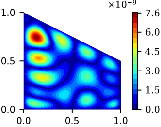
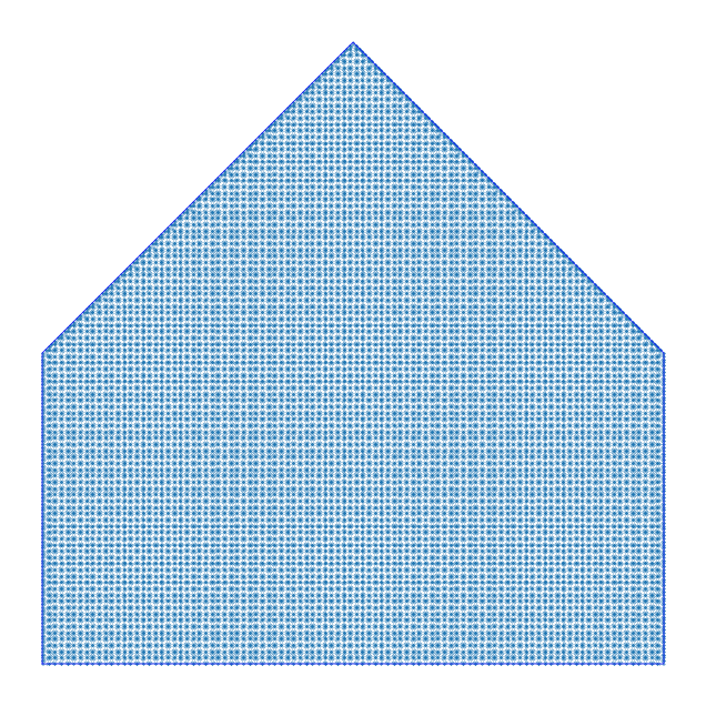
The exact solution to this problem is the signed distance function to the boundary $\Gamma$. Given the ridges (along the medial axis) that develop in the $C^{0}$ (nonsmooth) exact solution, this is a challenging problem for PINNs. A refined set of collocation points is used in the model training. Figure 22(b) shows the $14,382$ collocation points used for training. A very dense grid of testing points, which is shown in Fig. 22(c), is used for predictions against the exact solution. The network architecture 4–30–30–30–30–1 is used. Training was performed with Adam for $2,000$ epochs, and then with L-BFGS ($\log$ of the loss function) for $5,000$ epochs. Figure 22(a) shows the training loss; the loss at the end of training is $5\times 10^{-4}$. Figure 22(f) depicts the absolute error between the exact solution and the prediction by PINN. The PINN solution is highly accurate across most of the pentagon, except near its centroid. The maximum pointwise absolute error is ${\cal O}(10^{-2})$.

(a)

(b)

(c)

(d)

(e)

(f)

Figure 22: PINN solution for the Eikonal problem for a pentagon. Network architecture is 5–30–30–30–30–1. (a) Training loss; (b) Collocation points for training; (c) Testing points for predictions; (d) Exact solution, $u$; (e) PINN solution, $u_{\theta}^{\mathrm{TFI}}$; and (f) Absolute error of PINN, $|u-u_{\theta}^{\mathrm{TFI}}|$;

7 Conclusions

In this paper, we proposed a Wachspress-based transfinite formulation for physics-informed neural networks to exactly enforce Dirichlet boundary conditions over convex polygonal domains. This overcomes the primary limitation of approximate distance functions [15]—unbounded Laplacian at the vertices of a polygonal domain—in physics-informed neural networks [1]. Boolean sum operation, which is used for bilinear Coons transfinite interpolation on the square [24], cannot be directly extended to convex polygonal domains with four (quadrilateral) or more sides. In this work, the transfinite interpolant was formed by using Wachspress coordinates as the blending functions in the formula that is based on a projection onto the faces of a convex domain [14]. This generalizes bilinear Coons transfinite interpolation from a rectangular domain to a convex polygonal domain. For a polygonal domain $P$ and prescribed boundary function $\mathcal{B}$ on $\partial P$, the transfinite interpolant of $\mathcal{B}$, $g:\bar{P}\to C^{0}(\bar{P})$, was viewed as a lifting that extended the boundary function to the interior of the domain. To construct the transfinite trial function, we formed the difference between the neural network’s output and the extension of its boundary restriction to the interior of the polygonal domain, and then added $g$ to it. Since the restriction of the trial function to the boundary yielded $\mathcal{B}$, strong enforcement of Dirichlet boundary conditions was ensured.

On convex polygonal domains, Wachspress coordinates served as a geometric feature map that encoded the boundary edges. The spatial coordinates of a point, $\bm{x}\in\bar{P}$, was mapped to Wachspress coordinates, $\bm{x}\mapsto\bm{\lambda}$, which resided in the geometric feature (map) layer of the neural network architecture. In doing so, we showed that a framework emerged for solving Poisson problems on parametrized convex geometries using neural networks. In particular, the family of convex quadrilaterals with one vertex at $\bigl(1,(1+p)/2\bigr)$ $(p\in[0,1])$ was embedded in a curved hexahedron that was mapped to a cube. Besides the utility of this capability to solve partial differential equations using physics-informed neural networks, ideas emanating from this approach may also be valuable in the development of geometry-aware neural operators [4, 3, 65].

The advance introduced in this paper permitted choosing collocation points in physics-informed neural networks that were located very close to the boundary vertices, thereby overcoming a limitation from previous work [15]. Generalized barycentric coordinates are a natural choice as blending functions in the transfinite formula proposed in [14]. On convex polygons, Wachspress coordinates are $C^{\infty}$ (smooth) and their Laplacian are bounded, whereas they are unbounded for mean value coordinates. Hence, Wachspress coordinates were adopted in this study. The performance of the Wachspress-based transfinite formulation in PINNs was successfully assessed on several linear and nonlinear problems that included a harmonic problem over the unit square with highly oscillatory boundary conditions, a Poisson problem over a parametrized quadrilateral, an inverse heat conduction problem, and the nonlinear Eikonal equation for the distance function to the boundary of a pentagonal domain. Comparisons of the PINN predictions (absolute error in $u$ and $L^{2}$ norm of the gradient of the error) were made with the exact solution (when available) or with reference finite element solutions that were computed using the Abaqus™ finite element software package [44]. We demonstrated the sound accuracy of collocation-based PINNs and deep Ritz on convex polygonal domains, and showed that model training over a square domain delivered accurate solutions even when interior training points were arbitrarily close to the boundary vertices.

The proposed approach to exactly enforce Dirichlet boundary conditions is also suitable for solving linear eigenvalue problems over non-Cartesian (convex polygonal) geometries with the deep Ritz (Rayleigh quotient) method. In addition, for a convex polygon $P$, if $w(\bm{x}):=h(\bm{x})-\mathscr{L}[h(\bm{x})]$ for $\bm{x}\in\bar{P}$ and $0$ otherwise, we then observe that $w(\bm{x})\in C^{0}({\mathbb{R}}^{2})$ is compactly-supported and is a kinematically admissible test function that is suitable in domain-decomposition based variational PINNs. Here, $h(\bm{x})$ can be chosen to be any bivariate function, including polynomials, sines and cosines, or even the neural network’s output with assigned weights and biases. Furthermore, extensions of the proposed formulation to convex polyhedra and hypercubes in ${\mathbb{R}}^{n}$, and to nonconvex polygonal domains are also of interest. For the former, transfinite formula for convex polyhedra are provided in [14] and Matlab™ code to compute Wachspress coordinates in three dimensions is available [46]. For the latter, generalized barycentric coordinates on nonconvex polygon such as metric coordinates [66, 67] and variational barycentric coordinates (uses neural fields) [68] are worth exploring. Such topics offer potential directions for future research.

References

- \bibcommenthead
- Raissi et al. [2019] Raissi, M., Perdikaris, P., Karniadakis, G.E.: Physics-informed neural networks: A deep learning framework for forward and inverse problems involving nonlinear partial differential equations. Journal of Computational Physics 378, 686–707 (2019)
- Lu et al. [2021] Lu, L., Jin, P., Pang, G., Zhang, Z., Karniadakis, G.E.: Learning nonlinear operators via DeepONet based on the universal approximation theorem of operators. Nature Machine Intelligence 3(3), 218–229 (2021)
- Li et al. [2020] Li, Z., Kovachki, N., Azizzadenesheli, K., Liu, B., Bhattacharya, K., Stuart, A., Anandkumar, A.: Fourier neural operator for parametric partial differential equations (2020) arXiv:2010.08895
- Lu et al. [2021] Lu, L., Meng, X., Mao, Z., Karniadakis, G.E.: DeepXDE: A deep learning library for solving differential equations. SIAM Review 63(1), 208–228 (2021)
- Dissanayake and Phan-Thien [1994] Dissanayake, M.W.M.G., Phan-Thien, N.: Neural-network-based approximations for solving partial differential equations. Communications in Numerical Methods in Engineering 10(3), 195–201 (1994)
- Lagaris et al. [1998] Lagaris, I.E., Likas, A., Fotiadis, D.I.: Artifical neural networks for solving ordinary and partial differential equations. IEEE Transactions on Neural Networks 9(5), 987–1000 (1998)
- Toscano et al. [2025] Toscano, J.D., Oommen, V., Varghese, A.J., Zou, Z., Ahmadi Daryakenari, N., Wu, C., Karniadakis, G.E.: From PINNs to PIKANs: recent advances in physics-informed machine learning. Machine Learning for Computational Science and Engineering 1(1), 1–43 (2025)
- Fuks and Tchelepi [2020] Fuks, O., Tchelepi, H.A.: Limitations of physics informed machine learning for nonlinear two-phase transport in porous media. Journal of Machine Learning for Modeling and Computing 1(1) (2020)
- Krishnapriyan et al. [2021] Krishnapriyan, A., Gholami, A., Zhe, S., Kirby, R., Mahoney, M.W.: Characterizing possible failure modes in physics-informed neural networks. Advances in Neural Information Processing Systems 34, 26548–26560 (2021)
- Wang et al. [2021] Wang, S., Teng, Y., Perdikaris, P.: Understanding and mitigating gradient flow pathologies in physics-informed neural networks. SIAM Journal on Scientific Computing 43(5), 3055–3081 (2021)
- Wang et al. [2022] Wang, S., Yu, X., Perdikaris, P.: When and why PINNs fail to train: A neural tangent kernel perspective. Journal of Computational Physics 449, 110768 (2022)
- Rohrhofer et al. [2023] Rohrhofer, F.M., Posch, S., Gößnitzer, C., Geiger, B.C.: Data vs. physics: The apparent pareto front of physics-informed neural networks. IEEE Access 11, 86252–86261 (2023)
- Wachspress [2016] Wachspress, E.: Rational Bases and Generalized Barycentrics: Applications to Finite Elements and Graphics. Springer, Cham (2016)
- Randrianarivony [2011] Randrianarivony, M.: On transfinite interpolations with respect to convex domains. Computer Aided Geometric Design 28(2), 135–149 (2011)
- Sukumar and Srivastava [2022] Sukumar, N., Srivastava, A.: Exact imposition of boundary conditions with distance functions in physics-informed deep neural networks. Computer Methods in Applied Mechanics and Engineering 389, 114333 (2022)
- McFall and Mahan [2009] McFall, K.S., Mahan, J.R.: Artificial neural network method for solution of boundary value problems with exact satisfaction of arbitrary boundary conditions. IEEE Transactions on Neural Networks 20(8), 1221–1233 (2009)
- Lu et al. [2021] Lu, L., Pestourie, R., Yao, W., Wang, Z., Verdugo, F., Johnson, S.G.: Physics-informed neural networks with hard constraints for inverse design. SIAM Journal on Scientific Computing 43(6), 1105–1132 (2021)
- Yu et al. [2022] Yu, J., Lu, L., Meng, X., Karniadakis, G.E.: Gradient-enhanced physics-informed neural networks for forward and inverse PDE problems. Computer Methods in Applied Mechanics and Engineering 393, 114823 (2022)
- E and Yu [2018] E, W., Yu, B.: The deep Ritz method: a deep learning-based numerical algorithm for solving variational problems. Communications in Mathematics and Statistics 6(1), 1–12 (2018)
- Mortari [2017] Mortari, D.: The theory of connections: Connecting points. Mathematics 5(4), 57 (2017)
- Mortari and Leake [2019] Mortari, D., Leake, C.: The multivariate theory of connections. Mathematics 7(3), 296 (2019)
- Leake and Mortari [2020] Leake, C., Mortari, D.: Deep theory of functional connections: A new method for estimating the solutions of partial differential equations. Machine Learning and Knowledge Extraction 2(1), 37–55 (2020)
- Schiassi et al. [2021] Schiassi, E., Furfaro, R., Leake, C., De Florio, M., Johnston, H., Mortari, D.: Extreme theory of functional connections: A fast physics-informed neural network method for solving ordinary and partial differential equations. Neurocomputing 457, 334–356 (2021)
- Coons [1967] Coons, S.A.: Surfaces for Computer-Aided Design of Space Forms. Technical Report MAC-TR-41, Project MAC, MIT, Cambridge, MA (1967)
- Provatidis [2019] Provatidis, C.G.: Precursors of Isogeometric Analysis: Finite Elements, Boundary Elements, and Collocation Methods vol. 256. Springer, Cham, Switzerland (2019)
- Berg and Nyström [2018] Berg, J., Nyström, K.: A unified deep artificial neural network approach to partial differential equations in complex geometries. Neuralcomputing 317, 28–41 (2018)
- Rvachev and Sheiko [1995] Rvachev, V.L., Sheiko, T.I.: R-functions in boundary value problems in mechanics. Applied Mechanics Reviews 48(4), 151–188 (1995)
- Shapiro [2007] Shapiro, V.: Semi-analytic geometry with R-functions. Acta Numerica 16, 239–303 (2007)
- Berrone et al. [2023] Berrone, S., Canuto, C., Pintore, M., Sukumar, N.: Enforcing Dirichlet boundary conditions in physics-informed neural networks and variational physics-informed neural networks. Heliyon 9, 18820 (2023)
- Barschkis [2023] Barschkis, S.: Exact and soft boundary conditions in physics-informed neural networks for the variable coefficient Poisson equation (2023) arXiv:2310.02548
- Cooley et al. [2024] Cooley, M., Shankar, V., Kirby, R.M., Zhe, S.: Fourier PINNs: from strong boundary conditions to adaptive Fourier bases (2024) arXiv:2410.03496
- Anagnostopoulos et al. [2024] Anagnostopoulos, S.J., Toscano, J.D., Stergiopulos, N., Karniadakis, G.E.: Residual-based attention in physics-informed neural networks. Computer Methods in Applied Mechanics and Engineering 421, 116805 (2024)
- Gladstone et al. [2025] Gladstone, R.J., Nabian, M.A., Sukumar, N., Srivastava, A., Meidani, H.: FO-PINN: A first-order formulation for physics-informed neural networks. Engineering Analysis with Boundary Elements 174, 106161 (2025)
- Deguchi and Asai [2025] Deguchi, S., Asai, M.: Reliable and efficient inverse analysis using physics-informed neural networks with distance functions and adaptive weight tuning (2025) arXiv:2504.18091
- Zeinhofer et al. [2025] Zeinhofer, M., Masri, R., Mardal, K.-A.: A unified framework for the error analysis of physics-informed neural networks. IMA Journal of Numerical Analysis 45(5), 2988–3025 (2025)
- Gordon and Hall [1973] Gordon, W.J., Hall, C.A.: Transfinite element methods: blending-function interpolation over arbitrary curved element domains. Numerische Mathematik 21(2), 109–129 (1973)
- Barnhill et al. [1973] Barnhill, R.E., Birkhoff, G., Gordon, W.J.: Smooth interpolation in triangles. Journal of Approximation Theory 8(2), 114–128 (1973)
- Várady et al. [2011] Várady, T., Rockwood, A., Salvi, P.: Transfinite surface interpolation over irregular -sided domains. Computer-Aided Design 43(11), 1330–1340 (2011)
- Kato [1991] Kato, K.: Generation of -sided surface patches with holes. Computer-Aided Design 23(10), 676–683 (1991)
- Shepard [1968] Shepard, D.: A two-dimensional interpolation function for irregularly-spaced data. In: Proceedings of the 23rd ACM National Conference, pp. 517–524. Association for Computing Machinery, New York, NY (1968)
- Várady et al. [2024] Várady, T., Salvi, P., Vaitkus, M.: Genuine multi-sided parametric surface patches–a survey. Computer-Aided Design 110, 102286 (2024)
- Floater [2015] Floater, M.S.: Generalized barycentric coordinates and applications. Acta Numerica 24, 161–214 (2015)
- Hormann and Sukumar [2017] Hormann, K., Sukumar, N. (eds.): Generalized Barycentric Coordinates in Computer Graphics and Computational Mechanics. CRC Press, New York, NY (2017)
- Dassault Systèmes Simulia, Corp. [2025] Dassault Systèmes Simulia, Corp.: Abaqus Analysis User’s Guide. Dassault Systèmes Simulia, Corp., Providence, RI, USA (2025)
- Meyer et al. [2002] Meyer, M., Barr, A., Lee, H., Desbrun, M.: Generalized barycentric coordinates on irregular polygons. Journal of Graphics Tools 7(1), 13–22 (2002)
- Floater et al. [2014] Floater, M., Gillette, A., Sukumar, N.: Gradient bounds for Wachspress coordinates on polytopes. SIAM Journal on Numerical Analysis 52(1), 515–532 (2014)
- Dieci et al. [2024] Dieci, L., Difonzo, F.V., Sukumar, N.: Nonnegative moment coordinates on finite element geometries. Mathematics in Engineering 6(1), 81–99 (2024)
- Floater [2003] Floater, M.S.: Mean value coordinates. Computer Aided Geometric Design 20(1), 19–27 (2003)
- Dong and Ni [2021] Dong, S., Ni, N.: A method for representing periodic functions and enforcing exactly periodic boundary conditions with deep neural networks. Journal of Computational Physics 435, 110242 (2021)
- Hormann and Floater [2006] Hormann, K., Floater, M.S.: Mean value coordinates for arbitrary planar polygons. ACM Transactions on Graphics 25(4), 1424–1441 (2006)
- Joshi et al. [2007] Joshi, P., Meyer, M., DeRose, T., Green, B., Sanocki, T.: Harmonic coordinates for character articulation. ACM Transactions on Graphics 26(3), 71 (2007)
- Paszke et al. [2019] Paszke, A., Gross, S., Massa, F., Lerer, A., Bradbury, J., Chanan, G., Killeen, T., Lin, Z., Gimelshein, N., Antiga, L., Desmaison, A., Kopf, A., Yang, E., DeVito, Z., Raison, M., Tejani, A., Chilamkurthy, S., Steiner, B., Fang, L., Bai, J., Chintala, S.: PyTorch: An Imperative Style, High-Performance Deep Learning Library. In: Wallach, H., Larochelle, H., Beygelzimer, A., d’Alché-Buc, F., Fox, E., Garnett, R. (eds.) Advances in Neural Information Processing Systems, vol. 32, pp. 8024–8035. Curran Associates, Inc., Red Hook, NY (2019)
- McClenny and Braga-Neto [2023] McClenny, L.D., Braga-Neto, U.M.: Self-adaptive physics-informed neural networks. Journal of Computational Physics 474, 111722 (2023)
- Rathore et al. [2024] Rathore, P., Lei, W., Frangella, Z., Lu, L., Udell, M.: Challenges in training PINNs: A loss landscape perspective. In: Proceedings of the 41st International Conference on Machine Learning, pp. 42159–42191 (2024)
- Urbán et al. [2025] Urbán, J.F., Stefanou, P., Pons, J.A.: Unveiling the optimization process of physics informed neural networks: How accurate and competitive can PINNs be? Journal of Computational Physics 523, 113656 (2025)
- Jnini and Vella [2025] Jnini, A., Vella, F.: Dual natural gradient descent for scalable training of physics-informed neural networks (2025) arXiv:2505.21404
- Kiyani et al. [2025] Kiyani, E., Shukla, K., Urbán, J.F., Darbon, J., Karniadakis, G.E.: Optimizing the optimizer for physics-informed neural networks and Kolmogorov–Arnold networks. Computer Methods in Applied Mechanics and Engineering 446, 118308 (2025)
- Wang et al. [2025] Wang, S., Bhartari, A.K., Li, B., Perdikaris, P.: Gradient alignment in physics-informed neural networks: A second-order optimization perspective (2025) arXiv:2502.00604
- Gopal and Trefethen [2019a] Gopal, A., Trefethen, L.N.: Solving Laplace problems with corner singularities via rational functions. SIAM Journal on Numerical Analysis 57(5), 2074–2094 (2019)
- Gopal and Trefethen [2019b] Gopal, A., Trefethen, L.N.: New Laplace and Helmholtz solvers. Proceedings of the National Academy of Sciences 116(21), 10223–10225 (2019)
- Trefethen [2020] Trefethen, L.N.: Lightning Laplace solver (2020). https://people.maths.ox.ac.uk/trefethen/lightning.html
- Sitzmann et al. [2020] Sitzmann, V., Martel, J., Bergman, A., Lindell, D., Wetzstein, G.: Implicit neural representations with periodic activation functions. Advances in Neural Information Processing Systems 33, 7462–7473 (2020)
- Xiao and Gimbutas [2010] Xiao, H., Gimbutas, Z.: A numerical algorithm for the construction of efficient quadrature rules in two and higher dimensions. Computers & Mathematics with Applications 59(2), 663–676 (2010)
- Berrone et al. [2022] Berrone, S., Canuto, C., Pintore, M.: Variational physics informed neural networks: the role of quadratures and test functions. Journal of Scientific Computing 92(3), 1–27 (2022)
- Li et al. [2023] Li, Z., Huang, D.Z., Liu, B., Anandkumar, A.: Fourier neural operator with learned deformations for PDEs on general geometries. Journal of Machine Learning Research 24(388), 1–26 (2023)
- Malsch et al. [2005] Malsch, E.A., Lin, J.J., Dasgupta, G.: Smooth two-dimensional interpolants: A recipe for all polygons. Journal of Graphics Tools 10(2), 27–39 (2005)
- Sukumar and Malsch [2006] Sukumar, N., Malsch, E.A.: Recent advances in the construction of polygonal finite element interpolants. Archives of Computational Methods in Engineering 13(1), 129–163 (2006)
- Dodik et al. [2023] Dodik, A., Stein, O., Sitzmann, V., Solomon, J.: Variational barycentric coordinates. ACM Transactions on Graphics 42(6), 1–16 (2023)