A Branch-and-Price Algorithm for Fast and Equitable Last-Mile Relief Aid Distribution

Abstract

The distribution of relief supplies to shelters is a critical aspect of post-disaster humanitarian logistics. In major disasters, prepositioned supplies often fall short of meeting all demands. We address the problem of planning vehicle routes from a distribution center to shelters while allocating limited relief supplies. To balance efficiency and equity, we formulate a bi-objective problem: minimizing a Gini-index-based measure of inequity in unsatisfied demand for fair distribution and minimizing total travel time for timely delivery. We propose a Mixed Integer Programming (MIP) model and use the $\epsilon$-constraint method to handle the bi-objective nature. By deriving mathematical properties of the optimal solution, we introduce valid inequalities and design an algorithm for optimal delivery allocations given feasible vehicle routes. A branch-and-price (B&P) algorithm is developed to solve the problem efficiently. Computational tests on realistic datasets from a past earthquake in Van, Turkey, and predicted data for Istanbul’s Kartal region show that the B&P algorithm significantly outperforms commercial MIP solvers. Our bi-objective approach reduces aid distribution inequity by 34% without compromising efficiency. Results indicate that when time constraints are very loose or tight, lexicographic optimization prioritizing demand coverage over fairness is effective. For moderately restrictive time constraints, a balanced approach is essential to avoid inequitable outcomes.

Keywords: Humanitarian logistics, Equitable aid distribution, Multi-objective, Branch-and-Price

1 Introduction

After a disaster, affected individuals urgently need core relief items such as drinking water, food, quilts, blankets, sleeping sacks, jackets, tents, lighting equipment, medical goods, and other essential non-food items (UNHCR, 2024). These items are typically provided at temporary shelters where disaster-impacted individuals find refuge after the catastrophic event. In the devastating Maras earthquakes that struck Turkey in February 2023, the impact was profound, resulting in over 54,000 fatalities, more than 100,000 individuals injured, and an additional 2.5 million people in need of shelter across Southeastern Turkey and Northwestern Syria. During the initial response phase, emergency tents were distributed to those affected, eventually leading to the establishment of tent cities spanning 11 provinces in Southeastern and Eastern Turkey. Over time, the affected population transitioned to temporary housing solutions by establishing container cities with better infrastructure and services. By May 2023, over 400 tent cities and numerous container settlements with a collective capacity of approximately 100,000 containers were accommodating nearly one million displaced individuals.

In large-scale disasters like the Maras earthquakes, logistical challenges are immense due to limited resources and compromised accessibility during the initial stages of the crisis. Given the impossibility of addressing the needs of all affected individuals simultaneously and the complexity of the operations, developing strategies and solutions for equitable and efficient distribution of aid is vital. Governmental and non-governmental organizations typically store inventory in one or more depots and assign a set of shelters to each depot as part of their disaster preparedness plan. These depots are strategically located based on geographic coverage, accessibility, risk assessment, and proximity to vulnerable populations to ensure efficient and swift disaster response. During the early phase of disaster response, only locally prepositioned supplies are available for distribution.

In large-scale disasters like the Maras earthquakes, logistical challenges arise from limited resources and restricted accessibility during the crisis’s initial stages. Addressing all affected individuals simultaneously is impossible, making strategies for equitable and efficient aid distribution crucial. Governmental and non-governmental organizations typically store inventory in depots and assign shelters to each as part of disaster preparedness. These depots are strategically positioned based on geographic coverage, accessibility, risk assessment, and proximity to vulnerable populations to enable swift and efficient responses. In the early disaster phase, only locally prepositioned supplies are available for distribution. The scarce supplies should be delivered swiftly to alleviate the suffering (Hu et al., 2019).

The distribution of commodities to the shelters is based on the needs, information about the state of the road network, and the available number of vehicles together with their capacities, drivers, and volunteers gathered during an early assessment. This raises the question of how to efficiently allocate and distribute the relief goods to the shelters. If demands at all shelters could be fulfilled or the delivery amount to each shelter is determined at first, then the distribution decisions would constitute a classical vehicle routing problem (VRP). However, optimizing the relief amounts to be delivered to the shelters and the routes of the vehicles simulatenously may provide a better solution. This is the problem we address in our study.

In the early hours of the disaster, supply is scarce and not all demand can be satisfied. For instance, in the immediate aftermath of the Maras earthquakes in 2023, provinces such as Hatay and Adıyaman were left with a large amount of unsatisfied demand, whereas other provinces, such as Maras and Gaziantep, were more advantageous. In situations where part of the needs of beneficiaries must remain unfulfilled, “effectiveness” or “efficiency” cannot be the only goal; equity becomes an essential consideration.

Equitable relief distribution remains an open research area in operations research and humanitarian operations. This paper develops and solves a bi-objective optimization model as the basis for a decision support tool to help aid agencies design effective and equitable distribution plans. The model addresses distributing supplies from a single depot by dispatching available vehicles to shelters. It involves (i) determining the delivery amount to each shelter to partially or fully meet its demand and (ii) planning vehicle routes while accounting for road damages and accessibility. Figure 1 illustrates the structure of a solution by a small example.

Figure 1: Example of three vehicle routes (shown with different line types) delivering to shelters from a single depot. Numbers above each shelter show delivered amounts and corresponding demands, with demand satisfaction varying: 100% for the two rightmost shelters, but only 50% for the leftmost.

Within a bi-objective framework for determining Pareto-optimal solutions, we consider two largely conflicting objectives. The first objective aims to maximize the efficiency of the operation by minimizing the overall transportation time of the vehicles. In addition, we also impose a time limit for the completion of each individual vehicle route to achieve a service guarantee. The second objective evaluates both the total (or average) unsatisfied demand and the degree of inequity in its distribution among the affected population.

Evaluation measures for allocation of benefits to the individuals of a population have been proposed under the name of Social Welfare Functions (SWFs) (see Karsu and Morton (2015), Adler (2019), Chen and Hooker (2021)). In this paper, we apply a special SWF, defined as a weighted sum of two components: (i) average unsatisfied demand per victim and (ii) Gini’s mean absolute difference of the values of unsatisfied demand across all victims. Gini’s mean absolute difference builds on the well-known Gini index, arguably the most prominent inequity measure in the economic literature. For studies that use Gini index-related measures in operation research, please refer to Section 2.2.

The problem presented in this study extends the classical Capacitated Vehicle Routing Problem (CVRP) by determining the delivery amounts at each location, while considering service level constraints and optimizing for two objectives. Although our focus is on humanitarian logistics applications, it is worth mentioning that CVRP extensions addressing both efficiency and equity are also relevant in commercial logistics as exemplified by Toth and Vigo (2014). Vidal et al. (2020) highlighted the desirability of incorporating appropriate equity measures to capture service equity in vehicle routing problems. Matl et al. (2017) reviewed and analyzed equity measures in vehicle routing models, proposing the Gini index as a promising measure for capturing inequity in VRPs.

To our knowledge, no prior research has tackled a bi-objective problem that integrates explicit routing, delivery amount decisions, and equity considerations. More importantly, our proposed problem and algorithm offer practical value, helping humanitarian operations managers allocate scarce resources more effectively and equitably. By optimizing post-disaster resource distribution, we aim to ensure equitable access to essential supplies and support community recovery. Our study contributes to the VRP and humanitarian logistics literature as follows: 1) We incorporate a social welfare function based on the Gini index to balance effectiveness and equity in relief distribution. 2) We propose a bi-objective VRP-based MIP formulation, using the $\epsilon$-constraint method to address efficiency and equity trade-offs. 3) We derive mathematical properties of optimal deliveries. Based on these properties, we introduce two novel valid inequalities to tighten the LP relaxation of the model, significantly accelerating our column generation approach. 4) We develop an efficient solution approach to address computational challenges of a Gini-index-based objective, including a column generation method and a GRASP heuristic for the pricing problem. 5) We design a Branch-and-Price (B&P) algorithm, enhanced with a heuristic to generate an initial set of columns leading to a feasible solution. 6) Our computational study uses datasets from Istanbul’s Kartal district and Turkey’s Van province, offering insights into the trade-offs between objectives and the price of fairness in real-world scenarios.

The rest of the article is organized as follows. Section 2 discusses related works. The formal problem definition, a mathematical model, the social welfare objective function, as well as properties of the optimal solution are presented in Section 3. In Section 4, we introduce our exact solution method. Section 5 is devoted to our computational experiments. Finally, we conclude our work and discuss future research directions in Section 6.

2 Literature review

2.1 Relief aid distribution

In recent years, numerous articles focused on the challenges associated with last-mile disaster relief, with regard to various aspects such as relief aid distribution (Lin et al. (2011), Penna et al. (2018), Bruni et al. (2018), Sheu (2014)), medical/technical crew routing and team deployment (Talarico et al. (2015), Duque et al. (2016), Chen and Miller-Hooks (2012)), road restoration post-disaster networks (Duque et al. (2016), Akbari et al. (2021), Ajam et al. (2022)) or victim evacuation from affected areas (Zhu et al. (2019), Molina et al. (2018)). A considerable portion of these papers develops models with multiple objectives to account for the diverse evaluation criteria used in humanitarian operations. Works such as Lin et al. (2011), Chang et al. (2014), Wang et al. (2014), Huang et al. (2015), Molina et al. (2018), Ferrer et al. (2018), cf. also the survey Gutjahr and Nolz (2016), exemplify this approach. For multi-objective vehicle routing in a more general context, we refer to Jozefowiez et al. (2008); Zajac and Huber (2021). For comprehensive insights into mathematical models for the humanitarian supply chain and emergency logistics management, we recommend reviewing works such as Kundu et al. (2022), Habib et al. (2016), Özdamar and Ertem (2015) or Anaya-Arenas et al. (2014).

An early paper by Balcik et al. (2008) addressed relief supply allocation and vehicle routing, proposing a two-phase approach to minimize logistics and penalty costs for unmet or delayed demands. Their algorithm first determines delivery schedules, followed by inventory allocation. Nolz et al. (2011) focused on post-disaster drinking water distribution, aiming to reduce operational risk, water access travel time, and total vehicle travel time. Chang et al. (2014) implemented a multi-objective genetic algorithm for relief distribution during Taiwan’s Chi-Chi earthquake. Huang et al. (2015) studied aid distribution and allocation, emphasizing life-saving utility, fairness, and delay costs. Moreno et al. (2018) optimized distribution center locations and fleet sizing under uncertainty with a two-stage stochastic model to reduce logistics costs and human suffering. Vehicle routing is a crucial aspect of last-mile delivery, and for articles focusing on the vehicle routing problem in humanitarian operations, readers can refer to the review by Anuar et al. (2021).

While many studies concentrate on the effective and efficient distribution of relief aid in post-disaster settings, none of the mentioned studies address the equity of distributed aids. This work stands out from previous efforts by considering both the efficiency and equity of distributions.

2.2 Equity in humanitarian logistics

The humanitarian logistics literature increasingly addresses equity (fairness) in post-disaster logistics, particularly concerning emergency response times. Holguín-Veras et al. (2013) introduced deprivation cost to quantify human suffering in these contexts. However, Gutjahr and Fischer (2018) highlighted that solely minimizing total deprivation costs, although initially expected to promote equitable solutions, was still insufficient to ensure equity. To address this, they proposed a measure based on Gini’s mean absolute difference in deprivation costs, an aggregation function (Kostreva et al. (2004)) that balances effectiveness and equity. Their case study on the 2015 Nepal earthquake demonstrated significant equity gains with minimal effectiveness losses. Similarly, Alem et al. (2022) used the Gini coefficient to optimize the equity-effectiveness trade-off in location-allocation problems, introducing valid inequalities and a clustering-based Lorenz curve construction to streamline constraints and variables. Their model was tested on data from flood and landslide disasters in Rio de Janeiro state, Brazil.

In recent years, the Gini index and Gini’s mean absolute difference have been utilized to incorporate fairness considerations in various problems such as relief aid distribution in disaster response (Gutjahr and Fischer (2018), Park and Berenguer (2020)), humanitarian food distribution (Eisenhandler and Tzur (2019b), Eisenhandler and Tzur (2019a)), shelter location in disaster preparedness (Mostajabdaveh et al. (2019), Gutjahr (2021)), and equitable vaccine distribution to control an epidemic (Enayati and Özaltın (2020), Gutjahr (2023)). For a recent and comprehensive examination of equity measures in Operations Research studies, including Gini-related measures, readers are referred to Chen and Hooker (2021).

Several papers investigated humanitarian logistics problems using other approaches for ensuring equity, such as the maxmin function (Rawlsian approach). Campbell et al. (2008) were among the first to apply equity concepts to disaster relief supply distribution, introducing an equity-related objective defined as minimizing maximum arrival time to demand points. They employed local search heuristics to obtain significantly different solutions compared to conventional objectives. Some articles use models representing uncertainty, see, for example, Noyan et al. (2015), Noyan and Kahvecioğlu (2018), Sabouhi et al. (2018), Fianu and Davis (2018), Cheng et al. (2021), and Li et al. (2024). Other works examine the relief item distribution problem in a multi-period setting; see Yu et al. (2018), Huang and Rafiei (2019), Çankaya et al. (2019), and Ekici and Özener (2020). We refer the reader to the review by Dönmez et al. (2022) for fairness in humanitarian logistics operations. Our work differs from the studies mentioned above by specifically addressing the problem of aid distribution, and by using a Gini-index-related metric.

In order to locate our paper within the existing literature, we can use the classification in the recent survey by Vidal et al. (2020). Therein, regarding models with equity objectives, three types of papers are distinguished: papers dealing with (i) workload balance, (ii) service equity, or (iii) collaborative planning. Our current work addresses the second of these types, service equity. In this category, Vidal et al. (2020) indicate only two publications, namely Balcik et al. (2010) and Huang et al. (2012). The survey by Balcik et al. (2010) is close to our work as it focuses on equity considerations in vehicle routing. The Gini index, the main metric concept of the current paper, is already mentioned. Moreover, the authors already refer to supplies as equity determinants, as opposed to arrival times or similar measures which prevail in the most other articles on equitable routing. However, no publication dealing with equitable supply by a Gini-based approach is referred to in the survey.

Huang et al. (2012) studied equitable aid distribution, but defined equity in terms of standard deviation and of maximum pairwise difference between individual service levels, where the service level is determined for each aid recipient from delivery speed and delivery amount. More recently, Soghrati Ghasbeh et al. (2022) focused on maximizing equity and minimizing response time in post-disaster relief aid distribution, where equity is addressed by minimizing a weighted sum of unmet demand for non-emergency commodities. Both Huang et al. (2012) and Soghrati Ghasbeh et al. (2022) use equity concepts that are different from our approach as they do not rely on the Gini index.

Eisenhandler and Tzur (2019b) introduced the humanitarian pickup and distribution problem for food donation logistics, addressing site selection, routing, and allocation under capacity and working-hour constraints. The objective function combines total delivered units with a Gini-based equity measure. A heuristic method was tested on data from food banks in Israel and Houston, Texas. Eisenhandler and Tzur (2019a) extended this work with a segment-based formulation and a new heuristic to handle complex scenarios, including multi-vehicle cases and time windows. Our relief distribution problem shares similarities with these studies but differs in its use of a more general equity measure, its application context, structure, and solution method. Specifically, we address multi-vehicle cases with a bi-objective formulation for equity and travel time, assuming all demand points require service. Importantly, we compute exact solutions, tackling the challenge noted in Eisenhandler and Tzur (2019a), where the authors state that solving their model by an approach using column generation and branch-and-price would be a complex task.

Avishan et al. (2023) address the problem of routing relief logistics teams after a major disaster. Their model decides on the service time of teams at each location and considers the equity of the service time received by affected sites. Equity is indirectly managed through a utility function, where utility decreases each time unit when the service time exceeds a site’s critical need. The study utilizes adjustable robust optimization to address the uncertainty in the travel times of relief teams. To solve the problem efficiently, a heuristic approach is proposed. There are notable differences with our model. We address the frequent case where relief supplies fall short of demand. Contrary to the approach based on service time, our study explicitly calculates the amount of relief supplies delivered to each location. Additionally, we directly consider equity. Furthermore, instead of relying on heuristics, we employ an efficient exact algorithm to solve the problem.

In summary, the literature on relief aid distribution that combines vehicle routing decisions with decisions on deliveries while considering equity remains relatively limited. Here, we introduce a novel bi-objective optimization model for determining a distribution plan that dictates vehicle routes and delivery quantities to shelters. This model aims to minimize two objectives: (i) total traveling time and (ii) inequity of relief supply distribution. Notably, none of the previously mentioned studies have presented an exact solution method that efficiently addresses problems of similar structure for real-world application sizes. Our problem focuses on the post-disaster response stage, necessitating swift identification of solutions. We believe that our developed efficient branch-and-price method for equitable relief item routing constitutes a significant contribution in terms of both practical utility and methodological advancement. Table 1 surveys related publications in comparison to our work.

Study	Multi- Objective	Equity Measure	Routing Aspects	Decision on Delivery Quantities	Method
Campbell et al. (2008)	No	MinMax Arrival Time	VRP/TSP with vehicle capacity	No	Local search with insertion/ improvement
Huang et al. (2012)	No	Min Service level differences	Vehicle-to-route assignment	Yes	CPLEX / GRASP
Huang et al. (2015)	Yes, Max lifesaving utility, Min delay cost, Min variance of demand fill rates	Demand fill rate variance	Network flow	Yes	Convex quadratic network flow, VI algorithm
Moreno et al. (2018)	Yes, Min deprivation costs, Min logistics costs	Deprivation costs	Vehicle-to-node assignment	Yes	Two-stage stochastic model, heuristics
Eisenhandler and Tzur (2019a)	Yes, Max food allocation, Max equity of food distribution	Gini-related measure	Single vehicle Pickup and delivery, Vehicle capacity	Yes	Large neighborhood search
Eisenhandler and Tzur (2019b)	Yes, Max food allocation, Max equity of food distribution	Gini-related measure	Pickup and delivery, Vehicle capacity, Time windows	Yes	Matheuristic
Ghasbeh et al. (2022)	Yes, Min unmet demand, Min response time	Weighted unmet demand	Location- routing	Yes	ALNS and local search
Avishan et al. (2023)	Yes, Min unmet demand, Min max service time difference	Utility of service time	Pickup and delivery, Time windows	No	Robust optimization, Heuristic
Ours	Yes, Min total travel time, Min inequity of relief supply distribution	Gini-related measure	VRP with vehicle capacity and travel time limit	Yes	Branch- and-Price

Table 1: Summary of objectives, equity measures, routing decisions, and methodologies in relief aid distribution studies considering equity

3 Problem definition and mathematical models

For the response phase after a disaster, we investigate the problem of planning vehicle routes between a depot and shelter locations while simultaneously assigning relief supplies to the shelters. A depot is a distribution center where relief items are pre-positioned in preparation for a disaster. Shelters are assumed to receive supplies from a single depot, as it is conventional in practice for a shelter to be assigned to a single distribution center.

The problem is defined on a directed graph $G=(V,A)$. The node set $V=\{0,...,n,n+1\}$ contains the depot that is represented by both node 0 and node $n+1$, and $n$ shelters. We denote the set of all shelters as $V_{c}=V\setminus\{0,n+1\}$. The set $A$ is defined as $\{(i,j)\,|\,i,j\in V,\,i\neq j,\,i\neq n+1,\,j\neq 0\}$. To each edge $(i,j)$, a travel time $t_{i,j}$ is assigned, which is calculated as the time for traversing the shortest path between $i$ and $j$ in the post-disaster road network. We assume that the necessary information on the road network, such as information on time required for road restoration and traffic condition, has already been collected during an initial assessment phase and has been taken into account in the computation of the numbers $t_{i,j}$. Travel times are not necessarily symmetric, so $t_{i,j}$ needs not be equal to $t_{j,i}$.

Note that by the assumption above, the given road network graph has been extended to an (almost) complete graph $G$. While traversing edge $(i,j)$ of $G$, i.e., while traveling from node $i$ to node $j$, a route may physically pass through other nodes that lie on the shortest path between $i$ and $j$. This does not imply that the shelters located at these intermediate nodes are visited. For example, suppose the physical network consists of three nodes, a depot and two shelters indexed 1 and 2, that lie on one and the same straight road in the indicated order. Then a vehicle may start at the depot, visit shelter 1, visit shelter 2, and return then to the depot while passing through node 1 once again. In the graph $G$, where the depot is indexed as node 0 or node 3, this second passage does not count as a visit to shelter 1, since in $G$, the backward trip only corresponds to a traversal of edge (2,3), but neither of (2,1) nor of (1,3). We would also like to note that the triangle inequality might not hold in the original road network, but it holds in the complete graph G by definition of $t_{i,j}$, since if $t_{i,j}$ would be larger than $t_{i,k}+t_{k,j}$, then the path defining $t_{i,j}$ would not be a shortest path.

Each shelter $i$ requires an amount of relief supply, $d_{i}$, which is calculated by an assessment of the number of victims who need relief items at shelter location $i$. We are concerned with a single commodity, or equivalently, a package combining several commodities with fixed proportions that are composed according to the common needs of victims. We assume that only the prepositioned relief supply at the depot, $C$, is available for distribution among victims. Furthermore, we consider the (frequent) situation where the prepositioned supply $C$ is less than the total demand of shelters: $C<\sum_{i\in V_{c}}d_{i}$, which is the challenging case from the viewpoint of equity.

A fleet of $m$ homogeneous vehicles, each with a capacity of $Q$, is based at the depot. Each vehicle performs only one route that starts from the depot and visits some of the shelters on the post-disaster network. The total duration of each route has to be less than $\Psi$. Each shelter is allowed to be visited only once for the purpose of delivering goods; however, it can act as an intermediate node on a route. We do not allow split delivery, i.e., the demand of a shelter is (partially or completely) covered by at most one vehicle.

We address two objectives for the problem, time efficiency and unsatisfied demand. To represent time efficiency, we minimize the total relief response time, which is the sum of all vehicles’ traveling times. As for the second objective, we combine the average unsatisfied demand per victim with an equity measure: Gini’s mean absolute difference of unsatisfied demand ratios between individuals. A detailed explanation of this measure can be found in Section 3.2. Table 2 presents the notation for the problem’s parameters. In the following sections, we introduce a compact formulation of the problem.

Table 2: Parameters

Parameter	Definition
$Q$	Vehicle capacity
$d_{i}$	Demand for relief supplies at shelter node $i$
$D$	Total demand, $D=\sum_{i}d_{i}$
$t_{i,j}$	Time it takes to travel between nodes $i$ and $j$
$C$	Total amount of available relief supply
$\Psi$	Maximum delivery time (time when the last supply has to be delivered)
$m$	Number of vehicles

3.1 Mathematical model

To formulate our problem, we first follow the vehicle flow formulation for the VRP with maximum travel time duration. This formulation is easy to understand, implement, and adapt to additional assumptions. We refer to this formulation as the VF model in this work. The decision variables are as defined in Table 3.

Table 3: Decision Variables

Notation	Description	Variable type	Domain
$x_{i,j}$	1, if the vehicle directly travels from node $i$ to node $j$	binary	$\forall i,j\in V$
$v_{i}$	The amount of relief supply to node $i$	non-negative	$\forall i\in V_{c}$
$u_{i}$	The amount of delivered vehicle load when reaching node $i$	non-negative	$\forall i\in V_{c}$
$w_{i}$	The time that the vehicle visits node $i$, $u_{0}=0$	non-negative	$\forall i\in V$

$$\text{objective 1: }\min\> z_{1}=\sum_{(i,j)\in A}t_{i,j}{x_{i,j}}$$ (1)

$$\text{objective 2: }\min\> z_{2}=D\cdot{\cal I}(v)$$ (2)

s.t. $$\sum\limits_{j\in V\setminus\{0\}}{x_{i,j}}=1,\quad\forall i\in V_{c},$$ (3)

$$\sum\limits_{j\in V\setminus\{n+1\}}x_{j,i}=1,\qquad i\in V_{c},$$ (4)

$$\sum\limits_{j\in V\setminus\{0\}}x_{0,j}\leq m,$$ (5)

$$\sum\limits_{i\in V\setminus\{n+1\}}x_{i,n+1}\leq m,$$ (6)

$$v_{i}\leq d_{i},\qquad\forall i\in V_{c},$$ (7)

$$\sum\limits_{i\in V_{c}}v_{i}\leq C,$$ (8)

$$w_{j}\geq w_{i}+t_{i,j}-(1-x_{i,j})M,\qquad\forall i,j\in V,$$ (9)

$$w_{j}\leq\Psi,\qquad\forall j\in V_{c}$$ (10)

$$u_{j}\geq u_{i}+v_{i}-(1-x_{i,j})M,\qquad\forall i,j\in V_{c},$$ (11)

$$u_{j}\leq Q,\qquad\forall j\in V_{c}$$ (12)

$$x_{i,j}\in\{0,1\},\quad\forall(i,j)\in A,$$

$$v_{i},u_{i},w_{i}\geq 0\qquad\forall i\in V_{c}$$ (13)

The model starts with the two objective functions of our bi-objective problem, where objective 1 represents total traveling time, while objective 2 is the objective function expressing inequity of demand coverage. The inequity measure ${\cal I}={\cal I}(v)$ will be defined and explained in Section 3.2. Constraints (3) ensure that each shelter will be visited once. Constraints (4) impose ensure that a vehicle leaves a shelter exactly once. Constraints (5) and (6) make sure that not more than $m$ vehicles are in use. Constraints (7) and (8) guarantee that the delivered amount to a shelter does not exceed the shelter’s demand, and that the sum of the delivered amounts is less or equal to the total available relief supply at the depot, respectively. Constraints (9) calculate the visiting time of each shelter $i$, represented by variable $u_{i}$. Constraints (10) make sure that all shelters are visited before time $\Psi$ given that vehicles start at time 0. Constraints (11) calculate the vehicle load at the time of visiting shelter $i$, and Constraints (12) guarantee that the vehicle load does not exceed the vehicle capacity. Finally, Constraints (13) define the variables’ domains.

3.2 Representation of inequity

Unsatisfied demand in at least one shelter is an inevitable consequence of the situation considered in this paper, that of insufficient overall supply. A straightforward approach (called “utilitarian” in the literature) would simply minimize the total amount of unsatisfied demand. However, it is well-known that this approach often leads to very unbalanced distributions of the relief commodities, privileging parts of the population and grossly discriminating against other parts. Thus, in a situation of scarce resources, balancing the amount of relief supply delivered to shelter locations in a fair way plays a crucial role for achieving an allocation of supply that is ethically tenable and well-accepted by the population. Therefore, we do not restrict our second, coverage-related objective function to an evaluation of total coverage, but complement it by a second term: an equity measure expressing the degree to which the unsatisfied demand in the different shelters is fairly distributed. The well-known Gini index seems to be the most popular equity measure in the economic literature, so we have decided to build on this index.

In this way, we get two components for our second objective function: (i) an effectiveness term, representing the total (or, equivalently, average) unsatisfied demand and (ii) an inequity term, quantified by means of the Gini index concept, which judges the extent of inequity of the unsatisfied demand values across the population. The two terms are aggregated in the form of a weighted sum. This produces a social welfare function belonging to a class called inequity-averse aggregation functions (IAAFs) in Karsu and Morton (2015). For previous applications of the same measure, see Gutjahr and Fischer (2018), Mostajabdaveh et al. (2019) or Gutjahr (2023). Concerning a motivation of the way how our IAAF is constructed, we restrict us here to the remark that a weighted sum is obviously the most natural approach to combine the two basic terms. This approach has a long tradition in the literature: readers interested in an axiomatic justification of the chosen IAAF are referred to Porath and Gilboa (1994) and Argyris et al. (2022). Moreover, the weighted sum formula can also be derived from game-theoretic models, as shown in Schmidt and Wichardt (2019).

In a minimization problem concerning $N$ individual persons, indexed $\nu=1,\ldots,N$, let $c^{(\nu)}$ represent the cost or any alternative form of disutility encountered by individual $\nu$. In this study, $c^{(\nu)}$ quantifies the unsatisfied demand (detailed further below). We define our IAAF as ${\cal I}=\mu+\lambda\cdot\Delta$, where $\mu$ denotes the average cost, calculated as $\mu=\frac{1}{N}\sum_{\nu=1}^{N}c^{(\nu)}$, and $\Delta$ represents Gini’s mean absolute difference, defined as $\Delta=\frac{1}{N^{2}}\sum^{N}\limits_{\nu=1}\sum^{N}\limits_{\ell=1}|c^{(\nu)}-c^{(\ell)}|$, to measure the dispersion of individual costs. It is well-known that $\Delta=2\mu{\cal G}$, where ${\cal G}$ denotes the Gini index. To use Gini’s mean absolute difference $\Delta$ instead of the Gini index ${\cal G}$ as the second term has the advantages that $\Delta$ can be linearized, and that $\Delta$ is expressed in the same units as $\mu$, such that the weight factor $\lambda$ is a dimension-less constant.

For $0\leq\lambda\leq 1/2$, the measure ${\cal I}$ is guaranteed to be monotonous in the individual costs $c^{(\nu)}$ (this is Axiom 4 in Porath and Gilboa (1994)), which excludes implausible solutions where the value of ${\cal I}$ could be improved by increasing the costs of one or several individuals while keeping the costs of the other individuals unchanged. In our computational results, we choose $\lambda=1/2$.

In our study, we assume that the demand of each beneficiary is one unit, that is, $d_{i}$ represents the number of beneficiaries at shelter $i$. We define the unsatisfied demand of an individual $\nu$ at shelter $i$ as $c^{(\nu)}=1-v_{i}/d_{i}$, assuming equal distribution within each shelter. In particular, $c^{(\nu)}$ is identical for all individuals $\nu$ at shelter $i$ and can therefore be written as $c_{i}$ $(i\in V_{c})$. Note that this term is always non-negative since the delivery amount $v_{i}$ to shelter $i$ is less or equal to the demand $d_{i}$. Moreover, the total demand $D=\sum_{i}d_{i}$ is identical to the number $N$ of beneficiaries.

The quantities $\mu$ and $\Delta$ can be immediately calculated as follows.

$$\mu=\frac{1}{D}\sum_{i\in V_{c}}d_{i}\,c_{i}=\frac{1}{D}\sum_{i\in V_{c}}d_{i}\cdot(1-v_{i}/d_{i})=\frac{1}{D}\sum\limits_{i\in V_{c}}(d_{i}-v_{i})=1-\frac{1}{D}\sum\limits_{i\in V_{c}}v_{i},$$ (14)

$$\Delta=\frac{1}{D^{2}}\sum\limits_{i\in V_{c}}\sum\limits_{j\in V_{c}}d_{i}d_{j}\,|c_{i}-c_{j}|=\frac{1}{D^{2}}\sum\limits_{i\in V_{c}}\sum\limits_{j\in V_{c}}d_{i}d_{j}\,|v_{j}/d_{j}-v_{i}/d_{i}|=\frac{1}{D^{2}}\sum\limits_{i\in V_{c}}\sum\limits_{j\in V_{c}}|d_{i}v_{j}-d_{j}v_{i}|.$$ (15)

Please note that our inequity measure does not refer to inequity in demand satisfaction ratios between shelters, but between individuals. We multiply $\cal I$ by the constant $D$ and adopt the resulting expression as the inequity objective function in our problem.

$$D\cdot{\cal I}=\sum\limits_{i\in V_{c}}(d_{i}-v_{i})+\frac{\lambda}{D}\sum\limits_{i\in V_{c}}\sum\limits_{j\in V_{c}}|d_{i}v_{j}-d_{j}v_{i}|.$$ (16)

To linearize the non-linear term in the objective function, we introduce $2\cdot|V_{c}|^{2}$ new continuous variables alongside two sets of corresponding constraints. Specifically, we define auxiliary variables $\tau^{+}_{i,j}$ and $\tau^{-}_{i,j}$, where $\tau^{+}_{i,j}=\max\{0,(d_{i}v_{j}-d_{j}v_{i})\}$ and $\tau^{-}_{i,j}=\max\{0,-(d_{i}v_{j}-d_{j}v_{i})\}$ for every pair of $i,j\in V_{c}$. These variables allow us to express the objective function (16) as follows:

$$\sum_{i\in V_{c}}(d_{i}-v_{i})+\frac{\lambda}{D}\sum_{i\in V_{c}}\sum_{j\in V_{c}}(\tau^{+}_{i,j}+\tau^{-}_{i,j}),$$

where

$$\tau^{+}_{i,j}-\tau^{-}_{i,j} =d_{i}v_{j}-d_{j}v_{i}, \forall i,j\in V_{c},$$ (17)

$$\tau^{+}_{i,j},\tau^{-}_{i,j} \geq 0, \forall i,j\in V_{c}.$$ (18)

Note that in view of constraint (17) and the fact that both $\tau^{+}_{i,j}$ and $\tau^{-}_{i,j}$ have positive coefficients in our minimization objective, at most one of these variables will assume a positive value in the optimal solution.

3.3 Characteristics of the optimal solution

A feasible solution $X$ to our problem consists of two components: (i) a set of $m$ vehicle routes $K$ that meet the maximum route length constraint, and (ii) a specification of delivery quantities $v_{i}$ to the shelter locations that meet the vehicle capacity constraint and the limitation imposed by the amount of prepositioned relief items. Our first objective function (total traveling time) is already determined by the first component, while the second objective function (the IAAF of the uncovered demand) is exclusively determined by the second component. In this section, we assume the vehicle routes in solution $X$ are fixed, resulting in a constant total travel time. Our focus is on optimizing delivery quantities $v_{i}$ according to the second objective function (16). The set of all nodes that are visited by route $k$ will be denoted by $V_{k}$ $(k\in K)$. Then we have the problem

$$\min\quad D\cdot{\cal I}=\sum\limits_{i\in V_{c}}(d_{i}-v_{i})+\frac{\lambda}{D}\sum\limits_{i\in V_{c}}\sum\limits_{j\in V_{c}}|d_{i}v_{j}-d_{j}v_{i}|$$ (19)

$$\sum_{i\in V_{k}}v_{i}\leq Q\quad\forall k\in K$$ (20)

$$\sum_{i\in V_{c}}v_{i}\leq C$$ (21)

$$0\leq v_{i}\leq d_{i}\quad\forall i\in V_{c}$$ (22)

For each route $k\in K$, set $D_{k}=\sum_{i\in V_{k}}d_{i}$ and introduce variables $\xi_{k}=\sum_{i\in V_{k}}v_{i}$.

The proofs of the following results can be found in the Online Supplement.

Lemma 1. There is an optimal solution $v=(v_{i})$ of (19) – (22) for which within each set $V_{k}$, the $v_{i}$ are distributed demand-proportional, i.e. as $v_{i}=\xi_{k}\cdot\frac{d_{i}}{D_{k}}$ $(i\in V_{k},\,k\in K)$.

By Lemma 1, when looking for optimal solutions, we can restrict ourselves to solutions in which deliveries $v_{i}$ within each $V_{k}$ are given by $v_{i}=\xi_{k}\cdot\frac{d_{i}}{D_{k}}$ $(i\in V_{k},\,k\in K)$. Insertion into (19) – (22) yields the following optimization problem in the non-negative variables $\xi_{k}$:

$$\min_{\xi}\;\psi(\xi)=D\,{\cal I}=D-\sum_{k}\xi_{k}+\frac{\lambda}{D}\,\sum_{k\in K}\sum_{\ell\in K}|D_{\ell}\xi_{k}-D_{k}\xi_{\ell}|.$$ (23)

$$\mbox{s.t.}\;\>0\leq\xi_{k}\leq\min(Q,D_{k})\;\>\forall k,\quad\sum_{k\in K}\xi_{k}\leq C.$$ (24)

The following two propositions will allow a solution of (23) – (24) by simple arithmetic calculations:

Proposition 1.

If $\frac{D_{k}}{D}\leq\frac{Q}{C}$ for all $k\in K$, then the optimal solution of (23) – (24) is given by

$$\xi_{k}=\frac{C}{D}\cdot D_{k}\quad(k\in K),$$ (25)

which constitutes perfect equity.

Proposition 2.

If $\frac{D_{k}}{D}>\frac{Q}{C}$ for some $k\in K$, then in an optimal solution $\xi=(\xi_{1},\ldots,\xi_{m})$ of (23) – (24), it holds that $\xi_{k}=Q$.

Note that taken together, Propositions 1 and 2 cover all possible cases. Therefore, we can apply them alternatively in a step-by-step manner, starting with a feasible solution for fixed $x_{i,j}$ variables, going through the sets $V_{k}$, and computing the optimal values for the $v_{i}$ variables. This is detailed in the Algorithm 1 presented in the following.

Algorithm 1 Optimal delivery quantities’ calculation procedure

 Input: Feasible solution X  Output: The optimal $v_{i}$ given the fixed $x_{i,j}$  Set $\bar{K}=K$, $K^{fixed}=\emptyset$  while $\bar{K}\neq\emptyset$ do    $K^{vio}=\emptyset$    Set $D^{\prime}=\sum_{k\in\bar{K}}D_{k}$    Set $C^{\prime}=\min\{C-\sum_{k\in K^{fixed}}\sum_{i\in V_{k}}v_{i},\>D^{\prime}\}$    for $k\in\bar{K}$ do     if $D_{k}/D^{\prime}>Q/C^{\prime}$ then      $K^{vio}=K^{vio}\cup\{k\}$     end if    end for    if $K^{vio}==\emptyset$ then     $v_{i}=(C^{\prime}/D^{\prime})\cdot d_{i},\hskip 9.24994pt\forall i\in V_{k},\forall k\in\bar{K}$     $\bar{K}=\emptyset$    else     $v_{i}=(Q/D_{k})\cdot d_{i},\hskip 9.24994pt\forall i\in V_{k},\forall k\in K^{vio}$     $\bar{K}=\bar{K}\setminus K^{vio}$     $K^{fixed}=K^{fixed}\cup K^{vio}$    end if  end while

The algorithm determines the set $K^{vio}$ of that $k\in K$ to which Prop. 2 is applicable, and sets the total delivery to the corresponding sets of nodes equal to $Q$. If there should not be such a $k$, then Prop. 1 can be applied; otherwise, the instance can be reduced by removing the sets corresponding to the $k\in K^{vio}$, reducing $D$ and $C$ correspondingly, and repeating the search.

Corollary 1. For a given vehicle route $k$, in the optimal solution of (23) – (24), only one of the two equations $\xi_{k}=Q$ or $\frac{C}{D}D_{k}\leq\xi_{k}\leq D_{k}$ is valid for the total delivery amount $\xi_{k}$.

We enhance the solution method by leveraging the above results. Corollary 1 is utilized to generate valid inequalities to enhance the lower bound provided by the Dantzing-Wolfe decomposition. Algorithm 1 calculates the optimal supply distribution in our heuristics approaches. With the result of Lemma 1, we enforce demand-proportional deliveries in the set partitioning formulation of the problem, leading to a reduction in the number of columns.

4 Exact solution method

The model presented in Section 3.1 can be solved using a MIP solver. However, the computation times for this approach are prohibitive for medium and large instances commonly encountered in practice. To address this, we introduce a Branch-and-Price (B&P) solution method. Our solution approach incorporates several problem-specific components and improvements to tackle the unique challenges of equitable relief supply distribution. First, in Section 4.2, we introduce route-deliveries as columns within the column generation framework, enabling the simultaneous optimization of vehicle routes and delivery quantities. Unlike most VRP literature, our pricing problem cannot be reduced to a resource-constrained shortest path problem due to the specific characteristics of our model, including the linearization constraints of the Gini absolute difference objective, the total travel time constraint imposed by the $\epsilon$-constraint method, and the delivery quantity decisions. To overcome this, in Section 4.3.1, we develop a novel MIP model for the pricing problem and design a customized GRASP algorithm (detailed in the Online Supplement) for efficient optimization.

Additionally, in Section 4.3.1, we propose two valid inequalities to accelerate the solution of the pricing problem, derived from optimal solution properties presented in two propositions discussed in Section 3.3. Finally, in Section 4.3.2, we develop an initial column generation heuristic based on a Tabu Search algorithm, tailored to respect branching decisions at each node of the branch-and-bound tree. This heuristic leverages our optimal delivery quantity allocation algorithm (Algorithm 1) to generate high-quality solutions within reasonable computational time, ensuring the exclusion or inclusion of specific edges as required.

4.1 Multi-objective approach

To determine the set of Pareto-optimal solutions, we use the $\epsilon$-constraint method, which transforms the bi-objective problem into a series of single-objective problems by introducing an additional constraint. Specifically, we adopt the augmented $\epsilon$-constraint method proposed by Mavrotas and Florios (2013), which enhances the main objective function by subtracting the normalized slack variable of the added constraint. The augmented $\epsilon$-constraint method transforms the problem to

$$\min\{f_{1}(x)-\gamma\cdot\frac{s}{\theta}:\>f_{2}(x)+s=\epsilon,\>x\in{\cal X}\}$$ (26)

where $\gamma$ is a small machine precision constant, $\theta=f^{max}_{2}-f^{min}_{2}$ is the range of $f_{2}(x)$ values, and $s\geq 0$ is a nonnegative slack.

To adopt this approach, we choose our inequity measure as the main objective function and use the total traveling time objective for the $\epsilon$-constraint, i.e., we interchange the two objective functions in Subsection 3.1, such that now $f_{1}=z_{2}$ and $f_{2}=z_{1}$. The reason for the interchange is that it is computationally easier to handle the more complicated fairness-related objective function under formally simple constraints than, vice versa, a formally simple objective function under more complicated constraints. Note that this has only computational relevance and does not have any impact on the mutual rank of the two objective functions.

The optimal (i.e., minimal) value of the problem considering only the total travelling time objective yields $f^{min}_{2}$. To save runtime, we combine the augmented $\epsilon$-constraint method with the adaptive $\epsilon$-constraint approach: We start with the computation of the minimal solution $x^{*}_{1}$ of the problem with $f_{1}$ as the objective function and set $f^{max}_{2}$ and $\epsilon$ equal to $f_{2}(x^{*}_{1})$. To find the Pareto front, we then iteratively decrease the value of $\epsilon$ from $f^{max}_{2}$ to $f^{min}_{2}$. At each iteration, we solve the model (26) with a fixed bound $\epsilon$ to obtain the optimal solution $\hat{x}_{1}$, and set then $\epsilon$ equal to $f_{2}(\hat{x}_{1})-\delta$, where $\delta$ is a small step size, ensuring in this way that the previous solution is excluded.

In the remainder of this section, we focus on solving a single instance of the problem with a fixed $\epsilon$. In Section 5.4, we vary $\epsilon$ to determine a set of Pareto-optimal solutions and approximate the Pareto front.

4.2 Route-delivery based formulation

A route-delivery is defined as a sequence of nodes visited by a vehicle, respecting the route length constraint, together with delivery quantities to the visited nodes that do not exceed the demands and respect the vehicle capacity. Let $R$ be the set of all feasible route-deliveries starting from the depot. For a given route-delivery $r\in R$, the binary indicator variable $y_{r}$ is set to 1 if route-delivery $r$ belongs to the overall solution, $q_{i}^{r}\,\forall i\in V_{c}$ denotes the delivery amount to node $i$ by route-delivery $r$, and indicator parameter $a_{ir}$ is set to 1 if node $i$ is visited by route-delivery $r$. Note that if $a_{ir}=0$ then $q^{r}_{i}$ will be zero. The total length of the vehicle route in the route-delivery $r$ is denoted by $t^{r}$. We define $N_{r}$ to be the set of nodes that are visited in a route-delivery $r$. Using these definitions, we can present an RDB formulation of the problem.

$$\min\>\> \sum\limits_{i\in V_{c}}(d_{i}-\sum_{r\in R}q_{i}^{r}y_{r})+\frac{\lambda}{D}\sum\limits_{i\in V_{c}}\sum\limits_{j\in V_{c}}(\tau^{+}_{ij}+\tau^{-}_{ij})-\gamma\frac{\epsilon-\sum_{r\in R}t^{r}y_{r}}{\theta}$$ (27)

s.t. $$\tau^{+}_{ij}-\tau^{-}_{ij}=(d_{i}\cdot\sum_{r\in R}q_{j}^{r}y_{r})-(d_{j}\cdot\sum_{r\in R}q_{i}^{r}y_{r})\qquad\forall i,j\in V_{c}$$ (28)

$$\sum_{r\in R}t^{r}y_{r}\leq\epsilon$$ (29)

$$\sum_{r\in R}{a_{ir}y_{r}}=1,\quad\forall i\in V_{c},$$ (30)

$$\sum_{r\in R}y_{r}\leq m$$ (31)

$$\sum_{r\in R}\sum_{i\in N_{r}}q_{i}^{r}y_{r}\leq C$$ (32)

$$\tau^{+}_{ij},\,\tau^{-}_{ij}\geq 0,\quad\forall i,j\in V_{c}$$ (33)

$$y_{r}\in\{0,1\},\quad\forall r\in R$$ (34)

The objective function (27) is composed of two parts: the first part is the equity measure of the delivery amount, and the second part is derived from the total traveling time objective, our other objective, which is incorporated here to define the slack variable $s$ of the augmented $\epsilon$-constraint method (Mavrotas and Florios, 2013). Constraints (28) are designed to linearize the absolute value term in the objective function. The total traveling time is restricted by $\epsilon$ in constraint (29). Each node should be visited only once, which is ensured by Equation (30). Constraints (31) and (32) limit the number of vehicles and the relief item supply, respectively.

4.3 Column generation

To solve the linear relaxation of the previous formulation, we use Column Generation (CG), an iterative method that starts with a subset of route-deliveries and dynamically adds new route-deliveries until optimality. Each CG iteration solves the Restricted Master Problem (RMP) for a limited set of route-deliveries $\bar{R}$, corresponding to the linear relaxation of the RDB formulation (27)–(34) with $R$ replaced by $\bar{R}\subset R$. CG identifies new route-deliveries from $R\setminus\bar{R}$ by solving a pricing problem, adding deliveries with negative reduced cost to $\bar{R}$ and re-optimizing the RMP. This process repeats until no negative reduced-cost deliveries remain, with the final RMP solution providing a lower bound for the model (27)–(34).

4.3.1 Pricing subproblem

The pricing problem identifies a single vehicle route starting from the depot, visiting some nodes, and delivering certain amounts of the relief item to each visited node while adhering to maximum route length and vehicle capacity constraints. Its objective minimizes the reduced cost of the variables $y_{r}$. The full mathematical model is provided in the Online Supplement.

By Lemma 1, the optimal solution of the original problem has demand-proportional deliveries for each route. Enforcing this property in the pricing problem does not compromise the completeness of the CG approach, while significantly reducing the number of columns and improving CG convergence. To enforce demand-proportionality, we add the following valid inequality:

$$q_{i}d_{j}\leq q_{j}d_{i}+d_{i}d_{j}(1-a_{j}),\qquad\forall i\in V_{c},j\in V_{c},i\neq j$$ (35)

where $a_{i}$ indicates whether node $i$ is visited, and $q_{i}$ is the delivery amount to node $i$.

Based on Corollary 1, we can also add valid inequalities to constrain total deliveries:

$$({C}/{D})\sum_{i\in V_{c}}d_{i}a_{i}\leq\sum_{i\in V_{c}}q_{i}+Cz$$ (36)

$$({C}/{D})\sum_{i\in V_{c}}d_{i}a_{i}\leq Q+Cz$$ (37)

$$\sum_{i\in V_{c}}q_{i}\geq Qz$$ (38)

where $z$ is a binary variable.

We solve the pricing problem using Gurobi 9.5, which efficiently handles large instances within reasonable time limits. However, since the pricing problem is the most time-intensive part of B&P algorithms (Pecin et al., 2017; Costa et al., 2019), we accelerate the process using a GRASP heuristic. GRASP constructs initial solutions using a greedy randomized approach and refines them with a local search (Resende and Ribeiro, 2010). Details of the GRASP heuristic are provided in the Online Supplement.

In each CG iteration, we first run GRASP to generate route-deliveries with negative reduced costs. If GRASP fails, we solve the pricing problem using Gurobi. To accelerate the CG process while managing the size of the column set, we add a maximum of 10 columns using GRASP and 2 columns when employing Gurobi. We utilize Gurobi’s ’PoolSolutions’ parameter to obtain two solutions with negative reduced costs. We only terminate the CG when the optimal solution of the pricing model solved by Gurobi is non-negative.

4.3.2 Generating initial columns

To enhance the efficiency of our algorithm, we populate set $\bar{R}$ with feasible and high-quality initial columns, as this significantly improves the performance of CG (Feillet, 2010). To achieve this, we first construct initial routes using a parallel Clarke and Wright savings heuristic (CW) and then refine these routes with a Tabu Search (TS) algorithm.

In our Tabu Search, we use a Relocate move, which removes a node from one route and inserts it into the best possible position in another route. To restrict the number of possible moves and to accelerate the TS, we employ heuristic pruning (Toth and Vigo (2003)). Initially, for each node, we define the set of $n^{\text{near}}$ nearest neighbors and only insert a node before or after one of its neighbors. In every iteration, we randomly select a subset of $\eta$ nodes, using a uniform probability distribution, and evaluate all candidate moves. A move with the best fitness value will be accepted if it is not prohibited. We also use the Aspiration Criterion (Glover (1990)), meaning that we do accept a prohibited move if it improves the best solution found so far. The accepted move is then considered prohibited and will be kept in the tabu list for a certain number of iterations, randomly selected between $\omega_{\text{min}}$ and $\omega_{\text{max}}$. The algorithm continues until the number of consecutive iterations without improvement exceeds $it^{\text{NO}}$. To evaluate the fitness of a new solution, we first decide on the delivery quantities to each node using Algorithm 1. Next, we calculate the first two terms of the objective (27) and add penalty costs for the violation of constraints on maximum route length and the number of available vehicles to obtain the fitness value.

Algorithm 2, which uses Algorithm 1 as a subprocedure, presents the steps of our TS heuristic. In the description of Algorithm 2, we denote the best solution (e.g., a solution with the smallest fitness value) found so far by $s^{BS}$, and the best feasible solution by $s^{BFS}$. We define $s^{IN}$ as the incumbent solution and $\mathcal{S}^{CA}$ as the set of candidate solutions for the next incumbent solution; this set consists of neighbor solutions of $s^{IN}$ generated by the Relocate move. A move $(i,k)$ is defined by the node $i$ that is relocated from its current route to the best position in the destination route $k$. Please refer to the Online Supplement for detailed information on our Tabu Search algorithm.

4.4 Branch and Price

We propose a branch-and-price (B$\&$P) algorithm, which is essentially a branch-and-bound algorithm where the lower bound computation in the nodes is performed by solving linear relaxations of the RDB formulation using CG. If CG provides a fractional solution, a branching step is carried out by dividing the feasible set of integer solutions in a way where the two resulting subsets exclude the fractional solution. Each of these new problems will be solved by CG. The algorithm continues to branch on nodes with fractional solutions until the lower bound and the upper bound coincide. In three cases we do not explore a node further: (i) if the solution produced by CG is integer, which provides an upper bound on the problem,(ii) if the problem assigned to the considered node is infeasible, (iii) if the lower bound provided by CG is larger or equal to the currently best found upper bound. Figure 2 illustrate the general framework of our B&P algorithm.

Figure 2: A flowchart representing the main components of our branch-and-price algorithm and their interactions.

Given that the common branching on arc variables in arc-based formulations, like our VF model, does not efficiently yield integer solutions quickly (Dayarian et al., 2015), we opt to branch on edges instead, as recommended by Desaulniers et al. (2015). One of the advantages of this branching scheme is that it does not require changing the RMP and can be imposed only by updating the pricing problem and the column set.

We calculate the values $x_{i,j}$ in an optimal solution of the RMP by $x_{i,j}=\sum_{r}y_{r}b_{i,j}^{r}$ where $b_{i,j}^{r}$ is the binary parameter indicating whether route-delivery $r$ uses arc $(i,j)$ or not. To accelerate the branching variable selection, we use a simple heuristic rule by branching on the variable that has the closest value to 0.5. Our computational results show the effectiveness of this approach.

Branching creates two new nodes; one with the implicit constraints $x_{i,j}=0$ and $x_{j,i}=0$, which we call the left node, and one with implicit constraint $x_{i,j}=1$ or $x_{j,i}=1$, which we refer to as the right node. In the left successor node, we remove the columns whose routes traverse arc $(i,j)$ or $(j,i)$ from $\bar{R}$. Both $(i,j)$ and $(j,i)$ are removed from the graph $G$ and the subproblem is updated accordingly. In the right successor node, we eliminate all route-deliveries from $\bar{R}$ that visit node $i$ (node $j$) but do not directly go to the node $j$ (node $i$), respectively. To avoid generating routes that do not visit $i$ and $j$ consecutively during CG, we add the following constraints to the subproblem. Let us define $\bar{E}$ as the set of edges that should be visited.

$$x_{i,j}=a_{j},\quad\forall i,j\in\bar{E},\,i=0,$$ (39)

$$x_{i,j}+x_{j,i}=a_{i},\quad\forall i,j\in\bar{E},\,i,j\neq 0,$$ (40)

$$a_{i}=a_{j}\quad\forall i,j\in\bar{E},\,i,j\neq 0.$$ (41)

To ensure at least one feasible solution for RMP, we run the TS to find some feasible solutions prior to solving RMP at each node of the B$\&$P tree. We regard a node in $B\&P$ tree as infeasible if its corresponding graph becomes disconnected as a result of the omission of edges, or if the subproblem cannot find a feasible route-delivery. Infeasibility also arises when edges in $\bar{E}$ form a cycle that does not contain the depot. To update the upper bound more frequently, we solve the route-delivery based formulation (27)-(34) at every $\chi$ nodes of the search tree with the current set of columns using Gurobi. Here, $\chi$ is defined as a parameter of our B&P approach which controls the frequency of which we solve the route-delivery based model.

Algorithm 2 Tabu search algorithm

 Input: Algorithm parameters, Initial solution $s$.  Output: A set of feasible solutions, $\mathcal{S}^{F}$  $s^{BS},s^{IN}\leftarrow s$  $it\leftarrow 0$  $\mathcal{S}^{F}=\emptyset$  while $it\leq it^{NO}$ do    Create set $V^{S}$ which contains $\eta$ nodes randomly selected from $V_{c}$.    for $i$ in $V^{S}$ do    Determine set $V^{near}(i)$ as the set of $n^{near}$ nearest nodes to node $i$    Define $K^{near}(i)$ as the set of routes visit at least one node in $V^{near}(i)$    for route $k$ in $K^{near}(i)$ do      Creating neighbor solution $s^{\prime}$      Insert node $i$ in the best position in route $k$      Calculate delivery quantities for the updated routes using Algorithm 1      Calculate $F(s^{\prime})$      if move ($i$,$k$) is not in Tabu list then       Add $s^{\prime}$ to $\mathcal{S}^{CA}$ set      else if $F(s^{\prime})<F(s^{BS})$ or ($s^{\prime}$ is feasible and $F(s^{\prime})<F(s^{BFS})$) then       Add $s^{\prime}$ to $\mathcal{S}^{CA}$ set      end if    end for    end for    $s_{min}$ $\leftarrow$ the solution with minimum fitness in $\mathcal{S}^{CA}$    if $F(s_{min})<F(s^{BS})$ then    $s^{BS}\leftarrow s_{min}$    end if    $s^{F}_{min}$ $\leftarrow$ the feasible solution with minimum fitness in $\mathcal{S}^{CA}$    if $F(s^{F}_{min})<F(s^{BFS})$ then    $s^{BFS}\leftarrow s^{F}_{min}$    $\mathcal{S}^{F}=\mathcal{S}^{F}\cup\{s^{BFS}\}$    end if    if $F(s_{min})\leq F(s^{IN})$ then    $s^{IN}\leftarrow s_{min}$    $it=0$    Generate $\omega_{(i,k)}$ randomly between $\omega_{min}$ and $\omega_{max}$    Keep the move ($i,k$) for $\omega_{(i,k)}$ in Tabu List.    else    $it=it+1$    end if    Remove the moves that stayed more than $\omega_{(i,k)}$ iterations in Tabu List.  end while

5 Computational results

We perform a computational evaluation of the proposed exact solution method using two data sets from the literature. The first data set, adopted from Noyan et al. (2015), is related to the 2011 Van province earthquake, encompassing 60 instances. The second data set, drawn from Kılcı et al. (2015) and Mostajabdaveh et al. (2019), is based on real data from Istanbul’s Kartal district and comprises 40 instances. Both datasets are available at GitHub.

Computational experiments were performed on a workstation equipped with an i7-9700k Intel processor and 16 GB RAM, running the Ubuntu 20.04.4 operating system. All mathematical models, including the pricing problem and the VF model, are solved using the Gurobi 9.5 solver. In practical scenarios, our approach addresses problems that arise in the immediate aftermath of a disaster, when time is of the essence. As such, computational solution methods must provide solutions within a reasonable timeframe. To accommodate this constraint, we limit the execution time for both the B&P algorithm and the Gurobi application of the VF model to 2 hours for all instances. This is a reasonable time limit as the alternative manual approach would take significantly more time, at least several hours, as it requires solving the combined problem of determining vehicle routes and delivery amounts to shelters.

For the single-objective minimization problem, we define the percentage gap between the best-known solution value (UB) and the best lower bound (LB) as $Gap=((UB-LB)/{UB})\cdot 100$. When solving the problem with both the VF model and B&P, we employ a relative gap drop below 0.01% as an additional termination criterion. Based on our preliminary tests, we set the parameter $\chi$ equal to 2 to achieve a balance between execution time and B&P algorithm convergence.

To determine the RMP objective function, we need to find the value $\theta$ for each considered instance. This parameter represents the difference between the minimum and maximum of $f_{2}$, i.e., the total traveling time of the vehicles. To save runtime in the context of bi-objective optimization, we replace the computation of minimal and maximal total traveling time for the original problem by solving the corresponding linear relaxations of these two problems with CG. This still yields a valid $\theta$. We use these $\theta$ values in experiments with both the VF model and the B&P method so we can directly compare the objective values of the solutions yielded by these methods.

5.1 Van earthquake case study

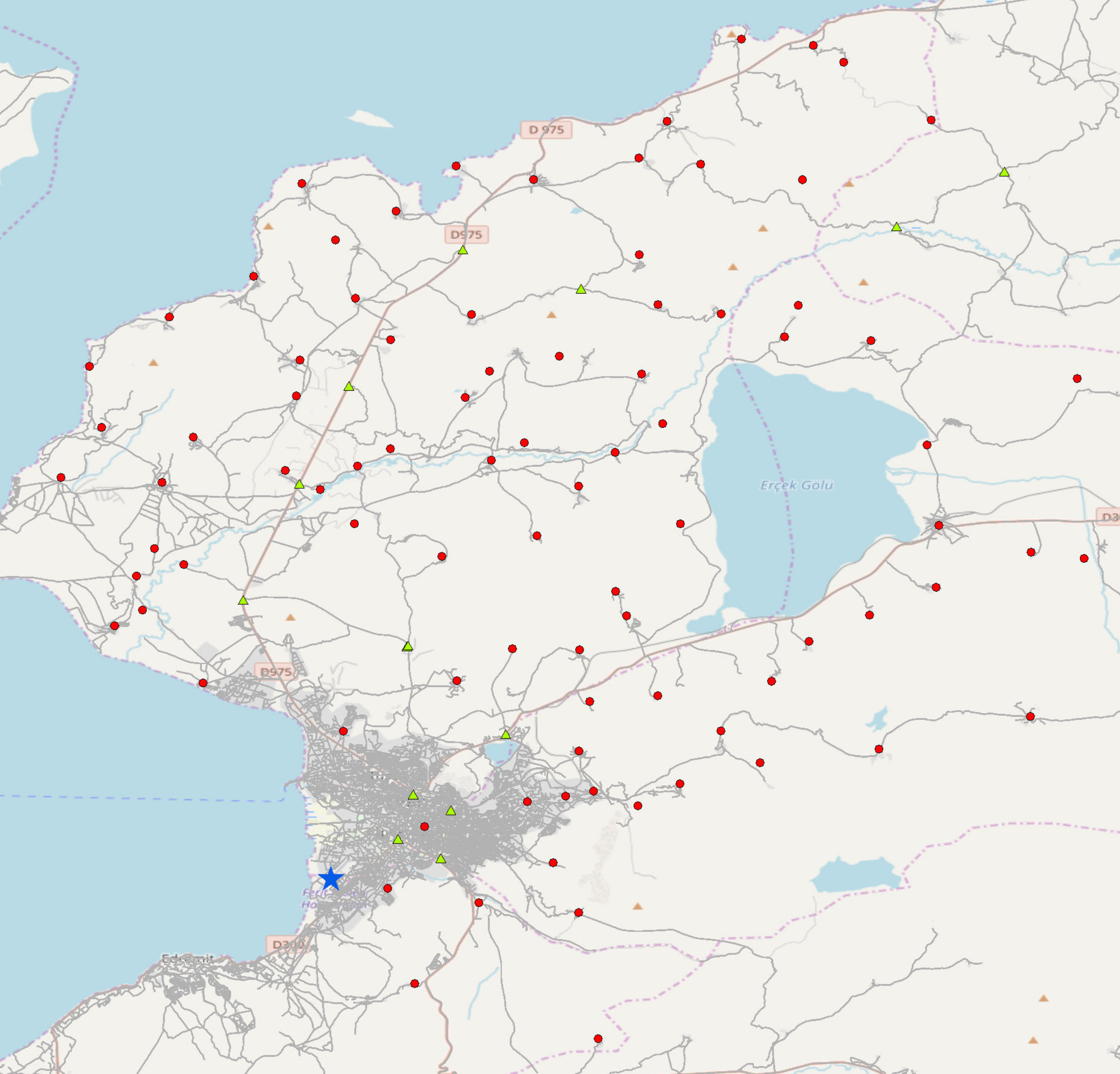
Turkey has experienced several severe earthquakes over the past few decades. One of the most destructive earthquakes struck eastern Turkey in Van province on October 23, 2011. The death toll rose to 600 people, while 4,100 individuals were injured. The 7.2 magnitude earthquake and its aftershocks left approximately 60,000 people homeless. One month after the event, about 120,000 people continued to receive warm food daily from the Van Food Assistance Center (Mehdi and Nazmazar (2013)). Fig. 3 shows the map of Van province, including the locations of demand nodes and junction points, as well as the depot. For more details about this case and how we prepared data for our analysis, refer to the Online Supplement.

Next, we present and analyze the computational results for the 60 instances derived from the Van province data set. We categorize the instances into four types based on vehicle capacity and maximum route length constraints. Type $A$ instances have abundant vehicle capacity and regular maximum route length. Type $T$ and $VT$ instances feature regular maximum route lengths, with tight and very tight vehicle capacities, respectively. Type $VTL$ instances exhibit both very tight vehicle capacity and maximum route length constraints. In these experiments, we set the value of $\epsilon$ to $0.85\,m\cdot\Psi$, recalling that $\Psi$ represents the maximum tour length and $m$ is the number of available vehicles.

Table 4 summarizes computational results for the Van earthquake case study, comparing the VF model solved with Gurobi to our B&P algorithm across various instance types, with metrics averaged by instance type. The Gap% column shows the optimality gap, and Time lists computational time in seconds for both methods. For the B&P algorithm, we include # Nodes (nodes explored), Avg. Columns (average columns per node), and the total columns generated by the MIP and GRASP methods for the pricing problem, labeled as # Columns MIP and # Columns GRASP. The LB-Gap% column indicates the percentage gap between lower bounds from Gurobi and B&P, with positive values showing B&P achieved a superior bound. The detailed computational results are reported in the Online Supplement.

As evident from Table 4, the B&P algorithm consistently finds a better or equal lower bound than the MIP solver across all instances. On average, the B&P algorithm provides a 1.347%, 1.185%, and 1.427% better lower bound for instances with 15, 30, and 60 nodes, respectively. Although the MIP solver may converge to the optimal solution faster than the B&P algorithm in “easy” instances (i.e., instances of types A and T), the B&P algorithm outperforms the MIP solver in all challenging instances (i.e., instances of types VT and VTL) in terms of execution time and optimality gap.

Table 4: Summary of computational results from the Van earthquake case study

Instance type	Model		B&P						LB-Gap%
	Gap%	Time	Gap%	Time	# Nodes	Avg. Columns	# Columns MIP	# Columns GRASP
Van15_A	0.000	0.6	0.001	13.7	1	84	42	39	0.000
Van15_T	0.005	0.5	0.000	14.3	1	102	44	56	0.001
Van15_VT	2.699	7200.4	0.007	54.9	4	310	136	274	2.698
Van15_VTL	2.691	7200.1	0.006	109.3	7	245	222	325	2.690
Van30_A	0.000	2.1	0.004	388.4	1	178	71	102	0.000
Van30_T	0.004	3.4	0.004	305.3	1	285	82	198	0.001
Van30_VT	2.395	7201.0	0.011	6273.6	15	912	430	1524	2.369
Van30_VTL	2.394	7201.0	0.011	6064.8	18	455	276	1003	2.371
Van60_A	0.000	27.7	0.008	3403.8	8	529	233	424	0.000
Van60_T	0.018	3691.7	0.005	1195.3	1	573	111	454	0.001
Van60_VT	1.733	7202.1	0.014	7229.9	3	4107	8	4470	1.639
Van60_VTL	4.292	7201.6	0.011	3709.5	10	841	19	1327	4.066
Average	1.352	3911.0	0.007	2396.9	6	718	139	849	1.320

Solving instances of types VT and VTL proves to be highly challenging, with the MIP solver unable to converge to the optimal solution within the 2-hour time limit for any of these instances. In contrast, the B&P algorithm finds high-quality solutions for all these instances, with an average gap of only 0.01%. For all 60 tested instances, our proposed algorithm either provides an optimal solution and verifies its optimality or finds a very high-quality solution with an average gap of 0.007% within the specified time limit.

From our computational results, it is evident that as the problem becomes more restrictive, regardless of its size, the optimality gap reported by the MIP-solver drastically increases. In contrast, the optimality gap for the B&P algorithm remains relatively stable. Remarkably, despite the B&P algorithm’s shorter runtime, its relative gap is consistently smaller than the one reported by the model, particularly for challenging instances.

In summary, our computational results on the Van data set suggest that the B&P algorithm is distinctly more efficient than solving the VF model by a MIP-solver. It can provide the optimal solution or a very high-quality solution in a reasonable time. Therefore, the proposed B&P algorithm is reliable to be utilized for decision making in post-disaster situations when both time and solution quality are of the utmost importance.

Figure 3: Map of Van province: the demand nodes are represented by red dots, the road junction points by green triangles, and the depot by a blue star.

5.2 Istanbul-Kartal real data

In this section, we test our approach on the data of the Kartal district of Istanbul provided by Kılcı et al. (2015), which were also used in Mostajabdaveh et al. (2019) for a location-allocation problem rather than a routing problem. As illustrated in Fig. 4, we adopt the twelve shelter locations proposed by Mostajabdaveh et al. (2019) and select a depot location based on the actual location of a relief supply distribution center in the region. We assume that $m=3$ identical vehicles are available for distributing relief supplies among the shelter locations. Additionally, we have fixed the value of $\epsilon$ to $0.85m\cdot\Psi$. For more information about the data preparation process, please refer to the Online Supplement.

Figure 4: Map of Istanbul’s Kartal district highlighting selected shelter locations (marked in green) and the central relief aid distribution center (marked in yellow).

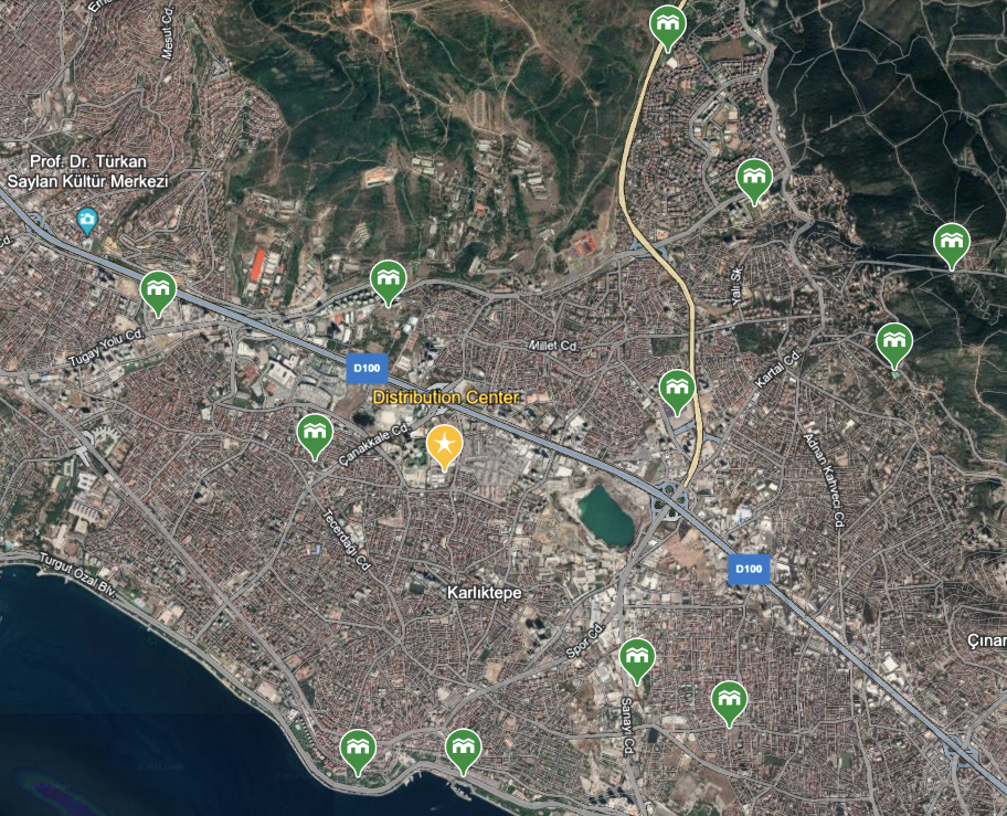
Table 5 summarizes our computational results for the Kartal case study, comparing the performance of the VF model solved with Gurobi and our B&P algorithm across various instance types. The meaning of the columns is the same as in Table 4. We report the detailed computational results in the Online Supplement.

Table 5: Summary of computational results for the Kartal case study

Instance type	Model		B&P						LB-Gap%
	Gap%	Time	Gap%	Time	# Nodes	Avg. Columns	# Columns MIP	# Columns GRASP
Kartal_A	0.000	0.2	0.004	250.6	68	90	661	496	-0.003
Kartal_T	5.148	7200.0	0.003	931.6	308	291	2310	2128	5.566
Kartal_VT	3.834	7200.0	0.005	915.8	341	230	2116	1958	4.055
Kartal_VTL	5.179	7200.0	0.007	783.0	70	140	790	512	5.563
Average	3.540	5400.1	0.005	720.3	197	188	1469	1274	3.795

In these instances, the average optimality gap obtained by the B&P algorithm turned out to be only about 1/775 of the average gap reported by the VF model solver, which is especially significant in view of the much shorter runtime of B&P (only 11/100), compared to the model solver. Remarkably, the B&P algorithm reaches the desired optimality gap in all 40 instances except one. Contrary to that, the model solver acts unpredictably, obtaining gaps of largely varying size, and only converges to the desired gap in type A instances. This confirms the superiority of the B&P approach again.

5.3 Contributions of the algorithmic components

Our B&P algorithm benefits from several enhancements, including an initial column generation heuristic, GRASP heuristics for the pricing problem, and valid inequalities for the mathematical pricing model. To evaluate the impact of these components on the performance of our B&P algorithm, we conducted a comprehensive analysis by introducing three distinct variations: (i) B&P without GRASP, (ii) B&P without valid inequalities, and (iii) B&P without initial route enhancements via Tabu Search. For this experiment, we utilized challenging instances from the Van earthquake dataset. Our findings indicate that the inclusion of Tabu Search for initial column enhancement is essential for achieving superior algorithm performance, as omitting it results in a 54.4% increase in runtime and gaps that are 59 times larger. Similarly, excluding valid inequalities in the pricing model leads to a 9.3% longer runtime and a 12.5% increase in the average gap. In contrast, while the GRASP algorithm improves efficiency for small and medium-sized instances, its effectiveness diminishes for larger problem instances. For a detailed exposition of our methodology, experimental setup, and an in-depth discussion of the results, we invite readers to consult the online supplement accompanying this paper.

5.4 Pareto front approximation

In this section, we aim to provide non-dominated Pareto solutions by changing the value of $\epsilon$ between $f^{max}_{2}$ and $f^{min}_{2}$. We obtain $f^{min}_{2}$ by solving the problem with minimization of the total traveling time as the objective. Similarly, $f^{max}_{2}$ is equal to the total traveling time of the optimal solution of the single objective problem with IAAF as the objective. To approximate the Pareto front, we solve a series of problem instances with varying $\epsilon$ values, starting from $f^{\max}_{2}$ and decrementing $\epsilon$ until reaching $f^{\min}_{2}$. At each step $t$, $\epsilon^{t}$ denotes the current $\epsilon$ value, and $f_{2}^{t}$ represents the second objective value of the optimal solution. Based on the augmented $\epsilon$-constraint method (Mavrotas and Florios, 2013) and our preliminary tests, we set the step size for decreasing $\epsilon$ to 1. We also apply the bypass mechanism from Mavrotas and Florios (2013), updating $\epsilon^{t}$ as $\min\{\epsilon^{t-1}-1,f_{2}^{t-1}-1\}$ to skip some $\epsilon$ values.

We select 20 instances with different characteristics from both case studies, including at least one instance from each instance type and size. We use the B&P algorithm or the MIP Solver to find the non-dominated solutions, selecting the approach that could find the optimal solution faster based on our experiments in the previous sections. We restrict the runtime for each instance of the auxiliary problem (i.e., the problem for a fixed $\epsilon$ value) to 600 seconds. Based on our preliminary experiments—presented in the Online Supplement—this time limit is sufficient for our solver to find solutions that are very close to optimal. Table 6 presents the results of these experiments. The first column lists the names of the instances. The subsequent columns report the selected solver, total number of instances solved, number of non-dominated solutions found, total runtime, $f^{max}_{2}$ and $f^{min}_{2}$, respectively.

Table 6: Pareto solutions

Instance	Solver	# Solved	# Non-dominated	Time	$f^{max}_{2}$	$f^{min}_{2}$
Van15_A1	MIP-Solver	8	4	1.3	41888	21692
Van15_T3	MIP-Solver	12	6	5.3	43766	21692
Van15_T5	MIP-Solver	8	6	2.2	39872	21694
Van15_VT5	B&P	16	7	458.5	44615	21696
Van15_VTL1	B&P	8	6	1218.5	30708	21696
Van30_A5	MIP-Solver	12	6	361.0	95335	32440
Van30_T1	MIP-Solver	24	15	829.9	83740	32524
Van30_T2	MIP-Solver	12	8	385.3	91901	32628
Van30_VT5	B&P	26	23	8557.2	88200	32524
Van30_VTL3	B&P	29	27	7274.0	71425	32628
Van60_A2	MIP-Solver	5	2	124.8	158612	47336
Van60_T2	B&P	35	28	18527.8	179760	47349
Van60_T5	B&P	25	18	13023.6	142704	47349
Van60_VT1	B&P	91	53	44807.7	166134	47189
Van60_VTL1	B&P	107	61	53109.5	138648	47189
Kartal_A2	MIP-Solver	7	5	1.5	46794	16341
Kartal_T3	B&P	12	11	289.3	42577	17664
Kartal_T6	B&P	10	9	1957.7	38032	17236
Kartal_VT7	B&P	8	6	231.5	34268	17664
Kartal_VTL5	B&P	10	9	147.8	20406	16698

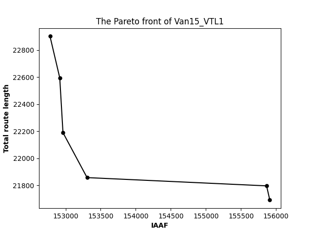
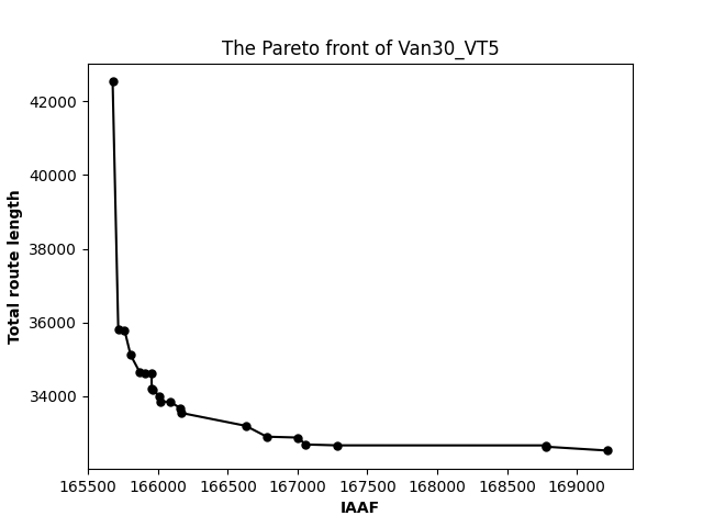
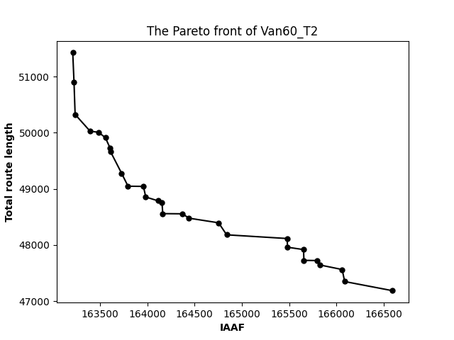
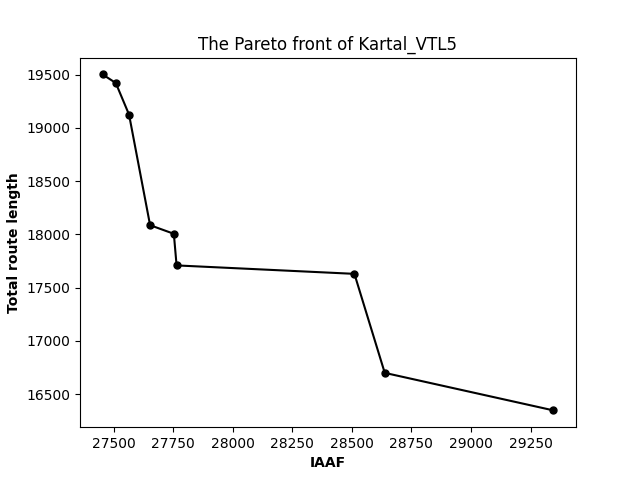
Although our step size to decrease $\epsilon$ was one, the total number of solved instances stayed relatively small, even for large instances. On average, 69% of the solved problem instances resulted in a non-dominated solution. In Figure 5, we approximate the Pareto fronts of four instances Van15_VTL1, Van30_VT5, Van60_T2 and Kartal_VTL5 by connecting the non-dominated solutions. The figures show the conflicting nature of the two objectives.

(a) Van15_VTL1 instance

(b) Van30_VT5 instance

(c) Van60_T2 instance

(d) Kartal_VTL5 instance

Figure 5: Pareto front of four selected instances

5.5 Price of Fairness

In this section, we analyze the consequences of decision-making processes that exclusively emphasize either fairness or efficiency and compare them to the use of the IAAF objective. The focus will be mainly on cases where the total traveling time is not restrictive. Three objectives will be investigated: (i) minimization of total unsatisfied demand: $\min D\mu=\min\sum_{i\in V_{c}}(d_{i}-v_{i})$, with solution MinUnD; (ii) minimization of Gini’s mean absolute difference multiplied by $D$: $\min D\Delta=\min\frac{1}{D}\sum_{i\in V_{c}}\sum_{j\in V_{c}}|d_{i}v_{j}-d_{j}v_{i}|$, with solution MinGini; and (iii) minimization of the IAAF objective multiplied by $D$: $\min D{\cal I}=\min D(\mu+\lambda\Delta)$, with solution MinIAAF. In addition to Gini’s mean absolute difference, we look at the Gini index ${\cal G}=\Delta/(2\mu)$. The parameter $\lambda$ is chosen as $\lambda=1/2$ (see Section 3).

We define the price of fairness (PoF) as the percentage increase in total unsatisfied demand caused by some “fair” solution (such as MinGini or MinIAAF), compared to perfect efficiency as achieved using the objective UnD, denoting total unsatisfied demand:

$$\mbox{PoF(MinGini)}=({\mbox{UnD(MinGini)}}/{\mbox{UnD(MinUnD)}}-1)\cdot 100$$

for MinGini, and analogously for MinIAAF. Fig. 6 presents the average price of fairness for each instance type when employing the solutions MinGini and MinIAAF, respectively. It turns out that the MinGini objective produces solutions with perfect equity (i.e., the Gini index equals zero) for all problem instances, and these perfectly equitable solutions exhibit an average 50% increase in total unsatisfied demand compared to the solutions with perfect efficiency. On the other hand, solutions obtained by using the IAAF objective turn out to be able to achieve perfect efficiency, resulting in a zero price of fairness. Still, they are not able to reduce the Gini index to zero, such that the MinGini solutions are superior to them in terms of fairness. Nevertheless, the MinIAAF solutions are equally efficient as those achieved by the MinUnD objective while simultaneously decreasing the Gini index by 33.68% relative to the UnD objective on average.

Figure 6: Evaluating percentage increases in Unsatisfied Demand for MinGini and MinIAAF objectives relative to the perfect efficiency (MinUnD Objective)

In summary, for scenarios without tight travel time constraints and with a moderate inequity-aversion parameter $\lambda$, we found that IAAF optimization produces lexicographically optimal solutions across all real-world test instances, prioritizing total demand coverage (primary objective) over minimizing Gini’s mean absolute difference (secondary objective), resulting in a PoF of zero. However, this is no longer the case when tighter total travel time limits are imposed; in this scenario, an essential trade-off between efficiency and fairness emerges.

The following table shows the PoF for the Kartal A2 test instance, varying according to ten values of the upper bound (UTTT) on total travel time:

$$\begin{array}[]{r|rrrrrrrrrr}\mbox{UTTT}&42635&21593&20560&20262&19661&19284&18775&17781&17702&17269\\ \hline\cr\mbox{PoF (\%)}&0&0&0&0&10.66&4.46&14.50&0&0&0\\ \end{array}$$

We can see that for intermediate bounds on the total traveling time, a nonzero price of fairness has to be taken into account. Of course, the range of scenarios where the price of fairness is larger than zero depends on the inequity aversion parameter $\lambda$: as $\lambda$ increases, indicating a higher ambition for fairness, the resulting PoF from the optimization model also grows.

It can be observed that prioritizing efficiency over fairness is advisable only when time constraints are either abundant or excessively restrictive. For practitioners, this suggests that in such conditions, lexicographic optimization with demand coverage as the more important criterion and distributional fairness as the second criterion may yield preferable plans —similar to those generated by our approach. However, if time constraints are moderately restrictive, this approach may prove insufficient. In such cases, a balanced consideration of coverage and fairness is essential to prevent significantly unfair plans.

6 Conclusion

We proposed a bi-objective optimization problem and an efficient algorithm for its exact solution to plan the allocation and distribution of scarce relief supplies via a fleet of vehicles to a set of shelters, originating from a single depot, in disaster response. Unlike previous studies, we optimized both an objective function measuring effectiveness and another accounting for fair supply allocation. To assess fairness, we utilized the widely recognized Gini coefficient. We focused on the early post-disaster stage, where insufficient supply at the depot makes full coverage unattainable within the specified time frame, necessitating the allocation of delivery amounts to each shelter.

We minimized both the total travel time of vehicles and an inequity-averse aggregation function (IAAF), which combines total unsatisfied demand with Gini’s absolute differences in unsatisfied demand. We established conditions for achieving perfect equity and derived key characteristics of the optimal solution with regard to the IAAF. Leveraging these insights, we proposed an algorithm that computes the optimal delivery amounts for given feasible vehicle routes using only simple arithmetic operators. Since a straightforward application of standard MIP solvers proved inefficient for tackling even the single-objective subproblems, we developed a branch-and-price (B&P) algorithm capable of handling real-world instance sizes. Our B&P method integrates several problem-specific enhancements, including route-deliveries as columns, a customized GRASP algorithm for the pricing problem, valid inequalities for the pricing problem, and an initial column generation heuristic based on the Tabu Search algorithm.

Our computational tests on realistic data from a past earthquake in Van, Turkey, and predicted data for the Kartal region of Istanbul, where a major earthquake is expected, demonstrate the superior performance of the B&P algorithm compared to commercial MIP solvers. Our bi-objective method can reduce the inequity of aid distribution by 34% without compromising efficiency. The results suggest that in cases where time constraints are either very loose or extremely tight, lexicographic optimization with demand coverage as the more important criterion and distributional fairness as the second criterion may yield good plans. However, if time constraints are moderately restrictive, a balanced approach is necessary to prevent inequitable outcomes.

Our problem setting currently restricts each demand point to a single-vehicle service, omitting potential efficiency gains from split deliveries, which could also enhance supply reliability through visit redundancy. Extending the problem to incorporate split deliveries is a promising avenue for future research. Additionally, exploring alternative frameworks for inequity aversion in optimization, such as the one presented in Chen and Hooker (2022), would be valuable. Finally, alternative mathematical formulations of the problem could be explored. We conducted preliminary experiments with alternative models based on the two-commodity flow formulation by Baldacci et al. (2004) and the multi-commodity formulation by Letchford and Salazar-González (2015). However, MIP solvers demonstrated better convergence with the model presented in this study. A deeper analysis would be worthwhile in future research.

Acknowledgements. While working on most parts of the study, the first author was a Ph.D. candidate at the College of Engineering, Koç University, Istanbul, Turkey.

Online Supplement
A B&P Algorithm for Fast and Equitable Last-Mile Relief Aid Distribution

1 Proof of Lemma 1

Suppose $v=(v_{i})_{i\in V_{c}}$ is an optimal solution, and consider an arbitrary $k_{0}\in K$. We will show that after changing the values $v_{i}$ for all $i\in V_{k_{0}}$ to demand-proportional values $v_{i}^{*}$ with the same sum $\sum_{i\in V_{k_{0}}}v_{i}^{*}=\xi_{k_{0}}$, the solution remains feasible, and the objective function value does not increase, i.e., $v^{*}$ is optimal again. As one can apply this consideration consecutively to all $k_{0}\in K$, it will prove the assertion of the Lemma.

Without loss of generality, assume $k_{0}=1$. Define

$$v_{i}^{*}=\xi_{1}\cdot\frac{d_{i}}{D_{1}}\;\>(i\in V_{1}),\quad v_{i}^{*}=v_{i}\;\>(i\in V_{k},\>k\neq 1).$$

First, the feasibility of $v^{*}=(v_{i}^{*})$ has to be shown. The feasibility of $v=(v_{i})$ implies

$$0\leq\xi_{k}\leq D_{k}\;\>(k\in K),\quad\xi_{k}\leq Q\;\>(k\in K),\quad\sum_{k\in K}\xi_{k}\leq C,$$

and hence

$$v_{i}^{*}\geq 0\>\;(i\in V_{1}),\quad v_{i}^{*}\leq D_{1}\cdot\frac{d_{i}}{D_{1}}=d_{i}\>\;(i\in V_{1}),$$

as well as

$$\sum_{i\in V_{1}}v_{i}^{*}=\xi_{1}\cdot\frac{D_{1}}{D_{1}}=\xi_{1}\leq Q$$

and

$$\sum_{i\in V_{c}}v_{i}^{*}=\xi_{1}+\sum_{i\in V_{c}\setminus V_{1}}v_{i}=\xi_{1}+\sum_{k\neq 1}\xi_{k}=\sum_{k\in K}\xi_{k}\leq C.$$

Therefore $v^{*}$ is feasible. Now consider the objective function. The first term of

$$\sum\limits_{i\in V_{c}}(d_{i}-v_{i})+\frac{\lambda}{D}\sum\limits_{i\in V_{c}}\sum\limits_{j\in V_{c}}|d_{i}v_{j}-d_{j}v_{i}|$$

is identical for $v$ and $v^{*}$, since

$$\sum_{i\in V_{c}}v_{i}=\sum_{k\in K}\xi_{k}=\sum_{i\in V_{c}}v_{i}^{*}.$$

It remains to show that

$$\sum_{i\in V_{c}}\sum_{j\in V_{c}}|d_{i}\,v_{j}-d_{j}\,v_{i}|\geq\sum_{i\in V_{c}}\sum_{j\in V_{c}}|d_{i}\,v_{j}^{*}-d_{j}\,v_{i}^{*}|.$$ (1.1)

Set $\bar{V}_{1}=V_{c}\setminus V_{1}$, decompose the l.h.s. of (1.1) into three terms $A_{1}+A_{2}+A_{3}$ with

$$A_{1}=\sum_{i\in V_{1}}\sum_{j\in V_{1}}|d_{i}\,v_{j}-d_{j}\,v_{i}|,\quad A_{2}=2\cdot\sum_{i\in V_{1}}\sum_{j\in\bar{V}_{1}}|d_{i}\,v_{j}-d_{j}\,v_{i}|,\quad A_{3}=\sum_{i\in\bar{V}_{1}}\sum_{j\in\bar{V}_{1}}|d_{i}\,v_{j}-d_{j}\,v_{i}|,$$

and decompose the r.h.s. of (1.1) into analogously defined terms $A_{1}^{*}+A_{2}^{*}+A_{3}^{*}$, replacing $v_{i}$ by $v_{i}^{*}$ $(i\in V_{c})$. Because of $v_{i}=v_{i}^{*}$ for $i\in\bar{V}_{1}$, it is obvious that $A_{3}=A_{3}^{*}$. Furthermore,

$$A_{1}^{*}=\sum_{i\in V_{1}}\sum_{j\in V_{1}}|d_{i}\cdot\xi_{1}\cdot\frac{d_{j}}{D_{1}}-d_{j}\cdot\xi_{1}\cdot\frac{d_{i}}{D_{1}}|=0,$$

so $A_{1}\geq A_{1}^{*}$. It remains to show that $A_{2}\geq A_{2}^{*}$, i.e., that

$$\sum_{i\in V_{1}}\sum_{j\in\bar{V}_{1}}|d_{i}\,v_{j}-d_{j}\,v_{i}|\geq\sum_{i\in V_{1}}\sum_{j\in\bar{V}_{1}}|d_{i}\,v_{j}-d_{j}\,v_{i}^{*}|$$ (1.2)

(note that $v_{j}^{*}=v_{j}$ for $j\in\bar{V}_{1}$). It suffices to show that for each fixed $j\in\bar{V}_{1}$, the inequality

$$\sum_{i\in V_{1}}|d_{i}\,v_{j}-d_{j}\,v_{i}|\geq\sum_{i\in V_{1}}|d_{i}\,v_{j}-d_{j}\,v_{i}^{*}|$$ (1.3)

holds. Division of (1.3) by $d_{j}$ and setting $\delta_{i,j}=d_{i}\cdot\frac{v_{j}}{d_{j}}$ transforms (1.3) into the equivalent representation

$$\sum_{i\in V_{1}}|\delta_{i,j}-v_{i}|\geq\sum_{i\in V_{1}}|\delta_{i,j}-v_{i}^{*}|.$$ (1.4)

For all $i\in V_{1}$,

$$\frac{v_{i}^{*}}{\delta_{i,j}}=\xi_{1}\,\frac{d_{i}}{D_{1}}\cdot\frac{d_{j}}{d_{i}\,v_{j}}=\xi_{1}\,\frac{d_{j}}{D_{1}\,v_{j}}=\xi_{1}/\sum_{s\in V_{1}}\delta_{s,j},$$

an expression which is actually independent of $i$. Substituting for $v_{i}^{*}$ by means of the last equation, we get

$$\sum_{i\in V_{1}}|\delta_{i,j}-v_{i}^{*}|=\sum_{i\in V_{1}}\left|\delta_{i,j}-\delta_{i,j}\cdot\frac{\xi_{1}}{\sum_{s\in V_{1}}\delta_{s,j}}\right|=\sum_{i\in V_{1}}\delta_{i,j}\left|1-\frac{\xi_{1}}{\sum_{s\in V_{1}}\delta_{s,j}}\right|$$

$$=\left|1-\frac{\xi_{1}}{\sum_{s\in V_{1}}\delta_{s,j}}\right|\>\left(\sum_{i\in V_{1}}\delta_{i,j}\right)=\left|\sum_{i\in V_{1}}\delta_{i,j}-\xi_{1}\right|=\left|\sum_{i\in V_{1}}(\delta_{i,j}-v_{i})\right|\leq\sum_{i\in V_{1}}|\delta_{i,j}-v_{i}|.$$

Thus (1.4) is shown, and the proof is complete.

2 Proof of Proposition 1

For each $k$, by the assumption $D_{k}/D\leq Q/C$, solution $\xi=(\xi_{k})$ given by

$$\xi_{k}=\frac{C}{D}\cdot D_{k}\quad(k\in K)$$

satisfies $\xi_{k}=C\cdot(D_{k}/D)\leq Q$, and because of $C\leq D$, also $\xi_{k}\leq D_{k}$ holds. Moreover, $\sum_{k\in K}\xi_{k}=C\leq C$. Together this shows that $\xi$ is feasible w.r.t. the constraint

$$0\leq\xi_{k}\leq\min(Q,D_{k})\;\>\forall k,\quad\sum_{k\in K}\xi_{k}\leq C.$$

Furthermore, $\xi$ clearly minimizes the part $D-\sum_{k}\xi_{k}$ of the objective function

$$D-\sum_{k}\xi_{k}+\frac{\lambda}{D}\,\sum_{k\in K}\sum_{\ell\in K}|D_{\ell}\xi_{k}-D_{k}\xi_{\ell}|$$ (2.1)

and the second part $\frac{\lambda}{D}\,\sum_{k\in K}\sum_{\ell\in K}|D_{\ell}\xi_{k}-D_{k}\xi_{\ell}|$ of this objective function becomes zero, which is minimal as well. This completes the proof.

3 Proof of Proposition 2

Without loss of generality, suppose that the condition $\frac{D_{k}}{D}>\frac{Q}{C}$ is satisfied for $k=1$, i.e., $\frac{D_{1}}{D}>\frac{Q}{C}$. Let $\xi$ be an optimal solution of (22) - (23), presented in the main text. Assume that the statement of the proposition is false, i.e., $\xi_{1}<Q$. We show that a contradiction follows.

First of all, it is shown that $\xi_{1}<C$: Suppose $\xi_{1}=C$. Then, since $\sum_{k\in K}\xi_{k}\leq C$, it follows that $\xi_{k}=0$ for all $k>1$, so we are dealing with the solution $\xi=(C,0,\ldots,0)$. Define $\xi^{\prime}=(\epsilon,C-\epsilon,0,\ldots,0)$. For sufficiently small $\epsilon>0$, solution $\xi^{\prime}$ is feasible again, and it is better than solution $\xi$: With $\bar{D}=\sum_{\ell>2}D_{\ell}$,

$$\psi(\xi^{\prime})=D-C+\frac{2\lambda}{D}\cdot\left\{|D_{1}(C-\epsilon)-D_{2}\epsilon|+\sum_{\ell>2}|D_{\ell}\,\epsilon|+\sum_{\ell>2}|D_{\ell}(C-\epsilon)|\right\}$$

$$=D-C+\frac{2\lambda}{D}\,[(D_{1}+\bar{D})C-(D_{1}+D_{2})\epsilon],$$

which is strictly decreasing with growing $\epsilon$, so $\psi(\xi^{\prime})<\psi(\xi)$ in contradiction to the optimality of $\xi$. This shows $\xi_{1}<C$. Distinguish now two cases:

Case (i): $\sum_{k\in K}\xi_{k}<C$ (total delivery amount is less than the total supply). Set $\xi^{\prime}=(\xi_{1}+\epsilon,\xi_{2},\xi_{3},\ldots,\xi_{m})$. Because of $\xi_{1}<C$, this is a feasible solution, provided that $\epsilon>0$ is sufficiently small, and that $\xi_{1}$ is not already identical to the upper bound $\min(Q,D_{1})$. However, the latter can be excluded: because of $\xi_{1}<Q$ by assumption, $\xi_{1}=\min(Q,D_{1})$ could only be the case if $\min(Q,D_{1})=D_{1}$ and hence $D_{1}\leq Q$. By ${D_{1}}/{D}>{Q}/{C}$, however, we have $D_{1}>(D/C)\,Q\geq Q$. So $\xi^{\prime}$ is feasible for small $\epsilon$.

We use the following general property (expressed in costs rather than benefits) of the Gini-based social welfare function ${\cal I}$ adopted in this paper: Suppose that ${\cal I}$ is applied to the costs $c_{i}$ of individuals $i\in I=\{1,\ldots,N\}$, and consider two cost vectors $c=(c_{1},\ldots,c_{N})$ and $c^{\prime}=(c^{\prime}_{1},\ldots,c^{\prime}_{N})$ with $c_{i}=c^{\prime}_{i}$ $(i\neq i_{0})$ and $c_{i_{0}}<c^{\prime}_{i_{0}}$. Then ${\cal I}[c^{\prime}]$ is strictly smaller (i.e., better) than ${\cal I}[c]$.

Note that strict monotonicity is asserted here, which requires a justification. As an OWA, measure ${\cal I}$ can be represented in the form ${\cal I}[c]=\sum_{i=1}^{N}q_{i}\,c^{(i)}$, where $c^{(1)}\leq c^{(2)}\leq\ldots\leq c^{(N)}$ is the sequence of cost values $c_{i}$ sorted in non-descending order, and the weights $q_{1}\leq q_{2}\leq\ldots\leq q_{N}$ are non-descending constants specific to the OWA function. For our generalized Gini measure,

$$q_{i}=\frac{2}{N^{2}}\left\{\frac{N}{2}+\lambda(2i-N-1)\right\}\quad(i=1,\ldots,N)$$

(see the Online Supplement to Mostajabdaveh et al. (2019)). It is easy to see that if $q_{i}>0$ for all $i$, then the claimed strict monotonicity property holds. Now, for $0\leq\lambda\leq 1/2$,

$$q_{1}=\frac{1}{N}-2\lambda\cdot\frac{N-1}{N^{2}}=\frac{1}{N}\,(1-2\lambda+\frac{2\lambda}{N})\geq\frac{2\lambda}{N^{2}}>0,$$

and hence also $q_{i}>0$ for all $i$.

Applied to benefits $v_{i}$ instead of costs $c_{i}=d_{i}-v_{i}$, the above result says that if the benefit of some individual is increased, leaving the benefits of the other individuals unchanged, then the evaluation by ${\cal I}$ is strictly improved (i.e., decreased). Successive application to each individual in $V_{1}$ immediately yields $\psi(\xi^{\prime})<\psi(\xi)$, in contradiction to the optimality of $\xi$.

Case (ii): $\sum_{k\in K}\xi_{k}=C$ (total delivery amount is equal to the total supply). Since $\xi_{1}<C$, there must be some $k\in K\setminus\{1\}$ for which $\xi_{k}>0$. We choose that $k\in K\setminus\{1\}$ for which ${\xi_{k}}/{D_{k}}$ is maximal; in other words, we look for the “best off” area $V_{k}$ for which the delivered supply per individual is at a maximum. Without loss of generality, assume that the route with maximal delivery-to-demand ratio is $k=2$. Set $\xi^{\prime}=(\xi_{1}+\epsilon,\xi_{2}-\epsilon,\xi_{3},\xi_{4},\ldots,\xi_{m})$. For $\epsilon$ sufficiently small, it is ensured that the solution $\xi^{\prime}$ is feasible; this would only be wrong if we would have $\xi_{1}=\min(Q,D_{1})$, such that $\xi_{1}$ could not be increased anymore. However, $\xi_{1}=\min(Q,D_{1})$ can be excluded as in case (i) above. So, again, $\xi^{\prime}$ is feasible for small $\epsilon$.

Observe now that ${\xi_{1}/}{D_{1}}<{\xi_{2}}/{D_{2}}$: Suppose this would not be true. Then from ${\xi_{1}}/{D_{1}}\geq{\xi_{2}}/{D_{2}}$, even ${\xi_{1}}/{D_{1}}\geq{\xi_{k}}/{D_{k}}$ for all $k$ would follow. However, because of ${D_{1}}/{D}>{Q}/{C}$, this would entail

$$\frac{\xi_{k}}{D_{k}}\leq\frac{\xi_{1}}{D_{1}}<\frac{Q}{D_{1}}<\frac{C}{D}\quad\forall k\in K,$$

and therefore

$$\xi_{k}<\frac{C}{D}\,D_{k}\quad\forall k\in K,\quad\sum_{k\in K}\xi_{k}<\frac{C}{D}\cdot D=C,$$

in contradiction to the assumption of case (ii).

Now, we apply the Pigou-Dalton Principle of Transfers (PDPT) (Moulin (2004)). It states that for a proper inequity-averse evaluation function, a transfer of a sufficiently small amount $e>0$ from a richer individual to a poorer individual results in a strict improvement of the inequity-averse evaluation function (cf. Weymark (2003), Fleurbaey and others (2006)). Because of $\xi_{2}/D_{2}>\xi_{1}/D_{1}$, the individuals in $V_{2}$ are richer than those in $V_{1}$. The generalized Gini function used by us satisfies the PDPT. Therefore, the transfer of the quantity $\epsilon$ from $V_{2}$ to $V_{1}$ improves the objective function, i.e., $\psi(\xi^{\prime})<\psi(\xi)$, so $\xi$ cannot be optimal in case (ii) either. This completes the proof.

4 Proof of Corollary 1

According to Prop. 2, if $\frac{D_{k}}{D}\geq\frac{Q}{C}$ then $\xi_{k}=Q$ and $\frac{C}{D}D_{k}\leq\xi_{k}\leq D_{k}$ does not hold. In case $\frac{D_{k}}{D}<\frac{Q}{C}$, according to Algorithm A.1, $\xi_{k}$ will be equal to $\frac{C}{D}D_{k}$ or $\frac{C^{\prime}}{D^{\prime}}D_{k}$. We can observe that any value of $\frac{C^{\prime}}{D^{\prime}}$ calculated during the algorithm is larger than $\frac{C}{D}$. This shows the assertion.

5 Multi-objective approach

We use the augmented $\epsilon$-constraint method by Mavrotas and Florios (2013), which augments the main objective function by subtracting the normalized slack variable of the added constraint. The augmented $\epsilon$-constraint method transforms the problem to

$$\min\{f_{1}(x)-\gamma\cdot\frac{s}{\theta}:\>f_{2}(x)+s=\epsilon,\>x\in{\cal X}\}$$ (5.1)

where $\gamma$ is a small machine precision constant, $\theta=f^{max}_{2}-f^{min}_{2}$ is the range of $f_{2}(x)$ values, and $s\geq 0$ is a nonnegative slack.

To adopt this approach, we choose our inequity measure as the main objective function and use the total traveling time objective for the $\epsilon$-constraint, i.e., we interchange the two objective functions in the main text, Subsection 3.1, such that now $f_{1}=z_{2}$ and $f_{2}=z_{1}$. The reason for the interchange is that it is computationally easier to handle the more complicated fairness-related objective function under formally simple constraints than, vice versa, a formally simple objective function under more complicated constraints. Note that this has only computational relevance and does not have any impact on the mutual rank of the two objective functions.

The optimal (i.e., minimal) value of the problem considering only the total travelling time objective yields $f^{min}_{2}$. To save runtime, we combine the augmented $\epsilon$-constraint method with the adaptive $\epsilon$-constraint approach: We start with the computation of the minimal solution $x^{*}_{1}$ of the problem with $f_{1}$ as the objective function and set $f^{max}_{2}$ and $\epsilon$ equal to $f_{2}(x^{*}_{1})$. To find the Pareto front, we then iteratively decrease the value of $\epsilon$ from $f^{max}_{2}$ to $f^{min}_{2}$. At each iteration, we solve the model (5.1) with a fixed bound $\epsilon$ to obtain the optimal solution $\hat{x}_{1}$, and set then $\epsilon$ equal to $f_{2}(\hat{x}_{1})-\delta$, where $\delta$ is a small step size, ensuring in this way that the previous solution is excluded.

6 Mathematical model of the pricing problem

Let us define the dual variables $\pi_{i,j}^{1}$, $\pi^{2}$, $\pi_{i}^{3}$, $\pi^{4}$ and $\pi^{5}$ corresponding to the constraints (28), (29), (30), (31) and (32) in the main paper, respectively. The reduced cost for variable $y_{r}$ can be calculated as follows:

$$c_{r}=-\sum_{i\in V_{c}}\sum_{j\in V_{c}}{(d_{j}q_{i}^{r}-d_{i}q_{j}^{r})\pi^{1}_{i,j}}-t^{r}\pi^{2}-\sum_{i\in V_{c}}a_{ir}\pi_{i}^{3}-\pi^{4}-\sum_{i\in V}(\pi^{5}+1)q_{i}^{r}+\frac{\gamma}{\theta}t^{r}.$$

The following variables describe a solution to the pricing problem: The binary variable $x_{i,j}$ attains the value one if and only if edge $(i,j)$ is used by the vehicle. The binary variable $a_{i}$ indicates whether demand point $i$ is visited by the vehicle or not, and $q_{i}$ is the amount of delivery to the node $i$. The mathematical formulation of the subproblem is presented below.

$$\min\> -\sum_{i\in V_{c}}\sum_{j\in V_{c}}{\bar{\pi}^{1}_{i,j}(d_{j}q_{i}-d_{i}q_{j})}-\sum_{(i,j)\in A}(\bar{\pi}^{2}-\frac{\gamma}{\theta})t_{i,j}x_{i,j}-\sum_{i\in V_{c}}\bar{\pi}^{3}_{i}a_{i}-\bar{\pi}^{4}-\sum_{i\in V_{c}}(\bar{\pi}^{5}+1)q_{i}$$ (6.1)

s.t. $$\sum_{(i,j)\in A}t_{i,j}x_{i,j}\leq\Psi$$ (6.2)

$$\sum_{i\in V_{c}}x_{0,i}=1$$ (6.3)

$$\sum_{i\in V_{c}}x_{i,n+1}=1$$ (6.4)

$$\sum_{j\in V_{c}}x_{i,j}-\sum_{j\in V_{c}}x_{j,i}=0,\qquad\forall i\in V_{c}$$ (6.5)

$$\sum_{j\in V_{c}}x_{i,j}=a_{i}\qquad\forall i\in V_{c}$$ (6.6)

$$\sum_{i\in S,j\in S}x_{i,j}\leq\sum_{i\in S,i\neq k}a_{i},\qquad\forall S\subset V_{c},\forall k\in S$$ (6.7)

$$q_{i}\leq d_{i}a_{i},\qquad\forall i\in V_{c}$$ (6.8)

$$\sum_{i\in V_{c}}q_{i}\leq Q$$ (6.9)

$$x_{i,j}\in\{0,1\},\quad\forall i,j\in V_{c}$$

$$a_{i}\in\{0,1\},\quad\forall i\in V_{c}$$

$$q_{i}\geq 0,\quad\forall i\in V_{c}$$ (6.10)

Objective function (6.1) is the reduced cost of a route-delivery (column) in RMP. Note that $\bar{\pi}_{i,j}^{1}$, $\bar{\pi}^{2}$, $\bar{\pi}_{i}^{3}$, $\bar{\pi}^{4}$ and $\bar{\pi}^{5}$ are constant values given by the dual solution of the RMP. Constraint (6.2) ensures that the route length does not exceed the specified maximum route length. Constraints (6.4) and (6.3) make sure that the route starts at the depot and ends at the depot. The balance between incoming and outgoing flow for each shelter is ensured by Eq. (6.5). Constraint (6.6) specifies the relation between $a_{i}$ and $x_{i,j}$ variables such that if node $i$ is not visited in the route, then all variables $x_{i,j},\,(j\in V_{c})$ should be zero. Subtour elimination is enforced by inequality (6.7) which is adopted from Feillet et al. (2005) for the TSP with profit problem. The delivery amount to node $i$ is limited by its demand $d_{i}$, which is guaranteed by constraint (6.8). Constraint (6.9) restricts the total delivery amounts in a route by the vehicle capacity.

7 Impact of total traveling time on equity

We select the solution of only minimizing the total traveling time as the reference solution. For each non-dominated solution, we calculate the percentage of total traveling time increase and IAAF decrease compared to the instance’s reference solution. To draw a general insight, we combine all data points obtained from instances of the same type, which produces the four plots presented in Fig 7.1. Points below the continuous line show the non-dominated solutions where the percentage of increase in total traveling time is smaller than the percentage of improvement in IAAF.

(a) Instances of type A

(b) Instances of type T

(c) Instances of type VT

(d) Instances of type VTL

Figure 7.1: Improvement of IAAF by increasing the total traveling time

In type A instances, IAAF is significantly improved by a slight increase in total traveling time. This does not hold in instances of type T but many points are below the straight line. On the contrary, for instances of types VT and VTL, most of the points are above the straight line (see Fig. 1(c) and Fig. 1(d)), which means that a larger amount of the total traveling time should be sacrificed. Finally, as the instances become more restricted regarding vehicle capacity and maximum route length, the improvement in IAAF becomes smaller and harder to achieve.

8 GRASP heuristic for the pricing problem

A solution to the pricing problem, and thus also the output of our GRASP algorithm, consists of two parts, a single vehicle route that visits a subset of nodes, and a vector of delivery quantities to the visited nodes. The constructive phase of our GRASP adaptation starts with sorting the nodes according to a score and selecting one node randomly from a truncated list RCL of nodes. Then a route that only visits the chosen node is created.

To create the node selection measure, we use a proxy on the contribution of nodes on the pricing problem objective function (B.1). Since we cannot decide on the $q_{i}$ variables before knowing which nodes are selected, we consider the objective value change for a unit increase in delivery quantity $q_{i}$ in our node score measure. Following this approach, we set $q_{i}=1,\,\forall i\in V_{c}$ and try to separate the pricing problem objective (B.1) for every node $i$. Note that the second term in the objective cannot be written for each node separately, thus we ignore it in our heuristic measure. The node scores are calculated as follows: $\sigma(i)=-\sum_{j\in V_{c}}\left(\bar{\pi}^{1}_{ij}-\bar{\pi}^{1}_{ji}\right)d_{j}-\bar{\pi}^{3}_{i}-(\bar{\pi}^{5}+1),\quad\forall i\in V_{c}$. The list RCL is created such that RCL$=\{i\,|\,\sigma(i)\leq\alpha\cdot\sigma^{min}\}$, where $\alpha$ is a parameter that controls the size of the list, and $\sigma^{min}$ is the minimum node score. The heuristic selects one node from RCL uniformly at random. Each possible insertion of a node is evaluated according to the reduced cost of the route-delivery (see below). The node will be inserted to the best position for which the insertion does not violate the vehicle route length constraint. To calculate the reduced cost of any insertion, we obtain the delivery amounts by using Algorithm 3.3. The heuristic updates the RCL list by removing the previously selected nodes and repeating the above steps. This is continued until none of the remaining nodes can be inserted feasibly into the route, or all of them have a non-negative value. As a result, we obtain an incumbent solution which will be improved in the second phase. Algorithm 3.1 shows the detailed steps of the constructive phase of our GRASP heuristic.

Algorithm 3.1 GRASP to solve pricing problem: Constructive phase

 Input: $V_{c}$, $\Psi$, Dual variables, $\sigma(i)$.

 Output: One route-delivery

 Create an empty route, $\bar{r}\leftarrow[0,n+1]$.

 while $any(\sigma(i)<0,\forall i\in I^{un})$ and $I^{un}\neq\emptyset$ do

  $RCL=\{i\in I^{un}|\sigma(i)\leq\alpha\times\sigma^{min}\}$.

  Select $\bar{i}$ randomly from RCL.

  $CL=\{\}$

  for p in [all possible insertion positions of $\bar{r}$] do

   Build route $r^{\prime}$ by inserting $\bar{i}$ into $\bar{r}$ at $p$.

   if length $r^{\prime}$ is less than or equal to $\Psi$ then

    Calculate delivery amounts for nodes served by $r^{\prime}$ with Algorithm 3.3.

    Calculate the reduced cost of the $r^{\prime}$, $RC(r^{\prime})$, and store in CL.

   end if

  end for

  if $CL\neq\emptyset$ then

   Find the route-delivery in CL with minimum reduced cost, $r^{\prime\prime}$.

   if $RC(r^{\prime\prime})\leq RC(r)$ then

    Replace $\bar{r}$ with $r^{\prime\prime}$.

   end if

  end if

  Remove $\bar{i}$ from $I^{un}$

 end while

 Return route delivery $\bar{r}$

In the second phase, we improve the incumbent solution by a Local Search procedure based on neighborhoods defined by two types of moves: Let us denote by $I^{un}$ the set of nodes that are not visited by the current route. The first move, Exchange, exchanges one node from $I^{un}$ with one node from the current vehicle route. The other move, Insertion, inserts one node from $I^{un}$ to the best possible position in the current route, given that the insertion is feasible regarding the maximum route length constraint. At each iteration, our heuristic explores all possible Exchange moves and accepts the one with the maximum improvement. With the updated incumbent solution, the heuristic evaluates all possible Insertion moves, accepts the best one, and moves on to the next iteration. We terminate the procedure when no further improvement can be found anymore. During the algorithm, we store every solution with a negative reduced cost and use these solutions as new columns in the column generation. The pseudocode of the improvement phase of our GRASP heuristic is presented by Algorithm 3.2.

Algorithm 3.2 GRASP to solve pricing problem: Improvement phase

 Input: $V_{c}$, $\Psi$, Dual variables, An initial route-delivery $\bar{r}$.

 Output: A set of route-deliveries with negative reduced cost $\bar{R}$.

 Define $I(\bar{r})$ as the set of nodes (except depot) visited by $\bar{r}$.

 while Improvements are found in previous iteration do

  $I^{un}=V_{c}\setminus I(\bar{r})$, $CL=\{\}$.

  for $i\in I^{un}$ do

   for $j\in I(\bar{r})$ do

    Build $r^{\prime}$ by replacing $i$ with $j$ in $\bar{r}$.

    if length $r^{\prime}$ is less than or equal to $\Psi$ then

     Calculate the reduced cost of $r^{\prime}$, $RC(r^{\prime})$, and store in CL if $RC(r^{\prime})\leq 0$.

    end if

   end for

  end for

  if $CL\neq\emptyset$ then

   $\bar{R}=\bar{R}\bigcup CL$.

   Replace $\bar{r}$ with the route-delivery with minimum reduced cost in CL.

  end if

  $I^{un}=V_{c}\setminus I(\bar{r})$, $CL=\{\}$.

  for $i\in I^{un}$ do

   for p in [all possible insertion positions of $\bar{r}$] do

    Build route $r^{\prime}$ by inserting $\bar{i}$ into $\bar{r}$ at $p$.

    if length $r^{\prime}$ is less than or equal to $\Psi$ then

     Calculate the reduced cost of $r^{\prime}$ $RC(r^{\prime})$, and store in CL if $RC(r^{\prime})\leq 0$.

    end if

   end for

  end for

  if $CL\neq\emptyset$ then

   $\bar{R}=\bar{R}\bigcup CL$.

   Replace $\bar{r}$ with the route-delivery with minimum reduced cost in CL.

  end if

 end while

 Return $\bar{R}$.

To evaluate a considered move during the GRASP heuristic, we decide first on the delivery quantities to each node visited by the route, which creates a route-delivery. Then we calculate the reduced cost associated with a move using the pricing problem objective function. We use a simple algorithm to calculate delivery amounts. The algorithm presented in Algorithm 3.3 is guaranteed to find the optimal delivery amounts in the pricing problem for a given route so that only the routing part is solved heuristically. Let us assume the vehicle route $\bar{r}$ is given, and $V_{\bar{r}}$ is the set of nodes that this route serves. Optimality of the deliveries with respect to the objective function (B.1) is seen as follows:

For a given route $\bar{r}$ that visits the nodes in $V_{\bar{r}}$, the pricing problem reduces to

$$\min\> -\sum_{i\in V_{c}}\sum_{j\in V_{c}}{\bar{\pi}^{1}_{i,j}(d_{j}q_{i}-d_{i}q_{j})}-(\bar{\pi}^{5}+1)\sum_{i\in V_{\bar{r}}}q_{i}$$ (8.1)

$$q_{j}=\frac{d_{j}}{d_{i}}q_{i},\quad\forall i\in V_{c},j\in V_{c}$$ (8.2)

$$\frac{C}{D}\sum_{i\in V_{\bar{r}}}d_{i}\leq\sum_{i\in V_{\bar{r}}}q_{i}+Cz$$ (8.3)

$$\frac{C}{D}\sum_{i\in V_{\bar{r}}}d_{i}\leq Q+Cz$$ (8.4)

$$\sum_{i\in V_{\bar{r}}}q_{i}\geq Qz$$ (8.5)

$$\sum_{i\in V_{\bar{r}}}q_{i}\leq Q$$ (8.6)

$$0\leq q_{i}\leq d_{i},\quad\forall i\in V_{\bar{r}}$$ (8.7)

$$q_{i}=0,\quad\forall i\in V_{c}\setminus V_{\bar{r}}$$ (8.8)

The objective function can be rewritten as

$$-\sum_{i\in V_{\bar{r}}}\sum_{j\in V_{c}}{\bar{\pi}^{1}_{i,j}d_{j}q_{i}}+\sum_{i\in V_{c}}\sum_{j\in V_{\bar{r}}}\bar{\pi}^{1}_{i,j}d_{i}q_{j}-(\bar{\pi}^{5}+1)\sum_{i\in V_{\bar{r}}}q_{i}.$$

We denote $\kappa_{i}$ as the coefficient of variable $q_{\hat{i}}$ in the above objective which for a specific $\hat{i}\in V_{\bar{r}}$ computes as

$$\kappa_{\hat{i}}=-\sum_{j\in V_{c}}{\bar{\pi}^{1}_{\hat{i},j}d_{j}+\sum_{i\in V_{c}}\bar{\pi}^{1}_{i,\hat{i}}d_{i}-(\bar{\pi}^{5}+1)}=-(\bar{\pi}^{5}+1)-\sum_{j\in V_{c}}(\bar{\pi}^{1}_{\hat{i},j}-\bar{\pi}^{1}_{j,\hat{i}})d_{j},$$ (8.9)

Using equation (8.2) we can transform the problem (8.1)-(8.8) by substituting $q_{j}$, $j\in V_{\bar{r}}\setminus\{\hat{i}\}$ with $q_{\hat{i}}d_{j}/d_{\hat{i}}$. This turns the above optimization problem into a continuous optimization problem with one bounded variable. Variable $q_{\hat{i}}$ has its optimal value on its lower or upper bound. Thus, we can solve the problem to optimality by the greedy algorithm presented in Algorithm 3.3.

Algorithm 3.3 Algorithm to obtain the delivery amounts

 Input: A route-delivery $\bar{r}$, $d_{i}$, $\kappa_{i}$ (computed by (8.9)), $C$, $Q$.

 Output: Route-delivery $\bar{r}$ with new delivery amounts $q_{i},\forall i\in V_{\bar{r}}$.

 $D_{\bar{r}}=\sum_{i\in V_{\bar{r}}}d_{i}$.

 $\hat{i}=argmin\{d_{i}|i\in V_{\bar{r}}\}$.

 if $\frac{D_{\bar{r}}}{D}\geq\frac{Q}{C}$ then

  $q_{\hat{i}}=d_{\hat{i}}{Q}/{D_{\bar{r}}}$.

 else

  Calculate the coefficient of $q_{\hat{i}}$ in the objective function, $\hat{c}=\sum_{i\in V_{\bar{r}}}\kappa_{i}{d_{i}}/{d_{\hat{i}}}$.

  if $\hat{c}<0$ then

   $q_{\hat{i}}=\min\{d_{\hat{i}},d_{\hat{i}}{Q}/{D_{\bar{r}}}\}$.

  else

   $q_{\hat{i}}=d_{\hat{i}}{C}/{D}$.

  end if

 end if

 for other nodes i in $V_{\bar{r}}\setminus\{\hat{i}\}$ do

  $q_{i}=q_{\hat{i}}{d_{i}}/{d_{\hat{i}}}$

 end for

 Return route-delivery $\bar{r}$ with new delivery amounts $q_{i}$.

9 Tabu Search algorithm to create initial columns

The parallel variant of the CW algorithm starts with vehicle routes containing only the depot and one customer. Routes are merged to larger routes in a step-by-step manner. At each step, the cost savings of merging all pairs of routes are calculated, and a feasible merger with the highest savings is implemented. The algorithm is repeated until none of the remaining mergers is feasible. A merger is considered feasible only if the length of the resulting route is less than $\Psi$. We adapt the CW heuristic to create solutions with load-balanced routes. We abandon the vehicle capacity constraint and assume that route feasibility only depends on maximum route length. We adapted the CW algorithm to our problem by an extension of the saving cost computation: instead of considering only the changes in route lengths, we also take the effect of joining two routes on Gini’s mean absolute difference into account. For the sake of brevity, we omit the details.

We continue merging routes until we can not find any feasible merger, even if the saving has a negative value. Thus, the CW heuristic tries to minimize the number of vehicles. The CW heuristic always ensures the feasibility of the routes regarding the maximum length $\Psi$, but the number of created routes may by larger than $m$, or the total traveling time may exceed $\epsilon$. As the next step, we apply the Lin-Kernighan heuristic (see Lin and Kernighan (1973)), one of the most effective heuristics to solve the TSP, to each route in order to reduce the route length. We use a recent implementation of the algorithm, LKH-2.0.9, accessible at http://webhotel4.ruc.dk/ keld/research/LKH/. To create route-deliveries from the set of routes, we employ Algorithm A.1 to find the optimal delivery quantities.

Next, we develop a Tabu Search (TS) heuristic to improve the solution quality while retaining the solution feasibility. For many years, TS has remained among the most popular algorithms to solve VRPs, due to its efficiency, flexibility, and simplicity. Please refer to Osman (1993), Gendreau et al. (1994) and Toth and Vigo (2003) for successful TS designs. Tabu search is an iterative algorithm that starts with an initial solution $s$ and tries to find a better solution by moving to a neighbor solution in each iteration. The implemented moves are considered forbidden for a number of iterations to avoid returning to previous solutions.

We use the neighborhood definition that is generated by a Relocate move, which removes a node from a route and inserts it to the best possible position in another route. To restrict the number of possible moves and to accelerate the TS, we use heuristic punning (Toth and Vigo (2003)). First, for each node, we define the set of $n^{near}$ nearest neighbors and only insert a node before or after one of its neighbors. In every iteration, we randomly select a subset of $\eta$ nodes, using a uniform probability distribution, and evaluate all candidate moves. A move with the best fitness value will be accepted if it is not prohibited. We also use the Aspiration Criterion (Glover (1990)), meaning that we do accept a prohibited move if it improves the best solution found so far. The accepted move is then considered prohibited and will be kept in the tabu list for a certain number of iterations, randomly selected between $\omega_{min}$ and $\omega_{max}$. The algorithm continues until the number of consecutive iterations without improvement exceeds $it^{NO}$.

To evaluate the fitness of a new solution $s^{\prime}$, first, we decide on the delivery quantities to each node using Algorithm A.1. Denote by $r$ a route-delivery in set $RD(s^{\prime})$, where the latter is the set of all route-deliveries belonging to solution $s^{\prime}$. Then we calculate the fitness $F(s^{\prime})$ of solution $s^{\prime}$ as follows:

$$F(s^{\prime})=D\cdot{\cal I}(s^{\prime}) +\frac{\gamma}{\theta}\max(0,\sum_{r\in RD(s^{\prime})}t^{r}-\epsilon)$$

$$+\nu^{MLR}\sum_{r\in RD(s^{\prime})}\max(0,t^{r}-\Psi)+\nu^{NV}\max(0,|RD(s^{\prime})|-m)$$ (9.1)

The first two terms of the above fitness function are calculated according to the SP formulation’s objective function. The third and forth terms act as a penalty cost for a violation of the constraints on maximum route length and the number of available vehicles, respectively. The parameters $\nu^{MLR}$ and $\nu^{NV}$ are the penalty coefficients for these violations. These parameters have to be tuned before using the algorithm. Since the primary aim of our TS heuristic is to find a set of feasible solutions, we use large values for $\nu^{MLR}$ and $\nu^{NV}$.

Algorithm 4.1, which uses Algorithm A.1 as a subprocedure, presents the steps of our TS heuristic. In the description of Algorithm 4.1, we denote the best solution (e.g., a solution with the smallest fitness value) found so far by $s^{BS}$, and the best feasible solution by $s^{BFS}$. We define $s^{IN}$ as the incumbent solution and $\mathcal{S}^{CA}$ as the set of candidate solutions for the next incumbent solution; this set consists of neighbor solutions of $s^{IN}$ generated by the Relocate move. A move $(i,k)$ is defined by the node $i$ that is relocated from its current route to the best position in the destination route $k$, and by the index $k$ of the destination route. Algorithm 4.1 presents the pseudocode of our Tabu Search algorithm.

Algorithm 4.1 Tabu search algorithm

 Input: Algorithm parameters, Initial solution $s$.

 Output: A set of feasible solutions, $\mathcal{S}^{F}$

 $s^{BS},s^{IN}\leftarrow s$

 $it\leftarrow 0$

 $\mathcal{S}^{F}=\emptyset$

 while $it\leq it^{NO}$ do

  Create set $V^{S}$ which contains $\eta$ nodes randomly selected from $V_{c}$.

  for $i$ in $V^{S}$ do

   Determine set $V^{near}(i)$ as the set of $n^{near}$ nearest nodes to node $i$

   Define $K^{near}(i)$ as the set of routes visit at least one node in $V^{near}(i)$

   for route $k$ in $K^{near}(i)$ do

    Creating neighbor solution $s^{\prime}$

    Insert node $i$ in the best position in route $k$

    Calculate delivery quantities for the updated routes using Algorithm

    Calculate $F(s^{\prime})$

    if move ($i$,$k$) is not in Tabu list then

     Add $s^{\prime}$ to $\mathcal{S}^{CA}$ set

    else if $F(s^{\prime})<F(s^{BS})$ or ($s^{\prime}$ is feasible and $F(s^{\prime})<F(s^{BFS})$) then

     Add $s^{\prime}$ to $\mathcal{S}^{CA}$ set

    end if

   end for

  end for

  $s_{min}$ $\leftarrow$ the solution with minimum fitness in $\mathcal{S}^{CA}$

  if $F(s_{min})<F(s^{BS})$ then

   $s^{BS}\leftarrow s_{min}$

  end if

  $s^{F}_{min}$ $\leftarrow$ the feasible solution with minimum fitness in $\mathcal{S}^{CA}$

  if $F(s^{F}_{min})<F(s^{BFS})$ then

   $s^{BFS}\leftarrow s^{F}_{min}$

   $\mathcal{S}^{F}=\mathcal{S}^{F}\cup\{s^{BFS}\}$

  end if

  if $F(s_{min})\leq F(s^{IN})$ then

   $s^{IN}\leftarrow s_{min}$

   $it=0$

   Generate $\omega_{(i,k)}$ randomly between $\omega_{min}$ and $\omega_{max}$

   Keep the move ($i,k$) for $\omega_{(i,k)}$ in Tabu List.

  else

   $it=it+1$

  end if

  Remove the moves that stayed more than $\omega_{(i,k)}$ iterations in Tabu List.

 end while

For each feasible solution in $\mathcal{S}^{F}$, we run the LKH heuristic on each vehicle route separately as a post-optimization step. Table 9.1 lists the parameters of the algorithm together with their values as used in the experimental part.

Table 9.1: Parameters for the Tabu Search heuristic

Parameter	Description	Value
$\eta$	Number of nodes selected for relocation in each iteration	$\lceil\frac{n}{5}\rceil$
$n^{near}$	Number of nodes considered near to a node	$\lceil\frac{n}{3}\rceil$
$[\omega_{min},\omega_{max}]$	Bounds on the number of iterations     for which a move is prohibited	$[2,6]$
$it^{NO}$	Maximum number of consecutive iterations     without improvement before termination	20
$\nu^{MLR}$	Coefficient of maximum route length violation in fitness function	$10\max\limits_{(i,j)\in A}t_{i,j}$
$\nu^{NV}$	Coefficient of maximum number of vehicles violation in fitness function	$10\max\limits_{(i,j)\in A}t_{i,j}$

10 Van earthquake data preparation

As our first case study, we build on real-world data from the 2011 Van earthquake, made available to us by Noyan et al. (2015). We suitably adapted the data to our problem formulation in order to obtain test instances. There are 94 settlements that have been affected by the earthquake; one local distribution center was responsible for distributing the relief items immediately after the disaster. Noyan et al. (2015) studied a problem of deciding on the location of the relief aid distribution points (PODs) in a limited number of districts, on their capacity, on the allocation of supply to these distribution centers from the LDC, and on the assignment of demand points to PODs as a preparedness measure.

In our study, we focus on relief aid distribution in the post-disaster phase where the demands and the (possibly damaged) state of the road network are known. Therefore, instead of constructing different scenarios, we generate instances with different characteristics and solve our relief routing problem for each instance separately. To generate demands, we exactly follow the approach of Noyan et al. (2015). However, to generate realistic post-disaster distances between road network nodes, taking possible damages into account, we apply the network sampling algorithm described in Yücel et al. (2018), which has also been used in Mostajabdaveh et al. (2019) (see below). The network has 94 demand points which can also act as intermediate points for the routes, and one LDC, the depot where all prepositioned supply is stored. The vehicles start and end their routes at the depot. In addition to the 94 demand points, we added 14 road junction points and built graph $G=(V,E)$, where $V$ is the set of all nodes (junctions, demand points and LDC) and $E$ is the set of edges that connect nodes. We assume that there is a direct edge between every two nodes that have a distance less than 3 kilometres. The traveling times on the edges were calculated by the ArcGIS Pro $2.3.3$ software.

To consider post disaster road damage when generating distances, we use the link failure dependency model presented in Yücel et al. (2018). We partition the set of edges into three sets $E_{d}$, $E_{a}$, and $E_{s}$, according to the damage intensity category of their endpoints. The edges that have one or two endpoints with damage intensity destructive are placed in set $E_{d}$. From the remaining edges, those having one or two endpoints with intensity damaging are assigned to set $E_{a}$. Set $E_{s}$ contains the edges that do not belong to either of the two other sets. Each edge $e\in E$ has a survival probability of $p_{e}$, which is the probability that the edge remains intact after the disaster. For each of our sample instances, we assign the initial $p_{e}$ values to the edges in the sets $E_{d}$, $E_{a}$ and $E_{s}$ by uniformly selecting a random value from the interval $[0.7,0.8]$, $[0.8,0.9]$ and $[0.9,1]$, respectively. The link failure dependency model determines which edges are going to fail and which will remain functional in the post-disaster network, introducing local correlations between the failure events. We use this information to calculate the shortest paths between the demand nodes and the depot in the damaged post-disaster network.

In order to reduce the size of the problem, Noyan et al. (2015) clustered the demand nodes and created new networks with 15, 30, 60 nodes. The demand within each cluster is aggregated and assigned to a selected node inside the cluster, cluster centriod, which represents the cluster. Relief distribution in Noyan et al. (2015) was only considered in the form of distribution of the supply from the depot to selected PODs. However, here we consider the case where the supply has to be transported directly from the depot to the demand points. It is sufficient for practice to solve the problem only on the 15-, 30- and 60-node-networks instead of the original 94-node-network since the beneficiaries can reach the cluster centroids easily. We set the number of vehicles equal to 3, 5 and 9 for instances with 15, 30 and 60 shelters, respectively. To calculate the distances between two nodes in the reduced networks, we first generate the distances in the original network with 94 nodes according to the procedure described above. Then we only keep the edges that their endpoints are the clusters’ centroids.

In total, we generate 60 random instances, 20 for each of the problem sizes. We divide the number of nodes by the number of vehicles and multiply it by the average traveling time between any two nodes to obtain the maximum route length $\Psi$, such that $\Psi=\zeta^{1}\lceil n/m\rceil\cdot\bar{t}$ where $\bar{t}=\sum\limits^{n}_{i=1}\sum\limits^{n}_{j=1}t_{i,j}/n(n-1)$ and $\zeta^{1}$ is a coefficient that controls maximum route length.

For instances where we aim at generating a regular maximum route length, we set $\zeta^{1}=2$, while for instances with very tight maximum route length, we set $\zeta^{1}=1$. We assume that the total available supply at the depot is equal to 70 % of the total demand, i.e., $C=\zeta^{2}\sum_{i}d_{i}$ with $\zeta^{2}=0.7$. The capacity of a vehicle is calculated as $Q=\zeta^{3}\frac{C}{m}$ where for a tight, but not very tight capacity, we select $\zeta^{3}=0.5$, while for a very tight capacity, we set $\zeta^{3}=0.2$. The purpose of picking comparably tight capacities is to observe the performance of the algorithm under stress, considering that generous vehicle capacities make the problem computationally easy. However, for the sake of completeness, we generate a few instances with abundant vehicle capacity, where $\zeta^{3}=1.2$. Finally, the value $\epsilon$ is fixed to $0.85m\cdot\Psi$.

11 Detailed results of Van data set

Tables 11.1, 11.2 and 11.3 report the computational results obtained by executing both the MIP-solver for the VF model and the B&P algorithm on these instances. The first column in each of these tables shows the instance name. The first number in instances names indicates the number of shelters that are to be visited by the vehicles. The second number indicates the instance identifier within each group of instances. The letters after “_” in the instance name indicate the instance type. The next column presents the computational time for $\theta$ values using the column generation approach, as described in Section 5. The next four columns in Table 11.1 present the results obtained by solving the VF model with the MIP-solver. The first two columns, UB and LB, report the best feasible solution value and the lower bound found until termination, respectively. The column Time shows the execution time (in seconds) of the MIP solver. The percentage gap between the lower bound and the upper bound (i.e., the optimality gap) is reported in the column Gap. The next four columns under B$\&$P provide analogous information to the four columns for Model, but now refer to our B&P algorithm. For the B$\&$P algorithm, we also report the number of branch-and-bound tree nodes explored before termination under # Nodes, the average number of columns in the column set at each node under Avg. Columns, and the total number of columns with negative reduced cost generated by MIP and GRASP when solving the pricing problem. Finally, the last column, LB-Gap, represents the percentage gap between the lower bound reported by the model solver and that of the B$\&$P algorithm. Note that a positive value for LB-Gap indicates that the B$\&$P algorithm was able to find a better lower bound than the MIP solver.

Table 11.1: Van earthquake case study results on the 15 node-network with 3 vehicles

Instance	Time to $\theta$	Model				B&P								LB-Gap%
		UB	LB	Gap%	Time	UB	LB	Gap%	Time	# Nodes	Avg. Columns	MIP	GRASP
Van15_A1	17.8	111016.0	111015.3	0.000	0.7	111015.8	111015.7	0.000	14.0	1	77	44	30	0.000
Van15_A2	15.1	112810.6	112809.7	0.000	0.5	112812.1	112809.8	0.002	13.7	1	93	41	49	0.000
Van15_A3	17.7	101100.7	101100.0	0.000	0.3	101100.4	101100.4	0.000	13.9	1	89	42	44	0.000
Van15_A4	16.0	102262.4	102261.9	0.000	0.7	102264.7	102262.3	0.002	13.2	1	79	41	35	0.000
Van15_A5	16.9	101806.8	101805.9	0.000	0.9	101808.5	101806.1	0.002	13.7	1	80	41	36	0.000
Van15_T1	13.3	142638.7	142631.3	0.005	1.7	142633.2	142633.1	0.000	13.7	1	99	46	50	0.001
Van15_T2	21.1	143815.7	143809.5	0.004	0.3	143810.4	143810.4	0.000	16.9	1	93	48	42	0.001
Van15_T3	17.0	139494.3	139487.4	0.005	0.3	139490.4	139489.1	0.001	12.3	1	107	48	56	0.001
Van15_T4	17.1	140654.7	140646.7	0.006	0.2	140649.1	140649.1	0.000	15.2	1	106	33	70	0.002
Van15_T5	15.1	140200.7	140192.4	0.006	0.2	140194.8	140194.8	0.000	13.5	1	107	43	61	0.002
Van15_VT1	19.5	157263.6	152717.0	2.977	7200.1	157274.8	157261.9	0.008	47.9	3	294	125	238	2.976
Van15_VT2	18.3	169210.6	165388.9	2.311	7200.1	169221.8	169208.1	0.008	73.0	5	332	168	308	2.309
Van15_VT3	19.6	155805.1	151188.6	3.053	7200.1	155808.5	155805.0	0.002	47.3	3	282	108	269	3.053
Van15_VT4	14.0	159072.6	155027.0	2.610	7200.8	159082.3	159071.0	0.007	66.9	5	291	161	254	2.609
Van15_VT5	14.3	163207.4	159160.9	2.542	7200.8	163216.2	163204.9	0.007	39.6	5	349	118	301	2.541
Van15_VTL1	23.9	152773.2	148468.4	2.899	7200.1	152785.2	152773.2	0.008	134.1	5	259	149	299	2.899
Van15_VTL2	14.3	168460.0	164469.6	2.426	7200.1	168472.8	168459.1	0.008	32.4	11	193	272	419	2.426
Van15_VTL3	11.0	159873.3	155736.2	2.656	7200.1	159883.6	159873.0	0.007	126.3	15	252	470	436	2.656
Van15_VTL4	38.3	162461.3	158327.8	2.611	7200.1	162464.0	162460.7	0.002	112.0	3	257	110	254	2.610
Van15_VTL5	59.8	160383.7	155922.3	2.861	7200.1	160388.5	160380.9	0.005	141.9	3	263	109	216	2.859
Average	20.0			1.349	3600.4			0.003	48.1	3	185	111	173	1.347

Table 11.2: Van earthquake case study results on the 30 node-network with 5 vehicles

Instance	Time to $\theta$	Model				B&P								LB-Gap%
		UB	LB	Gap%	Time	UB	LB	Gap%	Time	# Nodes	Avg. Columns	MIP	GRASP
Van30_A1	423.0	130565.3	130564.5	0.000	1.3	130569.0	130564.9	0.003	341.0	1	206	87	114	0.000
Van30_A2	818.2	134712.9	134712.1	0.000	1.2	134717.8	134712.4	0.004	596.7	1	187	93	89	0.000
Van30_A3	526.1	134699.4	134698.9	0.000	3.4	134705.1	134699.2	0.004	402.2	1	193	93	95	0.000
Van30_A4	409.7	132003.8	132003.1	0.000	0.8	132010.0	132003.4	0.005	406.3	1	200	82	113	0.000
Van30_A5	230.5	135583.7	135582.9	0.000	3.9	135588.9	135583.2	0.004	195.8	1	103	1	97	0.000
Van30_T1	411.3	145083.0	145077.0	0.004	2.1	145086.1	145080.3	0.004	344.6	1	272	75	192	0.002
Van30_T2	251.6	156988.1	156979.9	0.005	2.6	156989.8	156983.8	0.004	231.2	1	299	94	200	0.002
Van30_T3	311.8	155593.5	155592.0	0.001	7.6	155598.6	155592.9	0.004	287.2	1	322	63	254	0.001
Van30_T4	274.0	148049.9	148043.4	0.004	2.3	148050.9	148044.9	0.004	255.5	1	281	91	185	0.001
Van30_T5	546.2	159615.6	159609.4	0.004	2.2	159617.2	159610.8	0.004	408.2	1	250	87	158	0.001
Van30_VT1	872.4	170444.3	166837.1	2.162	7201.1	170451.7	170432.4	0.011	7223.7	11	1133	407	1470	2.155
Van30_VT2	594.4	166735.1	163137.0	2.206	7201.0	166720.7	166702.9	0.011	7217.1	15	826	456	1455	2.186
Van30_VT3	486.6	157852.6	153696.6	2.704	7201.3	157796.7	157773.9	0.014	7205.1	19	895	398	1368	2.653
Van30_VT4	574.5	165529.6	161425.1	2.543	7201.0	165538.8	165521.4	0.011	7219.5	17	804	466	1803	2.538
Van30_VT5	169.6	165752.5	161929.7	2.361	7200.9	165689.2	165673.6	0.009	2162.8	15	903	421	1523	2.312
Van30_VTL1	319.4	160276.4	156403.4	2.476	7200.4	160264.0	160251.0	0.008	6751.0	23	344	436	1110	2.460
Van30_VTL2	478.0	158186.7	154002.8	2.717	7200.9	158203.3	158179.8	0.015	7210.6	19	404	352	921	2.712
Van30_VTL3	519.2	169682.4	166147.2	2.128	7201.3	169681.2	169666.0	0.009	1880.3	5	458	19	650	2.118
Van30_VTL4	478.6	165363.0	161384.4	2.465	7200.9	165355.8	165335.9	0.012	7209.8	17	467	215	1230	2.449
Van30_VTL5	391.6	168168.6	164576.7	2.182	7201.2	168079.1	168059.7	0.012	7212.2	25	600	359	1104	2.116
Average	454.3			1.349	3600.4			0.003	48.1	9	457	215	707	1.185

Table 11.3: Van earthquake case study results on the 60 node-network with 9 vehicles

Instance	Time to $\theta$	Model				B&P								LB-Gap%
		UB	LB	Gap%	Time	UB	LB	Gap%	Time	# Nodes	Avg. Columns	MIP	GRASP
Van60_A1	222.7	145093.6	145092.3	0.000	20.7	145105.6	145093.1	0.009	1979.1	9	577	225	452	-0.007
Van60_A2	481.4	146713.6	146712.1	0.000	32.0	146726.0	146712.7	0.009	3280.6	9	558	244	463	-0.001
Van60_A3	1026.3	144145.9	144144.6	0.000	53.1	144158.9	144145.3	0.009	3107.0	3	578	206	388	0.000
Van60_A4	955.8	145964.1	145962.9	0.000	13.1	145977.3	145963.5	0.009	5008.0	7	450	235	395	-0.004
Van60_A5	354.9	141773.5	141772.2	0.000	19.8	141778.9	141772.2	0.005	3644.6	11	483	254	421	-0.003
Van60_T1	1297.6	161777.2	161775.4	0.001	496.1	161783.8	161777.2	0.004	1225.6	1	541	72	460	-0.005
Van60_T2	1475.6	163284.9	163216.0	0.042	7201.2	163225.5	163217.6	0.005	1063.0	1	527	117	401	-0.001
Van60_T3	1166.2	153801.8	153800.9	0.001	780.0	153810.3	153801.6	0.006	1089.4	1	615	117	489	-0.002
Van60_T4	1355.2	150207.4	150143.1	0.043	7201.6	150150.3	150143.5	0.005	1176.8	1	603	108	486	-0.003
Van60_T5	1581.0	163182.1	163180.3	0.001	2779.5	163190.1	163182.1	0.005	1421.8	1	580	139	432	-0.001
Van60_VT1	2521.4	166162.4	163186.4	1.824	7201.6	166040.5	166015.1	0.015	7205.4	3	4414	6	4399	0.240
Van60_VT2	1573.5	173435.8	170810.3	1.537	7202.3	173379.0	173358.7	0.012	7308.6	5	2176	10	4060	2.112
Van60_VT3	3014.7	171395.8	168632.3	1.639	7202.6	171253.0	171233.7	0.011	7208.7	3	4572	12	4551	4.535
Van60_VT4	3299.7	164363.2	161348.3	1.869	7202.3	164219.5	164191.1	0.017	7206.6	3	4887	4	4874	12.765
Van60_VT5	3081.7	169090.9	166109.3	1.795	7201.6	168899.4	168878.3	0.012	7220.1	3	4484	10	4465	3.511
Van60_VTL1	84.5	171590.5	164652.0	4.214	7201.2	171307.4	171291.7	0.009	766.3	11	799	18	1268	10.334
Van60_VTL2	825.9	176006.9	168925.1	4.192	7202.7	175768.4	175745.9	0.013	7265.2	11	919	22	1297	6.600
Van60_VTL3	128.3	173486.7	166606.7	4.129	7201.8	173249.9	173238.4	0.007	1294.3	11	871	29	1766	6.670
Van60_VTL4	1900.3	164269.1	157480.2	4.311	7201.4	163609.4	163585.6	0.015	7282.3	5	852	12	1026	8.093
Van60_VTL5	239.0	161385.5	154271.8	4.611	7201.1	161078.0	161063.9	0.009	1939.5	11	765	16	1279	0.803
Average	1329.3			1.510	4530.8			0.009	3884.6	6	1512	88	1669	8.201

12 Kartal case study data preparation

To make the Kartal case study data compatible with our problem formulation, we adopted the solution of an instance with 2000 scenarios, presented in Mostajabdaveh et al. (2019), to determine shelter locations. Twelve locations were selected for shelter establishment. The depot location was selected based on the real location of a relief supply distribution center in the region. We generated 40 instances with different parameter values. For each instance, we randomly selected one scenario of post-disaster demands and of post-disaster distances. We assumed that all individuals assigned to a shelter will reside at that shelter after the disaster. Therefore, the demand occurring in a shelter was supposed to be equal to the sum of the demands in the assigned population nodes. Furthermore, we assumed without loss of generality that each individual needs one unit of the relief supply. We supposed that $m=3$ identical vehicles are available to distribute the relief supply among the shelter locations.

We calculated $\Psi$ by an approach analogous to the one in Section 10. The total available supply at the depot was set equal to $C=\zeta^{2}\sum_{i}d_{i}$, where $\zeta^{2}=0.85$. The vehicle capacity was calculated by the same procedure as used in Section 10 for the Van instances. Finally, the value for $\epsilon$ was fixed to $0.85m\times\Psi$.

13 Detailed results on Kartal data set

Table 13.1 reports the computational results provided by both solving the VF model and B&P algorithm on the Kartal instances. The meaning of the columns is the same as in Table 11.1.

Table 13.1: Kartal case study results with 13 nodes and 3 vehicles

Instance	Time to $\theta$	Model				B&P								LB-Gap%
		UB	LB	Gap%	Time	UB	LB	Gap%	Time	# Nodes	Avg. Columns	MIP	GRASP
Kartal_A1	2.0	14031.3	14031.2	0.001	0.1	14031.3	14030.2	0.008	42.1	17	142	384	166	-0.007
Kartal_A2	3.3	33521.2	33521.0	0.001	0.8	33521.8	33520.7	0.003	257.2	49	79	449	522	-0.001
Kartal_A3	2.8	24921.9	24921.9	0.000	0.2	24922.9	24921.8	0.004	707.8	199	39	936	1050	0.000
Kartal_A4	1.9	14107.9	14107.9	0.000	0.2	14107.9	14107.3	0.004	193.0	81	58	879	682	-0.004
Kartal_A5	5.4	27867.6	27867.4	0.001	0.2	27867.6	27866.6	0.004	81.2	11	154	315	108	-0.003
Kartal_A6	2.6	11272.9	11272.9	0.000	0.1	11273.3	11272.4	0.008	164.3	57	39	423	245	-0.005
Kartal_A7	2.1	37870.2	37870.2	0.000	0.1	37870.2	37869.8	0.001	254.4	89	82	879	705	-0.001
Kartal_A8	5.0	21379.2	21379.2	0.000	0.1	21379.2	21378.7	0.002	347.6	63	78	830	605	-0.002
Kartal_A9	2.9	21457.9	21457.9	0.000	0.1	21457.9	21457.4	0.003	243.1	75	99	941	545	-0.003
Kartal_A10	3.8	41481.2	41481.2	0.000	0.1	41483.3	41480.8	0.006	214.9	37	132	572	337	-0.001
Kartal_T1	18.1	52538.2	52412.4	0.240	7200.0	52538.2	52538.2	0.000	29.8	1	209	69	137	0.240
Kartal_T2	38.4	94017.4	92072.9	2.068	7200.0	94017.4	94017.4	0.000	40.6	1	428	129	296	2.112
Kartal_T3	16.0	57949.4	55433.9	4.341	7200.0	57949.5	57947.7	0.003	25.0	1	172	54	115	4.535
Kartal_T4	2.6	71345.4	63263.1	11.328	7200.0	71345.4	71338.6	0.009	2177.7	651	61	6521	4987	12.765
Kartal_T5	68.3	32889.2	31772.6	3.395	7200.0	32889.2	32888.0	0.004	84.3	1	280	59	218	3.511
Kartal_T6	1.7	97702.3	88543.0	9.375	7200.0	97702.3	97693.0	0.009	6773.6	2425	54	15915	14183	10.334
Kartal_T7	48.6	69758.8	65439.8	6.191	7200.0	69758.8	69758.8	0.000	60.2	1	842	161	678	6.600
Kartal_T8	31.5	52495.8	49213.4	6.253	7200.0	52495.8	52495.8	0.000	39.8	1	302	61	238	6.670
Kartal_T9	38.3	47349.3	43804.1	7.487	7200.0	47349.3	47349.2	0.000	49.0	1	259	51	205	8.093
Kartal_T10	22.8	67350.6	66814.0	0.797	7200.0	67350.6	67350.6	0.000	36.3	1	300	75	222	0.803
Kartal_VT1	3.4	32690.5	30210.6	7.586	7200.0	32690.5	32688.0	0.008	513.9	135	87	1415	836	8.201
Kartal_VT2	3.3	58758.2	54544.3	7.172	7200.0	58759.3	58754.3	0.008	912.2	195	73	1866	1316	7.718
Kartal_VT3	8.5	108071.6	103984.4	3.782	7200.0	108071.6	108064.1	0.007	13.3	1	140	67	70	3.923
Kartal_VT4	64.0	81271.1	79932.0	1.648	7200.0	81271.1	81271.1	0.000	85.5	1	332	99	230	1.675
Kartal_VT5	4.7	117299.7	112925.2	3.729	7200.0	117301.4	117298.3	0.003	230.1	33	122	486	308	3.873
Kartal_VT6	2.9	36238.1	35791.2	1.233	7200.0	36231.3	36228.8	0.007	38.9	11	161	154	247	1.223
Kartal_VT7	53.3	104849.4	102241.7	2.487	7200.0	104851.0	104849.4	0.001	71.5	1	506	121	382	2.551
Kartal_VT8	27.7	83575.2	83075.1	0.598	7200.0	83576.3	83572.1	0.005	28.0	1	232	42	187	0.598
Kartal_VT9	1.5	102261.9	94445.4	7.644	7200.0	102261.9	102250.2	0.011	7204.8	3029	60	16708	15622	8.264
Kartal_VT10	52.5	86892.1	84750.2	2.465	7200.0	86892.3	86892.1	0.000	60.0	1	585	200	382	2.527
Kartal_VTL1	29.3	55568.7	51807.9	6.768	7200.0	55568.7	55563.5	0.009	515.1	143	114	1719	912	10.882
Kartal_VTL2	5.1	55870.0	54534.8	2.390	7200.0	55870.0	55865.6	0.008	40.8	5	147	69	105	2.440
Kartal_VTL3	4.3	57308.1	54867.7	4.258	7200.0	57309.0	57305.1	0.007	258.7	37	158	540	309	4.442
Kartal_VTL4	4.2	45769.0	41953.5	8.336	7200.0	45768.4	45764.6	0.008	1343.4	281	91	3120	1703	9.084
Kartal_VTL5	13.9	27559.5	26799.9	2.756	7200.0	27559.5	27559.3	0.001	16.6	1	136	35	98	2.834
Kartal_VTL6	3.3	97726.1	94801.9	2.992	7200.0	97726.5	97717.3	0.009	217.8	57	86	412	576	3.075
Kartal_VTL7	5.1	46543.1	43833.9	5.821	7200.0	46542.5	46540.7	0.004	822.2	117	81	1115	654	6.175
Kartal_VTL8	6.1	53445.4	47922.1	10.334	7200.0	53442.9	53437.8	0.009	419.2	55	117	791	409	11.510
Kartal_VTL9	18.3	42008.0	41110.8	2.136	7200.0	42008.0	42007.0	0.002	19.3	1	180	45	132	2.180
Kartal_VTL10	25.2	74876.3	72688.0	2.923	7200.0	74871.8	74871.8	0.000	38.9	1	286	56	227	3.004
Average	16.4			3.540	5400.1			0.005	720.3	197	188	1469	1274	3.795

14 Algorithm components analysis

In this section, we evaluate the impact of various components on our B&P algorithm. The objective of this analysis is to determine the effects of the enhancements we developed and added to the traditional B&P algorithm. Specifically, we aim to identify which component has played a pivotal role in the success of our method. For this analysis, we introduced three distinct variations of our B&P algorithm. The first variation is the B&P W/O valid inequalities, where we removed valid inequalities (37) - (40) from the pricing mathematical model. The second variation is the B&P W/O GRASP, where we rely solely on the MIP of the pricing problem to find columns with negative reduced costs. The third variation is the B&P W/O initial routes, where we depend only on our version of the CW heuristic to generate initial columns and omit the Tabu search that was used to enhance these initial columns.

To conduct the analysis, we utilized our Van earthquake dataset, specifically using all instances of types T, VT, and VTL, with 15, 30, and 60 nodes. This selection was made because these instances represent the most challenging scenarios within the dataset. The time limit is set to two hours for each experiment. Tables 14.1 and 14.2 aggregate the average performance metrics across instances of identical type. The evaluated metrics include the optimality gap, the number of nodes explored within the branch-and-bound tree, the average number of columns at each node, and the total computation time. The Full Version refers to our B&P algorithm with all of its components, as described in Section 4.

Table 14.1: Experiment results for the Full Version and B&P W/O GRASP

	Full Version				B&P W/O GRASP
Instance Type	Gap	# Node	Avg. columns	Time	Gap	# Node	Avg. columns	Time
Van15_T	0.000	1	102	14.3	0.000	1	63	18.2
Van15_VT	0.007	4	310	54.9	0.008	5	155	535.0
Van15_VTL	0.006	7	245	109.3	0.006	9	124	251.7
Van30_T	0.004	1	285	305.3	0.005	1	170	1271.2
Van30_VT	0.011	15	912	6273.6	0.013	16	250	7308.3
Van30_VTL	0.011	18	455	6064.8	0.017	18	206	7247.2
Van60_T	0.005	1	573	1195.3	0.005	1	479	3044.5
Van60_TL	0.014	3	4107	7229.9	0.008	3	231	3384.1
Van60_VTL	0.011	10	841	3709.5	0.006	1	126	1703.9
Average	0.008	7	870	2773.0	0.008	6	200	2751.5

Table 14.2: Experiment results for the B&P W/O valid inequalities and B&P W/O initial routes

	B&P W/O valid inequalities				B&P W/O initial routes
Instance Type	Gap	# Node	Avg. columns	Time	Gap	# Node	Avg. columns	Time
Van15_T	0.003	1	102	16.5	0.000	1	131	31.3
Van15_VT	0.009	8	235	92.3	0.006	10	335	290.3
Van15_VTL	0.010	48	119	196.9	0.005	18	250	496.6
Van30_T	0.005	1	271	495.7	0.004	10	244	2460.5
Van30_VT	0.011	52	419	7179.6	0.226	15	801	7287.5
Van30_VTL	0.010	57	374	3163.3	0.473	22	448	6372.5
Van60_T	0.005	1	578	1693.7	0.875	13	586	7120.6
Van60_TL	0.016	3	4465	7233.0	1.268	3	3426	7248.8
Van60_VTL	0.013	11	1308	7211.5	1.401	9	1354	7240.9
Average	0.009	20	875	3031.4	0.473	11	842	4283.2

For Table 14.2, its evident that the removing valid inequalities from pricing model leds to a significant increase in the number of B&B nodes. This increase in node exploration has, in turn, resulted in a 9.3% longer runtime for the algorithm. Observing the outcomes for the ‘B&P W/O initial routes’ variant, there is a noticeable increase in both the optimality gap and runtime relative to the B&P Full version. This indicates that dedicating effort to identifying a strong initial solution significantly aids the convergence of the B&P algorithm.

The B&P version without GRASP exhibited a decrease in the number of generated columns, aligning with expectations since GRASP is capable of generating up to 10 columns with negative reduced costs during each column generation iteration. As evident in the Table 14.1, for smaller instances, employing GRASP has resulted in accelerated convergence. However, for larger instances of types Van60_TL and Van60_VTL, GRASP does not seem to be very effective in identifying beneficial new columns.

In summary, our findings lead us to conclude that the implementation of Tabu Search for enhancing the initial columns, coupled with the incorporation of valid inequalities in the pricing model, significantly contributes to the superior performance of our B&P algorithm. Furthermore, employing the GRASP algorithm for column generation has proved to be an effective strategy for small and medium-sized instances.

15 Evaluation of solution quality with a limited runtime

This section presents an evaluation of the solutions generated by our B&P algorithm within a restricted runtime of 600 seconds. For this experiment, we selected 15 instances from the Van and Kartal datasets, specifically choosing those with original termination times exceeding 600 seconds to allow for the algorithm’s premature termination.

Table 15.1 provides the results for each instance. Our findings indicate an average optimality gap of 0.023% with a 600-second runtime, demonstrating that the algorithm effectively reaches high-quality solutions early in the search process. This observation suggests that the B&P algorithm allocates most of its computation time to proving optimality, a behavior commonly observed in branch-and-bound methods.

Table 15.1: Experiment results for B&P with 600 seconds time limit

Instance	UB	LB	Gap%	Time	# Nodes	Avg. columns
Van30_VT1	170471	170434	0.021	611.0	3	684
Van30_VT2	166738	166703	0.021	603.3	3	853
Van30_VTL1	160298	160251	0.029	638.3	3	586
Van30_VTL2	158229	158180	0.031	629.9	3	541
Van60_VT1	166054	166031	0.014	623.7	1	616
Van60_VT2	173390	173371	0.010	639.1	3	661
Van60_VTL1	171346	171292	0.032	624.7	3	678
Van60_VTL2	175799	175748	0.029	619.2	3	523
Kartal_A3	24929.5	24921.3	0.033	609.3	105	55
Kartal_T4	71350.5	71335.2	0.021	604.2	135	84
Kartal_T6	97709.5	97681.4	0.029	604.8	181	78
Kartal_VT2	58759.3	58753.2	0.010	603.8	177	82
Kartal_VT9	102273	102239	0.033	603.4	161	87
Kartal_VTL4	45774.7	45763.9	0.024	605.4	71	111
Kartal_VTL7	46544.9	46540	0.011	604.8	117	81
Average			0.023

16 Price of perfect efficiency

We also investigated the price of perfect efficiency of a solution considered “efficient” (such as MinUnD or MinIAAF), expressed simply by the Gini index of the unsatisfied demand values across individuals. In our test instances, perfect efficiency was associated with Gini indices ranging up to 0.56, with an average value of 0.19. Fig. 16.1 presents the average Gini index values for each problem instance type, comparing solutions obtained by using the objectives UnD and IAAF.

Figure 16.1: Comparing Gini index achieved by models with MinUnD and MinIAAF objectives