Bounds on inequality with incomplete data

Abstract

We develop a unified nonparametric framework for sharp partial identification and inference on inequality indices when the data contain coarsened observations of the variable of interest. We characterize the extremal allocations for all Schur-convex inequality measures, and show that sharp bounds are attained by distributions with finite support. This reduces the computational problem to finite-dimensional optimization, and for indices admitting linear-fractional representations after suitable ordering of the data (including the Gini coefficient and quantile ratios), we express the bound problems as linear or quadratic programs. We then establish $\sqrt{n}$ inference for the upper and lower bounds using a directional delta method and bootstrap confidence intervals. In applications, we compute sharp Gini bounds from household wealth data with mixed point and interval observations and use historical U.S. grouped income tables to bound time series for the Gini and quantile ratios.

Keywords:

Inequality indices, Incomplete data, Interval data, Partial identification, Linear-fractional program, Fractional program, Wealth inequality, ELSA data, Historic income inequality.

1 Introduction

It is often important to study inequality in settings where the variable of interest is only partially observed. These include studies when researchers draw upon historical data tables in previously published sources, use data from organizations which group individual records for privacy reasons, or draw upon statistical surveys which allow respondents to report interval responses. In such environments, an inequality index (such as the Gini coefficient, among others) will be set identified in general. While point identification could be obtained under strong assumptions - such as imposing a functional form for the distribution of the variable of interest, or assuming homogeneity within data groups - we instead focus on characterizing and estimating this identified set. Specifically, we develop a unified framework that (i) delivers sharp, nonparametric bounds for a broad class of inequality indices under several observational regimes; (ii) provides computationally tractable algorithms to obtain those bounds; and (iii) gives a general inference procedure for them. These allow us to gain more credible understanding of the level of inequality in these settings, without placing unrealistic assumptions on the data.

Viewed abstractly, we study a setting in which the inequality functional $\mathcal{J}(\mu_{0})$ is set identified. Here $Y$ is a latent scalar outcome with distribution $\mu_{0}$, $\mathcal{J}$ is an inequality functional, and the observed data reveal only a coarsened version of $Y$: for each unit, we observe an interval $[\underline{a}_{i},\overline{a}_{i}]$ such that $Y_{i}\in[\underline{a}_{i},\overline{a}_{i}]$. In addition, we allow for auxiliary information about the distribution of $Y$, such as overall or subgroup means, which can be encoded as linear (in)equality restrictions on the feasible distributions. The identified set of interest is the set of values taken by $\mathcal{J}(\mu)$, where $\mu$ ranges over all distributions of $Y$ consistent with the observed interval information and any auxiliary linear restrictions. Our goal is to characterize and estimate the sharp lower and upper bounds on this set through optimization of $\mathcal{J}$. Our procedures are simple to implement with off-the-shelf solvers, scale well with sample size, and can easily incorporate additional linear information when available. The bounds are sharp in the sense that every value within the bound interval can be attained by some distribution consistent with the observed information and auxiliary restrictions.

Section 2 formalizes the setting we study and focuses on two observational regimes common in empirical work, defined by the nature of the available information. Scenario 1 covers the case where there are a collection of non-overlapping intervals within which each observation’s value is known to lie. These intervals may be predetermined (e.g. survey brackets) or constructed ex post, either exogenously or on the basis of percentile ranges of the responses. Scenario 2, by contrast, features individual-specific intervals that may overlap across individuals, as is common when sensitive variables are elicited through unfolding bracket designs. We allow intervals to degenerate to point observations in both scenarios; the framework therefore accommodates data sets that combine exact and interval observations. The key distinction is that Scenario 1 imposes a non-overlapping structure on the intervals, while Scenario 2 permits arbitrary overlap, leading to a different feasible set of latent distributions and, correspondingly, different sharp bounds for $\mathcal{J}(\mu_{0})$.

Our key insight is that many inequality indices, such as the Gini coefficient, the 90/50 quantile ratio, and others (possibly with mild modifications), can be expressed as linear-fractional functions of the sorted vector of the variable of interest. This representation is the key computational observation: it turns an infinite-dimensional optimization over feasible distributions into a finite-dimensional program with a globally optimal solution. Section 3 develops this idea in the context of Scenario 1 and shows that the problem of finding sharp bounds can be cast as a linear program in terms of the original variables (e.g., income or wealth), using well-known results in optimization theory developed by Charnes and Cooper (1962). Additional linear inequality or equality constraints can be incorporated naturally, so the framework is organized around empirically distinct observation schemes rather than around special cases of auxiliary information. We also illustrate that, in the special case with no additional constraints, the Gini coefficient (which we consider as the most prominent index in the family of linear-fractional indices after sorting) can be rewritten as a quadratic-to-linear objective in terms of the unknown mass shares assigned to the interval boundaries. In this form, the problem can be solved using results from the fractional programming literature, such as Dinkelbach (1967). We propose algorithms to implement this approach.

Section 3 also provides solution-form results for linear-fractional indices (after sorting) and for general Schur-convex inequality indices within Scenario 1. These results identify conditions under which the optimizers of the inequality indices of interest are supported on either a fixed number of points or on a number of points that increases sufficiently slowly with the sample size, which is later used in the asymptotic analysis. For linear-fractional indices, a broad range of additional linear constraints can be incorporated. For Schur-convex indices, the admissible auxiliary restrictions are more structured, but still include the main forms of auxiliary information emphasized in the paper.

Section 4 focuses on Scenario 2. We derive bounds on inequality indices in the presence of individual-specific interval data. We first characterize the forms of the optimizers for both linear-fractional and general Schur-convex measures, and then use these results to develop generic computational approaches for this scenario. These approaches rely on identifying mass shares allocated to a set of points known ex ante. The section also presents an alternative, direct method formulated in terms of the original observations for the Gini coefficient, and the same construction extends to other linear-fractional measures. We state the Scenario 2 results for the baseline case without additional distributional constraints because this is the empirically relevant case in our application; adding linear constraints amounts to augmenting the same finite-dimensional formulation. The informational environment of Scenario 2 is somewhat similar to that studied by Manski and Tamer (2002). However, their analysis focuses on partial identification of conditional mean functions in regression models, whereas our objective is to obtain sharp bounds for global distributional measures, which requires a different geometric, computational, and inferential treatment.

Section 5 develops statistical inference by viewing the bound endpoints as value functions of a constrained optimization problem over probability measures. Under the regularity conditions stated there, this value function map is directionally differentiable, which yields $\sqrt{n}$ asymptotics for the estimated lower and upper bounds and bootstrap validity for inference. Although much of our computational discussion focuses on linear-fractional indices, the asymptotic argument also applies to several other inequality measures of interest, including the Theil, mean-log deviation, and Atkinson indices, when the conditions in Section 5 are satisfied. In our formulation, the feasible set is characterized through collections of piecewise-affine linear functionals of the latent distribution, possibly involving estimated nuisance objects such as cutoffs or point-data shares. This abstraction allows the grouped-data and interval-data environments studied in the paper, as well as closely related variants, to be analyzed under a common framework.

Section 6 presents a brief application for each scenario. Firstly, we illustrate the methodology by looking at wealth inequality using data from the English Longitudinal Study of Ageing (ELSA) which is characterised by having complex interval responses. This application naturally fits our Scenario 2. Our second application uses historical U.S. income distribution tables to construct time-series bounds for the Gini coefficient, selected quantile ratios, and the Hoover index under grouped information, with additionally available linear information taken into account where possible. Taken together, the results demonstrate the value of a flexible, transparent toolkit for studying inequality when incomes and wealth are only partially observed. As well as providing credible bounds for inequality in modern-day liquid savings wealth and the historical trends in US income inequality from the 1930s to the 1960s, these applications also demonstrate how the size of the resulting bounds depends on the quantity and complexity of the underlying interval data and the granularity of source material in the form of distributional information or additional data tables.

Related Literature. Within the inequality-measurement literature, related work studies partial identification of inequality or spread measures under coarse data. Stoye (2010) provides elegant characterizations of the identification regions for the expectation and several spread parameters, including the Gini coefficient, when the underlying distribution is observed only through interval-censored or otherwise coarsened data. Our setting differs in several important respects. First, we allow for overlapping interval information of the type considered in Scenario 2, which Stoye (2010) does not address. Second, we incorporate auxiliary linear restrictions arising from additional data sources. Third, Stoye (2010) focuses exclusively on characterizing identification regions and does not provide computational or inferential methods for the grouped-data environment he considers, which is most closely related to our Scenario 1A. By contrast, we develop tractable algorithms and establish $\sqrt{n}$ inference for the bound endpoints via a directional delta method with bootstrap validity, making the bounds implementable in the settings we consider.

Other existing literature has studied selected special cases of Scenario 1, leading to valuable insights for bounding inequality measures. Many contributions, however, examine one particular configuration of auxiliary information at a time – e.g., known overall mean, known subgroup means, or knowledge of specific points on the Lorenz curve, and are typically not designed to extend beyond the specific case they treat. Much of this literature constructs bounds by interpolating the Lorenz curve from a small set of known points: Gastwirth (1972) uses subgroup means and produces non-sharp bounds, while Mehran (1975) uses known Lorenz curve points to attain sharp bounds. Murray (1978) takes a different route, giving a computational approach to finding Gini bounds under a known overall mean.

These papers illustrate the usefulness of bounding approaches in a variety of grouped-data environments, but each is tailored to a specific piece of auxiliary information. By contrast, our framework treats auxiliary information generically through linear (in)equality constraints and remains applicable when subgroup means or Lorenz-curve points are unavailable. Even within our Scenario 1, this substantially enlarges the set of feasible data environments.

To our knowledge, existing work does not provide sharp bounds and formal inference for settings such as Scenario 2, where individuals are observed through overlapping intervals. Most existing methods are developed for environments in which groups partition the support of income or wealth and are therefore mutually exclusive and ex-ante ordered. These approaches do not directly extend to the informational environments considered here. When intervals overlap across individuals, the feasible set of latent distributions has a different geometric structure, and techniques based on Lorenz-curve interpolation or group-level aggregation are no longer directly applicable. As a result, this setting raises distinct conceptual and computational challenges.

Our paper also contributes to the sparse literature on statistical inference for inequality bounds. McDonald and Ransom (1981) provides inference in the setting of Gastwirth (1972) using their closed-form Gini bounds, while Gastwirth, Nayak, and Krieger (1986) derives joint asymptotic distributions for Gini bounds and extends the analysis to other measures. Dedduwakumara and Prendergast (2019) proposes a parametric bootstrap when subgroup means are available. Our approach remains applicable in all these cases and beyond, without requiring closed-form bounds or restrictive informational assumptions.

Related methodological work includes Cowell (1991), who derives solution forms for strictly Schur-convex inequality measures when either the overall mean or the subgroup means are known in our Scenario 1. In contrast, we allow for general (not necessarily strictly) Schur-convex measures and characterize solution forms under a broader class of linear (in)equality restrictions in Scenario 1. We also obtain solution-form results for general Schur-convex measures in Scenario 2.

Finally, our setting naturally connects to ecological inference and data combination, where individual-level distributions are learned from coarse micro data combined with aggregate information from other sources (see Cross and Manski (2002)). We contribute by providing a unified value-function approach that yields sharp, finite-sample-implementable bounds for widely used inequality indices and by developing bootstrap-valid inference for the set-identified parameters. Recent econometric work on partial identification under combined data includes Pacini (2019), D’Haultfoeuille, Gaillac, and Maurel (2024). We differ from this work in both objective and method by focusing on inequality indices and exploiting structural properties (such as Schur-convexity or linear-fractional representations).

2 Data Scenarios and Inequality Indices

We study settings where a variable of interest $Y$, such as income, wealth, consumption or wages, is not observed exactly but only through interval restrictions. Formally, for each unit $i=1,\ldots,n$ there is an unobserved realization $y_{i}$, and we observe an interval $\mathcal{I}_{i}=[\underline{a}_{i},\overline{a}_{i}]$ known to contain it, i.e. $y_{i}\in\mathcal{I}_{i}$, where $\underline{a}_{i}\leq\overline{a}_{i}$ are (possibly estimated) finite interval limits. The collection $\mathcal{I}:=\bigl(\mathcal{I}_{1},\ldots,\mathcal{I}_{n}\bigr)$ summarizes the observable information, while $\mathbf{y}=(y_{1},\ldots,y_{n})\top$ denotes the unobserved realization vector. We focus on two scenarios that cover many applications.

Definition 1 (Scenario 1).

There exists a finite collection of non-overlapping intervals $\mathcal{G}_{d}=[\underline{a}_{d},\overline{a}_{d}]$, $d=1,\ldots,D$, with $\underline{a}_{d}\leq\overline{a}_{d}$, such that for each unit $i$ there exists $d$ with $\mathcal{I}_{i}=\mathcal{G}_{d}$. Thus the support of $Y$ is coarsened through membership in one of finitely many common brackets. The boundaries $\underline{a}_{d},\overline{a}_{d}$ may be deterministic (e.g. fixed survey categories) or stochastic (e.g. sample quantiles), with stochastic boundaries assumed to be estimable by an asymptotically linear estimator..

Without loss of generality, intervals $\mathcal{G}_{d}$ are ordered such that $\underline{a}_{d}\leq\overline{a}_{d}\leq\underline{a}_{d+1}$ for $d=1,\ldots,D-1$. In addition to interval information, we may have auxiliary data in the form of linear constraints, expressed as $C_{n}\mathbf{y}=f_{n}$ or $C_{n}\mathbf{y}\leq f_{n}$, where $C_{n}$ and $f_{n}$ are potentially estimated from data.

A rich set of auxiliary information can be incorporated either by refining the group structure or by adding linear constraints. For instance, if the sample median $Q_{0.5}(\mathbf{y})$ is known and lies in group $\mathcal{G}_{d_{0}}$, we can split $\mathcal{G}_{d_{0}}$ into $[\underline{a}_{d_{0}},\,Q_{0.5}(\mathbf{y})]$ and $\big(Q_{0.5}(\mathbf{y}),\,\overline{a}_{d_{0}}\big]$ and update the group counts accordingly. Thus, the knowledge of percentiles can be incorporated through the refinement of intervals $\mathcal{G}_{d}$ rather than in the form of additional constraints to take into account in optimization.

The additional linear-restriction setup covers many cases of interest, including known subgroup means or income-share restrictions. For example, knowledge of the overall sample mean $\widehat{\mu}$ can be imposed through $\bar{y}=\widehat{\mu}$, while knowledge that the mean in group $d$ equals $\widehat{\mu}_{d}$ adds the restriction $\bar{y}_{d}=\widehat{\mu}_{d}$. Likewise, if a point $\big(\sum_{d=1}^{h}\widehat{s}_{d},\,\ell_{h}\big)$ on the Lorenz curve is known for some $h$, where $\ell_{h}:=\bar{y}^{-1}\!\sum_{j=1}^{h}\widehat{s}_{j}\bar{y}_{j}$, then one can impose the linear restriction $\sum_{j=1}^{h}\widehat{s}_{j}\bar{y}_{j}-\ell_{h}\,\bar{y}=0$. While prior work typically treats such cases in isolation and rarely develops inference, our framework accommodates a broad class of auxiliary information that can be expressed through the linear equality/inequality restrictions studied in this paper. It also allows such information to be combined across multiple data sources within a unified computational and inferential framework.

A fixed number of non-overlapping groups featured in Scenario 1 is common in historical or privacy-binned data such as the historical income distribution tables reproduced in Figures A.1 and A.2 in the online supplement. We study both the simple case with no auxiliary information (1A), in which only ${\mathbf{1}(y_{i}\in\mathcal{G}_{d}),i=1,\ldots,n,d=1,\ldots,D}$ are observed, and the richer case (1B), where interval indicators are supplemented with linear constraints. We allow for the possibility that $\underline{a}_{d}=\overline{a}_{d}$, which leads to a setting with mixed point and interval data and non overlapping groups. In many applications, however, the data consist purely of intervals.

By contrast, Scenario 2 allows overlapping intervals, as in interval-response surveys that follow decision trees.

Definition 2 (Scenario 2).

Each unit has an individual-specific interval $\mathcal{I}_{i}$, $i=1,\ldots,n$. Intervals may overlap arbitrarily and need not admit a common ordering.

Intervals in this scenario are individual-specific and many of them will potentially be different. Like in Scenario 1, this allows for $\underline{a}_{i}=\overline{a}_{i}$ for some $i$, ultimately leading to scenarios of mixed point and interval data. An example of this is explored in our application using data from English Longitudinal Study of Ageing (ELSA, see Section 6.1). Auxiliary linear information can be added here by the same logic as in the passage from Scenario 1A to Scenario 1B, but we keep Scenario 2 in its baseline form because this is the case commonly encountered in interval-response survey data.

In both scenarios we characterize the identified set via a finite-dimensional optimization problem, which yields both fast computation and a useful statistical theory.

A key ingredient is that many common inequality indices can be written, after sorting, as linear-fractional functions of the outcome vector:

$$G_{n}(\mathbf{y})=\frac{r_{1}(n)^{\top}\mathbf{y}}{r_{2}(n)^{\top}\mathbf{y}},$$

where $r_{1}(n),r_{2}(n)\in\mathbb{R}^{n}$ are known vectors and $\mathbf{y}$ is understood to be sorted so that

$$y_{1}\leq\cdots\leq y_{n}.$$ (2.1)

To ensure these indices are well-defined, we assume throughout that denominators are strictly positive, i.e. $r_{2}(n)^{\top}\mathbf{y}>0$ for all feasible $\mathbf{y}$. Our two leading examples are the following:

Gini coefficient. Under (2.1), this takes the form of $G_{n}(\mathbf{y})=\frac{1}{n^{2}\bar{y}}\sum_{i=1}^{n}(2i-n-1)y_{i}$, where $\bar{y}=\frac{1}{n}\sum_{i=1}^{n}y_{i}$. This fits the above equation with $r_{1}(n)=(1-n,3-n,\ldots,n-1)^{\top}$ and $r_{2}(n)=n\iota_{n}$, where for any $k\in\mathbb{N}$, $\iota_{k}$ denotes the $k$-vector of ones.

Quantile ratio. The sample quantile ratio $y_{\lceil\tau_{2}n\rceil}/y_{\lceil\tau_{1}n\rceil}$ for quantile indices $\tau_{1},\tau_{2}$ (e.g., $\tau_{1}=0.5,\tau_{2}=0.9$) fits our setup by taking $r_{1}(n)=e_{\lceil\tau_{2}n\rceil}$ and $r_{2}(n)=e_{\lceil\tau_{1}n\rceil}$, where $e_{j}$ denotes the $j$th canonical basis vector in $\mathbb{R}^{n}$.

Other linear-fractional statistics include weighted or generalized Gini indices, the top-$p$ income share, the Palma ratio, percentile ratios, and the Bonferroni index. While our main computational results apply to the linear-fractional family, our characterization of the identified set extends to any continuous and Schur-convex inequality function. Beyond the linear-fractional examples, this includes the Generalized Entropy family (including the Theil and mean-log-deviation indices), as well as the Atkinson, Eltető–Frigyes, Kolm, and Zenga indices, and the Herfindahl–Hirschman index when applied to income shares. In certain special cases, such as the Hoover index, we can still leverage linear programming ideas to obtain fast computation even though the index itself is not linear-fractional (discussed for Hoover in more detail before Proposition 2). We require some mild assumptions on the support of data in order to work with certain indices: for example, log-based indices such as the Theil index require all $y_{i}$ to be bounded away from $0$, while quantile-based indices such as the 90-50 ratio require a separate regularity condition: a Lipschitz assumption on the relevant quantiles, together with a local density bound away from zero around those quantiles. All details are given in relevant sections and in the appendix.

3 Computation in Scenario 1

Because the feasible set is compact and connected, and $G_{n}(\cdot)$ is continuous, the image of the feasible set under $G_{n}$ is a compact connected subset of $\mathbb{R}$, hence a (possibly degenerate) closed interval. Therefore the identified set is fully characterized by its upper and lower bounds, obtained by minimizing and maximizing $G_{n}(\mathbf{y})$ over the feasible set.

3.1 Charnes-Cooper transformation for optimizing linear-fractional inequality indices

To compute sharp nonparametric bounds for a linear-fractional $G_{n}(\mathbf{y})$, we solve

$$\max_{\mathbf{y}}\;(\text{or }\min_{\mathbf{y}})\;\frac{r_{1}(n)^{\top}\mathbf{y}}{r_{2}(n)^{\top}\mathbf{y}},$$ (3.1)

subject to (2.1),

$$C_{n}\mathbf{y}\leq f_{n},$$ (3.2)

and letting $n_{\ell}$ denote the number of observations in group $\ell$:

$$y_{i}\in[\underline{a}_{d},\overline{a}_{d}],\quad i=\sum_{\ell=1}^{d-1}{n_{\ell}}+1,\ldots,\sum_{\ell=1}^{d}{n_{\ell}},\quad d=1,\ldots,D.$$ (3.3)

Optimization of (3.1) subject to (2.1), (3.2) and (3.3) constitutes a linear-fractional problem, and it is well known how to convert it to a linear program by means of the Charnes and Cooper (1962) transformation. To illustrate how this can be accomplished, let us rewrite the constraints shaping the feasible set in the matrix form. The ordering (2.1) can be written as $E_{n}\,\mathbf{y}\leq 0,$ where $E_{n}$ is the $(n-1)\times n$ matrix of first differences whose elements $(r,r)$, $r=1,\ldots,n-1$, are 1, elements $(r,r+1)$, $r=1,\ldots,n-1$, are -1, and all the other elements are 0. The constraints $y_{i}\in[\underline{a}_{d},\overline{a}_{d}]$ can be written as $I_{n}\mathbf{y}\leq b_{U,n}$ and $-I_{n}\mathbf{y}\leq-b_{L,n}$, where

$$b_{U,n}:=(\overline{a}_{1}\iota_{n_{1}}^{\top},\ldots,\overline{a}_{D}\iota_{n_{D}}^{\top})^{\top},\qquad b_{L,n}:=(\underline{a}_{1}\iota_{n_{1}}^{\top},\ldots,\underline{a}_{D}\iota_{n_{D}}^{\top})^{\top},$$

and $I_{n}$ is the identity matrix of size $n$. Overall, if we denote

$$H_{n}:=[E_{n}^{\top},\ I_{n},\ -I_{n},\ C_{n}^{\top}]^{\top},\qquad b_{n}:=(0_{(n-1)\times 1}^{\top},\ b_{U,n}^{\top},\ -b_{L,n}^{\top},\ f_{n}^{\top})^{\top},$$

then the constraint set can be written as $H_{n}\mathbf{y}\leq b_{n}$.

Charnes-Cooper transformation. Our linear-fractional problem can be solved as the following linear program: max_z,t   r_1(n)^⊤  z   subject to   H_n z -b_n t ≤0,  r_2(n)^⊤z=1,  t > 0. This reformulation of the linear-fractional program is obtained by the well-known Charnes-Cooper transformation with $z=\frac{1}{r_{2}(n)^{\top}\mathbf{y}}\cdot\mathbf{y}$, $t=\frac{1}{r_{2}(n)^{\top}\mathbf{y}}.$ The optimal solution $(z^{*},t^{*})$ for $(z,t)$ yields the solution of the original problem as $\mathbf{y}^{*}=\frac{z^{*}}{t^{*}}$. This reformulation is attractive because it reduces the problem to linear programming, and also naturally allows one to incorporate a variety of additional information through the constraints $C_{n}\mathbf{y}\leq f_{n}$. If $n$ is very large (say, in millions), one can utilize the population-size invariance property of an inequality metric to scale down the computational problem to a more feasible one, at the cost of a small approximation error.

3.2 Solution form for linear-fractional inequality indices

The form of the optimal solution $\mathbf{y}^{*}$ depends on the additional linear constraints $C_{n}\mathbf{y}=(\leq)f_{n}$. Propositions 1 and 2 characterize the solution. Proposition 1 treats Scenario 1A, first for general linear-fractional measures and then for strictly Schur-convex ones.

Proposition 1 (Scenario 1A).

With only constraints (2.1) and (3.3), an optimal solution $\mathbf{y}^{*}$ to (3.1) lies at the interval boundaries, i.e. $y^{*}_{i}\in\{\underline{a}_{d(i)},\overline{a}_{d(i)}\}$, where $d(i)$ is the group index of $\mathcal{G}_{d(i)}=[\underline{a}_{d(i)},\overline{a}_{d(i)}]$ containing $y_{i}$.

Additionally, if $G_{n}(\mathbf{y})=r_{1}(n)^{\top}\mathbf{y}/r_{2}(n)^{\top}\mathbf{y}$ is strictly Schur-convex, then:

• For the minimizer $\mathbf{y}^{*}_{\min}$, there exists $d_{0}\in\{1,\ldots,D-1\}$ such that $y^{*}_{i,\min}=\overline{a}_{d(i)}$ for $i$ in groups $d(i)\leq d_{0}$, and $y^{*}_{i,\min}=\underline{a}_{d(i)}$ for $i$ in groups $d(i)>d_{0}$.

• For the maximizer $\mathbf{y}^{*}_{\max}$, there exists $d_{0}\in\{1,\ldots,D\}$ such that $y^{*}_{i,\max}=\underline{a}_{d(i)}$ for $d(i)<d_{0}$ (if $d_{0}>1$), $y^{*}_{i,\max}\in\{\underline{a}_{d_{0}},\overline{a}_{d_{0}}\}$ if $d(i)=d_{0}$, and $y^{*}_{i,\max}=\overline{a}_{d(i)}$ for $d(i)>d_{0}$ (if $d_{0}<D$). Thus, at most one group $d_{0}$ may have some units assigned to $\underline{a}_{d_{0}}$ and others assigned to $\overline{a}_{d_{0}}$.

The result of Proposition 1 allows reformulation of the optimization problem over a $D$-dimensional parameter $\hat{\mathbf{p}}=(\hat{p}_{1},\ldots,\hat{p}_{D})^{\top}$, where $\hat{p}_{d}\in\{0,1/n_{d},\ldots,1\}$ represents the proportion of units in group $d$ assigned to $\underline{a}_{d}$, with $1-\hat{p}_{d}$ assigned to $\overline{a}_{d}$. The exact reformulation will depend on the vectors $r_{1}(n)$ and $r_{2}(n)$ in the linear-fractional definition. In the case of the Gini coefficient, we can reformulate the objective function as

$$G(\hat{\mathbf{p}},\hat{\mathbf{s}})=\frac{0.5(\hat{\mathbf{p}}^{\top},\iota_{D}^{\top}-\hat{\mathbf{p}}^{\top})A(\hat{\mathbf{s}})(\hat{\mathbf{p}}^{\top},\iota_{D}^{\top}-\hat{\mathbf{p}}^{\top})^{\top}}{(\hat{\mathbf{p}}^{\top},\iota_{D}^{\top}-\hat{\mathbf{p}}^{\top})b(\hat{\mathbf{s}})},$$ (3.4)

where $\hat{s}_{d}=n_{d}/n$, $\hat{\mathbf{s}}=(\hat{s}_{1},\ldots,\hat{s}_{D})^{\top}$, $A(\hat{\mathbf{s}})$ is a $2D\times 2D$ symmetric matrix of differences between interval boundaries, and $b(\hat{\mathbf{s}})$ is a $2D\times 1$ vector of weighted boundaries:

$$(b)_{\ell}(\hat{\mathbf{s}})=\hat{s}_{\ell}\underline{a}_{\ell}, \;\;(b)_{\ell+D}(\hat{\mathbf{s}})=\hat{s}_{\ell}\overline{a}_{\ell},\;\;(A)_{\ell,\ell}(\hat{\mathbf{s}})=0,\;\;(A)_{\ell,\ell+D}(\hat{\mathbf{s}})=\hat{s}_{\ell}^{2}(\overline{a}_{\ell}-\underline{a}_{\ell}),\;\;\ell=1,\ldots,D,$$

$$(A)_{\ell,\ell^{\prime}}(\hat{\mathbf{s}}) =\hat{s}_{\ell}\hat{s}_{\ell^{\prime}}(\underline{a}_{\ell^{\prime}}-\underline{a}_{\ell}),\quad(A)_{\ell+D,\ell^{\prime}+D}(\hat{\mathbf{s}})=\hat{s}_{\ell}\hat{s}_{\ell^{\prime}}(\overline{a}_{\ell^{\prime}}-\overline{a}_{\ell}),\quad\ell<\ell^{\prime}\leq D,$$

$$(A)_{\ell,\ell^{\prime}+D}(\hat{\mathbf{s}}) =\hat{s}_{\ell}\hat{s}_{\ell^{\prime}}(\overline{a}_{\ell^{\prime}}-\underline{a}_{\ell}),\quad(A)_{\ell+D,\ell^{\prime}}(\hat{\mathbf{s}})=\hat{s}_{\ell}\hat{s}_{\ell^{\prime}}(\underline{a}_{\ell^{\prime}}-\overline{a}_{\ell}),\quad\ell<\ell^{\prime}\leq D,$$

This function needs to be optimized over $\mathcal{P}_{n}\equiv\times_{d=1}^{D}\{0,1/n_{d},2/n_{d},\ldots,1-1/n_{d},1\}$.

An analogous $G(\hat{\mathbf{p}},\hat{\mathbf{s}})$ form can be constructed for any linear-fractional $G_{n}(\mathbf{y})=r_{1}(n)^{\top}\mathbf{y}/r_{2}(n)^{\top}\mathbf{y}$ for any linear-fractional index with the strict Schur-convex property; non-Schur indices (such as quantile ratios) are handled separately below. For the lower bound of the strict Schur-convex one, Proposition 1 implies that a minimizer $\hat{\mathbf{p}}^{*}_{\min}$ takes the form $(0,\ldots,0,1,\ldots,1)$, with a switch from 0 to 1 at some group $d_{0}$. The sharp lower bound is computed by evaluating $G(\hat{\mathbf{p}},\hat{\mathbf{s}})$ at $D-1$ vectors $(0_{1\times m},\iota_{D-m}^{\top})$, $m=1,\ldots,D-1$, and selecting the minimum. For the upper bound, a maximizer $\hat{\mathbf{p}}^{*}_{\max}$ takes the form $(1,\ldots,1,\hat{p}_{d_{0}},0,\ldots,0)$ with $d_{0}\in\{1,\ldots,D\}$ and $\hat{p}_{d_{0}}$ potentially any in $[0,1]$.

The observation that our sharp inequality bounds can be taken as dependent only on a finite-dimensional parameter $\hat{\mathbf{p}}$ will be a cornerstone of our statistical theory; analogous finite-dimensional reductions appear in the more general settings we consider.

We now outline a general approach to maximizing or minimizing the quadratic-to-linear objective in (3.4). While minimization is unnecessary in Scenario 1A by the results of Proposition 1, developing this framework prepares us for Scenario 2.

Consider the maximization of (3.4). Following Dinkelbach (1967), we introduce a family of subproblems indexed by $\lambda$:

$$f_{\max,n}(\lambda)=\max_{\hat{\mathbf{p}}\in\mathcal{P}}\left(\frac{1}{2}(\hat{\mathbf{p}}^{\top},\iota_{D}^{\top}-\hat{\mathbf{p}}^{\top})\;A(\hat{\mathbf{s}})\;(\hat{\mathbf{p}}^{\top},\iota_{D}^{\top}-\hat{\mathbf{p}}^{\top})^{\top}-\lambda(\hat{\mathbf{p}}^{\top},\iota_{D}^{\top}-\hat{\mathbf{p}}^{\top})\;b(\hat{\mathbf{s}})\right)$$

where $\mathcal{P}:=[0,1]^{D}$, and we let $f_{\min,n}$ define the analogous $\min$ problem. By Dinkelbach (1967), the function above is continuous, strictly decreasing on any interval where $B(\hat{\mathbf{p}}):=(\hat{\mathbf{p}}^{\top},\iota_{D}^{\top}-\hat{\mathbf{p}}^{\top})\;b(\hat{\mathbf{s}})>0$, and it is the supremum of affine functions of $\lambda$, hence convex. Under the sign conditions $f_{\max,n}(0)\geq 0$ and $f_{\max,n}(1)\leq 0$ (which hold here since $G\in[0,1]$), there is a unique zero $\lambda^{\star}=\max_{\hat{\mathbf{p}}\in\mathcal{P}}G(\hat{\mathbf{p}},\hat{\mathbf{s}})$.

We solve for $\lambda^{\star}$ using bisection $[0,1]$: at each step evaluate $f_{\max,n}$ at the midpoint and update the bracket according to the sign; this is given in Algorithm 1, which iteratively locates the solution with arbitrary tolerance $\varepsilon$ (e.g., $\varepsilon=10^{-6}$). This differs from the classical Dinkelbach (1967) procedure (and also procedures in subsequent literature), and achieves geometric convergence since $|\lambda_{i+1}-\lambda_{i}|=2^{-(i+1)}$, and $\lambda^{*}$ is always contained within whichever of the intervals $[\lambda_{i},\lambda_{i}+2^{-(i+1)}]$ and $[\lambda_{i}-2^{-(i+1)},\lambda_{i}]$ are selected in the $i$-th iteration of the algorithm. Note that the optimization in $f_{\max,n}$ is over the full set $\mathcal{P}$, not the grid $\mathcal{P}_{n}$. This greatly speeds computation, at the cost of an asymptotically negligible $O(1/n)$ approximation error as $\mathcal{P}_{n}$ becomes dense (see Lemma 4). Optimizing over $\mathcal{P}$ also allows one to work solely with sample shares in each interval, as the sample size is no longer needed to construct $\mathcal{P}_{n}$.

Algorithm 1 Upper Bound on $G(\hat{\mathbf{p}},\hat{\mathbf{s}})$ in (3.4)

1: Initialize $\lambda_{1}=0.5$.

2: repeat

3:  Set $\widetilde{\lambda}=\lambda_{i}$ and compute $f_{\max,n}(\widetilde{\lambda})$.

4:  if $0\geq f_{\max,n}(\widetilde{\lambda})>-\varepsilon$ then

5:   Stop: $\widetilde{\lambda}=\max_{\hat{\mathbf{p}}\in\mathcal{P}}G(\hat{\mathbf{p}},\hat{\mathbf{s}})$.

6:  else if $f_{\max,n}(\widetilde{\lambda})>0$ then

7:   Update $\lambda_{i+1}=\lambda_{i}+2^{-(i+1)}$.

8:  else

9:   Update $\lambda_{i+1}=\lambda_{i}-2^{-(i+1)}$.

10:  end if

11: until convergence

The lower bound $\min_{\hat{\mathbf{p}}\in\mathcal{P}}G(\hat{\mathbf{p}},\hat{\mathbf{s}})$ can be computed by adapting Algorithm 1: replace $f_{\max,n}(\widetilde{\lambda})$ with $f_{\min,n}(\widetilde{\lambda})$, keep the same sign update rule as in the maximization case (increase $\lambda$ if $f_{\min,n}(\widetilde{\lambda})>0$ and decrease $\lambda$ if $f_{\min,n}(\widetilde{\lambda})<0$), and use the stopping condition $0\geq f_{\min,n}(\widetilde{\lambda})\geq-\varepsilon$. This is redundant in Scenario 1A (Proposition 1) but may be needed more generally. Let us now discuss the computation of other linear-fractional inequality indices.

Quantile ratio. This inequality index is not strictly Schur-convex. In Scenario 1A, sharp bounds for the sample quantile ratio are immediate: the upper bound is $\overline{a}_{d_{2}}/\underline{a}_{d_{1}}$ and the lower bound is $\max\{1,\underline{a}_{d_{2}}/\overline{a}_{d_{1}}\}$, where $\sum_{d=1}^{d_{j}}\hat{s}_{d}\geq\tau_{j}$ but $\sum_{d=1}^{d_{j}-1}\hat{s}_{d}<\tau_{j}$ for $j=1,2$. Hence, a maximizer (minimizer) $\mathbf{y}^{*}$ can be taken at the interval boundaries. Since only $y^{*}_{\lceil\tau_{2}n\rceil}$ and $y^{*}_{\lceil\tau_{1}n\rceil}$ matter for the objective, the optimal solution is not unique.

Hoover index. While the Hoover index is not linear-fractional, we can leverage linear programming ideas to ensure fast computation. For each $k=0,\ldots,n$, consider a linear-fractional objective $\frac{1}{2n\bar{y}}\left(\sum_{i=1}^{k}(\bar{y}-y_{i})+\sum_{i=k+1}^{n}(y_{i}-\bar{y})\right)$ subject to (2.1), (3.3) (in Scenario 1B also subject to (3.2)) and additional constraints $y_{k}\leq\bar{y}$, $y_{k+1}\geq\bar{y}$ for $k<n$. For some such $k$ the additional constraints may result in an empty feasible set. But there will be $k$ for which it is non-empty. For all $k$ with non-empty feasible set optimize it using the methods outlined above. Among solutions for different $k$, choose the one that gives the maximum value of the objective and the one that gives the minimum.

Proposition 2 characterizes the solution in Scenario 1B. With a fixed number of constraints, the optimal solution is supported on finitely many values (possibly sample-dependent) and the proposition bounds how the number of distinct values can grow as constraints are added. This result is important for our asymptotic theory.

Proposition 2 (Scenario 1B).

Let $G_{n}(\mathbf{y})$ be a linear-fractional measure under (2.1). The additional constraints are given by $C^{(1)}_{n}\mathbf{y}=f^{(1)}_{n}$, $C^{(2)}_{n}\mathbf{y}\leq f^{(2)}_{n}$, for some $q_{1}\times n$ and $q_{2}\times n$ matrices $C^{(1)}_{n}$ and $C^{(2)}_{n}$. Assume that the feasible set defined by these constraints together with (2.1) and (3.3) is non-empty. For each $d$, let $q_{1}(d)$ and $q_{2}(d)$ denote the number of rows of $C^{(1)}_{n}$ and $C^{(2)}_{n}$ that involve variables $y_{i}$ from group $d$. Suppose that $q_{1}(d)+q_{2}(d)\;\leq\;n_{d}-2$, $d=1,\ldots,D$.

Then there exists a solution $\mathbf{y}^{*}_{max}$ ($\mathbf{y}^{*}_{min}$) to problem (3.1), subject to (2.1), (3.3), and $C^{(1)}_{n}\mathbf{y}=f^{(1)}_{n}$, $C^{(2)}_{n}\mathbf{y}\leq f^{(2)}_{n}$, such that

• For any group $d=1,\ldots,D$, $\mathbf{y}^{*}_{max}$ ($\mathbf{y}^{*}_{min}$) contains at most $q_{1}(d)+q_{2}(d)+2$ distinct values among the components of group $d$.

• Globally, $\mathbf{y}^{*}_{max}$ ($\mathbf{y}^{*}_{min}$) contains at most $q_{1}+q_{2}+2D$ distinct values.

3.3 General results for Schur-convex indices

Although our computational emphasis is on indices that are linear-fractional after sorting, we also present solution-form results for a general Schur-convex inequality index $G_{n}(\mathbf{y})$. This identifies the structure of sharp optimizers beyond the linear-fractional class while keeping the computational development focused on the measures used in our applications.

Theorem 1.

Consider a Schur-convex inequality index $G_{n}(\cdot)$. Suppose the components of the vector $\mathbf{y}$ are ordered according to (2.1). Suppose the constraints are $C^{(1)}_{n}\mathbf{y}=f^{(1)}_{n}$ and $C^{(2)}_{n}\mathbf{y}\leq f^{(2)}_{n}$ described by $q_{1}\times n$ and $q_{2}\times n$ matrices $C^{(1)}_{n}$ and $C^{(2)}_{n}$, respectively. Suppose all the constraints describe a non-empty feasible region.

Denote $\widetilde{C}_{n}\equiv\begin{bmatrix}C^{(1)}_{n}\\ C^{(2)}_{n}\end{bmatrix}$ and let $\widetilde{C}_{n,d}$ denote the submatrix of $\widetilde{C}_{n}$ formed by the extraction of non-zero columns corresponding to elements of group $d$ and also rows of $\widetilde{C}_{n}$ that contain elements of group $d$ (thus, its dimension is $(q_{1}(d)+q_{2}(d))\times\widetilde{n}_{d}$ with $q_{1}(d)+q_{2}(d)\leq q_{1}+q_{2}$ and $\widetilde{n}_{d}\leq n_{d}$). Suppose each $\widetilde{C}_{n,d}$ has block-diagonal structure

$$\widetilde{C}_{n,d}=\begin{bmatrix}A^{(d)}_{1}&0&\cdots&0\\ 0&A^{(d)}_{2}&\cdots&0\\ \vdots&\vdots&\ddots&\vdots\\ 0&0&\cdots&A^{(d)}_{k_{d}}\end{bmatrix},$$

where each row in each block matrix $A^{(d)}_{j}$ consists either only of 1 or only -1.

Then there is an optimizer of $G_{n}(\cdot)$ subject to (3.3), (2.1), $C^{(1)}_{n}\mathbf{y}=f^{(1)}_{n}$, $C^{(2)}_{n}\mathbf{y}\leq f^{(2)}_{n}$ such that:

• For any group $d=1,\ldots,D$, with no equality or inequality constraints on its elements the maximizer $\mathbf{y}^{*}_{max}$ contains at most one element $y^{*}_{i,max}$ from group which is strictly in the interior of $\mathcal{G}_{d}$, and for the minimizer $\mathbf{y}^{*}_{min}$ all the values within group $d$ are identical.

• For any group $d=1,\ldots,D$, with some equality or inequality constraints on its elements, the minimizer $\mathbf{y}^{*}_{min}$ does not contain more than $k_{d}+o_{d}$ different elements in group $d$ (assuming $k_{d}+o_{d}\leq n_{d}$), where $o_{d}$ is the number of blocks of consecutive elements in group $d$ for whom there are no constraints, and the maximizer $\mathbf{y}^{*}_{max}$ does not contain more than $k_{d}+o_{d}+2$ different elements in group $d$ (assuming $k_{d}+o_{d}\leq n_{d}-2$).

First, note that Theorem 1 allows constraints on just some (not necessarily all) elements of group $d$. Second, note that conditions on matrix $\widetilde{C}_{n,d}$ allow for constraints on several subgroups within group $d$. Suppose $d=1$. Then we could have constraints (equality as well inequalities from above or/and below) e.g. on the sum of $y_{1}+...+y_{[n_{1}/2]-1}$, on the median value $y_{[n_{1}/2]}$ in that group and on the sum $y_{[n_{1}/2]+1}+\ldots+y_{n_{1}}$. A special case of the condition given in Theorem 1 is when $\widetilde{C}_{n}$ is invariant to a permutation of columns corresponding to elements within each group $d$: that is, $\widetilde{C}_{n}$ is invariant to permutation of columns $\sum_{k=1}^{d-1}n_{k}+1,\ldots,\sum_{k=1}^{d}n_{k}$. From the practical point of view, the condition on matrix $\widetilde{C}_{n}$ in Theorem 1 is consistent with many empirically relevant settings, as most real-world constraints will treat some (or all) variables within a given interval group in a symmetric way. All the examples of constraints we consider (such as subgroup means, income ratios, points on the Lorenz curve, overall means) satisfy this condition. This same symmetry is what makes the later measure formulation natural: once the objective and constraints depend only on blockwise masses or moments, permutations within a group are irrelevant, so the explicit ordering constraints used in the computational derivations become bookkeeping devices rather than substantive restrictions.

An important conclusion from Theorem 1 is that asymptotically we can look at optimizers of $G_{n}(y)$ as those composed from a finite number of values, both in a sample and asymptotically (as long as the structures of $C^{(1)}_{n}$ and $C^{(2)}_{n}$ remain stable as not to lead to the increase of $k_{d}+o_{d}$ with $n$).

4 Computation in Scenario 2

Scenario 2 allows mixed point observations and individual-specific intervals that may overlap. Unlike Scenario 1, the data generally cannot be summarized by counts in a fixed set of non-overlapping brackets and therefore cannot be fully ordered ex ante (only partially ordered). As a result, the linear-fractional structure of the inequality measures of interest cannot be exploited or transformed into linear programs, since these measures typically admit known linear-fractional representations only under a full ordering.

We start by splitting individuals into two subsets: those that have point data on $y_{i}$ and those with genuinely interval data. Define the Point Set as $P=\{i:\underline{a}_{i}=\overline{a}_{i}\}$, and the Interval Set as $Q=\{i:\underline{a}_{i}<\overline{a}_{i}\}$. Let $\mathcal{B}:=\{\underline{a}_{i}:i\in Q\}\cup\{\overline{a}_{i}:i\in Q\}$ and $\mathcal{U}:=\mathcal{B}\cup\{\underline{a}_{i}:i\in P\}$. Thus $\mathcal{B}$ records boundary values coming only from the genuinely interval observations in $Q$, while $\mathcal{U}$ augments $\mathcal{B}$ with the realized point observations from $P$. Conceptually, point data are just degenerate intervals; we separate them only for computation, because their locations are already fixed whereas only observations in $Q$ generate unknown allocations.

Unlike Section 3, we first present solution-form results, and only after that discuss computational aspects. In our solution structure results we first consider general Schur-convex inequality indices in Theorem 2, and then Schur-convex indices with a linear-fractional representation (with a fixed ordering of $y_{i}$ in the sample) in Theorem 3.

Theorem 2.

Consider data that comply with Scenario 2. Let $G_{n}(\mathbf{y})$ be a Schur-convex function.

There is a maximizer $\mathbf{y}^{*}_{max}$ (minimizer $\mathbf{y}^{*}_{min}$) of $G_{n}(\mathbf{y})$ subject to constraints of Scenario 2 that satisfies the following:

1. Vector $\mathbf{y}^{*}_{max}$ contains at most one element $\mathbf{y}^{*}_{i,max}$ corresponding to $i\in Q$ whose value does not belong to $\mathcal{B}$.

2. Set $\{\mathbf{y}^{*}_{min,i}\}_{i\in Q}$ of values of all components in $\mathbf{y}^{*}_{min}$ corresponding to observations in $Q$ contains at most one value which is not in $\mathcal{B}$ (but multiple elements $\mathbf{y}^{*}_{i,min}$ may potentially take it).

The main insight of Theorem 2 is that at an extremum almost all interval observations can be placed at the interval boundary values in $\mathcal{B}$. This identifies the structure of sharp solutions in Scenario 2 beyond the linear-fractional class. Theorem 3 refines the result of Theorem 2 for linear-fractional indices and shows that at most one interior placement (for the max) and at most one interior value overall (for the min) - as described in Theorem 2 - have to be in $\mathcal{U}$.

Theorem 3.

Consider data on $\mathbf{y}$ that comply with Scenario 2. Suppose that a Schur-convex $G_{n}(\mathbf{y})$ takes a linear-fractional form upon a fixed ordering of elements in $\mathbf{y}$. Then

• A maximizer $\mathbf{y}^{*}_{\max}$ of $G_{n}(\mathbf{y})$ can be chosen such that its components lie in $\mathcal{U}$, with at most one component $y^{*}_{i,\max}$ for some $i\in Q$ belonging to $\mathcal{U}\setminus\mathcal{B}$.

• A minimizer $\mathbf{y}^{*}_{\min}$ of $G_{n}(\mathbf{y})$ can be chosen such that its components lie in $\mathcal{U}$, with at most one value in the set $\{y^{*}_{i,\min}\}_{i\in Q}$ belonging to $\mathcal{U}\setminus\mathcal{B}$.

Theorem 3 turns the structure of solutions into implementable programs as it allows us to look for a solution in the form of numbers $N_{u}$ allocated to each point $u\in\mathcal{U}$ when we consider linear-fractional inequality indices. Equivalently, point data are just degenerate intervals whose allocation is already known, so they enter as known masses at values in $\mathcal{U}$, whereas only observations in $Q$ generate unknown allocations and, hence, the ones that need to be constrained.

First step: Ordering

Without loss of generality we can suppose that all unique elements of $\mathcal{B}$ are arranged in the increasing order ${b}_{1}<{b}_{2}<\cdots<{b}_{K}$, and all unique elements in $\mathcal{U}$ are ordered in an increasing way. Let $u(d)$ index the position of $b_{d}$ in ordered $\mathcal{U}$.

Second step: Exhaustive inequality constraints

on $N_{u}$ and their various sums, where $N_{u}$ is the number of points from $Q$ found at particular $u\in\mathcal{U}$.

Take any consecutive block $[b_{d},b_{d+k}]=\bigcup_{j=0}^{k-1}[b_{d+j},b_{d+j+1}]$ ($k=1,\dots,K-1$; $d=1,\dots,K-k$), The lower bound counts intervals $i\in Q$ fully contained in the block:

$$\sum_{i\in Q}\mathbf{1}(\mathcal{I}_{i}\subseteq[b_{d},b_{d+k}])\leq\sum_{u=u(d)}^{u(d+k)}N_{u}.$$

The upper bound counts intervals $i\in Q$ that overlap the block (even partially):

$$\sum_{u=u(d)}^{u(d+k)}N_{u}\leq\sum_{i\in Q}\mathbf{1}(\mathcal{I}_{i}\cap[b_{d},b_{d+k}]\neq\emptyset).$$

The case $k=K-1$ yields the equality $\sum_{u=u(1)}^{u(K)}N_{u}=|Q|$.

Constraints for non-consecutive unions are implied by those for consecutive unions (lower bounds additive; upper bounds subadditive with gap adjustments), adding no new information. Indeed, for $d_{1}+1<d_{2}$, for the lower bound the constraint ∑_u ∈[b_d_1, b_d_1+1] ∪[b_d_2, b_d_2+1] N_u ≥∑_i ∈Q 1(I_i ⊆[b_d_1, b_d_1+1] ∪[b_d_2, b_d_2+1]) is the same as

$$\sum_{u\in[b_{d_{1}},b_{d_{1}+1}]}N_{u}+\sum_{u\in[b_{d_{2}},b_{d_{2}+1}]}N_{u}\geq\sum_{i\in Q}\mathbf{1}(\mathcal{I}_{i}\subseteq[b_{d_{1}},b_{d_{1}+1}])+\sum_{i\in Q}\mathbf{1}(\mathcal{I}_{i}\subseteq[b_{d_{2}},b_{d_{2}+1}]),$$

with the latter implied by the existing lower bounds on consecutive unions. For the upper bound constraint for $d_{1}+1<d_{2}$,

$$\sum_{u\in[b_{d_{1}},b_{d_{1}+1}]\cup[b_{d_{2}},b_{d_{2}+1}]}N_{u} \leq\sum_{i\in Q}\mathbf{1}(\mathcal{I}_{i}\cap([b_{d_{1}},b_{d_{1}+1}]\cup[b_{d_{2}},b_{d_{2}+1}])\neq\emptyset)$$

$$=\sum_{i\in Q}\mathbf{1}(\mathcal{I}_{i}\cap[b_{d_{1}},b_{d_{2}+1}]\neq\emptyset)-\sum_{i\in Q}\mathbf{1}(\mathcal{I}_{i}\subseteq(b_{d_{1}+1},b_{d_{2}})).$$

Since $\sum_{i\in Q}\mathbf{1}(\mathcal{I}_{i}\subseteq(b_{d_{1}+1},b_{d_{2}}))\leq\sum_{u\in(b_{d_{1}+1},b_{d_{2}})}N_{u},$ the desired inequality from above would be implied by

$$\sum_{u\in[b_{d_{1}},b_{d_{1}+1}]\cup[b_{d_{2}},b_{d_{2}+1}]}N_{u} \leq\sum_{i\in Q}\mathbf{1}(\mathcal{I}_{i}\cap[b_{d_{1}},b_{d_{2}+1}]\neq\emptyset)-\sum_{u\in(b_{d_{1}+1},b_{d_{2}})}N_{u},$$

or equivalently, $\sum_{u\in[b_{d_{1}},b_{d_{2}+1}]}N_{u}\leq\sum_{i\in Q}\mathbf{1}(\mathcal{I}_{i}\cap[b_{d_{1}},b_{d_{2}+1}]\neq\emptyset)$, which is the upper bound inequality for a consecutive union $[b_{d_{1}},b_{d_{2}+1}]$ and which is accounted for already.

Third step: Optimization

Since it is difficult to optimize subject to integer restrictions on all $N_{u}$, it makes sense to rewrite the constraints obtained in the second step in terms of shares in the overall sample by dividing both the left-hand and the right-hand sides by $n$. Then for any $k=1,..,K-1$ and any $d=1,...,K-k$, letting $\widehat{\phi}_{u}:=\frac{N_{u}}{n}$ implies that

$$\frac{1}{n}\sum_{i\in Q}\mathbf{1}(\mathcal{I}_{i}\subseteq[b_{d},b_{d+k}])\;\leq\;\sum_{u=u(d)}^{u(d+k)}\widehat{\phi}_{u}\;\leq\;\frac{1}{n}\sum_{i\in Q}\mathbf{1}(\mathcal{I}_{i}\cap[b_{d},b_{d+k}]\neq\emptyset).$$ (4.1)

We now focus on Gini in the class of linear-fractional inequality indices. Let $\widehat{\psi}_{u}:=\frac{1}{n}\sum_{i\in P}\mathbf{1}(\underline{a}_{i}=u)$. These are known shares as they measure the frequency of encountering a point from $\mathcal{U}$ in the point sample ${P}$. Some of them will naturally be zero as not all the points in $\mathcal{U}$ are found in $P$. Then the overall share of every point $u\in\mathcal{U}$ in the sample is the sum of a known $\widehat{\psi}_{u}$ and unknown $\widehat{\phi}_{u}$, with the latter being subject to constraints in (4.1).

One could use various equivalent forms of Gini in terms of $\widehat{\psi}_{u}$ and $\widehat{\phi}_{u}$. We write the elements of $\mathcal{U}$ in increasing order as $\mathcal{U}=\{u_{1}<\cdots<u_{|\mathcal{U}|}\}$. For any $u\in\mathcal{U}$, let $\widehat{\phi}_{u}$ and $\widehat{\psi}_{u}$ denote the (unknown) interval-share and (known) point-share at $u$, respectively. Consider then the following form.

$$G_{2,n}(\widehat{\phi})={\sum_{i=1}^{|\mathcal{U}|}\sum_{j=1}^{|\mathcal{U}|}(\widehat{\psi}_{u_{i}}+\widehat{\phi}_{u_{i}})(\widehat{\psi}_{u_{j}}+\widehat{\phi}_{u_{j}})|u_{i}-u_{j}|}/{2\sum_{i=1}^{|\mathcal{U}|}(\widehat{\psi}_{u_{i}}+\widehat{\phi}_{u_{i}})u_{i}},$$ (4.2)

This is a quadratic-to-linear-fraction in $\widehat{\phi}_{u_{1}},...,\widehat{\phi}_{|\mathcal{U}|}$ that needs to be optimized in $\widehat{\phi}$ subject to (4.1). Its optimization is the quadratic-to-linear-fractional program. Let $\mathcal{S}_{\widehat{\phi}}$ denote all $\widehat{\phi}$ that satisfy (4.1).

In practice the optimization of $G_{2,n}(\widehat{\phi})$ can follow Dinkelbach (1967) via the parametric quadratic programs f_2; max(λ)= max_^ϕ ∈S_^ϕ (12 ∑_i =1^ |U| ∑_j =1^ |U| (^ψ_u_i+^ϕ_u_i)(^ψ_u_j+^ϕ_u_j)|u_i-u_j|- λ∑_i=1^|U| (^ψ_u_i+^ϕ_u_i)u_i ) (and $f_{2;\min}(\lambda)$ for the minimum). The unique root $\lambda^{*}$ where $f_{2;\max}(\lambda^{*})=0$ gives the sharp upper bound; Algorithm 2 (analogous to Scenario 1, using bisection on $\lambda$ with global optimization at each step) converges to $\lambda^{*}$. The lower bound is obtained analogously by finding the unique root $\lambda^{*}_{min}$ where $f_{2;\min}(\lambda^{*}_{min})=0$, with the same bisection sign rule as in the maximization case: increase $\lambda$ when $f_{2;\min}(\widetilde{\lambda})>0$ and decrease $\lambda$ when $f_{2;\min}(\widetilde{\lambda})<0$.

Algorithm 2 for finding $\max_{\widehat{\phi}\in\mathcal{S}_{\widehat{\phi}}}G_{2,n}(\widehat{\phi})$

1: Initiate the algorithm with $\lambda_{1}=0.5$.

2: [Iteration $i$] Take $\widetilde{\lambda}=\lambda_{i}$ and find $f_{2;max}(\widetilde{\lambda})$ by solving the problem

$$\max_{{\widehat{\phi}}\in\mathcal{S}_{\widehat{\phi}}}\left(\frac{1}{2}\sum_{i=1}^{|\mathcal{U}|}\sum_{j=1}^{|\mathcal{U}|}(\widehat{\psi}_{u_{i}}+\widehat{\phi}_{u_{i}})(\widehat{\psi}_{u_{j}}+\widehat{\phi}_{u_{j}})|u_{i}-u_{j}|-\widetilde{\lambda}\sum_{i=1}^{|\mathcal{U}|}(\widehat{\psi}_{u_{i}}+\widehat{\phi}_{u_{i}})u_{i}\right).$$

3: if $0\geq f_{2;max}(\widetilde{\lambda})>-\varepsilon$ then

4:  the algorithm stops and we take $\widetilde{\lambda}$ as $\max_{\widehat{\phi}\in\mathcal{S}_{\widehat{\phi}}}G_{2,n}(\widehat{\phi})$.

5: else if $f_{2;max}(\widetilde{\lambda})>0$ then

6:  take $\lambda_{i+1}=\lambda_{i}+\frac{1}{2^{i+1}}$ and go back to Step 2 taking $\widetilde{\lambda}=\lambda_{i+1}$

7: else

8:  (that is, when $f_{2;max}(\widetilde{\lambda})<-\varepsilon$) take $\lambda_{i+1}=\lambda_{i}-\frac{1}{2^{i+1}}$ and go back to Step 2 taking $\widetilde{\lambda}=\lambda_{i+1}$.

9: end if

Like in Scenario 1, in case of linear-fractional measures there may be a way to create computational procedures in terms of the original $\mathbf{y}$ rather than using the process with unknown and known shares. Exact procedures may depend on the exact form of the share. If we take Gini index again as an example, then we can establish the result in Proposition 3 below that would lead to alternative computational procedures.

Proposition 3.

Consider data on $\mathbf{y}$ that comply with Scenario 2. Let $G_{n}(\mathbf{y})$ be the Gini index.

(a) Then there exists a minimizer $\mathbf{y}^{*}_{\min}$ of $G_{n}(\mathbf{y})$ that satisfies the conditions of Theorem 3 (the components of $\mathbf{y}^{*}_{\min}$ lie in $\mathcal{U}$, with at most one value in the set $\{y^{*}_{i,\min}\}_{i\in Q}$ belonging to $\mathcal{U}\setminus\mathcal{B}$) and, in addition, the following property holds: there exists $u_{0}\in\mathcal{U}$ such that (i) $y^{*}_{i,\min}=\overline{a}_{i}$ for every $i\in Q$ with $\overline{a}_{i}<u_{0}$; (ii) $y^{*}_{i,\min}=\underline{a}_{i}$ for every $i\in Q$ with $\underline{a}_{i}>u_{0}$; (iii) $y^{*}_{i,\min}=u_{0}$ for every $i\in Q$ with $u_{0}\in\mathcal{I}_{i}=[\underline{a}_{i},\overline{a}_{i}]$.

(b) Furthermore, there exists a maximizer $\mathbf{y}^{*}_{\max}$ of $G_{n}(\mathbf{y})$ that satisfies the conditions of Theorem 3 and the stronger property that all components in the set $\{y^{*}_{i,\max}\}_{i\in Q}$ belong to $\mathcal{B}$. In addition, there exists $u_{0}\in\mathcal{U}$ such that (i) $y^{*}_{i,\max}=\underline{a}_{i}$ for every $i\in Q$ with $\overline{a}_{i}<u_{0}$; (ii) $y^{*}_{i,\max}=\overline{a}_{i}$ for every $i\in Q$ with $\underline{a}_{i}>u_{0}$; (iii) $y^{*}_{i,\max}\in\{\underline{a}_{i},\overline{a}_{i}\}$ for every $i\in Q$ with $u_{0}\in\mathcal{I}_{i}=[\underline{a}_{i},\overline{a}_{i}]$.

Proposition 3(a) establishes that the minimizer compresses unknown values $y_{i}$ for $i\in Q$ toward a common threshold $u_{0}\in\mathcal{U}$, pushing bounded intervals to their nearer extreme and aligning overlapping ones at $u_{0}$. The proposition implies an efficient minimization strategy based on a search over candidate thresholds in $\mathcal{U}$. For each candidate $u_{0}\in\mathcal{U}$ construct the assignment for $y_{i}$, $i\in Q$, according to the pattern in part (a) of the proposition. A single pass over $|\mathcal{U}|\leq 2|Q|+|P|$ candidates, computing the Gini index each time, is guaranteed by the proposition to return the global minimum and a corresponding minimizer $\mathbf{y}^{*}_{\min}$.

Proposition 3(b) shows that a maximizer stretches the distribution by pushing uncertain values away from a common threshold $u_{0}\in\mathcal{U}$. Unlike minimization, it does not uniquely prescribe the boundary assignment for the (typically small) subset $Q(u_{0})=\{i\in Q:u_{0}\in\mathcal{I}_{i}\}$. When $|Q(u_{0})|$ is small, exhaustive enumeration of the $2^{|Q(u_{0})|}$ possible boundary assignments for these intervals is feasible and exact. For larger $|Q(u_{0})|$, fast steepest-ascent greedy-flip heuristics (or beam search) often recover the global optimum in practice. Additional dominance rules can further prune the search: if $i,i^{\prime}\in Q(u_{0})$ satisfy $\underline{a}_{i}=\underline{a}_{i^{\prime}}$ and $\overline{a}_{i}<\overline{a}_{i^{\prime}}$, then assigning the narrower interval $i$ to its upper bound $\overline{a}_{i}$ precludes assigning the wider interval $i^{\prime}$ to its lower bound $\underline{a}_{i^{\prime}}$, and symmetrically for the dual case. Crucially, the proposition dramatically simplifies computation even within proportion-based optimization frameworks discussed earlier as all uncertain values lie on the finite boundary set $\mathcal{B}$, eliminating the need for continuous proportions over $\mathcal{U}\setminus\mathcal{B}$, which leads to a potentially large reduction in the number of unknowns.

5 Asymptotics of sharp bounds

This section establishes asymptotic theory and bootstrap validity for the vector of sharp bound estimators. Our key observation is that each endpoint can be written as the optimal value of a constrained optimization problem over probability measures. Letting the constraint right-hand sides be $c$, the nuisance parameters indexing the constraint maps (such as group boundaries) be $\theta$, and letting $\pi$ and $q$ denote the proportion and distribution of point observations, we collect these into a vector $\eta=(c,\theta,\pi,q)$. We show below that the population bound endpoints can be written as $V_{\infty}(\eta)$ for a function $V_{\infty}:\mathbb{H}\rightarrow\mathbb{R}^{2}$. Similarly, the estimators computed in Sections 3–4 can be written as $\hat{V}^{(n)}(\hat{\eta})$, where $\hat{V}^{(n)}$ approximates $V_{\infty}$ and $\hat{\eta}\to\eta_{0}$.

After formalizing this representation, the argument proceeds in three steps. First, solution-form results imply that each estimator can be represented by measures supported on a small number of points. Second, this representation yields the expansion

$$\hat{V}^{(n)}(\hat{\eta})-V_{\infty}(\eta_{0})=\big[V_{\infty}(\hat{\eta})-V_{\infty}(\eta_{0})\big]+o_{p}(n^{-1/2}).$$

Finally, we show that $V_{\infty}$ is Hadamard directionally differentiable and apply the directional delta method of Fang and Santos (2019) together with a functional CLT for $\sqrt{n}(\hat{\eta}-\eta_{0})$. The presence of only directional differentiability in general means that inference relies on an $m$-out-of-$n$ bootstrap, though the standard nonparametric bootstrap is also valid in special cases.

Throughout, we let circumflexes denote sample analogues and the subscript $0$ population counterparts. Let $\mathcal{Y}=[\underline{y},\overline{y}]\subset\mathbb{R}$ denote the support of $Y$, and let $\mathcal{M}$ be the set of Borel probability measures on $\mathcal{Y}$, equipped with the Wasserstein-1 ($W_{1}$) metric. For $y\in\mathcal{Y}$, let $\delta_{y}$ denote the Dirac measure at $y$, and let $\mathcal{J}:\mathcal{M}\to\mathbb{R}$ denote the inequality index.

Writing the Problem Using Measures

Population problem: We first write the population bounds as an optimization problem over probability measures. Let $\mu_{0}\in\mathcal{M}$ denote the latent distribution of the variable of interest. When both grouped and point observations are present, write $\mu_{0}=(1-\pi_{0})\mu_{0}^{\prime}+\pi_{0}q_{0}$, where $q_{0}$ denotes the distribution of point data and $\pi_{0}$ their population share. As described in Sections 3–4, the data imply linear restrictions on $\mu_{0}^{\prime}$. For example, the statement that $10\%$ of the data lie in a group $\mathcal{G}(\theta)$ is encoded as $\int\mathbf{1}\{y\in\mathcal{G}(\theta)\}\,d\mu(y)=0.1$, while a mean restriction is encoded as $\int y\,d\mu(y)=50{,}000$. This covers the restrictions used in the paper, including group probabilities, subgroup means, and overall means.

Our estimands are the minimum and maximum of $\mathcal{J}$ subject to these restrictions. Because the number of restrictions may increase with $n$, we allow the population problem to contain countably many of them. Letting $H,G:\mathcal{M}\times\ell^{\infty}(\mathbb{N})\to\ell^{\infty}(\mathbb{N})$ collect the equality and inequality restrictions, respectively, we suppose that for each $j\in\mathbb{N}$, $\mu\mapsto H(\mu;\theta)_{j}$ and $\mu\mapsto G(\mu;\theta)_{j}$ are linear-functionals generated by the piecewise-affine integrands described below. This includes moment restrictions such as $\mu\mapsto\int y\,d\mu(y)$ and indicator restrictions such as $\mu\mapsto\int\mathbf{1}\{y\in\mathcal{G}(\theta)\}\,d\mu(y)$. We therefore define the feasible set as

$$\mathcal{C}_{\infty}(c,\theta):=\Big\{\mu\in\mathcal{M}:\ H(\mu;\theta)=c^{1},\ \ G(\mu;\theta)\leq c^{2}\Big\},$$

where $c=(c^{1},c^{2})\in\ell^{\infty}(\mathbb{N})\times\ell^{\infty}(\mathbb{N})$ collects the right-hand sides of the equality and inequality restrictions. In Scenario 1A, only equality restrictions are imposed and these are encoded through $H$. Scenario 1B adds further equality and/or inequality restrictions through $H$ or $G$, while Scenario 2 uses inequality restrictions only. In the population, the only information available about $\mu_{0}^{\prime}$ is that $H(\mu_{0}^{\prime};\theta_{0})=c_{0}^{1}$ and $G(\mu_{0}^{\prime};\theta_{0})\leq c_{0}^{2}$ componentwise. As such, our information about $\mu_{0}^{\prime}$ is summarized by the requirement that $\mu_{0}^{\prime}\in\mathcal{C}_{\infty}(c_{0},\theta_{0})$.

This representation lets all sampling uncertainty enter through $\eta$. Define $F(\mu;\pi,q):=\mathcal{J}((1-\pi)\mu+\pi q)$. Let $\mathcal{F}_{0}:=\{x\mapsto\mathbf{1}(x\leq t):t\in\mathbb{R}\}$, and when convenient identify $q$ with its cumulative distribution function viewed as an element of $\ell^{\infty}(\mathcal{F}_{0})$. Write

$$\mathbb{H}:=\big(\ell^{\infty}(\mathbb{N})\times\ell^{\infty}(\mathbb{N})\big)\times\ell^{\infty}(\mathbb{N})\times\mathbb{R}\times\ell^{\infty}(\mathcal{F}_{0}),$$

equip $\mathbb{H}$ with the product sup norm, and for $c=(c^{1},c^{2})$ write $\|c\|_{\infty}:=\max\{\|c^{1}\|_{\infty},\|c^{2}\|_{\infty}\}$. When $\theta$ has finitely many components, we view it as an element of $\ell^{\infty}(\mathbb{N})$ by padding with zeros. Then letting

$$V_{\infty}^{\sup}(\eta):=\sup_{\mu\in\mathcal{C}_{\infty}(c,\theta)}F(\mu;\pi,q),\qquad V_{\infty}^{\inf}(\eta):=\inf_{\mu\in\mathcal{C}_{\infty}(c,\theta)}F(\mu;\pi,q),$$

we define our estimand by $V_{\infty}(\eta_{0})$, where $V_{\infty}(\eta):=\big(V_{\infty}^{\inf}(\eta),\,V_{\infty}^{\sup}(\eta)\big)^{\top}\in\mathbb{R}^{2}$. Thus $V_{\infty}(\eta_{0})$ is the vector of lower and upper bounds on the inequality index implied by the population restrictions and the point-data component.

Sample problem: The same representation applies at the sample level. Conditional on the observed coarsening pattern, the sample problem gives sharp bounds for the inequality index of the realized sample, and under sampling it serves as a plug-in estimator of the population bounds. The original formulations in Sections 3–4 optimize over vectors $y\in\mathcal{Y}^{n}$, but because both $\mathcal{J}$ and the restrictions depend on $y$ only through its empirical measure, the same problem can be written as optimization over empirical measures $\mu_{y}:=n^{-1}\sum_{i=1}^{n}\delta_{y_{i}}$.

In addition, $\eta_{0}$ is unobserved. The data yield an estimator $\hat{\eta}:=(\hat{c},\hat{\theta},\hat{\pi},\hat{q})$, where $\hat{c}$ collects the estimated right-hand sides of the restrictions, $\hat{\theta}$ collects any additional estimated nuisance quantities entering $H(\cdot;\theta)$ and $G(\cdot;\theta)$ (for example empirical cutoffs, quantiles, or smooth transforms thereof), and $\hat{\pi}$ and $\hat{q}$ are the empirical share and distribution of point data. The distinction between $c$ and $\theta$ is therefore only that $c$ enters on the right-hand side, whereas $\theta$ enters through the restriction maps. Let $\mathcal{C}_{J}(c,\theta)$ denote the feasible set in the $J$-th sample problem, obtained by imposing all equality restrictions together with the inequality restrictions included at stage $J$; write $J_{n}$ for the choice used at sample size $n$. For integers $a,b$, let $\mathcal{C}_{J}^{(a)}(c,\theta)\subseteq\mathcal{C}_{J}(c,\theta)$ be the subset supported on at most $a$ points, and let $\mathcal{C}_{J}^{(a,b)}(c,\theta)\subseteq\mathcal{C}_{J}^{(a)}(c,\theta)$ further require each mass to be an integer multiple of $1/b$. The exact indexing convention for the $J$-th problem is given in the Appendix.

Lemma 1.

Fix any $(c,\theta,J)$. If $y=(y_{1},\ldots,y_{N_{2}})\in\mathcal{Y}^{N_{2}}$ has at most $N_{1}$ distinct values and $\mu_{y}:=N_{2}^{-1}\sum_{i=1}^{N_{2}}\delta_{y_{i}}$ lies in $\mathcal{C}_{J}(c,\theta)$, then $\mu_{y}\in\mathcal{C}_{J}^{(N_{1},N_{2})}(c,\theta)$. Conversely, any $\mu\in\mathcal{C}_{J}^{(N_{1},N_{2})}(c,\theta)$ can be written as $\mu_{y}$ for some $y\in\mathcal{Y}^{N_{2}}$ with at most $N_{1}$ distinct values.

As a result, the sample restrictions on $y$ are equivalent to $\mu_{y}\in\mathcal{C}_{J_{n}}^{(n,n)}(\hat{c},\hat{\theta})$. We therefore define

$$\hat{V}^{(n)}(\eta):=\begin{pmatrix}\inf_{\mu\in\mathcal{C}_{J_{n}}^{(n,n)}(c,\theta)}F(\mu;\pi,q)\\ \sup_{\mu\in\mathcal{C}_{J_{n}}^{(n,n)}(c,\theta)}F(\mu;\pi,q)\end{pmatrix},$$

so that the computed estimator is $\hat{V}^{(n)}(\hat{\eta})+\varepsilon_{n}$, where $\varepsilon_{n}\in\mathbb{R}^{2}$ denotes numerical optimization error and satisfies $\|\varepsilon_{n}\|_{2}=o_{p}(n^{-1/2})$. Our theory studies the convergence of $\hat{V}^{(n)}(\hat{\eta})$ to $V_{\infty}(\eta_{0})$ as $n\to\infty$, allowing $J_{n}\to\infty$ as additional inequality restrictions are included.

Regularity conditions

Each regularity condition below controls one part of the difference between $\hat{V}^{(n)}(\hat{\eta})$ and $V_{\infty}(\eta_{0})$. For integers $a,b,J$, let $V_{J}^{a,b}(\eta)$ denote the vector of lower and upper endpoints obtained by replacing $\mathcal{C}_{J}(c,\theta)$ with $\mathcal{C}_{J}^{(a,b)}(c,\theta)$. When $\pi_{0}>0$ we take $\mathbb{D}_{0}:=\mathbb{H}$. In the case $\pi_{0}=0$, fix $q_{0}:=q^{\dagger}$ for some $q^{\dagger}\in\ell^{\infty}(\mathcal{F}_{0})$, and define $\hat{q}:=q^{\dagger}$ on $\{\hat{\pi}=0\}$, since $F(\mu;0,q)$ does not depend on $q$, and let

$$\mathbb{D}_{0}:=\big(\ell^{\infty}(\mathbb{N})\times\ell^{\infty}(\mathbb{N})\big)\times\ell^{\infty}(\mathbb{N})\times\mathbb{R}\times\{0\}\subset\mathbb{H}.$$

Assumption 1 formalizes the idea that, for purposes of $\sqrt{n}$ asymptotics, the optimization problem defining each bound can be effectively reduced to measures with a small number of support points.

Assumption 1.

There exists a sequence $k_{n}\leq n$ and a neighborhood $\mathcal{N}_{\eta}$ of $\eta_{0}$ such that

$$\sup_{N\in\mathbb{N},\ \eta\in\mathcal{N}_{\eta}:\ \mathcal{C}_{J_{n}}^{(N,N)}(c,\theta)\neq\varnothing}\bigl\|V_{J_{n}}^{N,N}(\eta)-V_{J_{n}}^{k_{n},N}(\eta)\bigr\|_{2}=o(n^{-1/2}).$$

Moreover, whenever $\mathcal{C}_{J_{n}}^{(N,N)}(c,\theta)\neq\varnothing$, we also have $\mathcal{C}_{J_{n}}^{(k_{n},N)}(c,\theta)\neq\varnothing$.

Assumption 1 requires that restricting attention to measures supported on at most $k_{n}$ points changes the vector of endpoints by at most $o(n^{-1/2})$, uniformly over local perturbations of $\eta$. In the settings considered here, this follows directly from the characterization results in earlier sections. Recalling that $D$ is the number of groups and $q_{1}+q_{2}$ is the number of constraints, one may take $k_{n}\leq 2D$ in Scenario 1A, $k_{n}\leq 2D+q_{1}+q_{2}$ for linear-fractional indices in Scenario 1B, and $k_{n}\leq|\mathcal{B}|+1$ in Scenario 2; see Propositions 1, 2, and Theorems 2–3. Aside from numerical optimization error, the approximation error is then exactly zero. The substantive content of Assumption 1 is that $k_{n}$ is tied to the complexity of the restriction set rather than to the ambient dimension $N$. This holds in all of the above settings, since $k_{n}$ is bounded by features of the restriction set.

Assumption 2 places restrictions on the constraints allowed in the problem. Write $\theta=(\tau,\gamma)$, where $\tau$ collects the cutoff values at which a restriction may change form and $\gamma$ the remaining nuisance quantities. After relabeling coordinates if needed, each cutoff is either a fixed endpoint or a coordinate of $\tau$. For each $n$, let $t_{0,n}(\tau)<\cdots<t_{s_{n},n}(\tau)$ denote the relevant cutoffs, and write

$$I_{1,n}(\theta):=[t_{0,n}(\tau),t_{1,n}(\tau)],\qquad I_{d,n}(\theta):=(t_{d-1,n}(\tau),t_{d,n}(\tau)],\quad d=2,\ldots,s_{n}.$$

Let $\mathcal{L}_{\mathrm{eq},n}$ and $\mathcal{L}_{\mathrm{ineq},n}$ index the equality and inequality restrictions, let $f_{u,n}(\cdot;\theta)$ denote the integrand for restriction $u$, and let $\mathcal{L}_{\mathrm{step,eq},n}\subseteq\mathcal{L}_{\mathrm{eq},n}$ collect those equality restrictions whose integrands are constant on each partition interval. This covers grouped-share and overlap restrictions, mean restrictions, and ratio or Lorenz restrictions; when groups are defined by quantiles of the latent distribution, the estimated quantiles enter through $\tau$. In Scenario 2, $\mathcal{L}_{\mathrm{step,eq},n}=\varnothing$.

Assumption 2.

There exist constants $\bar{f},\bar{f}^{\prime}<\infty$ such that, for all sufficiently large $n$, all $\theta=(\tau,\gamma)$ in a neighborhood of $\theta_{0}$, all $u\in\mathcal{L}_{\mathrm{eq},n}\cup\mathcal{L}_{\mathrm{ineq},n}$, and all $d=1,\ldots,s_{n}$, the $u$-th restriction has the form $\mu\mapsto\int f_{u,n}(y;\theta)\,d\mu(y)$, where

$$f_{u,n}(y;\theta)=a_{u,d,n}(\gamma)\,y+b_{u,d,n}(\gamma)\quad\text{for all }y\in I_{d,n}(\theta).$$

The maps $a_{u,d,n}$ and $b_{u,d,n}$ are either constant or affine in $\gamma$, $\sup_{y\in\mathcal{Y}}|f_{u,n}(y;\theta)|\leq\bar{f}$, and $\sup_{u,d,\gamma}|a_{u,d,n}(\gamma)|\leq\bar{f}^{\prime}$. In addition:

1. The number of equality restrictions remains finite as $n\to\infty$.

2. Every restriction whose integrand is constant on each partition interval is the indicator of an interval of the form $(a,b]$, $[\underline{y},b]$, or $(a,\overline{y}]$, where $a$ and $b$ are partition boundaries.

3. Whenever a partition boundary $t_{d,n}(\tau)$ is an endpoint of a step-function equality restriction or a point at which some other restriction changes affine form, the cumulative indicator $y\mapsto\mathbf{1}\{y\leq t_{d,n}(\tau)\}$ belongs to $\mathcal{L}_{\mathrm{step,eq},n}$.

Assumption 2 says that, after partitioning $\mathcal{Y}$ at the relevant cutoffs, each restriction depends on $\mu$ within an interval only through the probability assigned to that interval and its first moment. This is the feature used in the proofs to replace $\mu$ within an interval by a discrete approximation while preserving the restrictions. We take $\tau$ to be the cutoffs themselves, so the local interval bounds used later are affine in $\tau$. Part (iii) ensures that the probabilities of the subintervals determined by the relevant cutoffs can be recovered from cumulative-probability equalities, possibly after adding equalities implied by the original system; in Scenario 1 these are implied by grouped shares, while in Scenario 2 the condition is vacuous. As such, these constraints do not need to be separately added into the sample or population problem, beyond the constraints we already consider in each of our scenarios. The assumption therefore covers the grouped-share, overlap, mean, ratio, and Lorenz restrictions used in Sections 3–4.

Assumption 3 is a regularity condition on the objective $F$. Part (i) is global. For part (ii), fix $n$, one of the two endpoints, and an optimizer $\mu^{\star}$ of the corresponding $k_{n}$-point problem at $\eta_{0}$. On a compact neighborhood of $\mu^{\star}$, write nearby feasible $k$-point measures as $\mu_{x}=\sum_{j=1}^{k}p_{j}\delta_{z_{j}}$, with the support points remaining in their current partition cells, and define $\Phi_{k}(x;\pi,q):=F(\mu_{x};\pi,q)$.

Assumption 3.

There exists a neighborhood $\mathcal{N}_{\pi q}$ of $(\pi_{0},q_{0})$ and constants $L,L_{\Phi}<\infty$ such that:

(i) For all $(\pi,q)\in\mathcal{N}_{\pi q}$ and all $\mu,\nu\in\mathcal{M}$, $|F(\mu;\pi,q)-F(\nu;\pi,q)|\leq L\,W_{1}(\mu,\nu)$.

(ii) For all sufficiently large $n$, on every such local parameterization, $\Phi_{k}(x;\pi,q)$ is $C^{1}$ in $x$ and Hadamard directionally differentiable in $(\pi,q)$ tangentially to $\mathbb{R}\times\ell^{\infty}(\mathcal{F}_{0})$, with

$$|D_{(\pi,q)}\Phi_{k}(x;\pi,q)[\dot{\pi},\dot{q}]|\leq L_{\Phi}\big(|\dot{\pi}|+\|\dot{q}\|_{\ell^{\infty}(\mathcal{F}_{0})}\big).$$

Moreover, for every compact $K\subset\mathbb{D}_{0}$ there exist $N_{K}\in\mathbb{N}$ and a modulus $\rho_{K}(t)\to 0$ as $t\downarrow 0$ such that, for all $n\geq N_{K}$, the corresponding first-order expansion holds with remainder bounded by $t\rho_{K}(t)$, uniformly over all such local parameterizations and all directions $h\in K$.

Assumption 3(i) is a $W_{1}$-Lipschitz condition for the objective. Part (ii) requires local smoothness of the finite-dimensional $k_{n}$-point problems around each relevant optimizer, together with a first-order expansion in $(\pi,q)$ that is uniform on compact sets of directions. The Appendix verifies these conditions for the objective classes used in the paper: smooth functions of finitely many moments (including the mean log deviation, the Theil index, $\mathrm{GE}_{\alpha}$, the Atkinson class, the Kolm class, and linear moment functionals, with positivity restrictions where needed), quantile ratios such as the $90/50$ ratio under local regularity at the relevant quantiles, and the Gini and Hoover indices under local regularity of $F_{q}$ and a mean bounded away from zero.

Assumption 4 is our key condition on the sampling process. We require that $\hat{\eta}$ satisfy a functional central limit theorem as an element of $\mathbb{H}$, and that the equality restrictions in $\mathcal{L}_{\mathrm{step,eq},n}$ have right-hand sides on the empirical grid $n^{-1}\mathbb{Z}$. We impose the same conditions on the bootstrap analogue $\eta_{m}^{*}:=(c_{m}^{*},\theta_{m}^{*},\pi_{m}^{*},q_{m}^{*})$, computed from the $m$-out-of-$n$ resample described below.

Assumption 4.

There exists a tight, mean-zero Gaussian element $Z\in\mathbb{H}$ such that

$$\sqrt{n}(\hat{\eta}-\eta_{0})\Rightarrow Z\quad\text{and}\quad\sqrt{m}(\eta_{m}^{*}-\hat{\eta})\Rightarrow Z$$

conditionally in probability in $\mathbb{H}$ for every sequence $m\to\infty$ with either $m/n\to 0$ or $m=n$. If $\pi_{0}=0$, then $Z\in\mathbb{D}_{0}$ almost surely. For every equality restriction $u\in\mathcal{L}_{\mathrm{step,eq},n}$ whose integrand is constant on each partition interval, $\hat{c}_{u}\in n^{-1}\mathbb{Z}$ almost surely and $c_{m,u}^{*}\in m^{-1}\mathbb{Z}$ conditionally almost surely.

A convenient sufficient condition is that the data are coarsened versions of underlying i.i.d. random variables $W_{1},\dots,W_{n}$. Let $P_{0}$ denote the distribution of $W_{i}$. In Scenario 1, $W_{i}:=Y_{i}$. In Scenario 2, $W_{i}:=(D_{i},Y_{i},L_{i},U_{i})$, where $D_{i}$ indicates whether observation $i$ is a point or interval observation and $(L_{i},U_{i})$ are the lower and upper bounds on $Y_{i}$. Let $\mathcal{W}$ be a class of measurable functions of $W_{i}$, define $\nu_{0}:=(\int g\,dP_{0})_{g\in\mathcal{W}}$ and $\hat{\nu}:=(n^{-1}\sum_{i=1}^{n}g(W_{i}))_{g\in\mathcal{W}}$, and suppose $\eta_{0}=\Psi(\nu_{0})$ and $\hat{\eta}=\Psi(\hat{\nu})$ for a Hadamard differentiable map $\Psi:\ell^{\infty}(\mathcal{W})\to\mathbb{H}$. If $\mathcal{W}$ is $P_{0}$-Donsker, then $\sqrt{n}(\hat{\eta}-\eta_{0})\Rightarrow Z$ for a tight, mean-zero Gaussian $Z$; whenever the relevant statistics can be recomputed from resampled sampling units, the same conditions yield the bootstrap limits for $\eta_{m}^{*}$. If $\pi_{0}=0$, fixing $q$ as above implies that the $q$-coordinate has no first-order effect, so $Z\in\mathbb{D}_{0}$ almost surely. This setup covers empirical shares, empirical moments, empirical distribution functions, ratios of empirical averages, and empirical quantiles under the usual local positive-density condition at the relevant quantiles.

In the designs studied here, these empirical-process conditions are routine. In Scenario 1, the relevant coordinates of $\eta$ are built from threshold indicators and bounded moment functions such as $\mathbf{1}\{Y_{i}\leq t\}$ and $\mathbf{1}\{Y_{i}\in I\}Y_{i}$. In Scenario 2, they are built from point-data terms such as $D_{i}$ and $D_{i}\mathbf{1}\{Y_{i}\leq t\}$, and interval-data terms such as $\mathbf{1}\{D_{i}=0,L_{i}\geq a,U_{i}\leq b\}$ and $\mathbf{1}\{D_{i}=0,L_{i}\leq b,U_{i}\geq a\}$. Indicator classes indexed by thresholds or rectangles, and bounded products of such indicators, are standard Donsker classes. The grid conditions are also natural: in Scenario 1, $\hat{c}_{u}$ and $c_{m,u}^{*}$ are empirical group shares and hence exact multiples of $1/n$ and $1/m$, while in Scenario 2, $\mathcal{L}_{\mathrm{step,eq},n}=\varnothing$.

Assumption 5 controls the error from replacing the full inequality system by the $J_{n}$-constraint problem. The equality restrictions are eventually fixed; what may grow with $n$ is the set of included inequalities. The assumption says that, uniformly over $(c,\theta)$ near $(c_{0},\theta_{0})$, any measure feasible for the $J_{n}$-problem violates the omitted inequalities by at most $o(n^{-1/2})$.

Assumption 5.

Fix any $\rho>0$. There exists a deterministic sequence $\kappa_{J_{n}}=o(n^{-1/2})$ such that, for all sufficiently large $n$,

$$\sup_{\|(c,\theta)-(c_{0},\theta_{0})\|_{\infty}\leq\rho}\ \sup_{\mu\in\mathcal{C}_{J_{n}}(c,\theta)}\Big\|\max\{G(\mu;\theta)-c^{2},0\}\Big\|_{\infty}\leq\kappa_{J_{n}}.$$

Assumption 5 says that omitted inequalities are relaxed by at most $\kappa_{J_{n}}=o(n^{-1/2})$ uniformly. Because the inequalities included in the $J_{n}$-problem are imposed exactly, the display concerns only omitted inequalities. If the full inequality system is finite, then all inequalities are eventually included and $\kappa_{J_{n}}=0$ from some $n$ onward; this already covers both applications in Section 6. More generally, the condition holds whenever the included inequalities uniformly approximate the omitted ones.

Under Assumption 1, each endpoint problem reduces to a finite-dimensional optimization problem over the masses and support points of a $k_{n}$-point distribution, with $k_{n}$ possibly increasing with $n$. We now impose a regularity condition that delivers a constraint qualification for these reduced $k_{n}$-point problems; the formal version is given in Appendix E as Assumption 7.

Assumption 6.

For each $n$ and each endpoint problem (lower or upper): (i) there is a benchmark feasible measure that is uniformly slack for the full inequality system, and on each fixed support one can reweight the same support points so that every included inequality is slack by a uniform amount; (ii) after fixing the partition cell containing each support point, the equality restrictions can be reduced locally to a nonredundant, uniformly well-conditioned subset; and (iii) the gradients of the locally binding restrictions are linearly independent.

Assumption 6 has two roles. The first part of the assumption is a uniform Slater condition, which provides a uniformly feasible benchmark measure - both for the full inequality system and on a fixed support. We use this in the approximation arguments and to obtain a strict feasible direction for the local finite-dimensional problem. The rank part of Assumption 6 is used, after fixing each support point’s partition cell, to verify a standard constraint qualification (Robinson’s condition), to bound the associated Lagrange multipliers uniformly, and to make those multipliers unique. In Scenario 2 there are no non-step equality restrictions and no step-equality restrictions beyond the simplex constraint. In our applications grouped-share restrictions pin down block masses, mean and Lorenz-type restrictions are controlled by moving a small fixed number of interior atoms, and overlap restrictions enter only through the locally binding inequalities.

Taken together, Assumptions 1–6 hold for the constraint types and data structures in our applications, and for the objective classes verified in the Appendix.

Main Results

Because the assumptions are local, take neighborhoods around $\eta_{0}$ small enough that Assumptions 1–6 hold simultaneously, with Assumption 5 applied on the corresponding $(c,\theta)$-neighborhood. Let $\mathbb{D}_{0}\subseteq\mathbb{H}$ denote the tangent set associated with $Z$. Our main result is that $V_{\infty}$ is Hadamard directionally differentiable.

Proposition 4.

The map $V_{\infty}:\mathbb{H}\to\mathbb{R}^{2}$ is Hadamard directionally differentiable at $\eta_{0}$ tangentially to $\mathbb{D}_{0}$, with Lipschitz continuous derivative $V^{\prime}_{\eta_{0}}:\mathbb{D}_{0}\to\mathbb{R}^{2}$. If, for each endpoint, the corresponding $k_{n}$-point problem at $\eta_{0}$ has a unique optimizer measure for all sufficiently large $n$, then $V_{\infty}$ is Hadamard differentiable at $\eta_{0}$ tangentially to $\mathbb{D}_{0}$.

Proposition 4 follows by proving that an envelope theorem applies to the finite-dimensional $k_{n}$-point problem, together with approximation results that transfer differentiability to $V_{\infty}$. Proposition 5 then shows that the errors arising from the finite-support reduction, the discretization of the masses, truncation of the constraint system, and numerical optimization are all $o_{p}(n^{-1/2})$ in $\mathbb{R}^{2}$. Consequently,

$$\hat{V}^{(n)}(\hat{\eta})-V_{\infty}(\eta_{0})=\bigl[V_{\infty}(\hat{\eta})-V_{\infty}(\eta_{0})\bigr]+o_{p}(n^{-1/2}),$$

so the directional delta method yields the following result.

Proposition 5.

$\sqrt{n}\,\bigl(\hat{V}^{(n)}(\hat{\eta})-V_{\infty}(\eta_{0})\bigr)\Rightarrow V^{\prime}_{\eta_{0}}(Z)$ in $\mathbb{R}^{2}$.

The limiting distribution is Gaussian when $V^{\prime}_{\eta_{0}}$ is linear, but need not be otherwise. In the latter case the standard nonparametric bootstrap may fail, so we use the $m$-out-of-$n$ bootstrap of Shao (1994). Let $\eta_{m}^{*}$ be the analogue of $\hat{\eta}$ recomputed on an $m$-out-of-$n$ resample drawn with replacement from the original sampling units. Our theory requires only that $m\to\infty$ and $m/n\to 0$; if $V^{\prime}_{\eta_{0}}$ is linear, the standard nonparametric bootstrap ($m=n$) is also valid.

On each bootstrap sample we solve the same optimization problem as in the original sample, writing $\hat{V}_{m}^{*}:=V_{J_{n}}^{m,m}(\eta_{m}^{*})$. Since $c_{m,u}^{*}\in m^{-1}\mathbb{Z}$ conditionally almost surely for every equality restriction $u\in\mathcal{L}_{\mathrm{step,eq},n}$ whose integrand is constant on each partition interval, the bootstrap problem is well defined. As in the original sample, any numerical optimization error can be absorbed into an $o_{P^{*}}(m^{-1/2})$ remainder and is suppressed in notation.

Proposition 6.

Let $m\to\infty$ with $m/n\to 0$, and let $\eta_{m}^{*}$ and $\hat{V}_{m}^{*}$ be defined as above. Then $\sqrt{m}\bigl\{\hat{V}_{m}^{*}-\hat{V}^{(n)}(\hat{\eta})\bigr\}\Rightarrow V^{\prime}_{\eta_{0}}(Z)$ conditionally in probability in $\mathbb{R}^{2}$. If, in addition, $V^{\prime}_{\eta_{0}}$ is linear, then the same conclusion holds for the Efron bootstrap (that is, with $m=n$).

Implementation is straightforward in Scenarios 1A and 2: one resamples the sampling units and recomputes $(\hat{c},\hat{\theta},\hat{\pi},\hat{q})$. This works because our observed data in those scenarios can be viewed as empirical averages over the sampling units. In some Scenario 1B applications, however, the auxiliary aggregates cannot be reconstructed from a nonparametric resample without additional information such as microdata, replicate estimates, or a model for the covariance structure of the reported statistics. A practical alternative is to bootstrap the weaker problem that omits those auxiliary constraints and to report the sharper point estimate separately; this yields inference for an outer identified interval rather than for the sharper endpoints. As such, critical values computed from $\sqrt{m}\{\hat{V}_{m}^{*}-\hat{V}^{(n)}(\hat{\eta})\}$ can then be used to construct asymptotically valid simultaneous inference for the lower and upper endpoints in each of these scenarios.

6 Example Applications

This section illustrates the framework with two applications, one for each observational scenario. The first uses the English Longitudinal Study of Ageing (ELSA), where many households report point values while others provide respondent-specific intervals generated by unfolding brackets (Scenario 2). The second uses published U.S. income distribution tables from the mid-twentieth century, which report frequencies in non-overlapping income brackets and, in some years, additional aggregates such as subgroup means or selected quantiles (Scenario 1). In both applications we report conventional point estimates based on common missing-data treatments alongside our sharp identified intervals. This comparison highlights when imputation yields deceptively precise conclusions and when auxiliary linear information materially tightens identification.

6.1 Household level wealth data

Household wealth surveys routinely face item nonresponse: respondents may be unwilling to report exact amounts or may not know them precisely. To reduce missingness while limiting respondent burden, many wealth surveys use unfolding brackets: if a respondent does not provide a point value, they are routed into a short sequence of Yes/No threshold questions (e.g. “Is it more or less than $X$?”) that places the value in an interval. The thresholds are typically randomized to mitigate anchoring and response-order effects. Juster and Smith (1997) and Juster, Smith, and Stafford (1999) discuss the design and performance of this approach, which is now used in a range of surveys including HRS, PSID, ELSA and the Survey of Health, Ageing and Retirement in Europe.

This design naturally produces both point-and-interval data with respondent-specific intervals (Scenario 2). We use the 2018/19 wave of ELSA (see Steptoe, Breeze, Banks, and Nazroo (2013)), focusing on households whose financial respondent is aged 50–74. This yields $n=4{,}422$ observations. We study two measures of liquid savings: (i) a narrow single-question measure with relatively straightforward interval data structure and (ii) a broader composite measure that aggregates three components and therefore exhibits more interval complexity. For each measure we compare sharp bounds to commonly used imputation-based point estimates.

The most straightforward, and narrowest definition of liquid precautionary savings is balances in savings and checking accounts at banks or building societies (a mutual financial institution in the UK that serves a similar role as community banks or credit unions in the US). ELSA financial respondents are asked to give the value of their household’s total current balances in bank and building society accounts in a single question response, returning a value of 0 if the household does not have such accounts. Of 4,422 observations in our sample, respondents were able and willing to give point values for this variable in 3,827 (86%) of the cases and sample statistics for this point value sample are given in panel A of Table 1. Of the remaining 595 observations with individual-specific intervals, 233 had some kind of bounded interval data generated from the unfolding bracket procedure, and a further 362 had interval data generated from the unfolding brackets that was unbounded at the top. For simplicity here we have taken twice the value of the top band as the upper interval limit for all unbounded cases. Specifically, for this variable in ELSA, the final bracket point ends at £150,000, so we have set the value for an open band to be £300,000. Overall, the 595 observations generate only 11 distinct intervals.

Table 1: Distribution of Wealth in Liquid Savings: Summary statistics

Summary statistics computed for the subset of $N_{p}$ households with point data

Mean	St. dev.	1st decile	1st quartile	Median	3rd quartile	9th decile	Min	Max
A. Narrow definition ($N_{p}=3,827$)
29,247	76,813	100	1000	7,000	26,000	70,000	0	1,300,000
B. Broad definition ($N_{p}=3,708$)
43,201	95,775	150	1,731	11,500	45,000	110,000	0	1,450,000
Note: Values in £; Sample size is 4,422. Remaining observations have some form of interval data.

In reality, other types of financial assets are functionally equivalent to balances in bank and building society accounts, in terms of offering similar liquidity, lack of risk and comparable interest rates. In the context of the UK savings landscape, so-called National Savings products and tax-advantaged Individual Savings Accounts (that are held in the form of cash as opposed to stocks and shares) fall into this category. Thus a more comprehensive measure of liquid savings should include any such balances held by households. In cases such as these researchers need to aggregate over multiple (in this case three) interview questions, each with differing patterns of missingness, in order to arrive at a total. Analogously to the narrow definition above, a respondent may still have a point value for this variable but this now happens if and only if all three components have point values. If at least one of the variables in the set has interval values for a respondent, then this broader definition of liquid savings will take an interval value with its lower value being the sum of the lower bracket points across the three variables and the same being true for the upper value. If a component variable is reported with a point value then it is treated as both the lower and the upper bracket in this calculation.

The consequence of this aggregation of variables, each with their own pattern of missingness, leads to more instances of interval data and, importantly, considerably more complexity in the nature of the intervals. Out of the 4,422 observations in our sample, 3,708 have point values for the broader measure of liquid savings and 714 individuals have interval data. Panel B of Table 1 gives summary statistics for the subset of individuals with point data. As for the observations with the interval data for this variable, there are 199 unique interval types; the five most frequent are $[0,300000]$ (157 times), $[0,340000]$ (109 times), $[0,999]$ (39 times), $[1001,4999]$ (34 times), $[5001,19999]$ (34 times).

In order to put the bounds we will compute in a relevant context we begin by computing values for the Gini coefficient in this household savings data using commonly-used approaches to deal with missing data. The most simplistic of these is simply to drop the cases where point data are missing and calculate the Gini on the basis solely of the continuous part of the sample. Researchers concerned with whether the data are missing at random, however, typically want to include information from the whole sample and therefore use a variety of imputation based methods.

The most basic imputation approaches just assign either the midpoint of the relevant band, or else the mean value computed from the continuous sample lying within the band, to all observations where the continuous data is missing. These have the advantage of using the non-missing data but are somewhat inappropriate for the study of inequality since they, by definition, reduce the variance in the overall sample. Hot-deck imputation approaches, where a random donor observation from the pool of continuous observations lying within the relevant band is assigned as the imputed value for each missing observation, do not suffer from this problem. For the purposes of this exercise, we consider a single hot-deck imputation measure and a multiple hot-deck imputation measure based on ten imputations that reduces the dependency on any single draw (see Rubin (1987) for an overview).

Table 2: Inequality in Liquid Savings

Gini coefficients under different methodologies

	A: Narrow definition		B: Broad definition
Method	Gini	se	Gini	se
A. Continuous Data only	0.7617	0.007396	0.7388	0.006685
B. Mean imputation	0.7358	0.007866	0.7094	0.007066
C. Midpoint imputation	0.7339	0.005792	0.7016	0.005653
D. Single hot-deck	0.7567	0.006718	0.7288	0.006050
E. Multiple hot-deck	0.7568	0.006717	0.7288	0.006050
Note: Rows D and E present the mean value from 1000 repetitions.
Bootstrap standard errors are from 1000 bootstrap draws.

The results from these exercises for both the narrow and broad definitions of liquid savings are presented Table 2. The level of inequality is high compared to that typically seen in income distributions but this is entirely to be expected, and particularly so for households at the older end of the cycle where differences in income and expenditure will have accumulated up over time. Looking across the various measures, mean and midpoint imputation methods yield a lower measure of inequality as expected, while the inequality in the continuous (non-missing) sample is higher than that measured by the hot-deck imputation methods that take into account the unfolding bracket information for the missing cases. The Gini coefficients (and their s.e.) for the broader savings definition presented in Panel B of the table are lower than for the narrow single-variable case, which is consistent with some substitutability between the three different types of assets in the class.

For each of the hot-deck imputation methods we ran the procedure 1000 times, reporting the mean values and bootstrap confidence intervals for the Gini coefficient in the table. For every hot-deck run of 1000 repetitions the distribution is more compressed in the multiple imputation case, as expected. However, the aggregated values across 1000 repetitions have similar bootstrap standard errors.

The sharp bounds on the Gini interval computed using our methodology for Scenario 2 are given in Table 3. The bounds are considerably wider than either the confidence intervals on Gini coefficients calculated on the imputed data or on the range of values for the Gini covered by the 1000 draws of the hot-deck imputation samples. The bootstrap standard error for the length of the sharp Gini interval in the narrow case is 0.0039 and the confidence interval for that length constructed on the basis of the bootstrap 2.5th and 97.5th percentiles is $[0.0699,0.0853]$. The bootstrap distributions of lower and upper sharp bounds for the narrow savings definition, as well as the sharp Gini interval length, are given in Figure 1.

Table 3: Sharp Bounds on the Gini Coefficient for Liquid Savings

	A: Narrow Definition		B: Broad Definition
	Lower Bound	Upper Bound	Lower Bound	Upper Bound
Gini	0.7144	0.7918	0.6857	0.7666
s.e.	0.0077	0.0050	0.0070	0.0054
Confidence interval: $\pm 1.96\cdot se$	$[0.6994,0.7294]$	$[0.7819,0.8017]$	$[0.6721,0.6994]$	$[0.7560,0.7771]$
Confidence interval: Bootstrap	$[0.6999,0.7313]$	$[0.7827,0.8020]$	$[0.6709,0.6990]$	$[0.7564,0.7770]$
Note: Bootstrap confidence interval constructed from 2.5th and 97.5th percentiles.

Figure 1: Bootstrap distributions for the Gini inequality index (narrow savings definition)

Note that while the imputation based methods in Table 2 indicate a lower Gini and smaller standard error in the broad savings case than for narrow savings measure, comparing Panel A and Panel B of Table 3 shows that the width of the bounds on the Gini for the broad definition are actually wider, reflecting the increasing missingness and more complex interval nature of the broader data — the width of the bounds is 0.0895 in comparison to 0.0774 in the narrow case.

From the computational perspective we maximize the Gini index represented as $G_{2,n}(\widehat{\phi})$ in (4.2) subject to the exhaustive list of inequality constraints in (4.1) and one equality constraint capturing the total number of interval records. In the broad savings definition case $|\mathcal{U}|=961$ (in contrast, in the narrow definition $|\mathcal{U}|=521$), so our optimization is over 961 variables and, since $|\mathcal{B}|=240$ (in the narrow definition $|\mathcal{B}|=10$), we have 57,368 inequality constraints, in contrast to 88 constraints in the previous narrow definition case.

This shows how in our generic computational approach of Section 4 the problem naturally gets more complicated as we incorporate more variables with potentially missing data. This happens through both an increase in constraints (driven by the number of unique intervals for individuals in set $Q$ for aggregated variable) and an increase in the number of unknowns (driven by $|\mathcal{U}|$) even though for the latter one could incorporate our results of Theorem 3 to reduce that dimensionality. In practice, a measure of total net financial wealth might bring together ten to fifteen subcomponents, so the missing-data structure can become quite intricate. Even so, our algorithm works in exactly the same way. This mainly means it raises computation time but does not alter the core logic of the procedure.

6.2 Income inequality in the U.S. from historical data

In our second example we consider a different type of interval data corresponding to the more straightforward scenarios 1A and 1B in our previous theoretical analysis. This is the scenario where data are given in non-overlapping intervals, as is often the case when information on how a distribution breaks down into summary intervals is presented in distributional tables typically presenting the number of observations falling into different ranges, perhaps with additional subgroup means or medians. For our empirical example we consider the case of historical data on US income inequality in the early to mid twentieth century and use data from the distributional tables covering various years from 1929–1971 that were produced by government agencies prior to their public release of microdata for analysis by researchers.

Early descriptions of the income distribution in America were developed by Selma Goldsmith from the US Department of Commerce Office of Business Economics, who produced various summary distributional tables for select years between 1929 and 1950 (see Goldsmith, Jaszi, Kaitz, and Liebenberg (1954) and Goldsmith (1958)). Subsequently, the Office of Business Economics (OBE) produced distributional tables as part of their regular outputs in many years from 1958 onwards (Office of Business Economics, U.S. Department of Commerce (1958)). Inequality statistics were not produced, and in addition the distributional tables were in different formats for different years. The 1929 income distribution was presented in 8 income categories, with additional aggregate income ratios presented for the bottom 40%, 40-60%, 60-80%, 80-95% and top 5%. Data covering select years 1935 to 1950 (in Goldsmith (1958)) used the same 8 income categories but instead presented subgroup mean incomes for the bottom 40%, 40-60%, 60-80%, 80-95% and top 5% groups. In contrast to this, data from the OBE (Office of Business Economics, U.S. Department of Commerce (1958)) presented the distribution in 13 categories along with subgroup means until 1954, then with the addition of the median, 20th, 40th, 60th, 80th and 95th quantiles for the years 1955–1962, before switching to 25 categories along with subgroup means within each category from 1964 onwards.

These data provided a wealth of information for scholars of historical inequality in the US (see, for example, Budd (1970) or Lindert (2000)) but did not provide statistics, such as the Gini, which could be combined with calculations from modern microdata to produce long run series. While some individual studies have used assumptions on the underlying distribution to allow an estimate of the Gini from subsets of the available distributional statistics, our method allows for the computation of sharp bounds on Gini coefficients or quantile ratios for the US income distribution incorporating all the information from the published statistics, regardless of the fact that the nature of the information available changes over time.

Figure 2: Sharp bounds on Gini inequality for U.S. historical data.

Sharp Gini bounds computed from these historical US Income data are given in Figure 2. The figure presents our calculations for two time-series of upper and lower bounds, depending on whether the source data come from Goldsmith (1958) covering years from 1929 to 1950 or the various OBE sources covering for the period from 1944 onwards. In addition, and as a comparison, we present the point estimates for the Gini over this time period that have been estimated by Lindert (2000).

The dramatic fall in the Gini coefficient from the late 1920s up to the beginning of the second world war is immediately apparent, despite our bounds being relatively wide in these early years due to the lack of granularity of the distributional tables that were produced. The lower bound on the Gini for 1929 is also higher than current estimates, despite other measures of inequality such as the top 1% share of income having already returned to, or surpassed, their 1920s Gilded Age levels (see, for example, Saez (2018)). The figure also shows how the width of our bounds reduces as additional information is added to the distributional tables. Particularly noticeable is that the addition of subgroup means as well as the frequencies in different income categories, from 1964 onwards, tightens the bounds significantly.

As discussed previously, our procedures can also deliver bounds for quantile ratios of the distribution. In the case when the frequencies in various intervals are all that is known then such bounds would be straightforward to compute but when additional information on, for example, subgroup means or income shares needs to be taken into account then it becomes a non-trivial operation. We apply our algorithm to produce sharp bounds for the 90/50 quantile ratio from these same historical US Income data, presented in Figure 3 in order to examine the role of upper middle inequality in driving these changes in the Gini. Unlike the bounds for the Gini, the bounds on the 90-50 ratio do not narrow so much with time when the published distributional tables begin to be produced using more categories.

Figure 3: Sharp bounds on 90/50 quantile ratio for U.S. historical data.

7 Conclusion

We develop a framework for sharp partial identification and inference on inequality indices when outcomes are observed only coarsely, through grouped data or individual-level intervals, possibly combined with auxiliary linear restrictions. For many commonly used indices, a linear-fractional representation after sorting reduces bound computation to tractable linear (or closely related) programs. Our solution-form characterizations also support the asymptotic analysis in Section 5: under the conditions stated there, the bound map is directionally differentiable and the estimated endpoints admit $\sqrt{n}$ inference, with $m$-out-of-$n$ bootstrap validity in general, and Efron bootstrap validity if the optimizer is unique.

The applications illustrate two practical messages. First, conventional point estimators based on midpoints or imputation can understate the true identification uncertainty when interval information is substantial. Second, incorporating credible auxiliary information (e.g. subgroup means or Lorenz-curve restrictions) can materially tighten identification, sometimes turning wide bounds into informative intervals. The observational regimes studied here, such as grouped tables and individual-specific interval responses, are common in applied work, and additional linear restrictions can be incorporated within the same framework.

Extending these computational ideas to additional Schur-convex inequality indices is one promising direction for future work. More broadly, the linear constraint framework developed here is not specific to scalar inequality indices: the same feasibility characterization, finite-dimensional reduction, and inferential approach may be applicable to a wider class of distributional functionals (some of which could be linear combinations of inequality functionals) in settings where outcomes are only partially observed, and we view this as a fruitful avenue for future research.

Online Supplement

A Appendix

Figure A.1: Example for Scenario 1A: 1945 income distribution tables from U.S. Census Bureau (1948).

Figure A.2: Example for Scenario 1B: income tables from the U.S. Department of Commerce, Office of Business Economics, U.S. Income and Output (1958) (Office of Business Economics, U.S. Department of Commerce, 1958).

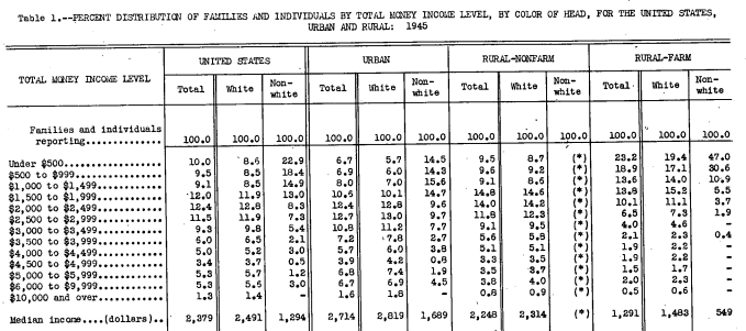
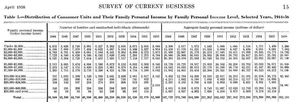
B Proofs of results in Section 3.3

Proof of Proposition 1. By Dinkelbach (1967), an optimizer $\mathbf{y}^{*}_{\max}$ ($\mathbf{y}^{*}_{\min}$) of $G_{n}(\mathbf{y})=(r_{1}(n)^{\top}\mathbf{y})/({r_{2}(n)^{\top}\mathbf{y}})$ also maximizes (minimizes) the linear-form $r_{1}(n)^{\top}\mathbf{y}-G_{n}(\mathbf{y}^{*}_{\max})\,r_{2}(n)^{\top}\mathbf{y}$ (resp. $r_{1}(n)^{\top}\mathbf{y}-G_{n}(\mathbf{y}^{*}_{\min})\,r_{2}(n)^{\top}\mathbf{y}$) under the same constraints. The problem therefore reduces to linear programming with ordering and box constraints, so an optimizer occurs at a vertex of the feasible polyhedron, where necessarily $y_{i}^{*}\in\{\underline{a}_{d(i)},\overline{a}_{d(i)}\}$.

(a) Suppose $\mathbf{y}^{*}_{\min}$ assigns both $\underline{a}_{d}$ and $\overline{a}_{d}$ in group $d$. Then two consecutive entries take these values. Moving them toward each other by $\pm\delta$ with small $\delta>0$ preserves feasibility, ordering, the sum, and yields a vector majorized by $\mathbf{y}^{*}_{\min}$, contradicting optimality under strict Schur-convexity. Hence all entries in each group coincide at the same boundary value.

Next suppose group $d_{0}$ is at $\overline{a}_{d_{0}}$ while some group $d_{1}<d_{0}$ is at $\underline{a}_{d_{1}}$. Increasing the last element of group $d_{1}$ by $\delta>0$ and decreasing the first element of group $d_{0}$ by $\delta$ preserves feasibility, ordering, and the sum, and yields a vector majorized by the original one, strictly lowering the objective. A symmetric argument excludes later groups at the upper boundary when $d_{0}$ is at the lower boundary. Finally, groups $1$ and $D$ must be fixed at $\overline{a}_{1}$ and $\underline{a}_{D}$, respectively; otherwise analogous $\delta$-swaps with neighboring groups reduce the objective.

(b) Suppose some $i_{1}$ satisfies $y^{*}_{i_{1},\max}=\underline{a}_{d(i_{1})}$ while an earlier $i$ has $y^{*}_{i,\max}=\overline{a}_{d(i)}$. Let $i_{1}$ be the largest index in group $d(i_{1})$ at its lower bound and $i$ the smallest index in group $d(i)$ at its upper bound. Replacing $y^{*}_{i_{1},\max}$ by $y^{*}_{i_{1},\max}+\delta$ and $y^{*}_{i,\max}$ by $y^{*}_{i,\max}-\delta$ for small $\delta>0$ preserves feasibility, ordering, and the sum, and produces a vector that majorizes $\mathbf{y}^{*}_{\max}$, contradicting optimality. The symmetric case (a later entry at its lower bound when an earlier one is at its upper bound) yields the same contradiction. Hence at most one group $d_{0}$ may take both boundary values; groups before $d_{0}$ lie at their lower bounds and those after $d_{0}$ at their upper bounds. $\blacksquare$

Proof of Proposition 2. Consider maximization; minimization is identical. By Dinkelbach (1967), any maximizer of $G_{n}$ also maximizes the linear-form $r_{1}(n)^{\top}\mathbf{y}-G_{n}(\mathbf{y}^{*}_{\max})\,r_{2}(n)^{\top}\mathbf{y}$ over the same feasible set, so we may take $\mathbf{y}^{*}_{\max}$ to be a vertex.

(a) Fix group $d$ and hold all other coordinates at their values in $\mathbf{y}^{*}_{\max}$. The resulting linear program in $\mathbf{y}_{d}$ has equality constraints $C^{(1)}_{n,d}\mathbf{y}_{d}=f^{(*1)}_{n,d}$ and $C^{(2)}_{n,d}\mathbf{y}_{d}=f^{(*2)}_{n,d}$, together with within-group ordering and box constraints. At a vertex, $n_{d}$ independent constraints bind. The equalities determine at most $q(d):=\mathrm{rank}([C^{(1)}_{n,d}\;C^{(2)}_{n,d}])\leq q_{1}(d)+q_{2}(d)$ degrees of freedom; the remaining $n_{d}-q(d)$ come from ordering or box constraints. If no ordering constraint binds, these remaining constraints are box constraints, so the group contributes at most $q(d)+2$ distinct values. If $k\geq 1$ ordering constraints bind, they add at most $k$ to rank but introduce no new values, leaving at least $n_{d}-q(d)-k$ box constraints. Hence the same bound $q(d)+2$ still holds.

(b) The same argument applied to the global vertex shows that at most $q\leq q_{1}+q_{2}$ degrees of freedom are pinned down by equality constraints, while the rest are fixed by ordering or box constraints. Box constraints contribute at most the two endpoints in each group, and ordering constraints add no new values. Hence $\mathbf{y}^{*}_{\max}$, and similarly $\mathbf{y}^{*}_{\min}$, has at most $q+2D$ distinct values. $\blacksquare$

Proof of Theorem 1. Let $\mathbf{y}_{d}$ be the subvector of $\mathbf{y}$ for group $d$ with $y_{i}\in[\underline{a}_{d},\overline{a}_{d}]$.

(a) For minimization. Let $\widetilde{\mathbf{y}}$ minimize $G_{n}(\mathbf{y})$ and fix group $d$. Suppose there exist consecutive indices $i,i+1$ with $d(i)=d(i+1)=d$ and $\widetilde{y}_{i}<\widetilde{y}_{i+1}$. Define $\mathbf{y}^{\prime}$ by modifying only these components: $y^{\prime}_{i}=\widetilde{y}_{i}+(\widetilde{y}_{i+1}-\widetilde{y}_{i})/2$ and $y^{\prime}_{i+1}=\widetilde{y}_{i+1}-(\widetilde{y}_{i+1}-\widetilde{y}_{i})/2$. Then $\mathbf{y}^{\prime}$ is majorized by $\widetilde{\mathbf{y}}$, so by Schur-convexity $G_{n}(\mathbf{y}^{\prime})\leq G_{n}(\widetilde{\mathbf{y}})$. If the inequality is strict we contradict optimality; if equality holds we may replace $\widetilde{\mathbf{y}}$ with $\mathbf{y}^{\prime}$. Repeating this averaging step for any unequal consecutive pair in group $d$ yields a minimizer $\mathbf{y}^{*}_{\min}$ in which all components of group $d$ are equal while all constraints remain satisfied.

For maximization. Let $\widetilde{\mathbf{y}}$ maximize $G_{n}(\cdot)$ and fix group $d$. Suppose there exist indices $i<j$ in group $d$ with $\widetilde{y}_{i},\widetilde{y}_{j}\in(\underline{a}_{d},\overline{a}_{d})$. Choose $i$ minimal and $j$ maximal among such indices, so $\widetilde{y}_{i}\leq\widetilde{y}_{j}$. Define $y^{\prime}_{i}=\widetilde{y}_{i}-\delta$ and $y^{\prime}_{j}=\widetilde{y}_{j}+\delta$ with $\delta=\min\{\widetilde{y}_{i}-\underline{a}_{d},\overline{a}_{d}-\widetilde{y}_{j}\}$. Then at least one of $y^{\prime}_{i},y^{\prime}_{j}$ lies on the boundary of $[\underline{a}_{d},\overline{a}_{d}]$. Ordering within group $d$ and the group sum are preserved, so $\mathbf{y}^{\prime}$ majorizes $\widetilde{\mathbf{y}}$, implying $G_{n}(\widetilde{\mathbf{y}})\leq G_{n}(\mathbf{y}^{\prime})$. If the inequality is strict we contradict optimality; otherwise $\mathbf{y}^{\prime}$ is also a maximizer. Repeating this step for the outermost interior pair pushes one element to the boundary without decreasing $G_{n}$ or violating constraints. Continuing until fewer than two interior points remain yields a maximizer with at most one interior coordinate in each group.

(b) For minimization. Let $\widetilde{\mathbf{y}}$ minimize $G_{n}(\mathbf{y})$ and fix group $d$. (i) Consider a block of consecutive elements of group $d$ without constraints in $C_{n}^{(1)}$ or $C_{n}^{(2)}$. If the block contains one element it contributes at most one distinct value. If it contains at least two distinct elements, choose two consecutive ones and apply the transformation in (a), shifting them toward each other while preserving ordering, the group sum, and all constraints. The resulting vector is majorized by $\widetilde{\mathbf{y}}$ and yields a weakly smaller value of $G_{n}$. Repeating this step shows that any such block contributes at most one distinct value; hence all such blocks contribute at most $o_{d}$ distinct values.

(ii) Suppose there are at least $k_{d}+1$ distinct values among the constrained elements of group $d$. By assumption, each block $A^{(d)}_{j}$ has rank 1, so some row of $A^{(d)}_{j}$ contains two consecutive distinct elements. Applying the transformation in (a) makes them coincide while preserving the group sum and all constraints, yielding $\mathbf{y}^{\prime}$. Since $\mathbf{y}^{\prime}$ is majorized by $\widetilde{\mathbf{y}}$, we have $G_{n}(\mathbf{y}^{\prime})\leq G_{n}(\widetilde{\mathbf{y}})$. Repeating this step ensures the elements in $A^{(d)}_{j}$ can be taken equal in an argmin, so the $\widetilde{n}_{d}$ elements of group $d$ contribute at most $k_{d}$ distinct values. $\blacksquare$

For maximization. Let $\widetilde{\mathbf{y}}$ maximize $G_{n}(\mathbf{y})$ and fix group $d$. Let $\mathcal{Y}_{d,\widetilde{n}_{d}}$ denote the set of values taken by the $\widetilde{n}_{d}$ elements for which constraints appear in $\widetilde{\mathcal{C}}_{n,d}$.

(i) Consider a block of consecutive elements in group $d$ with no constraints in $C_{n}^{(1)}$ or $C_{n}^{(2)}$. If the block contains a single element in $(\underline{a}_{d},\overline{a}_{d})$, it contributes at most one distinct value. If it contains at least two distinct elements in $(\underline{a}_{d},\overline{a}_{d})$, select two that are furthest apart and apply the transformation in (a): increase the larger by $\delta>0$ and decrease the smaller by $\delta>0$, preserving the sum and ranking. Increase $\delta$ until one of the elements reaches either a boundary $\underline{a}_{d},\overline{a}_{d}$ or another interior value in $\mathcal{Y}_{d,\widetilde{n}_{d}}$. The resulting vector $\mathbf{y}^{\prime}$ preserves the ranking, the sum, and all constraints in $\widetilde{\mathcal{C}}_{n}$, and majorizes $\widetilde{\mathbf{y}}$, so $G_{n}(\mathbf{y}^{\prime})\geq G_{n}(\widetilde{\mathbf{y}})$. Repeating this step shows that any such block contributes at most one new value beyond $\underline{a}_{d}$, $\overline{a}_{d}$, and the elements of $\mathcal{Y}_{d,\widetilde{n}_{d}}$.

(ii) Suppose there are at least $k_{d}+3$ distinct values among the $\widetilde{n}_{d}$ constrained elements of group $d$. Then some row of $A^{(d)}_{j}$ contains two distinct interior values (different from $\underline{a}_{d},\overline{a}_{d}$). Select two such elements that are furthest apart and apply the same transformation as in (a), pushing them apart by $\delta>0$ while preserving the ranking and the group-$d$ sum. Increase $\delta$ until one element reaches either $\underline{a}_{d}$, $\overline{a}_{d}$, or another interior value in $\mathcal{Y}_{d,\widetilde{n}_{d}}$. The resulting vector $\mathbf{y}^{\prime}$ majorizes $\widetilde{\mathbf{y}}$, so $G_{n}(\mathbf{y}^{\prime})\geq G_{n}(\widetilde{\mathbf{y}})$, and it has one fewer distinct value. Iterating this step ensures that $\mathcal{Y}_{d,\widetilde{n}_{d}}$ contains at most $k_{d}+2$ distinct values, including the two boundaries $\underline{a}_{d}$ and $\overline{a}_{d}$. $\blacksquare$

Proof of Theorem 2. (a) Suppose at least two components indexed by $Q$ lie outside $\mathcal{B}$. Choose one with the largest value and one with the smallest value, say $y^{*}_{i,\max}\geq y^{*}_{j,\max}$, and move them by $\pm\delta$, staying within their intervals, until one reaches $\mathcal{B}$. This preserves feasibility and ranking and yields a vector that majorizes $\mathbf{y}^{*}_{\max}$, so Schur-convexity weakly increases $G_{n}$. Iterating this step produces a maximizer with at most one component outside $\mathcal{B}$.

(b) Suppose there are two distinct values among $\{y^{*}_{i,\min}\}_{i\in Q}$ outside $\mathcal{B}$. Choose two consecutive such values, say $y^{*}_{i,\min}>y^{*}_{j,\min}$, and move them toward each other by $\pm\delta$, staying within their intervals, until they coincide or one reaches $\mathcal{B}$. This preserves feasibility and ranking and yields a vector majorized by $\mathbf{y}^{*}_{\min}$, so Schur-convexity weakly decreases $G_{n}$. Iterating this step produces a minimizer with at most one distinct value outside $\mathcal{B}$. $\blacksquare$

Proof of Theorem 3. Consider maximization; minimization is identical. Fix the ordering induced by a maximizer $\mathbf{y}^{*}_{\max}$, and let $perm(\mathbf{y})$ denote the corresponding permutation. Under this ordering, $G_{n}(\mathbf{y})=\frac{r_{1}(n)^{\top}perm(\mathbf{y})}{r_{2}(n)^{\top}perm(\mathbf{y})}$, and $perm(\mathbf{y}^{*}_{\max})$ maximizes this fraction. By Dinkelbach (1967), it also maximizes $r_{1}(n)^{\top}perm(\mathbf{y})-G_{n}(\mathbf{y}^{*}_{\max})\,r_{2}(n)^{\top}perm(\mathbf{y})$ over the same ordered feasible set. Thus we have a linear program with box constraints $y_{i}\in\mathcal{I}_{i}$ and the imposed ordering, so an optimum is attained at a vertex. Such a vertex can use only values in $\mathcal{U}$: box constraints contribute boundary values, and an active ordering constraint can introduce a new value only by tying an interval observation to a point observation in $P$, in which case the common value is the realized point in $\mathcal{U}$. Combining this with Theorem 2 gives the claim. $\blacksquare$

Proof of Proposition 3. The feasible set is compact and $G_{n}$ is continuous, so minimizers and maximizers exist. We first prove an auxiliary result.

Auxiliary result. Let $a,b,c,d,x^{*}>0$ and define $f(x)=\frac{ax+b}{cx+d}$. For any $\Delta x>0$ with $x^{*}-\Delta x>0$, $f(x^{*}-\Delta x)-f(x^{*})=\frac{\Delta x(bc-ad)}{(c(x^{*}-\Delta x)+d)(cx^{*}+d)}$, which is positive iff $f(x^{*})>a/c$ (equivalently $bc>ad$), and whose absolute value increases with $\Delta x$ until $x^{*}-\Delta x=0$. Similarly, $f(x^{*}+\Delta x)-f(x^{*})=\frac{\Delta x(ad-bc)}{(c(x^{*}+\Delta x)+d)(cx^{*}+d)}$, which is negative iff $f(x^{*})>a/c$ and whose absolute value decreases with $\Delta x$. For any feasible $\mathbf{y}$, let $\mathbf{z}=\mathrm{perm}(\mathbf{y})$ denote its ordered version. Then n2(G_n(z) + n+1n) = (∑_j=1^n j z_j )/∑_j=1^n z_j = ( k z_k + ∑_j ≠k j z_j)/(z_k + ∑_j ≠k z_j), so optimizing $G_{n}$ is equivalent to optimizing $(kz_{k}+\sum_{j\neq k}jz_{j})/(z_{k}+\sum_{j\neq k}z_{j})$.

(a) Let $\mathbf{y}^{*}_{\min}$ be a minimizer satisfying Theorem 3 and let $\mathbf{z}^{*}=\mathrm{perm}(\mathbf{y}^{*}_{\min})$. Define $k^{*}=\left\lceil\frac{n}{2}\bigl(G_{n}(\mathbf{z}^{*})+\frac{n+1}{n}\bigr)\right\rceil$ and $u_{0}=z^{*}_{k^{*}}\in\mathcal{U}$ (ties at $u_{0}$ are immaterial). Consider any $i\in Q$.

If $\overline{a}_{i}<u_{0}$, then $\mathcal{I}_{i}$ lies strictly to the left of $u_{0}$, so $y^{*}_{i,\min}=z^{*}_{j}$ for some $j<k^{*}$. Increasing $z^{*}_{j}$ slightly within $\mathcal{I}_{i}$ (piecewise if ties arise) preserves ordering. Since $j<k^{*}=\lceil\frac{\sum_{\ell=1}^{n}\ell z^{*}_{\ell}}{\sum_{\ell=1}^{n}z^{*}_{\ell}}\rceil$, we have $\frac{\sum_{\ell=1}^{n}\ell z^{*}_{\ell}}{\sum_{\ell=1}^{n}z^{*}_{\ell}}>j$. By the auxiliary result (with $a=j$, $c=1$), increasing $z^{*}_{j}$ strictly decreases the objective and thus $G_{n}$, so optimality requires $y^{*}_{i,\min}=\overline{a}_{i}$. If $\underline{a}_{i}>u_{0}$, then $\mathcal{I}_{i}$ lies strictly to the right of $u_{0}$, so $y^{*}_{i,\min}=z^{*}_{j}$ for some $j>k^{*}$. Decreasing $z^{*}_{j}$ slightly within $\mathcal{I}_{i}$ preserves ordering. Since $j>k^{*}=\lceil\frac{\sum_{\ell=1}^{n}\ell z^{*}_{\ell}}{\sum_{\ell=1}^{n}z^{*}_{\ell}}\rceil$, we have $\frac{\sum_{\ell=1}^{n}\ell z^{*}_{\ell}}{\sum_{\ell=1}^{n}z^{*}_{\ell}}<j$. By the auxiliary result, decreasing $z^{*}_{j}$ strictly decreases the objective and hence $G_{n}$, so optimality requires $y^{*}_{i,\min}=\underline{a}_{i}$. If $u_{0}\in\mathcal{I}_{i}=[\underline{a}_{i},\overline{a}_{i}]$, suppose $y^{*}_{i,\min}<u_{0}$. Then its position in $\mathbf{z}^{*}$ is $j<k^{*}$ and increasing it toward $u_{0}$ strictly decreases $G_{n}(\mathbf{z})$, a contradiction. Similarly, if $y^{*}_{i,\min}>u_{0}$ then $j>k^{*}$ and decreasing it toward $u_{0}$ strictly decreases $G_{n}(\mathbf{z})$. Hence $y^{*}_{i,\min}=u_{0}$.

(b) First show that there exists a maximizer with $y_{i,\max}^{*}\in\mathcal{B}$ for all $i\in Q$. Let $\mathbf{y}_{\max}^{*}$ be a maximizer satisfying Theorem 3. If already $y_{i,\max}^{*}\in\mathcal{B}$ for all $i\in Q$, we are done. Otherwise, by Theorem 3 there is a unique $d\in Q$ with $y_{d,\max}^{*}$ interior to $\mathcal{I}_{d}$. Fix all other components and treat $G_{n}(\mathbf{y})$ as a function of $y_{d}\in\mathcal{I}_{d}$. Let $\mathbf{z}=\mathrm{perm}(\mathbf{y})$ and let $k(d)$ be the position of $y_{d}$ in the ordered vector $\mathbf{z}$. On each region with fixed ordering, $G_{n}(\mathbf{z})$ is continuous and linear-fractional. Its derivative with respect to $z_{k(d)}$ equals $\frac{\partial G_{n}(\mathbf{z})}{\partial z_{k(d)}}=\frac{2}{n}\frac{k(d)q-w}{(q+z_{k(d)})^{2}}$, where $w=\sum_{j\neq k(d)}jz_{j}$ and $q=\sum_{j\neq k(d)}z_{j}$. Hence on each such region the function is either strictly monotone in $z_{k(d)}$ or constant.

When $z_{k(d)}$ increases and crosses a breakpoint where it swaps order with a component of value $v>0$, the index $k(d)$ increases by $1$ and the other component’s index in $w$ decreases by $1$, so $w$ falls by $v$ while $q$ is unchanged. Thus the numerator $k(d)q-w$ increases by $q+v>0$. Consequently the sign of $k(d)q-w$ can change only from negative to positive, never from positive to negative. Therefore, as a function of $y_{d}$ on $\mathcal{I}_{d}$, $G_{n}(\mathbf{z})$ has no interior local maxima: it is either monotone or first decreases and then increases. Hence the maximum over $\mathcal{I}_{d}$ is attained at an endpoint, and by continuity we may replace $y_{d,\max}^{*}$ by either $\underline{a}_{d}$ or $\overline{a}_{d}$ without decreasing $G_{n}$. Thus the maximizer can be taken with $y_{i,\max}^{*}\in\mathcal{B}$ for all $i\in Q$.

Take such a maximizer $\mathbf{y}_{\max}^{*}$ and let $\mathbf{z}^{*}=\mathrm{perm}(\mathbf{y}_{\max}^{*})$. Define $k^{*}=\left\lceil\frac{n}{2}\left(G_{n}(\mathbf{z}^{*})+\frac{n+1}{n}\right)\right\rceil$ and $u_{0}=z_{k^{*}}^{*}\in\mathcal{U}$. If $\overline{a}_{i}<u_{0}$, then $\mathcal{I}_{i}$ lies to the left of $u_{0}$, so $y_{i,\max}^{*}=z_{j}^{*}$ with $j<k^{*}$. By the auxiliary result, decreasing $z_{j}$ increases $G_{n}$, hence optimality requires $y_{i,\max}^{*}=\underline{a}_{i}$. If $\underline{a}_{i}>u_{0}$, then $\mathcal{I}_{i}$ lies to the right of $u_{0}$, so $y_{i,\max}^{*}=z_{j}^{*}$ with $j>k^{*}$. Increasing $z_{j}$ raises $G_{n}$, so optimality requires $y_{i,\max}^{*}=\overline{a}_{i}$. If $u_{0}\in\mathcal{I}_{i}$, then $y_{i,\max}^{*}$ must be one of the endpoints, as already established. $\blacksquare$

C Proofs of results in Section 5

For the proofs in this section, let $h(J),g(J)\subset\mathbb{N}$ index the equality and inequality restrictions included in the $J$-th problem, and write $\mathcal{C}_{J}(c,\theta):=\{\mu\in\mathcal{M}:H(\mu;\theta)_{j}=c_{j}^{1}\ \forall j\in h(J),\ G(\mu;\theta)_{j^{\prime}}\leq c_{j^{\prime}}^{2}\ \forall j^{\prime}\in g(J)\}$. For $a,b\in\mathbb{N}$, let $\Delta^{a-1}:=\{p\in[0,1]^{a}:\sum_{j=1}^{a}p_{j}=1\}$, $b^{-1}\mathbb{Z}_{+}^{a}:=\{p\in\mathbb{R}^{a}:bp\in\mathbb{Z}_{+}^{a}\}$, $\mathcal{C}_{J}^{(a)}(c,\theta):=\mathcal{C}_{J}(c,\theta)\cap\{\sum_{j=1}^{a}p_{j}\delta_{z_{j}}:z\in\mathcal{Y}^{a},\ p\in\Delta^{a-1}\}$, and $\mathcal{C}_{J}^{(a,b)}(c,\theta):=\mathcal{C}_{J}^{(a)}(c,\theta)\cap\{\sum_{j=1}^{a}p_{j}\delta_{z_{j}}:z\in\mathcal{Y}^{a},\ p\in b^{-1}\mathbb{Z}_{+}^{a}\}$. Also write $V_{J}^{a,b,\sup}(\eta):=\sup_{\mu\in\mathcal{C}_{J}^{(a,b)}(c,\theta)}F(\mu;\pi,q)$, $V_{J}^{a,b,\inf}(\eta):=\inf_{\mu\in\mathcal{C}_{J}^{(a,b)}(c,\theta)}F(\mu;\pi,q)$, $V_{J}^{a,\sup}(\eta):=\sup_{\mu\in\mathcal{C}_{J}^{(a)}(c,\theta)}F(\mu;\pi,q)$, $V_{J}^{a,\inf}(\eta):=\inf_{\mu\in\mathcal{C}_{J}^{(a)}(c,\theta)}F(\mu;\pi,q)$, $V_{J}^{\sup}(\eta):=\sup_{\mu\in\mathcal{C}_{J}(c,\theta)}F(\mu;\pi,q)$, and $V_{J}^{\inf}(\eta):=\inf_{\mu\in\mathcal{C}_{J}(c,\theta)}F(\mu;\pi,q)$, with $V_{J}^{a,b}:=(V_{J}^{a,b,\inf},V_{J}^{a,b,\sup})^{\top}$, $V_{J}^{a}:=(V_{J}^{a,\inf},V_{J}^{a,\sup})^{\top}$, and $V_{J}:=(V_{J}^{\inf},V_{J}^{\sup})^{\top}$. Let $\mathcal{L}_{\mathrm{step},n}:=\{u\in\mathcal{L}_{\mathrm{eq},n}\cup\mathcal{L}_{\mathrm{ineq},n}:a_{u,d,n}(\gamma)=0\text{ for all }d\}$, $\mathcal{L}_{\mathrm{aff},n}:=(\mathcal{L}_{\mathrm{eq},n}\cup\mathcal{L}_{\mathrm{ineq},n})\setminus\mathcal{L}_{\mathrm{step},n}$, $\mathcal{L}_{\mathrm{aff,eq},n}:=\mathcal{L}_{\mathrm{eq},n}\setminus\mathcal{L}_{\mathrm{step,eq},n}$, and $m_{\mathrm{aff},n}:=|\mathcal{L}_{\mathrm{aff,eq},n}|$. When $u\in\mathcal{L}_{\mathrm{eq},n}$ we write $c_{u}$ for the corresponding coordinate of $c^{1}$, and when $u\in\mathcal{L}_{\mathrm{ineq},n}$ we write $c_{u}$ for the corresponding coordinate of $c^{2}$; the same convention applies to $\hat{c}_{u}$, $\bar{c}_{u}$, and $c_{m,u}^{*}$. For $x=(p,z)\in\Delta^{k-1}\times\mathcal{Y}^{k}$, let $\mu_{x}:=\sum_{j=1}^{k}p_{j}\delta_{z_{j}}$, $H(x;\theta):=H(\mu_{x};\theta)$, and $G(x;\theta):=G(\mu_{x};\theta)$. For $\circ\in\{\inf,\sup\}$, let $S_{n}^{\circ}(\eta)$ denote the set of optimizers of $V_{J_{n}}^{k_{n},\circ}(\eta)$. If $\mathcal{L}_{\mathrm{aff,eq},n}=\{\ell_{1},\ldots,\ell_{m}\}$ and $j_{1},\ldots,j_{m}$ are selected indices with $p_{j_{t}}>0$, set $S_{\mathrm{aff}}(x,\theta):=(p_{j_{t}}\partial_{y}f_{\ell_{r},n}(z_{j_{t}};\theta))_{t,r}$. If $\mathcal{B}_{\mathrm{step}}=\{\ell_{1},\ldots,\ell_{s}\}\subseteq\mathcal{L}_{\mathrm{step,eq},n}$ and $J_{\mathrm{step}}=\{j_{0},\ldots,j_{s}\}$ are selected indices with $p_{j_{t}}>0$, set $B_{\mathrm{step}}(x,\theta):=((1,f_{\ell_{1},n}(z_{j_{t}};\theta),\ldots,f_{\ell_{s},n}(z_{j_{t}};\theta)))_{t=0}^{s}$; when these sets are chosen relative to a specific optimizer $x^{*}$, write $\mathcal{B}_{\mathrm{step}}(x^{*})$ and $J_{\mathrm{step}}(x^{*})$. For a vector $x$, $(x)_{+}$ denotes the coordinatewise positive part. Fix $0<r_{0}<\tilde{r}_{0}$ so that $\mathcal{N}_{0}:=\{\eta\in\mathbb{H}:\|\eta-\eta_{0}\|_{\infty}\leq r_{0}\}\subset\operatorname{int}(\widetilde{\mathcal{N}}_{0})$, $\widetilde{\mathcal{N}}_{0}:=\{\eta\in\mathbb{H}:\|\eta-\eta_{0}\|_{\infty}\leq\tilde{r}_{0}\}\subset\mathcal{N}_{\eta}$, the $(\pi,q)$-projection of $\widetilde{\mathcal{N}}_{0}$ lies in $\mathcal{N}_{\pi q}$, the $\theta$-projection lies in the neighborhood from Assumption 2, and Assumption 7 holds on $\widetilde{\mathcal{N}}_{0}$. Throughout the local arguments below, the parameter lies in $\mathcal{N}_{0}$. Finally, a restriction is included in the $n$-th problem if it is imposed at $J_{n}$, i.e. if its index lies in $h(J_{n})$ for an equality restriction or in $g(J_{n})$ for an inequality restriction.

Proof of Lemma 1. If $y\in\mathcal{Y}^{N_{2}}$ takes distinct values $z_{1},\ldots,z_{m}$ with multiplicities $r_{1},\ldots,r_{m}$, then $\mu_{y}=\sum_{j=1}^{m}(r_{j}/N_{2})\delta_{z_{j}}$. Padding with repeated support points and zero masses to length $N_{1}$ gives a vector $p\in\Delta^{N_{1}-1}\cap N_{2}^{-1}\mathbb{Z}_{+}^{N_{1}}$, so $\mu_{y}\in\mathcal{C}_{J}^{(N_{1},N_{2})}(c,\theta)$. The converse is immediate from the definition. $\blacksquare$

Lemma 2.

For all integers $N\geq s_{n}+1$ and $J$,

$$\sup_{\begin{subarray}{c}\eta=(c,\theta,\pi,q)\in\mathcal{N}_{0}:\ \mathcal{C}_{J}(c,\theta)\neq\emptyset\end{subarray}}\Big|\sup_{\mu\in\mathcal{C}_{J}(c,\theta)}F(\mu;\pi,q)-\sup_{\mu\in\mathcal{C}_{J}^{(N)}(c,\theta)}F(\mu;\pi,q)\Big|\ \leq\ \bar{C}\cdot\frac{s_{n}}{N},$$

where $\bar{C}:=4L\operatorname{diam}(\mathcal{Y})<\infty$. An analogous bound holds with the outermost $\sup$ replaced by $\inf$.

Proof of Lemma 2. Fix $\eta=(c,\theta,\pi,q)\in\mathcal{N}_{0}$ with $\mathcal{C}_{J}(c,\theta)\neq\varnothing$, and let $N\geq s_{n}+1$. Write the partition as $I_{1,n}(\theta)=[t_{0,n}(\theta),t_{1,n}(\theta)]$ and $I_{d,n}(\theta)=(t_{d-1,n}(\theta),t_{d,n}(\theta)]$ for $d=2,\ldots,s_{n}$. Set $\alpha:=\lfloor(N-1)/s_{n}\rfloor\geq 1$. For each $d$, subdivide $I_{d,n}(\theta)$ into $\alpha$ right-closed subcells $J_{i,d}:=(\xi_{i-1,d},\xi_{i,d}]$, $i=1,\ldots,\alpha$, where $\xi_{0,d}:=t_{d-1,n}(\theta)$, $\xi_{\alpha,d}:=t_{d,n}(\theta)$, and the lengths $\xi_{i,d}-\xi_{i-1,d}$ are all equal. Let $\Delta_{N}:=\max_{d,i}(\xi_{i,d}-\xi_{i-1,d})$. Take any $\mu\in\mathcal{C}_{J}(c,\theta)$. For each $(i,d)$ let $w_{i,d}:=\mu(J_{i,d})$. If $w_{i,d}>0$, let $\mu_{i,d}:=\mu(\cdot\cap J_{i,d})/w_{i,d}$ and $\bar{x}_{i,d}:=\int x\,d\mu_{i,d}(x)\in J_{i,d}$; if $w_{i,d}=0$, pick any $\bar{x}_{i,d}\in J_{i,d}$. Define $\mu_{N}:=\mu(\{t_{0,n}(\theta)\})\delta_{t_{0,n}(\theta)}+\sum_{d=1}^{s_{n}}\sum_{i=1}^{\alpha}w_{i,d}\delta_{\bar{x}_{i,d}}$. Then $\mu_{N}$ is a probability measure and $\#\operatorname{supp}(\mu_{N})\leq 1+\alpha s_{n}\leq N$.

We claim $\mu_{N}\in\mathcal{C}_{J}(c,\theta)$. Fix any row $\ell\in\mathcal{L}_{\mathrm{eq},n}\cup\mathcal{L}_{\mathrm{ineq},n}$. If $\ell\in\mathcal{L}_{\mathrm{step},n}$, then $f_{\ell,n}(\cdot;\theta)$ is constant on each cell $I_{d,n}(\theta)$, hence on each subcell $J_{i,d}$, so $\int_{J_{i,d}}f_{\ell,n}(y;\theta)\,d\mu_{N}(y)=f_{\ell,n}(\bar{x}_{i,d};\theta)\,w_{i,d}=\int_{J_{i,d}}f_{\ell,n}(y;\theta)\,d\mu(y)$. If instead $\ell\in\mathcal{L}_{\mathrm{aff},n}$, then by Assumption 2 there exist coefficients $a_{\ell,d,n}(\theta)$ and $b_{\ell,d,n}(\theta)$ such that $f_{\ell,n}(y;\theta)=a_{\ell,d,n}(\theta)\,y+b_{\ell,d,n}(\theta)$ for $y\in I_{d,n}(\theta)$, and therefore on each $J_{i,d}\subseteq I_{d,n}(\theta)$, $\int_{J_{i,d}}f_{\ell,n}(y;\theta)\,d\mu_{N}(y)=w_{i,d}\{a_{\ell,d,n}(\theta)\bar{x}_{i,d}+b_{\ell,d,n}(\theta)\}=\int_{J_{i,d}}f_{\ell,n}(y;\theta)\,d\mu(y)$. The atom at $t_{0,n}(\theta)$ is left unchanged, so summing over $(i,d)$ gives $\int f_{\ell,n}(y;\theta)\,d\mu_{N}(y)=\int f_{\ell,n}(y;\theta)\,d\mu(y)$ for every included row $\ell$. Hence $\mu_{N}\in\mathcal{C}_{J}(c,\theta)$, and because $\#\operatorname{supp}(\mu_{N})\leq N$, also $\mu_{N}\in\mathcal{C}_{J}^{(N)}(c,\theta)$. Next define a coupling by $\gamma:=\mu(\{t_{0,n}(\theta)\})\delta_{(t_{0,n}(\theta),t_{0,n}(\theta))}+\sum_{d=1}^{s_{n}}\sum_{i=1}^{\alpha}w_{i,d}\,\mu_{i,d}\otimes\delta_{\bar{x}_{i,d}}$. Then $\gamma$ is a coupling of $(\mu,\mu_{N})$, and because $|x-x^{\prime}|\leq\Delta_{N}$ on each $J_{i,d}\times J_{i,d}$, $W_{1}(\mu,\mu_{N})\leq\int|x-x^{\prime}|\,d\gamma(x,x^{\prime})\leq\Delta_{N}$. Assumption 3(i) therefore gives $|F(\mu;\pi,q)-F(\mu_{N};\pi,q)|\leq L\,\Delta_{N}$.

Let $V(\pi,q):=\sup_{\tilde{\mu}\in\mathcal{C}_{J}(c,\theta)}F(\tilde{\mu};\pi,q)$ and $V_{N}(\pi,q):=\sup_{\tilde{\mu}\in\mathcal{C}_{J}^{(N)}(c,\theta)}F(\tilde{\mu};\pi,q)$. Since $\mathcal{C}_{J}^{(N)}(c,\theta)\subseteq\mathcal{C}_{J}(c,\theta)$, we have $V_{N}(\pi,q)\leq V(\pi,q)$. Conversely, for any $\varepsilon>0$, choose $\mu^{\varepsilon}\in\mathcal{C}_{J}(c,\theta)$ with $F(\mu^{\varepsilon};\pi,q)\geq V(\pi,q)-\varepsilon$ and apply the construction above to obtain $\mu_{N}^{\varepsilon}\in\mathcal{C}_{J}^{(N)}(c,\theta)$ with $F(\mu_{N}^{\varepsilon};\pi,q)\geq F(\mu^{\varepsilon};\pi,q)-L\Delta_{N}$. Hence $V_{N}(\pi,q)\geq V(\pi,q)-\varepsilon-L\Delta_{N}$, and letting $\varepsilon\downarrow 0$ yields $|V(\pi,q)-V_{N}(\pi,q)|\leq L\Delta_{N}$. Finally, $\Delta_{N}\leq\operatorname{diam}(\mathcal{Y})/\alpha$ and $\alpha=\lfloor(N-1)/s_{n}\rfloor\geq(N-1)/(2s_{n})$ for $N\geq s_{n}+1$, so $\Delta_{N}\leq\frac{2s_{n}\operatorname{diam}(\mathcal{Y})}{N-1}\leq\frac{4s_{n}\operatorname{diam}(\mathcal{Y})}{N}$. Therefore $|V(\pi,q)-V_{N}(\pi,q)|\leq 4L\operatorname{diam}(\mathcal{Y})\,\frac{s_{n}}{N}$. Taking suprema over admissible $(c,\theta)$ and $(\pi,q)$ yields the claimed bound. The infimum case follows by applying the same argument to $-F$, which is also $L$-Lipschitz in $W_{1}$. $\blacksquare$

Lemma 3.

For all large $n$, there exist $N_{2,0},K<\infty$ such that the following holds uniformly over $N_{1}\geq k_{n}$ and $\eta=(c,\theta,\pi,q)\in\widetilde{\mathcal{N}}_{0}$: if $N_{2}\geq N_{2,0}$, $c_{u}\in N_{2}^{-1}\mathbb{Z}$ for every $u\in\mathcal{L}_{\mathrm{step,eq},n}$, and $\mu\in\mathcal{C}_{J_{n}}^{(N_{1})}(c,\theta)$, then there exists $\tilde{\mu}\in\mathcal{C}_{J_{n}}^{(N_{1},N_{2})}(c,\theta)$ with $W_{1}(\mu,\tilde{\mu})\leq K/N_{2}$.

Proof of Lemma 3. Let $m_{0}:=m_{\mathrm{aff},n}$. Choose an $N_{1}$-point representation $\mu=\sum_{j=1}^{N_{1}}p_{j}\delta_{z_{j}}$. If $m_{0}>0$, choose this representation and distinct indices $j_{1},\dots,j_{m_{0}}$ as in Assumption 7(b); if $m_{0}=0$, interpret $\{j_{1},\dots,j_{m_{0}}\}$ as the empty set. Write $x:=(p,z)$ and $M:=\bar{f}^{\prime}$. Let $\mu^{\mathrm{sl}}=\sum_{j=1}^{N_{1}}p_{j}^{\mathrm{sl}}\delta_{z_{j}}\in\mathcal{C}_{J_{n}}^{(N_{1})}(c,\theta)$ be a comparison measure with the same support points such that $c_{\ell}-\int f_{\ell,n}(y;\theta)\,d\mu^{\mathrm{sl}}(y)\geq\underline{s}$ for all $\ell\in\mathcal{L}_{\mathrm{ineq},n}$; this exists by Assumption 7(a). Choose $a>0$ so large that $a\underline{s}\geq 2(m_{0}+1)+\{M+2m_{0}M^{2}\bar{C}_{\mathrm{slope}}/\underline{p}\}(m_{0}+1)\operatorname{diam}(\mathcal{Y})$. Next choose $N_{2,0}<\infty$ so large that, for every $N_{2}\geq N_{2,0}$, $a/N_{2}<1$, $(m_{0}+1+a)/N_{2}\leq\underline{p}/2$, and $2m_{0}M(m_{0}+1)\bar{C}_{\mathrm{slope}}\operatorname{diam}(\mathcal{Y})/N_{2}<\underline{\delta}$. Fix such an $N_{2}$, set $\alpha:=a/N_{2}$, and define $\mu_{1}:=(1-\alpha)\mu+\alpha\mu^{\mathrm{sl}}=\sum_{j=1}^{N_{1}}p_{j}^{(1)}\delta_{z_{j}}$. Then $\mu_{1}$ satisfies all equalities, every included inequality has slack at least $\alpha\underline{s}$, and $W_{1}(\mu,\mu_{1})\leq\alpha\operatorname{diam}(\mathcal{Y})$.

Let $\tau_{0}<\cdots<\tau_{B}$ be the ordered distinct collection of $\underline{y}$, $\overline{y}$, all endpoints of included step-function equality restrictions, and all partition boundaries at which some row in $\mathcal{L}_{\mathrm{aff},n}$ changes affine formula. Write $K_{1}:=[\tau_{0},\tau_{1}]$ and $K_{b}:=(\tau_{b-1},\tau_{b}]$ for $b=2,\dots,B$. For each $b=1,\dots,B-1$, Assumption 2(iii) implies that the cumulative row $u_{b}:y\mapsto\mathbf{1}\{y\leq\tau_{b}\}$ belongs to $\mathcal{L}_{\mathrm{step,eq},n}$. Because $\mu_{1}$ satisfies all equalities and the lemma hypothesis gives $c_{u_{b}}\in N_{2}^{-1}\mathbb{Z}$, we have $\mu_{1}((-\infty,\tau_{b}])=c_{u_{b}}\in N_{2}^{-1}\mathbb{Z}$. Hence $\mu_{1}(K_{1})=\mu_{1}((-\infty,\tau_{1}])\in N_{2}^{-1}\mathbb{Z}$, $\mu_{1}(K_{b})=\mu_{1}((-\infty,\tau_{b}])-\mu_{1}((-\infty,\tau_{b-1}])\in N_{2}^{-1}\mathbb{Z}$ for $b=2,\dots,B-1$, and $\mu_{1}(K_{B})=1-\mu_{1}((-\infty,\tau_{B-1}])\in N_{2}^{-1}\mathbb{Z}$.

For each block $K_{b}$, let $q_{b}$ be the number of support points of $\mu_{1}$ in $K_{b}$. If $q_{b}=0$, then $\mu_{1}(K_{b})=0$ and we leave that block unchanged. If $q_{b}>0$, list its atoms as $(z_{b,r},p_{b,r}^{(1)},i_{b,r})_{r=1}^{q_{b}}$ in increasing order of $z_{b,r}$, and write $P_{b,r}^{(1)}:=\sum_{u=1}^{r}p_{b,u}^{(1)}$. Set $S_{b,0}:=0$. For $r=1,\dots,q_{b}-1$, let $S_{b,r}:=S_{b,r-1}+\lfloor N_{2}p_{b,r}^{(1)}\rfloor/N_{2}$ if $i_{b,r}\in\{j_{1},\dots,j_{m_{0}}\}$, and let $S_{b,r}:=\lfloor N_{2}P_{b,r}^{(1)}\rfloor/N_{2}$ otherwise. Then $S_{b,r-1}\leq S_{b,r}\leq\mu_{1}(K_{b})$ and $S_{b,r}\in N_{2}^{-1}\mathbb{Z}$. Set $p_{b,r}^{(2)}:=S_{b,r}-S_{b,r-1}$ for $r<q_{b}$ and $p_{b,q_{b}}^{(2)}:=\mu_{1}(K_{b})-S_{b,q_{b}-1}$. If $e_{b,r}:=P_{b,r}^{(1)}-S_{b,r}$, then $0\leq e_{b,r}<1/N_{2}$ whenever $i_{b,r}\notin\{j_{1},\dots,j_{m_{0}}\}$, while $e_{b,r}=e_{b,r-1}+p_{b,r}^{(1)}-\lfloor N_{2}p_{b,r}^{(1)}\rfloor/N_{2}$ whenever $i_{b,r}\in\{j_{1},\dots,j_{m_{0}}\}$. Since there are at most $m_{0}$ selected indices in total, it follows by induction that $0\leq e_{b,r}\leq(m_{0}+1)/N_{2}$ for all $r<q_{b}$, and $e_{b,q_{b}}=0$.

Doing this block by block defines $\mu_{2}:=\sum_{j=1}^{N_{1}}p_{j}^{(2)}\delta_{z_{j}}$. All weights are nonnegative, belong to $N_{2}^{-1}\mathbb{Z}_{+}$, and preserve each block mass exactly. Hence $\sup_{y}|\mu_{2}((-\infty,y])-\mu_{1}((-\infty,y])|\leq(m_{0}+1)/N_{2}$, so $W_{1}(\mu_{2},\mu_{1})\leq(m_{0}+1)\operatorname{diam}(\mathcal{Y})/N_{2}$. Every included step equality is preserved exactly, because each included step-function equality restriction is an interval indicator with endpoints in $\{\tau_{0},\dots,\tau_{B}\}$. Let $\lambda:=\mu_{2}-\mu_{1}$. Then $\lambda(K_{b})=0$ for every $b$. For $\ell\in\mathcal{L}_{\mathrm{aff,eq},n}$, writing $f_{\ell,n}(y;\theta)=a_{\ell,b}y+b_{\ell,b}$ on $K_{b}$ with $|a_{\ell,b}|\leq M$, blockwise integration by parts gives

$$|\int f_{\ell,n}(y;\theta)\,d\lambda(y)|\leq M\sum_{b=1}^{B}\int_{K_{b}}|\lambda((-\infty,y])|\,dy\leq M(m_{0}+1)\operatorname{diam}(\mathcal{Y})/N_{2}.$$

Therefore, if $r_{\ell}:=\int f_{\ell,n}(y;\theta)\,d\mu_{2}(y)-c_{\ell}$, then $\|r\|_{\infty}\leq M(m_{0}+1)\operatorname{diam}(\mathcal{Y})/N_{2}$.

If $m_{0}=0$, set $\tilde{\mu}:=\mu_{2}$ and $\beta:=0$. If $m_{0}>0$, then $|p_{j_{t}}^{(2)}-p_{j_{t}}|\leq|p_{j_{t}}^{(2)}-p_{j_{t}}^{(1)}|+|p_{j_{t}}^{(1)}-p_{j_{t}}|\leq(m_{0}+1+a)/N_{2}\leq\underline{p}/2\leq p_{j_{t}}/2$, so $p_{j_{t}}^{(2)}\geq p_{j_{t}}/2$. Let $D:=\operatorname{diag}(p_{j_{1}},\dots,p_{j_{m_{0}}})$, $D_{2}:=\operatorname{diag}(p_{j_{1}}^{(2)},\dots,p_{j_{m_{0}}}^{(2)})$, and $x_{2}:=(p^{(2)},z)$. Then $S_{\mathrm{aff}}(x_{2},\theta)^{-1}=S_{\mathrm{aff}}(x,\theta)^{-1}DD_{2}^{-1}$ and $\|DD_{2}^{-1}\|_{\infty}\leq 2$, so $\|S_{\mathrm{aff}}(x_{2},\theta)^{-1}\|_{\infty}\leq 2\bar{C}_{\mathrm{slope}}$. Define $\Delta:=-(S_{\mathrm{aff}}(x_{2},\theta)^{\top})^{-1}r$. Since $\|(S_{\mathrm{aff}}(x_{2},\theta)^{\top})^{-1}\|_{\infty}=\|S_{\mathrm{aff}}(x_{2},\theta)^{-1}\|_{1}\leq m_{0}\|S_{\mathrm{aff}}(x_{2},\theta)^{-1}\|_{\infty}$, we have $\beta:=\|\Delta\|_{\infty}\leq 2m_{0}M(m_{0}+1)\bar{C}_{\mathrm{slope}}\operatorname{diam}(\mathcal{Y})/N_{2}<\underline{\delta}$. Let $\tilde{\mu}$ be obtained from $\mu_{2}$ by replacing each $z_{j_{t}}$ with $z_{j_{t}}+\Delta_{t}$. Then every selected support point stays in the same partition cell, every moment equality is repaired exactly because affine restrictions are affine on that cell, and every step equality remains unchanged because step-function restrictions are constant on partition cells.

It remains to check the inequalities. If $\ell\in\mathcal{L}_{\mathrm{step},n}$, then moving atoms from $\mu_{2}$ to $\tilde{\mu}$ does not change the row. Since every included step-function restriction is an interval indicator and $\sup_{y}|\mu_{2}((-\infty,y])-\mu_{1}((-\infty,y])|\leq(m_{0}+1)/N_{2}$, we have $\left|\int f_{\ell,n}(y;\theta)\,d\tilde{\mu}(y)-\int f_{\ell,n}(y;\theta)\,d\mu_{1}(y)\right|=\left|\mu_{2}(I)-\mu_{1}(I)\right|\leq 2(m_{0}+1)/N_{2}$. If $\ell\in\mathcal{L}_{\mathrm{aff},n}$, the same integration-by-parts argument applied to $\tilde{\mu}-\mu_{1}$ gives $\left|\int f_{\ell,n}(y;\theta)\,d\tilde{\mu}(y)-\int f_{\ell,n}(y;\theta)\,d\mu_{1}(y)\right|\leq M\,W_{1}(\tilde{\mu},\mu_{1})\leq M\{(m_{0}+1)\operatorname{diam}(\mathcal{Y})/N_{2}+\beta\}$, because $W_{1}(\tilde{\mu},\mu_{2})\leq\sum_{t=1}^{m_{0}}p_{j_{t}}^{(2)}|\Delta_{t}|\leq\beta$. By the choice of $a$, both bounds are at most $\alpha\underline{s}$. Since $\mu_{1}$ has slack $\alpha\underline{s}$ on every inequality restriction, all included inequalities remain feasible. Therefore $\tilde{\mu}\in\mathcal{C}_{J_{n}}^{(N_{1},N_{2})}(c,\theta)$. Finally, $W_{1}(\mu,\tilde{\mu})\leq W_{1}(\mu,\mu_{1})+W_{1}(\mu_{1},\mu_{2})+W_{1}(\mu_{2},\tilde{\mu})\leq a\operatorname{diam}(\mathcal{Y})/N_{2}+(m_{0}+1)\operatorname{diam}(\mathcal{Y})/N_{2}+\beta$, which is at most $K/N_{2}$ for some finite constant $K$. $\blacksquare$

Lemma 4.

Let $N_{1}\geq k_{n}$, let $N_{2}$ be large enough that Lemma 3 applies, and let $\eta=(c,\theta,\pi,q)\in\widetilde{\mathcal{N}}_{0}$ satisfy $\mathcal{C}_{J_{n}}^{(N_{1})}(c,\theta)\neq\varnothing$. Suppose $c_{u}\in N_{2}^{-1}\mathbb{Z}$ for every $u\in\mathcal{L}_{\mathrm{step,eq},n}$. Then $\mathcal{C}_{J_{n}}^{(N_{1},N_{2})}(c,\theta)\neq\varnothing$ and $\|V_{J_{n}}^{N_{1}}(\eta)-V_{J_{n}}^{N_{1},N_{2}}(\eta)\|_{2}\leq\sqrt{2}\,LK/N_{2}$.

Proof of Lemma 4. Lemma 3 yields $\mathcal{C}_{J_{n}}^{(N_{1},N_{2})}(c,\theta)\neq\varnothing\subseteq\mathcal{C}_{J_{n}}^{(N_{1})}(c,\theta)$, so the supremum difference is nonnegative. Let $\varepsilon>0$ and choose $\mu\in\mathcal{C}_{J_{n}}^{(N_{1})}(c,\theta)$ such that $F(\mu;\pi,q)\geq\sup_{\nu\in\mathcal{C}_{J_{n}}^{(N_{1})}(c,\theta)}F(\nu;\pi,q)-\varepsilon$. By Lemma 3, there exists $\tilde{\mu}\in\mathcal{C}_{J_{n}}^{(N_{1},N_{2})}(c,\theta)$ with $W_{1}(\mu,\tilde{\mu})\leq K/N_{2}$. Assumption 3(i) therefore gives

$$F(\mu;\pi,q)\leq F(\tilde{\mu};\pi,q)+LK/N_{2}\leq\sup_{\nu\in\mathcal{C}_{J_{n}}^{(N_{1},N_{2})}(c,\theta)}F(\nu;\pi,q)+LK/N_{2}.$$

Letting $\varepsilon\downarrow 0$ proves the supremum bound. The infimum coordinate follows by applying the same argument to $-F$, and the vector bound is immediate. $\blacksquare$

Lemma 5.

There exist constants $\Delta_{0}>0$ and $C<\infty$ such that the following holds for all sufficiently large $n$. Let $N\geq k_{n}$, let $\eta=(c,\theta,\pi,q)$ and $\bar{\eta}=(\bar{c},\theta,\pi,q)$ lie in $\widetilde{\mathcal{N}}_{0}$, let $\tau_{0}<\cdots<\tau_{B}$ be the ordered distinct collection of $\underline{y}$, $\overline{y}$, all endpoints of included step-function equality restrictions, and all partition boundaries at which some row in $\mathcal{L}_{\mathrm{aff},n}$ changes affine formula, and write $K_{1}:=[\tau_{0},\tau_{1}]$ and $K_{b}:=(\tau_{b-1},\tau_{b}]$ for $b=2,\dots,B$. Suppose $\bar{c}$ agrees with $c$ on $\mathcal{L}_{\mathrm{aff,eq},n}$ and on the inequality coordinates, let $u_{b}\in\mathcal{L}_{\mathrm{step,eq},n}$ denote the cumulative row $y\mapsto\mathbf{1}\{y\leq\tau_{b}\}$ for $b=1,\dots,B-1$, define $m_{1}:=c_{u_{1}}$, $m_{b}:=c_{u_{b}}-c_{u_{b-1}}$ for $b=2,\dots,B-1$, and $m_{B}:=1-c_{u_{B-1}}$, and define $\bar{m}_{b}$ from $\bar{c}$ in the same way. If $m_{b}=0$ if and only if $\bar{m}_{b}=0$ for every $b$, $\Delta:=\sum_{b=1}^{B}|\bar{m}_{b}-m_{b}|\leq\Delta_{0}$, and at least one of $\mathcal{C}_{J_{n}}^{(N)}(c,\theta)$ and $\mathcal{C}_{J_{n}}^{(N)}(\bar{c},\theta)$ is nonempty, then both are nonempty and $\|V_{J_{n}}^{N}(\eta)-V_{J_{n}}^{N}(\bar{\eta})\|_{2}\leq\sqrt{2}\,LC\,\Delta$.

Proof of Lemma 5. By symmetry it suffices to assume $\mathcal{C}_{J_{n}}^{(N)}(c,\theta)\neq\emptyset$. We first prove the bound for the supremum coordinate. Fix $\varepsilon>0$. Choose an $N$-point representation $\mu=\sum_{j=1}^{N}p_{j}\delta_{z_{j}}\in\mathcal{C}_{J_{n}}^{(N)}(c,\theta)$ together with selected indices $j_{1},\dots,j_{m_{\mathrm{aff},n}}$ as in Assumption 7(b) and such that $F(\mu;\pi,q)\geq V_{J_{n}}^{N,\sup}(\eta)-\varepsilon$. Let $\mu^{\mathrm{sl}}=\sum_{j=1}^{N}p_{j}^{\mathrm{sl}}\delta_{z_{j}}$ be the comparison measure with the same support points from Assumption 7(a). Set $C_{\mathrm{rep}}:=2m_{\mathrm{aff}}\bar{C}_{\mathrm{slope}}$ and $C_{\mathrm{feas}}:=1+\bar{f}^{\prime}C_{\mathrm{rep}}$. Choose $a>0$ so large that $a\underline{s}\geq C_{\mathrm{feas}}\bar{f}$, set $\alpha:=a\Delta$, and define $\mu_{1}:=(1-\alpha)\mu+\alpha\mu^{\mathrm{sl}}$. For $\Delta_{0}$ small enough, $\alpha<1$, $(1-\alpha)\underline{p}-\Delta\geq\underline{p}/2$, and $C_{\mathrm{rep}}\bar{f}\Delta<\underline{\delta}$ whenever $\Delta\leq\Delta_{0}$. By Assumption 7(a), $\mu_{1}\in\mathcal{C}_{J_{n}}^{(N)}(c,\theta)$ and $c_{\ell}-\int f_{\ell,n}(y;\theta)\,d\mu_{1}(y)\geq\alpha\underline{s}$ for every $\ell\in\mathcal{L}_{\mathrm{ineq},n}$.

For each block $K_{b}$ with $m_{b}>0$, let $\nu_{b}:=\mu_{1}(\cdot\cap K_{b})/m_{b}$. If $m_{b}=0$, choose any probability measure $\nu_{b}$ supported on $K_{b}$; this is harmless as then $\bar{m}_{b}=0$ as well. Define $\mu_{2}:=\sum_{b=1}^{B}\bar{m}_{b}\nu_{b}$. It is supported on the same atoms as $\mu_{1}$, satisfies $\mu_{2}(K_{b})=\bar{m}_{b}$ for every $b$, and hence satisfies all included step equalities under $\bar{c}$. Let $\delta_{b}:=\bar{m}_{b}-m_{b}$, so $\sum_{b=1}^{B}\delta_{b}=0$ and $\sum_{b=1}^{B}|\delta_{b}|\leq\Delta$. For any $1$-Lipschitz $g$ on $\mathcal{Y}$, subtracting the constant $g(\underline{y})$ gives $\|g-g(\underline{y})\|_{\infty}\leq\operatorname{diam}(\mathcal{Y})$, hence $|\int g\,d\mu_{2}-\int g\,d\mu_{1}|=|\sum_{b=1}^{B}\delta_{b}\int g\,d\nu_{b}|\leq\operatorname{diam}(\mathcal{Y})\Delta$. Therefore $W_{1}(\mu_{1},\mu_{2})\leq\operatorname{diam}(\mathcal{Y})\Delta$. Likewise, since $|f_{\ell,n}(y;\theta)|\leq\bar{f}$, $|\int f_{\ell,n}(y;\theta)\,d\mu_{2}(y)-\int f_{\ell,n}(y;\theta)\,d\mu_{1}(y)|=|\sum_{b=1}^{B}\delta_{b}\int f_{\ell,n}(y;\theta)\,d\nu_{b}(y)|\leq\bar{f}\Delta$ for each included row $\ell$. In particular, if $r_{\ell}:=\int f_{\ell,n}(y;\theta)\,d\mu_{2}(y)-c_{\ell}$ for $\ell\in\mathcal{L}_{\mathrm{aff,eq},n}$, then $\|r\|_{\infty}\leq\bar{f}\Delta$. Moreover, if $z_{j_{t}}\in K_{b(t)}$, then $p_{j_{t}}^{(2)}=p_{j_{t}}^{(1)}\bar{m}_{b(t)}/m_{b(t)}$ whenever $m_{b(t)}>0$, so $|p_{j_{t}}^{(2)}-p_{j_{t}}^{(1)}|\leq|\bar{m}_{b(t)}-m_{b(t)}|\leq\Delta$. Hence $p_{j_{t}}^{(2)}\geq p_{j_{t}}^{(1)}-\Delta\geq(1-\alpha)p_{j_{t}}-\Delta\geq p_{j_{t}}/2\geq\underline{p}/2$.

If $m_{\mathrm{aff},n}=0$, set $\tilde{\mu}:=\mu_{2}$. If $m_{\mathrm{aff},n}>0$, let $D:=\operatorname{diag}(p_{j_{1}},\dots,p_{j_{m_{\mathrm{aff},n}}})$, let $D_{2}:=\operatorname{diag}(p_{j_{1}}^{(2)},\dots,p_{j_{m_{\mathrm{aff},n}}}^{(2)})$, and let $x_{2}:=(p^{(2)},z)$. Then $S_{\mathrm{aff}}(x_{2},\theta)=D_{2}D^{-1}S_{\mathrm{aff}}(x,\theta)$, so $S_{\mathrm{aff}}(x_{2},\theta)^{-1}=S_{\mathrm{aff}}(x,\theta)^{-1}DD_{2}^{-1}$ and $\|DD_{2}^{-1}\|_{\infty}\leq 2$. Hence $\|S_{\mathrm{aff}}(x_{2},\theta)^{-1}\|_{\infty}\leq 2\bar{C}_{\mathrm{slope}}$. Define $\Delta^{\mathrm{aff}}:=-(S_{\mathrm{aff}}(x_{2},\theta)^{\top})^{-1}r$. Since $\|(S_{\mathrm{aff}}(x_{2},\theta)^{\top})^{-1}\|_{\infty}=\|S_{\mathrm{aff}}(x_{2},\theta)^{-1}\|_{1}\leq 2m_{\mathrm{aff}}\bar{C}_{\mathrm{slope}}=C_{\mathrm{rep}}$, we have $\|\Delta^{\mathrm{aff}}\|_{\infty}\leq C_{\mathrm{rep}}\bar{f}\Delta<\underline{\delta}$. Let $\tilde{\mu}$ be obtained from $\mu_{2}$ by replacing each selected support point $z_{j_{t}}$ with $z_{j_{t}}+\Delta_{t}^{\mathrm{aff}}$. Then the selected support points stay in their original partition cells, every moment equality is repaired exactly since affine restrictions are affine on those cells, and every step equality remains unchanged because step-function restrictions are constant on partition cells.

Moving from $\mu_{1}$ to $\mu_{2}$ changes any included inequality restriction by at most $\bar{f}\Delta$. Moving from $\mu_{2}$ to $\tilde{\mu}$ does not affect step-function restrictions and changes any affine restriction by at most $\bar{f}^{\prime}\|\Delta^{\mathrm{aff}}\|_{\infty}\leq\bar{f}^{\prime}C_{\mathrm{rep}}\bar{f}\Delta$. Hence the total inequality change is at most $C_{\mathrm{feas}}\bar{f}\Delta\leq\alpha\underline{s}$, so the slack created in $\mu_{1}$ is preserved and $\tilde{\mu}\in\mathcal{C}_{J_{n}}^{(N)}(\bar{c},\theta)$. Therefore $\mathcal{C}_{J_{n}}^{(N)}(\bar{c},\theta)\neq\emptyset$. Also, $W_{1}(\mu,\tilde{\mu})\leq W_{1}(\mu,\mu_{1})+W_{1}(\mu_{1},\mu_{2})+W_{1}(\mu_{2},\tilde{\mu})\leq a\operatorname{diam}(\mathcal{Y})\Delta+\operatorname{diam}(\mathcal{Y})\Delta+C_{\mathrm{rep}}\bar{f}\Delta=:C\Delta$. Assumption 3(i) therefore gives $V_{J_{n}}^{N,\sup}(\eta)-\varepsilon\leq F(\mu;\pi,q)\leq F(\tilde{\mu};\pi,q)+LC\Delta\leq V_{J_{n}}^{N,\sup}(\bar{\eta})+LC\Delta$. Letting $\varepsilon\downarrow 0$ yields $V_{J_{n}}^{N,\sup}(\eta)-V_{J_{n}}^{N,\sup}(\bar{\eta})\leq LC\Delta$. Reversing the roles of $\eta$ and $\bar{\eta}$ gives the reverse inequality. The infimum coordinate follows by applying the same argument to $-F$, and the vector bound is immediate. $\blacksquare$

Lemma 6.

$\sup_{\eta\in\mathcal{N}_{0}}\|V_{J_{n}}(\eta)-V_{J_{n}}^{k_{n}}(\eta)\|_{2}=o(n^{-1/2})$.

Proof of Lemma 6. We first prove the claim for the supremum coordinate; the infimum coordinate then follows by applying the same argument to $-F$. Set $N_{1}:=\lceil 2n(s_{n}+1)^{2}\rceil$ and $N_{2}:=nN_{1}$. Then $N_{1}\geq n\geq k_{n}$, $s_{n}/N_{1}\leq\{2n(s_{n}+1)\}^{-1}$, and $1/N_{2}=O(n^{-2})$. Fix $\eta=(c,\theta,\pi,q)\in\mathcal{N}_{0}$. Let $\tau_{0}<\cdots<\tau_{B}$ be the ordered distinct collection of $\underline{y}$, $\overline{y}$, all endpoints of included step-function equality restrictions, and all partition boundaries at which some row in $\mathcal{L}_{\mathrm{aff},n}$ changes affine formula, and write $K_{1}:=[\tau_{0},\tau_{1}]$ and $K_{b}:=(\tau_{b-1},\tau_{b}]$ for $b=2,\dots,B$. For $b=1,\dots,B-1$, let $u_{b}\in\mathcal{L}_{\mathrm{step,eq},n}$ denote the cumulative row $y\mapsto\mathbf{1}\{y\leq\tau_{b}\}$ guaranteed by Assumption 2(iii). Define $m_{1}:=c_{u_{1}}$, $m_{b}:=c_{u_{b}}-c_{u_{b-1}}$ for $b=2,\dots,B-1$, and $m_{B}:=1-c_{u_{B-1}}$. Since $\mathcal{C}_{\infty}(c,\theta)\neq\emptyset$ by Assumption  7(a), these block masses are nonnegative and sum to one.

Choose $b_{*}$ among the positive blocks so that $m_{b_{*}}=\max\{m_{b}:m_{b}>0\}$. Define $\bar{m}_{b}:=0$ if $m_{b}=0$, $\bar{m}_{b}:=N_{2}^{-1}\max\{1,\lfloor N_{2}m_{b}\rfloor\}$ if $m_{b}>0$ and $b\neq b_{*}$, and $\bar{m}_{b_{*}}:=1-\sum_{r\neq b_{*}}\bar{m}_{r}$. Then $\bar{m}_{b}\in N_{2}^{-1}\mathbb{Z}_{+}$ for every $b$, $\sum_{b=1}^{B}\bar{m}_{b}=1$, and $m_{b_{*}}\geq 1/B$ implies $\bar{m}_{b_{*}}\geq 1/B-(B-1)/N_{2}>0$ for all sufficiently large $n$. Hence $\bar{m}_{b}=0$ if and only if $m_{b}=0$. If $\Delta_{n}(\eta):=\sum_{b=1}^{B}|\bar{m}_{b}-m_{b}|$, then $\Delta_{n}(\eta)\leq 2(B-1)/N_{2}$. By Assumption 2(i), the number of included step-function equality restrictions is uniformly bounded, so $B\leq s_{n}+C_{B}$ for some constant $C_{B}<\infty$. Therefore $\sup_{\eta\in\mathcal{N}_{0}}\Delta_{n}(\eta)\leq 2(s_{n}+C_{B})/N_{2}=o(n^{-1/2})$, and the small-perturbation condition in Lemma 5 holds uniformly for all sufficiently large $n$.

Define $\bar{c}$ as follows. For each cumulative row $u_{b}$, set $\bar{c}_{u_{b}}:=\sum_{r=1}^{b}\bar{m}_{r}$. For every other included step-function equality restriction $u$, which is an interval indicator with endpoints among $\tau_{0},\dots,\tau_{B}$, set $\bar{c}_{u}$ equal to the sum of the $\bar{m}_{b}$ over the blocks contained in that interval. For $u\in\mathcal{L}_{\mathrm{aff,eq},n}$, set $\bar{c}_{u}:=c_{u}$, and leave the inequality coordinates unchanged. Write $\bar{\eta}:=(\bar{c},\theta,\pi,q)$. Then every included step-equality right-hand side of $\bar{c}$ belongs to $N_{2}^{-1}\mathbb{Z}$. Also $\|\bar{c}-c\|_{\infty}\leq\Delta_{n}(\eta)$, so $\sup_{\eta\in\mathcal{N}_{0}}\|\bar{c}-c\|_{\infty}\to 0$. Since $\mathcal{N}_{0}\subset\operatorname{int}(\widetilde{\mathcal{N}}_{0})$, it follows that $\bar{\eta}\in\widetilde{\mathcal{N}}_{0}\subset\mathcal{N}_{\eta}$ for all sufficiently large $n$, uniformly over $\eta\in\mathcal{N}_{0}$.

Now define $A_{1n}(\eta):=V_{J_{n}}^{\sup}(\eta)-V_{J_{n}}^{N_{1},\sup}(\eta)$, $A_{2n}(\eta):=|V_{J_{n}}^{N_{1},\sup}(\eta)-V_{J_{n}}^{N_{1},\sup}(\bar{\eta})|$, $A_{3n}(\eta):=V_{J_{n}}^{N_{1},\sup}(\bar{\eta})-V_{J_{n}}^{N_{1},N_{2},\sup}(\bar{\eta})$, $A_{4n}(\eta):=V_{J_{n}}^{N_{2},N_{2},\sup}(\bar{\eta})-V_{J_{n}}^{k_{n},N_{2},\sup}(\bar{\eta})$, and $A_{5n}(\eta):=|V_{J_{n}}^{k_{n},\sup}(\bar{\eta})-V_{J_{n}}^{k_{n},\sup}(\eta)|$. Because $N_{1}\leq N_{2}$, $\mathcal{C}_{J_{n}}^{(N_{1},N_{2})}(\bar{c},\theta)\subseteq\mathcal{C}_{J_{n}}^{(N_{2},N_{2})}(\bar{c},\theta)$, and $\mathcal{C}_{J_{n}}^{(k_{n},N_{2})}(\bar{c},\theta)\subseteq\mathcal{C}_{J_{n}}^{(k_{n})}(\bar{c},\theta)$, we have $V_{J_{n}}^{N_{1},N_{2},\sup}(\bar{\eta})-V_{J_{n}}^{k_{n},\sup}(\bar{\eta})\leq A_{4n}(\eta)$, and therefore $0\leq V_{J_{n}}^{\sup}(\eta)-V_{J_{n}}^{k_{n},\sup}(\eta)\leq A_{1n}(\eta)+A_{2n}(\eta)+A_{3n}(\eta)+A_{4n}(\eta)+A_{5n}(\eta)$.

For $A_{1n}$, Lemma 2 gives $0\leq A_{1n}(\eta)\leq\bar{C}\,s_{n}/N_{1}=o(n^{-1/2})$, uniformly over $\eta\in\mathcal{N}_{0}$. Since $\mathcal{C}_{J_{n}}(c,\theta)\neq\emptyset$ by Assumption 7(a) and $N_{1}\geq s_{n}+1$, Lemma 2 also gives $\mathcal{C}_{J_{n}}^{(N_{1})}(c,\theta)\neq\emptyset$. Hence Lemma 5 applies with $N=N_{1}$ and yields $A_{2n}(\eta)\leq\|V_{J_{n}}^{N_{1}}(\eta)-V_{J_{n}}^{N_{1}}(\bar{\eta})\|_{2}\leq\sqrt{2}\,LC\,\Delta_{n}(\eta)=o(n^{-1/2})$, uniformly; in particular, $\mathcal{C}_{J_{n}}^{(N_{1})}(\bar{c},\theta)\neq\emptyset$. Since $\bar{\eta}\in\widetilde{\mathcal{N}}_{0}$ and every included step-equality right-hand side of $\bar{c}$ lies in $N_{2}^{-1}\mathbb{Z}$, Lemma 4 yields $\mathcal{C}_{J_{n}}^{(N_{1},N_{2})}(\bar{c},\theta)\neq\emptyset$ and $0\leq A_{3n}(\eta)\leq\sqrt{2}\,LK/N_{2}=o(n^{-1/2})$, uniformly. Also $\mathcal{C}_{J_{n}}^{(N_{2},N_{2})}(\bar{c},\theta)\neq\emptyset$ because $N_{2}\geq N_{1}$. Assumption 1 with $N=N_{2}$ therefore gives $A_{4n}(\eta)=o(n^{-1/2})$, uniformly over $\eta\in\mathcal{N}_{0}$. In particular, $\mathcal{C}_{J_{n}}^{(k_{n},N_{2})}(\bar{c},\theta)\neq\emptyset$, hence $\mathcal{C}_{J_{n}}^{(k_{n})}(\bar{c},\theta)\neq\emptyset$. Applying Lemma 5 again, now with roles reversed and $N=k_{n}$, yields $A_{5n}(\eta)\leq\|V_{J_{n}}^{k_{n}}(\bar{\eta})-V_{J_{n}}^{k_{n}}(\eta)\|_{2}\leq\sqrt{2}\,LC\,\Delta_{n}(\eta)=o(n^{-1/2})$, uniformly.

Combining the five bounds and taking the supremum over $\eta\in\mathcal{N}_{0}$ yields $\sup_{\eta\in\mathcal{N}_{0}}\{V_{J_{n}}^{\sup}(\eta)-V_{J_{n}}^{k_{n},\sup}(\eta)\}=o(n^{-1/2})$. Applying the same argument to $-F$ gives $\sup_{\eta\in\mathcal{N}_{0}}\{V_{J_{n}}^{k_{n},\inf}(\eta)-V_{J_{n}}^{\inf}(\eta)\}=o(n^{-1/2})$. Therefore $\sup_{\eta\in\mathcal{N}_{0}}\|V_{J_{n}}(\eta)-V_{J_{n}}^{k_{n}}(\eta)\|_{2}=o(n^{-1/2})$. $\blacksquare$

In the proof of Lemma 7 we verify Robinson’s constraint qualification for the reduced local problem by establishing the Mangasarian–Fromovitz constraint qualification (MFCQ) for the fixed-cell local parameterization; see Nocedal and Wright (2006). For smooth finite-dimensional programs, MFCQ implies the usual Karush–Kuhn–Tucker (KKT) first-order conditions and bounded multipliers, while Robinson’s condition is used below for directional regularity and sensitivity analysis.

Lemma 7.

Fix $\circ\in\{\inf,\sup\}$ and let $\phi_{n}^{\circ}(\eta):=V_{J_{n}}^{k_{n},\circ}(\eta)$.

1. For all sufficiently large $n$, $\phi_{n}^{\circ}$ is Hadamard directionally differentiable at $\eta_{0}$ tangentially to $\mathbb{D}_{0}$; write its derivative as $(\phi_{n}^{\circ})^{\prime}_{\eta_{0}}:\mathbb{D}_{0}\to\mathbb{R}$.

2. For every compact $K\subset\mathbb{D}_{0}$, there exists $N_{K}\in\mathbb{N}$ such that

   $$\omega_{K,N_{K}}^{\circ}(t):=\sup_{n\geq N_{K}}\sup_{h\in K}\left|\{\phi_{n}^{\circ}(\eta_{0}+th)-\phi_{n}^{\circ}(\eta_{0})\}/t-(\phi_{n}^{\circ})^{\prime}_{\eta_{0}}(h)\right|\to 0$$

   as $t\downarrow 0$, for all $t>0$ sufficiently small that $\eta_{0}+th\in\mathcal{N}_{0}$ for every $h\in K$.

3. There exist $N_{L}\in\mathbb{N}$ and $L<\infty$, independent of $n$ and $\circ$, such that $|(\phi_{n}^{\circ})^{\prime}_{\eta_{0}}(h)-(\phi_{n}^{\circ})^{\prime}_{\eta_{0}}(h^{\prime})|\leq L\|h-h^{\prime}\|$ for all $n\geq N_{L}$ and all $h,h^{\prime}\in\mathbb{D}_{0}$.

4. If the reduced endpoint problem defining $V_{J_{n}}^{k_{n},\circ}(\eta_{0})$ has a unique optimizer measure, then $\phi_{n}^{\circ}$ is Hadamard differentiable at $\eta_{0}$ tangentially to $\mathbb{D}_{0}$.

Proof of Lemma 7. Fix $n$ large enough, fix $\circ\in\{\inf,\sup\}$, set $\sigma_{\circ}:=1$ for $\circ=\inf$ and $\sigma_{\circ}:=-1$ for $\circ=\sup$, and let $x^{*}=(p^{*},z^{*})\in S_{n}^{\circ}(\eta_{0})$. Merge repeated support points, delete repeated partition boundaries, and relabel so that $p_{j}^{*}>0$ and $z_{1}^{*}<\cdots<z_{k}^{*}$ for $j=1,\dots,k\leq k_{n}$. Eliminate the simplex constraint by writing $p_{k}=1-\sum_{j<k}p_{j}$ and use $(p_{1},\dots,p_{k-1},z_{1},\dots,z_{k})$ as local coordinates. Shrinking the neighborhood if necessary, we may keep the ordering $z_{1}<\cdots<z_{k}$ and the cell indices fixed. For each $j\leq k$, let $d_{j}$ be such that $z_{j}^{*}\in I_{d_{j},n}(\theta_{0})$, and add the bounds $t_{d_{j}-1,n}(\theta)\leq z_{j}\leq t_{d_{j},n}(\theta)$ to keep each atom in the same cell as $\theta$ varies. On this fixed-cell local parameterization, every local constraint and local cell bound is $C^{1}$ in $(x,c,\theta)$: non-step-function restrictions are $C^{1}$ in $(x,c,\gamma)$ (indeed bilinear in $(p,z)$ and affine in $(c,\gamma)$), step-function restrictions are locally constant, and the cell bounds are affine in $\tau$ by the parametrization introduced before Assumption 2, since each $t_{d,n}(\tau)$ is either fixed or a coordinate of $\tau$. For the local analysis, temporarily restore the simplex row and replace the full family of step-function equality restrictions by the subset $\mathcal{B}_{\mathrm{step}}(x^{*})$ from Assumption 7(c). Because step-function restrictions are locally constant on this local parameterization and the vectors $\{\mathbf{1}\}\cup\{(f_{\ell,n}(z_{j}^{*};\theta_{0}))_{j=1}^{k}:\ell\in\mathcal{B}_{\mathrm{step}}(x^{*})\}$ span the corresponding vectors for all included step-function equality restrictions, the omitted step equalities are locally linear combinations of the kept ones. Hence, on this fixed-cell local parameterization, the reduced local equality system has the same feasible set as the original one. In what follows, equality restrictions refer to the affine restrictions together with the step-function restrictions in $\mathcal{B}_{\mathrm{step}}(x^{*})$. Set $\bar{L}:=\max\{L\operatorname{diam}(\mathcal{Y}),L,L_{\Phi}\}$. By Assumption 3(i), $W_{1}(\mu_{(p+\Delta p,z)},\mu_{(p,z)})\leq\operatorname{diam}(\mathcal{Y})\|\Delta p\|_{1}$ and $W_{1}(\mu_{(p,z+he_{j})},\mu_{(p,z)})\leq p_{j}|h|$, while Assumption 3(ii) gives differentiability of $\Phi_{k}$ in $x$. Therefore $|D_{p}\Phi_{k}(x;\pi,q)[\Delta p]|\leq\bar{L}\|\Delta p\|_{1}$, $|\partial_{z_{j}}\Phi_{k}(x;\pi,q)|\leq\bar{L}p_{j}$, and $|D_{(\pi,q)}\Phi_{k}(x;\pi,q)[\dot{\pi},\dot{q}]|\leq\bar{L}\big(|\dot{\pi}|+\|\dot{q}\|_{\ell^{\infty}(\mathcal{F}_{0})}\big)$ on the local parameterization.

Let $A_{G}(x^{*}):=\{i\in g(J_{n}):G_{i}(x^{*};\theta_{0})=c_{0,i}^{2}\}$. Let $x^{\mathrm{sl}}=(p^{\mathrm{sl}},z^{*})$ be as in Assumption 7(a) and set $\Delta p^{\mathrm{sl}}:=p^{\mathrm{sl}}-p^{*}$. Because each included row is affine in $p$ for fixed $z^{*}$, $\Delta p^{\mathrm{sl}}$ preserves all equality restrictions, and $D_{p}G_{i}(x^{*};\theta_{0})[\Delta p^{\mathrm{sl}}]=G_{i}(x^{\mathrm{sl}};\theta_{0})-G_{i}(x^{*};\theta_{0})\leq-\underline{s}$ for each $i\in A_{G}(x^{*})$. To relax the active cell bounds, let $B^{-}:=\{j\leq k:z_{j}^{*}=t_{d_{j}-1,n}(\theta_{0})\}$ and $B^{+}:=\{j\leq k:z_{j}^{*}=t_{d_{j},n}(\theta_{0})\}$, choose $0<\varepsilon<\underline{\delta}/4$, and define $\Delta z^{\mathrm{bd}}\in\mathbb{R}^{k}$ by $\Delta z_{j}^{\mathrm{bd}}=\varepsilon$ for $j\in B^{-}$, $\Delta z_{j}^{\mathrm{bd}}=-\varepsilon$ for $j\in B^{+}$, and $\Delta z_{j}^{\mathrm{bd}}=0$ otherwise. These moves strictly relax every active cell bound and leave every step-function equality restriction unchanged, because step-function restrictions are constant on partition cells. If $m:=m_{\mathrm{aff},n}=0$, set $\Delta z:=\Delta z^{\mathrm{bd}}$. If $m>0$, let $J_{\mathrm{aff}}=\{j_{1},\ldots,j_{m}\}$ be the interior support points from Assumption 7(b) and define $r_{\ell}:=\sum_{j=1}^{k}p_{j}^{*}\,\partial_{y}f_{\ell,n}(z_{j}^{*};\theta_{0})\,\Delta z_{j}^{\mathrm{bd}}$ for $\ell\in\mathcal{L}_{\mathrm{aff,eq},n}$. Let $\delta^{\mathrm{aff}}\in\mathbb{R}^{m}$ solve $S_{\mathrm{aff}}(x^{*},\theta_{0})^{\top}\delta^{\mathrm{aff}}=-r$. Since $\|S_{\mathrm{aff}}(x^{*},\theta_{0})^{-1}\|_{\infty}\leq\bar{C}_{\mathrm{slope}}$, we have $\|\delta^{\mathrm{aff}}\|_{\infty}\leq C\varepsilon$ for a constant $C$ independent of $n$. For $\varepsilon$ small enough, the adjusted interior support points remain strictly inside their cells. Define $\Delta z\in\mathbb{R}^{k}$ by setting $\Delta z_{j}=\Delta z_{j}^{\mathrm{bd}}$ for $j\notin J_{\mathrm{aff}}$ and $\Delta z_{j_{t}}=\Delta z_{j_{t}}^{\mathrm{bd}}+\Delta_{t}^{\mathrm{aff}}$ for $t=1,\ldots,m$. Then $\Delta z$ preserves all equality restrictions and strictly relaxes every active cell bound. Since every included inequality restriction has $z$-derivatives bounded by $\bar{f}^{\prime}$, choosing $\varepsilon$ small enough yields $DG_{i}(x^{*};\theta_{0})[\Delta p^{\mathrm{sl}},\Delta z]<0$ for all $i\in A_{G}(x^{*})$.

To complete MFCQ we verify linear independence of the gradients of this local equality system. Suppose a linear combination of those gradients vanishes. If $m:=m_{\mathrm{aff},n}>0$, inspecting the $z$-components at the selected interior support points $j_{1},\ldots,j_{m}$ from Assumption 7(b) gives $S_{\mathrm{aff}}(x^{*},\theta_{0})\lambda_{\mathrm{aff}}=0$, because the step-function restrictions in $\mathcal{B}_{\mathrm{step}}(x^{*})$ have zero $z$-derivative on the fixed-cell local parameterization. By Assumption 7(b), $\lambda_{\mathrm{aff}}=0$; if $m=0$, there are no affine restrictions. Restoring the eliminated simplex coefficient then gives $B_{\mathrm{step}}(x^{*},\theta_{0})(\lambda_{0},\lambda_{\mathrm{step}}^{\top})^{\top}=0$. Assumption 7(c) implies $B_{\mathrm{step}}(x^{*},\theta_{0})$ is invertible, so $(\lambda_{\mathrm{step}},\lambda_{0})=0$. Hence the local equality gradients are linearly independent. Combined with the direction $(\Delta p^{\mathrm{sl}},\Delta z)$, this proves MFCQ at $x^{*}$, and therefore Robinson’s constraint qualification for the local reduced problem at $x^{*}$. Let $(\lambda,\varphi,\alpha^{-},\alpha^{+})$ denote corresponding KKT multipliers for the local equality restrictions, included inequality restrictions, and cell bounds.

All KKT stationarity relations below are written for minimization of $\sigma_{\circ}\Phi_{k}$. Applying the KKT stationarity condition in the $p$-coordinates along $\Delta p^{\prime}:=p^{*}-p^{\mathrm{sl}}$ gives $\sum_{i\in A_{G}(x^{*})}\varphi_{i}\{G_{i}(x^{*};\theta_{0})-G_{i}(x^{\mathrm{sl}};\theta_{0})\}=\sigma_{\circ}D_{p}\Phi_{k}(x^{*};\pi_{0},q_{0})[\Delta p^{\prime}]$. The left-hand side is at least $\underline{s}\|\varphi\|_{1}$ by complementary slackness and Assumption 7(a), while $\|\Delta p^{\prime}\|_{1}\leq 2$ and the derivative bound above gives $|D_{p}\Phi_{k}(x^{*};\pi_{0},q_{0})[\Delta p^{\prime}]|\leq 2\bar{L}$. Hence $\|\varphi\|_{1}\leq 2\bar{L}/\underline{s}$.

Let $L_{p}:=\sigma_{\circ}D_{p}\Phi_{k}(x^{*};\pi_{0},q_{0})$, viewed as a linear-functional on $\{\Delta p\in\mathbb{R}^{k}:\sum_{j}\Delta p_{j}=0\}$. Set $g_{p,1}:=0$ and $g_{p,j}:=L_{p}(e_{j}-e_{1})$ for $j\geq 2$, so $L_{p}(\Delta p)=\sum_{j=1}^{k}g_{p,j}\Delta p_{j}$ whenever $\sum_{j}\Delta p_{j}=0$, and $|g_{p,j}|\leq 2\bar{L}$. Also set $g_{z,j}:=\sigma_{\circ}\partial_{z_{j}}\Phi_{k}(x^{*};\pi_{0},q_{0})$, so $|g_{z,j}|\leq\bar{L}p_{j}^{*}$. If $m:=m_{\mathrm{aff},n}>0$, let $J_{\mathrm{aff}}=\{j_{1},\dots,j_{m}\}$ be as in Assumption 7(b). These atoms are interior, so $\alpha_{j_{t}}^{-}=\alpha_{j_{t}}^{+}=0$, step-function restrictions have zero $z$-derivative on the cell, and $z$-stationarity at $j_{t}$ gives $S_{\mathrm{aff}}(x^{*},\theta_{0})\lambda_{\mathrm{aff}}=u$, where each coordinate of $u$ is a linear combination of $g_{z,j_{t}}$ and the active-inequality slopes. Hence $\|u\|_{\infty}\leq\bar{L}+\bar{f}^{\prime}\|\varphi\|_{1}$, so Assumption 7(b) yields $\|\lambda_{\mathrm{aff}}\|_{\infty}\leq\bar{C}_{\mathrm{slope}}(\bar{L}+\bar{f}^{\prime}\|\varphi\|_{1})$. If $m=0$, set $\lambda_{\mathrm{aff}}:=0$.

Because the KKT stationarity condition in the $p$-coordinates holds for every tangent vector $\Delta p$ with $\sum_{j}\Delta p_{j}=0$, there exists a scalar $\lambda_{0}$ such that, for each support point $j$,

$$g_{p,j}=\lambda_{0}+\sum_{\ell\in\mathcal{L}_{\mathrm{aff,eq},n}}\lambda_{\ell}f_{\ell,n}(z_{j}^{*};\theta_{0})+\sum_{\ell\in\mathcal{B}_{\mathrm{step}}(x^{*})}\lambda_{\ell}f_{\ell,n}(z_{j}^{*};\theta_{0})+\sum_{i\in A_{G}(x^{*})}\varphi_{i}f_{i,n}(z_{j}^{*};\theta_{0}).$$

Evaluating this display at $J_{\mathrm{step}}(x^{*})=\{j_{0},\dots,j_{s}\}$ gives $B_{\mathrm{step}}(x^{*},\theta_{0})(\lambda_{0},\lambda_{\mathrm{step}}^{\top})^{\top}=v$ with $\|v\|_{\infty}\leq 2\bar{L}+\bar{f}\,m\|\lambda_{\mathrm{aff}}\|_{\infty}+\bar{f}\|\varphi\|_{1}$. Hence Assumption 7(c) yields $\max\{|\lambda_{0}|,\|\lambda_{\mathrm{step}}\|_{\infty}\}\leq\bar{C}_{\mathrm{step}}\{2\bar{L}+\bar{f}\,m\|\lambda_{\mathrm{aff}}\|_{\infty}+\bar{f}\|\varphi\|_{1}\}$. Therefore $\|\lambda\|_{1}\leq m\|\lambda_{\mathrm{aff}}\|_{\infty}+s\|\lambda_{\mathrm{step}}\|_{\infty}\leq m\|\lambda_{\mathrm{aff}}\|_{\infty}+m_{\mathrm{step}}\|\lambda_{\mathrm{step}}\|_{\infty}=:C_{\lambda}$, uniformly in $n$ and in the choice of $x^{*}\in S_{n}^{\circ}(\eta_{0})$. Finally, the KKT stationarity condition in the $z$-coordinates gives $|\alpha_{j}^{-}-\alpha_{j}^{+}|\leq|g_{z,j}|+p_{j}^{*}\bar{f}^{\prime}\{m\|\lambda_{\mathrm{aff}}\|_{\infty}+\|\varphi\|_{1}\}$ for each $j$. Because repeated partition boundaries were deleted, each cell has positive length and at most one cell bound can bind at a given atom. Hence $\alpha_{j}^{-}+\alpha_{j}^{+}=|\alpha_{j}^{-}-\alpha_{j}^{+}|$. Summing over $j$ and using $\sum_{j}p_{j}^{*}=1$ gives $\|\alpha^{-}\|_{1}+\|\alpha^{+}\|_{1}\leq\bar{L}+\bar{f}^{\prime}\{m\|\lambda_{\mathrm{aff}}\|_{\infty}+\|\varphi\|_{1}\}=:C_{\alpha}$, again uniformly. Assumption 7(d) implies that, at every local optimizer on this local parameterization, the gradients of the active constraints are linearly independent; hence the corresponding KKT multiplier vector is unique. Because $x^{*}\in S_{n}^{\circ}(\eta_{0})$ was arbitrary and the bounds above are uniform, the same conclusions hold for every optimizer measure of the reduced endpoint problem.

For each optimizer measure of the problem defining $\phi_{n}^{\circ}(\eta_{0})$, choose such a fixed-cell local parameterization and let $v_{n,r}^{\circ}(\eta)$ denote the value of the corresponding local problem for minimization of $\sigma_{\circ}\Phi_{k}$ on a compact neighborhood of that optimizer. Let $S_{n,r}^{\circ}(\eta_{0})$ be its optimizer set at $\eta_{0}$. By the paragraph above, Robinson’s constraint qualification holds at every $x\in S_{n,r}^{\circ}(\eta_{0})$ and the corresponding KKT multiplier vector is unique; write it $\Lambda_{n,r}^{\circ}(x)$. Fix a compact $K\subset\mathbb{D}_{0}$ and a path $\eta_{t}=\eta_{0}+th_{t}$ with $h_{t}\in K$ and $h_{t}\to h$. For any $x^{*}\in S_{n,r}^{\circ}(\eta_{0})$, Robinson’s condition yields the regularity needed to apply Bonnans and Shapiro (2000, Theorem 4.9), which gives a feasible path $\tilde{x}_{t}=x^{*}+t\bar{h}+o(t)$ for some linearized feasible direction $\bar{h}$; in particular the local feasible set is nonempty for all small $t$. Because the local feasible set is a closed subset of a compact neighborhood, local optima $x_{t}$ exist. Any sequence $t_{m}\downarrow 0$ has a subsequence with $x_{t_{m}}\to\bar{x}$. The constraints are continuous, so $\bar{x}$ is feasible at $\eta_{0}$. Moreover, Assumption 3(ii) and the smooth local constraints imply $v_{n,r}^{\circ}(\eta_{t})\leq v_{n,r}^{\circ}(\eta_{0})+tC_{K}+o(t)$. Passing to the convergent subsequence and using continuity of $\sigma_{\circ}\Phi_{k}$ yields $\sigma_{\circ}\Phi_{k}(\bar{x};\eta_{0})\leq v_{n,r}^{\circ}(\eta_{0})$, while the reverse inequality is automatic because $\bar{x}$ is feasible. Hence $\bar{x}\in S_{n,r}^{\circ}(\eta_{0})$. Therefore the local optima satisfy assumption (ii) of Bonnans and Shapiro (2000, Theorem 4.26). Applying that theorem to the local minimization problem for $\sigma_{\circ}\Phi_{k}$ shows that each local endpoint value $\psi_{n,r}^{\circ}:=\sigma_{\circ}v_{n,r}^{\circ}$ is Hadamard directionally differentiable at $\eta_{0}$. Its derivative is obtained by taking the pointwise minimum/maximum, over $x\in S_{n,r}^{\circ}(\eta_{0})$, of the linear maps $h\mapsto D_{\eta}L_{n,r}^{\circ}(x,\Lambda_{n,r}^{\circ}(x);\eta_{0})[h]$. The same argument as in the proof of Bonnans and Shapiro (2000, Theorem 4.26), combined with Assumption 3(ii) and the uniform multiplier bounds above, gives a common local remainder bound $t\rho_{K}(t)$ on compact direction sets and a common Lipschitz constant. The optimizer set is compact, so finitely many such neighborhoods cover it; denote the resulting finite family by $\mathfrak{C}_{n}^{\circ}$. Since the full feasible set of measures supported on at most $k_{n}$ points is compact and the objective is continuous, feasible points outside these neighborhoods have an objective gap bounded away from $\phi_{n}^{\circ}(\eta_{0})$; after shrinking the parameter neighborhood if necessary, this gap persists by continuity. Therefore $\phi_{n}^{\sup}(\eta)=\max_{r\in\mathfrak{C}_{n}^{\sup}}\psi_{n,r}^{\sup}(\eta)$ and $\phi_{n}^{\inf}(\eta)=\min_{r\in\mathfrak{C}_{n}^{\inf}}\psi_{n,r}^{\inf}(\eta)$ for all $\eta$ near $\eta_{0}$. Parts (i) and (ii) follow from the common local remainder bound, and part (iii) from the common Lipschitz constant. If the reduced endpoint problem defining $V_{J_{n}}^{k_{n},\circ}(\eta_{0})$ has a unique optimizer measure, choose $\mathfrak{C}_{n}^{\circ}$ to contain a single neighborhood around it; then $\phi_{n}^{\circ}$ agrees locally with one $\psi_{n,r}^{\circ}$, whose derivative is linear because both the optimizer and multiplier are unique. This proves part (iv). $\blacksquare$

Lemma 8.

For all large $n$, $\sup_{\eta\in\mathcal{N}_{0}}\|V_{J_{n}}(\eta)-V_{\infty}(\eta)\|_{2}\leq\sqrt{2}\,L\,\operatorname{diam}(\mathcal{Y})\,\kappa_{J_{n}}/\underline{s}$.

Proof of Lemma 8. Fix $n$ large enough that all equality restrictions are included, and fix $\eta=(c,\theta,\pi,q)\in\mathcal{N}_{0}$. Let $\varepsilon>0$ and choose $\mu^{n}\in\mathcal{C}_{J_{n}}(c,\theta)$ with $F(\mu^{n};\pi,q)\geq V_{J_{n}}^{\sup}(\eta)-\varepsilon$. Then $\mu^{n}$ satisfies every equality restriction. Let $\mu^{\mathrm{sl},\infty}\in\mathcal{C}_{\infty}(c,\theta)$ be the measure from Assumption 7(a). By Assumption 5, $(G(\mu^{n};\theta)-c^{2})_{+}\leq\kappa_{J_{n}}\mathbf{1}$, so $G(\mu^{n};\theta)\leq c^{2}+\kappa_{J_{n}}\mathbf{1}$ componentwise. Set $\kappa:=\kappa_{J_{n}}$, define $\alpha:=\kappa/(\underline{s}+\kappa)\in[0,1)$, and let $\tilde{\mu}:=(1-\alpha)\mu^{n}+\alpha\mu^{\mathrm{sl},\infty}$. Then $\tilde{\mu}$ satisfies all equality constraints. For $j\in g(J_{n})$, both $\mu^{n}$ and $\mu^{\mathrm{sl},\infty}$ satisfy the $j$-th inequality, so $G_{j}(\tilde{\mu};\theta)\leq c_{j}^{2}$. For $j\notin g(J_{n})$, $G_{j}(\tilde{\mu};\theta)\leq(1-\alpha)(c_{j}^{2}+\kappa)+\alpha(c_{j}^{2}-\underline{s})=c_{j}^{2}$. Hence $\tilde{\mu}\in\mathcal{C}_{\infty}(c,\theta)$ and $F(\tilde{\mu};\pi,q)\leq V_{\infty}^{\sup}(\eta)$. Moreover, by convexity of $W_{1}$ in its second argument and bounded support, $W_{1}(\mu^{n},\tilde{\mu})\leq\alpha\,W_{1}(\mu^{n},\mu^{\mathrm{sl},\infty})\leq\alpha\,\operatorname{diam}(\mathcal{Y})\leq\underline{s}^{-1}\operatorname{diam}(\mathcal{Y})\,\kappa_{J_{n}}$. Therefore by Assumption 3(i),

$$V_{J_{n}}^{\sup}(\eta)-\varepsilon\leq F(\mu^{n};\pi,q)\leq F(\tilde{\mu};\pi,q)+LW_{1}(\mu^{n},\tilde{\mu})\leq V_{\infty}^{\sup}(\eta)+L\frac{\operatorname{diam}(\mathcal{Y})}{\underline{s}}\kappa_{J_{n}}.$$

Letting $\varepsilon\downarrow 0$ yields $0\leq V_{J_{n}}^{\sup}(\eta)-V_{\infty}^{\sup}(\eta)\leq L\operatorname{diam}(\mathcal{Y})\kappa_{J_{n}}/\underline{s}$. The same argument with $-F$ gives $0\leq V_{\infty}^{\inf}(\eta)-V_{J_{n}}^{\inf}(\eta)\leq L\operatorname{diam}(\mathcal{Y})\kappa_{J_{n}}/\underline{s}$. Hence $\|V_{J_{n}}(\eta)-V_{\infty}(\eta)\|_{2}\leq\sqrt{2}\,L\operatorname{diam}(\mathcal{Y})\kappa_{J_{n}}/\underline{s}$, and taking the supremum over $\eta\in\mathcal{N}_{0}$ gives the claim. $\blacksquare$

Proof of Proposition 4. For $\circ\in\{\inf,\sup\}$, write $\phi_{n}^{\circ}(\eta):=V_{J_{n}}^{k_{n},\circ}(\eta)$ and $\delta_{n}^{\circ}:=\sup_{\eta\in\mathcal{N}_{0}}|\phi_{n}^{\circ}(\eta)-V_{\infty}^{\circ}(\eta)|$. By Lemma 6, the bound $|V_{J_{n}}^{\circ}(\eta)-V_{\infty}^{\circ}(\eta)|\leq\|V_{J_{n}}(\eta)-V_{\infty}(\eta)\|_{2}$, and Lemma 8, we have $\delta_{n}^{\circ}\to 0$ for each $\circ$. Fix $\circ$ and $h\in\mathbb{D}_{0}$. Let $N_{h}$ be the integer from Lemma 7(ii) with $K=\{h\}$, and write $\omega_{\{h\},N_{h}}^{\circ}(t):=\sup_{n\geq N_{h}}\left|\{\phi_{n}^{\circ}(\eta_{0}+th)-\phi_{n}^{\circ}(\eta_{0})\}/t-(\phi_{n}^{\circ})^{\prime}_{\eta_{0}}(h)\right|$. For $n,m\geq N_{h}$, set $\Delta_{n,m}^{\circ}:=\delta_{n}^{\circ}+\delta_{m}^{\circ}$ and $t_{n,m}:=\min\{\sqrt{\Delta_{n,m}^{\circ}},\,r_{0}/(1+\|h\|)\}$. Then $\eta_{0}+t_{n,m}h\in\mathcal{N}_{0}$ and $t_{n,m}\downarrow 0$ as $n,m\to\infty$. Since $\sup_{\eta\in\mathcal{N}_{0}}|\phi_{n}^{\circ}(\eta)-\phi_{m}^{\circ}(\eta)|\leq\Delta_{n,m}^{\circ}$, Lemma 7(ii) gives $|(\phi_{n}^{\circ})^{\prime}_{\eta_{0}}(h)-(\phi_{m}^{\circ})^{\prime}_{\eta_{0}}(h)|\leq 2\omega_{\{h\},N_{h}}^{\circ}(t_{n,m})+2\Delta_{n,m}^{\circ}/t_{n,m}$. The first term converges to zero because $t_{n,m}\downarrow 0$, and the second converges to zero because either $t_{n,m}=\sqrt{\Delta_{n,m}^{\circ}}$, in which case $\Delta_{n,m}^{\circ}/t_{n,m}=\sqrt{\Delta_{n,m}^{\circ}}\to 0$, or $t_{n,m}=r_{0}/(1+\|h\|)$, in which case $\Delta_{n,m}^{\circ}/t_{n,m}\to 0$. Hence $\{(\phi_{n}^{\circ})^{\prime}_{\eta_{0}}(h)\}_{n\geq N_{h}}$ is Cauchy in $\mathbb{R}$, so the limit exists; define $(V_{\infty}^{\circ})^{\prime}_{\eta_{0}}(h):=\lim_{n\to\infty}(\phi_{n}^{\circ})^{\prime}_{\eta_{0}}(h)$.

By Lemma 7(iii), for some $N_{L}$ and $L<\infty$, $|(\phi_{n}^{\circ})^{\prime}_{\eta_{0}}(h)-(\phi_{n}^{\circ})^{\prime}_{\eta_{0}}(h^{\prime})|\leq L\|h-h^{\prime}\|$, $n\geq N_{L}$, so passing to the limit shows $(V_{\infty}^{\circ})^{\prime}_{\eta_{0}}$ is $L$-Lipschitz on $\mathbb{D}_{0}$. Now fix $h\in\mathbb{D}_{0}$, $t_{k}\downarrow 0$, and $h_{k}\to h$ in $\mathbb{D}_{0}$ with $\eta_{0}+t_{k}h_{k}\in\mathcal{N}_{0}$. Let $K:=\{h\}\cup\{h_{k}:k\geq 1\}$, which is compact, and set $M_{K}:=\sup_{g\in K}\|g\|<\infty$. Then $t_{k}\leq r_{0}/(1+M_{K})$ for all large $k$, so $\eta_{0}+t_{k}g\in\mathcal{N}_{0}$ for every $g\in K$. Let $N_{K}$ be as in Lemma 7(ii). Choose integers $n_{k}\uparrow\infty$ with $n_{k}\geq\max\{N_{K},N_{L}\}$ and $\delta_{n_{k}}^{\circ}\leq t_{k}^{2}$. Writing $A_{k}^{\circ}:=\left|\{V_{\infty}^{\circ}(\eta_{0}+t_{k}h_{k})-V_{\infty}^{\circ}(\eta_{0})\}/t_{k}-(V_{\infty}^{\circ})^{\prime}_{\eta_{0}}(h)\right|$, we have $A_{k}^{\circ}\leq 2\delta_{n_{k}}^{\circ}/t_{k}+\omega_{K,N_{K}}^{\circ}(t_{k})+|(\phi_{n_{k}}^{\circ})^{\prime}_{\eta_{0}}(h_{k})-(V_{\infty}^{\circ})^{\prime}_{\eta_{0}}(h)|$. The first term is at most $2t_{k}\to 0$, the second tends to zero by Lemma 7(ii), and the last is bounded by $L\|h_{k}-h\|+|(\phi_{n_{k}}^{\circ})^{\prime}_{\eta_{0}}(h)-(V_{\infty}^{\circ})^{\prime}_{\eta_{0}}(h)|\to 0$. Hence $A_{k}^{\circ}\to 0$, so $V_{\infty}^{\circ}$ is Hadamard directionally differentiable at $\eta_{0}$ tangentially to $\mathbb{D}_{0}$ with derivative $(V_{\infty}^{\circ})^{\prime}_{\eta_{0}}$.

If, in addition, for all sufficiently large $n$ the uniqueness condition in Lemma 7(iv) holds for coordinate $\circ$, then $(\phi_{n}^{\circ})^{\prime}_{\eta_{0}}$ is linear on $\mathbb{D}_{0}$ for all large $n$, hence so is $(V_{\infty}^{\circ})^{\prime}_{\eta_{0}}$. Applying this to $\circ=\inf$ and $\circ=\sup$ and stacking the two coordinates gives the stated map $V^{\prime}_{\eta_{0}}:\mathbb{D}_{0}\to\mathbb{R}^{2}$. If both coordinates satisfy the uniqueness condition, then $V_{\infty}$ is Hadamard differentiable at $\eta_{0}$ tangentially to $\mathbb{D}_{0}$. $\blacksquare$

Proof of Proposition 5. Let $\mathcal{E}_{n}:=\{\hat{\eta}\in\mathcal{N}_{0}\}$, so $P(\mathcal{E}_{n})\to 1$. We decompose

$$\hat{V}^{(n)}(\hat{\eta})-V_{\infty}(\eta_{0}) =\underbrace{\big[\hat{V}^{(n)}(\hat{\eta})-V_{J_{n}}^{n,n}(\hat{\eta})\big]}_{(1)}+\underbrace{\big[V_{J_{n}}^{n,n}(\hat{\eta})-V_{J_{n}}^{k_{n},n}(\hat{\eta})\big]}_{(2)}+\underbrace{\big[V_{J_{n}}^{k_{n},n}(\hat{\eta})-V_{J_{n}}^{k_{n}}(\hat{\eta})\big]}_{(3)}$$

$$\quad+\underbrace{\big[V_{J_{n}}^{k_{n}}(\hat{\eta})-V_{J_{n}}(\hat{\eta})\big]}_{(4)}+\underbrace{\big[V_{J_{n}}(\hat{\eta})-V_{\infty}(\hat{\eta})\big]}_{(5)}+\underbrace{\big[V_{\infty}(\hat{\eta})-V_{\infty}(\eta_{0})\big]}_{(6)}.$$

The first term is $o_{p}(n^{-1/2})$ by the definition $\hat{V}^{(n)}(\hat{\eta})=V_{J_{n}}^{n,n}(\hat{\eta})+\varepsilon_{n}$ with $\|\varepsilon_{n}\|_{2}=o_{p}(n^{-1/2})$. On $\mathcal{E}_{n}$, Assumption 4 gives $\hat{c}_{u}\in n^{-1}\mathbb{Z}$ for every included step-function equality restriction $u$. Since $\hat{V}^{(n)}$ is well defined and $\hat{\eta}\in\mathcal{N}_{0}\subseteq\mathcal{N}_{\eta}$, Assumption 1 with $N=n$ yields $(2)=o_{p}(n^{-1/2})$ and $\mathcal{C}_{J_{n}}^{(k_{n},n)}(\hat{\eta})\neq\emptyset$. Lemma 6 yields $(4)=o_{p}(n^{-1/2})$ and $\mathcal{C}_{J_{n}}^{(k_{n})}(\hat{\eta})\neq\emptyset$. Given these nonemptiness conditions, Lemma 4, applied at $\eta=\hat{\eta}$ with $(N_{1},N_{2})=(k_{n},n)$, yields $(3)=O(n^{-1})=o(n^{-1/2})$. The fifth term is $o(n^{-1/2})$ by Lemma 8, since $\mathcal{E}_{n}$ implies $\hat{\eta}\in\mathcal{N}_{0}$. Hence $\hat{V}^{(n)}(\hat{\eta})-V_{\infty}(\eta_{0})=V_{\infty}(\hat{\eta})-V_{\infty}(\eta_{0})+o_{p}(n^{-1/2})$. Proposition 4 and Fang and Santos (2019, Theorem 2.1) then yield $\sqrt{n}(\hat{V}^{(n)}(\hat{\eta})-V_{\infty}(\eta_{0}))\Rightarrow V^{\prime}_{\eta_{0}}(Z)$ in $\mathbb{R}^{2}$. $\blacksquare$

Proof of Proposition 6. By Assumption 4, $\sqrt{n}(\hat{\eta}_{n}-\eta_{0})\Rightarrow Z$ in $\mathbb{H}$ and $\sqrt{m}(\eta_{m}^{*}-\hat{\eta}_{n})\Rightarrow Z$ conditionally in probability in $\mathbb{H}$. Let $\mathcal{E}_{m,n}:=\{\hat{\eta}_{n},\eta_{m}^{*}\in\mathcal{N}_{0}\}$, so $P(\mathcal{E}_{m,n})\to 1$. Conditional on $\mathcal{E}_{m,n}$ holding, $c_{m,u}^{*}\in m^{-1}\mathbb{Z}$ for every $u\in\mathcal{L}_{\mathrm{step,eq},n}$, and $\hat{V}_{m}^{*}-V_{J_{n}}(\eta_{m}^{*})=[V_{J_{n}}^{m,m}-V_{J_{n}}^{k_{n},m}]+[V_{J_{n}}^{k_{n},m}-V_{J_{n}}^{k_{n}}]+[V_{J_{n}}^{k_{n}}-V_{J_{n}}]$ evaluated at $\eta_{m}^{*}$. Since $\eta_{m}^{*}\in\mathcal{N}_{0}\subseteq\mathcal{N}_{\eta}$, Assumption 1 with $N=m$ yields that the first bracket is $o(n^{-1/2})$. Lemma 6 yields that the third bracket is $o(n^{-1/2})$ and $\mathcal{C}_{J_{n}}^{(k_{n})}(\eta_{m}^{*})\neq\emptyset$. Because $\hat{V}_{m}^{*}$ is well defined, $\mathcal{C}_{J_{n}}^{(m,m)}(\eta_{m}^{*})\neq\emptyset$; another application of Assumption 1 with $N=m$ then gives $\mathcal{C}_{J_{n}}^{(k_{n},m)}(\eta_{m}^{*})\neq\emptyset$. Hence Lemma 4, applied at $\eta=\eta_{m}^{*}$ with $(N_{1},N_{2})=(k_{n},m)$, yields that the second bracket is $O(m^{-1})$. Therefore $\sqrt{m}\,\|\hat{V}_{m}^{*}-V_{J_{n}}(\eta_{m}^{*})\|_{2}=o_{P^{*}}(1)$. As in the proof of Proposition 5, $\|\hat{V}^{(n)}(\hat{\eta}_{n})-V_{J_{n}}(\hat{\eta}_{n})\|_{2}=o_{p}(n^{-1/2})$, so $\sqrt{m}\,\|\hat{V}^{(n)}(\hat{\eta}_{n})-V_{J_{n}}(\hat{\eta}_{n})\|_{2}=o_{p}(1)$. Also, $\sqrt{m}\,\sup_{\eta\in\mathcal{N}_{0}}\|V_{J_{n}}(\eta)-V_{\infty}(\eta)\|_{2}=o(1)$ by Lemma 8 and $m/n\to 0$. Hence $\sqrt{m}\{\hat{V}_{m}^{*}-\hat{V}^{(n)}(\hat{\eta}_{n})\}=\sqrt{m}\{V_{\infty}(\eta_{m}^{*})-V_{\infty}(\hat{\eta}_{n})\}+o_{P^{*}}(1)$.

Set $a_{m,n}:=m^{-1/2}$ and $\hat{\varphi}_{m,n}(h):=\frac{V_{\infty}(\hat{\eta}_{n}+a_{m,n}h)-V_{\infty}(\hat{\eta}_{n})}{a_{m,n}}$. Then $\hat{\varphi}_{m,n}(\sqrt{m}(\eta_{m}^{*}-\hat{\eta}_{n}))=\sqrt{m}\{V_{\infty}(\eta_{m}^{*})-V_{\infty}(\hat{\eta}_{n})\}$. By Proposition 4, $V_{\infty}$ is Hadamard directionally differentiable at $\eta_{0}$ tangentially to $\mathbb{D}_{0}$; moreover $\sqrt{n}(\hat{\eta}_{n}-\eta_{0})=O_{p}(1)$ implies $\sqrt{m}(\hat{\eta}_{n}-\eta_{0})=o_{p}(1)$, and $\sqrt{n}\,a_{m,n}=\sqrt{n/m}\to\infty$. If $\pi_{0}>0$, then $\mathbb{D}_{0}=\mathbb{H}$; if $\pi_{0}=0$, Assumption 4 gives $Z\in\mathbb{D}_{0}$ almost surely. Therefore, by Fang and Santos (2019, Theorem 3.2 and Supplementary Appendix, Lemma S.3.8), $\sqrt{m}\{V_{\infty}(\eta_{m}^{*})-V_{\infty}(\hat{\eta}_{n})\}\Rightarrow V^{\prime}_{\eta_{0}}(Z)$ conditionally in probability in $\mathbb{R}^{2}$, proving the first claim. If, in addition, $V^{\prime}_{\eta_{0}}$ is linear, then Proposition 4 implies that $V_{\infty}$ is Hadamard differentiable at $\eta_{0}$ tangentially to $\mathbb{D}_{0}$. Since $Z$ is mean-zero Gaussian, its support is a vector subspace of $\mathbb{D}_{0}$. The same argument for $m=n$, together with Fang and Santos (2019, Theorem 3.1), yields validity of the Efron bootstrap. $\blacksquare$

D Verification of Assumption 3

We verify Assumption 3 for three objective classes used in the paper: smooth functions of finitely many moments, quantile ratios, and the Gini/Hoover indices.

A bound used repeatedly. For $h_{q}\in\ell^{\infty}(\mathcal{F}_{0})$, write $H_{h_{q}}(t):=h_{q}((-\infty,t])$. If $f\in C^{1}(\mathcal{Y})$, let $\Lambda_{f}(h_{q}):=-\int_{\underline{y}}^{\overline{y}}H_{h_{q}}(t)f^{\prime}(t)\,dt$, so $|\Lambda_{f}(h_{q})|\leq\operatorname{diam}(\mathcal{Y})\|f^{\prime}\|_{\infty}\|h_{q}\|_{\ell^{\infty}(\mathcal{F}_{0})}$. For the fixed-kink map $y\mapsto|y-z|$, let $\Lambda_{z}^{\mathrm{abs}}(h_{q}):=\int_{\underline{y}}^{z}H_{h_{q}}(t)\,dt-\int_{z}^{\overline{y}}H_{h_{q}}(t)\,dt$, so $|\Lambda_{z}^{\mathrm{abs}}(h_{q})|\leq\operatorname{diam}(\mathcal{Y})\|h_{q}\|_{\ell^{\infty}(\mathcal{F}_{0})}$. If $q_{t}$ is a path of distributions with $t^{-1}(F_{q_{t}}-F_{q})\to H_{h_{q}}$ uniformly, then $\int f\,dq_{t}-\int f\,dq=t\,\Lambda_{f}(h_{q})+o(t)$; for $z$ in any compact subset of $\mathcal{Y}$, $\int|y-z|\,dq_{t}(y)-\int|y-z|\,dq(y)=t\,\Lambda_{z}^{\mathrm{abs}}(h_{q})+o(t)$ uniformly in $z$.

Proposition 7.

Let $g=(g_{1},\ldots,g_{m})$ with each $g_{r}\in C^{1}(\mathcal{Y})$ and $\|g_{r}\|_{\infty}+\|g_{r}^{\prime}\|_{\infty}<\infty$, and let $\mathcal{J}(\nu)=\Psi(\int g\,d\nu)$, where $\Psi:U\to\mathbb{R}$ is $C^{1}$ on an open set $U\subset\mathbb{R}^{m}$ containing the range of $\nu\mapsto\int g\,d\nu$, with $\nabla\Psi$ Lipschitz on that range. Then Assumption 3 holds. If $\underline{y}>0$, this includes the mean log deviation, the Theil index, $\mathrm{GE}_{\alpha}$ for $\alpha\neq 0,1$, and the Atkinson class. On compact $\mathcal{Y}$ it also covers the Kolm class $K_{\alpha}(\nu)=\int y\,d\nu+\alpha^{-1}\log\int e^{-\alpha y}\,d\nu$ for $\alpha>0$, as well as any linear-functional $\nu\mapsto\int\varphi\,d\nu$ with $\varphi\in C^{1}(\mathcal{Y})$.

Proof of Proposition 7. Let $T(\nu):=\int g\,d\nu$ and $K:=T(\mathcal{M})\subset U$. Since each $g_{r}\in C^{1}(\mathcal{Y})$, $\|T(\nu)-T(\nu^{\prime})\|_{\infty}\leq(\max_{r}\|g_{r}^{\prime}\|_{\infty})W_{1}(\nu,\nu^{\prime})$. Because $K$ is compact and $\nabla\Psi$ is Lipschitz on $K$, $\Psi$ is Lipschitz on $K$, so $|\mathcal{J}(\nu)-\mathcal{J}(\nu^{\prime})|\leq C\,W_{1}(\nu,\nu^{\prime})$. Choose a neighborhood $\mathcal{N}_{\pi q}$ of $(\pi_{0},q_{0})$ on which $|1-\pi|\leq C_{\pi}$. Then $|F(\mu;\pi,q)-F(\nu;\pi,q)|\leq C\,W_{1}((1-\pi)\mu+\pi q,(1-\pi)\nu+\pi q)\leq CC_{\pi}W_{1}(\mu,\nu)$, proving Assumption 3(i).

For (ii), fix a local parameterization and write $T_{k}(x;\pi,q):=\int g\,d\{(1-\pi)\mu_{x}+\pi q\}=(1-\pi)\sum_{j=1}^{k}p_{j}g(z_{j})+\pi\int g\,dq$ and $\Phi_{k}(x;\pi,q)=\Psi(T_{k}(x;\pi,q))$. Then $T_{k}$ is $C^{1}$ in $x=(p,z)$ with $D_{p}T_{k}(x;\pi,q)[\Delta p]=(1-\pi)\sum_{j=1}^{k}\Delta p_{j}g(z_{j})$ and $\partial_{z_{j}}T_{k}(x;\pi,q)=(1-\pi)p_{j}g^{\prime}(z_{j})$. If $t^{-1}(\pi_{t}-\pi)\to h_{\pi}$ and $t^{-1}(F_{q_{t}}-F_{q})\to H_{h_{q}}$ uniformly, the preliminary bound above implies $\int g\,dq_{t}-\int g\,dq=t\,\Lambda_{g}(h_{q})+o(t)$ with $\Lambda_{g}(h_{q}):=(\Lambda_{g_{1}}(h_{q}),\ldots,\Lambda_{g_{m}}(h_{q}))$. Hence $D_{(\pi,q)}T_{k}(x;\pi,q)[h_{\pi},h_{q}]=-h_{\pi}\sum_{j=1}^{k}p_{j}g(z_{j})+h_{\pi}\int g\,dq+\pi\,\Lambda_{g}(h_{q})$ and also $\|D_{(\pi,q)}T_{k}(x;\pi,q)[h_{\pi},h_{q}]\|_{\infty}\leq C(|h_{\pi}|+\|h_{q}\|_{\ell^{\infty}(\mathcal{F}_{0})})$. Since $\nabla\Psi$ is bounded and Lipschitz on the compact range of $T_{k}$, the chain rule and a mean-value expansion imply that $\Phi_{k}$ is $C^{1}$ in $x$, Hadamard directionally differentiable in $(\pi,q)$, and satisfies the derivative bound and the uniform first-order remainder required in Assumption 3(ii). $\blacksquare$

Proposition 8.

Fix $0<\tau_{1}<\tau_{2}<1$, let $Q_{\tau}(\nu):=\inf\{y:F_{\nu}(y)\geq\tau\}$, and set $\mathcal{J}(\nu)=Q_{\tau_{2}}(\nu)/Q_{\tau_{1}}(\nu)$. Suppose there exist $\underline{Q}>0$, $L_{Q}<\infty$, and a neighborhood $\mathcal{N}_{\pi q}$ of $(\pi_{0},q_{0})$ such that, for $r=1,2$, $|Q_{\tau_{r}}((1-\pi)\mu+\pi q)-Q_{\tau_{r}}((1-\pi)\nu+\pi q)|\leq L_{Q}W_{1}(\mu,\nu)$ for all $\mu,\nu\in\mathcal{M}$ and $(\pi,q)\in\mathcal{N}_{\pi q}$, and $Q_{\tau_{1}}((1-\pi)\mu+\pi q)\geq\underline{Q}$ for all $\mu\in\mathcal{M}$ and $(\pi,q)\in\mathcal{N}_{\pi q}$. Assume also that for every compact $K\subset\mathbb{D}_{0}$ there exist $N_{K}\in\mathbb{N}$, $\delta_{K}>0$, $\underline{f}_{K}>0$, and a modulus $\omega_{K}^{f}$ with $\omega_{K}^{f}(s)\to 0$ as $s\downarrow 0$ such that, whenever $n\geq N_{K}$, $\circ\in\{\inf,\sup\}$, and $\mu^{*}=\sum_{j=1}^{k}p_{j}^{*}\delta_{z_{j}^{*}}$ is an optimizer measure of the reduced problem defining $V_{J_{n}}^{k_{n},\circ}(\eta_{0})$, one can choose a compact neighborhood of the associated fixed-cell local parameterization on which, for every $x$ in that neighborhood and every $(\pi,q)\in\mathcal{N}_{\pi q}$, each relevant quantile $u_{r}(x;\pi,q):=Q_{\tau_{r}}((1-\pi)\mu_{x}+\pi q)$ lies in an interval of radius $\delta_{K}$ that contains no support point and on which $F_{(1-\pi)\mu_{x}+\pi q}$ has a continuous density bounded below by $\underline{f}_{K}$ and with modulus of continuity bounded by $\omega_{K}^{f}$. Then Assumption 3 holds.

Proof of Proposition 8. For $a_{r}(\mu;\pi,q):=Q_{\tau_{r}}((1-\pi)\mu+\pi q)$, the hypothesis gives $|a_{r}(\mu;\pi,q)-a_{r}(\nu;\pi,q)|\leq L_{Q}W_{1}(\mu,\nu)$. Since $a_{1}(\cdot;\pi,q)\geq\underline{Q}$ and $|a_{2}(\cdot;\pi,q)|\leq\max\{|\underline{y}|,|\overline{y}|\}$, the bound $|a/b-a^{\prime}/b^{\prime}|\leq\underline{Q}^{-1}|a-a^{\prime}|+\max\{|\underline{y}|,|\overline{y}|\}\underline{Q}^{-2}|b-b^{\prime}|$ gives Assumption 3(i).

For (ii), first take $K=\{0\}$ to obtain the $C^{1}$ dependence on $x$. Now fix an arbitrary compact $K\subset\mathbb{D}_{0}$ for the directional derivative and remainder. Fix large $n$, $\circ\in\{\inf,\sup\}$, and a relevant optimizer local parameterization. Write $\nu_{x}:=(1-\pi)\mu_{x}+\pi q$, $u_{r}(x;\pi,q):=Q_{\tau_{r}}(\nu_{x})$, and $R_{r}(u,x;\pi,q):=F_{\nu_{x}}(u)-\tau_{r}$. On the local parameterization, each relevant quantile lies in an interval free of support points, so for fixed $u$ in that interval, $x\mapsto R_{r}(u,x;\pi,q)$ is $C^{1}$, with $D_{p}R_{r}[\Delta p]=(1-\pi)\sum_{j}\Delta p_{j}\mathbf{1}\{z_{j}\leq u\}$, $\partial_{z_{j}}R_{r}=0$, and $D_{u}R_{r}$ equal to the density of $\nu_{x}$, bounded below by $\underline{f}_{K}$. Hence the implicit-function theorem gives that $x\mapsto u_{r}(x;\pi,q)$ is $C^{1}$, with $|D_{p}u_{r}[\Delta p]|\leq\underline{f}_{K}^{-1}\|\Delta p\|_{1}$ and $|\partial_{z_{j}}u_{r}|=0$.

If $(\pi_{t},q_{t})$ is a path with $t^{-1}(\pi_{t}-\pi)\to h_{\pi}$ and $t^{-1}(F_{q_{t}}-F_{q})\to H_{h_{q}}$ uniformly, let $\nu_{x,t}:=(1-\pi_{t})\mu_{x}+\pi_{t}q_{t}$. Then $F_{\nu_{x,t}}(u)-F_{\nu_{x}}(u)=(\pi_{t}-\pi)\{F_{q}(u)-F_{\mu_{x}}(u)\}+\pi_{t}\{F_{q_{t}}(u)-F_{q}(u)\}$, so $\sup_{u}|F_{\nu_{x,t}}(u)-F_{\nu_{x}}(u)-tD_{(\pi,q)}R_{r}(u,x;\pi,q)[h_{\pi},h_{q}]|=o(t)$, where $D_{(\pi,q)}R_{r}(u,x;\pi,q)[h_{\pi},h_{q}]=h_{\pi}\{F_{q}(u)-F_{\mu_{x}}(u)\}+\pi H_{h_{q}}(u)$. In particular $\sup_{u}|F_{\nu_{x,t}}(u)-F_{\nu_{x}}(u)|=O(t)$, so monotonicity and the lower density bound imply $u_{r}(x;\pi_{t},q_{t})-u_{r}(x;\pi,q)=O(t)$ uniformly. Expanding $R_{r}(u_{r}(x;\pi_{t},q_{t}),x;\pi_{t},q_{t})=0$ around $(u_{r}(x;\pi,q),x,\pi,q)$ and using $\omega_{K}^{f}$ gives the required remainder and $D_{(\pi,q)}u_{r}[h_{\pi},h_{q}]=-D_{(\pi,q)}R_{r}(u_{r},x;\pi,q)[h_{\pi},h_{q}]/f_{\nu_{x}}(u_{r})$, with $u_{r}=u_{r}(x;\pi,q)$; hence $|D_{(\pi,q)}u_{r}[h_{\pi},h_{q}]|\leq C_{K}(|h_{\pi}|+\|h_{q}\|_{\ell^{\infty}(\mathcal{F}_{0})})$. Since $u_{1}\geq\underline{Q}$, the quotient rule gives the same bounds and remainder for $\Phi_{k}(x;\pi,q)=u_{2}(x;\pi,q)/u_{1}(x;\pi,q)$. Hence Assumption 3(ii) holds. $\blacksquare$

Proposition 9.

Let $\nu=(1-\pi)\mu+\pi q$ and $m(\nu):=\int y\,d\nu(y)$. Suppose that $m(\nu)\geq\underline{m}>0$ for all $\mu\in\mathcal{M}$ and all $(\pi,q)$ in a neighborhood $\mathcal{N}_{\pi q}$ of $(\pi_{0},q_{0})$. Assume also that for every compact $K\subset\mathbb{D}_{0}$ there exist $N_{K}\in\mathbb{N}$, $\delta_{K}>0$, and moduli $\omega_{K}^{G}$ and $\omega_{K}^{H}$ with $\omega_{K}^{G}(s)\to 0$ and $\omega_{K}^{H}(s)\to 0$ as $s\downarrow 0$ such that, whenever $n\geq N_{K}$, $\circ\in\{\inf,\sup\}$, and $\mu^{*}=\sum_{j=1}^{k}p_{j}^{*}\delta_{z_{j}^{*}}$ is an optimizer measure of the reduced problem defining $V_{J_{n}}^{k_{n},\circ}(\eta_{0})$, one can choose a compact neighborhood of the associated fixed-cell local parameterization with the following properties for all $x=(p,z)$ in that neighborhood and all $(\pi,q)\in\mathcal{N}_{\pi q}$: for every support point $z_{j}$, the function $F_{q}$ is continuous on $[z_{j}-\delta_{K},z_{j}+\delta_{K}]$ and satisfies $|F_{q}(u)-F_{q}(v)|\leq\omega_{K}^{G}(|u-v|)$; and, for Hoover, the mean $m(x;\pi,q)$ stays at least $\delta_{K}$ away from every support point and $F_{q}$ satisfies $|F_{q}(u)-F_{q}(v)|\leq\omega_{K}^{H}(|u-v|)$ on $[m(x;\pi,q)-\delta_{K},m(x;\pi,q)+\delta_{K}]$. Then Assumption 3 holds for the Gini and Hoover indices.

Proof of Proposition 9. For Gini, define $m(\nu):=\int y\,d\nu(y)$, $a_{\nu}(y):=\int|y-y^{\prime}|\,d\nu(y^{\prime})$, $B(\nu):=\int a_{\nu}(y)\,d\nu(y)$, and $\mathrm{Gi}(\nu):=B(\nu)/(2m(\nu))$. Since $y\mapsto y$ and $a_{\nu}$ are $1$-Lipschitz and $\|a_{\nu}-a_{\nu^{\prime}}\|_{\infty}\leq W_{1}(\nu,\nu^{\prime})$, we have $|m(\nu)-m(\nu^{\prime})|\leq W_{1}(\nu,\nu^{\prime})$ and $|B(\nu)-B(\nu^{\prime})|\leq 2W_{1}(\nu,\nu^{\prime})$; also $0\leq B(\nu)\leq\operatorname{diam}(\mathcal{Y})$. After shrinking $\mathcal{N}_{\pi q}$ if needed so that $|1-\pi|\leq C_{\pi}$ on it, the quotient bound gives $|\mathrm{Gi}((1-\pi)\mu+\pi q)-\mathrm{Gi}((1-\pi)\nu+\pi q)|\leq C\,W_{1}((1-\pi)\mu+\pi q,(1-\pi)\nu+\pi q)\leq CC_{\pi}W_{1}(\mu,\nu)$, so Assumption 3(i) holds for Gini. For Hoover, let $L(\nu):=\int|y-m(\nu)|\,d\nu(y)$ and $\mathrm{Ho}(\nu):=L(\nu)/(2m(\nu))$. Because $y\mapsto|y-m(\nu)|$ is $1$-Lipschitz, $|L(\nu)-L(\nu^{\prime})|\leq W_{1}(\nu,\nu^{\prime})+|m(\nu)-m(\nu^{\prime})|\leq 2W_{1}(\nu,\nu^{\prime})$, and $0\leq L(\nu)\leq\operatorname{diam}(\mathcal{Y})$. The same quotient argument yields Assumption 3(i) for Hoover.

For (ii), first take $K=\{0\}$ to obtain the $C^{1}$ dependence on $x$. Now fix an arbitrary compact $K\subset\mathbb{D}_{0}$. Fix large $n$, $\circ\in\{\inf,\sup\}$, and a local parameterization around an optimizer; after merging repeated atoms we may assume $z_{1}<\cdots<z_{k}$, and write $\nu_{x}=(1-\pi)\mu_{x}+\pi q$. For Gini, $B(\nu_{x})=(1-\pi)^{2}\sum_{i,j}p_{i}p_{j}|z_{i}-z_{j}|+2\pi(1-\pi)\sum_{j}p_{j}a_{q}(z_{j})+\pi^{2}B(q)$, where $a_{q}(z):=\int|z-y|\,dq(y)$. The discrete term is $C^{1}$ in $x$, and $|a_{q}(z+\Delta)-a_{q}(z)-\Delta\{2F_{q}(z)-1\}|\leq 2|\Delta|\omega_{K}^{G}(|\Delta|)$. If $t^{-1}(F_{q_{t}}-F_{q})\to H_{h_{q}}$ uniformly, then $a_{q_{t}}(z)-a_{q}(z)=t\Lambda_{z}^{\mathrm{abs}}(h_{q})+o(t)$ uniformly in $z$ on the local parameterization and, using $B(q)=2\int_{\underline{y}}^{\overline{y}}F_{q}(s)\{1-F_{q}(s)\}\,ds$, $B(q_{t})-B(q)=2t\int_{\underline{y}}^{\overline{y}}(1-2F_{q}(s))H_{h_{q}}(s)\,ds+o(t)$. Since $m(\nu_{x})$ is affine in $(x,\pi,q)$ and bounded away from zero, the quotient rule yields (ii) for Gini. For Hoover, $L(\nu_{x})=(1-\pi)\sum_{j}p_{j}|z_{j}-m(x;\pi,q)|+\pi\ell_{q}(m(x;\pi,q))$, with $\ell_{q}(m):=\int|y-m|\,dq(y)$ and $m(x;\pi,q)=(1-\pi)\sum_{j}p_{j}z_{j}+\pi\int y\,dq(y)$. By hypothesis $m(x;\pi,q)$ stays away from support points, so the first term is $C^{1}$ in $x$, and $|\ell_{q}(m+\Delta)-\ell_{q}(m)-\Delta\{2F_{q}(m)-1\}|\leq 2|\Delta|\omega_{K}^{H}(|\Delta|)$. Also $\ell_{q_{t}}(m)-\ell_{q}(m)=t\Lambda_{m}^{\mathrm{abs}}(h_{q})+o(t)$ uniformly in $m$ on the local parameterization. Since $m(x;\pi,q)$ is affine and bounded away from zero, the same quotient-rule argument gives (ii) for Hoover. $\blacksquare$

E Constraint Qualifications

Our formal version of Assumption 6 is given below. We use the notation introduced in the proofs of Section 5; in particular $x=(p,z)$, $\mu_{x}$, $S_{n}^{\circ}(\eta)$, $S_{\mathrm{aff}}(x,\theta)$, and $B_{\mathrm{step}}(x,\theta)$.

Assumption 7.

There exist $r_{\mathrm{reg}}>0$ and constants $\underline{s},\underline{p},\underline{\delta},m_{\mathrm{aff}},\bar{C}_{\mathrm{slope}},m_{\mathrm{step}},\bar{C}_{\mathrm{step}}<\infty$ such that, for all sufficiently large $n$, all $\eta=(c,\theta,\pi,q)$ with $\|\eta-\eta_{0}\|_{\infty}\leq r_{\mathrm{reg}}$, and both $\circ\in\{\inf,\sup\}$:

1. There exists $\mu^{\mathrm{sl},\infty}\in\mathcal{C}_{\infty}(c,\theta)$ such that $c_{j}^{2}-G_{j}(\mu^{\mathrm{sl},\infty};\theta)\geq\underline{s}$ for all $j\in\mathbb{N}$. In addition, for every integer $N\geq k_{n}$ and every $x=(p,z)\in\Delta^{N-1}\times\mathcal{Y}^{N}$ with $\mu_{x}\in\mathcal{C}_{J_{n}}^{(N)}(c,\theta)$, there exists $p^{\mathrm{sl}}\in\Delta^{N-1}$ such that, writing $\mu_{x}^{\mathrm{sl}}:=\sum_{j=1}^{N}p_{j}^{\mathrm{sl}}\delta_{z_{j}}$, we have $\mu_{x}^{\mathrm{sl}}\in\mathcal{C}_{J_{n}}^{(N)}(c,\theta)$ and $c_{j}^{2}-G_{j}(\mu_{x}^{\mathrm{sl}};\theta)\geq\underline{s}$ for all $j\in g(J_{n})$. If $x=x^{*}\in S_{n}^{\circ}(\eta)$, the vector $p^{\mathrm{sl}}$ may be chosen so that $\operatorname{supp}(p^{\mathrm{sl}})\subseteq\operatorname{supp}(p^{*})$.

2. $m_{\mathrm{aff},n}\leq m_{\mathrm{aff}}$. If $m_{\mathrm{aff},n}>0$, then for every integer $N\geq k_{n}$ and every $\mu\in\mathcal{C}_{J_{n}}^{(N)}(c,\theta)$, there exists an $N$-point representation $\mu=\sum_{j=1}^{N}p_{j}\delta_{z_{j}}$ and distinct indices $j_{1},\ldots,j_{m_{\mathrm{aff},n}}\leq N$ such that each $z_{j_{t}}$ lies in the interior of a partition cell $I_{d(j_{t}),n}(\theta)$, satisfies $\operatorname{dist}(z_{j_{t}},\partial I_{d(j_{t}),n}(\theta))\geq\underline{\delta}$, and has mass $p_{j_{t}}\geq\underline{p}$. Writing $x:=(p,z)$, the associated matrix $S_{\mathrm{aff}}(x,\theta)$ is invertible and $\|S_{\mathrm{aff}}(x,\theta)^{-1}\|_{\infty}\leq\bar{C}_{\mathrm{slope}}$.

3. For every optimizer measure $\mu^{*}\in S_{n}^{\circ}(\eta_{0})$, write $\mu^{*}=\sum_{j=1}^{k}p_{j}^{*}\delta_{z_{j}^{*}}$ with $p_{j}^{*}>0$ and $z_{1}^{*}<\cdots<z_{k}^{*}$, and set $x^{*}:=(p^{*},z^{*})$. Then there exist $\mathcal{B}_{\mathrm{step}}(x^{*})=\{\ell_{1},\ldots,\ell_{s}\}\subseteq\mathcal{L}_{\mathrm{step,eq},n}$ and distinct indices $J_{\mathrm{step}}(x^{*})=\{j_{0},\ldots,j_{s}\}\subseteq\{1,\ldots,k\}$, with $s\leq m_{\mathrm{step}}$, such that the vectors $\{\mathbf{1}\}\cup\{(f_{\ell,n}(z_{j}^{*};\theta_{0}))_{j=1}^{k}:\ell\in\mathcal{B}_{\mathrm{step}}(x^{*})\}$ span $\{\mathbf{1}\}\cup\{(f_{\ell,n}(z_{j}^{*};\theta_{0}))_{j=1}^{k}:\ell\in\mathcal{L}_{\mathrm{step,eq},n}\}$, and $B_{\mathrm{step}}(x^{*},\theta_{0})$ is invertible with $\|B_{\mathrm{step}}(x^{*},\theta_{0})^{-1}\|_{\infty}\leq\bar{C}_{\mathrm{step}}$.

4. For every optimizer measure $\mu^{*}\in S_{n}^{\circ}(\eta_{0})$, write $\mu^{*}=\sum_{j=1}^{k}p_{j}^{*}\delta_{z_{j}^{*}}$ with $p_{j}^{*}>0$ and $z_{1}^{*}<\cdots<z_{k}^{*}$, set $x^{*}:=(p^{*},z^{*})$, and consider the fixed-cell local parameterization from the proof of Lemma 7, with step-function equality restrictions reduced to $\mathcal{B}_{\mathrm{step}}(x^{*})$ as in part (c). Let $A_{G}(x^{*}):=\{i\in g(J_{n}):G_{i}(x^{*};\theta_{0})=c_{0,i}^{2}\}$. Let $B^{-}(x^{*})$ ($B^{+}(x^{*})$) denote the sets of support indices whose lower (upper) local cell bounds are active at $x^{*}$. Then, in local coordinates, the gradients of the active local cell-bound rows $\{z_{j}-t_{d_{j}-1,n}(\theta_{0}):j\in B^{-}(x^{*})\}\cup\{t_{d_{j},n}(\theta_{0})-z_{j}:j\in B^{+}(x^{*})\}$, the moment equality restrictions, the step-function equality restrictions $\mathcal{B}_{\mathrm{step}}(x^{*})$, and the active included inequality restrictions $\{G_{i}(\cdot;\theta_{0})-c_{0,i}^{2}:i\in A_{G}(x^{*})\}$, are linearly independent.

Part (a) is a uniform Slater condition. Parts (b)–(c) require finitely many interior support points identifying the affine equality restrictions and finitely many support points identifying the step-function equality restrictions. Part (d) is a local nonredundancy condition for the binding restrictions: it concerns only the restrictions that bind simultaneously at an optimizer, not the total number of included inequalities. In our designs it amounts to ruling out duplicate or locally implied binding restrictions. Once selected masses are bounded away from zero, grouped-share and cumulative-share restrictions make $B_{\mathrm{step}}(x,\theta)$ triangular with diagonal $\pm 1$; overall-mean and subgroup-mean restrictions make $S_{\mathrm{aff}}(x,\theta)$ scalar or diagonal; Lorenz and aggregate-ratio restrictions yield a fixed-dimensional triangular slope matrix; and overlap restrictions and active cell bounds are checked the same way on the local parameterization. Redundant binding restrictions can be dropped locally without changing the reduced problem. In Scenario 2, $m_{\mathrm{aff},n}=0$ and $B_{\mathrm{step}}(x,\theta)=[1]$.

References

- (1)
- Bonnans and Shapiro (2000) Bonnans, J.-F., and A. Shapiro (2000): Perturbation Analysis of Optimization Problems. Springer, New York.
- Budd (1970) Budd, E. C. (1970): “Postwar Changes in the Size Distribution of Income in the US,” American Economic Review, Papers and Proceedings, 60 (2), 247–260.
- Charnes and Cooper (1962) Charnes, A., and W. W. Cooper (1962): “Programming with linear fractional functionals,” Naval Research Logistics Quarterly, 9(3-4), 181–186.
- Cowell (1991) Cowell, F. A. (1991): “Grouping bounds for inequality measures under alternative informational assumptions,” Journal of Econometrics, 48(1), 1–14.
- Cross and Manski (2002) Cross, P. J., and C. F. Manski (2002): “Regressions, Short and Long,” Econometrica, 70(1), 357–368.
- Dedduwakumara and Prendergast (2019) Dedduwakumara, D. S., and L. A. Prendergast (2019): “Interval Estimators for Inequality Measures Using Grouped Data,” in Communications in Computer and Information Science, CCIS, vol. 1150, pp. 238–252. Springer, Singapore.
- D’Haultfoeuille, Gaillac, and Maurel (2024) D’Haultfoeuille, X., C. Gaillac, and A. Maurel (2024): “Linear Regression with Combined Data,” Review of Economic Studies, 91(2), 755–799.
- Dinkelbach (1967) Dinkelbach, W. (1967): “On Nonlinear Fractional Programming,” Management Science, 13(7), 492–498.
- Fang and Santos (2019) Fang, Z., and A. Santos (2019): “Inference on Directionally Differentiable Functions,” Review of Economic Studies, 86(1), 377–412.
- Gastwirth (1972) Gastwirth, J. L. (1972): “The Estimation of the Lorenz Curve and Gini Index,” The Review of Economics and Statistics, 54(3), 306–316.
- Gastwirth, Nayak, and Krieger (1986) Gastwirth, J. L., T. K. Nayak, and A. M. Krieger (1986): “Large Sample Theory for the Bounds on the Gini and Related Indices of Inequality Estimated from Grouped Data,” Journal of Business & Economic Statistics, 4(2), 269–273.
- Goldsmith (1958) Goldsmith, S. (1958): “The relation of Census Income Distribution Statistics to Other Income Data,” in An Appraisal of the 1950 Census Income Data, pp. 65–107. National Bureau of Economic Research.
- Goldsmith, Jaszi, Kaitz, and Liebenberg (1954) Goldsmith, S., G. Jaszi, H. Kaitz, and M. Liebenberg (1954): “Distribution of income since the Mid-Thirties,” Review of Economics and Statistics, 36 (1), 1–32.
- Jorda, Sarabia, and Jäntti (2021) Jorda, V., J. M. Sarabia, and M. Jäntti (2021): “Inequality Measurement with Grouped Data: Parametric and Non-Parametric Methods,” Journal of the Royal Statistical Society Series A: Statistics in Society, 184(3), 964–984.
- Juster, Smith, and Stafford (1999) Juster, F., J. Smith, and F. Stafford (1999): “The measurement and structure of household wealth,” Labour Economics, 6, 253–275.
- Juster and Smith (1997) Juster, F., and J. P. Smith (1997): “Improving the quality of economic data: Lessons from HRS and AHEAD,” Journal of the American Statistical Association, 92 (440), 1268–1278.
- Lindert (2000) Lindert, P. H. (2000): “Three Centuries of Inequality in Britain and America,” in Handbook of Income Distribution, Volume 1, ed. by A. Atkinson, and F.Bourguignon, pp. 167–215. Elsevier.
- Manski and Tamer (2002) Manski, C. F., and E. Tamer (2002): “Inference on Regressions with Interval Data on a Regressor or Outcome,” Econometrica, 70(2), 519–546.
- McDonald and Ransom (1981) McDonald, J. B., and M. R. Ransom (1981): “An analysis of the bounds for the Gini coefficient,” Journal of Econometrics, 17(2), 177–188.
- Mehran (1975) Mehran, F. (1975): “Bounds on the Gini Index Based on Observed Points of the Lorenz Curve,” Journal of the American Statistical Association, 70(349), 64–66.
- Murray (1978) Murray, D. (1978): “Extreme values for Gini coefficients calculated from grouped data,” Economics Letters, 1(4), 389–393.
- Nocedal and Wright (2006) Nocedal, J., and S. J. Wright (2006): Numerical Optimization, Springer Series in Operations Research and Financial Engineering. Springer, New York, 2 edn.
- Office of Business Economics, U.S. Department of Commerce (1958) Office of Business Economics, U.S. Department of Commerce (1958): U.S. Income and Output. U.S. Government Printing Office, Washington, DC, Accessed October 2025.
- Pacini (2019) Pacini, D. (2019): “Partial Identification of Linear Models with Missing Outcome Variables,” Econometric Reviews, 38(3), 287–313.
- Rubin (1987) Rubin, D. B. (1987): Multiple Imputation for Non-response in Surveys. Wiley.
- Saez (2018) Saez, E. (2018): “Striking it Richer: The Evolution of Top Incomes in the United States (updated with 2019-2021 Estimates),” in Inequality in the 21st Century: A reader, ed. by D. B. Grusky, and J. Hull. Routledge.
- Shao (1994) Shao, J. (1994): “Bootstrap Sample Size in Nonregular Cases,” Proceedings of the American Mathematical Society, 122(4), 1251–1262.
- Steptoe, Breeze, Banks, and Nazroo (2013) Steptoe, A., E. Breeze, J. Banks, and J. Nazroo (2013): “Cohort Profile: The English Longitudinal Study of Ageing,” International Journal of Epidemiology, 42, 1640–1648.
- Stoye (2010) Stoye, J. (2010): “Partial Identification of Spread Parameters,” Quantitative Economics, 1(2), 323–357.
- U.S. Census Bureau (1948) U.S. Census Bureau (1948): “Family and Individual Money Income in the United States: 1945,” Discussion paper, U.S. Department of Commerce, Washington, DC, Accessed October 2025.