TimesNet-Gen: Deep Learning-based Site Specific Strong Motion Generation

Abstract

Effective earthquake risk reduction relies on accurate site-specific evaluations, which require models capable of representing the influence of local site conditions on ground motion characteristics. In this context, data-driven approaches that learn site-controlled signatures from recorded ground motions offer a promising direction. We address strong ground motion generation from time-domain accelerometer records and introduce TimesNet-Gen, a time-domain conditional generator. The proposed approach employs a latent bottleneck with station identity conditioning. Model performance is evaluated by comparing horizontal-to-vertical spectral ratio (HVSR) curves and fundamental site frequency ($f_{0}$) distributions between real and generated records on a station-wise basis. Station specificity is further summarized using a score derived from confusion matrices of the $f_{0}$ distributions. The results demonstrate strong station-wise alignment and favorable comparison with a spectrogram-based conditional variational autoencoder baseline for site-specific strong motion synthesis. The code will be made publicly available after the review process. Our codes are available via a public repo.

I Introduction

Earthquakes have historically led to significant loss of life and extensive economic damage. The 2023 Turkey–Syria earthquakes had a death toll exceeding 53,000, caused more than $103 billion in economic losses, and affected over 13 million people [23]. Although these impacts cannot be fully eliminated, combining source characterization, recurrence modeling, ground-motion prediction, site-specific hazard assessment, and resilient design practice has substantially reduced earthquake related damage. Among these components, site effects are especially critical because local geology can heavily modify ground shaking.

Strong motion recordings capture ground acceleration from seismic stations during earthquakes. While studies such as [19] and [32] have explored the use of deep learning for site-specific seismic signal analysis, it remains challenging to effectively capture the complex temporal and spectral patterns present in seismic recordings. As discussed in [4], there is still no foundational deep learning model that can effectively represent the complex temporal and spectral patterns of these recordings. Developing such a model is essential, as a system capable of generalizing and conditionally generating strong motion signals would significantly enhance future seismic hazard assessment and mitigation methods. In addition, with such a foundational model, it would become possible to enhance other downstream seismic tasks such as P- and S-wave detection for early warning systems and parameter estimation in earthquake engineering applications.

In this paper, we hypothesize that strong motion waveforms can be effectively conditioned in a deep generative framework using station specific (or more generally site specific) identifiers, and their validity and station relevance can be evaluated through the analyses of site’s fundamental frequency. While existing data driven studies utilize conditioning for the generation of strong motion data on physical parameters such as magnitude, distance, and velocity using deep generative models [6], to the best of our knowledge, there are no studies that have explored conditioning solely based on station-specific identifiers such as station IDs. Station conditioning enables the model to isolate and learn site-specific patterns that are characteristically consistent but naturally variable across events. This poses a significant challenge, as most sites have only a limited number of available records, and traditional conditioning methods often fail to capture the underlying site-dependent patterns reliably. Thus, the reliability of these site-specific simulations can be limited.

We introduce TimesNet-Gen, a time-domain conditional model built by adapting TimesNet [29]. Before selecting this architecture, we also considered other deep learning approaches for modeling strong ground motion time series, including transformer-based models such as PatchTST [22] and multi-scale architectures such as TimeMixer [28]. While these methods primarily learn temporal dependencies in the time domain and do not explicitly consider periodic structures that may be present in physical signals.

TimesNet, on the other hand, is designed to capture periodic patterns more explicitly. The model first identifies dominant periods in the input sequence through frequency-domain analysis and then reshapes the one-dimensional time series into a two-dimensional representation based on these periods. This representation allows the model to capture both intra-period and inter-period variations. Such a representation is well aligned with the characteristics of seismic signals. Strong ground motion records consist of different wave components, including P-waves, S-waves, and surface waves, each associated with different frequency ranges and temporal behavior. Therefore, by explicitly modeling periodic structures and their temporal variations, TimesNet provides a natural framework for capturing these dynamics.

While TimesNet has mainly been used for tasks such as forecasting, imputation, classification, and anomaly detection, we first adapt the architecture as an autoencoding model that minimizes a time-domain mean squared error (MSE) reconstruction objective. We then extend this reconstruction model into a generative architecture by introducing a latent bottleneck and conditioning the decoder on station IDs.

As a baseline, we train a convolutional VAE [11] on amplitude/phase spectrograms with station-ID conditioning. In order to benchmark both approaches, site-frequency based analyses are carried out. We employ strong-motion recordings from the Disaster and Emergency Management Presidency of Türkiye (AFAD) database [27] and adopt a two-phase training strategy: unconditioned and unsupervised pretraining on the full corpus, followed by fine-tuning on five stations (348 records) for station-conditioned generation.

Our contributions are as follows. (i) We propose the TimesNet-Gen, a novel time-domain, station-conditioned deep learning architecture. (ii) In addition to a classical site-frequency-based strong motion analysis method, an evaluation metric that uses fundamental site-frequency distributions calculated from generated records for a given station (site) is proposed and used for evaluation. (iii) Unlike previous seismological predictors [1] [8] [2] [17], our approach learns directly from data without extensive parameter tuning, ground-motion equations, or strong theoretical assumptions.

I-A Related Work

The related literature on classical and deep learning based seismic data generation and evaluation is summarized below.

1) Classical Methods on Seismic Data Synthesis: can be broadly categorized into three types: empirical [1] [8], semi-empirical [2], and physics-based [17]. In general, classical methods involve simplifying assumptions and computational cost for broadband simulations. These approaches often struggle to reproduce the fine-scale variability and nonstationary temporal–spectral behavior of strong-motion recordings, and methods that model such nonstationarity more realistically generally require high computational cost, while faster empirical and semi-empirical approaches capture only limited aspects of it. The drawbacks of the mentioned methods make generative models advantageous for transforming the complex nature of seismic waves into valuable insights, as they learn directly from the data and have a low computational cost. For a general overview of classical and other approaches, the reader may refer to [25].

2) Deep Learning-based Seismic Data Generation: models are deep learning-based frameworks for creating synthetic seismic data and learn directly from existing data distributions. Variational AutoEncoders (VAEs) have been widely used for this task due to the fact that they can be trained with smaller sets and create a latent space that can be used to easily sample new data [14] [24]. Another deep generative architecture, generative adversarial networks (GANs) can create high-fidelity samples; however, their training is challenging due to instability during training and mode collapse problems [15] [26] [30]. Diffusion models generate data from random noise by iteratively learning the reverse of a noise perturbation process. However, they require high computational power due to the numerous refinement steps involved [3] [9].

3) Evaluation: Evaluating the output of generative models is a complex task. The primary objective of a deep generative model is typically to implicitly or explicitly model the training set distribution. However, assessing individual signals in terms of realism, diversity, or other qualities requires careful analysis. While off-the-shelf methods exist for vision-based generation, such as Fréchet Inception Distance (FID) [7], or text-based generation, including BLEU and ROUGE scores [16], there are no established standards for evaluating generated seismic data due to the limited number of studies in this domain.

Regarding the evaluation of simulated seismic data [5], prior works commonly assess intensity measures, frequency-domain similarity, or performance improvements in downstream tasks. Common methods for evaluating generated seismic samples include comparing the intensity measures (IMs) of generated records with those of real records [30] [3], assessing metrics in the frequency domain and waveform shape [18] [9], and measuring the impact of generated samples on the performance of main tasks, such as waveform classification [15].

However, approaches to evaluate simulated data are not fully sufficient for assessing the representative quality of a distribution of generated sets, which is the main goal in generative processes. In this work, we validate our generated samples using site-frequency distributions associated with the waveforms, which is, to the best of our knowledge, novel in the literature. Details of this evaluation approach are provided in the following sections.

Figure 1: TimesNet-Gen architecture.

II Methodology

We benchmark two approaches for strong‑motion reconstruction and conditional generation: the proposed TimesNet‑Gen and conditional VAE baseline. Below, the details of the architectures, station-id conditioning, generative sampling methods, input data preprocessing steps, training strategies, and utilized evaluation metrics are presented.

II-A TimesNet-Gen

The original TimesNet model [29] introduces temporal 2D-variation modeling for general time series, where the 1D sequence is decomposed into multiple period-aligned 2D slices by selecting top-$k$ dominant periods from the frequency domain. For each selected period $p$, the sequence is reshaped into a $(T/p,\,p)$ grid so that intraperiod-variation (within a period) appears along columns and interperiod-variation (across periods at the same phase) appears along rows. Each grid is processed by a parameter-efficient, Inception-style 2D convolutional branch that captures temporal patterns across short and long contexts. Branch outputs are aggregated with soft, period-dependent weights and merged through a residual path; a lightweight linear layer then projects features back to the original number of signal components (e.g., three acceleration channels). When clear periodicity is absent, variations are dominated by intra-period structure, which the backbone handles as the limiting case of very long periods. Prior work used this backbone for forecasting, imputation, classification, and anomaly detection.

Building on this backbone, we develop a time-domain conditional generative model, namely “TimesNet‑Gen”, for reconstruction and station‑specific conditional generation. The adaptation preserves the original encoder, includes an additional decoder, introduces a latent bottleneck, and realizes station‑ID conditioning via channel‑wise feature modulation inside the so-called “timesblocks” (Figure 1).

The backbone follows the standard TimesNet temporal block design, applying FFT-based period selection and multi-kernel 2D convolutions. We operate directly on multi-channel acceleration records $x\in\mathbb{R}^{T\times C}$ (N–S, E–W, V) at $F_{s}{=}100$ Hz. Sequences are center-aligned: if longer than the target length, a center crop around the midpoint is taken; if shorter, symmetric zero-padding is applied around the midpoint to reach $(\text{seq\_len}{+}\text{pred\_len})$. We apply per-sequence, per-channel standardization and de-normalize outputs before computing time-domain losses to preserve the original scale.

II-A1 Conditioning

To be able to generate station (or site)-specific records, we inject station conditioning into the timesblocks models. By providing one-hot encoded station IDs ($s\in\{0,\dots,S{-}1\}$), a conditioning channel is concatenated to the 2D feature maps before the convolutions and projected back to $d$ channels via a $1{\times}1$ convolution.

We introduce a latent bottleneck between the encoder and decoder parts. The latent code is produced by the encoder and propagated to the decoder without variational sampling or a KL prior, as in classical VAEs. Because TimesNet-Gen does not include a regularization loss that shapes the latent space in to a Gaussian-like prior distribution; an alternative sampling procedure is applied, as explained in the following subsection.

II-A2 Sampling

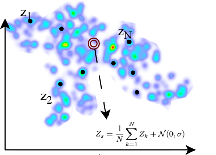
Because the proposed bottleneck latent space is not forced to have a prior distribution shape (for the sake of better reconstruction), we follow a straightforward bootstrap aggregating technique. Figure 2 illustrates the $k$-sample latent space vector averaging pipeline, and Eq. (2) formalizes sampling process. To introduce controlled diversity while preserving station characteristics, we average $N$ (selected as 5 in our experiments) encoder features (i.e. latent codes) from the a specific station record pool and decode the mixed representation under the target station label. We also add Gaussian noise with standard deviation $\sigma$, where $\sigma$ is computed from the latent codes of all records belonging to a specific station.

$$Z_{s}=\frac{1}{N}\sum_{k=1}^{N}Z_{k}+\mathcal{N}(0,\sigma)$$ (1)

Figure 2: TimesNet-Gen sampling via $k$-sample encoder-feature averaging within a station pool.

Since the $N$ latent codes are randomly sampled from the station-specific latent pool at each generation step, the resulting latent representation varies across different sampling instances. The random selection of latent codes, together with the additive Gaussian perturbation, introduces stochasticity into the generation process. As a result, each sampling step produces slightly different realizations while still reflecting the statistical characteristics of the station-specific records. In this way, the proposed procedure generates diverse samples consistent with the underlying distribution of the station data rather than deterministically interpolating between a fixed set of latent vectors.

II-B Variational Autoencoders

Variational Autoencoders (VAEs) [10] are generative models that learn a probabilistic mapping between observed data and a lower-dimensional latent space. They consist of an encoder and a decoder that compress and reconstruct the data, enabling the generation of new samples. The proposed variational autoencoder consists of a convolutional encoder and a symmetric deconvolutional decoder. The encoder employs four consecutive convolutional layers with $3\times 3$ kernels and Leaky ReLU activations, followed by a flattening operation and two linear layers that produce the latent mean and standard deviation parameters. Latent variables are sampled using the reparameterization trick and passed to the decoder, which begins with a linear transformation and reshaping step. The decoder comprises four transposed convolutional layers with $3\times 3$ kernels and Leaky ReLU activations, concluding with a sigmoid output layer that reconstructs the input.

1) Latent Space Conditioning: To incorporate station information into the generative process, similarly to the TimesNet-Gen, the VAE is conditioned in the second training phase. The conditioning is done only in the second training phase and for the VAE, this second training phase, includes two separate conditioning sub-phases. In the first sub-phase, the model is conditioned using one-hot encoded class priors. Each class is assigned a distinct prior mean vector $\mu_{p}$ constructed by tiling one-hot encodings across the latent dimensions, while the prior variance is fixed to $\sigma_{p}^{2}=1$. To ensure separable priors, the latent dimension is chosen as a multiple of the number of classes (five in this case), resulting in a 510-dimensional latent space. The Kullback–Leibler divergence term used in the loss is computed as

$$\mathrm{KL}(q(z\mid c)\,\|\,p(z\mid c))=\frac{1}{2}\sum\Big( \frac{\sigma_{q}^{2}}{\sigma_{p}^{2}}+\frac{(\mu_{q}-\mu_{p})^{2}}{\sigma_{p}^{2}}$$ (2)

$$-1-\log\frac{\sigma_{q}^{2}}{\sigma_{p}^{2}}\Big)$$

where $\mu_{q}$ and $\sigma_{q}^{2}$ denote the encoder-predicted mean and variance, respectively, and $(\mu_{p},\sigma_{p}^{2})$ correspond to the parameters of the class-specific prior distribution. Here, $p(z\mid c)$ represents the class-conditioned prior.

In the second phase, the latent space is further refined to sharpen the class clusters, following the approach of Mousavi et al. [20]. Encoded representations $z_{i}$ are obtained from the first phase, and initial cluster centers $\mu_{j}$ are computed as the mean of samples belonging to each class. Cluster membership probabilities are estimated as

$$q_{ij}=\frac{(1+\|z_{i}-\mu_{j}\|^{2})^{-1}}{\sum_{j}(1+\|z_{i}-\mu_{j}\|^{2})^{-1}},$$ (3)

and a sharpened target distribution is defined as

$$p_{ij}=\frac{\frac{q_{ij}^{2}}{\sum_{i}q_{ij}}}{\sum_{j}\left(\frac{q_{ij}^{2}}{\sum_{i}q_{ij}}\right)}.$$ (4)

The clustering loss is given by the Kullback–Leibler divergence between the sharpened and soft assignment distributions,

$$\mathcal{L}_{c}=\mathrm{KL}(P\|Q)=\sum_{i}\sum_{j}p_{ij}\log\left(\frac{p_{ij}}{q_{ij}}\right),$$ (5)

and is added to the original VAE objective with a weighting factor $a$ (100 in our experiments), yielding the final loss function

$$\mathcal{L}_{\text{final}}=\mathcal{L}_{\text{VAE}}+a\,\mathcal{L}_{c}.$$ (6)

2) Input Preprocessing: The aim of these preprocessing steps is to ensure that both amplitude and phase information can be effectively learned by the model while preserving the essential structural characteristics of the signal. In the preprocessing pipeline, spectrograms containing both amplitude and phase information were generated for each seismic record. First, short-time Fourier transform (STFT) is applied to all three channels of each record to produce amplitude and phase spectrograms, resulting in a multi-channel representation for each recording. The amplitude spectrograms are then converted to a logarithmic decibel (dB) scale to make them more perceptually meaningful and to facilitate the learning process. Phase spectrograms, initially obtained as wrapped phases within the range of -$\pi$ to $\pi$ due to the FFT, exhibited discontinuities along the time axis; these are corrected using phase unwrapping to produce a continuous and smooth phase profile.

In order to be able to evaluate the results and compare them to TimesNet-Gen outputs, the spectrograms are converted back to time-domain signals. This was achieved by first denormalizing the amplitude and phase spectrograms, transforming the amplitude spectrograms from the logarithmic scale back to linear values, and then combining the amplitude and phase components before applying the inverse short-time Fourier transform.

II-C Dataset

In our experiments, we employ strong-motion recordings from the Disaster and Emergency Management Presidency of Türkiye (AFAD) database [27] (36,417 records, 2012–2018). As explained in the following subsection we utilize two separate sets in order to adopt a two-phase training schedule. The first phase of training utilizes an unsupervised pretraining scheme on the entire corpus, followed by the second phase, where the models are fine-tuned on records collected from five stations (a total of 348 records that were not included in the first phase) for station-conditioned generation. While selecting these stations, our criterion was finding stations with different site properties to test the generative model’s ability to generate distinct classes. Hence, we chose five stations with different fundamental site frequencies. Some of the fundamental frequencies reported here (specifically for stations 2020 and 0205) differ from what is reported in AFAD website due to differences in the calculation method. Fundamental site frequency is typically calculated empirically from the horizontal-to-vertical spectral ratio (HVSR) analysis of ambient recordings [21] as well as earthquake recordings [13] [31]. In this study we compute based on using strong motions signals, [13] [31]. The five stations used in this study and their identified fundamental frequencies are given in Table I.

TABLE I: Properties of the Selected Stations

Station Id	Location	$f_{0}$	No. of rec.
2020	Tavas / Denizli	5.1 Hz	71
4628	Afsin / Kahramanmaras	1.8 Hz	38
0205	Kahta / Adiyaman	2.6 Hz	98
1716	Ayvacik / Canakkale	6.4 Hz	110
3130	Defne / Hatay	12.8 Hz	31

II-D Two-Phase Training

Both models are trained with a two-phase strategy. Models are first trained in an unsupervised manner with no conditioning, so as to construct a base latent code space. In the second phase, we fine-tune the model with station conditioning while injecting controlled Gaussian noise based on the stored standard deviations.

For both models the conditioning information is not introduced in the first training phase. Phase 0 is primarily used to learn the latent representation and to obtain statistical properties of the encoder features. In the second phase, station-specific conditioning is applied according to each method’s strategy. For cross-validation purposes, the 348 records from the selected stations used in fine-tuning are excluded from the first-phase training.

To assess whether TimesNet-Gen’s station-specific performance stems from explicit station conditioning (via station ID) or from its sampling strategy (selecting samples from the same station), an additional experiment was conducted. A single-phase, fully unsupervised TimesNet-Gen model was trained without any station conditioning, and generation for the five target stations was performed in a zero-shot manner by feeding only their waveforms to the encoder. The results remained consistent with the two-phase conditioned approach, indicating that the model’s ability to capture station characteristics is not derived from explicit station ID embedding, but rather from the learned latent representations based on waveform features alone. This suggests that the latent representations naturally encode site-specific response properties in an unsupervised manner, and the station-specific sampling strategy effectively leverages this implicit clustering.

II-E Evaluation

To analyze the generation quality, two methods: a spectral- and the proposed distribution-based metric are used.

1) Spectral Analysis: The characteristics of earthquake recordings depend on several factors, including source, path, and site effects [12]. One key site effect is the modification and amplification of ground motions through resonance, which occurs when incoming seismic waves contain energy close to the site frequency. The fundamental site frequency ($f_{0}$) is a critical parameter that represents site response and depends on the thickness and properties of the underlying soil layer. As stated earlier we use strong motion signals recorded at the sites to calculate ($f_{0}$). The calculation procedure is summarized below.

Horizontal-to-vertical spectral ratio (HVSR) curves are calculated using signals recorded from three channels: north-south ($H_{1}(t)$), east-west ($H_{2}(t)$), and vertical ($V(t)$) at the stations. First, amplitude spectra are calculated, $|H_{1}(f)|$, $|H_{2}(f)|$, and $|V(f)|$, then average horizontal amplitude is found using Eq. 7:

$$|H(f)|=\sqrt{\frac{|H_{1}(f)|^{2}+|H_{2}(f)|^{2}}{2}}$$ (7)

Finally, the HVSR curve is constructed by dividing the average horizontal amplitude by the vertical amplitude spectra for each frequency as in Eq. 8:

$$\text{HVSR}(f)=\frac{|H(f)|}{|V(f)|}$$ (8)

In the HVSR curve, the lowest clear resonance peak is taken as the fundamental site frequency $f_{0}$. Given that seismic waves are significantly amplified at or near the fundamental site frequency, it is critical to design structures with natural frequencies that avoid resonance with the site’s predominant frequency. We restrict our analysis to the 1–20 Hz band and apply the same preprocessing and smoothing across all sources to ensure consistency.

2) $f_{0}$ Distribution Confusion Matrices: To further evaluate the physical consistency of the generated signals, we analyze the distributions of the calculated $f_{0}$ values obtained from both real and model-generated samples, for each station separately. For every $N$ real sample of a station, we first compute the $f_{0}$ distribution. Then, using for both models, we generate and reconstruct same number of synthetic samples per station and extract their corresponding $f_{0}$ values to build comparable distributions.

To quantify the similarity between these distributions, we employ the Jensen–Shannon Divergence (JSD). Since JSD measures dissimilarity, we convert it into a similarity score by taking its complement (i.e. 1 indicates perfect similarity, whereas 0 indicate no similarity). Next, we compute the intercorrelations for each station separately and filled them into a matrix. In this matrix, we expect the signals from the same station (real vs. TimesNet-generated vs. VAE-generated) to yield high similarity scores, while signals from different stations should produce low similarity scores, for each real vs. TimesNet-generated vs. VAE. The resulting 15x15 matrix corresponds to 5 stations (2020, 0205, 4628, 1716, 3130) × 3 signal types (real, generated, reconstructed) and is specific to each model.

To evaluate the overall quality of each method, we calculated the distance between our matrices and an ideal matrix (each diagonal block corresponds to a station (3×3) with all entries set to 1, and all inter-station elements are 0) using Normalized Cross-Correlation (NCC). Related figures can be found in the Results section.

III Experiments and Results

III-A Sample Results

Figure 3: t-SNE projection of the latent space for station 1716.

We first visualize the structure of the latent space. t-SNE (t-distributed Stochastic Neighbor Embedding) is a method that reduces high-dimensional data to two or three dimensions while preserving local similarities. Figure 3 shows a two–dimensional t-SNE projection of the latent representations for station 1716. Black points correspond to latent vectors obtained from real records (latent bank), while blue points denote latent samples generated during the sampling process by uniformly interpolating between latent vectors from the latent bank. This projection indicates that the latent space forms a continuous structure rather than isolated clusters; this demonstrates that the model effectively captures the variations in the seismic signals.

We then visually analyze some generated signals for each model. As seen in Figure 4, real and TimesNet-Gen generated sample E-W components exhibit earthquakes with varying durations and amplitudes. The bottom figures are the corresponding Fourier amplitude spectra, showing frequency behaviour similar to real samples.

In the following, we focus on general spectral and frequency-domain evaluations and assess how well each model captures station-dependent frequency content, dominant site frequencies, and overall HVSR behavior.

Figure 4: Real and TimesNet-Gen generated samples for three stations with corresponding Fourier amplitude spectra.

III-B Spectral Analysis

For spectral analysis, we first present the $f_{0}$ distributions for real data, each model’s reconstructed samples, and generated samples in Figure 5. We generate 50 samples to create a distribution and present these distributions. We also evaluate ”reconstructed” results, which we obtain by feeding real signals through the encoder–decoder pathway and measuring reconstruction fidelity. In practice, this provides an upper bound on the generative quality we could expect from any sampling strategy. As seen in the figure, TimesNet performs better, with reconstruction quality remaining largely consistent across stations, whereas it degrades considerably for the VAE. TimesNet generates samples that follow the real $f_{0}$ distributions more closely, including at stations where the empirical distribution shows irregular or wide-spread behavior. In addition, its performance remains stable across different frequency ranges, indicating that the model captures station-specific spectral patterns more reliably.

(a) Station 0205

(b) Station 1716

(c) Station 2020

(d) Station 3130

(e) Station 4628

Figure 5: $f_{0}$ distributions for selected stations.

Then, we analyse the average HVSR (average of all individual HVSR curves for a given category) plots separately for real data, each model’s reconstructed samples, and generated samples, in Figure 6. Results show that TimeNet-Gen demonstrates strong performance, even in stations 0205 and 4628, where it is able to capture the peak behavior of each individual HVSR curve. In contrast, VAE tends to deviate either above or below the actual peaks in most cases, and notably at station 0205, it fails to reproduce the sharp peak characteristics. These average distributions provide insight into the models’ ability to preserve site-specific frequency content. When different HVSR curves show consistent peak frequency and amplitude, they capture stable resonance characteristics of the site, emphasizing the need to represent these peaks accurately.

(a) Station 0205

(b) Station 1716

(c) Station 2020

(d) Station 3130

(e) Station 4628

Figure 6: Average HVSR curves for selected stations.

III-C $f_{0}$ Distribution Confusion Matrices

Finally, we calculate the $f_{0}$ Distribution Confusion Matrices for each model, to evaluate the interstation discrimination and real vs model similarity. For each model separately in Figure 7, two 15$\times$15 confusion matrices are provided. As seen from the figure, some stations (most notably 0205 and 4628) have close $f_{0}$ values, as also shown in Table I and Figure 7. A similar pattern is observed for stations 1716 and 2020, which also share comparable $f_{0}$ characteristics. Although close $f_{0}$ values reflect comparable dominant resonance frequencies, they do not fully describe overall site response, which can still differ across stations. Importantly, TimesNet-Gen distinguishes these stations despite their $f_{0}$ proximity, suggesting that the model captures additional waveform characteristics beyond the fundamental resonance alone. In contrast, the VAE baseline shows more ambiguity in these station pairs, with noticeably weaker separation and a tendency to mix stations that share similar $f_{0}$ values.

(a) TimesNet-Gen (alignment score: 0.93)

(b) VAE (alignment score: 0.81)

Figure 7: $f_{0}$ distribution Confusion Matrices for the two models.

IV Conclusions

In this work, we introduce TimesNet-Gen, a station-conditioned, time-domain deep learning model designed to generate realistic site-specific strong motion records. Our approach directly learns from seismic recordings, without relying on traditional ground-motion equations. We evaluate the model using $f_{0}$ distribution confusion matrices and median HVSR curves, demonstrating that TimesNet-Gen can reproduce both spectral and temporal characteristics observed in real recordings. Across multiple stations, the model captures key site-specific features, generating diverse yet physically plausible waveforms that align closely with real data.

Station-wise comparisons further support this observation. Median HVSR curves and $f_{0}$ distributions for TimesNet-Gen closely match real data across all five stations, showing tighter clustering and more consistent amplification patterns compared to VAE. HVSR curves, computed as the ratio of horizontal-to-vertical spectral amplitudes, exhibit similar character. Importantly, the VAE baseline we used was not a randomly selected or an arbitrary model; we explored multiple approaches to shape its latent space and reported the best-performing results as our baseline.

Upon examining our results, we observe that when conditioned on the same station ID, TimesNet-Gen generates waveforms with varying P and S-wave arrival times, amplitudes, and durations. Such variability is consistent with what occurs at a given site due to differences in earthquake sources and propagation paths, and the model reproduces this diversity without converging to a single waveform pattern. In this study, we conduct a frequency-based analysis of these diverse generations. To further enhance the quality of the generated waveforms, future work will include the distributions of P and S wave arrival times, peak ground acceleration, duration, and other intensity related parameters into the evaluation process. Building on this, TimesNet-Gen demonstrates strong potential for additional research directions: the model can be extended toward physics-guided or simulation-oriented earthquake generation, and its encoder’s generalizable representations provide a foundation for downstream seismic tasks such as phase picking, ground-motion parameter estimation, or event classification.

V Acknowledgements

This study was supported by the Middle East Technical University (METU) Scientific Research Projects (BAP) under grant number ADEP-704-2024-11482.

References

- [1] (1992) A stable algorithm for regression analyses using the random effects model. Bulletin of the Seismological Society of America 82 (1), pp. 505–510. Cited by: §I-A, §I.
- [2] (2020) Strong ground motion simulation techniques—a review in world context. Arabian Journal of Geosciences 13 (14), pp. 673. Cited by: §I-A, §I.
- [3] (2024) High resolution seismic waveform generation using denoising diffusion. External Links: 2410.19343, Link Cited by: §I-A, §I-A.
- [4] (2025) Exploring challenges in deep learning of single-station ground motion records. External Links: 2403.07569, Link Cited by: §I.
- [5] (2017) Stochastic ground motion simulation of the 2016 meinong, taiwan earthquake. Earth, Planets and Space 69 (1), pp. 62. Cited by: §I-A.
- [6] (2020) Data-driven accelerogram synthesis using deep generative models. External Links: 2011.09038, Link Cited by: §I.
- [7] (2017) GANs trained by a two time‑scale update rule converge to a local nash equilibrium. In NIPS, pp. 6626–6637. Cited by: §I-A.
- [8] (1981) Peak horizontal acceleration and velocity from strong-motion records including records from the 1979 imperial valley, california, earthquake. Bulletin of the seismological Society of America 71 (6), pp. 2011–2038. Cited by: §I-A, §I.
- [9] (2025) Broadband ground motion synthesis by diffusion model with minimal condition. External Links: 2412.17333, Link Cited by: §I-A, §I-A.
- [10] (2013) Auto-encoding variational bayes. External Links: 1312.6114, Link Cited by: §II-B.
- [11] (2019) An introduction to variational autoencoders. Foundations and Trends in Machine Learning. External Links: Link Cited by: §I.
- [12] (2024) Geotechnical earthquake engineering. CRC Press. Cited by: §II-E.
- [13] (1993) Site effect evaluation using spectral ratios with only one station. Bulletin of the seismological society of America 83 (5), pp. 1574–1594. Cited by: §II-C.
- [14] (2020) Seismic labeled data expansion using variational autoencoders. Artificial Intelligence in Geosciences 1, pp. 24–30. Cited by: §I-A.
- [15] (2020) Seismic data augmentation based on conditional generative adversarial networks. Sensors 20 (23), pp. 6850. Cited by: §I-A, §I-A.
- [16] (2004) ROUGE: a package for automatic evaluation of summaries. In Proc. ACL Workshop on Text Summarization Branches Out, pp. 10. Cited by: §I-A.
- [17] (2010) Hybrid broadband ground-motion simulations: combining long-period deterministic synthetics with high-frequency multiple s-to-s backscattering. Bulletin of the Seismological Society of America 100 (5A), pp. 2124–2142. Cited by: §I-A, §I.
- [18] (2024) Generative adversarial networks-based ground-motion model for crustal earthquakes in japan considering detailed site conditions. Bulletin of the Seismological Society of America 114 (6), pp. 2886–2911. Cited by: §I-A.
- [19] (2020-11) Bayesian-deep-learning estimation of earthquake location from single-station observations. IEEE Transactions on Geoscience and Remote Sensing 58 (11), pp. 8211–8224. External Links: ISSN 1558-0644, Link, Document Cited by: §I.
- [20] (2019) Unsupervised clustering of seismic signals using deep convolutional autoencoders. IEEE Geoscience and Remote Sensing Letters 16 (11), pp. 1693–1697. External Links: Document Cited by: §II-B.
- [21] (1989) A method for dynamic characteristics estimation of subsurface using microtremor on the ground surface. Railway Technical Research Institute, Quarterly Reports 30 (1). Cited by: §II-C.
- [22] (2022) A time series is worth 64 words: long-term forecasting with transformers. arXiv preprint arXiv:2211.14730. Cited by: §I.
- [23] (2025) Two years on: a look at undp’s earthquake recovery efforts in türkiye. Note: https://www.undp.org/turkiye/news/two-years-look-undps-earthquake-recovery-efforts-turkiyeAccessed: 2025-09-20 Cited by: §I.
- [24] (2024) Learning physics for unveiling hidden earthquake ground motions via conditional generative modeling. External Links: 2407.15089, Link Cited by: §I-A.
- [25] (2024) Findings from a decade of ground motion simulation validation research and a path forward. Earthquake Spectra 40 (1), pp. 346–378. External Links: Document, Link Cited by: §I-A.
- [26] (2024) Broadband ground-motion synthesis via generative adversarial neural operators: development and validation. Bulletin of the Seismological Society of America 114 (4), pp. 2151–2171. Cited by: §I-A.
- [27] (2024) Deep learning-based epicenter localization using single-station strong motion records. External Links: 2405.18451, Link Cited by: §I, §II-C.
- [28] (2024) Timemixer: decomposable multiscale mixing for time series forecasting. arXiv preprint arXiv:2405.14616. Cited by: §I.
- [29] (2023) TimesNet: temporal 2d-variation modeling for general time series analysis. External Links: 2210.02186, Link Cited by: §I, §II-A.
- [30] (2024) Site-specific ground-motion waveform generation using a conditional generative adversarial network and generalized inversion technique. Bulletin of the Seismological Society of America 114 (4), pp. 2118–2137. Cited by: §I-A, §I-A.
- [31] (2022) A new set of automated methodologies for estimating site fundamental frequency and its uncertainty using horizontal-to-vertical spectral ratio curves. Seismological Society of America 93 (3), pp. 1721–1736. Cited by: §II-C.
- [32] (2024) Deep learning-based average shear wave velocity prediction using accelerometer records. External Links: 2408.14962, Link Cited by: §I.