A Modular Architecture Design for Autonomous Driving Racing in Controlled Environments
Abstract
This paper presents a modular autonomous driving architecture for Formula Student Driverless competition vehicles operating in closed-circuit environments. The perception module employs YOLOv11 for real-time traffic cone detection, achieving 0.93 mAP@0.5 on the FSOCO dataset, combined with neural stereo depth estimation from a ZED 2i camera for 3D cone localization with sub-0.5 m median error at distances up to 7 m. State estimation fuses RTK-GNSS positioning and IMU measurements through an Extended Kalman Filter (EKF) based on a kinematic bicycle model, achieving centimeter-level localization accuracy with a 12 cm improvement over raw GNSS. Path planning computes the racing line via cubic spline interpolation on ordered track boundaries and assigns speed profiles constrained by curvature and vehicle dynamics. A regulated pure pursuit controller tracks the planned trajectory with a dynamic lookahead parameterized by speed error. The complete pipeline is implemented as a modular ROS 2 architecture on an NVIDIA Jetson Orin NX platform, with each subsystem deployed as independent nodes communicating through a dual-computer configuration. Experimental validation combines real-world sensor evaluation with simulation-based end-to-end testing, where realistic sensor error distributions are injected to assess system-level performance under representative conditions.
I Introduction
Autonomous vehicle systems in controlled environments present significant challenges in integrating multiple subsystems for real-time navigation and decision-making. The development of modular architectures that effectively combine perception, localization, path planning, and control systems represents a critical area of research in autonomous driving technology. This work presents a comprehensive framework for the connectivity and allocation of responsibilities within an autonomous driving architecture, focusing on precise operation in closed-circuit scenarios. The approach defines four primary modules: perception, localization and mapping, trajectory planning, and control. It also describes their interconnection through a communication pipeline. The paper also reviews the current state of the art, analyzes the main technological advances, and justifies the design choices made to address the scientific and engineering challenges faced by autonomous vehicles in constrained, competitive or experimental environments.
II Autonomous Vehicle System Overview
The architecture of an autonomous vehicle is a particular implementation of a more generic control system. Therefore, the classic components of sensors, actuators, controller, and plant must be reinterpreted and mapped to the autonomous driving ecosystem. Figure 1 shows a simplified version of this projection. The sensors are mainly a vision system, an IMU (Inertial Measurement Unit), and a positioning system. The actuators are concentrated into an ECU (Electronic Control Unit) system, which translates the commands received by the controller into direct actions on the steering wheel, accelerator, and brake systems. The controller is the autonomous system itself, which computes at each iteration a new reference (velocity) based on a path planning algorithm and compares it with the received position, video, and IMU data, constituting the SLAM (Simultaneous Localization and Mapping) system.

II-A Hardware Components
II-A1 Control System
The Control System of the Autonomous System (AS) is suitable to be implemented entirely on an On-Board-Computer. The On-Board-Computer has to have quite high computing capabilities in order to solve in real time several complex calculations like integration of positioning, IMU and Vision systems into an Extended Kalman Filter (EKF), and the use of several AI (Artificial Intelligence) algorithms.
II-A2 Sensors
The data generated by the sensors serves as input to the Control System in order to be compared with the desired reference. The sensors are installed to determine the behavior of the vehicle, and particularly its absolute or relative position within a defined area.
-
•
Position sensors. These sensors help the vehicle understand its coordinates and orientation relative to the environment. The most used ones are GNSS (Global Navigation Satelite Systems), LiDAR (Light Detection and Ranging), GSS (Ground Speed Sensors), odometry sensors (encoders), IMU among others.
-
•
Vision sensors. Image processing has become an important source of data for obstacle detection and environmental interpretation. Mono and stereo cameras complemented with image processing software generates useful control input data.
-
•
Odometry. Motor position encoders are suitable for accurate short-distance travel. Steering angle and wheel encoders are examples for that.
-
•
Cinematic. Torque and acceleration data are provided by IMU in order to detect rapid behavior changes.
II-A3 Actuators
Actuators are mainly concentrated into three components: the throttle actuator, the steering system and the brake system. Usually, the output of the Control System is an acceleration vector. Nevertheless, this acceleration is translated into the steering system, the linear acceleration and the brake system. Usually, in a vehicle, these actuators are connected using field bus technologies such as CAN bus, where the communication is controlled by an Electronic Control Unit (ECU).
II-A4 In Vehicle Communications
Data transmission between the components of the vehicle is based on the Controller Area Network (CAN) protocol [7]. Usually, the interface adheres to a specific software specification depending on the vehicle.
II-B Software
The software components bind all the data generated and needed by the hardware components together. The On-Board computer that hosts the Control System has to process the inputs that come from the sensors, generate the outputs, and send them to the actuators. Therefore, the On-Board computer hosts the most important part of the software components.
III Implementation
The presented AS is developed to compete in the Formula Student Driverless competition [6], and was deployed at Formula Student UK (FSUK) at Silverstone Circuit. The competition organizers provide an electric car with all actuators integrated in a Vehicle Control Unit (VCU) connected to an In-Car-PC equipped with Ethernet and CANBus interfaces. The interface adheres to the AS-DV software specification defined for the competition [5], categorizing messages into control commands, sensor feedback, and mission status flags. The Control System is hosted by an On-Board computer; therefore, this architecture is called a dual-computer architecture (On-Board-Computer and In-Car-PC). The circuit is delimited by two sets of cones: blue cones for left track limits and yellow cones for right track limits, with large orange cones marking the start and finish lines. This requires an object detection system to be integrated into the AS.
III-A Selected Hardware Components
The main hardware components are the On-board computer that hosts the Control System and the position and vision sensors. As position sensor, the authors propose a Real-Time-Kinematic (RTK) system in order to improve classical GNSS data and as vision sensor a stereo camera in order to facilitate the calculation of depth and positioning relative to the location of the cones.
The whole hardware architecture (dual-computer architecture) consists of five primary components: a ZED 2i stereo camera, a simpleRTK2B receiver, a reComputer-based On-Board-Computer (primary AS host), a dedicated In-Car-PC (secondary computer for CAN communication), and the VCU. The On-Board-Computer executes all perception, planning, and control modules, while the in-car PC handles CAN Bus communication and the interface with the Vehicle Control Unit. This separation ensures that computationally intensive algorithms run independently from real-time communication interfaces. The hardware components and the connectivity are shown in figure 2.

III-A1 On-board computer
The Control System of the AS runs on a reComputer J4012 powered by the NVIDIA®Jetson Orin NX module [14]. This System-on-Module (SoM) features an integrated Ampere GPU with 1024 CUDA cores and dual deep learning accelerators, delivering up to 100 TOPS of AI performance for the vision pipeline. The system operates on Ubuntu 20.04 with ROS 2 Galactic, utilizing the architecture described by Macenski et al. [13]. The middleware is virtualized via Docker to ensure compatibility, while the in-car PC runs Ubuntu 22.04 with ROS 2 Humble.
III-A2 Real-time kinematic positioning
The simpleRTK2B module from ArduSimple [3] provides centimeter-level GNSS accuracy. It utilizes the u-blox ZED-F9P multiband GNSS engine to receive corrections from a fixed base station up to 11 km away. The rover board computes Real-Time Kinematic (RTK) solutions at a rate of 10 Hz, providing the high-precision absolute positioning required for the Extended Kalman filter updates.
III-A3 Stereo camera
The ZED 2i [20] captures 1920x1080 stereo images at 30fps with a 120º field of view. It integrates a 9-DOF IMU (accelerometer, gyroscope, and magnetometer) running at 400 Hz, which is factory-calibrated and synchronized with the video stream. Its IP66-rated enclosure ensures reliability during adverse weather conditions typically encountered in competition.
III-B Software components
The On-board computer hosts the whole Control System of the AS. Communications with the other components are done by the parametrization and correct use of the operational drivers of the sensors and actuators.
The AS is developed on ROS2 [17], a software framework that provides utilities for complex robotic machines. Each module is implemented via a ROS2 package and each submodule is implemented via ROS2 nodes as illustrated in Figure 3.

III-C Computer Vision
The main objective of the computer vision module is to take camera images and process them in order to detect the cones that delimit the track. The object detection and depth calculation nodes take left and right images from the camera driver. A computer vision model is used to detect the cones delimiting the track, while a depth calculating algorithm calculates a depth image. Using both the detections and the depth information, the positioning node calculates a bird’s eye view positioning of the cones relative to the car. The nodes that are part of the computer vision module are marked in red in the figure 3.
III-C1 Depth calculation
Stereolabs offers as part of their SDK for the ZED a depth calculation functionality [19]. It allows a variety of depth calculation modes, that change the performance and speed of the calculation. During our experiments, the best results were obtained by using the Neural mode. This mode uses an end to end AI powered calculation. This calculation is very computer intensive and uses the API for parallel computing CUDA to compute the depth in the reComputer. The use of a visual tracker, combined with the mapping algorithm mitigates the depth error.
III-C2 Object Detector
For object detection (cones) the version 11 of the open source YOLO product from Ultralytics is selected [21].
YOLOv11 [8] was released in September 2024 by Ultralytics [1]. There are some pre-prints that analyse the performance of the YOLOv11 model [21]. In these pre-prints the YOLOv11 model performed better than its predecessors in speed and accuracy. For these reasons, YOLOv11 was chosen as the detection model.
Ultralytics offers different pretrained models to use as training baseline. The YOLOv11 model chosen was the YOLOv11s object detection model, since in our experiments the accuracy difference between the ’s’ and ’m’ models was not significant, while the speed difference was noticeable.
THe YOLO solution has to be trained using a dataset. The FSOCO dataset was used to train the model [22]. The best results were obtained at around 40 iterations and further training seemed to cause overfitting. To search the best combination for the 30 hyperparameters a genetic algorithm was used to optimize a fitness function defined as follows:
| (1) |
The fitness function defined in Equation 1 assigns the dominant weight (0.8) to mAP50:95, which evaluates detection accuracy across IoU thresholds from 0.50 to 0.95 in steps of 0.05, penalizing detections with imprecise bounding boxes. Recall and mAP50 each contribute 0.1, ensuring that the optimization does not sacrifice detection completeness or baseline localization quality. This weighting reflects the priority of tight spatial accuracy over mere detection presence, which is critical for downstream cone positioning: a detection that loosely overlaps a cone may count as correct at IoU 0.50 but fail at stricter thresholds, propagating localization error into the mapping and path planning modules. The genetic algorithm optimizes this function using a 90 percent mutation probability with 0.04 variation to generate new candidates from the best-performing parents of previous generations.
III-C3 Object tracker
A multi object tracker (MOT) is an algorithm that allows recovering the identity information of several detected object across frames [12]. In the presented design an object tracker is used to maintain the cone identities across time. Since the mapping algorithm will also provide a way to identify the cones, there is no need to have a highly precise tracker, therefore it was chosen the Intersection-Over-Union (IOU).
The method assumes that an object detector produces a detection per frame for every object to be tracked. It also assumes that consecutive detections of an object have a high overlap IOU, which is true in sufficiently high frame rates. The IOU measure can be defined using the equation 2.
| (2) |
When both requirements are met, tracking with this method can be done without using any image information. The tracker continues the identity by associating the detection with the highest IOU to the last detection in the previous frame if a certain threshold is met [4]. All detections not assigned to an existing track will start a new one. All tracks without an assigned detection will end.
III-C4 Cone positioning
The 2D positioning is calculated using both the detected images and the depth information. The position was modeled using a distortion-free projective transformation given a pinhole camera model following Equation 3.
| (3) |
Where is a 3D point expressed with respect to world coordinates, is a 2D pixel in the image plane, is the camera intrinsic matrix, and are the rotation and translation that describe the change of world coordinates to camera coordinate systems, and is the projective transformation’s arbitrary scaling and not part of the camera model [15]. The camera intrinsic matrix is composed of the lengths expressed in pixel units () and the principal point () following the equation 4.
| (4) |
The world coordinates are equal to the camera coordinates since the translation and rotation will be calculated in the mapping node. Therefore, the rotation and translation matrix is the identity . This model allows to calculate the image projected given the real coordinates. The depth information can be used to calculate the z given the camera intrinsic parameters and the pixel position using similar triangles.
III-D Positioning and mapping
The Positioning and Mapping module captures sensor data to determine accurate location and orientation. It consists of the submodules Camera Driver, RTK Driver, Extended Kalman Filter, Mapping, and Map Awareness. RTK and IMU data are the main inputs, which are combined using a Extended Kalman Filter to achieve high accuracy. The Mapping submodule creates a global map of the circuit by combining location and computer vision data, assigning a linear order to cones and publishing the car’s position and map information. Additionally, the map awareness node provides information about the car’s position on the track.
III-D1 Extended Kalman Filter
A Kalman filter [10] is an algorithm that uses a series of measurements observed over time to produce estimates of unknown variables. The algorithm works in a two-phase process: predict and update. In the prediction phase, the filter estimates the current state variables and uncertainties. In the update phase, these estimates are corrected using a weighted average of the new measurements, prioritizing those with greater certainty.
In the context of autonomous racing, state estimation typically relies on fusing high-frequency ego sensors (IMU, odometry) with positioning systems (GNSS-RTK). For this architecture, we employ the Kinematic Bicycle/Tricycle Models as the dynamical system foundation. These models are widely validated in closed circuit racing operations [9], [16] for their optimal balance between computational load and prediction accuracy.
While dynamic models account for complex tire-slip mechanics, the kinematic approach fused with GNSS updates has been proven to maintain decimeter-level accuracy ( cm) in dynamic environments [2]. Furthermore, recent experimental comparisons demonstrate that EKF fusion using this modeling approach can improve localization accuracy by approximately 32% compared to raw sensor data [11], therefore it’s selected for achieving the 1-2 cm target accuracy when combined with RTK corrections.
The control system outputs are the longitudinal acceleration and the steering angle , and the inputs are the GNSS coordinates , the magnetometer heading angle , the vehicle speed (median of rear wheel speeds), and the IMU angular velocity , as shown in Figure 4.

To model the system, it is required to represent a linear system using a propagation model (equation 5) and a measuring model (equation 6).
| (5) | ||||
| (6) |
Where is the current instant, is the internal state vector, is the input vector, is the output vector, , and are the model matrices, and and are the considered errors. The internal state vector is composed of the and coordinates, the turning angle and the vehicle speed .
Our approach used a uniformly accelerated rectilinear motion (UARM) to calculate , and (equations 7, 8 and 9). And lastly for the speed we simply develop the acceleration formula (equation 10).
| (7) | |||||
| (8) | |||||
| (9) | |||||
| (10) |
Where is the sampling period. With a sampling period small enough, the last component of equations 7, 8 and 9 will be much smaller than the other components, so it can be ignored to simplify the model. In the design, will be 0.1 seconds, because the RTK has a maximum refresh rate of 10Hz. Developing the above equations, the propagation model will follow the equation 11.
| (11) |
The terms of equation 11 are:
-
•
, : Vehicle position coordinates at time step . These denote the current location of the vehicle in the global (or chosen local) reference frame.
-
•
: Heading angle (orientation) of the vehicle at step , typically in radians.
-
•
: Longitudinal velocity (speed) of the vehicle at time .
-
•
: Sampling interval, i.e., the time difference between steps and (in seconds).
-
•
: Steering angle at time step , representing the front wheel’s angular deviation from the forward direction.
-
•
: Wheelbase, that is, the distance between the front and rear axles of the vehicle.
-
•
: Longitudinal acceleration applied at time .
Each row of the propagation equation gives the predicted value at the next step (), given the current state and applied control input:
-
•
: Next x-position, determined by forward motion and heading.
-
•
: Next y-position, following a similar principle.
-
•
: Updated heading angle, proportional to current turning rate.
-
•
: Updated speed, incremented by the product of acceleration and sampling time.
Equation 11 can be reformulated in equation 12 in order to match the state equations of the model (equations 5 and 6) and identify the model matrices.
| (12) |
Where is the error. To estimate the error, a normal distribution centered at 0 is assumed, where the covariances are our estimation of the maximum possible error (equation 13). A diagonal covariance matrix is used since it is assumed that the errors in each internal state are uncorrelated. The values given as covariance in the matrix are estimated based on the specifications of the actuators.
| (13) |
Where is a function that returns a square diagonal matrix with the elements of vector on the main diagonal. With equations 12 and 13 the propagation model defined in equation 5 is specified. To specify the measuring model (equation 6), we need to correlate the internal state with the outputs and add the error, as per equation 14.
| (14) |
Where the error vector is approximated using a normal distribution, mean 0 and covariance the estimated maximum error, following equation 15. In a similar fashion as equation 13 it is assumed that the errors are uncorrelated so a diagonal matrix is used. The values given as covariance in matrix are estimated based on the specifications of the sensors.
| (15) |
Therefore, the model for the Extended Kalman filter is defined using equation 12 with error 13 in the propagation step and equation 14 with error 15 for the measuring step.
III-D2 Mapping
The mapping node stores the cone and car positions across time. It uses the first values received by the Extended Kalman Filter as the world reference coordinates. From that point onward, all the coordinate information received will be transformed relative to that reference. The mapping node continuously receives the cone position and identity over time. To avoid the identiy switch errors, whenever the mapping node receives a new identity, it checks an oval area across the nearest cone. If the new detection is within this area, it is considered to be the same cone and it updates the new position to a weighted average of all the detections assigned to that cone. To calculate the average, the coefficient is inversely proportional to the distance, so the nearer cones weigh more than the farther ones. this mitigates the error generated by the depth camera. Since the search area changes inversely proportional with the distance, the nearest cones have a smaller search area than the farther ones. The mapping node publishes the cones currently visible, and all the cones detected so far. These cones must be ordered so the path-planning algorithm works properly. To order the cones an algorithm is used that searches in a triangular area following the vector defined by the previous cone of the same color as represented in figure 5.

To define the beginning of either side of the track, the algorithm looks for the orange cones indicating the start line that are closest to the first blue/yellow cones of the track. The triangular search area varies depending on the mission. If several cones are detected in the area, the closest one to the previous cone will be the next counted one. If a detected cone does not fall in any search area, it is considered not relevant for this section of the track and will be ignored.
III-D3 Map Awareness
The map awareness node uses the mapping and positioning information offered by the mapping node to calculate relevant information about the position of the car in the track. This information differs between missions. The information that this node provides is: the number of laps run, the current kind of lap (recon or timed), whether the finish line has been reached, if the vehicle is near the finish line, and if the vehicle is outside the track limits. In case of the skidpad mission, it also detects when the vehicle is near the skidpad central section, and the number of times it runs across it.
III-E Path Planning
The Path Planning node calculates the position of the car at each moment, using the Spline submodule. The Spline module calculates the middle point of the track by interpolating the cones positions, and segments it into points with designated speeds for the Control node to follow. The racing line is computed as the midline between both track boundaries. First, the left and right track limits are defined by fitting independent 2D cubic splines through the ordered series of blue and yellow cones, respectively. These splines allow densely resampling each boundary at arbitrary resolution. Corresponding points on opposite splines are then paired to form transverse lines across the track, and the midpoint of each transverse line is interpolated to produce the racing line. This line is discretized into a sequence of waypoints for the Pure Pursuit controller to follow. The path planning algorithm operates in two modes. During the discovery lap, the spline is computed using only the currently visible cone detections. Once the system determines that the track forms a closed loop, global path planning activates and recomputes the spline over the entire mapped circuit [18]. For each waypoint along the discretized racing line, the node assigns a target speed constrained by the maximum allowed velocity, the maximum steering angle, and the steering rate, ensuring that the regulated Pure Pursuit controller can track the path at the assigned speeds without exceeding the vehicle’s kinematic limits.
III-F Global Map Alignment
For not closed circuit operations, it is necessary to position the ego vehicle against the defined track. In this kind of mission, it is insufficient to follow the track definition as it is discovered, specially if the track presents some kind of unusual layout definition. In this kind of layout, the pathplanning algorithm is not able to properly calculate a path following the mission rules. To fix these issues, we introduced an alternative pipeline that replaces mapping and pathplanning called Global Map Alignment. In this scenario, the position of the cones is known beforehand, so it is possible to store the position and path of the whole track and load it during the event. The Global Map Alignment node can accurately position the entire track by only seeing the first cones. It achieves this by storing a CSV file containing the position of all cones in the track, and mapping the coordinate frame given by positioning to ground truth using a 2x2 transformation matrix in order to cover rotation and scaling.
When we first detect the orange cones in the beginning of the track, we calculate the transformation matrix:
Where , are the coordinates of the cones from the vision module; and , are the coordinates of the cones in the CSV track.
This is just the basic transformation matrix; it does not necessarily transform all cones accurately, particularly because cones located farther from the start zone are highly sensitive to slight changes in the original input. To address this, we iteratively adjust the transformation matrix by using random numbers, aiming to minimize the following expression:
| (16) |
With defined as the distance from each cone to its predicted position. The fractional part ensures that cones that are closer are prioritized.
III-G Control
The control module moves the vehicle along the calculated path using a Pure Pursuit algorithm. The Pure Pursuit Node calculates the target acceleration, steering and braking based on the path and speed profile from the path planning module, and the current car’s position from the mapping module using a geometric following algorithm.
The pure pursuit algorithm works by defining a circular path that intersects with the spline given by path planning. This intersection defines a lookahead point, that is usually 3-5 seconds distance ahead. We define the acceleration at any given point as the difference between the current speed and the target speed (defined by the speed profile), multiplied by a constant factor of to avoid overshooting. Our implementation is a special case of pure pursuit algorithm called regulated pure pursuit. This algorithm differs from the general pure pursuit algorithm by having a dynamic lookahead that can be parameterized. This lookahead value is then used in the following equation to determine the delta in steering:
| (17) |
Where is defined as the direction to the target point; , as the orientation of the car; , as the change in direction needed; , as the wheelbase of the vehicle; and as the selected lookahead.
The lookahead is selected following the next equation:
| (18) |
Defining and as the lower and higher bounds of the lookahead; and and as the target speed as defined by the speed profile and the current speed.
III-H Master Node
The master node is the system entrypoint. It will manage module activations and the system internal flags. To ensure that the system does not launch any unexpected actuator movements whenever the AS enters the driving status, the master node activates the nodes from the path-planning and control packages. When the AS changes the status to any other, these nodes are deactivated.
The master node checks the mission and the internal state variables provided via the CAN node, and sets a series of parameters to the other nodes. One of these parameters is the flag to set the initial coordinates and state vectors for the mathematical models.
The master node checks the internal state of each of the nodes that form the AS. If any of these nodes enter an unexpected state, the master node activates the Emergency Brake System (EBS).
IV Results
The presented architecture was tested both as an end-to-end system, as well as the individual modules performance. Due to hardware accessibility restrictions, the end-to-end system was only tested in simulation, while the individual modules were tested with real world data. To avoid biases, the error distribution observed in the individual sensors during their individual evaluation was replicated in simulation to better reflect the global end-to-end system.
IV-A Object Detection
The FSOCO dataset was used to train the object detection model [22]. This dataset provides over 10,000 annotated images for object detection. These annotation are high quality, since the dataset has quality assurance protocols, unlike the FSOCO Legacy dataset. The FSOCO Legacy contained a high number of very similar images since the teams usually provided images from the same video or the same track. The new FSOCO required that all the candidate dataset must have a low enough similarity score. Also, at least 50% of the candidate data must be on-board footage of rules compliant tracks. The higher quality annotation and the low variability of the images entails a reduced training time.
The dataset was divided between a 70% training set, a 20% validation set and a 10% test set. The model was trained using the training set and the validation set was used to perform a hyperparameter search of the model. After the optimization, the test set was used to evaluate the overall performance.
After optimizing the hyperparameters using the validation data, the model was evaluated in its classification capabilities using the test data. The results are shown in Figures 6 and 7.


IV-B Depth calculation
To evaluate the depth calculation algorithms, a real-world testing was done. For this process, the cones that are the detection objectives were located at increasing distances from the camera, and the distance estimation was measured comparatively to the real distance. This test was done at daylight to better evaluate the performance in a real environment. The result of this testing can be seen in Figure 8
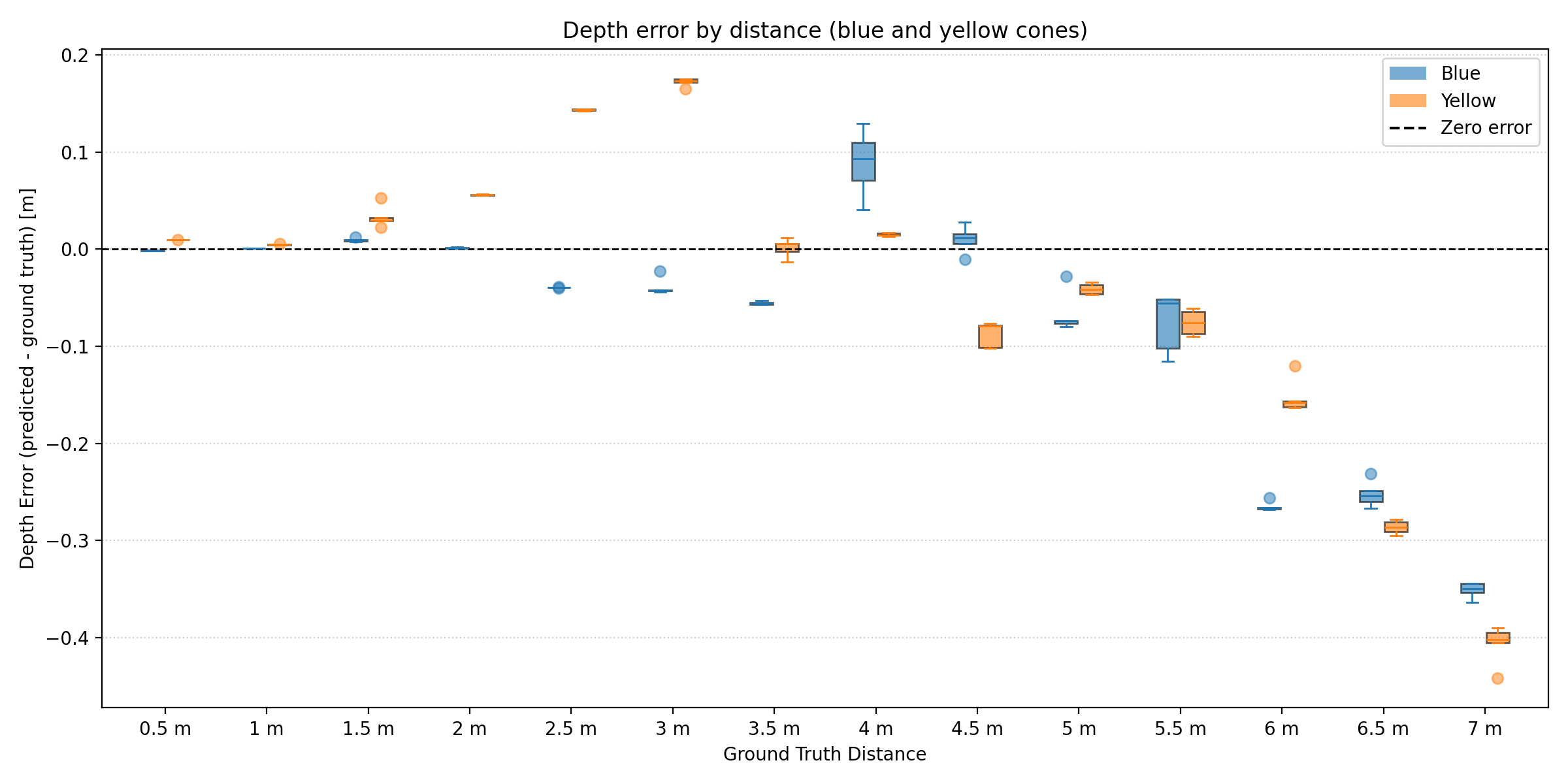
As shown in Figure 8, the depth estimation error increases approximately exponentially with distance, with a systematic bias toward underestimating range (placing objects closer than their true position). The median error reaches 0.5 m at a ground-truth distance of 7 m. A color-dependent discrepancy is also observed: blue cones are consistently estimated as closer than yellow cones, particularly at medium distances around 3 m, likely due to differences in how the neural depth model responds to each color under natural lighting. Despite this, the error margins remain acceptable for the application, as the systematic underestimation introduces a conservative bias — the vehicle initiates maneuvers earlier than strictly necessary, providing an implicit safety margin in real-world operation.
IV-C RTK data
The RTK data was evaluated comparatively with the GNSS data. This was done via a closed circuit track and measuring both the raw GNSS and the corrected coordinates via RTK. The measurements can be seen in Figures 9 and 10.


As it can be seen, the RTK provides more accurate data, and the loss of signal is more infrequent. These losses of signal in GNSS can be detected in the ”straight lines” that are shown on the graph. In the measurements done in this experiments, the precision improved up to a 12 centimeter error using RTK.
IV-D Car Controls
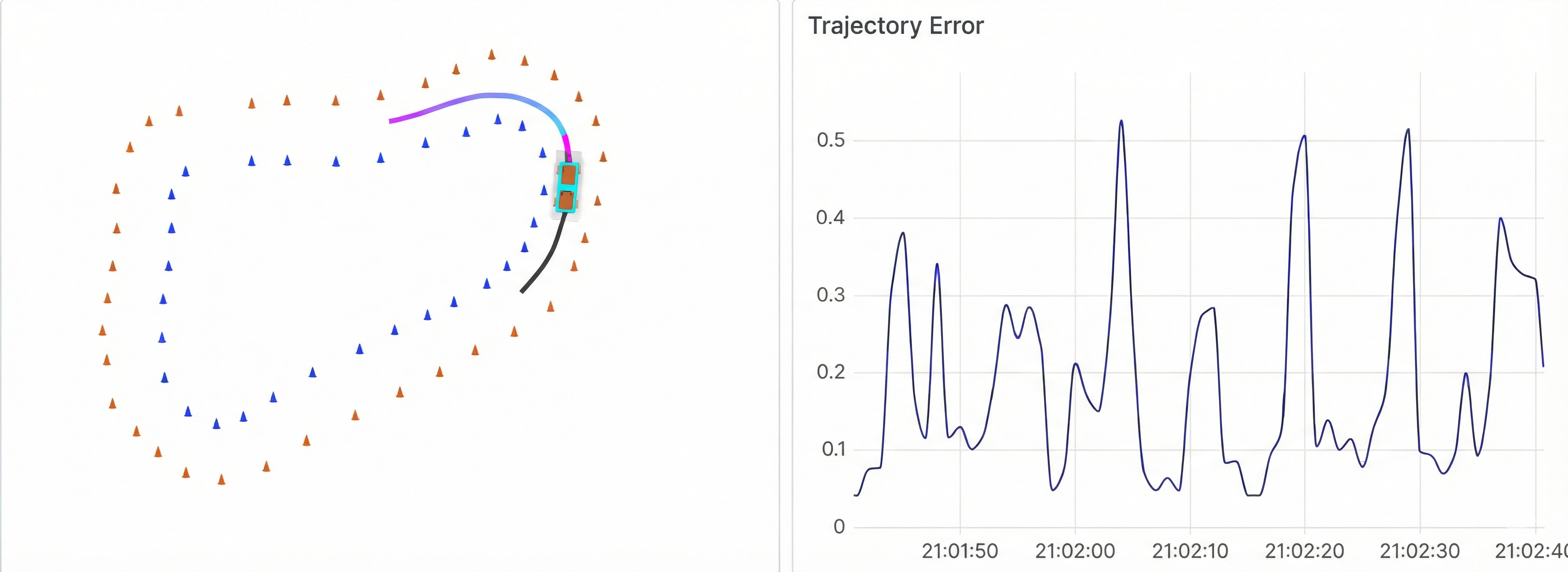
Finally, to evaluate the car control algorithms, the pipeline is deployed in a simulation environment. In this environment the track is deployed and the perception part of the pipeline is simulated, incorporating the error distribution perceived in the previous experiments. A segment of the circuit is illustrated in figure 11.
Acknowledgments
This project is supported from the Escola Superior de Enxeñería Informática and Escola Técnica Superior de Enxeñería Industrial from Universidade de Vigo. Especially with direct help from professors Dr. Javier Rodeiro Iglesias, Dr. Enrique Paz Domonte and Dr. Joaquín López Fernández.
References
- [1] “Ultralytics”. External Links: Link Cited by: §III-C2.
- [2] (2022) Experimental 2d extended kalman filter sensor fusion for low-cost gnss/imu. Measurement 200. Cited by: §III-D1.
- [3] (2023) SimpleRTK2B – budget multiband rtk gnss board data sheet. ArduSimple. Note: Based on u-blox ZED-F9P module External Links: Link Cited by: §III-A2.
- [4] (2017) High-speed tracking-by-detection without using image information. pp. 1–6. External Links: Document Cited by: §III-C3.
- [5] (2021) FS-ai ads-dv software interface specification. Institution of Mechanical Engineers. External Links: Link Cited by: §III.
- [6] (2025) Formula student uk. Institution of Mechanical Engineers. Note: Formula Student UK External Links: Link Cited by: §III.
- [7] Cited by: §II-A4.
- [8] Ultralytics yolov8 External Links: Link Cited by: §III-C2.
- [9] (2020) AMZ driverless: the full autonomous racing system. Journal of Field Robotics 37 (7), pp. 1267–1294. Cited by: §III-D1.
- [10] (1960) A new approach to linear filtering and prediction problems. Transactions of the ASME–Journal of Basic Engineering 82 (Series D), pp. 35–45. Cited by: §III-D1.
- [11] (2025) Adaptive and robust kalman filter-based fusion of imu and uwb for high-accuracy localization. IEEE Sensors Journal. Note: Demonstrates 32% accuracy improvement using EKF fusion vs raw sensors Cited by: §III-D1.
- [12] (2021) Multiple object tracking: a literature review. Artificial intelligence 293, pp. 103448. Cited by: §III-C3.
- [13] (2022) Robot operating system 2: design, architecture, and uses in the wild. Science Robotics 7 (66), pp. abm6074. External Links: Document Cited by: §III-A1.
- [14] (2023) NVIDIA jetson orin nx series: system-on-module datasheet. Note: Accessed: 2025-12-01 External Links: Link Cited by: §III-A1.
- [15] Camera calibration and 3d reconstruction. External Links: Link Cited by: §III-C4.
- [16] (2023-12) A tricycle model to accurately control an autonomous racecar with locked differential. In 2023 IEEE 11th International Conference on Systems and Control (ICSC), pp. 782–789. External Links: Link, Document Cited by: §III-D1.
- [17] (May 2022) ROS 2 Documentation. External Links: Link Cited by: §III-B.
- [18] (2018) Path planning and control in an autonomous formula student vehicle. Ph.D. Thesis, Monash University. Cited by: §III-E.
- [19] ZED 2i Camera and SDK Overview. External Links: Link Cited by: §III-C1.
- [20] (2022) ZED 2i: industrial ai stereo camera datasheet. Note: Rev. 1.0 External Links: Link Cited by: §III-A3.
- [21] (2023) A comprehensive review of yolo: from yolov1 to yolov8 and beyond. arXiv preprint arXiv:2304.00501. Cited by: §III-C2, §III-C2.
- [22] (2022) FSOCO: the formula student objects in context dataset. SAE International Journal of Connected and Automated Vehicles 5 (12-05-01-0003). Cited by: §III-C2, §IV-A.