arXiv is now an independent nonprofit! Learn more
License: CC BY 4.0
arXiv:2512.00476v2 [hep-ph] 29 Jun 2026
institutetext: a Institute for Theoretical Particle Physics, Karlsruhe Institute of Technology (KIT),
Wolfgang-Gaede-Str. 1, D-76131 Karlsruhe, Germany

QCD corrections to charged-current decays with Heavy Sterile Neutrinos in initial or final state and their impact on τ\tau decays

Tim Kretz a    Ulrich Nierste tim.kretz@kit.edu ulrich.nierste@kit.edu
Abstract

Searches for a Heavy Sterile Neutrino NN profit from precise predictions of inclusive decay rates, which enter predictions for branching fractions and lifetime. Once the decay channels into semi-hadronic final states are open, a reliable calculation of inclusive decay rates is only possible if NN is heavy enough to permit a perturbative calculation, in analogy to the well-known case of semi-hadronic τ\tau lepton decays. We adopt the popular scenario in which NN only interacts with the SM particles through NN-ν\nu_{\ell} mixing, where =e,μ,τ\ell=e,\mu,\tau. Using literature results for WW boson correlators calculated to fourth order in the strong coupling αs\alpha_{s}, we study the quality of the perturbation series for N+hadronsN\to\ell+\mbox{hadrons} to determine the mass ranges for which inclusive decay widths can be predicted in a robust way. We present novel analytic results for the decay rate of Nτ+hadronsN\to\tau+\mbox{hadrons} in terms of mτ/mNm_{\tau}/m_{N}. Our expressions equally apply to τN+hadrons\tau\to N+\mbox{hadrons}, the width of which is found to be perturbatively calculable for mN600m_{N}\lesssim 600\,MeV. Applying our result to the τ\tau lifetime, we determine the allowed parameter space for the NN-ντ\nu_{\tau} mixing angle θ\theta and mNm_{N}. We find |sinθ|0.2|\sin\theta|\leq 0.2 for mN=600m_{N}=600\,MeV and weaker bounds for a lighter NN. In the mass region mNmτm_{N}\geq m_{\tau} we find constraints from the dependence of τ\tau decay rates on cosθ\cos\theta, with |sinθ|0.12|\sin\theta|\leq 0.12 inferred from the τ\tau lifetime. Combining τπντ\tau\to\pi^{-}\nu_{\tau} and τKντ\tau\to K^{-}\nu_{\tau} data gives |sinθ|=(9.17.8+3.7)102|\sin\theta|={\left(9.1_{-7.8}^{+3.7}\right)}\cdot 10^{-2} at 1σ1\sigma while NN-ντ\nu_{\tau} mixing does not improve the agreement between theory and data for τν¯ντ\tau\to\ell\bar{\nu}_{\ell}\nu_{\tau}. We find current data for the decay rate Γ(τ+nothing)\Gamma(\tau\rightarrow\ell+\mbox{nothing}) about 1σ\sigma above the SM prediction for Γ(τν¯ντ)\Gamma(\tau\rightarrow\ell\bar{\nu}_{\ell}\nu_{\tau}), which leads to useful constraints on Γ(τXdark)\Gamma(\tau\rightarrow\ell X_{\mathrm{dark}}) or Γ(τXdarkXdark)\Gamma(\tau\rightarrow\ell X_{\mathrm{dark}}X_{\mathrm{dark}}) with dark-sector particles XdarkX_{\mathrm{dark}} and might stimulate additional experimental effort on τ+nothing\tau\rightarrow\ell+\mbox{nothing}.

preprint: P3H–25–103, TTP25-049

1 Introduction

Heavy Sterile Neutrinos (HSNs) (a.k.a. Heavy Neutral Leptons) are a widely-studied extension to the Standard Model (SM), postulated in theories of Dark Matter Asaka and Shaposhnikov (2005); Asaka et al. (2005), leptogenesis Fukugita and Yanagida (1986); Davidson and Ibarra (2002), or neutrino masses Yanagida (1979); Minkowski (1977); Gell-Mann et al. (1979); Glashow (1980); Mohapatra and Senjanovic (1980) (see Ref. Bondarenko et al. (2018) for an overview). In standard scenarios it is assumed that HSNs interact with SM particles only through mixing with the active neutrinos νe\nu_{e}, νμ\nu_{\mu}, and ντ\nu_{\tau}, so that different observables are highly correlated. In particular, WW-mediated weak decays involving an HSN NN and a charged lepton \ell in the initial or final state all involve the same element VNV_{N\ell} of the matrix describing the mixing of NN with the active neutrinos. In the most simple case one assumes that a given HSN NN only mixes with one active neutrino ν\nu_{\ell}, so that VNV_{N\ell} reduces to VN=sinθV_{N\ell}=\sin\theta with a neutrino mixing angle θ\theta. It is therefore desirable to study as many different decays as possible to first discover HSNs and subsequently corroborate or falsify the active-sterile mixing concept. In the former case one will aim at the precise determination of VNV_{N\ell} for =e,μ,τ\ell=e,\mu,\tau. In the latter case one will find apparent different values for VNV_{N\ell} in different decays and turn the attention to less minimal models featuring new interactions between NN and SM fermions, possibly mediated by new Higgs bosons or leptoquarks Robinson et al. (2019); Bernlochner et al. (2025).

The search for HSNs produced at colliders and the interpretation of experimental limits requires accurate predictions of branching fractions. In addition, it is important to know the NN lifetime to understand whether NN decays outside or within the detector. Especially interesting is the parameter space for which NN decays with a displaced decay vertex, which corresponds to an ideal, background-free signal. To predict branching fractions or lifetimes one must calculate the total decay width Γtot(N)\Gamma_{\rm tot}(N). In this paper we consider semi-hadronic decays of NN and present precise predictions for Γ(N+hadrons)\Gamma(N\to\ell+\mbox{hadrons}) for the case that the HSN mass mNm_{N} is large enough that accurate perturbative QCD predictions are possible. To this end we exploit literature results on the correlator of two charged quark currents to five-loop order of QCD Baikov et al. (2008) and add the appropriate phase-space integration to predict Γ(N+hadrons)\Gamma(N\to\ell+\mbox{hadrons}). The main purpose of this analysis is the determination of the range for mNm_{N} for which the perturbative calculation is applicable, by requiring that with higher orders in αs\alpha_{s} the size of the perturbative correction and the dependence on the unphysical renormalization scale μ\mu decrease. Specifically, if the invariant mass of the hadronic system governed by mNmm_{N}-m_{\ell} is too small, perturbation theory breaks down, and the same is true for certain larger values of mNm_{N} which are closely above the masses of the DD or BB mesons. For =e\ell=e or μ\mu we can simply use the formulae for τντ+hadrons\tau\to\nu_{\tau}+\mbox{hadrons} decays from the literature Baikov et al. (2008); Beneke and Jamin (2008), but for Γ(Nτ+hadrons)\Gamma(N\to\tau+\mbox{hadrons}) we perform a new calculation to account for mτ0m_{\tau}\neq 0 and find closed results in terms of mτ/mNm_{\tau}/m_{N} with polylogarithms (up to αs3\alpha_{s}^{3}) or a series representation (at order αs4\alpha_{s}^{4}). With this result we can further predict Γ(τN+hadrons)\Gamma(\tau\to N+\mbox{hadrons}) for the case that mNm_{N} is too large to be neglected and analyse the impact of NNντ\nu_{\tau} mixing on τ\tau lifetime and branching fractions. While our calculations are complete for Γ(τN+hadrons)\Gamma(\tau\to N+\mbox{hadrons}) and the impact of these rates on the τ\tau lifetime, the calculated N+hadronsN\to\ell+\mbox{hadrons} decay rates do not fully account for the NN lifetime, which receives further important contributions from ZZ-mediated Nν+hadronsN\to\nu_{\ell}+\mbox{hadrons} decay modes. These calculations are relegated to a future publication.

Our paper is organised as follows: In Sec. 2 we recapitulate the known results entering the calculation of the inclusive hadronic HSN decay width, in Sec. 3 we show the details of the actual calculation followed by a discussion of the phenomenology of our results in Sec. 4. We conclude in Sec. 5.

2 Preliminaries

2.1 Sterile neutrino decays at tree level

Several decays of HSN or of leptons and hadrons into HSN have been calculated at tree level Cvetič and Kim (2016); Johnson et al. (1997); Gribanov et al. (2001); Gorbunov and Shaposhnikov (2007); Atre et al. (2009); Helo et al. (2011). Here we briefly collect the tree-level results relevant to our study and introduce our notation.

An HSN NN can decay via a WW boson into a charged lepton and a quark-antiquark pair (u,d¯)(u^{\prime},\bar{d}^{\prime}). Here, we only consider cases in which NN is heavy enough to permit Nud¯N\to\ell u\bar{d} and Nus¯N\to\ell u\bar{s} decays, but for large enough values of mNm_{N} also final states with u=cu^{\prime}=c or d=bd^{\prime}=b can be accessible. The decay width reads

Γ(Nud¯)\displaystyle\Gamma(N\rightarrow\ell^{-}u^{\prime}\bar{d}^{\prime}) =NcGF2mN5|VN|2|Vud|2192π3\displaystyle=N_{c}\frac{G_{F}^{2}m_{N}^{5}|V_{N\ell}|^{2}|V_{u^{\prime}d^{\prime}}|^{2}}{192\pi^{3}}
×12(xu+xd)2(1x)2dxx(1+x2x)(xxu2xd2)λ(1,x,x2)λ(x,xu2,xd2),\displaystyle\hskip-42.67912pt\times 12\int\limits_{(x_{u^{\prime}}+x_{d^{\prime}})^{2}}^{(1-x_{\ell})^{2}}\frac{\mathrm{d}\,x}{x}(1+x_{\ell}^{2}-x)(x-x_{u^{\prime}}^{2}-x_{d^{\prime}}^{2})\sqrt{\lambda(1,x,x_{\ell}^{2})\lambda(x,x_{u^{\prime}}^{2},x_{d^{\prime}}^{2})}, (1)

here GFG_{F} is the Fermi constant, mNm_{N} is the mass of the sterile neutrino, VNV_{N\ell} parametrises the mixing between NN and ν\nu_{\ell}, VudV_{u^{\prime}d^{\prime}} is the relevant CKM matrix element, Nc=3N_{c}=3 is the number of colours, xi=mi/mNx_{i}=m_{i}/m_{N}, and λ(a,b,c)=(abc)24bc\lambda(a,b,c)=(a-b-c)^{2}-4bc is the Källén function.

Refer to caption
(a) charged current
Refer to caption
(b) neutral current
Figure 1: Tree diagrams for an HSN decay. For α=β\alpha=\beta both diagrams interfere. Diagrams were drawn with the help of TikZ-Feynman Ellis (2017).


Decay rates of an HSN into leptons Ni¯jνjN\rightarrow\ell_{i}\bar{\ell}_{j}\nu_{j} are found from Eq. (1) by setting Nc=1N_{c}=1 and Vud=1V_{u^{\prime}d^{\prime}}=1:

Γ(Nα¯βνβ)\displaystyle\Gamma(N\rightarrow\ell_{\alpha}\bar{\ell}_{\beta}\nu_{\beta})
=GF2mN5|VN|2192π3×12xβ2(1xα)2dxx(1+xα2x)(xxβ2)λ(1,x,xα2)λ(x,xβ2,0),\displaystyle=\frac{G_{F}^{2}m_{N}^{5}|V_{N\ell}|^{2}}{192\pi^{3}}\times 12\int\limits_{x_{\beta}^{2}}^{(1-x_{\alpha})^{2}}\frac{\mathrm{d}\,x}{x}(1+x_{\alpha}^{2}-x)(x-x_{\beta}^{2})\sqrt{\lambda(1,x,x_{\alpha}^{2})\lambda(x,x_{\beta}^{2},0)}, (2)

where xα=mα/mNx_{\alpha}=m_{\ell_{\alpha}}/m_{N}. This relation only holds for αβ\alpha\neq\beta. We dub the lepton directly attached to the HSN the tagging lepton (see Fig. 1). For α=β\alpha=\beta there are additional contributions to the leptonic width due to interference with the neutral current decay. The decay width becomes

Γ(\displaystyle\Gamma( Nναα¯α)=\displaystyle N\rightarrow\nu_{\alpha}\ell_{\alpha}\bar{\ell}_{\alpha})= (3)
GF2mN5|VN|2192π3×[14x2((gV22+gV)(110x2+18x436x6)\displaystyle\frac{G_{F}^{2}m_{N}^{5}|V_{N\ell}|^{2}}{192\pi^{3}}\times\bigg[\sqrt{1-4x_{\ell}^{2}}\bigg(\bigg(\frac{g_{V}^{2}}{2}+g_{V}\bigg)(1-10x_{\ell}^{2}+18x_{\ell}^{4}-36x_{\ell}^{6})
+(gA22+gA)(118x222x4+12x6)+114x22x412x6)\displaystyle\hskip 28.45274pt+\bigg(\frac{g_{A}^{2}}{2}+g_{A}\bigg)(1-18x_{\ell}^{2}-22x_{\ell}^{4}+12x_{\ell}^{6})+1-14x_{\ell}^{2}-2x_{\ell}^{4}-12x_{\ell}^{6}\bigg)
24((gV2+2gV)x6(23x2)\displaystyle\quad-24\bigg(\bigg(g_{V}^{2}+2g_{V}\bigg)x_{\ell}^{6}(2-3x_{\ell}^{2})
+(gA2+2gA)x4(22x2+x4)+x4(22x4))ln(2x1+14x2)],\displaystyle\hskip 28.45274pt+\bigg(g_{A}^{2}+2g_{A}\bigg)x_{\ell}^{4}(2-2x_{\ell}^{2}+x_{\ell}^{4})+x_{\ell}^{4}(2-2x_{\ell}^{4})\bigg)\ln\bigg(\frac{2x_{\ell}}{1+\sqrt{1-4x_{\ell}^{2}}}\bigg)\bigg],

here gA=1/2g_{A}=-1/2, gV=1/2+2sw2g_{V}=-1/2+2s_{w}^{2} with sw=sinθws_{w}=\sin\theta_{w} and the Weinberg angle θw\theta_{w}. Our results agree with those of Bodarenko et al. in Ref. Bondarenko et al. (2018). In Fig. 2 we show the decay widths as a function of mNm_{N}. The widths for ee or μ\mu as tagging leptons are almost indistinguishable.

Refer to caption
Figure 2: Decay width of an HSN into leptons. Here the notation NN\rightarrow\ell means the plotted line is the sum of all partial widths associated with the tagging lepton i.e. Γ(Ne)=Γ(Ne¯ν)\Gamma(N\rightarrow e)=\sum_{\ell}\Gamma(N\rightarrow e\bar{\ell}\nu_{\ell}). For all three channels the mixing angle is chosen as VN=103V_{N\ell}=10^{-3}.


2.2 QCD correlators

The QCD dynamics of decays of HSNs into hadrons is governed by the decays of virtual electroweak gauge bosons into hadrons. The decays of WW and ZZ bosons into hadrons have been calculated up to 𝒪(αs4)\mathcal{O}(\alpha_{s}^{4}) Baikov et al. (2012, 2008). Here we use these results to calculate the charged-current contribution to the decay of an HSN.

The optical theorem relates any inclusive decay width to the imaginary part of the self-energy of the decaying particle. The non-trivial part of the WW or ZZ boson self-energy is the correlator of two charged quark currents, namely the time ordered product of the vector and axial vector currents of the quarks jμ,ijV/A=q¯iγμ(γ5)qjj^{V/A}_{\mu,\,ij}=\bar{q}_{i}\gamma_{\mu}(\gamma_{5})q_{j}. It may be parametrized as follows Braaten et al. (1992); Chetyrkin et al. (1998)

Πμν,ijV/A(q,mi,mj,μ,αs)\displaystyle\Pi^{V/A}_{\mu\nu,\,ij}(q,m_{i},m_{j},\mu,\alpha_{s}) =idxeiqx0|T^{jμ,ijV/A(x)jν,ijV/A(0)}|0\displaystyle=i\int\mathrm{d}xe^{iqx}\braket{0|\hat{T}\{j^{V/A}_{\mu,\,ij}(x)j^{V/A\,\dagger}_{\nu,\,ij}(0)\}|0}
=gμνΠij,V/A[1](q2)+qμqνΠij,V/A[2](q2)\displaystyle=g_{\mu\nu}\Pi^{[1]}_{ij,\,V/A}(q^{2})+q_{\mu}q_{\nu}\Pi^{[2]}_{ij,\,V/A}(q^{2})
=(gμνq2+qμqν)Πij,V/A(1)(q2)+qμqνΠij,V/A(0)(q2).\displaystyle=(-g_{\mu\nu}q^{2}+q_{\mu}q_{\nu})\Pi^{(1)}_{ij,\,V/A}(q^{2})+q_{\mu}q_{\nu}\Pi^{(0)}_{ij,\,V/A}(q^{2}). (4)

Here mi,jm_{i,j} are quark masses and qq is the momentum of the gauge boson. In our case of the hadronic charged current qiq_{i} and qjq_{j} are up-type and down-type quarks, respectively. In the last line above the correlators have been decomposed into their transverse and longitudinal components

Πij,V/A(1)(q2)=Πij,V/A[1](q2)q2,Πij,V/A(0)(q2)=Πij,V/A[2](q2)+Πij,V/A[1](q2)q2.\Pi^{(1)}_{ij,\,V/A}(q^{2})=-\frac{\Pi^{[1]}_{ij,\,V/A}(q^{2})}{q^{2}},\quad\Pi^{(0)}_{ij,\,V/A}(q^{2})=\Pi^{[2]}_{ij,\,V/A}(q^{2})+\frac{\Pi^{[1]}_{ij,\,V/A}(q^{2})}{q^{2}}. (5)

In studies of τ\tau decays one commonly adopts the definition Braaten et al. (1992)

Πij,V/A(1+0)(q2)Πij,V/A(1)(q2)+Πij,V/A(0)(q2).\Pi^{(1+0)}_{ij,\,V/A}(q^{2})\equiv\Pi^{(1)}_{ij,\,V/A}(q^{2})+\Pi^{(0)}_{ij,\,V/A}(q^{2}). (6)

The correlators Π[1]\Pi^{[1]} and Π[2]\Pi^{[2]} are related to each other via a Ward identity Becchi et al. (1981); Pich (2021)

qμqνΠμν,ijV/A=q4Πij,V/A(0)=(mjmi)2ΠijS/P+(mjmi)0|q¯jqjq¯iqi|0.q^{\mu}q^{\nu}\Pi^{V/A}_{\mu\nu,\,ij}=q^{4}\Pi^{(0)}_{ij,\,V/A}=(m_{j}\mp m_{i})^{2}\Pi_{ij}^{S/P}+(m_{j}\mp m_{i})\braket{0|\bar{q}_{j}q_{j}\mp\bar{q}_{i}q_{i}|0}. (7)

This identity connects the longitudinal part of the VV or AA correlator to the scalar or pseudo-scalar correlators ΠijS/P\Pi_{ij}^{S/P}, respectively, where

ΠijS/P(q)=idxeiqx0|T^{jijS/P(x)jijS/P(0)}|0,jijS/P=q¯i(γ5)qj,\Pi^{S/P}_{ij}(q)=i\int\mathrm{d}xe^{iqx}\braket{0|\hat{T}\{j^{S/P}_{ij}(x)j^{S/P\,\dagger}_{ij}(0)\}|0},\qquad j^{S/P}_{ij}=\bar{q}_{i}(\gamma_{5})q_{j}, (8)

and the last term in Eq. (7) is the quark condensate. Thus in the chiral limit

Πij,V/A(0)=0.\Pi^{(0)}_{ij,\,V/A}=0. (9)

For the WW boson there are only contributions to the correlator by so-called non-singlet diagrams as seen in Fig. 3(a).

Refer to caption
(a) Sample non-singlet diagram to 𝒪(αS2)\mathcal{O}(\alpha_{S}^{2}).
Refer to caption
(b) One possible cut of the loop diagram in Fig. 3(a). This corresponds to the decay amplitude Wqq¯W\rightarrow q\bar{q} at 𝒪(αs2)\mathcal{O}(\alpha_{s}^{2}) interfering with the tree-level amplitude.
Figure 3: WW boson self-energy diagram contributing to the correlator.


Non-singlet diagrams only have cuts through at least two fermion lines. Cuts indicate individual contributions to the imaginary part of a loop diagram with the particles on the cut line being on-shell (see. Fig. 3(b)). From now on we adopt the chiral limit with zero quark masses. The applicability of perturbative QCD requires q2mi2q^{2}\gg m_{i}^{2}, which is certainly fulfilled for the three lightest quarks for mNa few timesΛQCDm_{N}\gtrsim\mbox{a few times}\,\Lambda_{\rm QCD}, which must be fulfilled in any perturbative QCD calculation. If one of the final state quarks is cc or bb, there is a range of q2q^{2} for which the cc or bb quark mass is non-negligible and can be included in an expansion in terms of mc,b2/q2m_{c,b}^{2}/q^{2}. These mass corrections are beyond the scope of this paper, i.e. for heavy hadrons our formulae are only valid for HSN decays with q2q^{2} large enough that mcm_{c} or mbm_{b} can be set to zero i.e. mb2>q2mc2m_{b}^{2}>q^{2}\gg m_{c}^{2} or q2mb2q^{2}\gg m_{b}^{2}.

The correlators may be expressed as a series in

aμ=αs(μ)π,a_{\mu}=\frac{\alpha_{s}(\mu)}{\pi}, (10)

where the coefficients are functions of the logarithm ln(s/μ2)\ln(-s/\mu^{2}) with s=q2s=q^{2} the invariant mass of the hadronic state and the logarithm evaluated below the branch cut according to the Feynman prescription ss+iδs\rightarrow s+i\delta, so that Imln(s/μ2iδ)=ln(s/μ2)iπ\mathrm{Im}\,\ln(-s/\mu^{2}-i\delta)=\ln(s/\mu^{2})-i\pi. Since the longitudinal part of the correlator is proportional to the square of the quark mass it will not contribute in the chiral limit (see Eq. (7)). The sum of the longitudinal and transverse part of the correlator is given by Beneke and Jamin (2008)

Πij,V/A(1+0)(s)=112π2n=0aμnk=1n+1cn,klnk(sμ2),\Pi^{(1+0)}_{ij,\,V/A}(s)=-\frac{1}{12\pi^{2}}\sum\limits_{n=0}^{\infty}a_{\mu}^{n}\sum\limits_{k=1}^{n+1}c_{n,k}\ln^{k}\bigg(\frac{-s}{\mu^{2}}\bigg), (11)

and the coefficients cn,1c_{n,1} are given by Chetyrkin et al. (1979); Dine and Sapirstein (1979); Celmaster and Gonsalves (1980); Gorishnii et al. (1988); Surguladze and Samuel (1991); Gorishnii et al. (1991); Baikov et al. (2008)

c0,1\displaystyle c_{0,1} =c1,1=1,\displaystyle=c_{1,1}=1, (12)
c2,1\displaystyle c_{2,1} =(111223ζ3)nf+3652411ζ3,\displaystyle=-\bigg(\frac{11}{12}-\frac{2}{3}\zeta_{3}\bigg)n_{f}+\frac{365}{24}-11\zeta_{3}, (13)
c3,1\displaystyle c_{3,1} =(1511621927ζ3)nf2(78472162629ζ3+259ζ5)nf\displaystyle=\bigg(\frac{151}{162}-\frac{19}{27}\zeta_{3}\bigg)n_{f}^{2}-\bigg(\frac{7847}{216}-\frac{262}{9}\zeta_{3}+\frac{25}{9}\zeta_{5}\bigg)n_{f}
+8702928811034ζ3+2756ζ5,\displaystyle\hskip 28.45274pt+\frac{87029}{288}-\frac{1103}{4}\zeta_{3}+\frac{275}{6}\zeta_{5}, (14)
c4,1\displaystyle c_{4,1} =(203324ζ3+518ζ561315832)nf3\displaystyle=\bigg(\frac{203}{324}\zeta_{3}+\frac{5}{18}\zeta_{5}-\frac{6131}{5832}\bigg)n_{f}^{3}
+(40655864ζ3+56ζ3226027ζ5+104538115552)nf2\displaystyle\hskip 28.45274pt+\bigg(-\frac{40655}{864}\zeta_{3}+\frac{5}{6}\zeta_{3}^{2}-\frac{260}{27}\zeta_{5}+\frac{1045381}{15552}\bigg)n_{f}^{2}
+(1220512ζ355ζ(3)2+29675432ζ5+66572ζ71304400710368)nf\displaystyle\hskip 28.45274pt+\bigg(\frac{12205}{12}\zeta_{3}-55\zeta(3)^{2}+\frac{29675}{432}\zeta_{5}+\frac{665}{72}\zeta_{7}-\frac{13044007}{10368}\bigg)n_{f}
731548ζ7+65945288ζ5+54458ζ325693495864ζ3+14493949920736.\displaystyle\hskip 28.45274pt-\frac{7315}{48}\zeta_{7}+\frac{65945}{288}\zeta_{5}+\frac{5445}{8}\zeta_{3}^{2}-\frac{5693495}{864}\zeta_{3}+\frac{144939499}{20736}. (15)

Here nfn_{f} denotes the number of active flavours and ζnζ(n)\zeta_{n}\equiv\zeta(n) are values of the Riemann ζ\zeta-function. To reconstruct the remaining coefficients cn,kc_{n,k} we can use the renormalization group (RG) equation. To this end, one considers the Adler function Adler (1974)

D(1+0)(s)=sddsΠij,V/A(1+0)(s),D^{(1+0)}(s)=-s\frac{d}{ds}\Pi^{(1+0)}_{ij,\,V/A}(s), (16)

which is a physical object and μ\mu-independent. Employing

μ2ddμ2Dij,V/A(1+0)(s)=0,\mu^{2}\frac{d}{d\mu^{2}}D^{(1+0)}_{ij,\,V/A}(s)=0, (17)

one finds Beneke and Jamin (2008)

c2,2\displaystyle c_{2,2} =β02c1,1\displaystyle=-\frac{\beta_{0}}{2}c_{1,1} (18)
c3,3\displaystyle c_{3,3} =β023c1,1,\displaystyle=\frac{\beta_{0}^{2}}{3}c_{1,1}, c3,2\displaystyle\qquad c_{3,2} =β12c1,1β0c2,1\displaystyle=-\frac{\beta_{1}}{2}c_{1,1}-\beta_{0}c_{2,1} (19)
c4,4\displaystyle c_{4,4} =β034c1,1,\displaystyle=-\frac{\beta_{0}^{3}}{4}c_{1,1}, c4,3\displaystyle\qquad c_{4,3} =56β1β0c1,1+β02c2,1,\displaystyle=\frac{5}{6}\beta_{1}\beta_{0}c_{1,1}+\beta_{0}^{2}c_{2,1},\quad (20)
c4,2\displaystyle\qquad c_{4,2} =12(β2c1,1+2β1c2,1+3β0c3,1),\displaystyle=-\frac{1}{2}\big(\beta_{2}c_{1,1}+2\beta_{1}c_{2,1}+3\beta_{0}c_{3,1}\big),

where cn,k=0c_{n,k}=0 if k>nk>n and n0n\neq 0 and the coefficients βi\beta_{i} of the QCD beta function are listed in Appendix A.

3 QCD Corrections to Charged Current HSN Decays

Using the correlator in Eq. (11) the differential inclusive decay rate of a HSN via a charged current reads

dΓ(NX)ds=\displaystyle\frac{d\Gamma(N\rightarrow\ell X)}{ds}= NcGF2mN5|VN|2192π3×12πmN2(1+x2smN2)λ(1,smN2,x2)\displaystyle N_{c}\frac{G_{F}^{2}m_{N}^{5}|V_{N\ell}|^{2}}{192\pi^{3}}\times\frac{12\pi}{m_{N}^{2}}\bigg(1+x_{\ell}^{2}-\frac{s}{m_{N}^{2}}\bigg)\sqrt{\lambda\bigg(1,\frac{s}{m_{N}^{2}},x_{\ell}^{2}\bigg)} (21)
×[\displaystyle\times\bigg[ (1+2smN2+x24x21+x2smN2)ImΠ(1+0)(s)2smN2ImΠ(0)(s)],\displaystyle\bigg(1+2\frac{s}{m_{N}^{2}}+x_{\ell}^{2}-\frac{4x_{\ell}^{2}}{1+x_{\ell}^{2}-\frac{s}{m_{N}^{2}}}\bigg)\mathrm{Im}\Pi^{(1+0)}(s)-2\frac{s}{m_{N}^{2}}\mathrm{Im}\Pi^{(0)}(s)\bigg],

integrating over ss, or the dimensionless variable x=s/mN2x=s/m_{N}^{2}, leads to Braaten et al. (1992)

Γ(NX)=\displaystyle\Gamma(N\rightarrow\ell X)= NcGF2mN5|VN|2192π3×12π0(1x)2𝑑x(1+x2x)λ(1,x,x2)\displaystyle N_{c}\frac{G_{F}^{2}m_{N}^{5}|V_{N\ell}|^{2}}{192\pi^{3}}\times 12\pi\int\limits_{0}^{(1-x_{\ell})^{2}}dx\,(1+x_{\ell}^{2}-x)\sqrt{\lambda(1,x,x_{\ell}^{2})} (22)
×[\displaystyle\times\bigg[ (1+2x+x24x21+x2x)ImΠ(1+0)(mN2x)2xImΠ(0)(mN2x)],\displaystyle\bigg(1+2x+x_{\ell}^{2}-\frac{4x_{\ell}^{2}}{1+x_{\ell}^{2}-x}\bigg)\mathrm{Im}\Pi^{(1+0)}(m_{N}^{2}x)-2x\mathrm{Im}\Pi^{(0)}(m_{N}^{2}x)\bigg],

with x=m/mNx_{\ell}=m_{\ell}/m_{N} and where we used

Π(J)=\displaystyle\Pi^{(J)}= |Vud|2(Πud,V(J)+Πud,A(J))+|Vus|2(Πus,V(J)+Πus,A(J))+\displaystyle|V_{ud}|^{2}\bigg(\Pi^{(J)}_{ud,\,V}+\Pi^{(J)}_{ud,\,A}\bigg)+|V_{us}|^{2}\bigg(\Pi^{(J)}_{us,\,V}+\Pi^{(J)}_{us,\,A}\bigg)+... (23)
=\displaystyle= 2(|Vud|2+|Vus|2+)ΠV(J),\displaystyle 2(|V_{ud}|^{2}+|V_{us}|^{2}+...)\Pi^{(J)}_{V},

since the vector and axial vector contribution are equal in magnitude. Here the dots indicate to the inclusion of heavier mesons i.e. DD or BB mesons. Since Π(0)mq2\Pi^{(0)}\sim m_{q}^{2} we neglect it. The integration region with small xx involves hadronic resonances while the integrand in Eq. (22) is smooth. Eq. (22) nevertheless reproduces the correct result as can be derived from analyticity properties of Π(J)\Pi^{(J)}, see Appendix B for details.

Choosing μ=mN\mu=m_{N} the imaginary part of the correlator reads

ImΠV(1+0)(mN2x)\displaystyle\mbox{Im}\,\Pi^{(1+0)}_{V}(m_{N}^{2}x) =112π2n=0amNnk=1n+1cn,kImlnk(x)\displaystyle=-\frac{1}{12\pi^{2}}\sum\limits_{n=0}^{\infty}a_{m_{N}}^{n}\sum\limits_{k=1}^{n+1}c_{n,k}\mathrm{Im}\,\ln^{k}(-x) (24)
=112π{1+amN+amN2(c2,1+2c2,2ln(x))\displaystyle=\frac{1}{12\pi}\bigg\{1+a_{m_{N}}+a_{m_{N}}^{2}(c_{2,1}+2c_{2,2}\ln(x))
+amN3(c3,1+2c3,2ln(x)(π23ln2(x))c3,3)\displaystyle\hskip 56.9055pt+a_{m_{N}}^{3}(c_{3,1}+2c_{3,2}\ln(x)-(\pi^{2}-3\ln^{2}(x))c_{3,3})
+amN4(c4,1+2c4,2ln(x)(π23ln2(x))c4,3\displaystyle\hskip 56.9055pt+a_{m_{N}}^{4}(c_{4,1}+2c_{4,2}\ln(x)-(\pi^{2}-3\ln^{2}(x))c_{4,3}
(4π2ln(x)4ln3(x))c4,4)}\displaystyle\hskip 56.9055pt-(4\pi^{2}\ln(x)-4\ln^{3}(x))c_{4,4})\bigg\}

and leads to integrals of the form

Ik=0(1x)2𝑑x((1+x2x)(1+2x+x2)4x2)λ(1,x,x2)lnk(x).I_{k}=\int\limits_{0}^{(1-x_{\ell})^{2}}dx\,\bigg((1+x_{\ell}^{2}-x)(1+2x+x_{\ell}^{2})-4x_{\ell}^{2}\bigg)\sqrt{\lambda(1,x,x_{\ell}^{2})}\ln^{k}(x). (25)

Up to k=2k=2 the integrals are analytically calculable in terms of dilogarithm and trilogarithm functions:

I0\displaystyle I_{0} =12(18x2+8x6x812x4ln(x2)),\displaystyle=\frac{1}{2}\bigg(1-8x_{\ell}^{2}+8x_{\ell}^{6}-x_{\ell}^{8}-12x_{\ell}^{4}\ln(x_{\ell}^{2})\bigg), (26)
I1\displaystyle I_{1} =1924+133x212ζ2x4133x6+1924x8\displaystyle=-\frac{19}{24}+\frac{13}{3}x_{\ell}^{2}-12\zeta_{2}x_{\ell}^{4}-\frac{13}{3}x_{\ell}^{6}+\frac{19}{24}x_{\ell}^{8}
+(3x44x6+12x8)ln(x2)\displaystyle+\bigg(-3x_{\ell}^{4}-4x_{\ell}^{6}+\frac{1}{2}x_{\ell}^{8}\bigg)\ln(x_{\ell}^{2})
+(18x2+8x6x8)ln(1x2)+12x4Li2(x2),\displaystyle+\bigg(1-8x_{\ell}^{2}+8x_{\ell}^{6}-x_{\ell}^{8}\bigg)\ln(1-x_{\ell}^{2})+12x_{\ell}^{4}\mathrm{Li}_{2}(x_{\ell}^{2}), (27)
I2\displaystyle I_{2} =26514415118x212(ζ2+2ζ3)x4+(1511816ζ2)x6+(265144+2ζ2)x8\displaystyle=\frac{265}{144}-\frac{151}{18}x_{\ell}^{2}-12(\zeta_{2}+2\zeta_{3})x_{\ell}^{4}+\bigg(\frac{151}{18}-16\zeta_{2}\bigg)x_{\ell}^{6}+\bigg(-\frac{265}{144}+2\zeta_{2}\bigg)x_{\ell}^{8}
+(196+523x248ζ2x4523x6+196x8+48x4Li2(x2))ln(1x2)\displaystyle+\bigg(-\frac{19}{6}+\frac{52}{3}x_{\ell}^{2}-48\zeta_{2}x_{\ell}^{4}-\frac{52}{3}x_{\ell}^{6}+\frac{19}{6}x_{\ell}^{8}+48x_{\ell}^{4}\mathrm{Li}_{2}(x_{\ell}^{2})\bigg)\ln(1-x_{\ell}^{2})
+(216x2+16x62x8)ln2(1x2)\displaystyle+(2-16x_{\ell}^{2}+16x_{\ell}^{6}-2x_{\ell}^{8})\ln^{2}(1-x_{\ell}^{2})
+(x2+152x4+233x61912x8\displaystyle+\bigg(-x_{\ell}^{2}+\frac{15}{2}x_{\ell}^{4}+\frac{23}{3}x_{\ell}^{6}-\frac{19}{12}x_{\ell}^{8}
+(1+8x28x6+x8)ln(1x2)+24x4ln2(1x2)12x4Li2(x2))ln(x2)\displaystyle+(-1+8x_{\ell}^{2}-8x_{\ell}^{6}+x_{\ell}^{8})\ln(1-x_{\ell}^{2})+24x_{\ell}^{4}\ln^{2}(1-x_{\ell}^{2})-12x_{\ell}^{4}\mathrm{Li}_{2}(x_{\ell}^{2})\bigg)\ln(x_{\ell}^{2})
+(1+8x2+12x4+8x6x8)Li2(x2)\displaystyle+(-1+8x_{\ell}^{2}+12x_{\ell}^{4}+8x_{\ell}^{6}-x_{\ell}^{8})\mathrm{Li}_{2}(x_{\ell}^{2})
+24x4Li3(x2)+48x4Li3(1x2).\displaystyle+24x_{\ell}^{4}\mathrm{Li}_{3}(x_{\ell}^{2})+48x_{\ell}^{4}\mathrm{Li}_{3}(1-x_{\ell}^{2}). (28)

In Appendix C we give approximations to these integrals for easier use.

We next derive a new analytical result holding as well for k3k\geq 3, defined in terms of a well converging sum. To do this we first use the following series representation of the square root of the Källén function,

dndxnλ(1,x,x2)=\displaystyle\frac{\mathrm{d}^{n}}{\mathrm{d}x^{n}}\sqrt{\lambda(1,x,x_{\ell}^{2})}= j=0n2(1)nj(12)nj(2j1)!!(n2j)\displaystyle\sum\limits_{j=0}^{\lfloor\frac{n}{2}\rfloor}(-1)^{n-j}\bigg(-\frac{1}{2}\bigg)_{n-j}(2j-1)!!\begin{pmatrix}n\\ 2j\end{pmatrix} (29)
×(λ(1,x,x2))n2j(λ′′(1,x,x2))j(λ(1,x,x2))2(nj)12,\displaystyle\hskip 28.45274pt\times\frac{\bigg(\lambda^{\prime}(1,x,x_{\ell}^{2})\bigg)^{n-2j}\bigg(\lambda^{\prime\prime}(1,x,x_{\ell}^{2})\bigg)^{j}}{\bigg(\lambda(1,x,x_{\ell}^{2})\bigg)^{\frac{2(n-j)-1}{2}}},

where (a)n=a(a+1)(a+2)(a+n1)(a)_{n}=a(a+1)(a+2)\cdot...\cdot(a+n-1) is the Pochhammer symbol, j\lfloor j\rfloor is the floor function (rounding a real number to the nearest smaller integer number) and

λ(1,x,x2)\displaystyle\lambda(1,x,x_{\ell}^{2}) =x22x(1+x2)+(1x2)2,\displaystyle={{x^{2}-2x(1+x_{\ell}^{2})+(1-x_{\ell}^{2})^{2}}}, (30)
λ(1,x,x2)\displaystyle\lambda^{\prime}(1,x,x_{\ell}^{2}) =dλ(1,x,x2)dx=2x2(1+x2),\displaystyle=\frac{\mathrm{d}\lambda(1,x,x_{\ell}^{2})}{\mathrm{d}x}={{2x-2(1+x_{\ell}^{2})}}, (31)
λ′′(1,x,x2)\displaystyle\lambda^{\prime\prime}(1,x,x_{\ell}^{2}) =d2λ(1,x,x2)dx2=2.\displaystyle=\frac{\mathrm{d}^{2}\lambda(1,x,x_{\ell}^{2})}{\mathrm{d}x^{2}}=2. (32)

We write

Ik(x2,a)=n=01n!An(x2)Bn,k(x2,a)I_{k}(x_{\ell}^{2},a)=\sum\limits_{n=0}^{\infty}\frac{1}{n!}A_{n}(x_{\ell}^{2})B_{n,k}(x_{\ell}^{2},a) (33)

with

An(x2)\displaystyle A_{n}(x_{\ell}^{2}) dndxnλ(1,x,x2)|x=0\displaystyle\equiv\,\left.\frac{\mathrm{d}^{n}}{\mathrm{d}x^{n}}\sqrt{\lambda(1,x,x_{\ell}^{2})}\right|_{x=0}
=j=0n2(1)j(12)nj(2j1)!!(n2j)2nj(1+x2)n2j(1x2)12(nj),\displaystyle\hskip-21.33955pt={{\sum\limits_{j=0}^{\lfloor\frac{n}{2}\rfloor}(-1)^{j}\bigg(-\frac{1}{2}\bigg)_{n-j}(2j-1)!!\begin{pmatrix}n\\ 2j\end{pmatrix}2^{n-j}(1+x_{\ell}^{2})^{n-2j}(1-x_{\ell}^{2})^{1-2(n-j)},}} (34)

and

Bn,k(x2,a)\displaystyle B_{n,k}(x_{\ell}^{2},a) 0a𝑑x((1+x2x)(1+2x+x2)4x2)xnlnk(x)\displaystyle\equiv\,\int\limits_{0}^{a}\!dx\,\bigg((1+x_{\ell}^{2}-x)(1+2x+x_{\ell}^{2})-4x_{\ell}^{2}\bigg)x^{n}\ln^{k}(x)
=2In+2,k(a)+(1+x2)In+1,k(a)+(1x2)2In,k(a).\displaystyle=\,-2I_{n+2,k}\left(a\right)+(1+x_{\ell}^{2})I_{n+1,k}\left(a\right)+(1-x_{\ell}^{2})^{2}I_{n,k}\left(a\right). (35)

The integrals in this expression are given by

In,k(a)\displaystyle I_{n,k}(a) 0a𝑑xxnlnkx\displaystyle\equiv\,\int_{0}^{a}dx\,x^{n}\ln^{k}x
=an+1l=0k(k)l(n+1)l1lnkla,\displaystyle=\,a^{n+1}\sum_{l=0}^{k}(-k)_{l}(n+1)^{-l-1}\ln^{k-l}a, (36)

which completes the calculation of IkI_{k} in Eq. (25).

Inserting Eq. (24) into Eq. (22) and using Eq. (25) finally gives the full semi-hadronic width for decays of sterile neutrinos lighter than the D+D^{+} meson

Γ(NX)=\displaystyle\Gamma(N\rightarrow\ell X)= NcGF2mN5|VN|2192π32(|Vud|2+|Vus|2)\displaystyle N_{c}\frac{G_{F}^{2}m_{N}^{5}|V_{N\ell}|^{2}}{192\pi^{3}}\cdot 2(|V_{ud}|^{2}+|V_{us}|^{2}) (37)
×[I0(x2,(1x)2)c0,1+amNc1,1I0(x2,(1x)2)\displaystyle\hskip-56.9055pt\times\bigg[I_{0}(x_{\ell}^{2},(1-x_{\ell})^{2})c_{0,1}+a_{m_{N}}c_{1,1}I_{0}(x_{\ell}^{2},(1-x_{\ell})^{2})
+amN2[c2,1I0(x2,(1x)2)+2c2,2I1(x2,(1x)2)]\displaystyle\hskip-56.9055pt+a_{m_{N}}^{2}\big[c_{2,1}I_{0}(x_{\ell}^{2},(1-x_{\ell})^{2})+2c_{2,2}I_{1}(x_{\ell}^{2},(1-x_{\ell})^{2})\big]
+amN3[c3,1I0(x2,(1x)2)+2c3,2I1(x2,(1x)2)\displaystyle\hskip-56.9055pt+a_{m_{N}}^{3}\big[c_{3,1}I_{0}(x_{\ell}^{2},(1-x_{\ell})^{2})+2c_{3,2}I_{1}(x_{\ell}^{2},(1-x_{\ell})^{2})
(π2I0(x2,(1x)2)3I2(x2,(1x)2))c3,3]\displaystyle-(\pi^{2}I_{0}(x_{\ell}^{2},(1-x_{\ell})^{2})-3I_{2}(x_{\ell}^{2},(1-x_{\ell})^{2}))c_{3,3}\big]
+amN4[c4,1I0(x2,(1x)2)+2c4,2I1(x2,(1x)2)\displaystyle\hskip-56.9055pt+a_{m_{N}}^{4}\big[c_{4,1}I_{0}(x_{\ell}^{2},(1-x_{\ell})^{2})+2c_{4,2}I_{1}(x_{\ell}^{2},(1-x_{\ell})^{2})
(π2I0(x2,(1x)2)3I2(x2,(1x)2))c4,3\displaystyle-(\pi^{2}I_{0}(x_{\ell}^{2},(1-x_{\ell})^{2})-3I_{2}(x_{\ell}^{2},(1-x_{\ell})^{2}))c_{4,3}
(4π2I1(x2,(1x)2)4I3(x2,(1x)2))c4,4]].\displaystyle-(4\pi^{2}I_{1}(x_{\ell}^{2},(1-x_{\ell})^{2})-4I_{3}(x_{\ell}^{2},(1-x_{\ell})^{2}))c_{4,4}\big]\bigg].

Logarithms involving the renormalization scale may be reconstructed by using the relation in Appendix A. Sterile neutrinos heavier than the D+D^{+} meson also obey the relation above once the corresponding CKM element as well as threshold effects are included.

Additionally we also calculated the integral in Eq. (25) for an arbitrary upper limit of the hadronic invariant mass, to permit the calculation of the integrated spectrum of the decay

Γcut(NX)\displaystyle\Gamma_{\mathrm{cut}}(N\rightarrow\ell X) =0smax𝑑sdΓ(NX)ds,smax[𝒪(1 GeV),(mNm)2],\displaystyle=\int\limits_{0}^{s_{\mathrm{max}}}ds\,\frac{d\Gamma(N\rightarrow\ell X)}{ds},\quad s_{\mathrm{max}}\in[\mathcal{O}($1\text{\,}\mathrm{GeV}$),(m_{N}-m_{\ell})^{2}],
=0xmax𝑑xdΓ(NX)dx\displaystyle=\int\limits_{0}^{x_{\mathrm{max}}}dx\,\frac{d\Gamma(N\rightarrow\ell X)}{dx} (38)

where we defined xmax=smax/mN2x_{\mathrm{max}}=s_{\mathrm{max}}/m_{N}^{2}. Γcut(NX)\Gamma_{\mathrm{cut}}(N\rightarrow\ell X) obeys Eq. (37) with Ik=Ik(x2,xmax)I_{k}=I_{k}(x_{\ell}^{2},x_{\mathrm{max}}). Up to k=2k=2 we found a closed analytical form of the Ik(x2,xmax)I_{k}(x_{\ell}^{2},x_{\mathrm{max}}). The expressions are found in Appendix D, but the calculation from Eq. (33) is easier even for k2k\leq 2.

4 Numerical Analysis

4.1 Quality of the perturbation series

Perturbative QCD describes observables in an expansion of the strong coupling constant accurately if the relevant energy scale μ\mu is large enough such that αs\alpha_{s} is small. Any observable OμO_{\mu} at the scale μ\mu may be written as

Oμ=nrnαs(μ)n=r0+r1αs(μ)+r2αs(μ)2+𝒪(αs(μ)3).O_{\mu}=\sum\limits_{n}r_{n}\alpha_{s}(\mu)^{n}=r_{0}+r_{1}\alpha_{s}(\mu)+r_{2}\alpha_{s}(\mu)^{2}+\mathcal{O}(\alpha_{s}(\mu)^{3}). (39)

However, at small scales (μ𝒪(1 GeV)\mu\sim\mathcal{O}($1\text{\,}\mathrm{GeV}$)) the strong coupling constant becomes large and an expansion in αs\alpha_{s} is no longer guaranteed to converge. For the τ\tau lepton with a mass of mτ=1.776 GeVm_{\tau}=$1.776\text{\,}\mathrm{GeV}$ it was only possible to correctly describe the inclusive hadronic decay width through the inclusion of five-loop corrections. Only at the five-loop level does the perturbative description become stable i.e. the 𝒪(αs4)\mathcal{O}(\alpha_{s}^{4}) corrections lead to a significantly reduced dependence on the renormalization scale Baikov et al. (2008). In the case of a HSN with mass comparable to the τ\tau the kinematics is, up to the mass of the lepton attached to the HSN, the same. Setting m=0m_{\ell}=0 leads to the same numerical coefficients as in τ\tau decay

Γ(NX)|Vud|2+|Vus|2=\displaystyle\frac{\Gamma(N\rightarrow\ell X)}{|V_{ud}|^{2}+|V_{us}|^{2}}= NcGF2mN5|VN|2192π3\displaystyle N_{c}\frac{G_{F}^{2}m_{N}^{5}|V_{N\ell}|^{2}}{192\pi^{3}} (40)
×[1+amN+5.202amN2+26.366amN3+127.079amN4],\displaystyle\times\bigg[1+a_{m_{N}}+5.202a_{m_{N}}^{2}+26.366a_{m_{N}}^{3}+127.079a_{m_{N}}^{4}\bigg],

perfectly agreeing with Ref. Baikov et al. (2008). For a HSN mass around 3 GeV3\text{\,}\mathrm{GeV} the inclusive semi-hadronic decay with =τ\ell=\tau in the final state is kinematically accessible. The lepton mass ratio is then sizable, xτ=0.592x_{\tau}=0.592, and

Γ(NτX)|Vud|2+|Vus|2=\displaystyle\frac{\Gamma(N\rightarrow\tau X)}{|V_{ud}|^{2}+|V_{us}|^{2}}= NcGF2mN5|VN|2192π3\displaystyle N_{c}\frac{G_{F}^{2}m_{N}^{5}|V_{N\ell}|^{2}}{192\pi^{3}} (41)
×0.071[1+amN+8.376amN2+74.605amN3+669.805amN4],\displaystyle\times 0.071\bigg[1+a_{m_{N}}+8.376a_{m_{N}}^{2}+74.605a_{m_{N}}^{3}+669.805a_{m_{N}}^{4}\bigg],

largely reducing the decay rate and making the convergence of the perturbative series worse.

In Fig. 4 we show the full decay width. The widths for =e\ell=e and =μ\ell=\mu are indistinguishable. For mNmμ+mDm_{N}\geq m_{\mu}+m_{D} the decay channel into charmed mesons opens up. For this reason we omit the region mN[mμ+mD,3 GeV]m_{N}\in[m_{\mu}+m_{D},$3\text{\,}\mathrm{GeV}$] in Fig. 4 as here there are resonances of charmed mesons. They are dominated by non-perturbative effects making an accurate perturbative description in this region impossible. We show the =μ\ell=\mu rate again beyond mN3 GeVm_{N}\geq$3\text{\,}\mathrm{GeV}$. We have computed the error band by taking as uncertainty the difference between the minimal and maximal width with respect to the renormalization scale i.e. σΓ=(maxΓN(μ)minΓN(μ))/2\sigma_{\Gamma}=(\max\,\Gamma_{N}(\mu)-\min\,\Gamma_{N}(\mu))/2 for 0.8 GeVμ3.5 GeV$0.8\text{\,}\mathrm{GeV}$\leq\mu\leq$3.5\text{\,}\mathrm{GeV}$. Since we did not include charm mass corrections we expect an additional error of 𝒪(mD2/q2)=𝒪(40%)\mathcal{O}(m_{D}^{2}/q^{2})=\mathcal{O}(40\%) for mN=3 GeVm_{N}=$3\text{\,}\mathrm{GeV}$, which is not shown.

Refer to caption
Figure 4: Hadronic decay widths Γ(NX)\Gamma(N\rightarrow\ell X) for the tagging leptons =μ,τ\ell=\mu,\tau with a mixing angle of VN=103V_{N\ell}=10^{-3}. The width for =e\ell=e looks like the =μ\ell=\mu width. The numerics of the running coupling were calculated with the help of RunDec Chetyrkin et al. (2000); Herren and Steinhauser (2018). We do not show the region mN[mμ+mD,3 GeV]m_{N}\in[m_{\mu}+m_{D},$3\text{\,}\mathrm{GeV}$] where we expect large non-perturbative effects. The error band is taken as the difference between minimum and maximum of the width with respect to the renormalization scale σΓ=(maxΓN(μ)minΓN(μ))/2\sigma_{\Gamma}=(\max\,\Gamma_{N}(\mu)-\min\,\Gamma_{N}(\mu))/2 for 0.8 GeVμ3.5 GeV$0.8\text{\,}\mathrm{GeV}$\leq\mu\leq$3.5\text{\,}\mathrm{GeV}$. We do not include the uncertainty from our omission of quark masses, which can be sizable, 𝒪(mD2/q2)=𝒪(40%)\mathcal{O}(m_{D}^{2}/q^{2})=\mathcal{O}(40\%) for mN=3 GeVm_{N}=$3\text{\,}\mathrm{GeV}$, beyond the charm production threshold.


In Fig. 5 we plot the effect of each order in αs\alpha_{s} on the total decay width for =μ\ell=\mu. For small HSN masses, close to the kinematic threshold of multi-hadron production, we see that including more corrections in αs\alpha_{s} does not improve the convergence. This is even more pronounced in Fig. 5(b) where the relative increase compared to the leading order is large for HSN masses in a window below 1 GeV\sim$1\text{\,}\mathrm{GeV}$. Beyond 1 GeV1\text{\,}\mathrm{GeV} the perturbative behavior rapidly improves and higher order corrections become smaller with higher orders in αs\alpha_{s} in relation to the leading order.

Refer to caption
(a) Inclusive HSN decay width with =μ\ell=\mu. Here VN=μ=103V_{N\ell=\mu}=10^{-3}.
Refer to caption
(b) ΓN\Gamma_{N} at different orders of αs\alpha_{s}, normalized to the LO result.
Figure 5: Inclusive decay width ΓN=Γ(NμX)\Gamma_{N}=\Gamma(N\rightarrow\mu X) as a function of mNm_{N}.


We specifically analyzed the scale dependence of the widths by expressing amNa_{m_{N}} in terms of logarithms of the renormalization scale μ\mu and the HSN mass as seen in Appendix A.

Refer to caption
Refer to caption
Refer to caption
Refer to caption
Figure 6: Scale dependence of the inclusive decay width ΓN=Γ(NμX)\Gamma_{N}=\Gamma(N\rightarrow\mu X) for different HSN masses.


In Fig. 6 the scale dependence for different HSN masses is shown. The scale dependence is very strong close to the kinematic threshold. Increasing the mass of the HSN the scale dependence reduces. We see that HSN masses around 1.5 GeV1.5\text{\,}\mathrm{GeV}, including the highest order corrections in αs\alpha_{s} available, lead to a flat scale dependence.

In the =τ\ell=\tau final state lepton case the discussion is qualitatively similar to the =e\ell=e and =μ\ell=\mu case. Looking only at the decay width in Fig. 7(a) the effect of poor convergence does not seem to be as pronounced, however, in absolute values it is comparable to the decay into a muon as seen in Fig. 7(b). As in the muon case, the quality of the perturbative series rapidly increases for larger HSN masses.

Refer to caption
(a) Inclusive HSN decay width with =τ\ell=\tau. Here VN=τ=103V_{N\ell=\tau}=10^{-3}.
Refer to caption
(b) ΓN\Gamma_{N} at different orders of αs\alpha_{s}, normalized to the LO result.
Figure 7: Inclusive decay width ΓN=Γ(NτX)\Gamma_{N}=\Gamma(N\rightarrow\tau X)


In Fig. 8 the scale dependence for different HSN masses is shown. The scale dependence reduces for larger masses. At a HSN mass of 3 GeV3\text{\,}\mathrm{GeV} the 𝒪(αs4)\mathcal{O}(\alpha_{s}^{4}) corrections reduce the scale dependence significantly.

Refer to caption
Refer to caption
Refer to caption
Refer to caption
Figure 8: Scale dependence of the inclusive decay width ΓN=Γ(NτX)\Gamma_{N}=\Gamma(N\rightarrow\tau X) for different HSN masses.


For larger HSN masses already lower order results show a satisfactory small scale dependence.

4.2 Branching ratios of HSN

Without the neutral current contributions mediated by the ZZ boson one cannot calculate the total width, which is needed for branching ratio predictions. However ratios of branching ratios for the charged decays can be calculated

κP=Br(NP)Br(NX)=Γ(NP)Γ(NX),\kappa_{\ell}^{P}=\frac{Br(N\rightarrow\ell P)}{Br(N\rightarrow\ell X)}=\frac{\Gamma(N\rightarrow\ell P)}{\Gamma(N\rightarrow\ell X)}, (42)

here P=π+,K+,D+,P=\pi^{+},K^{+},D^{+},... is some meson, Γ(NP)\Gamma(N\rightarrow\ell P) is the width of a HSN into a meson

Γ(NP)=GF2mN3|VN|216π|Vud|2fP2[(1x2)2xP2(1+x2)]λ(1,x2,xP2),\Gamma(N\rightarrow\ell P)=\frac{G_{F}^{2}m_{N}^{3}|V_{N\ell}|^{2}}{16\pi}|V_{u^{\prime}d^{\prime}}|^{2}f_{P}^{2}\bigg[(1-x_{\ell}^{2})^{2}-x_{P}^{2}(1+x_{\ell}^{2})\bigg]\sqrt{\lambda(1,x_{\ell}^{2},x_{P}^{2})}, (43)

where fPf_{P} is the meson decay constant, |Vud||V_{u^{\prime}d^{\prime}}| is the relevant CKM matrix element, and xi=mi/mNx_{i}=m_{i}/m_{N}, and Γ(NX)\Gamma(N\rightarrow\ell X) is the fully inclusive semi-hadronic decay rate as given in Eq. (37). For our predictions of κP\kappa_{\ell}^{P} we assume mN>1.5 GeVm_{N}>$1.5\text{\,}\mathrm{GeV}$ for electron and muon tagging and mN>3 GeVm_{N}>$3\text{\,}\mathrm{GeV}$ for tau tagging.

Refer to caption
(a) κμP\kappa_{\mu}^{P}
Refer to caption
(b) κτP\kappa_{\tau}^{P}
Figure 9: NPN\rightarrow\ell P branching fractions (normalized to Br(NN)Br(N\rightarrow\ell N)) for P=π+,K+,Ds+P=\pi^{+},K^{+},D_{s}^{+}, see Eq. (42). We use fD=212.0±0.7 MeVf_{D}=$212.0\pm 0.7\text{\,}\mathrm{MeV}$, fDs=249.9±0.5 MeVf_{D_{s}}=$249.9\pm 0.5\text{\,}\mathrm{MeV}$ Bazavov and others (2018); Carrasco and others (2015); Aoki and others (2024), and |Vcd|=0.221±0.004|V_{cd}|=0.221\pm 0.004, and |Vcs|=0.975±0.006|V_{cs}|=0.975\pm 0.006 Navas and others (2024). The error bands are the same as in Fig. 4.


In Fig. 9 the κ\kappa-ratio for muon and tau tagging are shown. In both cases pions dominate the decay and only a few CKM-suppressed decays to kaons are predicted. For this reason we omit decays to DD mesons as they are more suppressed than those into kaons due to the smaller phase space. In addition we also show the impact of the inclusion of DsD_{s} mesons. DsD_{s} mesons are produced copiously beyond the charm threshold as Vcs1V_{cs}\approx 1. We exclude the region mN[mμ+mD,3 GeV]m_{N}\in[m_{\mu}+m_{D},$3\text{\,}\mathrm{GeV}$] as here non-perturbative charm resonance effects dominate the width. As long as the decay channels to charmed final states are absent, at least 12%12\% of the charged-current decays of HSN are NπN\rightarrow\ell\pi for all considered values of mNm_{N}.

4.3 Constraints on θNτ\theta_{N\tau} from the τ\tau lifetime

The current world average of the τ\tau-lifetime

ττexp.=290.29±0.53 fsBanerjee and others (2024)\tau_{\tau}^{\mathrm{exp.}}=$290.29\pm 0.53\text{\,}\mathrm{fs}$\quad\text{\cite[cite]{\@@bibref{Authors Phrase1YearPhrase2}{HeavyFlavorAveragingGroupHFLAV:2024ctg}{\@@citephrase{(}}{\@@citephrase{)}}}} (44)

agrees with the SM theory prediction

ττSM=288.59±2.31 fsNavas and others (2024); Erler and Luo (2003).\tau_{\tau}^{\mathrm{SM}}=$288.59\pm 2.31\text{\,}\mathrm{fs}$\quad\text{\cite[cite]{\@@bibref{Authors Phrase1YearPhrase2}{ParticleDataGroup:2024cfk,Erler:2002bu}{\@@citephrase{(}}{\@@citephrase{)}}}.} (45)

Whenever a sterile neutrino interaction is present it comes with a factor of the mixing angle VNτ=sinθNτV_{N\tau}=\sin\theta_{N\tau}. At the same time SM neutrino interactions receive a contribution involving cosθNτ\cos\theta_{N\tau}. Mixing is possible between one or more generations of SM neutrinos. If there is mixing with νe\nu_{e} or νμ\nu_{\mu} this has an impact on the Fermi constant. A complete analysis including also mixing with ee or μ\mu requires a full electroweak fit (see Ref.Lacker and Menzel (2010)) and is beyond the scope of this work. Hence we only look at mixing with ντ\nu_{\tau}, and define θθNτ\theta\equiv\theta_{N\tau}. Then a sterile neutrino will modify the total width, implying the following constraint on θ\theta:

ττexp.=1τscos2θ(1τs)ΓSM+sin2θΓN,\tau_{\tau}^{\mathrm{exp.}}=\frac{1-\mathcal{B}^{s}_{\tau}}{\cos^{2}\theta\,(1-\mathcal{B}^{s}_{\tau})\Gamma^{\mathrm{SM}}+\sin^{2}\theta\,\Gamma^{N}}, (46)

where τs=0.0292\mathcal{B}^{s}_{\tau}=0.0292 Navas and others (2024) is the branching fraction of τ\tau decays into strange final states, (1τs)ΓSM(1-\mathcal{B}^{s}_{\tau})\Gamma^{\mathrm{SM}} is the SM width involving leptonic and non-strange hadronic decays, and ΓN\Gamma^{N} is the non-strange sterile neutrino contribution, i.e. the τNX\tau\rightarrow NX decay rate with XX being a non-strange hadronic final state. (1τs)/ττexp.(1-\mathcal{B}^{s}_{\tau})/\tau_{\tau}^{\mathrm{exp.}} is the experimentally determined total decay rate into non-strange particles; our approach follows Ref. Navas and others (2024). ΓSM\Gamma^{\mathrm{SM}} is calculated as ΓSM=1/ττSM\Gamma^{\mathrm{SM}}=1/\tau_{\tau}^{\mathrm{SM}} and ΓN\Gamma^{N} follows from Eq. (37) by replacing VN1V_{N\ell}\rightarrow 1, Vus0V_{us}\rightarrow 0, mNmτm_{N}\rightarrow m_{\tau}, and Ik(x2,(1x)2)Ik(mN2/mτ2,(1mN/mτ)2)I_{k}(x_{\ell}^{2},(1-x_{\ell})^{2})\rightarrow I_{k}(m_{N}^{2}/m_{\tau}^{2},(1-m_{N}/m_{\tau})^{2}). For the strong coupling constant we use αsnf=3(mτ)=0.316\alpha_{s}^{n_{f}=3}(m_{\tau})=0.316 which we obtain by using the weighted average αsnf=5(MZ)=0.1182\alpha_{s}^{n_{f}=5}(M_{Z})=0.1182 of all measurements listed in the PDG Navas and others (2024), except the one using τ\tau decay, and running αs(MZ)\alpha_{s}(M_{Z}) down to mτm_{\tau}.

Refer to caption
Refer to caption
Refer to caption
Refer to caption
Figure 10: Scale dependence of the inclusive τ\tau decay width with a final state HSN for different HSN masses mNm_{N}.


In Fig. 10 we show the renormalization scale dependence of the τ\tau decay width. At 𝒪(αs4)\mathcal{O}(\alpha_{s}^{4}) the scale dependence remains sufficiently flat up to HSN masses around mN=600 MeVm_{N}=$600\text{\,}\mathrm{MeV}$. For larger HSN masses the perturbative description becomes poorer.

Sterile neutrinos solely produced through mixing with ντ\nu_{\tau} will always decrease the τ\tau width and thus prolong the predicted lifetime, possibly bringing it into tension with the experimental value. This is so, because the decay rate to ντ\nu_{\tau} is decreased by a factor of cos2θNτ\cos^{2}\theta_{N\tau} while the additional decay channel with NN, proportional to sin2θNτ\sin^{2}\theta_{N\tau} involves phase-space suppression. Neglecting electroweak corrections in ΓN\Gamma^{N} we use Eq. (46) to determine the parameter space for θ\theta and mNm_{N} in agreement with the measured τ\tau lifetime, see Fig. 11, which shows the 1σ1\sigma region of the allowed mixing angle and HSN mass, up to mN600 MeVm_{N}\leq$600\text{\,}\mathrm{MeV}$. We further show the allowed region when the experimental value in Eq. (44) is varied in the 3σ\sigma range, while we do not triple the theoretical uncertainty. For mN>600 MeVm_{N}>$600\text{\,}\mathrm{MeV}$ we continue our 1σ1\sigma and 3σ3\sigma lines for illustration, bearing in mind that the quality of the perturbative calculation diminishes significantly for mN600 MeVm_{N}\gtrsim$600\text{\,}\mathrm{MeV}$, while the perturbation series for the inclusive hadronic τ\tau decay width converges well for mN600 MeVm_{N}\lesssim$600\text{\,}\mathrm{MeV}$.

Refer to caption
Figure 11: Allowed parameter space deduced from the measured τ\tau lifetime in Eq. (44) via Eq. (46) at the 1σ1\sigma (purple) and 3σ3\sigma (purple and blue) levels. For mN600 MeVm_{N}\leq$600\text{\,}\mathrm{MeV}$ we trust the perturbative calculation. The dashed lines for mN>600 MeVm_{N}>$600\text{\,}\mathrm{MeV}$ indicate the perturbative result in a region where the description is no longer reliable.


Eq. (46) holds for any value of mNm_{N}, in particular, it also holds for mN>mτm_{N}>m_{\tau}. In this case ΓN=0\Gamma_{N}=0 and Eq. (46) becomes

sin2θ=1ττth.ττexp.=0.00586±0.00816,\sin^{2}\theta=1-\frac{\tau_{\tau}^{\mathrm{th.}}}{\tau_{\tau}^{\mathrm{exp.}}}=0.00586\pm 0.00816, (47)

which leads to

|sinθ|11.8102at  1σ.|\sin\theta|{\leq 11.8}\cdot 10^{-2}\quad\mathrm{at}\,\,1\sigma. (48)

4.4 Contributions on θNτ\theta_{N\tau} for mN>mτm_{N}>m_{\tau} from τ\tau branching fractions

HSNs heavier than τ\tau affect ττ\tau_{\tau} in Eq. (46) indirectly through the cosine of the mixing angle. To study this scenario we look at the decays τπντ\tau^{-}\rightarrow\pi^{-}\nu_{\tau}, τKντ\tau^{-}\rightarrow K^{-}\nu_{\tau}, and τντν¯\tau\rightarrow\nu_{\tau}\ell\bar{\nu}_{\ell} Helo et al. (2011); Kobach and Dobbs (2015). This will allow us to bypass the theoretical uncertainty of the total hadronic width feeding into ττ\tau_{\tau} in Eq. (45). The decay widths of interest read

Γ(τPντ)=\displaystyle\Gamma(\tau\rightarrow P\nu_{\tau})= cos2θΓSM(τPντ)\displaystyle\cos^{2}\theta\Gamma_{\mathrm{SM}}(\tau\rightarrow P\nu_{\tau}) (49)
=\displaystyle= GF2mτ3cos2θ16π|Vuq|2fP2(1mP2mτ2)2(1+δRC(P)),\displaystyle\frac{G_{F}^{2}m_{\tau}^{3}\cos^{2}\theta}{16\pi}|V_{uq}|^{2}f_{P}^{2}\bigg(1-\frac{m_{P}^{2}}{m_{\tau}^{2}}\bigg)^{2}\big(1+\delta_{\mathrm{RC}}^{(P)}\big),
Γ(τντν¯)=\displaystyle\Gamma(\tau\rightarrow\nu_{\tau}\ell\bar{\nu}_{\ell})= cos2θΓSM(τντν¯)=GF2mτ5cos2θ192π3\displaystyle\cos^{2}\theta\Gamma_{\mathrm{SM}}(\tau\rightarrow\nu_{\tau}\ell\bar{\nu}_{\ell})=\frac{G_{F}^{2}m_{\tau}^{5}\cos^{2}\theta}{192\pi^{3}} (50)
×\displaystyle\times [(18x2+8x6x812x4ln(x2))+α(mτ)πH1+α2(mτ)π2H2],\displaystyle\bigg[\big(1-8x_{\ell}^{2}+8x_{\ell}^{6}-x_{\ell}^{8}-12x_{\ell}^{4}\ln(x_{\ell}^{2})\big)+\frac{\alpha(m_{\tau})}{\pi}H_{1}+\frac{\alpha^{2}(m_{\tau})}{\pi^{2}}H_{2}\bigg],

where x=m/mτx_{\ell}=m_{\ell}/m_{\tau}, PP is either KK^{-} or π\pi^{-}, fPf_{P} is the meson decay constant, and VuqV_{uq} is the CKM matrix element. We have added the cosθ\cos{\theta} factor to account for the effect of HSN mixing. Here the δRC(P)\delta_{\mathrm{RC}}^{(P)} are the radiative QED corrections governed by α(mτ)\alpha(m_{\tau}). We use the values δRC(π)=0.0194±0.0061\delta_{\mathrm{RC}}^{(\pi)}=0.0194\pm 0.0061 and δRC(K)=0.0204±0.0062\delta_{\mathrm{RC}}^{(K)}=0.0204\pm 0.0062 presented in Ref. Cirigliano et al. (2022) which are based on Refs. Rosner et al. (2015); Arroyo-Ureña et al. (2021, 2022); Cirigliano and Rosell (2007). The HiH_{i} are the radiative QED corrections for leptonic decay, reading Kinoshita and Sirlin (1959); van Ritbergen and Stuart (2000); Steinhauser and Seidensticker (1999); Nir (1989); Pak and Czarnecki (2008)

H1\displaystyle H_{1} =(258π22)(34+24lnx)x2+16π2x3+𝒪(x4)\displaystyle=\bigg(\frac{25}{8}-\frac{\pi^{2}}{2}\bigg)-(34+24\ln x_{\ell})x_{\ell}^{2}+16\pi^{2}x_{\ell}^{3}+\mathcal{O}(x_{\ell}^{4}) (51)
H2\displaystyle H_{2} =156815518451881π289536ζ3+67720π4+536π2ln2\displaystyle=\frac{156815}{5184}-\frac{518}{81}\pi^{2}-\frac{895}{36}\zeta_{3}+\frac{67}{720}\pi^{4}+\frac{53}{6}\pi^{2}\ln 2 (52)
(0.042±0.002)54π2x+𝒪(x2)\displaystyle\hskip 28.45274pt-(0.042\pm 0.002){{-\frac{5}{4}\pi^{2}x_{\ell}}}+\mathcal{O}(x_{\ell}^{2})

We use the measured τ\tau lifetime ττ=290.29±0.53 fs\tau_{\tau}=$290.29\pm 0.53\text{\,}\mathrm{fs}$ Banerjee and others (2024), the branching ratios, decay constants, and parameters listed in Tab. 1. We have determined the pion decay constant from the ratio fK+/fπ+f_{K^{+}}/f_{\pi^{+}} and fK+f_{K^{+}}.

Table 1: Table of branching ratios, decay constants, and CKM elements used.
Brexp.(τντeν¯e)\mathrm{Br}^{\mathrm{exp.}}(\tau\rightarrow\nu_{\tau}e\bar{\nu}_{e}) 0.1785±0.00040.1785\pm 0.0004 HFLAV Banerjee and others (2024)
Brexp.(τντμν¯μ)\mathrm{Br}^{\mathrm{exp.}}(\tau\rightarrow\nu_{\tau}\mu\bar{\nu}_{\mu}) 0.17366±0.000360.17366\pm 0.00036 HFLAV Banerjee and others (2024)
Brexp.(τπντ)\mathrm{Br}^{\mathrm{exp.}}(\tau\rightarrow\pi\nu_{\tau}) 0.1082±0.00050.1082\pm 0.0005 HFLAV Banerjee and others (2024)
Brexp.(τKντ)\mathrm{Br}^{\mathrm{exp.}}(\tau\rightarrow K\nu_{\tau}) (0.697±0.010)102(0.697\pm 0.010)\cdot 10^{-2} HFLAV Banerjee and others (2024)
fK+/fπ+f_{K^{+}}/f_{\pi^{+}} 1.1934±0.00191.1934\pm 0.0019 FLAG Aoki and others (2024); Bazavov and others (2018); Miller and others (2020); Dowdall et al. (2013); Carrasco and others (2015); Alexandrou and others (2021)
fK+f_{K^{+}} 155.7±0.3 MeV155.7\pm 0.3\text{\,}\mathrm{MeV} FLAG Dowdall et al. (2013); Carrasco and others (2015); [FNAL/MILC 14A] A. Bazavov and others (2014); Alexandrou and others (2021); Aoki and others (2024)
fπ+f_{\pi^{+}} 130.5±0.3 MeV130.5\pm 0.3\text{\,}\mathrm{MeV}
|Vud||V_{ud}| 0.97367±0.000320.97367\pm 0.00032 PDG Navas and others (2024)
|Vus||V_{us}| 0.22431±0.000850.22431\pm 0.00085 PDG Navas and others (2024)
1/α(mτ)1/\alpha(m_{\tau}) 133.50±0.02133.50\pm 0.02 Erler (1999, 2004)


This leads to the following mixing angles allowed by the experimental bounds for the leptonic decays

(Brexp.(τντeν¯e)ττexp.1ΓSM(τντeν¯e)))1/2=cosθ=\displaystyle\bigg(\frac{\mathrm{Br}^{\mathrm{exp.}}(\tau\rightarrow\nu_{\tau}e\bar{\nu}_{e})}{\tau_{\tau}^{\mathrm{exp.}}}\cdot\frac{1}{\Gamma_{\mathrm{SM}}(\tau\rightarrow\nu_{\tau}e\bar{\nu}_{e}))}\bigg)^{1/2}=\cos\theta= 1.00201±0.00145\displaystyle 1.00201\pm 0.00145 (53)
(Brexp.(τντμν¯μ)ττexp.1ΓSM(τντμν¯μ)))1/2=cosθ=\displaystyle\bigg(\frac{\mathrm{Br}^{\mathrm{exp.}}(\tau\rightarrow\nu_{\tau}\mu\bar{\nu}_{\mu})}{\tau_{\tau}^{\mathrm{exp.}}}\cdot\frac{1}{\Gamma_{\mathrm{SM}}(\tau\rightarrow\nu_{\tau}\mu\bar{\nu}_{\mu}))}\bigg)^{1/2}=\cos\theta= 1.00205±0.00139\displaystyle 1.00205\pm 0.00139 (54)

and for the semi-hadronic decays

(Brexp.(τπντ)ττexp.1ΓSM(τπντ))1/2=cosθ=\displaystyle\bigg(\frac{\mathrm{Br}^{\mathrm{exp.}}(\tau\rightarrow\pi\nu_{\tau})}{\tau_{\tau}^{\mathrm{exp.}}}\cdot\frac{1}{\Gamma_{\mathrm{SM}}(\tau\rightarrow\pi\nu_{\tau})}\bigg)^{1/2}=\cos\theta= 0.99717±0.00462\displaystyle 0.99717\pm 0.00462 (55)
(Brexp.(τKντ)ττexp.1ΓSM(τKντ)))1/2=cosθ=\displaystyle\bigg(\frac{\mathrm{Br}^{\mathrm{exp.}}(\tau\rightarrow K\nu_{\tau})}{\tau_{\tau}^{\mathrm{exp.}}}\cdot\frac{1}{\Gamma_{\mathrm{SM}}(\tau\rightarrow K\nu_{\tau}))}\bigg)^{1/2}=\cos\theta= 0.99091±0.00884\displaystyle 0.99091\pm 0.00884 (56)

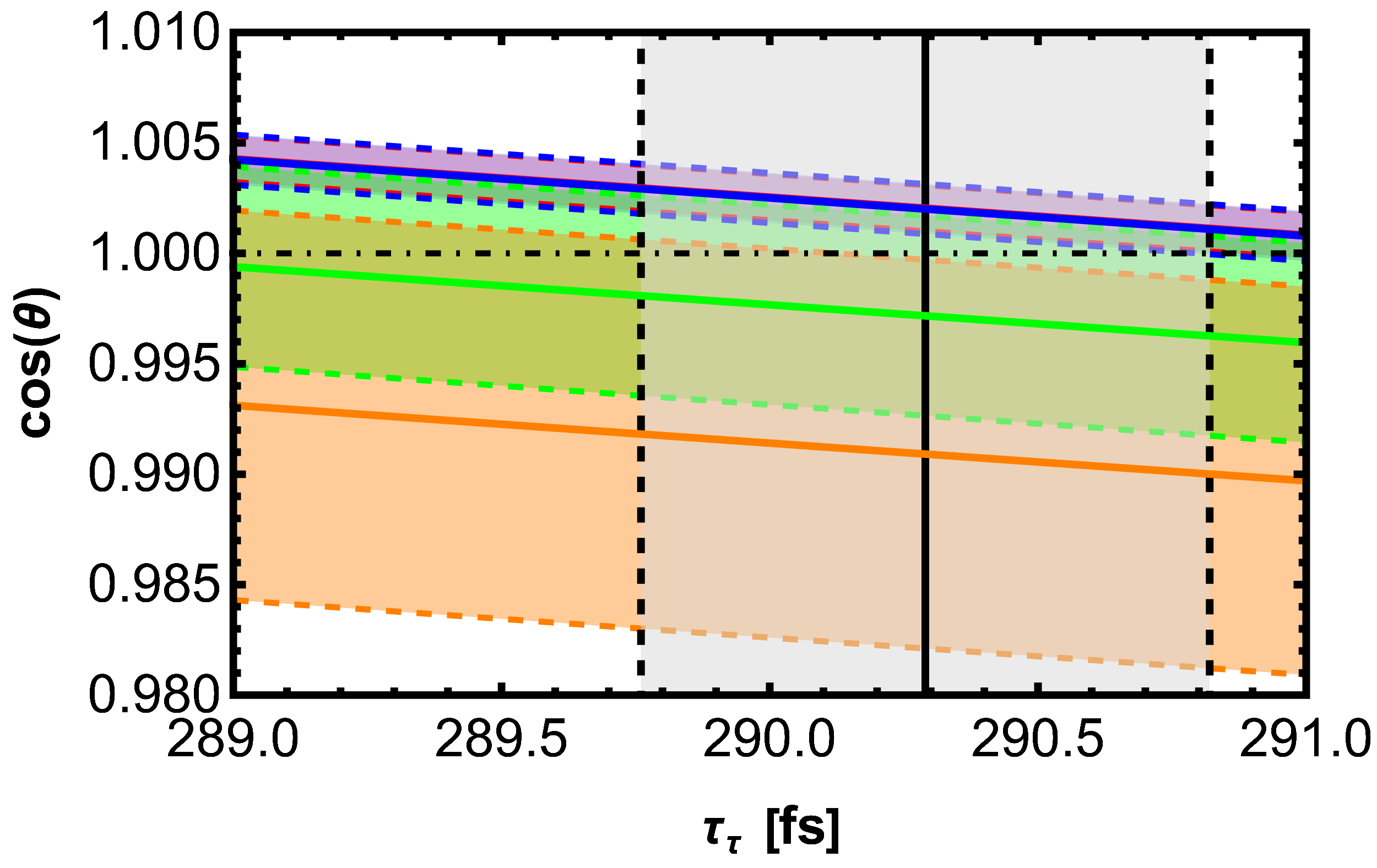
here we roughly estimated the errors by assuming they are all uncorrelated and distributed Gaussian. The leptonic decays all prefer unphysical values with cosθ>1\cos\theta>1 at the 1σ1\sigma level, the semi-hadronic decays, however, permit non-zero mixing angles at the 1σ1\sigma level. For the decay τπντ\tau\rightarrow\pi\nu_{\tau} we find the mixing angle at 1σ1\sigma

τπντ:|sinθ|12.2102at  1σ\tau\rightarrow\pi\nu_{\tau}:\qquad|\sin\theta|{\leq 12.2}\cdot 10^{-2}\quad\mathrm{at}\,\,1\sigma (57)

and for τKντ\tau\rightarrow K\nu_{\tau} the mixing angle

τKντ:|sinθ|=(13.511.3+5.4)102at  1σ.\tau\rightarrow K\nu_{\tau}:\qquad|\sin\theta|={\left(13.5_{-11.3}^{+5.4}\right)}\cdot 10^{-2}\quad\mathrm{at}\,\,1\sigma. (58)

In Fig. 12 we show the 1σ1\sigma band of the cosines of the mixing angle as a function of the τ\tau lifetime. Combining the semi-hadronic and leptonic decays yields cosθ=1.00168±0.00098\cos\theta=1.00168\pm 0.00098, while combining only the two semi-hadronic decays leads to cosθ=0.99582±0.00410\cos\theta=0.99582\pm 0.00410 corresponding to

τPντ,P=π,Kcombined:|sinθ|=(9.17.8+3.7)102at  1σ.\tau\rightarrow P\nu_{\tau},\quad P=\pi,K\,\,\mathrm{combined}:\qquad|\sin\theta|={\left(9.1_{-7.8}^{+3.7}\right)}\cdot 10^{-2}\quad\mathrm{at}\,\,1\sigma. (59)
Refer to caption
Figure 12: Cosine of the mixing angle vs. the τ\tau lifetime. The grey band is the 1σ1\sigma band of the world average of the τ\tau lifetime. The solid lines are the central values and the dashed lines delimit the 1σ1\sigma band. The bands from τντeν¯e\tau\rightarrow\nu_{\tau}e\bar{\nu}_{e} (blue) and τντμν¯μ\tau\rightarrow\nu_{\tau}\mu\bar{\nu}_{\mu} (red) overlap. the constraints from both τπντ\tau\rightarrow\pi\nu_{\tau} (green) and τKντ\tau\rightarrow K\nu_{\tau} (orange) fully comply with the measured τ\tau lifetime. The area under the dot-dashed line at cosθ=1\cos\theta=1 delimits the physically allowed region.


Taking the weighted average of the leptonic decays leads to cosθ=1.00203±0.00100\cos\theta=1.00203\pm 0.00100. These decays permit cosθ0.99901\cos\theta\geq 0.99901 at the 3σ3\sigma level leading to:

τντν¯=e,μcombined:|sinθ|4.4102at  3σ.\tau\to\nu_{\tau}\ell\bar{\nu}_{\ell}\quad\ell=e,\mu\,\,\mathrm{combined}:\qquad|\sin\theta|{\leq 4.4}\cdot 10^{-2}\quad\mathrm{at}\,\,3\sigma. (60)

4.5 Detecting HSN for mN<mτm_{N}<m_{\tau} from spectra

HSNs light enough to be produced in τ\tau decays are difficult to detect in branching ratios, because

Γ(τντY)+Γ(τNY)=ΓSM(τντY)+𝒪(mN2mτ2sin2θ)\Gamma(\tau\rightarrow\nu_{\tau}Y)+\Gamma(\tau\rightarrow NY)=\Gamma_{\mathrm{SM}}(\tau\rightarrow\nu_{\tau}Y)+\mathcal{O}\bigg(\frac{m_{N}^{2}}{m_{\tau}^{2}}\cdot\sin^{2}\theta\bigg) (61)

for mN<mτm_{N}<m_{\tau} and where YY is any final state. To this end one better employs precise measurements of the charged lepton energy spectrum

dΓ(τνν¯)dE=GF2mτ4Vν22π3F(xE,x,xν),\displaystyle\frac{d\Gamma(\tau\rightarrow\nu\ell\bar{\nu}_{\ell})}{dE_{\ell}}=\frac{G_{F}^{2}m_{\tau}^{4}V_{\nu}^{2}}{2\pi^{3}}F(x_{E},x_{\ell},x_{\nu}), (62)

here ν=ντ,N\nu=\nu_{\tau},N is either a SM or a sterile neutrino, xE=E/mτx_{E}=E_{\ell}/m_{\tau}, xi=mi/mτx_{i}=m_{i}/m_{\tau}, Vν=cosθV_{\nu}=\cos\theta for SM and Vν=sinθV_{\nu}=\sin\theta for sterile neutrinos, and

F(xE,x,xν)\displaystyle F(x_{E},x_{\ell},x_{\nu}) =xE2x2(12xE+x2xν2)26(12xE+x2)3\displaystyle=\frac{\sqrt{x_{E}^{2}-x_{\ell}^{2}}\big(1-2x_{E}+x_{\ell}^{2}-x_{\nu}^{2}\big)^{2}}{6\big(1-2x_{E}+x_{\ell}^{2}\big)^{3}} (63)
×[8xE32xE2(5+5x2+xν2)\displaystyle\hskip-56.9055pt\times\bigg[8x_{E}^{3}-2x_{E}^{2}(5+5x_{\ell}^{2}+x_{\nu}^{2})
+xE(3+10x2+3x4+3xν2(1+x2))2x2(1+x2+2xν2)].\displaystyle+x_{E}(3+10x_{\ell}^{2}+3x_{\ell}^{4}+3x_{\nu}^{2}(1+x_{\ell}^{2}))-2x_{\ell}^{2}(1+x_{\ell}^{2}+2x_{\nu}^{2})\bigg].

Since the experiment cannot distinguish between sterile and SM neutrino the measured lepton energy is

dΓlepexp.dE=\displaystyle\frac{d\Gamma^{\mathrm{exp.}}_{\mathrm{lep}}}{dE_{\ell}}= dΓ(τντν¯)dE+dΓ(τNν¯)dE\displaystyle\frac{d\Gamma(\tau\rightarrow\nu_{\tau}\ell\bar{\nu}_{\ell})}{dE_{\ell}}+\frac{d\Gamma(\tau\rightarrow N\ell\bar{\nu}_{\ell})}{dE_{\ell}} (64)
=\displaystyle= GF2mτ4Vν22π3[F(xE,x,xN)sin2θ+F(xE,x,0)cos2θ].\displaystyle\frac{G_{F}^{2}m_{\tau}^{4}V_{\nu}^{2}}{2\pi^{3}}\bigg[F(x_{E},x_{\ell},x_{N})\sin^{2}\theta+F(x_{E},x_{\ell},0)\cos^{2}\theta\bigg].
Refer to caption
Figure 13: Here we show FμNsin2θ+Fμ0cos2θ=F(Eμ/mτ,xμ,xN)sin2θ+F(Eμ/mτ,xμ,0)cos2θF_{\mu}^{N}\sin^{2}\theta+F_{\mu}^{0}\cos^{2}\theta=F(E_{\mu}/m_{\tau},x_{\mu},x_{N})\sin^{2}\theta+F(E_{\mu}/m_{\tau},x_{\mu},0)\cos^{2}\theta for =μ\ell=\mu, the black line corresponds to the SM case mN=0m_{N}=0, the mixing angle assumed here corresponds to sinθ=0.32\sin\theta=0.32.


The hadronic spectrum is derived analogously,

dΓ(τνX)ds=NcGF2mτ3Vν22(|Vud|2+|Vus|2)192π3S(mτ,mZ)G(x,xν),\displaystyle\frac{d\Gamma(\tau\rightarrow\nu X)}{ds}=N_{c}\frac{G_{F}^{2}m_{\tau}^{3}V_{\nu}^{2}\cdot 2(|V_{ud}|^{2}+|V_{us}|^{2})}{192\pi^{3}}S(m_{\tau},m_{Z})G\big(x,x_{\nu}\big), (65)

where S(mτ,mZ)=1.01907S(m_{\tau},m_{Z})=1.01907 Marciano and Sirlin (1988); Erler (2004) accounts for electroweak corrections, x=s/mτ2x=s/m_{\tau}^{2}, xν=mν/mτx_{\nu}=m_{\nu}/m_{\tau}, and

G(x,xν)\displaystyle G\big(x,x_{\nu}\big) =[(1+xν2x)(1+2x+xν2)4xν2]\displaystyle=\bigg[\bigg(1+x_{\nu}^{2}-x\bigg)\bigg(1+2x+x_{\nu}^{2}\bigg)-4x_{\nu}^{2}\bigg] (66)
×λ(1,x,xν2)12πImΠV1+0(mτ2x).\displaystyle\hskip 14.22636pt\times\sqrt{\lambda\big(1,x,x_{\nu}^{2}\big)}\cdot 12\pi\mathrm{Im}\,\Pi^{1+0}_{V}(m_{\tau}^{2}x).

As for the leptonic decay the measured quantity is the sum of SM and sterile neutrino contributions

dΓhadexp.ds=\displaystyle\frac{d\Gamma^{\mathrm{exp.}}_{\mathrm{had}}}{d{s}}= dΓ(τντX)ds+dΓ(τNX)ds\displaystyle\frac{d\Gamma(\tau\rightarrow\nu_{\tau}X)}{ds}+\frac{d\Gamma(\tau\rightarrow NX)}{ds} (67)
=\displaystyle= NcGF2mτ3Vν22(|Vud|2+|Vus|2)192π3S(mτ,mZ)\displaystyle N_{c}\frac{G_{F}^{2}m_{\tau}^{3}V_{\nu}^{2}\cdot 2(|V_{ud}|^{2}+|V_{us}|^{2})}{192\pi^{3}}S(m_{\tau},m_{Z})
×[G(x,xN)sin2θ+G(x,0)cos2θ].\displaystyle\times\bigg[G(x,x_{N})\sin^{2}\theta+G(x,0)\cos^{2}\theta\bigg].

In Figs. 13 and 14 we show the spectrum for the leptonic decay with =μ\ell=\mu in the final state and the hadronic spectrum, respectively, in both cases with sinθ=0.32\sin\theta=0.32. A HSN with a mass of mN=300 MeVm_{N}=$300\text{\,}\mathrm{MeV}$ leads to a significantly modified spectrum. The perturbative calculation of the hadronic spectrum can be compared to data for large s1s\gtrsim 1\,GeV. In addition, one can compare integrated spectra from s=0s=0 to a chosen smax1s_{\rm max}\gtrsim 1\,GeV, exploiting quark-hadron duality as described in Appendix B.

Refer to caption
Figure 14: The plot shows GhNsin2θ+Gh0cos2θ=G(s/mτ2,xN)sin2θ+G(s/mτ2,0)cos2θG_{h}^{N}\sin^{2}\theta+G_{h}^{0}\cos^{2}\theta=G(s/m_{\tau}^{2},x_{N})\sin^{2}\theta+G(s/m_{\tau}^{2},0)\cos^{2}\theta, the mixing angle is chosen to give sinθ=0.32\sin\theta=0.32.


4.6 Comparisons

It is interesting to compare the allowed values of the mixing angle with other experimental exclusions. Both ATLAS Aad and others (2024, 2025) and CMS Hayrapetyan et al. (2024); Hayrapetyan and others (2024b, a) have published upper and lower limits on the mixing angle. ATLAS performed an analysis for the HSN exclusively mixing with the τ\tau neutrino and is less competitive than CMS. The CMS experiment specifically looked at ντ\nu_{\tau}-NN mixing and is sensitive to HSN masses 1 GeVmN2.2 GeV$1\text{\,}\mathrm{GeV}$\leq m_{N}\lesssim$2.2\text{\,}\mathrm{GeV}$ and mN3 GeVm_{N}\geq$3\text{\,}\mathrm{GeV}$.

Below mN<3 GeVm_{N}<$3\text{\,}\mathrm{GeV}$ there are exclusion limits for NN-ντ\nu_{\tau} mixing from DELPHI Abreu and others (1997), ArgoNeuT Acciarri and others (2021), BABAR Lees and others (2023), and Belle Nayak and others (2024). In the mass range 0.4 GeVmN1.3 GeV$0.4\text{\,}\mathrm{GeV}$\leq m_{N}\leq$1.3\text{\,}\mathrm{GeV}$ ArgoNeuT and BABAR provide the strongest bounds. Beyond mN1.3 GeVm_{N}\geq$1.3\text{\,}\mathrm{GeV}$ DELPHI and CMS provide the strongest bounds, with the DELPHI bound being strongest for mN1.9 GeVm_{N}\gtrsim$1.9\text{\,}\mathrm{GeV}$. Furthermore, there are recasts of data from the CHARM Boiarska et al. (2021) and WA66 experiments Barouki et al. (2022). While originally these experiments were not understood to be sensitive to NN-ντ\nu_{\tau} mixing for HSN with masses mN1 GeVm_{N}\approx$1\text{\,}\mathrm{GeV}$, the recasts provide the tightest constraints up to mN=1.6 GeVm_{N}=$1.6\text{\,}\mathrm{GeV}$. Only the DELPHI experiment is sensitive to masses in the range 2.2 GeVmN<3 GeV$2.2\text{\,}\mathrm{GeV}$\lesssim m_{N}<$3\text{\,}\mathrm{GeV}$.

For 𝐦𝐍<𝐦τ\mathbf{m_{N}<m_{\tau}} we find the allowed range |VNτ|=|sinθ|0.2{|}V_{N\tau}{|}={|}\sin\theta{|}\lesssim 0.2 from the τ\tau lifetime for mN600 MeVm_{N}\approx$600\text{\,}\mathrm{MeV}$. In this mass regime our bound from τ\tau decay is not competitive, the strongest bound stems from the BABAR analysis, which finds |sinθ|2.49102{|}\sin\theta{|}\lesssim 2.49\cdot 10^{-2} Lees and others (2023), and the CHARM and WA66 recasts, |sinθ|1.73103{|}\sin\theta{|}\lesssim 1.73\cdot 10^{-3} Boiarska et al. (2021); Barouki et al. (2022), which, however, are more model-dependent as explained below.

For 𝐦𝐍>𝐦τ\mathbf{m_{N}>m_{\tau}} we find the mixing angle in Eq. (48) from the τ\tau lifetime. The semi-hadronic τ\tau decays exclude mixing angles for HSN masses mN>mτmPm_{N}>m_{\tau}-m_{P} where P=π,KP=\pi,K and lead to Eq. (57) for τπντ\tau\rightarrow\pi\nu_{\tau}, and Eq. (58) for τKντ\tau\rightarrow K\nu_{\tau}. In combination, the semi-hadronic decays lead to Eq. (59), valid for mN>mτmPm_{N}>m_{\tau}-m_{P}. Kobach and Dobbs (2015) Kobach and Dobbs (2015) have updated the bound of Ref. Helo et al. (2011). They used leptonic τ\tau decays to constrain the mixing angle for mN>mτm_{N}>m_{\tau} and derived the bound |sinθKD|7.07102{|}\sin\theta^{\mathrm{KD}}{|}\lesssim 7.07\cdot 10^{-2} at the 2σ\sim 2\sigma level. This is weaker than our bound obtained from leptonic τ\tau decays given in Eq. (60) at the 3σ3\sigma level. While our bounds obtained from semi-hadronic τ\tau decays (Eq. (59)) and the τ\tau lifetime (Eq. (48)) are weaker than the constraint from leptonic decays, they are less model-dependent as explained below. It is interesting to note that θ=0\theta=0 is ruled out by 1σ\sigma in Eq. (59). Bearing in mind that our error estimates do not consider correlations, these numbers may well indicate that better data may lead to evidence for θ0\theta\neq 0 in the foreseeable future.

The experiment most sensitive in the mass range 1.9 GeVmN3 GeV$1.9\text{\,}\mathrm{GeV}$\lesssim m_{N}\leq$3\text{\,}\mathrm{GeV}$ is the DELPHI experiment, determining sin2θDELPHI6105|sinθDELPHI|7.75103\sin^{2}\theta^{\mathrm{DELPHI}}\lesssim 6\cdot 10^{-5}\Rightarrow{|}\sin\theta^{\mathrm{DELPHI}}{|}\lesssim 7.75\cdot 10^{-3} for mN2 GeVm_{N}\approx$2\text{\,}\mathrm{GeV}$; the bound becomes weaker for smaller HSN masses Abreu and others (1997). The DELPHI experiment studied ZZ decays and was therefore sensitive to HSN and SM neutrinos of all flavors. However, they searched for the HSN through charged-current and neutral-current decays of HSN and derived the bound |sinθDELPHI|1.55102{|}\sin\theta^{\mathrm{DELPHI}}{|}\lesssim 1.55\cdot 10^{-2} from the non-observation of HSN decays into τ\tau leptons. The DELPHI bound is tighter than ours, but is also more model-dependent: While both our and the DELPHI study assume that NN only interacts with SM particles through NN-ντ\nu_{\tau} mixing, we do not assume anything on other interactions of NN. A heavy NN could be a mediator to a dark sector and possibly decay into lighter sterile neutrinos and/or dark bosons. In such scenarios the branching ratios of the decay modes studied by DELPHI will decrease and the bounds on |θ|{|}\theta{|} will become weaker and the same remark applies to the recasts of CHARM and WA66 data. For the same reason we also put less emphasis on the bounds on |θ|{|}\theta{|} in Eq. (60) found from leptonic decays. Unlike decays into final states with a single neutrino, leptonic τ\tau decays can be contaminated by decays into final states containing one or more massive dark bosons. Since the central values of the measured leptonic decay rates are higher than the SM predictions, we study this scenario in the next subsection.

Recently it was pointed out that indeed the LHC might already be capable of probing mixing angles for mixing of sterile neutrinos with τ\tau neutrinos far more efficiently Tireli et al. (2025). A reinterpretation of the existing LHC data would be highly interesting.

4.7 BSM scenarios with other light invisible particles

Leptonic τ\tau decays τντν¯\tau\rightarrow\nu_{\tau}\ell\bar{\nu}_{\ell} are interesting as there are two neutrinos produced in the final state: What is studied is τ+Emiss\tau\rightarrow\ell+E_{\mathrm{miss}} and the squared missing mass is much larger than zero, so that there can be contributions from Γ(τXdark)\Gamma(\tau\rightarrow\ell X_{\mathrm{dark}}) or Γ(τXdarkXdark)\Gamma(\tau\rightarrow\ell X_{\mathrm{dark}}X_{\mathrm{dark}}) with massive dark particles XdarkX_{\mathrm{dark}}. A natural candidate for an invisible boson emitted in a τ\tau decay is a majoron coupling to ντ\nu_{\tau} Chikashige et al. (1981); Gelmini and Roncadelli (1981); Barenboim and Nierste (2021).

We write ΓNP\Gamma_{\mathrm{NP}} for the dark contributions i.e. Γ(τ+Emiss)=Γ(τντν¯)+ΓNP\Gamma(\tau\rightarrow\ell+E_{\mathrm{miss}})=\Gamma(\tau\rightarrow\nu_{\tau}\ell\bar{\nu}_{\ell})+\Gamma_{\mathrm{NP}}. This constrains the new physics contribution to

ΓNP\displaystyle\Gamma_{\mathrm{NP}} =\displaystyle= (68)
Brexp.(τντeν¯e)Brexp.(τπντ)ΓSM(τπντ)ΓSM(τντeν¯e)=3.92±3.81 µeV\displaystyle\frac{\mathrm{Br}^{\mathrm{exp.}}(\tau\rightarrow\nu_{\tau}e\bar{\nu}_{e})}{\mathrm{Br}^{\mathrm{exp.}}(\tau\rightarrow\pi\nu_{\tau})}\Gamma_{\mathrm{SM}}(\tau\rightarrow\pi\nu_{\tau})-\Gamma_{\mathrm{SM}}(\tau\rightarrow\nu_{\tau}e\bar{\nu}_{e})=$3.92\pm 3.81\text{\,}\mathrm{\SIUnitSymbolMicro eV}$
ΓNP\displaystyle\Gamma_{\mathrm{NP}} =\displaystyle= (69)
Brexp.(τντμν¯μ)Brexp.(τπντ)ΓSM(τπντ)ΓSM(τντμν¯μ)=3.85±3.69 µeV,\displaystyle\frac{\mathrm{Br}^{\mathrm{exp.}}(\tau\rightarrow\nu_{\tau}\mu\bar{\nu}_{\mu})}{\mathrm{Br}^{\mathrm{exp.}}(\tau\rightarrow\pi\nu_{\tau})}\Gamma_{\mathrm{SM}}(\tau\rightarrow\pi\nu_{\tau})-\Gamma_{\mathrm{SM}}(\tau\rightarrow\nu_{\tau}\mu\bar{\nu}_{\mu})=$3.85\pm 3.69\text{\,}\mathrm{\SIUnitSymbolMicro eV}$,

where we set cosθ=1\cos\theta=1 because of the tight constraints on |sinθ||\sin\theta| found above.

5 Conclusions

In this paper, we have calculated the inclusive semi-hadronic charged-current decay width of HSNs up to 𝒪(αs4)\mathcal{O}(\alpha_{s}^{4}) in the strong coupling constant by using the known results of the electroweak gauge boson correlator which has been calculated up to the five-loop level. Decay rates into massless leptons can be trivially obtained from SM τ\tau decay rates, while Nτ+hadronsN\to\tau+\mbox{hadrons} decays involve new phase-space integrals. We derive analytic expressions in terms polylogarithms (up to 𝒪(αs3)\mathcal{O}(\alpha_{s}^{3})) and a series representation (valid for all calculated orders) for these rates. We then calculated the perturbative series and analyzed its stability in order to determine the sterile neutrino mass range for which the perturbative calculation is valid and robust theory predictions are possible. Reliable predictions for the semi-hadronic width are found for mN1.5 GeVm_{N}\geq$1.5\text{\,}\mathrm{GeV}$ for =e,μ\ell=e,\mu in the final state. For the final state with =τ\ell=\tau we find stability for mN3 GeVm_{N}\geq$3\text{\,}\mathrm{GeV}$. Our result can also be used for τN+hadrons\tau\to N+\mbox{hadrons} in the mass range mN600MeVm_{N}\lesssim 600\,\mbox{MeV}. In τ\tau decays the perturbative series is only stable after including the 𝒪(αs4)\mathcal{O}(\alpha_{s}^{4}) corrections.

We have further studied the impact of an NN-ντ\nu_{\tau} mixing angle θ\theta on the τ\tau lifetime. If NN is light enough to be produced in τ\tau decay, the SM decay amplitude is modified by a factor of cosθ\cos\theta and there is an additional τN+W\tau\rightarrow N+W^{*} mode with amplitude proportional to sinθ\sin\theta. We find the parameter space of mNm_{N} and θ\theta constrained by the τ\tau lifetime for HSN masses mN600 MeVm_{N}\lesssim$600\text{\,}\mathrm{MeV}$. Furthermore, we present expressions for the lepton energy spectrum in τνN\tau\to\ell\nu_{\ell}N and the hadron invariant mass spectrum in τN+hadrons\tau\to N+\mbox{hadrons}, which may be used to detect HSN effects in the future.

HSNs heavier than the τ\tau lepton may still leave imprints on observables through the cosine of the mixing angle. The lifetime analysis leads to |sinθ|11.8102|\sin\theta|\leq 11.8\cdot 10^{-2} at 1σ1\sigma in this case. For the four decays τντν¯\tau\rightarrow\nu_{\tau}\ell\bar{\nu}_{\ell} with =e,μ\ell=e,\mu and τPντ\tau\rightarrow P\nu_{\tau} with P=π,KP=\pi^{-},K^{-} we have compared the measured widths with the theoretical predictions. Only the data on the semi-hadronic decays permit a non-zero mixing angle and we derive the constraints |sinθ|12.2102|\sin\theta|\leq 12.2\cdot 10^{-2} at 1σ1\sigma from τπντ\tau\rightarrow\pi\nu_{\tau} and |sinθ|=(13.511.3+5.4)102|\sin\theta|=\left(13.5_{-11.3}^{+5.4}\right)\cdot 10^{-2} at 1σ1\sigma from τKντ\tau\rightarrow K\nu_{\tau}, respectively. Combining both semi-hadronic decays leads to |sinθ|=(9.17.8+3.7)102|\sin\theta|=\left(9.1_{-7.8}^{+3.7}\right)\cdot 10^{-2} at 1σ1\sigma. Our results are complementary to those from CMS, which constrain θ\theta for HSN masses above 3 GeV, and less model dependent than those of DELPHI below 3 GeV3\text{\,}\mathrm{GeV}. In another application of our calculation we have derived relative branching fractions between certain exclusive decays and the inclusive semi-hadronic decay and determined the fraction of Nπ+N\to\pi^{+}\ell^{-} decays of all N+hadronsN\to\ell^{-}+\mbox{hadrons} decays.

Finally we have derived a bound on the τ\tau decay width into final states containing one or more new invisible particles, for example majorons. These decays contaminate τν¯ντ\tau\to\ell\bar{\nu}_{\ell}\nu_{\tau}, whose decay rate is indeed a bit larger than the SM prediction. This finding calls for more precise experimental studies of the leptonic τ\tau decays.

Acknowledgements

This research was supported by the Deutsche Forschungsgemeinschaft (DFG, German Research Foundation) under grant 396021762 - TRR 257 for the Collaborative Research Center Particle Physics Phenomenology after the Higgs Discovery (P3H).

Appendix A QCD β\beta-Function

We use the β\beta-function with the following normalization

daμdlnμ2=β(aμ)=aμ2[β0+β1aμ+β2aμ2+],\frac{da_{\mu}}{d\ln\mu^{2}}=\beta(a_{\mu})=-a_{\mu}^{2}\bigg[\beta_{0}+\beta_{1}a_{\mu}+\beta_{2}a_{\mu}^{2}+...\bigg], (70)

where aμ=a(μ)=αs(μ)/πa_{\mu}=a(\mu)=\alpha_{s}(\mu)/\pi and with the coefficients βi\beta_{i} Czakon (2005); Chetyrkin et al. (2016):

β0\displaystyle\beta_{0} =14(1123nf),\displaystyle=\frac{1}{4}\left(11-\frac{2}{3}n_{f}\right), (71)
β1\displaystyle\beta_{1} =116(102383nf),\displaystyle=\frac{1}{16}\left(102-\frac{38}{3}n_{f}\right), (72)
β2\displaystyle\beta_{2} =164(28572503318nf+32554nf2).\displaystyle=\frac{1}{64}\left(\frac{2857}{2}-\frac{5033}{18}n_{f}+\frac{325}{54}n_{f}^{2}\right). (73)

Eq. (70) leads to

a(μ)=\displaystyle a(\mu)= a(μ0)a(μ0)2β0μμ0+a(μ0)3[β1μμ0+β02μμ02]\displaystyle a(\mu_{0})-a(\mu_{0})^{2}\beta_{0}\ell_{\mu\mu_{0}}+a(\mu_{0})^{3}\bigg[-\beta_{1}\ell_{\mu\mu_{0}}+\beta_{0}^{2}\ell_{\mu\mu_{0}}^{2}\bigg]
+a(μ0)4[β2μμ0+52β0β1μμ02β03μμ03]+𝒪(a(μ0)5),\displaystyle\hskip 28.45274pt+a(\mu_{0})^{4}\bigg[-\beta_{2}\ell_{\mu\mu_{0}}+\frac{5}{2}\beta_{0}\beta_{1}\ell_{\mu\mu_{0}}^{2}-\beta_{0}^{3}\ell_{\mu\mu_{0}}^{3}\bigg]+\mathcal{O}(a(\mu_{0})^{5}), (74)

where μμ0=ln(μ2μ02)\ell_{\mu\mu_{0}}=\ln\bigg(\frac{\mu^{2}}{\mu_{0}^{2}}\bigg).

Appendix B Contour Integration

In the framework of perturbative calculations it is possible to calculate scattering or decay processes into quarks. However, in an experiment only hadrons are detectable and not quarks. This poses a problem as hadrons at different masses would appear as resonances in e.g. cross-sections. These resonances however are not accounted for by perturbative calculations using quarks. This conundrum was resolved by Poggio, Quinn and Weinberg Poggio et al. (1976); they showed that a perturbative calculation smeared over a suitable energy range correctly averages over the resonances. This approach was then refined by showing that it is possible to transform the integration over the suitable energy range into an integration around a suitable complex contour Shankar (1977); Lam and Yan (1977). This was used for τ\tau decays Braaten et al. (1992); Braaten (1988), the integral in Eq. (22) can be rewritten in terms of a contour integration around a keyhole contour (see Fig. 15). Thus the decay width is proportional to the discontinuity over the branch cut along the positive real axis.

Refer to caption
Figure 15: Contour integration permitting to replace the integral over the resonance region by the integral over the large circle, which is far away from resonances. Thus, while the differential spectrum is not perturbatively calculable in that region, the integrated spectrum is found correctly in this way.

In this way the integral may be rewritten in the following way (setting the lepton mass to zero for brevity)

Γ(NX)\displaystyle\Gamma(N\rightarrow X\ell)\sim 12π0mN2𝑑s(1smN2)2[(1+2smN2)ImΠ(1+0)(s)2smN2ImΠ(0)(s)]\displaystyle 12\pi\int\limits_{0}^{m_{N}^{2}}ds\,\bigg(1-\frac{s}{m_{N}^{2}}\bigg)^{2}\bigg[\bigg(1+2\frac{s}{m_{N}^{2}}\bigg)\mathrm{Im}\Pi^{(1+0)}(s)-2\frac{s}{m_{N}^{2}}\mathrm{Im}\Pi^{(0)}(s)\bigg]
=6πis=mN2𝑑s(1smN2)2[(1+2smN2)Π(1+0)(s)2smN2Π(0)(s)],\displaystyle=6\pi i\oint\limits_{s=m_{N}^{2}}ds\,\bigg(1-\frac{s}{m_{N}^{2}}\bigg)^{2}\bigg[\bigg(1+2\frac{s}{m_{N}^{2}}\bigg)\Pi^{(1+0)}(s)-2\frac{s}{m_{N}^{2}}\Pi^{(0)}(s)\bigg],

the integral only depends on ss at the value of the mass of the decaying particle and so low energy effects are already accounted for in the decay width. Indeed in this way the inclusive decay width correctly averages over all possible resonances induced by the mesons.

Appendix C Easy-to-use Formulae for Phase-Space Integrals

For easier use we have expanded Eqs. (27), (28) as

I1approx.,T\displaystyle I_{1}^{\mathrm{approx.,\,T}} =2525x14+160x12+215x104324x8+343x6+(1522π2)x4\displaystyle=\frac{2}{525}x_{\ell}^{14}+\frac{1}{60}x_{\ell}^{12}+\frac{2}{15}x_{\ell}^{10}-\frac{43}{24}x_{\ell}^{8}+\frac{34}{3}x_{\ell}^{6}+\left(\frac{15}{2}-2\pi^{2}\right)x_{\ell}^{4} (75)
+103x21924+(x48x26)x4log(x)+𝒪(x16)\displaystyle+\frac{10}{3}x_{\ell}^{2}-\frac{19}{24}+\left(x_{\ell}^{4}-8x_{\ell}^{2}-6\right)x_{\ell}^{4}\log(x_{\ell})+\mathcal{O}(x_{\ell}^{16})
I2approx.,T\displaystyle I_{2}^{\mathrm{approx.,\,T}} =787110250x14+11800x12+217450x10+16(2π25)x8\displaystyle=-\frac{787}{110250}x_{\ell}^{14}+\frac{1}{1800}x_{\ell}^{12}+\frac{217}{450}x_{\ell}^{10}+\frac{1}{6}\left(2\pi^{2}-5\right)x_{\ell}^{8} (76)
+23(374π2)x62(12ζ(3)+3+π2)x4569x2+265144\displaystyle+\frac{2}{3}\left(37-4\pi^{2}\right)x_{\ell}^{6}-2\left(-12\zeta(3)+3+\pi^{2}\right)x_{\ell}^{4}-\frac{56}{9}x_{\ell}^{2}+\frac{265}{144}
(8x8+35x6+280x42100x2+16800)x6log(x)1050+𝒪(x16).\displaystyle-\frac{\left(8x_{\ell}^{8}+35x_{\ell}^{6}+280x_{\ell}^{4}-2100x_{\ell}^{2}+16800\right)x_{\ell}^{6}\log(x_{\ell})}{1050}+\mathcal{O}(x_{\ell}^{16}).

Additionally we have also fitted Eq. (27), (28) to polynomials (see Fig. 16)

I1approx.,P=\displaystyle I_{1}^{\mathrm{approx.,\,P}}= 1.27683x91.11042x810.3142x7+21.4421x69.05503x5\displaystyle 1.27683x_{\ell}^{9}-1.11042x_{\ell}^{8}-10.3142x_{\ell}^{7}+21.4421x_{\ell}^{6}-9.05503x_{\ell}^{5} (77)
6.19752x4+1.5042x3+3.24256x2+0.00309017x0.7917\displaystyle-6.19752x_{\ell}^{4}+1.5042x_{\ell}^{3}+3.24256x_{\ell}^{2}+0.00309017x_{\ell}-0.7917
I2approx.,P=\displaystyle I_{2}^{\mathrm{approx.,\,P}}= 4.83878x9+29.1877x853.4361x7+34.6139x67.13307x5\displaystyle-4.83878x_{\ell}^{9}+29.1877x_{\ell}^{8}-53.4361x_{\ell}^{7}+34.6139x_{\ell}^{6}-7.13307x_{\ell}^{5} (78)
+6.63816x40.720101x36.14877x20.00323628x+1.84032\displaystyle+6.63816x_{\ell}^{4}-0.720101x_{\ell}^{3}-6.14877x_{\ell}^{2}-0.00323628x_{\ell}+1.84032
Refer to caption
Figure 16: The absolute error |1Iiapprox.,T/P/Ii||1-I_{i}^{\mathrm{approx.,\,T/P}}/I_{i}| of the approximations in Eqs. (7578). The solid red and blue curves correspond to the Taylor expansion and the dashed blue and red curves are the polynomial fit. The dashed black line indicates the 1%1\% level. For x0.8x_{\ell}\lesssim 0.8 both approximations have uncertainties |1Iiapprox.,T/P/Ii|<1%|1-I_{i}^{\mathrm{approx.,\,T/P}}/I_{i}|<1\%.

Appendix D Integrated Spectrum

Here we present the analytical solutions of the integral

Ik(x2,xmax)=0xmax𝑑x((1+x2x)(1+2x+x2)4x2)λ(1,x,x2)lnk(x),I_{k}(x_{\ell}^{2},x_{\mathrm{max}})=\int\limits_{0}^{x_{\mathrm{max}}}dx\,\bigg((1+x_{\ell}^{2}-x)(1+2x+x_{\ell}^{2})-4x_{\ell}^{2}\bigg)\sqrt{\lambda(1,x,x_{\ell}^{2})}\ln^{k}(x), (79)

for k<3k<3.

Refer to caption
Figure 17: Here IkXIkI_{k}^{X}-I_{k} is plotted for two different values of x=0.2x_{\ell}=0.2 (closed line) and x=0.5x_{\ell}=0.5 (dashed line). The vertically dashed line lies at the end of the spectrum of the dashed curves i.e. (10.5)2=0.25(1-0.5)^{2}=0.25. At the end of the spectrum the IiXIi=0I_{i}^{X}-I_{i}=0

In Fig. 17 the Ik(x2,xmax)Ik(x2,(1x)2)I_{k}(x_{\ell}^{2},x_{\mathrm{max}})-I_{k}(x_{\ell}^{2},(1-x_{\ell})^{2}) are shown.

The Ik(x2,xmax)Ik(x2,(1x)2)I_{k}(x_{\ell}^{2},x_{\mathrm{max}})-I_{k}(x_{\ell}^{2},(1-x_{\ell})^{2}), which we denote as IkXIkI_{k}^{X}-I_{k} and use xmax=x^x_{\mathrm{max}}=\hat{x} as a shorthand notation, take the following form

I0XI0=\displaystyle I_{0}^{X}-I_{0}= 12((x^2+7)x2(x^+7)x4+x6\displaystyle\frac{1}{2}\bigg(-\bigg(\hat{x}^{2}+7\bigg)x_{\ell}^{2}-(\hat{x}+7)x_{\ell}^{4}+x_{\ell}^{6} (80)
+(x^1)2(x^+1))(x^(x+1)2)Xr24x4ArcTanh(Xr)\displaystyle\hskip 28.45274pt+(\hat{x}-1)^{2}(\hat{x}+1)\bigg)\bigg(\hat{x}-(x_{\ell}+1)^{2}\bigg)X_{r}-24x_{\ell}^{4}\mathrm{ArcTanh}(X_{r})
I1XI1=\displaystyle I_{1}^{X}-I_{1}= 12x4(ΔLi2(X2x)ΔLi2(X2)+ΔLi2(1Xr2))\displaystyle 12x_{\ell}^{4}\bigg(\Delta\mathrm{Li}_{2}\bigg(-\frac{X_{-}}{2x_{\ell}}\bigg)-\Delta\mathrm{Li}_{2}\bigg(\frac{X_{-}}{2}\bigg)+\Delta\mathrm{Li}_{2}\bigg(\frac{1-X_{r}}{2}\bigg)\bigg) (81)
+124Xr(x^(x+1)2)\displaystyle+\frac{1}{24}X_{r}\bigg(\hat{x}-(x_{\ell}+1)^{2}\bigg)
×(3x^3+12((x^2+7)x2(x^+7)x4+x6+(x^1)2(x^+1))ln(x^)\displaystyle\times\bigg(-3\hat{x}^{3}+12\big(-(\hat{x}^{2}+7)x_{\ell}^{2}-(\hat{x}+7)x_{\ell}^{4}+x_{\ell}^{6}+(\hat{x}-1)^{2}(\hat{x}+1)\big)\ln(\hat{x})
+5(x^2+x^)+(x^(5x^+4)+85)x2+5(x^+17)x419x619)\displaystyle\hskip 28.45274pt+5(\hat{x}^{2}+\hat{x})+(\hat{x}(5\hat{x}+4)+85)x_{\ell}^{2}+5(\hat{x}+17)x_{\ell}^{4}-19x_{\ell}^{6}-19\bigg)
+(8x26x4(4ln(x^)+2ln(1Xr2)4ln(2)+2))\displaystyle+\bigg(-8x_{\ell}^{2}-6x_{\ell}^{4}\bigg(4\ln(\hat{x})+2\ln\bigg(1-X_{r}^{2}\bigg)-4\ln(2)+2)\bigg)
8x6+x8+1)ArcTanh(Xr)\displaystyle\hskip 28.45274pt-8x_{\ell}^{6}+x_{\ell}^{8}+1\bigg)\mathrm{ArcTanh}(X_{r})
(8x2+24x4ln(x)8x6+x81)ArcTanh(Xr1+x1x)\displaystyle-\bigg(8x_{\ell}^{2}+24x_{\ell}^{4}\ln(x_{\ell})-8x_{\ell}^{6}+x_{\ell}^{8}-1\bigg)\mathrm{ArcTanh}\bigg(-X_{r}\frac{1+x_{\ell}}{1-x_{\ell}}\bigg)
I2XI2=\displaystyle I_{2}^{X}-I_{2}= Xr[((x^2+7)x3(x^1)(x^2+3)x2+(x^+3)x6+(x^+7)x5\displaystyle X_{r}\bigg[\bigg(\big(\hat{x}^{2}+7\big)x_{\ell}^{3}-(\hat{x}-1)\big(\hat{x}^{2}+3\big)x_{\ell}^{2}+(\hat{x}+3)x_{\ell}^{6}+(\hat{x}+7)x_{\ell}^{5} (82)
+(73x^)x4(x^1)2(x^+1)x+12(x^1)3(x^+1)x82x7)ln2(x^)\displaystyle+(7-3\hat{x})x_{\ell}^{4}-(\hat{x}-1)^{2}(\hat{x}+1)x_{\ell}+\frac{1}{2}(\hat{x}-1)^{3}(\hat{x}+1)-\frac{x_{\ell}^{8}}{2}-x_{\ell}^{7}\bigg)\ln^{2}(\hat{x})
+(112(3x^4+8x^324x^+19)+(2x^112)x656(x^+17)x5\displaystyle+\bigg(\frac{1}{12}\big(-3\hat{x}^{4}+8\hat{x}^{3}-24\hat{x}+19\big)+\bigg(-2\hat{x}-\frac{11}{2}\bigg)x_{\ell}^{6}-\frac{5}{6}(\hat{x}+17)x_{\ell}^{5}
+16(38x^85)x4+16(x^(5x^+4)85)x3\displaystyle+\frac{1}{6}(38\hat{x}-85)x_{\ell}^{4}+\frac{1}{6}(-\hat{x}(5\hat{x}+4)-85)x_{\ell}^{3}
+16(x^(x^(4x^3)+38)33)x2+16(x^(x^(3x^5)5)+19)x\displaystyle+\frac{1}{6}(\hat{x}(\hat{x}(4\hat{x}-3)+38)-33)x_{\ell}^{2}+\frac{1}{6}(\hat{x}(\hat{x}(3\hat{x}-5)-5)+19)x_{\ell}
+19x812+19x76)ln(x^)+1144(9x^432x^3+288x^265)\displaystyle+\frac{19x_{\ell}^{8}}{12}+\frac{19x_{\ell}^{7}}{6}\bigg)\ln(\hat{x})+\frac{1}{144}\bigg(9\hat{x}^{4}-32\hat{x}^{3}+288\hat{x}-265\bigg)
+(2x^+11324)x6+2372(x^+41)x5+172(943446x^)x4\displaystyle+\bigg(2\hat{x}+\frac{113}{24}\bigg)x_{\ell}^{6}+\frac{23}{72}(\hat{x}+41)x_{\ell}^{5}+\frac{1}{72}(943-446\hat{x})x_{\ell}^{4}
+172(x^(23x^+28)+943)x3+172(x^((916x^)x^446)+339)x2\displaystyle+\frac{1}{72}(\hat{x}(23\hat{x}+28)+943)x_{\ell}^{3}+\frac{1}{72}(\hat{x}((9-16\hat{x})\hat{x}-446)+339)x_{\ell}^{2}
+172(x^((239x^)x^+23)265)x265x8144265x772]\displaystyle+\frac{1}{72}(\hat{x}((23-9\hat{x})\hat{x}+23)-265)x_{\ell}-\frac{265x_{\ell}^{8}}{144}-\frac{265x_{\ell}^{7}}{72}\bigg]
+x4[16𝒫(0,7,5,0)ArcTanh2(Xr)\displaystyle+x_{\ell}^{4}\bigg[-16\mathcal{P}_{(0,7,5,0)}\mathrm{ArcTanh}^{2}(X_{r})
+24ln(1Xr2)(Li2(XxX+)Li2(XX+x))\displaystyle+24\ln\bigg(1-X_{r}^{2}\bigg)\bigg(\text{Li}_{2}\bigg(-\frac{X_{-}x_{\ell}}{X_{+}}\bigg)-\text{Li}_{2}\bigg(-\frac{X_{-}}{X_{+}x_{\ell}}\bigg)\bigg)
+24Li3(XX+x)24Li3(XxX+)+48Li3(XXr1)\displaystyle+24\text{Li}_{3}\bigg(-\frac{X_{-}}{X_{+}x_{\ell}}\bigg)-24\text{Li}_{3}\bigg(-\frac{X_{-}x_{\ell}}{X_{+}}\bigg)+48\text{Li}_{3}\bigg(-\frac{X_{-}}{X_{r}-1}\bigg)
+48Li3(Xr+1(Xr1)x+1)+24Li3((Xr+1)xXr1)\displaystyle+48\text{Li}_{3}\bigg(\frac{X_{r}+1}{(X_{r}-1)x_{\ell}}+1\bigg)+24\text{Li}_{3}\bigg(-\frac{(X_{r}+1)x_{\ell}}{X_{r}-1}\bigg)
+24Li3(xXrxXr+1)+30ArcTanh(Xr)48ζ(3)]\displaystyle+24\text{Li}_{3}\bigg(\frac{x_{\ell}-X_{r}x_{\ell}}{X_{r}+1}\bigg)+30\mathrm{ArcTanh}(X_{r})-48\zeta(3)\bigg]
+16x8𝒫(0,19,0,3)+x6𝒫(0,463,2,4)+x2𝒫(0,2,463,4)\displaystyle+\frac{1}{6}x_{\ell}^{8}\mathcal{P}_{(0,19,0,-3)}+x_{\ell}^{6}\mathcal{P}_{(0,-\frac{46}{3},-2,4)}+x_{\ell}^{2}\mathcal{P}_{(0,2,\frac{46}{3},-4)}
+ln(x)[x8𝒫(0,1,3,0)8x6𝒫(0,1,3,0)12x4𝒫(π2,0,2,1)\displaystyle+\ln(x_{\ell})\bigg[x_{\ell}^{8}\mathcal{P}_{(0,1,3,0)}-8x_{\ell}^{6}\mathcal{P}_{(0,1,3,0)}-12x_{\ell}^{4}\mathcal{P}_{(\pi^{2},0,2,-1)}
+ln(x^)(12x4(4ArcTanh(Xr)+1)+2x816x6)\displaystyle+\ln(\hat{x})\bigg(-12x_{\ell}^{4}\bigg(4\mathrm{ArcTanh}(X_{r})+1\bigg)+2x_{\ell}^{8}-16x_{\ell}^{6}\bigg)
12x4ln2(x^)+48x4ln(X)ArcTanh(Xr)\displaystyle-12x_{\ell}^{4}\ln^{2}(\hat{x})+48x_{\ell}^{4}\ln(X_{-})\mathrm{ArcTanh}(X_{r})
+ln(X+)(24x4(2ln(1Xr2)+2ArcTanh(Xr)1)4x8+32x6)\displaystyle+\ln(X_{+})\bigg(-24x_{\ell}^{4}\bigg(2\ln\bigg(1-X_{r}^{2}\bigg)+2\mathrm{ArcTanh}(X_{r})-1\bigg)-4x_{\ell}^{8}+32x_{\ell}^{6}\bigg)
+48x4ln2(X+)+96x4ArcTanh(Xr)ln(1x)\displaystyle+48x_{\ell}^{4}\ln^{2}(X_{+})+96x_{\ell}^{4}\mathrm{ArcTanh}(X_{r})\ln(1-x_{\ell})
16x2ArcTanh(Xr)+2ArcTanh(Xr)]\displaystyle-16x_{\ell}^{2}\mathrm{ArcTanh}(X_{r})+2\mathrm{ArcTanh}(X_{r})\bigg]
+ln2(x)(12x4(2ln(X+)𝒫(0,2,0,0))+p(x)2)12x4ln3(x)\displaystyle+\ln^{2}(x_{\ell})\bigg(12x_{\ell}^{4}(2\ln(X_{+})-\mathcal{P}_{(0,2,0,0)})+\frac{p(x_{\ell})}{2}\bigg)-12x_{\ell}^{4}\ln^{3}(x_{\ell})
+ln(x^)[x8𝒫(1912,2,0,0)+x6𝒫(263,16,0,0)+x2𝒫(263,0,16,0)+𝒫(1912,0,2,0)\displaystyle+\ln(\hat{x})\bigg[x_{\ell}^{8}\mathcal{P}_{(\frac{19}{12},-2,0,0)}+x_{\ell}^{6}\mathcal{P}_{(-\frac{26}{3},16,0,0)}+x_{\ell}^{2}\mathcal{P}_{(\frac{26}{3},0,-16,0)}+\mathcal{P}_{(-\frac{19}{12},0,2,0)}
24x4(Li2(XX+x)Li2(XxX+)\displaystyle-24x_{\ell}^{4}\bigg(\text{Li}_{2}\bigg(-\frac{X_{-}}{X_{+}x_{\ell}}\bigg)-\text{Li}_{2}\bigg(-\frac{X_{-}x_{\ell}}{X_{+}}\bigg)
+2ArcTanh(Xr)2+ArcTanh(Xr))2p(x)(ln(X+)ln(x+1))]\displaystyle+2\mathrm{ArcTanh}(X_{r})^{2}+\mathrm{ArcTanh}(X_{r})\bigg)-2p(x_{\ell})(\ln(X_{+})-\ln(x_{\ell}+1))\bigg]
+12ln2(x^)(p(x)48x4ArcTanh(Xr))+2ln2(X+)p(x)\displaystyle+\frac{1}{2}\ln^{2}(\hat{x})\bigg(p(x_{\ell})-48x_{\ell}^{4}\mathrm{ArcTanh}(X_{r})\bigg)+2\ln^{2}(X_{+})p(x_{\ell})
+ln(X+)[(x81)𝒫(196,2,2,0)(x41)x2𝒫(523,16,16,0)\displaystyle+\ln(X_{+})\bigg[\bigg(x_{\ell}^{8}-1\bigg)\mathcal{P}_{(-\frac{19}{6},2,2,0)}-\bigg(x_{\ell}^{4}-1\bigg)x_{\ell}^{2}\mathcal{P}_{(-\frac{52}{3},16,16,0)}
+48x4(Li2(XX+x)Li2(XxX+))\displaystyle+48x_{\ell}^{4}\bigg(\text{Li}_{2}\bigg(-\frac{X_{-}}{X_{+}x_{\ell}}\bigg)-\text{Li}_{2}\bigg(-\frac{X_{-}x_{\ell}}{X_{+}}\bigg)\bigg)
4p(x)ln(x+1)+144x4ArcTanh2(Xr)]\displaystyle-4p(x_{\ell})\ln(x_{\ell}+1)+144x_{\ell}^{4}\mathrm{ArcTanh}^{2}(X_{r})\bigg]
+48x4ArcTanh2(Xr)ln(X)\displaystyle+48x_{\ell}^{4}\mathrm{ArcTanh}^{2}(X_{r})\ln(X_{-})
+ln(1x)[8x4(6ΔLi2(X1Xr)+6ΔLi2(X2x)\displaystyle+\ln(1-x_{\ell})\bigg[8x_{\ell}^{4}\bigg(6\Delta\mathrm{Li}_{2}\bigg(\frac{X_{-}}{1-X_{r}}\bigg)+6\Delta\mathrm{Li}_{2}\bigg(-\frac{X_{-}}{2x_{\ell}}\bigg)
6ΔLi2(12(Xr1)(x+1))\displaystyle-6\Delta\mathrm{Li}_{2}\bigg(-\frac{1}{2}(X_{r}-1)(x_{\ell}+1)\bigg)
12Li2(Xr+12)+6ln(X)(ln(Xr+1)+ln(x+12))\displaystyle-12\text{Li}_{2}\bigg(\frac{X_{r}+1}{2}\bigg)+6\ln(X_{-})\bigg(\ln(X_{r}+1)+\ln\bigg(\frac{x_{\ell}+1}{2}\bigg)\bigg)
6ln(X+)(ln(1Xr2)+ln(x+1))+6ln(2)ln(1Xr2)\displaystyle-6\ln(X_{+})\bigg(\ln\bigg(\frac{1-X_{r}}{2}\bigg)+\ln(x_{\ell}+1)\bigg)+6\ln(2)\ln\bigg(1-X_{r}^{2}\bigg)
6ln2(Xr+1)+12ArcTanh2(Xr)+π26ln2(2))\displaystyle-6\ln^{2}(X_{r}+1)+12\mathrm{ArcTanh}^{2}(X_{r})+\pi^{2}-6\ln^{2}(2)\bigg)
+2p(x)(ln(x^)2ln(X+)+ln(1Xr2))]\displaystyle+2p(x_{\ell})\bigg(\ln(\hat{x})-2\ln(X_{+})+\ln\bigg(1-X_{r}^{2}\bigg)\bigg)\bigg]
+16(𝒫(0,0,19,3)+p(x)(6Li2(XX+x)+6Li2(XxX+)\displaystyle+\frac{1}{6}\bigg(\mathcal{P}_{(0,0,-19,3)}+p(x_{\ell})\bigg(6\text{Li}_{2}\bigg(-\frac{X_{-}}{X_{+}x_{\ell}}\bigg)+6\text{Li}_{2}\bigg(-\frac{X_{-}x_{\ell}}{X_{+}}\bigg)
+12ln(1Xr2)ln(x+1)+π2))\displaystyle+12\ln\bigg(1-X_{r}^{2}\bigg)\ln(x_{\ell}+1)+\pi^{2}\bigg)\bigg)
+Li2(X1Xr)q(x)Li2(X+1+Xr)q+(x)\displaystyle+\mathrm{Li}_{2}\bigg(\frac{X_{-}}{1-X_{r}}\bigg)q_{-}(x_{\ell})-\mathrm{Li}_{2}\bigg(\frac{X_{+}}{1+X_{r}}\bigg)q_{+}(x_{\ell})

where the IiI_{i} are given in Eq. (26-28) and Xr=(x^(1x)2)/(x^(1+x)2)X_{r}=\sqrt{(\hat{x}-(1-x_{\ell})^{2})/(\hat{x}-(1+x_{\ell})^{2})}. We defined the following abbreviations

X±\displaystyle X_{\pm} =(1x)±Xr(1+x),\displaystyle=(1-x_{\ell})\pm X_{r}(1+x_{\ell}), (83)
𝒫a,b,c,d\displaystyle\mathcal{P}_{a,b,c,d} =a+bln(1Xr)+cln(1+Xr)+dln2(1Xr2)\displaystyle=a+b\ln(1-X_{r})+c\ln(1+X_{r})+d\ln^{2}(1-X_{r}^{2}) (84)
ΔLin(f(Xr))\displaystyle\Delta\mathrm{Li}_{n}(f(X_{r})) =Lin(f(Xr))Lin(f(Xr))\displaystyle=\mathrm{Li}_{n}(f(X_{r}))-\mathrm{Li}_{n}(f(-X_{r})) (85)
p(x)\displaystyle p(x_{\ell}) =18x2+8x6x8\displaystyle=1-8x_{\ell}^{2}+8x_{\ell}^{6}-x_{\ell}^{8} (86)
q±(x)\displaystyle q_{\pm}(x_{\ell}) =18x212x48x6+x8\displaystyle=1-8x_{\ell}^{2}-12x_{\ell}^{4}-8x_{\ell}^{6}+x_{\ell}^{8} (87)
24x4ln(x^)±24x4ln(x^(1Xr2)X+2)\displaystyle\hskip 56.9055pt-24x_{\ell}^{4}\ln(\hat{x})\pm 24x_{\ell}^{4}\ln\bigg(\frac{\hat{x}(1-X_{r}^{2})}{X_{+}^{2}}\bigg)

where f(Xr)f(X_{r}) is an arbitrary function depending on XrX_{r}.

Using Eq. (79) we plot the integrated decay width Γcut\Gamma_{\mathrm{cut}} defined as

Γcut(NX)=\displaystyle\Gamma_{\mathrm{cut}}(N\rightarrow\ell X)= NcGF2mN5|VN|2192π3\displaystyle N_{c}\frac{G_{F}^{2}m_{N}^{5}|V_{N\ell}|^{2}}{192\pi^{3}} (88)
×2(|Vud|2+|Vus|2)[I0c0,1+amNc1,1I0\displaystyle\times 2(|V_{ud}|^{2}+|V_{us}|^{2})\bigg[I_{0}c_{0,1}+a_{m_{N}}c_{1,1}I_{0}
+amN2(c2,1I0+2c2,2I1)\displaystyle+a_{m_{N}}^{2}\big(c_{2,1}I_{0}+2c_{2,2}I_{1}\big)
+amN3(c3,1I0+2c3,2I1(π2I03I2)c3,3)\displaystyle+a_{m_{N}}^{3}\big(c_{3,1}I_{0}+2c_{3,2}I_{1}-(\pi^{2}I_{0}-3I_{2})c_{3,3}\big)
+amN4(c4,1I0Q+2c4,2I1\displaystyle+a_{m_{N}}^{4}\big(c_{4,1}I_{0}^{Q}+2c_{4,2}I_{1}
(π2I03I2)c4,3(4π2I14I3)c4,4)]\displaystyle\hphantom{a_{\mu}^{4}}-(\pi^{2}I_{0}-3I_{2})c_{4,3}-(4\pi^{2}I_{1}-4I_{3})c_{4,4}\big)\bigg]

where Ik=Ik(x2,xmax)I_{k}=I_{k}(x_{\ell}^{2},x_{\mathrm{max}}), see Fig. 18.

Refer to caption
Figure 18: Integrated spectrum ΓNX(xmax)\Gamma_{N}^{X}(x_{\mathrm{max}}). The width is plotted with a mixing angle of VN=103V_{N\ell}=10^{-3} and the lepton is a tau =τ\ell=\tau. In the full curve the mass of the HSN is mN=4 GeVm_{N}=$4\text{\,}\mathrm{GeV}$ whereas in the dashed curve it is mN=3 GeVm_{N}=$3\text{\,}\mathrm{GeV}$; the dashed vertical line marks the endpoint of the integrated spectrum for the dashed red curve.

References

  • [FNAL/MILC 14A] A. Bazavov et al. (2014) Charmed and light pseudoscalar meson decay constants from four-flavor lattice QCD with physical light quarks. Phys.Rev. D90 (7), pp. 074509. External Links: Document, 1407.3772 Cited by: Table 1.
  • G. Aad et al. (2024) Search for heavy right-handed Majorana neutrinos in the decay of top quarks produced in proton-proton collisions at s=13  TeV with the ATLAS detector. Phys. Rev. D 110 (11), pp. 112004. External Links: 2408.05000, Document Cited by: §4.6.
  • G. Aad et al. (2025) Search for heavy neutral leptons in decays of W bosons using leptonic and semi-leptonic displaced vertices in s\sqrt{s} = 13 TeV pp collisions with the ATLAS detector. JHEP 07, pp. 196. External Links: 2503.16213, Document Cited by: §4.6.
  • P. Abreu et al. (1997) Search for neutral heavy leptons produced in Z decays. Z. Phys. C 74, pp. 57–71. Note: [Erratum: Z.Phys.C 75, 580 (1997)] External Links: Document Cited by: §4.6, §4.6.
  • R. Acciarri et al. (2021) New Constraints on Tau-Coupled Heavy Neutral Leptons with Masses mN=280–970  MeV. Phys. Rev. Lett. 127 (12), pp. 121801. External Links: 2106.13684, Document Cited by: §4.6.
  • S. L. Adler (1974) Some Simple Vacuum Polarization Phenomenology: e+eHadronse^{+}e^{-}\to\mathrm{Hadrons}: The muonic-atom x-Ray Discrepancy and gμ2g_{\mu}-2. Phys. Rev. D 10, pp. 3714. External Links: Document Cited by: §2.2.
  • C. Alexandrou et al. (2021) Ratio of kaon and pion leptonic decay constants with Nf=2+1+1N_{f}=2+1+1 Wilson-clover twisted-mass fermions. Phys. Rev. D 104 (7), pp. 074520. External Links: 2104.06747, Document Cited by: Table 1, Table 1.
  • Y. Aoki et al. (2024) FLAG Review 2024. External Links: 2411.04268 Cited by: Figure 9, Table 1, Table 1.
  • M. A. Arroyo-Ureña, G. Hernández-Tomé, G. López-Castro, P. Roig, and I. Rosell (2021) Radiative corrections to τ\tauπ\pi(K)ν\nuτ\tau[γ\gamma]: A reliable new physics test. Phys. Rev. D 104 (9), pp. L091502. External Links: 2107.04603, Document Cited by: §4.4.
  • M. A. Arroyo-Ureña, G. Hernández-Tomé, G. López-Castro, P. Roig, and I. Rosell (2022) One-loop determination of τ\tauπ\pi(K)ν\nuτ [γ\gamma] branching ratios and new physics tests. JHEP 02, pp. 173. External Links: 2112.01859, Document Cited by: §4.4.
  • T. Asaka, S. Blanchet, and M. Shaposhnikov (2005) The ν\nuMSM, dark matter and neutrino masses. Physics Letters B 631 (4), pp. 151–156. External Links: ISSN 0370-2693, Link, Document Cited by: §1.
  • T. Asaka and M. Shaposhnikov (2005) The ν\nuMSM, dark matter and baryon asymmetry of the universe. Physics Letters B 620 (1–2), pp. 17–26. External Links: ISSN 0370-2693, Link, Document Cited by: §1.
  • A. Atre, T. Han, S. Pascoli, and B. Zhang (2009) The search for heavy majorana neutrinos. Journal of High Energy Physics 2009 (05), pp. 030–030. External Links: ISSN 1029-8479, Link, Document Cited by: §2.1.
  • P. A. Baikov, K. G. Chetyrkin, J. H. Kühn, and J. Rittinger (2012) Complete 𝒪(αs4)\mathcal{O}(\alpha_{s}^{4}) QCD Corrections to Hadronic ZZ Decays. Phys. Rev. Lett. 108, pp. 222003. External Links: Document, Link Cited by: §2.2.
  • P. A. Baikov, K. G. Chetyrkin, and J. H. Kuhn (2008) Order α4(s)\alpha^{4}(s) QCD Corrections to ZZ and τ\tau Decays. Phys. Rev. Lett. 101, pp. 012002. External Links: 0801.1821, Document Cited by: §1, §2.2, §2.2, §4.1, §4.1.
  • S. Banerjee et al. (2024) Averages of bb-hadron, cc-hadron, and τ\tau-lepton properties as of 2023. External Links: 2411.18639 Cited by: 44, §4.4, Table 1, Table 1, Table 1, Table 1.
  • G. Barenboim and U. Nierste (2021) Modified majoron model for cosmological anomalies. Phys. Rev. D 104 (2), pp. 023013. External Links: 2005.13280, Document Cited by: §4.7.
  • R. Barouki, G. Marocco, and S. Sarkar (2022) Blast from the past II: Constraints on heavy neutral leptons from the BEBC WA66 beam dump experiment. SciPost Phys. 13, pp. 118. External Links: 2208.00416, Document Cited by: §4.6, §4.6.
  • A. Bazavov et al. (2018) BB- and DD-meson leptonic decay constants from four-flavor lattice QCD. Phys. Rev. D 98 (7), pp. 074512. External Links: 1712.09262, Document Cited by: Figure 9, Table 1.
  • C. Becchi, S. Narison, E. de Rafael, and F. J. Yndurain (1981) Light Quark Masses in Quantum Chromodynamics and Chiral Symmetry Breaking. Z. Phys. C 8, pp. 335. External Links: Document Cited by: §2.2.
  • M. Beneke and M. Jamin (2008) αs\alpha_{s} And the τ\tau hadronic width: fixed-order, contour- improved and higher-order perturbation theory. Journal of High Energy Physics 2008 (09), pp. 044–044. External Links: ISSN 1029-8479, Link, Document Cited by: §1, §2.2, §2.2.
  • F. U. Bernlochner, M. Fedele, T. Kretz, U. Nierste, and M. T. Prim (2025) Model independent bounds on heavy sterile neutrinos from the angular distribution of BDνB\to D^{*}\ell\nu decays. JHEP 01, pp. 040. External Links: 2410.11945, Document Cited by: §1.
  • I. Boiarska, A. Boyarsky, O. Mikulenko, and M. Ovchynnikov (2021) Constraints from the CHARM experiment on heavy neutral leptons with tau mixing. Phys. Rev. D 104 (9), pp. 095019. External Links: 2107.14685, Document Cited by: §4.6, §4.6.
  • K. Bondarenko, A. Boyarsky, D. Gorbunov, and O. Ruchayskiy (2018) Phenomenology of GeV-scale heavy neutral leptons. Journal of High Energy Physics 2018 (11). External Links: ISSN 1029-8479, Link, Document Cited by: §1, §2.1.
  • E. Braaten, S. Narison, and A. Pich (1992) QCD analysis of the tau hadronic width. Nuclear Physics B 373 (3), pp. 581–612. External Links: ISSN 0550-3213, Document, Link Cited by: Appendix B, §2.2, §2.2, §3.
  • E. Braaten (1988) QCD predictions for the decay of the τ\tau lepton. Phys. Rev. Lett. 60, pp. 1606–1609. External Links: Document, Link Cited by: Appendix B.
  • N. Carrasco et al. (2015) Leptonic decay constants fK,fD,f_{K},f_{D}, and fDsf_{{D}_{s}} with Nf=2+1+1N_{f}=2+1+1 twisted-mass lattice QCD. Phys. Rev. D 91 (5), pp. 054507. External Links: 1411.7908, Document Cited by: Figure 9, Table 1, Table 1.
  • W. Celmaster and R. J. Gonsalves (1980) Analytic calculation of higher-order quantum-chromodynamic corrections in e+e{e}^{+}{e}^{-} annihilation. Phys. Rev. Lett. 44, pp. 560–564. External Links: Document, Link Cited by: §2.2.
  • K. G. Chetyrkin, A. L. Kataev, and F. V. Tkachov (1979) Higher Order Corrections to σtot(e+eHadrons)\sigma_{\mathrm{tot}}(e^{+}e^{-}\rightarrow\mathrm{Hadrons}) in Quantum Chromodynamics. Phys. Lett. B 85, pp. 277–279. External Links: Document Cited by: §2.2.
  • K. G. Chetyrkin, J. H. Kuhn, and M. Steinhauser (2000) RunDec: A Mathematica package for running and decoupling of the strong coupling and quark masses. Comput. Phys. Commun. 133, pp. 43–65. External Links: hep-ph/0004189, Document Cited by: Figure 4.
  • K.G. Chetyrkin, J.H. Kühn, and A.A. Pivovarov (1998) Determining the strange quark mass in cabibbo-suppressed tau lepton decays. Nuclear Physics B 533 (1–3), pp. 473–493. External Links: ISSN 0550-3213, Link, Document Cited by: §2.2.
  • K. Chetyrkin, P. Baikov, and J. Kühn (2016) The β\beta-function of Quantum Chromodynamics and the effective Higgs-gluon-gluon coupling in five-loop order. PoS LL2016, pp. 010. External Links: Document Cited by: Appendix A.
  • Y. Chikashige, R. N. Mohapatra, and R. D. Peccei (1981) Are There Real Goldstone Bosons Associated with Broken Lepton Number?. Phys. Lett. B 98, pp. 265–268. External Links: Document Cited by: §4.7.
  • V. Cirigliano, D. Díaz-Calderón, A. Falkowski, M. González-Alonso, and A. Rodríguez-Sánchez (2022) Semileptonic tau decays beyond the Standard Model. JHEP 04, pp. 152. External Links: 2112.02087, Document Cited by: §4.4.
  • V. Cirigliano and I. Rosell (2007) The Standard Model prediction for Re/μ(π,K)R_{e/\mu}^{(\pi,K)}. Phys. Rev. Lett. 99, pp. 231801. External Links: 0707.3439, Document Cited by: §4.4.
  • G. Cvetič and C. S. Kim (2016) Rare decays of BB mesons via on-shell sterile neutrinos. Phys. Rev. D 94, pp. 053001. External Links: Document, Link Cited by: §2.1.
  • M. Czakon (2005) The four-loop qcd β\beta-function and anomalous dimensions. Nuclear Physics B 710 (1–2), pp. 485–498. External Links: ISSN 0550-3213, Link, Document Cited by: Appendix A.
  • S. Davidson and A. Ibarra (2002) A Lower bound on the right-handed neutrino mass from leptogenesis. Phys. Lett. B 535, pp. 25–32. External Links: hep-ph/0202239, Document Cited by: §1.
  • M. Dine and J. Sapirstein (1979) Higher-order quantum chromodynamic corrections in e+e{e}^{+}{e}^{-} annihilation. Phys. Rev. Lett. 43, pp. 668–671. External Links: Document, Link Cited by: §2.2.
  • R. J. Dowdall, C. T. H. Davies, G. P. Lepage, and C. McNeile (2013) VusV_{us} from π\pi and KK decay constants in full lattice QCD with physical uu, dd, ss and cc quarks. Phys. Rev. D 88, pp. 074504. External Links: 1303.1670, Document Cited by: Table 1, Table 1.
  • J. Ellis (2017) TikZ-Feynman: Feynman diagrams with TikZ. Comput. Phys. Commun. 210, pp. 103–123. External Links: 1601.05437, Document Cited by: Figure 1.
  • J. Erler and M. Luo (2003) Precision determination of heavy quark masses and the strong coupling constant. Phys. Lett. B 558, pp. 125–131. External Links: hep-ph/0207114, Document Cited by: 45.
  • J. Erler (1999) Calculation of the QED coupling α^(MZ)\hat{\alpha}(M_{Z}) in the modified minimal subtraction scheme. Phys. Rev. D 59, pp. 054008. External Links: hep-ph/9803453, Document Cited by: Table 1.
  • J. Erler (2004) Electroweak radiative corrections to semileptonic tau decays. Rev. Mex. Fis. 50, pp. 200–202. External Links: hep-ph/0211345 Cited by: §4.5, Table 1.
  • M. Fukugita and T. Yanagida (1986) Baryogenesis Without Grand Unification. Phys. Lett. B 174, pp. 45–47. External Links: Document Cited by: §1.
  • M. Gell-Mann, P. Ramond, and R. Slansky (1979) Complex Spinors and Unified Theories. Conf. Proc. C 790927, pp. 315–321. External Links: 1306.4669 Cited by: §1.
  • G. B. Gelmini and M. Roncadelli (1981) Left-Handed Neutrino Mass Scale and Spontaneously Broken Lepton Number. Phys. Lett. B 99, pp. 411–415. External Links: Document Cited by: §4.7.
  • S. L. Glashow (1980) The Future of Elementary Particle Physics. NATO Sci. Ser. B 61, pp. 687. External Links: Document Cited by: §1.
  • D. Gorbunov and M. Shaposhnikov (2007) How to find neutral leptons of the ν\nu MSM?. Journal of High Energy Physics 2007 (10), pp. 015–015. External Links: ISSN 1029-8479, Link, Document Cited by: §2.1.
  • S. G. Gorishnii, A. L. Kataev, and S. A. Larin (1988) Next-To-Leading 𝒪(αs3)\mathcal{O}(\alpha_{s}^{3}) QCD Correction to σtot(e+eHadrons)\sigma_{\mathrm{tot}}(e^{+}e^{-}\rightarrow\mathrm{Hadrons}): Analytical Calculation and Estimation of the Parameter Lambda (MS). Phys. Lett. B 212, pp. 238–244. External Links: Document Cited by: §2.2.
  • S. G. Gorishnii, A. L. Kataev, and S. A. Larin (1991) The O(αs3)O(\alpha^{3}_{s})-corrections to σtot(e+ehadrons)\sigma_{tot}(e^{+}e^{-}\rightarrow\mathrm{hadrons}) and Γ(τντ+hadrons)\Gamma(\tau^{-}\rightarrow\nu_{\tau}+\mathrm{hadrons}) in QCD. Phys. Lett. B 259, pp. 144–150. External Links: Document Cited by: §2.2.
  • V. Gribanov, S. Kovalenko, and I. Schmidt (2001) Sterile neutrinos in tau lepton decays. Nuclear Physics B 607 (1–2), pp. 355–368. External Links: ISSN 0550-3213, Link, Document Cited by: §2.1.
  • A. Hayrapetyan, A. Tumasyan, W. Adam, J. W. Andrejkovic, T. Bergauer, S. Chatterjee, K. Damanakis, M. Dragicevic, P. S. Hussain, M. Jeitler, N. Krammer, A. Li, D. Liko, I. Mikulec, J. Schieck, R. Schöfbeck, D. Schwarz, M. Sonawane, S. Templ, W. Waltenberger, C.-E. Wulz, M. R. Darwish, T. Janssen, P. Van Mechelen, E. S. Bols, J. D’Hondt, S. Dansana, A. De Moor, M. Delcourt, H. El Faham, S. Lowette, I. Makarenko, D. Müller, A. R. Sahasransu, S. Tavernier, M. Tytgat, G. P. Van Onsem, S. Van Putte, D. Vannerom, B. Clerbaux, A. K. Das, G. De Lentdecker, L. Favart, P. Gianneios, D. Hohov, J. Jaramillo, A. Khalilzadeh, K. Lee, M. Mahdavikhorrami, A. Malara, S. Paredes, L. Pétré, N. Postiau, L. Thomas, M. Vanden Bemden, C. Vander Velde, P. Vanlaer, M. De Coen, D. Dobur, Y. Hong, J. Knolle, L. Lambrecht, G. Mestdach, K. Mota Amarilo, C. Rendón, A. Samalan, K. Skovpen, N. Van Den Bossche, J. van der Linden, L. Wezenbeek, A. Benecke, A. Bethani, G. Bruno, C. Caputo, C. Delaere, I. S. Donertas, A. Giammanco, K. Jaffel, Sa. Jain, V. Lemaitre, J. Lidrych, P. Mastrapasqua, K. Mondal, T. T. Tran, S. Wertz, G. A. Alves, E. Coelho, C. Hensel, T. Menezes De Oliveira, A. Moraes, P. Rebello Teles, M. Soeiro, W. L. Aldá Júnior, M. Alves Gallo Pereira, M. Barroso Ferreira Filho, H. Brandao Malbouisson, W. Carvalho, J. Chinellato, E. M. Da Costa, G. G. Da Silveira, D. De Jesus Damiao, S. Fonseca De Souza, R. Gomes De Souza, J. Martins, C. Mora Herrera, L. Mundim, H. Nogima, J. P. Pinheiro, A. Santoro, A. Sznajder, M. Thiel, A. Vilela Pereira, C. A. Bernardes, L. Calligaris, T. R. Fernandez Perez Tomei, E. M. Gregores, P. G. Mercadante, S. F. Novaes, B. Orzari, S. S. Padula, A. Aleksandrov, G. Antchev, R. Hadjiiska, P. Iaydjiev, M. Misheva, M. Shopova, G. Sultanov, A. Dimitrov, L. Litov, B. Pavlov, P. Petkov, A. Petrov, E. Shumka, S. Keshri, S. Thakur, T. Cheng, T. Javaid, L. Yuan, Z. Hu, J. Liu, K. Yi, G. M. Chen, H. S. Chen, M. Chen, F. Iemmi, C. H. Jiang, A. Kapoor, H. Liao, Z.-A. Liu, R. Sharma, J. N. Song, J. Tao, C. Wang, J. Wang, Z. Wang, H. Zhang, A. Agapitos, Y. Ban, A. Levin, C. Li, Q. Li, Y. Mao, S. J. Qian, X. Sun, D. Wang, H. Yang, L. Zhang, C. Zhou, Z. You, N. Lu, G. Bauer, X. Gao, D. Leggat, H. Okawa, Z. Lin, C. Lu, M. Xiao, C. Avila, D. A. Barbosa Trujillo, A. Cabrera, C. Florez, J. Fraga, J. A. Reyes Vega, J. Mejia Guisao, F. Ramirez, M. Rodriguez, J. D. Ruiz Alvarez, D. Giljanovic, N. Godinovic, D. Lelas, A. Sculac, M. Kovac, T. Sculac, P. Bargassa, V. Brigljevic, B. K. Chitroda, D. Ferencek, S. Mishra, A. Starodumov, T. Susa, A. Attikis, K. Christoforou, S. Konstantinou, J. Mousa, C. Nicolaou, F. Ptochos, P. A. Razis, H. Rykaczewski, H. Saka, A. Stepennov, M. Finger, M. Finger, A. Kveton, E. Ayala, E. Carrera Jarrin, H. Abdalla, Y. Assran, M. A. Mahmoud, Y. Mohammed, K. Ehataht, M. Kadastik, T. Lange, S. Nandan, C. Nielsen, J. Pata, M. Raidal, L. Tani, C. Veelken, H. Kirschenmann, K. Osterberg, M. Voutilainen, S. Bharthuar, E. Brücken, F. Garcia, K. T. S. Kallonen, R. Kinnunen, T. Lampén, K. Lassila-Perini, S. Lehti, T. Lindén, L. Martikainen, M. Myllymäki, M. m. Rantanen, H. Siikonen, E. Tuominen, J. Tuominiemi, P. Luukka, H. Petrow, M. Besancon, F. Couderc, M. Dejardin, D. Denegri, J. L. Faure, F. Ferri, S. Ganjour, P. Gras, G. Hamel de Monchenault, V. Lohezic, J. Malcles, J. Rander, A. Rosowsky, M. Ö. Sahin, A. Savoy-Navarro, P. Simkina, M. Titov, M. Tornago, C. Baldenegro Barrera, F. Beaudette, A. Buchot Perraguin, P. Busson, A. Cappati, C. Charlot, M. Chiusi, F. Damas, O. Davignon, A. De Wit, B. A. Fontana Santos Alves, S. Ghosh, A. Gilbert, R. Granier de Cassagnac, A. Hakimi, B. Harikrishnan, L. Kalipoliti, G. Liu, J. Motta, M. Nguyen, C. Ochando, L. Portales, R. Salerno, J. B. Sauvan, Y. Sirois, A. Tarabini, E. Vernazza, A. Zabi, A. Zghiche, J.-L. Agram, J. Andrea, D. Apparu, D. Bloch, J.-M. Brom, E. C. Chabert, C. Collard, S. Falke, U. Goerlach, C. Grimault, R. Haeberle, A.-C. Le Bihan, M. Meena, G. Saha, M. A. Sessini, P. Van Hove, S. Beauceron, B. Blancon, G. Boudoul, N. Chanon, J. Choi, D. Contardo, P. Depasse, C. Dozen, H. El Mamouni, J. Fay, S. Gascon, M. Gouzevitch, C. Greenberg, G. Grenier, B. Ille, I. B. Laktineh, M. Lethuillier, L. Mirabito, S. Perries, A. Purohit, M. Vander Donckt, P. Verdier, J. Xiao, I. Bagaturia, I. Lomidze, Z. Tsamalaidze, V. Botta, L. Feld, K. Klein, M. Lipinski, D. Meuser, A. Pauls, N. Röwert, M. Teroerde, S. Diekmann, A. Dodonova, N. Eich, D. Eliseev, F. Engelke, J. Erdmann, M. Erdmann, P. Fackeldey, B. Fischer, T. Hebbeker, K. Hoepfner, F. Ivone, A. Jung, M. y. Lee, L. Mastrolorenzo, F. Mausolf, M. Merschmeyer, A. Meyer, S. Mukherjee, D. Noll, A. Novak, F. Nowotny, A. Pozdnyakov, Y. Rath, W. Redjeb, F. Rehm, H. Reithler, U. Sarkar, V. Sarkisovi, A. Schmidt, A. Sharma, J. L. Spah, A. Stein, F. Torres Da Silva De Araujo, L. Vigilante, S. Wiedenbeck, S. Zaleski, C. Dziwok, G. Flügge, W. Haj Ahmad, T. Kress, A. Nowack, O. Pooth, A. Stahl, T. Ziemons, A. Zotz, H. Aarup Petersen, M. Aldaya Martin, J. Alimena, S. Amoroso, Y. An, S. Baxter, M. Bayatmakou, H. Becerril Gonzalez, O. Behnke, A. Belvedere, S. Bhattacharya, F. Blekman, K. Borras, A. Campbell, A. Cardini, C. Cheng, F. Colombina, S. Consuegra Rodríguez, G. Correia Silva, M. De Silva, G. Eckerlin, D. Eckstein, L. I. Estevez Banos, O. Filatov, E. Gallo, A. Geiser, A. Giraldi, G. Greau, V. Guglielmi, M. Guthoff, A. Hinzmann, A. Jafari, L. Jeppe, N. Z. Jomhari, B. Kaech, M. Kasemann, C. Kleinwort, R. Kogler, M. Komm, D. Krücker, W. Lange, D. Leyva Pernia, K. Lipka, W. Lohmann, R. Mankel, I.-A. Melzer-Pellmann, M. Mendizabal Morentin, A. B. Meyer, G. Milella, A. Mussgiller, L. P. Nair, A. Nürnberg, Y. Otarid, J. Park, D. Pérez Adán, E. Ranken, A. Raspereza, B. Ribeiro Lopes, J. Rübenach, A. Saggio, M. Scham, S. Schnake, P. Schütze, C. Schwanenberger, D. Selivanova, K. Sharko, M. Shchedrolosiev, R. E. Sosa Ricardo, D. Stafford, F. Vazzoler, A. Ventura Barroso, R. Walsh, Q. Wang, Y. Wen, K. Wichmann, L. Wiens, C. Wissing, Y. Yang, A. Zimermmane Castro Santos, A. Albrecht, S. Albrecht, M. Antonello, S. Bein, L. Benato, M. Bonanomi, P. Connor, M. Eich, K. El Morabit, Y. Fischer, A. Fröhlich, C. Garbers, E. Garutti, A. Grohsjean, M. Hajheidari, J. Haller, H. R. Jabusch, G. Kasieczka, P. Keicher, R. Klanner, W. Korcari, T. Kramer, V. Kutzner, F. Labe, J. Lange, A. Lobanov, C. Matthies, A. Mehta, L. Moureaux, M. Mrowietz, A. Nigamova, Y. Nissan, A. Paasch, K. J. Pena Rodriguez, T. Quadfasel, B. Raciti, M. Rieger, D. Savoiu, J. Schindler, P. Schleper, M. Schröder, J. Schwandt, M. Sommerhalder, H. Stadie, G. Steinbrück, A. Tews, M. Wolf, S. Brommer, M. Burkart, E. Butz, T. Chwalek, A. Dierlamm, A. Droll, N. Faltermann, M. Giffels, A. Gottmann, F. Hartmann, R. Hofsaess, M. Horzela, U. Husemann, J. Kieseler, M. Klute, R. Koppenhöfer, J. M. Lawhorn, M. Link, A. Lintuluoto, S. Maier, S. Mitra, M. Mormile, Th. Müller, M. Neukum, M. Oh, M. Presilla, G. Quast, K. Rabbertz, B. Regnery, N. Shadskiy, I. Shvetsov, H. J. Simonis, M. Toms, N. Trevisani, R. Ulrich, R. F. Von Cube, M. Wassmer, S. Wieland, F. Wittig, R. Wolf, X. Zuo, G. Anagnostou, G. Daskalakis, A. Kyriakis, A. Papadopoulos, A. Stakia, P. Kontaxakis, G. Melachroinos, A. Panagiotou, I. Papavergou, I. Paraskevas, N. Saoulidou, K. Theofilatos, E. Tziaferi, K. Vellidis, I. Zisopoulos, G. Bakas, T. Chatzistavrou, G. Karapostoli, K. Kousouris, I. Papakrivopoulos, E. Siamarkou, G. Tsipolitis, A. Zacharopoulou, K. Adamidis, I. Bestintzanos, I. Evangelou, C. Foudas, C. Kamtsikis, P. Katsoulis, P. Kokkas, P. G. Kosmoglou Kioseoglou, N. Manthos, I. Papadopoulos, J. Strologas, M. Bartók, C. Hajdu, D. Horvath, F. Sikler, V. Veszpremi, M. Csanád, K. Farkas, M. M. A. Gadallah, Á. Kadlecsik, P. Major, K. Mandal, G. Pásztor, A. J. Rádl, G. I. Veres, P. Raics, B. Ujvari, G. Zilizi, G. Bencze, S. Czellar, J. Molnar, Z. Szillasi, T. Csorgo, F. Nemes, T. Novak, J. Babbar, S. Bansal, S. B. Beri, V. Bhatnagar, G. Chaudhary, S. Chauhan, N. Dhingra, A. Kaur, A. Kaur, H. Kaur, M. Kaur, S. Kumar, K. Sandeep, T. Sheokand, J. B. Singh, A. Singla, A. Ahmed, A. Bhardwaj, A. Chhetri, B. C. Choudhary, A. Kumar, A. Kumar, M. Naimuddin, K. Ranjan, S. Saumya, S. Baradia, S. Barman, S. Bhattacharya, S. Dutta, S. Dutta, S. Sarkar, M. M. Ameen, P. K. Behera, S. C. Behera, S. Chatterjee, P. Jana, P. Kalbhor, J. R. Komaragiri, D. Kumar, L. Panwar, P. R. Pujahari, N. R. Saha, A. Sharma, A. K. Sikdar, S. Verma, S. Dugad, M. Kumar, G. B. Mohanty, P. Suryadevara, A. Bala, S. Banerjee, R. M. Chatterjee, R. K. Dewanjee, M. Guchait, Sh. Jain, S. Karmakar, S. Kumar, G. Majumder, K. Mazumdar, S. Parolia, A. Thachayath, S. Bahinipati, C. Kar, D. Maity, P. Mal, T. Mishra, V. K. Muraleedharan Nair Bindhu, K. Naskar, A. Nayak, P. Sadangi, P. Saha, S. K. Swain, S. Varghese, D. Vats, S. Acharya, A. Alpana, S. Dube, B. Gomber, B. Kansal, A. Laha, B. Sahu, S. Sharma, H. Bakhshiansohi, E. Khazaie, M. Zeinali, S. Chenarani, S. M. Etesami, M. Khakzad, M. Mohammadi Najafabadi, M. Grunewald, M. Abbrescia, R. Aly, A. Colaleo, D. Creanza, B. D’Anzi, N. De Filippis, M. De Palma, A. Di Florio, W. Elmetenawee, L. Fiore, G. Iaselli, M. Louka, G. Maggi, M. Maggi, I. Margjeka, V. Mastrapasqua, S. My, S. Nuzzo, A. Pellecchia, A. Pompili, G. Pugliese, R. Radogna, G. Ramirez-Sanchez, D. Ramos, A. Ranieri, L. Silvestris, F. M. Simone, Ü. Sözbilir, A. Stamerra, R. Venditti, P. Verwilligen, A. Zaza, G. Abbiendi, C. Battilana, D. Bonacorsi, L. Borgonovi, R. Campanini, P. Capiluppi, F. R. Cavallo, M. Cuffiani, G. M. Dallavalle, T. Diotalevi, F. Fabbri, A. Fanfani, D. Fasanella, P. Giacomelli, L. Giommi, C. Grandi, L. Guiducci, S. Lo Meo, L. Lunerti, S. Marcellini, G. Masetti, F. L. Navarria, A. Perrotta, F. Primavera, A. M. Rossi, T. Rovelli, G. P. Siroli, S. Costa, A. Di Mattia, R. Potenza, A. Tricomi, C. Tuve, P. Assiouras, G. Barbagli, G. Bardelli, B. Camaiani, A. Cassese, R. Ceccarelli, V. Ciulli, C. Civinini, R. D’Alessandro, E. Focardi, T. Kello, G. Latino, P. Lenzi, M. Lizzo, M. Meschini, S. Paoletti, A. Papanastassiou, G. Sguazzoni, L. Viliani, L. Benussi, S. Bianco, S. Meola, D. Piccolo, P. Chatagnon, F. Ferro, E. Robutti, S. Tosi, A. Benaglia, G. Boldrini, F. Brivio, F. Cetorelli, F. De Guio, M. E. Dinardo, P. Dini, S. Gennai, R. Gerosa, A. Ghezzi, P. Govoni, L. Guzzi, M. T. Lucchini, M. Malberti, S. Malvezzi, A. Massironi, D. Menasce, L. Moroni, M. Paganoni, D. Pedrini, B. S. Pinolini, S. Ragazzi, T. Tabarelli de Fatis, D. Zuolo, S. Buontempo, A. Cagnotta, F. Carnevali, N. Cavallo, A. De Iorio, F. Fabozzi, A. O. M. Iorio, L. Lista, P. Paolucci, B. Rossi, C. Sciacca, R. Ardino, P. Azzi, N. Bacchetta, D. Bisello, P. Bortignon, A. Bragagnolo, R. Carlin, P. Checchia, T. Dorigo, S. Fantinel, F. Fanzago, U. Gasparini, E. Lusiani, M. Margoni, F. Marini, A. T. Meneguzzo, M. Migliorini, J. Pazzini, P. Ronchese, R. Rossin, G. Strong, M. Tosi, A. Triossi, S. Ventura, H. Yarar, M. Zanetti, P. Zotto, A. Zucchetta, G. Zumerle, S. Abu Zeid, C. Aimè, A. Braghieri, S. Calzaferri, D. Fiorina, P. Montagna, V. Re, C. Riccardi, P. Salvini, I. Vai, P. Vitulo, S. Ajmal, G. M. Bilei, D. Ciangottini, L. Fanò, M. Magherini, G. Mantovani, V. Mariani, M. Menichelli, F. Moscatelli, A. Rossi, A. Santocchia, D. Spiga, T. Tedeschi, P. Asenov, P. Azzurri, G. Bagliesi, R. Bhattacharya, L. Bianchini, T. Boccali, E. Bossini, D. Bruschini, R. Castaldi, M. A. Ciocci, M. Cipriani, V. D’Amante, R. Dell’Orso, S. Donato, A. Giassi, F. Ligabue, D. Matos Figueiredo, A. Messineo, M. Musich, F. Palla, A. Rizzi, G. Rolandi, S. Roy Chowdhury, T. Sarkar, A. Scribano, P. Spagnolo, R. Tenchini, G. Tonelli, N. Turini, A. Venturi, P. G. Verdini, P. Barria, M. Campana, F. Cavallari, L. Cunqueiro Mendez, D. Del Re, E. Di Marco, M. Diemoz, F. Errico, E. Longo, P. Meridiani, J. Mijuskovic, G. Organtini, F. Pandolfi, R. Paramatti, C. Quaranta, S. Rahatlou, C. Rovelli, F. Santanastasio, L. Soffi, N. Amapane, R. Arcidiacono, S. Argiro, M. Arneodo, N. Bartosik, R. Bellan, A. Bellora, C. Biino, C. Borca, N. Cartiglia, M. Costa, R. Covarelli, N. Demaria, L. Finco, M. Grippo, B. Kiani, F. Legger, F. Luongo, C. Mariotti, L. Markovic, S. Maselli, A. Mecca, E. Migliore, M. Monteno, R. Mulargia, M. M. Obertino, G. Ortona, L. Pacher, N. Pastrone, M. Pelliccioni, M. Ruspa, F. Siviero, V. Sola, A. Solano, A. Staiano, C. Tarricone, D. Trocino, G. Umoret, E. Vlasov, S. Belforte, V. Candelise, M. Casarsa, F. Cossutti, K. De Leo, G. Della Ricca, S. Dogra, J. Hong, C. Huh, B. Kim, D. H. Kim, J. Kim, H. Lee, S. W. Lee, C. S. Moon, Y. D. Oh, M. S. Ryu, S. Sekmen, Y. C. Yang, M. S. Kim, G. Bak, P. Gwak, H. Kim, D. H. Moon, E. Asilar, D. Kim, T. J. Kim, J. A. Merlin, S. Choi, S. Han, B. Hong, K. Lee, K. S. Lee, S. Lee, J. Park, S. K. Park, J. Yoo, J. Goh, S. Yang, H. S. Kim, Y. Kim, S. Lee, J. Almond, J. H. Bhyun, J. Choi, W. Jun, J. Kim, S. Ko, H. Kwon, H. Lee, J. Lee, J. Lee, B. H. Oh, S. B. Oh, H. Seo, U. K. Yang, I. Yoon, W. Jang, D. Y. Kang, Y. Kang, S. Kim, B. Ko, J. S. H. Lee, Y. Lee, I. C. Park, Y. Roh, I. J. Watson, S. Ha, H. D. Yoo, M. Choi, M. R. Kim, H. Lee, Y. Lee, I. Yu, T. Beyrouthy, Y. Maghrbi, K. Dreimanis, A. Gaile, G. Pikurs, A. Potrebko, M. Seidel, V. Veckalns, N. R. Strautnieks, M. Ambrozas, A. Juodagalvis, A. Rinkevicius, G. Tamulaitis, N. Bin Norjoharuddeen, I. Yusuff, Z. Zolkapli, J. F. Benitez, A. Castaneda Hernandez, H. A. Encinas Acosta, L. G. Gallegos Maríñez, M. León Coello, J. A. Murillo Quijada, A. Sehrawat, L. Valencia Palomo, G. Ayala, H. Castilla-Valdez, H. Crotte Ledesma, E. De La Cruz-Burelo, I. Heredia-De La Cruz, R. Lopez-Fernandez, C. A. Mondragon Herrera, A. Sánchez Hernández, C. Oropeza Barrera, M. Ramírez García, I. Bautista, I. Pedraza, H. A. Salazar Ibarguen, C. Uribe Estrada, I. Bubanja, N. Raicevic, P. H. Butler, A. Ahmad, M. I. Asghar, A. Awais, M. I. M. Awan, H. R. Hoorani, W. A. Khan, V. Avati, L. Grzanka, M. Malawski, H. Bialkowska, M. Bluj, B. Boimska, M. Górski, M. Kazana, M. Szleper, P. Zalewski, K. Bunkowski, K. Doroba, A. Kalinowski, M. Konecki, J. Krolikowski, A. Muhammad, K. Pozniak, W. Zabolotny, M. Araujo, D. Bastos, C. Beirão Da Cruz E Silva, A. Boletti, M. Bozzo, T. Camporesi, G. Da Molin, P. Faccioli, M. Gallinaro, J. Hollar, N. Leonardo, T. Niknejad, A. Petrilli, M. Pisano, J. Seixas, J. Varela, J. W. Wulff, P. Adzic, P. Milenovic, M. Dordevic, J. Milosevic, V. Rekovic, M. Aguilar-Benitez, J. Alcaraz Maestre, C. F. Bedoya, M. Cepeda, M. Cerrada, N. Colino, B. De La Cruz, A. Delgado Peris, A. Escalante Del Valle, D. Fernández Del Val, J. P. Fernández Ramos, J. Flix, M. C. Fouz, O. Gonzalez Lopez, S. Goy Lopez, J. M. Hernandez, M. I. Josa, D. Moran, C. M. Morcillo Perez, Á. Navarro Tobar, C. Perez Dengra, A. Pérez-Calero Yzquierdo, J. Puerta Pelayo, I. Redondo, D. D. Redondo Ferrero, L. Romero, S. Sánchez Navas, L. Urda Gómez, J. Vazquez Escobar, C. Willmott, J. F. de Trocóniz, B. Alvarez Gonzalez, J. Cuevas, J. Fernandez Menendez, S. Folgueras, I. Gonzalez Caballero, J. R. González Fernández, E. Palencia Cortezon, C. Ramón Álvarez, V. Rodríguez Bouza, A. Soto Rodríguez, A. Trapote, C. Vico Villalba, P. Vischia, S. Bhowmik, S. Blanco Fernández, J. A. Brochero Cifuentes, I. J. Cabrillo, A. Calderon, J. Duarte Campderros, M. Fernandez, G. Gomez, C. Lasaosa García, C. Martinez Rivero, P. Martinez Ruiz del Arbol, F. Matorras, P. Matorras Cuevas, E. Navarrete Ramos, J. Piedra Gomez, L. Scodellaro, I. Vila, J. M. Vizan Garcia, M. K. Jayananda, B. Kailasapathy, D. U. J. Sonnadara, D. D. C. Wickramarathna, W. G. D. Dharmaratna, K. Liyanage, N. Perera, N. Wickramage, D. Abbaneo, C. Amendola, E. Auffray, G. Auzinger, J. Baechler, D. Barney, A. Bermúdez Martínez, M. Bianco, B. Bilin, A. A. Bin Anuar, A. Bocci, C. Botta, E. Brondolin, C. Caillol, G. Cerminara, N. Chernyavskaya, D. d’Enterria, A. Dabrowski, A. David, A. De Roeck, M. M. Defranchis, M. Deile, M. Dobson, L. Forthomme, G. Franzoni, W. Funk, S. Giani, D. Gigi, K. Gill, F. Glege, L. Gouskos, M. Haranko, J. Hegeman, B. Huber, V. Innocente, T. James, P. Janot, S. Laurila, P. Lecoq, E. Leutgeb, C. Lourenço, B. Maier, L. Malgeri, M. Mannelli, A. C. Marini, M. Matthewman, F. Meijers, S. Mersi, E. Meschi, V. Milosevic, F. Monti, F. Moortgat, M. Mulders, I. Neutelings, S. Orfanelli, F. Pantaleo, G. Petrucciani, A. Pfeiffer, M. Pierini, D. Piparo, H. Qu, D. Rabady, G. Reales Gutiérrez, M. Rovere, H. Sakulin, S. Scarfi, C. Schwick, M. Selvaggi, A. Sharma, K. Shchelina, P. Silva, P. Sphicas, A. G. Stahl Leiton, A. Steen, S. Summers, D. Treille, P. Tropea, A. Tsirou, D. Walter, J. Wanczyk, J. Wang, S. Wuchterl, P. Zehetner, P. Zejdl, W. D. Zeuner, T. Bevilacqua, L. Caminada, A. Ebrahimi, W. Erdmann, R. Horisberger, Q. Ingram, H. C. Kaestli, D. Kotlinski, C. Lange, M. Missiroli, L. Noehte, T. Rohe, T. K. Aarrestad, K. Androsov, M. Backhaus, A. Calandri, C. Cazzaniga, K. Datta, A. De Cosa, G. Dissertori, M. Dittmar, M. Donegà, F. Eble, M. Galli, K. Gedia, F. Glessgen, C. Grab, D. Hits, W. Lustermann, A.-M. Lyon, R. A. Manzoni, M. Marchegiani, L. Marchese, C. Martin Perez, A. Mascellani, F. Nessi-Tedaldi, F. Pauss, V. Perovic, S. Pigazzini, C. Reissel, T. Reitenspiess, B. Ristic, F. Riti, D. Ruini, R. Seidita, J. Steggemann, D. Valsecchi, R. Wallny, C. Amsler, P. Bärtschi, D. Brzhechko, M. F. Canelli, K. Cormier, J. K. Heikkilä, M. Huwiler, W. Jin, A. Jofrehei, B. Kilminster, S. Leontsinis, S. P. Liechti, A. Macchiolo, P. Meiring, U. Molinatti, A. Reimers, P. Robmann, S. Sanchez Cruz, M. Senger, Y. Takahashi, R. Tramontano, C. Adloff, D. Bhowmik, C. M. Kuo, W. Lin, P. K. Rout, P. C. Tiwari, S. S. Yu, L. Ceard, Y. Chao, K. F. Chen, P. s. Chen, Z. g. Chen, W.-S. Hou, T. h. Hsu, Y. w. Kao, R. Khurana, G. Kole, Y. y. Li, R.-S. Lu, E. Paganis, X. f. Su, J. Thomas-Wilsker, L. s. Tsai, H. y. Wu, E. Yazgan, C. Asawatangtrakuldee, N. Srimanobhas, V. Wachirapusitanand, D. Agyel, F. Boran, Z. S. Demiroglu, F. Dolek, I. Dumanoglu, E. Eskut, Y. Guler, E. Gurpinar Guler, C. Isik, O. Kara, A. Kayis Topaksu, U. Kiminsu, G. Onengut, K. Ozdemir, A. Polatoz, B. Tali, U. G. Tok, S. Turkcapar, E. Uslan, I. S. Zorbakir, M. Yalvac, B. Akgun, I. O. Atakisi, E. Gülmez, M. Kaya, O. Kaya, S. Tekten, A. Cakir, K. Cankocak, Y. Komurcu, S. Sen, O. Aydilek, S. Cerci, V. Epshteyn, B. Hacisahinoglu, I. Hos, B. Kaynak, S. Ozkorucuklu, O. Potok, H. Sert, C. Simsek, C. Zorbilmez, B. Isildak, D. Sunar Cerci, A. Boyaryntsev, B. Grynyov, L. Levchuk, D. Anthony, J. J. Brooke, A. Bundock, F. Bury, E. Clement, D. Cussans, H. Flacher, M. Glowacki, J. Goldstein, H. F. Heath, L. Kreczko, S. Paramesvaran, S. Seif El Nasr-Storey, V. J. Smith, N. Stylianou, K. Walkingshaw Pass, R. White, A. H. Ball, K. W. Bell, A. Belyaev, C. Brew, R. M. Brown, D. J. A. Cockerill, C. Cooke, K. V. Ellis, K. Harder, S. Harper, M.-L. Holmberg, J. Linacre, K. Manolopoulos, D. M. Newbold, E. Olaiya, D. Petyt, T. Reis, G. Salvi, T. Schuh, C. H. Shepherd-Themistocleous, I. R. Tomalin, T. Williams, R. Bainbridge, P. Bloch, C. E. Brown, O. Buchmuller, V. Cacchio, C. A. Carrillo Montoya, V. Cepaitis, G. S. Chahal, D. Colling, J. S. Dancu, I. Das, P. Dauncey, G. Davies, J. Davies, M. Della Negra, S. Fayer, G. Fedi, G. Hall, M. H. Hassanshahi, A. Howard, G. Iles, M. Knight, J. Langford, J. León Holgado, L. Lyons, A.-M. Magnan, S. Malik, M. Mieskolainen, J. Nash, M. Pesaresi, B. C. Radburn-Smith, A. Richards, A. Rose, K. Savva, C. Seez, R. Shukla, A. Tapper, K. Uchida, G. P. Uttley, L. H. Vage, T. Virdee, M. Vojinovic, N. Wardle, D. Winterbottom, K. Coldham, J. E. Cole, A. Khan, P. Kyberd, I. D. Reid, S. Abdullin, A. Brinkerhoff, B. Caraway, J. Dittmann, K. Hatakeyama, J. Hiltbrand, B. McMaster, M. Saunders, S. Sawant, C. Sutantawibul, J. Wilson, R. Bartek, A. Dominguez, C. Huerta Escamilla, A. E. Simsek, R. Uniyal, A. M. Vargas Hernandez, B. Bam, R. Chudasama, S. I. Cooper, S. V. Gleyzer, C. U. Perez, P. Rumerio, E. Usai, R. Yi, A. Akpinar, D. Arcaro, C. Cosby, Z. Demiragli, C. Erice, C. Fangmeier, C. Fernandez Madrazo, E. Fontanesi, D. Gastler, F. Golf, S. Jeon, I. Reed, J. Rohlf, K. Salyer, D. Sperka, D. Spitzbart, I. Suarez, A. Tsatsos, S. Yuan, A. G. Zecchinelli, G. Benelli, X. Coubez, D. Cutts, M. Hadley, U. Heintz, J. M. Hogan, T. Kwon, G. Landsberg, K. T. Lau, D. Li, J. Luo, S. Mondal, M. Narain, N. Pervan, S. Sagir, F. Simpson, M. Stamenkovic, W. Y. Wong, X. Yan, W. Zhang, S. Abbott, J. Bonilla, C. Brainerd, R. Breedon, M. Calderon De La Barca Sanchez, M. Chertok, M. Citron, J. Conway, P. T. Cox, R. Erbacher, F. Jensen, O. Kukral, G. Mocellin, M. Mulhearn, D. Pellett, W. Wei, Y. Yao, F. Zhang, M. Bachtis, R. Cousins, A. Datta, G. Flores Avila, J. Hauser, M. Ignatenko, M. A. Iqbal, T. Lam, E. Manca, A. Nunez Del Prado, D. Saltzberg, V. Valuev, R. Clare, J. W. Gary, M. Gordon, G. Hanson, W. Si, S. Wimpenny, J. G. Branson, S. Cittolin, S. Cooperstein, D. Diaz, J. Duarte, L. Giannini, J. Guiang, R. Kansal, V. Krutelyov, R. Lee, J. Letts, M. Masciovecchio, F. Mokhtar, S. Mukherjee, M. Pieri, M. Quinnan, B. V. Sathia Narayanan, V. Sharma, M. Tadel, E. Vourliotis, F. Würthwein, Y. Xiang, A. Yagil, A. Barzdukas, L. Brennan, C. Campagnari, A. Dorsett, J. Incandela, J. Kim, A. J. Li, P. Masterson, H. Mei, J. Richman, U. Sarica, R. Schmitz, F. Setti, J. Sheplock, D. Stuart, T. Á. Vámi, S. Wang, A. Bornheim, O. Cerri, A. Latorre, J. Mao, H. B. Newman, M. Spiropulu, J. R. Vlimant, C. Wang, S. Xie, R. Y. Zhu, J. Alison, S. An, M. B. Andrews, P. Bryant, M. Cremonesi, V. Dutta, T. Ferguson, A. Harilal, C. Liu, T. Mudholkar, S. Murthy, P. Palit, M. Paulini, A. Roberts, A. Sanchez, W. Terrill, J. P. Cumalat, W. T. Ford, A. Hassani, G. Karathanasis, E. MacDonald, N. Manganelli, A. Perloff, C. Savard, N. Schonbeck, K. Stenson, K. A. Ulmer, S. R. Wagner, N. Zipper, J. Alexander, S. Bright-Thonney, X. Chen, D. J. Cranshaw, J. Fan, X. Fan, D. Gadkari, S. Hogan, P. Kotamnives, J. Monroy, M. Oshiro, J. R. Patterson, J. Reichert, M. Reid, A. Ryd, J. Thom, P. Wittich, R. Zou, M. Albrow, M. Alyari, O. Amram, G. Apollinari, A. Apresyan, L. A. T. Bauerdick, D. Berry, J. Berryhill, P. C. Bhat, K. Burkett, J. N. Butler, A. Canepa, G. B. Cerati, H. W. K. Cheung, F. Chlebana, G. Cummings, J. Dickinson, I. Dutta, V. D. Elvira, Y. Feng, J. Freeman, A. Gandrakota, Z. Gecse, L. Gray, D. Green, A. Grummer, S. Grünendahl, D. Guerrero, O. Gutsche, R. M. Harris, R. Heller, T. C. Herwig, J. Hirschauer, L. Horyn, B. Jayatilaka, S. Jindariani, M. Johnson, U. Joshi, T. Klijnsma, B. Klima, K. H. M. Kwok, S. Lammel, D. Lincoln, R. Lipton, T. Liu, C. Madrid, K. Maeshima, C. Mantilla, D. Mason, P. McBride, P. Merkel, S. Mrenna, S. Nahn, J. Ngadiuba, D. Noonan, V. Papadimitriou, N. Pastika, K. Pedro, C. Pena, F. Ravera, A. Reinsvold Hall, L. Ristori, E. Sexton-Kennedy, N. Smith, A. Soha, L. Spiegel, S. Stoynev, J. Strait, L. Taylor, S. Tkaczyk, N. V. Tran, L. Uplegger, E. W. Vaandering, I. Zoi, C. Aruta, P. Avery, D. Bourilkov, L. Cadamuro, P. Chang, V. Cherepanov, R. D. Field, E. Koenig, M. Kolosova, J. Konigsberg, A. Korytov, K. H. Lo, K. Matchev, N. Menendez, G. Mitselmakher, K. Mohrman, A. Muthirakalayil Madhu, N. Rawal, D. Rosenzweig, S. Rosenzweig, K. Shi, J. Wang, T. Adams, A. Al Kadhim, A. Askew, S. Bower, R. Habibullah, V. Hagopian, R. Hashmi, R. S. Kim, S. Kim, T. Kolberg, G. Martinez, H. Prosper, P. R. Prova, M. Wulansatiti, R. Yohay, J. Zhang, B. Alsufyani, M. M. Baarmand, S. Butalla, T. Elkafrawy, M. Hohlmann, R. Kumar Verma, M. Rahmani, E. Yanes, M. R. Adams, A. Baty, C. Bennett, R. Cavanaugh, R. Escobar Franco, O. Evdokimov, C. E. Gerber, D. J. Hofman, J. h. Lee, D. S. Lemos, A. H. Merrit, C. Mills, S. Nanda, G. Oh, B. Ozek, D. Pilipovic, R. Pradhan, T. Roy, S. Rudrabhatla, M. B. Tonjes, N. Varelas, Z. Ye, J. Yoo, M. Alhusseini, D. Blend, K. Dilsiz, L. Emediato, G. Karaman, O. K. Köseyan, J.-P. Merlo, A. Mestvirishvili, J. Nachtman, O. Neogi, H. Ogul, Y. Onel, A. Penzo, C. Snyder, E. Tiras, B. Blumenfeld, L. Corcodilos, J. Davis, A. V. Gritsan, L. Kang, S. Kyriacou, P. Maksimovic, M. Roguljic, J. Roskes, S. Sekhar, M. Swartz, A. Abreu, L. F. Alcerro Alcerro, J. Anguiano, P. Baringer, A. Bean, Z. Flowers, D. Grove, J. King, G. Krintiras, M. Lazarovits, C. Le Mahieu, C. Lindsey, J. Marquez, N. Minafra, M. Murray, M. Nickel, M. Pitt, S. Popescu, C. Rogan, C. Royon, R. Salvatico, S. Sanders, C. Smith, Q. Wang, G. Wilson, B. Allmond, A. Ivanov, K. Kaadze, A. Kalogeropoulos, D. Kim, Y. Maravin, K. Nam, J. Natoli, D. Roy, G. Sorrentino, F. Rebassoo, D. Wright, A. Baden, A. Belloni, Y. M. Chen, S. C. Eno, N. J. Hadley, S. Jabeen, R. G. Kellogg, T. Koeth, Y. Lai, S. Lascio, A. C. Mignerey, S. Nabili, C. Palmer, C. Papageorgakis, M. M. Paranjpe, L. Wang, J. Bendavid, W. Busza, I. A. Cali, M. D’Alfonso, J. Eysermans, C. Freer, G. Gomez-Ceballos, M. Goncharov, G. Grosso, P. Harris, D. Hoang, D. Kovalskyi, J. Krupa, L. Lavezzo, Y.-J. Lee, K. Long, C. Mironov, C. Paus, D. Rankin, C. Roland, G. Roland, S. Rothman, G. S. F. Stephans, Z. Wang, B. Wyslouch, T. J. Yang, B. Crossman, B. M. Joshi, C. Kapsiak, M. Krohn, D. Mahon, J. Mans, B. Marzocchi, S. Pandey, M. Revering, R. Rusack, R. Saradhy, N. Schroeder, N. Strobbe, M. A. Wadud, L. M. Cremaldi, K. Bloom, D. R. Claes, G. Haza, J. Hossain, C. Joo, I. Kravchenko, J. E. Siado, W. Tabb, A. Vagnerini, A. Wightman, F. Yan, D. Yu, H. Bandyopadhyay, L. Hay, I. Iashvili, A. Kharchilava, M. Morris, D. Nguyen, S. Rappoccio, H. Rejeb Sfar, A. Williams, G. Alverson, E. Barberis, J. Dervan, Y. Haddad, Y. Han, A. Krishna, J. Li, M. Lu, G. Madigan, R. Mccarthy, D. M. Morse, V. Nguyen, T. Orimoto, A. Parker, L. Skinnari, A. Tishelman-Charny, B. Wang, D. Wood, S. Bhattacharya, J. Bueghly, Z. Chen, S. Dittmer, K. A. Hahn, Y. Liu, Y. Miao, D. G. Monk, M. H. Schmitt, A. Taliercio, M. Velasco, G. Agarwal, R. Band, R. Bucci, S. Castells, A. Das, R. Goldouzian, M. Hildreth, K. W. Ho, K. Hurtado Anampa, T. Ivanov, C. Jessop, K. Lannon, J. Lawrence, N. Loukas, L. Lutton, J. Mariano, N. Marinelli, I. Mcalister, T. McCauley, C. Mcgrady, C. Moore, Y. Musienko, H. Nelson, M. Osherson, A. Piccinelli, R. Ruchti, A. Townsend, Y. Wan, M. Wayne, H. Yockey, M. Zarucki, L. Zygala, A. Basnet, B. Bylsma, M. Carrigan, L. S. Durkin, C. Hill, M. Joyce, M. Nunez Ornelas, K. Wei, B. L. Winer, B. R. Yates, F. M. Addesa, H. Bouchamaoui, P. Das, G. Dezoort, P. Elmer, A. Frankenthal, B. Greenberg, N. Haubrich, G. Kopp, S. Kwan, D. Lange, A. Loeliger, D. Marlow, I. Ojalvo, J. Olsen, A. Shevelev, D. Stickland, C. Tully, S. Malik, A. S. Bakshi, V. E. Barnes, S. Chandra, R. Chawla, S. Das, A. Gu, L. Gutay, M. Jones, A. W. Jung, D. Kondratyev, A. M. Koshy, M. Liu, G. Negro, N. Neumeister, G. Paspalaki, S. Piperov, V. Scheurer, J. F. Schulte, M. Stojanovic, J. Thieman, A. K. Virdi, F. Wang, W. Xie, J. Dolen, N. Parashar, A. Pathak, D. Acosta, T. Carnahan, K. M. Ecklund, P. J. Fernández Manteca, S. Freed, P. Gardner, F. J. M. Geurts, W. Li, O. Miguel Colin, B. P. Padley, R. Redjimi, J. Rotter, E. Yigitbasi, Y. Zhang, A. Bodek, P. de Barbaro, R. Demina, J. L. Dulemba, A. Garcia-Bellido, O. Hindrichs, A. Khukhunaishvili, N. Parmar, P. Parygin, E. Popova, R. Taus, K. Goulianos, B. Chiarito, J. P. Chou, Y. Gershtein, E. Halkiadakis, A. Hart, M. Heindl, D. Jaroslawski, O. Karacheban, I. Laflotte, A. Lath, R. Montalvo, K. Nash, H. Routray, S. Salur, S. Schnetzer, S. Somalwar, R. Stone, S. A. Thayil, S. Thomas, J. Vora, H. Wang, H. Acharya, D. Ally, A. G. Delannoy, S. Fiorendi, S. Higginbotham, T. Holmes, A. R. Kanuganti, N. Karunarathna, L. Lee, E. Nibigira, S. Spanier, D. Aebi, M. Ahmad, O. Bouhali, R. Eusebi, J. Gilmore, T. Huang, T. Kamon, H. Kim, S. Luo, R. Mueller, D. Overton, D. Rathjens, A. Safonov, N. Akchurin, J. Damgov, V. Hegde, A. Hussain, Y. Kazhykarim, K. Lamichhane, S. W. Lee, A. Mankel, T. Peltola, I. Volobouev, A. Whitbeck, E. Appelt, Y. Chen, S. Greene, A. Gurrola, W. Johns, R. Kunnawalkam Elayavalli, A. Melo, F. Romeo, P. Sheldon, S. Tuo, J. Velkovska, J. Viinikainen, B. Cardwell, B. Cox, J. Hakala, R. Hirosky, A. Ledovskoy, C. Neu, C. E. Perez Lara, P. E. Karchin, A. Aravind, S. Banerjee, K. Black, T. Bose, S. Dasu, I. De Bruyn, P. Everaerts, C. Galloni, H. He, M. Herndon, A. Herve, C. K. Koraka, A. Lanaro, R. Loveless, J. Madhusudanan Sreekala, A. Mallampalli, A. Mohammadi, S. Mondal, G. Parida, D. Pinna, A. Savin, V. Shang, V. Sharma, W. H. Smith, D. Teague, H. F. Tsoi, W. Vetens, A. Warden, S. Afanasiev, V. Andreev, Yu. Andreev, T. Aushev, M. Azarkin, A. Babaev, A. Belyaev, V. Blinov, E. Boos, V. Borshch, D. Budkouski, V. Bunichev, M. Chadeeva, V. Chekhovsky, R. Chistov, A. Dermenev, T. Dimova, D. Druzhkin, M. Dubinin, L. Dudko, A. Ershov, G. Gavrilov, V. Gavrilov, S. Gninenko, V. Golovtcov, N. Golubev, I. Golutvin, I. Gorbunov, A. Gribushin, Y. Ivanov, V. Kachanov, V. Karjavine, A. Karneyeu, V. Kim, M. Kirakosyan, D. Kirpichnikov, M. Kirsanov, V. Klyukhin, O. Kodolova, V. Korenkov, A. Kozyrev, N. Krasnikov, A. Lanev, P. Levchenko, N. Lychkovskaya, V. Makarenko, A. Malakhov, V. Matveev, V. Murzin, A. Nikitenko, S. Obraztsov, V. Oreshkin, V. Palichik, V. Perelygin, M. Perfilov, S. Petrushanko, S. Polikarpov, V. Popov, O. Radchenko, M. Savina, V. Savrin, V. Shalaev, S. Shmatov, S. Shulha, Y. Skovpen, S. Slabospitskii, V. Smirnov, D. Sosnov, V. Sulimov, E. Tcherniaev, A. Terkulov, O. Teryaev, I. Tlisova, A. Toropin, L. Uvarov, A. Uzunian, A. Vorobyev, N. Voytishin, B. S. Yuldashev, A. Zarubin, I. Zhizhin, and A. Zhokin (2024) Search for long-lived heavy neutral leptons with lepton flavour conserving or violating decays to a jet and a charged lepton. Journal of High Energy Physics 2024 (3). External Links: ISSN 1029-8479, Link, Document Cited by: §4.6.
  • A. Hayrapetyan et al. (2024a) Search for heavy neutral leptons in final states with electrons, muons, and hadronically decaying tau leptons in proton-proton collisions at s\sqrt{s} = 13 TeV. JHEP 06, pp. 123. External Links: 2403.00100, Document Cited by: §4.6.
  • A. Hayrapetyan et al. (2024b) Search for long-lived heavy neutral leptons decaying in the CMS muon detectors in proton-proton collisions at s=13  TeV. Phys. Rev. D 110, pp. 012004. External Links: 2402.18658, Document Cited by: §4.6.
  • J. C. Helo, S. Kovalenko, and I. Schmidt (2011) Sterile neutrinos in lepton number and lepton flavor violating decays. Nuclear Physics B 853 (1), pp. 80–104. External Links: ISSN 0550-3213, Link, Document Cited by: §2.1, §4.4, §4.6.
  • F. Herren and M. Steinhauser (2018) Version 3 of RunDec and CRunDec. Comput. Phys. Commun. 224, pp. 333–345. External Links: 1703.03751, Document Cited by: Figure 4.
  • L. M. Johnson, D. W. McKay, and T. Bolton (1997) Extending sensitivity for low-mass neutral heavy lepton searches. Physical Review D 56 (5), pp. 2970–2981. External Links: ISSN 1089-4918, Link, Document Cited by: §2.1.
  • T. Kinoshita and A. Sirlin (1959) Radiative corrections to Fermi interactions. Phys. Rev. 113, pp. 1652–1660. External Links: Document Cited by: §4.4.
  • A. Kobach and S. Dobbs (2015) Heavy Neutrinos and the Kinematics of Tau Decays. Phys. Rev. D 91 (5), pp. 053006. External Links: 1412.4785, Document Cited by: §4.4, §4.6.
  • H. Lacker and A. Menzel (2010) Simultaneous Extraction of the Fermi constant and PMNS matrix elements in the presence of a fourth generation. JHEP 07, pp. 006. External Links: 1003.4532, Document Cited by: §4.3.
  • C. S. Lam and T. M. Yan (1977) Decays of a heavy lepton and an intermediate weak boson in quantum chromodynamics. Phys. Rev. D 16, pp. 703–706. External Links: Document, Link Cited by: Appendix B.
  • J. P. Lees et al. (2023) Search for heavy neutral leptons using tau lepton decays at BaBaR. Phys. Rev. D 107 (5), pp. 052009. External Links: 2207.09575, Document Cited by: §4.6, §4.6.
  • W. J. Marciano and A. Sirlin (1988) Electroweak radiative corrections to τ\tau decay. Phys. Rev. Lett. 61, pp. 1815–1818. External Links: Document, Link Cited by: §4.5.
  • N. Miller et al. (2020) FK/FπF_{K}/F_{\pi} from Möbius Domain-Wall fermions solved on gradient-flowed HISQ ensembles. Phys. Rev. D 102 (3), pp. 034507. External Links: 2005.04795, Document Cited by: Table 1.
  • P. Minkowski (1977) μeγ\mu\to e\gamma at a Rate of One Out of 10910^{9} Muon Decays?. Phys. Lett. B 67, pp. 421–428. External Links: Document Cited by: §1.
  • R. N. Mohapatra and G. Senjanovic (1980) Neutrino Mass and Spontaneous Parity Nonconservation. Phys. Rev. Lett. 44, pp. 912. External Links: Document Cited by: §1.
  • S. Navas et al. (2024) Review of particle physics. Phys. Rev. D 110 (3), pp. 030001. External Links: Document Cited by: 45, Figure 9, §4.3, Table 1, Table 1.
  • M. Nayak et al. (2024) Search for a heavy neutral lepton that mixes predominantly with the tau neutrino. Phys. Rev. D 109 (11), pp. L111102. External Links: 2402.02580, Document Cited by: §4.6.
  • Y. Nir (1989) The Mass Ratio mc/mbm_{c}/m_{b} in Semileptonic bb Decays. Phys. Lett. B 221, pp. 184–190. External Links: Document Cited by: §4.4.
  • A. Pak and A. Czarnecki (2008) Mass effects in muon and semileptonic bcb\rightarrow c decays. Phys. Rev. Lett. 100, pp. 241807. External Links: 0803.0960, Document Cited by: §4.4.
  • A. Pich (2021) Precision physics with inclusive QCD processes. Progress in Particle and Nuclear Physics 117, pp. 103846. External Links: ISSN 0146-6410, Link, Document Cited by: §2.2.
  • E. C. Poggio, H. R. Quinn, and S. Weinberg (1976) Smearing the Quark Model. Phys. Rev. D 13, pp. 1958. External Links: Document Cited by: Appendix B.
  • D. J. Robinson, B. Shakya, and J. Zupan (2019) Right-handed neutrinos and R(D(∗)). JHEP 02, pp. 119. External Links: Document, 1807.04753 Cited by: §1.
  • J. L. Rosner, S. Stone, and R. S. Van de Water (2015) Leptonic Decays of Charged Pseudoscalar Mesons - 2015. External Links: 1509.02220 Cited by: §4.4.
  • R. Shankar (1977) Determination of the quark-gluon coupling constant. Phys. Rev. D 15, pp. 755–758. External Links: Document, Link Cited by: Appendix B.
  • M. Steinhauser and T. Seidensticker (1999) Second order corrections to the muon lifetime and the semileptonic B decay. Phys. Lett. B 467, pp. 271–278. External Links: hep-ph/9909436, Document Cited by: §4.4.
  • L. R. Surguladze and M. A. Samuel (1991) Total hadronic cross-section in e+ee^{+}e^{-} annihilation at the four loop level of perturbative QCD. Phys. Rev. Lett. 66, pp. 560–563. Note: [Erratum: Phys.Rev.Lett. 66, 2416 (1991)] External Links: Document Cited by: §2.2.
  • E. D. Tireli, R. S. Klausen, and O. Ruchayskiy (2025) Constraining Heavy Neutral Leptons Coupled to the Tau-Neutrino Flavor at the Large Hadron Collider. External Links: 2510.12248 Cited by: §4.6.
  • T. van Ritbergen and R. G. Stuart (2000) On the precise determination of the Fermi coupling constant from the muon lifetime. Nucl. Phys. B 564, pp. 343–390. External Links: hep-ph/9904240, Document Cited by: §4.4.
  • T. Yanagida (1979) Horizontal gauge symmetry and masses of neutrinos. Conf. Proc. C 7902131, pp. 95–99. Cited by: §1.