Forecasting implied volatility surface with generative diffusion models

Abstract

We introduce a conditional Denoising Diffusion Probabilistic Model (DDPM) for generating one-day ahead arbitrage-free implied volatility surfaces. To capture the path-dependent nature of volatility dynamics, we condition our model on a set of market variables, including exponentially weighted moving averages (EWMAs) of historical vol-surfaces, returns and squared returns of the underlying asset, and scalar risk indicators associated with the underlying asset. A key challenge is that historical data often contains arbitrage opportunities in the earlier dataset for training, which conflicts with the goal of generating arbitrage-free surfaces. We address this by using a parameter-free weighting scheme based on the signal-to-noise ratio (SNR) to incorporate the arbitrage penalty into the loss function. The scheme dynamically adjusts the penalty strength across the diffusion process. Through numerical experiments using market data, we demonstrate the superior performance of our proposed model in volatility forecasting compared to existing approaches.

Keywords: Arbitrage; Score function; Stochastic differential equations; U-net

MSC2010: 91G20, 68T07, 60H99, 62G05

JEL classification: C45, C53, G17

1 Introduction

The implied volatility surface (vol-surface) is a vital tool in finance as it provides information on market expectations of future asset price fluctuations implied from option prices across different maturities and strikes. Financial traders and risk managers rely on this information daily to price complex derivatives, manage portfolio risk, and calibrate their valuation models. In this work, we develop a conditional generative diffusion model for forecasting the one-day-ahead vol-surface of the S&P 500 (SPX) index options. In particular, we design a novel loss function which suppresses arbitrage violations in the resulting option prices. As a benchmark, we use the recently proposed generative machine learning technique of generative adversarial networks (GANs) to illustrate the accuracy of our approach.

A classical approach to modelling the vol-surface using market data is through the local volatility model of Dupire (1994) where we fit option implied volatility to the volatility function. Even though the approach fits a static surface with great accuracy, its predicted future dynamics are often unrealistic. Specifically, it implies that the volatility smile flattens as the asset price increases. Stochastic Volatility models such as the SABR model of Hagan et al. (2002) treat volatility as a separate random process correlated with the asset and successfully capture some of the market observed phenomena, but often struggle to capture the complex, idiosyncratic shapes observed in equity vol-surfaces. Forecasting of volatility surfaces for risk management purposes, however, is a totally different challenge. Here, the modelling task is about capturing the dynamics of the surface instead of calibrating to it statically.

More recently, the availability of large datasets has motivated data-driven machine learning approaches that model surface dynamics and then subsequently produce forecasts. For example, Bergeron et al. (2022) employed Variational Autoencoders (VAEs) trained on historical S&P 500 options data. Their primary application was to learn the underlying probability distribution of implied volatilities, facilitating the generation of synthetic surfaces that reflect empirical market structures. Similarly, Vuletić and Cont (2024) introduced VolGAN, a Generative Adversarial Network (GAN) framework trained on SPX implied volatility time series. This model learns the joint dynamics of the volatility surface and the underlying asset, allowing for the simulation of realistic market scenarios for portfolio risk management.

In parallel to these developments, Denoising Diffusion Probabilistic Models (DDPMs) have emerged as a distinct class of generative models, offering an alternative to GANs and VAEs. The comparative performance of these architectures has been a subject of active research; for instance, Dhariwal and Nichol (2021) demonstrated that diffusion models can achieve image generation quality superior to GANs, a finding further supported in diverse domains such as audio synthesis (Kong et al., 2021) and time-series forecasting (Rasul et al., 2021). The diffusion framework generates data by learning to reverse a gradual noise corruption process. This method was first introduced in (Sohl-Dickstein et al., 2015) and was later linked to matching data gradients (Song and Ermon, 2019), making the training process stable and reliable. The ability of diffusion models to capture complex high-dimensional distributions has led to their adoption in financial applications, where accurate density estimation is critical for risk modelling.

In this work, we propose a conditional diffusion framework for forecasting vol-surfaces. We adapt the continuous-time diffusion formulation to the financial domain, selecting a Variance Preserving (VP) SDE appropriate for the volatility data. Our model treats the forecasting task as a conditional generation problem: it learns to sample the distribution of one-day-ahead vol-surface conditioned on a set of path-dependent market variables, including exponentially weighted moving averages (EWMAs) of historical vol-surfaces, asset returns, and VIX index. This allows the model to capture the temporal clustering and regime-switching behavior inherent in financial markets.

Our contribution is the development of a method to enforce financial validity within the diffusion framework. A major hurdle in training generative models on real-world financial data is that historical data often contains arbitrage opportunities. A standard model would learn to reproduce these invalid features. We address this by designing a composite loss function that augments the standard score-matching objective with an explicit financial arbitrage penalty. We use the Signal-to-Noise Ratio (SNR) weighting scheme in the arbitrage penalty that dynamically adjusts the strength throughout the diffusion process, preventing it from destabilizing training while strictly enforcing constraints in the low-noise refinement stages. Empirically, our model shows better performance relative to the existing generative model benchmark. In a comprehensive evaluation using SPX options data, our conditional diffusion model achieves a lower error than the GAN-based benchmark (VolGAN). Furthermore, our model provides reliable uncertainty estimates: the 90% confidence intervals for our forecasts exhibit breach rates close to the theoretical 10% target, suggesting improved calibration compared to benchmark models in capturing tail risks. Qualitatively, the generated surfaces are smooth and free of shape artifacts.

The remainder of this paper is organized as follows. Section 2 provides a brief background on the concepts of implied volatility surface and sets the stage for the forecasting problem. In Section 3, we provide a high-level overview of how the diffusion model is able to learn the underlying distributional dynamics from data. We introduce the loss function used to train our generative diffusion model in Section 4. Exact model implementation details, especially the market conditioning set, and neural network architecture are discussed in Section 5. The results from our simulation and market data studies are presented in Section 6, where we also provide detailed discussions on model performance compared to the benchmark, and possible areas of improvement. We conclude with Section 7.

2 Background and Problem Formulation

As is well-known, implied volatility, $\sigma_{\text{imp}}$, is the value of the model parameter $\sigma$ (volatility) in the Black-Scholes model (Black and Scholes, 1973) which makes the model European call and put option prices equal to their market prices. Call and put options are financial derivatives that grant their holders the right to buy or sell the underlying asset at a predetermined strike price at maturity. The normalized Black-Scholes call and put prices, $c$ and $p$, are expressed as:

$$c(m,\tau,\sigma)=\mathcal{N}(d_{1})-m\mathcal{N}(d_{2}),\qquad p(m,\tau,\sigma)=m\mathcal{N}(-d_{2})-\mathcal{N}(-d_{1}),$$ (1)

where $\mathcal{N}(\cdot)$ is defined as the cumulative distribution function of the normal distribution, and the terms $d_{1}$ and $d_{2}$ as:

$$d_{1}=\frac{-\ln(m)+\frac{1}{2}\sigma^{2}\tau}{\sigma\sqrt{\tau}},\qquad d_{2}=d_{1}-\sigma\sqrt{\tau},$$

with moneyness $m=K/S$ as the standardized strike ($K$ is the strike price and $S$ is the underlying spot price) and time-to-maturity $\tau$ (in years). Here, we assume that the risk-free interest rate $r=0$.

For a given underlying asset, multiple options are concurrently traded across a range of strike prices and maturities. By extracting $\sigma_{\text{imp}}$ across this entire grid of observed market prices, we can construct an implied volatility surface. Under the perfect Black-Scholes framework, this surface would be flat, however, actual surfaces exhibit different time-varying shapes. In this work, we consider the implied volatility surface (vol-surface) over a grid with moneyness levels $\mathbf{m}\in\mathbb{R}^{N_{m}}$ and maturities $\bm{\tau}\in\mathbb{R}^{N_{\tau}}$. We denote the vol-surface as a matrix $\bm{\sigma}\in\mathbb{R}^{N_{m}\times N_{\tau}}$, where each element $\sigma_{i,j}=\sigma_{\text{imp}}(m_{i},\tau_{j})$, $i=1\dots N_{m},j=1\dots N_{\tau}$, $m_{i}$ and $\tau_{j}$ as the $i$-th and $j$-th elements of $\mathbf{m}$ and $\bm{\tau}$, respectively.

Not every arbitrary matrix $\bm{\sigma}\in\mathbb{R}^{N_{m}\times N_{\tau}}$ represents a valid vol-surface due to the arbitrage constraints. Calendar arbitrage occurs when an option with a longer time to maturity is priced cheaper than a shorter option at the same moneyness level. This is equivalent to saying that the total implied variance $w(m_{i},\tau_{j})=\sigma_{i,j}^{2}\tau_{j}$ is strictly non-decreasing with respect to $\tau$. We quantify calendar arbitrage penalty $\Phi_{\tau}(\bm{\sigma})$ as:

$$\Phi_{\tau}(\bm{\sigma})=\sum_{i,j}\max\left(0,w(m_{i},\tau_{j})-w(m_{i},\tau_{j+1})\right)^{2},$$ (2)

where $i\in\{1,\dots,N_{m}\}$ and $j\in\{1,\dots,N_{\tau}-1\}$. Additionally, butterfly arbitrage occurs when call prices fail to form a convex function with respect to moneyness. To prevent this, the vol-surface must maintain positive convexity across $\mathbf{m}$. We enforce this butterfly arbitrage constraint as:

$$\Phi_{b}(\bm{\sigma})=\sum_{i,j}\max\left(0,-\left[\sigma_{i-1,j}-2\sigma_{i,j}+\sigma_{i+1,j}\right]\right)^{2},$$ (3)

where $i\in\{2,\dots,N_{m}-1\}$ and $j\in\{1,\dots,N_{\tau}\}$. The total structural arbitrage penalty for any given surface is defined as the sum of these two terms:

$$\Phi(\bm{\sigma})=\Phi_{\tau}(\bm{\sigma})+\Phi_{b}(\bm{\sigma}).$$ (4)

We focus on the modelling task of learning the distribution of the vol-surface, which is approximately supported on a manifold $\mathcal{M}\subset\mathbb{R}_{>0}^{N_{m}\times N_{\tau}}$ such that $\Phi(\bm{\sigma})\approx 0$.

Specifically, we aim to use generative diffusion modelling to perform this task. In the diffusion model, the basic approach is to first gradually corrupt data with the standard Gaussian noise $\mathcal{N}(\mathbf{0},\mathbf{I})$ and then learn to reverse this corruption process in order to estimate the original data distribution. However, vol-surfaces are strictly positive and their covariance matrix estimated from the data sample is significantly different from the identity matrix. If we use the vol-surface data directly in the diffusion model, the financial signal would get overwhelmed by the injected noise due to this variance mismatch. The positivity of the generated vol-surfaces from the diffusion model is also not guaranteed. To resolve these issues, we define an element-wise transformation mapping $\mathcal{T}:\mathbb{R}_{>0}^{N_{m}\times N_{\tau}}\to\mathbb{R}^{N_{m}\times N_{\tau}},$ which ensures that the vol-surface data used in the model is standardized and the generated vol-surfaces are positive. For a vol-surface $\bm{\sigma}\in\mathbb{R}_{>0}^{N_{m}\times N_{\tau}}$, we denote the standardized vol-surface $\mathbf{x}_{0}:=\mathcal{T}(\bm{\sigma})$ as:

$$\mathbf{x}_{0,ij}=\mathcal{T}(\bm{\sigma}_{ij})=\frac{\log(\sigma_{ij})-\mu_{ij}}{s_{ij}},\quad i=1,\ldots,N_{m},j=1,\ldots,N_{\tau},$$ (5)

where $\mu_{ij}$ and $s_{ij}$ represent the sample mean and sample standard deviation of $\log(\sigma_{ij})$ computed from the data sample used for training the diffusion model (training set). This point-wise standardization ensures that regions of the surface with inherently higher variance are treated with equal importance as lower variance regions. The original data distribution used in the subsequent sections, denoted by $p_{\text{data}},$ is based on $\mathbf{x}_{0}$ defined above. To recover the vol-surface from the trained diffusion model, the generated samples are mapped back using the inverse transformation $\mathcal{T}^{-1}$.

3 Conditional Score-Based Generative Modelling

Once the sample covariance matrix of the training data matches the identity matrix via standardization, we model the dynamics of the surface using a conditional diffusion process. We begin with the unconditional forward and backward process, then introduce how we guide the model using a conditioning set $\mathcal{Y}$ that encapsulates the market information and directly integrate it into the architecture.

3.1 Unconditional Forward-Backward Process

Diffusion models were originally popularized in the domain of computer vision (Ho et al., 2020; Nichol and Dhariwal, 2021), where they were designed to generate images by learning the static marginal distribution of a training dataset. In contrast, our application requires dynamically forecasting path-dependent financial time series. Since our conditional forecasting relies on the foundational mechanics of stochastic data corruption and score matching, we first outline the standard unconditional framework for illustration purposes. This serves as the theoretical prerequisite before we introduce the market conditions required to adapt the model for conditional time-series prediction. The forward diffusion process $\{\mathbf{x}_{t}:t\in[0,T]\}$ is constructed by gradually corrupting the observed market surface $\mathbf{x}_{0}\sim p_{\text{data}}$ with noise. The idea here is to start with $\mathbf{x}_{0}$ and gradually add Gaussian noise continuously over $t\in[0,T]$ such that at the final horizon $T$, the surface is completely transformed into $\mathbf{x}_{T}\sim p_{T}$, where $p_{T}$ is a known prior, usually taken to be the Gaussian distribution. This forward diffusion process is typically modelled as a stochastic differential equation (SDE):

$$d\mathbf{x}_{t}=\mathbf{f}(\mathbf{x}_{t},t)dt+g(t)d\mathbf{w}_{t},\quad\mathbf{x}_{0}\sim p_{\text{data}},$$ (6)

where $\mathbf{w}_{t}$ is the standard Brownian motion. The term $\mathbf{f}(\cdot,t):\mathbb{R}^{N_{m}\times N_{\tau}}\to\mathbb{R}^{N_{m}\times N_{\tau}}$ is a vector-valued function called the drift coefficient, and $g(\cdot):\mathbb{R}\to\mathbb{R}$ is a scalar function known as the diffusion coefficient. To control the behaviour of the diffusion, the drift is coupled to the added noise by defining $\mathbf{f}(\mathbf{x}_{t},t)=-\frac{1}{2}g(t)^{2}\mathbf{x}_{t}$. This specific formulation acts as a mean-reverting force that pulls the data toward the origin at a rate strictly proportional to the variance injected by $g(t)$. The overall variance of the process then remains bounded rather than exploding toward infinity. This configuration is formally known in the literature as a Variance-Preserving (VP) SDE. Under this balanced setting, the marginal probability density $p_{t}$ of the solution $\mathbf{x}_{t}$ in (6) converges exponentially quickly to the Gaussian prior at the terminal time $T$. Note that $p_{t}$ is unknown since we do not know $p_{\text{data}},$ however, the forward transition density $\mathbf{x}_{t}|\mathbf{x}_{0}\sim p_{t|0},$ is Gaussian and known in closed-form since $\mathbf{f}(\mathbf{x},\cdot)$ and $g$ are deterministic functions.

To generate new vol-surfaces, we reverse diffusion process in (6) by starting from noise $\mathbf{x}_{T}\sim p_{T}$ at $t=T$. This process runs backward in time such that at $t=0$, it recovers the underlying distribution of the data $\mathbf{x}_{0}\sim p_{\text{data}}$. The reverse process is also modelled as an SDE. Flowing backwards from $T$ to $0$, the generative dynamics are governed by the reverse-time SDE, as derived by Anderson (1982):

$$d\mathbf{x}_{t}=\left[\mathbf{f}(\mathbf{x}_{t},t)-g(t)^{2}\nabla\log p_{t}(\mathbf{x}_{t})\right]dt+g(t)d\mathbf{\bar{w}}_{t},\quad\mathbf{x}_{T}\sim p_{T},$$ (7)

where $\mathbf{\bar{w}}_{t}$ is a standard Brownian motion running backwards. Substituting the VP drift coefficient $\mathbf{f}(\mathbf{x}_{t},t)$ in (7), the equation simplifies to:

$$d\mathbf{x}_{t}=-g(t)^{2}\left[\frac{1}{2}\mathbf{x}_{t}+\nabla\log p_{t}(\mathbf{x}_{t})\right]dt+g(t)d\mathbf{\bar{w}}_{t}.$$ (8)

The drift term above depends on the time-dependent score function $\nabla\log p_{t}(\mathbf{x}_{t})$, which represents the gradient of the log marginal probability density. However, the exact score function is intractable because $p_{\text{data}}$ is unknown. We approximate this theoretical score using a neural network estimator. By substituting the estimated score into the reverse equation, we can numerically simulate the time-reversed SDE to sample new, unconditional volatility surfaces from the prior distribution.

However, simulating (8) merely samples vol-surfaces from the historical data distribution. As such, this procedure cannot be used to generate a day-ahead forecast of the vol-surface given the history. For time-series forecasting, we adapt this generative framework by explicitly conditioning the reverse diffusion process on the current market state. By injecting historical market context into the score estimator, we constrain the generative trajectory to pinpoint the specific expected surface for the upcoming trading day.

3.2 The Conditional Forward and Reverse SDEs

The original score-based generative framework assumes that the target data is drawn independent and identically distributed (i.i.d.) from a single distribution, $p_{\text{data}}(\cdot)$. While this assumption holds for domains such as image generation, it structurally fails in the context of quantitative finance. Financial time series are inherently non-stationary and the distribution of valid future vol-surfaces is highly dependent on the market state, volatility clustering, and price dynamics observed today. Generating a vol-surface unconditionally would simply sample from a static historical average. To overcome this limitation, we formulate the generating process as a sequence of state-dependent conditional distributions. Specifically, we assume that the target surface for the upcoming trading day $k+1$ is drawn from a distribution governed entirely by the current conditioning set, denoted as $p_{\text{data}}(\cdot\mid\mathcal{Y}^{(k)})$, where $\mathcal{Y}^{(k)}$ is the conditioning set of historical market states observed up to the current trading day $k$. This shift forces the model to learn a series of dynamic distributions of probable future surfaces rather than a single historical baseline.

To adapt to this conditional diffusion process (Tang et al., 2024; Baldassari et al., 2023), let the arbitrage-free target surface for the upcoming trading day $k+1$ be denoted as $\mathbf{x}_{0}^{(k+1)}\sim p_{\text{data}}(\cdot\mid\mathcal{Y}^{(k)})$. The forward diffusion mechanism remains mathematically identical to the unconditional case (6), since the forward transition density $\mathbf{x}_{t}|\mathbf{x}_{0}$ is still Gaussian and independent of the market condition $\mathcal{Y}^{(k)}$. By applying the forward SDE (6) to $\mathbf{x}_{0}^{(k+1)}$, the process transforms the conditional data distribution $p_{\text{data}}(\cdot\mid\mathcal{Y}^{(k)})$ into the tractable Gaussian prior $p_{T}(\cdot)\approx\mathcal{N}(\mathbf{0},\mathbf{I})$, where $\mathbf{I}$ is the identity matrix.

To achieve generative forecasting, we reverse the conditional forward diffusion process. The generative dynamics are governed by the conditional reverse-time SDE:

$$d\mathbf{x}_{t}^{(k+1)}=\left[\mathbf{f}(\mathbf{x}_{t}^{(k+1)},t)-g(t)^{2}\nabla\log p_{t}(\mathbf{x}_{t}^{(k+1)}\mid\mathcal{Y}^{(k)})\right]dt+g(t)d\mathbf{\bar{w}}_{t},\quad\mathbf{x}_{T}^{(k+1)}\sim p_{T},$$ (9)

where $d\mathbf{\bar{w}}_{t}$ represents the standard Wiener process moving backwards in time from $T$ to $0$. Here we substitute the unconditional score in (7) with the conditional score function $\nabla\log p_{t}(\mathbf{x}_{t}^{(k+1)}\mid\mathcal{Y}^{(k)})$, where $p_{t}(\cdot\mid\mathcal{Y}^{(k)})$ is the marginal density of the solution $\mathbf{x}_{t}^{(k+1)}$ of (9). We enforce the score function to be conditional with respect to $\mathcal{Y}^{(k)}$ since we are aiming to learn $p_{\text{data}}(\cdot\mid\mathcal{Y}^{(k)})$ from the reverse-time SDE. By conditioning on $\mathcal{Y}^{(k)}$, the reverse trajectory is constrained to sample from the distribution of expected vol-surfaces for the next trading day.

4 Conditional Score Estimation via Regularized Loss Function

As it can be seen from (9), training the conditional diffusion model requires estimating the intractable score function $\nabla\log p_{t}(\mathbf{x}_{t}^{(k+1)}\mid\mathcal{Y}^{(k)})$. Directly optimizing a neural network to match this marginal score will require knowing the true probability density function, which is not possible. Instead, we employ the Denoising Score Matching (DSM) loss function $\mathcal{L}_{\text{DSM}}$ in the following way:

$$\mathcal{L}_{\text{DSM}}(\theta)=\mathbb{E}_{t,\mathbf{x}_{0}^{(k+1)},\mathbf{x}_{t}^{(k+1)}\mid\mathbf{x}_{0}^{(k+1)}}\left[\left\|\mathbf{s}_{\theta}\left(\mathbf{x}_{t}^{(k+1)},t,\mathcal{Y}^{(k)}\right)-\nabla\log p_{t}(\mathbf{x}_{t}^{(k+1)}\mid\mathbf{x}_{0}^{(k+1)})\right\|^{2}\right],$$ (10)

where $\mathbf{s}_{\theta}$ represents the conditional score estimator. A neural network, represented by its parameter vector $\theta$, is used to calculate $\mathbf{s}_{\theta}$, as shown later.

Since the terminal noise is purely random, it is inherently independent of $\mathcal{Y}^{(k)}$. Therefore, during the reverse process, we enforce the neural network to take $\mathcal{Y}^{(k)}$ as an input. Note that we can write the following using the Bayes rule

$$p_{t}(\mathbf{x}_{t}^{(k+1)}\mid\mathcal{Y}^{(k)}) =\int p_{t}(\mathbf{x}_{t}^{(k+1)}\mid\mathbf{x}_{0}^{(k+1)})p_{\text{data}}(\mathbf{x}_{0}^{(k+1)}\mid\mathcal{Y}^{(k)})d\mathbf{x}_{0}^{(k+1)}.$$

Using the above interpretation of the unknown conditional density $p_{t}(\mathbf{x}_{t}^{(k+1)}\mid\mathcal{Y}^{(k)})$, Vincent (2011) showed that the DSM loss (10) is mathematically equivalent to matching the intractable marginal score $\nabla\log p_{t}(\mathbf{x}_{t}^{(k+1)}\mid\mathcal{Y}^{(k)})$.

The expectation in (10) is taken over the distribution of $t$ which is uniform over $[0,T]$, the target surface $\mathbf{x}_{0}^{(k+1)}\sim p_{\text{data}}(\cdot\mid\mathcal{Y}^{(k)})$, and the noisy state $\mathbf{x}_{t}^{(k+1)}\mid\mathbf{x}_{0}^{(k+1)}$. The transition density $p_{t}(\mathbf{x}_{t}^{(k+1)}\mid\mathbf{x}_{0}^{(k+1)})$ is Gaussian with mean $\mu_{t}\mathbf{x}_{0}^{(k+1)}$, where $\mu_{t}:=\exp(-\frac{1}{2}\int_{0}^{t}g(s)^{2}ds),$ and variance $v_{t}\mathbf{I}$, with $v_{t}:=1-\exp(-\int_{0}^{t}g(s)^{2}ds)$. The score of this transition density is known and is given as

$$\nabla\log p_{t}(\mathbf{x}_{t}^{(k+1)}\mid\mathbf{x}_{0}^{(k+1)})=-\frac{\bm{\epsilon}}{\sqrt{v_{t}}},$$ (11)

where $\bm{\epsilon}\sim\mathcal{N}(\mathbf{0},\mathbf{I})$ is the standard Gaussian noise added at time $t$. From the score in (11), we can see that the loss function (10) targets the added noise. Following the methodology of Ho et al. (2020), we train the neural network with parameter $\theta$, with inputs $\left(\mathbf{x}_{t}^{(k+1)},t,\mathcal{Y}^{(k)}\right)$, to predict the injected noise $\epsilon$ rather than the conditional score directly. The predicted noise from the neural network, denoted by $\bm{\epsilon}_{\theta}\left(\mathbf{x}_{t}^{(k+1)},t,\mathcal{Y}^{(k)}\right)$, is then used to compute the conditional score estimator following (11) as

$$\mathbf{s}_{\theta}\left(\mathbf{x}_{t}^{(k+1)},t,\mathcal{Y}^{(k)}\right)=-\frac{1}{\sqrt{v_{t}}}\bm{\epsilon}_{\theta}\left(\mathbf{x}_{t}^{(k+1)},t,\mathcal{Y}^{(k)}\right).$$ (12)

Using representations (11) and (12) in the loss function (10) yields a new weighted noise-matching loss function given as

$$\mathcal{L}(\theta)=\mathbb{E}_{t,\mathbf{x}_{0}^{(k+1)},\bm{\epsilon}}\left[\frac{1}{v_{t}}\left\|\bm{\epsilon}-\bm{\epsilon}_{\theta}\left(\mathbf{x}_{t}^{(k+1)},t,\mathcal{Y}^{(k)}\right)\right\|^{2}\right].$$ (13)

The above loss function is preferable over the $\mathcal{L}_{\text{DSM}}$ loss (10) since the term $\nabla\log p_{t}(\mathbf{x}_{t}^{(k+1)}\mid\mathbf{x}_{0}^{(k+1)})$ diverges as $t\to 0$, making it less effective when estimating $\mathbf{s}_{\theta}$. By shifting the target to $\bm{\epsilon}$, the network only needs to predict standard Gaussian noise, ensuring its outputs maintain a consistent and stable scale across all $t$. In practice, omitting the time-dependent weighting factor $\frac{1}{v_{t}}$ in (13) leads to greater training stability and improved empirical performance, as it implicitly downweights the loss at very small noise scales where the score matching is numerically unstable. We therefore use the simplified unweighted mean squared error:

$$\mathcal{L}_{\text{simple}}(\theta)=\mathbb{E}_{t,\mathbf{x}_{0}^{(k+1)},\bm{\epsilon}}\left[\left\|\bm{\epsilon}-\bm{\epsilon}_{\theta}\left(\mathbf{x}_{t}^{(k+1)},t,\mathcal{Y}^{(k)}\right)\right\|^{2}\right].$$ (14)

By minimizing (14), the neural network with parameter $\theta$ learns the conditional score estimator in (10) which is used to simulate the reverse SDE and forecast the day-ahead vol-surface as discussed in Section 3.2.

To ensure that the vol-surface forecasts satisfy no-arbitrage conditions, we augment the loss function $\mathcal{L}_{\text{simple}}$ with a differentiable penalty. Notice that in (14), the neural network is tasked to predict the noise that was added to $\mathbf{x}_{t}^{(k+1)}$, however, the arbitrage penalties (2) and (3) must be evaluated on vol-surfaces. Since we know the transition density $p_{t}(\mathbf{x}_{t}^{(k+1)}\mid\mathbf{x}_{0}^{(k+1)})$ is Gaussian, we can generate an estimate of $\mathbf{x}_{0}^{(k+1)}$ using the predicted noise and the noisy state as

$$\hat{\mathbf{x}}_{0}^{(k+1)}=\frac{\mathbf{x}_{t}^{(k+1)}-\sqrt{v_{t}}\bm{\epsilon}_{\theta}(\mathbf{x}_{t}^{(k+1)},t,\mathcal{Y}^{(k)})}{\mu_{t}}.$$ (15)

The arbitrage constraints can only apply to the vol-surface $\bm{\sigma}$, so we need to recover the corresponding vol-surface estimate of trading day $k+1$ from $\hat{\mathbf{x}}_{0}^{(k+1)}$, which is computed as $\hat{\bm{\sigma}}^{(k+1)}=\mathcal{T}^{-1}(\hat{\mathbf{x}}_{0}^{(k+1)})$, with $\mathcal{T}$ defined in (5). With this vol-surface estimate, we enforce the arbitrage constraints as $\Phi(\hat{\bm{\sigma}}^{(k+1)})$ by applying $\hat{\bm{\sigma}}^{(k+1)}$ to (4). However, because the initial projection $\hat{\mathbf{x}}_{0}^{(k+1)}$ (and consequently $\hat{\bm{\sigma}}^{(k+1)}$) becomes highly inaccurate at early stages of the reverse process (when $t$ is large and the surface is dominated by noise), directly penalizing the surface across all timesteps introduces severe training instability. To resolve this, we scale the penalty using the Min-SNR (signal-to-noise ratio) weighting strategy (Hang et al., 2023), which suppresses the regularization by capping the SNR at a predefined maximum threshold $\gamma$. In the VP framework of diffusion model, the continuous SNR is calculated as $\text{SNR}(t)=\frac{\mu_{t}^{2}}{v_{t}}$. The final loss function used to optimize the diffusion model is then defined as

$$\mathcal{L}_{\text{total}}(\theta)=\mathcal{L}_{\text{simple}}(\theta)+\lambda\cdot\mathbb{E}_{t,\mathbf{x}_{0}^{(k+1)},\bm{\epsilon}}\left[\min(\text{SNR}(t),\gamma)\cdot\Phi(\hat{\bm{\sigma}}^{(k+1)})\right],$$ (16)

where $\lambda$ is a hyperparameter controlling the strength of the arbitrage regularization. In Section 6.2.3, we evaluate the performance of the arbitrage regularization by comparing a model trained with loss function $\mathcal{L}_{\text{total}}$ against a baseline model trained with loss function as $\mathcal{L}_{\text{simple}}$.

5 Model Architecture and Implementation Details

So far the market conditioning set $\mathcal{Y}^{(k)}$ mentioned in Section 3.2 has not been defined. Therefore, this section first details the components of $\mathcal{Y}^{(k)}$, drawing on established results in the volatility modelling literature to capture path-dependent market dynamics. After that, we outline the conditional neural network architecture designed to integrate these market conditions. Finally, we consolidate the market conditioning set and the network architecture by presenting complete algorithms used for model training and one-day-ahead surface generation.

5.1 Market Conditioning Set

The conditioning set $\mathcal{Y}^{(k)}$ includes two sources of information: a high-dimensional component capturing the history of the vol-surface, and a low-dimensional scalar component capturing the market conditions. By integrating these two sources, the model ensures the forecast for day $k+1$ represents information available up to the current trading day $k$. The high-dimensional component consists of the 5-day (short-term trend) and 20-day (long-term trend) exponentially weighted moving averages (EWMAs) of past surfaces, denoted as $\mathbf{M}_{\text{short}}^{(k)}$ and $\mathbf{M}_{\text{long}}^{(k)}$, respectively. These moving averages are updated recursively as:

$$\mathbf{M}_{\text{short}}^{(k)} =\alpha_{\text{short}}\mathbf{x}_{0}^{(k)}+(1-\alpha_{\text{short}})\mathbf{M}_{\text{short}}^{(k-1)},$$

$$\mathbf{M}_{\text{long}}^{(k)} =\alpha_{\text{long}}\mathbf{x}_{0}^{(k)}+(1-\alpha_{\text{long}})\mathbf{M}_{\text{long}}^{(k-1)},$$

where the decay factors $\alpha_{\text{short}}$ and $\alpha_{\text{long}}$ correspond to the short and long window spans. These sequences are initialized with the first observed surface such that $\mathbf{M}_{\text{short}}^{(0)}=\mathbf{M}_{\text{long}}^{(0)}=\mathbf{x}_{0}^{(0)}$. The high-dimensional component also includes the vol-surface observed on the current trading day $\mathbf{x}_{0}^{(k)}$.

The market conditions are represented by a vector $\mathbf{c}^{(k)}\in\mathbb{R}^{5}$. The selection of these variables is motivated by the path-dependent volatility framework proposed by Gazzani and Guyon (2025), who demonstrated that volatility exhibits a strong linear dependence on historical EWMAs of both asset returns and squared returns. We denote the underlying asset return on trading day $k$ as $r_{k}=\frac{S_{k}-S_{k-1}}{S_{k-1}}$, where $S_{k}$ is the daily closing price of the underlying on trading day $k$. The short-term and long-term EWMAs of the asset returns are denoted as $m_{r}^{S,(k)}$ and $m_{r}^{L,(k)}$, respectively, and the EWMAs of the squared returns as $m_{\sigma}^{S,(k)}$ and $m_{\sigma}^{L,(k)},$ respectively. These conditions are calculated recursively for $k\geq 1$:

$$m_{r}^{i,(k)} =\alpha_{r}^{i}r_{k}+(1-\alpha_{r}^{i})m_{r}^{i,(k-1)},\quad i\in\{S,L\},$$

$$m_{\sigma}^{j,(k)} =\alpha_{\sigma}^{j}r_{k}^{2}+(1-\alpha_{\sigma}^{j})m_{\sigma}^{j,(k-1)},\quad j\in\{S,L\},$$

where the decay factors are set to capture both the long and short terms and volatility clustering. These sequences are initialized on the first day of the dataset using the realized observations, such that $m_{r}^{i,(0)}=r_{0}$ and $m_{\sigma}^{j,(0)}=r_{0}^{2}$. To provide more information, we also include the daily return of the VIX index, $r_{\text{vix}}^{(k)}$, for $k\geq 1$. The complete scalar conditioning vector evaluated at day $k$ is thus defined as:

$$\mathbf{c}^{(k)}=\left[m_{r}^{S,(k)},m_{r}^{L,(k)},m_{\sigma}^{S,(k)},m_{\sigma}^{L,(k)},r_{\text{vix}}^{(k)}\right]^{\top}.$$

Therefore, the conditioning set $\mathcal{Y}^{(k)}$ ($k\geq 1$) is defined as:

$$\mathcal{Y}^{(k)}\coloneqq\left\{\mathbf{x}_{0}^{(k)},\mathbf{M}_{\text{short}}^{(k)},\mathbf{M}_{\text{long}}^{(k)},\mathbf{c}^{(k)}\right\}.$$

5.2 Conditional Network Architecture

We implement the noise-predicting neural network, parameterized by $\theta,$ by using a conditional U-Net architecture (Ronneberger et al., 2015), which minimizes the loss function $\mathcal{L}_{\text{total}}$ (16). The neural network follows an encoder-decoder design as shown in Figure 1. The encoder consists of a series of convolutional blocks, which are effective at extracting structural features from relationships across adjacent moneyness and maturity. The convolutional blocks are then followed by a max-pooling layer which downsamples the data and forces the subsequent convolutional blocks to focus on the concentrated features of the entire vol-surface. The decoder mirrors this process, using convolutional blocks and transposed convolutions to upsample the features back to the original dimension. Meanwhile, skip connection is applied to reintegrate the discarded information from max-pooling layer so that the neural network can combine both the structural and concentrated features for noise prediction. It is implemented by concatenating the output of each encoder block directly with the corresponding decoder block. Since the high-dimensional market conditions $\mathbf{x}_{0}^{(k)},\mathbf{M}_{\text{short}}^{(k)},$ $\mathbf{M}_{\text{long}}^{(k)}$ defined in Section 5.1 and noisy target state $\mathbf{x}_{t}^{(k+1)}$ are matrices that share the same dimensions, we introduce an additional axis, called channel, to concatenate those matrices into a 3-dimensional tensor. By stacking $\mathbf{x}_{0}^{(k)},\mathbf{M}_{\text{short}}^{(k)},\mathbf{M}_{\text{long}}^{(k)}$ with the noisy target state $\mathbf{x}_{t}^{(k+1)}$ along the channel, we construct an augmented multi-channel input tensor $\mathbf{X}_{\text{in}}^{(k)}\in\mathbb{R}^{4\times N_{m}\times N_{\tau}}$. The convolutional blocks can evaluate those information simultaneously by processing $\mathbf{X}_{\text{in}}^{(k)}$. As previously discussed in Section 4, the neural network requires the tensor $\mathbf{X}_{\text{in}}^{(k)}$, the diffusion time $t$, and the vector $\mathbf{c}^{(k)}$ to predict the injected noise. The convolutional layers of the encoder process $\mathbf{X}_{\text{in}}^{(k)}$ directly, allowing the neural network to extract the underlying spatial features of the noisy vol-surfaces. Since $t$ is a scalar and $\mathbf{c}^{(k)}$ is a vector, they cannot fit into the model architecture directly. We resolve this by first projecting $t$ into a high-dimensional feature space with fixed sinusoidal embeddings (Vaswani et al., 2017). For a specified embedding dimension $d_{\text{emb}}\geq 2$, the explicit components of the time vector $\mathbf{e}_{t}\in\mathbb{R}^{d_{\text{emb}}}$ are given by:

$$\mathbf{e}_{t}[2j] =\sin\left(\frac{t}{10000^{2j/d_{\text{emb}}}}\right),$$

$$\mathbf{e}_{t}[2j+1] =\cos\left(\frac{t}{10000^{2j/d_{\text{emb}}}}\right),$$

for $j=0,\dots,\frac{d_{\text{emb}}}{2}-1$. The resulting time embedding $\mathbf{e}_{t}$ is then concatenated with $\mathbf{c}^{(k)}$ and processed by a multi-layer perceptron (MLP) consisting of two linear layers with SiLU activations (Elfwing et al., 2018). This produces a joint context embedding:

$$\mathbf{e}_{\text{ctx}}^{(k)}=\text{MLP}\left(\text{Concat}(\mathbf{e}_{t},\mathbf{c}^{(k)})\right).$$

This embedding $\mathbf{e}_{\text{ctx}}^{(k)}$ encodes information from both $\mathbf{e}_{t}$ and $\mathbf{c}^{(k)}$. The neural network $\theta$ integrates $\mathbf{e}_{\text{ctx}}^{(k)}$ into the convolutional blocks via Feature-wise Linear Modulation (FiLM) (Perez et al., 2018). In each FiLM operation, intermediate output of the $l$-th convolutional block $\mathbf{F}_{l}$ is combined with the embedding $\mathbf{e}_{\text{ctx}}^{(k)}$ in the following way:

$$\text{FiLM}(\mathbf{F}_{l}\mid\mathbf{e}_{\text{ctx}}^{(k)})=\bm{\kappa}_{l}(\mathbf{e}_{\text{ctx}}^{(k)})\odot\mathbf{F}_{l}+\bm{\beta}_{l}(\mathbf{e}_{\text{ctx}}^{(k)}).$$

This affine transformation is performed across individual channels. In the above, $\mathbf{F}_{l}\in\mathbb{R}^{C_{l}\times H_{l}\times W_{l}},$ where $C_{l}$ represents the channel depth, and $H_{l}$ and $W_{l}$ denote the dimensions of the height and width at convolutional step $l$. The scaling vector $\bm{\kappa}_{l}\in\mathbb{R}^{C_{l}}$ and the shifting vector $\bm{\beta}_{l}\in\mathbb{R}^{C_{l}}$ are learned linear projections of $\mathbf{e}_{\text{ctx}}^{(k)}$. By applying this method after every block in both the encoder and decoder, $\mathbf{c}^{(k)}$ can shift and scale the intermediate feature outputs to dynamically shape the final output.

Figure 1: Architecture of the conditional noise-predicting U-Net. The model inputs are highlighted in blue and output is highlighted in yellow. White blocks represent the convolutional blocks of the U-Net, with their corresponding tensor dimensions $C_{l}\times H_{l}\times W_{l}$ indicated at the top-left corner. The shaded background areas show each of architecture components: the time and condition embedding by MLP (orange), the U-Net encoder (green), and the U-Net decoder (pink).

5.3 Training and Sampling Algorithm

We adopt the training-validation-test framework to ensure that the training contributes to true out-of-sample performance. The training epochs are denoted by $N_{\text{epochs}}$ and the batch size by $B.$ We use the AdamW optimizer (Loshchilov and Hutter, 2019), which is the weighted version of the Adam optimizer. We fix $\mu_{t}$ and $v_{t}$ in Section 4 with the cosine schedule introduced by Nichol and Dhariwal (2021), which we discretize into $N$ timesteps for training. To ensure stability, the learning rate is dynamically managed via a plateau-based scheduler, which decays the learning rate by a factor of $\gamma_{\text{lr}}$ if the validation loss fails to improve for $P_{\text{lr}}$ consecutive epochs, strictly bounded by a minimum rate of $\eta_{\text{min}}$. Due to the fact that diffusion models are highly sensitive to exploding gradients, we enforce gradient clipping with a maximum $L_{2}$-norm of $c_{\text{grad}}$. Also, we address the overfitting issue through early stopping. In our numerical experiments, we found that maintaining an EWMA of the network parameters $\theta$ with a decay rate of $\beta_{\text{EWMA}}$, denoted as $\theta_{\text{EWMA}}$, smoothens the optimization trajectory and prevents parameter oscillation. Therefore, the vol-surfaces generated by the neural network with EWMA parameters $\theta_{\text{EWMA}}$ are more accurate than generated vol-surfaces from the neural network with parameters $\theta$. The complete optimization loop is provided in Algorithm 1. The conditional forecast of the volatility surface for the next trading day (sampling) is generated by simulating the reverse diffusion process using the neural network with parameter $\theta_{\text{EWMA}}$. We initialize the reverse process for the target forecast day $k+1$ by drawing a sample $\mathbf{x}_{N}^{(k+1)}\sim\mathcal{N}(\mathbf{0},\mathbf{I})$. We then iteratively denoise it across the discrete timesteps $t=N,\dots,1$ to create the final forecast of the volatility surface. The sampling loop is provided in Algorithm 2.

Algorithm 1 Training the Conditional Diffusion Model with Arbitrage Penalty

1:Historical trading days in training set $k\in\{1,\dots,K\}$, denoising steps $N$, penalty weight $\lambda$, Min-SNR threshold $\gamma$, EWMA decay $\beta_{\text{EWMA}}$, learning rate $\eta$, max gradient norm $c_{\text{grad}}$.

2:Schedule parameters: epochs $N_{\text{epochs}}$, batch size $B$, plateau patience $P_{\text{lr}}$, learning rate decay factor $\gamma_{\text{lr}}$, minimum learning rate $\eta_{\text{min}}$.

3:Initialize neural network parameters $\theta$ randomly

4:Initialize learning rate $\eta\leftarrow\eta_{0}$

5:Initialize EWMA parameters $\theta_{\text{EWMA}}\leftarrow\theta$

6:for $\text{epoch}=1,\dots,N_{\text{epochs}}$ do

7:  for each batch of $B$ trading days from the training set do

8:   For each trading day included in the batch, retrieve $\mathcal{Y}^{(k)}$ and $\mathbf{x}_{0}^{(k+1)}$

9:   Sample discrete diffusion timesteps $t\sim Uniform(\{1,\dots,N\})$

10:   Sample Gaussian noise $\bm{\epsilon}\sim\mathcal{N}(\mathbf{0},\mathbf{I})$

11:   Compute VP schedule parameters $\mu_{t}$, $v_{t}$, and $\text{SNR}(t)=\frac{\mu_{t}^{2}}{v_{t}}$

12:   Construct the noisy target state: $\mathbf{x}_{t}^{(k+1)}=\mu_{t}\mathbf{x}_{0}^{(k+1)}+\sqrt{v_{t}}\bm{\epsilon}$

13:   Predict the added noise: $\hat{\bm{\epsilon}}=\bm{\epsilon}_{\theta}(\mathbf{x}_{t}^{(k+1)},t,\mathcal{Y}^{(k)})$

14:   Compute MSE loss: $\mathcal{L}_{\text{simple}}=\|\bm{\epsilon}-\hat{\bm{\epsilon}}\|_{2}^{2}$

15:   Estimate the standardized vol-surface: $\hat{\mathbf{x}}_{0}^{(k+1)}=\frac{1}{\mu_{t}}\left(\mathbf{x}_{t}^{(k+1)}-\sqrt{v_{t}}\hat{\bm{\epsilon}}\right)$

16:   Project back to the vol-surface: $\hat{\bm{\sigma}}^{(k+1)}=\mathcal{T}^{-1}(\hat{\mathbf{x}}_{0}^{(k+1)})$

17:   Compute the arbitrage penalty: $\Phi(\hat{\bm{\sigma}}^{(k+1)})=\Phi_{\tau}(\hat{\bm{\sigma}}^{(k+1)})+\Phi_{b}(\hat{\bm{\sigma}}^{(k+1)})$

18:   Compute the total loss: $\mathcal{L}_{\text{total}}=\mathcal{L}_{\text{simple}}+\lambda\cdot\min(\text{SNR}(t),\gamma)\cdot\Phi(\hat{\bm{\sigma}}^{(k+1)})$

19:   Compute gradients: $\mathbf{g}=\nabla_{\theta}\mathcal{L}_{\text{total}}$

20:   Apply gradient clipping: $\mathbf{g}\leftarrow\mathbf{g}\cdot\min\left(1,\frac{c_{\text{grad}}}{\|\mathbf{g}\|_{2}}\right)$

21:   Update network parameters $\theta$ via AdamW using $\mathbf{g}$ and current learning rate $\eta$

22:   Update EWMA weights: $\theta_{\text{EWMA}}\leftarrow\beta_{\text{EWMA}}\theta_{\text{EWMA}}+(1-\beta_{\text{EWMA}})\theta$

23:  end for

24:  Compute validation loss on the out-of-sample validation set

25:  if The validation loss fails to improve for $P_{\text{lr}}$ consecutive epochs then

26:   Decay learning rate: $\eta\leftarrow\max(\eta\cdot\gamma_{\text{lr}},\,\eta_{\text{min}})$

27:  end if

28:  if validation early stopping criteria is met then

29:   break

30:  end if

31:end for

32:return $\theta_{\text{EWMA}}$

Algorithm 2 Sampling Conditional IV Surfaces using EWMA Model

1:Trained EWMA network $\bm{\epsilon}_{\theta_{\text{EWMA}}}$.

2:Market conditioning set $\mathcal{Y}^{(k)}$ for the current trading day $k$.

3:VP schedule parameters $\mu_{t}$ and $v_{t}$.

4:Training set mean and standard deviation $\mu_{ij}$ and $s_{ij}$.

5:Sample initial pure noise for the target day $k+1$: $\mathbf{x}_{N}^{(k+1)}\sim\mathcal{N}(\mathbf{0},\mathbf{I})$

6:for $t=N,N-1,\dots,1$ do

7:  Sample standard Gaussian $\mathbf{z}\sim\mathcal{N}(\mathbf{0},\mathbf{I})$ if $t>1$, else $\mathbf{z}=\mathbf{0}$

8:  Discretize the continuous schedule for the current step:

$$\alpha_{t}=\frac{\mu_{t}^{2}}{\mu_{t-1}^{2}},\quad\beta_{t}=1-\alpha_{t}$$

9:  Predict the added noise using the EWMA network:

$$\hat{\bm{\epsilon}}=\bm{\epsilon}_{\theta_{\text{EWMA}}}\left(\mathbf{x}_{t}^{(k+1)},t,\mathcal{Y}^{(k)}\right)$$

10:  Compute the mean of the reverse conditional transition:

$$\bm{\mu}_{\theta_{\text{EWMA}}}(\mathbf{x}_{t}^{(k+1)},t)=\frac{1}{\sqrt{\alpha_{t}}}\left(\mathbf{x}_{t}^{(k+1)}-\frac{\beta_{t}}{\sqrt{v_{t}}}\hat{\bm{\epsilon}}\right)$$

11:  Compute the variance of the reverse step: $\sigma_{t}^{2}=\frac{v_{t-1}}{v_{t}}\beta_{t}$

12:  Perform the reverse step to compute the denoised state:

$$\mathbf{x}_{t-1}^{(k+1)}=\bm{\mu}_{\theta_{\text{EWMA}}}(\mathbf{x}_{t}^{(k+1)},t)+\sigma_{t}\mathbf{z}$$

13:end for

14:Obtain the final generated standardized vol-surface sample $\mathbf{x}_{0}^{(k+1)}$

15:Project back to vol-surface using the inverse transformation $\mathcal{T}^{-1}$:

$$\hat{\sigma}_{ij}^{(k+1)}=\mathcal{T}^{-1}\left(\mathbf{x}_{0,ij}^{(k+1)}\right)=\exp\left(\mathbf{x}_{0,ij}^{(k+1)}\cdot s_{ij}+\mu_{ij}\right)$$

16:return Generated day-ahead vol-surface forecast $\hat{\bm{\sigma}}^{(k+1)}$

6 Simulation Study and Market Data Experiment Results

The controlled simulation study uses synthetic data generated from the Heston model. This allows us to validate the ability of the model to learn known stochastic dynamics in an arbitrage-free environment. Then, the real-world S&P 500 market data is used to assess the model forecasting performance.

6.1 Simulation Study: Heston Dynamics

This simulation study serves as a sanity check for the learning capability of the model. In this controlled environment, the simulated vol-surfaces generated by the Heston model are strictly arbitrage-free, and the data distribution is known. The goal is to construct a controlled performance benchmark for our later study with real market data. This comparison will demonstrate the ability to learn vol-surface dynamics with both synthetic and real market dataset. We also test whether the model can learn with a truncated dataset by first generating a synthetic dataset of 10,000 vol-surfaces, then subsequently truncating the simulated dataset to its 70% size to evaluate if the model still maintains its learning efficacy. Our expected result is that the conditional diffusion model captures the vol-surface dynamics with both full and truncated synthetic datasets. The Heston model (Heston, 1993) is given by the following SDE:

$$dS_{t}=\mu S_{t}dt+\sqrt{h_{t}}S_{t}dW_{t}^{S},\quad dh_{t}=\kappa(b-h_{t})dt+\sigma_{v}\sqrt{h_{t}}dW_{t}^{v},$$

where $S_{t}$ denote the asset price and $h_{t}$ its variance. The processes $W_{t}^{S}$ and $W_{t}^{v}$ are standard Brownian motions with instantaneous correlation $\rho$ such that $dW_{t}^{S}dW_{t}^{v}=\rho dt$, with $\rho\in[-1,1]$. The parameters are fixed at $S_{0}=100,$ $h_{0}=0.2,$ $\mu=0.05,\kappa=3,b=0.15,\sigma_{v}=0.3,$ and $\rho=-0.7$. To generate the vol-surfaces from the Heston model, we adopt the Euler-Maruyama discretization method and simulate a single path of the asset price and its corresponding variance for 10,000 trading days using the fixed parameters above. For each simulated trading day, we apply the Fast Fourier Transform (Carr and Madan, 1999) to compute theoretical option prices across the moneyness and time-to-maturity grid. Once these theoretical option prices are available, we convert them into an arbitrage-free vol-surface by inverting the Black-Scholes formula. The moneyness $\mathbf{m}$ and time-to-maturity $\bm{\tau}$ used in the simulation study are defined respectively as:

$$\mathbf{m}=\{0.7,0.8,0.9,0.95,1.0,1.05,1.1,1.2,1.3\},\quad\bm{\tau}=\left\{\frac{1}{12},\frac{1}{6},\frac{1}{4},\frac{1}{3},\frac{1}{2},\frac{3}{4},1.0,1.5,2.0\right\}.$$

We split the synthetic dataset into training, validation, and test sets, allocating 90% of the data for training, 5% for validation, and 5% for out-of-sample testing. With our diffusion model being trained on the synthetic data, we compare the performance of our diffusion model against the popular approach, VolGAN (Vuletić and Cont, 2024). The VolGAN model is structured as a conditional generative adversarial network. Its generator is conditioned on historical market data, the vol-surface of the previous trading day and recent underlying returns. It is trained to output the one-day-ahead increment of the log vol-surface with the underlying return. The VolGAN approach to handle arbitrage during training is a major difference compared to our diffusion model. It does not use arbitrage penalty directly in its loss function. Instead, it incorporates a smoothness penalty, which encourages the model to produce regular, smooth surfaces, thus indirectly reducing arbitrage violations. In Figure 2, we show the one-day-ahead forecasts for the 1-month time-to-maturity and different moneyness over the test window from both the diffusion model and VolGAN. The At-the-Money (ATM), Out-of-the-Money (OTM), In-the-Money (ITM) results in the figure corresponds to moneyness level $m=1,1.3,0.7,$ respectively. For each trading day, we generate 100 vol-surfaces using the two models and construct 90% confidence intervals (CIs) (5% to 95%). Both the diffusion model and VolGAN achieve comparable point-wise and overall accuracy and produce smooth, arbitrage-free vol-surfaces, thereby successfully reflecting that both models can learn the distribution and evolution of vol-surfaces under the Heston model. However, we observe that VolGAN suffers from instability, with its CIs varying significantly even when different training instances use identical hyperparameters and data. In contrast, our diffusion model does not suffer from such instability and demonstrates consistent calibration across different training instances.

Figure 2: Time series comparison for 1-Month points. Left: Diffusion Model vs. Real. Right: VolGAN vs. Real. Note: Dates are arbitrary.

(a) Diffusion Model with Heston Data (ATM 1-Month).

(b) VolGAN Model with Heston Data (ATM 1-Month).

(c) Diffusion Model with Heston Data (ITM 1-Month).

(d) VolGAN Model with Heston Data (ITM 1-Month).

(e) Diffusion Model with Heston Data (OTM 1-Month).

(f) VolGAN Model with Heston Data (OTM 1-Month).

Next, we trained the model on the synthetic dataset that is truncated by 70%, while keeping the test set identical. As reported in Table 1, the out-of-sample performance of the model on truncated dataset remains highly comparable to the full-dataset baseline, with the overall mean absolute percentage error (MAPE) increasing marginally from 1.007% to 1.019%. For a given trading day $k$, the MAPE is defined as:

$$\text{MAPE}^{(k)}=\frac{1}{N_{m}N_{\tau}}\sum_{i=1}^{N_{m}}\sum_{j=1}^{N_{\tau}}\left|\frac{\hat{\sigma}_{i,j}^{(k)}-\sigma_{i,j}^{(k)}}{\sigma_{i,j}^{(k)}}\right|,$$

where $N_{m}$ and $N_{\tau}$ denote the number of targeted moneyness and time-to-maturity points respectively. The element of mean vol-surface generated by the model is denoted as $\hat{\sigma}_{i,j}^{(k)}$, with indices $i=1,\dots,N_{m}$ and $j=1,\dots,N_{\tau}$. This result shows that our conditional diffusion model is able to learn the vol-surface dynamics within this controlled arbitrage-free environment, even with data limitations. Both models are capable of generating out-of-sample vol-surfaces with zero arbitrage penalty in this arbitrage-free environment.

	ATM				OTM				ITM
Metric	1-Month	2-Month	3-Month	4-Month	1-Month	2-Month	3-Month	4-Month	1-Month	2-Month	3-Month	4-Month	Overall
Model Result of Full Synthetic Dataset (10,000 Samples)
MAPE (%)	1.718	1.532	1.239	0.790	1.919	1.691	1.340	0.832	1.511	1.367	1.129	0.742	1.007
Std. of APE (%)	1.350	1.197	0.961	0.612	1.523	1.327	1.041	0.644	1.182	1.064	0.875	0.575	–
Mean CI Width	0.0269	0.0241	0.0193	0.0122	0.0283	0.0251	0.0199	0.0124	0.0253	0.0227	0.0186	0.0119	–
Std. CI Width	0.0024	0.0022	0.0019	0.0015	0.0025	0.0023	0.0020	0.0015	0.0023	0.0022	0.0019	0.0014	–
CI Breach %	12.6	13.2	13.0	12.6	13.0	12.8	12.6	12.4	12.8	13.0	12.6	13.0	–
Model Result of Truncated Synthetic Dataset (70% data truncation)
MAPE (%)	1.737	1.548	1.253	0.799	1.941	1.710	1.355	0.841	1.528	1.382	1.141	0.750	1.019
Std. of APE (%)	1.342	1.189	0.956	0.608	1.515	1.320	1.036	0.641	1.175	1.058	0.870	0.572	–
Mean CI Width	0.0262	0.0233	0.0188	0.0119	0.0276	0.0244	0.0194	0.0121	0.0247	0.0222	0.0181	0.0116	–
Std. CI Width	0.0029	0.0027	0.0023	0.0016	0.0030	0.0027	0.0023	0.0017	0.0027	0.0026	0.0022	0.0016	–
CI Breach %	13.0	13.2	13.4	13.0	13.2	13.4	13.4	12.8	13.4	13.4	13.4	13.6	–

Table 1: Out-of-sample performance metrics for the conditional diffusion model. The Overall column reports the mean MAPE of all trading days of the test set. The CI Breach % quantifies the proportion of true data that fall outside the predicted 90% CIs.

6.2 Market Data Experiment

6.2.1 Market Data Representation and Pre-Processing

The simulation study shows that both our diffusion model and the VolGAN model can predict one-day-ahead vol-surfaces in the arbitrage-free environment. We next perform a numerical study with real market data from the Option Prices file provided by OptionMetrics (OptionMetrics, 2023), spanning the period from January 4, 1996, to August 31, 2023. The dataset is split chronologically: the initial 80% serves as the training set, the subsequent 10% constitutes the validation set, and the final 10% is reserved as the test set. Following standard practice, we use OTM options to construct vol-surfaces. Specifically, for options where the strike price $K\leq S$, we utilize put option data; conversely, where $K>S$, we use call option data. To ensure data quality, options with zero trading volume are excluded. Under this procedure, ITM and ATM ($K\leq S$) implied volatilities are derived from OTM puts, while OTM implied volatilities ($K>S$) are derived from OTM calls. Since equity market investors are predominantly concerned with downside risks, they frequently trade OTM puts as a protective hedge to limit losses from market downturns. Therefore, OTM calls are more illiquid than OTM puts, which results in the OTM implied volatilities exhibiting substantially more market noise than the remainder of the vol-surface. In our dataset, we consider the vol-surfaces over a discrete grid $(\mathbf{m},\bm{\tau})$ consisting of moneyness levels

$$\mathbf{m}\in\{0.6,0.7,0.8,0.9,1.0,1.1,1.2,1.3,1.4\},$$

and times-to-maturity (in years)

$$\bm{\tau}\in\{1/252,1/52,2/52,1/12,1/6,1/4,1/2,3/4,1\}.$$

Since market option prices are scattered across moneyness and time-to-maturity rather than quoted on a fixed grid as defined above, directly constructing vol-surfaces from market option prices may result in irregular and non-smooth surfaces. Therefore, we apply a non-parametric smoothing technique based on the Vega-weighted Nadaraya-Watson kernel estimator, proposed by Cont and Fonseca (2002). Let $\Omega^{(k)}=\{(m_{n},\tau_{n})\}_{n=1}^{N_{k}}$ denote the unstructured set of coordinate pairs for all $N_{k}$ available market option quotes observed on trading day $k$. For each observed coordinate $n$, let $\sigma_{n}^{(k)}$ represent the market implied volatility and $\mathcal{V}_{n}^{(k)}$ represent the corresponding option Vega. Let $\sigma_{ij}^{(k)}$ denote the implied volatility at grid point $(m_{i},\tau_{j})$ on trading day $k$ where $i$ and $j$ index the moneyness and time-to-maturity dimensions respectively. The estimator is defined as:

$$\sigma_{ij}^{(k)}=\frac{\sum_{n=1}^{N_{k}}\mathcal{V}_{n}^{(k)}K(m_{n}-m_{i},\tau_{n}-\tau_{j})\sigma_{n}^{(k)}}{\sum_{n=1}^{N_{k}}\mathcal{V}_{n}^{(k)}K(m_{n}-m_{i},\tau_{n}-\tau_{j})},$$

where $K(u,v)$ is a two-dimensional Gaussian kernel:

$$K(u,v)=\frac{1}{2\pi}\exp\left(-\frac{u^{2}}{2h_{m}}-\frac{v^{2}}{2h_{\tau}}\right).$$

The bandwidth hyperparameters $h_{m}$ and $h_{\tau}$ control the spatial degree of smoothing across the moneyness and time-to-maturity dimensions, respectively. Figure 3 shows that the Vega-smoothed dataset has an arbitrage penalty and it is mainly concentrated in the earlier period.

Figure 3: Arbitrage level of Vega-Smoothed dataset from 1996-2023.

6.2.2 Forecasting Performance of Market Data

This section evaluates the model performance based on the market data. We generate 100 vol-surfaces for each trading day and compare the quality of the generated vol-surfaces from the conditional diffusion model against the VolGAN benchmark. Since the VolGAN model has an instability issue, we use the most accurate model among ten different trained models, based on the MAPE of the vol-surface. Figure 4 presents a side-by-side comparison (January 5, 2022) from the test set. It displays the real vol-surface, the mean vol-surface generated by our conditional diffusion model, and the mean vol-surface generated by the VolGAN model.

(a) Real.

(b) Diffusion Model (Mean).

(c) VolGAN (Mean).

Figure 4: Qualitative comparison of generated surfaces for a single test-set date (2022-01-05). The (a) real vol-surface shows a smooth smirk. This shape is closely replicated by our diffusion model in (b), while the vol-surface from VolGAN in (c) exhibits a "crease" at the short-term, low-moneyness corner.

The real vol-surface in Panel 4(a) exhibits a volatility smirk, with volatility peaking at low moneyness. Panel 4(b) shows that the vol-surface accurately replicates the curvature of the smirk, including the steep wing at low moneyness, and the vol-surface remains smooth, which is consistent with the real data. Panel 4(c) displays the mean vol-surface generated by the VolGAN model. At the corner, corresponding to low moneyness and low time-to-maturity, the vol-surface displays a “crease” that is not present in the real data.

We now evaluate the forecasting performance of the models beyond a static snapshot as a time series. For each trading day in the test set, we compute a mean forecast and a 90% CI. The lower and upper bound are defined by the 5th and 95th percentiles of the samples, respectively. Figures 5, 6, and 7 plot these time series results for seven representative points on the moneyness/time-to-maturity grid: ATM 1-Day, 1-Month, and 3-Month options, ITM 1-Month and 3-Month options, and OTM 1-Month and 3-Month options. For each point, we compare the forecast between diffusion model (left panel) and the VolGAN model (right panel). Both plots overlay the mean prediction and 90% CI against the same real data.

Figure 5: Time series comparison for ATM points. Left: diffusion model vs. Real. Right: VolGAN vs. Real.

(a) Diffusion Model (ATM 1-Day).

(b) VolGAN Model (ATM 1-Day).

(c) Diffusion Model (ATM 1-Month).

(d) VolGAN Model (ATM 1-Month).

(e) Diffusion Model (ATM 3-Month).

(f) VolGAN Model (ATM 3-Month).

Figure 6: Time series comparison for ITM points. Left: Diffusion Model vs. Real. Right: VolGAN vs. Real.

(a) Diffusion Model (ITM 1-Month).

(b) VolGAN Model (ITM 1-Month).

(c) Diffusion Model (ITM 3-Month).

(d) VolGAN Model (ITM 3-Month).

Figure 7: Time series comparison for OTM points. Left: Diffusion Model vs. Real. Right: VolGAN vs. Real.

(a) Diffusion Model (OTM 1-Month).

(b) VolGAN Model (OTM 1-Month).

(c) Diffusion Model (OTM 3-Month).

(d) VolGAN Model (OTM 3-Month).

Table 2: Comparison of Model Performance Metrics.

	ATM				OTM				ITM
Metric	1-Day	1-Week	1-Month	3-Month	1-Day	1-Week	1-Month	3-Month	1-Day	1-Week	1-Month	3-Month	Overall
Diffusion
MAE (%)	0.9107	0.9069	0.8799	0.7932	0.5641	0.5513	0.4979	0.3821	1.0356	1.0263	0.9763	0.8487	0.7062
MSE (%2)	1.6720	1.6511	1.5525	1.2582	0.4995	0.4747	0.3883	0.2438	2.2519	2.2109	1.9801	1.4454	1.1693
RMSE (%)	1.2931	1.2849	1.2460	1.1217	0.7067	0.6890	0.6232	0.4938	1.5006	1.4869	1.4072	1.2022	1.0814
MAPE (%)	4.6907	4.6684	4.5146	4.0202	3.5264	3.4573	3.1542	2.4555	2.5129	2.4992	2.4184	2.2024	3.0026
Mean CI Width (%)	3.7244	3.6975	3.5726	3.2679	4.6847	4.5726	4.1230	3.1135	4.7237	4.6295	4.3777	3.8376
CI Breach %	10.9195	10.4885	11.0632	10.0575	0.5747	0.7184	0.5747	1.0057	7.9023	7.9023	8.4770	7.9023
Std. of AE (%)	0.9180	0.9103	0.8822	0.7931	0.4258	0.4132	0.3748	0.3127	1.0860	1.0760	1.0133	0.8515
Std. of SE (%2)	4.1886	4.1156	3.8824	3.1206	0.7721	0.7329	0.6053	0.4395	5.6777	5.5834	4.9364	3.4143
Std. of APE (%)	4.0380	4.0091	3.8795	3.4909	2.6588	2.5785	2.3190	1.8739	2.3984	2.3844	2.2910	2.0393
Std. CI Width (%)	1.6028	1.5958	1.5171	1.3426	0.9758	0.9486	0.8173	0.5690	1.3943	1.3739	1.3229	1.2366
VolGAN
MAE (%)	0.9432	0.9415	0.9058	0.8153	0.7750	0.7560	0.7370	0.6369	1.2160	1.1664	1.1796	1.0546	0.9120
MSE (%2)	1.8188	1.7595	1.7346	1.3673	0.9469	0.9014	0.8600	0.6320	2.6782	2.4885	2.4932	1.9615	1.6971
RMSE (%)	1.3486	1.3265	1.3170	1.1693	0.9731	0.9494	0.9274	0.7950	1.6365	1.5775	1.5790	1.4005	1.3027
MAPE (%)	4.8328	4.8300	4.6116	4.1195	4.8211	4.7215	4.6733	4.1599	2.9795	2.8638	2.9443	2.7594	3.8418
Mean CI Width (%)	2.6344	2.6814	2.4401	2.2302	4.2430	4.1779	3.8895	2.7717	1.9738	2.2201	1.7782	1.4360
CI Breach %	22.9885	22.7011	26.1494	25.7184	13.7931	12.7874	13.9368	20.8333	51.7241	46.6954	54.1667	62.2126
Std. of AE (%)	0.9639	0.9344	0.9561	0.8382	0.5885	0.5744	0.5629	0.4757	1.0952	1.0620	1.0496	0.9216
Std. of SE (%2)	4.5216	4.2958	4.3596	3.3932	1.3615	1.3145	1.2725	0.9162	5.6372	5.1680	4.7041	3.5738
Std. of APE (%)	4.3189	4.1943	4.2765	3.7869	3.6335	3.5588	3.5381	3.0668	2.4808	2.4147	2.4355	2.2660
Std. CI Width (%)	1.0130	1.0313	0.9724	0.8695	1.7099	1.7059	1.5902	1.1184	0.6467	0.6650	0.6552	0.7555

Table 2 summarizes the performance of our proposed diffusion model and the benchmark. A more detailed table that includes the results of all ten trained GAN models is shown in Appendix B. Our diffusion model demonstrates strong predictive accuracy, achieving an overall MAPE of 3.0026%, which is lower than the 3.8418% from the benchmark. This improved forecasting performance is further supported by all the other error metrics. Our model achieves an overall Mean Absolute Error (MAE) of 0.7062% and a Root Mean Square Error (RMSE) of 1.0814%, outperforming the benchmark’s MAE of 0.9120% and RMSE of 1.3027%. The Mean Squared Error (MSE) similarly shows a reduction from the benchmark’s 1.6971%² to 1.1693%². This indicates a consistent ability to capture the dynamics of the vol-surface. To evaluate the reliability of our uncertainty estimates, we measure the 90% CI breach rate (CI Breach %). This metric calculates the percentage of days in the test set where the real vol-surface value fell outside the 90% CI generated by our model (i.e., below the 5th percentile or above the 95th percentile of the 100 generated samples). For a perfectly calibrated model, this breach rate should be 10%. The CI Breach % from our model is stable for both ATM and ITM points and hovers very close to the theoretical 10% target. This indicates that our model generates a well-calibrated representation of the true data distribution for the most liquid parts of the surface. While the benchmark model also produces accurate mean forecasts, its CIs for ATM and ITM points show substantially higher breach rates (e.g., reaching up to 26.1% and 62.2%, respectively), suggesting a potential miscalibration in its uncertainty estimates. The benchmark model produces narrower Mean CI Widths but misses the true value more often than the desired 10%. The CI generated by the diffusion model is wider in most points, but it can capture the true value at the desired 90% rate for ATM and ITM points. The forecasting performance of our model for OTM points is overly conservative compared to the ITM and ATM points, with the breach rate for the OTM points often below 1.1%. As mentioned in Section 6.2.1, OTM points of the vol-surfaces are less liquid than the ITM points, since OTM calls are not as frequently traded as OTM puts, and OTM calls exhibit higher market noise. Furthermore, the Heston simulation study in Section 6.1 showed that the forecasting performance remains the same for both ITM and OTM regions. Therefore, the miscalibration of the CI for OTM points in our model is mainly driven by the nature of the market data, rather than a limitation of the model.

Beyond analyzing individual grid points, we evaluate the accuracy across the entire vol-surface. A robust model should not only be accurate at certain points but also maintain a low error across the vol-surface structure. To measure this, we calculate the daily MAPE for the mean surface against the real surface for each trading day in the test set. Figure 8 plots this daily surface MAPE over the entire test period for our conditional diffusion model. The plot displays the median predicted MAPE (dashed line), calculated from the 100 generated samples for each trading day, as well as the 90% CI (shaded area) of this prediction. The error is consistently low for most of the time, with the median MAPE consistently fluctuating in the 2.5% to 5% range for a long period. The error is not static with obvious fluctuations where it spikes to 10-15% during periods of market turmoil. The upper bound of the CI can be wide during these turmoil periods, indicating that some generated samples in the distribution have a higher error; however, the median forecast remains robust and tracks well within the low single-digit percentages.

Figure 8: Daily Timeseries $\text{MAPE}^{(k)}$ of Diffusion Model Mean Forecast vs. Real (Out-of-sample Test Set).

Furthermore, a robust generative model should replicate the statistical distribution. To assess distributional fidelity, we compare the statistical moments of the generated data against the real data. The distribution of volatility is non-Gaussian and often exhibits significant skewness and fat tails. A successful model must capture these features. We analyze the distributions for several grid points by aggregating all 100 generated samples for each trading days in the test set. Table 3 compares the first four moments (Mean, Standard Deviation, Skewness, and Kurtosis) for five selected grid points.

Table 3: Comparison of Statistical Moments for Selected Grid Points (Test Set).

Metric	ATM 1-Day		ATM 1-Month		OTM 1-Week		OTM 3-Month		ITM 1-Week
	Real Data	Diffusion	Real Data	Diffusion	Real Data	Diffusion	Real Data	Diffusion	Real Data	Diffusion
Mean	0.1884	0.1868	0.1891	0.1876	0.1616	0.1622	0.1546	0.1548	0.3960	0.3914
Std Dev	0.0448	0.0441	0.0439	0.0431	0.0230	0.0272	0.0221	0.0241	0.0371	0.0385
Skewness	0.5487	0.6993	0.5339	0.6651	0.6318	0.7804	0.6201	0.6723	0.6887	0.7034
Kurtosis (Fisher)	-0.5404	0.1520	-0.5562	0.0679	0.2771	1.0518	0.1709	0.4273	0.0930	0.6775

Comparison of the first four statistical moments between the real data distribution and the distribution of all generated samples from the diffusion model over the test set. Kurtosis is reported as Fisher’s kurtosis (normal=0).

The results show the first two moments are very closely matched, confirming the point-wise accuracy observed in the previous subsection. Furthermore, the model correctly captures the positive skewness present in all the real data points. The most notable discrepancy, however, appears in the kurtosis. The real data consistently exhibits smaller kurtosis, indicating a distribution with thinner tails and a more stable central peak. This is visually confirmed in Figure 10, where the real data histograms in blue appear wider and more rectangular. In contrast, our diffusion model generates data with a larger kurtosis. This shows the model is producing fatter tails and a spikier central peak than that of the real data. The orange distribution is more sharply peaked and has more mass in the extreme tails. This implies that the model, while accurate on average, tends to overestimate the frequency of extreme volatility events. For tail-risk applications such as stress-testing portfolios by computing VaR-type quantities from the simulated surfaces, or pricing far-out-of-the-money exotics, our model will thus result in conservative estimates. A natural direction for future work would be to modify the VP-SDE (6) with a non-Gaussian forward process and investigate if it better matches the empirical tail behaviour.

We further compare the predictive accuracy of the diffusion model and VolGAN using the Diebold-Mariano (DM) test (Diebold and Mariano, 1995), which evaluates whether the two forecasting models above have equal expected forecasting error. The null hypothesis states that both models have the same expected predictive error. Let $d^{(k)}$ denote the difference between the MAPEs of the diffusion model and VolGAN on trading day $k$ in the test set. A negative value of $d^{(k)}$ indicates that the diffusion model achieves lower forecasting error on trading day $k$, while a positive value indicates the opposite. The DM test statistic is computed by standardizing the sample mean of $d^{(k)}$ by its estimated standard error, allowing us to assess whether the average performance difference, measured by the sample mean of $d^{(k)}$, is statistically significant. A larger magnitude of the DM test statistic implies the sample mean of $d^{(k)}$ is more statistically significant, whereas a small value indicates the opposite. The DM test shows that the sample mean of $d^{(k)}$ is $-0.84$, indicating that the diffusion model reduces MAPE by approximately 0.84 percentage points on average relative to VolGAN. The estimated standard error is $0.085$ which results in a DM test statistic of $-9.95$, with a p-value below 0.001. This indicates that although the average reduction in forecasting error is modest in magnitude, as shown by the sample mean of $d^{(k)}$, it is highly consistent across the test set and statistically robust as shown by the test statistic. This conclusion is further supported by the day counts comparison, where the diffusion model achieves lower MAPE values on 484 trading days, while VolGAN performs better on 212 trading days. Figure 9 illustrates the distribution of $d^{(k)}$. We compare the interval $d^{(k)}\in[-2,0]$ with $d^{(k)}\in[0,2]$. These regions correspond to cases where the diffusion model outperforms VolGAN by up to 2% and vice versa, respectively. The density in the $[-2,0]$ region is significantly higher, implying that the diffusion model more frequently outperforms VolGAN by a modest margin. The tail regions of $d^{(k)}\in[-12,-2]$ and $d^{(k)}\in[2,12]$ show the density in the positive interval is significantly lower. This implies that cases where VolGAN significantly outperforms the diffusion model are much rarer than the opposite scenario.

Figure 9: Distribution of $d^{(k)}$ in the test set.

Figure 10: Distributional Comparison for Selected vol-surface grid-points.

(a) ATM 1-Day distribution histogram plot of real data and generated data.

(b) ATM 1-Month distribution histogram plot of real data and generated data.

(c) ITM 1-Week distribution histogram plot of real data and generated data.

(d) OTM 1-Week distribution histogram plot of real data and generated data.

6.2.3 Arbitrage Penalty Effectiveness Comparison

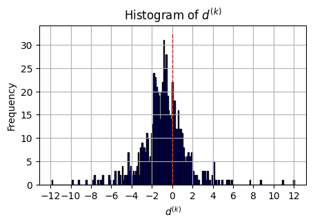
In Section 4, we introduced an SNR-weighted arbitrage regularization term in the loss function to enforce the arbitrage constraints. To evaluate the efficacy of this regularization, we compare a model trained with the complete loss $\mathcal{L}_{\text{total}}$ against a model trained on $\mathcal{L}_{\text{simple}}$, which does not include the arbitrage penalty term. As reported in Table 4, including the regularization term reduces all four statistics of the arbitrage penalties without compromising predictive accuracy, as measured by MAPE. By lowering both the mean and standard deviation, the regularization term shifts the arbitrage penalty distribution to the left and concentrates it more tightly around zero. This effect is more clearly illustrated in Figure 12, where the distribution of the regularized model (blue) exhibits a sharper, taller mode at zero. In contrast, the orange distribution shows wider distribution with the mean shifted to the right compared to the blue distribution mean. Furthermore, Figure 11 demonstrates that the model trained without the regularization term generates vol-surfaces with consistently higher arbitrage penalties with a peak around $0.1$. The regularization term mitigates the arbitrage penalties across the majority of the time series and suppresses the peak to $0.028$. Together, these results confirm that the SNR-weighted regularization term successfully minimizes arbitrage violations in the generated vol-surfaces.

Figure 11: Time-series comparison of arbitrage penalties of the generated vol-surfaces. The model trained without regularization term ($\mathcal{L}_{\text{simple}}$, orange) generated vol-surfaces with higher arbitrage penalty than the vol-surfaces from the model with SNR-weighted arbitrage penalty ($\mathcal{L}_{\text{total}}$, blue).

Figure 12: The distribution comparison of arbitrage penalties for generated vol-surfaces. The baseline model trained with $\mathcal{L}_{\text{simple}}$, shown in orange, exhibits a right-skewed penalty distribution, indicating more frequent arbitrage violations. The conditional diffusion model trained with $\mathcal{L}_{\text{total}}$, shown in blue, shifted the distribution toward zero.

Table 4: Summary statistics of the arbitrage between models. The mean of MAPE column shows the mean MAPE of the test set.

Model	Mean	Std	Min	Max	Mean of MAPE
With Arbitrage Penalty	0.003524	0.002645	0.000225	0.027898	3.0026
Without Arbitrage Penalty	0.012378	0.010938	0.000380	0.100377	3.0941

7 Conclusion

In this paper, we introduced a conditional Denoising Diffusion Probabilistic Model (DDPM) for forecasting one-day-ahead vol-surfaces. We demonstrated that the diffusion model provides an improved alternative to existing generative models when combined with the market conditioning set. We incorporated an explicit arbitrage penalty into the loss function that is dynamically weighted by the SNR, which suppresses arbitrage violations without destabilizing the training process. Our model not only achieved a lower overall MAPE than the benchmark generative model but also was shown to be better calibrated.

Appendix A Hyperparameters

Table A.1: Summary of Model Hyperparameters

Notation	Description	Value
$N_{\text{epochs}}$	Total number of training epochs	2000
$B$	Training batch size	64
$N$	Number of discrete diffusion timesteps	500
$\eta_{\text{min}}$	Minimum learning rate bound for plateau scheduler	1e-6
$\gamma_{\text{lr}}$	Learning rate decay factor	0.8
$P_{\text{lr}}$	Patience (consecutive epochs) for learning rate scheduler	300
$c_{\text{grad}}$	Maximum $L_{2}$-norm for gradient clipping	0.15
$\beta_{\text{EWMA}}$	Exponential moving average (EWMA) decay rate for network weights	0.995
$\alpha_{\text{short}}$	Short-term decay factor for historical vol-surfaces	0.3333
$\alpha_{\text{long}}$	Long-term decay factor for historical vol-surfaces	0.0952
$\alpha_{r}^{S}$	Short-term decay factor for underlying asset returns	0.156
$\alpha_{r}^{L}$	Long-term decay factor for underlying asset returns	0.118
$\alpha_{\sigma}^{S}$	Short-term decay factor for squared asset returns	0.3
$\alpha_{\sigma}^{L}$	Long-term decay factor for squared asset returns	0.15
$h_{m}$	Smoothing bandwidth across moneyness	0.002
$h_{\tau}$	Smoothing bandwidth across time-to-maturity (maturity)	0.1
$d_{\text{emb}}$	Sinusoidal time embedding dimension ($d_{\text{emb}}\geq 2$)	24

Appendix B Full Performance Metrics for All Trained Models

Table B.1: Full comparison of performance metrics for all 10 trained VolGAN models and the proposed Diffusion model (Part 1 of 2). VolGAN 3 was selected as the benchmark for comparison in the main text due to having the lowest Overall MAPE.

	ATM				OTM				ITM
Metric	1-Day	1-Week	1-Month	3-Month	1-Day	1-Week	1-Month	3-Month	1-Day	1-Week	1-Month	3-Month	Overall
VolGAN 1
MAPE (%)	5.4848	5.4079	5.2264	6.6949	7.3509	7.3813	7.9716	6.0041	3.1493	3.1892	3.0474	3.7308	4.6804
Std. of APE (%)	4.3854	4.8749	4.1418	4.7774	5.4913	5.3441	5.2115	4.0811	2.7181	2.7836	2.4780	2.5913
Mean CI Width	0.0069	0.0074	0.0070	0.0078	0.0105	0.0118	0.0112	0.0091	0.0061	0.0051	0.0055	0.0040
Std. CI Width	0.0020	0.0021	0.0017	0.0018	0.0018	0.0017	0.0016	0.0016	0.0013	0.0011	0.0012	0.0008
CI Breach %	71.8795	75.5140	82.2095	83.5007	74.7489	73.1707	77.7618	74.6055	84.2181	86.0832	84.7920	92.1091
VolGAN 2
MAPE (%)	4.9045	4.8584	4.7725	4.2313	5.7716	6.5407	5.7373	3.4782	3.1053	3.0444	3.0586	2.5059	4.1946
Std. of APE (%)	4.1963	4.1376	4.0179	3.6930	4.1804	4.7538	4.2727	2.4844	2.7093	2.7118	2.6850	2.3113
Mean CI Width	0.0355	0.0385	0.0326	0.0295	0.0488	0.0428	0.0388	0.0271	0.0516	0.0505	0.0528	0.0411
Std. CI Width	0.0209	0.0208	0.0200	0.0192	0.0167	0.0163	0.0154	0.0110	0.0262	0.0247	0.0247	0.0203
CI Breach %	16.2124	16.3558	15.6385	15.4950	12.6255	12.6255	10.7604	0.4692	19.0818	18.9383	17.5036	17.0732
VolGAN 3
MAPE (%)	4.8328	4.8300	4.6116	4.1195	4.8211	4.7215	4.6733	4.1599	2.9795	2.8638	2.9443	2.7594	3.8418
Std. of APE (%)	4.3189	4.1943	4.2765	3.7869	3.6335	3.5588	3.5381	3.0668	2.4808	2.4147	2.4355	2.2660
Mean CI Width	0.0263	0.0268	0.0244	0.0223	0.0424	0.0418	0.0389	0.0277	0.0197	0.0222	0.0178	0.0144
Std. CI Width	0.0101	0.0103	0.0097	0.0087	0.0171	0.0171	0.0159	0.0112	0.0065	0.0066	0.0066	0.0076
CI Breach %	22.9885	22.7011	26.1494	25.7184	13.7931	12.7874	13.9368	20.8333	51.7241	46.6954	54.1667	62.2126
VolGAN 4
MAPE (%)	5.1090	5.0465	4.9615	4.5056	3.4758	9.6190	9.9897	9.3729	3.1169	3.0795	3.2810	2.6945	4.8997
Std. of APE (%)	4.5452	4.3856	4.3040	4.0932	5.5650	5.8262	5.4114	4.5096	2.6147	2.5816	2.5417	2.2061
Mean CI Width	0.0248	0.0249	0.0235	0.0242	0.0292	0.0266	0.0284	0.0224	0.0387	0.0345	0.0330	0.0307
Std. CI Width	0.0055	0.0056	0.0057	0.0062	0.0119	0.0112	0.0121	0.0103	0.0040	0.0035	0.0032	0.0030
CI Breach %	26.5423	25.9685	28.2639	24.3902	58.6586	55.0933	62.2669	73.1707	22.0947	20.5165	27.1162	24.1033
VolGAN 5
MAPE (%)	5.8201	5.7422	5.6428	5.0018	7.0458	6.8858	6.5098	4.9647	2.7388	2.6938	2.7529	2.3215	4.5160
Std. of APE (%)	4.4566	4.3180	4.3644	3.8236	4.6511	4.8184	4.4095	3.4965	2.4420	2.4070	2.4130	2.1106
Mean CI Width	0.0229	0.0225	0.0236	0.0245	0.0639	0.0529	0.0482	0.0365	0.0374	0.0372	0.0347	0.0297
Std. CI Width	0.0128	0.0126	0.0128	0.0121	0.0240	0.0238	0.0200	0.0149	0.0149	0.0146	0.0134	0.0112
CI Breach %	52.0803	51.0760	50.2152	45.7675	13.7733	18.8235	16.2124	14.3472	25.5380	25.6815	28.5509	25.2511

Table B.2: Full comparison of performance metrics for all 10 trained VolGAN models and the proposed Diffusion model (Part 2 of 2).

	ATM				OTM				ITM
Metric	1-Day	1-Week	1-Month	3-Month	1-Day	1-Week	1-Month	3-Month	1-Day	1-Week	1-Month	3-Month	Overall
VolGAN 6
MAPE (%)	4.9009	4.8532	4.7405	4.1738	5.0297	5.8872	5.4906	4.3717	2.7423	2.6738	3.3214	4.1283	4.2254
Std. of APE (%)	4.3810	4.2428	4.2006	3.7055	4.5995	4.4943	4.1858	3.2465	2.3548	2.3079	2.6845	2.7560
Mean CI Width	0.0148	0.0143	0.0148	0.0139	0.0365	0.0355	0.0331	0.0236	0.0290	0.0292	0.0250	0.0240
Std. CI Width	0.0076	0.0073	0.0080	0.0072	0.0210	0.0191	0.0196	0.0129	0.0086	0.0085	0.0077	0.0069
CI Breach %	48.6413	51.3630	49.0674	46.9154	34.5768	34.4333	31.9943	39.1679	26.3989	24.9641	42.6112	61.4060
VolGAN 7
MAPE (%)	4.7346	4.6830	4.5588	4.1578	4.5364	4.4698	4.2965	3.5937	2.5437	2.5627	2.9411	3.4803	3.8615
Std. of APE (%)	4.1708	4.2017	4.0521	3.7747	3.5830	3.5084	3.3572	3.2544	2.4621	2.5217	2.8368	2.8927
Mean CI Width	0.0154	0.0145	0.0144	0.0097	0.0328	0.0323	0.0282	0.0185	0.0400	0.0383	0.0431	0.0287
Std. CI Width	0.0044	0.0043	0.0043	0.0057	0.0104	0.0102	0.0106	0.0072	0.0054	0.0053	0.0065	0.0045
CI Breach %	44.6198	47.0588	46.4849	56.9584	14.0603	12.7690	15.0646	39.1679	12.9125	13.6298	14.5841	38.8809
VolGAN 8
MAPE (%)	6.1914	5.9409	5.6571	5.3297	5.8692	6.9996	7.2199	6.4400	3.9085	3.9522	3.6069	3.1119	4.4841
Std. of APE (%)	4.9130	4.8142	4.5157	4.1559	4.7578	4.7563	4.7586	4.4847	2.9786	3.0048	2.9723	2.5855
Mean CI Width	0.0121	0.0121	0.0103	0.0100	0.0615	0.0604	0.0571	0.0422	0.0256	0.0259	0.0259	0.0236
Std. CI Width	0.0038	0.0039	0.0028	0.0026	0.0368	0.0361	0.0334	0.0244	0.0068	0.0072	0.0072	0.0058
CI Breach %	64.5624	64.7059	68.7231	70.0143	19.6556	20.6599	26.2554	34.5768	47.7762	49.3544	45.1937	41.4634
VolGAN 9
MAPE (%)	5.1526	5.2093	5.3758	8.9616	12.0051	11.9373	11.1095	4.8830	22.6214	22.4364	14.8209	12.6213	9.0688
Std. of APE (%)	4.2558	4.2584	4.2575	5.9750	5.1833	5.0434	4.6224	3.5354	9.2836	9.3468	6.7452	7.1482
Mean CI Width	0.0008	0.0008	0.0011	0.0011	0.0042	0.0040	0.0038	0.0029	0.0066	0.0068	0.0058	0.0065
Std. CI Width	0.0002	0.0002	0.0003	0.0003	0.0007	0.0007	0.0007	0.0005	0.0011	0.0012	0.0010	0.0012
CI Breach %	97.7045	96.9871	95.2654	98.5653	98.7088	98.7088	98.8522	88.9526	100.0000	100.0000	98.2783	98.7088
VolGAN 10
MAPE (%)	4.8474	4.8295	4.6663	4.2226	7.7716	7.5443	6.7917	4.2674	3.2081	3.1988	3.0942	2.4420	4.1273
Std. of APE (%)	4.2239	4.1958	4.0956	3.7226	4.9421	4.8144	4.3522	3.1403	2.5716	2.5842	2.5012	2.0886
Mean CI Width	0.0122	0.0125	0.0116	0.0088	0.0312	0.0301	0.0264	0.0153	0.0194	0.0188	0.0166	0.0107
Std. CI Width	0.0053	0.0056	0.0059	0.0036	0.0169	0.0163	0.0138	0.0059	0.0119	0.0108	0.0085	0.0037
CI Breach %	59.8277	59.8346	62.5538	66.5710	26.1206	27.5466	25.1076	55.9540	57.6753	58.8235	60.2582	63.5581
Diffusion
MAPE (%)	4.6907	4.6884	4.5146	4.0202	3.5264	3.4573	3.1542	2.4555	2.5129	2.4992	2.4184	2.2024	3.0026
Std. of APE (%)	4.0338	4.0091	3.8795	3.4909	2.6588	2.5785	2.3190	1.8739	2.3984	2.3844	2.2909	2.0393
Mean CI Width	0.0372	0.0369	0.0357	0.0327	0.0468	0.0457	0.0412	0.0311	0.0472	0.0463	0.0438	0.0384
Std. CI Width	0.0160	0.0159	0.0152	0.0134	0.0098	0.0095	0.0082	0.0057	0.0139	0.0137	0.0132	0.0124
CI Breach %	10.9195	10.4885	11.0632	10.0575	0.5747	0.7184	0.5747	1.0057	7.9023	7.9023	8.4770	7.9023