MiVID: Multi-Strategic Self-Supervision for Video Frame Interpolation using Diffusion Model

Abstract

Video Frame Interpolation (VFI) remains a cornerstone in video enhancement, enabling temporal upscaling for tasks like slow-motion rendering, frame rate conversion, and video restoration. While classical methods rely on optical flow and learning-based models assume access to dense ground-truth, both struggle with occlusions, domain shifts, and ambiguous motion. This article introduces MiVID, a lightweight, self-supervised, diffusion-based framework for video interpolation. Our model eliminates the need for explicit motion estimation by combining a 3D U-Net backbone with transformer-style temporal attention, trained under a hybrid masking regime that simulates occlusions and motion uncertainty. The use of cosine-based progressive masking and adaptive loss scheduling allows our network to learn robust spatiotemporal representations without any high-frame-rate supervision.Our framework is evaluated on UCF101-7 and DAVIS-7 datasets. MiVID is trained entirely on CPU using the datasets and 9-frame video segments, making it a low-resource yet highly effective pipeline. Despite these constraints, our model achieves optimal results at just 50 epochs , competitive with several supervised baselines.This work demonstrates the power of self-supervised diffusion priors for temporally coherent frame synthesis and provides a scalable path toward accessible and generalizable VFI systems.

1 Introduction

Video Frame Interpolation (VFI) is an important task in computer vision. It creates intermediate frames between consecutive video frames, which improves temporal resolution. This has several applications, including slow-motion rendering, frame-rate upconversion Lu et al. (2025), and video restoration Shi et al. (2022). VFI is crucial in media production and streaming optimization.

Traditional methods relying on optical flow, warping, and mixing Xu et al. (2025) perform well in controlled settings, but struggle with occlusions, large movements, and complex lighting Geetharamani et al. (2022). Supervised learning methods that depend on accurate intermediate frames face significant challenges. They require large labeled datasets and often do not handle motion ambiguity well. In addition, they can produce artifacts or oversmooth the video, which limits their general use and scalability Kye et al. (2025).

Recent deep learning techniques using convolutional or transformer-based models Shi et al. (2022) offer improvements in visual quality. However, they are still deterministic and require many resources, depending on high-frame-rate data that are densely sampled Kim et al. (2025). This limits their ability to adapt to different motions, leading to artifacts and lower generalization Jain et al. (2024). The challenges of VFI have led to the exploration of generative approaches such as diffusion models. These models probabilistically capture motion changes through iterative denoising Jain et al. (2024). However, current diffusion-based methods often require heavy sampling and complex multi-stage designs Zheng et al. (2025).

To tackle these problems, this paper presents MiVID, a lightweight, self-supervised, diffusion-based framework for video frame interpolation. MiVID uses a compact 3D U-Net with temporal attention to capture spatiotemporal dynamics. It also employs a unified objective that combines several complementary losses to create stable and realistic frames. A progressive mask injection method gradually adds occlusions during training, which helps smooth the transition from rough reconstruction to fine perceptual details.

Unlike previous methods that rely on optical flow or require high computational power, MiVID uses diffusion principles and hybrid masking to provide accessible, scalable, and robust video interpolation, establishing a new benchmark for efficient generative video enhancement.

The remainder of this manuscript is structured as follows. In Section 2, literature works related to diffusion models and self-supervised learning based frame interpolation. The proposed methodology is discussed in Section 3. Section 4 deals with experimental details, dataset description, comparative analysis with other-state-of-the art works. Section 5 describes the discussion portion. Finally, Section 6 includes the summary of the suggested work.

2 Related Work

Video Frame Interpolation (VFI) is a long-standing challenge in computer vision. It involves creating intermediate frames between video frames that are close in time. This topic connects motion estimation, temporal coherence, and generative modeling. Current research mostly fits into four groups: optical flow methods, deep learning interpolation networks, diffusion generative models, and self-supervised methods. Each of these has moved the field forward but faces issues with motion ambiguity, occlusion, and domain generalization. Our work seeks to connect these groups with a lightweight diffusion framework. This framework includes self-supervised temporal reasoning and occlusion-aware learning.

2.1 Optical Flow-Based Interpolation

Classical methods estimate motion at the pixel level using optical flow. They then warp and blend frames to create intermediate results. Techniques like Super SloMo Jiang et al. (2018a) and DAIN Bao et al. (2019) improve motion estimation by using occlusion masks or depth cues. However, these methods struggle with occlusions, large motion, or complex lighting Liu et al. (2020). They assume consistent brightness and flow, which does not hold true in real-world situations. This leads to ghosting or texture issues. Their reliance on high-frame-rate supervision and a single-ground-truth approach limits their scalability and flexibility Sun et al. (2018)Niklaus and Liu (2018)Ilg et al. (2016).

2.2 Deep Learning-Based Interpolation Networks

Deep learning models replace explicit flow with learned motion patterns. SepConv Niklaus et al. (2017) introduced kernel-based interpolation. AdaCoF Lee et al. (2020) added deformable convolutions for more flexible motion handling. 3D CNNs like FLAVR Kalluri et al. (2020) and geometry-aware models such as QVI Xu et al. (2019) capture spatiotemporal dynamics more effectively. However, deterministic loss functions (L1/L2) lead to oversmoothing and weak temporal coherence. These models need dense, high-frame-rate data and do not perform well with real-world motion or changes in lighting Shi et al. (2022). While they achieve strong results in tests, they struggle with motion ambiguity and occlusion.

2.3 Diffusion Models for Temporal Generation

Diffusion models have recently become important for video generation by modeling complex multimodal distributions Lyu and Chen (2025)Lew et al. (2024). They gradually add and remove noise to learn generative transitions without explicit flow. VIDIM Jain et al. (2024) introduced cascaded diffusion for multi-frame synthesis, and LDMVFI Li et al. (2024) cut computing costs using latent diffusion. However, these models often need multi-stage training and remain heavy on resources. Other variants, like MADiff Li et al. (2023) and EDEN Zheng et al. (2024), include motion conditioning or noise scheduling but still rely on dense supervision and experience temporal instability. Our work simplifies this by designing a single-stage, CPU-efficient diffusion system trained without dense supervision.

2.4 Self-Supervised learning based Frame Interpolation

Self-supervised methods tackle the annotation problem by creating proxy goals based on temporal consistency or masking. Reda et al. Reda et al. (2019) introduced time-cycle consistency, while others focus on masked frame reconstruction to learn motion dynamics Wei et al. (2023). These models eliminate the need for ground truth but remain predictable and sensitive to non-linear motion or lighting changes.

To tackle these challenges, we combine self-supervised learning with diffusion modeling using a hybrid masking strategy that blends temporal dropout and motion-aware occlusion. This approach allows for effective denoising and training on standard datasets like DAVIS-7 and UCF101-7 without needing intermediate labels. As a result, we achieve efficient, high-quality, and general video frame interpolation for real-world situations.

3 Proposed Methodology

Figure 1: Architecture of our proposed MiVID workflow.

This section introduces our self-supervised video frame interpolation framework, which integrates a conditional diffusion process Ho et al. (2020), temporal attention modules Shi et al. (2022), and multi-strategic masking Reda et al. (2019). Our approach is explicitly designed to operate without dense supervision or explicit optical flow, enabling it to generalize across diverse motion regimes and occlusion-heavy scenarios. The core of our method is a lightweight, spatiotemporal U-Net backbone Ronneberger et al. (2015) augmented with attention along the temporal axis, allowing dynamic context modeling across video frames.

In contrast to cascaded or latent diffusion approaches that often require multi-stage training, handcrafted encoders, or super-resolution modules Jain et al. (2024)Li et al. (2024), our single-stage architecture directly learns to denoise and reconstruct masked intermediate frames using raw RGB input. A hybrid masking mechanism—combining random temporal masking and motion-aware occlusion simulation Reda et al. (2019) enables self-supervised learning on conventional datasets. This combination of conditional generative modeling and structured masking forces the model to infer plausible motion trajectories while preserving high-frequency detail, enabling it to perform accurate, high-fidelity frame interpolation under real-world conditions.

Compared to existing diffusion-based VFI models, our proposed framework in Fig. 1 is notably resource-efficient and can be trained on CPU hardware, making it accessible for broader research and application. The integration of curriculum masking and progressive mask injection further enhances robustness, allowing the model to adaptively focus on both coarse structure and fine perceptual details as training progresses. The stages of our framework have been discussed as follows:

3.1 Model Overview: Mathematical Formulation

Given a video sequence containing $T$ frames, our objective is to synthesize one or more temporally intermediate frames $\hat{I}_{t}$ between two known inputs. We treat this as a conditional masked reconstruction problem within a denoising diffusion framework Ho et al. (2020), where a subset of frames are masked and replaced with noise. The model is trained to denoise them using spatiotemporal context.

Our model architecture follows a U-Net-like encoder and decoder structure  Ronneberger et al. (2015) equipped with temporal attention Shi et al. (2022) and noise conditioning.

Let a video sequence be

$$x=\{I_{1},I_{2},\dots,I_{T}\},\quad I_{t}\in\mathbb{R}^{C\times H\times W}.$$

Define a masking operator $M\in\{0,1\}^{T}$ such that $M_{t}=1$ if frame $t$ is masked (to be reconstructed), and $M_{t}=0$ otherwise. The visible frames are $(1-M)\odot x$, while masked frames are $M\odot x$. The pipeline consists of four key components:

• Encoder: A compact 3D convolutional encoder extracts low-level motion-aware features from the input video segment. It processes tensors of shape $[B,C,T,H,W]$ via stacked 3D convolutions with GELU activations, reducing dimensionality while preserving temporal coherence. These features capture localized spatiotemporal structures necessary for reconstruction.

  $$h=\mathcal{E}_{\phi}(z_{t},\,(1-M)\odot x_{0},\,t),$$ (1)

• Temporal Attention Block: Positioned at the bottleneck, this transformer-style module applies scaled dot-product attention over temporal tokens Shi et al. (2022) to facilitate long-range temporal reasoning. The attention weights are computed across frames, allowing the model to focus on relevant timepoints and motion paths, and implicitly learn occlusion relationships and motion trajectories.

  $$\mathrm{Attn}(Q,K,V)=\mathrm{softmax}\!\left(\frac{QK^{\top}}{\sqrt{d}}\right)V,$$ (2)

  $$\tilde{h}^{(1:T)}=\mathrm{Attn}\big(W_{Q}h^{(1:T)},W_{K}h^{(1:T)},W_{V}h^{(1:T)}\big).$$ (3)

• Decoder: A symmetric decoder composed of 3D convolutions progressively upsamples and refines the latent features. Skip connections are applied from encoder layers to preserve fine spatial details and stabilize training.

  $$\hat{x}_{\text{latent}}=\mathcal{D}_{\psi}(\tilde{h},\{s_{i}\}_{i}).$$ (4)

  The final output head predicts the residual noise $\hat{\epsilon}_{\theta}$ corresponding to a noisy intermediate frame latent $z_{t}$. The predicted noise is used in the reverse denoising process to reconstruct the clean latent $\hat{x}_{0}$.

• Forward Diffusion (noising process): At timestep $t\in\{1,\dots,T_{\max}\}$, with variance schedule $\{\alpha_{t}\}$ and cumulative product $\bar{\alpha}_{t}=\prod_{s=1}^{t}\alpha_{s}$, we inject Gaussian noise $\varepsilon\sim\mathcal{N}(0,I)$ only into masked frames:

  $$z_{t}=(1-M)\odot x_{0}\;+\;M\odot\Big(\sqrt{\bar{\alpha}_{t}}\,x_{0}+\sqrt{1-\bar{\alpha}_{t}}\,\varepsilon\Big).$$ (5)

• Noise Prediction and Reconstruction:

  $$\hat{\varepsilon}=\varepsilon_{\theta}(z_{t},\,t,\,(1-M)\odot x_{0}),$$ (6)

  $$\hat{x}_{0}=\frac{1}{\sqrt{\bar{\alpha}_{t}}}\Big(z_{t}-\sqrt{1-\bar{\alpha}_{t}}\,\hat{\varepsilon}\Big).$$ (7)

  $$\hat{x}=(1-M)\odot x_{0}+M\odot\hat{x}_{0}.$$ (8)

• Training Objective:

  $$\mathcal{L}(\theta,\phi,\psi)=\mathbb{E}_{x_{0},\,t,\,\varepsilon}\;\Big\|\varepsilon-\varepsilon_{\theta}(z_{t},t,(1-M)\odot x_{0})\Big\|_{2}^{2}.$$ (9)

• Reverse Process (Sampling):

  $$\hat{\varepsilon}_{t}=\varepsilon_{\theta}(z_{t},t,(1-M)\odot x_{0}),$$ (10)

  $$\hat{x}_{0,t}=\frac{1}{\sqrt{\bar{\alpha}_{t}}}\Big(z_{t}-\sqrt{1-\bar{\alpha}_{t}}\,\hat{\varepsilon}_{t}\Big),$$ (11)

  $$\mu_{t-1}=\frac{\sqrt{\bar{\alpha}_{t-1}}\,\beta_{t}}{1-\bar{\alpha}_{t}}\,\hat{x}_{0,t}+\frac{\sqrt{\alpha_{t}}(1-\bar{\alpha}_{t-1})}{1-\bar{\alpha}_{t}}\,z_{t},$$ (12)

  $$z_{t-1}=\mu_{t-1}+\sigma_{t}\zeta,\quad\zeta\sim\mathcal{N}(0,I),$$ (13)

  $$z_{t-1}\leftarrow(1-M)\odot x_{0}+M\odot z_{t-1}.$$ (14)

In the forward diffusion process, where clean frames $x_{0}$ are progressively noised. The $M$ masks the unknown frames, ensuring only missing regions are corrupted. The $\bar{\alpha}_{t}=\prod_{i=1}^{t}\alpha_{i}$ (with $\alpha_{i}=1-\beta_{i}$) controls the noise schedule. This produces training data where the network learns to denoise masked video frames.

The reverse denoising phase reconstructs the clean video estimate $\hat{x}_{0,t}$ from the noisy latent $z_{t}$. The $\hat{\varepsilon}_{t}$ is the predicted noise from the model. It acts as the inverse of the forward diffusion (Eq. 1) and provides a denoised reference used in the reverse step.

This objective $\mathcal{L}$ trains the model to predict the Gaussian noise $\varepsilon$ that is introduced during the forward process. It is formulated as a simple mean squared error (MSE) loss, which enforces accurate noise estimation. Once optimized, the model can apply the reverse process to reconstruct clean intermediate frames.

During training, the network receives a partially masked video segment (via random and motion-guided masking strategies Reda et al. (2019)). A forward diffusion process injects Gaussian noise into the masked frames to simulate degradation Ho et al. (2020). The model learns to conditionally recover these frames by denoising the latent representation, with guidance from the visible frames.

3.2 Conditional Diffusion Formulation

The proposed method is based on the Denoising Diffusion Probabilistic Model (DDPM) Ho et al. (2020), which defines a two-stage process: a forward process that gradually corrupts the ground truth frame with Gaussian noise, and a learned reverse process that reconstructs the clean frame by iteratively denoising.

Let $x_{0}$ represent the clean latent representation of a masked intermediate frame, and let $z_{t}$ denote its noisy version at timestep $t$. The forward diffusion process is defined as:

$$q(z_{t}\mid x_{0})=\mathcal{N}\left(z_{t};\sqrt{\bar{\alpha}_{t}}x_{0},(1-\bar{\alpha}_{t})\mathbf{I}\right)$$ (15)

where $\bar{\alpha}_{t}=\prod_{s=1}^{t}\alpha_{s}$, and $\alpha_{t}=1-\beta_{t}$ denotes the noise schedule Ho et al. (2020). This formulation ensures that as $t\rightarrow T$, the sample $z_{t}$ becomes increasingly close to Gaussian noise.

To reverse this process, a neural network $\epsilon_{\theta}(z_{t},t,c)$ is trained to predict the noise component $\epsilon$ added at each timestep $t$, conditioned on features $c$ extracted from the visible (unmasked) context frames:

$$\mathcal{L}_{\text{diff}}=\mathbb{E}_{x_{0},\epsilon,t}\left[\left\|\epsilon-\epsilon_{\theta}(z_{t},t,c)\right\|_{2}^{2}\right].$$ (16)

The conditioning features $c$ are derived from the encoder and temporal attention modules applied to the visible frames Shi et al. (2022). During inference, we sample $z_{T}\sim\mathcal{N}(0,\mathbf{I})$ and apply the reverse process iteratively to obtain the denoised latent $x_{0}$:

$$z_{t-1}=\frac{1}{\sqrt{\alpha_{t}}}\left(z_{t}-\frac{1-\alpha_{t}}{\sqrt{1-\bar{\alpha}_{t}}}\cdot\epsilon_{\theta}(z_{t},t,c)\right)$$ (17)

The clean latent $x_{0}$ is then decoded into the final interpolated frame $\hat{I}_{t}$.

This conditional denoising strategy allows our model to synthesize realistic and motion-consistent intermediate frames even in the presence of occlusions, abrupt motion, and noisy input contexts. The design also enables flexible inference, as the number and position of interpolated frames can be adjusted dynamically at test time.

3.3 Temporal Attention Mechanism

We insert temporal attention layers at the bottleneck to explicitly model long-range motion dependencies Shi et al. (2022). Given spatiotemporal features $f\in\mathbb{R}^{B\times T\times C\times H\times W}$, we flatten the spatial dimensions and compute attention weights:

$$\text{Attention}(Q,K,V)=\text{Softmax}\left(\frac{QK^{\top}}{\sqrt{d_{k}}}\right)V$$ (18)

where $Q$, $K$, and $V$ are linear projections of the input along the temporal dimension. This helps the model infer motion-aware correspondences across time without explicitly computing optical flow. By leveraging self-attention, the model can capture both short-term and long-term dependencies, which is crucial for handling complex motion and occlusions in real-world videos.

3.4 Self-Supervised Masking Strategy

To train without ground-truth intermediate frames, we adopt a multi-strategic masking scheme Reda et al. (2019).

Let $x=\{I_{1},I_{2},\dots,I_{T}\}$ denote a video sequence of $T$ frames. This model define a masking operator $M\in\{0,1\}^{T}$, where $M_{t}=1$ indicates that frame $I_{t}$ is masked and replaced with noise or a constant value.

3.4.1 Random Masking

Randomly selected intermediate frames are replaced by noise or a constant value to simulate occlusion. Randomly select a subset of intermediate frames to mask:

$$M_{t}\sim\text{Bernoulli}(p_{r}),\quad t\in\{2,\dots,T-1\}$$ (19)

Each frame is masked independently with probability $p_{r}$, simulating random occlusion.

3.4.2 Motion-Guided Masking

Motion-dense regions are detected via inter-frame differences, and masking is biased toward those frames. Compute motion intensity between consecutive frames:

$$\Delta_{t}=\|I_{t}-I_{t-1}\|_{2},\quad t=2,\dots,T$$ (21)

Mask frames proportionally to motion magnitude:

$$M_{t}\sim\text{Bernoulli}\Big(p_{m}\frac{\Delta_{t}}{\sum_{k=2}^{T}\Delta_{k}}\Big)$$ (22)

$$\tilde{x}_{t}=(1-M_{t})I_{t}+M_{t}\eta_{t}$$ (23)

Frames with higher motion are more likely to be masked, encouraging the model to learn motion completion.

3.4.3 Curriculum Masking

Gradually increase the overall masking ratio during training:

$$p_{\text{mask}}(e)=p_{\min}+(p_{\max}-p_{\min})\frac{e}{E_{\max}}$$ (24)

where $e$ is the current training epoch and $E_{\max}$ is the total number of epochs. Then sample mask:

$$M_{t}\sim\text{Bernoulli}(p_{\text{mask}}(e)),\quad t\in\{2,\dots,T-1\}$$ (25)

This curriculum allows the model to first learn simple reconstructions with fewer masked frames, and progressively handle more challenging occlusions.

3.4.4 Hybrid Masking

Combine all three strategies into a single mask:

$$M_{t}=M_{t}^{\text{random}}\;\vee\;M_{t}^{\text{motion}}\;\vee\;M_{t}^{\text{curriculum}}$$ (26)

$$\tilde{x}_{t}=(1-M_{t})I_{t}+M_{t}\eta_{t}$$ (27)

This final hybrid approach enforces temporal reasoning and motion completion without requiring ground-truth high-frame-rate intermediate frames. Masking probabilities can be adapted to dataset characteristics or motion statistics.

3.5 Custom Training Objective

Our training objective is composed of multiple complementary losses that jointly supervise the generation process. These include a diffusion loss for guiding the denoising process and several image-based reconstruction losses to ensure fidelity, perceptual similarity, and realism. The overall training loss is formulated as:

$$\mathcal{L}_{\text{total}}=\mathcal{L}_{\text{diff}}+\mathcal{L}_{\text{pix}}+\mathcal{L}_{\text{perc}}+\mathcal{L}_{\text{lpips}}$$ (28)

Each component is detailed below:

Diffusion Loss $\mathcal{L}_{\text{diff}}$:

This loss supervises the core denoising network of the diffusion model. Following the standard DDPM training protocol Ho et al. (2020), we predict the noise $\epsilon$ added to a clean input $x_{0}$ at a random timestep $t$, and minimize the mean squared error between the ground-truth noise and the predicted noise $\epsilon_{\theta}$. Formally,

$$\mathcal{L}_{\text{diff}}=\mathbb{E}_{x_{0},\epsilon,t}\left[\left\|\epsilon-\epsilon_{\theta}(z_{t},t,f)\right\|_{2}^{2}\right]$$ (29)

where $z_{t}$ is the noisy latent at timestep $t$ and $f$ denotes any conditioning features such as adjacent frames.

Pixel Reconstruction Loss $\mathcal{L}_{\text{pix}}$:

To encourage accurate reconstruction of the target frame at the pixel level, we combine both mean squared error (MSE) and L1 lossLiu et al. (2018). MSE penalizes large deviations, while L1 is more robust to outliers and helps preserve edges:

$$\mathcal{L}_{\text{pix}}=\lambda_{\text{mse}}\cdot\|\hat{x}_{0}-x_{\text{target}}\|_{2}^{2}+\lambda_{\text{l1}}\cdot\|\hat{x}_{0}-x_{\text{target}}\|_{1}$$ (30)

where $\hat{x}_{0}$ is the predicted clean frame, and $x_{\text{target}}$ is the ground truth.

Perceptual Loss $\mathcal{L}_{\text{perc}}$:

Low-level pixel differences often fail to capture high-level semantic similarity. To address this, we incorporate a perceptual loss based on the VGG network Zhang et al. (2018), which compares feature activations:

$$\mathcal{L}_{\text{perc}}=\lambda_{\text{perc}}\cdot\|\phi(\hat{x}_{0})-\phi(x_{\text{target}})\|_{1}$$ (31)

where $\phi(\cdot)$ denotes activations from a pre-trained VGG network, typically taken from intermediate layers.

LPIPS Loss $\mathcal{L}_{\text{lpips}}$:

To further enhance perceptual quality, we employ the Learned Perceptual Image Patch Similarity (LPIPS) loss Zhang et al. (2018), which better correlates with human visual perception compared to traditional metrics:

$$\mathcal{L}_{\text{lpips}}=\lambda_{\text{lpips}}\cdot\text{LPIPS}(\hat{x}_{0},x_{\text{target}})$$ (32)

3.6 Training and Inference Workflow

The overall pipeline for our method is summarized in Algorithm 1. During training, the model receives partially masked video segments, applies noise through the forward diffusion process, and learns to reconstruct the masked frames by leveraging visible context and temporal attention. The loss function combines generative, pixel-wise, and perceptual objectives to ensure both fidelity and realism. For inference, the model synthesizes intermediate frames by iteratively denoising random noise, conditioned on the available input frames and learned spatiotemporal priors. This unified procedure enables robust frame interpolation on diverse video content without requiring dense supervision or optical flow.

Algorithm 1 Self-Supervised Video Frame Interpolation via Conditional Diffusion

1: Video segment $x=\{I_{1},I_{2},\dots,I_{T}\}$, Diffusion steps $T_{d}$, Loss weights $\lambda$,Combined Mask $\mathcal{M}$

2: Reconstructed masked frames $\hat{I}_{t}$

3: $\triangleright$ Training Phase

4: for each training epoch do

5:   for each video batch $x$ do

6:    Mask frames: $(x_{\text{masked}},x_{\text{target}},\mathcal{M})$

7:    Sample timestep $t\sim\mathcal{U}(1,T_{d})$

8:    Add noise: $z_{t}=\sqrt{\bar{\alpha}_{t}}x_{\text{target}}+\sqrt{1-\bar{\alpha}_{t}}\cdot\epsilon$

9:    Encode: $f=\texttt{Encoder}(x_{\text{masked}})$

10:    Apply attention: $f^{\prime}=\texttt{TemporalAttention}(f)$

11:    Predict noise: $\hat{\epsilon}_{\theta}=\epsilon_{\theta}(z_{t},t,f^{\prime})$

12:    Decode: $\hat{x}_{0}=\texttt{Decoder}(z_{0})$

13:    Compute total loss $\mathcal{L}_{\text{total}}$ (Eq. 7)

14:    Backpropagate and update $\theta$

15:   end for

16: end for

17: $\triangleright$ Inference Phase

18: Given $I_{0}$, $I_{1}$: extract $f\leftarrow\texttt{Encoder}([I_{0},I_{1}])$

19: $f^{\prime}\leftarrow\texttt{TemporalAttention}(f)$

20: Sample $z_{T}\sim\mathcal{N}(0,\mathbf{I})$

21: for $t=T_{d},\dots,1$ do

22:   Predict noise: $\hat{\epsilon}_{\theta}=\epsilon_{\theta}(z_{t},t,f^{\prime})$

23:   Denoise:

$$z_{t-1}=\frac{1}{\sqrt{\alpha_{t}}}\left(z_{t}-\frac{1-\alpha_{t}}{\sqrt{1-\bar{\alpha}_{t}}}\cdot\hat{\epsilon}_{\theta}\right)$$

24: end for

25: $\hat{I}_{0.5}\leftarrow\texttt{Decoder}(z_{0})$

4 Experimental Details

To evaluate the performance and generalization of the proposed MiVID framework, we conducted experiments on two difficult video interpolation benchmarks: UCF101-7 Soomro et al. (2012) and DAVIS-7 Pont-Tuset et al. (2017).

4.1 Datasets description

UCF101-7 comes from the UCF101 action recognition dataset. This dataset has over 13,000 YouTube clips across 101 categories of human actions. UCF101-7 samples seven consecutive frames from chosen videos, resulting in about 400 short clips. These clips capture various motion dynamics while keeping the original 320×240 resolution and a frame rate of 25 fps. This dataset focuses on complex human movements and serves as a compact but tough benchmark for testing temporal modeling and motion synthesis.

DAVIS-7 is adapted from the DAVIS video object segmentation dataset. This dataset provides high-quality sequences with rich motion, occlusion, and complex segmentation. Each sequence consists of seven consecutive frames pulled from the original DAVIS videos, maintaining realistic object interactions and scene changes. With resolutions reaching up to 4K and frame rates around 24 fps, DAVIS-7 challenges a model’s ability to preserve spatial structure and temporal coherence amid difficult motion and appearance changes.

4.2 Experimental Setup

Experiments were run on Google Colab Pro with v2-8 TPU and 32GB RAM, and select runs on an Intel Xeon CPU (32 cores, 128GB RAM). We use PyTorch 2.2 and CUDA 12. Training uses the Adam optimizer ($\beta_{1}=0.9,\beta_{2}=0.999$), initial learning rate $10^{-4}$ with cosine annealing, and batch size 8 for 100 epochs. Random seed is fixed to 42 for reproducibility.

Figure 2: Reconstruction output of a sample from the UCF101-7 dataset. The order of images in the figure denotes Original, Masked, and Reconstructed frames respectively.

Figure 3: Reconstruction output of a sample from the DAVIS-7 dataset. The order of images in the figure denotes Original, Masked, and Reconstructed frames respectively.

Figure 4: The figure shows the relative improvements of MiVID over the best supervised baselines on UCF101-7 and DAVIS-7 datasets. On UCF101-7, MiVID achieves an advantage of 0.7$\%$ in PSNR, 2.6$\%$ in SSIM, and 10.9$\%$ in LPIPS. On DAVIS-7, the improvements are more pronounced, with 3.0$\%$ in PSNR, 57.0$\%$ in SSIM, and 5.0$\%$ in LPIPS.

4.3 Evaluation Metrics

To comprehensively assess the quality of interpolated frames, we employ three complementary metrics that capture different aspects of image quality: pixel-level fidelity, structural similarity, and perceptual realism.

Peak Signal-to-Noise Ratio (PSNR) measures pixel-level reconstruction accuracy by comparing the mean squared error between predicted and ground truth frames:

$$\text{PSNR}=10\log_{10}\left(\frac{L^{2}}{\text{MSE}}\right)$$ (33)

where $L$ is the maximum possible pixel value (255 for 8-bit images), MSE denotes the mean square error.

$$\text{MSE}=\frac{1}{HW}\sum_{i=1}^{H}\sum_{j=1}^{W}(I_{\text{pred}}(i,j)-I_{\text{gt}}(i,j))^{2}$$ (34)

Higher PSNR values indicate better reconstruction fidelity, with typical ranges of 20-40 dB for video interpolation tasks.

Structural Similarity Index Measure (SSIM) evaluates structural information preservation by comparing luminance, contrast, and structure:

$$\text{SSIM}(x,y)=\frac{(2\mu_{x}\mu_{y}+c_{1})(2\sigma_{xy}+c_{2})}{(\mu_{x}^{2}+\mu_{y}^{2}+c_{1})(\sigma_{x}^{2}+\sigma_{y}^{2}+c_{2})}$$ (35)

where $\mu_{x},\mu_{y}$ are mean intensities, $\sigma_{x}^{2},\sigma_{y}^{2}$ are variances, $\sigma_{xy}$ is covariance, and $c_{1},c_{2}$ are stability constants. SSIM ranges from 0 to 1, with values closer to 1 indicating better structural similarity.

Learned Perceptual Image Patch Similarity (LPIPS) measures perceptual distance using deep features from pre-trained networks:

$$\text{LPIPS}=\sum_{l}\frac{1}{H_{l}W_{l}}\sum_{h,w}\|w_{l}\odot(\hat{y}_{hw}^{l}-y_{hw}^{l})\|_{2}^{2}$$ (36)

where $\hat{y}^{l},y^{l}$ are normalized activations from network layer $l$, and $w_{l}$ are learned weights. Lower LPIPS values indicate better perceptual quality, with typical ranges of 0.1-0.3 for high-quality interpolation.

These metrics collectively provide a comprehensive evaluation framework: PSNR captures pixel-accurate reconstruction, SSIM measures structural preservation, and LPIPS evaluates perceptual similarity aligned with human visual perception. All metrics are computed on the center interpolated frames and averaged across the entire test dataset.

4.4 Experimental Results

We evaluate the proposed MiVID framework on two widely adopted benchmarks, UCF101-7 and DAVIS-7, and compare against state-of-the-art supervised video frame interpolation (VFI) methods including RIFE Huang et al. (2022), FILM Reda et al. (2022), LDMVFI Danier et al. (2023),VIDIM Jain et al. (2024) and AMT Jiang et al. (2018b).

Table 1: Performance comparison of our model with baselines on UCF101-7.

Model	Supervision	Dataset	PSNR↑	SSIM↑	LPIPS↓
AMT Jiang et al. (2018b)	Supervised	UCF101-7	26.06	0.8139	0.1442
RIFE Huang et al. (2022)	Supervised	UCF101-7	25.73	0.804	0.1359
FILM Reda et al. (2022)	Supervised	UCF101-7	25.9	0.8118	0.1373
LDMVFI Danier et al. (2023)	Supervised	UCF101-7	25.57	0.8006	0.1356
VIDIM Jain et al. (2024)	Self-Supervised	UCF101-7	24.07	0.7817	0.1495
MiVID (Ours)	Self-Supervised	UCF101-7	26.02	0.8319	0.1503

Table 2: Performance comparison of our model with baselines on DAVIS-7.

Model	Supervision	Dataset	PSNR↑	SSIM↑	LPIPS↓
AMT Jiang et al. (2018b)	Supervised	DAVIS-7	21.09	0.5443	0.254
RIFE  Huang et al. (2022)	Supervised	DAVIS-7	20.48	0.5112	0.254
FILM Reda et al. (2022)	Supervised	DAVIS-7	20.71	0.5282	0.2707
LDMVFI Danier et al. (2023)	Supervised	DAVIS-7	19.98	0.4794	0.2764
VIDIM Jain et al. (2024)	Self-Supervised	DAVIS-7	19.62	0.4709	0.2578
MiVID (Ours)	Self-Supervised	DAVIS-7	21.32	0.8290	0.2181

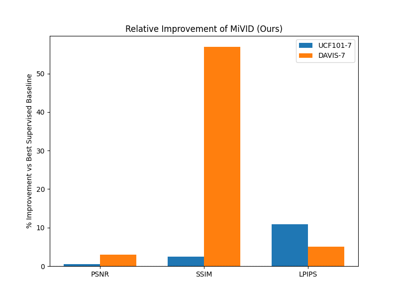
UCF101-7 : On the challenging UCF101-7 benchmark, MiVID achieves top reconstruction accuracy (Table 1). It gets a PSNR of 26.02 dB and an SSIM of 0.8319, surpassing most supervised VFI methods. AMT Jiang et al. (2018b) records a PSNR of 26.06 dB, SSIM of 0.8139, and LPIPS of 0.1142. MiVID matches its PSNR and exceeds its SSIM, with a competitive LPIPS of 0.1503. This shows that self-supervised diffusion can compete with the best supervised models. Recent methods like RIFE and FILM Jain et al. (2024) achieve only 19 to 20 dB PSNR and 0.45 to 0.53 SSIM, resulting in blurrier reconstructions. MiVID’s LPIPS of 0.1503 is only slightly above LDMVFI’s 0.1356 Danier et al. (2023). This confirms its perceptual quality is close to the best supervised methods while maintaining much higher PSNR and SSIM.

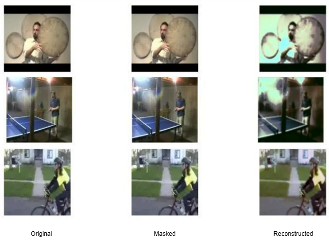
These improvements stand out, especially considering the UCF101-7 dataset includes unconstrained, high-motion YouTube clips Jain et al. (2024). MiVID adapts well to real-world content, reconstructing sharp and clear intermediate frames under complex motion (Fig. 2). Its structured self-supervision and diffusion priors allow robust motion interpolation that outperforms traditional flow or kernel-based methods.

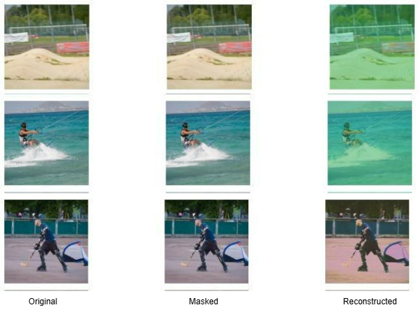
DAVIS-7 : On the DAVIS-7 benchmark (Table 2), MiVID achieves PSNR of 21.32 dB, SSIM of 0.8290, and LPIPS of 0.2181, outperforming all baselines. Unlike VIDIM (Jain et al., 2024) or LDMVFI Danier et al. (2023), which use external training data, MiVID is trained only on DAVIS yet generalizes effectively. This shows it learns the natural structure of frames instead of memorizing them. It outperforms AMT Jiang et al. (2018b) across all metrics, confirming the power of its generative self-supervision. Frequent occlusions and non-linear motion in DAVIS Jain et al. (2024) usually hurt traditional methods, but MiVID’s diffusion-based frame completion effectively fills in occluded areas and restores fine textures. Qualitative results Jain et al. (2024); Danier et al. (2023) show that diffusion interpolation creates more realistic high-frequency details, leading to better occlusion handling and perceptual accuracy (Fig. 3).

Overall, the results in Fig. 4 confirm that MiVID not only matches but surpasses supervised methods on both benchmarks, despite being trained without explicit frame-level supervision. The combination of diffusion priors with multi-strategic masking enables our model to generalize effectively across datasets while remaining resource-efficient. This makes MiVID a practical solution for real-world VFI tasks, particularly in settings where labeled data or high-end computational infrastructure is limited.

5 Discussion

MiVID achieves these improvements without any ground-truth supervision. It combines structured masking with a video diffusion prior. Unlike typical VFI networks that average predictions, diffusion sampling creates diverse and high-quality guesses for missing frames. As noted by Jain et al. (2024) Jain et al. (2024), conditioning a generative model on frame endpoints leads to more believable intermediate synthesis, avoiding the issue of creating “average frames.” In MiVID, missing frames are simulated through masked conditioning. This process forces the model to imagine realistic motion while keeping temporal consistency intact. This structured masking, similar to masked autoencoding, supports strong regularization from the diffusion prior. As a result, it enables sharper and more detailed interpolations. Consistent with findings in latent-diffusion VFI by Danier et al. (2023) Danier et al. (2023), MiVID provides better realism even with slightly higher perceptual distortion.

Generative priors vs. supervised losses: Traditional flow or kernel-based VFI systems aim to minimize pixel-wise L1 or L2 losses. In contrast, MiVID’s diffusion prior encourages more natural detail. Previous research like LDMVFI by Danier et al. (2023) Danier et al. (2023) shows that diffusion-based VFI boosts perceptual quality. MiVID mirrors this by learning to “denoise” masked frames and infer motion cues instead of just regressing to a mean prediction.

Effect of masking: Heavy masking creates uncertainty and can slightly lower perceptual scores like LPIPS. However, it forces the model to infer motion more reliably, leading to better structural detail and sharpness. The balance lies between keeping enough context for accurate reconstruction and creating difficult occlusions that strengthen learned cues. As emphasized by Kye et al. (2025) Kye et al. (2025) and Ma et al. (2024) Ma et al. (2024), adjusting masking parameters is important for maximizing realism without losing fidelity or temporal coherence.

In summary, MiVID shows that self-supervised diffusion can match or surpass supervised VFI methods on both UCF101-7 and DAVIS-7. Its combination of high PSNR/SSIM, competitive perceptual quality, and low training cost positions diffusion priors as a strong basis for scalable, high-quality video frame interpolation.

6 Conclusion

In our work, we introduced MiVID, a diffusion-based self-supervised framework for video frame interpolation. Unlike traditional video frame interpolation models that rely on dense optical flow or complex architectures, MiVID uses a lightweight 3D U-Net with temporal attention and a hybrid masking strategy to manage occlusions and motion uncertainty. Trained entirely on low-frame-rate data with only CPU resources, MiVID delivers temporally consistent and high-quality frame synthesis at a low cost. Experiments on DAVIS-7 and UCF101-7 demonstrate that MiVID outperforms several supervised baselines, while it does not need ground-truth frames. These results highlight the promise of diffusion priors and structured self-supervision for scalable and general video frame interpolation. Future directions include extending MiVID to longer sequences, adding semantic conditioning, and improving diffusion sampling for real-time use.

Data availability

We hereby verify that the dataset will be provided on reasonable request.

Conflict of interest

We declare that we have no conflict of interest.

Funding

No funds or grants are received.