Discovering causal relationships between time series with spatial structure

Abstract

Causal discovery is the subfield of causal inference concerned with estimating the structure of cause-and-effect relationships in a system of interrelated variables, as opposed to quantifying the strength or describing the form of causal effects. As interest in causal discovery builds in fields such as ecology, public health, and environmental sciences where data is regularly collected with spatial and temporal structures, approaches must evolve to manage autocorrelation and complex confounding. As it stands, the few proposed causal discovery algorithms for spatiotemporal data require summarizing across locations, ignore spatial autocorrelation, and/or scale poorly to high dimensions [32, 16]. Here, we introduce a developing framework that extends time-series causal discovery to systems with spatial structure, building upon work on causal discovery across contexts and methods for handling spatial confounding in causal effect estimation [12, 28]. We close by outlining remaining gaps in the literature and directions for future research.

Keywords: latent spatial confounder, conditional independence, causal discovery

1 Introduction

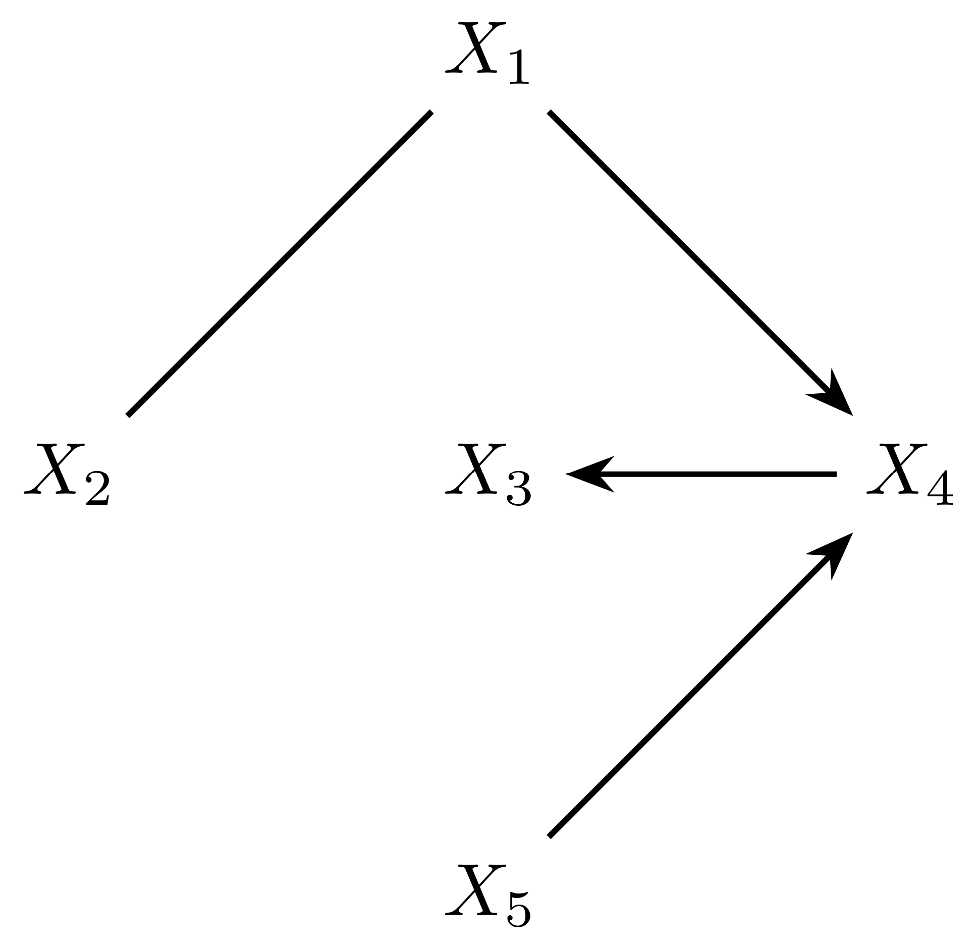
The identification of cause-and-effect relationships from observational data, also known as causal discovery, has always been at the center of scientific research [36]. In causal discovery, a system $\mathcal{X}$ of potentially interrelated variables of which we observe $\mathbf{X}=\{X_{1},...,X_{p}\}$ is analyzed to determine whether each pair of variables $X_{i},X_{j}\in\mathbf{X},i\neq j$ has a causal relationship whereby an intervention in/manipulation of $X_{i}$ leads to change in $X_{j}$. A causal discovery algorithm outputs an estimate of where (if any) causal relationships exist in the given system (e.g. fig. 1), providing key knowledge for causal model building, effect estimation, and/or counterfactual inference [36].

Statistical methods with this explicit goal have only emerged in the last three decades, however, and are still catching up to the complexity of practically available data [6, 14]. Spatiotemporal data pose particular difficulty for causal discovery methods due to autocorrelation between observations and with latent confounders that may mask or distort relationships [32]. In this short communication, we posit that existing causal discovery algorithms for independent and identically distributed time series can be adapted to time series with spatial structure by leveraging the theoretical results of causal discovery across contexts and latent spatial confounding in causal effect estimation [52, 28, 12].

In the following sections, we give an introduction to causal discovery and its underpinning conditional independence tests. We motivate the extension of causal discovery methods to spatiotemporal systems, and briefly review the state of the spatiotemporal causal discovery literature. We then discuss what causal discovery can learn from methods that address unobserved spatial confounding in causal effect estimation, and how this allows us to extend time series causal discovery to systems with spatial structure. We close by addressing the strengths and limitations of this extension and identifying promising areas of future research.

2 Causal discovery

The graphical causal approach proposes that systems can be represented by graphs in which causal variables are connected to their effects by directed edges (arrows) without forming feedback loops (fig. 1) [64, 35]. Causal graph structures are often defined by subject expert consensus or as a representation of a specific hypothesis [40, 31]. In either case, some confirmation bias may be present as only hypotheses previously considered in the literature and/or by the modeller can be put forth. There are also instances where no good hypotheses exist a priori to describe a system and exploratory analysis must be undertaken, motivating estimation of a causal graph from observational data.

Figure 1: An example of a causal graph estimated via constraint-based causal discovery for an observed system $\mathbf{X}=\{X_{1},X_{2},X_{3},X_{4},X_{5}\}$. An edge directed $X_{i}\rightarrow X_{j}$ indicates that $X_{i}$ causes $X_{j}$. An undirected edge $X_{i}\mathrel{\rule[2.15277pt]{6.99997pt}{0.4pt}}X_{j}$ indicates a causal connection where the direction is unresolvable (i.e. $X_{i}$ may cause $X_{j}$ or vice versa).

There are two principal approaches to causal discovery. Score-based causal discovery methods estimate a best-fit graph by minimizing a causally-relevant loss function across the space of possible graphs [5, 21]. Constraint-based methods iterate through all pairs of variables, testing their independence conditional on other variables in the system, and estimate cause-and-effect relationships by eliminating structures that are inconsistent with conditional independencies and/or do not meet assumptions [61, 36]. We focus on constraint-based methods here as they do not impose any inherent parametric or functional assumptions and thus maintain flexibility in the face of the complex spatiotemporal structures considered further in this paper [14, 6].

2.1 Constraint-based causal discovery

The PC (Peter-Clark) algorithm was proposed in 1991 as the first asymptotically correct constraint-based causal discovery algorithm that could handle more than a few independent and identically distributed variables [62]. In the decades since, the logic of the PC algorithm has been a popular jumping off point for extensions [45, 50, 16, 65, 53].

For PC and PC-derived algorithms, the goal is to estimate the placement and direction of edges in the causal graph of a system of variables. Given a system with $n$ i.i.d. observations of $p$ variables $\mathbf{X}=\{X_{1},...,X_{p}\}$, the algorithm first supposes a fully connected graph with undirected edges between all pairs $X_{i},X_{j}\in\mathbf{X},i\neq j$. It then searches for separating sets $\mathbf{A}_{ij}\subseteq\mathbf{X}\setminus\{X_{i},X_{j}\}$ such that $X_{i}\mathrel{\perp\!\!\!\perp}X_{j}\mathrel{\,|\,}\mathbf{A}_{ij}$. Where (conditional) independence is found, or, equivalently, when such a set $\mathbf{A}_{ij}$ exists, the variables $X_{i},X_{j}$ must not be causally connected and the edge between them is deleted.

Once the placement of edges has been determined, they are directed according to the following constraints. Where dependence between otherwise (conditionally) independent variables $X_{i}$ and $X_{j}$ is introduced by conditioning on a mutually adjacent variable $X_{k}$, a collider or common cause is indicated and edges are directed $X_{i}\rightarrow X_{k}\leftarrow X_{j}$. For example, $X_{1}\rightarrow X_{4}\leftarrow X_{5}$ in fig. 1 would be indicated by the relationships $X_{1}\mathrel{\perp\!\!\!\perp}X_{5};X_{1}\mathrel{\mathchoice{\mathrel{\hbox to0.0pt{\kern 6.38892pt\kern-5.27776pt$\displaystyle\not$\hss}{\mathrel{\perp\!\!\!\perp}}}}{\mathrel{\hbox to0.0pt{\kern 6.38892pt\kern-5.27776pt$\textstyle\not$\hss}{\mathrel{\perp\!\!\!\perp}}}}{\mathrel{\hbox to0.0pt{\kern 2.75006pt\kern-4.45831pt$\scriptstyle\not$\hss}{\mathrel{\perp\!\!\!\perp}}}}{\mathrel{\hbox to0.0pt{\kern 1.25006pt\kern-3.95834pt$\scriptscriptstyle\not$\hss}{\mathrel{\perp\!\!\!\perp}}}}}X_{5}\mathrel{\,|\,}X_{4}$. Once colliders have been determined, remaining undirected edges are directed as possible to avoid inducing feedback loops/cycles and so as not to create false colliders. Edges may remain undirected when direction is not resolvable according to the constraints, such as $X_{2}\mathrel{\rule[2.15277pt]{6.99997pt}{0.4pt}}X_{1}$ in fig. 1 [36].

The PC algorithm makes the following assumptions [62, 36]:

• Faithfulness (also known as the causal Markov condition): Conditional independence relationships faithfully correspond to causal structures;

• Sufficiency: All relevant variables are observed;

• Stability: Relationships are consistent across observations.

Various extensions relax the faithfulness [45], sufficiency [65], and/or stability [16, 53] assumptions.

2.2 Conditional independence testing

The rigor of constraint-based causal discovery hinges on consistent, accurate conditional independence testing in addition to its assumptions. Algorithms tend to be independence test-agnostic, however, and rarely enforce the use of any particular test or make claims of asymptotic correctness beyond the “oracle” setting where independence tests make no errors [50, 39, 14, 6].

Algorithms avoid committing to any particular conditional independence test partially because none are particularly good. Shah & Peters proved in 2020 that there is no nontrivial test that can distinguish between the null and alternative hypotheses of conditional independence and dependence with consistent power greater than the significance level [58]. Restrictions must be placed on the null to ensure power at any alternative.

[58] propose the generalized covariance measure, or GCM, as a practical approach to testing conditional independence. The null hypothesis of this test is that $X_{i}$ and $X_{j}$ are independent given $\mathbf{A}$:

$$\begin{split}\text{H}_{0}:\,&X_{i}\mathrel{\perp\!\!\!\perp}X_{j}\mathrel{\,|\,}\mathbf{A},\,\text{or, equivalently, }\\ &\,\mathbb{P}(X_{i},X_{j}\mathrel{\,|\,}\mathbf{A})=\mathbb{P}(X_{i}\mathrel{\,|\,}\mathbf{A})\mathbb{P}(X_{j}\mathrel{\,|\,}\mathbf{A}).\end{split}$$

The GCM test approximates the conditional distributions $\mathbb{P}(X_{i}\mathrel{\,|\,}\mathbf{A})$ and $\mathbb{P}(X_{j}\mathrel{\,|\,}\mathbf{A})$ with functions $\hat{f}$ and $\hat{g}$ estimated by regressing $X_{i}$ on $\mathbf{A}$ and $X_{j}$ on $\mathbf{A}$, respectively. A normalized sum similar to partial correlation of the product of residuals from fitted $\hat{f}$ and $\hat{g}$ is calculated. If the absolute value of this statistic is significantly large, the null hypothesis of independence is rejected. See section 5.1.1 for further discussion of significance thresholds.

No one function or model class is proposed to be ideal for the GCM test; any model with a sufficiently low out-of-sample mean squared prediction error and which meets smoothness criteria for all distributions in the null space can be used. Shah and Peters (2020) use kernel ridge regression in examples; see [58] for proofs, empirical support, and further model requirement details. [56] use generalized additive models and boosted regression trees in their extension of the GCM test to nonlinear dependence. We discuss practical aspects of model selection in light of spatiotemporal causal discovery in section 4.

3 Causal discovery for spatiotemporal data

Methods for causal discovery and conditional independence testing described so far assume all variables are independent and identically distributed, and that there are no confounding variables missing from the system. Data distributed across space and time are often autocorrelated, however, and may depend on unobserved time-lagged and spatial confounders [11, 12]. These obstacles can be dealt with differently according to the goal or overarching question asked of causal discovery.

Much literature on causal discovery for spatiotemporal data currently focuses on estimating patterns of influence within and/or between a handful of variables on a large spatiotemporal scale [68, 60, 59, 23, 29]. Spatial autocorrelation is often ignored according to domain knowledge [60, 59] or removed by estimating effectively independent spatial factors that aggregate nearby points [68, 23, 33, 51, 63]. While some methods allow for relationships to vary continuously with time [25], others look at temporal snapshots [29]. The estimated causal patterns summarize observed phenomena and can inform extrapolative forecasting models (fig. 2A).

Because latent pattern methods usually focus on changes across space and time for a single variable, latent confounders are often not explicitly addressed, only considered temporally, or assumed exogenous [29, 44].

A relatively understudied goal of causal discovery for spatiotemporal data is to infer the underlying structures of causal relationships between variables whose observations are distributed and autocorrelated across space and time. This approach imagines that there are latent mechanistic relationships that vary from an underlying central truth across space and/or time. These “latent mechanism,” rather than “latent pattern,” methods are more relevant for fields like ecology, economics, and public health, where interpretability of causal discovery output has policy and management implications (see illustration in fig. 2B; [41]).

Figure 2: Simplified, hypothetical illustrations of systems for which spatiotemporal (A) latent pattern or (B) latent mechanism causal discovery is relevant. A. In this system, arrows show how air pollutants from a volcano eruption causally spread across the world. Modified from [29]. B. In this system, fires cause instantaneous changes in forest cover across Great Britain, which in turn causes changes in a theoretical species’ abundance at a time lag. Although the variables are spatially distributed, practitioners seeking to understand causes of an observed shift in species abundance will be more interested in the mechanisms of change between variables than the spatiotemporal patterns of each variable.

This paper seeks to address spatiotemporal autocorrelation and confounding relevant to latent mechanism causal discovery, which has yet to receive much attention [6, 32]. The framework for spatiotemporal latent mechanism causal discovery we outline in the following sections provides researchers and decision makers ways to empirically derive causal models from complex spatiotemporal data and communicate accessibly.

3.1 Time series causal discovery

Temporal structures necessitate a treatment of autocorrelation and lagged effects. Autocorrelation can arise when values of a variable at one time are caused by values of that variable in the past [18]. By shifting whole time series back by some time lag and including the shifted variables as other points, or nodes, in the system, we can explicitly test for autocorrelated relationships [49]. These shifted time series also allow us to test for relationships between different variables that act at a time lag and would be confounded or at least over-simplified in non-temporal causal discovery [3].

The maximum time lag to consider must be chosen by the researcher as a hyperparameter [50, 39]. The choice is a tradeoff between potentially oversimplifying mechanistic processes if maximum lag is too low, or unnecessarily complicating the system and reducing power if too high, as shifting increases the number of nodes from $p$ observed time series to $p+Tp$, where $T$ is the maximum time lag considered.

Despite this increase in the number of nodes and tests, causal discovery for time series are not much more complex than methods for i.i.d. data since we assume effects never precede their causes. Time-series extensions of constraint-based causal discovery are thus focused on how to reduce complexity by best taking advantage of temporal structures [1].

The PCMCI+ algorithm is an example of a popular constraint-based, PC-derived method to efficiently discover time-lagged and instantaneous relationships between time series [52]. It optimizes the PC algorithm for time series by splitting the task of causal discovery into two stages: one for lagged effects, and another for instantaneous. The lagged stage mirrors the PC algorithm, considering only edges between nodes in the “present” ($\mathbf{X}_{t}$) and “past” ($\mathbf{X}_{t-\tau},1\leq\tau\leq T$). Since we assume effects cannot precede their causes, the directions of all edges discovered in the lagged phase are known and flow in the direction of time. It follows that no shared neighbor in the past can be a collider, or common effect, of two present nodes as that would imply an edge directed backwards in time. Furthermore, since only colliders can induce dependence, the inclusion by default of adjacent past nodes in separating sets $\mathbf{A}_{it,jt}\subseteq\mathbf{X}/\{X_{it},X_{jt}\}$ cannot falsely lead to failure to reject tests of $X_{it}\mathrel{\perp\!\!\!\perp}X_{jt}\mathrel{\,|\,}\mathbf{A}_{it,jt}$. When searching for separating sets between present nodes in the instantaneous phase, we can therefore restrict the search space to sets including past nodes adjacent to $X_{i,t}$ and/or $X_{j,t}$ without worrying about potential colliders.

Most assumptions of the PC algorithm are also made by PCMCI+; the time series algorithm assumes causal faithfulness, sufficiency, and stability of relationships across time [52]. Compared to other time series causal discovery algorithms, however, PCMCI+ avoids assumptions on the linearity and distribution of variables [39, 19], and is relatively unique in allowing both time-lagged and instantaneous relationships [50, 27, 1]. Relaxation of the causal sufficiency and stability assumptions have been developed, but at the cost of higher computational complexity and data requirements [24, 10, 53, 44, 11].

PCMCI+ assumes i.i.d. noise across the system given temporal autocorrelation and time-lagged relationships have been dealt with explicitly [52]. The algorithm has been shown to be highly sensitive to violations of this assumption when data have been collected with spatial structures, even if nodes are included as a pre-specified spatial grid [30]. To use the efficient logic of PCMCI+ for spatiotemporal latent mechanism causal discovery, we must draw upon methods for spatial causal inference and explicitly extend the algorithm.

3.2 Spatial causal discovery

In latent pattern causal discovery, nodes represent explicit spatial points, and a constraint similar to temporal information can be used to improve efficiency when one assumes causes do not “jump” over locations and must instead propagate through adjacent areas up to a maximum distance threshold [74, 29]. Latent mechanism causal discovery does not have to deal with the same explosion of complexity that comes with making each location its own node, but must grapple instead with how spatial structures may confound or otherwise obscure our ability to learn underlying causal structures.

3.2.1 Joint causal inference

Perhaps more relevant for latent mechanism causal discovery are methods developed for causal discovery across contexts. Contexts are defined as sets of exogenous variables that may impact, but are not impacted, by system causal relationships. For example, the context of how cold it was over the winter (measured by minimum temperature and number of days of frost) will vary across ecosystems and likely cause changes to wildlife population sizes, but we would not expect changes in species abundance to affect the weather. Spatial variation that masks and confounds latent mechanisms can also be thought of as a type of context.

The joint causal inference framework introduced in [28] has been applied to extend PCMCI+ to time series collected across different contexts and/or compiled from different datasets [16]. Joint PCMCI+ (J-PCMCI+) discovers causal structures given spatial contexts: variables that vary between datasets but are constant over time within datasets. Assuming that contexts are exogenous to the observed system and that no latent contexts confound observed contexts and system variables, J-PCMCI+ can consistently identify the correct system graph. The authors also show through numerical experiments that the use of one-hot encoded spatial “dummy” contexts that correspond to dataset IDs is sufficient to deconfound system variables in the large sample limit [16].

Spatial contexts as defined in J-PCMCI+ do not seem sufficient to address spatial confounding as needed for latent mechanism causal discovery. The use of dummy contexts adds as many new variables as locations where data were collected. This significantly increases the complexity of causal discovery, and thus finite-sample multiple-testing error, without actually adding any spatial information. If we understand spatial structure to mean that observations exhibit autocorrelation that decays with increased distance and/or reduced connectivity, we should be able to use the (known) distances between observations or their neighborhood structure to more efficiently and effectively deconfound [72]. Here we turn to the literature for causal effect estimation where explicit adjustments for spatial confounding have been relatively better explored.

3.2.2 Latent spatial confounding in causal effect estimation

Spatial confounding of a causal effect occurs when bias is introduced by omission of a variable with spatial structure [12]. Where spatial confounding is known to exist and cannot be controlled for by observed variables, spatial coordinates can be used as a proxy. As long as the unobserved confounders can be defined as measurable functions of space, and the observed variables in the system have some non-spatial variation, spatial coordinates can capture even unquantifiable confounding [57]. Unbiased causal effects can thus be estimated by controlling for spatial coordinates, given a sufficiently flexible nonparametric model is used. A discussion grounding this treatment of spatial confounders in the instrumental variables literature can be found in [72].

This method is highly sensitive to the spatial scale of unobserved confounders relative to observed variables [34]. Specifically, the resolution of unobserved confounders must be coarser than that of observed variables; effects are unidentifiable when there are strata of unobserved confounders for which only one value of a observed variable is possible [57]. Given that unobserved confounders are, obviously, unobserved, this is an untestable assumption and must be made based on domain knowledge and taken into account in interpretation.

That said, we hypothesize that the adaption of causal effect estimation methods to causal discovery improves the robustness of such methods to assumption violations and weakens conditions for consistency. Causal discovery asks a simpler question (is there a relationship between these variables?) than effect estimation (what is the relationship between these variables?); we expect biases arising from assumption violations and/or small samples more readily and meaningfully alter a point estimate of effect strength than the assessment of relationship existence.

4 Extending time series causal discovery to variables with spatial structure

Spatial confounding violates the assumptions of pre-existing algorithms for causal discovery with time series [49]. If spatial structures can be thought of as exogenous contexts, however, we propose that analogous logic to that of testing for instantaneous effects in PCMCI+ can be used to discover latent mechanism relationships between spatially-distributed time series (sec. 3.1; [52]). Spatial contexts are exogenous and cannot be colliders by definition; therefore, like past adjacencies, inclusion by default of spatial contexts in separating sets $\mathbf{A}_{i,j}\subseteq\mathbf{X}\setminus\{X_{i},X_{j}\}$ cannot falsely lead to failure to reject tests of $X_{i}\mathrel{\perp\!\!\!\perp}X_{j}\mathrel{\,|\,}\mathbf{A}_{i,j}$.

The causal effects literature suggests spatial coordinates can deconfound relationships when confounding variables are unobserved [12]. If we consider coordinates (or neighborhood structures for discrete space) as spatial contexts, it follows that we can include them by default as conditions in independence tests. In practice this could involve fitting spatial models to approximate conditional distributions in the generalised covariance measure (GCM) test (2.2; [58]). Positioning these spatial GCM tests in the logic of PCMCI+ should allow for spatially-deconfounded discovery of lagged and instantaneous latent mechanistic relationships between time series.

In the following sections, we explore the assumptions, limitations, practicalities, and potential of latent mechanism causal discovery for spatially-structured time series.

4.1 Model choice

As outlined in section 2.2, the GCM test of conditional independence and its non-linear extension achieve asymptotic power guarantees with models that meet relatively weak conditions on the out-of-sample mean square prediction error (O-MSPE) [58, 56].

We assume dependence on spatial contexts but aim to make no other presumptions on the parametric or functional form of relationships between variables. Therefore, we require nonparametric, flexibly nonlinear spatial models that meet O-MSPE criteria for GCM guarantees. Kernel ridge regression, boosted regression trees, and generalized additive models used in [58, 56] are all reasonable candidates.

We suggest that penalized generalized additive models (GAMs) with spatial smooths are best suited for this framework. Although kernel, tree-based, and other machine learning methods have been shown to achieve high power, one must split their data into sufficiently equivalent train/test sets to evaluate and manage O-MSPE [56]. This does not translate well to the spatial setting where information embedded in the spatial structure would be disrupted by a split. Provided that splines are regularized to maintain smoothness even in high-dimensional settings (true of most default options in popular software like thin-plate splines and with higher-order penalization [71]), GAMs with sensible choices for response distributions should meet GCM criteria [56].

GAMs can also flexibly account for different types of spatial contexts. One could use spatial coordinates as a proxy for unmeasured spatial confounding and specify a distance-based correlation structure, or provide the structure of spatial contiguity in a system and estimate a Gaussian Markov random field. Either way, the inclusion of spatial information improves model predictive power and reduces computational complexity relative to the use of dummy contexts [71, 28].

The effect of the amount and location of knots on smoothness as relevant for GCM conditions remains an open question. We intend to explore how misspecification of knots in HGAMs used for the GCM test affects test power through simulation in future work. Initial exploration indicates that the same sensibilities that help us choose knot amounts and locations in predictive modeling are reasonable to ensure appropriate models for the GCM test; both approaches share the goal of lowering O-MSPE [43].

4.2 Assumptions

If we accept the utility of the GCM test and are happy enough with the power granted from our model structure choices, we still have to make some causal discovery and spatial assumptions.

Exogeneity of spatial contexts is necessary, but luckily it is generally supportable in natural systems. This will rely on study design, however; if locations were sampled because they were expected to exhibit certain trends, the context exogeneity assumption will not hold. Practitioners should assess the sampling design(s) under which their data were collected, and consider methods to reduce dependence of locations on data values (e.g. by down-sampling) when necessary. See [67] for a fuller discussion of bias in spatial sampling.

4.2.1 Faithfulness

Given noise, measurement error, and the potential violation of untestable assumptions, practitioners may question if conditional independence relationships as discovered from data faithfully correspond to true causal structures. This is exacerbated by algorithm design. To improve computational and statistical efficiency, PC-based algorithms search for the minimum separating set for each pair of variables, rather than for all separating sets. That is, the exclusion of a variable $X_{k}$ from a separating set $\mathbf{A}_{ij}$ found in a PC-based algorithm does not in all cases indicate that $X_{i}\mathrel{\mathchoice{\mathrel{\hbox to0.0pt{\kern 6.38892pt\kern-5.27776pt$\displaystyle\not$\hss}{\mathrel{\perp\!\!\!\perp}}}}{\mathrel{\hbox to0.0pt{\kern 6.38892pt\kern-5.27776pt$\textstyle\not$\hss}{\mathrel{\perp\!\!\!\perp}}}}{\mathrel{\hbox to0.0pt{\kern 2.75006pt\kern-4.45831pt$\scriptstyle\not$\hss}{\mathrel{\perp\!\!\!\perp}}}}{\mathrel{\hbox to0.0pt{\kern 1.25006pt\kern-3.95834pt$\scriptscriptstyle\not$\hss}{\mathrel{\perp\!\!\!\perp}}}}}X_{j}\mathrel{\,|\,}X_{k}$, but just that a smaller set was found first [45].

Options to address design-based faithfulness violations are already included in PCMCI+ [52]. The algorithm allows users to specify how strictly they want to determine if $X_{k}$ is a collider in the structure $X_{i}\mathrel{\rule[2.15277pt]{6.99997pt}{0.4pt}}X_{k}\mathrel{\rule[2.15277pt]{6.99997pt}{0.4pt}}X_{j}$; practitioners may choose to be more conservative with regards to faithfulness at the cost of higher complexity.

4.2.2 Sufficiency and unobserved non-spatial confounders

As discussed in [12], only those unobserved confounders with spatial structure will be accounted for by the inclusion of spatial contexts. Unobserved variables without spatial structure may still confound discovered relationships, leading algorithms to misdirect edges in their final phases.

Many constraint-based algorithms have been developed to allow for latent confounders (i.e. relax the causal sufficiency assumption) [61, 24, 11, 44]. Orientation rules in these algorithms return a wider variety of edge types, often marking edges for which they are confident there are no latent confounders, or focusing on the placement of arrowheads rather than overall edge direction. If practitioners are not willing to make assumptions of nonspatial sufficiency, they can swap out sufficiency-assuming rules for edge orientation for those of non-sufficient algorithms. Those willing to assume there are no latent nonspatial confounders can enjoy the relatively higher power that comes with causal sufficiency [36].

4.2.3 Stability and temporal stationarity

We make the implicit assumption that relationships between variables do not change over time. This may be relaxed. J-PCMCI+ allows for temporal contexts that may capture some of that nonstationarity [16], and there is interesting work on breaking up time series into “regimes” under which different relationships between variables may be at play [53, 25, 44]. Work would be needed, however, to incorporate that structure into causal discovery algorithms that are also spatially explicit and to see how large a sample size is needed to achieve power with that much flexibility.

5 Perspectives and future directions

In this section, we discuss remaining challenges and open questions in the development of a causal discovery algorithm for spatially-structured time series. We then outline specific potential applications and general intended impact of our work.

5.1 Algorithm implementation and evaluation

5.1.1 Uncertainty

Most algorithms do not provide any measure of uncertainty in edge assignment and/or direction. Bootstrapping is a natural choice when parametric estimates of variance seem impossible, but requires a large dataset whose structure would not necessarily be disrupted by resampling. Debeire et al. (2024) propose a bootstrap aggregation procedure for the PCMCI+ algorithm that avoids disrupting time series structures by resampling from the shifted data [9]. Spatially stratified resampling may allow this technique to be extended to latent mechanism causal discovery. Early tests, however, do not demonstrate the same power improvement as shown by [9], and, depending on dimensionality, rerunning an already complex algorithm enough times to generate a reasonable sample may be prohibitive.

As an alternative, Petersen et al. (2021) propose reiterating a causal discovery algorithm across many significance levels to capture the “strength of support” for or certainty of each causal relationship. More certain relationships should continue to appear in graphs with stricter thresholds that admit fewer edges [41]. Complementarily, we propose that uncertainty be communicated by reporting an average graph with edges labeled by their frequency, weighted by the relative magnitude of each significance level.

5.1.2 Computational intensity

One of the largest challenges in developing causal discovery algorithms is computational intensity [22]. Despite choosing models and designing the algorithm to be as time-efficient as possible without losing power, the sheer task of fitting all models to approximate conditional distributions for all pairs of variables conditional on iterative sets of the rest of the system is gargantuan [37].

Parallelization offers a promising path to faster overall algorithms, but is difficult in practice due to the interdependence of stages of causal discovery (i.e., which conditional independence tests are run depends on findings from previous testing). Balancing the efficiencies gained from parallelization and from information sharing across conditional independence tests, [22] propose parallel-PC, which searches for separating sets for different variable pairs across multiple cores and then synchronizes information across at each iteration. These adjustments significantly reduced runtime compared to the order-independent PC algorithm. Efficiency improved with more cores even on very large datasets.

More complicated algorithms are perhaps less amenable to parallelization. Algorithm design choices made to reduce computational complexity are often at odds with the notion of dividing distinct tasks across multiple cores. For example, approximating models for the GCM test can be more efficiently fit by utilizing parallelization features already built into computational packages such as mgcv [70]. Tests of a group of separating sets can be prioritized by the test statistic associated with previous tests of similar sets, increasing the likelihood that you find the separating set sooner and need to perform fewer tests overall [50]. The residuals of approximating models can be saved and accessed from temporary storage, eliminating the need to re-fit models for each new GCM test. All of these features require information sharing to inform each test and/or access to multiple cores, neither of which play nicely with parallelization. Further testing will inform whether efficiencies lost in parallelization outweigh efficiencies gained in the spatiotemporal context.

5.1.3 Simulations and sensitivity analysis

All causal discovery algorithms rely on untestable assumptions. Practical users will be interested in how sensitive any proposed algorithm is to violations of those assumptions. Where real-world truth is unknowable, simulation studies help us benchmark the performance and robustness of an algorithm [6]. Although spatially-structured time series abound in real-world data (e.g. abundance of bird species over time in Europe [48], Dengue transmission across time in the Philippines [54], and air quality monitoring near dump sites in Indonesia [8]), their simulation is not so straightforward [13]. This is further complicated by a desire to test the ability of an algorithm to recover potentially nonlinear, non-Gaussian relationships.

Most data for tests of causal discovery algorithms are simulated from additive noise hierarchical models in which each variable is a function of its direct cause(s) in the “true” graph [47]. Aspects of that simulation process create imbalances in variation between variables that causal discovery algorithms can “game” to achieve unrealistic performance. The additive noise at each level of the model compounds down the causal order such that descendant variables have larger marginal variances than their ancestors. Causal discovery algorithms can then take advantage of the predictable variability structure to identify graphs more successfully than they could for standardized or randomly varying systems. This issue is more relevant for methods that exploit asymmetries in noise than constraint based methods, but standardization and/or careful model design are needed to avoid inflating discovery performance on all simulated data sets.

Agent-based models (ABMs, also known as individual-based models in some fields) may provide a more appropriate method of simulating data to benchmark and check sensitivity of causal discovery algorithms. In ABMs, complex system properties arise from mechanistic rules dictating individual agents’ interactions with their environment, a philosophy that nicely mirrors the goal of latent mechanism causal discovery [15]. Guides for ABM design suggest visualizing the models with influence diagrams [15] and an emerging literature calls for use of causal discovery in ABM validation [20, 73]. Because noise arises from the randomness of agents’ behavior rather than by sequential addition, data simulated by ABMs are not subject to the marginal variance issues described for hierarchical models.

ABMs provide a convenient simulation framework to test violations of an algorithm’s assumptions. One could alter, for example, the spatial scale of the environment or the temporal scale at which agents act to check for algorithm robustness to scale mismatch. Variables relevant to agents’ actions in the simulation can be left out to assess algorithm performance in light of unobserved confounders. More work is needed, however, to evaluate if the potential of ABMs for robust causal discovery benchmarking is worth the consideration and computational power needed to simulate them [15].

5.1.4 Causal discovery performance metrics

The literature on evaluating the performance of causal discovery algorithms is sparse relative to that for building them. CauseMe, an online database for sharing and comparing causal discovery algorithms [49], uses machine learning classifier metrics such as true positive rate, false positive rate, F1, and area under a receiving operator curve to compare performance of a wide variety of algorithms on benchmark datasets. While reasonable at face value, [42] has shown that the expected F1 score of a random graph increases monotonically with the number of estimated edges; comparing graphs with different numbers of edges via F1 score (or other scores based on recall and precision) will bias towards more connected graphs. Instead, [42] suggest comparing graphs produced by an algorithm to a distribution of graphs created via random assignment of the same number of edges. They propose an associated hypothesis test for differences between estimated graphs and random edge placement.

Other approaches describe metrics for testing the distance between graphs produced by an algorithm and the ground truth. Structural intervention distance describes the similarity of inferences one would make from estimated vs. true graphs [38]. It counts the number of changes one would have to make to an estimated graph to ensure that the structural causal model built from it matched that of the true graph. A recent extension to structural intervention distance allows for evaluation of partial graphs that allow unobserved confounders [17].

None of these methods are immediately applicable to the kinds of graphs produced by spatiotemporal causal discovery. The discussed options weigh all differences from the “true” graph evenly, but when considering the interpretation of time series causal discovery, some relationships are arguably “more wrong” than others. For example, in the system illustrated in figure 2B, it would be “more wrong” relative to interpretation if an estimated graph had no connection between forest cover and species abundance than if it had estimated that as an instantaneous relationship. Qualitative comparisons that ask how and where interpretation or conclusion-making has gone wrong may be more practically useful. These questions can be asked in comparisons with both true graphs (for simulations) and/or a distribution of graphs produced by random edge placement [42], and seem for now the best option to evaluate performance of spatiotemporal causal discovery algorithms. As discussed in section 5.1.1, reporting weighted aggregates of graphs evaluated at different significance levels may provide information about consistency of estimates and contribute to evaluation.

5.2 Applications and impact

Studies that sought to use existing methods to identify underlying mechanisms of cause and effect from observed time series with spatial structure have yet to achieve the goals of latent mechanism causal discovery. Those who employed i.i.d. time series algorithms such as PCMCI+ to analyze spatially structured data reported poor performance and lack of interpretability [30, 26]. Other studies used spatial convergent cross mapping, a method that discovers pair-wise, quasi-causal links between independently replicated time series [48, 55, 7, 2]. These studies produced evidence of potential causal relationships between pairs of variables, but were not able to combine these relationships to holistically understand the larger system. Neither approach addressed spatial confounding or took advantage of the known spatial structure of their data. The framework we outline, though not yet stress-tested or benchmarked, takes an important first step towards achieving causal discovery of mechanisms from spatiotemporal data.

We expect work in this area to have impact outside of statistical theory. The visualization of cause-and-effect relationships in a graph (e.g. fig. 2B) allows non-specialists to engage in analysis, interpretation, and decision making. In ecology and environmental sciences, for example, causal graphs interface nicely with existing visual policymaking methods. The United States Environmental Protection Agency advocate for the use of qualitative influence diagrams (QIDs) in describing complex systems for environmental policymaking [4]. QIDs visually map controlling factors and impacts to help policymakers decide on interventions and evaluate downstream effects. Methods exist for deriving conditional distribution information from QIDs, and empirical causal graphs can easily be read as influence diagrams [69]. Further examples of graphical methods in sustainable development can be seen in [66].

In public health and epidemiology, life-course epidemiology models that explore how various risk factors affect health outcomes across a lifetime are often represented as graphs. [41] compared empirical discovery of causal relationships between socioeconomic factors and the development of depression to expert-derived graphs. Spatiotemporal latent mechanism causal discovery could strengthen these results by accounting for the spatial non-independence of studied individuals. [46] conducted a country-by-country graph-based causal analysis of the relationships between economic policy uncertainty and stock market volatility that would similarly benefit from a spatially-explicit approach.

5.3 Conclusion

A good causal understanding of the world is key to effective decision making. The extension of causal discovery algorithms to time series with spatial structures described here provides a new path to causal understanding of the complex spatiotemporal structures of data in many critical fields such as public health, economics, environmental sciences, and ecology. We are currently working to formalize this framework and test both its performance on simulated data and its utility for practical applications.

References

- [1] (2021) A mixed noise and constraint-based approach to causal inference in time series. In Machine Learning and Knowledge Discovery in Databases. Research Track: European Conference, ECML PKDD 2021, Bilbao, Spain, pp. 453–468. Cited by: §3.1, §3.1.
- [2] (2020) Inferring species interactions using granger causality and convergent cross mapping. Theoretical Ecology 14, pp. 87–105. Cited by: §5.2.
- [3] (2024) Causal discovery from ecological time-series with one timestamp and multiple observations. Note: Pre-print Cited by: §3.1.
- [4] (2018) Representing causal knowledge in environmental policy interventions: advantages and opportunities for qualitative influence diagram applications. Integrated Environmental Assessment and Management 14 (3), pp. 381–394. Cited by: §5.2.
- [5] (2002) Optimal structure identification with greedy search. Journal of Machine Learning Research 3, pp. 507–554. Cited by: §2.
- [6] (2025) Challenges in statistics: a dozen challenges in causality and causal inference. Note: Pre-print Cited by: §1, §2.2, §2, §3, §5.1.3.
- [7] (2015) Spatial convergent cross mapping to detect causal relationships from short time series. Ecology 96 (5), pp. 1174–1181. Cited by: §5.2.
- [8] (2025) A spatiotemporal, quasi-experimental causal inference approach to characterize the effects of global plastic waste export and burning on air quality using remotely sense data. Note: Pre-print Cited by: §5.1.3.
- [9] (2024) Bootstrap aggregation and confidence measures to improve time series causal discovery. In Proceedings of the Third Conference on Causal Learning and Reasoning, Vol. 236, pp. 979–1007. Cited by: §5.1.1.
- [10] (2010) On causal discovery from time series data using fci. In Proceedings of the Fifth European Workshop on Probabilistic Graphical Models, pp. 121–129. Cited by: §3.1.
- [11] (2020) High-recall causal discovery for autocorrelated time series with latent confounders. In Proceedings of the 34th Conference on Neural Information Processing Systems, Vancouver, Canada. Cited by: §3.1, §3, §4.2.2.
- [12] (2024) A causal inference framework for spatial confounding. Note: Pre-print Cited by: §1, §3.2.2, §3, §4.2.2, §4, Discovering causal relationships between time series with spatial structure.
- [13] (2020) Utilizing spatio-temporal data in multi-agent simulation. In 2020 Winter Simulation Conference (WSC), Vol. , pp. 242–253. External Links: Document Cited by: §5.1.3.
- [14] (2019) Review of causal discovery methods based on graphical models. Frontiers in Genetics 10. Cited by: §1, §2.2, §2.
- [15] (2005) Individual-based modeling and ecology. Princeton University Press, Princeton, NJ. Cited by: §5.1.3, §5.1.3.
- [16] (2023) Causal discovery for time series from multiple datasets with latent contexts. In Proceedings of the 39th Conference on Uncertainty in Artificial Intelligence, pp. 766–776. Cited by: §2.1, §2.1, §3.2.1, §4.2.3, Discovering causal relationships between time series with spatial structure.
- [17] (2024) Adjustment identification distance: a gadjid for causal structure learning. Note: Pre-print Cited by: §5.1.4.
- [18] (2009) Serial correlation and serial dependence. In Macroeconomics and Time Series Analysis, L. E. Blume and S. N. Durlauf (Eds.), pp. 227–244. Cited by: §3.1.
- [19] (2010) Estimation of a structural vector autoregression model using non-gaussianity.. Journal of Machine Learning Research 11 (5). Cited by: §3.1.
- [20] (2022) Using causal discovery to design agent-based models. In Multi-Agent-Based Simulation XXII, K. H. Van Dam and N. Verstaevel (Eds.), Cham, pp. 15–28. Cited by: §5.1.3.
- [21] (2010) Causal inference using the algorithmic markov condition. IEEE Transactions on Information Theory 56 (10), pp. 5168–5194. Cited by: §2.
- [22] (2019) A fast pc algorithm for high dimensional causal discovery with multi-core pcs. IEEE/ACM Transactions on Computational Biology and Bioinformatics 16 (5), pp. 1483–1495. Cited by: §5.1.2, §5.1.2.
- [23] (2025) Learning causal representations in spatio-temporal systems. Ph.D. Thesis, Universiteit van Amsterdam Faculty of Science. Cited by: §3.
- [24] (2018) Causal structure learning from multivariate time series in settings with unmeasured confounding. In Proceedings of 2018 ACM SIGKDD Workshop on Causal Discovery, pp. 23–47. Cited by: §3.1, §4.2.2.
- [25] (2025) SPACETIME: causal discovery from non-stationary time series. In Proceedings of the 39th Annual AAAI Conference on Artificial Intelligence, Cited by: §3, §4.2.3.
- [26] (2025) Evaluating the robustness of pcmci+ for causal discovery of flood drivers. Artificial Intelligence for the Earth Systems. Cited by: §5.2.
- [27] (2006) Graphical models for the identification of causal structures in multivariate time series models. In 9th Joint International Conference on Information Sciences (JCIS-06), pp. 613–616. Cited by: §3.1.
- [28] (2020) Joint causal inference from multiple contexts. Journal of Machine Learning Research 21 (99), pp. 1–108. Cited by: §1, §3.2.1, §4.1, Discovering causal relationships between time series with spatial structure.
- [29] (2025) Space-time causal discovery in earth system science: a local stencil learning approach. Journal of Geophysical Research: Machine Learning and Computation 2, pp. e2024JH000546. Cited by: Figure 2, §3.2, §3, §3.
- [30] (2023) Benchmarking the pcmci causal discovery algorithm for spatiotemporal systems. Livermore, CA: Sandia National Lab SNL-CA. Cited by: §3.1, §5.2.
- [31] (2025) Predictive models are indeed useful for causal inference. Ecology 106 (1). Cited by: §2.
- [32] (2025) Causal discovery on vector-valued variables and consistency-guided aggregation. Note: Pre-print Cited by: §1, §3, Discovering causal relationships between time series with spatial structure.
- [33] (2025) GST-unet: spatiotemporal causal inference with time-varying confounders. Note: Pre-print Cited by: §3.
- [34] (2010) The importance of scale for spatial-confounding bias and precision of spatial regression estimators. Statistical Science 25 (1), pp. 107–125. Cited by: §3.2.2.
- [35] (1998) Graphs, causality, and structural equation models. Sociological Methods & Research 27 (2), pp. 226–284. Cited by: §2.
- [36] (2009) Causality: models, reasoning and inference. 2nd edition, Cambridge University Press, New York. Cited by: §1, §2.1, §2.1, §2, §4.2.2.
- [37] (2019) Hierarchical generalized additive models in ecology: an introduction with mgcv. PeerJ 7. Cited by: §5.1.2.
- [38] (2015) Structural intervention distance for evaluating causal graphs. Neural Computation 27 (3), pp. 771–799. Cited by: §5.1.4.
- [39] (2013) Causal inference on time series using restricted structural equation models. Advances in Neural Information Processing Systems 26. Cited by: §2.2, §3.1, §3.1.
- [40] (2023) Constructing causal life-course models: comparative study of data-driven and theory-driven approaches. American Journey of Epidemiology 192 (11), pp. 1917–1927. Cited by: §2.
- [41] (2021) Data-driven model building for life-course epidemiology. American Journal of Epidemiology 190 (9). Cited by: §3, §5.1.1, §5.2.
- [42] (2024) Are you doing better than random guessing? a call for using negative controls when evaluating causal discovery algorithms. Note: Pre-print Cited by: §5.1.4, §5.1.4.
- [43] (2016) A note on basis dimension selection in generalized additive modelling. Note: Pre-print Cited by: §4.1.
- [44] (2026) Context-specific causal graph discovery with unobserved contexts: non-stationarity, regimes, and spatio-temporal patterns. External Links: 2511.21537, Link Cited by: §3.1, §3, §4.2.2, §4.2.3.
- [45] (2006) Adjacency-faithfulness and conservative causal inference. In Proceedings of the 22nd Conference on Uncertainty in Artificial Intelligence, Cambridge, MA, pp. 401–408. Cited by: §2.1, §2.1, §4.2.1.
- [46] (2023) Using causal graphs to test for the direction of instantaneous causality between economic policy uncertainty and stock market volatility. Empirical Economics 65 (4), pp. 1579–1598. Cited by: §5.2.
- [47] (2021) Beware of the simulated dag! Causal discovery algorithms may be easy to game. In Proceedings of the the 35th Conference on Neural Information Processing Systems, Cited by: §5.1.3.
- [48] (2023) Farmland practices are driving bird population decline across Europe. PNAS 120 (21). Cited by: §5.1.3, §5.2.
- [49] (2019) Inferring causation from time series in earth system sciences. Nature Communications 10 (2553). Cited by: §3.1, §4, §5.1.4.
- [50] (2019) Detecting and quantifying causal associations in large nonlinear time series datasets. Science Advances 5 (11). Cited by: §2.1, §2.2, §3.1, §3.1, §5.1.2.
- [51] (2015) Identifying causal gateways and mediators in complex spatio-temporal systems. Nature Communications 6 (1), pp. 8502. Cited by: §3.
- [52] (2020) Discovering contemporaneous and lagged causal relations in autocorrelated nonlinear time series datasets. In Proceedings of the 36th Conference on Uncertainty in Artificial Intelligence, pp. 1388–1397. Cited by: §1, §3.1, §3.1, §3.1, §4.2.1, §4.
- [53] (2020) Reconstructing regime-dependent causal relationships from observational time series. Chaos: An Interdisciplinary Journal of Nonlinear Science 30 (11). Cited by: §2.1, §2.1, §3.1, §4.2.3.
- [54] (2025) Spatiotemporal and causal analysis of Dengue transmission in Cebu province, Philippines. In 2025 IEEE International Conference on Communication, Networks and Satellite (COMNETSAT), pp. 16–22. Cited by: §5.1.3.
- [55] (2024) Causal effects and prediction of land use systems in rural landscapes: evidence from Henan province. Acta Scientarum Polonorum 23 (3), pp. 27–56. Cited by: §5.2.
- [56] (2022) The weighted generalised covariance measure. Journal of Machine Learning Research 23 (273), pp. 1–68. Cited by: §2.2, §4.1, §4.1, §4.1.
- [57] (2020) Mitigating unobserved spatial confounding when estimating the effect of supermarket access on cardiovascular disease deaths. The Annals of Applied Statistics 14, pp. 2069–2095. Cited by: §3.2.2, §3.2.2.
- [58] (2020) The hardness of conditional independence testing and the generalised covariance measure. The Annals of Statistics 48 (3), pp. 1514–1538. Cited by: §2.2, §2.2, §2.2, §4.1, §4.1, §4.
- [59] (2023) STREAMS: towards spatio-temporal causal discovery with reinforcement learning for streamflow rate prediction. In Proceedings of the 32nd ACM International Conference on Information and Knowledge Management, New York, NY. Cited by: §3.
- [60] (2022) STCD: a spatio-temporal causal discovery framework for hydrological systems. In Proceedings of the 2022 IEEE International Conference on Big Data, Osaka, Japan, pp. 5578–5583. Cited by: §3.
- [61] (1993) Discovery algorithms for causally sufficient structures. In Causation, Prediction, and Search, pp. 103–162. Cited by: §2, §4.2.2.
- [62] (1991) An algorithm for fast recovery of sparse causal graphs. Social Science Computer Review 9 (1), pp. 62–72. Cited by: §2.1, §2.1.
- [63] (2022) A spatiotemporal stochastic climate model for benchmarking causal discovery methods for teleconnections. Environmental Data Science 1, pp. e12. Cited by: §3.
- [64] (1990) Equivalence and synthesis of causal models. In Proceedings of the Sixth Annual Conference on Uncertainty in Artificial Intelligence, pp. 255–270. Cited by: §2.
- [65] (1993) Graphical aspects of causal models. Technical Report R-191, UCLA. Cited by: §2.1, §2.1.
- [66] (2013) Improving understanding on degrowth pathways: an exploratory study using collaborative causal models. Futures 55, pp. 58–77. Cited by: §5.2.
- [67] (2012) A review of spatial sampling. Spatial Statistics 2, pp. 1–14. External Links: ISSN 2211-6753 Cited by: §4.2.
- [68] (2025) Discovering latent causal graphs from spatiotemporal data. In Forty-second International Conference on Machine Learning, Cited by: §3.
- [69] (1990-06) Graphical inference in qualitative probabilistic networks. Artificial Intelligence Technology Office, United States Air Force Systems Command. Cited by: §5.2.
- [70] (2015) Generalized additive models for large data sets. Journal of the Royal Statistical Society Series C: Applied Statistics 64 (1), pp. 139–155. Cited by: §5.1.2.
- [71] (2017) Smoothers. In Generalized Additive Models: An Introduction with R, 2nd ed, pp. 195–247. Cited by: §4.1, §4.1.
- [72] (2025) An instrumental variables framework to unite spatial confounding methods. Note: Pre-print Cited by: §3.2.1, §3.2.2.
- [73] (2024) Robust time series causal discovery for agent-based model validation. Note: Pre-print External Links: 2410.19412, Link Cited by: §5.1.3.
- [74] (2017) Pg-causality: identifying spatiotemporal causal pathways for air pollutants with urban big data. IEEE Transactions on Big Data 4 (4), pp. 571–585. Cited by: §3.2.