Reasoning Models Reason Well, Until They Don’t

Abstract

Large language models (LLMs) have shown significant progress in reasoning tasks. However, recent studies show that transformers and LLMs fail catastrophically once reasoning problems exceed modest complexity. We revisit these findings through the lens of large reasoning models (LRMs)—LLMs fine-tuned with incentives for step‑by‑step argumentation and self‑verification. LRM performance on graph and reasoning benchmarks such as NLGraph seem extraordinary, with some even claiming they are capable of generalized reasoning and innovation in reasoning-intensive fields such as mathematics, physics, medicine, and law. However, by more carefully scaling the complexity of reasoning problems, we show existing benchmarks actually have limited complexity. We develop a new dataset, the Deep Reasoning Dataset (DeepRD), along with a generative process for producing unlimited examples of scalable complexity. We use this dataset to evaluate model performance on graph connectivity and natural language proof planning. We find that the performance of LRMs drop abruptly at sufficient complexity and do not generalize. We also relate our LRM results to the distributions of the complexities of large, real-world knowledge graphs, interaction graphs, and proof datasets. We find the majority of real-world examples fall inside the LRMs’ success regime, yet the long tails expose substantial failure potential. Our analysis highlights the near-term utility of LRMs while underscoring the need for new methods that generalize beyond the complexity of examples in the training distribution.

Reasoning Models Reason Well, Until They Don’t

Revanth Rameshkumar¹, Jimson Huang², Yunxin Sun², Fei Xia¹, Abulhair Saparov^{2 1}University of Washington ²Purdue University {revr,fxia}@uw.edu {huan2073,sun1114,asaparov}@purdue.edu

1 Introduction

Large language models (LLMs) have recently demonstrated impressive performance on reasoning-intensive tasks. This is, in a large part, due to methods such as reinforcement learning with verifiable rewards (RLVR) Lambert et al. (2024), thereby producing large reasoning models (LRMs). LRMs seemingly excel at coding, mathematics, and small graph puzzles OpenAI (2025); DeepSeek-AI et al. (2025). Some proponents claim that the reasoning abilities of LRMs have advanced to the point of being capable of performing original scientific research Jansen et al. (2025), Zheng et al. (2025); Xu and Peng (2025). However, despite improved performance on moderately more complex problems, it is less clear whether LRMs can generalize to highly-complex reasoning problems. Scaling experiments on transformers suggest that they have difficulty learning tasks such as multi-hop search, graph coloring, or finding Hamiltonian paths (Saparov et al., 2025; Wang et al., 2023a; Heyman and Zylberberg, 2025)—suggesting fundamental limitations for LLMs and LRMs. If LRMs cannot generalize to more complex reasoning tasks, then it is unlikely that they will succeed in more reasoning-intensive applications such as automated research. Thus, establishing a performance baseline on complex reasoning is important, but not without challenges: existing corpora and benchmarks (i) might be present in the models’ training data and (ii) complexity of existing benchmarks is limited.

Real-world reasoning tasks, including those in natural language, do not have a fundamental upper bound in their complexity. There are many real-world domains where completing queries or tasks require deeper reasoning, such as in multi-hop question-answering Saxena et al. (2020) where many reasoning steps are required to answer questions correctly. For example “How many asteroids were found between one of Jupiter’s large Trojan asteroids and 4239 Goodman?” would require 177 reasoning steps (or “hops”) in Wikidata5M Wang et al. (2021). Relatedly, biomedical queries such as “How are the genes of tuberculosis bacteria used in lung cancer research?” Xu et al. (2025), or about drug interaction that can involve reasoning over complex drug interaction graphs Wishart et al. (2018). In instruction following, narrative understanding, and dialogue planning, a reasoning system might need to consider very long chains of events to properly characterize or summarize events. For example, in Rameshkumar and Bailey (2020), there are dialogue chains that are over 2000 turns long for a turn-based roleplaying game—a model might need make long traversals to piece together narrative information. To answer questions like “What motivated a character to pick up the sword?”, a traversal of the character’s actions may be required. Natural language proof generation, producing strictly connected logical inference chains, and program synthesis are also problems with potentially unbounded complexity Welleck et al. (2022); Chen et al. (2024).

Figure 1: An example from DeepRD. The example has complexity metrics: lookahead $L=2$ and number of branches $B=2$ (see Section 3.2 for definitions of complexity metrics). The same underlying graph is transformed into a symbolic graph query for an LLM to find a valid path, and into a natural language query for an LLM to plan the next step in a proof.

Recently, Shojaee et al. (2025) evaluated LRMs on arbitrarily complex reasoning problems by using four puzzle scenarios. However, an exponential number of steps is required to solve some of the puzzles, and so the inability to solve the puzzles may be due to model token limits rather than reasoning limitations Lawsen (2025). Although the puzzles were complex in terms of the number of steps required to solve them, they were simple to describe, and LRMs are able to generate code to programmatically solve the puzzles. Therefore, more analysis is needed on more realistic reasoning problems. Particularly for scenarios like natural language deduction and proof planning which is not as easily solved programmatically.

To test the limits of LRM reasoning, we query models to solve synthetically-generated graph reasoning and proof planning tasks with unbounded, but controllable, complexity. This new dataset, called Deep Reasoning Dataset or DeepRD, contains problems with widely varying complexity (in terms of the number of required reasoning steps; hence “deep”), but are simultaneously simple to generate synthetically. Thus, the examples serve as a “lower bound” on the complexity of realistic reasoning problems, and a reasoning system would need to perform well on DeepRD if they are able to solve similarly complex and novel real-world reasoning tasks.

Research Questions and Contributions

In this paper, we study the following research questions:

• RQ1 How does LLM/LRM performance on graph reasoning scale with complexity?

• RQ2 How does performance scale on natural language proof planning?

• RQ3 How complex are reasoning problems found “in the wild” or in the training data of LLMs and LRMs?

We make the following contributions:

• C1 We comprehensively characterize the performance of LLMs and LRMs on symbolic graph connectivity problems with well-defined complexity metrics.

• C2 We evaluate model performance when the same graph structures in RQ1 and C1 are encoded as natural language axioms, in order to mirror a proof planning task.

• C3 We introduce the Deep Reasoning Dataset (DeepRD), which contains 2220 examples of symbolic graph connectivity and proof planning examples; along with the parameterized generator for producing unlimited synthetic examples of any requested complexity.

• C4 We carry out a detailed analysis of the complexity distribution of a variety of real-world reasoning scenarios (graphs and proofs), with results suggesting that LRMs are not able to generalize beyond the complexity of examples that typically occur in their training.

• C5 We evaluate LRMs on real-world natural language proofs from the NaturalProofs dataset, showing that their ability to detect errors and validate proofs exhibits the same depth-sensitive performance patterns as on the synthetic DeepRD dataset, where the accuracy sharply drops as the proof length increases.

2 Related Work

Evaluation of LLMs on Graph Reasoning

Recent work has demonstrated that both standard transformers and large language models (LLMs) face significant challenges when applied to graph reasoning tasks. For example, recent studies show that even state-of-the-art LLMs struggle with explicit graph reasoning in various tasks as the complexity of the graph increases modestly Wang et al. (2023a); Agrawal et al. (2024); Zhang et al. (2024). This observation is further supported by Saparov et al. (2025), who found that transformers have difficulty learning robust search strategies over large, complex graphs—likely due to architectural limitations, and that performance does not scale well with model size. Similarly, Fatemi et al. (2024) highlights that performance on graph reasoning tasks is highly sensitive to the chosen text encoding of the graph, as well as the inherent complexity of the graph task itself. While LRMs seem to be better at graph reasoning than baseline LLMs, they still fail at reasoning on high-complexity examples Heyman and Zylberberg (2025). We show that these high complexities are found in real-world knowledge graph and graph datasets.

Prompting and Post-training for Reasoning

Explicit reasoning techniques like chain‑of‑thought guide LLMs through intermediate steps, reducing hallucinations and boosting performance on complex tasks Kim et al. (2023); Jin et al. (2024). However, even with self‑consistency and verification strategies Wang et al. (2023b, a) or the selection‑inference framework Creswell et al. (2023), large models still fail to generalize on high‑complexity reasoning tasks Saparov et al. (2025). Reinforcement learning approaches—exemplified by OpenAI’s o3 OpenAI (2025) and DeepSeek‑R1 DeepSeek-AI et al. (2025)—use verifiable rewards to incentivize step‑by‑step reasoning, outperforming fine-tuned models yet still erring on moderate‑complexity reasoning tasks Heyman and Zylberberg (2025).

Proof Planning with LLMs

LLMs excel at individual deductions but collapse on complete proof planning once multiple potential deduction steps are available Saparov and He (2023). Grounded generators like NaturalProver improve short (2–6 step) proofs via retrieval and constrained decoding Welleck et al. (2022). Structure-aware demonstration with pruning can delay (but not prevent) errors at increased complexity Zheng et al. (2024). Inference‐time methods such as LogicTree use caching and linearized premise selection to maintain coherence He and Roy (2025) and multi‑agent frameworks like MA‑LoT separate high‑level natural language planning from formal verification, yet still exhibit steep performance drops as proofs deepen Wang et al. (2025). These observations necessitate a more systematic evaluation of LLM and LRM reasoning ability with respect to proof planning complexity.

Generalization in Reasoning

Prior work has probed generalization in reasoning from complementary angles—systematic rule recombination in short narratives Sinha et al. (2019), planning in NP-hard settings and LRM–LLM gaps Valmeekam et al. (2024), qualitative spatial/temporal composition with disjunctive paths Khalid et al. (2025), and teleological accounts of next-token prediction McCoy et al. (2023). Our contribution is a structural analysis that controls for complexity via parameterization of graph depth and fan-out, provides a contamination-free evaluation of reasoning over directed acyclic graphs (DAGs) which were created using our parameterized framework, shows sharp depth-correlated failures even when the graph is a chain (no branching), and enables future exploration through the ability to control the complexity of graph and proof reasoning queries. We further manually inspect the full reasoning traces of LLMs and LRMs, and comprehensively categorize their errors into several error types.

3 Methodology

In this section, we describe the reasoning tasks on which we evaluate LLMs and LRMs. We also define metrics to measure the complexity of reasoning problems, which we utilize in our study of LLM/LRM reasoning ability as a function of example complexity.

3.1 Reasoning Tasks

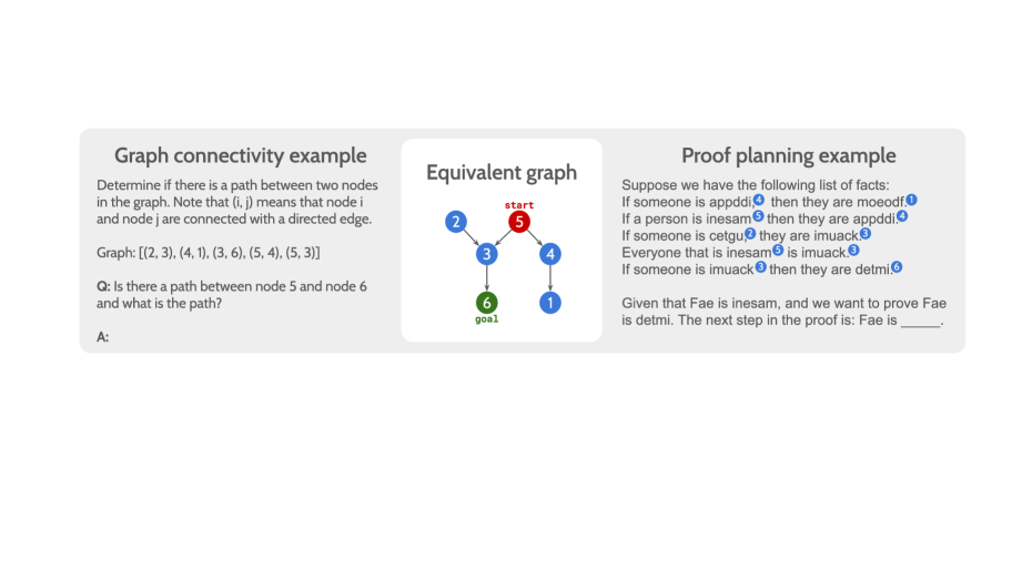
There are many reasoning tasks that can be used for evaluation. Since we endeavor to measure model reasoning ability vs complexity, we need a task for which examples are easily generated synthetically, a well-defined metric of complexity is available, and each example is not intractably difficult (i.e., where the number of required steps is polynomial in the complexity). Graph connectivity is a task where the goal is to find a path between two nodes in a graph. We choose to use the graph connectivity task since it is intuitive, it can be solved in linear time with respect to the problem complexity, and the problem complexity is readily controllable. This also allows us to controllably test for generalization at different example complexities while maintaining a reasonable context size (in order to avoid accuracy drops due to context limits rather than errors in reasoning; Modarressi et al. 2025).

We also use a simple proof planning task in deductive reasoning. Here, each example contains a list of facts of the form “if $A$ then $B$” (e.g., “If someone is a cat, then they are a mammal”). Each example also contains a start fact and a goal fact (e.g., “Given Gwendolyn is a cat, we want to prove that Gwendolyn is warm-blooded”). The model is then queried to give the next step in the proof. Examples of this task are equivalent to examples of graph connectivity, where each node in a graph can be mapped to a clause (e.g., $v_{1}$ is mapped to “someone is a cat”), and each edge is mapped to a fact (e.g., the edge $v_{1}\to v_{2}$ is mapped to “If someone is a cat, then they are a mammal”). Thus, we are able to generate proof planning examples by first generating a graph connectivity example, and then mapping each into natural language (see Section A.3 for details). Since these examples are expressed in unstructured natural language, they are not easily solved programmatically, and similarly, it is more difficult to automatically evaluate the model output. Due to this, in addition to the fact that proof planning examples are substantially longer, we simplify this task: Rather than asking the model to generate the full proof, we only require it to produce the next proof step.

3.2 Reasoning Task Complexity

In order to test models on examples of higher complexity, we require a well-defined measure of the complexity of reasoning examples. To do so, we consider the graph analogy of the proof planning task: In order to find the next step along the path from the start node to the goal node, a model must search for paths between the two nodes. A common and intuitive way to measure the complexity of a graph search task is by the distance from the start node to the goal node. A simple breadth-first search (BFS; Algorithm 1 in Section A.2) can be used to compute the distance from the start node to the goal node. However, a sufficiently powerful model could learn a more efficient algorithm to find the next node along the path from the start to the goal node. Consider a chain graph (a graph of nodes connected one after the other) in which the distance from the start to the goal node is $d$. A more clever model could surmise that since the start node has only one child, there is only one possible next node toward the goal. Such a model would find the correct next step in this search problem trivially (termed the “Clever Hans cheat” in Bachmann and Nagarajan 2024). Therefore, we use the lookahead metric $L$ from Saparov et al. (2025) to measure the complexity of this task, which is defined as the number of BFS iterations required to determine the next correct node along the path from the start node to the goal node, where the search stops early whenever it determines that any path to the goal must pass through one of the children of the source node. Algorithm 2 in Section A.2 demonstrates how to use BFS to compute the lookahead. In other words, for chain graphs the lookahead is simply 1 since the model only needs one BFS iteration to determine that there is only one correct answer. In Figure 1, the model must perform 2 BFS iterations from the start node to determine whether to proceed to node 3 or to node 4. Closely related to lookahead, the number of branches $B$ is defined as the number of outgoing nodes from the start node. Examples with larger $B$ may be more difficult as there are a larger number of possible next steps and random guessing is less effective.

4 Evaluating Models on Highly Complex Reasoning

In this section, we determine how LLMs and LRMs perform on aforementioned reasoning tasks with increasing complexity.

4.1 Models and Data

Models

LRMs are trained via reinforcement learning with verifiable rewards DeepSeek-AI et al. (2025). We evaluate a handful of LLMs and LRMs: (1) DeepSeek’s R1 (LRM), (2) its base model V3 (LLM), (3) OpenAI’s o3-mini (LRM), and (4) GPT-4o (LLM). We also evaluate the full version of o3 on small subsets of DeepRD, due to budget constraints. See Section A.1 for all model settings.

NLGraph

The first dataset we evaluate on is NLGraph (Wang et al., 2023a), which is a benchmark designed to test graph reasoning in LLMs across many tasks, including graph connectivity. The examples in NLGraph were generated using the Erdős–Rényi distribution (Erdös and Rényi, 1959). Each of the resulting graphs were transformed into an LLM input with the graph expressed as a list of edges. The test cases are split into easy, medium, and hard categories in terms of difficulty (by node count). In the hard category, there are 7770 graphs.

We emphasize that despite the fact that graphs in NLGraph-hard have a large number of nodes, the examples are fairly simple in terms of lookahead. Since the lookahead of any example is bounded above by path length, the expected lookahead is less than or equal to the expected path length. The average path length in Erdős–Rényi graphs is $\frac{\log N-\gamma}{\log(pN)}+\frac{1}{2}$ where $N$ is the number of nodes, $p$ is the edge probability, and $\gamma$ is the Euler-Mascheroni constant (Eq. 16 in Fronczak et al. 2004). Since $p\geq 0.3$ and $N\geq 26$ in NLGraph-hard, the expected lookahead of NLGraph-hard examples is bounded by $\sim 1.805$. We only evaluate the reasoning models on the hard problems for brevity.

Deep Reasoning Dataset (DeepRD)

Saparov et al. (2025) shows that transformers fail to learn to search on graphs with large lookaheads, and model scale does not alleviate this limitation. In order to test this claim for LLMs and LRMs, we modify the data generation process from Saparov et al. (2025) to generate graph connectivity examples with many lookaheads (ranging from 2 through 800). Saparov et al. (2025) does not aim to generate graphs that approach the same size as ours, even though we use their formulations of complexity as the foundation of our evaluation method. We modify the original generation process to more efficiently generate very large graphs and to reduce the likelihood of generating isomorphisms due to star patterns (graph with single central node with independent branches). We also provide a framework around this algorithm to enable a tightly controlled, depth-parameterized testbed. For each lookahead, and for each branch size $B\in\{2,4,8,16\}$, we generate an example. We take care not to generate isomorphic graphs by utilizing the NetworkX function faster_could_be_isomorphic Hagberg et al. (2008). We sample until every branch-lookahead pair has 10 examples. We also generate chain graph examples—where each graph is linear, consisting of a single path (i.e., branch size $B=1$)—with a variety of depths (ranging from 2 through 1536) for further analysis. In these chain examples, the only step required of the model should be to find the next connected node (no search or backtracking is required). Because of these steps, our dataset is also designed to detect when the model relies heavily on search heuristics. We believe a model which is overly reliant on search heuristics to the detriment of accuracy should be considered lacking in reasoning ability. Once the examples are sampled from the generator, we convert them into textual prompts, as in NLGraph (Figure 1). We also convert each example into a proof planning example, as described in Section 3.1. In total we generate 2220 examples for evaluation. For future experiments, the same data generation process can be used to generate indefinitely more graphs. We release this evaluation data, and the generation process, as the Deep Reasoning Dataset (DeepRD).

4.2 Reasoning about Graph Connectivity

Original (text-davinci-003)
Prompting	Accuracy
Zero-shot	63%
Few-shot	77%
CoT	77%
0-CoT	69%
CoT+SC	83%

New (Multiple Models)
Model	Accuracy
GPT-4o	75%
o3-mini	99%
DeepSeek V3	79%
DeepSeek R1	96%

Table 1: (left) The original average accuracies on NLGraph-hard obtained by Wang et al. (2023a); using text-davinci-003 as the model where the model is asked to determine whether or not a path exists. (right) The average accuracies of various models on the same data where we ask the model to provide a full path. We find the results of the reasoning models, even with stricter requirements, to be significantly better than text-davinci-003 augmented with chain-of-thought (CoT) and self-consistency (SC) prompting.

Figure 2: We evaluate the models V3, R1, 4o, o3-mini, and o3 on reasoning about graph connectivity. We show the average full path accuracy for each $B,L$ pair, for $B=2,4,8,16$ and $L$ between 2 and 800.

We establish the baseline performance for graph reasoning as a function of the lookahead complexity measure. First, we show the performance of the LRMs and LLMs on NLGraph-hard (Figure 1). We observe that LRMs do significantly better on the connectivity problem compared to LLMs, achieving near-perfect scores. However, as we noted earlier, the lookahead of NLGraph examples are small. So, we want to determine how the performance of LRMs scale on examples with larger lookaheads. In order to do so, we generate graphs using fixed lookaheads of increasingly larger size.

Evaluation

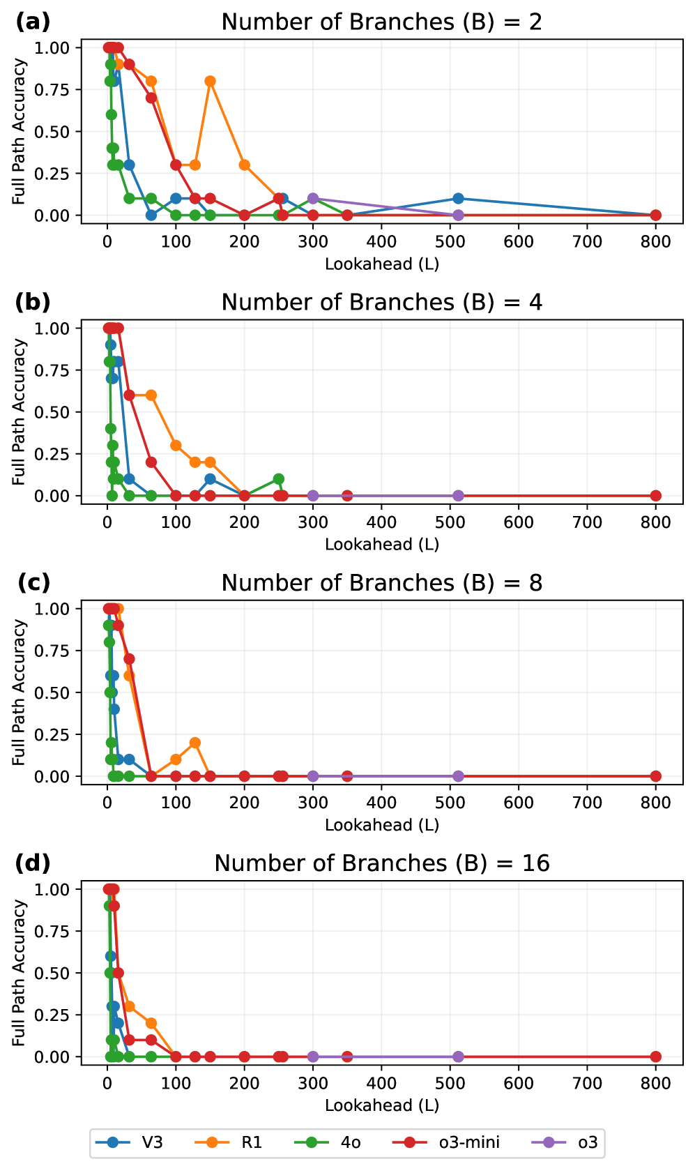
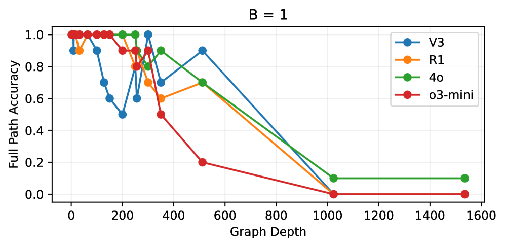
We use full path accuracy as our primary metric. Critical differences between our evaluation and the one done by Wang et al. (2023a) are that (i) we require a valid path to be produced in addition to the yes/no answer, and that (ii) the goal node is always reachable from the start node. We use a simple GPT-4o-mini prompt to extract the path from the model’s final answer (token after the “thinking end” token). We see in Figure 2 that all models drop in performance abruptly and collapse to 0 accuracy, with the drops occurring at smaller lookaheads $L$ as the number of branches $B$ increases. We also see that the reasoning models (R1 and o3-mini) drop in performance at higher $L$ than the LLMs. We measure the rate at which the models hallucinate non-existent edges (Section A.6) and find it to be quite high (over 50% in some cases) but generally trends downwards as $L$ increases. This is due to the model incorrectly concluding that there is no path, or the predicted path is incomplete. LRMs, however, have a much lower edge hallucination rate. We also ran the full o3 model on lookaheads 300 and 512. Similar to the smaller models, o3 gets 10% accuracy for $B=2$ and otherwise collapses to 0 accuracy.

Trivial Complexity

We also control for complexity due to search by looking at model performance on graphs with no branches ($B=1$), while increasing graph depth (Figure 3). We show that when we simplify the task to this trivial complexity, the models perform significantly better than the $B=2$ case, but still quickly drop in performance for large depths (Figure 3). Even in this extremely simple reasoning task, the models fail to truly generalize.

Figure 3: For the graph connectivity problem, we show the average full path accuracy for test cases with graph depths between 2 to 1536, when constraining the graph to be a chain graph (one node after the other).

Figure 4: For the graph connectivity problem, we show the average token completion count for $B=8$ and $L$ between 2 and 800. We can only run the large o3 on a small range of $L$ due to budget constraints.

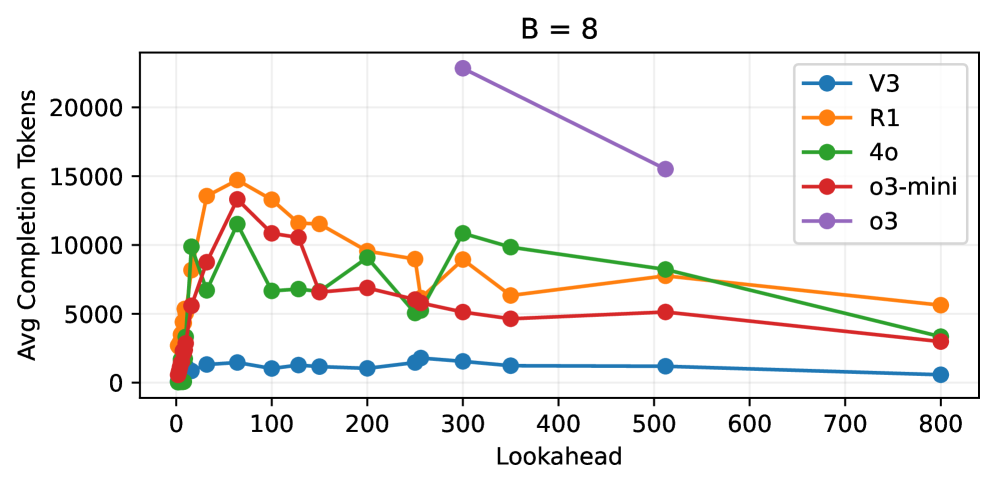
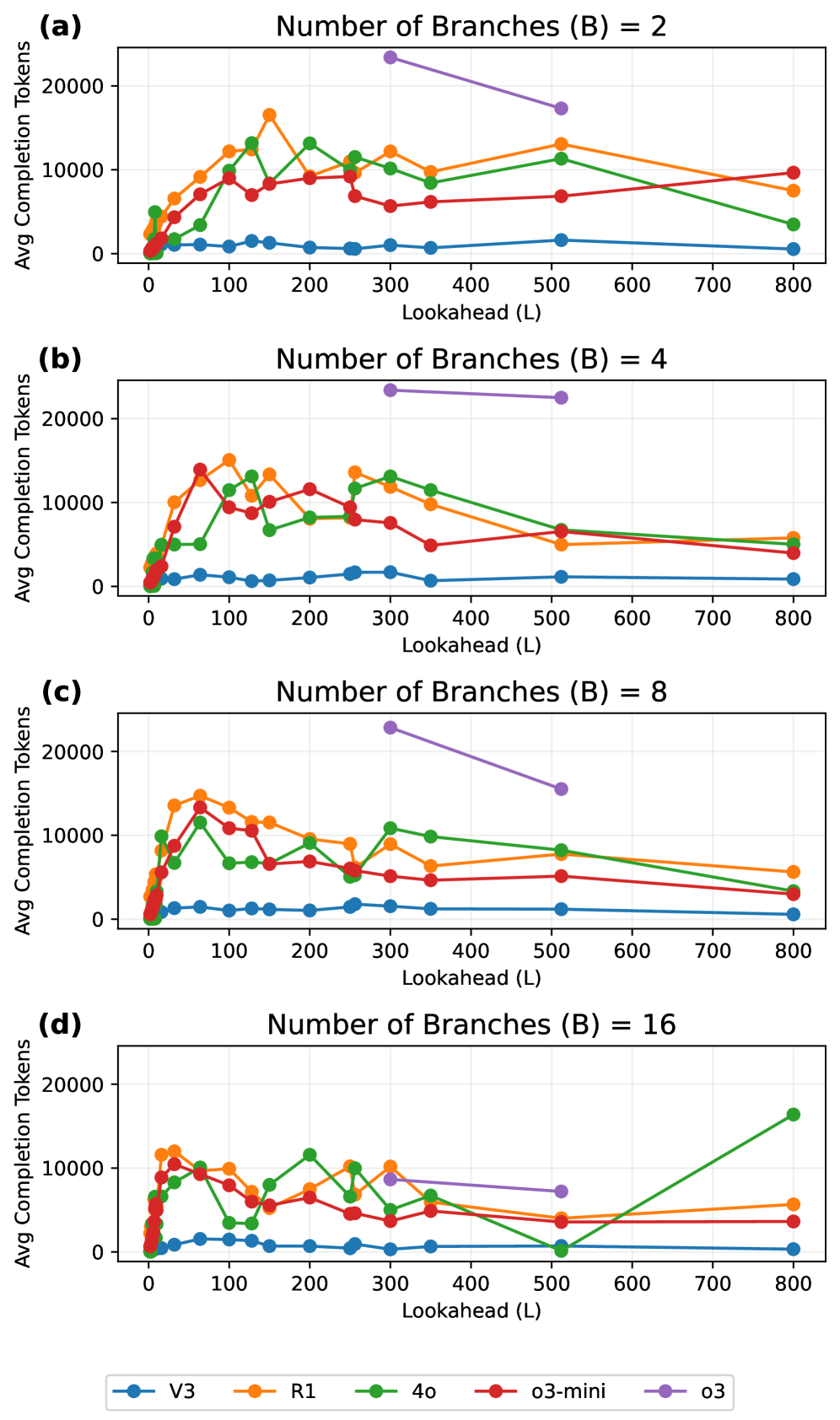
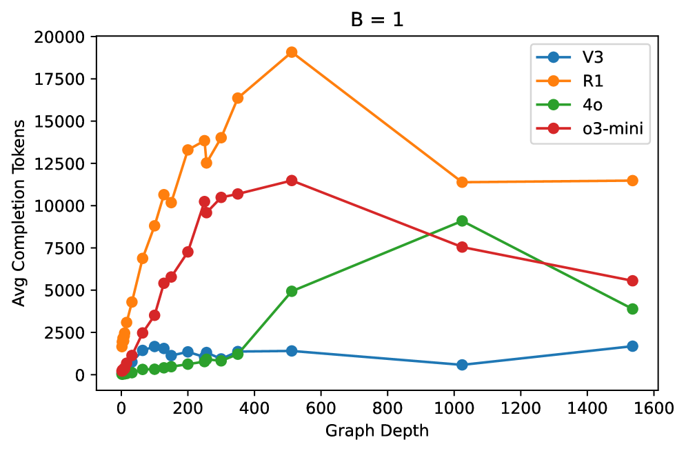
Token Usage

Lawsen (2025) claimed that the LRM analysis of Shojaee et al. (2025) was unfair due to token limits, which would limit the model’s ability to work through reasoning problems. Our analysis shows that token limits do not cause the drops in accuracy. While the LLMs (V3, 4o) did hit length limits throughout the set of lookaheads, the LRMs (R1, o3-mini) rarely hit length limits (Section A.6). We inspected the “stop_reason” field in every model response. In fact, the completion token usage seems to decrease with increasing lookahead (Figure 4). Results for all branches are shown in Section A.7. Manual inspection of the LRM responses for more complex examples also seems to indicate no information is being truncated, as edges from the very beginning of the prompt are present in the output. Interestingly, if the nodes in the inputs for the trivial complexity evaluation were presented in the order of correct traversal, all models achieve near-perfect performance. This further indicates the models are limited by reasoning ability, and not by token limits.

4.3 Proof Planning in Deductive Reasoning

Next, we evaluate the reasoning ability of LRMs via proof planning, by rendering each example as a natural language proof planning problem.

Figure 5: We evaluate the models on the proof planning task. We show the average next step prediction accuracy for each $(B,L)$ pair, for $B=2,4,8,16$ and $L$ between 2 and 800.

Figure 6: Histograms of lookahead and number of branches metrics for ConceptNet, ogbl-wikikg2, ogbn-papers100M, ogb, and NaturalProofs. There is no direct measure for number of branches for NaturalProofs since it is a dataset of proofs rather than graphs. The top row is lookaheads in log scale and the bottom row is number of branches in log scale. The red lines represent the $50^{th}$, $75^{th}$, $90^{th}$, $99^{th}$, and $99.9^{th}$ percentiles respectively.

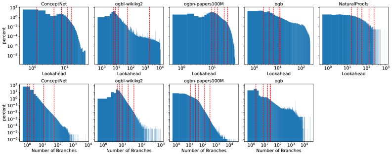
Figure 5 shows that the characteristic performance cliffs observed in the graph connectivity setting persist in the proof planning setting, and indeed the cliffs appear at lower complexities. Between lookaheads $L=10$ and $L=64$, R1 and o3 accuracies start collapsing for branch size $B>1$, though they still collapse at larger lookaheads than V3 and 4o. Although accuracy for $B=2$ and $B=4$ cases seems to stay above zero even as lookahead increases, this residual performance is not indicative of genuine reasoning ability. Rather, for a given number of branches $B$, the model can resort to a uniform random guess, achieving success with probability $1/B$. For $B=2$ we can see the performance hovering around $\frac{1}{2}$, and for $B=4$, we can see the performance hovering around $\frac{1}{4}$. Empirically, models that produce fewer “thinking” tokens tend to have non-zero accuracy for branches 2 and 4, and a somewhat extended plateau for branches of size 8 and 16. In fact, we can also observe this $1/B$ accuracy trend for 4o in the symbolic case for $B=2$ (Figure 15 in Section A.7). The full o3 model also seems to converge to chance when run on lookaheads $L=300$ and $L=512$ and number of branches $B\in\{2,4,8,16\}$ (Figure 5) despite using a large number of tokens (Figure 17 in Section A.7). It is difficult to perform deeper analysis since we do not have access to the reasoning tokens of o3. This behavior reflects stochastic guessing in LRMs rather than enhanced reasoning capabilities.

Among the models evaluated, 4o attains the highest apparent accuracy solely by emitting very concise outputs—fewer than ten tokens on average—which we hypothesize leads the model to perform uniform random guessing more often and attain $1/B$ accuracy. By contrast, V3, despite also not being trained with reasoning incentives, generates verbose justifications that may discourage it from performing random guessing (Figure 5 in Section A.7). The reason for V3’s markedly higher token usage in the natural-language setting, relative to its behavior for symbolic graphs (Figure 4), remains unclear.

Verification of Real-World Proofs

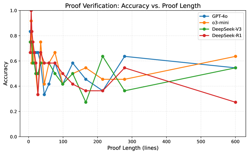
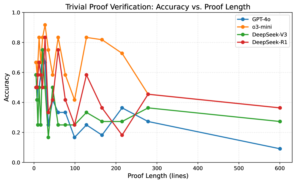
We evaluate the LRMs’ ability to find errors and validate proofs using the NaturalProofs dataset. We structure this problem to evaluate the model’s ability to (1) traverse the in-context proof DAG, (2) verify that each step is properly licensed by its premises, and (3) confirm that the conclusion is supported (i.e., the path is valid end-to-end), all in a natural reasoning setting. We first sample proofs via stratified sampling over proof length, ensuring balanced coverage across short, medium, and long proofs. For each sampled proof, we randomly sample a line in the proof to introduce a minimal but semantics-altering edit while preserving surface form (e.g., changing a quantifier, negation, inequality direction, number/variable/name). The modified proof is then given to the model with full proof context and is prompted to (1) judge whether the proof is correct and (2) if incorrect, identify the erroneous line. We note that, because this dataset is real-world natural language, it is quite noisy. We calculate accuracy of error finding and report the accuracy along the axis of proof length (Figure 21). We also carry out the trivial experiment of finding errors in unmodified proofs and see that the model performance can still suffer due to dataset noise or erroneous error identification (Figure 22). This suggests that our perturbation procedure is not the sole driver of the collapse. Looking at the metrics, we find patterns mirroring performance on synthetic graphs—namely, the performance abruptly drops at larger depths. Perturbation examples and proofs can be found in Table 4 of Section A.8.

4.4 Inspection of Failure Modes

We wish to gain insight into the failure modes of the models, by manually inspecting the “thinking tokens” of R1 (such tokens are unavailable for o3 and o3-mini). To that end, we sampled a number of symbolic graphs with $L\geq 300$ and $B=3$ for which R1 returned no path and a number of symbolic graphs for which R1 returned an incorrect path, we manually inspected the thinking tokens with those inputs, and categorized the mistakes according to a number of error types:

• The model omits a necessary and previously-stated outgoing edge at some intermediate step (this occurred in 15/20 samples). Example of thinking trace: “Similarly, from 860: (860, ?) — I see (860, 227) ? (860, 227) is not listed”.

• The model misses one of two outgoing edges of the start node, thus ignoring one of two branches entirely (5/20 samples). Example of thinking trace: “First, find all edges starting from 220. Looking at the list, I see (220, 723). That’s the only one with 220 as the start.”

• The model hallucinates an edge at some intermediate step (2/20 samples).

Under type I and type II errors, after the graph misses the required outgoing edge, thus pruning the gold branch, the model proceeds correctly on the wrong branch, and subsequent steps are locally consistent, leading to a “no path” response. For the examples for which the model returned an incorrect path, we find that Type III errors occurred most frequently (13/20 for Type I, 3/20 for Type II, 16/20 for Type III). In this case, the model often makes Type I and Type III errors simultaneously (11/20 cases) to derive a path which travels through the wrong branch, thus leading to an incorrect path result. These main failure modes from our analysis aligns with the notion of “propagation error” in Dziri et al. (2023): after a single early local misstep, later computations are correct, conditioned on incorrect parent values. Their analysis found a similar conclusion of such “propagation errors” contributing to the decrease in the proportion of “fully correct” answers as depth increases.

5 Complexity of Real-World Reasoning

In this section, we aim to relate LRM behavior to the structural complexity of graphs and proofs that occur in real-world scenarios. This connection allows us to estimate where LRMs will succeed (the “head” of the distribution of lookahead and number of branches) and where they will predictably fail (the “tail”) on real-world reasoning problems.

Real-World Datasets

We analyze a diverse suite of large, real-world graphs. Most are drawn from the Open Graph Benchmark (OGB; Hu et al., 2020), which includes code ASTs, academic citation networks, biomedical interaction graphs, and more. We also include ConceptNet (Speer et al., 2017), a single integrated knowledge graph compiled from multiple sources, and the NaturalProofs corpus of formal proofs (Welleck et al., 2021). We analyze the distributions of ConceptNet, ogbl-wikikg2, ogbn-papers100M, and NaturalProofs independently; and aggregate the other 24 OGB datasets into a single distribution (normalized uniformly across datasets) called ogb.

Measures

For each dataset, we compute (i) the lookahead from every node to every other node using an efficient algorithm (Algorithm 3 in Section A.2). When this is computationally infeasible, we uniformly sample a large set of source nodes (e.g., 2M for ConceptNet and 30k for ogbn-papers100M) and compute lookaheads to all nodes. We also compute (ii) the number of branches (i.e., out-degree) of all nodes. For proofs such as those in NaturalProofs, the proof length (in terms of the number of steps) serves as a measure of complexity analogous to lookahead. This is due to the fact that for a sufficiently powerful formal system (e.g., including deduction rules for quantifiers, or arithmetic), there will often exist logical forms for which an infinite number of deductions are possible (e.g., given $x=y$, we can conclude $xz=yz$ for any $z$; or given $\forall x.f(x)$, we can conclude $f(a)$ for any term $a$). Thus, the number of “branches” at many nodes in a proof is infinite, and for any proof consisting of $n$ steps, there will almost always exist a disjoint proof with a different goal of unbounded length (i.e., sharing no proof steps with the original proof). In NaturalProofs, the proofs are given as a list of lines (in Lean or unstructured natural language) and we treat the number of lines as a proxy for proof length, which is analogous to lookahead.

Summary statistics

As seen in Figure 6, if each pair of nodes in a graph is taken as a graph connectivity example, the vast majority of examples seen in empirical graphs have quite low complexity. In our model evaluations for reasoning on graph connectivity (Figure 2), we see the accuracy drop at around $L=100$ through $200$—sooner for high $B$. For ogbl-wikikg2 and ogb, $L=100$ examples are in the $99^{th}$ percentile. Similarly, we see the LRM performance on next step prediction for proof planning collapses around $L=16$ through $32$ (Figure 5) and we see that for NaturalProofs, $L=16$ and $L=32$ fall at the $50^{th}$ and $75^{th}$ percentile respectively. We also see that for all datasets, examples with number of branches $B=7$ fall in the $75^{th}$ percentile and there are datasets with branch counts in the thousands—well outside of the success regime of LRMs.

6 Discussion

We began by comparing LLMs and LRMs on the NLGraph benchmark, where LRMs outperformed LLMs—but only on low‑complexity graphs. We tested the models on examples with larger lookaheads and number of branches, and found that every model suffered an abrupt drop in accuracy. This performance cliff persisted even in examples with chain graphs (no search or backtracking), demonstrating that limitations in reasoning—not token limits or truncation—drive the collapse.

Extending this to natural language proof planning yielded the same result: LRM performance collapses as proof complexity increases, and in fact, the performance cliff appears at even smaller lookaheads than in the graph connectivity setting.

Finally, by measuring lookahead and branching distributions over real‑world graph and proof corpora, we showed that although most queries lie within the LRMs’ success regime, a long tail of harder instances falls squarely beyond LRM capabilities. This mirrors prior work showing steep drops when test complexity exceeds training complexity (Dziri et al., 2023; Lee et al., 2025), and suggests that current LRMs remain tightly bound to their training distribution rather than exhibiting robust, human‑like generalization.

7 Conclusion

Current state-of-the-art LRMs excel on the relatively simple reasoning tasks that comprise much of existing benchmarks and real-world datasets, but falter once tasks become sufficiently complex. DeepRD enables exploration of the limits of LRM reasoning ability for both graph connectivity and proof planning, revealing abrupt failures that likewise appear in the long-tail of real-world reasoning tasks. Bridging this gap will require new methods to encourage more robust out-of-distribution generalization in reasoning.

DeepRD enables several interesting future research directions. First is a deeper analysis R1’s “thinking” tokens for traversal and reasoning: Are there any thinking patterns that are predictive of the model’s performance? Another, enabled by unlimited data generation, is to test whether fine-tuning models on higher complexities in symbolic cases transfer performance to natural language reasoning.

Limitations

One of our primary limitations is lack of open access to OpenAI’s o3 and o3-mini, or their training details. Running qualitative analysis on the thinking tokens of the OpenAI models would give a better idea of consistent failure modes across all LRMs. Also, given the high cost to run inference on state-of-the-art LLMs, and especially LRMs due to increase in token usage, another limitation is running the evaluation on more test cases. Currently we have a set of lookaheads and number of branch pairs we evaluate on, and that set can be made much larger with more evaluation budget. The budget also limited us to graph connectivity and next step prediction, but our methodology can be applied to other graph and reasoning problems. Finally, open access or even details for the training data of the LLMs and LRMs (for both DeepSeek and OpenAI) would allow us to analyze the complexity of the complete training distribution.

Appendix A Appendix

A.1 Model Settings

A.1.1 System Prompt

The following system prompt was used for all models:

“When answering a yes or no question, always start the answer with |YES| or |NO| depending on your answer.”

All models were run with a temperature setting of 0, except for the OpenAI reasoning models where the API does not allow customization of the temperature.

A.1.2 Models Used

The experiments utilized the following models:

From Together.ai:

We used the API from https://www.together.ai/ for the two models:

• deepseek-ai/DeepSeek-R1 (version 0528); 685B parameters

• deepseek-ai/DeepSeek-V3 (version 0324); 671B parameters

From OpenAI:

We used the API from https://platform.openai.com/ for the four models below. We have no knowledge of any official model sizes (i.e., number of parameters).

• gpt-4o-mini-2024-07-18 (for extracting paths from the final answer)

• o3-mini-2025-01-31

• o3-2025-04-16

• gpt-4o-2024-08-06

A.2 Computing Lookahead

Given a start vertex $s$ and a goal vertex $g$ in a directed graph, we define lookahead as the number of breadth-first search (BFS) iterations needed to determine the next vertex along a path from $s$ to $g$. Alg. 1 provides pseudocode for a simple BFS implementation.

We can minimally modify the BFS algorithm to compute the lookahead, as described above, which is shown in Alg. 2. Intuitively, we essentially perform BFS until we either: (1) find the goal $g$, or (2) determine that any path from $s$ to $g$ must pass through a child of $s$. Alg. 2 keeps track of, for each node in the frontier, which child of $s$ can reach it; as soon as all surviving paths to $g$ must pass through the same child of $s$, we stop and return that layer index $L$ (the required lookahead). We use this to compute lookahead, our main measure of graph complexity, as explained in Section 3.2.

In our analysis, we need to be able to compute the lookahead between many pairs of nodes in a given graph. While applying Alg. 2 for each pair is a valid approach, it can be costly in terms of running time. Therefore, we can modify the algorithm to compute the lookahead from a source $s$ to all possible targets. We observe that Alg. 2 only depends on the target $g$ at the first step within each iteration, and so we can modify this part of the algorithm to compute the lookahead to all possible targets, which is shown in Alg. 3.

In our analysis, we similarly need to compute the all-pairs shortest-path lengths for a given graph. We implement a simple approach to do so in Alg. 4. This algorithm essentially runs BFS iteratively for all pairs of vertices.

1function distance(source node $s$, goal node $g$)

2    if $s=g$ return 0

3    initialize $d=1$

4    initialize $Q=\{c:c\text{ is a child node of }s\}$

5    while $Q$ is not empty do /* BFS main loop */

6       if $g\in Q$ return $d$

7       set $Q=\{c:c\text{ an \emph{unvisited} child of any }v\in Q\}$

8       set $d=d+1$

9      

10   return $\infty$

Algorithm 1 Breadth-first search to compute the distance from node $s$ to node $g$.

1function lookahead(source node $s$, goal node $g$)

2    if $s=g$ return 0

3    initialize $l=1$

4    initialize $R_{v}=\varnothing$ for all nodes $v$

5    initialize $Q=\{c:c\text{ is a child node of }s\}$

6    set $R_{c}=\{c\}$ for every child node $c$ of $s$

7    while $Q$ is not empty do /* BFS main loop */

8       if $g\in Q$ return $l$

9       else if $c\in R_{v}$ for all $v\in Q$ for some child $c$ of $s$

10          return $l$

11      for $v\in Q$ and every child node $c$ of $v$ do

12          set $R_{c}=R_{c}\cup R_{v}$

13         

14      set $Q=\{c:c\text{ an \emph{unvisited} child of any }v\in Q\}$

15       set $l=l+1$

16      

17   return $\infty$

Algorithm 2 Algorithm to compute the lookahead from node $s$ to node $g$.

1function lookaheads_from_src(source node $s$)

2   

3   initialize $l=1$

4    initialize $L_{v}=\infty$ for all nodes $v$

5    initialize $R_{v}=\varnothing$ for all nodes $v$

6    initialize $Q=\{c\mid c\text{ is a child of }s\}$

7    set $R_{c}=\{c\}$ for every child node $c$ of $s$

8   

9   while $Q$ is not empty do /* BFS main loop */

10       if $c\in R_{v}$ for all $v\in Q$ for some child $c$ of $s$

11          break

12         

13      for $v\in Q$ and every child node $c$ of $v$ do

14          set $R_{c}=R_{c}\cup R_{v}$

15         

16      set $L_{v}=l$ for all $v\in Q$

17       set $Q=\{c:c\text{ an \emph{unvisited} child of any }v\in Q\}$

18       set $l=l+1$

19      

20   

21   foreach $v$ is any descendant of a node in $Q$ do

22       set $L_{v}=l$

23      

24   

25   return $L$

26   

Algorithm 3 Computes the lookaheads from a given source node $s$ to all other nodes in the graph. In our experiments, we add an additional loop over source nodes $s$, in order to compute the lookaheads between all pairs of nodes.

1function pairwise_distance(graph $G$)

2    initialize $\mathit{Dist}=$ empty counter

3    /* distribution of pairwise shortest-path lengths */

4   [2pt]

5   foreach node $s$ in $G$ do

6       initialize $\mathit{visited}=\{s\}$

7       initialize $Q=\{c\mid c\text{ is a child of }s\}$

8       initialize $d=1$

9      

10      while $Q$ is not empty do /* BFS main loop */

11          foreach $v\in Q$ do

12             add one occurrence of $d$ to $\mathit{Dist}$

13             add $v$ to $\mathit{visited}$

14            

15         set $Q=\{c\mid c\text{ is a child of any }v\in Q\text{ and }c\notin\mathit{visited}\}$

16          set $d=d+1$

17         

18      

19   return $\mathit{Dist}$

20   

Algorithm 4 Computes the distribution of shortest-path distances between all pairs of nodes in $G$.

A.3 Translating from Symbolic Query to Proof Planning

1

2function graph_to_logic(edge list $E=[(A,B)]$, query $(X,Y)$, where $A,B,X,Y$ are integers representing the nodes)

3   

4   initialize $V=$ unique nodes appearing in $E$

5    initialize $n=|V|$

6   

7   initialize $name=$ a random name

8    initialize $Adjs=$ list of $n$ distinct random attributes

9    /* attributes are random two-syllable words */

10   sort $V$ into $[v_{0},\dots,v_{n-1}]$

11   

    initialize $Choices=$ array of eight strings:

12    1. “If $name$ is $adj\_A$, then $name$ is $adj\_B$.”

13    2. “$name$ is $adj\_A$ implies $name$ is $adj\_B$.”

14    3. “$name$ is $adj\_B$ is true if $name$ is $adj\_A$.”

15    4. “$adj\_B$ is true if $adj\_A$ is true.”

16    5. “If $adj\_A$ then $adj\_B$ is true.”

17    6. “If $adj\_A$ is true then $adj\_B$.”

18    7. “Given $name$ is $adj\_A$ then $name$ is $adj\_B$.”

    8. “If a person is $adj\_A$ then they are $adj\_B$.”

19   initialize $Preds=\varnothing$

20   

21   foreach $(A,B)\in E$ do

22       set $adj_{A}=Adjs[A]$

23       set $adj_{B}=Adjs[B]$

24       initialize $predicate=$ random string from $Choices$.

25       append $predicate$ to $Preds$

26      

27   

28   initialize $adj_{X}=Map[X]$,

29    initialize $adj_{Y}=Map[Y]$

30    $Q\leftarrow$ “Given that name is adj_X, and we want to prove name is adj_Y. The next step in the proof is: name is xxx.”

31   

32   return $Preds,\;Q$

33   

Algorithm 5 Translate an edge list and a query $(X,Y)$ into natural-language predicates and a fill-in-the-blank logic question.

We wish to translate the graph search query from symbolic to natural language proof planning. We do this by first choosing a random name (e.g., Alyssa), which we use as the subject for the natural language query. We then assign each node a unique attribute, which is a fake two-syllable word. Each syllable consists of one of the following forms: Consonant (C) + Vowel (V), VC, CVC, CVV, CCV, VCV, or VCC. Examples of these attributes are "movo", or "retil", etc. Then each directed edge is turned into a predicate involving two attributes, such as "If Alyssa is movo, then Alyssa is retil or Alyssa is movo implies Alyssa is retil", etc. We use eight different predicate forms to introduce linguistic variety. The query itself, consisting of a start and goal node, is also translated into natural language. The pseudocode which describes this process is provided in Alg. 5.

A.4 Graph Sampling

1

2function generate_lookahead_graphs(dataset size $N$, lookahead $l$, branches $b$, max edges $m$)

3    initialize $\mathcal{D}=\varnothing$

4   

5   while $|\mathcal{D}|<N$ do

6       set $n=\max(2,1+b\cdot l+\text{random}(0,m/3))$

7       initialize vertices $V=\{v_{0},\ldots,v_{n-1}\}$, edges $E=\varnothing$

8      

      /* Build main path */

9       for $i=0$ to $l-1$ do

10          $E\leftarrow E\cup\{(v_{i},v_{i+1})\}$

11         

12      set start $s=v_{0}$, goal $g=v_{l}$

13      

      /* Add alternative branches */

14       set $k=l+1$

15       for $j=1$ to $b-1$ do

16          $E\leftarrow E\cup\{(v_{0},v_{k})\}$

17          set branch_length $=l+\text{random}(0,\min(2,n-k))$

18          for $i=1$ to branch_length $-1$ do

19             $E\leftarrow E\cup\{(v_{k+i-1},v_{k+i})\}$

20            

21         $k\leftarrow k+$ branch_length

22         

23      

      /* Preferential attachment phase */

24       initialize valid_paths $\mathcal{V}=$ descendants of $v_{1}$

25       for remaining vertices $v_{new}$ do

26          if $|E|\geq m$

27            break

28         

29         sample $d_{in},d_{out}\sim(d+1)^{-1}$

30         

31         select children $\mathcal{C}\subseteq V$ with preferential_attachment(in-degree)

32          connect $v_{new}$ to each child in $\mathcal{C}$

33         

34         compute valid parents avoiding cycles

35          select parents $\mathcal{P}\subseteq V$ with preferential_attachment(out-degree)

36          connect each parent in $\mathcal{P}$ to $v_{new}$

37         

38         if compute_lookahead($s,v_{1},g$) $\neq l$

39             rollback edges for $v_{new}$

40            

41         

42      

      /* Finalization */

43       remove excess edges while preserving paths from $s$ to $g$

44       shuffle node IDs

45      

46      find shortest path $P$ from $s$ to $g$

47       if $P$ does not exist or $|P|\leq 2$

48         continue

49      

      /* Validation */

50       if out-degree$(s)\neq b$

51         continue

52      if multiple simple paths exist from $s$ to $g$

53         continue

54      if graph isomorphic to any in $\mathcal{D}$

55         continue

56      if exists path shorter than $l$ from $s$ to $g$

57         continue

58      

      /* Create single training example from first step */

59       set $v_{curr}=P[0]=s$, $v_{next}=P[1]$

60       if compute_lookahead($v_{curr},v_{next},g$) $=l$

61          if only one child of $v_{curr}$ has path to $g$

62             add $(E,s,g,v_{next})$ to $\mathcal{D}$

63            

64         

65      

66   

67   return $\mathcal{D}$

68   

Algorithm 6 Generate graph dataset with controlled lookahead property for pathfinding tasks.

We use an algorithm (Alg. 6) that generates directed acyclic graphs (DAGs) of a specific lookahead. We begin with constructing a base graph with $n$ nodes, where $n$ is chosen to have at least $b\text{ (branches) }\cdot l\text{ (lookahead) }$ nodes and additional random nodes. A main path of length $l$ is created from node $v_{0}$ to $v_{l}$, establishing the golden route from start to goal. Then, $b-1$ alternative branches are added, each starting from the start node $v_{0}$ and having length approximately equal to $l$ with slight random variation. This ensures that from the start node, there are exactly $b$ possible initial choices, but only by looking ahead $l$ steps can a model identify which choice leads to the goal.

The preferential attachment phase adds complexity to the graph while preserving the lookahead property. New nodes are connected with a power-law degree distribution so that the probability of having degree $d$ is proportional to $(d+1)^{-1}$, determining how many edges to add. For selecting which existing nodes to connect to, the algorithm uses preferential attachment: when adding outgoing edges from a new node, it selects target nodes with probability $P(v)\propto\alpha+\text{in-degree}(v)$, and when adding incoming edges, it selects source nodes with probability $P(v)\propto\alpha+\text{out-degree}(v)$. This creates a heavy-tailed degree distribution where most nodes are sparsely connected and a few nodes become densely connected hubs. The algorithm tracks which nodes lie on valid paths from start to goal and carefully avoids creating cycles. If adding edges to a new node would reduce the lookahead below $l$, those edges are rolled back.

After construction, the algorithm performs several validation steps. Node IDs are randomly shuffled to prevent models from learning spurious correlations between topology and numbering. The graph is checked to ensure: (1) exactly one simple path exists from start to goal when considering all edges, (2) the start node has exactly $b$ outgoing edges, (3) no path shorter than $l$ steps exists from start to goal, and (4) the graph structure is not isomorphic to previously generated graphs.

A.5 Example Model Responses

Tables 2 and 3 show model outputs (reasoning + response) for sample proof planning V3 and R1 runs.

V3 model response

query:

Suppose we have the following list of facts:

If someone is eyzvih, they are tucibm.

If Mariah Gonzalez is eyzvih, then Mariah Gonzalez is ttaask.

If a person is veubte, they are uzvymi.

If Mariah Gonzalez is emkatv, then Mariah Gonzalez is rowzo.

If a person is uztio, they are otis.

Everyone that is rowzo is hatho.

…

Given that Mariah Gonzalez is moilu, and we want to prove Mariah Gonzalez is otis. The next step in the proof is: Mariah Gonzalez is ____.

Let’s break down the steps to find out what Mariah Gonzalez is next, given that she is moilu and we want to prove she is otis.

1. Given: Mariah Gonzalez is moilu.

2. From "If Mariah Gonzalez is moilu, then Mariah Gonzalez is zdedoa." $\rightarrow$ Mariah Gonzalez is zdedoa.

3. From "If someone is zdedoa, they are vupon." $\rightarrow$ Mariah Gonzalez is vupon.

4. From "If Mariah Gonzalez is vupon, then Mariah Gonzalez is xbaann." $\rightarrow$ Mariah Gonzalez is xbaann.

5. From "If someone is xbaann, they are gohsi." $\rightarrow$ Mariah Gonzalez is gohsi.

6. From "Everyone that is gohsi is uxfeyl." $\rightarrow$ Mariah Gonzalez is uxfeyl.

…

29. From step 28, Mariah Gonzalez is uztio $\rightarrow$ she is otis (which is our goal).

The next step after Mariah Gonzalez is moilu is that she is zdedoa (from step 2).

Final Answer: zdedoa

Table 2: V3 model query and reasoning transcript for a given natural language prompt.

R1 model response

query:

Suppose we have the following list of facts:

If someone is eyzvih, they are tucibm.

If Mariah Gonzalez is eyzvih, then Mariah Gonzalez is ttaask.

If a person is veubte, they are uzvymi.

If Mariah Gonzalez is emkatv, then Mariah Gonzalez is rowzo.

If a person is uztio, they are otis.

Everyone that is rowzo is hatho.

…

Given that Mariah Gonzalez is moilu, and we want to prove Mariah Gonzalez is otis. The next step in the proof is: Mariah Gonzalez is ____.

<think>

We are given that Mariah Gonzalez is moilu, and we want to prove that Mariah Gonzalez is otis.

Let’s list the facts that involve "moilu" and see what we can derive:

1. "If Mariah Gonzalez is moilu, then Mariah Gonzalez is zdedoa."

Since Mariah Gonzalez is moilu, then she is zdedoa.

2. "If someone is zdedoa, they are vupon."

So, from zdedoa, we get that Mariah Gonzalez is vupon.

3. "If Mariah Gonzalez is vupon, then Mariah Gonzalez is xbaann."

Therefore, Mariah Gonzalez is xbaann.

…

Let’s trace that:

Given: moilu -> xori (from "Each person that is moilu is xori.")

Then: xori -> emkatv (from "If Mariah Gonzalez is xori then they are emkatv.")

Then: emkatv -> rowzo (from "If Mariah Gonzalez is emkatv, then Mariah Gonzalez is rowzo.")

Then: rowzo -> hatho (from "Everyone that is rowzo is hatho.")

…

</think>

Given that Mariah Gonzalez is moilu, the goal is to prove she is otis. The path to otis involves the following chain:

- From "Each person that is moilu is xori," since Mariah is moilu, she must be xori.

- From "If Mariah Gonzalez is xori then they are emkatv," she becomes emkatv.

- From "If Mariah Gonzalez is emkatv, then Mariah Gonzalez is rowzo," she becomes rowzo.

…

Final Answer: xori

Table 3: R1 model query and reasoning transcript for a given natural language prompt.

A.6 Error Analysis

In this section, we provide additional results from analyzing the various errors we observe from the model. We categorize our analysis of these errors into symbolic and logic graphs with $B>1$, where we plot error rate vs lookahead, as well as symbolic and logic graphs with $B=1$, where we plot error rate vs graph depth, which is analogous to lookahead for single-branch (chain) graphs.

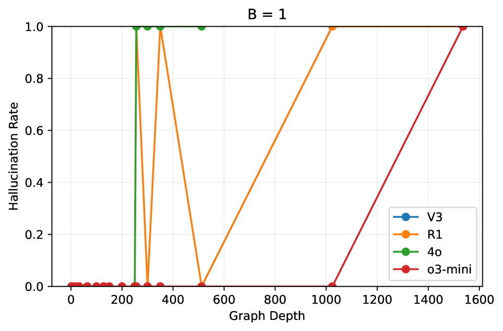
Edge Hallucination Rate

An edge hallucination is defined as the appearance of an edge in the model’s output that did not exist in the input symbolic graph. The edge hallucination rate tracks the proportion of runs per lookahead and branch size in which the model produced at least one edge hallucination. For $B>1$ (Fig. 7), rates are high at small lookaheads, drop to near zero toward medium lookaheads, then rise again at very high lookaheads. For $B=1$ (Fig. 8), rates stay near zero through moderate depths then rise sharply at large depths. The depth at which the rate begins to rise depends on the model.

Figure 7: Edge hallucination rates for symbolic graph with $B>1$.

Figure 8: Edge hallucination rates for symbolic graph with $B=1$.

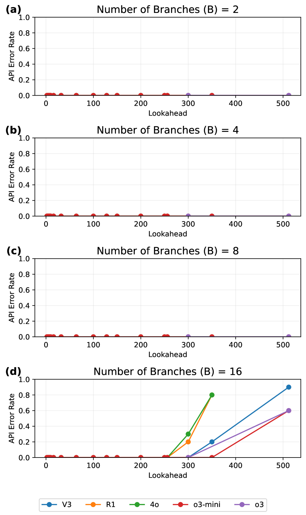
API Error Rate

A run is aborted by the API when the number of tokens needed to complete the prompt exceeds the amount supported by the API. Fig. 9 and Fig. 10 shows the proportion of these errors for the symbolic and logic graphs, respectively. In both cases, API errors only started appearing for $B=16$.

Figure 9: API error rate for symbolic graph with $B>1$.

Figure 10: API error rate for logical graph with $B>1$.

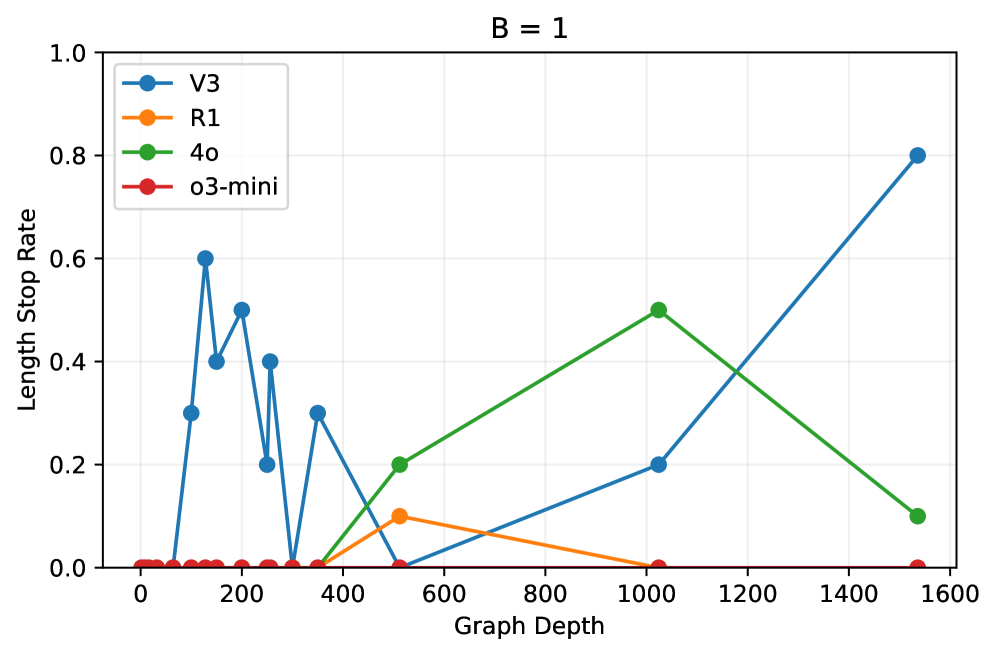
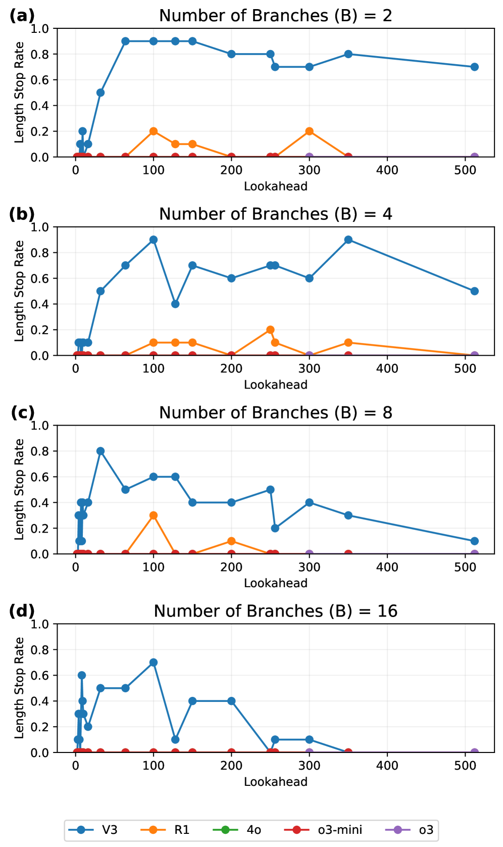
Length Stop Error

The models will abruptly stop its processing of a prompt if the amount of tokens used during processing exceeds its limit. This rate tracks the proportion of runs per lookahead and branch size which was stopped due to reaching this length limit. Our observed rates largely correlate with the completion token usage, with a rise from small lookahead into a mid-lookahead peak and then taper at larger lookahead, and varying drastically by model. This behavior is consistently observed for symbolic graphs with $B>1$ (Fig. 11), symbolic graphs with $B=1$ (Fig. 12), logic graphs with $B>1$ (Fig. 13), and logic graphs with $B=1$ (Fig. 14).

Figure 11: Length stop rate for symbolic graphs with $B>1$.

Figure 12: Length stop rate for symbolic graphs with $B=1$.

Figure 13: Length stop rate for logical graphs with $B>1$.

Figure 14: Length stop rate for logical graphs with $B=1$.

A.7 Additional Analysis

In this section, we provide some additional analysis results on model responses, namely the next step accuracy and completion tokens used. Similar to the error analysis, We categorize these into symbolic, logic graphs with $B>1$, as well as symbolic, logic graphs with $B=1$.

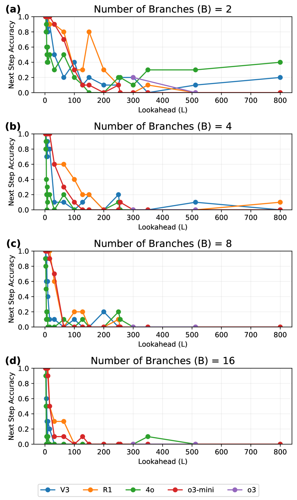
Next Step Accuracy

Next step accuracy indicates the accuracy of the model’s prediction when asked to give the next node in the shortest path from start to goal, averaged per lookahead and branch size. For $B>1$ (Fig. 15), accuracy is highest at small lookaheads and generally decreases as lookahead grows. With increasing $B$, the drop in accuracy starts a smaller and smaller and smaller lookaheads. We observe corresponding behavior for $B=1$ (Fig. 16).

Figure 15: Next step accuracy for symbolic graph with $B>1$.

Figure 16: Next step accuracy for symbolic graph with $B=1$.

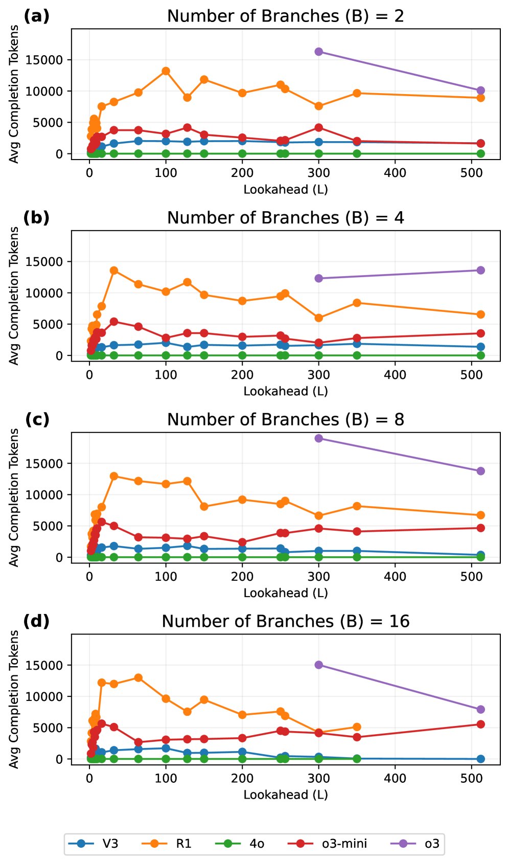
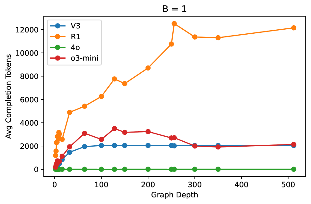
Average Completion Tokens

We plot the average number of tokens generated per prompt, which includes thinking and output tokens for reasoning models, per lookahead and branch size. The amount of tokens used vary drastically across the different models, however, across all models, counts typically rise from small lookahead into a mid-lookahead peak and then taper at larger lookahead. This behavior is consistently observed for symbolic graphs with $B>1$ (Fig. 17), symbolic graphs with $B=1$ (Fig. 18), logic graphs with $B>1$ (Fig. 19), and logic graphs with $B=1$ (Fig. 20).

Figure 17: Average completion tokens for symbolic graphs with $B>1$.

Figure 18: Average completion tokens for symbolic graphs with $B=1$.

Figure 19: Average completion tokens for logical graphs with $B>1$.

Figure 20: Average completion tokens for logical graphs with $B=1$.

A.8 Verification of Real-World Proofs

In this section, we provide an example of perturbations that we introduce in real-world proofs in Table 4, along with the error detection accuracy of various models on the trivial proofs (Fig. 22) and the perturbed proofs (Fig. 21).

Examples of perturbations introduced in proofs

Replace ‘‘closed interval’’ with ‘‘open interval’’

Replace ‘‘$=$’’ with ‘‘$\neq$’’

Replace ‘‘$n=m$’’ with ‘‘$n>m$’’

Replace ‘‘Irrational’’ with ‘‘Rational’’

Replace ‘‘$+$’’ with ‘‘$-$’’

Replace ‘‘$x^{2}$’’ with ‘‘$x^{3}$’’

...

Prompt:

You are given one proof line. Change the line so that it becomes incorrect but still mathematically sensible. Do NOT change numbering, labels, formatting-only tokens, or spacing. Try to keep the line very similar to the original line (so if there are markdown tokens for closing a line or spacing, keep those). Return ONLY the modified single line (no commentary, no extra lines). Make only ONE single change for the line. Change only ONE mathematical property or relation, do not do multiple changes.

Table 4: Examples of perturbations introduced in proofs. We try to make a semantics-altering change to the proof line while still maintaining the surface form of the proof line. They require proof context to detect (all are valid symbols and valid syntax), subtle, and diverse. We also provide the prompt we use to make this perturbation. In future work, this method of perturbation can be improved or parameterized for further analysis.

Figure 21: Error detection accuracy of various models, with respect to proof length (lines), when a single perturbation in the proof is introduced. The dataset can be noisy, but we still see a dramatic drop in performance.

Figure 22: Error detection accuracy of various models, with respect to proof length (lines), when NO perturbation in the proof is introduced. This trivializes the problem, and the expected answer is "no error". We still see an abrupt performance drop.

References

- Agrawal et al. (2024) Palaash Agrawal, Shavak Vasania, and Cheston Tan. 2024. Can llms perform structured graph reasoning tasks? In Pattern Recognition - 27th International Conference, ICPR 2024, Kolkata, India, December 1-5, 2024, Proceedings, Part VI, volume 15306 of Lecture Notes in Computer Science, pages 287–308. Springer.
- Bachmann and Nagarajan (2024) Gregor Bachmann and Vaishnavh Nagarajan. 2024. The pitfalls of next-token prediction. In Forty-first International Conference on Machine Learning, ICML 2024, Vienna, Austria, July 21-27, 2024. OpenReview.net.
- Chen et al. (2024) Xinyun Chen, Maxwell Lin, Nathanael Schärli, and Denny Zhou. 2024. Teaching large language models to self-debug. In The Twelfth International Conference on Learning Representations, ICLR 2024, Vienna, Austria, May 7-11, 2024. OpenReview.net.
- Creswell et al. (2023) Antonia Creswell, Murray Shanahan, and Irina Higgins. 2023. Selection-inference: Exploiting large language models for interpretable logical reasoning. In The Eleventh International Conference on Learning Representations, ICLR 2023, Kigali, Rwanda, May 1-5, 2023. OpenReview.net.
- DeepSeek-AI et al. (2025) DeepSeek-AI, Daya Guo, Dejian Yang, Haowei Zhang, Junxiao Song, Ruoyu Zhang, Runxin Xu, Qihao Zhu, Shirong Ma, Peiyi Wang, Xiao Bi, Xiaokang Zhang, Xingkai Yu, Yu Wu, Z. F. Wu, Zhibin Gou, Zhihong Shao, Zhuoshu Li, Ziyi Gao, and 81 others. 2025. Deepseek-r1: Incentivizing reasoning capability in llms via reinforcement learning. CoRR, abs/2501.12948.
- Dziri et al. (2023) Nouha Dziri, Ximing Lu, Melanie Sclar, Xiang Lorraine Li, Liwei Jiang, Bill Yuchen Lin, Sean Welleck, Peter West, Chandra Bhagavatula, Ronan Le Bras, Jena D. Hwang, Soumya Sanyal, Xiang Ren, Allyson Ettinger, Zaïd Harchaoui, and Yejin Choi. 2023. Faith and fate: Limits of transformers on compositionality. In Advances in Neural Information Processing Systems 36: Annual Conference on Neural Information Processing Systems 2023, NeurIPS 2023, New Orleans, LA, USA, December 10 - 16, 2023.
- Erdös and Rényi (1959) P Erdös and A Rényi. 1959. On random graphs i. Publicationes Mathematicae Debrecen, 6:290–297.
- Fatemi et al. (2024) Bahare Fatemi, Jonathan Halcrow, and Bryan Perozzi. 2024. Talk like a graph: Encoding graphs for large language models. In The Twelfth International Conference on Learning Representations, ICLR 2024, Vienna, Austria, May 7-11, 2024. OpenReview.net.
- Fronczak et al. (2004) Agata Fronczak, Piotr Fronczak, and Janusz A. Hołyst. 2004. Average path length in random networks. Physical Review E, 70(5).
- Hagberg et al. (2008) Aric Hagberg, Pieter Swart, and Daniel S Chult. 2008. Exploring network structure, dynamics, and function using networkx. Technical report, Los Alamos National Lab.(LANL), Los Alamos, NM (United States).
- He and Roy (2025) Kang He and Kaushik Roy. 2025. Logictree: Structured proof exploration for coherent and rigorous logical reasoning with large language models. CoRR, abs/2504.14089.
- Heyman and Zylberberg (2025) Alex Heyman and Joel Zylberberg. 2025. Evaluating the systematic reasoning abilities of large language models through graph coloring. CoRR, abs/2502.07087.
- Hu et al. (2020) Weihua Hu, Matthias Fey, Marinka Zitnik, Yuxiao Dong, Hongyu Ren, Bowen Liu, Michele Catasta, and Jure Leskovec. 2020. Open graph benchmark: Datasets for machine learning on graphs. In Advances in Neural Information Processing Systems 33: Annual Conference on Neural Information Processing Systems 2020, NeurIPS 2020, December 6-12, 2020, virtual.
- Jansen et al. (2025) Peter Jansen, Oyvind Tafjord, Marissa Radensky, Pao Siangliulue, Tom Hope, Bhavana Dalvi Mishra, Bodhisattwa Prasad Majumder, Daniel S. Weld, and Peter Clark. 2025. Codescientist: End-to-end semi-automated scientific discovery with code-based experimentation. In Findings of the Association for Computational Linguistics, ACL 2025, Vienna, Austria, July 27 - August 1, 2025, pages 13370–13467. Association for Computational Linguistics.
- Jin et al. (2024) Bowen Jin, Chulin Xie, Jiawei Zhang, Kashob Kumar Roy, Yu Zhang, Zheng Li, Ruirui Li, Xianfeng Tang, Suhang Wang, Yu Meng, and Jiawei Han. 2024. Graph chain-of-thought: Augmenting large language models by reasoning on graphs. In Findings of the Association for Computational Linguistics, ACL 2024, Bangkok, Thailand and virtual meeting, August 11-16, 2024, pages 163–184. Association for Computational Linguistics.
- Khalid et al. (2025) Irtaza Khalid, Amir Masoud Nourollah, and Steven Schockaert. 2025. Large language and reasoning models are shallow disjunctive reasoners. In Proceedings of the 63rd Annual Meeting of the Association for Computational Linguistics (Volume 1: Long Papers), pages 8843–8869, Vienna, Austria. Association for Computational Linguistics.
- Kim et al. (2023) Seungone Kim, Se June Joo, Doyoung Kim, Joel Jang, Seonghyeon Ye, Jamin Shin, and Minjoon Seo. 2023. The cot collection: Improving zero-shot and few-shot learning of language models via chain-of-thought fine-tuning. In Proceedings of the 2023 Conference on Empirical Methods in Natural Language Processing, EMNLP 2023, Singapore, December 6-10, 2023, pages 12685–12708. Association for Computational Linguistics.
- Lambert et al. (2024) Nathan Lambert, Jacob Morrison, Valentina Pyatkin, Shengyi Huang, Hamish Ivison, Faeze Brahman, Lester James V. Miranda, Alisa Liu, Nouha Dziri, Shane Lyu, Yuling Gu, Saumya Malik, Victoria Graf, Jena D. Hwang, Jiangjiang Yang, Ronan Le Bras, Oyvind Tafjord, Chris Wilhelm, Luca Soldaini, and 4 others. 2024. Tülu 3: Pushing frontiers in open language model post-training. CoRR, abs/2411.15124.
- Lawsen (2025) A. Lawsen. 2025. Comment on the illusion of thinking: Understanding the strengths and limitations of reasoning models via the lens of problem complexity. CoRR, abs/2506.09250.
- Lee et al. (2025) Nayoung Lee, Ziyang Cai, Avi Schwarzschild, Kangwook Lee, and Dimitris Papailiopoulos. 2025. Self-improving transformers overcome easy-to-hard and length generalization challenges. CoRR, abs/2502.01612.
- McCoy et al. (2023) R. Thomas McCoy, Shunyu Yao, Dan Friedman, Matthew Hardy, and Thomas L. Griffiths. 2023. Embers of autoregression: Understanding large language models through the problem they are trained to solve. Preprint, arXiv:2309.13638.
- Modarressi et al. (2025) Ali Modarressi, Hanieh Deilamsalehy, Franck Dernoncourt, Trung Bui, Ryan A. Rossi, Seunghyun Yoon, and Hinrich Schütze. 2025. Nolima: Long-context evaluation beyond literal matching. CoRR, abs/2502.05167.
- OpenAI (2025) OpenAI. 2025. Introducing openai o3 and o4-mini. Blog post, April 16, 2025.
- Rameshkumar and Bailey (2020) Revanth Rameshkumar and Peter Bailey. 2020. Storytelling with dialogue: A Critical Role Dungeons and Dragons Dataset. In Proceedings of the 58th Annual Meeting of the Association for Computational Linguistics, pages 5121–5134, Online. Association for Computational Linguistics.
- Saparov and He (2023) Abulhair Saparov and He He. 2023. Language models are greedy reasoners: A systematic formal analysis of chain-of-thought. In The Eleventh International Conference on Learning Representations, ICLR 2023, Kigali, Rwanda, May 1-5, 2023. OpenReview.net.
- Saparov et al. (2025) Abulhair Saparov, Srushti Ajay Pawar, Shreyas Pimpalgaonkar, Nitish Joshi, Richard Yuanzhe Pang, Vishakh Padmakumar, Mehran Kazemi, Najoung Kim, and He He. 2025. Transformers struggle to learn to search. In The Thirteenth International Conference on Learning Representations, ICLR 2025, Singapore, April 24-28, 2025. OpenReview.net.
- Saxena et al. (2020) Apoorv Saxena, Aditay Tripathi, and Partha Talukdar. 2020. Improving multi-hop question answering over knowledge graphs using knowledge base embeddings. In Proceedings of the 58th Annual Meeting of the Association for Computational Linguistics, pages 4498–4507, Online. Association for Computational Linguistics.
- Shojaee et al. (2025) Parshin Shojaee, Iman Mirzadeh, Keivan Alizadeh, Maxwell Horton, Samy Bengio, and Mehrdad Farajtabar. 2025. The illusion of thinking: Understanding the strengths and limitations of reasoning models via the lens of problem complexity. CoRR, abs/2506.06941.
- Sinha et al. (2019) Koustuv Sinha, Shagun Sodhani, Jin Dong, Joelle Pineau, and William L. Hamilton. 2019. CLUTRR: A diagnostic benchmark for inductive reasoning from text. In Proceedings of the 2019 Conference on Empirical Methods in Natural Language Processing and the 9th International Joint Conference on Natural Language Processing (EMNLP-IJCNLP), pages 4506–4515, Hong Kong, China. Association for Computational Linguistics.
- Speer et al. (2017) Robyn Speer, Joshua Chin, and Catherine Havasi. 2017. Conceptnet 5.5: An open multilingual graph of general knowledge. In Proceedings of the Thirty-First AAAI Conference on Artificial Intelligence, February 4-9, 2017, San Francisco, California, USA, pages 4444–4451. AAAI Press.
- Valmeekam et al. (2024) Karthik Valmeekam, Kaya Stechly, and Subbarao Kambhampati. 2024. Llms still can’t plan; can lrms? a preliminary evaluation of openai’s o1 on planbench. Preprint, arXiv:2409.13373.
- Wang et al. (2023a) Heng Wang, Shangbin Feng, Tianxing He, Zhaoxuan Tan, Xiaochuang Han, and Yulia Tsvetkov. 2023a. Can language models solve graph problems in natural language? In Advances in Neural Information Processing Systems 36: Annual Conference on Neural Information Processing Systems 2023, NeurIPS 2023, New Orleans, LA, USA, December 10 - 16, 2023.
- Wang et al. (2025) Ruida Wang, Rui Pan, Yuxin Li, Jipeng Zhang, Yizhen Jia, Shizhe Diao, Renjie Pi, Junjie Hu, and Tong Zhang. 2025. Ma-lot: Multi-agent lean-based long chain-of-thought reasoning enhances formal theorem proving. CoRR, abs/2503.03205.
- Wang et al. (2021) Xiaozhi Wang, Tianyu Gao, Zhaocheng Zhu, Zhengyan Zhang, Zhiyuan Liu, Juanzi Li, and Jian Tang. 2021. KEPLER: A unified model for knowledge embedding and pre-trained language representation. Transactions of the Association for Computational Linguistics, 9:176–194.
- Wang et al. (2023b) Xuezhi Wang, Jason Wei, Dale Schuurmans, Quoc V. Le, Ed H. Chi, Sharan Narang, Aakanksha Chowdhery, and Denny Zhou. 2023b. Self-consistency improves chain of thought reasoning in language models. In The Eleventh International Conference on Learning Representations, ICLR 2023, Kigali, Rwanda, May 1-5, 2023. OpenReview.net.
- Welleck et al. (2021) Sean Welleck, Jiacheng Liu, Ronan Le Bras, Hanna Hajishirzi, Yejin Choi, and Kyunghyun Cho. 2021. Naturalproofs: Mathematical theorem proving in natural language. In Proceedings of the Neural Information Processing Systems Track on Datasets and Benchmarks 1, NeurIPS Datasets and Benchmarks 2021, December 2021, virtual.
- Welleck et al. (2022) Sean Welleck, Jiacheng Liu, Ximing Lu, Hannaneh Hajishirzi, and Yejin Choi. 2022. Naturalprover: Grounded mathematical proof generation with language models. In Advances in Neural Information Processing Systems 35: Annual Conference on Neural Information Processing Systems 2022, NeurIPS 2022, New Orleans, LA, USA, November 28 - December 9, 2022.
- Wishart et al. (2018) David S. Wishart, Yannick D. Feunang, An Chi Guo, Elvis J. Lo, Ana Marcu, Jason R. Grant, Tanvir Sajed, Daniel Johnson, Carin Li, Zinat Sayeeda, Nazanin Assempour, Ithayavani Iynkkaran, Yifeng Liu, Adam Maciejewski, Nicola Gale, Alex Wilson, Lucy Chin, Ryan Cummings, Diana Le, and 3 others. 2018. Drugbank 5.0: a major update to the drugbank database for 2018. Nucleic Acids Res., 46(Database-Issue):D1074–D1082.
- Xu et al. (2025) Jian Xu, Chao Yu, Jiawei Xu, Vetle I. Torvik, Jaewoo Kang, Mujeen Sung, Min Song, Yi Bu, and Ying Ding. 2025. Pubmed knowledge graph 2.0: Connecting papers, patents, and clinical trials in biomedical science. Scientific Data, 12(1).
- Xu and Peng (2025) Renjun Xu and Jingwen Peng. 2025. A comprehensive survey of deep research: Systems, methodologies, and applications. CoRR, abs/2506.12594.
- Zhang et al. (2024) Zeyang Zhang, Xin Wang, Ziwei Zhang, Haoyang Li, Yijian Qin, and Wenwu Zhu. 2024. Llm4dyg: Can large language models solve spatial-temporal problems on dynamic graphs? In Proceedings of the 30th ACM SIGKDD Conference on Knowledge Discovery and Data Mining, KDD 2024, Barcelona, Spain, August 25-29, 2024, pages 4350–4361. ACM.
- Zheng et al. (2025) Yuxiang Zheng, Dayuan Fu, Xiangkun Hu, Xiaojie Cai, Lyumanshan Ye, Pengrui Lu, and Pengfei Liu. 2025. Deepresearcher: Scaling deep research via reinforcement learning in real-world environments. CoRR, abs/2504.03160.
- Zheng et al. (2024) Zi’ou Zheng, Christopher Malon, Martin Renqiang Min, and Xiaodan Zhu. 2024. Exploring the role of reasoning structures for constructing proofs in multi-step natural language reasoning with large language models. In Proceedings of the 2024 Conference on Empirical Methods in Natural Language Processing, EMNLP 2024, Miami, FL, USA, November 12-16, 2024, pages 15299–15312. Association for Computational Linguistics.