Geopolitics, Geoeconomics and Risk:
A Machine Learning Approach††thanks: The authors thank, without implicating, Stephen Hansen (UCL), Daniel J. Lewis (UCL), Andreas Joseph (Bank of England), Juri Marcucci (Banca D’italia), Santiago E. Alvarez-Blaser (Bank of Spain), Marina Diakonova (Bank of Spain), Javier Perez (Bank of Spain), Martin Saldias (Bank of Portugal) and the assistants to the Internal seminar of Bank of Spain and BBVA research. We especially thank to Buket Begun Boga, Patricia Soroa and Ismael Frutos for their contribution to build the database.
Abstract
This paper studies how geopolitical and geoeconomic shocks transmit to sovereign risk. Using a daily panel of CDS spreads, financial variables, and news-based indicators for 42 advanced and emerging economies over 2018–2025, we estimate nonlinear machine-learning models that capture the interactions and threshold effects through which these shocks operate. A Shapley–Taylor decomposition exactly partitions predicted spreads into four channels: Direct, Global Financial Cycle, Uncertainty, and Local. The decomposition reveals a structural distinction. Geopolitical shocks enter through the Direct channel—repricing default probability—with the global financial cycle providing a transient offset. Geoeconomic uncertainty shocks bypass the Direct channel and operate through expected monetary policy and risk appetite. Gravity regressions show geopolitical transmission decays with distance; policy-uncertainty shocks activate the Uncertainty channel globally. The taxonomy implies that liquidity provision can address financial-cycle-mediated transmission but not the persistent component of geopolitical risk premia.
Keywords Geopolitics Geoeconomics Sovereign Risk Machine Learning Shapley Values Transmission Channels Global Financial Cycle News Indicators
1 Introduction
Sovereign risk is a central concern for global financial stability, shaping borrowing costs, capital flows, and market resilience to economic and geopolitical shocks. Since the global financial crisis, and especially in recent years, heightened geopolitical and geoeconomic uncertainty has fueled interest in news-based indicators such as Geopolitical Risk (Caldara and Iacoviello, 2022), Economic Policy Uncertainty (Baker et al., 2016), Trade Policy Uncertainty (Caldara et al., 2020), and measures of Political Sentiment (Ahir et al., 2018; Hassan et al., 2019). These indices capture high-frequency shifts in perceptions not fully explained by traditional fundamentals and have been shown to affect investment, asset prices, and sovereign spreads (Novta and Pugacheva, 2021; Boubaker et al., 2023). Our objective is to examine empirically how such sentiment dynamics, together with global financial conditions, are reflected in daily sovereign credit risk, as measured by sovereign credit default swap (CDS) spreads.
To this end, we assemble a novel daily panel dataset for 42 advanced and emerging economies over 2018–2025. The dataset combines local news-based measures of geopolitics (GPR), economic and trade policy uncertainty (EPU, TPU), and political sentiment with standard drivers such as U.S. monetary policy variables and global volatility proxied by the VIX index. We then conduct a comparative evaluation of linear and nonlinear machine learning (ML) models to identify the specifications that best capture the joint role of market and sentiment factors in sovereign-risk dynamics. Our key objective is to assess the predictive content of news-based indicators and the nonlinear mechanisms through which they interact with global financial conditions.
Existing work has used GPR, EPU, and TPU indices primarily to study macroeconomic aggregates and asset prices, often at monthly frequency and in linear or small-scale VAR frameworks. We add to this literature by bringing country-level, daily, news-based indicators into a unified sovereign risk framework, by running a systematic ML horse race in a high-frequency forecasting setting, and by embedding the resulting models in an interpretability toolkit based on Shapley values, Taylor–Shap interaction indices, and network analysis. This paper makes four contributions.
First, on the measurement side, we construct a new daily panel that combines sovereign CDS spreads with a harmonized set of news-based indicators of geopolitical risk, economic and trade policy uncertainty, and political sentiment for 42 countries. This high-frequency dataset allows us to track how global and domestic news are mapped into sovereign credit risk across advanced and emerging economies in real time.
Second, on the forecasting side, we compare linear models, tree-based ensemble methods, and convolutional neural networks in predicting sovereign CDS spreads with and without news-based indicators. We show that incorporating news-based indicators substantially improves out-of-sample forecast performance in our sample, but mainly when nonlinear models are used, suggesting that the predictive value of news operates through interactions and threshold effects that standard linear frameworks—and in particular dimension-reduction approaches such as dynamic factor models—tend to understate.
Third, on the mechanisms, we develop a four-channel Shapley–Taylor decomposition that exactly partitions each observation’s model-predicted spread into a Direct effect, a Global Financial Cycle (GFC) channel capturing interactions with U.S. rates and global volatility, an Uncertainty channel measuring cross-reinforcement among policy uncertainty measures, and a Local Macro-Political channel reflecting domestic amplifiers. Applied to four crisis episodes, this framework reveals a clean structural taxonomy: geopolitical shocks (Russia–Ukraine, Hamas–Israel) reprice default probability directly while the global financial system provides a contemporaneous but transient offset; geoeconomic shocks (the U.S. election and tariff escalation) bypass the Direct channel entirely and operate through the GFC, as markets reprice expected monetary policy and risk appetite. The differential persistence of these channels—fundamental repricing endures while financial amplification reverts (Bekaert et al., 2013; Bloom et al., 2018)—carries direct policy implications: GFC-mediated widening is in principle addressable through liquidity provision (Bahaj and Reis, 2022), whereas direct default-probability repricing is not.
Fourth, cross-sectional evidence sharpens the taxonomy further. Gravity regressions on the Direct channel show that systemic geopolitical shocks generate distance-decay patterns well approximated by a single log-distance regressor ( for Russia–Ukraine), while localized conflicts produce steep regional gradients with idiosyncratic deviations driven by non-geographic bilateral linkages (Head and Mayer, 2014; Glick and Rose, 1999). Policy-uncertainty shocks, by contrast, activate the Uncertainty channel globally and simultaneously across all 42 sovereigns—a broad-based pattern absent from all other episode types and consistent with models in which political uncertainty generates correlated risk premia across all assets simultaneously (Pástor and Veronesi, 2012, 2013). Together with Diebold–Yilmaz spillovers and network density measures—which confirm that global financial factors are persistent propagation hubs whereas geopolitical shocks generate sharp but episodic co-movements—these three distinct cross-sectional signatures constitute an empirical fingerprint that allows a monitoring authority to classify the nature of a shock before its macroeconomic consequences materialize.
Throughout, we address interpretability concerns by moving from pure prediction to model-based narratives. After selecting the best-performing specification on out-of-sample criteria, we apply an in-sample decomposition based on Shapley values (Shapley, 1953; Lundberg and Lee, 2017), Shapley–Taylor interaction indices, and network measures to trace state-dependent interactions between global financial conditions and news-based indicators. In doing so, we follow recent calls to use ML methods not as substitutes for structural models but as complementary descriptive tools that uncover complex patterns and interactions in rich, high-frequency data (Mullainathan and Spiess, 2017; Athey, 2018; Varian, 2014).
The paper proceeds as follows. Section 2 details our high-frequency database, combining traditional market variables with a suite of news-based sentiment indices. Section 3 introduces our machine learning framework and its application for model interpretation using Shapley values. Section 4 presents the main empirical findings, evaluating the predictive performance of the models and the insights from the Shapley-based analysis, including the interconnectedness analysis. Section 5 provides narrative analyses of three crisis episodes—the Russia–Ukraine war, the Hamas–Israel conflict, and the U.S. tariff escalation—comparing their transmission patterns and the state-dependent role of the global financial cycle. Section 6 develops a four-channel decomposition that formally distinguishes geopolitical from geoeconomic transmission mechanisms, documents their cross-sectional geography, and identifies a shock-type fingerprint based on channel activation patterns. Section 7 concludes.
Related Literature
The determinants of sovereign risk have been studied through diverse lenses, including domestic fundamentals, global financial cycles, and the balance of “push” and “pull” factors. Within this broad field, our analysis highlights the role of news-based indicators—geopolitical, economic, and trade policy uncertainty—as complementary drivers of sovereign spreads. We connect this perspective to work on the Global Financial Cycle and to recent applications of machine learning and network methods to financial markets, with an emphasis on nonlinearities and heterogeneity across countries.
A first body of work has developed news-based measures of uncertainty and sentiment, including economic policy uncertainty, trade policy uncertainty, and geopolitical risk (Baker et al., 2016; Caldara et al., 2020; Caldara and Iacoviello, 2022). These indicators have been shown to influence economic activity, investment, credit spreads, and asset prices (Diakonova et al., 2023, 2024; Novta and Pugacheva, 2021), and to help predict conflict and political violence (Mueller and Rauh, 2018, 2022). Recent contributions stress the importance of source selection and text processing, showing that local media can better capture domestic risk perceptions than global outlets (Bondarenko et al., 2024; Alonso-Alvarez et al., 2025) and that unstructured text carries predictive signals beyond standard fundamentals (Gentzkow et al., 2019; Manela and Moreira, 2017; Davis et al., 2025; Clayton et al., 2025). We build on this literature by incorporating a broader set of daily news-based indicators—including measures of economic and interest-rate sentiment and political tensions—into sovereign risk models for 42 countries.111These daily indicators are updated weekly at BBVA Research.
Second, the literature on geopolitics and geoeconomics documents the financial consequences of conflict, sanctions, trade tensions, and global fragmentation. Geopolitical risk has been shown to increase volatility and widen sovereign spreads (Fernández-Villaverde et al., 2024; Boubaker et al., 2023), while trade tensions and sanctions amplify uncertainty and risk premia with real effects on trade and output (Ahn and Ludema, 2020; Aiyar et al., 2023; Benchimol and Palumbo, 2024; Fernández-Villaverde et al., 2025). Our framework embeds these drivers in a unified empirical analysis of sovereign CDS spreads, allowing us to quantify their contribution relative to traditional market variables. We extend this literature by not only embedding these drivers in a unified empirical framework but also by developing a formal channel decomposition that distinguishes the mechanisms through which geopolitical and geoeconomic shocks transmit to sovereign spreads—showing that they enter through qualitatively different doors and decay at different speeds.
Third, our paper relates to the literature on “push and pull” factors of capital flows and sudden stops (Calvo et al., 1996, 2004) and to work on the Global Financial Cycle, which highlights U.S. monetary policy and global volatility as key external drivers (Rey, 2013; Fratzscher, 2012; Miranda-Agrippino and Rey, 2020). Recent contributions clarify the transmission channels of these cycles, emphasizing dollar funding conditions, swap lines, and cross-border banking, as well as the fundamental bias of global capital allocation toward dollar assets (Du et al., 2018; Bahaj and Reis, 2022; Goldberg and Cetorelli, 2020; Maggiori et al., 2020). We extend this literature by analyzing traditional global “push” factors jointly with domestic conditions and news-based indicators of economic and trade policy uncertainty and geopolitical risk, thereby placing the Global Financial Cycle in a richer informational environment.
Finally, financial markets often display nonlinear dynamics such as thresholds, asymmetries, and regime shifts (Hamilton, 1989; Teräsvirta, 1994; Cont, 2001). Recent work shows that machine learning methods can capture these complexities and improve prediction in crisis forecasting and risk spillovers (Gu et al., 2020; Joseph and Strobel, 2021; Bluwstein et al., 2023), while the literature on financial networks highlights how interconnectedness and topology shape shock transmission (Diebold and Yilmaz, 2014; Battiston2016). Parallel contributions document heterogeneity across countries and regions, with advanced and emerging markets responding differently to global push factors and with vulnerabilities shaped by institutions, trade structures, and financial integration (Didier et al., 2012; Reinhart et al., 2003; Fernández et al., 2018; International Monetary Fund, 2022; Bank for International Settlements, 2022).
Our contribution relative to these strands is fourfold. First, we bring a comprehensive set of daily news-based indicators into a unified sovereign risk framework that jointly accounts for global financial conditions and domestic sentiment across 42 advanced and emerging economies. Second, we use a systematic comparison of linear and nonlinear machine learning models to document how news-based indicators improve out-of-sample forecasts of sovereign CDS spreads, primarily through nonlinear interactions with global push factors. Third, we employ Shapley-based decompositions and network analysis to uncover state-dependent and heterogeneous responses of sovereign risk to geopolitical and geoeconomic shocks, linking the Global Financial Cycle, news-based measures, and country-specific characteristics within a single empirical framework. Fourth, we introduce a four-channel Shapley–Taylor decomposition that provides a structural taxonomy of shock transmission: geopolitical shocks operate through direct default-probability repricing with gravity-like cross-sectional decay, while geoeconomic shocks operate through the global financial cycle with originator-specific asymmetries—where the country that generates the policy uncertainty does not benefit from the monetary easing it provokes (Clayton et al., 2025; Farhi and Maggiori, 2018). This framework yields actionable policy distinctions between liquidity-treatable GFC-mediated widening and fundamental repricing that requires fiscal or institutional adjustment.
2 Data and Measurement
This section provides a description of the high frequency daily database of country risk developed for the empirical analysis used in this work. The database integrates market-based financial indicators with news-based sentiment indicators to explain the performance of the five years sovereign credit default swap (CDS) spreads222The 5-year sovereign Credit Default Swap (CDS) spread is defined as the annualized premium, expressed in basis points, that a protection buyer pays to insure against a credit event (e.g., default or restructuring) on sovereign debt over a five-year horizon. This maturity is selected as the primary proxy for sovereign credit risk because the 5-year tenor is the most liquid and widely traded segment of the CDS curve, establishing it as the standard industry benchmark for pricing default probability. Furthermore, unlike government bond yield spreads, CDS spreads provide a purer measure of credit risk by isolating default expectations from funding costs, interest rate risk, and bond-specific supply dynamics, used as a proxy for sovereign credit risk, across 42 countries333Our sample includes Argentina, Australia, Austria, Belgium, Brazil, Canada, Chile, China, Colombia, Czech Republic (CzechRep), Denmark, Egypt, Finland, France, Germany, Hungary, India, Indonesia, Israel, Italy, Japan, Jordan, Malaysia, Mexico, Morocco, Netherlands, Norway, Peru, Philippines, Poland, Qatar, Russia, Saudi Arabia, Sweden, Spain, Thailand, Turkey, Ukraine, United Kingdom, United States, Uruguay and Vietnam. The countries are classified by region too..
All variables are first smoothed using a 28-day moving average to mitigate daily noise and isolate persistent trends. Subsequently, each series is standardized to have a zero mean and unit variance over its respective sample period for each country. Our analysis uses an unbalanced panel spanning from January 2018 to July 2025; Country-specific data availability, as well as percentile distributions by country, are detailed in Appendix A. This pre-processing ensures comparability across indicators while preserving the informational content of large shocks. Consistent with this objective, we do not perform any outlier treatment, as we consider extreme events to be informative signals of exceptional shifts in risk perception.
Our main contribution in the dataset is the construction of coverage and sentiment-based measures on a daily basis derived from international news sources for some of the explanatory variables. These indicators are produced by BBVA Research using the Global Database of Events, Language, and Tone (GDELT), an open-source platform that monitors and parses global digital media 444An alternative, and widely used, source for constructing such news-based indicators is the Dow Jones Factiva database. Unlike the open-source GDELT platform, Factiva is a premium, subscription-based archive that provides access to a vast and deeply curated collection of licensed global news sources, news-wires, and trade publications. Its extensive historical data and high-quality sources make it a common choice in academic research for building custom, long-run indicators. For example, the historical component of the widely-cited Economic Policy Uncertainty (EPU) index is constructed using news archives from Factiva.Leetaru and Schrodt (2013), GDELT covers broadcast, print, and online outlets in more than 100 languages, updated every fifteen minutes, and provides a high-frequency and wide-coverage record of events worldwide. Articles mentioning relevant topics are identified in their local language, translated into English and processed applying a vast amount of algorithms to create indicators based on total media, foreign media and local sources.
Following Bondarenko et al. (2024) and Alonso-Alvarez et al. (2025), we construct our news-based indicators using local media sources rather than foreign or global outlets. The motivation is that local newspapers more accurately reflect how geopolitical risks and policy uncertainties are perceived domestically, capturing country-specific narratives that are often diluted or misrepresented in international (predominantly English-language) media.555Bondarenko et al. (2024) show that measures of geopolitical risk derived from local sources embed heterogeneity in national perspectives, geographic proximity to conflict, and institutional context—dimensions that global media coverage tends to smooth away. Similarly, Alonso-Alvarez et al. (2025) formalize the concept of bilateral geopolitical risk, whereby geopolitical tensions linked to specific countries or regions can be aggregated into an overall risk index with a clear economic interpretation. They document that shocks identified from local news sources have economically and statistically significant effects on domestic financial markets and macroeconomic outcomes, whereas indicators constructed from Anglosphere media systematically understate local impacts.
We construct two types of news-based indicators. The first type measures "Uncertainty" and is based solely on the volume of relevant news coverage. For our Economic and Trade Policy Uncertainty indices, we follow the methodology of Baker et al. (2016). Specifically, we compute coverage as the daily share of articles containing a predefined set of uncertainty-related keywords, with the complete keyword lists detailed in the Appendix A. This measure is then normalized by the total volume of daily news for each country to create a robust indicator that accounts for secular trends in media output and processing noise.
The second type of indicator combines News Volume and Sentiment. This approach is used to construct our indices for domestic Economic Sentiment (ECO), Local Interest Rate Sentiment (INT), Geopolitical Risk (GPR), and Political Tensions (POL). For these variables, we first compute the average sentiment of all relevant articles. This is achieved by scoring the text with over 40 different GDELT sentiment dictionaries, yielding a tone score typically ranging from –10 (highly negative) to +10 (highly positive). The final index is then the product of this sentiment score and the normalized news coverage. This product is inverted for interpretability, ensuring that a higher index value consistently corresponds to greater risk or more negative sentiment.666A detailed description of the keyword sets, dictionaries, and construction formulas for all indicators is provided in the Appendix A. The complete set of daily and weekly indicators is publicly available at our online dashboard: https://bigdata.bbvaresearch.com/en/.
The dependent variable is the sovereign credit default swap (CDS) spread. A sovereign credit default swap is a derivative contract in which investors pay a premium to insure against credit events—default, restructuring, or missed payments—on a sovereign’s external, foreign-law bonds. The CDS spread is thus an option-implied measure of sovereign default risk. CDS spreads reflect the cost of insuring against a sovereign default, which are widely used as a market-based measure of sovereign credit risk. CDS spreads provide a comprehensive indicator of how markets assess sovereign risk at a given point in time.
The set of the explanatory variables to explain the sovereign risk fluctuations are included in three groups of variables, representing the global financial conditions, the domestic situation and political and geopolitical framework777Existing work emphasizes structural determinants of external debt dynamics. Our contribution is complementary: we incorporate high-frequency, news-based indicators alongside global financial conditions, domestic macroeconomic settings, and political–geopolitical tensions, all of which bear directly on sovereign default risk. :
-
•
Global Financial Variables. To capture global financial conditions, we rely on market data for two key variables, representative of global monetary policy and global volatility:
-
–
Federal Reserve Policy Rate (FED). To avoid the zero policy rate of the federal reserve, we rely on the 2 years yield as suggested by Swanson (2021) the 2-year US Treasury yield to reflect the cost of government borrowing in the financial market.
-
–
Global financial volatility (CBOE Volatility Index,VIX), which measures implied volatility in the S&P 500 and is commonly referred to as a “fear index,” capturing shifts in global investor risk aversion.
-
–
-
•
Macroeconomic sentiment variables. We develop some media-based sentiment indicators about domestic economic activity, monetary policy and economic and trade uncertainty:
-
–
The Economic Sentiment Indicator (ECO) captures the narrative framing of the broader economic environment, as perceived by society, investors, and policymakers, reflecting the narratives and expectations that shape market behavior.
-
–
The Interest Rate Sentiment Indicator (INT), that reflects perceptions and expectations regarding monetary policy and borrowing costs, quantifying expectations and narratives around monetary policy.
-
–
The Local Economic Policy Uncertainty (EPU) Index, which captures references to ambiguity regarding economic policy decisions in the media.
-
–
The Trade Policy Uncertainty Index (TPU), which focuses on uncertainty related to international trade rules, negotiations, and disputes.
-
–
-
•
Political and Geopolitical Sentiment variables. To track political tensions and geopolitical risks, we construct Geopolitical Risk indices as well as Political Risk Sentiment indices, described as follows:
-
–
The Geopolitical Risk Index (GPR) reflects the prevalence of international conflict, military disputes, and terrorism.
-
–
The Political Tensions Indicator (POL) emphasizes domestic instability, unrest, and political contestation.
-
–

Notes: The figure presents a gallery of LOESS–smoothed relationships between key Geopolitics and Geoeconomics (economic policy and trade policy uncertainty) indicators and sovereign credit risk (CDS spreads), segmented by global Asset class and EM regions (Advanced, EM Asia, EM Latam, EM Europe, EM MENA). Each row corresponds to one type of uncertainty—Geopolitics (GPR), Economic Policy Uncertainty (EPU), and Trade Policy Uncertainty (TPU)—while columns represent the five regional groups. The scatter points show the raw data after excluding the extreme upper and lower points of data.
Figure 1 plots news-based indicators of Geopolitics and Geoeconomics—Geopolitical Risk (GPR), Economic Policy Uncertainty (EPU), and Trade Policy Uncertainty (TPU)—against sovereign CDS spreads for five regions: Advanced Economies, EM Asia, EM Latin America, EM Europe, and EM MENA. Each panel includes a nonparametric LOESS fit to summarize the average relationship.
The unconditional associations are modest and heterogeneous across regions. For GPR, the fitted curves generally slope upward but remain weak for most regions, becoming more visible only at high levels of geopolitical stress, especially in EM Europe and EM MENA. EPU displays a clearer and more systematic positive association with CDS spreads in emerging markets, while the relationship is comparatively muted for advanced economies. TPU is the noisiest indicator: dispersion is large and systematic patterns are limited to mild upward curvature in a few EM regions.
These scatterplots are therefore best viewed as a descriptive starting point. They suggest that uncertainty indicators are linked to sovereign risk in a weak but upward-sloping and region-specific way, with particularly pronounced patterns in EM Europe and EM MENA and with EPU behaving more systematically than TPU. At the same time, the diffuse clouds of points indicate that unconditional relationships mask important conditioning on global financial conditions and domestic sentiment, so the initial scatters serve as a diagnostic: they reveal where nonlinearities and hidden interactions are likely operating and anticipate the more interpretable relationships that emerge in the SHAP-based decompositions examined in Section 4, where we study marginal and interaction effects after controlling for global volatility, domestic sentiment, and cross-variable nonlinearities.
3 Econometric Framework
This section sets out our empirical strategy for assessing how high-frequency, news-based measures of sentiment and uncertainty shape sovereign risk, as captured by sovereign credit default swaps (CDS). We assemble and preprocess a daily dataset that combines market variables with news-based indicators for 42 countries, and then estimate a machine-learning horse race across a broad set of model classes, including linear and regularized regressions, tree-based ensembles, and neural networks. Predictive performance is evaluated in a recursive, pseudo-real-time design that uses only information available up to each forecast origin to minimize overfitting (Mullainathan and Spiess, 2017), and we select the preferred specification solely on the basis of its out-of-sample loss. We then hold this model fixed and, to address the “black box” critique, apply Shapley value decompositions (Lundberg and Lee, 2017) to trace how global, domestic, and geopolitical–geoeconomic drivers contribute to sovereign risk over time and to build narratives around major geopolitical and geoeconomic episodes. Finally, we examine cross-country transmission and heterogeneity using two complementary measures of interconnectedness—Diebold–Yilmaz spillovers (Diebold and Yilmaz, 2014) and a nonparametric network-density measure—which allow us to distinguish directional propagation from synchronous co-movement in sovereign risk.
3.1 A Machine Learning Approach
We examine how news-based measures of uncertainty and sentiment shape sovereign risk in a high-frequency setting. Departing from models centered on low-frequency structural fundamentals, our analysis focuses on daily market and news indicators that capture the drivers of country risk: global financial conditions, economic and trade policy uncertainty, macroeconomic and interest-rate sentiment, and geopolitical or political risks. Sovereign risk is proxied by standardized CDS spreads for 42 countries, demeaned and normalized to highlight deviations from country-specific norms and facilitate cross-country comparability. Building on the data framework described above, we hypothesize that sovereign risk reflects the joint influence of global financial variables (such as policy rates and the VIX), domestic macroeconomic conditions, economic and trade policy uncertainty, and political–geopolitical tensions.
To evaluate this hypothesis, we consolidate these drivers into a predictor vector for country at time and assess their predictive content within a range of machine learning models. Identifying the true form of is challenging, especially when the relationship between the dependent and explanatory variables may be highly nonlinear (Varian, 2014; Mullainathan and Spiess, 2017). Threshold effects, interactions with fundamentals, and saturation are difficult to capture with standard linear models. To avoid imposing restrictive functional assumptions, we adopt a machine-learning horse race that compares a wide range of model classes.
| (1) |
where is the one-day-ahead standardized CDS spread, are geography dummies capturing country-specific fixed effects, and belongs to a model class : linear regression, penalized linear models (Hoerl and Kennard, 1970; Tibshirani, 1996; Zou and Hastie, 2005), tree-based ensembles (Breiman, 2001; Friedman, 2001), or neural networks (LeCun et al., 2015).
The objective of the horse race is to identify the model class that achieves the best predictive performance in a pseudo–real-time setting,888pseudo–real time means that at each forecast origin we restrict the information set to variables observable up to period , thereby mimicking the information available to an agent standing at that point in time. where forecasts are generated recursively using only information available up to period . Because we work with time-series data in an unbalanced panel, random-sample splits are inappropriate. Instead, we adopt a recursive forecasting framework: at each date the model is re-estimated using past data and used to produce one-step-ahead forecasts, preserving the chronological order and avoiding look-ahead bias. Since variables are measured as 28-day moving averages, observations near train–test cut-offs risk overlap; to prevent leakage, we impose a 28-day buffer around each split so that training and test sets remain strictly separated.
The empirical procedure is as follows. First, models are estimated up to 2021, with hyperparameters chosen by cross-validation inside the training period. Second, forecasts are generated recursively from February 2021 to July 2025, producing one-step-ahead predictions for each country over almost a decade.999This window ensures that the ability of the models to predict the Russia–Ukraine invasion, the Israel–Hamas conflict, and the tariff shocks following the U.S. election is evaluated out of sample. Model accuracy is then evaluated by comparing forecasts with realized CDS spreads using mean absolute error (MAE) and root mean squared error (RMSE) on the pooled out-of-sample panel and at the country level.
Crucially, model selection is based only on out-of-sample performance. We select the best-performing specification over 2018–2025 using MAE and RMSE computed on the recursive forecasts, and then freeze its architecture and hyperparameters. This preferred model is used for all subsequent in-sample Shapley decompositions and network analysis; the explanatory tools are not used to influence model choice, thereby avoiding any “peeking” at the interpretations when selecting the forecasting model.
3.2 Evaluation of Information Content: The Relevance of News-Based Indicators
Embedding news-based indicators into the recursive forecasting framework alongside market benchmarks allows us to evaluate both the incremental value of news and the types of models that extract the greatest predictive gains from their inclusion. The benchmark specification includes only global financial variables: the two-year U.S. Treasury yield as a proxy for global interest rates (FED) and the VIX as a proxy for global financial volatility:
This “Markets-only” benchmark nests and outperforms a simple AR(1) specification in our data, providing a demanding baseline grounded in well-established external drivers of global financial assets and capital flows (Calvo et al., 1996; Rey, 2013; Miranda-Agrippino and Rey, 2020; Fratzscher, 2012).
The augmented specification enriches this baseline with high-frequency, more recently developed news-based indicators: the Geopolitical Risk Index (GPR), Economic Policy Uncertainty (EPU), Trade Policy Uncertainty (TPU), local economic sentiment (ECO), interest-rate sentiment (INT), and political tensions (POL):
For each model class , we generate one-step-ahead forecasts under both information sets, obtain forecast errors for , and summarize predictive accuracy using MAE and RMSE. The incremental predictive value of news is captured by the change in these loss measures between the Markets-only and Markets+News specifications; positive reductions in MAE or RMSE imply that news indicators enhance forecast accuracy relative to the FED+VIX baseline. This framework isolates the marginal contribution of news and reveals which forecasting technologies—linear, nonlinear, or deep learning—are most effective in exploiting it.
3.3 Shapley Values and Shock Transmission Channels
Once the best-performing model is selected on out-of-sample criteria, we freeze its architecture and use it in-sample solely for interpretability. The model is no longer tuned or re-estimated; it serves instead as a disciplined lens through which to attribute variation in sovereign spreads to their drivers. The Shapley analysis is interpretive rather than causal: it reflects predictive importance rather than structural identification.
For each historical observation we compute Shapley–Taylor interaction values (Shapley, 1953; Lundberg and Lee, 2017), obtaining factor- and country-specific attributions that exactly decompose the model-implied spread into own effects and pairwise interactions:
| (2) |
where is the baseline prediction, is the main Shapley–Taylor effect of variable , and is the pairwise interaction between and at observation . By construction, the decomposition exactly reconstructs at every observation, so that the residual captures purely idiosyncratic variation. Shapley values are the unique attribution method satisfying both local accuracy—the sum of all attributions equals the prediction for each observation—and consistency—if a feature’s marginal impact increases, its attribution cannot decrease.101010Shapley values are computed using the open-source Python package SHAP (https://shap.readthedocs.io).
The total Shapley–Taylor contribution of any driver aggregates its own effect and all its pairwise interactions. To give these interactions economic content, we group the eight predictors into three blocks according to their function: the global financial cycle block , the economic and trade uncertainty block , and the domestic macro-political block . The total contribution of can then be partitioned into four mutually exclusive and exhaustive channels:
| (3) |
The four components sum to at every observation by the local accuracy property, so the decomposition is exact and leaves no residual.111111When itself belongs to —for example, —the uncertainty channel contains only the single interaction ; analogously, when , excludes ’s own effect, which enters the direct channel. The partition remains exhaustive and non-overlapping by construction.
Each channel isolates a distinct transmission mechanism. The direct effect measures the own contribution of in isolation, orthogonal to all other predictors. Its economic content is shock-specific: for geopolitical risk it is the pure sovereign risk premium driven by conflict or political violence; for economic policy uncertainty it captures fiscal credibility and regulatory ambiguity orthogonal to financial markets; for trade policy uncertainty it isolates the real trade exposure channel operating through export disruption, terms-of-trade deterioration, and growth revisions.
The global financial channel aggregates the interactions of with global volatility and U.S. monetary policy. It captures the portion of ’s contribution that operates through the global financial cycle—the risk-taking and monetary transmission mechanisms emphasized by Rey (2013) and Miranda-Agrippino and Rey (2020). A shock generates larger spread responses when the VIX is elevated or global funding is tight, and the interaction terms and measure precisely this state dependence (Bloom, 2009).
The economic uncertainty channel aggregates the interactions of with economic and trade policy uncertainty. It captures the compounding of uncertainty—the extent to which different types of uncertainty reinforce one another. For geopolitical shocks, it measures how conflict risk cascades into trade and policy uncertainty through sanctions or supply-chain disruptions; for trade shocks, it captures whether tariff uncertainty is amplified by broader policy unpredictability. This channel connects to the literature on uncertainty multipliers (Bloom, 2009; Baker et al., 2016; Caldara et al., 2020), which documents that the macroeconomic effects of uncertainty are nonlinear and tend to compound when multiple sources coincide.
The local macro and politics channel collects the interactions of with domestic economic sentiment, interest-rate expectations, and political tensions. It captures country- and episode-specific complementarities between external shocks and domestic fundamentals—the degree to which local vulnerabilities amplify or absorb the impact of global or regional events. This channel is most active in Emerging Europe and MENA, where structural and institutional weaknesses magnify transmission beyond what global financial conditions alone predict.
A coarser decomposition that groups the Uncertainty and Local channels into a single residual would conflate two economically distinct mechanisms: the cascading of uncertainty across policy domains and the amplification through domestic fundamentals. Separating them yields a finer-grained account of how different shocks propagate to sovereign spreads. As we show in Section 6, the four-channel framework not only distinguishes geopolitical from geoeconomic shocks by the magnitude of each channel, but also reveals a temporal sequencing in channel activation—the order in which channels reach their peak differs systematically across shock types, providing an empirical signature of the underlying transmission mechanism.
3.4 Measures of Spillovers and Connectedness
To enhance our analysis, we employ two complementary measures of interconnectedness applied to the panel of daily, country-level Shapley values generated by the machine-learning model. The first tool, the Diebold–Yilmaz Spillover Index (DY), captures directional and dynamic propagation of shocks through a parametric VAR-based framework (Diebold and Yilmaz, 2014). The second, a Network Density Measure (Newman, 2010), provides a nonparametric view of contemporaneous synchronization across countries, drawing on the financial networks literature (Battiston2016; Barabási, 2016; Alter and Beyer, 2014). Taken together, the two indices are natural complements: DY highlights dynamic, directional spillovers, while density isolates contemporaneous co-movement without imposing parametric structure.121212This contrast is crucial for interpretation. Episodes of high density but low DY suggest common shocks that trigger simultaneous responses without clear propagation channels. High DY with modest density points to contagion concentrated in specific bilateral links. Simultaneous increases in both correspond to periods of systemic stress, where shocks both synchronize markets and transmit directionally across borders. We apply both measures in Section 4 to trace how sovereign risk interconnectedness evolved during major geopolitical and financial episodes.
The DY spillover index quantifies the extent to which forecast error variance in one country’s Shapley values is explained by shocks originating in other countries. We estimate a Vector Autoregression (VAR) model for the rolling panel of Shapley values and compute the Generalized Forecast Error Variance Decomposition (GFEVD). The resulting spillover matrix summarizes how much each country contributes to the variance of others at horizon . The DY index is then defined as the normalized sum of the off-diagonal elements of :
| (4) |
where denotes the normalized contribution of country to the forecast error variance of country . High values of indicate stronger cross-country transmission of shocks in the Shapley attribution space.
As a robust and complementary perspective, we compute a Weighted Network Density statistic that captures the intensity of contemporaneous co-movement, independent of parametric dynamics. Specifically, we calculate pairwise Spearman rank correlations of Shapley values across countries and retain links whose absolute correlation exceeds a threshold . Formally, the weighted density is defined as:
| (5) |
where is the absolute correlation between countries and , and indicates whether the link exceeds the threshold. This measure is model-light and nonparametric: it requires no assumptions about lags or forecast horizons and remains robust even in short rolling samples where VAR estimates can be unstable.
Taken together, these indices capture distinct aspects of interconnectedness. DY measures directional spillovers, while density reflects synchronous co-movement. Episodes of high density but low DY suggest common shocks or global news bursts without clear propagation channels; high DY with modest density points to contagion concentrated in specific links; simultaneous increases in both correspond to periods of systemic stress. This dual-metric framework thus provides a richer and more policy-relevant picture of cross-country risk linkages.
4 Empirical Results
4.1 Performance of Machine Learning Models
The empirical evaluation compares fifteen model classes using a pseudo–real-time recursive train–test split. Forecast accuracy is assessed through pooled MAE and RMSE computed over the out-of-sample panel, with a 28-day buffer to prevent both look-ahead bias and data leakage from overlapping moving-average windows.Table 1 reports out-of-sample forecast accuracy under two information sets: a Markets-Only benchmark containing the U.S. 2-year yield and VIX—the two global “push factors” most consistently linked to short-run sovereign-spread movements—and an extended Markets+News specification that augments financial variables with text-based measures of geopolitical risk, economic policy uncertainty, trade policy uncertainty, and macroeconomic sentiment.131313An AR(1) benchmark performs worse than the Markets-Only specification, confirming that the latter provides a stricter reference point for evaluating the incremental value of news.
| Machine Learning Model | Benchmark | News Extended | Difference (News Extended vs Benchmark) | |||||
| Market Only | Market + News | RMSE | MAE | |||||
| RMSE | MAE | RMSE | MAE | Diff | % Var | Diff | % Var | |
| Linear Regression | 1.09 | 0.92 | 1.03 | 0.86 | -0.06 | -5.7% | -0.06 | -6.4% |
| Lasso | 1.03 | 0.87 | 0.95 | 0.80 | -0.08 | -8.0% | -0.08 | -8.7% |
| Ridge | 1.09 | 0.92 | 1.02 | 0.85 | -0.07 | -6.4% | -0.07 | -7.2% |
| Elastic Net | 1.04 | 0.88 | 0.95 | 0.79 | -0.09 | -8.8% | -0.08 | -9.5% |
| Quantile Linear Regression | 0.93 | 0.77 | 0.90 | 0.74 | -0.03 | -3.7% | -0.03 | -4.5% |
| Principal Components (PCR) | 1.09 | 0.92 | 0.99 | 0.82 | -0.09 | -8.6% | -0.09 | -10.3% |
| Factor Models (FAR) | 0.92 | 0.75 | 0.88 | 0.72 | -0.04 | -4.4% | -0.03 | -3.6% |
| Gradient Boosting | 1.00 | 0.81 | 0.85 | 0.67 | -0.14 | -14.2% | -0.14 | -17.9% |
| Bagging | 1.03 | 0.83 | 0.84 | 0.67 | -0.19 | -18.3% | -0.17 | -20.1% |
| Random Forest | 0.99 | 0.75 | 0.82 | 0.65 | -0.17 | -17.1% | -0.11 | -14.3% |
| Extremely Randomized Trees | 0.98 | 0.74 | 0.80 | 0.60 | -0.18 | -18.5% | -0.14 | -19.0% |
| Multilayer Random Forest (1S) | 0.97 | 0.75 | 0.84 | 0.62 | -0.13 | -13.6% | -0.13 | -17.2% |
| Multilayer Random Forest (2S) | 1.01 | 0.77 | 0.85 | 0.65 | -0.16 | -15.9% | -0.12 | -15.5% |
| Shallow CNN | 1.05 | 0.84 | 0.97 | 0.77 | -0.09 | -8.3% | -0.07 | -8.8% |
| Deep CNN | 1.04 | 0.77 | 0.89 | 0.66 | -0.15 | -14.1% | -0.11 | -14.3% |
Notes: The table reports out-of-sample root mean squared error (RMSE) and mean absolute error (MAE) for one-day-ahead forecasts of sovereign CDS spreads under two information sets: a Markets-Only benchmark (2-year U.S. Treasury yield and VIX) and an extended specification augmented with news-based indicators (GPR, EPU, TPU, ECO, INT, and POL). All models are estimated in a pseudo–real-time recursive framework with a 28-day buffer to avoid look-ahead bias. “Diff” denotes the change relative to the Markets-Only benchmark (negative values indicate improvements). Percentage differences are computed relative to the Markets-Only model.
Three findings stand out. First, tree ensembles dominate all alternatives. Extremely Randomized Trees achieve the lowest overall errors (MAE = 0.60), followed by Random Forests, Bagging, and Multilayer Random Forests. Deep CNNs deliver intermediate accuracy, while linear and factor-augmented specifications trail behind. The ranking is consistent with recent evidence that economic prediction problems feature strong nonlinearities and high-order interactions that tree-based methods handle well (Varian, 2014; Gu et al., 2020; Goulet Coulombe et al., 2022; Bluwstein et al., 2023).
Second, news variables improve every model class. Even linear specifications achieve RMSE reductions of 5–9 percent when text-based indicators are added, indicating that news contains information not embedded in contemporaneous market prices. The gains are substantially larger for nonlinear methods: Extremely Randomized Trees reduce RMSE by nearly 19 percent, and Bagging and Random Forests deliver improvements in the 15–18 percent range. This asymmetry implies that much of the predictive content of news operates through nonlinear interactions and threshold effects that flexible methods are able to exploit (Baker et al., 2016; Caldara and Iacoviello, 2022; Gentzkow et al., 2019).
Third, the magnitude of the improvements scales monotonically with model flexibility: linear benchmarks gain least, factor-augmented and CNN specifications occupy an intermediate range, and tree ensembles extract the largest signal. This pattern underscores that the predictive value of textual indicators depends critically on the capacity of the underlying model to accommodate state dependence and regime shifts (Mullainathan and Spiess, 2017; Athey and Imbens, 2019).
On the basis of these results, the remainder of the paper adopts the Multilayer Random Forest (Two Stages) as the preferred specification. Its out-of-sample accuracy ranks among the highest across all model classes, and its two-layer architecture offers a substantive advantage: the first stage captures heterogeneity across asset classes—distinguishing advanced-economy sovereign debt, which often serves as a safe asset, from emerging-market credit, which trades as a risk asset—while the second stage refines predictions by incorporating region-specific dynamics.141414The Multilayer Random Forest extends the standard Random Forest by stacking two sequential ensemble layers, where fitted values from the first layer enter as predictors in the second (Breiman, 2001). In our implementation, the first layer is trained separately on advanced- and emerging-economy panels, allowing the model to learn distinct risk-pricing functions for each asset class. The second layer combines these intermediate predictions with the full set of covariates to produce final forecasts. Individual model results and robustness checks under alternative specifications are available from the authors upon request.
4.2 Drivers of Sovereign Risk (Shapley Values)
Figure 2 summarizes the model’s feature importance using global, regional, and country-level Shapley values, revealing a clear hierarchy in the drivers of sovereign risk. The figure merges all three levels of aggregation into a single panel, where each marker reports the mean absolute Shapley value of a given predictor over 2018–2025. Squares represent the global average, colored dots the regional means for Advanced Economies, EM Latin America, EM Asia, EM Europe, and EM MENA, and gray circles the corresponding country-level means. This representation allows a unified assessment of how much each variable contributes, on average, to explaining cross-sectional and time variation in sovereign CDS spreads. Three findings stand out.

Notes: The figure reports mean absolute Shapley values for all predictors over 2018–2025, consolidating global, regional (Advanced Economies, EM Latin America, EM Asia, EM Europe, EM MENA), and country-level averages into a single panel. Each marker represents the average absolute contribution of a predictor to sovereign CDS spreads. Country-level SHAP values are first computed by averaging SHAP contributions over all observations for each country. The global value reported in the figure is the unweighted mean across these country means.
-
•
Global financial “push” variables dominate. The global monetary policy rate (proxied by the two-year U.S. Treasury yield) and global financial volatility (VIX) are by far the most influential predictors across all levels of aggregation. Their mean absolute Shapley values exceed those of any other variable for nearly all countries and regions, confirming that the global financial cycle sets the baseline level of sovereign risk. This pattern is consistent with the literature emphasizing the central role of U.S. monetary policy and global risk appetite in shaping capital flows and risk premia (Rey, 2013; Miranda-Agrippino and Rey, 2020). The large contribution of the VIX corroborates its role as a barometer of global risk aversion, with spikes in volatility historically preceding capital-flow reversals and widening sovereign spreads (Gelos et al., 2011). Recent evidence on dollar funding and international banking—such as Du et al. (2018), Bahaj and Reis (2022), and Goldberg and Cetorelli (2020)—provides a micro-founded rationale for this dominance, documenting how U.S. policy and volatility shocks propagate through global funding and banking channels.
-
•
Domestic macro-financial “pull” variables play a central but more heterogeneous role. Local interest-rate sentiment (INT) and local economic sentiment (ECO) consistently rank just below the global variables in terms of mean Shapley values. Their contributions are sizeable for both advanced and emerging markets, but display greater dispersion across regions and countries than those of FED and VIX. This indicates that, conditional on the global financial cycle, country-specific macro-financial sentiment is critical for cross-sectional differentiation in spreads (see, for example, Eichengreen et al., 2021). Countries perceived as having credible, countercyclical monetary and macroeconomic policies exhibit lower Shapley contributions from INT and ECO, and thus lower average CDS premia, even under similar global conditions.
-
•
Geopolitical and policy-uncertainty indicators are clearly priced but secondary in magnitude on average. The Geopolitical Risk Index (GPR) exhibits nontrivial contributions, especially in conflict-exposed regions. Economic Policy Uncertainty (EPU) and Trade Policy Uncertainty (TPU) also add explanatory power, in line with evidence that uncertainty about economic or trade policy deters investment and raises credit risk premia (Baker et al., 2016; Caldara et al., 2020). The Political Tensions Index (POL) displays the lowest mean Shapley values, but remains relevant in countries where political instability is salient. Importantly, the dispersion of GPR, EPU, and TPU across EM Europe and MENA is much larger than in Advanced Economies or EM Asia and Latin America, foreshadowing the state-dependent and region-specific nonlinearities documented below. Thus, while their average contribution is smaller than that of global and domestic macro-financial variables, geopolitical shocks can generate large and, for directly affected countries, potentially persistent shifts in sovereign risk.
The Shapley evidence therefore points to a layered structure: global financial conditions anchor the level of sovereign risk, domestic macro-financial sentiment differentiates countries within that global environment, and geopolitical or policy-related indicators act primarily as conditional amplifiers. The next two subsections ask how these drivers interact—first by examining the functional shape of their marginal effects (Section 4.3), then by mapping how pairs of drivers combine through two-dimensional SHAP surfaces (Section 4.4).
To begin moving beyond average effects, we exploit Shapley–Taylor interaction values to measure how the contribution of each predictor depends on the state of the others. Figure 3 in reports the resulting interaction intensities at the country level. For each focal variable (panel), the heatmap shows, for all 42 countries, the magnitude of the second-order Taylor–SHAP term with every other predictor; darker shading indicates stronger nonlinear interactions. Countries are ordered by region (Advanced Economies, EM Asia, EM Latin America, EM Europe, EM MENA), allowing a direct comparison of interaction structures across the global sovereign-risk map.

Notes: The figure displays heatmaps of Taylor–SHAP interaction intensities between each core driver and all other variables at the country level. Each panel corresponds to one “key” variable—Global Policy Rate (FED), Global Volatility (VIX), Economic Sentiment (ECO), Local Interest Rate (INT), Economic Uncertainty (EPU), Trade Uncertainty (TPU), and Geopolitical Risk (GPR). Within each panel, rows represent countries, ordered by region (Advanced Economies, Emerging Asia, Latin America, Emerging Europe, and MENA), and columns represent the remaining variables in short-label form. The color scale measures the absolute value of the interaction term, with darker shades indicating larger (Taylor–SHAP) values.
The interaction analysis delivers three further results:
-
•
Global financial conditions are the dominant source of nonlinear amplification. Interactions involving the global policy rate (FED) and global volatility (VIX) are systematically the largest across countries. FEDVIX and FEDINT terms are particularly pronounced, indicating that the marginal effect of a policy-rate shock on CDS spreads is much stronger when volatility is high or when domestic interest-rate sentiment is unfavorable. Symmetrically, the impact of volatility shocks is amplified under tight global policy and weak domestic conditions. Thus, the global financial cycle not only has the largest first-order effect; it also governs the strength of higher-order complementarities.
-
•
Uncertainty and geopolitical variables operate primarily through interactions rather than direct channels, and these interactions are highly uneven across regions. For most Advanced Economies and for many EM Asia and Latin America countries, the EPU, TPU, and GPR panels display relatively weak interactions, consistent with their modest mean Shapley values. By contrast, interaction intensities are markedly higher in Emerging Europe and MENA. For countries such as Hungary, Poland, Russia, Turkey, Egypt, Israel, and several Gulf economies, EPU and TPU interact strongly with global financial variables (FED, VIX) and with domestic sentiment (INT, ECO), while GPR exhibits pronounced interactions with both global and domestic drivers. This pattern implies that uncertainty and geopolitical news are state-dependent risk factors: they become strongly priced when they coincide with tight global financial conditions or weak domestic fundamentals, but their marginal impact is limited in benign environments.
-
•
Emerging markets display more diffuse and interconnected interaction structures than Advanced Economies. Advanced Economies’ interactions are concentrated around global financial variables and domestic macro-financial sentiment, with relatively limited roles for GPR, EPU, and TPU. In contrast, emerging-market regions—especially EM Europe and EM MENA—exhibit richer networks of interactions spanning global, domestic, and geopolitical/geoeconomic indicators. Sovereign spreads in these countries depend not only on exposure to global shocks but also on the alignment between global conditions and local fundamentals. Misalignments—tight global funding combined with weak domestic sentiment or heightened geopolitical risk—generate disproportionately large nonlinear responses, consistent with evidence on the vulnerability of emerging markets to global risk and capital-flow reversals (e.g. Hale et al., 2020; Broner and Varela, 2017).
These interaction patterns—and the wide gulf between Advanced Economies and the most exposed emerging markets—help explain why flexible nonlinear models deliver sizeable forecast gains relative to linear benchmarks (Section 4). They also raise a natural question: what is the shape of the nonlinear response along each driver’s range? The next subsection addresses this by tracing SHAP dependence curves region by region.
4.3 Non-Linearities and Amplification
Having established the average importance and interaction structure of each driver, we now examine the functional form of their marginal effects across the range of observed values. Figures E.1–E.2 in Appendix E plot SHAP dependence curves for the main predictors: the horizontal axis shows the raw feature value, and the vertical axis its Shapley contribution to sovereign risk, separately for five regional clusters. The fitted lines are obtained using a locally weighted LOESS smoother,151515All SHAP dependence plots use a LOESS smoothing fraction of 0.4 with one robust iteration. Both axes are clipped at the 95th percentile to limit the influence of extreme outliers while preserving the overall shape of the nonlinear pattern. which traces curvature in the marginal effect of each factor by region.
Two broad patterns emerge:
-
•
Convex amplification in the financial block. Increases in the global policy rate or volatility produce disproportionately large SHAP responses once they exceed moderate levels.161616Convexity refers to the nonlinear shape of the model’s partial response—here captured by Shapley values—where the marginal effect of a global factor intensifies at higher levels of the shock, . In the plots, this appears as upward-curving SHAP contributions, consistent with state-dependent financial transmission (see Adrian et al., 2022; European Central Bank, 2023). For Advanced Economies and EM Asia and Latin America the curvature is smooth and steeply positive, consistent with tightening cycles and risk-off episodes generating accelerating stress. EM Europe shows a distinctive pattern: a flatter slope under moderate conditions gives way to steeper gradients in extreme states, pointing to threshold effects rather than continuous convexity. Across all regions, the VIX curve displays the most robust upward curvature.
-
•
Threshold activation in the geopolitical–geoeconomic block. The GPR, EPU, and TPU curves display a qualitatively different shape. For GPR, Advanced Economies are nearly flat—moderate geopolitical tensions leave Shapley contributions close to zero—but the curve turns sharply upward for EM Europe and MENA once the index exceeds elevated levels (Caldara and Iacoviello, 2022; Ahir et al., 2018; Baur and Smales, 2024; Fund, 2023). EPU and TPU follow a similar latent-accelerator pattern: risk responses remain muted under low-to-moderate uncertainty but accelerate sharply beyond critical thresholds, particularly in Emerging Europe and MENA (Caggiano et al., 2020; International Monetary Fund, 2023; Pástor and Veronesi, 2021).
The two blocks therefore propagate risk through distinct nonlinear channels: continuous convex amplification via financial markets and threshold activation via geopolitical and policy uncertainty. A natural question is whether these channels reinforce each other—that is, whether a simultaneous rise in financial stress and uncertainty generates effects larger than the sum of their parts. Section 4.4 addresses this by mapping two-factor SHAP surfaces.
4.4 State-Dependent Transmission of Shocks
Having documented that FED and VIX effects are convex while GPR, EPU, and TPU effects are threshold-activated (Section 4.3), we now ask how these drivers interact jointly. Leveraging the additive property of Shapley values (Lundberg and Lee, 2017), we construct three two-factor scenarios that capture escalating layers of complexity in sovereign-risk determination. Figure 4 displays the corresponding SHAP dependence surfaces for Advanced Economies. Appendix E reports analogous surfaces for Emerging Markets (Figure E.3), which exhibit the same qualitative ranking but with steeper and more convex responses, especially in Emerging Europe and MENA.
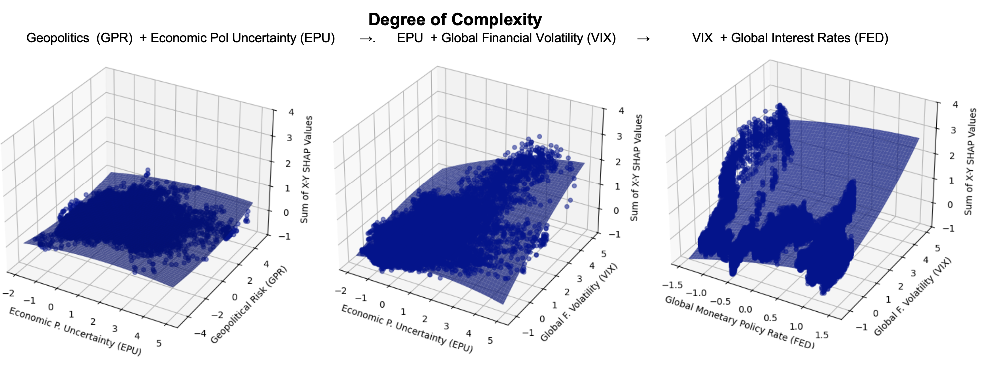
Notes: The figure illustrates the combined impact of key predictors on sovereign CDS spreads for Advanced Economies using two-factor SHAP dependence plots. The bottom row displays the joint influence of Geopolitical Risk (GPR) and Economic Policy Uncertainty (EPU). The middle row plots the joint contribution of EPU and Global Financial Volatility (VIX). The top row shows the joint effect of global financial volatility (VIX) and global monetary policy (FED).
The three scenarios and their results are as follows.
-
•
Scenario 1: Geoeconomics and policy uncertainty (GPR–EPU). This baseline scenario isolates the combined impact of non-financial uncertainty (Baker et al., 2016; Caldara and Iacoviello, 2022). For most regions, the joint surface is nearly flat, indicating low sensitivity to GPR and EPU when financial conditions are not controlled for. The exceptions are MENA—where structural geopolitical tensions steepen the surface—and, to a lesser extent, Emerging Europe.
-
•
Scenario 2: Uncertainty and financial volatility (EPU–VIX). Adding VIX to the picture produces a qualitative shift. The surface steepens markedly: high economic policy uncertainty in a high-VIX environment is substantially more detrimental than either shock alone, consistent with theories positing that uncertainty effects are magnified under financial stress (Bloom, 2009).
-
•
Scenario 3: Global financial conditions (VIX–FED). A simultaneous spike in global volatility and a tightening of monetary policy generates the largest and most nonlinear increases in sovereign risk. The surface also reveals an asymmetry: the impact of a volatility shock can be partially contained when interest rates remain low, but this mitigating effect is weaker than the amplification that occurs when both factors rise in tandem. The response to volatility is powerfully amplified when monetary policy is tight (Rey, 2013; Miranda-Agrippino and Rey, 2020) and partially contained when policy is accommodative, for instance through the risk-taking channel (Bruno and Shin, 2015; Bekaert et al., 2013).
The progression across scenarios confirms a critical transmission mechanism: geoeconomic or policy uncertainty, while often manageable in isolation, becomes a potent threat when it coincides with elevated global volatility and tighter financial conditions. This interaction between the financial and uncertainty blocks is paramount in determining sovereign vulnerability and motivates the cross-country interconnectedness analysis in the next subsection.
4.5 Interconnectedness and Spillovers
The preceding subsections characterize how global and domestic drivers shape sovereign risk within each country. We now shift perspective to examine how sovereign-risk attributions co-move and propagate across countries. We construct two complementary interconnectedness measures from the daily, country-level Shapley-implied risk series. First, a Diebold–Yilmaz (DY) dynamic spillover index based on rolling VARs summarizes the extent of directional, lagged transmission. Second, a non-parametric weighted network-density index from thresholded Spearman correlations captures contemporaneous clustering. Full details on rolling-window construction, VAR estimation, lag selection, generalized forecast-error variance decomposition (GFEVD) normalisation, and density computation are provided in Appendix D.
The two measures map distinct propagation mechanisms. High DY spillovers indicate multi-country transmission through lagged channels; high density reflects synchronous co-movement driven by common shocks. Episodes where both rise simultaneously correspond to systemic stress and broad-based repricing. Conversely, high density but low spillovers denotes localised synchronization without contagion, whereas high spillovers alongside low density indicates directional but unsynchronised propagation.
Figure 5 displays both indices—the DY total spillover (blue) and weighted network density (orange)—from 2021 onward, with vertical markers for the Russia–Ukraine invasion (February 2022), the Hamas–Israel conflict (October 2023), and the 2024 U.S. election. Equalised vertical scales permit direct comparison across variables. Three patterns emerge:
(Diebold–Yilmaz Spillovers and Network Density, 2021–2025)
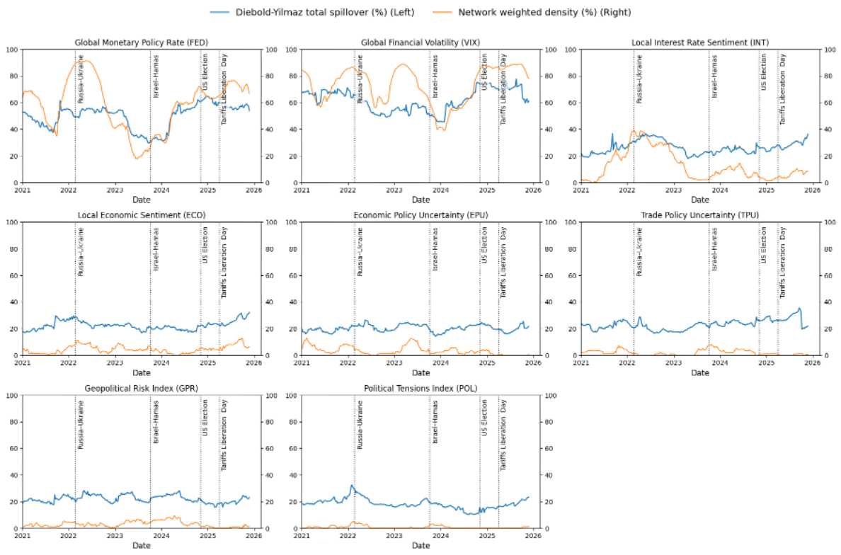
Notes: The figure reports dynamic spillover effects (blue line) and network density (orange line) for sovereign-risk determinants. Top row: global financial drivers (2-year UST, VIX, local interest rate sentiment). Middle row: local economic sentiment and uncertainty indices (EPU, TPU). Bottom row: geopolitical risk (GPR) and political tensions (POL). All indices are computed from daily, country-level Shapley attributions.
-
•
Global financial variables are the dominant and persistent transmitters. FED and VIX display the highest and most sustained DY values across the sample. Both spike sharply in early 2022, normalise through mid-2023, and rise again into late 2024. Network density moves closely with DY, consistent with system-wide repricing rather than localised contagion.
-
•
Local macro sentiment transmits directionally but with limited persistence. Local interest rate sentiment (INT) shows pronounced DY increases in 2022, coinciding with the global tightening–volatility shock, but density remains subdued thereafter—moderate DY with low density indicates directional propagation through monetary channels without broad synchronization. Local economic sentiment (ECO) displays a gradual DY rise into 2024–2025, but density remains intermittent, pointing to slow diffusion rather than unified contagion.
-
•
Geopolitical and policy-uncertainty shocks are episodic and synchronous. GPR and POL generate short, sharp density spikes around October 2023 (Hamas–Israel), while DY remains muted—an archetypal “common news” shock. EPU and, intermittently, TPU show similar brief increases. By late 2024, however, EPU displays rising density and DY, indicative of a broader policy-uncertainty cycle around the U.S. election rather than a region-specific disturbance. TPU remains consistently secondary, with only isolated upticks.
The dual-metric evidence establishes a clear hierarchy of cross-country transmission. Episodes with simultaneously high density and high DY—such as the early-2022 surge in global rates and volatility around the Russia–Ukraine invasion—reflect systemic stress, when shocks both synchronise markets and propagate dynamically across borders. High density with low DY, exemplified by the October 2023 Hamas–Israel conflict, captures common news events that trigger widespread repricing without durable contagion. Moderate DY with low density, observed as policy uncertainty rose ahead of the 2024 U.S. election, corresponds to directional spillovers through policy channels without full synchronization. The overarching implication is that global financial shocks set the systemic baseline of interconnectedness; geopolitical and policy-related uncertainty, while capable of generating sharp co-movements, act as episodic amplifiers whose effects dissipate unless reinforced by financial tightening.
5 Crisis Episodes: Geopolitical and Geoeconomic Uncertainty Shocks
We use the Shapley decomposition to trace transmission channels through three episodes that differ in scope and mechanism: an interstate war (Russia–Ukraine), a localized conflict (Hamas–Israel), and a geoeconomic uncertainty shock (U.S. new tariffs after US Presidential Election). In each case, we feed realized data through the estimated model—held fixed at its pre-episode parameters—and track daily Shapley contributions for the relevant countries. By virtue of local accuracy and consistency, the decomposition partitions day-by-day changes in predicted sovereign risk into additive driver contributions, enabling direct comparison across episodes.
5.1 Russia–Ukraine: From Regional Conflict to Systemic Stress
The February 2022 invasion illustrates how a geopolitical shock can cascade into systemic macro-financial stress. Figure 6 shows that CDS spreads for Russia and Ukraine spiked immediately, driven by surging GPR alongside rapid deterioration in domestic conditions. Sanctions and market exclusion magnified these pressures for Russia; for Ukraine, geopolitical premia combined with heightened policy uncertainty and collapsing domestic sentiment (Caldara and Iacoviello, 2022; Boubaker et al., 2023).

Notes: The figure plots the evolution of Shapley contributions to sovereign CDS spreads for selected countries before and after February 2022. For Russia and Ukraine, contributions from global monetary policy rates, global financial volatility, and geopolitical risk measures surge. For European economies, the impact is more moderate, with local sentiment and policy uncertainty amplifying exposure. Global financial conditions remain the dominant explanatory factor, while geopolitical tensions add substantial power for directly exposed countries.
The more consequential dynamic, however, unfolds in the months that follow. Among European neighbors, GPR contributions rise broadly but moderately. The initial geopolitical impulse is soon accompanied by a deterioration in local economic conditions: energy-driven inflation spikes feed through to domestic interest rates, adding a local-fundamentals channel to the Shapley attributions. The dominant shift, however, is the swift deterioration first in global policy rates and then in global financial volatility, as major central banks pivoted from accommodation to tightening roughly three months after the invasion. Energy dependence and supply-chain disruptions amplified the inflation impulse, transforming the geopolitical shock into a broader geoeconomic uncertainty episode once monetary policy reacted at both the local and global levels (Novta and Pugacheva, 2021; Lane, 2024). The attribution cascade reads:
In terms of our interconnectedness measures, this episode exhibits both high network density and high spillovers—a textbook case in which a regional conflict becomes systemic once it interacts with the global financial cycle (Bloom, 2009; Rey, 2013; Aiyar et al., 2023).
5.2 Hamas–Israel: Contained Shock under Benign Financial Conditions
The October 2023 Hamas–Israel conflict offers a contrasting pattern. For Israel, the Shapley decomposition shows an immediate and persistent increase in sovereign risk driven by GPR and deteriorating domestic conditions (Figure 7), consistent with direct conflict-risk pricing (Caldara and Iacoviello, 2022). Neighboring economies (Qatar, Turkey) registered muted GPR increases; for most other emerging markets and major Asian economies, geopolitical contributions remained essentially flat.

Notes: The figure plots the evolution of Shapley contributions to sovereign CDS spreads for selected countries before and after October 2023. For Israel, GPR and domestic condition contributions surge. For neighboring economies (Qatar, Turkey), increases are muted. For most other emerging markets and Asian economies, geopolitical contributions remain essentially flat, underscoring the contained nature of the shock.
The critical difference relative to Russia–Ukraine lies in the global financial backdrop acting as shock absorber. By October 2023, the Federal Reserve had held rates at 5.25–5.50 percent since July and signaled that the tightening cycle was likely at its peak (Board of Governors of the Federal Reserve, 2023b, a). As policy-rate expectations softened and volatility receded, global financial conditions shifted from amplifying to absorbing sovereign risk, offsetting contagion outside the immediate region. In our network metrics, this translates into high density but low spillovers: a common news shock largely contained by a benign global financial environment (Rey, 2013).
5.3 U.S. Election and Tariffs: Geoeconomic Uncertainty with Dual Transmission
The 2024 U.S. presidential election and subsequent tariff measures constitute a geoeconomic uncertainty shock—measured through EPU and TPU—with two distinct phases. Figure 8 shows that the election initially triggers spikes in EPU and TPU contributions for the United States and key trading partners (Canada, Mexico, China), reflecting heightened policy unpredictability. For most other emerging markets, immediate effects are muted and channeled primarily through global uncertainty.
With tariff implementation—culminating in “Liberation Day” (April 2, 2025)—uncertainty crystallizes into concrete trade barriers.

Notes: The figure shows Shapley contribution dynamics around the 2024 U.S. election and subsequent tariff announcements. For the United States, sovereign risk increases after the election and accelerates with tariff measures, driven by TPU, EPU, and global volatility. Spillovers are evident in Mexico, Canada, China, and Brazil through trade and policy uncertainty. For other economies, global financial drivers remain central, with uncertainty effects rising around tariff dates.
EPU and TPU contributions become the dominant drivers for directly exposed sovereigns, consistent with evidence that protectionism destabilizes credit premia (Ahn and Ludema, 2020; Itskhoki and Ribakova, 2024). For indirectly affected economies (Poland, Turkey, Brazil, Vietnam), the transmission operates differently: tariffs raise global volatility and shift monetary-policy expectations, transmitting risk through the global financial channel rather than direct trade exposure (Glick and Rose, 1999; Diebold and Yilmaz, 2012). This dual mechanism—direct trade exposure for core participants, global financial amplification for the rest—exemplifies a geoeconomic uncertainty scenario in which economic and trade policy uncertainty and the global financial cycle interact nonlinearly, reinforcing the patterns documented in the SHAP dependence analysis.
5.4 Comparing the Three Episodes
The three cases reveal systematic differences in shock type, transmission, and interaction with the global financial cycle:
-
•
Nature of the shock. Russia–Ukraine and Hamas–Israel are geopolitical shocks dominated by GPR, with domestic conditions deteriorating for directly affected sovereigns (Gorodnichenko et al., 2025).171717Gorodnichenko et al. (2025) document that higher perceived conflict durations raise expectations of stagflation, worsen views on public finances, and depress consumption. The tariff episode is a geoeconomic uncertainty shock driven by EPU and TPU.
-
•
Epicenter versus periphery. Conflict participants (Russia, Ukraine, Israel) suffer persistent sovereign-risk repricing through geopolitical shock but also deteriorating local fundamentals. For non-epicenter countries, the impact depends on whether the shock morphs into a systemic episode—as Russia–Ukraine did via commodity markets and inflation—or remains contained, as Hamas–Israel did under benign global conditions.
-
•
Primary transmission channel. Russia–Ukraine propagated via proximity, energy dependence, and inflation into global financial tightening. Hamas–Israel remained regional, with the global financial cycle acting as absorber. The tariff episode operated through a direct trade channel for core participants and through the global financial channel for the rest.
-
•
State-dependent role of the global financial cycle. The GFC amplified Russia–Ukraine (tightening compounded the geopolitical impulse), absorbed Hamas–Israel (easing contained spillovers), and propagated tariff effects (geoeconomic uncertainty itself triggered tighter global conditions). Whether a shock becomes systemic depends less on its origin than on its interaction with global monetary and volatility conditions (Rey, 2013; Bloom, 2009).
Overall, the narrative evidence reinforces the model-based findings: global financial factors dominate Shapley contributions and network spillovers, while geopolitical and geoeconomic uncertainty shocks matter most when they coincide with tight and volatile global conditions, reinforcing the nonlinear patterns documented in Section 4.
6 A Taxonomy of Shock Transmission
Recall from Section 3 that the Shapley–Taylor decomposition (equation 3) partitions the total contribution of any driver to the predicted sovereign CDS spread into four mutually exclusive channels by grouping its pairwise interactions according to the economic block of the partner variable. The decomposition is exact and can be grouped in these channels at every observation by the local accuracy property of Shapley values Shapley (1953) and the extension on Taylor Shap Lundberg and Lee (2017):
Figure 9 and Table 2 apply this framework to four episodes that span the geopolitical–geoeconomic spectrum. The Own Direct Effect () measures how much the shock reprices sovereign default probability on its own. The Global Financial Conditions channel () captures how the shock’s effect is amplified or absorbed by the U.S. monetary policy and global volatility (). The Uncertainty channel () measures cross-reinforcement with economic and trade-policy uncertainty (). The Local & Political Conditions channel () captures how domestic economic sentiment, interest-rate expectations, and political tensions interact with the external shock (). The question is whether geopolitical and geoeconomic uncertainty shocks use these channels differently—and they do, in three ways: they enter through different channels, they hit countries differently depending on global financial exposure and domestic conditions, and they fade at different speeds.

Notes: Each panel plots the cross-sectional average (42 countries) of the four Shapley–Taylor transmission channels (equation 3) for the indicator most directly associated with each episode: GPR for Russia–Ukraine (a) and Hamas–Israel (b), EPU for the Trump Election (c), and TPU for the U.S. tariff shock (d). Own Direct Effect (red): own Shapley–Taylor term . Global Financial Conditions (blue): interactions with VIX and FED. Uncertainty (orange): interactions with EPU and TPU. Local & Political Conditions (green): interactions with ECO, INT, and POL. Dotted black line: total Shapley contribution. Vertical dashed lines mark the event date. All series are 28-day moving averages.
Geopolitical and geoeconomic shocks enter through different doors.
The four panels of Figure 9 make the distinction visible. In panel (a), the Russia–Ukraine invasion opens a “scissors”: the Direct channel (red) jumps to roughly within days as conflict exposure reprices default probability (Caldara and Iacoviello, 2022), while the GFC (blue) plunges symmetrically to approximately as the global financial system partially absorbs the shock through the risk-taking channel (Rey, 2013; Bruno and Shin, 2015). The two move in mirror image—a “flight to safety” in which risky and safe exposures reprice simultaneously in opposite directions (Baele et al., 2020)—so the total (dotted black) rises only modestly despite large individual movements. The Local channel (green) drifts upward more gradually in subsequent weeks; the Uncertainty channel (orange) remains flat. Crucially, the scissors stay open through July 2022—neither channel returns to its pre-event level.
Panel (b) shows a similar but muted pattern for Hamas–Israel. The Direct channel spikes, but the GFC response is far smaller—a first indication that a regional conflict does not disrupt the global financial cycle as severely as a systemic one. The Local channel, by contrast, rises in parallel with the Direct channel and persists through February 2024, foreshadowing the result below that domestic amplifiers matter more in this episode.
The geoeconomic episodes invert the picture entirely. In panel (c), the Direct channel is flat throughout—the U.S. election does not reprice default probability. Instead, the GFC begins declining three months before the November 2024 event as markets price in looser monetary policy (Miranda-Agrippino and Rey, 2020), and continues falling to roughly by December. The total is driven almost entirely by the red line; the blue line barely moves. Panel (d) is the most dramatic: the GFC plunges from near zero to approximately within two weeks of the April 2025 tariff announcement, then partially recovers. Once again, the Direct channel stays at zero—the tariff shock shifts expected monetary policy and risk appetite, not default probability—while the Local channel ticks up modestly, consistent with the originator premium documented below.
Table 2 confirms these visual patterns with precise magnitudes. The Direct channel dominates the GFC at the panel level in both geopolitical episodes ( vs. for Russia–Ukraine; vs. for Hamas–Israel); the GFC dominates the Direct channel in both geoeconomic episodes. The organising principle is clear: geopolitical shocks reprice default risk directly and provoke an offsetting financial-system response; geoeconomic shocks bypass default risk entirely and operate through the financial system.
The same shock hits countries differently, depending on global financial exposure and domestic conditions.
Why does the Russia–Ukraine war devastate Ukrainian spreads but barely move Brazil’s? The answer lies in the relative weight of two forces. The first is the sovereign’s exposure to the global financial cycle—how integrated it is into dollar-funding markets, how sensitive to VIX and the Fed—which determines the size of . The second is the state of the sovereign’s own economy—domestic sentiment, interest-rate expectations, political stability—which determines the size of . These two forces operate through separate sets of covariates by construction: aggregates interactions with ; aggregates interactions with .
Table 2 reveals three distinct transmission modes within the geopolitical episodes alone. Ukraine is overwhelmingly a GFC story: , the largest single-channel value in the sample. Sanctions and market exclusion converted a geopolitical shock into a financial-intermediation event (Fernández-Villaverde et al., 2024). But the Local channel is also large (): the simultaneous collapse of domestic sentiment, the spike in interest-rate expectations, and political tensions compounded the effect through a separate mechanism. Israel presents a different balance: and —the two channels contribute almost equally, reflecting the joint activation of global risk-appetite sensitivity and domestic amplifiers (mobilisation costs, fiscal expansion, political fractures; Gorodnichenko et al., 2025). The contrast between for Israel and for Ukraine is economically meaningful: Ukraine’s crisis is primarily one of financial exclusion; Israel’s is equally a story of domestic strain. Poland illustrates a third mode—GFC compensation: the Direct-channel rise of is nearly offset by , because deep integration into European capital markets provides a built-in shock absorber.
The geoeconomic episodes reveal a further asymmetry. At the panel level, the tariff shock compresses spreads through the GFC as expected monetary easing benefits everyone. But the United States—the originator—is the exception. Its GFC contribution is a negligible , while its Local channel registers : the policy uncertainty the originator created raises its own fiscal and political-risk premia through the interaction of TPU with domestic sentiment, interest-rate expectations, and political tensions. The originator does not benefit from the monetary easing it provokes—a form of asymmetric transmission consistent with Forbes and Rigobon (2002) and with recent evidence that geoeconomic instruments generate domestic risk premia (Clayton et al., 2025). The result also confirms a theoretical prediction of Pástor and Veronesi (2013): policy uncertainty generates risk premia that are largest for the country whose government is the source of that uncertainty. More broadly, the originator’s inability to benefit from the global easing it triggers echoes the mechanism in Farhi and Maggiori (2018), in which the reserve-currency issuer can undermine its own privilege through fiscal indiscipline. The policy implication is direct: GFC-mediated widening can be addressed through central-bank swap lines and global liquidity provision (Bahaj and Reis, 2022); Local-channel widening cannot—it requires fiscal, institutional, or political adjustment at the country level.
The speed of decay reveals what each channel is made of.
If the Direct channel captures fundamental repricing and the GFC captures liquidity adjustments, they should fade at different speeds—and they do. The Direct channel retains roughly two-thirds of its one-month value at three months in both geopolitical episodes: the underlying conflicts remain unresolved, so the default-probability repricing persists (Caldara and Iacoviello, 2022; Boubaker et al., 2023). The GFC decays faster and can reverse sign entirely, because risk-appetite shocks are mean-reverting (Bekaert et al., 2013; Bloom, 2009). The Local channel sits in between.
| Short-Term Impact () | Persistence () | ||||||||||
| Nature of Shock | |||||||||||
| Panel A : Russia–Ukraine (GPR, Feb. 2022) | |||||||||||
| Panel avg. | Geopolitics (Panel A) | ||||||||||
| Ukraine | |||||||||||
| Poland | |||||||||||
| Germany | |||||||||||
| Panel B : Hamas–Israel (GPR, Oct. 2023) | |||||||||||
| Panel avg. | Geopolitics (Panel B) | ||||||||||
| Israel | |||||||||||
| Egypt | |||||||||||
| Germany | |||||||||||
| Panel C : Trump Election (EPU, Nov. 2024) | |||||||||||
| Panel avg. | Economic Uncertainty (Panel C) | ||||||||||
| USA | |||||||||||
| Mexico | |||||||||||
| Germany | |||||||||||
| Panel D : U.S. Tariffs / Liberation Day (TPU, Apr. 2025) | |||||||||||
| Panel avg. | Trade Uncertainty (Panel D) | ||||||||||
| USA | |||||||||||
| India | |||||||||||
| Germany | |||||||||||
Notes: Each cell reports (s.d. of standardized CDS spread). Short-Term Impact: post-window = 1 month after event onset. Persistence: post-window = 3 months after event onset. Pre-event window = 3 months in both cases. Cell shading: , , , , . Values in -CDS units. Panel avg. = unweighted cross-country mean (42 countries). Germany appears in all panels as a common benchmark. 28-day moving averages applied to all series.
Egypt makes this concrete. At impact, all four channels amplify: . By three months, the GFC has reversed () and the Local channel has followed (), dragging the total down to . What happened? The initial widening was driven by two transient forces—a global liquidity squeeze and a domestic sentiment shock—that mean-reverted as conditions normalized. But the Direct channel barely moved (): Egypt’s fundamental exposure to the conflict persisted even after the financial and domestic amplifiers faded. Mexico illustrates the opposite dynamic: its near-zero impact turns significantly negative at three months (), as the GFC and Local channels accumulated while trade-policy uncertainty materialized into actual tariff actions (Caldara et al., 2020).
Taxonomy belongs to the shock, not the country: Germany as a natural experiment.
Because Germany appears in all four panels, it offers a clean test: hold the country constant, change the shock, and see which channels activate. The answer is unambiguous. When the shock is geopolitical, Germany’s transmission is dominated by the Direct channel pulling spreads up and the GFC pulling them back down—a tug-of-war between conflict-driven repricing and the financial system’s absorption capacity ( against for Russia–Ukraine; against for Hamas–Israel). The Local and Uncertainty channels barely register. When the shock is geoeconomic, the pattern flips: the Direct channel goes silent, and transmission shifts entirely to the GFC ( for tariffs) and the Uncertainty channel ( for the election). Nothing about Germany’s economy changed between these episodes—its financial structure, its institutions, its trade openness are the same. What changed is the nature of the shock. The channel that carries the shock to sovereign spreads is therefore determined by what kind of shock it is, not by which country receives it—consistent with the state-dependent interaction surfaces in Figure 4.
In sum, geopolitical shocks reprice default probability directly and persistently, with the global financial system acting as a contemporaneous but transient stabiliser (Rey, 2013; Bruno and Shin, 2015). Geoeconomic shocks bypass the direct channel entirely, operating through expected monetary policy and risk appetite; they compress average spreads, with the originator as a notable exception (Clayton et al., 2025). That fundamental repricing endures while financial amplification reverts (Bekaert et al., 2013) provides an independent validation of the taxonomy—and implies that liquidity interventions can address GFC-mediated transmission but not the durable component of geopolitical risk premia.
6.1 The Geography of Geopolitical Risk Transmission
If geopolitical shocks reprice default probability in proportion to conflict exposure, then countries closer to the conflict should register larger Direct-channel effects—a gravity-style prediction familiar from the trade literature (Head and Mayer, 2014) and from early work linking geographic proximity to financial contagion (Glick and Rose, 1999). Figure 10 tests this by regressing the short-term direct effect on great-circle distance from each national capital to the conflict epicentre:
| (6) |
where is distance to Kyiv (left panel) or Tel Aviv (right panel).
The Russia–Ukraine shock produces a steep, monotonically declining gradient ( per 1,000 km and significant at 1% level; , ). Countries within 1,200 km of Kyiv—Czech Republic (), Germany (), Finland ()—are hit two to three times harder than the cross-sectional mean; Latin American and Asia-Pacific sovereigns converge toward zero beyond 10,000 km. Distance works as a summary statistic because it proxies for the constellation of trade, energy, and security linkages that connect European sovereigns to the conflict zone.
The Hamas–Israel shock reveals a different geography. The slope is roughly half as steep ( but significant (5% level); , ) and explanatory power is concentrated among MENA sovereigns within 2,000 km: Egypt (), Israel (), Qatar (). Beyond the regional perimeter the relationship flattens—except for the Philippines ( at 9,200 km), an outlier readily explained by diaspora-remittance exposure rather than geographic contiguity. This single case illustrates both the power and the limitation of the distance proxy: it organises the bulk of the cross section, but cannot capture transmission that runs through labour-market and financial channels orthogonal to geography.
The contrast between the two panels is itself informative. Systemic geopolitical shocks generate gravity-like decay well approximated by a single distance regressor; regionally contained conflicts produce steep local gradients that flatten globally, punctuated by outliers reflecting non-geographic bilateral exposures. That the Netherlands () and Indonesia () register mildly negative direct effects suggests that for a subset of sovereigns the geopolitical shock operates as a safe-haven event, consistent with portfolio-rebalancing channels documented in the contagion literature (Forbes and Rigobon, 2002) and with empirical evidence on safe-haven dynamics in sovereign markets (Habib and Stracca, 2012). The appendix tables document additional cross-sectional variation in the GFC and Local channels across the geoeconomic episodes; we leave formal analysis of those patterns to future work.
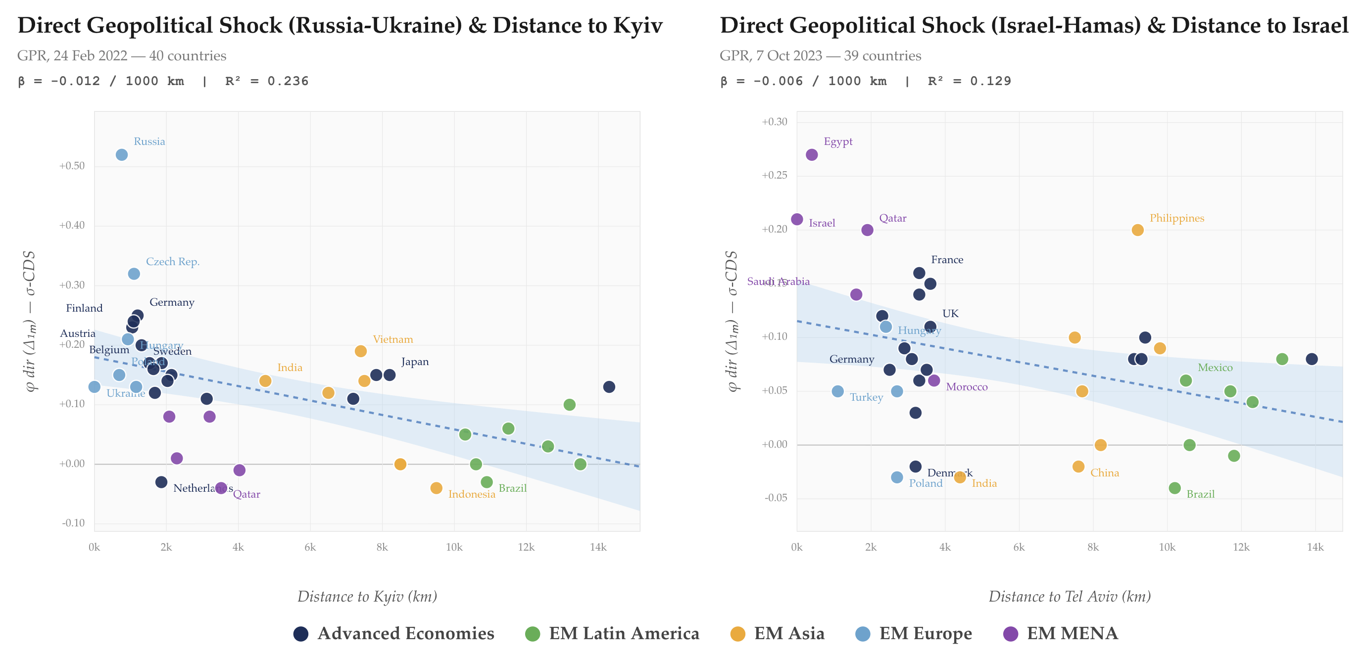
Notes: Each panel plots the Own Direct channel () against great-circle distance (km) from the national capital to the conflict epicentre (Kyiv, left panel; Tel Aviv, right panel). The decomposition follows equation (3). Left panel: 40 sovereigns (Russia–Ukraine, 24 February 2022). Right panel: 39 sovereigns (Hamas–Israel, 7 October 2023). Dashed lines: OLS fitted values from equation (6); shaded bands: 95% confidence intervals. The coefficient are significat at 1% (Russsia-Ukraine) and 5% (Hamas-Israel) levels. All values in within-country standard deviations of CDS spreads (-CDS). Jordan excluded due to insufficient pre-2023 CDS data.
6.2 The Fingerprint of Policy Uncertainty.
The election episode leaves a trace in the data that no other shock produces: the Uncertainty channel lights up for nearly every country in the sample simultaneously. At the panel level it registers at both horizons; the appendix tables confirm positive values for France, Brazil, China, Germany (), and most other sovereigns. This broad-based activation is absent from the other three episodes. In the tariff shock, is negligible—the shock operates through the GFC, not through uncertainty cross-reinforcement. In both geopolitical episodes, is near zero outside the conflict zone—the shock reprices default probability directly rather than raising global policy uncertainty. The pattern is consistent with models in which political uncertainty generates correlated risk premia across all assets simultaneously (Pástor and Veronesi, 2012; Baker et al., 2016): when the source of uncertainty is a major election rather than a war or a tariff, every sovereign’s spread is affected through the same uncertainty channel at once.
This result completes a three-way fingerprint. Geopolitical shocks activate with gravity-like cross-sectional structure. Trade shocks operate through in proportion to bilateral exposure. Policy-uncertainty shocks activate globally. Each shock type has a distinct first-responder channel and a distinct cross-sectional distribution—so a monitoring authority observing which channel fires first can classify the shock before its macroeconomic effects materialize.
7 Conclusion
The central finding of this paper is that geopolitical and geoeconomic shocks propagate to sovereign spreads through qualitatively distinct mechanisms—and that these mechanisms can be formally separated. A four-channel Shapley–Taylor decomposition that partitions each observation’s predicted spread into Direct, Global Financial Cycle (GFC), Uncertainty, and Local Macro-Political channels reveals a clean structural taxonomy. Geopolitical episodes exhibit a “scissors” pattern in which the Direct channel rises sharply on impact—repricing default probability—while the GFC falls, as the global financial system partially absorbs the shock. Geoeconomic episodes invert this pattern entirely: the Direct channel is inert and spreads respond almost exclusively through the GFC, as markets reprice expected monetary policy and risk appetite. These channels also differ in persistence: fundamental repricing endures because the underlying conflict remains unresolved, whereas financial amplification mean-reverts. This differential persistence provides independent validation of the taxonomy. At the country level, the same channel activation pattern holds, with financial integration determining which channel dominates and geoeconomic originators facing an asymmetric penalty as the domestic Local channel widens their own spreads even as they compress spreads abroad.
Each shock type leaves a distinct cross-sectional fingerprint. Geopolitical Direct effects decay with geographic distance from the conflict zone. Trade-policy shocks propagate through the GFC, with transmission shaped by bilateral trade exposure and financial integration. Policy-uncertainty shocks activate the Uncertainty channel globally and simultaneously—a pattern absent from all other episode types. Together, these signatures allow a monitoring authority to classify the nature of a shock before its macroeconomic consequences materialize.
Two features of the empirical design merit emphasis. First, nonlinear machine-learning models are better equipped to capture inherently nonlinear events such as geopolitical shocks and tariff escalations, and our forecasting horse race confirms that news-based indicators add predictive value primarily when embedded in nonlinear specifications. Second, our two-stage architecture explicitly separates advanced-economy sovereign debt—which often trades as a safe asset—from riskier emerging-market credit, and the channel decomposition documents pronounced heterogeneity across these asset classes and regions, with geopolitical risk most salient in Emerging Europe and MENA and global financial conditions dominant elsewhere.
For policymakers, the taxonomy carries concrete operational content: GFC-mediated spread widening is addressable through central-bank swap lines and liquidity provision, whereas direct default-probability repricing requires diplomatic resolution or fiscal and institutional adjustment. Monitoring high-frequency text-based indicators can provide timely warnings when uncertainty or geopolitical risks begin to amplify the effects of global tightening.
Several limitations warrant acknowledgment. The Shapley–Taylor decomposition attributes model predictions, not structural causal effects, though we mitigate known limitations of standard Shapley values—notably their inability to capture interactions—by adopting Shapley–Taylor interaction indices that exactly decompose predictions into own effects and pairwise terms, enabling the channel grouping at the core of our taxonomy. Despite its interpretive nature, the framework displays strong internal coherence: the same taxonomy emerges across four distinct episodes, channel signatures align with economic theory, and differential channel persistence is consistent with the structural content each captures.
Whether the taxonomy extends to other maturities, currencies, or non-sovereign markets remains an open question. A natural next step is to embed the four-channel framework into structural models of sovereign risk and capital allocation and to examine whether the shock-type fingerprint retains its discriminating power in real-time monitoring applications.
References
- A new era of global financial vulnerability. Note: Global Financial Stability Report, International Monetary Fund Cited by: footnote 16.
- The world uncertainty index. Brookings Papers on Economic Activity, pp. 343–400. Cited by: §1, 2nd item.
- The sword and the shield: the economics of targeted sanctions. European Economic Review 130, pp. 103578. External Links: Document Cited by: §1, §5.3.
- Geoeconomic fragmentation and the future of multilateralism. Staff Discussion Note Technical Report SDN/2023/001, International Monetary Fund. Cited by: §1, §5.1.
- Rethinking GPR: the sources of geopolitical risk. Documentos de Trabajo Technical Report 2522, Banco de España. Cited by: §1, §2, footnote 5.
- The dynamics of spillover effects during the European sovereign debt turmoil. Journal of Banking & Finance 42, pp. 134–153. Cited by: §3.4.
- Machine learning methods that economists should know about. Annual Review of Economics 11, pp. 685–725. Cited by: §4.1.
- The impact of machine learning on economics. In The Economics of Artificial Intelligence: An Agenda, pp. 507–547. Cited by: §1.
- Flights to safety. Review of Financial Studies 33 (2), pp. 689–746. Cited by: §6.
- Central banking in challenging times: central bank liquidity lines. American Economic Journal: Macroeconomics 14 (2), pp. 110–150. Cited by: §1, §1, 1st item, §6.
- Measuring economic policy uncertainty. Quarterly Journal of Economics 131 (4), pp. 1593–1636. Cited by: §1, §1, §2, §3.3, 3rd item, 1st item, §4.1, §6.2.
- BIS annual economic report 2022. Technical report Bank for International Settlements. Cited by: §1.
- Network science. Cambridge University Press, Cambridge. Cited by: §3.4.
- Flight-to-quality—money market mutual funds and stablecoins during the March 2023 banking crisis. Economics Letters 234, pp. 111464. Cited by: 2nd item.
- Risk, uncertainty and monetary policy. Journal of Monetary Economics 60 (7), pp. 771–788. Cited by: §1, 3rd item, §6, §6.
- Sanctions and Russian online prices. Journal of Economic Behavior & Organization 225, pp. 483–521. Cited by: §1.
- Really uncertain business cycles. Econometrica 86 (3), pp. 1031–1065. Cited by: §1.
- The impact of uncertainty shocks. Econometrica 77 (3), pp. 623–685. Cited by: §3.3, §3.3, 2nd item, 4th item, §5.1, §6.
- Systemic risk and financial spillovers: a machine learning approach. Journal of Monetary Economics 134, pp. 80–99. Cited by: §1, §4.1.
- Minutes of the federal open market committee, september 2023. Note: Washington, DC Cited by: §5.2.
- Monetary policy report. Note: Washington, DC Cited by: §5.2.
- Geopolitical risk perceptions. Journal of International Economics 152, pp. 104005. Cited by: §1, §2, footnote 5.
- Geopolitical risk and energy stock performance: evidence from the Russia–Ukraine conflict. Journal of Commodity Markets 30, pp. 100325. Cited by: §1, §1, §5.1, §6.
- Random forests. Machine Learning 45 (1), pp. 5–32. Cited by: §3.1, footnote 14.
- Reversal of capital flows and emerging market vulnerability. Journal of Monetary Economics 85, pp. 28–44. Cited by: 3rd item.
- Capital flows and the risk-taking channel of monetary policy. Journal of Monetary Economics 71, pp. 119–132. Cited by: 3rd item, §6, §6.
- Economic policy uncertainty spillovers in booms and busts. Journal of Monetary Economics 115, pp. 735–751. External Links: Document Cited by: 2nd item.
- The economic effects of trade policy uncertainty. Journal of Monetary Economics 109, pp. 38–59. Cited by: §1, §1, §3.3, 3rd item, §6.
- Measuring geopolitical risk. American Economic Review 112 (4), pp. 1194–1225. Cited by: §1, §1, 2nd item, 1st item, §4.1, §5.1, §5.2, §6, §6.
- On the empirics of sudden stops: the relevance of balance-sheet effects. Working Paper Technical Report 10520, National Bureau of Economic Research. Cited by: §1.
- Inflows of capital to developing countries in the 1990s. Journal of Economic Perspectives 10 (2), pp. 123–139. Cited by: §1, §3.2.
- Geoeconomic pressure. Working Paper Technical Report 34020, National Bureau of Economic Research. Cited by: §1, §1, §6, §6.
- Empirical properties of asset returns: stylized facts and statistical issues. Quantitative Finance 1 (2), pp. 223–236. Cited by: §1.
- Macro shocks and firm-level response heterogeneity. Working Paper Technical Report 33929, National Bureau of Economic Research. Cited by: §1.
- The economic impact of conflict-related and policy uncertainty shocks: the case of Russia. International Economics 174, pp. 69–90. Cited by: §1.
- The information content of conflict, social unrest and policy uncertainty measures for macroeconomic forecasting. Latin American Journal of Central Banking 5 (4), pp. 100130. Cited by: §1.
- Financial globalization in emerging economies: much ado about nothing?. Journal of Development Economics 98 (1), pp. 86–104. Cited by: §1.
- Better to give than to receive: predictive directional measurement of volatility spillovers. International Journal of Forecasting 28 (1), pp. 57–66. Cited by: §5.3.
- On the network topology of variance decompositions: measuring the connectedness of financial firms. Journal of Econometrics 182 (1), pp. 119–134. Cited by: B.2. Generalized Forecast-Error Variance Decomposition, §1, §3.4, §3.
- The dollar, bank funding and global financial conditions. Journal of Finance 73 (2), pp. 537–586. Cited by: §1, 1st item.
- Original sin redux: a modern assessment of emerging-market vulnerabilities. Journal of International Money and Finance 110, pp. 102280. Cited by: 2nd item.
- European central bank working paper no. 2973. Technical report European Central Bank. Cited by: footnote 16.
- A model of the international monetary system. Quarterly Journal of Economics 133 (1), pp. 295–355. Cited by: §1, §6.
- Commodity price synchronicity and financial variables. Journal of International Financial Markets, Institutions and Money 56, pp. 26–40. Cited by: §1.
- Charting the uncharted: the (un)intended consequences of oil sanctions and dark shipping. Working Paper Technical Report 33486, National Bureau of Economic Research. Cited by: §1.
- Are we fragmented yet? measuring geopolitical fragmentation and its causal effects. Working Paper Technical Report 32638, National Bureau of Economic Research. Cited by: §1, §6.
- No contagion, only interdependence: measuring stock market comovements. Journal of Finance 57 (5), pp. 2223–2261. Cited by: §6, §6.1.
- Capital flows, push versus pull factors and the global financial crisis. Journal of International Economics 88 (2), pp. 341–356. Cited by: §1, §3.2.
- Greedy function approximation: a gradient boosting machine. Annals of Statistics 29 (5), pp. 1189–1232. Cited by: §3.1.
- Regional economic outlook: middle east and central asia. Note: Washington, DC Cited by: 2nd item.
- Sovereign borrowing by developing countries: what determines the bond spread?. Journal of Development Economics 96 (2), pp. 273–282. Cited by: 1st item.
- Text as data. Journal of Economic Literature 57 (3), pp. 535–574. Cited by: §1, §4.1.
- Contagion and trade: why are currency crises regional?. Journal of International Money and Finance 18 (4), pp. 603–617. Cited by: §1, §5.3, §6.1.
- Banking globalization, monetary transmission, and the global financial cycle. Journal of International Economics 125, pp. 103–118. Cited by: §1, 1st item.
- The impact of geopolitical risk on consumer expectations and spending. Working Paper Technical Report 34195, National Bureau of Economic Research. Cited by: 1st item, §6, footnote 17.
- How is machine learning useful for macroeconomic forecasting?. Journal of Applied Econometrics 37 (5), pp. 920–964. Cited by: §4.1.
- Empirical asset pricing via machine learning. Review of Financial Studies 33 (5), pp. 2223–2273. Cited by: §1, §4.1.
- Getting beyond carry trade: what makes a safe haven currency?. Journal of International Economics 87 (1), pp. 50–64. Cited by: §6.1.
- Bank networks and cross-border financial transmission. Journal of International Economics 124, pp. 103127. Cited by: 3rd item.
- A new approach to the economic analysis of nonstationary time series and the business cycle. Econometrica 57 (2), pp. 357–384. Cited by: §1.
- Firm-level political risk: measurement and effects. Quarterly Journal of Economics 134 (4), pp. 2135–2202. Cited by: §1.
- Gravity equations: workhorse, toolkit, and cookbook. In Handbook of International Economics, G. Gopinath, E. Helpman, and K. Rogoff (Eds.), Vol. 4, pp. 131–195. Cited by: §1, §6.1.
- Ridge regression: biased estimation for nonorthogonal problems. Technometrics 12 (1), pp. 55–67. Cited by: §3.1.
- Global financial stability report. Technical report International Monetary Fund. Cited by: §1.
- Global financial stability report. Note: April 2023, Washington, DC Cited by: 2nd item.
- The economics of sanctions: from theory into practice. Technical report Brookings Institution. Note: Brookings Papers on Economic Activity Conference Draft Cited by: §5.3.
- Machine learning for financial crises prediction: an empirical comparison with linear models. Journal of Financial Stability 56, pp. 100939. Cited by: §1.
- European central bank monetary policy and the inflation surge. European Central Bank Economic Bulletin. Cited by: §5.1.
- Deep learning. Nature 521 (7553), pp. 436–444. Cited by: §3.1.
- GDELT: global data on events, location, and tone, 1979–2012. Technical Report Technical Report Version 1.0, GDELT Project. Note: Presented at the International Studies Association Annual Convention, San Francisco, CA Cited by: §2.
- A unified approach to interpreting model predictions. In Advances in Neural Information Processing Systems, Vol. 30, pp. 4765–4774. Cited by: §1, §3.3, §3, §4.4, §6.
- International currencies and capital allocation. Journal of Political Economy 128 (6), pp. 2019–2066. Cited by: §1.
- News implied volatility and disaster concerns. Journal of Financial Economics 123 (1), pp. 137–162. Cited by: §1.
- U.S. monetary policy and the global financial cycle. Review of Economic Studies 87 (6), pp. 2754–2776. Cited by: §1, §3.2, §3.3, 1st item, 3rd item, §6.
- Reading between the lines: prediction of political violence using newspaper text. American Political Science Review 112 (2), pp. 358–375. Cited by: §1.
- Using past violence and current news to predict changes in violence. International Interactions 48 (4), pp. 579–596. Cited by: §1.
- Machine learning: an applied econometric approach. Journal of Economic Perspectives 31 (2), pp. 87–106. Cited by: §1, §3.1, §3, §4.1.
- Networks: an introduction. Oxford University Press, Oxford. Cited by: §3.4.
- Geopolitical risks and capital flows to emerging markets. Journal of International Money and Finance 115, pp. 102391. Cited by: §1, §1, §5.1.
- Uncertainty about government policy and stock prices. Journal of Finance 67 (4), pp. 1219–1264. Cited by: §1, §6.2.
- Political uncertainty and risk premia. Journal of Political Economy 121 (1), pp. 36–72. Cited by: §1, §6.
- Inequality aversion, populism, and the backlash against globalization. Journal of Finance 76 (6), pp. 2857–2906. External Links: Document Cited by: 2nd item.
- Generalized impulse response analysis in linear multivariate models. Economics Letters 58 (1), pp. 17–29. Cited by: B.2. Generalized Forecast-Error Variance Decomposition.
- Debt intolerance. Brookings Papers on Economic Activity 2003 (1), pp. 1–74. Cited by: §1.
- Dilemma not trilemma: the global financial cycle and monetary policy independence. In Proceedings of the Jackson Hole Economic Policy Symposium, pp. 285–333. Cited by: §1, §3.2, §3.3, 1st item, 3rd item, 4th item, §5.1, §5.2, §6, §6.
- A value for -person games. In Contributions to the Theory of Games, Vol. 2, pp. 307–317. Cited by: §1, §3.3, §6.
- Measuring the effects of federal reserve forward guidance and asset purchases on financial markets. Journal of Monetary Economics 118, pp. 32–53. Cited by: 1st item.
- Specification, estimation, and evaluation of smooth transition autoregressive models. Journal of the American Statistical Association 89 (425), pp. 208–218. Cited by: §1.
- Regression shrinkage and selection via the lasso. Journal of the Royal Statistical Society: Series B (Methodological) 58 (1), pp. 267–288. Cited by: §3.1.
- Big data: new tricks for econometrics. Journal of Economic Perspectives 28 (2), pp. 3–28. Cited by: §1, §3.1, §4.1.
- Regularization and variable selection via the elastic net. Journal of the Royal Statistical Society: Series B (Statistical Methodology) 67 (2), pp. 301–320. Cited by: §3.1.
Appendix A APPENDIX A: The data
This annex details country-specific data availability, as well as percentile distributions by country (Appendix A.1), as well as the procedures employed for the construction of the news-based indicators used in the empirical analysis (Appendix A.2).
A.1 Data availability by country
We include a summary describing the basis for the empirical analysis developed in the paper. The following table presents country-specific data availability together with descriptive statistics summarizing the distribution of the main variables. For each country, the start and end dates of the available sample are reported. To characterize the distribution, we provide the 25th and 75th percentiles (p25 and p75), which capture the inter-quartile range where the central 50% of observations lie, for each of the described variables in the data section.
![[Uncaptioned image]](2510.12416v5/Graphs/data_table.png)
A.2 Media sentiment indicators development process
All indices are developed by BBVA Research using the Global Database of Events, Language, and Tone (GDELT) as described previously in the data section. The indices are daily and collected at the country level. To ensure homogeneity, each index is normalized (minus average and divided by standard deviation) and smoothed using a 28-day moving average. This transformation reduces daily noise and allows for a clearer identification of signals. No outlier treatment is performed, since the objective is to capture events that stand out from the normal behavior of the indicators.
The detailed set of keywors included in each case to build the indicators are the following:
-
•
Economic Policy Uncertainty (EPU) Index
The Economic Policy Uncertainty (EPU) Index is originally constructed by BBVA Research based on the relative coverage associated with GDELT searches using country-specific keywords. The specific choice of keywords for each country aims to replicate the methodology presented by Baker, Bloom and Davis (2016) in “Measuring Economic Policy Uncertainty”.
-
–
United States: “United States (uncertainty OR uncertain) (economic OR economy) (congress OR legislation OR white house OR regulation OR federal reserve OR deficit)"
-
–
China: "China (uncertain OR uncertainty) (economy OR economic OR business) (fiscal OR monetary OR Commission OR bank OR legislation OR tax OR bonds OR debt OR tariff OR deficit)"
-
–
Canada: "Canada (uncertain OR uncertainty)(economic OR economy)(policy OR tax OR spending OR regulation OR central bank OR budget OR deficit)"
-
–
Mexico: "Mexico (economic OR economy) (uncertain OR uncertainty) (regulation OR deficit OR budget OR Bank OR BdeM OR Banxico OR congress OR senate OR deputies OR legislation OR taxes OR Federal Reserve)"
-
–
Spain: "Spain (uncertainty OR uncertain OR instability OR risk) (economic OR economy) (parliament OR government OR Hacienda OR deficit OR budget OR expenditure OR debt OR taxes OR law OR reform OR regulation OR Bank)"
-
–
Australia: "Australia (uncertain OR uncertainty) (economic OR economy) (regulation OR Reserve Bank of Australia OR RBA OR deficit OR tax OR taxation OR taxes OR parliament OR senate OR cash rate OR legislation OR tariff OR war)"
-
–
Brazil: "Brazil (uncertain OR uncertainty) (economic OR economy) (regulation OR deficit OR budget OR tax OR central bank OR Alvorada OR Planalto OR congress OR senate OR deputies OR legislation OR law OR tariff)"
-
–
Chile: "Chile (uncertain OR uncertainty) (economic OR economy) (politics OR tax OR regulation OR reform OR congress OR senate OR spending OR debt OR budget OR Central Bank OR Ministry of Finance)"
-
–
Colombia: "Colombia (economy OR economic) (uncertainty OR uncertain) (politics OR politician OR government OR tax OR reform OR deficit OR debt OR spending OR congress OR crisis OR Bank OR Ministry OR corruption OR peace OR conflict OR subsidy)"
-
–
France: "France (uncertain OR uncertainty) (economic OR economy) (congress OR legislation OR regulation OR central bank OR ECB OR deficit)"
-
–
Germany: "Germany (uncertain OR uncertainty) (economic OR economy) (congress OR legislation OR regulation OR central bank OR ECB OR deficit)"
-
–
India: "India (uncertain OR uncertainty OR uncertainties) (economic OR economy) (regulation OR central bank OR monetary policy OR policymakers OR deficit OR legislation OR fiscal policy)"
-
–
Pakistan: "Pakistan (uncertainty OR uncertain OR unpredictable OR unclear OR unstable) (economics OR economy) (regulation OR policy OR bank OR SBP OR FBR OR tax OR parliament OR deficit OR government OR reserves OR taxes OR legislation)”
-
–
Russia: "Russia (uncertain OR uncertainty) (economic OR economy) (policy OR tax OR spending OR regulation OR central bank OR law OR Duma OR budget)"
-
–
Turkey: "Turkey (uncertain OR uncertainty) (economic OR economy)"
-
–
United Kingdom: "(United Kingdom OR UK) (uncertain OR uncertainty) (economic OR economy) (policy OR tax OR spending OR regulation OR Bank of England OR budget OR deficit)"
-
–
All other countries: "COUNTRY_NAME (uncertain OR uncertainty) (economic OR economy) (policy OR tax OR spending OR regulation OR central bank OR budget OR deficit)"
The constructed index corresponds to the relative coverage (number of news related to EPU / total number of published news). The indices are smoothed with a 28-day moving average and normalized.
-
–
-
•
Political Tensions Index
The Political Tensions Index is originally constructed by BBVA Research based on the tone and coverage associated with GDELT searches of keywords for: political instability, political uncertainty, political crisis, political polarization, political extremism, political turmoil, political conflict. Additionally, the index uses the GDELT taxonomy USPEC_POLITICS_GENERAL1, which includes news related to: Elections and campaigns, Political parties and politicians, Government institutions and branches, Executive orders and presidential actions, Congressional activities and legislation, Supreme Court decisions and judicial appointments, Political scandals and corruption, Civil rights and social justice issues, Foreign policy and international relations, National security and defense policy, Immigration policy and border security, Healthcare policy and reform, Environmental policy and regulation, Tax policy and reform, Gun control and firearms policy, Education policy and reform, Infrastructure policy and investment, Social welfare policy and programs, Civil liberties and privacy concerns, Political polarization and partisanship.
The keywords contained in the query use “OR” statements so that the mention of any of them returns news articles containing any one of them, provided the articles are classified within the GDELT taxonomy theme USPEC_POLITICS_GENERAL1.
The index is a weighted product of tone (sentiment) and relative coverage and it is multiplied by -1 for interpretability.
-
•
Geopolitical Risk (GPR) Index
The Geopolitical Risk Index is originally constructed by BBVA Research based on the tone and coverage associated with GDELT searches, following the methodology of Caldara and Iacoviello (2022).
The data should contain at least one theme included in the GDELT taxonomy of each group:
-
–
Group 1: war, conflict, hostvisit, revolutionary violence, appraiser, rebellion, violent unrest, peacekeeping, mutual recognition agreements, ceasefire, treaties, parliament and legislatures, military, troop, nuclearpower, hydropower, terror, rebels guerrillas and insurgents, kidnap, alliance, group popular resistance committee, insurgency, group social resistance, military cooperation, navy, aerial photographer, rebels.
-
–
Group 2: act harmthreaten, advertiser, risk, concern worldwide, speciesendangered, crisis, trouble, dispute boards, dismissal procedures, boycott, disruption, slfid military buildup, sanctions, blockade, financial vulnerability and risks, soc quarantine, unrest ultimatum, makestatement, outbreak, announcer, armourer, persecution, crash, raid, armedconflict, act forcepostrue, bombthreat, kill, strike.
The index is a weighted product of tone (sentiment) and relative coverage and it is multiplied by -1 for interpretability.
-
–
-
•
Trade Policy Uncertainty (TPU) Index
The Trade Policy Uncertainty (TPU) Index is originally constructed by BBVA Research based on the relative coverage associated with GDELT searches using the following set of keywords:
(tariff OR tariffs OR import OR imports OR export OR exports OR trade OR dumping OR antidumping OR GATT OR WTO) (duty OR duties OR barrier OR barriers OR ban OR bans OR tax OR taxes OR subsidy OR subsidies)
This keyword set replicates the methodology proposed by Caldara, Iacoviello, Molligo, Prestipino, and Raffo (2020) in “The Economic Effects of Trade Policy Uncertainty”.
The constructed index corresponds to the relative coverage (number of TPU-related news / total number of published news). The indices are smoothed with a 28-day moving average and normalized.
Appendix B. Spillover and Network Interconnectedness Methodology
This appendix describes the construction of the Diebold–Yilmaz (DY) dynamic spillover index and the weighted network-density measure. Both are computed from daily, country-level SHAP-implied risk attributions generated by the preferred machine-learning model, rather than from raw CDS spreads. Applying variance decomposition and network analysis to Shapley values—rather than to returns—allows us to track interconnectedness within each risk channel separately.
B.1. Panel Construction
Let denote the SHAP-implied contribution of feature to the CDS spread of country on date . For each feature and evaluation date (spaced at weekly intervals beginning in January 2021), we extract a rolling window of 60–180 days, with the half-width adapted to cross-sectional coverage. Countries are retained if they are observed on at least 70 percent of days within the window; short gaps are filled by linear interpolation, and near-constant series are dropped. Retained series are demeaned and standardized. When more than ten countries survive these filters, we keep the ten with the highest coverage and cross-sectional variance to prevent over-parameterized VARs.181818Sensitivity checks with leave the spillover dynamics qualitatively unchanged.
B.2. Generalized Forecast-Error Variance Decomposition
Let denote the vector of standardized SHAP series for the selected countries. A VAR() is estimated on each window, with lag order chosen by AIC and a ridge penalty added to ensure invertibility. Following Pesaran and Shin (1998) and Diebold and Yilmaz (2014), the generalized -step forecast-error variance share of country in country is:
where are moving-average coefficient matrices and is a selection vector. Rows are normalized to sum to unity: . The total spillover index is:
B.3. Network Density
As a complementary non-parametric measure, we compute the weighted density of the Spearman rank-correlation network within each window. Let denote the pairwise Spearman correlation of the standardized SHAP series. Edges are retained if , with . The density index is:
This index captures instantaneous cross-country synchronization without relying on lagged dynamics, providing a robustness check on the VAR-based spillover measure.
APPENDIX C: Shap Dependence and Interaction Plots
Notes: The figure presents a gallery of LOESS-smoothed relationships between key Geopolitics and Geoeconomics (economic policy and trade policy uncertainty) indicators and sovereign credit risk (CDS spreads), segmented by asset class and EM region (Advanced, EM Asia, EM Latam, EM Europe, EM MENA). Each row corresponds to one type of uncertainty—Geopolitics (GPR), Economic Policy Uncertainty (EPU), and Trade Policy Uncertainty (TPU)—while columns represent the five regional groups. The scatter points show the raw data after excluding the extreme upper and lower tails.

Notes: The figure presents a gallery of LOESS-smoothed relationships between key Geopolitics and Geoeconomics (economic policy and trade policy uncertainty) indicators and sovereign credit risk (CDS spreads), segmented by asset class and EM region (Advanced, EM Asia, EM Latam, EM Europe, EM MENA). Each row corresponds to one type of uncertainty—Geopolitics (GPR), Economic Policy Uncertainty (EPU), and Trade Policy Uncertainty (TPU)—while columns represent the five regional groups. The scatter points show the raw data after excluding the extreme upper and lower tails.

Notes: The figure displays SHAP dependence plots for the Global Policy Rate (FED) and Global Financial Volatility (VIX) across five regional groups—Advanced Economies, Emerging Asia, Latin America, Emerging Europe, and MENA. Each subplot shows the marginal effect of the corresponding variable’s raw value on its SHAP contribution to sovereign risk. The LOESS smoother traces the local curvature of each relationship, capturing nonlinear and state-dependent sensitivities to financial conditions.
Notes: The figure displays SHAP dependence plots for the Geopolitical Risk (GPR), Economic Policy Uncertainty (EPU), and Trade Policy Uncertainty (TPU) indices across five regional groups—Advanced Economies, Emerging Asia, Latin America, Emerging Europe, and MENA. Each subplot shows the marginal effect of the corresponding variable’s raw value on its SHAP contribution to sovereign risk. The fitted LOESS curves capture localized nonlinear patterns in the relationship between uncertainty shocks and model predictions.

Notes: The figure illustrates the combined impact of key predictors on sovereign CDS spreads across Emerging Market regions using two-factor SHAP dependence plots. The first column displays the joint influence of Geopolitical Risk (GPR) and Economic Policy Uncertainty (EPU). The middle one row plots the joint contribution of EPU and Global Financial Volatility (VIX) The final one top row shows the joint effect of VIX and global monetary policy.
Appendix D. Transmission Channels Results
| Country | Short-Term Impact () | Persistence () | |||||||||
| Advanced Economies | |||||||||||
| Group avg. | +.15 | -.14 | +.01 | -.08 | -.06 | +.10 | -.08 | .00 | -.07 | -.05 | |
| USA | +.15 | -.12 | .00 | -.09 | -.07 | +.11 | -.11 | -.02 | -.11 | -.12 | |
| Canada | +.11 | -.04 | .00 | -.16 | -.10 | +.08 | -.01 | .00 | -.10 | -.02 | |
| Australia | +.13 | -.16 | +.02 | -.09 | -.10 | +.05 | -.09 | +.02 | -.09 | -.11 | |
| UK | +.15 | -.14 | .00 | -.09 | -.08 | +.06 | -.09 | -.01 | -.13 | -.18 | |
| Germany | +.25 | -.24 | +.02 | +.06 | +.09 | +.15 | -.11 | +.01 | +.05 | +.10 | |
| France | +.14 | -.08 | +.02 | -.06 | +.02 | +.07 | -.05 | .00 | -.07 | -.05 | |
| Italy | +.12 | -.28 | +.04 | -.26 | -.38 | +.05 | -.20 | +.02 | -.22 | -.35 | |
| Spain | +.11 | -.11 | +.01 | -.03 | -.02 | +.12 | -.08 | -.01 | .00 | +.04 | |
| Netherlands | -.03 | -.03 | -.01 | -.14 | -.22 | -.04 | +.01 | .00 | -.20 | -.24 | |
| Belgium | +.17 | -.17 | +.01 | -.05 | -.04 | +.08 | -.09 | -.01 | -.04 | -.06 | |
| Austria | +.23 | -.26 | +.01 | -.01 | -.03 | +.13 | -.13 | +.01 | +.02 | +.03 | |
| Denmark | +.17 | -.12 | +.01 | -.01 | +.06 | +.13 | -.07 | +.01 | -.03 | +.04 | |
| Finland | +.24 | -.12 | -.01 | -.06 | +.04 | +.24 | -.05 | .00 | -.03 | +.16 | |
| Norway | +.16 | -.18 | -.02 | -.06 | -.08 | +.13 | -.13 | -.01 | -.03 | -.05 | |
| Sweden | +.20 | -.12 | +.01 | -.10 | -.01 | +.20 | -.05 | +.02 | -.03 | +.14 | |
| Japan | +.15 | -.12 | -.01 | -.13 | -.11 | +.12 | -.07 | -.01 | -.13 | -.09 | |
| Eastern Europe | |||||||||||
| Group avg. | +.24 | +.22 | +.05 | +.42 | +.92 | +.21 | +.26 | +.05 | +.41 | +.92 | |
| Russia | +.52 | +1.55 | +.31 | +1.90 | +4.28 | +.52 | +1.55 | +.31 | +1.90 | +4.28 | |
| Ukraine | +.13 | +.66 | -.02 | +.48 | +1.25 | +.13 | +.66 | -.02 | +.48 | +1.25 | |
| Poland | +.15 | -.10 | +.04 | +.06 | +.14 | +.11 | -.02 | +.04 | +.06 | +.20 | |
| Czech Rep. | +.32 | -.35 | -.01 | +.05 | +.01 | +.22 | -.23 | -.01 | .00 | -.02 | |
| Hungary | +.21 | -.27 | -.02 | +.02 | -.06 | +.13 | -.19 | -.01 | +.03 | -.03 | |
| Turkey | +.13 | -.20 | -.01 | -.01 | -.10 | +.12 | -.25 | -.03 | +.01 | -.15 | |
| Middle East & North Africa | |||||||||||
| Group avg. | +.03 | -.08 | -.02 | -.13 | -.21 | .00 | -.03 | -.01 | -.09 | -.13 | |
| Egypt | +.01 | -.09 | -.02 | -.16 | -.25 | -.01 | -.06 | .00 | -.15 | -.22 | |
| Israel | +.08 | -.06 | -.02 | -.10 | -.10 | +.02 | -.06 | -.01 | -.13 | -.18 | |
| Morocco | -.01 | -.09 | -.03 | -.09 | -.22 | -.03 | +.14 | +.01 | +.10 | +.22 | |
| Qatar | -.04 | -.06 | .00 | -.16 | -.26 | -.05 | -.06 | -.01 | -.12 | -.24 | |
| Saudi Arabia | +.08 | -.12 | -.03 | -.16 | -.23 | +.07 | -.12 | -.02 | -.16 | -.23 | |
| Asia-Pacific | |||||||||||
| Group avg. | +.08 | -.14 | -.01 | -.01 | -.08 | +.05 | -.11 | -.01 | -.03 | -.09 | |
| China | +.12 | -.17 | .00 | +.03 | -.02 | +.08 | -.10 | .00 | .00 | -.03 | |
| India | +.14 | -.16 | -.01 | -.05 | -.08 | +.12 | -.16 | -.03 | -.07 | -.13 | |
| Indonesia | -.04 | -.02 | +.01 | -.04 | -.10 | -.04 | -.03 | +.01 | -.06 | -.12 | |
| Malaysia | .00 | -.12 | .00 | -.07 | -.18 | .00 | -.13 | .00 | -.07 | -.21 | |
| Philippines | .00 | -.02 | +.03 | -.02 | -.02 | -.02 | -.04 | +.02 | -.01 | -.05 | |
| Thailand | +.14 | -.14 | -.01 | +.06 | +.04 | +.09 | -.10 | -.02 | +.06 | +.03 | |
| Vietnam | +.19 | -.33 | -.05 | .00 | -.18 | +.12 | -.20 | -.03 | -.03 | -.14 | |
| Latin America | |||||||||||
| Group avg. | +.03 | -.11 | -.01 | -.01 | -.10 | +.04 | -.12 | -.01 | .00 | -.09 | |
| Argentina | +.10 | -.14 | -.03 | -.02 | -.08 | +.10 | -.08 | -.02 | +.03 | +.02 | |
| Brazil | -.03 | -.14 | -.03 | -.04 | -.23 | -.02 | -.15 | -.02 | -.03 | -.22 | |
| Chile | .00 | -.04 | .00 | -.02 | -.06 | +.04 | -.11 | -.01 | .00 | -.08 | |
| Colombia | .00 | -.12 | -.04 | +.01 | -.15 | +.01 | -.16 | -.04 | .00 | -.19 | |
| Mexico | +.05 | -.09 | +.01 | -.09 | -.12 | +.05 | -.11 | +.01 | -.09 | -.13 | |
| Peru | +.06 | -.09 | .00 | +.06 | +.03 | +.08 | -.09 | .00 | +.04 | +.02 | |
| Uruguay | +.03 | -.11 | -.02 | +.06 | -.05 | +.04 | -.11 | -.01 | +.03 | -.06 | |
.
| Country | Short-Term Impact () | Persistence () | |||||||||
| Middle East & North Africa | |||||||||||
| Group avg. | +.17 | +.12 | +.07 | +.05 | +.42 | +.15 | +.09 | +.04 | +.04 | +.32 | |
| Israel | +.21 | +.32 | +.19 | +.30 | +1.02 | +.21 | +.34 | +.16 | +.33 | +1.04 | |
| Egypt | +.27 | +.08 | +.08 | +.07 | +.51 | +.21 | -.07 | +.01 | -.06 | +.09 | |
| Morocco | +.06 | +.17 | +.04 | -.09 | +.18 | +.06 | +.11 | +.03 | -.11 | +.09 | |
| Qatar | +.20 | +.16 | +.04 | -.09 | +.30 | +.19 | +.14 | +.01 | -.06 | +.28 | |
| Saudi Arabia | +.14 | -.11 | .00 | +.07 | +.09 | +.09 | -.08 | .00 | +.09 | +.10 | |
| Advanced Economies | |||||||||||
| Group avg. | +.09 | -.02 | .00 | -.02 | +.05 | +.07 | -.03 | .00 | -.02 | +.01 | |
| USA | +.08 | -.12 | -.03 | -.04 | -.10 | .00 | -.14 | -.03 | -.01 | -.18 | |
| Canada | +.10 | -.09 | -.02 | -.08 | -.08 | +.03 | -.13 | -.02 | -.08 | -.20 | |
| Australia | +.08 | -.20 | -.04 | -.07 | -.23 | +.06 | -.20 | -.04 | -.06 | -.23 | |
| UK | +.11 | +.08 | +.02 | +.04 | +.25 | +.11 | +.07 | +.02 | +.04 | +.24 | |
| Germany | +.09 | -.15 | -.02 | +.02 | -.06 | +.09 | -.18 | -.04 | .00 | -.13 | |
| France | +.16 | -.04 | -.02 | -.03 | +.07 | +.12 | -.06 | -.02 | -.03 | +.02 | |
| Italy | +.12 | .00 | -.02 | -.03 | +.07 | +.08 | -.02 | -.01 | -.01 | +.04 | |
| Spain | +.15 | -.04 | .00 | -.09 | +.01 | +.11 | -.06 | -.01 | -.05 | -.01 | |
| Netherlands | +.06 | +.10 | +.03 | +.03 | +.22 | +.06 | +.06 | +.02 | -.01 | +.14 | |
| Belgium | +.14 | -.01 | +.02 | -.05 | +.11 | +.14 | -.01 | +.01 | -.06 | +.08 | |
| Austria | +.07 | -.09 | +.01 | -.03 | -.04 | +.04 | -.10 | +.02 | -.01 | -.05 | |
| Denmark | -.02 | +.03 | +.02 | -.01 | +.03 | .00 | +.03 | +.01 | -.04 | .00 | |
| Finland | +.08 | +.05 | +.02 | +.04 | +.19 | +.09 | +.06 | +.02 | +.04 | +.21 | |
| Norway | +.07 | +.06 | +.02 | -.03 | +.12 | +.05 | +.03 | .00 | -.06 | +.01 | |
| Sweden | +.03 | +.08 | +.04 | +.02 | +.17 | +.05 | +.10 | +.04 | .00 | +.20 | |
| Japan | +.08 | +.04 | -.01 | +.01 | +.11 | +.02 | +.02 | -.02 | .00 | +.02 | |
| Eastern Europe | |||||||||||
| Group avg. | +.05 | -.02 | .00 | -.03 | .00 | +.05 | -.01 | .00 | -.04 | .00 | |
| Poland | -.03 | +.06 | +.01 | .00 | +.05 | +.01 | +.10 | +.02 | -.03 | +.10 | |
| Czech Rep. | +.05 | +.04 | .00 | .00 | +.09 | +.04 | +.04 | .00 | -.01 | +.08 | |
| Hungary | +.11 | -.03 | -.01 | -.09 | -.03 | +.11 | -.03 | -.01 | -.09 | -.02 | |
| Turkey | +.05 | -.14 | .00 | -.04 | -.13 | +.02 | -.14 | .00 | -.02 | -.14 | |
| Asia-Pacific | |||||||||||
| Group avg. | +.06 | -.09 | .00 | -.06 | -.09 | +.01 | -.10 | .00 | -.02 | -.12 | |
| China | -.02 | -.46 | -.05 | -.05 | -.58 | -.04 | -.41 | -.04 | -.01 | -.50 | |
| India | -.03 | -.08 | .00 | +.04 | -.08 | -.05 | -.08 | .00 | +.03 | -.11 | |
| Indonesia | +.09 | -.02 | .00 | -.09 | -.02 | +.01 | -.02 | -.01 | -.04 | -.06 | |
| Malaysia | .00 | -.07 | +.01 | +.01 | -.05 | -.02 | -.05 | +.01 | +.01 | -.05 | |
| Philippines | +.20 | +.02 | +.02 | -.24 | -.01 | +.15 | -.05 | .00 | -.18 | -.08 | |
| Thailand | +.10 | +.06 | +.01 | -.07 | +.09 | +.01 | .00 | -.01 | -.01 | .00 | |
| Vietnam | +.05 | -.10 | +.02 | +.01 | -.02 | +.02 | -.11 | +.02 | +.05 | -.03 | |
| Latin America | |||||||||||
| Group avg. | +.02 | -.01 | -.01 | -.01 | -.01 | +.01 | -.02 | -.02 | -.01 | -.03 | |
| Argentina | +.04 | -.02 | -.01 | -.05 | -.04 | +.05 | -.07 | -.02 | -.05 | -.09 | |
| Brazil | -.04 | -.04 | -.03 | +.04 | -.06 | -.06 | -.03 | -.02 | +.06 | -.05 | |
| Chile | +.08 | +.05 | .00 | -.05 | +.07 | +.02 | +.01 | .00 | -.01 | +.02 | |
| Colombia | .00 | .00 | -.02 | -.03 | -.05 | +.02 | .00 | -.02 | -.03 | -.03 | |
| Mexico | +.06 | -.10 | -.03 | .00 | -.08 | +.08 | -.09 | -.04 | -.06 | -.10 | |
| Peru | +.05 | -.02 | -.02 | .00 | +.01 | +.02 | -.02 | -.02 | .00 | -.02 | |
| Uruguay | -.01 | +.07 | +.01 | -.01 | +.06 | -.03 | +.06 | +.01 | +.01 | +.05 | |
.Jordan,Russia,Ukraine excluded no pre event data
| Country | Short-Term Impact () | Persistence () | |||||||||
| USMCA Agreement | |||||||||||
| Group avg. | +.04 | -.06 | +.02 | +.01 | +.01 | +.06 | -.07 | -.02 | -.01 | -.05 | |
| USA | +.04 | -.07 | +.04 | +.03 | +.04 | +.06 | -.09 | +.01 | +.03 | +.01 | |
| Canada | +.04 | -.09 | .00 | -.02 | -.07 | +.06 | -.10 | -.05 | -.04 | -.13 | |
| Mexico | +.03 | -.01 | +.02 | +.01 | +.05 | +.05 | -.04 | -.02 | -.03 | -.03 | |
| Advanced Economies | |||||||||||
| Group avg. | +.03 | -.07 | +.06 | +.01 | +.04 | +.04 | -.06 | +.05 | +.01 | +.04 | |
| Australia | +.03 | -.11 | +.06 | .00 | -.01 | +.04 | -.11 | +.05 | .00 | -.02 | |
| UK | +.04 | -.06 | +.04 | -.01 | +.01 | +.06 | -.11 | -.01 | -.03 | -.09 | |
| Germany | +.04 | +.01 | +.09 | +.04 | +.18 | +.05 | -.03 | +.08 | +.04 | +.13 | |
| France | +.04 | +.14 | +.06 | +.08 | +.32 | +.03 | +.04 | +.05 | +.05 | +.17 | |
| Italy | +.05 | -.18 | +.09 | .00 | -.03 | +.06 | -.15 | +.09 | -.01 | -.01 | |
| Spain | +.03 | -.12 | +.06 | +.01 | -.01 | +.03 | -.08 | +.05 | -.02 | -.01 | |
| Netherlands | +.05 | -.09 | +.08 | +.03 | +.07 | +.05 | -.04 | +.09 | +.06 | +.15 | |
| Belgium | +.03 | -.04 | +.05 | +.02 | +.06 | +.03 | -.01 | +.05 | +.04 | +.11 | |
| Austria | +.06 | -.14 | +.07 | +.01 | -.01 | +.05 | -.07 | +.08 | +.01 | +.07 | |
| Denmark | +.04 | -.12 | +.05 | -.01 | -.06 | +.04 | -.05 | +.06 | +.01 | +.05 | |
| Finland | +.03 | -.08 | +.03 | .00 | -.02 | +.04 | -.06 | +.04 | -.02 | -.01 | |
| Norway | +.03 | -.07 | +.06 | +.01 | +.03 | +.03 | -.05 | +.07 | +.02 | +.07 | |
| Sweden | +.02 | -.09 | +.01 | -.02 | -.08 | +.02 | -.08 | +.02 | -.01 | -.05 | |
| Japan | +.02 | .00 | +.03 | +.01 | +.06 | +.03 | -.06 | -.01 | -.01 | -.04 | |
| Emerging Europe | |||||||||||
| Group avg. | +.04 | -.04 | +.03 | +.03 | +.06 | +.04 | -.04 | +.04 | +.02 | +.06 | |
| Poland | +.03 | +.02 | +.04 | +.04 | +.13 | +.03 | +.01 | +.04 | +.04 | +.12 | |
| Czech Rep. | +.03 | -.06 | +.05 | +.05 | +.07 | +.04 | -.04 | +.05 | +.01 | +.05 | |
| Hungary | +.04 | -.07 | +.02 | +.02 | +.01 | +.04 | -.03 | +.02 | +.01 | +.03 | |
| Turkey | +.06 | -.08 | +.02 | +.01 | +.01 | +.06 | -.08 | +.04 | +.01 | +.03 | |
| Asia-Pacific | |||||||||||
| Group avg. | +.02 | -.05 | +.04 | +.04 | +.05 | +.04 | -.05 | +.03 | +.02 | +.03 | |
| China | +.03 | -.02 | +.07 | +.09 | +.16 | +.05 | -.08 | .00 | +.03 | .00 | |
| India | +.04 | -.09 | +.02 | +.02 | -.01 | +.04 | -.09 | +.01 | .00 | -.03 | |
| Indonesia | +.03 | -.05 | +.05 | +.03 | +.06 | +.04 | -.04 | +.04 | +.03 | +.07 | |
| Malaysia | .00 | -.01 | +.04 | +.03 | +.07 | +.02 | -.02 | +.02 | +.02 | +.05 | |
| Philippines | +.03 | -.07 | +.03 | +.02 | +.01 | +.03 | -.06 | +.03 | +.03 | +.03 | |
| Thailand | .00 | -.01 | +.04 | +.03 | +.07 | +.03 | -.01 | +.04 | +.06 | +.12 | |
| Vietnam | +.03 | -.07 | +.02 | +.03 | +.02 | +.04 | -.08 | +.03 | .00 | -.01 | |
| Latin America | |||||||||||
| Group avg. | +.03 | -.07 | +.05 | +.01 | +.02 | +.04 | -.05 | +.05 | +.01 | +.05 | |
| Argentina | +.03 | -.06 | +.04 | -.04 | -.04 | +.04 | -.09 | +.03 | -.04 | -.06 | |
| Brazil | +.06 | -.11 | +.08 | +.05 | +.08 | +.06 | -.09 | +.08 | +.04 | +.09 | |
| Chile | +.02 | -.07 | +.04 | +.04 | +.03 | +.04 | -.05 | +.05 | +.03 | +.08 | |
| Colombia | +.03 | -.07 | +.02 | +.01 | -.02 | +.03 | -.03 | +.03 | +.01 | +.04 | |
| Peru | +.04 | -.08 | +.07 | .00 | +.03 | +.04 | -.03 | +.07 | +.01 | +.10 | |
| Uruguay | +.01 | -.04 | +.06 | +.03 | +.05 | +.02 | -.02 | +.06 | +.01 | +.07 | |
| Middle East & North Africa | |||||||||||
| Group avg. | +.03 | -.06 | +.03 | +.01 | +.01 | +.03 | -.04 | +.04 | +.01 | +.04 | |
| Egypt | +.02 | -.07 | +.02 | +.02 | .00 | +.03 | -.03 | +.03 | +.01 | +.04 | |
| Israel | +.03 | -.05 | +.01 | -.04 | -.05 | +.03 | -.04 | +.04 | -.02 | .00 | |
| Jordan | +.04 | -.03 | -.01 | -.06 | -.06 | +.04 | .00 | .00 | -.04 | -.01 | |
| Morocco | +.02 | -.04 | +.05 | +.01 | +.04 | +.02 | -.05 | +.05 | +.02 | +.04 | |
| Qatar | +.04 | -.13 | +.05 | +.07 | +.03 | +.04 | -.13 | +.06 | +.04 | +.01 | |
| Saudi Arabia | +.03 | -.04 | +.06 | +.05 | +.10 | +.04 | -.01 | +.07 | +.05 | +.15 | |
.
| Country | Short-Term Impact () | Persistence () | |||||||||
| USMCA Agreement | |||||||||||
| USA | .00 | -.02 | .00 | +.05 | +.03 | +.01 | -.03 | +.03 | +.04 | +.04 | |
| Canada | +.01 | +.11 | +.07 | +.23 | +.42 | +.02 | +.12 | +.10 | +.22 | +.46 | |
| Mexico | +.02 | +.06 | +.10 | +.12 | +.30 | +.03 | +.05 | +.11 | +.13 | +.32 | |
| Advanced Economies | |||||||||||
| Australia | -.02 | -.07 | -.03 | +.01 | -.12 | .00 | -.04 | .00 | +.03 | -.02 | |
| UK | .00 | -.07 | +.01 | +.01 | -.05 | +.01 | -.05 | +.02 | +.01 | -.01 | |
| Germany | .00 | -.05 | +.01 | -.01 | -.05 | +.01 | -.08 | +.01 | -.03 | -.09 | |
| France | +.01 | .00 | +.01 | .00 | +.02 | +.02 | -.01 | +.01 | .00 | +.01 | |
| Italy | +.01 | -.05 | +.01 | -.02 | -.06 | +.01 | -.05 | .00 | .00 | -.04 | |
| Spain | +.01 | -.02 | -.01 | +.03 | +.01 | +.01 | -.03 | -.01 | +.03 | .00 | |
| Netherlands | .00 | -.01 | -.02 | -.01 | -.05 | .00 | -.04 | -.02 | -.01 | -.07 | |
| Belgium | -.01 | +.01 | +.02 | +.03 | +.06 | -.01 | -.01 | .00 | +.01 | -.01 | |
| Austria | -.01 | .00 | +.02 | +.04 | +.05 | .00 | +.01 | +.01 | +.02 | +.04 | |
| Denmark | +.02 | +.02 | +.04 | +.04 | +.13 | +.02 | .00 | +.04 | +.02 | +.08 | |
| Finland | .00 | -.03 | -.01 | -.01 | -.05 | +.01 | -.03 | -.01 | +.01 | -.02 | |
| Norway | -.01 | +.01 | +.01 | +.02 | +.03 | -.01 | -.01 | +.01 | +.03 | +.01 | |
| Sweden | -.01 | +.02 | +.02 | +.04 | +.07 | -.01 | -.02 | +.02 | +.01 | .00 | |
| Japan | -.01 | -.09 | -.01 | +.01 | -.10 | -.01 | -.05 | +.01 | +.04 | -.01 | |
| Emerging Europe | |||||||||||
| Poland | .00 | -.01 | -.01 | .00 | -.03 | +.01 | -.01 | -.03 | .00 | -.03 | |
| Czech Rep. | +.01 | -.01 | +.01 | -.03 | -.02 | .00 | .00 | +.01 | .00 | +.02 | |
| Hungary | -.02 | +.02 | -.01 | +.06 | +.05 | -.01 | .00 | -.02 | +.04 | +.01 | |
| Turkey | .00 | +.02 | .00 | -.02 | -.01 | .00 | +.02 | +.01 | +.01 | +.04 | |
| Asia-Pacific | |||||||||||
| China | .00 | -.05 | -.01 | -.01 | -.06 | +.01 | -.05 | +.01 | -.03 | -.07 | |
| India | .00 | -.09 | -.02 | +.01 | -.10 | -.01 | -.12 | -.04 | +.01 | -.15 | |
| Indonesia | +.01 | -.02 | .00 | +.02 | .00 | -.01 | -.04 | -.01 | +.06 | +.01 | |
| Malaysia | -.03 | -.03 | -.02 | +.06 | -.02 | -.02 | -.02 | -.02 | +.05 | -.01 | |
| Philippines | -.02 | +.02 | .00 | .00 | .00 | -.03 | -.01 | -.01 | +.02 | -.03 | |
| Thailand | -.03 | +.05 | +.01 | +.13 | +.17 | -.02 | -.01 | -.01 | +.05 | +.01 | |
| Vietnam | -.01 | -.11 | -.02 | +.04 | -.11 | -.01 | -.11 | -.04 | +.02 | -.13 | |
| Latin America | |||||||||||
| Argentina | .00 | +.02 | -.01 | +.01 | +.02 | .00 | +.01 | -.01 | +.01 | +.01 | |
| Brazil | +.02 | -.01 | .00 | -.08 | -.07 | +.01 | -.06 | -.04 | -.06 | -.15 | |
| Chile | -.03 | .00 | +.01 | .00 | -.02 | -.02 | .00 | .00 | +.01 | -.01 | |
| Colombia | +.01 | -.01 | +.02 | -.03 | -.01 | +.02 | +.02 | +.01 | -.03 | +.03 | |
| Peru | -.01 | .00 | +.02 | .00 | +.01 | .00 | +.01 | +.01 | .00 | +.03 | |
| Uruguay | -.01 | +.02 | +.02 | .00 | +.03 | -.01 | .00 | +.02 | .00 | .00 | |
| Middle East | |||||||||||
| Egypt | .00 | -.05 | +.01 | -.04 | -.07 | .00 | -.01 | +.01 | -.02 | -.02 | |
| Israel | -.01 | +.06 | .00 | +.04 | +.09 | -.01 | +.05 | -.02 | +.02 | +.04 | |
| Jordan | .00 | +.05 | +.01 | +.01 | +.07 | +.01 | -.03 | -.01 | -.04 | -.07 | |
| Morocco | .00 | .00 | +.01 | .00 | .00 | .00 | -.01 | .00 | +.01 | .00 | |
| Qatar | -.02 | -.02 | -.01 | +.01 | -.04 | .00 | -.03 | -.02 | +.01 | -.04 | |
| Saudi Arabia | -.02 | +.01 | +.04 | +.03 | +.06 | -.01 | .00 | +.03 | +.03 | +.05 | |
.