arXiv is now an independent nonprofit! Learn more
License: arXiv.org perpetual non-exclusive license
arXiv:2510.10571v1 [math.AP] 12 Oct 2025

Determining nonlinear balance laws in product-type domains by a single local passive boundary observation

, Chaohua Duan Address: Department of Mathematics, City University of Hong Kong, Hong Kong SAR, China Email address: chduan3-c@my.cityu.edu.hk, chduan3@gmail.com , Hongyu Liu Address: Department of Mathematics, City University of Hong Kong, Hong Kong SAR, China Email address: hongyu.liuip@gmail.com, hongyliu@cityu.edu.hk , Qingle Meng Address: Department of Mathematics, City University of Hong Kong, Hong Kong SAR, China Email address: mengq12021@foxmail.com, qinmeng@cityu.edu.hk and Li Wang Address: Department of Mathematics, City University of Hong Kong, Hong Kong SAR, China Email address: lwang637-c@my.cityu.edu.hk, liwangmath12@126.com
Abstract.

This paper introduces an operator-theoretic paradigm for solving inverse problems in nonlinear balance laws, shifting the focus from identifying specific functional forms to recovering the input-output actions of the associated flux and source operators. It is established that a single local passive boundary observation suffices to uniquely determine realizations of these operators for systems posed on product-type domains. This framework, which encompasses dynamical regimes, reveals a holographic-type principle where macroscopic boundary data encodes microscopic dynamical information, with broad implications for fluid dynamics and reaction-diffusion systems.

Keywords: inverse problems, passive boundary observation, operator identification, balance laws, unique identifiability, product-type geometry.

2020 Mathematics Subject Classification:  35R30, 35R35, 47H30.

1. Introduction

1.1. Mathematical setup

Nonlinear balance laws provide a foundational framework in mathematical physics, describing the evolution and spatial distribution of conserved quantities in systems ranging from fluid dynamics and reaction-diffusion processes to quantum mechanics; see Section 1.3 in what follows for more related discussion. This class of problems is generally expressed as:

(1.1) {∂tH⁡(𝐮)+∇𝐱⋅𝐅⁡(𝐱,t,𝐮)=f⁡(𝐱,t,𝐮,∇𝐮,Δ​𝐮)inQ:=Ω×[0,T],𝐮⁡(𝐱,t)=𝝍⁡(𝐱,t)onΓ~:=∂Ω×[0,T],\begin{cases}\partial_{t}H(\mathbf{u})+\nabla_{\mathbf{x}}\cdot\mathbf{F}(\mathbf{x},t,\mathbf{u})=f(\mathbf{x},t,\mathbf{u},\nabla\mathbf{u},\Delta\mathbf{u})&\ \text{in}\ \ Q:=\Omega\times[0,T],\\ \mathbf{u}(\mathbf{x},t)=\boldsymbol{\psi}(\mathbf{x},t)&\ \text{on}\ \ \widetilde{\Gamma}:=\partial\Omega\times[0,T],\end{cases}

where Ω\Omega is a bounded Lipschitz domain in ℝn\mathbb{R}^{n}, T∈(0,∞)T\in(0,\infty), the state variable 𝐮⁡(𝐱,t):ℝn×ℝ+→ℝm\mathbf{u}(\mathbf{x},t):\mathbb{R}^{n}\times\mathbb{R}_{+}\to\mathbb{R}^{m} and the nonlinear functions are defined as H:ℝm→ℝmH:\mathbb{R}^{m}\to\mathbb{R}^{m}, 𝐅:Ω×[0,T]×ℝm→ℝn×m\mathbf{F}:\Omega\times[0,T]\times\mathbb{R}^{m}\to\mathbb{R}^{n\times m}, and f:Ω×[0,T]×ℝm×ℝn×m×ℝm→ℝmf:\Omega\times[0,T]\times\mathbb{R}^{m}\times\mathbb{R}^{n\times m}\times\mathbb{R}^{m}\to\mathbb{R}^{m}, with m,n≥1m,n\geq 1. The term H⁡(𝐮)H(\mathbf{u}) represents the conserved quantity, a function of the state variables 𝐮\mathbf{u}. Its partial derivative with respect to time, ∂tH⁡(𝐮)\partial_{t}H(\mathbf{u}), describes this quantity’s temporal rate of change. This temporal evolution is balanced by the term ∇𝐱⋅𝐅⁡(𝐱,t,𝐮)\nabla_{\mathbf{x}}\cdot\mathbf{F}(\mathbf{x},t,\mathbf{u}), which represents the divergence of the flux. The flux 𝐅\mathbf{F} governs the spatial flow of the conserved quantity within the system and depends on the spatial coordinate xx, time tt, and the system’s state 𝐮\mathbf{u}. Additionally, f⁡(𝐱,t,𝐮,∇𝐮,Δ​𝐮)f(\mathbf{x},t,\mathbf{u},\nabla\mathbf{u},\Delta\mathbf{u}) denotes a source or sink term, capturing external influences that may contribute to or diminish the conserved quantity.

In this paper, we study the inverse problem for (1.1) of recovering the functions 𝐅\mathbf{F} and ff from knowledge of the field 𝐮⁡(𝐱,t)\mathbf{u}(\mathbf{x},t) on the boundary segment Σ:=Γ×(T1,T2)⊂Γ~\Sigma:=\Gamma\times(T_{1},T_{2})\subset\widetilde{\Gamma} where Γ⊂∂Ω\Gamma\subset\partial\Omega and 0≤T1<T2≤T0\leq T_{1}<T_{2}\leq T. Such a problem arises naturally when a physical process in Ω\Omega generates the state 𝐮\mathbf{u}, and its boundary observation is recorded in the dataset:

ℳ𝐅,f|Σ=(𝐮|Σ,∂ν𝐮⁡(𝐱,t)|Σ+h𝐅​(𝐱,t)).\mathcal{M}_{\mathbf{F},f}|_{\Sigma}=\left(\left.\mathbf{u}\right|_{\Sigma},\left.\partial_{\nu}\mathbf{u}(\mathbf{x},t)\right|_{\Sigma}+h_{\mathbf{F}}(\mathbf{x},t)\right).

The term h𝐅​(𝐱,t)h_{\mathbf{F}}(\mathbf{x},t) embodies a boundary coupling effect, capturing the additional flux at the boundary due to non-diffusive processes (e.g., convection and nonlinear transport) and is directly tied to the flux function 𝐅\mathbf{F}. It will be explicitly defined in our subsequent analysis. For a fixed physical state 𝐮\mathbf{u}, the dataset ℳ𝐅,f\mathcal{M}_{\mathbf{F},f} thus represents a single, local, passive boundary observation, and our central inverse problem is to determine (𝐅,f)(\mathbf{F},f) from this data:

(1.2) ℳ𝐅,f|Σ⟶(𝐅,f).\mathcal{M}_{\mathbf{F},f}|_{\Sigma}\longrightarrow(\mathbf{F},f).

This problem presents significant challenges and has seen very little progress in the literature; we provide a detailed discussion in Section 1.3. A key novelty of our work lies in reframing the objective: instead of recovering the function forms of 𝐅\mathbf{F} and ff themselves, we aim to recover the operators that describe their overall impact on the system’s behavior. This shift to an operator-theoretic standpoint, set in suitable Sobolev spaces, constitutes a more general and entirely new framework for tackling inverse problems for partial differential equations (PDEs).

Throughout this paper, we fix m=1m=1 and n=2,3n=2,3, restricting our study to the case of a scalar state uu in (1.1). Nevertheless, as detailed in Table 1, this includes a large class of important PDEs in mathematical physics and applied mathematics. Per our discussion above, we define the following operators associated with 𝐅\mathbf{F} and ff:

ℱ:H1​(Ω×[0,T])\displaystyle\mathscr{F}:H^{1}(\Omega\times[0,T]) →L2​(Ω×[0,T])n,\displaystyle\rightarrow L^{2}(\Omega\times[0,T])^{n},
u\displaystyle u ↦ℱ⁡(u)​(𝐱,t):=𝐅⁡(𝐱,t,u),(𝐱,t)∈Q,\displaystyle\mapsto\mathscr{F}(u)(\mathbf{x},t):=\mathbf{F}(\mathbf{x},t,u),\quad(\mathbf{x},t)\in Q,
𝔣:H1​(Ω×[0,T])\displaystyle\mathfrak{f}:H^{1}(\Omega\times[0,T]) →L2​(Ω×[0,T]),\displaystyle\rightarrow L^{2}(\Omega\times[0,T]),
(1.3) u\displaystyle u ↦𝔣⁡(u)​(𝐱,t):=f⁡(𝐱,t,u,∇u,Δ​u),(𝐱,t)∈Q,\displaystyle\mapsto\mathfrak{f}(u)(\mathbf{x},t):=f(\mathbf{x},t,u,\nabla u,\Delta u),\quad(\mathbf{x},t)\in Q,

where u⁡(𝐱)u(\mathbf{x}) is regarded as a sample in H1​(Ω×[0,T])H^{1}(\Omega\times[0,T]). The operator ℱ\mathscr{F} is vector-valued, ℱ=(ℱk)k=1n\mathscr{F}=(\mathscr{F}_{k})_{k=1}^{n}, and ℱ⁡(u)​(𝐱,t):=𝐅⁡(𝐱,t,u)\mathscr{F}(u)(\mathbf{x},t):=\mathbf{F}(\mathbf{x},t,u) and 𝔣⁡(u)​(𝐱,t):=f⁡(𝐱,t,u,∇u,Δ​u)\mathfrak{f}(u)(\mathbf{x},t):=f(\mathbf{x},t,u,\nabla u,\Delta u) correspond to realizations of the operators ℱ\mathscr{F} and 𝔣\mathfrak{f} in L2​(Ω×[0,T])L^{2}(\Omega\times[0,T]), respectively.

With the operator-theoretic perspective, the inverse problem (1.2) can be recast as follows:

(1.4) ℳℱ,𝔣|Σ⟶(ℱ,𝔣).\mathcal{M}_{\mathscr{F},\mathfrak{f}}\big|_{\Sigma}\longrightarrow(\mathscr{F},\mathfrak{f}).

In the inverse problems (1.4), our primary concern is to tackle the theoretical challenge of achieving unique identifiability, which can be expressed as:

ℳℱ1,𝔣1=ℳℱ2,𝔣2⟺ℱ1(uj)=ℱ2(uj)and𝔣1(uj)=𝔣2(uj),j=1,2,\mathcal{M}_{\mathscr{F}^{1},\mathfrak{f}^{1}}=\mathcal{M}_{\mathscr{F}^{2},\mathfrak{f}^{2}}\Longleftrightarrow\mathscr{F}^{1}(u^{j})=\mathscr{F}^{2}(u^{j})\,\text{and}\,\,\,\mathfrak{f}^{1}(u^{j})=\mathfrak{f}^{2}(u^{j}),\ \ j=1,2,

where (ℱj,𝔣j)(\mathscr{F}^{j},\mathfrak{f}^{j}) are two configurations with corresponding solutions uju^{j} (j=1,2j=1,2). It should be noted that the flow balance condition dictates that the equality ℳℱ1,𝔣1=ℳℱ2,𝔣2\mathcal{M}_{\mathscr{F}^{1},\mathfrak{f}^{1}}=\mathcal{M}_{\mathscr{F}^{2},\mathfrak{f}^{2}} requires h𝐅1−h𝐅2h_{\mathbf{F}^{1}}-h_{\mathbf{F}^{2}} to satisfy an associated flux balance condition. The specific form of this condition, inherent to equation (1.1), is derived in Section 2.

We emphasize that ℱ1​(uj)=ℱ2​(uj)\mathscr{F}^{1}(u^{j})=\mathscr{F}^{2}(u^{j}) and 𝔣1​(uj)=𝔣2​(uj)\mathfrak{f}^{1}(u^{j})=\mathfrak{f}^{2}(u^{j}) for j=1,2j=1,2 do not imply that ℱ1=ℱ2\mathscr{F}^{1}=\mathscr{F}^{2} and 𝔣1=𝔣2\mathfrak{f}^{1}=\mathfrak{f}^{2}. In the sense of the effects produced by the associated operators ℱj\mathscr{F}^{j} and 𝔣j\mathfrak{f}^{j} for the passive measurements, the corresponding operators can be regarded as determined uniquely. We focus on the effects and impacts of the operators on various passive observations rather than the explicit forms of the operators ℱ\mathscr{F} and 𝔣\mathfrak{f} themselves. To determine the explicit forms of the operators ℱ\mathscr{F} and 𝔣\mathfrak{f}, one typically requires either a priori information (e.g., that 𝐅\mathbf{F} and ff are polynomials) or the system’s response to multiple inputs through active measurements.

1.2. Geometric setup

In this subsection, we introduce the specific geometric setup for our study and outline the main results. We assume that the domain Ω\Omega is possesses a certain product-type feature; refer to Fig. 1 for a schematic illustration of these two types of domains. Such geometric feature is critical in establishing our global recovery results.

Definition 1.1 (Nozzle domain).

A domain 𝒩εN⊂ℝn\mathscr{N}^{N}_{\varepsilon}\subset\mathbb{R}^{n} (n=2,3)(n=2,3) is called a nozzle domain if it is described as follows: Let ΩεN\Omega^{N}_{\varepsilon} be a bounded, simply connected Lipschitz domain in ℝn−1\mathbb{R}^{n-1} with diam⁡(ΩεN)≤ε≪1\mathrm{diam}(\Omega^{N}_{\varepsilon})\leq\varepsilon\ll 1. Let γ∈C2​(I,ℝn)\gamma\in C^{2}(I;\mathbb{R}^{n}) be a simple (injective) curve parametrized over the interval I=(−L,L)I=(-L,L) for some L>0L>0. The nozzle domain is constructed by parallel transporting ΩεN\Omega^{N}_{\varepsilon} along the curve γ\gamma, forming the domain:

𝒩εN:=⋃a∈IΩεN​(a)×{γ⁡(a)},\mathscr{N}^{N}_{\varepsilon}:=\bigcup_{a\in I}\Omega^{N}_{\varepsilon}(a)\times\{\gamma(a)\},

where ΩεN​(a)\Omega^{N}_{\varepsilon}(a) represents the translated cross-section at the point aa, and there exists a unique a0∈Ia_{0}\in I such that γ⁡(a0)∈ΩεN​(a0)\gamma(a_{0})\in\Omega^{N}_{\varepsilon}(a_{0}).

Definition 1.2 (Slab domain).

The slab domain 𝒩εS⊂ℝ3\mathscr{N}^{S}_{\varepsilon}\subset\mathbb{R}^{3} is constructed analogously to the nozzle domain but with quadrilateral cross-sections:

𝒩εS:=⋃a∈IΩεS​(a)×{γ⁡(a)}⊂ℝ3,\mathscr{N}^{S}_{\varepsilon}:=\bigcup_{a\in I}\Omega^{S}_{\varepsilon}(a)\times\{\gamma(a)\}\subset\mathbb{R}^{3},

where γ:I→ℝ3\gamma:I\to\mathbb{R}^{3} is the same C2C^{2} simple curve as in Definition 1.1, and each ΩεS​(a)\Omega^{S}_{\varepsilon}(a) is a translation of a fixed quadrilateral ΩεS⊂ℝ2\Omega^{S}_{\varepsilon}\subset\mathbb{R}^{2} characterized by sufficiently small width ε≪1\varepsilon\ll 1 and conventional length 𝒪⁡(1){\mathcal{O}}(1).

Remark 1.1.

It is important to note that the nozzle domain features two sufficiently small dimensions, while the slab domain has a thickness of ε\varepsilon, significantly smaller than its length and width. Here, ε\varepsilon as the geometric parameter characterizes these product-type domains and plays a crucial role in our subsequent analysis, particularly in understanding how boundary measurements encode and recover information about the interior dynamics. Moreover, these two geometric structures are physically relevant in various applications, such as nanoscale materials and microfluidic channels, see [19, 28].

To formalize the geometric framework of our study, we consider a domain Ω⊂ℝn\Omega\subset\mathbb{R}^{n} which is defined as the union of multiple pairwise disjoint nozzle or slab domains:

(1.5) Ω=⋃ℓ=1M𝒩εℓ,\Omega=\bigcup_{\ell=1}^{M}\mathscr{N}_{\varepsilon}^{\ell},

where each component 𝒩εℓ\mathscr{N}_{\varepsilon}^{\ell} represents either a nozzle domain or a slab domain, denoted as:

(1.6) 𝒩εℓ:=𝒩εN​ or ​𝒩εS.\mathscr{N}_{\varepsilon}^{\ell}:=\mathscr{N}^{N}_{\varepsilon}\text{ or }\mathscr{N}^{S}_{\varepsilon}.

The corresponding lateral boundary is given by:

(1.7) Γ^:=∂Ωε×γ⁡(I)for ​Ωε=ΩεN​ or ​ΩεS,\hat{\Gamma}:=\partial\Omega_{\varepsilon}\times\gamma(I)\quad\text{for }\Omega_{\varepsilon}=\Omega^{N}_{\varepsilon}\text{ or }\Omega^{S}_{\varepsilon},

where γ⁡(I)={γ⁡(a):a∈I}\gamma(I)=\{\gamma(a):a\in I\} is a curve introduced in Definitions 1.1 and 1.2. A schematic illustration of this configuration is provided in Figure 1.

Refer to caption
(a) A single slab domain
Refer to caption
(b) A single nozzle domain
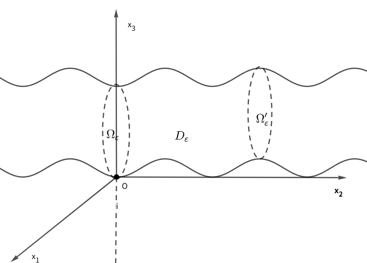
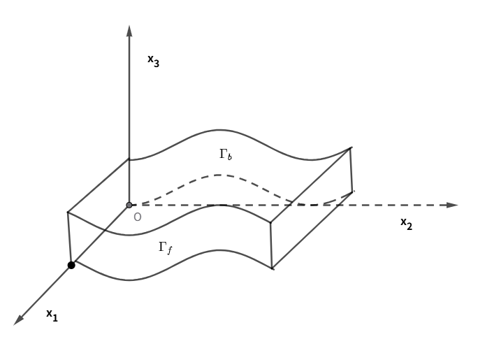
Figure 1. Schematic illustration of the nozzle and slab domains in ℝ3\mathbb{R}^{3}

We now roughly state the main result of the inverse problem outlined in equation (1.4). This result establishes that, under generic conditions, the operators ℱ\mathscr{F} and 𝔣\mathfrak{f}, associated with the constitutive functions 𝐅\mathbf{F} and ff in the system (1.1), can be uniquely and approximately recovered from a single passive measurement ℳℱ,𝔣\mathcal{M}_{\mathscr{F},\mathfrak{f}} on the lateral boundary Γ^×[0,T]\hat{\Gamma}\times[0,T] defined in (1.7).

Theorem 1.2.

Let Ω\Omega be a product-type domain defined in (1.5). Assume that 𝐅j\mathbf{F}^{j} and fjf^{j} belong to the admissible class 𝒜\mathcal{A}, with the corresponding solution uju^{j} in the system (1.1) and the associated operators ℱj\mathscr{F}^{j} and 𝔣j\mathfrak{f}^{j} for j=1,2j=1,2. Let Σ⊂Γ~\Sigma\subset\widetilde{\Gamma}, and let 𝒮\mathcal{S} be an appropriately chosen function space defined on Σ\Sigma. If

ℳℱ1,𝔣1​(u1|Σ)=ℳℱ2,𝔣2​(u2|Σ)for ​uj|Σ∈𝒮,j=1,2,\mathcal{M}_{\mathscr{F}^{1},\mathfrak{f}^{1}}(u^{1}|_{\Sigma})=\mathcal{M}_{\mathscr{F}^{2},\mathfrak{f}^{2}}(u^{2}|_{\Sigma})\quad\text{for }u^{j}|_{\Sigma}\in\mathcal{S},\,j=1,2,

then for any (𝐱,t)∈Q(\mathbf{x},t)\in Q, we obtain

  • (i)

    |ℱ1~​(uj)​(𝐱,t)−ℱ2~​(uj)​(𝐱,t)|≤C​ετ|\tilde{\mathscr{F}^{1}}(u^{j})(\mathbf{x},t)-\tilde{\mathscr{F}^{2}}(u^{j})(\mathbf{x},t)|\leq C\varepsilon^{\tau}, where ℱ1~​(uj)​(𝐱,t)\tilde{\mathscr{F}^{1}}(u^{j})(\mathbf{x},t) and ℱ2~​(uj)​(𝐱,t)\tilde{\mathscr{F}^{2}}(u^{j})(\mathbf{x},t) are related to ℱ1​(uj)​(𝐱,t)\mathscr{F}^{1}(u^{j})(\mathbf{x},t) and ℱ2​(uj)​(𝐱,t)\mathscr{F}^{2}(u^{j})(\mathbf{x},t) for j=1,2j=1,2, respectively.

  • (ii)

    Furthermore, if ℱ1​(u1)​(𝐱,t)=ℱ2​(u2)​(𝐱,t)\mathscr{F}^{1}(u^{1})(\mathbf{x},t)=\mathscr{F}^{2}(u^{2})(\mathbf{x},t), then

    |𝔣1​(uj)​(𝐱,t)−𝔣2​(uj)​(𝐱,t)|≤C′​ετ1.|\mathfrak{f}^{1}(u^{j})(\mathbf{x},t)-\mathfrak{f}^{2}(u^{j})(\mathbf{x},t)|\leq C^{\prime}\varepsilon^{\tau_{1}}.

where τ,τ1∈(0,1)\tau,\tau_{1}\in(0,1), and CC and C′C^{\prime} are positive constants independent of ε\varepsilon.

The precise formulations and detailed analysis of Theorem 1.2 are developed in Section 2. The logical essence of the theorem 1.2 is that when the boundary measurements coincide for two different configurations, the corresponding realizations of the operators acting on two solutions are quantitatively close. Specifically, the difference between ℱ1​(uj)\mathscr{F}^{1}(u^{j}) and ℱ2​(uj)\mathscr{F}^{2}(u^{j}) is bounded by O⁡(ετ)O(\varepsilon^{\tau}), where ε\varepsilon is the geometric parameter characterizing the domain’s small scale and τ\tau is a regularity-dependent exponent. Moreover, under the additional condition that the flux operators produce identical effects on their respective solutions, the corresponding source term realizations 𝔣1​(uj)\mathfrak{f}^{1}(u^{j}) and 𝔣2​(uj)\mathfrak{f}^{2}(u^{j}) are guaranteed to be O⁡(ετ1)O(\varepsilon^{\tau_{1}})-close, where τ1\tau_{1} is an additional regularity parameter.

Remark 1.3.

For the inverse problem in (1.4), we analyze a specialized geometric configuration in which the domain consists of a union of product manifolds 𝒩εℓ=Ωs×Ωr\mathscr{N}_{\varepsilon}^{\ell}=\Omega_{s}\times\Omega_{r}. Such as in ℝ3\mathbb{R}^{3}, Ωs=Ωε\Omega_{s}=\Omega_{\varepsilon} is a two-dimensional manifold which has the hidden dimension, and Ωr=γ⁡(I)\Omega_{r}=\gamma(I) is a one-dimensional manifold, which has the regular dimension. Our main result establishes the unique identifiability of physical processes confined to the hidden dimension Ωs\Omega_{s} from a single passive observation on the boundary ∂Ωs×Ωr\partial\Omega_{s}\times\Omega_{r}, which represents the projection onto the regular dimension Ωr\Omega_{r}. We quantify the the difference between the operators ℱ1\mathscr{F}^{1}, ℱ2\mathscr{F}^{2} (associated with the constitutive function 𝐅\mathbf{F}) and 𝔣1\mathfrak{f}^{1}, 𝔣2\mathfrak{f}^{2} (associated with ff) for the system  (1.1). Under suitable a priori assumptions on 𝐅\mathbf{F} and ff, this bound is controlled by the geometric parameter ε\varepsilon of Ωs\Omega_{s}. This demonstrates that macroscopic variations in the operators are directly influenced by the micro-geometry of the hidden dimension.

1.3. Technical developments and discussion

Nonlinear balance laws provide a versatile framework for modeling diverse physical systems across quantum measurements, gravitational wave detection, fluid dynamics, biological processes, and quantum mechanics, as exemplified by the representative models in Table 1. This paper introduces a unified mathematical framework, described by (1.1), that encapsulates these diverse phenomena. Our primary objective is to develop a robust methodology for identifying nonlinear operators from boundary measurements in multiscale product spaces, offering a cohesive approach to inverse problems spanning multiple physical domains.

Table 1. Summary of PDE Models and Symbols
Model Equation Symbol Meanings
Navier-Stokes ∂t𝐮+(𝐮⋅∇)𝐮=μΔ𝐮−∇p+𝐅\partial_{t}\mathbf{u}+(\mathbf{u}\cdot\nabla)\mathbf{u}=\mu\Delta\mathbf{u}-\nabla p+\mathbf{F} 𝐮\mathbf{u}: velocity, pp: pressure, μ\mu: viscosity
Non-Newtonian ∂t𝐮+∇⋅(μ(|∇𝐮|)∇𝐮)=𝐆\partial_{t}\mathbf{u}+\nabla\cdot(\mu(|\nabla\mathbf{u}|)\nabla\mathbf{u})=\mathbf{G} μ\mu: variable viscosity, 𝐆\mathbf{G}: body force
FitzHugh-Nagumo ∂tu=Δ​u+u⁡(1−u)​(u−a)−v∂tv=ϵ​Δ​v+γ⁡(u−b​v)\begin{aligned} \partial_{t}u&=\Delta u+u(1-u)(u-a)-v\\ \partial_{t}v&=\epsilon\Delta v+\gamma(u-bv)\end{aligned} u,vu,v: potentials; a,b,ϵ,γa,b,\epsilon,\gamma: constants
Chemotaxis ∂tc=∇⋅(D∇c−χ∇ϕ)+R(c)\partial_{t}c=\nabla\cdot(D\nabla c-\chi\nabla\phi)+R(c) cc: density; ϕ\phi: attractant; χ\chi: sensitivity
Magnetic Schrödinger (i∂t+∇⋅𝐀)2ψ+Vψ=0(i\partial_{t}+\nabla\cdot\mathbf{A})^{2}\psi+V\psi=0 ψ\psi: wave function; 𝐀\mathbf{A}: magnetic potential
Ginzburg-Landau ∂tψ=α​Δ​ψ+β​|ψ|2​ψ+γ​𝐀⋅∇ψ\partial_{t}\psi=\alpha\Delta\psi+\beta|\psi|^{2}\psi+\gamma\mathbf{A}\cdot\nabla\psi ψ\psi: order parameter; α,β,γ\alpha,\beta,\gamma: constants

The study of forward problems for general systems of balance laws remains in its nascent stages, with the existing literature primarily focused on specific forms-notably hyperbolic conservation laws, where the flux 𝐅\mathbf{F} and source ff are restricted to particular types. Historical overviews can be found in [8, 12, 22, 25, 31, 32]. Well-posedness proofs for these systems can be broadly classified into two approaches. The first approach addresses the development of singularities, such as shock waves, which emerge in finite time even from smooth, small initial data. This is exemplified in [15] for conservation laws and in [34, 35] for balance laws. The second approach establishes the existence of classical solutions over short time intervals, as demonstrated in [8] for conservation laws and [27] for the Schrödinger equation. Despite these advances, significant open challenges persist, as noted in [31, 32]. Historically, the theory of balance laws has relied heavily on ad hoc methods. These approaches have also been extended to coupled systems, notably in the context of time-dependent mean-field games [5, 6, 1].

Due to the reasons discussed above, inverse problems for the general form of nonlinear balance laws have received considerably less attention. The primary reason for this disparity is straightforward: the mathematical tools and theoretical understanding required to tackle inverse problems robustly are predicated on a well-established theory for the forward problem, which, as discussed, is still taking shape. Most existing results are confined to simpler models and one-dimensional scalar cases, such as the BFGS-based “discretize-then-optimize” strategy [4], Lipschitz stability analysis via Carleman estimates [13], reconstruction methods using front-tracking and Riemann solvers [17], and flux identification from shock asymptotics [20]. Extending these methodologies to higher spatial dimensions, however, introduces substantial theoretical and computational challenges. Key difficulties include the intricate geometry of characteristic networks, the formation of non-planar shocks, complex multi-dimensional wave interactions, and the curse of dimensionality affecting both numerical simulation and parameter space exploration. Moreover, foundational one-dimensional analytical tools, such as the method of characteristics, Riemann solvers, and shock-tracking algorithms do not generalize directly to higher dimensions, further complicating the mathematical analysis.

In this paper, we investigate the inverse problem for the general form of nonlinear balance laws, as presented in (1.1), incorporating source terms in multiple dimensions. As previously highlighted, this problem remains a significant challenge with limited progress in the literature. Our primary focus is the reconstruction of the flux term 𝐅\mathbf{F} and the source term ff in (1.1) using minimal observational data, specifically a single passive boundary measurement. Existing studies, such as [16, 2, 3, 7, 11, 18, 24, 23], predominantly focus on inverse problems for specific forms of the nonlinear balance laws and on recovering explicit analytical forms of 𝐅\mathbf{F} and ff, often relying on strong a priori assumptions, such as specific polynomial structures. However, in practical applications, the input-output behavior of these terms is typically of greater interest than their exact functional forms. This insight drives our novel approach: we reformulate the inverse problem within an operator-theoretic framework, aiming to identify the nonlinear operators ℱ\mathscr{F} and 𝔣\mathfrak{f}, which map the state function uu to the flux and source responses ℱ⁡(u)\mathscr{F}(u) and 𝔣⁡(u)\mathfrak{f}(u), respectively, without requiring explicit analytical representations. This method eliminates the need for restrictive a priori assumptions on functional forms and better aligns with practical scenarios where the system’s behavioral response is the primary concern.

In what follows, we restrict the domain Ω\Omega to the class of product-type domains defined in (1.5)–(1.6). As noted in Remark 1.1, the topological structure of such domains has recently attracted limited but growing attention. Within this geometric setting, several inverse problems have been studied [30, 21, 10, 9]. It is worth emphasizing that our geometric framework for slab-like domains is quite general and does not require the domain to be infinite. Moreover, our framework establishes explicit quantitative relationships between the geometric parameter ε\varepsilon and reconstruction accuracy, elucidating how microscale structures govern the recoverability of nonlinear dynamics from macroscale boundary data. As discussed in Remark 1.3, our work draws a conceptual parallel with the AdS/CFT correspondence in string theory [26, 33, 29], wherein bulk physics is holographically encoded in boundary data.

To establish these results, we first introduce the operators ℱj\mathscr{F}^{j} and 𝔣j\mathfrak{f}^{j}, which correspond to the flux function 𝐅\mathbf{F} and the source term ff, respectively, thereby reformulating the inverse problem within an operator-theoretic framework. Next, we develop complex geometrical optics (CGO) solutions for the underlying balance laws and utilize microlocal analysis to characterize the behavior of ℱj\mathscr{F}^{j} and 𝔣j\mathfrak{f}^{j} in product-type domains. By leveraging the intrinsic geometric properties of these solutions, we achieve an approximate unique determination of both operators from a single local passive measurement.

The remainder of this paper is structured as follows. Section 2 introduces the geometric framework and states the main uniqueness theorems. Section 3 details the two-dimensional proof, including specialized geometric optics solutions and key energy estimates. Section 4 extends the analysis to three-dimensional configurations. Finally, Section 5 demonstrates the applicability of our framework to physical systems, with a focus on reaction-diffusion-convection models.

2. Statement of main results and preliminaries

2.1. Mathematical setup

We mainly restrict our study to the nonlinear system

(2.1) {∂tH⁡(u)+∇𝐱⋅𝐅⁡(𝐱,t,u)=f⁡(𝐱,t,u,∇u)+μ​Δ​uinQ,u⁡(𝐱,t)=𝝍⁡(𝐱,t)onΓ~,\begin{cases}\partial_{t}H(u)+\nabla_{\mathbf{x}}\cdot\mathbf{F}(\mathbf{x},t,u)=f(\mathbf{x},t,u,\nabla u)+\mu\Delta u&\ \text{in}\ \ Q,\\ u(\mathbf{x},t)=\boldsymbol{\psi}(\mathbf{x},t)&\ \text{on}\ \ \widetilde{\Gamma},\end{cases}

where μ∈ℝ+\mu\in\mathbb{R}_{+} is a positive constant, typically representing the viscosity coefficient in fluid mechanics. The terms HH, 𝐅\mathbf{F}, and ff, as defined in (1.1), satisfy essential a priori assumptions critical for tackling the challenges of limited passive boundary measurements, as elaborated in Section 1.1.

Definition 2.1 (Admissible class 𝒜\mathcal{A}).

We say a triplet (H,𝐅,f)∈𝒜(H,\mathbf{F},f)\in\mathcal{A} if they satisfy the following properties:

  • (i)(i)

    The function H:ℂ→ℂH:\mathbb{C}\to\mathbb{C} is Hölder continuous with exponent α1\alpha_{1}, where 0<α1<10<\alpha_{1}<1, i.e., H∈C0,α1​(ℂ)H\in C^{0,\alpha_{1}}(\mathbb{C}).

  • (i​i)(ii)

    The function f:Q×ℂ×ℂ→ℂf:Q\times\mathbb{C}\times\mathbb{C}\to\mathbb{C} is Hölder continuous with exponent α2\alpha_{2}, where 0<α2<10<\alpha_{2}<1, i.e., f∈C0,α2​(Q×ℂ×ℂ)f\in C^{0,\alpha_{2}}(Q\times\mathbb{C}\times\mathbb{C}). Its norm is defined as:

    ‖f‖C0,α2=max\displaystyle\qquad\|f\|_{C^{0,\alpha_{2}}}=\max {sup∥f(⋅,t0,z0,p0)∥C0,α2​(Ω),sup∥f(𝐱0,⋅,z0,p0)∥C0,α2/2​(ℂ),\displaystyle\left\{\sup\|f(\cdot,t_{0},z_{0},p_{0})\|_{C^{0,\alpha_{2}}(\Omega)},\right.\sup\|f(\mathbf{x}_{0},\cdot,z_{0},p_{0})\|_{C^{0,\alpha_{2}/2}(\mathbb{C})},
    sup∥f(𝐱0,t0,⋅,p0)∥C0,α2​(ℂ),sup∥f(𝐱0,t0,z0,⋅)∥C0,α2​(ℂ)},\displaystyle\left.\hskip 5.69046pt\sup\|f(\mathbf{x}_{0},t_{0},\cdot,p_{0})\|_{C^{0,\alpha_{2}}(\mathbb{C})},\sup\|f(\mathbf{x}_{0},t_{0},z_{0},\cdot)\|_{C^{0,\alpha_{2}}(\mathbb{C})}\right\},

    where `​`​s​u​p​"``sup" denotes the supremum taken over all possible values of the corresponding triplet across their entire respective domains. For a fixed (t0,z0,p0)(t_{0},z_{0},p_{0}), the spatial Hölder norm is defined as

    ‖f⁡(⋅,t0,z0,p0)‖C0,α2​(Ω):=‖f‖L∞​(Ω)+sup𝐱≠𝐲|f⁡(𝐱,t0,z0,p0)−f⁡(𝐲,t0,z0,p0)||𝐱−𝐲|α2\qquad\|f(\cdot,t_{0},z_{0},p_{0})\|_{C^{0,\alpha_{2}}(\Omega)}:=\|f\|_{L^{\infty}(\Omega)}+\sup_{\mathbf{x}\neq\mathbf{y}}\frac{|f(\mathbf{x},t_{0},z_{0},p_{0})-f(\mathbf{y},t_{0},z_{0},p_{0})|}{|\mathbf{x}-\mathbf{y}|^{\alpha_{2}}}

    and the other norms are defined analogously for their respective domains.

  • (i​i​i)(iii)

    Each component fkf_{k} of the vector-valued function 𝐅=(fk)k=1n:Q×ℂ→ℂ\mathbf{F}=(f_{k})_{k=1}^{n}:Q\times\mathbb{C}\to\mathbb{C} is Hölder continuous with exponent α3\alpha_{3}, where 0<α3<10<\alpha_{3}<1, i.e., fk∈C0,α3​(Q×ℂ)f_{k}\in C^{0,\alpha_{3}}(Q\times\mathbb{C}) for k=1,…,nk=1,\dots,n.

  • (i​v)(iv)

    For the triplet (H,𝐅,f)(H,\mathbf{F},f) satisfying conditions (i)-(iii), there exists a solution to the boundary value problem (2.1) for some boundary data ψ∈H1/2​(Γ~)\psi\in H^{1/2}(\widetilde{\Gamma}).

Remark 2.1.

As detailed in Subsection 1.3, establishing the existence of solutions to the forward problem for system (2.1) is highly challenging. However, local existence on short-time intervals is a well-established result; see [8, 25, 27, 35] and references therein. Since the inverse problem considered in this paper relies on boundary observations from an arbitrary subinterval [T1,T2]⊂[0,T][T_{1},T_{2}]\subset[0,T], we may, without loss of generality, restrict our analysis to such a short-time interval. Consequently, the existence requirement in condition (iv) of Definition 2.1 is satisfied under the stated regularity assumptions.

In the mathematical framework outlined above, the functions (H,𝐅,f)(H,\mathbf{F},f) are defined through the admissible class 𝒜\mathcal{A} in Definition 2.1. Building upon this functional foundation, we now introduce the corresponding operator structures. As discussed in Section 1.1, we establish the operators ℱ=(ℱk)k=1n\mathscr{F}=(\mathscr{F}_{k})_{k=1}^{n} and 𝔣\mathfrak{f} associated with the flux 𝐅\mathbf{F} and source term ff, respectively. Within this correspondence, the functions 𝐅\mathbf{F} and ff can be viewed as realizations of the operators ℱ\mathscr{F} and 𝔣\mathfrak{f}. Specifically, according to the operator definition in equation (1.3), the components of the vector-valued function 𝐅\mathbf{F} constitute realizations of the operator ℱ=(ℱk)k=1n\mathscr{F}=(\mathscr{F}_{k})_{k=1}^{n}, while the scalar nonlinearity ff represents a realization of the operator 𝔣\mathfrak{f}. Within this operator framework, we can establish the approximate unique identifiability of the inverse problem (1.4) within an a priori admissible class of these functions using a single passive measurement on Σ\Sigma.

Our analysis focuses on recovering the realizations of the operators ℱ\mathscr{F} and 𝔣\mathfrak{f} from a single passive boundary observation. This result shows that we can obtain information in small-scale space Ωε\Omega_{\varepsilon} by observing information in regular-scale space Ωr\Omega_{r}. The following theorem provides a precise formulation of Theorem 1.2.

Theorem 2.2.

Let Ω\Omega be a product-type domain as in (1.5), and let ℳℱj,𝔣j,(j=1,2)\mathcal{M}_{\mathscr{F}^{j},\mathfrak{f}^{j}},\,(j=1,2) be the passive boundary measurement on Γ~\widetilde{\Gamma} corresponding to the triplet (H,𝐅j,fj)∈𝒜(H,\mathbf{F}^{j},f^{j})\in\mathcal{A} and its solution uju^{j} in (2.1), with ℱj\mathscr{F}^{j} and 𝔣j\mathfrak{f}^{j} being the operators associated to 𝐅j\mathbf{F}^{j} and fjf^{j} as defined in (1.3). Assume there exist ε\varepsilon-independent positive constants C1C_{1}, C1′C_{1}^{\prime}, C2C_{2}, C3C_{3}, and C4C_{4}, and Hölder exponents α1,α2,α3,α4∈(0,1)\alpha_{1},\alpha_{2},\alpha_{3},\alpha_{4}\in(0,1) satisfying the following conditions:

  • (i)(i)

    The source term fjf^{j} satisfies

    (2.2) ‖fj‖C0,α2​(Q¯×ℂ×ℂ)≤C2;\|f^{j}\|_{C^{0,\alpha_{2}}(\overline{Q}\times\mathbb{C}\times\mathbb{C})}\leq C_{2};
  • (i​i)(ii)

    The nonlinear terms fkjf_{k}^{j} satisfy for k=1,…,nk=1,\ldots,n:

    (2.3) ‖fkj‖C0,α3​(Q¯×ℂ)≤C3;\|f_{k}^{j}\|_{C^{0,\alpha_{3}}(\overline{Q}\times\mathbb{C})}\leq C_{3};
  • (i​i​i)(iii)

    The solution uju^{j} satisfies

    (2.4) uj∈H1loc(Q)∩C1,α4(Q¯),with∥uj∥C1,α4≤C4.\begin{split}\qquad u^{j}\in H^{1}_{\mathrm{loc}}(Q)\cap C^{1,\alpha_{4}}(\overline{Q}),\,\,\mbox{with}\,\,\|u^{j}\|_{C^{1,\alpha_{4}}}\leq C_{4}.\end{split}

If for any subset Σ⊂Γ~\Sigma\subset\widetilde{\Gamma} and sufficiently small ε\varepsilon, one has

ℳℱ1,𝔣1​(u1|Σ)=ℳℱ2,𝔣2​(u2|Σ),\mathcal{M}_{\mathscr{F}^{1},\mathfrak{f}^{1}}(u^{1}|_{\Sigma})=\mathcal{M}_{\mathscr{F}^{2},\mathfrak{f}^{2}}(u^{2}|_{\Sigma}),

which yields the flux balance condition

(2.5) ∫Σν⋅(𝐅1−𝐅2)​𝑑σ=∫Σμ⁡(h𝐅1−h𝐅2)​𝑑σ,\int_{\Sigma}\nu\cdot(\mathbf{F}^{1}-\mathbf{F}^{2})\,\mathrm{d}\sigma=\int_{\Sigma}\mu(h_{\mathbf{F}^{1}}-h_{\mathbf{F}^{2}})\,\mathrm{d}\sigma,

where ν\nu is the unit outward normal and h𝐅j∈L2​(Q)∩C0,α4​(Q¯)h_{\mathbf{F}^{j}}\in L^{2}(Q)\cap C^{0,\alpha_{4}}(\overline{Q}), then we have

  • (a)(a)

    If ℱ1​(u1)​(𝐱,t)−ℱ2​(u2)​(𝐱,t)≠𝟎\mathscr{F}^{1}(u^{1})(\mathbf{x},t)-\mathscr{F}^{2}(u^{2})(\mathbf{x},t)\neq\mathbf{0} in QQ, suppose the curve γ\gamma defined in Definition 1.1 satisfies the following condition: for some l>0l>0, there exist parameters a1,a2∈Ia_{1},a_{2}\in I such that as long as |a1−a2|≤εl|a_{1}-a_{2}|\leq\varepsilon^{l}, then there must exist b1,b2∈(a1,a2)b_{1},b_{2}\in(a_{1},a_{2}) such that γ′​(b1)\gamma^{\prime}(b_{1}) is parallel to γ′​(b2)\gamma^{\prime}(b_{2}). Furthermore, assume the nonlinear state transfer function HH satisfies

    (2.6) ‖H‖C0,α1​(ℂ)≤C1.\|H\|_{C^{0,\alpha_{1}}(\mathbb{C})}\leq C_{1}.

    Then, for any (𝐱,t)∈Q(\mathbf{x},t)\in Q, there exists a positive constant ε0\varepsilon_{0} such that when ε<ε0\varepsilon<\varepsilon_{0}, the following estimate holds

    (2.7) |ℱ1~(uj)(𝐱,t)−ℱ2~(uj)(𝐱,t)|≤C(ε0,μ,∥h∥L∞,C1,C2,C3,C4)ετ,j=1,2,\left|\tilde{\mathscr{F}^{1}}(u^{j})(\mathbf{x},t)-\tilde{\mathscr{F}^{2}}(u^{j})(\mathbf{x},t)\right|\leq C(\varepsilon_{0},\mu,\|h\|_{L^{\infty}},C_{1},C_{2},C_{3},C_{4})\varepsilon^{\tau},\,\,\,j=1,2,

    where h:=h𝐅1−h𝐅2h:=h_{\mathbf{F}^{1}}-h_{\mathbf{F}^{2}}, C⁡(ε0,μ,‖h‖L∞,C1,C2,C3,C4)C(\varepsilon_{0},\mu,\|h\|_{L^{\infty}},C_{1},C_{2},C_{3},C_{4}) is a generic positive constant depending only on the indicated parameters, and τ\tau is given as follows

    (2.8) τ={α2​α3​l if ​  0<l≤11+α2​α3,12​[1−l⁡(1−α2​α3)] if ​11+α2​α3<l<1,12​(1−l+α2​α3) if ​  1≤l<1+α2​α3.\tau=\begin{cases}\alpha_{2}\alpha_{3}l&\text{ if }\,\,0<l\leq\frac{1}{1+\alpha_{2}\alpha_{3}},\\ \frac{1}{2}\left[1-l\left(1-\alpha_{2}\alpha_{3}\right)\right]&\text{ if }\,\,\frac{1}{1+\alpha_{2}\alpha_{3}}<l<1,\\ \frac{1}{2}\left(1-l+\alpha_{2}\alpha_{3}\right)&\text{ if }\,\,1\leq l<1+\alpha_{2}\alpha_{3}.\end{cases}
  • (b)(b)

    If ℱ1​(u1)​(𝐱,t)−ℱ2​(u2)​(𝐱,t)=𝟎\mathscr{F}^{1}(u^{1})(\mathbf{x},t)-\mathscr{F}^{2}(u^{2})(\mathbf{x},t)=\mathbf{0} and h𝐅1−h𝐅2=0h_{\mathbf{F}^{1}}-h_{\mathbf{F}^{2}}=0 in QQ, assume that for any point 𝐱∈Ω\mathbf{x}\in\Omega, there exists at least one point 𝐱0∈Γ^\mathbf{x}_{0}\in\hat{\Gamma} such that the vector 𝐱−𝐱0\mathbf{x}-\mathbf{x}_{0} is parallel to ν𝐱0\nu_{\mathbf{x}_{0}}, where ν𝐱0\nu_{\mathbf{x}_{0}} is the unit outward normal at 𝐱0\mathbf{x}_{0}. Additionally, the nonlinear state transfer function H∈C1,α1H\in C^{1,\alpha_{1}} satisfies

    (2.9) ‖H‖C1,α1​(ℂ)≤C1′.\|H\|_{C^{1,\alpha_{1}}(\mathbb{C})}\leq C_{1}^{\prime}.

    Then, for any (𝐱,t)∈Q(\mathbf{x},t)\in Q, the following estimate holds

    (2.10) |𝔣1(uj)(𝐱,t)−𝔣2(uj)(𝐱,t)|≤C′(ε0,μ,C1′,C2,C4)ετ1,j=1,2,\hskip 42.67912pt|\mathfrak{f}^{1}(u^{j})(\mathbf{x},t)-\mathfrak{f}^{2}(u^{j})(\mathbf{x},t)|\leq C^{\prime}(\varepsilon_{0},\mu,C_{1}^{\prime},C_{2},C_{4})\varepsilon^{\tau_{1}},\quad j=1,2,

    where C′​(ε0,μ,C1,C2,C3,C4′)C^{\prime}(\varepsilon_{0},\mu,C_{1},C_{2},C_{3},C^{\prime}_{4}) is a generic positive constant depending only on the indicated parameters and τ1=α1​α321+α1​α3\tau_{1}=\frac{\alpha_{1}\alpha_{3}^{2}}{1+\alpha_{1}\alpha_{3}}.

Remark 2.3.

The studied system, described in Subsection 1.1, models the evolution of a scalar state uu within Ω\Omega generated by a physical process, with measurements taken on the boundary Σ\Sigma. The regularity imposed by assumptions (2.2)–(2.4) and (2.6) (or (2.9)) is physically justifiable, as it requires only pointwise bounds—a condition met by many physical processes. This is consistent with the framework of local-time existence outlined in Remark 2.1.

It is important to highlight that the result of the main theorem is non-trivial, even in the case of a linear source term fjf^{j}, namely, fj​(𝐱,t,uj,∇uj)=qj​(𝐱,t)​ujf^{j}(\mathbf{x},t,u^{j},\nabla u^{j})=q^{j}(\mathbf{x},t)u^{j} with qj∈C0,α2​(Q¯)q^{j}\in C^{0,\alpha_{2}}(\overline{Q}). The same boundary observation data (u1,∂νu1+h𝐅1)|Σ=(u2,∂νu2+h𝐅2)|Σ(u^{1},\partial_{\nu}u^{1}+h_{\mathbf{F}^{1}})\big|_{\Sigma}=(u^{2},\partial_{\nu}u^{2}+h_{\mathbf{F}^{2}})\big|_{\Sigma} cannot guarantee that the second- or higher-order derivatives of u1u^{1} and u2u^{2} are pointwise close internally in the product-type domain.

Remark 2.4.

The realizations ℱ1~​(uj)\tilde{\mathscr{F}^{1}}(u^{j}) and ℱ2~​(uj)\tilde{\mathscr{F}^{2}}(u^{j}) in Theorem 2.2(a)(a) are linear combinations of the components of ℱ1​(uj)\mathscr{F}^{1}(u^{j}) and ℱ2​(uj)\mathscr{F}^{2}(u^{j}), respectively, j=1,2j=1,2. Their specific forms depend on the dimension and geometric configuration of Ω\Omega, as follows:

  • (i)

    In ℝ2\mathbb{R}^{2}, the realization take the rotational form:

    ℱ~j(u):=ℱ2j′(u),\tilde{\mathscr{F}}^{j}(u):={\mathscr{F}}^{j\prime}_{2}(u),

    where ℱ2j′(u)\mathscr{F}^{j\prime}_{2}(u) is the second component of ℱj′(u)\mathscr{F}^{j\prime}(u), obtained through coordinate transformation of ℱj​(u)\mathscr{F}^{j}(u). The specific form of ℱ′​(u)\mathscr{F}^{\prime}(u) is given by

    (2.11) ℱj′(u)(𝐱,t):=𝐅j′(𝐱,t,uj)\displaystyle\qquad\mathscr{F}^{j\prime}(u)(\mathbf{x},t):=\mathbf{F}^{j\prime}(\mathbf{x},t,u^{j}) =(f1j′,f2j′)⊤=(f1jcosθ+f2jsinθ,−f1jsinθ+f2jcosθ)⊤.\displaystyle=(f_{1}^{j\prime},f_{2}^{j\prime})^{\top}=(f^{j}_{1}\cos\theta+f^{j}_{2}\sin\theta,-f^{j}_{1}\sin\theta+f^{j}_{2}\cos\theta)^{\top}.
  • (ii)

    In ℝ3\mathbb{R}^{3}, the expressions vary based on the geometric configuration

    ℱ~j(u):=ℱkj′(u),\tilde{\mathscr{F}}^{j}(u):={\mathscr{F}}^{j\prime}_{k}(u),

    where k=1,3k=1,3 for nozzle domain 𝒩εN\mathscr{N}_{\varepsilon}^{N}, and k=3k=3 for slab domain 𝒩εS\mathscr{N}_{\varepsilon}^{S}. The transformed components ℱj′(u):=𝐅j′(𝐱,t,u)=(f1j′,f2j′,f3j′)⊤\mathscr{F}^{j\prime}(u):=\mathbf{F}^{j\prime}(\mathbf{x},t,u)=(f^{j\prime}_{1},f^{j\prime}_{2},f^{j\prime}_{3})^{\top} are given by

    ℱ1j′(u)=f1j′\displaystyle{\mathscr{F}}^{j\prime}_{1}(u)=f_{1}^{j\prime} =f1j​cos⁡β​cos⁡θ+f2j​sin⁡β−f3j​cos⁡β​sin⁡θ,\displaystyle=f^{j}_{1}\cos\beta\cos\theta+f^{j}_{2}\sin\beta-f^{j}_{3}\cos\beta\sin\theta,
    ℱ2j′(u)=f2j′\displaystyle{\mathscr{F}}^{j\prime}_{2}(u)=f_{2}^{j\prime} =−f1j​sin⁡β​cos⁡θ+f2j​cos⁡β+f3j​sin⁡β​sin⁡θ,\displaystyle=-f^{j}_{1}\sin\beta\cos\theta+f^{j}_{2}\cos\beta+f^{j}_{3}\sin\beta\sin\theta,
    (2.12) ℱ3j′(u)=f3j′\displaystyle{\mathscr{F}}^{j\prime}_{3}(u)=f_{3}^{j\prime} =f1j​sin⁡θ+f3j​cos⁡θ.\displaystyle=f^{j}_{1}\sin\theta+f^{j}_{3}\cos\theta.

It is important to note that the rotation angles θ\theta and β\beta in Remark 2.4 are determined by the curve γ\gamma as specified in Theorem 2.2(a)(a). The corresponding coordinate transformations are defined as follows:

  • (i)

    In ℝ2\mathbb{R}^{2}, the coordinate system is translated to a point on γ\gamma (corresponding to parameter b1b_{1}) and rotated clockwise about the origin by an angle θ\theta, aligning the tangent vector γ′​(b1)\gamma^{\prime}(b_{1}) with the x1x_{1}-axis of the new coordinate system. See Figure 2 for an illustration.

  • (ii)

    In ℝ3\mathbb{R}^{3}, the coordinate system is translated to a point on γ\gamma (corresponding to b1b_{1}) and rotated as follows: first, a clockwise rotation by an angle θ\theta about the x2x_{2}-axis, followed by a clockwise rotation by an angle β\beta about the x3x_{3}-axis. This ensures that γ\gamma lies in the x2​x3x_{2}x_{3}-plane and the tangent vector γ′​(b1)\gamma^{\prime}(b_{1}) aligns with the x2x_{2}-axis of the new coordinate system. See Figures 3 and 4 for illustrations.

The proofs of Theorem 2.2 are presented in Sections 3 and 4. To this end, we first introduce the auxiliary tools employed in the proof, focusing on complex geometrical optics solutions and key analytical constructions that play a fundamental role in our approach.

Lemma 2.5 (CGO Solutions).

The exponential function

(2.13) u0​(𝐱,t)=eρμ⋅𝐱+λ​t,ρ=s​𝐝+𝐢​s2+λ​𝐝⟂,u_{0}(\mathbf{x},t)=e^{\frac{\rho}{\sqrt{\mu}}\cdot\mathbf{x}+\lambda t},\quad\rho=s\mathbf{d}+\mathbf{i}\sqrt{s^{2}+\lambda}\mathbf{d}^{\perp},

where 𝐝,𝐝⟂∈𝕊n−1\mathbf{d},\mathbf{d}^{\perp}\in\mathbb{S}^{n-1} satisfy 𝐝⋅𝐝⟂=0\mathbf{d}\cdot\mathbf{d}^{\perp}=0 and μ,s,λ∈ℝ+\mu,s,\lambda\in\mathbb{R}_{+}, has the properties:

(2.14) (∂t+μΔ)u0=0and∂tu0=λu0.(\partial_{t}+\mu\Delta)u_{0}=0\quad\text{and}\quad\partial_{t}u_{0}=\lambda u_{0}.

Another essential tool is the following Green’s formula, which will be used extensively in our energy estimates:

Lemma 2.6 (Space-Time Green’s Formula).

Let Ω⊂ℝn\Omega\subset\mathbb{R}^{n} be a bounded Lipschitz domain and [T1,T2]⊂[0,T][T_{1},T_{2}]\subset[0,T] a time interval. For any functions f,gf,g in the space H1​(Ω×[T1,T2])H^{1}(\Omega\times[T_{1},T_{2}]) with Δ​f,Δ​g∈L2​(Ω×[T1,T2])\Delta f,\,\Delta g\in L^{2}(\Omega\times[T_{1},T_{2}]) and ∂tf,∂tg∈L2​(Ω×[T1,T2])\partial_{t}f,\,\partial_{t}g\in L^{2}(\Omega\times[T_{1},T_{2}]), we have:

∫T1T2∫Ω(g​Δ​f−f​Δ​g)​𝑑𝐱​𝑑t=∫T1T2∫∂Ω(g​∂νf−f​∂νg)​𝑑σ​𝑑t\int_{T_{1}}^{T_{2}}\int_{\Omega}(g\Delta f-f\Delta g)d\mathbf{x}dt=\int_{T_{1}}^{T_{2}}\int_{\partial\Omega}(g\partial_{\nu}f-f\partial_{\nu}g)d\sigma dt

with ν\nu denoting the outward unit normal to ∂Ω\partial\Omega.

3. Proof of Theorem 2.2 in two dimensions

3.1. Geometric Preparation

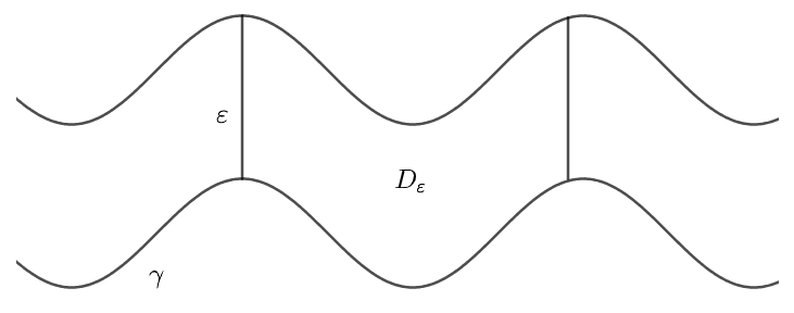
To establish the foundation for proving Theorem 2.2 in the two-dimensional case, we first introduce the key geometric configuration. By the assumption of γ\gamma in Theorem 2.2(a)(a), there are many points on the curve with the same tangent direction, and the radial distance between adjacent points does not exceed εl\varepsilon^{l}. Choose any point, move the original coordinate system to this point and use this point as the new origin, then rotate the coordinate system as described in Remark 2.4. In the new coordinate system, a region of horizontal length εl\varepsilon^{l} is intercepted in 𝒩εℓ⋐Ω\mathscr{N}_{\varepsilon}^{\ell}\Subset\Omega starting from the origin and defined as DεD_{\varepsilon}, see Figure 2 for illustration.

For the remaining part 𝒩εℓ\Dε\mathscr{N}_{\varepsilon}^{\ell}\backslash D_{\varepsilon}, we translate the origin to the next point without rotating the coordinate system and select a new subregion. Since coordinate translation does not alter the form of ∇𝐱⋅𝐅′\nabla_{\mathbf{x}}\cdot\mathbf{F}^{\prime}, we obtain the same result in the new subregion. Repeating this process a finite number of times covers the entire 𝒩εℓ\mathscr{N}_{\varepsilon}^{\ell}. As for the remaining part Ω\𝒩εℓ¯\Omega\backslash\overline{\mathscr{N}_{\varepsilon}^{\ell}}, a similar method can be applied.

In the transformed coordinates, the flux terms become 𝐅′\mathbf{F}^{\prime} and 𝐆′\mathbf{G}^{\prime}, which are defined in (2.11). The boundary ∂Dε\partial D_{\varepsilon} decomposes into four distinct components:

Γ1\displaystyle\Gamma_{1} ={(x1,x2)∣0<x1<εl,x2=γ(x1)},\displaystyle=\{(x_{1},x_{2})\mid 0<x_{1}<\varepsilon^{l},\ x_{2}=\gamma(x_{1})\},
Γ2\displaystyle\Gamma_{2} ={(x1,x2)∣x1=0, 0<x2<ε},\displaystyle=\{(x_{1},x_{2})\mid x_{1}=0,\ 0<x_{2}<\varepsilon\},
Γ3\displaystyle\Gamma_{3} ={(x1,x2)∣0<x1<εl,x2=γ(x1)+ε},\displaystyle=\{(x_{1},x_{2})\mid 0<x_{1}<\varepsilon^{l},\ x_{2}=\gamma(x_{1})+\varepsilon\},
(3.1) Γ4\displaystyle\Gamma_{4} ={(x1,x2)∣x1=εl,γ(εl)<x2<γ(εl)+ε},\displaystyle=\{(x_{1},x_{2})\mid x_{1}=\varepsilon^{l},\ \gamma(\varepsilon^{l})<x_{2}<\gamma(\varepsilon^{l})+\varepsilon\},

where γ\gamma satisfy that

(3.2) |γ|=𝒪⁡(ε),|\gamma|={\mathcal{O}}(\varepsilon),

and for simplicity, we denote

(3.3) l0:=min⁡{l,1},l_{0}:=\min\{l,1\},

where ll is defined in Theorem 2.2, part (a)(a).

Refer to caption
(a) General nozzle configuration in 2D
Refer to caption
(b) Transformed subdomain DεD_{\varepsilon}
Figure 2. configuration for the 2D analysis showing (a) the original nozzle domain and (b) the transformed coordinate system with characteristic subdomain.

To prove the uniqueness of our main results, we derive key estimates for the solution pair of the general coupled PDE system (3.4).

Lemma 3.1.

Let 𝒩εℓ\mathscr{N}_{\varepsilon}^{\ell} be a product-type domain, as specified in (1.6). Suppose that u,v∈Hloc1​(𝒩εℓ×[0,T])∩C1,α4​(𝒩εℓ¯×[0,T])u,v\in H^{1}_{\mathrm{loc}}(\mathscr{N}_{\varepsilon}^{\ell}\times[0,T])\cap C^{1,\alpha_{4}}(\overline{\mathscr{N}_{\varepsilon}^{\ell}}\times[0,T]) with α4∈(0,1)\alpha_{4}\in(0,1) satisfy (2.4) and the coupled system

(3.4) {∂tH⁡(u)−μ​Δ​u=f−∇𝐱⋅𝐅′in ​𝒩εℓ×[0,T],∂tH⁡(v)−μ​Δ​v=g−∇𝐱⋅𝐆′in ​𝒩εℓ×[0,T],u=v,∂νu=∂νv+h⁡(𝐱,t)on ​Γ^×[0,T],\begin{cases}\partial_{t}H(u)-\mu\Delta u=f-\nabla_{\mathbf{x}}\cdot\mathbf{F}^{\prime}&\text{in }\mathscr{N}_{\varepsilon}^{\ell}\times[0,T],\\ \partial_{t}H(v)-\mu\Delta v=g-\nabla_{\mathbf{x}}\cdot\mathbf{G}^{\prime}&\text{in }\mathscr{N}_{\varepsilon}^{\ell}\times[0,T],\\ u=v,\quad\partial_{\nu}u=\partial_{\nu}v+h(\mathbf{x},t)&\text{on }\hat{\Gamma}\times[0,T],\end{cases}

where Γ^\hat{\Gamma} is defined in (1.7). The functions ff and gg satisfy (2.2), while the components of functions 𝐅′\mathbf{F}^{\prime} and 𝐆′\mathbf{G}^{\prime} satisfy (2.3). HH satisfies (2.6) or (2.9), and h∈L2​(𝒩εℓ×[0,T])∩C0,α4​(𝒩εℓ¯×[0,T])h\in L^{2}(\mathscr{N}_{\varepsilon}^{\ell}\times[0,T])\cap C^{0,\alpha_{4}}(\overline{\mathscr{N}_{\varepsilon}^{\ell}}\times[0,T]). Let w=u−vw=u-v. Then ww satisfies

(3.5) {∂t(H⁡(u)−H⁡(v))−μ​Δ​w=(f−g)−∇𝐱⋅(𝐅′−𝐆′)in ​𝒩εℓ×[0,T],w=0,∂νw=h⁡(𝐱,t)on ​Γ^×[0,T].\begin{cases}\partial_{t}(H(u)-H(v))-\mu\Delta w=(f-g)-\nabla_{\mathbf{x}}\cdot(\mathbf{F}^{\prime}-\mathbf{G}^{\prime})&\text{in }\mathscr{N}_{\varepsilon}^{\ell}\times[0,T],\\ w=0,\quad\partial_{\nu}w=h(\mathbf{x},t)&\text{on }\hat{\Gamma}\times[0,T].\end{cases}
Lemma 3.2.

Under the same assumptions on f,gf,g, 𝐅′\mathbf{F}^{\prime}, 𝐆′\mathbf{G}^{\prime} as in Lemma 3.1, let 𝐅′=(f1′,f2′)⊤\mathbf{F}^{\prime}=(f_{1}^{\prime},f_{2}^{\prime})^{\top} and 𝐆′=(g1′,g2′)⊤\mathbf{G}^{\prime}=(g_{1}^{\prime},g_{2}^{\prime})^{\top} be defined by (2.11). For any point (𝐱,t)∈D¯ε×[T1,T2]⊂𝒩εℓ×[0,T](\mathbf{x},t)\in\overline{D}_{\varepsilon}\times[T_{1},T_{2}]\subset\mathscr{N}_{\varepsilon}^{\ell}\times[0,T], with T2−T1=ε2T_{2}-T_{1}=\varepsilon^{2} and ε\varepsilon being the geometric parameter, the following expansions hold

f⁡(𝐱,t,u,∇u)−g⁡(𝐱,t,v,∇v)\displaystyle f(\mathbf{x},t,u,\nabla u)-g(\mathbf{x},t,v,\nabla v) =(f−g)(𝐱,t)=(𝐱0,t0)+δf​f−δg​g\displaystyle=(f-g)_{(\mathbf{x},t)=(\mathbf{x}_{0},t_{0})}+\delta_{f}f-\delta_{g}g
≔(f−g)(𝐱,t)=(𝐱0,t0)+δ0​(f−g),\displaystyle\coloneqq(f-g)_{(\mathbf{x},t)=(\mathbf{x}_{0},t_{0})}+\delta_{0}(f-g),
fk′​(𝐱,t,u)−gk′​(𝐱,t,v)\displaystyle f_{k}^{\prime}(\mathbf{x},t,u)-g_{k}^{\prime}(\mathbf{x},t,v) =(fk′−gk′)(𝐱,t)=(𝐱0,t0)+δfk′​fk′−δgk′​gk′\displaystyle=(f_{k}^{\prime}-g_{k}^{\prime})_{(\mathbf{x},t)=(\mathbf{x}_{0},t_{0})}+\delta_{f_{k}^{\prime}}f_{k}^{\prime}-\delta_{g_{k}^{\prime}}g_{k}^{\prime}
≔(fk′−gk′)(𝐱,t)=(𝐱0,t0)+δk​(fk′−gk′).\displaystyle\coloneqq(f_{k}^{\prime}-g_{k}^{\prime})_{(\mathbf{x},t)=(\mathbf{x}_{0},t_{0})}+\delta_{k}(f_{k}^{\prime}-g_{k}^{\prime}).

Furthermore, the remainder terms satisfy the estimates:

|δ0​(f−g)|\displaystyle|\delta_{0}(f-g)| ≤C⁡(C2,C4)​(|𝐱−𝐱0|+|t−t0|1/2)α2​α4,\displaystyle\leq C(C_{2},C_{4})\big(|\mathbf{x}-\mathbf{x}_{0}|+|t-t_{0}|^{1/2}\big)^{\alpha_{2}\alpha_{4}},
|δk​(fk′−gk′)|\displaystyle|\delta_{k}(f_{k}^{\prime}-g_{k}^{\prime})| ≤C⁡(C3,C4)​(|𝐱−𝐱0|+|t−t0|1/2)α3​α4,\displaystyle\leq C(C_{3},C_{4})\big(|\mathbf{x}-\mathbf{x}_{0}|+|t-t_{0}|^{1/2}\big)^{\alpha_{3}\alpha_{4}},

where (𝐱0,t0)∈D¯ε×[T1,T2](\mathbf{x}_{0},t_{0})\in\overline{D}_{\varepsilon}\times[T_{1},T_{2}], |⋅||\cdot| denotes the Euclidean distance, αi∈(0,1)\alpha_{i}\in(0,1) for i=2,3,4i=2,3,4, and the constants CiC_{i} (i=2,3,4i=2,3,4) are as defined in (2.2), (2.3), and (2.4), respectively.

These expansions will enable us to carefully track the dependence on geometric parameter ε\varepsilon in our estimates. With these preparatory results established, we now derive a key integral identity that connects boundary behavior to interior quantities. This identity, which follows from careful application of Green’s theorem, will be central to our analysis.

Lemma 3.3.

Consider the nonlinear system (3.5) and under the same setup as in Lemma 3.1, using the CGO solution u0u_{0} from (2.13) with direction 𝐝=(d1,d2)\mathbf{d}=(d_{1},d_{2}) where d1,d2<0d_{1},d_{2}<0, and for any time interval [T1,T2]⊂[0,T][T_{1},T_{2}]\subset[0,T] with T2−T1=ε2T_{2}-T_{1}=\varepsilon^{2}, we have the identity:

(3.6) I1+I2=I3+I4−I5−I6,I_{1}+I_{2}=I_{3}+I_{4}-I_{5}-I_{6},

where

I1=\displaystyle I_{1}= μ​∫T1T2∫Γ2∪Γ4(w​∂νu0−u0​∂νw)​𝑑σ​𝑑t,\displaystyle\mu\int_{T_{1}}^{T_{2}}\int_{\Gamma_{2}\cup\Gamma_{4}}(w\partial_{\nu}u_{0}-u_{0}\partial_{\nu}w)\mathrm{d}\sigma\mathrm{d}t, I2=∫T1T2∫Γ2∪Γ4ν⋅(𝐅′−𝐆′)​u0​𝑑σ​𝑑t,\displaystyle I_{2}=\int_{T_{1}}^{T_{2}}\int_{\Gamma_{2}\cup\Gamma_{4}}\nu\cdot(\mathbf{F}^{\prime}-\mathbf{G}^{\prime})u_{0}\mathrm{d}\sigma\mathrm{d}t,
I3=\displaystyle I_{3}= ∫T1T2∫Dε(f−g)​u0​𝑑𝐱​𝑑t,\displaystyle\int_{T_{1}}^{T_{2}}\int_{D_{\varepsilon}}(f-g)u_{0}\mathrm{d}\mathbf{x}\mathrm{d}t, I4=∫T1T2∫Dε(𝐅′−𝐆′)⋅∇u0​𝑑𝐱​𝑑t,\displaystyle I_{4}=\int_{T_{1}}^{T_{2}}\int_{D_{\varepsilon}}(\mathbf{F}^{\prime}-\mathbf{G}^{\prime})\cdot\nabla u_{0}\mathrm{d}\mathbf{x}\mathrm{d}t,
I5=\displaystyle I_{5}= ∫Dε(H⁡(u)−H⁡(v))​u0|T1T2​𝑑𝐱,\displaystyle\int_{D_{\varepsilon}}(H(u)-H(v))u_{0}|_{T_{1}}^{T_{2}}\mathrm{d}\mathbf{x}, I6=∫T1T2∫Dελ⁡(w−(H⁡(u)−H⁡(v)))​u0​𝑑𝐱​𝑑t.\displaystyle I_{6}=\int_{T_{1}}^{T_{2}}\int_{D_{\varepsilon}}\lambda(w-(H(u)-H(v)))u_{0}\mathrm{d}\mathbf{x}\mathrm{d}t.
Proof.

By applying Lemma 2.6, the CGO solution in (2.14), the geometry in (3.1), and the boundary conditions from (3.5), we obtain

∫T1T2∫Dε(∂t(H⁡(u)−H⁡(v))−μ​Δ​w)​u0+(∂tu0+μ​Δ​u0)​w​𝑑𝐱​𝑑t\displaystyle\int_{T_{1}}^{T_{2}}\int_{D_{\varepsilon}}(\partial_{t}(H(u)-H(v))-\mu\Delta w)u_{0}+(\partial_{t}u_{0}+\mu\Delta u_{0})w\mathrm{d}\mathbf{x}\mathrm{d}t
=\displaystyle= ∫T1T2∫∂Dεμ⁡(w​∂νu0−u0​∂νw)​𝑑σ​𝑑t+∫Dε(H⁡(u)−H⁡(v))​u0|T1T2​𝑑𝐱\displaystyle\int_{T_{1}}^{T_{2}}\int_{\partial D_{\varepsilon}}\mu(w\partial_{\nu}u_{0}-u_{0}\partial_{\nu}w)\mathrm{d}\sigma\mathrm{d}t+\int_{D_{\varepsilon}}(H(u)-H(v))u_{0}|_{T_{1}}^{T_{2}}\mathrm{d}\mathbf{x}
+∫T1T2∫Dε(w−(H(u)−H(v)))∂tu0d𝐱dt\displaystyle+\int_{T_{1}}^{T_{2}}\int_{D_{\varepsilon}}(w-(H(u)-H(v)))\partial_{t}u_{0}\mathrm{d}\mathbf{x}\mathrm{d}t
=\displaystyle= μ​∫T1T2[∫Γ2∪Γ4(w​∂νu0−u0​∂νw)​𝑑σ−∫Γ1∪Γ3u0​h​(u,v)​𝑑σ]​𝑑t\displaystyle\mu\int_{T_{1}}^{T_{2}}\big[\int_{\Gamma_{2}\cup\Gamma_{4}}(w\partial_{\nu}u_{0}-u_{0}\partial_{\nu}w)\mathrm{d}\sigma-\int_{\Gamma_{1}\cup\Gamma_{3}}u_{0}h(u,v)\mathrm{d}\sigma\big]\mathrm{d}t
(3.7) +∫Dε(H(u)−H(v))u0|T1T2d𝐱+∫T1T2∫Dελ(w−(H(u)−H(v)))u0d𝐱dt.\displaystyle+\int_{D_{\varepsilon}}(H(u)-H(v))u_{0}|_{T_{1}}^{T_{2}}\mathrm{d}\mathbf{x}+\int_{T_{1}}^{T_{2}}\int_{D_{\varepsilon}}\lambda(w-(H(u)-H(v)))u_{0}\mathrm{d}\mathbf{x}\mathrm{d}t.

On the other hand, using (2.5), (2.14), and (3.5), we can drive that

∫T1T2∫Dε(∂t(H⁡(u)−H⁡(v))−μ​Δ​w)​u0+(∂tu0+μ​Δ​u0)​w​𝑑𝐱​𝑑t\displaystyle\int_{T_{1}}^{T_{2}}\int_{D_{\varepsilon}}(\partial_{t}(H(u)-H(v))-\mu\Delta w)u_{0}+(\partial_{t}u_{0}+\mu\Delta u_{0})w\mathrm{d}\mathbf{x}\mathrm{d}t
=\displaystyle= ∫T1T2∫Dε(∂t(H⁡(u)−H⁡(v))−μ​Δ​w)​u0​𝑑𝐱​𝑑t\displaystyle\int_{T_{1}}^{T_{2}}\int_{D_{\varepsilon}}(\partial_{t}(H(u)-H(v))-\mu\Delta w)u_{0}\mathrm{d}\mathbf{x}\mathrm{d}t
=\displaystyle= ∫T1T2∫Dε(f−g)​u0​𝑑𝐱​𝑑t−∫T1T2∫Dε∇𝐱⋅(𝐅′−𝐆′)​u0​𝑑𝐱​𝑑t\displaystyle\int_{T_{1}}^{T_{2}}\int_{D_{\varepsilon}}(f-g)u_{0}\mathrm{d}\mathbf{x}\mathrm{d}t-\int_{T_{1}}^{T_{2}}\int_{D_{\varepsilon}}\nabla_{\mathbf{x}}\cdot(\mathbf{F}^{\prime}-\mathbf{G}^{\prime})u_{0}\mathrm{d}\mathbf{x}\mathrm{d}t
=\displaystyle= ∫T1T2∫Dε(f−g)​u0​𝑑𝐱​𝑑t−∫T1T2∫∂Dεν⋅(𝐅′−𝐆′)​u0​𝑑σ​𝑑t\displaystyle\int_{T_{1}}^{T_{2}}\int_{D_{\varepsilon}}(f-g)u_{0}\mathrm{d}\mathbf{x}\mathrm{d}t-\int_{T_{1}}^{T_{2}}\int_{\partial D_{\varepsilon}}\nu\cdot(\mathbf{F}^{\prime}-\mathbf{G}^{\prime})u_{0}\mathrm{d}\sigma\mathrm{d}t
+∫T1T2∫Dε(𝐅′−𝐆′)⋅∇u0d𝐱dt\displaystyle+\int_{T_{1}}^{T_{2}}\int_{D_{\varepsilon}}(\mathbf{F}^{\prime}-\mathbf{G}^{\prime})\cdot\nabla u_{0}\mathrm{d}\mathbf{x}\mathrm{d}t
=\displaystyle= ∫T1T2∫Dε(f−g)​u0​𝑑𝐱​𝑑t+∫T1T2∫Dε(𝐅′−𝐆′)⋅∇u0​𝑑𝐱​𝑑t\displaystyle\int_{T_{1}}^{T_{2}}\int_{D_{\varepsilon}}(f-g)u_{0}\mathrm{d}\mathbf{x}\mathrm{d}t+\int_{T_{1}}^{T_{2}}\int_{D_{\varepsilon}}(\mathbf{F}^{\prime}-\mathbf{G}^{\prime})\cdot\nabla u_{0}\mathrm{d}\mathbf{x}\mathrm{d}t
(3.8) −∫T1T2[∫Γ2∪Γ4ν⋅(𝐅′−𝐆′)u0dσ+μ∫Γ1∪Γ3u0h(u,v)dσ]dt.\displaystyle-\int_{T_{1}}^{T_{2}}\big[\int_{\Gamma_{2}\cup\Gamma_{4}}\nu\cdot(\mathbf{F}^{\prime}-\mathbf{G}^{\prime})u_{0}\mathrm{d}\sigma+\mu\int_{\Gamma_{1}\cup\Gamma_{3}}u_{0}h(u,v)\mathrm{d}\sigma\big]\mathrm{d}t.

Equating expressions (3.7) and (3.8) and analyzing the boundary terms yields the desired identity (3.6). ∎

These terms will be carefully estimated in the following process to establish our main results. For the CGO solution u0u_{0} defined in (2.13) in two dimensions, we take 𝐝=(d1,d2)\mathbf{d}=(d_{1},d_{2}) with d1,d2<0d_{1},d_{2}<0 and 𝐝⊥=(d2,−d1)\mathbf{d}^{\bot}=(d_{2},-d_{1}), then we get

u0​(𝐱,t)\displaystyle u_{0}(\mathbf{x},t) =eλ​t​eμ−12​(s​d1+𝐢​s2+λ​d2)​x1+μ−12​(s​d2−𝐢​s2+λ​d1)​x2,\displaystyle=e^{\lambda t}e^{\mu^{-\frac{1}{2}}(sd_{1}+\mathbf{i}\sqrt{s^{2}+\lambda}d_{2})x_{1}+\mu^{-\frac{1}{2}}(sd_{2}-\mathbf{i}\sqrt{s^{2}+\lambda}d_{1})x_{2}},
(3.9) ∇u0​(𝐱,t)\displaystyle\nabla u_{0}(\mathbf{x},t) =μ−12​(s​d1+𝐢​s2+λ​d2,s​d2−𝐢​s2+λ​d1)⊤​u0​(𝐱,t).\displaystyle=\mu^{-\frac{1}{2}}(sd_{1}+\mathbf{i}\sqrt{s^{2}+\lambda}d_{2},sd_{2}-\mathbf{i}\sqrt{s^{2}+\lambda}d_{1})^{\top}u_{0}(\mathbf{x},t).

In the subsequent analysis, we consider s=ε−βs=\varepsilon^{-\beta} for some β>0\beta>0 satisfying the conditions

(3.10) β≤l​ and ​β<1.\beta\leq l\,\text{~and~}\,\beta<1.
Lemma 3.4.

The boundary integral term I1I_{1} defined in (3.6) admits the following asymptotic estimate:

(3.11) |I1|≤C⁡(μ,‖h‖L∞,C4)​(s2​ε3+l+s2​ε2+l+(1+α4)​l0+ε2+α4​l0)+𝒪⁡(s3​ε3+2​l)+𝒪⁡(s​ε3+α4​l0),|I_{1}|\leq C(\mu,\|h\|_{L^{\infty}},C_{4})(s^{2}\varepsilon^{3+l}+s^{2}\varepsilon^{2+l+(1+\alpha_{4})l_{0}}+\varepsilon^{2+\alpha_{4}l_{0}})+\mathcal{O}(s^{3}\varepsilon^{3+2l})+\mathcal{O}(s\varepsilon^{3+\alpha_{4}l_{0}}),

where l0l_{0} is defined in (3.3), and positive constant C⁡(μ,‖h‖L∞,C4)C(\mu,\|h\|_{L^{\infty}},C_{4}) depends only on μ\mu, ‖h‖L∞\|h\|_{L^{\infty}}, and C4C_{4}.

Proof.

Using the boundary condition w=0w=0 on Γ^×[T1,T2]\hat{\Gamma}\times[T_{1},T_{2}], it follows that the tangential derivative of ww along the boundary curve γ\gamma and any time derivative on the boundary vanish. Namely, ∂tw⁡(𝐱,t)=0\partial_{t}w(\mathbf{x},t)=0 for 𝐱∈Γ^\mathbf{x}\in\hat{\Gamma}. In the transformed coordinate system, this implies ∂1w⁡(𝟎,t)=0\partial_{1}w(\mathbf{0},t)=0. Moreover, based on Lemma 3.1, we have w∈C1,α4​(D¯ε×[T1,T2])w\in C^{1,\alpha_{4}}(\overline{D}_{\varepsilon}\times[T_{1},T_{2}]). From the geometric framework in (3.1), we derive the expansion for any point (𝐱,t)∈Γ2×[T1,T2](\mathbf{x},t)\in\Gamma_{2}\times[T_{1},T_{2}] as ε≪1\varepsilon\ll 1:

w⁡(𝐱,t)\displaystyle w(\mathbf{x},t) =w⁡(𝟎,t0)+(0,x2)⋅(∂1w⁡(𝟎,t0),∂2w⁡(𝟎,t0))+∂tw⁡(𝟎,t0)​(t−t0)+ℛw|Γ2\displaystyle=w(\mathbf{0},t_{0})+(0,x_{2})\cdot(\partial_{1}w(\mathbf{0},t_{0}),\partial_{2}w(\mathbf{0},t_{0}))+\partial_{t}w(\mathbf{0},t_{0})(t-t_{0})+\mathcal{R}_{w|\Gamma_{2}}
(3.12) =−h​(𝟎,u,v)(𝐱,t)=(𝟎,t0)​x2+ℛw|Γ2,\displaystyle=-h(\mathbf{0},u,v)_{(\mathbf{x},t)=(\mathbf{0},t_{0})}x_{2}+\mathcal{R}_{w|\Gamma_{2}},
∂νw⁡(𝐱,t)\displaystyle\partial_{\nu}w(\mathbf{x},t) =(−1,0)⋅(∂1w(𝐱,t),∂2w(𝐱,t))=−∂1w(𝐱,t)\displaystyle=(-1,0)\cdot(\partial_{1}w(\mathbf{x},t),\partial_{2}w(\mathbf{x},t))=-\partial_{1}w(\mathbf{x},t)
=−∂1w(𝟎,t0)+ℛ∂w|Γ2=ℛ∂w|Γ2,\displaystyle=-\partial_{1}w(\mathbf{0},t_{0})+\mathcal{R}_{\partial w|\Gamma_{2}}=\mathcal{R}_{\partial w|\Gamma_{2}},
(3.13) ∂νu0\displaystyle\partial_{\nu}u_{0} =−μ−12​(s​d1+𝐢​s2+λ​d2)​eλ​t​eμ−12​(s​d2−𝐢​s2+λ​d1)​x2,\displaystyle=-\mu^{-\frac{1}{2}}(sd_{1}+\mathbf{i}\sqrt{s^{2}+\lambda}d_{2})e^{\lambda t}e^{\mu^{-\frac{1}{2}}(sd_{2}-\mathbf{i}\sqrt{s^{2}+\lambda}d_{1})x_{2}},

where

|ℛw|Γ2|\displaystyle|\mathcal{R}_{w|\Gamma_{2}}| ≤C4​(|𝐱|+|t−t0|12)1+α4≤C4​ε1+α4,\displaystyle\leq C_{4}(|\mathbf{x}|+|t-t_{0}|^{\frac{1}{2}})^{1+\alpha_{4}}\leq C_{4}\varepsilon^{1+\alpha_{4}},
(3.14) |ℛ∂w|Γ2|\displaystyle|\mathcal{R}_{\partial w|\Gamma_{2}}| ≤C4​(|𝐱|+|t−t0|12)α4≤C4​εα4,\displaystyle\leq C_{4}(|\mathbf{x}|+|t-t_{0}|^{\frac{1}{2}})^{\alpha_{4}}\leq C_{4}\varepsilon^{\alpha_{4}},

for some t0∈[T1,T2]t_{0}\in[T_{1},T_{2}] and T2−T1=ε2T_{2}-T_{1}=\varepsilon^{2}.

Similarly, for any point (𝐱,t)∈Γ4×[T1,T2](\mathbf{x},t)\in\Gamma_{4}\times[T_{1},T_{2}] for ε≪1\varepsilon\ll 1, we obtain:

w⁡(𝐱,t)\displaystyle w(\mathbf{x},t) =w⁡(𝟎,t0)+(εl,x2)⋅(∂1w⁡(𝟎,t0),∂2w⁡(𝟎,t0))+∂tw⁡(𝟎,t0)​(t−t0)+ℛw|Γ4\displaystyle=w(\mathbf{0},t_{0})+(\varepsilon^{l},x_{2})\cdot(\partial_{1}w(\mathbf{0},t_{0}),\partial_{2}w(\mathbf{0},t_{0}))+\partial_{t}w(\mathbf{0},t_{0})(t-t_{0})+\mathcal{R}_{w|\Gamma_{4}}
(3.15) =−h​(𝟎,u,v)(𝐱,t)=(𝟎,t0)​x2+ℛw|Γ4,\displaystyle=-h(\mathbf{0},u,v)_{(\mathbf{x},t)=(\mathbf{0},t_{0})}x_{2}+\mathcal{R}_{w|\Gamma_{4}},
∂νw⁡(𝐱,t)\displaystyle\partial_{\nu}w(\mathbf{x},t) =(1,0)⋅(∂1w⁡(𝐱,t),∂2w⁡(𝐱,t))=∂1w⁡(𝐱,t)\displaystyle=(1,0)\cdot(\partial_{1}w(\mathbf{x},t),\partial_{2}w(\mathbf{x},t))=\partial_{1}w(\mathbf{x},t)
=∂1w⁡(𝟎,t0)+ℛ∂w|Γ4=ℛ∂w|Γ4,\displaystyle=\partial_{1}w(\mathbf{0},t_{0})+\mathcal{R}_{\partial w|\Gamma_{4}}=\mathcal{R}_{\partial w|\Gamma_{4}},
(3.16) ∂νu0\displaystyle\partial_{\nu}u_{0} =μ−12​(s​d1+𝐢​s2+λ​d2)​eλ​t​eμ−12​(s​d2−𝐢​s2+λ​d1)​x2​eμ−12​(s​d1+𝐢​s2+λ​d2)​εl,\displaystyle=\mu^{-\frac{1}{2}}(sd_{1}+\mathbf{i}\sqrt{s^{2}+\lambda}d_{2})e^{\lambda t}e^{\mu^{-\frac{1}{2}}(sd_{2}-\mathbf{i}\sqrt{s^{2}+\lambda}d_{1})x_{2}}e^{\mu^{-\frac{1}{2}}(sd_{1}+\mathbf{i}\sqrt{s^{2}+\lambda}d_{2})\varepsilon^{l}},

where

|ℛw|Γ4|\displaystyle|\mathcal{R}_{w|\Gamma_{4}}| ≤C4​(|(εl,x2)|+|t−t0|12)1+α4≤C4​ε(1+α4)​l0,\displaystyle\leq C_{4}\big(|(\varepsilon^{l},x_{2})|+|t-t_{0}|^{\frac{1}{2}}\big)^{1+\alpha_{4}}\leq C_{4}\varepsilon^{(1+\alpha_{4})l_{0}},
(3.17) |ℛ∂w|Γ4|\displaystyle|\mathcal{R}_{\partial w|\Gamma_{4}}| ≤C4​(|(εl,x2)|+|t−t0|12)α4≤C4​εα4​l0,\displaystyle\leq C_{4}\big(|(\varepsilon^{l},x_{2})|+|t-t_{0}|^{\frac{1}{2}}\big)^{\alpha_{4}}\leq C_{4}\varepsilon^{\alpha_{4}l_{0}},

with l0l_{0} defined in (3.3). Therefore, combining (3.12), (3.13), (3.15), and (3.16), we have the following estimate:

|∫T1T2∫Γ2∪Γ4w​∂νu0​𝑑σ​𝑑t|\displaystyle\left|\int_{T_{1}}^{T_{2}}\int_{\Gamma_{2}\cup\Gamma_{4}}w\partial_{\nu}u_{0}\mathrm{d}\sigma\mathrm{d}t\right|
≤|μ−12​(s​d1+𝐢​s2+λ​d2)​(eμ−12​(s​d1+𝐢​s2+λ​d2)​εl−1)​eλ​T1λ​(eλ​ε−1)\displaystyle\leq\bigg|\mu^{-\frac{1}{2}}(sd_{1}+\mathbf{i}\sqrt{s^{2}+\lambda}d_{2})(e^{\mu^{-\frac{1}{2}}(sd_{1}+\mathbf{i}\sqrt{s^{2}+\lambda}d_{2})\varepsilon^{l}}-1)\frac{e^{\lambda T_{1}}}{\lambda}(e^{\lambda\varepsilon}-1)
(3.18) ×∫0ε(−h(𝟎,u,v)(𝐱,t)=(𝟎,t0)x2+C4(ε(1+α4)​l0))eμ−12​(s​d2−𝐢​s2+λ​d1)​x2dx2|.\displaystyle\quad\times\int_{0}^{\varepsilon}\left(-h(\mathbf{0},u,v)_{(\mathbf{x},t)=(\mathbf{0},t_{0})}x_{2}+C_{4}(\varepsilon^{(1+\alpha_{4})l_{0}})\right)e^{\mu^{-\frac{1}{2}}(sd_{2}-\mathbf{i}\sqrt{s^{2}+\lambda}d_{1})x_{2}}\mathrm{d}x_{2}\bigg|.

By incorporating the CGO parameter ss from (3.10), we obtain

|s​d1+i​s2+λ​d2|≤s2+λ,\displaystyle|sd_{1}+i\sqrt{s^{2}+\lambda}d_{2}|\leq\sqrt{s^{2}+\lambda},
eμ−12​s​d2​ε=1+μ−12​s​d2​ε+(μ−12​s​d2​ε)22+𝒪⁡(s3​ε3),\displaystyle e^{\mu^{-\frac{1}{2}}sd_{2}\varepsilon}=1+\mu^{-\frac{1}{2}}sd_{2}\varepsilon+\frac{(\mu^{-\frac{1}{2}}sd_{2}\varepsilon)^{2}}{2}+{\mathcal{O}}(s^{3}\varepsilon^{3}),
(3.19) |1−eμ−12​(s​d1+𝐢​s2+λ​d2)​εl|≤(eμ−12​1+λ−1)​s​εl.\displaystyle|1-e^{\mu^{-\frac{1}{2}}(sd_{1}+\mathbf{i}\sqrt{s^{2}+\lambda}d_{2})\varepsilon^{l}}|\leq(e^{\mu^{-\frac{1}{2}}\sqrt{1+\lambda}}-1)s\varepsilon^{l}.

Next we estimate part of integral formula (3.18) further,

|∫0εx2​eμ−12​(s​d2−𝐢​s2+λ​d1)​x2​d​x2|≤∫0εx2​eμ−12​s​d2​x2​d​x2\displaystyle\left|\int_{0}^{\varepsilon}x_{2}e^{\mu^{-\frac{1}{2}}(sd_{2}-\mathbf{i}\sqrt{s^{2}+\lambda}d_{1})x_{2}}\mathrm{d}x_{2}\right|\leq\int_{0}^{\varepsilon}x_{2}e^{\mu^{-\frac{1}{2}}sd_{2}x_{2}}\mathrm{d}x_{2}
(3.20) ≤|eμ−12​s​d2​ε​(μ−12​s​d2​ε−1)+1(μ−12​s​d2)2|=ε22+𝒪⁡(s​ε3).\displaystyle\leq\bigg|\frac{e^{\mu^{-\frac{1}{2}}sd_{2}\varepsilon}(\mu^{-\frac{1}{2}}sd_{2}\varepsilon-1)+1}{(\mu^{-\frac{1}{2}}sd_{2})^{2}}\bigg|=\frac{\varepsilon^{2}}{2}+\mathcal{O}(s\varepsilon^{3}).

Similarly, we have

(3.21) |∫0εe(s​d2−𝐢​s2+λ​d1)​x2​μ−12​d​x2|≤ε+𝒪⁡(s​ε2).\left|\int_{0}^{\varepsilon}e^{(sd_{2}-\mathbf{i}\sqrt{s^{2}+\lambda}d_{1})x_{2}\mu^{-\frac{1}{2}}}\mathrm{d}x_{2}\right|\leq\varepsilon+\mathcal{O}(s\varepsilon^{2}).

Combining (3.18), (3.19), (3.20), and (3.21), we obtain

|∫T1T2∫Γ2∪Γ4w​∂νu0​d​x2​𝑑t|≤\displaystyle\left|\int_{T_{1}}^{T_{2}}\int_{\Gamma_{2}\cup\Gamma_{4}}w\partial_{\nu}u_{0}\mathrm{d}x_{2}\mathrm{d}t\right|\leq μ−12​|h​(𝟎,u,v)(𝐱,t)=(𝟎,t0)|​eλ​T12​s2​εl+3\displaystyle\frac{\mu^{-\frac{1}{2}}|h(\mathbf{0},u,v)_{(\mathbf{x},t)=(\mathbf{0},t_{0})}|e^{\lambda T_{1}}}{2}s^{2}\varepsilon^{l+3}
(3.22) +C4​μ−12​eλ​T1​s2​ε2+l+(1+α4)​l0+𝒪⁡(s3​ε3+2​l).\displaystyle+C_{4}\mu^{-\frac{1}{2}}e^{\lambda T_{1}}s^{2}\varepsilon^{2+l+(1+\alpha_{4})l_{0}}+\mathcal{O}(s^{3}\varepsilon^{3+2l}).

Likewise, we have the following estimate:

|∫T1T2∫Γ2∪Γ4u0​∂νw​d​x2​𝑑t|≤\displaystyle\left|\int_{T_{1}}^{T_{2}}\int_{\Gamma_{2}\cup\Gamma_{4}}u_{0}\partial_{\nu}w\mathrm{d}x_{2}\mathrm{d}t\right|\leq C4​εα4​l0​|∫T1T2∫0εeλ​t​eμ−12​s​d2​x2​(1+eμ−12​s​d1​εl)​d​x2​𝑑t|\displaystyle C_{4}\varepsilon^{\alpha_{4}l_{0}}\bigg|\int_{T_{1}}^{T_{2}}\int_{0}^{\varepsilon}e^{\lambda t}e^{\mu^{-\frac{1}{2}}sd_{2}x_{2}}(1+e^{\mu^{-\frac{1}{2}}sd_{1}\varepsilon^{l}})\mathrm{d}x_{2}\mathrm{d}t\bigg|
(3.23) ≤C4​eλ​T1​ε2+α4​l0+𝒪⁡(s​ε3+α4​l0).\displaystyle\leq C_{4}e^{\lambda T_{1}}\varepsilon^{2+\alpha_{4}l_{0}}+\mathcal{O}(s\varepsilon^{3+\alpha_{4}l_{0}}).

Combining (3.22) and (3.23), it yields the desired bound (3.11). ∎

Lemma 3.5.

The term I2I_{2}, defined in (3.6), can be decomposed as

(3.24) I2=I21+I22,I_{2}=I_{21}+I_{22},

with

I21=\displaystyle I_{21}= (f1′−g1′)(𝐱,t)=(𝟎,t0)λ⁡(s​d2−𝐢​s2+λ​d1)​eλ​T1​(eλ​ε−1)​(e(s​d1+𝐢​s2+λ​d2)​εl−1)​(e(s​d2−𝐢​s2+λ​d1)​ε−1),\displaystyle\frac{(f_{1}^{\prime}-g_{1}^{\prime})_{(\mathbf{x},t)=(\mathbf{0},t_{0})}}{\lambda(sd_{2}-\mathbf{i}\sqrt{s^{2}+\lambda}d_{1})}e^{\lambda T_{1}}(e^{\lambda\varepsilon}-1)(e^{(sd_{1}+\mathbf{i}\sqrt{s^{2}+\lambda}d_{2})\varepsilon^{l}-1})(e^{(sd_{2}-\mathbf{i}\sqrt{s^{2}+\lambda}d_{1})\varepsilon}-1),
(3.25) |I22|≤\displaystyle|I_{22}|\leq C⁡(μ,C3,C4)​ε2+α3​α4​l0+𝒪⁡(s​ε3+α3​α4​l0),\displaystyle C(\mu,C_{3},C_{4})\varepsilon^{2+\alpha_{3}\alpha_{4}l_{0}}+\mathcal{O}(s\varepsilon^{3+\alpha_{3}\alpha_{4}l_{0}}),

where l0l_{0} is defined in (3.3), and C⁡(μ,C3,C4)C(\mu,C_{3},C_{4}) is a positive constant depending only on μ\mu, C3C_{3}, and C4C_{4}.

Proof.

Using the Hölder expansion from Lemma 3.2, we have

I2\displaystyle I_{2} =∫T1T2∫Γ2∪Γ4ν⋅(𝐅′−𝐆′)​u0​d​x2​𝑑t\displaystyle=\int_{T_{1}}^{T_{2}}\int_{\Gamma_{2}\cup\Gamma_{4}}\nu\cdot(\mathbf{F}^{\prime}-\mathbf{G}^{\prime})u_{0}\mathrm{d}x_{2}\mathrm{d}t
=∫T1T2∫Γ2(−1,0)⋅(𝐅′−𝐆′)​u0​d​x2​𝑑t+∫T1T2∫Γ4(1,0)⋅(𝐅′−𝐆′)​u0​d​x2​𝑑t\displaystyle=\int_{T_{1}}^{T_{2}}\int_{\Gamma_{2}}(-1,0)\cdot(\mathbf{F}^{\prime}-\mathbf{G}^{\prime})u_{0}\mathrm{d}x_{2}\mathrm{d}t+\int_{T_{1}}^{T_{2}}\int_{\Gamma_{4}}(1,0)\cdot(\mathbf{F}^{\prime}-\mathbf{G}^{\prime})u_{0}\mathrm{d}x_{2}\mathrm{d}t
=∫T1T2∫Γ2−(f1′−g1′)u0dx2dt+∫T1T2∫Γ4(f1′−g1′)u0dx2dt\displaystyle=\int_{T_{1}}^{T_{2}}\int_{\Gamma_{2}}-(f_{1}^{\prime}-g_{1}^{\prime})u_{0}\mathrm{d}x_{2}\mathrm{d}t+\int_{T_{1}}^{T_{2}}\int_{\Gamma_{4}}(f_{1}^{\prime}-g_{1}^{\prime})u_{0}\mathrm{d}x_{2}\mathrm{d}t
=(f1′−g1′)(𝐱,t)=(𝟎,t0)​(∫T1T2∫Γ4u0​d​x2​𝑑t−∫T1T2∫Γ2u0​d​x2​𝑑t)\displaystyle=(f_{1}^{\prime}-g_{1}^{\prime})_{(\mathbf{x},t)=(\mathbf{0},t_{0})}(\int_{T_{1}}^{T_{2}}\int_{\Gamma_{4}}u_{0}\mathrm{d}x_{2}\mathrm{d}t-\int_{T_{1}}^{T_{2}}\int_{\Gamma_{2}}u_{0}\mathrm{d}x_{2}\mathrm{d}t)
+(∫T1T2∫Γ4δ1​(f1′−g1′)​u0​d​x2​𝑑t−∫T1T2∫Γ2δ1​(f1′−g1′)​u0​d​x2​𝑑t)\displaystyle\quad+\big(\int_{T_{1}}^{T_{2}}\int_{\Gamma_{4}}\delta_{1}(f_{1}^{\prime}-g_{1}^{\prime})u_{0}\mathrm{d}x_{2}\mathrm{d}t-\int_{T_{1}}^{T_{2}}\int_{\Gamma_{2}}\delta_{1}(f_{1}^{\prime}-g_{1}^{\prime})u_{0}\mathrm{d}x_{2}\mathrm{d}t\big)
(3.26) :=I21+I22.\displaystyle:=I_{21}+I_{22}.

Furthermore, we get

∫T1T2∫Γ4u0​d​x2​𝑑t−∫T1T2∫Γ2u0​d​x2​𝑑t\displaystyle\int_{T_{1}}^{T_{2}}\int_{\Gamma_{4}}u_{0}\mathrm{d}x_{2}\mathrm{d}t-\int_{T_{1}}^{T_{2}}\int_{\Gamma_{2}}u_{0}\mathrm{d}x_{2}\mathrm{d}t
=∫T1T2∫0εeλ​t​(eμ−12​(s​d1+𝐢​s2+λ​d2)​εl−1)​eμ−12​(s​d2−𝐢​s2+λ​d1)​x2​d​x2​𝑑t\displaystyle=\int_{T_{1}}^{T_{2}}\int_{0}^{\varepsilon}e^{\lambda t}(e^{\mu^{-\frac{1}{2}}(sd_{1}+\mathbf{i}\sqrt{s^{2}+\lambda}d_{2})\varepsilon^{l}}-1)e^{\mu^{-\frac{1}{2}}(sd_{2}-\mathbf{i}\sqrt{s^{2}+\lambda}d_{1})x_{2}}\mathrm{d}x_{2}\mathrm{d}t
(3.27) =eλ​T1​(eλ​ε−1)λ​μ−12​(s​d2−𝐢​s2+λ​d1)​(eμ−12​(s​d1+𝐢​s2+λ​d2)​εl−1)​(eμ−12​(s​d2−𝐢​s2+λ​d1)​ε−1),\displaystyle=\frac{e^{\lambda T_{1}}(e^{\lambda\varepsilon}-1)}{\lambda\mu^{-\frac{1}{2}}(sd_{2}-\mathbf{i}\sqrt{s^{2}+\lambda}d_{1})}(e^{\mu^{-\frac{1}{2}}(sd_{1}+\mathbf{i}\sqrt{s^{2}+\lambda}d_{2})\varepsilon^{l}}-1)(e^{\mu^{-\frac{1}{2}}(sd_{2}-\mathbf{i}\sqrt{s^{2}+\lambda}d_{1})\varepsilon}-1),

and

|∫T1T2∫Γ2∪Γ4δ1​(f1′−g1′)​u0​d​x2​𝑑t|\displaystyle\left|\int_{T_{1}}^{T_{2}}\int_{\Gamma_{2}\cup\Gamma_{4}}\delta_{1}(f_{1}^{\prime}-g_{1}^{\prime})u_{0}\mathrm{d}x_{2}\mathrm{d}t\right|
≤\displaystyle\leq 2​C3​C4α3​εα3​α4​l0​|(eμ−12​s​d1​εl+1)​∫T1T2∫0εeλ​t​eμ−12​s​d2​x2​d​x2​𝑑t|\displaystyle 2C_{3}C_{4}^{\alpha_{3}}\varepsilon^{\alpha_{3}\alpha_{4}l_{0}}\left|(e^{\mu^{-\frac{1}{2}}sd_{1}\varepsilon^{l}}+1)\int_{T_{1}}^{T_{2}}\int_{0}^{\varepsilon}e^{\lambda t}e^{\mu^{-\frac{1}{2}}sd_{2}x_{2}}\mathrm{d}x_{2}\mathrm{d}t\right|
≤\displaystyle\leq 2​C3​C4α3​eλ​T1|λ​μ−12​s​d2|​|(eμ−12​s​d1​εl+1)​(eλ​ε−1)​(eμ−12​s​d2​ε−1)|​εα3​α4​l0\displaystyle\frac{2C_{3}C_{4}^{\alpha_{3}}e^{\lambda T_{1}}}{|\lambda\mu^{-\frac{1}{2}}sd_{2}|}|(e^{\mu^{-\frac{1}{2}}sd_{1}\varepsilon^{l}}+1)(e^{\lambda\varepsilon}-1)(e^{\mu^{-\frac{1}{2}}sd_{2}\varepsilon}-1)|\varepsilon^{\alpha_{3}\alpha_{4}l_{0}}
(3.28) ≤\displaystyle\leq C⁡(μ,C3,C4)​ε2+α3​α4​l0+𝒪⁡(s​ε2+l0+α3​α4​l0).\displaystyle C(\mu,C_{3},C_{4})\varepsilon^{2+\alpha_{3}\alpha_{4}l_{0}}+\mathcal{O}(s\varepsilon^{2+l_{0}+\alpha_{3}\alpha_{4}l_{0}}).

Utilizing (3.26), (3.27), and (3.28), we deduce (3.25). ∎

Lemma 3.6.

For the I3I_{3} defined in (3.6), we have the following estimate:

|I3|≤C⁡(μ,C2,C4)​(ε2+l+ε2+l+α2​α4​l0)+𝒪⁡(s​ε2+l+l0),|I_{3}|\leq C(\mu,C_{2},C_{4})(\varepsilon^{2+l}+\varepsilon^{2+l+\alpha_{2}\alpha_{4}l_{0}})+\mathcal{O}(s\varepsilon^{2+l+l_{0}}),

where l0l_{0} is defined in (3.3), and C⁡(μ,C2,C4)C(\mu,C_{2},C_{4}) is a positive constant depending only on μ\mu, C2C_{2} and C4C_{4}.

Proof.

Noting that μ∈ℝ+\mu\in\mathbb{R}_{+} in Lemma 2.5 and that d1<0d_{1}<0, and combining (3.10), we obtain

(3.29) (1−eμ−12​d1)​s​εl≤|eμ−12​s​d1​εl−1|≤−μ−12​d1​s​εl.(1-e^{\mu^{-\frac{1}{2}}d_{1}})s\varepsilon^{l}\leq\big|e^{\mu^{-\frac{1}{2}}sd_{1}\varepsilon^{l}}-1\big|\leq-\mu^{-\frac{1}{2}}d_{1}s\varepsilon^{l}.

Then, applying Lemma 3.2 and the mean value theorem, together with (3.2), (3.19), and (3.29), we obtain

|I3|\displaystyle|I_{3}| =|∫T1T2∫Dε(f−g)​u0​d𝐱​dt|\displaystyle=\left|\int_{T_{1}}^{T_{2}}\int_{D_{\varepsilon}}(f-g)u_{0}\mathrm{d}\mathbf{x}\mathrm{d}t\right|
≤|(f−g)(𝐱,t)=(𝐱0,t0)​∫T1T2∫Dεu0​d𝐱​dt|\displaystyle\leq\left|(f-g)_{(\mathbf{x},t)=(\mathbf{x}_{0},t_{0})}\int_{T_{1}}^{T_{2}}\int_{D_{\varepsilon}}u_{0}\mathrm{d}\mathbf{x}\mathrm{d}t\right|
+C⁡(C2​C4)​|∫T1T2∫Dε(|𝐱−𝐱0|+|t−t0|12)α2​α4​u0​d𝐱​dt|\displaystyle+C(C_{2}C_{4})\left|\int_{T_{1}}^{T_{2}}\int_{D_{\varepsilon}}(|\mathbf{x}-\mathbf{x}_{0}|+|t-t_{0}|^{\frac{1}{2}})^{\alpha_{2}\alpha_{4}}u_{0}\mathrm{d}\mathbf{x}\mathrm{d}t\right|
≤(|(f−g)(𝐱,t)=(𝐱0,t0)|+C⁡(C2​C4)​εα2​α4​l0)​|∫T1T2∫Dεeλ​t​eμ−12​(s​d1​x1+s​d2​x2)​𝑑𝐱​𝑑t|\displaystyle\leq\big(|(f-g)_{(\mathbf{x},t)=(\mathbf{x}_{0},t_{0})}|+C(C_{2}C_{4})\varepsilon^{\alpha_{2}\alpha_{4}l_{0}}\big)\bigg|\int_{T_{1}}^{T_{2}}\int_{D_{\varepsilon}}e^{\lambda t}e^{\mu^{-\frac{1}{2}}(sd_{1}x_{1}+sd_{2}x_{2})}\mathrm{d}\mathbf{x}\mathrm{d}t\bigg|
≤|(f−g)(𝐱,t)=(𝐱0,t0)|+C⁡(C2​C4)​εα2​α4​l0μ−1​λ​s2​d1​d2​eλ​T1​eμ−12​s​d1​γ​(ξ)\displaystyle\leq\frac{|(f-g)_{(\mathbf{x},t)=(\mathbf{x}_{0},t_{0})}|+C(C_{2}C_{4})\varepsilon^{\alpha_{2}\alpha_{4}l_{0}}}{\mu^{-1}\lambda s^{2}d_{1}d_{2}}e^{\lambda T_{1}}e^{\mu^{-\frac{1}{2}}sd_{1}\gamma(\xi)}
×(eλ​ε−1)​(eμ−12​s​d2​ε−1)​(eμ−12​s​d1​εl−1)\displaystyle\times(e^{\lambda\varepsilon}-1)(e^{\mu^{-\frac{1}{2}}sd_{2}\varepsilon}-1)(e^{\mu^{-\frac{1}{2}}sd_{1}\varepsilon^{l}}-1)
≤C⁡(μ,C2)​ε2+l+C⁡(μ,C2,C4)​ε2+l+α2​α4​l0+𝒪⁡(s​ε2+l+l0),\displaystyle\leq C(\mu,C_{2})\varepsilon^{2+l}+C(\mu,C_{2},C_{4})\varepsilon^{2+l+\alpha_{2}\alpha_{4}l_{0}}+\mathcal{O}(s\varepsilon^{2+l+l_{0}}),

where ξ∈(0,εl)\xi\in(0,\varepsilon^{l}). ∎

Lemma 3.7.

For the term I4I_{4} defined in (3.6), we have the decomposition

(3.30) I4=I41+I42+I43+I44,I_{4}=I_{41}+I_{42}+I_{43}+I_{44},

with

|I41−I21|≤\displaystyle|I_{41}-I_{21}|\leq C⁡(μ,C3)​s2​ε3+l+𝒪⁡(s3​ε3+l+l0),\displaystyle C(\mu,C_{3})s^{2}\varepsilon^{3+l}+\mathcal{O}(s^{3}\varepsilon^{3+l+l_{0}}),
|I42|≤\displaystyle|I_{42}|\leq C⁡(μ,C3,C4)​s​ε2+l+α3​α4​l0+𝒪⁡(s2​ε2+l+l0+α3​α4​l0),\displaystyle C(\mu,C_{3},C_{4})s\varepsilon^{2+l+\alpha_{3}\alpha_{4}l_{0}}+\mathcal{O}(s^{2}\varepsilon^{2+l+l_{0}+\alpha_{3}\alpha_{4}l_{0}}),
|I43|≥\displaystyle|I_{43}|\geq |(f2′−g2′)|(𝐱,t)=(𝐱0,t0)|(1−eμ−1/2d1)eλ​T1sε2+l+𝒪(s2ε2+l+l0),\displaystyle|(f_{2}^{\prime}-g_{2}^{\prime})|_{(\mathbf{x},t)=(\mathbf{x}_{0},t_{0})}|(1-e^{\mu^{-1/2}d_{1}})e^{\lambda T_{1}}s\varepsilon^{2+l}+{\mathcal{O}}(s^{2}\varepsilon^{2+l+l_{0}}),
|I44|≤\displaystyle|I_{44}|\leq C⁡(μ,C3,C4)​s​ε2+l+α3​α4​l0+𝒪⁡(s2​ε2+l+l0+α3​α4​l0).\displaystyle C(\mu,C_{3},C_{4})s\varepsilon^{2+l+\alpha_{3}\alpha_{4}l_{0}}+\mathcal{O}(s^{2}\varepsilon^{2+l+l_{0}+\alpha_{3}\alpha_{4}l_{0}}).

Here, I21I_{21} and l0l_{0} are defined by (3.26) and (3.3), respectively, 𝐱0\mathbf{x}_{0} is an arbitrary point in D¯ε\overline{D}_{\varepsilon}, t0∈[T1,T2]t_{0}\in[T_{1},T_{2}], and C⁡(μ,C3,C4)C(\mu,C_{3},C_{4}) is the same positive constant as in (3.25).

Proof.

Note that 𝐅′,𝐆′∈Cα3​(D¯ε)\mathbf{F}^{\prime},\mathbf{G}^{\prime}\in C^{\alpha_{3}}(\overline{D}_{\varepsilon}) by virtue of (2.3) and (2.11). Then, from Lemma 3.2 and (3.9), we obtain the following Hölder expansion:

I4=\displaystyle I_{4}= ∫T1T2∫Dε(𝐅′−𝐆′)⋅∇u0​𝑑𝐱​𝑑t\displaystyle\int_{T_{1}}^{T_{2}}\int_{D_{\varepsilon}}(\mathbf{F}^{\prime}-\mathbf{G}^{\prime})\cdot\nabla u_{0}\mathrm{d}\mathbf{x}\mathrm{d}t
=\displaystyle= μ−12​∫T1T2∫Dε(s​d1+𝐢​s2+λ​d2)​(f1′−g1′)​u0​𝑑𝐱​𝑑t\displaystyle\mu^{-\frac{1}{2}}\int_{T_{1}}^{T_{2}}\int_{D_{\varepsilon}}(sd_{1}+\mathbf{i}\sqrt{s^{2}+\lambda}d_{2})(f_{1}^{\prime}-g_{1}^{\prime})u_{0}\mathrm{d}\mathbf{x}\mathrm{d}t
+μ−12∫T1T2∫Dε(sd2−𝐢s2+λd1)(f2′−g2′)u0d𝐱dt\displaystyle+\mu^{-\frac{1}{2}}\int_{T_{1}}^{T_{2}}\int_{D_{\varepsilon}}(sd_{2}-\mathbf{i}\sqrt{s^{2}+\lambda}d_{1})(f_{2}^{\prime}-g_{2}^{\prime})u_{0}\mathrm{d}\mathbf{x}\mathrm{d}t
=\displaystyle= μ−12​(f1′−g1′)|(𝐱,t)=(𝟎,t0)​∫T1T2∫Dε(s​d1+𝐢​s2+λ​d2)​u0​𝑑𝐱​𝑑t\displaystyle\mu^{-\frac{1}{2}}(f_{1}^{\prime}-g_{1}^{\prime})|_{(\mathbf{x},t)=(\mathbf{0},t_{0})}\int_{T_{1}}^{T_{2}}\int_{D_{\varepsilon}}(sd_{1}+\mathbf{i}\sqrt{s^{2}+\lambda}d_{2})u_{0}\mathrm{d}\mathbf{x}\mathrm{d}t
+μ−12∫T1T2∫Dεδ1(f1′−g1′)(sd1+𝐢s2+λd2)u0d𝐱dt\displaystyle+\mu^{-\frac{1}{2}}\int_{T_{1}}^{T_{2}}\int_{D_{\varepsilon}}\delta_{1}(f_{1}^{\prime}-g_{1}^{\prime})(sd_{1}+\mathbf{i}\sqrt{s^{2}+\lambda}d_{2})u_{0}\mathrm{d}\mathbf{x}\mathrm{d}t
+μ−12(f2′−g2′)|(𝐱,t)=(𝐱0,t0)∫T1T2∫Dε(sd2−𝐢s2+λd1)u0d𝐱dt\displaystyle+\mu^{-\frac{1}{2}}(f_{2}^{\prime}-g_{2}^{\prime})|_{(\mathbf{x},t)=(\mathbf{x}_{0},t_{0})}\int_{T_{1}}^{T_{2}}\int_{D_{\varepsilon}}(sd_{2}-\mathbf{i}\sqrt{s^{2}+\lambda}d_{1})u_{0}\mathrm{d}\mathbf{x}\mathrm{d}t
+μ−12∫T1T2∫Dεδ2(f2′−g2′)(sd2−𝐢s2+λd1)u0d𝐱dt\displaystyle+\mu^{-\frac{1}{2}}\int_{T_{1}}^{T_{2}}\int_{D_{\varepsilon}}\delta_{2}(f_{2}^{\prime}-g_{2}^{\prime})(sd_{2}-\mathbf{i}\sqrt{s^{2}+\lambda}d_{1})u_{0}\mathrm{d}\mathbf{x}\mathrm{d}t
(3.31) :⁣=\displaystyle:= I41+I42+I43+I44,\displaystyle I_{41}+I_{42}+I_{43}+I_{44},

Using (3.26) and through direct calculation, we obtain

|I41−I21|\displaystyle|I_{41}-I_{21}| =|(f1′−g1′)|(𝐱,t)=(𝟎,t0)||μ−12​(s​d1+𝐢​s2+λ​d2)​∫T1T2eλ​t​𝑑t\displaystyle=\left|(f_{1}^{\prime}-g_{1}^{\prime})|_{(\mathbf{x},t)=(\mathbf{0},t_{0})}\right|\Big|\mu^{-\frac{1}{2}}(sd_{1}+\mathbf{i}\sqrt{s^{2}+\lambda}d_{2})\int_{T_{1}}^{T_{2}}e^{\lambda t}\mathrm{d}t
×∫0εl∫γ⁡(x1)γ⁡(x1)+εeμ−12​(s​d1+𝐢​s2+λ​d2)​x1​eμ−12​(s​d2−𝐢​s2+λ​d1)​x2​d​x2​d​x1\displaystyle\quad\,\,\times\int_{0}^{\varepsilon^{l}}\int_{\gamma(x_{1})}^{\gamma(x_{1})+\varepsilon}\,e^{\mu^{-\frac{1}{2}}(sd_{1}+\mathbf{i}\sqrt{s^{2}+\lambda}d_{2})x_{1}}e^{\mu^{-\frac{1}{2}}(sd_{2}-\mathbf{i}\sqrt{s^{2}+\lambda}d_{1})x_{2}}\mathrm{d}x_{2}\mathrm{d}x_{1}
−μ−12(sd1+𝐢s2+λd2)∫T1T2eλ​tdt∫0εl\displaystyle\quad\,\,-\mu^{-\frac{1}{2}}(sd_{1}+\mathbf{i}\sqrt{s^{2}+\lambda}d_{2})\int_{T_{1}}^{T_{2}}e^{\lambda t}\mathrm{d}t\int_{0}^{\varepsilon^{l}}
×∫0εeμ−12​(s​d1+𝐢​s2+λ​d2)​x1eμ−12​(s​d2−𝐢​s2+λ​d1)​x2dx2dx1|\displaystyle\quad\,\,\times\int_{0}^{\varepsilon}e^{\mu^{-\frac{1}{2}}(sd_{1}+\mathbf{i}\sqrt{s^{2}+\lambda}d_{2})x_{1}}e^{\mu^{-\frac{1}{2}}(sd_{2}-\mathbf{i}\sqrt{s^{2}+\lambda}d_{1})x_{2}}\mathrm{d}x_{2}\mathrm{d}x_{1}\Big|
=|(f1′−g1′)|(𝐱,t)=(𝟎,t0)||s​d1+𝐢​s2+λ​d2s​d2−𝐢​s2+λ​d1​(eμ−12​(s​d2−𝐢​s2+λ​d1)​ε−1)\displaystyle=\left|(f_{1}^{\prime}-g_{1}^{\prime})|_{(\mathbf{x},t)=(\mathbf{0},t_{0})}\right|\Big|\frac{sd_{1}+\mathbf{i}\sqrt{s^{2}+\lambda}d_{2}}{sd_{2}-\mathbf{i}\sqrt{s^{2}+\lambda}d_{1}}(e^{\mu^{-\frac{1}{2}}(sd_{2}-\mathbf{i}\sqrt{s^{2}+\lambda}d_{1})\varepsilon}-1)
×∫T1T2∫0εleλ​teμ−12​(s​d1+𝐢​s2+λ​d2)​x1(eμ−12​(s​d2−𝐢​s2+λ​d1)​γ​(x1)−1)dx1dt|.\displaystyle\quad\,\,\times\int_{T_{1}}^{T_{2}}\int_{0}^{\varepsilon^{l}}e^{\lambda t}e^{\mu^{-\frac{1}{2}}(sd_{1}+\mathbf{i}\sqrt{s^{2}+\lambda}d_{2})x_{1}}(e^{\mu^{-\frac{1}{2}}(sd_{2}-\mathbf{i}\sqrt{s^{2}+\lambda}d_{1})\gamma(x_{1})}-1)\mathrm{d}x_{1}\mathrm{d}t\Big|.

Note that

|s​d1+𝐢​s2+λ​d2s​d2−𝐢​s2+λ​d1|≤1+𝒪⁡(s−2).\left|\frac{sd_{1}+\mathbf{i}\sqrt{s^{2}+\lambda}d_{2}}{sd_{2}-\mathbf{i}\sqrt{s^{2}+\lambda}d_{1}}\right|\leq 1+{\mathcal{O}}(s^{-2}).

Applying (3.2) along with s​ε≪1s\varepsilon\ll 1, we further obtain

|eμ−12​(s​d2−𝐢​s2+λ​d1)​γ​(x1)−1|≤μ−12​s​ε+𝒪⁡(s2​ε2).|e^{\mu^{-\frac{1}{2}}(sd_{2}-\mathbf{i}\sqrt{s^{2}+\lambda}d_{1})\gamma(x_{1})}-1|\leq\mu^{-\frac{1}{2}}s\varepsilon+\mathcal{O}(s^{2}\varepsilon^{2}).

Then using (3.29) and through direct calculation, we obtain the following result:

|∫T1T2∫0εleλ​t​eμ−12​(s​d1+𝐢​s2+λ​d2)​x1​(eμ−12​(s​d2−𝐢​s2+λ​d1)​γ​(x1)−1)​d​x1​𝑑t|\displaystyle\Big|\int_{T_{1}}^{T_{2}}\int_{0}^{\varepsilon^{l}}e^{\lambda t}e^{\mu^{-\frac{1}{2}}(sd_{1}+\mathbf{i}\sqrt{s^{2}+\lambda}d_{2})x_{1}}(e^{\mu^{-\frac{1}{2}}(sd_{2}-\mathbf{i}\sqrt{s^{2}+\lambda}d_{1})\gamma(x_{1})}-1)\mathrm{d}x_{1}\mathrm{d}t\Big|
≤|eλ​T1λ​(eλ​ε−1)​∫0εleμ−12​s​d1​x1|​eμ−12​(s​d2−𝐢​s2+λ​d1)​γ​(x1)−1​|d​x1|\displaystyle\leq\Big|\frac{e^{\lambda T_{1}}}{\lambda}(e^{\lambda\varepsilon}-1)\int_{0}^{\varepsilon^{l}}e^{\mu^{-\frac{1}{2}}sd_{1}x_{1}}|e^{\mu^{-\frac{1}{2}}(sd_{2}-\mathbf{i}\sqrt{s^{2}+\lambda}d_{1})\gamma(x_{1})}-1|\mathrm{d}x_{1}\Big|
≤|1μ−12​λ​s​d1​eλ​T1​(eλ​ε−1)​(eμ−12​s​d1​εl−1)|(μ−12​s​ε+𝒪⁡(s2​ε2))\displaystyle\leq\Big|\frac{1}{\mu^{-\frac{1}{2}}\lambda sd_{1}}e^{\lambda T_{1}}(e^{\lambda\varepsilon}-1)(e^{\mu^{-\frac{1}{2}}sd_{1}\varepsilon^{l}}-1)\Big|(\mu^{-\frac{1}{2}}s\varepsilon+\mathcal{O}(s^{2}\varepsilon^{2}))
≤C⁡(λ,μ)​s​ε2+l+𝒪⁡(s2​ε2+l+l0).\displaystyle\leq C(\lambda,\mu)s\varepsilon^{2+l}+\mathcal{O}(s^{2}\varepsilon^{2+l+l_{0}}).

Therefore, we obtain the estimate |I41−I21|≤C⁡(λ,μ,C3)​s2​ε3+l+𝒪⁡(s3​ε3+l+l0)|I_{41}-I_{21}|\leq C(\lambda,\mu,C_{3})s^{2}\varepsilon^{3+l}+\mathcal{O}(s^{3}\varepsilon^{3+l+l_{0}}), where positive constant C⁡(μ,C3)C(\mu,C_{3}) depends only on λ\lambda, μ\mu and C3C_{3}, with C3C_{3} is defined in (2.3).

For I42I_{42} defined in (3.31), applying Lemma 3.2 and (3.29), and using a method similar to the one in (3.19), we have the following estimate:

I42\displaystyle I_{42} =|μ−12​∫T1T2∫Dεδ1​(f1′−g1′)​(s​d1+𝐢​s2+λ​d2)​u0​𝑑𝐱​𝑑t|\displaystyle=\Big|\mu^{-\frac{1}{2}}\int_{T_{1}}^{T_{2}}\int_{D_{\varepsilon}}\delta_{1}(f_{1}^{\prime}-g_{1}^{\prime})(sd_{1}+\mathbf{i}\sqrt{s^{2}+\lambda}d_{2})u_{0}\mathrm{d}\mathbf{x}\mathrm{d}t\Big|
≤μ−12​C​(C3​C4)​|(s​d1+𝐢​s2+λ​d2)​∫T1T2∫Dε(|𝐱−𝐱0|+|t−t0|12)α3​α4​u0​𝑑𝐱​𝑑t|\displaystyle\leq\mu^{-\frac{1}{2}}C(C_{3}C_{4})\Big|(sd_{1}+\mathbf{i}\sqrt{s^{2}+\lambda}d_{2})\int_{T_{1}}^{T_{2}}\int_{D_{\varepsilon}}(|\mathbf{x}-\mathbf{x}_{0}|+|t-t_{0}|^{\frac{1}{2}})^{\alpha_{3}\alpha_{4}}u_{0}\mathrm{d}\mathbf{x}\mathrm{d}t\Big|
≤μ−12​C​(C3​C4)​εα3​α4​l0​|(s​d1+𝐢​s2+λ​d2)​∫T1T2∫Dεeλ​t​eμ−12​s​d1​x1​eμ−12​s​d2​x2​𝑑𝐱​𝑑t|\displaystyle\leq\mu^{-\frac{1}{2}}C(C_{3}C_{4})\varepsilon^{\alpha_{3}\alpha_{4}l_{0}}\Big|(sd_{1}+\mathbf{i}\sqrt{s^{2}+\lambda}d_{2})\int_{T_{1}}^{T_{2}}\int_{D_{\varepsilon}}e^{\lambda t}e^{\mu^{-\frac{1}{2}}sd_{1}x_{1}}e^{\mu^{-\frac{1}{2}}sd_{2}x_{2}}\mathrm{d}\mathbf{x}\mathrm{d}t\Big|
=C⁡(C3​C4)μ−12​λ​s2​|d1​d2|​εα3​α4​l0​eλ​T1​|(eλ​ε−1)​(eμ−12​s​d2​ε−1)​(eμ−12​s​d1​εl−1)|\displaystyle=\frac{C(C_{3}C_{4})}{\mu^{-\frac{1}{2}}\lambda s^{2}|d_{1}d_{2}|}\varepsilon^{\alpha_{3}\alpha_{4}l_{0}}e^{\lambda T_{1}}\Big|(e^{\lambda\varepsilon}-1)(e^{\mu^{-\frac{1}{2}}sd_{2}\varepsilon}-1)(e^{\mu^{-\frac{1}{2}}sd_{1}\varepsilon^{l}}-1)\Big|
(3.32) ≤C⁡(μ,C3,C4)​s​ε2+l+α3​α4​l0+𝒪⁡(s2​ε2+l+l0+α3​α4​l0).\displaystyle\leq C(\mu,C_{3},C_{4})s\varepsilon^{2+l+\alpha_{3}\alpha_{4}l_{0}}+\mathcal{O}(s^{2}\varepsilon^{2+l+l_{0}+\alpha_{3}\alpha_{4}l_{0}}).

The estimate for I44I_{44} can be deduced analogously. For I43I_{43} defined in (3.31), using (3.29), and the mean value theorem, we obtain the following estimate:

μ−12​|(s​d2−𝐢​s2+λ​d1)​∫T1T2∫Dεu0​𝑑𝐱​𝑑t|\displaystyle\mu^{-\frac{1}{2}}\Big|(sd_{2}-\mathbf{i}\sqrt{s^{2}+\lambda}d_{1})\int_{T_{1}}^{T_{2}}\int_{D_{\varepsilon}}u_{0}\mathrm{d}\mathbf{x}\mathrm{d}t\Big|
=\displaystyle= μ−12|(s​d2−𝐢​s2+λ​d1)​∫T1T2eλ​t​𝑑t\displaystyle\mu^{-\frac{1}{2}}\Big|(sd_{2}-\mathbf{i}\sqrt{s^{2}+\lambda}d_{1})\int_{T_{1}}^{T_{2}}e^{\lambda t}\mathrm{d}t
×∫0εl∫γ⁡(x1)γ⁡(x1)+εeμ−12​(s​d1+𝐢​s2+λ​d2)​x1eμ−12​(s​d2−𝐢​s2+λ​d1)​x2dx2dx1|\displaystyle\times\int_{0}^{\varepsilon^{l}}\int_{\gamma(x_{1})}^{\gamma(x_{1})+\varepsilon}e^{\mu^{-\frac{1}{2}}(sd_{1}+\mathbf{i}\sqrt{s^{2}+\lambda}d_{2})x_{1}}e^{\mu^{-\frac{1}{2}}(sd_{2}-\mathbf{i}\sqrt{s^{2}+\lambda}d_{1})x_{2}}\mathrm{d}x_{2}\mathrm{d}x_{1}\Big|
=\displaystyle= |(eμ−12​(s​d2−𝐢​s2+λ​d1)​ε−1)(eλ​ε−1)eλ​T1λ\displaystyle\Big|(e^{\mu^{-\frac{1}{2}}(sd_{2}-\mathbf{i}\sqrt{s^{2}+\lambda}d_{1})\varepsilon}-1)(e^{\lambda\varepsilon}-1)\frac{e^{\lambda T_{1}}}{\lambda}
×∫0εleμ−12​(s​d2−𝐢​s2+λ​d1)​γ​(x1)eμ−12​(s​d1+𝐢​s2+λ​d2)​x1dx1|\displaystyle\times\int_{0}^{\varepsilon^{l}}e^{\mu^{-\frac{1}{2}}(sd_{2}-\mathbf{i}\sqrt{s^{2}+\lambda}d_{1})\gamma(x_{1})}e^{\mu^{-\frac{1}{2}}(sd_{1}+\mathbf{i}\sqrt{s^{2}+\lambda}d_{2})x_{1}}\mathrm{d}x_{1}\Big|
≥\displaystyle\geq |(eμ−12​(s​d2−𝐢​s2+λ​d1)​ε−1)​(eλ​ε−1)​eλ​T1λ|\displaystyle\Big|(e^{\mu^{-\frac{1}{2}}(sd_{2}-\mathbf{i}\sqrt{s^{2}+\lambda}d_{1})\varepsilon}-1)(e^{\lambda\varepsilon}-1)\frac{e^{\lambda T_{1}}}{\lambda}\Big|
×|ℜ∫0εleμ−12​(s​d2−𝐢​s2+λ​d1)​γ​(x1)eμ−12​(s​d1+𝐢​s2+λ​d2)​x1dx1|\displaystyle\times\Big|\Re{\int_{0}^{\varepsilon^{l}}e^{\mu^{-\frac{1}{2}}(sd_{2}-\mathbf{i}\sqrt{s^{2}+\lambda}d_{1})\gamma(x_{1})}e^{\mu^{-\frac{1}{2}}(sd_{1}+\mathbf{i}\sqrt{s^{2}+\lambda}d_{2})x_{1}}\mathrm{d}x_{1}}\Big|
≥\displaystyle\geq |cos⁡(μ−12​s2+λ​(d1​γ​(ξ1)−d2​ξ1))μ−12​λ​s​d1eλ​T1eμ−12​s​d2​γ​(ξ1)\displaystyle\Big|\frac{\cos{(\mu^{-\frac{1}{2}}\sqrt{s^{2}+\lambda}(d_{1}\gamma(\xi_{1})-d_{2}\xi_{1}))}}{\mu^{-\frac{1}{2}}\lambda{sd_{1}}}e^{\lambda T_{1}}e^{\mu^{-\frac{1}{2}}sd_{2}\gamma(\xi_{1})}
×(eμ−12​(s​d2−𝐢​s2+λ​d1)​ε−1)(eλ​ε−1)(eμ−12​s​d1​εl−1)|\displaystyle\times(e^{\mu^{-\frac{1}{2}}(sd_{2}-\mathbf{i}\sqrt{s^{2}+\lambda}d_{1})\varepsilon}-1)(e^{\lambda\varepsilon}-1)(e^{\mu^{-\frac{1}{2}}sd_{1}\varepsilon^{l}}-1)\Big|
(3.33) ≥\displaystyle\geq (1−eμ−12​d1)​eλ​T1​eμ−12​s​d2​γ​(ξ1)​s​ε2+l+𝒪⁡(s2​ε2+l+l0),\displaystyle(1-e^{\mu^{-\frac{1}{2}}d_{1}})e^{\lambda T_{1}}e^{\mu^{-\frac{1}{2}}sd_{2}\gamma(\xi_{1})}s\varepsilon^{2+l}+{\mathcal{O}}(s^{2}\varepsilon^{2+l+l_{0}}),

where ξ1∈(0,εl)\xi_{1}\in(0,\varepsilon^{l}) and l0l_{0} is defined in (3.3). ∎

Lemma 3.8.

For the I5I_{5} defined in (3.6), we have the following estimation

|I5|≤C⁡(C1,C4)​ε2+l+α1​α4​l0+𝒪⁡(s​ε2+l+l0+α1​α4​l0),|I_{5}|\leq C(C_{1},C_{4})\varepsilon^{2+l+\alpha_{1}\alpha_{4}l_{0}}+\mathcal{O}(s\varepsilon^{2+l+l_{0}+\alpha_{1}\alpha_{4}l_{0}}),

where l0l_{0} is defined in (3.3), and C⁡(C1,C4)C(C_{1},C_{4}) is a positive constant depending only on C1C_{1} and C4C_{4}.

Proof.

For any point (𝐱,t)∈Dε×[0,T](\mathbf{x},t)\in D_{\varepsilon}\times[0,T], we have the following expansion

H⁡(u)=\displaystyle H(u)= H⁡(u⁡(𝟎,t0))+δ​H​(u⁡(𝐱,t)),\displaystyle H(u(\mathbf{0},t_{0}))+\delta H(u(\mathbf{x},t)),
(3.34) H⁡(v)=\displaystyle H(v)= H⁡(v⁡(𝟎,t0))+δ​H​(v⁡(𝐱,t)),\displaystyle H(v(\mathbf{0},t_{0}))+\delta H(v(\mathbf{x},t)),

where

|δ​H​(u⁡(𝐱,t))|\displaystyle|\delta H(u(\mathbf{x},t))| ≤C1​C4α1​(|𝐱|+|t−t0|12)α1​α4,\displaystyle\leq C_{1}C_{4}^{\alpha_{1}}(|\mathbf{x}|+|t-t_{0}|^{\frac{1}{2}})^{\alpha_{1}\alpha_{4}},
|δ​H​(v⁡(𝐱,t))|\displaystyle|\delta H(v(\mathbf{x},t))| ≤C1​C4α1​(|𝐱|+|t−t0|12)α1​α4.\displaystyle\leq C_{1}C_{4}^{\alpha_{1}}(|\mathbf{x}|+|t-t_{0}|^{\frac{1}{2}})^{\alpha_{1}\alpha_{4}}.

Therefore, combining the mean value theorem, and using (2.6), (3.2), (3.3), and (3.29), we obtain

|I5|=\displaystyle|I_{5}|= |∫Dε(H⁡(u)−H⁡(v))​u0|T1T2​d𝐱|\displaystyle\left|\int_{D_{\varepsilon}}(H(u)-H(v))u_{0}|_{T_{1}}^{T_{2}}\mathrm{d}\mathbf{x}\right|
≤\displaystyle\leq C1​C4α1​εα1​α4​l0​eλ​T1​|(eλ​ε−1)​∫Dεeμ−12​s​d1​x1+μ−12​s​d2​x2​𝑑𝐱|\displaystyle C_{1}C_{4}^{\alpha_{1}}\varepsilon^{\alpha_{1}\alpha_{4}l_{0}}e^{\lambda T_{1}}\big|(e^{\lambda\varepsilon}-1)\int_{D_{\varepsilon}}e^{\mu^{-\frac{1}{2}}sd_{1}x_{1}+\mu^{-\frac{1}{2}}sd_{2}x_{2}}\mathrm{d}\mathbf{x}\big|
=\displaystyle= C1​C4α1​εα1​α4​l0μ−1​λ​s2​|d1​d2|​eλ​T1​eμ−12​s​d2​γ​(ξ2)​|(eλ​ε−1)​(eμ−12​s​d1​ε−1)​(eμ−12​s​d2​εl−1)|\displaystyle\frac{C_{1}C_{4}^{\alpha_{1}}\varepsilon^{\alpha_{1}\alpha_{4}l_{0}}}{\mu^{-1}\lambda s^{2}|d_{1}d_{2}|}e^{\lambda T_{1}}e^{\mu^{-\frac{1}{2}}sd_{2}\gamma(\xi_{2})}\big|(e^{\lambda\varepsilon}-1)(e^{\mu^{-\frac{1}{2}}sd_{1}\varepsilon}-1)(e^{\mu^{-\frac{1}{2}}sd_{2}\varepsilon^{l}}-1)\big|
≤\displaystyle\leq C⁡(C1,C4)​ε2+l+α1​α4​l0+𝒪⁡(s​ε2+l+l0+α1​α4​l0),\displaystyle C(C_{1},C_{4})\varepsilon^{2+l+\alpha_{1}\alpha_{4}l_{0}}+\mathcal{O}(s\varepsilon^{2+l+l_{0}+\alpha_{1}\alpha_{4}l_{0}}),

where ξ2∈(0,εl)\xi_{2}\in(0,\varepsilon^{l}), and l0l_{0} is defined in (3.3). ∎

Lemma 3.9.

For the I6I_{6} defined in (3.6), we have the following estimation

|I6|≤C⁡(C1,C4)​ε2+l+α1​α4​l0+𝒪⁡(s​ε2+l+l0+α1​α4​l0),|I_{6}|\leq C(C_{1},C_{4})\varepsilon^{2+l+\alpha_{1}\alpha_{4}l_{0}}+\mathcal{O}(s\varepsilon^{2+l+l_{0}+\alpha_{1}\alpha_{4}l_{0}}),

where l0l_{0} is defined in (3.3) and positive constant C⁡(C1,C4)C(C_{1},C_{4}) depends on C1C_{1} and C4C_{4}.

Proof.

Using (3.34), the boundary condition u=vu=v, and the Hölder expansion of ww, we obtain

|w−(H⁡(u)−H⁡(v))|\displaystyle|w-(H(u)-H(v))|
≤\displaystyle\leq (‖w‖Cα4​(Dε×[0,T])+‖H‖Cα1​(‖u‖Cα4​(Dε×[0,T])α1+‖v‖Cα4​(Dε×[0,T])α1))​(|𝐱|+|t−t0|12)α1​α4.\displaystyle\Big(\|w\|_{C^{\alpha_{4}}(D_{\varepsilon}\times[0,T])}+\|H\|_{C^{\alpha_{1}}}(\|u\|_{C^{\alpha_{4}}(D_{\varepsilon}\times[0,T])}^{\alpha_{1}}+\|v\|_{C^{\alpha_{4}}(D_{\varepsilon}\times[0,T])}^{\alpha_{1}})\Big)(|\mathbf{x}|+|t-t_{0}|^{\frac{1}{2}})^{\alpha_{1}\alpha_{4}}.

Therefore, combining (2.4), (2.6), (3.3), and (3.29), we have

|I6|=\displaystyle|I_{6}|= |∫T1T2∫Dελ⁡(w−(H⁡(u)−H⁡(v)))​u0​d𝐱​dt|\displaystyle\left|\int_{T_{1}}^{T_{2}}\int_{D_{\varepsilon}}\lambda(w-(H(u)-H(v)))u_{0}\mathrm{d}\mathbf{x}\mathrm{d}t\right|
≤\displaystyle\leq λ⁡(C4+2​C1​C4α1)​εα1​α4​l0​∫T1T2∫Dε|u0|​𝑑𝐱​𝑑t\displaystyle\lambda(C_{4}+2C_{1}C_{4}^{\alpha_{1}})\varepsilon^{\alpha_{1}\alpha_{4}l_{0}}\int_{T_{1}}^{T_{2}}\int_{D_{\varepsilon}}|u_{0}|\mathrm{d}\mathbf{x}\mathrm{d}t
≤\displaystyle\leq (C4+2​C1​C4α1)​eλ​T1+μ−12​s​d2​γ​(ξ3)μ−1​s2​|d1​d2|​εα1​α4​l0​|(eλ​ε−1)​(eμ−12​s​d2​ε−1)​(eμ−12​s​d1​εl−1)|\displaystyle\frac{(C_{4}+2C_{1}C_{4}^{\alpha_{1}})e^{\lambda T_{1}+\mu^{-\frac{1}{2}}sd_{2}\gamma(\xi_{3})}}{\mu^{-1}s^{2}|d_{1}d_{2}|}\varepsilon^{\alpha_{1}\alpha_{4}l_{0}}\Big|(e^{\lambda\varepsilon}-1)(e^{\mu^{-\frac{1}{2}}sd_{2}\varepsilon}-1)(e^{\mu^{-\frac{1}{2}}sd_{1}\varepsilon^{l}}-1)\Big|
≤\displaystyle\leq C⁡(C1,C4)​ε2+l+α1​α4​l0+𝒪⁡(s​ε2+l+l0+α1​α4​l0),\displaystyle C(C_{1},C_{4})\varepsilon^{2+l+\alpha_{1}\alpha_{4}l_{0}}+\mathcal{O}(s\varepsilon^{2+l+l_{0}+\alpha_{1}\alpha_{4}l_{0}}),

where ξ3∈(0,εl)\xi_{3}\in(0,\varepsilon^{l}), and l0l_{0} is defined in (3.3). ∎

We now prove Theorem 2.2 in two-dimensional case. The proof is divided into two independent parts: we first establish statement (a), and then prove statement (b). It is important to note that (a) and (b) are separate conclusions, neither depends on the other.

Proof.

We first prove part (a) of Theorem 2.2. Note that uju^{j} is the solution to (2.1) with the configuration (H,𝐅j,fj)(H,\mathbf{F}^{j},f^{j}) for j=1,2j=1,2. If the boundary measurements coincide, i.e., ℳℱ1,𝔣1=ℳℱ2,𝔣2\mathcal{M}_{\mathscr{F}^{1},\mathfrak{f}^{1}}=\mathcal{M}_{\mathscr{F}^{2},\mathfrak{f}^{2}}, then (u1,u2)(u^{1},u^{2}) constitutes a solution to the coupled PDE system (3.4) with 𝐅′=𝐅1′\mathbf{F}^{\prime}=\mathbf{F}^{1\prime}, 𝐆′=𝐅2′\mathbf{G}^{\prime}=\mathbf{F}^{2\prime}, f=f1f=f^{1}, g=f2g=f^{2}, and h⁡(𝐱,t)=h𝐅1−h𝐅2h(\mathbf{x},t)=h_{\mathbf{F}^{1}}-h_{\mathbf{F}^{2}}, where 𝐅1′\mathbf{F}^{1\prime} and 𝐅2′\mathbf{F}^{2\prime} are as defined in (2.11).

Applying (3.6), (3.24), and (3.30), we obtain

(3.35) I1+I22−I3−I42−I44−I5−I6=I41+I43−I21,I_{1}+I_{22}-I_{3}-I_{42}-I_{44}-I_{5}-I_{6}=I_{41}+I_{43}-I_{21},

which means that

|I43|≤|I1|+|I22|+|I3|+|I42​|+|I44|+|​I5|+|I6|+|I41−I21|.|I_{43}|\leq|I_{1}|+|I_{22}|+|I_{3}|+|I_{42}|+|I_{44}|+|I_{5}|+|I_{6}|+|I_{41}-I_{21}|.

The combination of Lemmas 3.4–3.9 with equation (3.35) yields the following result:

|(f21′−f22′)|(𝐱,t)=(𝐱0,t0)|(1−eμ−12​d1)eλ​T1eμ−12​s​d2​γ​(ξ1)sε2+l\displaystyle|(f_{2}^{1\prime}-f_{2}^{2\prime})|_{(\mathbf{x},t)=(\mathbf{x}_{0},t_{0})}|(1-e^{\mu^{-\frac{1}{2}}d_{1}})e^{\lambda T_{1}}e^{\mu^{-\frac{1}{2}}sd_{2}\gamma(\xi_{1})}s\varepsilon^{2+l}
≤\displaystyle\leq |I1|+|I22​|+|I3|+|​I42​|+|I44​|+|I5|+|​I6|+|​I41−I21|+𝒪⁡(s2​ε2+l+l0)\displaystyle|I_{1}|+|I_{22}|+|I_{3}|+|I_{42}|+|I_{44}|+|I_{5}|+|I_{6}|+|I_{41}-I_{21}|+\mathcal{O}(s^{2}\varepsilon^{2+l+l_{0}})
≤\displaystyle\leq C⁡(μ,‖h‖L∞,C1,C2,C3,C4)​(s2​ε3+l+s2​ε2+l+(1+α4)​l0+ε2+α4​l0+ε2+α3​α4​l0+ε2+lCLOSE\displaystyle C(\mu,\|h\|_{L^{\infty}},C_{1},C_{2},C_{3},C_{4})\big(s^{2}\varepsilon^{3+l}+s^{2}\varepsilon^{2+l+(1+\alpha_{4})l_{0}}+\varepsilon^{2+\alpha_{4}l_{0}}+\varepsilon^{2+\alpha_{3}\alpha_{4}l_{0}}+\varepsilon^{2+l}
OPEN+s​ε2+l+α3​α4​l0+ε2+l+α1​α4​l0)+𝒪⁡(s2​ε2+l+l0)+𝒪⁡(s3​ε3+2​l)+𝒪⁡(s​ε3+α3​α4​l0)\displaystyle+s\varepsilon^{2+l+\alpha_{3}\alpha_{4}l_{0}}+\varepsilon^{2+l+\alpha_{1}\alpha_{4}l_{0}}\big)+{\mathcal{O}}(s^{2}\varepsilon^{2+l+l_{0}})+{\mathcal{O}}(s^{3}\varepsilon^{3+2l})+{\mathcal{O}}(s\varepsilon^{3+\alpha_{3}\alpha_{4}l_{0}})
+𝒪⁡(ε2+l+α2​α4​l0),\displaystyle+{\mathcal{O}}(\varepsilon^{2+l+\alpha_{2}\alpha_{4}l_{0}}),

where positive constant C⁡(μ,‖h‖L∞,C1,C2,C3,C4)C(\mu,\|h\|_{L^{\infty}},C_{1},C_{2},C_{3},C_{4}) depends on μ\mu, ‖h‖L∞\|h\|_{L^{\infty}}, C1C_{1}, C2C_{2}, C3C_{3}, and C4C_{4}. Taking s=ε−βs=\varepsilon^{-\beta}, with

β={l if ​0<l≤11+α3​α4,12​[1+l⁡(1−α3​α4)], if ​11+α3​α4<l<1,12​(1+l−α3​α4), if ​1≤l<1+α3​α4.\beta=\begin{cases}l&\text{ if }0<l\leq\frac{1}{1+\alpha_{3}\alpha_{4}},\\ \frac{1}{2}\left[1+l\left(1-\alpha_{3}\alpha_{4}\right)\right],&\text{ if }\frac{1}{1+\alpha_{3}\alpha_{4}}<l<1,\\ \frac{1}{2}\left(1+l-\alpha_{3}\alpha_{4}\right),&\text{ if }1\leq l<1+\alpha_{3}\alpha_{4}.\end{cases}

We conclude that

(3.36) |f21′(𝐱0,t0,u(𝐱0,t0))−f22′(𝐱0,t0,v(𝐱0,t0))|≤C(μ,∥h∥L∞,C1,C2,C3,C4)ετ,|f_{2}^{1\prime}(\mathbf{x}_{0},t_{0},u(\mathbf{x}_{0},t_{0}))-f_{2}^{2\prime}(\mathbf{x}_{0},t_{0},v(\mathbf{x}_{0},t_{0}))|\leq C(\mu,\|h\|_{L^{\infty}},C_{1},C_{2},C_{3},C_{4})\varepsilon^{\tau},

where

(3.37) τ={α3​α4​l if ​  0<l≤11+α3​α4,12​[1−l⁡(1−α3​α4)] if ​11+α3​α4<l<1,12​(1−l+α3​α4) if ​  1≤l<1+α3​α4.\tau=\begin{cases}\alpha_{3}\alpha_{4}l&\text{ if }\,\,0<l\leq\frac{1}{1+\alpha_{3}\alpha_{4}},\\ \frac{1}{2}\left[1-l\left(1-\alpha_{3}\alpha_{4}\right)\right]&\text{ if }\,\,\frac{1}{1+\alpha_{3}\alpha_{4}}<l<1,\\ \frac{1}{2}\left(1-l+\alpha_{3}\alpha_{4}\right)&\text{ if }\,\,1\leq l<1+\alpha_{3}\alpha_{4}.\end{cases}

By the triangle inequality,

(3.38) |f21′(𝐱0,t0,u1(𝐱0,t0))−f22′(𝐱0,t0,u1(𝐱0,t0))|\displaystyle|f_{2}^{1\prime}(\mathbf{x}_{0},t_{0},u^{1}(\mathbf{x}_{0},t_{0}))-f_{2}^{2\prime}(\mathbf{x}_{0},t_{0},u^{1}(\mathbf{x}_{0},t_{0}))|
≤\displaystyle\leq |f21′(𝐱0,t0,u1(𝐱0,t0))−f22′(𝐱0,t0,u2(𝐱0,t0))|+|f22′(𝐱0,t0,u1(𝐱0,t0))−f22′(𝐱0,t0,u2(𝐱0,t0))|.\displaystyle|f_{2}^{1\prime}(\mathbf{x}_{0},t_{0},u^{1}(\mathbf{x}_{0},t_{0}))-f_{2}^{2\prime}(\mathbf{x}_{0},t_{0},u^{2}(\mathbf{x}_{0},t_{0}))|+|f_{2}^{2\prime}(\mathbf{x}_{0},t_{0},u^{1}(\mathbf{x}_{0},t_{0}))-f_{2}^{2\prime}(\mathbf{x}_{0},t_{0},u^{2}(\mathbf{x}_{0},t_{0}))|.

The boundary condition u1=u2u^{1}=u^{2} in Lemma 3.1 and the regularity of u1,u2u^{1},u^{2} in (2.4) imply

(3.39) |u1​(𝐱0,t0)−u2​(𝐱0,t0)|≤C⁡(C4)​εl0,|u^{1}(\mathbf{x}_{0},t_{0})-u^{2}(\mathbf{x}_{0},t_{0})|\leq C(C_{4})\varepsilon^{l_{0}},

where l0l_{0} is defined in (3.3). Consequently, utilizing (3.39) and the regularity of g2′g_{2}^{\prime} in (2.3) and (2.11) yields that

(3.40) |f22′(𝐱0,t0,u1(𝐱0,t0))−f22′(𝐱0,t0,u2(𝐱0,t0))|≤C(C2,C4)εα3​l0.|f_{2}^{2\prime}(\mathbf{x}_{0},t_{0},u^{1}(\mathbf{x}_{0},t_{0}))-f_{2}^{2\prime}(\mathbf{x}_{0},t_{0},u^{2}(\mathbf{x}_{0},t_{0}))|\leq C(C_{2},C_{4})\varepsilon^{\alpha_{3}l_{0}}.

Note that τ≤α3​l0\tau\leq\alpha_{3}l_{0} follows from (3.3) and (3.37). Moreover, estimates (3.36)–(3.40) together imply

|f21′(𝐱0,t0,u1(𝐱0,t0))−f22′(𝐱0,t0,u1(𝐱0,t0))|≤C(μ,∥h∥L∞,C1,C2,C3,C4)ετ.|f_{2}^{1\prime}(\mathbf{x}_{0},t_{0},u^{1}(\mathbf{x}_{0},t_{0}))-f_{2}^{2\prime}(\mathbf{x}_{0},t_{0},u^{1}(\mathbf{x}_{0},t_{0}))|\leq C(\mu,\|h\|_{L^{\infty}},C_{1},C_{2},C_{3},C_{4})\varepsilon^{\tau}.

Based on the definition in (2.11), we conclude that

(3.41) |ℱ21′(u1)(𝐱0,t0)−ℱ22′(u1)(𝐱0,t0)|≤C(μ,∥h∥L∞,C1,C2,C3,C4)ετ.|\mathscr{F}_{2}^{1\prime}(u^{1})(\mathbf{x}_{0},t_{0})-\mathscr{F}_{2}^{2\prime}(u^{1})(\mathbf{x}_{0},t_{0})|\leq C(\mu,\|h\|_{L^{\infty}},C_{1},C_{2},C_{3},C_{4})\varepsilon^{\tau}.

The same estimate holds at v⁡(𝐱0,t0)v(\mathbf{x}_{0},t_{0}) by symmetry:

|ℱ21′(u2)(𝐱0,t0)−ℱ22′(u2)(𝐱0,t0)|≤C(μ,∥h∥L∞,C1,C2,C3,C4)ετ.|\mathscr{F}_{2}^{1\prime}(u^{2})(\mathbf{x}_{0},t_{0})-\mathscr{F}_{2}^{2\prime}(u^{2})(\mathbf{x}_{0},t_{0})|\leq C(\mu,\|h\|_{L^{\infty}},C_{1},C_{2},C_{3},C_{4})\varepsilon^{\tau}.

Therefore, we obtain the estimate (2.7).

We next prove statement (b) in Theorem 2.2. From the condition that 𝐅−𝐆=𝟎\mathbf{F}-\mathbf{G}=\mathbf{0} and h=0h=0 hold simultaneously, together with Lemma 3.3, we obtain

(3.42) I1=I3−I5−I6,I_{1}=I_{3}-I_{5}-I_{6},

where I1,I3,I5,I6I_{1},I_{3},I_{5},I_{6} are defined in (3.6).

Similar to the proof of the case (a), we analyze I1,I3,I5,I6I_{1},\,I_{3},\,I_{5},\,I_{6} item by item. Firstly, for I1I_{1}, we slightly modify the analysis process of Lemma 3.4; specifically, we modify the estimate of ∂νw\partial_{\nu}w on Γ2\Gamma_{2} and Γ4\Gamma_{4}. Note that for any point 𝐱∈𝒩εℓ\mathbf{x}\in\mathscr{N}_{\varepsilon}^{\ell}, there exists at least one point 𝐱0∈Γ^\mathbf{x}_{0}\in\hat{\Gamma} such that the vector 𝐱−𝐱0\mathbf{x}-\mathbf{x}_{0} is parallel to ν𝐱0\nu_{\mathbf{x}_{0}}, here ν𝐱0\nu_{\mathbf{x}_{0}} is the unit outward normal at 𝐱0\mathbf{x}_{0}, based on the geometric assumption in Theorem 2.2(b). This implies that

|𝐱−𝐱0|≤ε.|\mathbf{x}-\mathbf{x}_{0}|\leq\varepsilon.

Then, by applying the boundary condition in (3.5), we derive the expansion for any point (𝐱,t)∈𝒩εℓ¯×[T1,T2](\mathbf{x},t)\in\overline{\mathscr{N}_{\varepsilon}^{\ell}}\times[T_{1},T_{2}] for ε≪1\varepsilon\ll 1:

w⁡(𝐱,t)\displaystyle w(\mathbf{x},t) =w⁡(𝐱0,t0)+∇𝐱w​(𝐱0,t0)⋅(𝐱−𝐱0)+∂tw⁡(𝐱0,t0)​(t−t0)+ℛw,\displaystyle=w(\mathbf{x}_{0},t_{0})+\nabla_{\mathbf{x}}w(\mathbf{x}_{0},t_{0})\cdot(\mathbf{x}-\mathbf{x}_{0})+\partial_{t}w(\mathbf{x}_{0},t_{0})(t-t_{0})+\mathcal{R}_{w},
(3.43) ∂νw⁡(𝐱,t)\displaystyle\partial_{\nu}w(\mathbf{x},t) =∂νw⁡(𝐱0,t0)+ℛ∂νw,\displaystyle=\partial_{\nu}w(\mathbf{x}_{0},t_{0})+\mathcal{R}_{\partial_{\nu}w},

with

|ℛw|Γ2|\displaystyle|\mathcal{R}_{w|\Gamma_{2}}| ≤C4​(|𝐱−𝐱0|+|t−t0|12)1+α4≤C4​ε1+α4,\displaystyle\leq C_{4}(|\mathbf{x}-\mathbf{x}_{0}|+|t-t_{0}|^{\frac{1}{2}})^{1+\alpha_{4}}\leq C_{4}\varepsilon^{1+\alpha_{4}},
(3.44) |ℛ∂w|Γ2|\displaystyle|\mathcal{R}_{\partial w|\Gamma_{2}}| ≤C4​(|𝐱−𝐱0|+|t−t0|12)α4≤C4​εα4,\displaystyle\leq C_{4}(|\mathbf{x}-\mathbf{x}_{0}|+|t-t_{0}|^{\frac{1}{2}})^{\alpha_{4}}\leq C_{4}\varepsilon^{\alpha_{4}},

for some (𝐱0,t0)∈Γ^×[T1,T2](\mathbf{x}_{0},t_{0})\in\hat{\Gamma}\times[T_{1},T_{2}] and T2−T1=ε2T_{2}-T_{1}=\varepsilon^{2}. Hence, utilizing (3.43) and (3.44), for any point (𝐱,t)∈𝒩εℓ¯×[T1,T2](\mathbf{x},t)\in\overline{\mathscr{N}_{\varepsilon}^{\ell}}\times[T_{1},T_{2}] for ε≪1\varepsilon\ll 1, we obtain

(3.45) w⁡(𝐱,t)≤C4​ε1+α4,∂νw⁡(𝐱,t)≤C4​εα4.w(\mathbf{x},t)\leq C_{4}\varepsilon^{1+\alpha_{4}},\,\,\partial_{\nu}w(\mathbf{x},t)\leq C_{4}\varepsilon^{\alpha_{4}}.

Therefore, utilizing (3.13), (3.16), and (3.45), we obtain

(3.46) |I1|≤C⁡(μ,C4)​(s​ε3+α4+ε2+α4)+𝒪⁡(s2​ε4+α4)+𝒪⁡(s​ε3+α4),|I_{1}|\leq C(\mu,C_{4})(s\varepsilon^{3+\alpha_{4}}+\varepsilon^{2+\alpha_{4}})+{\mathcal{O}}(s^{2}\varepsilon^{4+\alpha_{4}})+{\mathcal{O}}(s\varepsilon^{3+\alpha_{4}}),

where C⁡(μ,C4)C(\mu,C_{4}) is a positive constant depending only on μ\mu and C4C_{4}.

For the I3I_{3} defined in (3.6), we have

I3=\displaystyle I_{3}= ∫T1T2∫Dε(f1−f2)​u0​𝑑𝐱​𝑑t\displaystyle\int_{T_{1}}^{T_{2}}\int_{D_{\varepsilon}}(f^{1}-f^{2})u_{0}\mathrm{d}\mathbf{x}\mathrm{d}t
=\displaystyle= (f1−f2)(𝐱,t)=(𝐱0,t0)​∫T1T2∫Dεu0​𝑑𝐱​𝑑t+∫T1T2∫Dεδ0​(f1−f2)​u0​𝑑𝐱​𝑑t\displaystyle(f^{1}-f^{2})_{(\mathbf{x},t)=(\mathbf{x}_{0},t_{0})}\int_{T_{1}}^{T_{2}}\int_{D_{\varepsilon}}u_{0}\mathrm{d}\mathbf{x}\mathrm{d}t+\int_{T_{1}}^{T_{2}}\int_{D_{\varepsilon}}\delta_{0}(f^{1}-f^{2})u_{0}\mathrm{d}\mathbf{x}\mathrm{d}t
:⁣=\displaystyle:= I31+I32.\displaystyle I_{31}+I_{32}.

Furthermore, using a method similar to that in (3.33), we deduce that

|∫T1T2∫Dεu0​𝑑𝐱​𝑑t|\displaystyle\Big|\int_{T_{1}}^{T_{2}}\int_{D_{\varepsilon}}u_{0}\mathrm{d}\mathbf{x}\mathrm{d}t\Big|
≥|cos⁡(s2+λ​(d1​γ​(ξ4)−d2​ξ4))μ−12​λ​d1​s2​1+λ​d12s2eλ​T1eμ−12​s​d2​γ​(ξ4)(eλ​ε−1)\displaystyle\geq\left|\frac{\cos{(\sqrt{s^{2}+\lambda}(d_{1}\gamma(\xi_{4})-d_{2}\xi_{4}))}}{\mu^{-\frac{1}{2}}\lambda d_{1}s^{2}\sqrt{1+\frac{\lambda d_{1}^{2}}{s^{2}}}}e^{\lambda T_{1}}e^{\mu^{-\frac{1}{2}}sd_{2}\gamma(\xi_{4})}(e^{\lambda\varepsilon}-1)\right.
×(eμ−12​(s​d2−𝐢​s2+λ​d1)​ε−1)(eμ−12​s​d1​εl−1)|\displaystyle\left.\quad\times(e^{\mu^{-\frac{1}{2}}(sd_{2}-\mathbf{i}\sqrt{s^{2}+\lambda}d_{1})\varepsilon}-1)(e^{\mu^{-\frac{1}{2}}sd_{1}\varepsilon^{l}}-1)\right|
≥μ12​(1−eμ−12​d1)​eλ​T1​eμ−12​s​d2​γ​(ξ4)​ε2+l+𝒪⁡(s​ε2+2​l),\displaystyle\geq\mu^{\frac{1}{2}}(1-e^{\mu^{-\frac{1}{2}}d_{1}})e^{\lambda T_{1}}e^{\mu^{-\frac{1}{2}}sd_{2}\gamma(\xi_{4})}\varepsilon^{2+l}+{\mathcal{O}}(s\varepsilon^{2+2l}),

where ξ4∈(0,εl)\xi_{4}\in(0,\varepsilon^{l}). And using the similar analysis of lemma 3.6, we obtain

|∫T1T2∫Dεδ0​(f1−f2)​u0​d𝐱​dt|\displaystyle\left|\int_{T_{1}}^{T_{2}}\int_{D_{\varepsilon}}\delta_{0}(f^{1}-f^{2})u_{0}\mathrm{d}\mathbf{x}\mathrm{d}t\right|
≤C⁡(C2,C4)μ−1​λ​s2​|d1​d2|​eλ​T1​es​d2​γ​(ξ5)​εα2​α4​l0​(eλ​ε−1)​(eμ−12​s​d2​ε−1)​(eμ−12​s​d1​εl−1)\displaystyle\leq\frac{C(C_{2},C_{4})}{\mu^{-1}\lambda s^{2}|d_{1}d_{2}|}e^{\lambda T_{1}}e^{sd_{2}\gamma(\xi_{5})}\varepsilon^{\alpha_{2}\alpha_{4}l_{0}}(e^{\lambda\varepsilon}-1)(e^{\mu^{-\frac{1}{2}}sd_{2}\varepsilon}-1)(e^{\mu^{-\frac{1}{2}}sd_{1}\varepsilon^{l}}-1)
≤C⁡(μ,C2,C4)​ε2+l+α2​α4​l+𝒪⁡(s​ε2+2​l+α2​α4​l),\displaystyle\leq C(\mu,C_{2},C_{4})\varepsilon^{2+l+\alpha_{2}\alpha_{4}l}+\mathcal{O}(s\varepsilon^{2+2l+\alpha_{2}\alpha_{4}l}),

where ξ5∈(0,εl)\xi_{5}\in(0,\varepsilon^{l}). Therefore, we have the following estimate

(3.47) I3=I31+I32,I_{3}=I_{31}+I_{32},

with

|I31|≥\displaystyle|I_{31}|\geq |(f1−f2)(𝐱,t)=(𝐱0,t0)|​μ12​(1−eμ−12​d1)​eλ​T1​eμ−12​s​d2​γ​(ξ4)​ε2+l+𝒪⁡(s​ε2+2​l),\displaystyle|(f^{1}-f^{2})_{(\mathbf{x},t)=(\mathbf{x}_{0},t_{0})}|\mu^{\frac{1}{2}}(1-e^{\mu^{-\frac{1}{2}}d_{1}})e^{\lambda T_{1}}e^{\mu^{-\frac{1}{2}}sd_{2}\gamma(\xi_{4})}\varepsilon^{2+l}+\mathcal{O}(s\varepsilon^{2+2l}),
|I32|≤\displaystyle|I_{32}|\leq C⁡(μ,C2,C4)​ε2+l+α2​α4​l+𝒪⁡(s​ε2+2​l+α2​α4​l),\displaystyle C(\mu,C_{2},C_{4})\varepsilon^{2+l+\alpha_{2}\alpha_{4}l}+\mathcal{O}(s\varepsilon^{2+2l+\alpha_{2}\alpha_{4}l}),

where C⁡(μ,C2,C4)C(\mu,C_{2},C_{4}) is a constant depending on μ,C2\mu,C_{2}, and C4C_{4}.

As for I5I_{5} defined in (3.6), by slightly modifying the estimate of H⁡(u)−H⁡(v)H(u)-H(v), we can obtain a new estimate of I5I_{5}. Since H∈C1,α​(ℂ)H\in C^{1,\alpha}(\mathbb{C}) in (2.9), and in view of the regularity properties of uu in (2.4), we have the following estimate:

H⁡(u1)=H⁡(u1​(𝐱0,t0))+Hu​(u1​(𝟎,t0))​(u1​(𝐱,t)−u1​(𝐱0,t0))+ℛ⁡(𝐱,t),H(u^{1})=H(u^{1}(\mathbf{x}_{0},t_{0}))+H_{u}(u^{1}(\mathbf{0},t_{0}))(u^{1}(\mathbf{x},t)-u^{1}(\mathbf{x}_{0},t_{0}))+\mathcal{R}(\mathbf{x},t),

where the remainder ℛ⁡(𝐱,t)\mathcal{R}(\mathbf{x},t) satisfies

|ℛ⁡(𝐱,t)|≤‖H‖C1,α1​|u1​(𝐱,t)−u1​(𝐱0,t0)|1+α1≤C1′​C41+α1​(|𝐱−𝐱0|+|t−t0|12)1+α1.|\mathcal{R}(\mathbf{x},t)|\leq\|H\|_{C^{1,\alpha_{1}}}\left|u^{1}(\mathbf{x},t)-u^{1}\left(\mathbf{x}_{0},t_{0}\right)\right|^{1+\alpha_{1}}\leq C_{1}^{\prime}C_{4}^{1+\alpha_{1}}\big(|\mathbf{x}-\mathbf{x}_{0}|+|t-t_{0}|^{\frac{1}{2}}\big)^{1+\alpha_{1}}.

A similar expansion holds for H⁡(u2)H(u^{2}). Applying the boundary condition u1​(𝐱0,t0)=u2​(𝐱0,t0)u^{1}(\mathbf{x}_{0},t_{0})=u^{2}(\mathbf{x}_{0},t_{0}), we get

(3.48) |H⁡(u1)−H⁡(u2)|≤|Hu​(u1​(𝟎,t0))​(u1​(𝐱,t)−u2​(𝐱,t))|+2​C1′​C41+α1​(|𝐱−𝐱0|+|t−t0|12)1+α1,|H(u^{1})-H(u^{2})|\leq|H_{u}(u^{1}(\mathbf{0},t_{0}))(u^{1}(\mathbf{x},t)-u^{2}(\mathbf{x},t))|+2C_{1}^{\prime}C_{4}^{1+\alpha_{1}}\big(|\mathbf{x}-\mathbf{x}_{0}|+|t-t_{0}|^{\frac{1}{2}}\big)^{1+\alpha_{1}},

where C1′C_{1}^{\prime} is specified in (2.9). Noting the regularity of u,vu,v in (2.4) and applying (3.45) and (3.48), we deduce

|H⁡(u1)−H⁡(u2)|≤C⁡(C1′,C4)​(|𝐱−𝐱0|+|t−t0|12)1+min⁡{α1,α4}≤C⁡(C1′,C4)​ε1+min⁡{α1,α4}.|H(u^{1})-H(u^{2})|\leq C(C_{1}^{\prime},C_{4})\big(|\mathbf{x}-\mathbf{x}_{0}|+|t-t_{0}|^{\frac{1}{2}}\big)^{1+\min\{\alpha_{1},\alpha_{4}\}}\leq C(C_{1}^{\prime},C_{4})\varepsilon^{1+\min\{\alpha_{1},\alpha_{4}\}}.

Then, we obtain

(3.49) |I5|≤C⁡(μ,C1′,C4)​ε3+l+min⁡{α1,α4}+𝒪⁡(s​ε3+2​l+min⁡{α1,α4}),|I_{5}|\leq C(\mu,C_{1}^{\prime},C_{4})\varepsilon^{3+l+\min\{\alpha_{1},\alpha_{4}\}}+\mathcal{O}(s\varepsilon^{3+2l+\min\{\alpha_{1},\alpha_{4}\}}),

where C⁡(μ,C1′,C4)C(\mu,C_{1}^{\prime},C_{4}) is a positive constant depending only on μ\mu, C1′C_{1}^{\prime}, and C4C_{4}.

Similarly, applying (3.45) and (3.48), we obtain the following estimate for I6I_{6}:

(3.50) |I6|≤C⁡(μ,C1′,C2)​ε3+l+min⁡{α1,α4}+𝒪⁡(s​ε3+2​l+min⁡{α1,α4}),|I_{6}|\leq C(\mu,C_{1}^{\prime},C_{2})\varepsilon^{3+l+\min\{\alpha_{1},\alpha_{4}\}}+\mathcal{O}(s\varepsilon^{3+2l+\min\{\alpha_{1},\alpha_{4}\}}),

where C⁡(μ,C1′,C4)C(\mu,C_{1}^{\prime},C_{4}) is a positive constant depending only on λ\lambda, μ\mu, C1′C_{1}^{\prime}, and C4C_{4}.

Combining (3.2), (3.10), (3.42), (3.46), (3.47), (3.49), and (3.50), we arrive at

|(f1−f2)(𝐱,t)=(𝐱0,t0)|​μ12​(1−eμ−12​d1)​eλ​T1​eμ−12​s​d2​γ​(ξ4)​ε2+l\displaystyle|(f^{1}-f^{2})_{(\mathbf{x},t)=(\mathbf{x}_{0},t_{0})}|\mu^{\frac{1}{2}}(1-e^{\mu^{-\frac{1}{2}}d_{1}})e^{\lambda T_{1}}e^{\mu^{-\frac{1}{2}}sd_{2}\gamma(\xi_{4})}\varepsilon^{2+l}
≤\displaystyle\leq C⁡(μ,C1′,C2,C4)​(s​ε3+α4+ε2+α4+ε2+l+α2​α4​l+ε3+l+min⁡{α1,α4})\displaystyle C(\mu,C_{1}^{\prime},C_{2},C_{4})\big(s\varepsilon^{3+\alpha_{4}}+\varepsilon^{2+\alpha_{4}}+\varepsilon^{2+l+\alpha_{2}\alpha_{4}l}+\varepsilon^{3+l+\min\{\alpha_{1},\alpha_{4}\}}\big)
+𝒪⁡(s2​ε4+α4)+𝒪⁡(s​ε3+α4)+𝒪⁡(s​ε3+l+α2​α4)+𝒪⁡(s​ε2+2​l),\displaystyle+{\mathcal{O}}(s^{2}\varepsilon^{4+\alpha_{4}})+{\mathcal{O}}(s\varepsilon^{3+\alpha_{4}})+\mathcal{O}(s\varepsilon^{3+l+\alpha_{2}\alpha_{4}})+\mathcal{O}(s\varepsilon^{2+2l}),

where CC depends on C1′,C2,C4C_{1}^{\prime},C_{2},C_{4}. Taking s=ε−βs=\varepsilon^{-\beta} with β=(1−α2​α4)​α41+α2​α4\beta=\frac{(1-\alpha_{2}\alpha_{4})\alpha_{4}}{1+\alpha_{2}\alpha_{4}}, we obtain

|f1​(𝐱0,t0,u⁡(𝐱0,t0),∇u​(𝐱0,t0),Δ​u​(𝐱0,t0))−f2​(𝐱0,t0,v⁡(𝐱0,t0),∇v​(𝐱0,t0),Δ​v​(𝐱0,t0))|≤C⁡(μ,C1′,C2,C4)​ετ1,\begin{split}&|f^{1}(\mathbf{x}_{0},t_{0},u(\mathbf{x}_{0},t_{0}),\nabla u(\mathbf{x}_{0},t_{0}),\Delta u(\mathbf{x}_{0},t_{0}))-f^{2}(\mathbf{x}_{0},t_{0},v(\mathbf{x}_{0},t_{0}),\nabla v(\mathbf{x}_{0},t_{0}),\Delta v(\mathbf{x}_{0},t_{0}))|\\ &\leq C(\mu,C_{1}^{\prime},C_{2},C_{4})\varepsilon^{\tau_{1}},\end{split}

where τ1=α2​α421+α2​α4\tau_{1}=\frac{\alpha_{2}\alpha_{4}^{2}}{1+\alpha_{2}\alpha_{4}}. Similar to the analysis of case (a)(a), we can get

(3.51) |𝔣1​(u~)​(𝐱0,t0)−𝔣2​(u~)​(𝐱0,t0)|≤C⁡(μ,C1′,C2,C4)​ετ1,|\mathfrak{f}^{1}(\tilde{u})(\mathbf{x}_{0},t_{0})-\mathfrak{f}^{2}(\tilde{u})(\mathbf{x}_{0},t_{0})|\leq C(\mu,C_{1}^{\prime},C_{2},C_{4})\varepsilon^{\tau_{1}},

where u~=u\tilde{u}=u or vv. Therefore, the estimate (2.10) is proved. ∎

4. Proof of Theorem 2.2 in three dimensions

Following an approach analogous to the two-dimensional case, we provide a detailed proof of Theorem 2.2 for the three-dimensional setting. For any subregion of 𝒩εℓ\mathscr{N}_{\varepsilon}^{\ell}, define

Dε:=Ωε×γ⁡(x2)⊂𝒩εℓ,x2∈(0,εl)⊂I,{D}_{\varepsilon}:=\Omega_{\varepsilon}\times\gamma(x_{2})\subset\mathscr{N}_{\varepsilon}^{\ell},\,x_{2}\in(0,\varepsilon^{l})\subset I,

and lateral boundary of Dε{D}_{\varepsilon}

Γε:=∂Ωε×γ⁡(x2),{\Gamma}_{\varepsilon}:=\partial\Omega_{\varepsilon}\times\gamma(x_{2}),

where II is defined in Definition 1.1.

For the CGO solution defined in (2.13) in three dimensions, we choose 𝐝\mathbf{d} and 𝐝⊥\mathbf{d}^{\bot} as follows:

(4.1) 𝐝:=(d1,d2,d3)⊤∈𝕊2​ and ​𝐝⊤:=(d2,−d1,0)⊤\mathbf{d}:=(d_{1},d_{2},d_{3})^{\top}\in\mathbb{S}^{2}\text{ and }\mathbf{d}^{\top}:=(d_{2},-d_{1},0)^{\top}

such that d1,d2,d3<0d_{1},d_{2},d_{3}<0.

Throughout this section, we consistently assume that the unit vector 𝐝\mathbf{d} in the form of the CGO solution, as given by (2.13), satisfies (4.1). Following the approach for 2D case, we first analyze the coupled system (3.4) to derive key estimates for its solutions. For notational consistency, we define

I1=\displaystyle I_{1}= ∫T1T2∫Ωε∪Ωε′μ⁡(w​∂νu0−u0​∂νw)​𝑑σ​𝑑t,I2=∫T1T2∫Ωε∪Ωε′ν⋅(𝐅′−𝐆′)​u0​𝑑σ​𝑑t,\displaystyle\int_{T_{1}}^{T_{2}}\int_{{\Omega}_{\varepsilon}\cup{\Omega}_{\varepsilon}^{\prime}}\mu(w\partial_{\nu}u_{0}-u_{0}\partial_{\nu}w)\mathrm{d}\sigma\mathrm{d}t,I_{2}=\int_{T_{1}}^{T_{2}}\int_{{\Omega}_{\varepsilon}\cup{\Omega}_{\varepsilon}^{\prime}}\nu\cdot(\mathbf{F}^{\prime}-\mathbf{G}^{\prime})u_{0}\mathrm{d}\sigma\mathrm{d}t,
(4.2) I3=\displaystyle I_{3}= ∫T1T2∫Dε(f−g)​u0​𝑑𝐱​𝑑t,I4=∫T1T2∫Dε(𝐅′−𝐆′)⋅∇u0​𝑑𝐱​𝑑t,\displaystyle\int_{T_{1}}^{T_{2}}\int_{D_{\varepsilon}}(f-g)u_{0}\mathrm{d}\mathbf{x}\mathrm{d}t,\qquad\qquad\ \ I_{4}=\int_{T_{1}}^{T_{2}}\int_{D_{\varepsilon}}(\mathbf{F}^{\prime}-\mathbf{G}^{\prime})\cdot\nabla u_{0}\mathrm{d}\mathbf{x}\mathrm{d}t,
I5=\displaystyle I_{5}= ∫Dε(H⁡(u)−H⁡(v))​u0|T1T2​𝑑𝐱,I6=∫T1T2∫Dελ⁡(w−(H⁡(u)−H⁡(v)))​u0​𝑑𝐱​𝑑t,\displaystyle\int_{D_{\varepsilon}}(H(u)-H(v))u_{0}|_{T_{1}}^{T_{2}}\mathrm{d}\mathbf{x},\qquad\quad\ \ I_{6}=\int_{T_{1}}^{T_{2}}\int_{D_{\varepsilon}}\lambda(w-(H(u)-H(v)))u_{0}\mathrm{d}\mathbf{x}\mathrm{d}t,

where 𝐅′=(f1′,f2′,f3′)⊤\mathbf{F}^{\prime}=(f_{1}^{\prime},f_{2}^{\prime},f_{3}^{\prime})^{\top} and 𝐆′=(g1′,g2′,g3′)⊤\mathbf{G}^{\prime}=(g_{1}^{\prime},g_{2}^{\prime},g_{3}^{\prime})^{\top} are defined similarly by (2.12).

In the three-dimensional case, we consider two geometries: nozzle domains and slab domains.

4.1. Nozzle domains

Recall that the diameter of Ωε\Omega_{\varepsilon} is ε\varepsilon, as mentioned in Subsection 1.2. Thus, the boundary of Dε{D}_{\varepsilon} is given by

∂Dε=Γε∪Ωε∪Ωε′,\partial{D}_{\varepsilon}={\Gamma}_{\varepsilon}\cup{\Omega}_{\varepsilon}\cup{\Omega}_{\varepsilon}^{\prime},

where

Ωε={(x1,x2,x3)∣x2=0,x1∈E,x3∈(0,ε)},\displaystyle{\displaystyle\Omega}_{\varepsilon}=\left\{(x_{1},x_{2},x_{3})\mid x_{2}=0,x_{1}\in E,x_{3}\in(0,\varepsilon)\right\},
Ωε′={(x1,x2,x3)∣x2=εl,x1∈E,x3∈(γ(εl),γ(εl)+ε)}.\displaystyle{\displaystyle\Omega}_{\varepsilon}^{\prime}=\{(x_{1},x_{2},x_{3})\mid x_{2}=\varepsilon^{l},x_{1}\in E,x_{3}\in(\gamma(\varepsilon^{l}),\gamma(\varepsilon^{l})+\varepsilon)\}.

Here, the length (or diameter) of the interval EE is ε\varepsilon, which means diam(E)=sup{|𝐱−𝐲|:𝐱,𝐲∈E}=ε\mathrm{diam}(E)=\sup\{|\mathbf{x}-\mathbf{y}|:\mathbf{x},\mathbf{y}\in E\}=\varepsilon. See Figure 3 for an illustration.

Refer to caption
Refer to caption
Figure 3. illustration of the nozzle domain in 3D
Lemma 4.1.

For I1I_{1} defined in (4.2), we have the following estimate:

(4.3) |I1|≤C⁡(μ,‖h‖L∞,C4)​(s2​ε4+l+s2​ε3+l+(1+α4)​l0+ε3+α4​l0)+𝒪⁡(s3​ε4+2​l)+𝒪⁡(s​ε4+α4​l0),|I_{1}|\leq C(\mu,\|h\|_{L^{\infty}},C_{4})(s^{2}\varepsilon^{4+l}+s^{2}\varepsilon^{3+l+(1+\alpha_{4})l_{0}}+\varepsilon^{3+\alpha_{4}l_{0}})+\mathcal{O}(s^{3}\varepsilon^{4+2l})+\mathcal{O}(s\varepsilon^{4+\alpha_{4}l_{0}}),

where l0l_{0} is defined in (3.3) and C⁡(μ,‖h‖L∞,C4)C(\mu,\|h\|_{L^{\infty}},C_{4}) is a positive constant depending only on μ\mu, ‖h‖L∞\|h\|_{L^{\infty}}, and C4C_{4}.

Proof.

For the CGO solution definded in (2.13), we can get that

u0​(𝐱,t)\displaystyle u_{0}(\mathbf{x},t) =eλ​t⋅eμ−12​(s​d1+𝐢​s2+λ​d2)​x1+μ−12​(s​d2−𝐢​s2+λ​d1)​x2+μ−12​s​d3​x3,\displaystyle=e^{\lambda t}\cdot e^{\mu^{-\frac{1}{2}}(sd_{1}+\mathbf{i}\sqrt{s^{2}+\lambda}d_{2})x_{1}+\mu^{-\frac{1}{2}}(sd_{2}-\mathbf{i}\sqrt{s^{2}+\lambda}d_{1})x_{2}+\mu^{-\frac{1}{2}}sd_{3}x_{3}},
∇u0​(𝐱,t)\displaystyle\nabla u_{0}(\mathbf{x},t) =μ−12​(s​d1+𝐢​s2+λ​d2,s​d2−𝐢​s2+λ​d1,s​d3)⊤​u0​(𝐱,t),\displaystyle=\mu^{-\frac{1}{2}}(sd_{1}+\mathbf{i}\sqrt{s^{2}+\lambda}d_{2},sd_{2}-\mathbf{i}\sqrt{s^{2}+\lambda}d_{1},sd_{3})^{\top}u_{0}(\mathbf{x},t),

On the boundary Ωε{\Omega}_{\varepsilon}, analogous to (3.12)–(3.14), we obtain

w⁡(𝐱,t)=\displaystyle w(\mathbf{x},t)= w⁡(𝟎,t0)+(x1,0,x3)⋅(∂1w⁡(𝟎,t0),∂2w⁡(𝟎,t0),∂3w⁡(𝟎,t0))\displaystyle w(\mathbf{0},t_{0})+(x_{1},0,x_{3})\cdot(\partial_{1}w(\mathbf{0},t_{0}),\partial_{2}w(\mathbf{0},t_{0}),\partial_{3}w(\mathbf{0},t_{0}))
+∂tw(𝟎,t0)(t−t0)+ℛw|Ωε\displaystyle+\partial_{t}w(\mathbf{0},t_{0})(t-t_{0})+\mathcal{R}_{w|{\Omega}_{\varepsilon}}
=\displaystyle= −h​(𝟎,u,v)(𝐱,t)=(𝟎,t0)​x3+ℛw|Ωε,\displaystyle-h(\mathbf{0},u,v)_{(\mathbf{x},t)=(\mathbf{0},t_{0})}x_{3}+\mathcal{R}_{w|{\Omega}_{\varepsilon}},
∂νw⁡(𝐱,t)=\displaystyle\partial_{\nu}w(\mathbf{x},t)= (0,−1,0)⋅(∂1w(𝐱,t),∂2w(𝐱,t),∂3w(𝐱,t))=−∂2w(𝐱,t)\displaystyle(0,-1,0)\cdot(\partial_{1}w(\mathbf{x},t),\partial_{2}w(\mathbf{x},t),\partial_{3}w(\mathbf{x},t))=-\partial_{2}w(\mathbf{x},t)
=\displaystyle= −∂2w(𝟎,t0)+ℛ∂w|Ωε=ℛ∂w|Ωε,\displaystyle-\partial_{2}w(\mathbf{0},t_{0})+\mathcal{R}_{\partial w|{\Omega}_{\varepsilon}}=\mathcal{R}_{\partial w|{\Omega}_{\varepsilon}},
∂νu0=\displaystyle\partial_{\nu}u_{0}= −μ−12​(s​d2−𝐢​s2+λ​d1)​eλ​t​eμ−12​(s​d1−𝐢​s2+λ​d2)​x1+μ−12​s​d3​x3,\displaystyle-\mu^{-\frac{1}{2}}(sd_{2}-\mathbf{i}\sqrt{s^{2}+\lambda}d_{1})e^{\lambda t}e^{\mu^{-\frac{1}{2}}(sd_{1}-\mathbf{i}\sqrt{s^{2}+\lambda}d_{2})x_{1}+\mu^{-\frac{1}{2}}sd_{3}x_{3}},

where

|ℛw|Ωε|\displaystyle|\mathcal{R}_{w|{\Omega}_{\varepsilon}}| ≤C4​((|𝐱|+|t−t0|12)1+α4)≤C4​ε1+α4,\displaystyle\leq C_{4}((|\mathbf{x}|+|t-t_{0}|^{\frac{1}{2}})^{1+\alpha_{4}})\leq C_{4}\varepsilon^{1+\alpha_{4}},
|ℛ∂w|Ωε|\displaystyle|\mathcal{R}_{\partial w|{\Omega}_{\varepsilon}}| ≤C4​((|𝐱|+|t−t0|12)α4)≤C4​εα4,\displaystyle\leq C_{4}((|\mathbf{x}|+|t-t_{0}|^{\frac{1}{2}})^{\alpha_{4}})\leq C_{4}\varepsilon^{\alpha_{4}},

for some t0∈[T1,T2]t_{0}\in[T_{1},T_{2}] and T2−T1=ε2T_{2}-T_{1}=\varepsilon^{2}.

In a manner analogous to (3.15)–(3.17), the following relation holds on the boundary Ωε′{\Omega}_{\varepsilon}^{\prime}:

w⁡(𝐱,t)=\displaystyle w(\mathbf{x},t)= −h​(𝟎,u,v)(𝐱,t)=(𝟎,t0)​x3+ℛw|Ωε′,\displaystyle-h(\mathbf{0},u,v)_{(\mathbf{x},t)=(\mathbf{0},t_{0})}x_{3}+\mathcal{R}_{w|{\Omega}_{\varepsilon}^{\prime}},
∂νw⁡(𝐱,t)=\displaystyle\partial_{\nu}w(\mathbf{x},t)= (0,1,0)⋅(∂1w⁡(𝐱,t),∂2w⁡(𝐱,t),∂3w⁡(𝐱,t))=∂2w⁡(𝐱,t)\displaystyle(0,1,0)\cdot(\partial_{1}w(\mathbf{x},t),\partial_{2}w(\mathbf{x},t),\partial_{3}w(\mathbf{x},t))=\partial_{2}w(\mathbf{x},t)
=\displaystyle= ∂2w⁡(𝟎,t0)+ℛ∂w|Ωε′=ℛ∂w|Ωε′,\displaystyle\partial_{2}w(\mathbf{0},t_{0})+\mathcal{R}_{\partial w|{\Omega}_{\varepsilon}^{\prime}}=\mathcal{R}_{\partial w|{\Omega}_{\varepsilon}^{\prime}},
∂νu0=\displaystyle\partial_{\nu}u_{0}= μ−12​(s​d2−𝐢​s2+λ​d1)​eλ​t​eμ−12​(s​d2−𝐢​s2+λ​d1)​εl​eμ−12​(s​d1−𝐢​s2+λ​d2)​x1+μ−12​s​d3​x3,\displaystyle\mu^{-\frac{1}{2}}(sd_{2}-\mathbf{i}\sqrt{s^{2}+\lambda}d_{1})e^{\lambda t}e^{\mu^{-\frac{1}{2}}(sd_{2}-\mathbf{i}\sqrt{s^{2}+\lambda}d_{1})\varepsilon^{l}}e^{\mu^{-\frac{1}{2}}(sd_{1}-\mathbf{i}\sqrt{s^{2}+\lambda}d_{2})x_{1}+\mu^{-\frac{1}{2}}sd_{3}x_{3}},

where

|ℛw|Ωε′|\displaystyle|\mathcal{R}_{w|{\Omega}_{\varepsilon}^{\prime}}| ≤C4​((|𝐱|+|t−t0|12)1+α4)≤C4​ε(1+α4)​l0,\displaystyle\leq C_{4}((|\mathbf{x}|+|t-t_{0}|^{\frac{1}{2}})^{1+\alpha_{4}})\leq C_{4}\varepsilon^{(1+\alpha_{4})l_{0}},
|ℛ∂w|Ωε′|\displaystyle|\mathcal{R}_{\partial w|{\Omega}_{\varepsilon}^{\prime}}| ≤C4​((|𝐱|+|t−t0|12)α4)≤C4​εα4​l0.\displaystyle\leq C_{4}((|\mathbf{x}|+|t-t_{0}|^{\frac{1}{2}})^{\alpha_{4}})\leq C_{4}\varepsilon^{\alpha_{4}l_{0}}.

where l0l_{0} is denoted in (3.3). Following the approach used in Lemma 3.4, we obtain

|∫T1T2∫Ωε∪Ωε′w​∂νu0​𝑑σ​𝑑t|\displaystyle\bigg|\int_{T_{1}}^{T_{2}}\int_{{\Omega}_{\varepsilon}\cup{\Omega}_{\varepsilon}^{\prime}}w\partial_{\nu}u_{0}\mathrm{d}\sigma\mathrm{d}t\bigg|
≤|μ−12(sd2−𝐢s2+λd1)(eμ−12​(s​d2−𝐢​s2+λ​d1)​εl−1)eλ​T1λ(eλ​ε−1)∫E∫0ε\displaystyle\leq\bigg|\mu^{-\frac{1}{2}}(sd_{2}-\mathbf{i}\sqrt{s^{2}+\lambda}d_{1})(e^{\mu^{-\frac{1}{2}}(sd_{2}-\mathbf{i}\sqrt{s^{2}+\lambda}d_{1})\varepsilon^{l}}-1)\frac{e^{\lambda T_{1}}}{\lambda}(e^{\lambda\varepsilon}-1)\int_{E}\int_{0}^{\varepsilon}
×(−h(𝟎,u,v)(𝐱,t)=(𝟎,t)x3+C4ε(1+α4)​l0)eμ−12​(s​d1−𝐢​s2+λ​d2)​x1+μ−12​s​d3​x3dx3dx1|\displaystyle\times(-h(\mathbf{0},u,v)_{(\mathbf{x},t)=(\mathbf{0},t)}x_{3}+C_{4}\varepsilon^{(1+\alpha_{4})l_{0}})e^{\mu^{-\frac{1}{2}}(sd_{1}-\mathbf{i}\sqrt{s^{2}+\lambda}d_{2})x_{1}+\mu^{-\frac{1}{2}}sd_{3}x_{3}}\mathrm{d}x_{3}\mathrm{d}x_{1}\bigg|
≤μ−12​|h​(𝟎,u,v)(𝐱,t)=(𝟎,t0)|​eλ​T1​s2​εl+42+C4​μ−12​eλ​T1​s2​ε3+l+(1+α4)​l0+𝒪⁡(s3​ε4+2​l).\displaystyle\leq\frac{\mu^{-\frac{1}{2}}|h(\mathbf{0},u,v)_{(\mathbf{x},t)=(\mathbf{0},t_{0})}|e^{\lambda T_{1}}s^{2}\varepsilon^{l+4}}{2}+C_{4}\mu^{-\frac{1}{2}}e^{\lambda T_{1}}s^{2}\varepsilon^{3+l+(1+\alpha_{4})l_{0}}+\mathcal{O}(s^{3}\varepsilon^{4+2l}).

Moreover, we have

|∫T1T2∫Ωε∪Ωε′u0​∂νw​𝑑σ​𝑑t|≤C4​eλ​T1​ε3+α4​l0+𝒪⁡(s​ε4+α4​l0).\left|\int_{T_{1}}^{T_{2}}\int_{{\Omega}_{\varepsilon}\cup{\Omega}_{\varepsilon}^{\prime}}u_{0}\partial_{\nu}w\mathrm{d}\sigma\mathrm{d}t\right|\leq C_{4}e^{\lambda T_{1}}\varepsilon^{3+\alpha_{4}l_{0}}+\mathcal{O}(s\varepsilon^{4+\alpha_{4}l_{0}}).

From the above analysis, the definition of I1I_{1} in (4.2), and detailed calculations, we obtain (4.3).

∎

Lemma 4.2.

For term I2I_{2}, defined in (4.2), can be decomposed as

(4.4) I2=I21+I22,I_{2}=I_{21}+I_{22},

with

I21=\displaystyle I_{21}= (f2′−g2′)(𝐱,t)=(𝟎,t0)​∫T1T2∫Ωε(eμ−12​s​d3​γ​(εl)​eμ−12​(s​d2−𝐢​s2+λ​d1)​εl−1)\displaystyle{(f_{2}^{\prime}-g_{2}^{\prime})_{(\mathbf{x},t)=(\mathbf{0},t_{0})}}\int_{T_{1}}^{T_{2}}\int_{{\Omega}_{\varepsilon}}(e^{\mu^{-\frac{1}{2}}sd_{3}\gamma(\varepsilon^{l})}e^{\mu^{-\frac{1}{2}}(sd_{2}-\mathbf{i}\sqrt{s^{2}+\lambda}d_{1})\varepsilon^{l}}-1)
×eλ​t​eμ−12​(s​d1+𝐢​s2+λ​d2)​x1+μ−12​s​d3​x3​d​x3​d​x1​d​t,\displaystyle\times e^{\lambda t}\,e^{\mu^{-\frac{1}{2}}(sd_{1}+\mathbf{i}\sqrt{s^{2}+\lambda}d_{2})x_{1}+\mu^{-\frac{1}{2}}sd_{3}x_{3}}\mathrm{d}x_{3}\mathrm{d}x_{1}\mathrm{d}t,
(4.5) |I22|≤\displaystyle|I_{22}|\leq C⁡(C3,C4)​eλ​T1​ε3+α3​α4​l0+𝒪⁡(s​ε3+l+α3​α4​l0),\displaystyle C(C_{3},C_{4})e^{\lambda T_{1}}\varepsilon^{3+\alpha_{3}\alpha_{4}l_{0}}+\mathcal{O}(s\varepsilon^{3+l+\alpha_{3}\alpha_{4}l_{0}}),

where l0l_{0} is defined in (3.3), and C⁡(μ,C3,C4)C(\mu,C_{3},C_{4}) is a positive constant depending only on μ\mu, C3C_{3}, and C4C_{4}.

Proof.

Parallel to the proof of Lemma 3.5, we can show

I2=\displaystyle I_{2}= ∫T1T2∫Ωε∪Ωε′ν⋅(𝐅′−𝐆′)​u0​𝑑σ​𝑑t\displaystyle\int_{T_{1}}^{T_{2}}\int_{{\Omega}_{\varepsilon}\cup{\Omega}_{\varepsilon}^{\prime}}\nu\cdot(\mathbf{F}^{\prime}-\mathbf{G}^{\prime})u_{0}\mathrm{d}\sigma\mathrm{d}t
=\displaystyle= ∫T1T2∫Ωε(0,−1,0)⋅(𝐅′−𝐆′)​u0​𝑑σ​𝑑t+∫T1T2∫Ωε′(0,1,0)⋅(𝐅′−𝐆′)​u0​𝑑σ​𝑑t\displaystyle\int_{T_{1}}^{T_{2}}\int_{{\Omega}_{\varepsilon}}(0,-1,0)\cdot(\mathbf{F}^{\prime}-\mathbf{G}^{\prime})u_{0}\mathrm{d}\sigma\mathrm{d}t+\int_{T_{1}}^{T_{2}}\int_{{\Omega}_{\varepsilon}^{\prime}}(0,1,0)\cdot(\mathbf{F}^{\prime}-\mathbf{G}^{\prime})u_{0}\mathrm{d}\sigma\mathrm{d}t
=\displaystyle= ∫T1T2∫Ωε−(f2′−g2′)u0dσdt+∫T1T2∫Ωε′(f2′−g2′)u0dσdt\displaystyle\int_{T_{1}}^{T_{2}}\int_{{\Omega}_{\varepsilon}}-(f_{2}^{\prime}-g_{2}^{\prime})u_{0}\mathrm{d}\sigma\mathrm{d}t+\int_{T_{1}}^{T_{2}}\int_{{\Omega}_{\varepsilon}^{\prime}}(f_{2}^{\prime}-g_{2}^{\prime})u_{0}\mathrm{d}\sigma\mathrm{d}t
=\displaystyle= (f2′−g2′)(𝐱,t)=(𝟎,t0)​(∫T1T2∫Ωε′u0​𝑑σ​𝑑t−∫T1T2∫Ωεu0​𝑑σ​𝑑t)\displaystyle(f_{2}^{\prime}-g_{2}^{\prime})_{(\mathbf{x},t)=(\mathbf{0},t_{0})}\left(\int_{T_{1}}^{T_{2}}\int_{{\Omega}_{\varepsilon}^{\prime}}u_{0}\mathrm{d}\sigma\mathrm{d}t-\int_{T_{1}}^{T_{2}}\int_{{\Omega}_{\varepsilon}}u_{0}\mathrm{d}\sigma\mathrm{d}t\right)
+(∫T1T2∫Ωε′δ2​(f2′−g2′)​u0​𝑑σ​𝑑t−∫T1T2∫Ωεδ2​(f2′−g2′)​u0​𝑑σ​𝑑t)\displaystyle+\left(\int_{T_{1}}^{T_{2}}\int_{{\Omega}_{\varepsilon}^{\prime}}\delta_{2}(f_{2}^{\prime}-g_{2}^{\prime})u_{0}\mathrm{d}\sigma\mathrm{d}t-\int_{T_{1}}^{T_{2}}\int_{{\Omega}_{\varepsilon}}\delta_{2}(f_{2}^{\prime}-g_{2}^{\prime})u_{0}\mathrm{d}\sigma\mathrm{d}t\right)
(4.6) :⁣=\displaystyle:= I21+I22.\displaystyle I_{21}+I_{22}.

Furthermore, we have

∫T1T2∫Ωε′u0​𝑑σ​𝑑t−∫T1T2∫Ωεu0​𝑑σ​𝑑t\displaystyle\int_{T_{1}}^{T_{2}}\int_{{\Omega}_{\varepsilon}^{\prime}}u_{0}\mathrm{d}\sigma\mathrm{d}t-\int_{T_{1}}^{T_{2}}\int_{{\Omega}_{\varepsilon}}u_{0}\mathrm{d}\sigma\mathrm{d}t
=\displaystyle= ∫T1T2∫Ωεeλ​t​eμ−12​(s​d1+𝐢​s2+λ​d2)​x1+μ−12​(s​d2−𝐢​s2+λ​d1)​εl+μ−12​s​d3​(x3+γ⁡(εl))​d​x3​d​x1​𝑑t\displaystyle\int_{T_{1}}^{T_{2}}\int_{{\Omega}_{\varepsilon}}e^{\lambda t}e^{\mu^{-\frac{1}{2}}(sd_{1}+\mathbf{i}\sqrt{s^{2}+\lambda}d_{2})x_{1}+\mu^{-\frac{1}{2}}(sd_{2}-\mathbf{i}\sqrt{s^{2}+\lambda}d_{1})\varepsilon^{l}+\mu^{-\frac{1}{2}}sd_{3}(x_{3}+\gamma(\varepsilon^{l}))}\mathrm{d}x_{3}\mathrm{d}x_{1}\mathrm{d}t
−∫T1T2∫Ωεeλ​teμ−12​(s​d1+𝐢​s2+λ​d2)​x1+μ−12​s​d3​x3dx3dx1dt\displaystyle-\int_{T_{1}}^{T_{2}}\int_{{\Omega}_{\varepsilon}}e^{\lambda t}e^{\mu^{-\frac{1}{2}}(sd_{1}+\mathbf{i}\sqrt{s^{2}+\lambda}d_{2})x_{1}+\mu^{-\frac{1}{2}}sd_{3}x_{3}}\mathrm{d}x_{3}\mathrm{d}x_{1}\mathrm{d}t
=\displaystyle= ∫T1T2∫Ωε(eμ−12​s​d3​γ​(εl)​eμ−12​(s​d2−𝐢​s2+λ​d1)​εl−1)​eλ​t\displaystyle\int_{T_{1}}^{T_{2}}\int_{{\Omega}_{\varepsilon}}(e^{\mu^{-\frac{1}{2}}sd_{3}\gamma(\varepsilon^{l})}e^{\mu^{-\frac{1}{2}}(sd_{2}-\mathbf{i}\sqrt{s^{2}+\lambda}d_{1})\varepsilon^{l}}-1)e^{\lambda t}
(4.7) ×eμ−12​(s​d1+𝐢​s2+λ​d2)​x1+μ−12​s​d3​x3​d​x3​d​x1​d​t,\displaystyle\times e^{\mu^{-\frac{1}{2}}(sd_{1}+\mathbf{i}\sqrt{s^{2}+\lambda}d_{2})x_{1}+\mu^{-\frac{1}{2}}sd_{3}x_{3}}\mathrm{d}x_{3}\mathrm{d}x_{1}\mathrm{d}t,

and

(4.8) |∫T1T2∫Ω∪Ωε′δ⁡(f1′−g1′)​u0​dσ​dt|\displaystyle\left|\int_{T_{1}}^{T_{2}}\int_{\Omega\cup{\Omega}_{\varepsilon}^{\prime}}\delta(f_{1}^{\prime}-g_{1}^{\prime})u_{0}\mathrm{d}\sigma\mathrm{d}t\right|
≤C⁡(C3,C4)​εα3​α4​l0​(eμ−12​(s​d2−𝐢​s2+λ​d1)​εl+1)​|∫T1T2∫0ε∫0εeλ​t​eμ−12​s​d1​x1+μ−12​s​d3​x3​𝑑σ​𝑑t|\displaystyle\leq C(C_{3},C_{4})\varepsilon^{\alpha_{3}\alpha_{4}l_{0}}(e^{\mu^{-\frac{1}{2}}(sd_{2}-\mathbf{i}\sqrt{s^{2}+\lambda}d_{1})\varepsilon^{l}}+1)\Big|\int_{T_{1}}^{T_{2}}\int_{0}^{\varepsilon}\int_{0}^{\varepsilon}e^{\lambda t}e^{\mu^{-\frac{1}{2}}sd_{1}x_{1}+\mu^{-\frac{1}{2}}sd_{3}x_{3}}\mathrm{d}\sigma\mathrm{d}t\Big|
≤C⁡(C3,C4)​μs2​λ​d1​d3​eλ​T1​|(eλ​ε−1)​(eμ−12​s​d1​ε−1)​(eμ−12​s​d3​ε−1)|​εα3​α4​l0\displaystyle\leq\frac{C(C_{3},C_{4})\mu}{s^{2}\lambda d_{1}d_{3}}e^{\lambda T_{1}}\big|(e^{\lambda\varepsilon-1})(e^{\mu^{-\frac{1}{2}}sd_{1}\varepsilon}-1)(e^{\mu^{-\frac{1}{2}}sd_{3}\varepsilon}-1)\big|\varepsilon^{\alpha_{3}\alpha_{4}l_{0}}
≤C⁡(C3,C4)​eλ​T1​ε3+α3​α4​l0+𝒪⁡(s​ε3+l0+α3​α4​l0).\displaystyle\leq C(C_{3},C_{4})e^{\lambda T_{1}}\varepsilon^{3+\alpha_{3}\alpha_{4}l_{0}}+\mathcal{O}(s\varepsilon^{3+l_{0}+\alpha_{3}\alpha_{4}l_{0}}).

Employing (4.6), (4.7) and (4.8), we derive (4.4). ∎

Lemma 4.3.

For the I3I_{3} defined in (4.2), we have the following estimate

(4.9) |I3|≤C⁡(μ,C2,C4)​(ε3+l+ε3+l+α2​α4​l0)+𝒪⁡(s​ε3+l+l0),|I_{3}|\leq C(\mu,C_{2},C_{4})(\varepsilon^{3+l}+\varepsilon^{3+l+\alpha_{2}\alpha_{4}l_{0}})+\mathcal{O}(s\varepsilon^{3+l+l_{0}}),

where l0l_{0} is defined in (3.3), and C⁡(μ,C2,C4)C(\mu,C_{2},C_{4}) is a positive constant depending only on μ\mu, C2C_{2} and C4C_{4}.

Proof.

Analogous to the proof of Lemma 3.6, we have

|I3|=\displaystyle|I_{3}|= |∫T1T2∫Dε(f−g)​u0​𝑑𝐱​𝑑t|\displaystyle\left|\int_{T_{1}}^{T_{2}}\int_{D_{\varepsilon}}(f-g)u_{0}\mathrm{d}\mathbf{x}\mathrm{d}t\right|
≤\displaystyle\leq |(f−g)(𝐱,t)=(𝐱0,t0)​∫T1T2∫Dεu0​𝑑𝐱​𝑑t|\displaystyle|(f-g)_{(\mathbf{x},t)=(\mathbf{x}_{0},t_{0})}\int_{T_{1}}^{T_{2}}\int_{D_{\varepsilon}}u_{0}\mathrm{d}\mathbf{x}\mathrm{d}t|
+C⁡(C2​C4)​|∫T1T2∫Dεu0​(|𝐱−𝐱0|+|t−t0|12)α2​α4​𝑑𝐱​𝑑t|\displaystyle+C(C_{2}C_{4})\left|\int_{T_{1}}^{T_{2}}\int_{D_{\varepsilon}}u_{0}\big(|\mathbf{x}-\mathbf{x}_{0}|+|t-t_{0}|^{\frac{1}{2}}\big)^{\alpha_{2}\alpha_{4}}\mathrm{d}\mathbf{x}\mathrm{d}t\right|
≤\displaystyle\leq (|(f−g)(𝐱,t)=(𝐱0,t0)|+C⁡(C2​C4)​εα2​α4​l0)​∫T1T2∫Dε|eλ​t​eμ−12​(s​d1​x1+s​d2​x2+s​d3​x3)|​𝑑𝐱​𝑑t\displaystyle(|(f-g)_{(\mathbf{x},t)=(\mathbf{x}_{0},t_{0})}|+C(C_{2}C_{4})\varepsilon^{\alpha_{2}\alpha_{4}l_{0}})\int_{T_{1}}^{T_{2}}\int_{D_{\varepsilon}}|e^{\lambda t}e^{\mu^{-\frac{1}{2}}(sd_{1}x_{1}+sd_{2}x_{2}+sd_{3}x_{3})}|\mathrm{d}\mathbf{x}\mathrm{d}t
≤\displaystyle\leq |(f−g)(𝐱,t)=(𝐱0,t0)|+C⁡(C2​C4)​εα2​α4​l0|μ−32​λ​s3​d1​d2​d3|​eλ​T1+μ−12​s​d3​γ​(ξ6)​(eλ​ε−1)\displaystyle\frac{|(f-g)_{(\mathbf{x},t)=(\mathbf{x}_{0},t_{0})}|+C(C_{2}C_{4})\varepsilon^{\alpha_{2}\alpha_{4}l_{0}}}{|\mu^{-\frac{3}{2}}\lambda s^{3}d_{1}d_{2}d_{3}|}e^{\lambda T_{1}+\mu^{-\frac{1}{2}}sd_{3}\gamma(\xi_{6})}(e^{\lambda\varepsilon}-1)
×(eμ−12​s​d1​ε−1)​(eμ−12​s​d2​εl−1)​(eμ−12​s​d3​ε−1)\displaystyle\times(e^{\mu^{-\frac{1}{2}}sd_{1}\varepsilon}-1)(e^{\mu^{-\frac{1}{2}}sd_{2}\varepsilon^{l}}-1)(e^{\mu^{-\frac{1}{2}}sd_{3}\varepsilon}-1)
≤\displaystyle\leq C⁡(μ,C2,C4)​(ε3+l+ε3+l+α2​α4​l0)+𝒪⁡(s​ε3+l+l0),\displaystyle C(\mu,C_{2},C_{4})(\varepsilon^{3+l}+\varepsilon^{3+l+\alpha_{2}\alpha_{4}l_{0}})+\mathcal{O}(s\varepsilon^{3+l+l_{0}}),

where ξ6∈(0,εl)\xi_{6}\in(0,\varepsilon^{l}). ∎

Lemma 4.4.

For the I4I_{4} defined in (4.2), we have the following decomposition

(4.10) I4=I41+I42+I43+I44+I45+I46,I_{4}=I_{41}+I_{42}+I_{43}+I_{44}+I_{45}+I_{46},

with

|I43−I21|≤\displaystyle|I_{43}-I_{21}|\leq C⁡(μ,C3)​s2​ε4+l+𝒪⁡(s3​ε4+l+l0),\displaystyle C(\mu,C_{3})s^{2}\varepsilon^{4+l}+\mathcal{O}(s^{3}\varepsilon^{4+l+l_{0}}),
|I4​j|≤\displaystyle|I_{4j}|\leq C⁡(μ,C3,C4)​eλ​T1​s​ε3+l+α3​α4​l0+𝒪⁡(s2​ε3+l+l0+α3​α4​l0),j=2,4,6,\displaystyle{C(\mu,C_{3},C_{4})}e^{\lambda T_{1}}s\varepsilon^{3+l+\alpha_{3}\alpha_{4}l_{0}}+\mathcal{O}(s^{2}\varepsilon^{3+l+l_{0}+\alpha_{3}\alpha_{4}l_{0}}),\,j=2,4,6,
|I41+I45|≥\displaystyle|I_{41}+I_{45}|\geq ||(f1′−g1′)|(𝐱,t)=(𝐱0,t0)sd1−|(f3′−g3′)|(𝐱,t)=(𝐱0,t0)sd3|(1−eμ−1/2d2)eλ​T1ε3+l\displaystyle\big||(f_{1}^{\prime}-g_{1}^{\prime})|_{(\mathbf{x},t)=(\mathbf{x}_{0},t_{0})}sd_{1}-|(f_{3}^{\prime}-g_{3}^{\prime})|_{(\mathbf{x},t)=(\mathbf{x}_{0},t_{0})}sd_{3}\big|(1-e^{\mu^{-1/2}d_{2}})e^{\lambda T_{1}}\varepsilon^{3+l}
×eμ−12​s​d1​x1,ξ​eμ−12​s​d3​γ​(x2,ξ)+𝒪⁡(s2​ε3+l+l0),\displaystyle\times e^{\mu^{-\frac{1}{2}}sd_{1}x_{1,\xi}}e^{\mu^{-\frac{1}{2}}sd_{3}\gamma(x_{2,\xi})}+\mathcal{O}(s^{2}\varepsilon^{3+l+l_{0}}),

where fk′f_{k}^{\prime} (k=1,3k=1,3) are defined in (2.12), gk′g_{k}^{\prime} are defined analogously to fk′f_{k}^{\prime}, x2,ξ∈(0,εl)x_{2,\xi}\in(0,\varepsilon^{l}), x1,ξ∈Ex_{1,\xi}\in E, 𝐱0\mathbf{x}_{0} is an arbitrary point in D¯ε\overline{D}_{\varepsilon}, and t0∈[T1,T2]t_{0}\in[T_{1},T_{2}], with l0l_{0} and I21I_{21} defined by (3.3) and (4.6), respectively.

Proof.

It follows from (2.3) and (2.11) that 𝐅′,𝐆′∈Cα3​(D¯ε)\mathbf{F}^{\prime},\mathbf{G}^{\prime}\in C^{\alpha_{3}}(\overline{D}_{\varepsilon}). Combining Lemma 3.2 with (3.9) then gives the following Hölder expansion:

I4=\displaystyle I_{4}= ∫T1T2∫Dε(𝐅′−𝐆′)⋅∇u0​𝑑𝐱​𝑑t\displaystyle\int_{T_{1}}^{T_{2}}\int_{D_{\varepsilon}}(\mathbf{F}^{\prime}-\mathbf{G}^{\prime})\cdot\nabla u_{0}\mathrm{d}\mathbf{x}\mathrm{d}t
=\displaystyle= ∫T1T2∫Dεμ−12​(s​d1+𝐢​s2+λ​d2)​(f1′−g1′)​u0​𝑑𝐱​𝑑t+∫T1T2∫Dεμ−12​s​d3​(f3′−g3′)​u0​𝑑𝐱​𝑑t\displaystyle\int_{T_{1}}^{T_{2}}\int_{D_{\varepsilon}}\mu^{-\frac{1}{2}}(sd_{1}+\mathbf{i}\sqrt{s^{2}+\lambda}d_{2})(f_{1}^{\prime}-g_{1}^{\prime})u_{0}\mathrm{d}\mathbf{x}\mathrm{d}t+\int_{T_{1}}^{T_{2}}\int_{D_{\varepsilon}}\mu^{-\frac{1}{2}}sd_{3}(f_{3}^{\prime}-g_{3}^{\prime})u_{0}\mathrm{d}\mathbf{x}\mathrm{d}t
+∫T1T2∫Dεμ−12(sd2−𝐢s2+λd1)(f2′−g2′)u0d𝐱dt\displaystyle+\int_{T_{1}}^{T_{2}}\int_{D_{\varepsilon}}\mu^{-\frac{1}{2}}(sd_{2}-\mathbf{i}\sqrt{s^{2}+\lambda}d_{1})(f_{2}^{\prime}-g_{2}^{\prime})u_{0}\mathrm{d}\mathbf{x}\mathrm{d}t
=\displaystyle= (f1′−g1′)|(𝐱,t)=(𝐱0,t0)​∫T1T2∫Dεμ−12​(s​d1+𝐢​s2+λ​d2)​u0​𝑑𝐱​𝑑t\displaystyle(f_{1}^{\prime}-g_{1}^{\prime})|_{(\mathbf{x},t)=(\mathbf{x}_{0},t_{0})}\int_{T_{1}}^{T_{2}}\int_{D_{\varepsilon}}\mu^{-\frac{1}{2}}(sd_{1}+\mathbf{i}\sqrt{s^{2}+\lambda}d_{2})u_{0}\mathrm{d}\mathbf{x}\mathrm{d}t
+∫T1T2∫Dεδ1(f1′−g1′)μ−12(sd1+𝐢s2+λd2)u0d𝐱dt\displaystyle+\int_{T_{1}}^{T_{2}}\int_{D_{\varepsilon}}\delta_{1}(f_{1}^{\prime}-g_{1}^{\prime})\mu^{-\frac{1}{2}}(sd_{1}+\mathbf{i}\sqrt{s^{2}+\lambda}d_{2})u_{0}\mathrm{d}\mathbf{x}\mathrm{d}t
+(f2′−g2′)|(𝐱,t)=(𝟎,t0)∫T1T2∫Dεμ−12(sd2−𝐢s2+λd1)u0d𝐱dt\displaystyle+(f_{2}^{\prime}-g_{2}^{\prime})|_{(\mathbf{x},t)=(\mathbf{0},t_{0})}\int_{T_{1}}^{T_{2}}\int_{D_{\varepsilon}}\mu^{-\frac{1}{2}}(sd_{2}-\mathbf{i}\sqrt{s^{2}+\lambda}d_{1})u_{0}\mathrm{d}\mathbf{x}\mathrm{d}t
+∫T1T2∫Dεδ2(f2′−g2′)μ−12(sd2−𝐢s2+λd1)u0d𝐱dt\displaystyle+\int_{T_{1}}^{T_{2}}\int_{D_{\varepsilon}}\delta_{2}(f_{2}^{\prime}-g_{2}^{\prime})\mu^{-\frac{1}{2}}(sd_{2}-\mathbf{i}\sqrt{s^{2}+\lambda}d_{1})u_{0}\mathrm{d}\mathbf{x}\mathrm{d}t
+(f3′−g3′)|(𝐱,t)=(𝐱0,t0)∫T1T2∫Dεμ−12sd3u0d𝐱dt\displaystyle+(f_{3}^{\prime}-g_{3}^{\prime})|_{(\mathbf{x},t)=(\mathbf{x}_{0},t_{0})}\int_{T_{1}}^{T_{2}}\int_{D_{\varepsilon}}\mu^{-\frac{1}{2}}sd_{3}u_{0}\mathrm{d}\mathbf{x}\mathrm{d}t
+∫T1T2∫Dεδ3(f3′−g3′)μ−12sd3u0d𝐱dt\displaystyle+\int_{T_{1}}^{T_{2}}\int_{D_{\varepsilon}}\delta_{3}(f_{3}^{\prime}-g_{3}^{\prime})\mu^{-\frac{1}{2}}sd_{3}u_{0}\mathrm{d}\mathbf{x}\mathrm{d}t
(4.11) :⁣=\displaystyle:= I41+I42+I43+I44+I45+I46.\displaystyle I_{41}+I_{42}+I_{43}+I_{44}+I_{45}+I_{46}.

Combining (4.6) and (4.7), we find

|I43−I21|\displaystyle|I_{43}-I_{21}|
=\displaystyle= |(f2′−g2′)|(𝐱,t)=(𝟎,t0)​(∫T1T2∫Dεμ−12​(s​d2−𝐢​s2+λ​d1)​u0​𝑑𝐱​𝑑t−∫T1T2∫Ωεeλ​tCLOSE\displaystyle\bigg|(f_{2}^{\prime}-g_{2}^{\prime})|_{(\mathbf{x},t)=(\mathbf{0},t_{0})}\Big(\int_{T_{1}}^{T_{2}}\int_{D_{\varepsilon}}\mu^{-\frac{1}{2}}(sd_{2}-\mathbf{i}\sqrt{s^{2}+\lambda}d_{1})u_{0}\mathrm{d}\mathbf{x}\mathrm{d}t-\int_{T_{1}}^{T_{2}}\int_{{\Omega}_{\varepsilon}}e^{\lambda t}
×(eμ−12​s​d3​γ​(εl)eμ−12​(s​d2−𝐢​s2+λ​d1)​εl−1)eμ−12​(s​d1+𝐢​s2+λ​d2)​x1+μ−12​s​d3​x3dx3dx1dt)|\displaystyle\times(e^{\mu^{-\frac{1}{2}}sd_{3}\gamma(\varepsilon^{l})}e^{\mu^{-\frac{1}{2}}(sd_{2}-\mathbf{i}\sqrt{s^{2}+\lambda}d_{1})\varepsilon^{l}}-1)\,e^{\mu^{-\frac{1}{2}}(sd_{1}+\mathbf{i}\sqrt{s^{2}+\lambda}d_{2})x_{1}+\mu^{-\frac{1}{2}}sd_{3}x_{3}}\mathrm{d}x_{3}\mathrm{d}x_{1}\mathrm{d}t\Big)\bigg|
=\displaystyle= |(f2′−g2′)|(𝐱,t)=(𝟎,t0)||∫T1T2∫0εl∫Ωεμ−12​(s​d2−𝐢​s2+λ​d1)​eλ​t\displaystyle\left|(f_{2}^{\prime}-g_{2}^{\prime})|_{(\mathbf{x},t)=(\mathbf{0},t_{0})}\right|\bigg|\int_{T_{1}}^{T_{2}}\int_{0}^{\varepsilon^{l}}\int_{\Omega_{\varepsilon}}\mu^{-\frac{1}{2}}(sd_{2}-\mathbf{i}\sqrt{s^{2}+\lambda}d_{1})e^{\lambda t}
×eμ−12​(s​d1+𝐢​s2+λ​d2)​x1​eμ−12​(s​d2−𝐢​s2+λ​d1)​x2​eμ−12​s​d3​(x3+γ⁡(x2))​d​x3​d​x1​d​x2​d​t\displaystyle\times e^{\mu^{-\frac{1}{2}}(sd_{1}+\mathbf{i}\sqrt{s^{2}+\lambda}d_{2})x_{1}}\,e^{\mu^{-\frac{1}{2}}(sd_{2}-\mathbf{i}\sqrt{s^{2}+\lambda}d_{1})x_{2}}e^{\mu^{-\frac{1}{2}}sd_{3}(x_{3}+\gamma(x_{2}))}\mathrm{d}x_{3}\mathrm{d}x_{1}\mathrm{d}x_{2}\mathrm{d}t
−∫T1T2∫0εl∫Ωεμ−12(sd2−𝐢s2+λd1)eμ−12​s​d3​γ​(εl)eμ−12​(s​d2−𝐢​s2+λ​d1)​x2eλ​t\displaystyle-\int_{T_{1}}^{T_{2}}\int_{0}^{\varepsilon^{l}}\int_{{\Omega}_{\varepsilon}}\mu^{-\frac{1}{2}}(sd_{2}-\mathbf{i}\sqrt{s^{2}+\lambda}d_{1})e^{\mu^{-\frac{1}{2}}sd_{3}\gamma(\varepsilon^{l})}e^{\mu^{-\frac{1}{2}}(sd_{2}-\mathbf{i}\sqrt{s^{2}+\lambda}d_{1})x_{2}}e^{\lambda t}
×eμ−12​(s​d1+𝐢​s2+λ​d2)​x1+μ−12​s​d3​x3dx3dx1dx2dt|\displaystyle\quad\times e^{\mu^{-\frac{1}{2}}(sd_{1}+\mathbf{i}\sqrt{s^{2}+\lambda}d_{2})x_{1}+\mu^{-\frac{1}{2}}sd_{3}x_{3}}\mathrm{d}x_{3}\mathrm{d}x_{1}\mathrm{d}x_{2}\mathrm{d}t\bigg|
=\displaystyle= |(f2′−g2′)|(𝐱,t)=(𝟎,t0)||∫T1T2∫0εl∫Ωε(eμ−12​s​d3​γ​(x2)−eμ−12​s​d3​γ​(εl))​μ−12​eλ​t​𝑑t\displaystyle\left|(f_{2}^{\prime}-g_{2}^{\prime})|_{(\mathbf{x},t)=(\mathbf{0},t_{0})}\right|\bigg|\int_{T_{1}}^{T_{2}}\int_{0}^{\varepsilon^{l}}\int_{\Omega_{\varepsilon}}(e^{\mu^{-\frac{1}{2}}sd_{3}\gamma(x_{2})}-e^{\mu^{-\frac{1}{2}}sd_{3}\gamma(\varepsilon^{l})})\mu^{-\frac{1}{2}}e^{\lambda t}\mathrm{d}t
×(sd2−𝐢s2+λd1)eμ−12​(s​d2−𝐢​s2+λ​d1)​x2eμ−12​(s​d1+𝐢​s2+λ​d2)​x1+μ−12​s​d3​x3dx3dx1dx2|.\displaystyle\times(sd_{2}-\mathbf{i}\sqrt{s^{2}+\lambda}d_{1})e^{\mu^{-\frac{1}{2}}(sd_{2}-\mathbf{i}\sqrt{s^{2}+\lambda}d_{1})x_{2}}e^{\mu^{-\frac{1}{2}}(sd_{1}+\mathbf{i}\sqrt{s^{2}+\lambda}d_{2})x_{1}+\mu^{-\frac{1}{2}}sd_{3}x_{3}}\mathrm{d}x_{3}\mathrm{d}x_{1}\mathrm{d}x_{2}\bigg|.

Since s​ε≪1s\varepsilon\ll 1, it follows from (3.2) that s​γ​(x2)≪1s\gamma(x_{2})\ll 1 for any x2∈[0,εl]x_{2}\in[0,\varepsilon^{l}]. Using this, we obtain

|eμ−12​s​d3​γ​(x2)−eμ−12​s​d3​γ​(εl)|≤μ−12​s​ε+𝒪⁡(s2​ε2).|e^{\mu^{-\frac{1}{2}}sd_{3}\gamma(x_{2})}-e^{\mu^{-\frac{1}{2}}sd_{3}\gamma(\varepsilon^{l})}|\leq\mu^{-\frac{1}{2}}s\varepsilon+\mathcal{O}(s^{2}\varepsilon^{2}).

By direct calculation, we obtain

|∫T1T2∫0εl∫Ωεμ−12(sd2−𝐢s2+λd1)eμ−12​(s​d2−𝐢​s2+λ​d1)​x2eλ​t\displaystyle\bigg|\int_{T_{1}}^{T_{2}}\int_{0}^{\varepsilon^{l}}\int_{\Omega_{\varepsilon}}\mu^{-\frac{1}{2}}(sd_{2}-\mathbf{i}\sqrt{s^{2}+\lambda}d_{1})e^{\mu^{-\frac{1}{2}}(sd_{2}-\mathbf{i}\sqrt{s^{2}+\lambda}d_{1})x_{2}}e^{\lambda t}
×eμ−12​(s​d1+𝐢​s2+λ​d2)​x1+μ−12​s​d3​x3dx3dx1dx2dt|\displaystyle\times e^{\mu^{-\frac{1}{2}}(sd_{1}+\mathbf{i}\sqrt{s^{2}+\lambda}d_{2})x_{1}+\mu^{-\frac{1}{2}}sd_{3}x_{3}}\mathrm{d}x_{3}\mathrm{d}x_{1}\mathrm{d}x_{2}\mathrm{d}t\bigg|
≤\displaystyle\leq |μs2​λ​d1​d3​eλ​T1​(eλ​ε−1)​(eμ−12​s​d1​ε−1)​(eμ−12​s​d2​εl−1)​(eμ−12​s​d3​ε−1)|\displaystyle\left|\frac{\mu}{s^{2}\lambda d_{1}d_{3}}e^{\lambda T_{1}}(e^{\lambda\varepsilon}-1)(e^{\mu^{-\frac{1}{2}}sd_{1}\varepsilon}-1)(e^{\mu^{-\frac{1}{2}}sd_{2}\varepsilon^{l}}-1)(e^{\mu^{-\frac{1}{2}}sd_{3}\varepsilon}-1)\right|
≤\displaystyle\leq C⁡(μ)​s​ε3+l+𝒪⁡(s2​ε3+l+l0).\displaystyle C(\mu)s\varepsilon^{3+l}+\mathcal{O}(s^{2}\varepsilon^{3+l+l_{0}}).

Therefore, we derive that |I41−I21|≤C⁡(μ,C3)​s2​ε4+l+𝒪⁡(s3​ε4+l+l0)|I_{41}-I_{21}|\leq C(\mu,C_{3})s^{2}\varepsilon^{4+l}+\mathcal{O}(s^{3}\varepsilon^{4+l+l_{0}}).

For I41I_{41} and I45I_{45} defined in (4.11), the mean value theorem and Hölder expansion yield the following estimate:

|I41+I45|\displaystyle|I_{41}+I_{45}| =|((f1′−g1′)|(𝐱,t)=(𝐱0,t0)​(s​d1+𝐢​s2+λ​d2)CLOSE\displaystyle=\Bigl|\bigl((f_{1}^{\prime}-g_{1}^{\prime})|_{(\mathbf{x},t)=(\mathbf{x}_{0},t_{0})}(sd_{1}+\mathbf{i}\sqrt{s^{2}+\lambda}d_{2})
OPEN+(f3′−g3′)|(𝐱,t)=(𝐱0,t0)​s​d3)||∫T1T2∫Dεμ−12​u0​d𝐱​dt|\displaystyle+(f_{3}^{\prime}-g_{3}^{\prime})|_{(\mathbf{x},t)=(\mathbf{x}_{0},t_{0})}sd_{3}\bigr)\Bigr|\left|\int_{T_{1}}^{T_{2}}\int_{D_{\varepsilon}}\mu^{-\frac{1}{2}}u_{0}\mathrm{d}\mathbf{x}\mathrm{d}t\right|
≥||(f1′−g1′)|(𝐱,t)=(𝐱0,t0)​s​d1|\displaystyle\geq\Bigl||(f_{1}^{\prime}-g_{1}^{\prime})|_{(\mathbf{x},t)=(\mathbf{x}_{0},t_{0})}sd_{1}|
−|(f3′−g3′)|(𝐱,t)=(𝐱0,t0)​s​d3|||∫T1T2∫Dεμ−12​u0​d𝐱​dt|,\displaystyle-|(f_{3}^{\prime}-g_{3}^{\prime})|_{(\mathbf{x},t)=(\mathbf{x}_{0},t_{0})}sd_{3}|\Bigr|\left|\int_{T_{1}}^{T_{2}}\int_{D_{\varepsilon}}\mu^{-\frac{1}{2}}u_{0}\mathrm{d}\mathbf{x}\mathrm{d}t\right|,

where

|∫T1T2∫Dεμ−12​u0​𝑑𝐱​𝑑t|\displaystyle\left|\int_{T_{1}}^{T_{2}}\int_{D_{\varepsilon}}\mu^{-\frac{1}{2}}u_{0}\mathrm{d}\mathbf{x}\mathrm{d}t\right|
=\displaystyle= |∫T1T2∫0εl∫Ωεμ−12eλ​teμ−12​(s​d1+𝐢​s2+λ​d2)​x1×eμ−12​(s​d2−𝐢​s2+λ​d1)​x2+μ−12​s​d3​(x3+γ⁡(x2))dx3dx1dx2dt|\displaystyle\begin{multlined}\left|\int_{T_{1}}^{T_{2}}\int_{0}^{\varepsilon^{l}}\int_{\Omega_{\varepsilon}}\mu^{-\frac{1}{2}}e^{\lambda t}e^{\mu^{-\frac{1}{2}}(sd_{1}+\mathbf{i}\sqrt{s^{2}+\lambda}d_{2})x_{1}}\right.\\ \left.\times e^{\mu^{-\frac{1}{2}}(sd_{2}-\mathbf{i}\sqrt{s^{2}+\lambda}d_{1})x_{2}+\mu^{-\frac{1}{2}}sd_{3}(x_{3}+\gamma(x_{2}))}\mathrm{d}x_{3}\mathrm{d}x_{1}\mathrm{d}x_{2}\mathrm{d}t\right|\end{multlined}
=\displaystyle= |∫T1T2eλ​tdt∫0εlμ−12eμ−12​(s​d2−𝐢​s2+λ​d1)​x2eμ−12​s​d3​γ​(x2)dx2×∫Ωεeμ−12​(s​d1+𝐢​s2+λ​d2)​x1+μ−12​s​d3​x3dx3dx1|\displaystyle\begin{multlined}\left|\int_{T_{1}}^{T_{2}}e^{\lambda t}\mathrm{d}t\int_{0}^{\varepsilon^{l}}\mu^{-\frac{1}{2}}e^{\mu^{-\frac{1}{2}}(sd_{2}-\mathbf{i}\sqrt{s^{2}+\lambda}d_{1})x_{2}}e^{\mu^{-\frac{1}{2}}sd_{3}\gamma(x_{2})}\mathrm{d}x_{2}\right.\\ \left.\times\int_{\Omega_{\varepsilon}}e^{\mu^{-\frac{1}{2}}(sd_{1}+\mathbf{i}\sqrt{s^{2}+\lambda}d_{2})x_{1}+\mu^{-\frac{1}{2}}sd_{3}x_{3}}\mathrm{d}x_{3}\mathrm{d}x_{1}\right|\end{multlined}
≥\displaystyle\geq |1λ​s​d3(eμ−12​s​d3​ε−1)eλ​T1(eλ​ε−1)||ℜ∫0εleμ−12​(s​d2−𝐢​s2+λ​d1)​x2eμ−12​s​d3​γ​(x2)dx2|\displaystyle\Big|\frac{1}{\lambda sd_{3}}(e^{\mu^{-\frac{1}{2}}sd_{3}\varepsilon}-1)e^{\lambda T_{1}}(e^{\lambda\varepsilon}-1)\Big|\left|\Re\int_{0}^{\varepsilon^{l}}e^{\mu^{-\frac{1}{2}}(sd_{2}-\mathbf{i}\sqrt{s^{2}+\lambda}d_{1})x_{2}}e^{\mu^{-\frac{1}{2}}sd_{3}\gamma(x_{2})}\mathrm{d}x_{2}\right|
×|ℜ∫Eeμ−12​(s​d1+𝐢​s2+λ​d2)​x1dx1|\displaystyle\times\left|\Re\int_{E}e^{\mu^{-\frac{1}{2}}(sd_{1}+\mathbf{i}\sqrt{s^{2}+\lambda}d_{2})x_{1}}\mathrm{d}x_{1}\right|
≥\displaystyle\geq μλ​s2​d2​d3​(eμ−12​s​d3​ε−1)​eλ​T1​(eλ​ε−1)​eμ−12​s​d3​γ​(x2,ξ)​(eμ−12​s​d2​εl−1)×cos⁡((s2+λ​d1)​x2,ξ)​eμ−12​s​d1​x1,ξ​cos⁡((s2+λ​d2)​x1,ξ)​|E|\displaystyle\begin{multlined}\frac{\mu}{\lambda s^{2}d_{2}d_{3}}(e^{\mu^{-\frac{1}{2}}sd_{3}\varepsilon}-1)e^{\lambda T_{1}}(e^{\lambda\varepsilon}-1)e^{\mu^{-\frac{1}{2}}sd_{3}\gamma(x_{2,\xi})}(e^{\mu^{-\frac{1}{2}}sd_{2}\varepsilon^{l}}-1)\\ \times\cos((\sqrt{s^{2}+\lambda}d_{1})x_{2,\xi})e^{\mu^{-\frac{1}{2}}sd_{1}x_{1,\xi}}\cos((\sqrt{s^{2}+\lambda}d_{2})x_{1,\xi})|E|\end{multlined}
≥\displaystyle\geq (1−eμ−12​d2)​eλ​T1​eμ−12​s​d1​x1,ξ​eμ−12​s​d3​γ​(x2,ξ)​ε3+l+𝒪⁡(s​ε3+l+l0),\displaystyle(1-e^{\mu^{-\frac{1}{2}}d_{2}})e^{\lambda T_{1}}e^{\mu^{-\frac{1}{2}}sd_{1}x_{1,\xi}}e^{\mu^{-\frac{1}{2}}sd_{3}\gamma(x_{2,\xi})}\varepsilon^{3+l}+\mathcal{O}(s\varepsilon^{3+l+l_{0}}),

where x2,ξ∈(0,εl)x_{2,\xi}\in(0,\varepsilon^{l}) and x1,ξ∈Ex_{1,\xi}\in E. Similar to (3.32), we can further obtain that

|I42|=|∫T1T2∫Dεδ1​(f1′−g1′)​μ−12​(s​d1+𝐢​s2+λ​d2)​u0​𝑑𝐱​𝑑t|\displaystyle|I_{42}|=\left|\int_{T_{1}}^{T_{2}}\int_{D_{\varepsilon}}\delta_{1}(f_{1}^{\prime}-g_{1}^{\prime})\mu^{-\frac{1}{2}}(sd_{1}+\mathbf{i}\sqrt{s^{2}+\lambda}d_{2})u_{0}\mathrm{d}\mathbf{x}\mathrm{d}t\right|
≤\displaystyle\leq C⁡(C3,C4)​|∫T1T2∫Dεμ−12​(s​d1+𝐢​s2+λ​d2)​u0​(|𝐱−𝐱0|+|t−t0|12)α3​α4​𝑑𝐱​𝑑t|\displaystyle C(C_{3},C_{4})\left|\int_{T_{1}}^{T_{2}}\int_{D_{\varepsilon}}\mu^{-\frac{1}{2}}(sd_{1}+\mathbf{i}\sqrt{s^{2}+\lambda}d_{2})u_{0}(|\mathbf{x}-\mathbf{x}_{0}|+|t-t_{0}|^{\frac{1}{2}})^{\alpha_{3}\alpha_{4}}\mathrm{d}\mathbf{x}\mathrm{d}t\right|
≤\displaystyle\leq C⁡(C3,C4)​εα3​α4​l0​|∫T1T2∫Dεμ−12​(s​d1+𝐢​s2+λ​d2)​u0​𝑑𝐱​𝑑t|\displaystyle C(C_{3},C_{4})\varepsilon^{\alpha_{3}\alpha_{4}l_{0}}\left|\int_{T_{1}}^{T_{2}}\int_{D_{\varepsilon}}\mu^{-\frac{1}{2}}(sd_{1}+\mathbf{i}\sqrt{s^{2}+\lambda}d_{2})u_{0}\mathrm{d}\mathbf{x}\mathrm{d}t\right|
≤\displaystyle\leq C⁡(C3,C4)|μ−1​λ​s2​d2​d3|​εα3​α4​l0​eλ​T1+μ−1​s​d3​γ​(ξ6)​(eλ​ε−1)\displaystyle\frac{C(C_{3},C_{4})}{|\mu^{-1}\lambda s^{2}d_{2}d_{3}|}\varepsilon^{\alpha_{3}\alpha_{4}l_{0}}e^{\lambda T_{1}+\mu^{-1}sd_{3}\gamma(\xi_{6})}(e^{\lambda\varepsilon}-1)
×(eμ−12​s​d1​ε−1)​(eμ−12​s​d2​εl−1)​(eμ−12​s​d3​ε−1)\displaystyle\times(e^{\mu^{-\frac{1}{2}}sd_{1}\varepsilon}-1)(e^{\mu^{-\frac{1}{2}}sd_{2}\varepsilon^{l}}-1)(e^{\mu^{-\frac{1}{2}}sd_{3}\varepsilon}-1)
=\displaystyle= C⁡(μ,C3,C4)​eλ​T1​s​ε3+l+α3​α4​l0+𝒪⁡(s2​ε3+l+l0+α3​α4​l0).\displaystyle C(\mu,C_{3},C_{4})e^{\lambda T_{1}}s\varepsilon^{3+l+\alpha_{3}\alpha_{4}l_{0}}+\mathcal{O}(s^{2}\varepsilon^{3+l+l_{0}+\alpha_{3}\alpha_{4}l_{0}}).

Since the proofs for I44I_{44} and I46I_{46} proceed along similar lines to that of I42I_{42}, we omit the details. ∎

Lemma 4.5.

For the I5I_{5} defined in (4.2), we have the following estimate

|I5|≤C⁡(μ,C1,C4)​ε3+l+α1​α4​l0+𝒪⁡(s​ε3+l+l0+α1​α4​l0).|I_{5}|\leq C(\mu,C_{1},C_{4})\varepsilon^{3+l+\alpha_{1}\alpha_{4}l_{0}}+\mathcal{O}(s\varepsilon^{3+l+l_{0}+\alpha_{1}\alpha_{4}l_{0}}).
Proof.

Similar to the lemma 3.8, we deduce

|I5|=\displaystyle|I_{5}|= |∫Dε(H⁡(u)−H⁡(v))​u0|T1T2​𝑑𝐱|\displaystyle\left|\int_{D_{\varepsilon}}(H(u)-H(v))u_{0}|_{T_{1}}^{T_{2}}\mathrm{d}\mathbf{x}\right|
≤\displaystyle\leq C⁡(C1​C4)​εα1​α4​l0​eλ​T1λ​|(eλ​ε−1)​∫Dεeμ−12​(s​d1​x1+s​d2​x2+s​d3​x3)​𝑑𝐱|\displaystyle C(C_{1}C_{4})\varepsilon^{\alpha_{1}\alpha_{4}l_{0}}\frac{e^{\lambda T_{1}}}{\lambda}\Big|(e^{\lambda\varepsilon}-1)\int_{D_{\varepsilon}}e^{\mu^{-\frac{1}{2}}(sd_{1}x_{1}+sd_{2}x_{2}+sd_{3}x_{3})}\mathrm{d}\mathbf{x}\Big|
≤\displaystyle\leq |C1​C4α1​μ32s3​d1​d2​d3eλ​T1eμ−12​s​d3​γ​(x2,ξ)εα1​α4​l0(eλ​ε−1)(eμ−12​s​d1​ε−1)\displaystyle\bigg|\frac{C_{1}C_{4}^{\alpha_{1}}\mu^{\frac{3}{2}}}{s^{3}d_{1}d_{2}d_{3}}e^{\lambda T_{1}}e^{\mu^{-\frac{1}{2}}sd_{3}\gamma(x_{2,\xi})}\varepsilon^{\alpha_{1}\alpha_{4}l_{0}}(e^{\lambda\varepsilon}-1)(e^{\mu^{-\frac{1}{2}}sd_{1}\varepsilon}-1)
×(eμ−12​s​d2​εl−1)(eμ−12​s​d3​ε−1)|\displaystyle\,\,\times(e^{\mu^{-\frac{1}{2}}sd_{2}\varepsilon^{l}}-1)(e^{\mu^{-\frac{1}{2}}sd_{3}\varepsilon}-1)\bigg|
≤\displaystyle\leq C⁡(μ,C1,C4)​ε3+l+α1​α4​l0+𝒪⁡(s​ε3+l+l0+α1​α4​l0).\displaystyle C(\mu,C_{1},C_{4})\varepsilon^{3+l+\alpha_{1}\alpha_{4}l_{0}}+\mathcal{O}(s\varepsilon^{3+l+l_{0}+\alpha_{1}\alpha_{4}l_{0}}).

∎

Combining the analysis of Lemma 4.5 with Lemma 3.9, we have the following lemma:

Lemma 4.6.

For the I6I_{6} defined in (4.2), we have the following estimate:

(4.12) |I6|≤C⁡(C1,C4)​ε3+l+α1​α4​l0+𝒪⁡(s​ε3+l+l0+α1​α4​l0),|I_{6}|\leq C(C_{1},C_{4})\varepsilon^{3+l+\alpha_{1}\alpha_{4}l_{0}}+\mathcal{O}(s\varepsilon^{3+l+l_{0}+\alpha_{1}\alpha_{4}l_{0}}),

where l0l_{0} is defined in (3.3).

Proof of Theorem 2.2 in nozzle domains.

We first prove part (a) of Theorem 2.2. Since ℳℱ1,𝔣1=ℳℱ2,𝔣2\mathcal{M}_{\mathscr{F}^{1},\mathfrak{f}^{1}}=\mathcal{M}_{\mathscr{F}^{2},\mathfrak{f}^{2}} and uju^{j} is the solution to (2.1) with the configuration (H,𝐅j,fj)(H,\mathbf{F}^{j},f^{j}) for j=1,2j=1,2, the pair (u1,u2)(u^{1},u^{2}) solves the coupled system (3.4) with 𝐅′=𝐅1′\mathbf{F}^{\prime}=\mathbf{F}^{1\prime}, 𝐆′=𝐅2′\mathbf{G}^{\prime}=\mathbf{F}^{2\prime}, f=f1f=f^{1}, g=f2g=f^{2}, and h⁡(𝐱,t)=h𝐅1−h𝐅2h(\mathbf{x},t)=h_{\mathbf{F}^{1}}-h_{\mathbf{F}^{2}} , where 𝐅1′\mathbf{F}^{1\prime} and 𝐅2′\mathbf{F}^{2\prime} are as defined in (2.12).

From Lemma 3.3, we obtain the identity

I1+I2=I3+I4−I5−I6I_{1}+I_{2}=I_{3}+I_{4}-I_{5}-I_{6}

for the quantities IjI_{j} (j=1,…,6)(j=1,\ldots,6) defined in (4.2). Based on the above analysis, we have

|I41+I45|≤|I1​|+|I22​|+|I3​|+|I42|+|​I44|+|​I46​|+|I43−I21|+|​I5|+|​I6|.|I_{41}+I_{45}|\leq|I_{1}|+|I_{22}|+|I_{3}|+|I_{42}|+|I_{44}|+|I_{46}|+|I_{43}-I_{21}|+|I_{5}|+|I_{6}|.

Combining it with Lemma 4.1–Lemma 4.6, we obtain that

||(f11′−f12′)|(𝐱,t)=(𝐱0,t0)sd1−|(f31′−f32′)|(𝐱,t)=(𝐱0,t0)sd3|ε3+l\displaystyle\big||{(f_{1}^{1\prime}-f_{1}^{2\prime})}|_{(\mathbf{x},t)=(\mathbf{x}_{0},t_{0})}sd_{1}-|{(f_{3}^{1\prime}-f_{3}^{2\prime})}|_{(\mathbf{x},t)=(\mathbf{x}_{0},t_{0})}sd_{3}\big|\varepsilon^{3+l}
×(1−eμ−12​d2)​eλ​T1​eμ−12​s​d1​x1,ξ​eμ−12​s​d3​γ​(x2,ξ)\displaystyle\times(1-e^{\mu^{-\frac{1}{2}}d_{2}})e^{\lambda T_{1}}e^{\mu^{-\frac{1}{2}}sd_{1}x_{1,\xi}}e^{\mu^{-\frac{1}{2}}sd_{3}\gamma(x_{2,\xi})}
≤\displaystyle\leq C⁡(μ,‖h𝐅1−h𝐅2‖L∞,C1,C2,C3,C4)​(s2​ε4+l+s2​ε3+l+(1+α4)​l0+ε3+α4​l0+ε3+α3​α4​l0CLOSE\displaystyle C(\mu,\|{h_{\mathbf{F}^{1}}-h_{\mathbf{F}^{2}}}\|_{L^{\infty}},C_{1},C_{2},C_{3},C_{4})(s^{2}\varepsilon^{4+l}+s^{2}\varepsilon^{3+l+(1+\alpha_{4})l_{0}}+\varepsilon^{3+\alpha_{4}l_{0}}+\varepsilon^{3+\alpha_{3}\alpha_{4}l_{0}}
OPEN+ε3+l+s​ε3+l+α3​α4​l0+ε3+l+α1​α4​l0+ε3+l+α2​α4​l0)+𝒪⁡(s3​ε4+2​l)+𝒪⁡(s3​ε4+l+l0)\displaystyle\quad+\varepsilon^{3+l}+s\varepsilon^{3+l+\alpha_{3}\alpha_{4}l_{0}}+\varepsilon^{3+l+\alpha_{1}\alpha_{4}l_{0}}+\varepsilon^{3+l+\alpha_{2}\alpha_{4}l_{0}})+{\mathcal{O}}(s^{3}\varepsilon^{4+2l})+{\mathcal{O}}(s^{3}\varepsilon^{4+l+l_{0}})
(4.13) +𝒪⁡(s​ε4+α4​l0)+𝒪⁡(s​ε3+l+α3​α4​l0)+𝒪⁡(s2​ε3+l+l0+α3​α4​l0)+𝒪⁡(s​ε3+l+l0+α1​α4​l0),\displaystyle\quad+{\mathcal{O}}(s\varepsilon^{4+\alpha_{4}l_{0}})+{\mathcal{O}}(s\varepsilon^{3+l+\alpha_{3}\alpha_{4}l_{0}})+{\mathcal{O}}(s^{2}\varepsilon^{3+l+l_{0}+\alpha_{3}\alpha_{4}l_{0}})+{\mathcal{O}}(s\varepsilon^{3+l+l_{0}+\alpha_{1}\alpha_{4}l_{0}}),

where C⁡(μ,‖h‖L∞,C1,C2,C3,C4)C(\mu,\|{h}\|_{L^{\infty}},C_{1},C_{2},C_{3},C_{4}) is related to μ\mu, ‖h‖L∞\|{h}\|_{L^{\infty}}, C1C_{1}, C2C_{2}, C3C_{3} and C4C_{4}.

From the definition of d1d_{1} and d3d_{3} in (4.1), and taking the same ss in (3.10) as in the two-dimensional case, we obtain:

|f11′(𝐱0,t0,u1(𝐱0,t0))−f12′(𝐱0,t0,u2(𝐱0,t0))|≤\displaystyle|{f_{1}^{1\prime}(\mathbf{x}_{0},t_{0},u^{1}(\mathbf{x}_{0},t_{0}))-f_{1}^{2\prime}(\mathbf{x}_{0},t_{0},u^{2}(\mathbf{x}_{0},t_{0}))}|\leq C(μ,∥h∥L∞∥L∞,C1,C2,C3,C4)ετ,\displaystyle C(\mu,\|{h}\|_{L^{\infty}}\|_{L^{\infty}},C_{1},C_{2},C_{3},C_{4})\varepsilon^{\tau},
|f31′(𝐱0,t0,u1(𝐱0,t0))−f32′(𝐱0,t0,u2(𝐱0,t0))|≤\displaystyle|{f_{3}^{1\prime}(\mathbf{x}_{0},t_{0},u^{1}(\mathbf{x}_{0},t_{0}))-f_{3}^{2\prime}(\mathbf{x}_{0},t_{0},u^{2}(\mathbf{x}_{0},t_{0}))}|\leq C⁡(μ,‖h‖L∞,C1,C2,C3,C4)​ετ,\displaystyle C(\mu,\|{h}\|_{L^{\infty}},C_{1},C_{2},C_{3},C_{4})\varepsilon^{\tau},

where the value of τ\tau in (3.37) is consistent with the two-dimensional case. Similar to the analysis in the two-dimensional case, we can obtain

|ℱ11′​(uj)​(𝐱0,t0)−ℱ12′​(uj)​(𝐱0,t0)|≤\displaystyle|{\mathscr{F}_{1}^{1^{\prime}}(u^{j})(\mathbf{x}_{0},t_{0})-\mathscr{F}_{1}^{2^{\prime}}(u^{j})(\mathbf{x}_{0},t_{0})}|\leq C⁡(μ,‖h‖L∞,C1,C2,C3,C4)​ετ,\displaystyle C(\mu,\|h\|_{L^{\infty}},C_{1},C_{2},C_{3},C_{4})\varepsilon^{\tau},
|ℱ31′​(uj)​(𝐱0,t0)−ℱ32′​(uj)​(𝐱0,t0)|≤\displaystyle|\mathscr{F}_{3}^{1^{\prime}}(u^{j})(\mathbf{x}_{0},t_{0})-\mathscr{F}_{3}^{2^{\prime}}(u^{j})(\mathbf{x}_{0},t_{0})|\leq C⁡(μ,‖h‖L∞,C1,C2,C3,C4)​ετ,\displaystyle C(\mu,\|h\|_{L^{\infty}},C_{1},C_{2},C_{3},C_{4})\varepsilon^{\tau},

where j=1,2j=1,2.

As for the proof of Theorem 2.2(b), since the proof process is similar to that of the two-dimensional case, we omit it here for the sake of brevity. ∎

4.2. Slab  domains

Recall that Ωε\Omega_{\varepsilon} is a square with a side length of ε\varepsilon, as mentioned in subsection 1.2 . Thus, the boundary of Dε{D}_{\varepsilon} is given by

∂Dε=ΓV∪Ωε∪Ωε′∪Γf∪Γb,\partial{D}_{\varepsilon}={\Gamma}_{V}\cup{\Omega}_{\varepsilon}\cup{\Omega}_{\varepsilon}^{\prime}\cup{\Gamma}_{f}\cup{\Gamma}_{b},

where ΓV\Gamma_{V} denotes the upper and lower surfaces of DεD_{\varepsilon}, and

Ωε={(x1,x2,x3)∣x2=0,x1∈(0,ε),x3∈(γ(0),γ(0)+ε)},\displaystyle{\displaystyle\Omega}_{\varepsilon}=\left\{(x_{1},x_{2},x_{3})\mid x_{2}=0,x_{1}\in(0,\varepsilon),x_{3}\in(\gamma(0),\gamma(0)+\varepsilon)\right\},
Ωε′={(x1,x2,x3)∣x2=εl,x1∈(0,ε),x3∈(γ(εl),γ(εl)+ε)},\displaystyle{\displaystyle\Omega}_{\varepsilon}^{\prime}=\left\{(x_{1},x_{2},x_{3})\mid x_{2}=\varepsilon^{l},x_{1}\in(0,\varepsilon),x_{3}\in(\gamma(\varepsilon^{l}),\gamma(\varepsilon^{l})+\varepsilon)\right\},
Γf={(x1,x2,x3)∣x1=ε,x2∈(0,εl,)x3∈(γ(x2),γ(x2)+ε)},\displaystyle{\displaystyle\Gamma}_{f}=\left\{(x_{1},x_{2},x_{3})\mid x_{1}=\varepsilon,x_{2}\in(0,\varepsilon^{l},)x_{3}\in(\gamma(x_{2}),\gamma(x_{2})+\varepsilon)\right\},
Γb={(x1,x2,x3)∣x1=0,x2∈(0,εl,)x3∈(γ(x2),γ(x2)+ε)}.\displaystyle{\displaystyle\Gamma}_{b}=\left\{(x_{1},x_{2},x_{3})\mid x_{1}=0,x_{2}\in(0,\varepsilon^{l},)x_{3}\in(\gamma(x_{2}),\gamma(x_{2})+\varepsilon)\right\}.
Refer to caption
(a) slab domain
Refer to caption
(b) DεD_{\varepsilon}
Figure 4. illustration of the geometry in 3D

Compared to the analysis for nozzle domains in Subsection 4.1, we need to specifically analyze the volume integral I4I_{4} defined in Lemma 4.4 and the boundary integrals on Γf\Gamma_{f} and Γb\Gamma_{b}. The estimates for all other terms remain the same as in the nozzle-domain case. Define

(4.14) I7=∫T1T2∫Γf∪Γbμ⁡(w​∂νu0−u0​∂νw)​𝑑σ​𝑑t,I8=∫T1T2∫Γf∪Γbν⋅(𝐅′−𝐆′)​u0​𝑑σ​𝑑t.I_{7}=\int_{T_{1}}^{T_{2}}\int_{\Gamma_{f}\cup\Gamma_{b}}\mu(w\partial_{\nu}u_{0}-u_{0}\partial_{\nu}w)\mathrm{d}\sigma\mathrm{d}t,\,\,\,I_{8}=\int_{T_{1}}^{T_{2}}\int_{\Gamma_{f}\cup\Gamma_{b}}\nu\cdot(\mathbf{F}^{\prime}-\mathbf{G}^{\prime})u_{0}\mathrm{d}\sigma\mathrm{d}t.
Lemma 4.7.

For boundary term I7I_{7} defined in (4.14), we have the following estimate:

(4.15) |I7|≤C⁡(μ,‖h‖L∞,​C4)​(s2​ε4+l+s2​ε3+l+(1+α4)​l0+ε3+α4​l0)+𝒪⁡(s3​ε4+2​l)+𝒪⁡(s​ε4+α4​l0).|I_{7}|\leq C\left(\mu,\|h\|_{L^{\infty},}C_{4}\right)\left(s^{2}\varepsilon^{4+l}+s^{2}\varepsilon^{3+l+\left(1+\alpha_{4}\right)l_{0}}+\varepsilon^{3+\alpha_{4}l_{0}}\right)+\mathcal{O}\left(s^{3}\varepsilon^{4+2l}\right)+\mathcal{O}\left(s\varepsilon^{4+\alpha_{4}l_{0}}\right).
Proof.

On Γb\Gamma_{b}, analogous to Lemma 4.1, we have

w⁡(𝐱,t)=\displaystyle w(\mathbf{x},t)= w⁡(𝟎,t0)+(0,x2,x3)⋅(∂1w⁡(𝟎,t0),∂2w⁡(𝟎,t0),∂3w⁡(𝟎,t0))\displaystyle w(\mathbf{0},t_{0})+(0,x_{2},x_{3})\cdot(\partial_{1}w(\mathbf{0},t_{0}),\partial_{2}w(\mathbf{0},t_{0}),\partial_{3}w(\mathbf{0},t_{0}))
+∂tw(𝟎,t0))(t−t0)+ℛw|Γb\displaystyle+\partial_{t}w(\mathbf{0},t_{0}))(t-t_{0})+\mathcal{R}_{w|{\Gamma}_{b}}
=\displaystyle= −h​(𝟎,u,v)(𝐱,t)=(𝟎,t0)​x3+ℛw|Γb,\displaystyle-h(\mathbf{0},u,v)_{(\mathbf{x},t)=(\mathbf{0},t_{0})}x_{3}+\mathcal{R}_{w|{\Gamma}_{b}},
∂νw⁡(𝐱,t)=\displaystyle\partial_{\nu}w(\mathbf{x},t)= (−1,0,0)⋅(∂1w(𝐱,t),∂2w(𝐱,t),∂3w(𝐱,t))=−∂1w(𝐱,t)\displaystyle(-1,0,0)\cdot(\partial_{1}w(\mathbf{x},t),\partial_{2}w(\mathbf{x},t),\partial_{3}w(\mathbf{x},t))=-\partial_{1}w(\mathbf{x},t)
=\displaystyle= −∂1w(𝟎,t0)+ℛ∂w|Γb=ℛ∂w|Γb,\displaystyle-\partial_{1}w(\mathbf{0},t_{0})+\mathcal{R}_{\partial w|{\Gamma}_{b}}=\mathcal{R}_{\partial w|{\Gamma}_{b}},
∂νu0=\displaystyle\partial_{\nu}u_{0}= −μ−12(sd1+𝐢s2+λd2)eλ​t⋅eμ−12​(s​d2−𝐢​s2+λ​d1)​x2+μ−12​s​d3​x3,\displaystyle-\mu^{-\frac{1}{2}}(sd_{1}+\mathbf{i}\sqrt{s^{2}+\lambda}d_{2})e^{\lambda t}\cdot e^{\mu^{-\frac{1}{2}}(sd_{2}-\mathbf{i}\sqrt{s^{2}+\lambda}d_{1})x_{2}+\mu^{-\frac{1}{2}}sd_{3}x_{3}},

where

(4.16) |ℛw|Γb|\displaystyle|\mathcal{R}_{w|{\Gamma}_{b}}| ≤C4​(|(0,x2,x3)|+|t−t0|12)1+α4≤C4​ε1+α4,\displaystyle\leq C_{4}(|(0,x_{2},x_{3})|+|t-t_{0}|^{\frac{1}{2}})^{1+\alpha_{4}}\leq C_{4}\varepsilon^{1+\alpha_{4}},
(4.17) |ℛ∂w|Γb|\displaystyle|\mathcal{R}_{\partial w|{\Gamma}_{b}}| ≤C4​(|(0,x2,x3)|+|t−t0|12)α4≤C4​εα4.\displaystyle\leq C_{4}(|(0,x_{2},x_{3})|+|t-t_{0}|^{\frac{1}{2}})^{\alpha_{4}}\leq C_{4}\varepsilon^{\alpha_{4}}.

Analogously, on Γf\Gamma_{f}, the following expansion holds:

w⁡(𝐱,t)=\displaystyle w(\mathbf{x},t)= w⁡(𝟎,t0)+(0,x2,x3)⋅(∂1w⁡(𝟎,t0),∂2w⁡(𝟎,t0),∂3w⁡(𝟎,t0))\displaystyle w(\mathbf{0},t_{0})+(0,x_{2},x_{3})\cdot(\partial_{1}w(\mathbf{0},t_{0}),\partial_{2}w(\mathbf{0},t_{0}),\partial_{3}w(\mathbf{0},t_{0}))
+∂tw(𝟎,t0))(t−t0)+ℛw|Γf\displaystyle+\partial_{t}w(\mathbf{0},t_{0}))(t-t_{0})+\mathcal{R}_{w|{\Gamma}_{f}}
=\displaystyle= −h​(𝟎,u,v)(𝐱,t)=(𝟎,t0)​x3+ℛw|Γf,\displaystyle-h(\mathbf{0},u,v)_{(\mathbf{x},t)=(\mathbf{0},t_{0})}x_{3}+\mathcal{R}_{w|{\Gamma}_{f}},
∂νw⁡(𝐱,t)=\displaystyle\partial_{\nu}w(\mathbf{x},t)= (1,0,0)⋅(∂1w⁡(𝐱,t),∂2w⁡(𝐱,t),∂3w⁡(𝐱,t))=∂1w⁡(𝐱,t)\displaystyle(1,0,0)\cdot(\partial_{1}w(\mathbf{x},t),\partial_{2}w(\mathbf{x},t),\partial_{3}w(\mathbf{x},t))=\partial_{1}w(\mathbf{x},t)
=\displaystyle= ∂1w⁡(𝟎,t0)+ℛ∂w|Γf=ℛ∂w|Γf,\displaystyle\partial_{1}w(\mathbf{0},t_{0})+\mathcal{R}_{\partial w|{\Gamma}_{f}}=\mathcal{R}_{\partial w|{\Gamma}_{f}},
∂νu0=\displaystyle\partial_{\nu}u_{0}= μ−12​(s​d1+𝐢​s2+λ​d2)​eλ​t​e(s​d1+𝐢​s2+λ)​ε​eμ−12​(s​d2−𝐢​s2+λ​d1)​x2+μ−12​s​d3​x3,\displaystyle\mu^{-\frac{1}{2}}(sd_{1}+\mathbf{i}\sqrt{s^{2}+\lambda}d_{2})e^{\lambda t}e^{(sd_{1}+\mathbf{i}\sqrt{s^{2}+\lambda})\varepsilon}e^{\mu^{-\frac{1}{2}}(sd_{2}-\mathbf{i}\sqrt{s^{2}+\lambda}d_{1})x_{2}+\mu^{-\frac{1}{2}}sd_{3}x_{3}},

where ℛw|Γf\mathcal{R}_{w|{\Gamma}_{f}} and ℛ∂w|Γf\mathcal{R}_{\partial w|{\Gamma}_{f}} satisfy (4.16) and (4.17), respectively. Therefore, we deduce that

|∫T1T2∫Γf∪Γbw​∂νu0​𝑑σ​𝑑t|\displaystyle\left|\int_{T_{1}}^{T_{2}}\int_{\Gamma_{f}\cup\Gamma_{b}}w\partial_{\nu}u_{0}\mathrm{d}\sigma\mathrm{d}t\right|
≤μ−12​|h​(𝟎,u,v)(𝐱,t)=(𝟎,t0)|​eλ​T1​s2​εl+42+C4​μ−12​eλ​T1​s2​ε3+l+(1+α4)​l0+𝒪⁡(s3​ε4+2​l),\displaystyle\leq\frac{\mu^{-\frac{1}{2}}\left|h(\mathbf{0},u,v)_{(\mathbf{x},t)=\left(\mathbf{0},t_{0}\right)}\right|e^{\lambda T_{1}}s^{2}\varepsilon^{l+4}}{2}+C_{4}\mu^{-\frac{1}{2}}e^{\lambda T_{1}}s^{2}\varepsilon^{3+l+\left(1+\alpha_{4}\right)l_{0}}+\mathcal{O}\left(s^{3}\varepsilon^{4+2l}\right),

and

|∫T1T2∫Γf∪Γbu0​∂νw​𝑑σ​𝑑t|≤C4​eλ​T1​ε3+α4​l0+𝒪⁡(s​ε4+α4​l0).\left|\int_{T_{1}}^{T_{2}}\int_{\Gamma_{f}\cup\Gamma_{b}}u_{0}\partial_{\nu}w\mathrm{d}\sigma\mathrm{d}t\right|\leq C_{4}e^{\lambda T_{1}}\varepsilon^{3+\alpha_{4}l_{0}}+\mathcal{O}\left(s\varepsilon^{4+\alpha_{4}l_{0}}\right).

Thus, we establish (4.15) from the preceding analysis. ∎

Based on the analysis in Lemmas 4.2 and 4.4, we establish the following lemma.

Lemma 4.8.

The boundary term I8I_{8}, defined in (4.14), can be decomposed as:

I8=I81+I82,I_{8}=I_{81}+I_{82},

where

I81\displaystyle I_{81} :=(f1′−g1′)(𝐱,t)=(𝟎,t0)​(∫T1T2∫Γfu0​𝑑σ​𝑑t−∫T1T2∫Γbu0​𝑑σ​𝑑t),\displaystyle:=(f_{1}^{\prime}-g_{1}^{\prime})_{(\mathbf{x},t)=(\mathbf{0},t_{0})}\left(\int_{T_{1}}^{T_{2}}\int_{\Gamma_{f}}u_{0}\mathrm{d}\sigma\mathrm{d}t-\int_{T_{1}}^{T_{2}}\int_{\Gamma_{b}}u_{0}\mathrm{d}\sigma\mathrm{d}t\right),
I82\displaystyle I_{82} :=(∫T1T2∫Γfδ2​(f1′−g1′)​u0​𝑑σ​𝑑t−∫T1T2∫Γbδ2​(f1′−g1′)​u0​𝑑σ​𝑑t),\displaystyle:=\left(\int_{T_{1}}^{T_{2}}\int_{\Gamma_{f}}\delta_{2}(f_{1}^{\prime}-g_{1}^{\prime})u_{0}\mathrm{d}\sigma\mathrm{d}t-\int_{T_{1}}^{T_{2}}\int_{\Gamma_{b}}\delta_{2}(f_{1}^{\prime}-g_{1}^{\prime})u_{0}\mathrm{d}\sigma\mathrm{d}t\right),

with

I81=\displaystyle I_{81}= ∫T1T2∫Γb(eμ−12​(s​d1+𝐢​s2+λ​d2)​ε−1)​eλ​t​eμ−12​(s​d2−𝐢​s2+λ​d1)​x2+μ−12​s​d3​x3​d​x3​d​x1​𝑑t\displaystyle\int_{T_{1}}^{T_{2}}\int_{\Gamma_{b}}(e^{\mu^{-\frac{1}{2}}(sd_{1}+\mathbf{i}\sqrt{s^{2}+\lambda}d_{2})\varepsilon}-1)e^{\lambda t}e^{\mu^{-\frac{1}{2}}(sd_{2}-\mathbf{i}\sqrt{s^{2}+\lambda}d_{1})x_{2}+\mu^{-\frac{1}{2}}sd_{3}x_{3}}\mathrm{d}x_{3}\mathrm{d}x_{1}\mathrm{d}t
×(f1′−g1′)(𝐱,t)=(𝟎,t0),\displaystyle\times{(f_{1}^{\prime}-g_{1}^{\prime})_{(\mathbf{x},t)=(\mathbf{0},t_{0})}},
|I82|≤\displaystyle|I_{82}|\leq C⁡(C3,C4)​eλ​T1​ε3+α3​α4​l0+𝒪⁡(s​ε3+l+α3​α4​l0).\displaystyle C(C_{3},C_{4})e^{\lambda T_{1}}\varepsilon^{3+\alpha_{3}\alpha_{4}l_{0}}+\mathcal{O}\left(s\varepsilon^{3+l+\alpha_{3}\alpha_{4}l_{0}}\right).

For the term I4I_{4} in (4.10), we have

|I45|≥\displaystyle|I_{45}|\geq ||(f3′−g3′)|(𝐱,t)=(𝐱0,t0)sd3|(1−eμ−1/2d2)eλ​T1ε3+l\displaystyle\big||(f_{3}^{\prime}-g_{3}^{\prime})|_{(\mathbf{x},t)=(\mathbf{x}_{0},t_{0})}sd_{3}\big|(1-e^{\mu^{-1/2}d_{2}})e^{\lambda T_{1}}\varepsilon^{3+l}
×eμ−12​s​d1​x1,ξ​eμ−12​s​d3​γ​(x2,ξ)+𝒪⁡(s2​ε3+l+l0),\displaystyle\times e^{\mu^{-\frac{1}{2}}sd_{1}x_{1,\xi}}e^{\mu^{-\frac{1}{2}}sd_{3}\gamma(x_{2,\xi})}+\mathcal{O}(s^{2}\varepsilon^{3+l+l_{0}}),
|I41−I81|\displaystyle|I_{41}-I_{81}| ≤C⁡(μ,C3)​eλ​T1​s2​ε4+l+𝒪⁡(s3​ε4+l+l0).\displaystyle\leq C(\mu,C_{3})e^{\lambda T_{1}}s^{2}\varepsilon^{4+l}+\mathcal{O}\left(s^{3}\varepsilon^{4+l+l_{0}}\right).
Proof of Theorem 2.2 in slab domains.

We begin by proving part (a) of Theorem 2.2. Following an argument analogous to that of Lemma 3.3, we establish the identity

I1+I2+I7+I8=I3+I4−I5−I6,I_{1}+I_{2}+I_{7}+I_{8}=I_{3}+I_{4}-I_{5}-I_{6},

where the terms IjI_{j} (j=1,…,8)(j=1,\ldots,8) are defined in (4.2) and (4.14). Incorporating the analysis for nozzle domains with the results of Lemmas 4.7 and 4.8, we derive the estimate

|I45|≤|I1|+|I22​|+|I3​|+|I42​|+|I44|+|​I46​|+|I43−I21|+|​I5|+|​I6|+|​I7​|+|I41−I81|+|​I82|,|I_{45}|\leq|I_{1}|+|I_{22}|+|I_{3}|+|I_{42}|+|I_{44}|+|I_{46}|+|I_{43}-I_{21}|+|I_{5}|+|I_{6}|+|I_{7}|+|I_{41}-I_{81}|+|I_{82}|,

where the estimates I1I_{1}, I22I_{22}, I3I_{3}, I5I_{5}, I6I_{6}, I7I_{7} are defined in (4.3), (4.5), (4.9), (4.5), (4.12), (4.15) respectively, and the remaining estimates are provided in Lemmas 4.4 and 4.8. Building upon this analysis and following an approach similar to that in (4.13), we deduce

|f31′(𝐱0,t0,u1(𝐱0,t0))−f32′(𝐱0,t0,u2(𝐱0,t0))|≤C(μ,C1,C2,C3,C4)ετ,|{f_{3}^{1\prime}(\mathbf{x}_{0},t_{0},u^{1}(\mathbf{x}_{0},t_{0}))-f_{3}^{2\prime}(\mathbf{x}_{0},t_{0},u^{2}(\mathbf{x}_{0},t_{0}))}|\leq C(\mu,C_{1},C_{2},C_{3},C_{4})\varepsilon^{\tau},

where τ\tau in (3.37) agrees with the two-dimensional case. Following an analogous procedure to the two-dimensional analysis in (3.41) yields the corresponding estimate for the flux terms:

|ℱ31′(uj)(𝐱0,t0)−ℱ32′(uj)(𝐱0,t0)|≤C(μ,C1,C2,C3,C4)ετ,|{\mathscr{F}_{3}^{1\prime}(u^{j})(\mathbf{x}_{0},t_{0})-\mathscr{F}_{3}^{2\prime}(u^{j})(\mathbf{x}_{0},t_{0})}|\leq C(\mu,C_{1},C_{2},C_{3},C_{4})\varepsilon^{\tau},

where j=1,2j=1,2.

The argument for part (b) with slab domains in Theorem 2.2 parallels that of the two-dimensional case in (3.51) and is therefore omitted. ∎

5. Application to Reaction-Diffusion-Convection Systems

To illustrate the broad applicability of our framework, as discussed in Section 1, we turn to a central model in mathematical physics: reaction-diffusion-convection systems. These systems describe the spatiotemporal evolution of scalar fields under coupled transport mechanisms, with applications ranging from microfluidic chemical reactors to ecological population dynamics. The fundamental model takes the form:

(5.1) ∂tu+∇⋅(𝒄​u)=μ​Δ​u+R⁡(u,∇u)in ​Ω×[0,T],\partial_{t}u+\nabla\cdot(\boldsymbol{c}u)=\mu\Delta u+R(u,\nabla u)\quad\text{in }\Omega\times[0,T],

where u⁡(𝐱,t)u(\mathbf{x},t) represents concentration fields such as chemical species or biological populations, 𝒄=(ck)k=13\boldsymbol{c}=(c_{k})_{k=1}^{3} denotes an incompressible velocity field, μ\mu is the diffusion coefficient, and R⁡(u,∇u)R(u,\nabla u) encodes nonlinear reactions or gradient-dependent processes like chemotaxis. Here, Ω\Omega is a product-type main defined in (1.5).

Within our operator-theoretic framework, the system (5.1) corresponds to a specific realization of the general balance law (1.1). This correspondence is established through the identifications:

H⁡(u)\displaystyle H(u) =u,\displaystyle=u, 𝐅⁡(𝐱,t,u)\displaystyle\mathbf{F}(\mathbf{x},t,u) =𝒄​u,\displaystyle=\boldsymbol{c}u, f⁡(𝐱,t,u,∇u,Δ​u)\displaystyle f(\mathbf{x},t,u,\nabla u,\Delta u) =R⁡(u,∇u)+μ​Δ​u.\displaystyle=R(u,\nabla u)+\mu\Delta u.

This reformulation allows us to interpret the flux 𝐅\mathbf{F} and the reaction term RR as realizations of the abstract operators ℱ\mathscr{F} and 𝔣\mathfrak{f} introduced in Section 1.1. Note that the results of Theorem 2.2 imply that the physical parameters in system (5.1) are uniquely identifiable from the boundary data ℳ|Σ\mathcal{M}|_{\Sigma}, achieving an accuracy on the order of 𝒪⁡(ετ)\mathcal{O}(\varepsilon^{\tau}) and 𝒪⁡(ετ1)\mathcal{O}(\varepsilon^{\tau_{1}}) as specified in the following theorem. The proof follows directly from Theorem 2.2 and is omitted for brevity.

Theorem 5.1.

Let (u1,𝐜1,R1)(u^{1},\boldsymbol{c}^{1},R^{1}) and (u2,𝐜2,R2)(u^{2},\boldsymbol{c}^{2},R^{2}) in the admissible class 𝒜\mathcal{A} be two sets of parameters for the reaction-diffusion-convection system (5.1) that yield solutions with identical passive boundary measurements on Σ\Sigma, i.e., ℳ𝐜1,R1|Σ=ℳ𝐜2,R2|Σ\mathcal{M}_{\boldsymbol{c}^{1},R^{1}}|_{\Sigma}=\mathcal{M}_{\boldsymbol{c}^{2},R^{2}}|_{\Sigma}. Assume Rj,𝐜j,ujR^{j},\boldsymbol{c}^{j},{u}^{j} satisfying (2.2), (2.3) and (2.4), respectively. Then, we obtain the following estimate for the fluxes:

(5.2) ‖c~1​u1−c~2​u2‖L∞​(Ω)≤C⁡(ε0,C2,C4)​ετ,\|\widetilde{c}^{1}{u}^{1}-\widetilde{c}^{2}{u}^{2}\|_{L^{\infty}(\Omega)}\leq C(\varepsilon_{0},C_{2},C_{4})\varepsilon^{\tau},

where the specific forms of c~j\widetilde{c}^{j} (j=1,2)(j=1,2) are given in Remark 2.4, the regularity parameter τ>0\tau>0 is as in (2.8), and C⁡(ε0,C2,C4)>0C(\varepsilon_{0},C_{2},C_{4})>0 depends only on the parameters ε0\varepsilon_{0}, C2C_{2}, C4C_{4} from Theorem 2.2.

Furthermore, in the scenario where the fluxes are a priori known to be identical, i.e., 𝐜1​u1=𝐜2​u2\boldsymbol{c}^{1}{u}^{1}=\boldsymbol{c}^{2}{u}^{2}, we obtain the following estimate for the reaction term:

(5.3) ‖R1​(u1,∇u1)−R2​(u2,∇u2)‖L∞​(Ω)≤C~​(ε0,C2,C4)​ετ1,\|R^{1}(u^{1},\nabla u^{1})-R^{2}(u^{2},\nabla u^{2})\|_{L^{\infty}(\Omega)}\leq\widetilde{C}(\varepsilon_{0},C_{2},C_{4})\varepsilon^{\tau_{1}},

where the regularity parameter τ1\tau_{1} and positive constant C~​(ε0,C2,C4)\widetilde{C}(\varepsilon_{0},C_{2},C_{4}) are introduced in Theorem 2.2.

The regularity parameters τ\tau and τ1\tau_{1} in our analysis are not merely mathematical abstractions; they embody the interplay between the system’s geometry and the underlying physical laws, quantifying how geometric confinement at the scale ε≪1\varepsilon\ll 1 governs the information transfer from internal dynamics to boundary measurements. This framework reveals that even systems producing identical boundary data can only sustain internal flux and source variations of order 𝒪⁡(ετ)\mathcal{O}(\varepsilon^{\tau}) and 𝒪⁡(ετ1)\mathcal{O}(\varepsilon^{\tau_{1}}) as given in (5.2) and (5.3), respectively. This theoretical scaling, conceptually aligned with experimental observations in microfluidics [14, 19], provides a quantitative principle for experimental design-guiding, for instance, the choice of system size to achieve a desired sensing resolution or the optimal placement of sensors in regions of high dynamic activity to maximize information content.

Acknowledgment. The work of H. Liu is supported by the Hong Kong RGC General Research Funds (projects 11311122, 11300821, and 11303125), the NSFC/RGC Joint Research Fund (project N_CityU101/21), the France-Hong Kong ANR/RGC Joint Research Grant, A-CityU203/19. The work of Q. Meng is fully supported by a fellowship award from the Research Grants Council of the Hong Kong Special Administrative Region, China (Project No. CityU PDFS2324-1S09).

References

  • [1] D. M. Ambrose, Existence theory for a time-dependent mean field games model of household wealth, Applied Mathematics & Optimization, 83(3)(2021), 2051–2081.
  • [2] A. Benabdallah, M. Cristofol, P. Gaitan, and M. Yamamoto, Inverse problem for a parabolic system with two components by measurements of one component, Applicable Analysis, 88(5)(2009), 683–709.
  • [3] I. Boutaayamou, G. Fragnelli, and L. Maniar, Lipschitz stability for linear parabolic systems with interior degeneracy, Electron. J. Differential Equations, (167)(2014), 1–26.
  • [4] R. Bürger, A. Coronel, and M. Sepúlveda, Numerical solution of an inverse problem for a scalar conservation law modelling sedimentation, Proc. Symp. Appl. Math., 67(2009), 445–454.
  • [5] M. Cirant, R. Gianni, and P. Mannucci, Short-time existence for a general backward–forward parabolic system arising from mean-field games, Dynamic Games and Applications, 10(1)(2020), 100–119.
  • [6] M. Cirant and D. Tonon, Time-dependent focusing mean-field games: the sub-critical case, J. Dynam. Differential Equations, 31(1)(2019), 49–79.
  • [7] M. Cristofol, P. Gaitan, and H. Ramoul, Inverse problems for a 2×22\times 2 reaction–diffusion system using a Carleman estimate with one observation, Inverse Problems, 22(2006), 1561–1573.
  • [8] C. M. Dafermos, Hyperbolic Conservation Laws in Continuum Physics, Springer-Verlag, Berlin, 2 ed., 2005.
  • [9] Y. Deng, H. Liu, and G. Uhlmann, Full and partial cloaking in electromagnetic scattering, Arch. Ration. Mech. Anal., 223(1)(2017), 265–299.
  • [10] Y. Deng, H. Liu, and G. Zheng, Mathematical analysis of plasmon resonances for curved nanorods, J. Math. Pures Appl., 153(9)(2021), 248–280.
  • [11] M. Ding, H. Liu, and G. Zheng, On inverse problems for several coupled PDE systems arising in mathematical biology, Journal of Mathematical Biology, 87(86)(2023).
  • [12] T. Eiter and R. Lasarzik, Existence of energy-variational solutions to hyperbolic conservation laws, Calc.Var., 63(2024),103.
  • [13] G. Floridia and H. Takase, Inverse problems for first-order hyperbolic equations with time-dependent coefficients, J. Differential Equations, 305(2021), 45–71.
  • [14] Y. Gu, V. Hegde, and K. Bishop, Measurement and mitigation of free convection in microfluidic gradient generators, Lab on a Chip, 18(22)(2018), 3371–3378.
  • [15] B. Hanouzet and R. Natalini, Global existence of smooth solutions for partially dissipative hyperbolic systems with a convex entropy, Arch. Ration. Mech. Anal., 169(2003), 89–117.
  • [16] E. Hassi, S. E. Chorfi, and L. Maniar, Stable determination of coefficients in semilinear parabolic system with dynamic boundary conditions, Inverse Problems, 38(2022), 115007.
  • [17] H. Holden, F. Priuli, and N. Risebro, On an inverse problem for scalar conservation laws, Inverse Problems, 30(2014), 035015.
  • [18] O. Y. Imanuvilov and M. Yamamoto, Lipschitz stability in inverse parabolic problems by the Carleman estimate, Inverse problems, 14(1998), 1229–1245.
  • [19] R. F. Ismagilov, A. D. Stroock, P. J. Kenis, G. Whitesides, and H. A. Stone, Experimental and theoretical scaling laws for transverse diffusive broadening in two-phase laminar flows in microchannels, Applied Physics Letters, 76(17)(2000), 2376–2378.
  • [20] H. Kang and K. Tanuma, Inverse problems for scalar conservation laws, Inverse problems, 21(2005), 1047.
  • [21] K. Krupchyk, M. Lassas, and G. Uhlmann, Inverse problems with partial data for a magnetic Schrödinger operator in an infinite slab and on a bounded domain, Commun. Math. Phys., 312(2012), 87–126.
  • [22] P. Lax and B. Wendroff, Systems of Conservation Laws, Communications on pure and applied mathematics,13(1960), 217–237.
  • [23] Y. Li, H. Liu, and C. W. K. Lo, On inverse problems in predator-prey models, J. Differential Equations, 397(2024), 349–376.
  • [24] H. Liu and C. W. K. Lo, Determining a parabolic system by boundary observation of its non-negative solutions with biological applications. Inverse Problems, 40(2)(2024), 025009.
  • [25] A. Majda, Compressible Fluid Flow and Systems of Conservation Laws in Several Space Variables, Springer-Verlag, New York, 1984.
  • [26] J. Maldacena, The large N limit of superconformal field theories and supergravity, International Journal of Theoretical Physics, 38(4)(1999), 1113–1133.
  • [27] J. L. Marzuola, J. Metcalfe, and D. Tataru, Quasilinear schrödinger equations III: large data and short time, Arch. Rational Mech. Anal., 242 (2021), 1119–1175.
  • [28] A. Mugler, F. Tostevin, and P. Wolde, Spatial partitioning improves the reliability of biochemical signaling, Proceedings of the National Academy of Sciences, 110(15)(2013), 5927–5932.
  • [29] J. M. Overduin and P.S. Wesson, Kaluza-Klein gravity, Physics Reports, 283(1997), 303–378.
  • [30] M. Salo and J. Wang, Complex spherical waves and inverse problems in unbounded domains, Inverse Problems, 22(2006), 2299–2309.
  • [31] D. Serre, Systems of Conservation Laws 1: Hyperbolicity, Entropies, Shock Waves, Cambridge University Press, Cambridge, 1999.
  • [32] D. Serre, Systems of conservation laws 2: Geometric structures, oscillations, and initial-boundary value problems, Cambridge University Press, Cambridge, 2000.
  • [33] E. Witten, Anti-de Sitter space and holography, Adv. Theor. Math. Phys., 2(1998), 253–291.
  • [34] W. Yong, Entropy and global existence for hyperbolic balance laws, Arch. Ration. Mech. Anal., 172(2004), 247–266.
  • [35] Y. Zeng, Global existence theory for general hyperbolic-parabolic balance laws with application, J. Hyperbolic Differ. Equ., 14(2017), 359–391.