

document
Scalable Hessian-free Proximal Conjugate Gradient Method for Nonconvex and Nonsmooth Optimization
Abstract
This work studies a composite minimization involving a differentiable function and a nonsmooth function , both may be nonconvex. This problems is ubiquitous in signal processing and machine learning yet remains challenging to solve efficiently, particularly when large-scale instances, poor conditioning, and nonconvexity coincide. To address these challenges, we propose a proximal conjugate gradient method (PCG) that matches the fast convergence of proximal (quasi-)Newton algorithms while reducing computation and memory complexity, and is especially effective for spectrally clustered Hessians. Our key innovation is to form, at each iteration, an approximation to the Newton direction based on CG iterations to build a majorization surrogate. We define this surrogate in a curvature-aware manner and equip it with a CG-derived isotropic weight, guaranteeing majorization of a local second-order model of along the given direction. To better preserve majorization after the proximal step and enable further approximation refinement, we scale the CG direction by the ratio between the Cauchy step length and a stepsize derived from the largest Ritz value of the CG tridiagonal. All curvature is accessed via Hessian–vector products computed by automatic differentiation, keeping the method Hessian-free. Convergence to first-order critical points is established. Numerical experiments on CS-MRI with nonconvex regularization and on dictionary learning, against benchmark methods, demonstrate the efficiency of the proposed approach.
Index Terms:
Nonconvex and nonsmooth optimization, proximal conjugate gradient methods, acceleration.1 Introduction
In this paper, we consider the optimization problem
| (1) |
where is proper with an -Lipschitz continuous gradient (possibly nonconvex), and is proper and lower semicontinuous (possibly nonconvex and nonsmooth) with an efficiently computable proximal operator, meaning that for any proximal radius , can be evaluated easily. We further assume that is coercive, i.e., , to ensure the existence of a minimizer. The model (1) is widely applicable in signal and image processing, machine learning, and related fields. Representative instances include the lasso and related formulations, which typically aim to reconstruct blurred or incomplete data or to perform classification [1, 2, 3]. In such problems, denotes a smooth data-fidelity term, for example, a quadratic or logistic loss for given data, and serves as a sparsity-inducing regularizer. Common choices include the penalty, SCAD, and MCP [4, 5, 6]. Extending to the low-rank optimization [7], the smooth term typically has the form where is a linear operator. Different choices of correspond to different tasks, e.g., the subsampling operator for low-rank matrix completion and a Hankel lifting for line spectral estimation from incomplete samples [8, 9, 10]. usually penalizes the singular values of to promote the low-rank property, e.g., norm and the indicator of a rank constraint [11, 12, 13]. For the nonconvex , one may consider the bilinear form and can be separable to impose structure on variables. Examples include nonnegative matrix factorization [14], where and enforces elementwise nonnegativity, and dictionary learning [15] where constrains atoms to unit norm and promotes the sparsity. Many algorithms have been developed to solve (1). A basic approach is proximal gradient (PG) [16], which at each iteration performs a gradient step on followed by a proximal step for . Given the convexity assumption on , PG is shown to converge globally with a sublinear rate of in terms of the function value, where is the iteration count. However, like other first-order methods, PG is sensitive to ill-conditioning and non-convexity of the problem, often resulting in slow convergence. A standard remedy is Nesterov acceleration, such as FISTA [17] for convex . Subsequent work [18] extends this approach to nonconvex objectives by reverting to a proximal gradient step whenever the accelerated step is unsatisfactory. Despite these extensions, formal guarantees for accelerated rates are, to date, primarily available under convexity. Beyond first-order methods, proximal Newton and quasi-Newton schemes have been extensively studied. The work in [19] develops a unified proximal Newton framework and establishes convergence results for both exact and inexact subproblem solutions under appropriate Hessian approximation conditions. Their superlinear convergence guarantees often require the strong convexity of . In [20], an inexact proximal Newton method with a regularized Hessian is proposed and the assumptions are further relaxed to convex objectives that satisfy the Luo–Tseng error bound property. The later work [21] extends these ideas to settings with nonconvex but convex . These methods typically handle a proximal mapping scaled by the Hessian or its approximation at each iteration, which leads to nonstandard proximal operators. In practice, an inner iterative solver is needed to evaluate the scaled proximal mapping. Recent work [22] avoids the scaled proximal mapping and instead selects a hybrid Newton direction via a tailored majorization principle. This approach requires to be an exact convex quadratic and the exact inverse of the Hessian. Another class of proximal quasi-Newton methods also directly works with the standard proximal operator [23, 24, 25]. These methods operate on the forward–backward envelope (FBE), an exact-penalty reformulation of the composite objective that shares the same set of local minimizers as (1). The initial work in [23] exploit the continuous differentiability of the FBE for convex and develop a line-search scheme that minimizes the FBE along limited-memory BFGS (L-BFGS) quasi-Newton directions. Subsequent work [25] develops a nonmonotone line-search proximal quasi-Newton method based on the FBE framework that accommodates nonconvex objectives. They prove global convergence to a critical point when the FBE satisfies the Kurdyka-Łojasiewicz (KŁ) property, and fast local convergence when the Dennis–Moré condition and the strong local optimality hold. As with other quasi-Newton methods, FBE-based algorithms update a Hessian approximation at every iteration. Improving this approximation typically requires storing additional pairs of iterate and gradient differences (e.g., L-BFGS pairs). In this paper, we develop a proximal conjugate gradient method (PCG) for solving the general nonconvex and nonsmooth problem (1). Our main algorithmic innovation is to find a closed approximation to Newton direction of from CG iterations to construct a majorization surrogate at each iteration. The surrogate captures curvature along the current CG direction and employs a specially designed isotropic weight that guarantees majorization of a local second-order model of along that direction. To better preserve majorization after the proximal map of and permit further CG refinement, we scale the direction by the ratio between the Cauchy step length and a stepsize obtained from the largest Ritz value of the CG tridiagonal. PCG achieves fast convergence comparable to proximal (quasi-)Newton methods while incurring lower computational and memory costs, making it suitable for large-scale problems. Although the proposed method includes an inner loop, when the Hessian spectrum is clustered, CG converges rapidly; moreover, the majorization test often truncates the loop early, keeping the inner-loop cost low. Meanwhile, Hessian–vector products are obtained via automatic differentiation, avoiding forming and storing a large matrix explicitly. Our convergence analysis establishes that every accumulation point of the generated sequence is a first-order critical point. Numerical results on well-known applications verify the effectiveness of the proposed algorithm.
2 Preliminary
This section briefly reviews PG and CG used in this paper. Proximal Gradient: -th iteration of PG solves the isotropic surrogate
| (2) |
by the standard proximal operator. If , PG produces a monotonically nonincreasing objective sequence, and standard arguments show that every cluster point of is a first-order critical point of [26]. PG is often slow on nonconvex and ill-conditioned problems, which has motivated many acceleration schemes; nonetheless, most prove convergence to first-order critical points by appealing to the PG step’s descent property or its optimality conditions. This is because as long as the PG mapping is single-valued then it is the canonical certificate of first-order criticality: iff . Conjugate Gradient: CG is a classical iterative method for solving linear systems. At an iterate , denote and . To approximately solve for a Newton direction approximation, CG generates that are -conjugate ( for ) and directions . Starting from , , and , the -th loop first checks for negative curvature and terminates if ; otherwise the standard CG updates are [27]
| (3) |
3 Main Results
In this section, we present how to estimate a step size along the negative gradient direction based on CG coefficients. Next, we introduce a tailored majorization surrogate for generating candidate descent directions and present the overall algorithm. We conclude with a convergence analysis establishing that every accumulation point is first-order critical.
3.1 Step Size Estimation from CG Coefficients
The choice of step size along the negative gradient is important for the convergence of proximal algorithms to critical points of (1). Many algorithms require a step size , where is the global Lipschitz constant of to ensure the sufficient decrease inequality for each iteration [16, 25, 28, 29, 22]
| (4) |
for some . However, obtaining entails computing the exact largest eigenvalue of the Hessian, which is costly in large-scale settings. In PCG, we further exploit the CG sequence (3) to estimate , thereby jointly determining the search direction and the step size. In particular, after inner CG steps on , define the tridiagonal
| (5) |
from the CG coefficients and (set ) via
| (6) | ||||
Computing the eigenvalues of obtains the Ritz values for on the Krylov subspace generated by the CG run, which follows
| (7) |
At iteration , after each CG step, we compute and set the step size for some . is introduced for analytical convenience. In practice, set for strong performance. We repeat this estimation until the sufficient-decrease condition (4) is satisfied, where
| (8) |
This CG-driven step size search is first applied in proximal algorithms. Unlike geometric backtracking, which repeatedly shrinks from an initial guess, our procedure keeps within a data-driven bounded range implied by local spectral estimates, avoiding sensitivity to poor initial choices. Because it leverages local rather than global Lipschitz information, it can let , which accelerates convergence in practice. We demonstrate that this step-size search is well-defined by proving finite termination.
Lemma 1.
Proof.
We provide the proof sketch due to space limitation. CG on is mathematically equivalent to the symmetric Lanczos process starting with . Hence increase monotonically and converges to when [30]. The -smoothness bound for at gives
| (9) | ||||
Given and , we can have for some finite and a , whence the claim. ∎
CG/Lanczos stepsize estimation is especially effective in several scenarios. When the Hessian spectrum is clustered, the largest Ritz value rapidly approaches . For highly indefinite Hessians with , only a few iterations are needed to obtain .
3.2 Descent Direction Selection via Majorization
The CG directions capture the local curvature of at and provide promising search directions. Since the composite objective also involves the (possibly nonsmooth) term , we vet these directions using a majorization surrogate of and retain those that certify decrease. Recall that -th iteration of proximal Newton-type algorithms typically solves [21, 28, 19]
| (10) |
where is either or a suitable approximation. Directly handling (10) is challenging because the quadratic term in is anisotropic. PG discards curvature by setting and instead solves the isotropic surrogate (2) but can lead to slow convergence. Drawing on both approaches, we construct a curvature-aware isotropic surrogate and select CG directions along which the surrogate majorizes , thereby ensuring descent for . In particular, given any , define
| (11) |
where is estimated based on (8) and denotes the Cauchy step length. Two design choices make (2) effective and special. First, we scale the step along by ; by Lemma 1, this ratio is at most . The intuition is that minimize the local model along , while enforces sufficient descent for the full objective . Scaling by the ratio therefore increases the likelihood that serves as a descent direction for . Second, we set the proximal radius according to Lemma 2, so that is guaranteed to majorize the quadratic model of when restricted to the scaled direction.
Lemma 2.
Let , and define . Consider the line with . For , set . Then, , the majorization holds if either and , or and .
Proof.
Along , the model difference is . We discuss different cases that make for all . If and , then , so is nondecreasing on and . This yields and . Let and . The stationary point is at . If , then which is impossible. Thus we must have , i.e. . Over then decreases, so the minimum is , which , i.e. . Combine everything together we have . To retain the same upper bound as the first case, we take when . Note that the case is excluded to make the majorization argument meaningful since we can always find a small to avoid this case. ∎
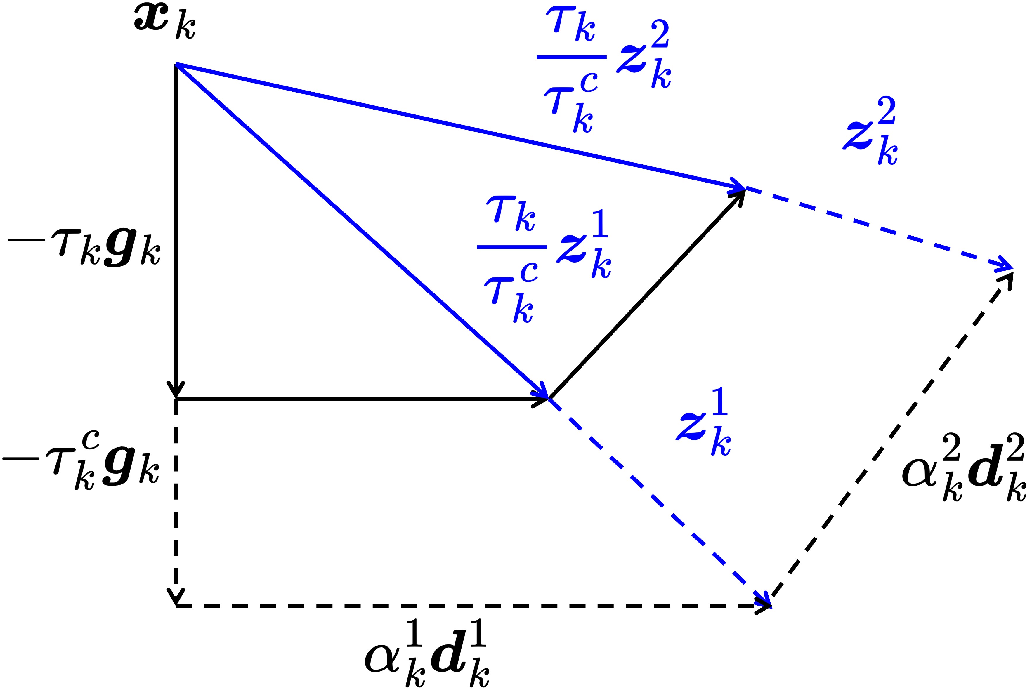
Given a , we find
| (12) |
for certain by the standard proximal operator and certify as a descent direction if . We apply the majorization test along the CG sequence, accepting the last direction that passes and recording the first that fails; the latter typically offers a closer Krylov-subspace approximation to the Newton step. These two directions then serve as endpoints for the subsequent segment backtracking. We summarize the whole algorithm in the following:
Line 5 tests the latest CG direction(s) from Line 3 and continues the CG update if the majorization condition holds. Line 5 is well defined and always identifies a direction that satisfies the majorization condition. In the worst case, setting and choosing reduces (11) to (2). Since is selected to satisfy (4), this case guarantees majorization. PCG is Hessian-free: Hessian–vector products are obtained via automatic differentiation without forming . For any vector , In practice, one first evaluates and then differentiates with respect to . See [31, Ch. 8.4] for details. We also provide the global convergence result for Algorithm 1.
Theorem 1.
Let be a sequence generated by Algorithm 1. Then every accumulation point of is a critical point of .
Proof.
Due to space limitations, we sketch the main arguments. We show that the sequence is nonincreasing and convergent and , where . With these two arguments, adapting the proof template in [18, 32, 33] then yields the theorem. By the majorization principle and optimality of proximal operator, we have and . Combining two together gets which implies . Since is coercive and lsc thus lower bounded, we can conclude the is convergent and the sequence is bounded. Denote and as the accumulation point of and the corresponding function value, respectively. Summing over gives . Because is bounded and , the weights are bounded below by a positive constant; hence as . ∎
4 Numerical Results
We compare PCG with PG [16], its extrapolated variant APG [18], PANOC [24], and ZeroFPR [25]. These methods are chosen because they avoid explicit matrix inversion, which is prohibitive at our problem scales. All experiments were conducted in Julia on a Windows 11 laptop with an Intel Core i7-11800H CPU and 32 GB of RAM.


Compressed sensing MRI: CS-MRI reconstructs images from undersampled k-space by exploiting wavelet transform sparsity. We use the SCAD penalty as the sparsity regularizer (definition in [4]). The optimization formulation is
where is the sampling mask, denotes the 2-D FFT, is the measured k-space data, and is the 2-D wavelet transform. Since denotes an orthonormal transform, the proximal operator of can be computed as . Following [34], for each component ,
with thresholds and . Because the Hessian of is an orthogonal projector with spectrum , the inner CG loop converges rapidly. Matrix-vector products reduce to (2-D) FFTs, further lowering cost. We evaluate all methods on a grayscale brain MRI image [35]. Cartesian -space is undersampled using a variable-density Bernoulli pattern with a fully sampled central disk ( of the radius). Outside the center, samples are drawn independently with probability . Gaussian noise is added to achieve . The regularization parameter was set as and . The simulation results are shown in Figure 2. Our method converges faster than competing methods in both iteration count and computing time. With the same initialization, it also attains a slightly higher PSNR.


Dictionary Learning: We next consider a bilinear inverse problem, where the data-fidelity term is nonconvex. A prototypical case is dictionary learning [36, 37]:
where , , and . Here denotes the indicator of a set , i.e., if and otherwise. Thus enforces unit-norm atoms and enforces at-most- sparsity per code column. Its proximal operator decouples columnwise: it projects by normalizing each atom to unit norm and projects by keeping, in each column, the largest-magnitude entries and zeroing the rest. is randomly generated Gaussian matrix with unit norm columns. Each column of contains non-zeros with uniformly random support and i.i.d. standard-Gaussian values. We consider , , , and . Figure 3 illustrates that our method achieves lower reconstruction error with fewer iterations and reduced runtime. It also avoids the late-iteration variable oscillations observed in competing methods.
5 Conclusions
This paper develops a proximal CG method for nonconvex nonsmooth optimization. Leveraging CG iterates, we estimate a stepsize via the Lanczos process and choose a descent direction via a tailored majorization strategy. Numerical results on image processing and bilinear inverse problems show fast convergence, low computational cost, and strong reconstruction quality.
References
- [1] Michael Ting, Raviv Raich and Alfred Hero “Sparse image reconstruction for molecular imaging” In IEEE Transactions on Image Processing 18.6 IEEE, 2009, pp. 1215–1227
- [2] Hui Zou “The adaptive lasso and its oracle properties” In Journal of the American statistical association 101.476 Taylor & Francis, 2006, pp. 1418–1429
- [3] Felix Abramovich and Vadim Grinshtein “High-dimensional classification by sparse logistic regression” In IEEE Transactions on Information Theory 65.5 IEEE, 2018, pp. 3068–3079
- [4] Jianqing Fan and Runze Li “Variable selection via nonconcave penalized likelihood and its oracle properties” In Journal of the American statistical Association 96.456 Taylor & Francis, 2001, pp. 1348–1360
- [5] Thomas Blumensath and Mike Davies “Iterative hard thresholding for compressed sensing” In Applied and computational harmonic analysis 27.3 Elsevier, 2009, pp. 265–274
- [6] Cun-Hui Zhang “Nearly unbiased variable selection under minimax concave penalty”, 2010
- [7] Yuejie Chi, Yue Lu and Yuxin Chen “Nonconvex optimization meets low-rank matrix factorization: An overview” In IEEE Transactions on Signal Processing 67.20 IEEE, 2019, pp. 5239–5269
- [8] Wei Dai, Ely Kerman and Olgica Milenkovic “A geometric approach to low-rank matrix completion” In IEEE Transactions on Information Theory 58.1 IEEE, 2012, pp. 237–247
- [9] Yiming Zhou, Huayu Fu and Wei Dai “Efficient Gridless Wideband Direction-of-Arrival Estimation From Many Frequencies” In ICASSP 2025-2025 IEEE International Conference on Acoustics, Speech and Signal Processing (ICASSP), 2025, pp. 1–5 IEEE
- [10] Xi Yao and Wei Dai “A Low-rank Projected Proximal Gradient Method for Spectral Compressed Sensing” In IEEE Transactions on Signal Processing IEEE, 2025
- [11] Benjamin Recht, Maryam Fazel and Pablo Parrilo “Guaranteed minimum-rank solutions of linear matrix equations via nuclear norm minimization” In SIAM review 52.3 SIAM, 2010, pp. 471–501
- [12] Jared Tanner and Ke Wei “Normalized iterative hard thresholding for matrix completion” In SIAM Journal on Scientific Computing 35.5 SIAM, 2013, pp. S104–S125
- [13] Xiao Li, Qi Liu and Hing So “Rank-one matrix approximation with lp-norm for image inpainting” In IEEE Signal Processing Letters 27 IEEE, 2020, pp. 680–684
- [14] Daniel Lee and H Seung “Algorithms for non-negative matrix factorization” In Advances in neural information processing systems 13, 2000
- [15] Ivana Tošić and Pascal Frossard “Dictionary learning” In IEEE Signal Processing Magazine 28.2 IEEE, 2011, pp. 27–38
- [16] Patrick Combettes and Jean-Christophe Pesquet “Proximal splitting methods in signal processing” In Fixed-point algorithms for inverse problems in science and engineering Springer, 2011, pp. 185–212
- [17] Amir Beck “First-order methods in optimization” SIAM, 2017
- [18] Huan Li and Zhouchen Lin “Accelerated proximal gradient methods for nonconvex programming” In Advances in neural information processing systems 28, 2015
- [19] Jason Lee, Yuekai Sun and Michael Saunders “Proximal Newton-type methods for minimizing composite functions” In SIAM Journal on Optimization 24.3 SIAM, 2014, pp. 1420–1443
- [20] Man-Chung Yue, Zirui Zhou and Anthony-Cho So “A family of inexact SQA methods for non-smooth convex minimization with provable convergence guarantees based on the Luo–Tseng error bound property” In Mathematical Programming 174.1 Springer, 2019, pp. 327–358
- [21] Christian Kanzow and Theresa Lechner “Globalized inexact proximal Newton-type methods for nonconvex composite functions” In Computational Optimization and Applications 78.2 Springer, 2021, pp. 377–410
- [22] Yiming Zhou and Wei Dai “Proximal dogleg opportunistic majorization for nonconvex and nonsmooth optimization” In arXiv preprint arXiv:2402.19176, 2024
- [23] Lorenzo Stella, Andreas Themelis and Panagiotis Patrinos “Forward–backward quasi-Newton methods for nonsmooth optimization problems” In Computational Optimization and Applications 67.3 Springer, 2017, pp. 443–487
- [24] Lorenzo Stella, Andreas Themelis, Pantelis Sopasakis and Panagiotis Patrinos “A simple and efficient algorithm for nonlinear model predictive control” In 2017 IEEE 56th Annual Conference on Decision and Control (CDC), 2017, pp. 1939–1944 IEEE
- [25] Andreas Themelis, Lorenzo Stella and Panagiotis Patrinos “Forward-backward envelope for the sum of two nonconvex functions: Further properties and nonmonotone linesearch algorithms” In SIAM Journal on Optimization 28.3 SIAM, 2018, pp. 2274–2303
- [26] Yu Nesterov “Gradient methods for minimizing composite functions” In Mathematical programming 140.1 Springer, 2013, pp. 125–161
- [27] Jorge Nocedal and Stephen Wright “Numerical optimization” Springer, 2006
- [28] Ruyu Liu, Shaohua Pan, Yuqia Wu and Xiaoqi Yang “An inexact regularized proximal Newton method for nonconvex and nonsmooth optimization” In Computational Optimization and Applications 88.2 Springer, 2024, pp. 603–641
- [29] Robert Baraldi and Drew Kouri “A proximal trust-region method for nonsmooth optimization with inexact function and gradient evaluations” In Mathematical Programming 201.1 Springer, 2023, pp. 559–598
- [30] Jörg Liesen and Zdenek Strakos “Krylov subspace methods: principles and analysis” Numerical MathematicsScientific Computing, 2013
- [31] Paige Bright, Alan Edelman and Steven Johnson “Matrix Calculus (for Machine Learning and Beyond)” In arXiv preprint arXiv:2501.14787, 2025
- [32] Qunwei Li, Yi Zhou, Yingbin Liang and Pramod Varshney “Convergence analysis of proximal gradient with momentum for nonconvex optimization” In International Conference on Machine Learning, 2017, pp. 2111–2119 PMLR
- [33] Pierre Frankel, Guillaume Garrigos and Juan Peypouquet “Splitting methods with variable metric for Kurdyka–Łojasiewicz functions and general convergence rates” In Journal of Optimization Theory and Applications 165.3 Springer, 2015, pp. 874–900
- [34] Patrick Breheny and Jian Huang “Coordinate descent algorithms for nonconvex penalized regression, with applications to biological feature selection” In The annals of applied statistics 5.1, 2011, pp. 232
- [35] ImageJ, National Institutes of Health “MRI Stack (sample image)” Public domain, https://imagej.net/ij/images/mri-stack.zip, n.d.
- [36] Michal Aharon, Michael Elad and Alfred Bruckstein “K-SVD: An algorithm for designing overcomplete dictionaries for sparse representation” In IEEE Transactions on signal processing 54.11 IEEE, 2006, pp. 4311–4322
- [37] Wei Dai, Tao Xu and Wenwu Wang “Simultaneous codeword optimization (SimCO) for dictionary update and learning” In IEEE Transactions on Signal Processing 60.12 IEEE, 2012, pp. 6340–6353