A tree-based kernel for densities and its applications in clustering DNase-seq profiles

Abstract

Modeling multiple sampling densities within a hierarchical framework enables borrowing of information across samples. These “density random effects” can act as kernels in latent variable models to represent exchangeable subgroups or clusters. A key feature of these kernels is the (functional) covariance they induce, which determines how densities are grouped in mixture models. Our motivating problem is clustering chromatin accessibility profiles from high-throughput DNase-seq experiments to detect transcription factor (TF) binding. TF binding typically produces footprint profiles with spatial patterns, creating long-range dependency across genomic locations. Existing nonparametric hierarchical models impose restrictive covariance assumptions and cannot accommodate such dependencies, often leading to biologically uninformative clusters. We propose a nonparametric density kernel flexible enough to capture diverse covariance structures and adaptive to various spatial patterns of TF footprints. The kernel specifies dyadic tree splitting probabilities via a multivariate logit-normal model with a sparse precision matrix. Bayesian inference for latent variable models using this kernel is implemented through Gibbs sampling with Pólya–Gamma augmentation. Extensive simulations show that our kernel substantially improves clustering accuracy. We apply the proposed mixture model to DNase-seq data from the ENCODE project, which results in biologically meaningful clusters corresponding to binding events of two common TFs.

Keywords: Bayesian inference; nonparametric models; latent variable models; hierarchical models; tree-based models.

1 Introduction

Many modern biomedical applications require modeling multiple unknown groups, each consisting of i.i.d. observations drawn from a group-specific unknown distribution. In particular, we focus on the count data in the form of $\mathbf{X}\in\mathbb{N}_{0}^{n\times p}$ (see Figure S3), where each row is a $p$-dimensional count vector, representing one observation that belongs to an unknown latent group. Such $p$-dimensional random vectors are often assumed to be exchangeable, and $n$ such vectors can be modeled as a mixture of several (group-specific) distributions. Count data exists ubiquitously in biological applications using various sequencing technologies: each $p$-dimensional random vector records the count of sequenced fragments assigned to $p$ genomic, taxonomic, or other biological features. For example, in DNase-seq data, the vector records fragment counts across genomic positions around a candidate regulatory site; in microbiome sequencing data, it records counts of DNA or RNA reads assigned to different taxa. There are several statistical challenges in clustering such count profiles. The count vectors are usually high-dimensional, overdispersed, and exhibit complex correlation structures driven by biological and spatial factors. Observations of the count vectors often show different distributional patterns across different subgroups, and this forms the basis for differentiating clusters.

A brief review on clustering count data. A variety of methods have been proposed for clustering count vectors. Popular distance-based methods, such as K-means and Partitioning Around Medoids (PAM), cluster observations based on geometric dissimilarity, but do not explicitly account for the complex dependence and overdispersion often present in count data. Model-based approaches provide a more principled alternative by introducing cluster-specific sampling distributions, with either parametric or nonparametric kernels.

Among model-based methods, Holmes et al. (2012) adopted a mixture of Dirichlet kernels for each cluster, which assumes that, within a cluster, the counts across the elements in the vector are independent up to a total-sum constraint. Extending the vector to possibly involve an infinite number of elements, the nested Dirichlet Process (NDP) (Rodriguez et al., 2008) also adopts a mixture model of the Dirichlet kernel, but assumes no heterogeneity within each cluster. Christensen and Ma (2020) and Mao and Ma (2022) considered a mixture model with a finite Pólya tree kernel (Ferguson, 1973; Lavine, 1992; Dennis III, 1991), which allows within-cluster heterogeneity but the within-cluster correlation across different elements in the count vector is prespecified by the dyadic tree structure rather than learned adaptively from the data. More recent works have proposed mixture of DP mixtures (Zhang et al., 2026) with a fixed number of groups, and a covariate-dependent tail-free process (Flores and Müller, 2025) to utilize covariate information in clustering.

Closely related to our work is the broader literature on hierarchical modeling of exchangeable random distributions. Extending the classical Gaussian hierarchical paradigm, Bayesian nonparametric hierarchical models allow both observation-level and population-level distributions to lie in much richer families. Examples include the hierarchical Dirichlet process (Teh et al., 2006), hierarchical Pitman-Yor processes (Teh, 2006; Camerlenghi et al., 2017), to more recent hierarchical normalized completely random measures (Argiento et al., 2020), and hierarchical Pólya tree (Christensen and Ma, 2020). While these models have large marginal support for each observation-level distribution, they all impose very restrictive constraints on the variation among the observation-level distribution due to the small number of parameters they devote to characterizing such functional covariance.

DNase-seq data as one motivating example. DNase-seq is a high-throughput assay for measuring chromatin accessibility. The DNase I enzyme preferentially cuts accessible genomic regions that are not tightly bound by nucleosomes or other proteins, such as transcription factors. After sequencing and aligning the resulting fragments, one can identify regions with high cleavage intensity, known as DNase I hypersensitive sites (DHSs), which are often enriched for regulatory elements, including promoters, enhancers, and Transcription Factor (TF) binding sites (Consortium and others, 2012).

In our application, the observational units are candidate TF binding sites. Each site is represented by a count profile across genomic positions in a window around the motif match. Within accessible chromatin, TF binding can protect local DNA from DNase I cleavage, producing characteristic footprints (Figure S3): lower read counts in the motif region and higher counts in the flanking regions, exhibiting a bimodal shape. Clustering such DNase-seq count profiles can therefore help distinguish different patterns of TF binding and improve the identification of bound versus unbound sites. This application also illustrates the statistical challenges of count-data clustering. The count vectors are high-dimensional, overdispersed, and spatially dependent across nearby genomic positions, while substantial heterogeneity may still exist within each cluster among observation-level count vectors. An effective clustering method must therefore incorporate both cross-group and within-group variation while accounting for dependence across the support.

Several methods have been developed specifically for identifying TF binding sites using DNase-seq data. These include site-centric approaches such as early k-means-based methods (Boyle et al., 2011), covariate-assisted mixture models such as CENTIPEDE (Pique-Regi et al., 2011), PIQ (Sherwood et al., 2014), and segmentation-based methods such as Gusmao et al. (2014). While useful in this domain, these methods rely on DNase-seq-specific assumptions or auxiliary information, which makes them less transferable to more general count-data clustering problems, such as the microbiome count data.

Our contribution. In this paper, we propose a general-purpose mixture model for clustering count vectors with flexible within-cluster covariance, allowing the correlation pattern within each cluster to adapt to the data through a Bayesian prior on the covariance structure. We develop an efficient sampling algorithm with R package implementation, and demonstrate its advantages in both simulated and real data. We apply the model to the Encyclopedia of DNA Elements (ENCODE) Consortium (Consortium and others, 2012) DNase-seq data to cluster TF footprints, where it achieves improved accuracy relative to benchmark methods and aligns with the reference biological truth validated by the ChIP data. An extension to the microbiome data of the proposed method, featuring a phylogenetic tree structure, is applied to the American Gut Project (McDonald et al., 2018) data in Supplementary Section S4.1.

Organization. Section 2 introduces our proposed correlated tree model and its theoretical properties. Section 3 provides details on the sampling algorithm. Section 4 provides numerical evidence of the superior performance of our proposed methods based on simulation studies. Section 5 gives the biological background of the DNase-seq data and the numerical comparison of our method with the competing methods and reference truth. We conclude with a discussion on the potential extensions and limitations in Section 6.

2 A tree-based sampling model for count histograms with flexible covariance

Our proposed sampling model is based on recursive dyadic partitioning of the sample space. At each split, the probability mass is divided between two child nodes, parameterized by the conditional splitting probabilities. We model the conditional splitting probabilities with a prior that accounts for the spatial correlation.

2.1 The dyadic tree specification of probability distributions

We begin with a brief introduction to a tree-based parameterization of a probability distribution. This parameterization has been used in both Bayesian (Ferguson, 1973; Lavine, 1992) and non-Bayesian (Dennis III, 1991) literature to model probability distributions. We will later use this parameterization to construct a new model.

Visualized in Figure 1(a), we consider a constructive process in which a probability distribution $P$ can be described through sequential splitting of the unit mass along a dyadic partition tree on the sample space $\mathfrak{X}$. Let $\mathcal{T}_{0}=\left\{\mathfrak{X}\right\}$, $\mathcal{T}_{1}=\left\{A_{0},A_{1}\right\}$, $\mathcal{T}_{2}=\left\{A_{00},\dots,A_{11}\right\}$, and so on. Here, we adopt the binary notations in Chapter 3 Section 3.5 in Ghosal and Van der Vaart (2017). Let $l$ be the layer index, $\mathcal{T}_{l}$ is the $l$-th layer partition consisting of $2^{l}$ nodes. Each node in $\mathcal{T}_{l}$ is indexed by a string $\epsilon=\epsilon_{1}\cdots\epsilon_{l}$, a length $l$ sequence of 0s and 1s, indicating whether it is a left ($\epsilon_{l}=0$) or right ($\epsilon_{l}=1$) child in each step of the tree split. Let $\mathcal{E}=\left\{0,1\right\}$, $\mathcal{E}^{l}$ the collection of strings $\epsilon_{1}\dots\epsilon_{l}$ of length $l$, which is the index set for $\mathcal{T}_{l}$, and $\mathcal{E}^{*}=\cup_{l=0}^{\infty}\mathcal{E}^{l}$. In each split, $A_{\epsilon}=A_{\epsilon 0}\cup A_{\epsilon 1}$ and $A_{\epsilon 0}\cap A_{\epsilon 1}=\emptyset$, and a probability measure $P$ would satisfy $P(A_{\epsilon})=P(A_{\epsilon 0})+P(A_{\epsilon 1})$. The probability mass splits according to the conditional probabilities $V_{\epsilon 0}=P(A_{\epsilon 0}|A_{\epsilon})$, and $V_{\epsilon 1}=P(A_{\epsilon 1}|A_{\epsilon})=1-V_{\epsilon 0}$. The probability mass on any node $\epsilon=\epsilon_{1}\dots\epsilon_{l}\in\mathcal{E}^{l}$ in this dyadic tree can be recovered by $P(A_{\epsilon_{1}\cdots A_{\epsilon_{l}}})=\prod_{j=1}^{l}V_{\epsilon_{1}\dots\epsilon_{j}}$. Figure 2(a) provides the visualization of this dyadic partitioning process in a numeric example for two different distributions supported on $[0,1]$. The top row is one sample drawn from a mixture of two beta distributions with different modes, and the bottom row is another sample drawn from a distribution with one mode.

Figure 2(a) illustrates the recursive partitioning process. At each level $l$, the probability distribution $P$ is approximated by a multinomial probability vector of length $2^{l}$. If a sample $X_{1}^{P},\dots,X_{n}^{P}$ is drawn from an unknown distribution $P$, we can partition the sample space $\mathfrak{X}$ by the aforementioned way and count how many $X_{i}^{P}$ fall into each set $A_{\epsilon}$, denoting $n_{p}(A_{\epsilon})=\sum_{i=1}^{n}I(X^{P}_{i}\in A_{\epsilon})$. The empirical conditional splitting probability is $\widehat{V}_{\epsilon 0}=\frac{n_{p}(A_{\epsilon 0})}{n_{p}(A_{\epsilon})}$.

(a) Dyadic Partitioning Tree

(b) A tree-based sampling model with hyperpriors on mean and covariance

Figure 1: Graphical Illustration of CorTree

2.2 The hierarchical tree model with sparse covariance structure

Let $X^{i}_{[m_{i}]}=\left\{X^{i}_{1},\dots,X^{i}_{m_{i}}\right\}$ be the $i$-th sample with $m_{i}$ independent draws from an underlying distribution $Q_{i}$. Within each subgroup, the individual densities $Q_{i}$ are assumed to independently follow the same underlying sampling distribution, in our case, the correlated tree distribution. In the observed count data, we only have count vectors of $\mathbf{X}_{i}=\left\{X_{i}(B_{1}),\dots,X_{i}(B_{p})\right\}$ where $B_{1},\dots,B_{p}$ are the histogram partition bins, and $X_{i}(B_{j})=\sum_{k=1}^{m_{i}}I(X^{i}_{k}\in B_{j})$. With $n$ independent samples, the observed count matrix is $\mathbf{X}=\left(\mathbf{X}_{1},\dots,\mathbf{X}_{n}\right)^{\mathrm{T}}\in\mathbb{R}^{n\times p}$. In practice, $B_{1},\dots,B_{p}$ are not necessarily the same as the tree leaf nodes, since we use the dyadic partition, and $p$ might not be exactly $2^{l}$, in which case we usually choose the number of layers $l$ so that $2^{l}$ is larger than $p$. In this work, to incorporate the spatial structure, we propose a hierarchical tree model with a sparse covariance structure. The hierarchical structure is illustrated in Figure 1(b), where $Q_{i}$ is represented by a tree-structured density learner defined below.

Definition 1 formally defines a nonparametric tree model indexed by the transformed splitting probabilities $\bm{\psi}=\left\{\psi_{\epsilon},\epsilon\in\mathcal{E}^{*}\right\}$. Let $\text{logit}(p):=\log(\frac{p}{1-p})$, and $\text{logit}^{-1}(\psi)=1/(1+\exp^{-\psi})$.

Definition 1 (Dyadic Tree with parameter $\bm{\psi}$).

Given the sample space $\mathfrak{X}$ and a dyadic partition sequence $\{\mathcal{T}_{l}\}_{l=0}^{\infty}$, let $\psi_{\varepsilon}=\text{logit}(V_{\varepsilon})$. Then we say that $X$ follows a Dyadic Tree distribution with parameter $\bm{\psi}$ and write $X\sim\mathrm{Tree}(\bm{\psi})$ if starting from $\epsilon=\emptyset$, $X(A_{\epsilon 0})\sim\mathrm{Bin}\left\{X(A_{\epsilon}),\text{logit}^{-1}(\psi_{\epsilon 0})\right\}$ for all $\epsilon$.

Our main strategy for incorporating spatial correlation is to transform the conditional splitting probability $V_{\epsilon 0}$ to the real line by the logit transform $\psi_{\epsilon}=\text{logit}(V_{\epsilon})$ (Jara and Hanson, 2011), and assign a multivariate normal distribution on the vectorized $\psi_{\epsilon}$ across different locations $A_{\epsilon}$. The logit transform in Definition 1 enables us to define a tree model with a covariance structure. Let $I_{c}\subset\mathcal{E}^{*}$ be the index set of all correlated splitting probabilities. For computational convenience, we let the first $L$ layers of splitting probabilities be correlated. Because $V_{\epsilon 1}=1-V_{\epsilon 0}$, only including the left splitting probabilities in $I_{c}$ is sufficient. Hence $|I_{c}|=\sum_{l=1}^{L}2^{l-1}=2^{L}-1$.

Definition 2 (Fixed-layer Correlated Tree).

$\bm{\psi}$ is said to have a Fixed-layer Correlated Tree distribution if for a fixed integer $L>0$, $\bm{\psi}_{L}=\left\{\psi_{\epsilon}:\epsilon\in I_{c}\right\}\in\mathbb{R}^{2^{L}-1}$,

$$\bm{\psi}_{L} \sim N(\bm{\mu},\bm{\Sigma}),$$

$$\psi_{\epsilon} \overset{\scriptsize\mbox{ind}}{\sim}N(\mu_{\epsilon},\sigma^{2}_{\epsilon}),\quad\epsilon\in\mathcal{E}^{*}\backslash I_{c}.$$ (1)

Let $\bm{\tau}=\left\{\mu_{\epsilon},\sigma^{2}_{\epsilon}\right\}_{\epsilon\in\mathcal{E}^{*}\backslash I_{c}}$ be the collection of parameters in the independent tail splitting variables. Denote $\bm{\psi}\sim\text{CorT}(\bm{\mu},\bm{\Sigma},\bm{\tau};L)$ as the correlated tree prior specified in (1).

This definition applies to both trees of a finite maximal depth or an infinitely deep tree. We assume that beyond level $L$, the tail probabilities $\psi_{\epsilon}$ are independent for $\epsilon\in\mathcal{E}^{*}\backslash I_{c}$, and $\mu_{\epsilon}$ and $\sigma_{\epsilon}^{2}$ both decay to 0 as the layer goes deeper, making the tail splitting variable $\psi_{\epsilon}$ shrink to 0 in the deeper tree nodes. We assign hyperpriors $\sigma_{\epsilon}^{2}\sim\mathrm{InvGamma}(c,1/l_{\epsilon})$ where $l_{\epsilon}$ is the layer of $\epsilon$, $l_{\epsilon}=\lfloor\log_{2}\epsilon\rfloor$, $c$ is an adjustable hyperparameter, default at 1. Similarly, $\mu_{\epsilon}\sim N(0,\sigma_{\mu}^{2})$ where $\sigma_{\mu}^{2}$ is allowed to decay to 0 for deeper layers. In practice, when we only have a finite tree, $\sigma_{\mu}^{2}$ is set to be a small number.

Such a distribution with finite layers of correlated structure, as in Definition 2, can be used to model both finite histograms and absolute continuous distributions with respect to a base measure $\lambda$ such as the Lebesgue measure on $\mathfrak{X}=[0,1]$. In the latter case, it has a large support that includes all absolutely continuous measures with respect to $\lambda$. This allows the models to be applied to continuous sampling distributions as well as finite histograms. While in principle, all real data are discretized at some level (e.g., up to the precision of the measurements or recording), it is helpful to have a sampling distribution supported on density functions that can accommodate long-range dependency such as those induced to symmetry.

Proposition 1.

If $P$ is a random measure with transformed splitting variables $\left\{\psi_{\epsilon},\epsilon\in\mathcal{E}^{*}\right\}$ that follow Definition 2, and assume that for the tail splitting variables, $|\mu_{\epsilon}|\leq\delta_{l}$ and $\sigma_{\epsilon}^{2}\leq\gamma_{l}$ for any $\epsilon\in\mathcal{E}^{l}$ where $l>L$, such that $\sum_{l}(\delta_{l}+\gamma_{l})<\infty$, then almost all realizations of $P$ are absolutely continuous with respect to $\lambda$. In addition, the total variational support of $P$ consists of all probability measures that are absolutely continuous with respect to $\lambda$.

Proof (Supplementary Section S1) of this Proposition directly follows by checking the conditions of Theorem 3.16 and Theorem 3.19 in Ghosal and Van der Vaart (2017). The absolute continuity result in Proposition 1 guarantees that realizations of such random measures can form a density. If the splitting variables divide the mass unevenly (i.e., $\mu_{\epsilon}$ is away from 0), the resulting realizations may concentrate around some points rather than forming a density. Proposition 1 also ensures that our prior has full support over the space of probability measures that are absolutely continuous w.r.t. the base measure $\lambda$. Both of the results are properties of a tail-free process. A tail-free process is defined as $\left\{V_{\epsilon 0}:\epsilon\in\mathcal{E}^{l}\right\}\perp\left\{V_{\epsilon 0}:\epsilon\in\mathcal{E}^{l^{\prime}}\right\}$ when $l\neq l^{\prime}$, meaning that the splitting variables across different layers are independent of each other. Our proposed prior in Definition 2 benefits from the good theoretical properties of a tail-free process by having a finite number of layers with correlated splitting variables and an infinite sequence of independent tail splitting variables.

For the mean and covariance of the correlated splitting variables $\bm{\psi}_{L}\sim N(\bm{\mu},\bm{\Sigma})$, we let $\pi_{\mu}$ be $N(0,\sigma_{\mu}^{2}\bm{I})$ and assume that $G$ is a sparse covariance. One convenient model that induces such sparsity in the covariance is the Graphical Horseshoe (GHS) Prior for which there exists simple computational recipes. (See details in Section 3.)

Lastly, for clustering the samples based on their underlying sampling densities, we consider a Dirichlet process mixture (DPM) model with the correlated tree kernel. While one can describe a DPM in several equivalent ways, here we describe it using its stick-breaking representation (Sethuraman, 1994). In the model, $Z_{i}$ is a latent cluster membership variable for observation $i$.

Definition 3 (Dirichlet process mixture of correlated trees).

For $i=1,\dots,n$,

$$X_{i}|Z_{i}=k,\bm{\psi}_{i}^{(k)} \sim\mathrm{Tree}(\bm{\psi}_{i}^{(k)}),$$

$$\bm{\psi}_{i}^{(k)}|Z_{i}=k \sim\text{CorT}(\bm{\mu}^{(k)},\bm{\Sigma}^{(k)},\bm{\tau}^{(k)};L),\quad k=1,2,\dots,$$

$$Z_{i}\,|\,\pi \sim{\rm MultiBern}(\infty,\pi),\quad\pi\sim\mathrm{GEM}(\alpha),$$ (2)

where $\mathrm{GEM}(\alpha)$ is the Griffiths-Engen-McCloskey stick-breaking model that induces the Dirchlet process with concentration parameter $\alpha$ (Sethuraman, 1994) and MultiBern($\infty,\pi)$ represents the “infinity multinomial-Bernoulli”, i.e., the discrete distribution with probability $\pi_{k}$ on the value $k$. Specifically, $\pi_{k}=\beta_{k}\prod_{b=1}^{k}(1-\beta_{b}),\beta_{k}\sim\text{Beta}(1,\alpha)$. The superscript $(k)$ in $\bm{\psi}^{(k)},\bm{\mu}^{(k)},\bm{\Sigma}^{(k)},\bm{\tau}^{(k)}$ indicates cluster-specific parameters. We refer to the hierarchical model (2) as the Clustering Correlated Tree.

Now, we have a correlated tree distribution that (i) incorporates the spatial correlation, (ii) is supported on a large class of absolutely continuous distributions, and (iii) can be adopted as a distributional kernel in mixture models for clustering. We next turn to computational strategies for posterior sampling under this model.

3 Computation

We implement the Dirichlet process mixture of correlated trees model using a Gibbs sampler, and the R package CorTree is written using RcppArmadillo (Eddelbuettel and Sanderson, 2014) and is available on https://github.com/yuliangxu/CorTree. The posterior sampling of $\bm{\psi}$ uses the Pólya-Gamma augmentation (Polson et al., 2013). This allows us to have fully conjugate posteriors on $\bm{\psi}$. The detailed posterior derivation can be found in the Supplementary Section S2.

In Section 2, the prior on the latent covariance $\bm{\Sigma}$ can be any general sparse covariance prior. The sparse covariance prior is a family of distributions that has support on the symmetric and semi-definite matrices and also induces sparsity on the off-diagonal elements. There are also frequentist alternatives of estimating the precision matrix using graphical lasso (Friedman et al., 2008) and the smoothly clipped absolute deviation (SCAD) penalty (Fan and Li, 2001). Such Bayesian priors include the graphical lasso prior (Wang, 2012) and the Graphical Horseshoe (GHS) prior (Li et al., 2019). Here, we choose the most recent state-of-the-art sparse covariance prior, the Graphical Horseshoe prior, which has been shown in Li et al. (2019) to have superior performance in identifying nonzero pairs.

The GHS prior is placed on the precision matrix $\bm{\Omega}=\bm{\Sigma}^{-1}\in\mathcal{S}_{L}$ where $S_{L}$ is the space of $L\times L$ positive definite matrices. Let $i,j=1,\dots,L$, the GHS prior is defined by assigning horseshoe priors on the off-diagonal elements

$$\omega_{ii} \propto 1,\quad\omega_{ij:i<j}\sim N(0,\lambda_{ij}^{2}\tau^{2}),\quad\lambda_{ij}\sim C^{+}(0,1),\quad\tau\sim C^{+}(0,1),$$

where $C^{+}(0,1)$ is the half-Cauchy distribution. The prior on $\bm{\Omega}$ can be written as

$$p(\bm{\Omega}|\tau)\propto\prod_{i<j}N(\omega_{ij}|\lambda^{2}_{ij},\tau^{2})\prod_{i<j}C^{+}(\lambda_{ij}|0,1)1_{\bm{\Omega}\in\mathcal{S}_{L}}.$$

Algorithm 1 in (Li et al., 2019) provides the fully conjugate update of all posteriors. We provide a C++ implementation for Algorithm 1 in our package based on the MATLAB implementation from the original paper Li et al. (2019).

(a) Recursive partition of the sample space via dyadic tree structure for two different densities.

(b) Density plot for the simulated two groups of samples. The green group with two modes (dashed-line boxed) is designed to mimic the transcription factor (TF) “footprint” pattern.

Figure 2: Illustration of the simulated data example.

4 Simulation Study

We design a simulation study to compare the clustering performance of CorTree with the following competing methods: (i) K-means (Forgy, 1965); (ii) Partitioning Around Medoids (PAM), implemented in R package cluster (Maechler et al., 2024), (iii) independent tree (IndTree), and (iv) Dirichlet Multinomial Mixture (DMM) (Holmes et al., 2012). The comparison among DMM, IndTree, and CorTree can be seen as an ablation study shown in Figure S2: IndTree incorporates the within-cluster heterogeneity among different observations, and CorTree allows the second moment structure of such within-cluster heterogeneity to be adaptively learned from the data.

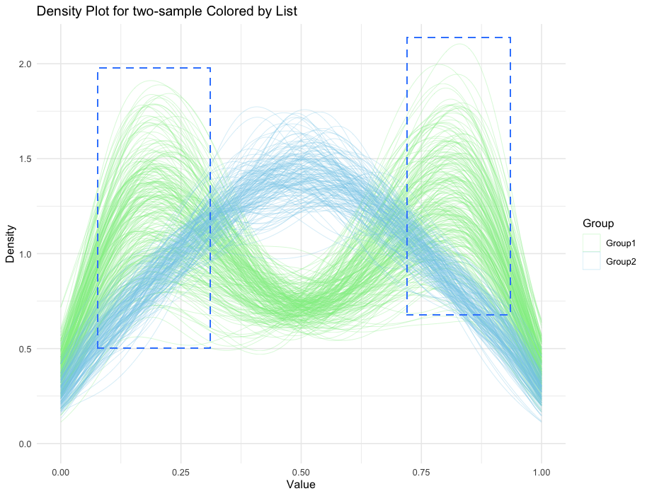
We simulate $X_{[m_{j}]}^{j}\overset{\scriptsize\mbox{iid}}{\sim}Q_{j}$, where $Q_{j}$ is sampled from a mixture of the following two groups of samples (shown in Figure 2(b)).

$$\text{Group 1: }Q_{j} \sim W_{j}\times\text{Beta}(2,6)+(1-W_{j})\times\text{Beta}(6,2),\quad W_{j}\sim\text{Beta}(10,10);$$

$$\text{Group 2: }Q_{j} \sim W_{j}\times\text{Beta}(1,1)+(1-W_{j})\times\text{Beta}(3,3),\quad W_{j}\sim\text{Beta}(10,10).$$

Group 1 (green lines in Figure 2(b)) is a bi-modal distribution with two modes at $1/4$ and $3/4$ within the support $[0,1]$, mimicking the transcription factor (TF) “footprint” pattern in the DNase-Seq data, with a dip in the middle motif region and higher numbers in the flanking regions around the motif (the two modes as dashed lines boxed in Figure 2(b)). Group 2 (blue lines in Figure 2(b)) is generated as a unimodal distribution. For each density $Q_{j}$, we sample $X_{[m_{j}]}^{j}\overset{\scriptsize\mbox{iid}}{\sim}Q_{j}$ with $m_{j}$ uniformly sampled from $10^{3}$ to $5\times 10^{3}$. Each $Q_{j}$ is a mixture of two beta distributions, with the mixing probability $W_{j}$ randomly sampled from $\text{Beta}(10,10)$ to represent the within-cluster heterogeneity of $Q_{j}$. Each line in Figure 2(b) represents one observation $Q_{j}$. Some $Q_{j}$ have a higher left mode than the right mode, others vice versa. We generate a total of $n$ observations $Q_{j},j=1,\dots,n$, 60% from cluster 1 and 40% from cluster 2. After generating $X_{[m_{j}]}^{j}$, we compute the histogram of $X_{[m_{j}]}^{j}$ with 1000 bins over $[0,1]$, and use the resulting data as input for clustering algorithms. This gives us $X\in\mathbb{R}^{n\times 1000}$ for each replicated study.

In practice, it is difficult to know a priori how many true clusters exist in the data, and the competing methods all require a prespecified number of clusters. Hence, we set the cluster number to be 3 for all methods, although there are only 2 true clusters. To quantify the clustering accuracy, we use the Adjusted Rand Index (ARI), defined in Halkidi et al. (2002) and implemented in the R package mclust (Scrucca et al., 2023). ARI can handle label permutation and provides the corrected-for-chance version of the Rand index. ARI maps the clustering similarity to $[-1,1]$, with 1 being perfect clustering, 0 being completely random clustering, and -1 being worse than random clustering.

The IndTree and CorTree models are implemented using the Gibbs sampler, and the initial value for the membership variable $Z_{i}$ is set to be the discretized rowsum of $X$. We run 100 MCMC iterations for the burn-in period, and collect the results based on an additional 50 iterations. Both tree models use a 6-layer dyadic tree, and the CorTree model uses the first 4 layers’ splitting variables to be included in the covariance structure, resulting in a covariance matrix of dimension $\mathbb{R}^{31\times 31}$.

Table 1: Clustering results based on 100 replications. Columns report the mean, standard deviation, and median of ARI over 100 replications, the number of times $\mathrm{ARI}=0$ or $\mathrm{ARI}=1$, and the average computation time (in seconds). For each sample, the total count is uniformly drawn between $(10^{3},5\times 10^{3})$.

Experiment	Method	Mean ARI	S.D. ARI	Median ARI	# of ARI=0	# of ARI=1	Avg. time (sec)
$m=200$	K-means	0.30	0.04	0.30	0	0	0.27
	PAM	0.34	0.05	0.34	0	0	0.06
	DMM	0.81	0.15	0.76	0	5	92.60
	IndTree	0.89	0.06	0.89	0	0	220.71
	CorTree	0.94	0.13	1.00	0	76	223.32
$m=400$	K-means	0.30	0.03	0.30	0	0	0.80
	PAM	0.34	0.04	0.34	0	0	0.22
	DMM	0.76	0.15	0.67	0	3	241.62
	IndTree	0.91	0.04	0.91	0	1	441.37
	CorTree	0.96	0.10	1.00	0	83	443.05
$m=600$	K-means	0.30	0.02	0.30	0	0	1.39
	PAM	0.35	0.03	0.35	0	0	0.48
	DMM	0.76	0.15	0.66	0	1	349.57
	IndTree	0.91	0.04	0.91	0	2	657.55
	CorTree	0.96	0.13	1.00	1	86	662.49

Based on the results in Table 1, among all competing methods, CorTree achieves the highest mean and median ARI. DMM, IndTree, and CorTree, in some instances, can achieve perfect clustering (ARI=1). The incrementally flexible design in Figure S2 from DMM, IndTree, to CorTree, leads to increasingly better performance.

5 Clustering of TF footprints using DNase-seq data from ENCODE

Recall Section 1, identifying TF binding sites is critical to understanding gene regulation. We apply CorTree to DNase-seq data from the Encyclopedia of DNA Elements (ENCODE) Consortium (Consortium and others, 2012), with two key TFs, REST (RE1-silencing transcription factor) and NRF1 (Nuclear respiratory factor 1), in the K562 human erythroleukemia cell line. NRF1 maintains cellular energy metabolism and mitochondrial function. REST is a repressor of neuronal gene expression in non-neuronal cells and modulates neurodevelopment.

Since DNase-seq data itself does not contain TF binding specificity information, to define the candidate binding sites for our TFs of interest in our analysis, we scan the genome for TF motif matches. We download position weight matrices (PWMs) from the JASPAR database (Rauluseviciute et al., 2024), scan the human genome for motif matches with REST and NRF1 motifs using FIMO software (Grant et al. (2011)), select motif matches with FIMO p-value $<$ 1e-5 and PWM scores $\geq$ 13, and take 100 bp flanking regions on both sides of the motif matches as the candidate regions of our analysis (Supplementary Section S4 presents analysis without the PWM score preprocessing). We then combine the DNase counts on both strands, and restrict to candidate sites with DNase counts $\geq$ 50 for both REST and NRF1 data. After preprocessing, $\mathbf{X}_{\text{REST}}\in\mathbb{N}_{0}^{4551\times 220}$, with the rowsum ranging from 50 to 9399; $\mathbf{X}_{\text{NRF1}}\in\mathbb{N}_{0}^{8148\times 211}$, with the rowsum ranging from 50 to 22576. To validate the clustering results, we use ChIP-seq data, which has been widely used as a proxy for TF binding truth (Park, 2009). Unlike DNase-seq, ChIP-seq uses an antibody to target a specific TF and therefore provides TF-specific binding measurement. From the ENCODE portal, we obtain normalized ChIP-seq read counts and assign binary labels at the motif match locations that overlap with ChIP-seq peaks. Because ChIP-seq is based on a different experimental technology, we use it only as an independent external reference for validation and method comparison.

We also include a state-of-the-art method tailored for DNase-seq data called CENTIPEDE (Pique-Regi et al., 2011), which uses the continuous PWM score as a site-specific covariate. CENTIPEDE uses a simple mixture of two multinomial components in (3), which clusters sites into 0-1 groups and requires additional site-specific information $Y_{i}$.

$$\mathbf{X}_{i}\in\mathbb{N}_{0}^{p},\mathbf{X}_{i}\sim\pi_{i}\text{Multinomial}(n_{i},\bm{\theta}_{1})+(1-\pi_{i})\text{Multinomial}(n_{i},\bm{\theta}_{0}).\quad\text{logit}(\pi_{i})=Y_{i}^{\mathrm{T}}\beta.$$ (3)

$Y_{i}$ is a 2-dimensional vector, $(1,\text{PWM\_score}_{i})$, to include the intercept term. The unbound sites are simply assumed to be uniformly distributed in CENTIPEDE, which may fail to capture the spatial bias induced by the DNase I enzyme.

Because of the stick-breaking prior for the mixing weights in (2), we need to set a large number of clusters for CorTree to allow the posterior to collapse to fewer clusters. We set 5 clusters for CorTree and IndTree to learn potential subgroup structures, 2 clusters for k-means, PAM, DMM, and CENTIPEDE. Only clusters with more than 10 observations are reported. For CorTree and IndTree, the tree structure is set to 9 layers to have at least one leaf node to represent a single column in $\mathbf{X}$. This dyadic partition leads to many 0s in deeper layers of the tree. We set up to 3 correlated layers for REST data ($\Sigma\in\mathbb{R}^{15\times 15}$), up to 4 correlated layers for NRF1 data ($\Sigma\in\mathbb{R}^{31\times 31}$), collecting 50 MCMC iterations after 100 burn-in iterations (see traceplots in Figure S4). The tuning parameters include the number of correlated layers, the hyperparameter $\alpha_{0}$ in the prior $\sigma_{k,I}^{2}\sim\mathrm{InvGamma}(\alpha_{0},\beta_{0,I})$, and the hyperparameter $\sigma_{\mu}^{2}$ in the hyper-prior $N(0,\sigma_{\mu}^{2})$ for $\mu_{k,C},\mu_{k,I}$. Supplementary Section S4 provides sensitivity analysis for CorTree under varying initial values and hyperparameters.

As a nonparametric clustering method with flexible covariance structure, the posterior of CorTree may have many modes, especially when there are thousands of samples: many distinct cluster configurations can provide similarly good explanations of the data. The choice of the initial $Z$ must be scientifically meaningful to guide meaningful clustering. For the TF binding detection task, the most informative choice is the PWM score, which indicates TF binding specificity, and is also used by CENTIPEDE as a predictor. Other informative candidates include the total count of each observation (rowsum of the count data), since higher total counts suggest higher chromatin accessibility of the region; and the distance from the motif matches to the nearest gene Transcription Start Sites (tss-dist), which measures the distance from the candidate TF binding sites to the nearest genes. We show the performance of CorTree and IndTree under the three different initial values: pwm, rowsum, and tss-dist in terms of ARI (Table 2), and provide visualizations of results with pwm initial value as the final result, with other initial value results in Supplementary S4.

Analysis results. Figure 3 provides the binary clustering performance. The cluster-mean plots help to check the spatial pattern across genomic locations for each subgroup. They show a clear bimodal pattern for the subgroup of potential binding sites, and another subgroup with a flat pattern over the genomic locations, potentially the unbound sites. When restricted to only 2 clusters, k-means and PAM both find a small (less than 10% of the total subsample) subgroup with an overall high count, and put the rest in one big subgroup. CENTIPEDE can find a subgroup with an asymmetric bimodal pattern, which could also be a potential binding group. The histograms in Figure 3 are the ChIP count data stratified by clusters. They provide a 1-dimensional summary of how likely a candidate site could be a binding site. The binding subgroups identified by K-means and PAM are nearly indistinguishable in the ChIP count distribution. Both CENTIPEDE and CorTree can find a subgroup of potential binding sites that also have high ChIP counts, and the binding subgroups (blue) are more distinguished from the unbound subgroups (red). However, if we compare the left tail of the blue groups for CENTIPEDE and CorTree, CENTIPEDE tends to classify more sites with slightly lower ChIP count into the unbound group.

Figure 3: REST data clustering result. K-means, PAM, CENTIPEDE, and DMM are set to have 2 clusters. CorTree uses 5 clusters but converges to 2 clusters after burn-in. The first column at the top is the reference binary result from ChIP data. Row 1 and 3 are the cluster mean plots, and Row 2 and 4 are the histograms of the log-transformed ChIP count data. The legend is formatted as subgroup label:subgroup size.

Figure 4 shows results for NRF1 data, whose pattern is quite different from the REST pattern. The data after preprocessing is more unbalanced, with more samples in the bound group than the unbound group. The histograms in Figure 4 show that all methods provide similar cluster mean patterns for the bound and unbound groups. Examining the number of candidate sites in both groups (histograms in Figure 4) reveals that only CorTree identifies a slightly comparable number of bound sites (3607) to the binary ChIP label (5296).

Figure 4: NRF1 data clustering result. K-means, PAM, CENTIPEDE, and DMM are set to have 2 clusters. CorTree uses 5 clusters but converges to 2 clusters after burn-in. The first column at the top is the reference binary result from ChIP data. Row 1 and 3 are the cluster mean plots, and Row 2 and 4 are the histograms of the log-transformed ChIP count data. The legend is formatted as subgroup label:subgroup size.

Table 2 provides ARI checks of each method with the reference ChIP label. CorTree outperforms CENTIPEDE on all three initial values in the NRF1 task, and outperforms CENTIPEDE in the REST task with the PWM initial value. Recall that CENTIPEDE also uses PWM scores as the predictor here (Section S4 provides CENTIPEDE results using other predictors like tss_dist). Table 2 also shows that the converged posteriors of CorTree are already reasonably away from the initial values (last row in Table 2) and closer to the reference truth.

Table 2: ARI compared with the binary ChIP label, by method and initialization. Boldfaced ARI values are greater than CENTIPEDE’s ARI for the same dataset. Row 2 to 3 are CorTree and IndTree clustering result respectively, for varying initial values. The last row Initial values for $Z$ refers to ARI of the initial values compared to the ChIP label.

	REST				NRF1
Methods	K-means	PAM	CENTIPEDE	DMM	K-means	PAM	CENTIPEDE	DMM
ARI	0.069	0.217	0.336	0.012	0.005	0.061	0.089	0
		CorTree				CorTree
Init		rowsum	pwm	tss-dist		rowsum	pwm	tss-dist
ARI		0.319	0.418	0.244		0.199	0.203	0.240
		IndTree				IndTree
Init		rowsum	pwm	tss-dist		rowsum	pwm	tss-dist
ARI		0.054	0.075	0.043		0.115	0.157	0.176
		Initial values for $Z$				Initial values for $Z$
Init		rowsum	pwm	tss-dist		rowsum	pwm	tss-dist
ARI		0.058	0.087	0.001		0.118	0.038	0.031

6 Discussion

We introduced CorTree, a hierarchical tree model enriched with sparse covariance structure in the splitting variables, thereby accounting for long-range dependencies in multi-group count data. CorTree has large prior support in theory, and the covariance matrix is assigned the graphical horseshoe prior to adaptively learn the second moment structure in the MCMC algorithm. Extensive simulations demonstrate that CorTree substantially outperforms classical clustering methods such as k-means, PAM, DMM, and the hierarchical tree with independent structure. Combining flexible tree-based density estimation with Bayesian clustering, CorTree provides a general solution to finding latent subgroups in high-dimensional count data. CorTree can be extended to other settings, such as clustering microbiome count profiles. We leverage the phylogenetic tree to incorporate contextual knowledge of the taxa and apply CorTree to the American Gut Project data in Supplementary Section S4.1. There are two main challenges in extending this method to other domains: a domain-informative initial value for the membership variable; and a relatively good ground truth to evaluate the clustering results. This is a common challenge in unsupervised learning tasks such as clustering and requires domain experts to extract meaningful information from the identified subgroups.

Data Availability Statement

PWM matrices for REST (MA0138.3) and NRF1 (MA0506.1) were downloaded from JASPAR 2024 database (Rauluseviciute et al., 2024). DNase-seq and ChIP-seq data for REST and NRF in K562 cell line were downloaded from ENCODE portal (Sloan et al., 2016) (https://www.encodeproject.org/) with the following identifiers: ENCSR000EMT, ENCSR137ZMQ, and ENCSR837EYC. Data were processed using TOP R package (Luo et al., 2022), with more details available at: https://kevinlkx.github.io/footprint_clustering/index.html.

Supplementary Materials

S1 Proof of Proposition 1

Proof.

According to Theorem 3.16 and Theorem 3.19 in Ghosal and Van der Vaart (2017), we need to verify 2 conditions: (1) $\left\{V_{\epsilon 0},\epsilon\in\mathcal{E}^{K}\right\}$ are all fully supported on $[0,1]^{2K}$; (2) for arbitrary probability measure $\lambda$,

$$\sup_{K\in\mathbb{N}}\max_{\epsilon\in\mathcal{E}^{K}}\frac{\mathbb{E}\left(\prod_{l=1}^{K}V_{\epsilon_{1}\dots\epsilon_{l}}^{2}\right)}{\lambda^{2}(A_{\epsilon_{1}\dots\epsilon_{l}})}<\infty.$$

The first condition is easy to verify since $\psi_{\epsilon,0}$ follows multivariate normal and $V_{\epsilon 0}=\text{logit}^{-1}(\psi_{\epsilon,0})$. For condition (2), for $K$ large enough, take $\lambda$ to be the uniform measure and given that we have the first $L$-layer of splitting variables that follow a multivariate normal distribution,

$$\frac{\mathbb{E}\left(\prod_{l=1}^{K}V_{\epsilon_{1}\dots\epsilon_{l}}^{2}\right)}{\lambda^{2}(A_{\epsilon_{1}\dots\epsilon_{l}})} =\mathbb{E}\left(\prod_{l=1}^{L}(2V_{\epsilon_{1}\dots\epsilon_{l}})^{2}\right)\prod_{l=L+1}^{K}\mathbb{E}\left((2V_{\epsilon_{1}\dots\epsilon_{l}})^{2}\right)$$

Since $L$ is a finite fixed layer, we can denote the first term $C_{L}=\mathbb{E}\left(\prod_{l=1}^{L}(2V_{\epsilon_{1}\dots\epsilon_{l}})^{2}\right)$, where $C_{L}$ is finite that also depends on $\bm{\mu}$ and $\bm{\Sigma}$. In the remaining term, $\mathbb{E}\left\{(2V_{\epsilon_{1}\dots\epsilon_{l}})^{2}\right\}=4\mathrm{Var}(V_{\epsilon_{1}\dots\epsilon_{l}})+4\mathbb{E}\left\{V_{\epsilon_{1}\dots\epsilon_{l}}\right\}^{2}$.

Because we assume that for independent $\psi_{\epsilon}$, they follow independent normal distribution with mean $\mu_{\epsilon}$ and variance $\sigma_{\epsilon}^{2}$, and $V_{\epsilon}=\text{logit}^{-1}(\psi_{\epsilon})=\frac{1}{1+e^{-\psi_{\epsilon}}}$. Note that $h(x)=\frac{1}{1+e^{-x}}$ is a Lipschitz function with Lipschitz constant $1/4$, i.e. $|h(x)-h(y)|\leq 1/4|x-y|$.

Hence given the assumption that $\sigma_{\epsilon}^{2}\leq\gamma_{l}$,

$$\mathrm{Var}(V_{\epsilon_{1}\dots\epsilon_{l}}) =\mathrm{Var}(h(\psi_{\epsilon_{1}\dots\epsilon_{l}}))\leq\mathbb{E}\left\{\left[h(\psi_{\epsilon_{1}\dots\epsilon_{l}})-h(\mathbb{E}\psi_{\epsilon_{1}\dots\epsilon_{l}})\right]^{2}\right\}$$

$$\leq\frac{1}{16}\mathbb{E}\left[\psi_{\epsilon_{1}\dots\epsilon_{l}}-\mathbb{E}\psi_{\epsilon_{1}\dots\epsilon_{l}}\right]^{2}=\frac{1}{16}\mathrm{Var}(\psi_{\epsilon_{1}\dots\epsilon_{l}})$$

$$\leq\frac{1}{16}\gamma_{l}\leq\gamma_{l}.$$

Similarly, given the assumption $|\mu_{\epsilon}|\leq\delta_{l}$, and note that $\sup_{x}|h^{\prime}(x)|\leq 1/4$,

$$\left|\mathbb{E}\left\{V_{\epsilon_{1}\dots\epsilon_{l}}\right\}-1/2\right| =\left|\mathbb{E}\left\{h(\psi_{\epsilon_{1}\dots\epsilon_{l}})\right\}-\mathbb{E}(h(0))\right|$$

$$\leq\frac{1}{4}\left|\mathbb{E}(\psi_{\epsilon_{1}\dots\epsilon_{l}})-0\right|\leq\frac{1}{4}\delta_{l}\leq\delta_{l}$$

With a similar argument as in Theorem 3.16 in Ghosal and Van der Vaart (2017),

$$\mathbb{E}\left\{(V_{\epsilon_{1}\dots\epsilon_{l}})^{2}\right\} =\mathrm{Var}(V_{\epsilon_{1}\dots\epsilon_{l}})+\mathbb{E}\left\{V_{\epsilon_{1}\dots\epsilon_{l}}\right\}^{2}\leq\gamma_{l}+(\delta_{l}+1/2)^{2}=(1+4\gamma_{l}+4\delta_{l}^{2}+4\delta_{l})/4$$

Then

$$\sup_{K\in\mathbb{N}}\max_{\epsilon\in\mathcal{E}^{K}}\frac{\mathbb{E}\left(\prod_{l=1}^{K}V_{\epsilon_{1}\dots\epsilon_{l}}^{2}\right)}{\lambda^{2}(A_{\epsilon_{1}\dots\epsilon_{l}})} \leq C_{L}\prod_{l=L+1}^{\infty}(1+4\gamma_{l}+4\delta_{l}^{2}+4\delta_{l})$$

Now given that $\sum_{l}(\delta_{l}+\gamma_{l})<\infty$, $\sum_{l}\gamma_{l}<\infty$ and $\sum_{l}\delta_{l}<\infty$, hence $\delta_{l}\to 0$ as $l\to\infty$, and when $l$ is large enough, $\delta_{l}^{2}<\delta_{l}$, hence $\sum_{l}\delta_{l}^{2}<\infty$. Denote $a_{l}=4\gamma_{l}+4\delta_{l}^{2}+4\delta_{l}$, $\sum_{l}a_{l}<\infty$.

Note that when $x\geq 0$, $1+x\leq e^{x}$. Hence $\prod_{l}(1+a_{l})\leq\prod_{l}e^{a}_{l}=e^{\sum_{l}a_{l}}<\infty$. Condition (2) is verified.

∎

S2 Posterior derivation for Gibbs sampling algorithm

S2.1 Posterior of $\psi_{i}$ and its hyperparameters

We vectorize all splitting variables $\psi_{i}$ from top to bottom, from left to right. The tree vectorization code is implemented in vectorize_tree C++ function in our R package. Denote the vectorized splitting variable as $\bm{\psi}_{i}$. Allow the first $L$ splitting variables to be correlated. Denote $I$ as the collection of independent splitting variables, and $C$ as the collection of correlated splitting variables. $\bm{\psi}_{i}=(\bf\psi_{i,C},\bf\psi_{i,I})^{\mathrm{T}}$ is assigned a multivariate normal prior with block-diagonal covariance matrix. For group $Z_{i}=k$, the prior for $\bf\psi_{i,C}$ is normal with mean $\bm{\mu}_{k,C}$ and precision matrix $\Lambda_{k,C}$. This precision matrix $\Lambda_{k,C}$ is updated using the GHS prior proposed by Li et al. (2019) and implemented in our Rcpp package. The prior for $\bf\psi_{i,I}$ is normal with mean $\bm{\mu}_{k,I}$ and variance $\sigma_{k,I}^{2}$.

We use the Pólya-gamma augmentation (Polson et al., 2013) approach to update $\psi_{i}$. For any given parent node $A_{\epsilon}$ and its left child node $A_{\epsilon_{0}}$. Let $n_{i}(A_{\epsilon})$ be the number of counts in node $A_{\epsilon}$ for subject $i$. Denote the auxiliary variable $\omega_{i}(A_{\epsilon})\sim\text{PG}(n_{i}(A_{\epsilon}),\psi_{i,\epsilon_{0}})$. The posterior of $\bm{\psi}_{i,C}$ given $Z_{i}=k$ follows

$$\bm{\psi}_{i,C}\mid\dots \sim N\left(\left(\Lambda_{k}+\Omega_{i,C}\right)^{-1}\left(\Lambda_{k}\mu_{k,C}+\kappa_{i,C}\right),\left(\Lambda_{k}+\Omega_{i,C}\right)^{-1}\right)$$

$$\Omega_{i,C} =\mathrm{diag}\left\{\left\{\omega_{i}(A_{\epsilon})\right\}_{\epsilon\leq L}\right\},\quad\kappa_{i,C}=\left\{n_{i}(A_{\epsilon_{0}})-\frac{n_{i}(A_{\epsilon})}{2}\right\}_{\epsilon\leq L}$$

Note that $\Lambda_{k}$ is allowed to be dense, and we use Cholesky decomposition to speed up the inverse $\left(\Lambda_{k}+\Omega_{i,C}\right)^{-1}$. The posterior for $\bm{\psi}_{i,I}$ is similar if we replace $\Lambda_{k}$ by $\mathrm{diag}\left\{\sigma_{k,I}^{-2}\right\}$ ($\sigma_{k,I}$ is a vector that shrinks to 0 for deeper layers), $\mu_{k,C}$ by $\mu_{k,I}$, and the corresponding $\Omega_{i,I}$ and $\kappa_{i,I}$. We put hyper prior $N(0,\sigma_{\mu}^{2})$ to each element in $\mu_{k,C}$ and $\mu_{k,I}$.

For the independent part, $\sigma_{k,I}^{2}$ is assigned inverse-gamma prior $\mathrm{InvGamma}(\alpha_{0},\beta_{0,I})$, where $\alpha_{0}$ is a hyperparamter, and $\beta_{0,I}$ is a vector such that for $\psi_{i,\epsilon_{j}}$ where $\epsilon_{j}>L$, $\beta_{0,j}=1/|\epsilon_{j}|$ where $|\epsilon_{j}|$ is the layer index for $\epsilon_{j}$. The posterior of $\sigma_{k,j}^{2}\sim\mathrm{InvGamma}(\alpha_{0}+n_{k}/2,\beta_{0,j}+S_{j}/2)$, where $n_{k}$ is the number of elements in group $k$, $S_{j}=\sum_{i:Z_{i}=k}(\psi_{i,\epsilon_{j}}-\mu_{k,\epsilon_{j}})^{2}$.

Figure S1. We illustrate the effect of placing a sparsity prior on $\Sigma$. Sparsity in $\Sigma^{-1}$ implies conditional independence among the splitting probabilities. The spatial dependence is equivalent to the dependence among splitting probabilities in a tree-based model. To understand this, we have add an illustrative Figure S1 in the supplementary, to demonstrate how the covariance structures look like for the two groups in Figure 2(b). The multivariate normal $\bm{\psi}_{i}$ is ordered from the root splitting variable to the finer levels. For the uni-modal and bi-modal distributions in Figure 2(b), the estimated cluster-level $\Sigma$ are very different. The spatial correlation in the bi-modal group is translated into correlations of splitting variable pairs in $\bm{\psi}_{i}$, where clear positive block structures exist for $\psi_{i}$ corresponding to the correlated spatial locations. This also explains why we need to assume sparsity in $\Sigma^{-1}$, because most pairs in $\bm{\psi}_{i}$ have weak or no correlation; only location pairs (splitting probabilities) that are consistently low or high (or consistently opposite) across all samples in the same group will have nonzero correlation.

Figure S1: Illustration of the estimated $\Sigma_{k}$ for the two groups shown in Figure 2(b).

S2.2 Posterior of $Z_{i},\pi_{k}$

The posterior of $Z_{i}=k$ is a discrete distribution on $k=1,\dots,K$, where $P(Z_{i}=k\mid\dots)\propto\pi_{k}P(\bm{\psi}\mid Z_{i}=k,\dots)$. The likelihood $P(\bm{\psi}\mid Z_{i}=k,\dots)$ is the normal prior assigned to $\bm{\psi}$ in the previous session.

The mixing proportion $\pi_{k}$ is assigned a stick-breaking prior $\mathrm{GEM}\left(\alpha\right)$ (set to 1 in practice). The stick-breaking distribution can be updated through a series of beta random variables, $V_{k}\overset{\scriptsize\mbox{iid}}{\sim}\text{Beta}(1,\alpha)$, $\pi_{1}=V_{1}$, $\pi_{k}=V_{k}\prod_{k<K}(1-V_{k})$. Let $n_{k}$ be the number of subjects in group $k$. For $k=1,\dots,K-1$, $V_{k}|Z,\alpha\sim\text{Beta}(1+n_{k},\alpha+\sum_{l=k+1}^{K}n_{l})$. In practice, we use the gamma distributions $G_{k,1}\sim\text{Gamma}(1+n_{k},1)$ and $G_{k,2}\sim\text{Gamma}(\alpha+\sum_{l=k+1}^{K}n_{l},1)$ to compute $V_{k}=G_{k,1}/\left(G_{k,1}+G_{k,2}\right)$.

S3 Competing methods used in the simulation

Figure S2. We have included the Bayesian model-based cluster method, DMM (Holmes et al., 2012, Dirichlet Multinomial Mixture), in the simulation and real data comparison. DMM can serve as an ablation study: for DMM, there is no within-cluster heterogeneity; observations within the same cluster follow exactly the same distribution, rather than following an observation-specific distribution with common cluster-level structures. For DMM, each density kernel is exactly a Dirichlet-Multinomial distribution with cluster-specific parameters, $X_{i}|z_{i}=k\sim\text{Dirichlet-Multinomial}(N_{i},\alpha_{k})$. The ARI results in Tables 1 and 2 have shown that the DMM performs worse than IndTree and CorTree. In fact, one may think of the comparison of DMM, IndTree, and Cortree as an ablation study:

Figure S2: Incremental Differences of DMM, IndTree, and CorTree.

S4 Additional Real Data Results

This section provides additional real data analysis results.

Figure S3 provides some illustration on how the real data $\mathbf{X}\in\mathbb{N}_{0}^{n\times p}$ looks like.

Figure S3: Heatmap of DNase seq data for REST and NRF1 (on chromosome 1 samples) in K562 (cell type). Each row represents one genomic region with motif match in the middle with 100 bp flanking regions on both sides of the motif, and each column represents the log-transformed ($\log_{2}(X+1)$) count of DNase-seq reads in the corresponding genomic location. The rows are ordered by the row sum in decreasing order.

(a) REST

(b) NRF1

Figure S4: REST and NRF1 traceplots for a total of 100 MCMC burn-in iterations and 50 additional iterations for the mixing weights $\pi$ (y-axis). Each subplot corresponds to a different initial value of the cluster membership assignment. The first column of subplots uses the quantiles of total count (row sums) as the initial value; the second column uses the quantiles of the PWM score as the initial value; the last column uses PAM clustering results as the initial value.

Table S1. In the original CENTIPEDE paper (Pique-Regi et al., 2011), the predictors are the linear combination of $\text{tss\_dist}_{i},\text{PWM\_score}_{i}$, and another variable for the evolutionary sequence conversation. In our main analysis, to keep a fair comparison, we only use $\text{PWM\_score}_{i}$ as the predictor since CorTree only uses PWM as the initial value, and CorTree clustering does not depend on any other covariates. In Table S1, we try different predictor combinations to align with (Pique-Regi et al., 2011). Compared to Table 2 in the main manuscript, the REST result of CENTIPEDE is better than CorTree without PWM initialization, worse than CorTree using PWM initialization; the NRF1 result of CENTIPEDE is still worse than any CorTree results.

Table S1: ARI of CENTIPEDE using other predictors, with the binary ChIP label as reference truth.

Predictors	$(1,\text{tss\_dist}_{i})$	$(1,\text{tss\_dist}_{i},\text{PWM\_score}_{i})$
REST	0.302	0.336
NRF1	0.089	0.089

Table S2. The PWM score itself is indeed good information about TF binding specificity, and using that could help improve the performance. Hence, we also want to test what happens if we do not use PWM score as a data preprocessing rule. For reference, the range of PWM score in the raw NRF1 data is in $(13.89,19.27)$, so the pwm-rule has no influence; the range of PWM score in the raw REST data is in $(10.18,33.67)$, with a median at 12.11. In the supplementary, we rerun the REST analysis without the pwm-rule, where $\mathbf{X}_{\text{REST}}\in\mathbb{N}_{0}^{11626\times 220}$. The results are shown in Table S2. In this larger data set, CorTree with all three initial values outperforms CENTIPEDE.

Table S2: ARI of REST experiment without using PWM as a preprocessing rule.

Method	K-means	PAM	IndTree	CENTIPEDE
ARI	0.112	0.226	0.043	0.112
Method	CorTree (init:rowsum)	CorTree (init:pwm)	CorTree (init:tss_dist)
ARI	0.348	0.345	0.312

Table S3: Elapsed time for REST and NRF1 analyses under different initialization methods. The last column is the computation time for DMM.

Dataset	Init	rowsum	pwm	tss-dist	DMM
REST	CorTree	9.7 min	9.6 min	9.6 min	2.3 min
	IndTree	9.5 min	9.5 min	9.5 min	-
NRF1	CorTree	1 hr 24.4 min	1 hr 24.9 min	1 hr 24.5 min	1.7 min
	IndTree	1 hr 23.3 min	1 hr 24.0 min	1 hr 23.5 min	-

Table S4: Sensitivity analysis with varying hyperparameters.

REST		NRF1
Hyperparameters	CorTree ARI	Hyperparameters	CorTree ARI
cutoff_layer=4	0.418	cutoff_layer=3	0.163
c_sigma2_vec=1	0.413	c_sigma2_vec=1	0.203
sigma_mu2=1	0.417	sigma_mu2=1	0.226

REST

NRF1

Figure S5: Sensitivity analysis results for REST and NRF1. Each column is one different hyperparameter compared with the main result setting in Table S4. The final result and all sensitivity results are based on the PWM score as the initial value.

S4.1 Case study: American Gut Project

In addition to the binary partition tree structure used to cluster the DNase-seq count data, to demonstrate the generalisability of the proposed CorTree framework, we have implemented a variation of CorTree, referred to as the PhyloTree. PhyloTree uses the phylogenetic tree structure instead of the binary dyadic tree partition. Figure S6 is the visualization of the phylogenetic tree structure used in the AGP data. This tree organizes the microbes by evolutionary relatedness. Microbes that sit on nearby branches are more similar in their ancestry, while microbes that split apart earlier in the tree are less closely related. The observed data only contains the lead node. The count data is in the form of a count matrix $X$ of dimension $n\times K$, where $K$ is the number of taxa (leaf nodes).

Figures S7 to S9 show the clustering result of CorTree, IndTree, and DMM. Unlike the DNase-seq data, there’s no reference truth for the microbiome clustering results. So we computed the strength of association (Cramer’s V statistics) between each cluster result and the categorical covariates available in the AGP data, and ranked them by the effect size of the Cramér’s V statistics (ranging from 0 to 1, with 0 indicating no association, and 1 indicating completely dependent). The most interesting result is in Figure S7, where CorTree identifies a small subgroup 0 where most of the participants take calcium supplements 7 times a week. Frequent calcium intake can change the gut environment and further shape the microbiome composition profile. Figure S10 shows the cluster mean of each method across different microbiome taxa.

Figure S6: Phylogenetic tree used in AGP. Left to right: root node to leaf node.

Figure S7: CorTree clustering result for the AGP data.

Figure S8: IndTree clustering result for the AGP data.

Figure S9: DMM clustering result for the AGP data.

Figure S10: AGP cluster mean for each method