Re-visiting thermal effects on stellar neutron capture reactions using a novel quantum dynamical approach

Abstract

The neutron capture process plays a vital role in creating the heavy elements in the universe. Astrophysical environments involved in these processes are characterized by two distinct reaction mechanisms: the slow and rapid neutron capture processes. In this work, the slow neutron capture process is described with the time-dependent coupled channels wave-packet (TDCCWP) method that uses both a many-body nuclear potential and an initial temperature-dependent state to account for the thermal environment. To evaluate the role of a mixed and entangled initial state in the temperature-dependent neutron capture cross section, TDCCWP calculations are compared with those from the coupled-channels density matrix (CCDM) method based on the Lindblad equation. The importance of including temperature in the initial wave-function of the TDCCWP approach is compared to a thermalisation of the reaction rate using a Hauser-Feshbach style approach. TDCCWP calculations indicate a decrease of the n+¹⁸⁸Os capture cross section with increasing temperature, along with a decrease in reaction rates for the highest thermal energies studied, which are contrary to Hauser-Feshbach calculations and important in the rapid neutron capture process.

I Introduction

The neutron capture reaction is crucial in the creation of heavy nuclei in the universe. These reactions are understood through reaction cross sections. Neutron capture reactions in heavy nuclei are split into several categories, dependent on the reaction environment. For example, the slow neutron capture process (s-process) generally occurs at 50-300 million kelvin (5-30 keV in terms of thermal energy) and is part of the helium burning process in stars [27]. However, the rapid neutron capture process (r-process) occurs in the range of 1-100 billion Kelvin (0.1-10 MeV in thermal energy) and is thought to occur in neutron star mergers, supernovae, and other neutron-dense high-temperature explosive environments [18, 2]. Both processes create very neutron rich nuclei beyond iron. These neutron captures continue until the $\beta^{-}$ decay rate is more probable than the neutron capture rate. Once this happens these neutron rich nuclei ”fall” back towards the valley of stable isotopes creating new elements with larger atomic numbers through $\beta^{-}$ decays. The role that temperature plays in the environments of these reactions may be relevant due to both the thermal population of low-lying excited states of the target nuclei and the dynamical coupling between these states during the neutron capture process [43].

One specific example of the importance of the neutron capture cross section in osmium is the understanding of the Re-Os clock [32]. This cosmic chronometer is a decay chain that can predict the age of the universe, based on the abundance ratios between ¹⁸⁷Re and ¹⁸⁷Os. ¹⁸⁷Re has a $\beta$ decay half-life of 42.3 Gyr [32], which is much longer than the current estimated age of the universe, $15\pm 2$ Gyr [16]. Looking at these abundances, the $\beta^{-}$ decay of ¹⁸⁷Re into ¹⁸⁷Os in the crust of the Earth can give a timescale to the age of the universe. However, ¹⁸⁷Os is also created by the neutron capture process on ¹⁸⁶Os. This reaction is dominated by the s-process, which restricts the temperatures at which these reactions generally occur. Therefore, understanding how to calculate the effect of temperature on neutron capture cross sections in the osmium isotopes is vital to giving an accurate understanding of the estimated amount of ¹⁸⁷Os that comes from the $\beta^{-}$ decay of ¹⁸⁷Re.

Previously, Hauser-Feshbach calculations have been used to determine cross sections and reaction rates used in the network calculations for the age of the universe estimates. Thermal effects are included through the use of the Maxwell-Boltzmann speed distribution associated with single-channel neutron capture processes along with Boltzmann factors to account for the thermal population of each internal energy level of the target nucleus at a certain temperature [11]. However, this description neglects the dynamical coupling of the thermally populated energy levels of the target. Previously, this Hauser-Feshbach methodology has been implemented in several packages such as TALYS [17] and NON-SMOKER [29] and has been incorporated with neutron capture cross sections in the laboratory [26, 11, 44] to generate stellar enhancement factors and stellar reaction rates [28, 28]. In the present work, a Hauser-Feshbach style calculation is included and compared with TDCCWP to highlight the effects of dynamical coupling between thermally excited energy levels. The novel TDCCWP method allows for the inclusion of thermal effects in the initial wave function of the neutron capture reaction. The differences of temperature-dependent reaction rates in a TDCCWP calculation against a Hauser-Feshbach style calculation are discussed in the present work for the n+¹⁸⁸Os reaction as a test case.

Couplings between excitations of a target nucleus have been included in static coupled channels calculations, such as in the CCFULL and FRESCO codes [13, 6], where coupled-channels Schrödinger’s equations are solved directly for the final state of the system, and the transmission coefficients are extracted from the solution. However, a dynamical method can also be used to understand the changes in the population of the energy levels of the target nucleus throughout the reaction, while including thermal effects in the initial state of the system. For the first time, a wave-packet is used here instead to model the interactions of the neutron-osmium system. This quantum dynamical approach has previously been applied in studies of low-energy heavy-ion fusion [5, 10, 39, 40, 41, 20, 21, 9, 19, 36, 37, 8]. The incorporation of temperature in the initial state of the n+¹⁸⁸Os collision plays a role in the dynamical populations of the ¹⁸⁸Os internal states. Then, the interaction between the ¹⁸⁸Os target and a neutron is described by the use of a wave-packet using the TDCCWP framework.

To begin, this approach will be explained in Section II by exploring how the TDCCWP method is used to create a quantum dynamical reaction model. This will be followed by an explanation of thermal effects and reaction rates, as well as a comparison to existing models in Section III. Finally, in section IV, conclusions will be drawn from these results, and future work will be discussed.

II Theory

II.1 The TDCCWP method

The present dynamical model uses a wave-packet to describe the interaction of the neutron-osmium system. This is done by time-evolving the wave-packet along a radial grid so the dynamics of the system and the populations of different energy levels of the ¹⁸⁸Os target can be understood, before, during, and after the interaction with the nuclear and absorptive potentials. This method is split into several steps as follows.

1. Initialize the wave-packet at $t=0$ on the radial grid.

2. Propagate the wave-packet along the grid using the time-evolution operator. Time steps can be observed to understand the fluctuations in populations of the internal energy levels of the ¹⁸⁸Os target.

3. Allow the reflected wave-packet to move back to its original position and extract the transmission coefficients from the model to generate capture cross sections and reaction rates.

The above process is carried out using a modified Chebyshev propagation scheme [7, 22, 10] to apply the exponential time-evolution operator to the wave-packet. Throughout the propagation, the wave-packet interacts with the nuclear potential, resulting in a partial reflection of the wave-packet. A phenomenological absorption potential is used to model the target nucleus capturing a neutron. The nuclear potential is parameterised by a Woods-Saxon (WS) potential fitted to a Hartree-Fock (HF) potential model and is explored in the next section.

II.2 Hartree-Fock potential

Using the Sky3D code [24], a HF nuclear structure code, a single potential is generated across coordinate space in the x,y, and z coordinates, which calculates the average potential felt by a nucleon due to the action of the rest of the nucleons. The ¹⁸⁹Os nucleus is used as an input, since this is the compound nucleus of the ¹⁸⁸Os+n neutron capture reaction. The coupled channels model will be introduced in Section E to include the internal states of the ¹⁸⁸Os nucleus.

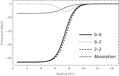
The potentials in Cartesian coordinates are then mapped onto a radial coordinate space, as shown in Fig. 1. This potential can be fitted for the parameters, $V_{0}$, $a_{0}$, and $R_{0}$, using a Newtonian least squares regression, to create an effective Woods-Saxon potential defined as:

$$V_{N}=\frac{V_{0}}{1+\exp(\frac{r-R_{0}}{a_{0}})}.$$ (1)

Here $V_{0}$ is the strength of the potential, $a_{0}$ defines the diffuseness of the potential and $R_{0}$ is the radius of the nucleus defined as $R_{0}=r_{0}(A_{T}^{\frac{1}{3}}+A_{P}^{\frac{1}{3}})$ where $A_{T,P}$ are the atomic numbers for the target and projectile, where for the neutron $A_{P}$ is 1, and $r_{0}$ is a radius parameter.

Figure 1: The nuclear interaction potential between a neutron and the ¹⁸⁸Os target is generated from the Sky3D code with a Woods-Saxon shaped line fitted to the data for ¹⁸⁸Os+n using a Newtonian least-squares regression. The parameterisation data for ¹⁸⁸Os+n is shown in Table 1.

The WS potential is unable to fit the HF potential at small radii because of shell effects in the HF potential. These shell effects are irrelevant in TDCCWP because of the phenomenological absorption potential and the reflective wall at the origin, converting any negative radii into an equivalent positive radius, an equivalent reflection about the origin. This boundary is created by the discrete-variable-representation (DVR) of the kinetic energy [33]. Therefore, the points within 2 fm are omitted, but are shown in Fig. 1 to show the full many-body potential. The fitted parameters used are shown in Table 1. As well as the parameters from the Hartree-Fock model the global optical model parameters are shown, which are the parameters used in many reaction models, such as TALYS, which use an energy dependent potential strength. The maximum and minimum values of the incident energy are selected and shown in Table 1 which are calculated using the Koning-Delaroche parameterisation [17] or the HF model.

Table 1: The fitted Woods-Saxon parameters for the static HF potential of ¹⁸⁸Os+n shown in Fig. 1 along with the set of global optical model parameters. The potential strength is energy dependent, so the maximum and minimum incident energy of the neutron are selected.

Type	$V_{0}$ (MeV)	$a_{0}$ (fm)	$R_{0}$ (fm)
Hartree-Fock	$-42.9311$	$0.6129$	$7.3033$
Koning-Delaroche $E_{i}=10$ keV	$-48.5707$	$0.65$	$7.07$
Koning-Delaroche $E_{i}=500$ keV	$-48.4031$	$0.65$	$7.07$

A comparison of the percentage difference between the capture probabilities calculated with the Koning-Delaroche parameters against the HF parameters is shown in Fig. 2. It can be seen that at the highest energies a difference of 0.02% in transmission coefficients is seen from the HF values. As the thermal energy of the model increases, this percentage difference increases, showing an important relationship between the nuclear potential parameters and the capture probabilities. However, the difference between energies used in the Koning-Delaroche parameterisation results in changes in transmission coefficients of less than 0.001%. This means that using $E_{i}=10-500$ keV does not result in a large difference in transmission coefficients. The HF potential model is used to implement a many-body microscopic potential.

Figure 2: The percentage difference, $100*\frac{T_{KD}-T_{HF}}{T_{HF}}$, of the $l=0$ transmission coefficients calculated with Koning-Delaroche (KD) and HF nuclear potentials, using the deformation parameters from Table 2. The potential parameters are given in Table 1. A difference of 0.02% in capture probabilities is shown for the largest incident energies.

II.3 Initialisation of the wave-packet and system

To initialise the system, the general form of a Gaussian wave-packet is used to model the initial ($t=0$) radial wave-function of the neutron-osmium system as shown:

$$\psi(r)=\mathcal{N}^{-\frac{1}{2}}\exp\bigg(\frac{(r-x_{0})^{2}}{2\sigma_{0}^{2}}\bigg)\exp(-iK_{0}r).$$ (2)

This uses $\mathcal{N}=\langle\psi|\psi\rangle$ as the normalisation of the wave-function, $x_{0}$ as the initial position of the wave-packet, and $K_{0}$ as the wave-number determined by the initial incident energy of the wave-packet. The spatial width of the wave-packet is defined as $\sigma_{0}$, which also defines the energy resolution of the model. In other words, a wider wave-packet will give a narrower momentum-space wave-packet from the inverse relation between spatial width and momentum width. Furthermore, a narrow energy resolution corresponds to a small momentum width and therefore a large width in position, $\sigma_{0}$. The fluctuation of this energy is determined by $\Delta E=\frac{\hbar^{2}}{4\mu\sigma_{0}^{2}}$. Choosing a larger width requires a larger grid size and, therefore, more grid points for accurate resolution. This then increases the computational time of the model. The selected width of 50 fm is chosen to reduce the computational time with the required resolution, and gives an error in energy of 0.004 keV. It can be shown that with a larger width of 80 fm, there is a percentage difference, from the $50$ fm results, of $<1\%$ in transmission coefficients.

Table 2: The initial parameters for the grid size, the wave-packet, and absorptive potential parameters are shown with a description of each parameter used.

Parameter	Value	Description
N	$400$	Number of grid points
$r_{min}$	$0.5$ fm	Minimum radius of the grid
$r_{max}$	$500.5$ fm	Maximum radius of the grid
$\Delta t$	$0.1$ zs	Time step in propagation
$x_{0}$	$150$ fm	Initial position of wave-packet
$\sigma_{0}$	$50$ fm	Initial width of wave-packet
$\beta_{2}$	0.179	188Os quadrupole deformation [42]
$\beta_{4}$	-0.059	188Os hexadecapole deformation [42]
$V_{W0}$	-7 MeV	Absorption potential strength
$a_{W0}$	0.75 fm	Absorption diffuseness
$R_{W0}$	5 fm	Radius where absorption is centered

II.4 Thermalisation of the wave-packet

The wave-packet can be split into $n$ parts, for each of the internal energy levels of the target. Each of these components of the wave-packet corresponds to the interaction of the neutron with the nucleus in the given excited state. The first of these components is the interaction with the ground state, the second is the interaction with the first excited state, and so on. To thermalise the system, Boltzmann factors are used to generate an initial probability for the wave-packet to populate a certain energy while the environment is at a particular temperature. The definition of the general form of the components of the wave-packet is defined below:

$$|\psi\rangle=\sqrt{p_{0}}|\psi_{0}\rangle+\sum_{n=1}^{N}\sqrt{\exp\bigg({-\frac{\epsilon_{n}}{kT}}\bigg)}|\psi_{n}\rangle.$$ (3)

The variable $\epsilon_{n}$ is the energy of the $n^{th}$ excited state, $k$ is the Boltzmann constant, and $T$ is the temperature of the environment. The value of $p_{0}$ is calculated through exploiting the normalisation condition of the wave-packet, $p_{0}=1-\sum_{n=1}^{N}p_{n}$. Applying this general form to the case where there are two channels gives [21]:

$$|\psi\rangle=\sqrt{1-p_{1}}|\psi_{0}\rangle+\sqrt{p_{1}}|\psi_{1}\rangle.$$ (4)

It is defined that $p_{1}=\exp({-\frac{\epsilon_{1}}{kT}})$, which gives the initial probability of the first excited state at some temperature. This use of Boltzmann factors is a good assumption for collision timescales larger than one zeptosecond, since thermal equilibrium will be reached before the reaction takes place [4].

Previous work has used the Maxwell-Boltzmann velocity distribution to apply thermal effects directly in the calculation of reaction rates separately for the decays of individual excited states [26, 11]. This Hauser-Feshbach style calculation is done by running a single-channel calculation of TDCCWP for the ground and excited states separately over a range of incident energies from 10-500 keV. These energies are shifted by $E=E_{0}-\epsilon$, so the effective incident energies for the excited states is shifted by the excited state energy, $\epsilon$, to have effective energies in the range 10-500 keV. Then each of these components of the cross section are independently used to create reaction rates for each internal energy level. These reaction rates are then combined to create the total temperature dependent reaction rate in the Hauser-Feshbach style calculation, as explained in subsection II K.

II.5 Hamiltonian for the coupled channels method

In order to include energy levels of ¹⁸⁸Os in the Hamiltonian, the coupled channels framework is implemented. The Hamiltonian must now be extended to account for the interactions of the neutron with the target relating to the ground and first excited states. The ground state Hamiltonian is described as:

$$\hat{H}_{0}=-\frac{\hbar^{2}}{2\mu}\frac{d^{2}}{dr^{2}}+\frac{\hbar^{2}l(l+1)}{2\mu r^{2}}+V_{N}(r)+iW(r).$$ (5)

The first term here is calculated using the DVR method [33] and the second is the centrifugal potential. The $V_{N}(r)$ defines the nuclear interaction potential of the system, and the $W(r)$ is the absorption potential. The complete coupled channels Hamiltonian can be described by a matrix as shown below:

$$\hat{H}|\psi\rangle=\pmatrix{\hat{\hfil}}{H}_{0}+V_{0-0}&V_{0-2}\\ V_{2-0}&\hat{H}_{0}+V_{2-2}+\epsilon_{2}\pmatrix{|}\psi_{0}\rangle\\ |\psi_{2}\rangle.$$ (6)

Here and for many other even-even nuclei, $0^{+}$ is the ground state and $2^{+}$ is the first excited state, and so referred to as 0 and 2 throughout. These labels specify the state of the ground and first excited states, respectively, for the ¹⁸⁸Os ground-state rotational band. For the odd mass nuclei and odd-odd nuclei, this process is slightly different [35]. The first entry in the Hamiltonian, 0-0, is identical to the case without coupling and corresponds to the ground state, while the final entry, 2-2, is the Hamiltonian of the first excited state, which contains the interaction of the neutron with the first excited state along with the energy shift of this state, $\epsilon_{2}$. Furthermore, the off-diagonal entries, $V_{0-2}$ and $V_{2-0}$, give the components of the Hamiltonian relating to couplings between the ground state and the first excited state. The wave-packet also requires components corresponding to the ground state and first excited state interaction. If there were more than 2 states, this would then be generalised with an $n\times n$ matrix with the number of excited states, $n-1$, as well as a wave-function with $n$ parts [39]. However, 2 states are used here since there is an insignificant difference, $<$ 0.1%, in cross sections between 2 and 3 states, and using 2 states greatly reduces computational time. This could be another area that defines the error of the model; however is generally a smaller contribution than increasing the width parameter to reduce energy width. The calculation of these coupling potentials is now shown in the next section.

Figure 3: All of the different potentials in the model for the ¹⁸⁸Os+n reaction are presented, including the coupling potential. Note the positioning of the absorption potential, which is more central than the coupling potential and well inside the nuclear interaction region. The 0-2 shows the coupling between the ground and first excited state.

II.6 The Coupled Channels Potential

The above effect of couplings on the Hamiltonian, is implemented through a displacement of the nuclear potential for each of the excitations. Moreover, this coupled-channel approach creates a new potential describing the coupling between energy levels of the interacting system. This coupling potential is shown below, where $\hat{r}_{cc}$ is a dynamical operator of the coupling matrix that defines the displacement of the potential due to couplings, where now the

$$V_{cc}=\frac{V_{0}}{1+\exp((r-R_{0}-\hat{r}_{cc})/a_{0})}.$$ (7)

This new form of the potential can then be used in order to define the effects of excitations and de-excitations from one channel to the next. The general form of the total coupling potential is [13]: V_N,nn’=⟨I_n—V_N(r,^r_cc)—I_n’⟩-V_N(r,0)δ_nn’
=∑_α⟨I_n—α⟩⟨α—I_0’⟩V_N(r,r_cc,α)-V_N(r,0)δ_nn’.

In the above $\hat{r}_{cc}|\alpha\rangle=r_{cc,\alpha}|\alpha\rangle$ where the eigenstates $|\alpha\rangle$ are created from the basis spin states $|I_{n}\rangle$, which define the energy levels of ¹⁸⁸Os. The second term, which includes the delta function, is used for the case of the potentials for the ground and first excited states coupling to themselves and avoids the double counting of the original nuclear potential $V_{N}$ from above. These eigenstates are then found by diagonalising the following coupling matrix [13]:

$$\langle I_{n}|\hat{r}_{cc}|I_{n^{\prime}}\rangle=R_{cc}(\beta_{2}F(2,I_{n},I_{n}^{\prime})+\beta_{4}F(4,I_{n},I_{n}^{\prime})).$$ (8)

Here $\beta_{2}$ and $\beta_{4}$ are the quadrupole and hexadecapole deformation parameters that define the shape of the target nucleus. These are shown in Table 2. The $R_{cc}$ is the phenomenological value of the coupling radius defined as $R_{cc}=r_{coup}(A_{T})^{\frac{1}{3}}$ fm where $r_{coup}$ is the coupling radius parameter. The function $F$ here is defined below as the form factor, where the bracketed portion is a 3-j symbol.

F(I,I_n,I_n’)=(2I+1)(2In+1)(2In’+1)4π
×(I)_n I I_n’
0 0 0 ^2. For a system of $n$ energy levels, there will be $n$ different coupling eigenvalues from Eq. (8) that are used with Eq. (7) to calculate the full coupling potentials. The $0^{+}$ and $2^{+}$ states are used here. This coupling channel scheme has commonly been used in static coupled channels frameworks such as CCFULL [13] and FRESCO [34]. In the next section, a description of the dynamical extension of this coupled-channel model is shown, along with the implementation of the absorption potential.

II.7 Selection of deformation parameters

Deformation parameters are in general theoretical parameters to hint at the intrinsic shape of the nucleus. Several different methods to calculate these exist and are shown in Table 3 with the values used in the TDCCWP calculation of the ¹⁸⁸Os+n reaction in bold. The impact of changing deformation values on the calculated transmission coefficients in TDCCWP can be seen in Fig. 4 where the differences in transmission coefficients are much less than 1% for any change in the set of deformation parameters.

Table 3: Deformation from different theoretical calculations namely the Potential Energy Surface (PES) model [42] Folded-Yukawa Finite-Range Droplet Model (FY+FRDM) [25], and the Extended Thomas-Fermi plus Strutinsky Integral (ETFSI) method [1]. The experimental estimate calculated from reduced transition probabilities is $\beta_{2}=0.186$ [42]

Model	$\beta_{2}$	$\beta_{4}$
PES	0.179	-0.059
FY $+$ FRDM	$0.192$	$-0.086$
ETFSI	$0.20$	$-0.08$

Figure 4: The percentage difference of $l=0$ transmission coefficients, $100*\frac{T_{FY/ET}-T_{PES}}{T_{PES}}$, of the FY+FRDM and ETFSI deformation models against the PES deformation model, using the HF nuclear potential. The largest percentage difference is  0.2%, which is insignificant.

II.8 The modified Chebyshev method for absorptive dynamics

To understand the probability of a neutron being captured by the nucleus, a phenomenological absorption potential is used. This Woods-Saxon-shaped potential, as defined by Eq. (1), acts to extract normalisation from the incident wave-packet. Some care is needed for the placement of this potential, since the channel couplings need to take effect inside the nucleus before the absorption potential takes away any normalisation from the wave-packet [14]. The positions of these potentials can be seen in Figure 3. A potential too close to the edge of the nuclear radius would not allow any effects from the couplings, whereas a potential too close to the center of the nucleus will not maximally absorb normalisation. This location, described by the parameters in Table 2, still gives maximum absorption at $R_{W0}=5$ fm, but still allows for the couplings to take place. Similarly, the absorption strength of $V_{W0}=-7$ MeV is sufficiently large to have $<0.1\%$ change in cross section if a larger $V_{W0}=-50$ MeV absorption strength was chosen, showing the independence of the cross section on these absorption parameters.

With the inclusion of this absorption potential, the modified Chebyshev propagator is used in the TDCCWP method. The Chebyshev propagator rewrites the exponential time evolution operator as a set of Chebyshev polynomials [7]. In general, using an absorption potential in the Hamiltonian would make the Hamiltonian complex. To deal with this, an operator is used to extract the imaginary part while still using the real part of the Hamiltonian. This method applies a recurrence relation where the absorption potential acts as the wave-packet propagates through time using Chebyshev polynomials [22]. The complete method can be found in [22] and [10]. This method gives the base of the calculation and propagation, and now the intrinsic physics of the excited states are explored using the kinematically closed states first.

II.9 Kinematically Closed States

The movement of the wave-packet along the radial grid is defined by the wave-number of each component that corresponds to an energy level of the ¹⁸⁸Os target. The wave-number of each component of the wave-packet defines the movement of the wave-packet along the radial grid, where the wave-number is given by:

$$K_{n}=\sqrt{\frac{2\mu(E_{0}-\epsilon_{n})}{\hbar^{2}}-\frac{1}{2\sigma_{0}^{2}}}.$$ (9)

From this, $\epsilon_{n}$ is defined as the excited state energy from the ground state. When the excited state energy is greater than the incident energy, $E_{0}$, computing this value requires a negative square root due to a negative value for the energy. To avoid this, it can be noticed that if the incident energy of the wave-packet is below the first excited state, the incident energy can only virtually excite the target nucleus. More specifically, any probability in this excited state is ”stuck” inside the nucleus and does not move along the grid at all. This means that a wave number of $K_{n}=0$ fm^-1 can be used to keep this component of the wave-packet stationary. Therefore, these stationary states correlate to the kinematically closed states in the system.

II.10 Transmission coefficients and the neutron capture cross section

The TDCCWP implementation ends once the wave packet has fully interacted. This is defined when the expectation value of the position of the reflected wave-packet reaches the initial position of the incoming wave-packet. The transmission coefficients are found directly from the reflection coefficients, $\mathcal{R}$, using the relation $\mathcal{T}=1-\mathcal{R}$. In the case with multiple energy levels, both components of the wave-function are summed since both components of the wave-packet lose normalisation from the absorption. Furthermore, the calculation of the cross-section is:

$$\sigma(E_{0},T)=\frac{\pi\hbar^{2}}{2\mu E_{0}}\sum_{l=0}(2l+1)\mathcal{T}(E_{0},l,T).$$ (10)

It can be seen that the transmission coefficients are dependent on incident energy, $E_{0}$, as well as the temperature, $T$, of the environment. The sum over angular momentum in Eq.(10) at low incident energies can typically be omitted due to high centrifugal barriers for non-zero partial waves. The sum over angular momentum reflects more of the wave-packet since the incident energies in neutron capture reactions are generally small, $<$1 MeV. The next step is to understand how these capture cross sections can be used for calculating reaction rates.

II.11 Calculating reaction rates

The reaction rate is defined as the number of reactions that happen per unit time per unit volume. In typical calculations, thermal effects are applied as the reaction rates are calculated using the Maxwell-Boltzmann speed distribution and Boltzmann factors to give probability weightings for thermal effects at each incident energy. However, in this TDCCWP model, the thermal dependence in the reaction rates will be included at the initialisation of the wave-packet. The reaction rate in terms of the new thermal dependence of the cross section is calculated as follows [23, 31]:

$$\langle\sigma v\rangle=\sqrt{\frac{8}{\pi\mu}}\bigg(\frac{1}{kT}\bigg)^{\frac{3}{2}}\frac{\int_{E_{i}}^{E_{f}}{\sigma(E_{0},T)\cdot E_{0}\cdot P(E_{0},T)}dE_{0}}{\int_{E_{i}}^{E_{f}}{E_{0}\cdot P(E_{0},T)}dE_{0}}.$$ (11)

A simple substitution with velocities results in an integral over incident energies; in this calculation, a range of $E_{i}=10$ keV to $E_{f}=500$ keV is used. This also defines $P(E_{0},T)$ as the Maxwell-Boltzmann distribution of neutron incident energies. This substitution gives rise to the pre-factor shown above [23]. It is important to note that the original form of this equation [31] takes the integral from $[0,\infty)$. This would be unphysical here, so to restrict the calculation to a finite range of incident energies, a normalisation factor is included as the denominator in Eq. (13). The cross-section is given by Eq. (12). Previous studies of stellar reaction rates [30] were carried out taking the sum of integrals using Boltzmann factors $p_{n}$:

$$\langle\sigma v\rangle=\sum_{n}p_{n}(\epsilon_{n})\langle\sigma v\rangle_{n}$$ (12)

$$=\sqrt{\frac{8}{\pi\mu}}\bigg(\frac{1}{kT}\bigg)^{\frac{3}{2}}\sum_{n}p_{n}(\epsilon_{n})\frac{\int_{E_{i}}^{E_{f}}{\sigma_{n}(E_{n})\cdot E_{n}\cdot P(E_{n},T)dE_{n}}}{\int_{E_{i}}^{E_{f}}{E_{n}\cdot P(E_{n},T)dE_{n}}}.$$

In this equation each $\langle\sigma v\rangle_{n}$ gives an independent calculation of the reaction rate, where $n$ corresponds to each internal energy level of the target nucleus [30]. Each sum also involves a shift in incident energies which transforms the integral to adjust for the excitation energy of the excited states of the target, $E_{n}=E_{0}-\epsilon_{n}$, where $E_{0}$ is the incident energy of the neutron. As well as this Boltzmann factors $p_{n}$ as described in subsection II D are used account for the probability each excited state has to be populated at a certain thermal energy. This approach neglects the dynamical coupling between the target’s internal thermally populated states during the neutron capture process. However, in TDCCWP the thermal dependence is included from the start of the reaction at the level of the initial wave-function in Eq. (4), which has not been explored in neutron capture cross-sections. In the next section, the results of this temperature dependence are shown against previously used models as well as against the same model, one with a temperature dependence and one without.

III Results

III.1 A comparison with CCDM

A comparison between TDCCWP and the quantum dynamical CCDM method is useful. CCDM has already been validated to match static CCFULL calculations [21, 40], so validate the TDCCWP method simultaneously. CCDM also uses a density matrix formalism to explore coherence effects dynamically, so here compares a calculation with and without the inclusion of coherence effects. This has been used to implement thermal effects on heavy-ion fusion reactions to generate thermally dependent cross sections [20, 21]. The comparison in Fig. 5 shows the difference between mixed and entangled initial states as well as the thermal dependence of neutron capture cross sections.

Figure 5: Transmission coefficients from TDCCWP calculations are compared to those from the CCDM model for the $l=0$ partial wave for the ¹⁸⁸Os+n reaction. Two thermal energies are displayed, these being 0 and 500 keV in thermal energy (kT). The shaded region around the 500 keV TDCCWP results shows the error in the TDCCWP calculation found by finding the percentage change from a wider wave-packet calculation.

Irrespective of the neutron incident energy, the static coupling between the two channels creates two decoupled pathways for the neutron-osmium interaction [21]. These pathways are the eigenstates of the coupling potential matrix, which have separate statistical weights that depend on temperature. As temperature increases, the population of the pathway with the more attractive nuclear interaction increases, while the population of the pathway with the less attractive nuclear interaction decreases [21]. Each of these pathways are a coherent linear superposition of the ¹⁸⁸Os target’s states. Furthermore, each pathway contains the contribution of the target’s ground state, irrespective of the incident energy of the neutron. Therefore, in the case where there is an increase in temperature the neutron’s speed increases in the absorption region. This increase in speed results in a higher probability for the neutron to escape its capture, and therefore a decrease in the capture probability as observed in Fig. 5.

The difference in transmission is obvious between both a density matrix and wave-packet-based formalism, particularly for small incident energies where coherence effects may play a larger role. It can be seen that when generating a transmission coefficient, there is a difference in the calculation below and above the energy of the first excited state (155 keV). A decrease in the transmission can also be seen in the lower energies, reflecting this change. At higher energies, the two converge, reflecting what would be expected for kinematically closed and open channels. In other words, these components can now fully react with the nucleus and are absorbed, as opposed to the ¹⁸⁸Os target being virtually excited when the incident energies are in the kinematically closed region. Despite this, the two quantum dynamical models provide similar transmission coefficients, particularly for the temperature-independent calculation, $kT=0$ keV. However, the TDCCWP method is computationally more efficient.

III.2 A comparison with a Hauser-Feschbach style calculation

Figure 6: Temperature-dependent capture cross sections for a $l=0$ neutron on the ¹⁸⁸Os target as a function of neutron energy using a Hauser-Feshbach and TDCCWP style calculation. A thermal energy of 250 keV is used in both implementations of thermal effects.

To compare with the already existing treatment of thermal effects [26], a Hauser-Feschbach style implementation of thermal effects on cross sections is applied to the TDCCWP method. This is done by using a temperature-independent TDCCWP calculation for the neutron capture cross section in a specific excited state of ¹⁸⁸O, and then applying Boltzmann factors in the same way as in Eq. (12) for reaction rates. This final state implementation, at the cross-section level, neglects the dynamical coupling among ¹⁸⁸O excitations, and is compared to the initial state implementation, at the wave-packet level, present in TDCCWP.

This comparison is shown in Fig. 6 where a reduction in cross section is present when thermal effects are included at the wave-packet level, while an enhancement of cross sections are present when thermal effects are treated at the cross-sectional level. This hints at the interactions between the ground and excited states having a larger involvement in neutron capture reactions, to reduce this enhancement. An increase in cross sections in the Hauser-Feshbach style calculation is also present for large incident energies, while in the TDCCWP model, there is an agreement between the temperature-independent calculation and the temperature-dependent one. The TDCCWP result also displays the inclusion of the kinematically closed state for incident energies up to the first excited state, 155 keV. In the Hauser-Feshbach style calculation, there is more agreement between the temperature-independent calculation for these smaller incident energies.

III.3 Cross Sections

Figure 7: Temperature-dependent capture cross sections for a l=0 neutron on the ¹⁸⁸Os target as a function of the neutron incident energy in the range 140-500 keV. The shaded regions highlight errors associated with the energy variance of the neutron energy (i.e., the differences in the TDCCWP calculations using a spatial width of the initial wave-packet of 50 and 80 fm). The change from the kinematically closed energy region to the open one happens at the ¹⁸⁸Os first excited state energy (155 keV).

To explore more of this difference across the two incident energy regions, the neutron capture cross sections can also be calculated. Fig. 7 shows a kink in the cross-section data where the model transitions from the kinematically closed region, below 155 keV, where there are only virtual excitations to the first excited state, to the region above this where excitations to the first excited state can occur. For higher incident energies, the higher thermal energy and low thermal energy cases both begin to converge to similar values. The resonance region for this reaction is below this first excited state and can be seen in Fig. 8, again showing the discrepancy in capture cross sections when thermal effects are included. The thermal energy of 250 keV (5.8 GK) is chosen to show the large discrepancy when thermal effects are included at the temperature scale of the rapid neutron capture process. These differences persist but are smaller for the temperatures corresponding to the slow neutron capture process (0.1-1 GK), which is the process that dominates for this isotope [3].

Figure 8: The same as in Fig. 7, however, the range of incident energies is 10-140 keV.

This comparison can be continued for the higher angular momentum contributions as shown in Fig. 9. It can be seen that the contributions at the lower incident energies are much less for the higher angular momenta, giving the convergence of the system. For many of the energies below the first excited state and in the region of importance for resonances, the $l=2$ angular momentum contribution is less than a tenth of the total capture cross section. This can be continued and shown to converge as the angular momentum increases. However, for many of these low incident energies, the $l=2$ component is the highest that needs to be included to show convergence of the cross-section.

The next step is to explore how a calculation of reaction rates is changed when cross sections with temperature included at the initialisation of the wave-packet are used used instead of the general inclusion of thermal effects after cross sections have been calculated.

Figure 9: A comparison between the capture cross sections in the $l=0$ and $l=2$ angular momentum states. With each higher angular momentum, the centrifugal barrier reflects more of the incident wave-packet, resulting in the ability to truncate the higher angular momentum components of the cross-section. This truncation will occur at the angular momentum, determined by when the component of cross-section is $<1\%$ of the total cross-section. This cut-off depends on the incident energy being large enough to overcome the height of the centrifugal barrier at a certain angular momentum.

III.4 Reaction Rates

The reaction rate is specifically applicable to astrophysical data analysis, where accurate reaction rates give a sense of how experimental cross sections can be mapped onto astrophysical data. In the neutron capture reaction, this means accurate reaction rates describe how likely these reactions are to take place at different temperatures, ultimately highlighting the importance of the temperature of the environment on the neutron capture reaction as a whole.

In Figure 10, two distinct regions of the temperature range are present. The first region shows an agreement between the two TDCCWP with and without temperature dependencies for thermal energies below $100$ keV. The second is where the TDCCWP calculation with thermal effects shows a decrease in reaction rate compared to the temperature-independent case. For low thermal energies, specifically those present in the slow-neutron capture regime, s-process, $kT<30$ keV, this agreement of reaction rates is present. This may explain why the slow neutron capture regime is dominant for this isotope. Since the reaction rate only decreases for temperatures much larger than temperatures generally present in the s-process, $kT>100$ keV, this could hint at why the s-process dominates the reaction mechanism in the osmium isotopes [15]. This $10\%$ reduction in reaction rates for $kT=250$ keV could highlight the reason why the synthesis of the ¹⁸⁸Os is not generally found in r-process environments, but are found in s-process environments at much lower temperatures. The first step in this process would be to look at isotopes that are dominated by the r-process to show the validity of this statement. Neutron-rich isotopes of californium exhibit this agreement in reaction rates for higher thermal energies [12].

In contrast to TDCCWP, the Hauser-Feshbach style calculation displays a $10\%$ increase in reaction rate in Fig. 10. This discrepancy hints at the value of including an initial thermalisation of the wave-packet to allow for the interaction of the target’s ground and excited states due to nuclear coupling as shown by TDCCWP.

Figure 10: Reaction rates with different types of cross sections from TDCCWP and Hauser-Feshbach style calculations are shown with varied temperature, referred to as thermal energy here, from it being in the form of $kT$. For TDCCWP there is an agreement in reaction rate for the thermal energies below the first excited state and a decrease in reaction rate for thermal energies far above this. For $kT=250$ keV, there is a 10$\%$ reduction in reaction rate, which is directly related to the reduction in capture probability with an increase in temperature. The opposite is seen for the Hauser-Feshbach style calculations, where an increase in 10$\%$ is seen for the same thermal energy. An inset graph shows the fraction between cross sections, $\frac{\sigma(E,T)}{\sigma(E)}$, where the gray line would show perfect agreement.

IV Conclusion

This paper presents the TDCCWP model to display the importance of thermal effects in reaction cross-sections in the ¹⁸⁸Os+n reaction as a test case. Transmission coefficients were generated to calculate cross-sections and reaction rates, including thermal effects at the initialisation step. Firstly, the comparison between the TDCCWP and CCDM methods was shown to agree for high incident energies and show a decrease in capture probability in TDCCWP for low incident energies when thermal effects are included. Subsequently, temperature-dependent cross sections were shown to exhibit a decrease in cross section for an increase in temperature, contrary to applying thermal effects to cross sections as commonly done in the literature. This change was highlighted by a decrease in reaction rates at high thermal energies, up to a $10\%$ reduction at $kT=250$ keV, which may hint at an importance in including thermal effects in this way for r-process reactions. This change in reaction rates for the dominant s-process at $kT=30$ keV is much less and shows an increase of $2\%$.

Further work will address thermal effects in neutron capture reactions involving osmium and rhenium isotopes. This would give a better understanding of the contribution of thermal effects in the neutron capture cross sections throughout the Re-Os chain. In addition, this could elaborate on the temperature-dependent contribution of the abundance of ¹⁸⁷Os from neutron capture reactions. This would work in contrast to the abundance of ¹⁸⁷Os from the $\beta_{-}$ decay from ¹⁸⁷Re, ultimately giving another estimate for stellar enhancement factors and for the age of the universe using the Re-Os clock. Subsequently, other isotopes could be explored, such as ⁹⁹Zr, which is specifically applicable as an unstable byproduct in nuclear reactors. Finally, californium, relevant to the r-process, can be studied to highlight the change in cross sections and reaction rates at high temperatures present in these reactions, where the results from when the thermal effects are included differ the most. These extensions are all valuable for both low-energy neutron physics and for exploring the resonance regions of these isotopes [38].

V Acknowledgments

This was supported by the UK Science and Technology Facilities Council (STFC) under Grants No. ST/Y509619/1, ST/V001108/1 and ST/Y000358/1.

VI Data Availability

The data that support the findings of this article are not publicly available. The data is available from the authors upon reasonable request.

References

- [1] (1995) Nuclear mass formula via an approximation to the hartree—fock method. Atomic Data and Nuclear Data Tables 61 (1), pp. 127–176. Cited by: Table 3.
- [2] (2023) Origin of the elements. The Astronomy and Astrophysics Review 31 (1), pp. 1. Cited by: §I.
- [3] (2011) Tungsten isotopic compositions in stardust sic grains from the murchison meteorite: constraints on the s-process in the Hf–Ta–W–Re–Os region. The Astrophysical Journal 744 (1), pp. 49. Cited by: §III.3.
- [4] (1984) Approach to chemical equilibrium in thermal models. Physical Review C 29 (3), pp. 967. Cited by: §II.4.
- [5] (2015) Quantifying low-energy fusion dynamics of weakly bound nuclei from a time-dependent quantum perspective. Physical Review C 92 (4), pp. 044610. Cited by: §I.
- [6] (2013) FRESCO, a simplified code for cost analysis of fusion power plants. Fusion Engineering and Design 88 (12), pp. 3141–3151. Cited by: §I.
- [7] (1999) The chebyshev propagator for quantum systems. Computer Physics Communications 119 (1), pp. 19–31. Cited by: §II.1, §II.8.
- [8] (2025) Quantum dynamical microscopic approach to stellar carbon burning. Physics Letters B 870, pp. 139881. External Links: ISSN 0370-2693, Document, Link Cited by: §I.
- [9] (2024) Cluster effects on low-energy carbon burning. Physics Letters B 849, pp. 138476. Cited by: §I.
- [10] (2018) Characterizing the astrophysical S factor for 12C+ 12C fusion with wave-packet dynamics. Physical Review C 97 (5), pp. 055802. Cited by: §I, §II.1, §II.8.
- [11] (2010) Neutron physics of the Re/Os clock. iii. resonance analyses and stellar (n, ) cross sections of 186,187,188Os. Physical Review C 82 (1), pp. 015804. Cited by: §I, §II.4.
- [12] (1977) A californium-252 fission spectrum irradiation facility for neutron reaction rate measurements. Nuclear Technology 32 (3), pp. 315–319. Cited by: §III.4.
- [13] (1999) A program for coupled-channel calculations with all order couplings for heavy-ion fusion reactions. Computer Physics Communications 123 (1-3), pp. 143–152. Cited by: §I, §II.6, §II.6, §II.6.
- [14] (1984) The neutron optical potential. Reports on Progress in Physics 47 (6), pp. 613. Cited by: §II.8.
- [15] (2007) S-process implications from osmium isotope anomalies in chondrites. The Astrophysical Journal 664 (1), pp. L59. Cited by: §III.4.
- [16] (2000) Bound state beta-decay and its astrophysical relevance. AIP Conference Proceedings 529 (1), pp. 322. Cited by: §I.
- [17] (2005) TALYS: comprehensive nuclear reaction modeling. AIP Conference Proceedings 769 (1), pp. 1154. Cited by: §I, §II.2.
- [18] (2001) Nuclear reactions and stellar processes. Reports on Progress in Physics 64 (12), pp. 1657. Cited by: §I.
- [19] (2024) Quantum mechanical treatment of nuclear friction in coupled-channels heavy-ion fusion. Physics Letters B 854, pp. 138755. Cited by: §I.
- [20] (2022) Coherence dynamics in low-energy nuclear fusion. Physics Letters B 827, pp. 136970. Cited by: §I, §III.1.
- [21] (2023) Thermal and atomic effects on coupled-channels heavy-ion fusion. Physical Review C 107 (5), pp. 054609. Cited by: §I, §II.4, §III.1, §III.1.
- [22] (1995) Bound states and resonances of the hydroperoxyl radical HO2: an accurate quantum mechanical calculation using filter diagonalization. The Journal of Chemical Physics 103 (23), pp. 10074–10084. Cited by: §II.1, §II.8.
- [23] (2019) Nuclear and particle physics: an introduction. John Wiley & Sons. Cited by: §II.11, §II.11.
- [24] (2014) The TDHF code Sky3D. Computer Physics Communications 185 (7), pp. 2195–2216. Cited by: §II.2.
- [25] (1995) At. data nucl. data tables. At. Data Nucl. Data Tables 59, pp. 185. Cited by: Table 3.
- [26] (2010) Neutron physics of the Re/Os clock. i. measurement of the (n, ) cross sections of 186Os, 187Os, 188Os at the CERN n_TOF facility. Physical Review C 82 (1), pp. 015802. Cited by: §I, §II.4, §III.2.
- [27] (2005) Reaction rate theory: what it was, where is it today, and where is it going?. Chaos: An Interdisciplinary Journal of Nonlinear Science 15 (2), pp. 026116. Cited by: §I.
- [28] (2012) Sensitivity of astrophysical reaction rates to nuclear uncertainties. The Astrophysical Journal Supplement Series 201 (2), pp. 26. Cited by: §I.
- [29] (2000) Astrophysical reaction rates from statistical model calculations. Atomic Data and Nuclear Data Tables 75 (1), pp. 1–351. External Links: ISSN 0092-640X, Document, Link Cited by: §I.
- [30] (2022) Stellar neutron capture reactions at low and high temperature. The European Physical Journal A 58 (11), pp. 214. Cited by: §II.11, §II.11.
- [31] (1988) Cauldrons in the cosmos: nuclear astrophysics. University of Chicago press. Cited by: §II.11, §II.11.
- [32] (2007) Neutron capture cross sections of 186Os,187Os and 189Os for the Re-Os chronology. Physical Review C 76 (2), pp. 022802. Cited by: §I.
- [33] (1992) Quantum mechanical reaction probabilities via a discrete variable representation-absorbing boundary condition green’s function. The Journal of Chemical Physics 97 (4), pp. 2499–2514. Cited by: §II.2, §II.5.
- [34] (1988) Coupled reaction channels calculations in nuclear physics. Computer Physics Reports 7 (4), pp. 167–212. Cited by: §II.6.
- [35] (2014) Coupled-channel models of direct-semidirect capture via giant-dipole resonances. Nuclear Data Sheets 118, pp. 292–294. Cited by: §II.5.
- [36] (2024) Laser-assisted deuterium-tritium fusion: a quantum dynamical model. Physical Review C 110, pp. 034614. Cited by: §I.
- [37] (2025) Enhancing the creation of elements in laser-assisted heavy-ion fusion reactions. Physical Review C 112, pp. 014604. Cited by: §I.
- [38] (1969) Slow neutron total cross-sections and resonance levels of osmium-187, 188 and 189. The Ukranian Journal of Physics 14 (12), pp. 1971. Cited by: §IV.
- [39] (2019) Describing heavy-ion fusion with quantum coupled-channels wave-packet dynamics. Physical Review C 100 (3), pp. 034606. Cited by: §I, §II.5.
- [40] (2021) Calculating the S-matrix of low-energy heavy-ion collisions using quantum coupled-channels wave-packet dynamics. Physical Review C 104 (6), pp. 064601. Cited by: §I, §III.1.
- [41] (2021) Quantum dynamics of heavy-ion collisions at coulomb energies using the time-dependent coupled-channel wave-packet method. Ph.D. Thesis, University of Surrey. External Links: Document Cited by: §I.
- [42] (2015) Nuclear stiffness evolutions against axial and non-axial quadrupole deformations in even-a osmium isotopes. Progress of Theoretical and Experimental Physics 2015 (7), pp. 073D03. Cited by: Table 2, Table 2, Table 3.
- [43] (2025) Quantum physics of stars. Reviews of Modern Physics 97 (2), pp. 025003. Cited by: §I.
- [44] (1987) Maxwellian-averaged neutron capture cross sections for 99Tc and 95-98Mo. Astrophysical Journal 313, pp. 808. Cited by: §I.