A Parameter-free Decentralized Algorithm for Composite Convex Optimization Thanks: Chen and Scutari are with the School of Industrial Engineering, Purdue University; emails:<chen4373,gscutari>@purdue.edu. Kuruzov and Gasnikov are with the Innopolis University; emails: kuruzov.ia@phystech.edu, gasnikov@yandex.ru.

Abstract

The paper studies decentralized optimization over networks, where agents minimize a composite objective consisting of the sum of smooth convex functions–the agents’ losses–and an additional nonsmooth convex extended value function. We propose a decentralized algorithm wherein agents adaptively adjust their stepsize using local backtracking procedures that require no global (network) information or extensive inter-agent communications. Our adaptive decentralized method enjoys robust convergence guarantees, outperforming existing decentralized methods, which are not adaptive. Our design is centered on a three-operator splitting, applied to a reformulation of the optimization problem. This reformulation utilizes a proposed BCV metric, which facilitates decentralized implementation and local stepsize adjustments while guarantying convergence.

I Introduction

Consider the following decentralized optimization

$$\min_{x\in\mathbb{R}^{d}} u(x):=f(x)+r(x),$$ (P)

$$f(x):=\frac{1}{m}\sum_{i=1}^{m}f_{i}(x),\vskip-5.69046pt$$ (1)

where $f_{i}:\mathbb{R}^{d}\to\mathbb{R}$ is the cost function of agent $i\in[m]:=\{1,\ldots,m\}$, assumed to be convex, locally smooth, and known only to the agent; $r:\mathbb{R}^{d}\to\mathbb{R}\cup\{-\infty,+\infty\}$ is a convex, nonsmooth function, known to all agents, which can be used to enforce shared constraints or specific structures on the solution (e.g., sparsity or low-rank). Agents are embedded in a mesh communication network, modeled as a fixed, undirected and connected graph $\mathcal{G}$ with no servers.

Problem (P) arises from several applications of interest, including signal processing, machine learning, multiagent systems, and communications. The literature abounds with decentralized solution methods for (P) (when $f_{i}$’s are globally smooth); we refer to the recent tutorial (and reference therein) [1] and book [2] for a detailed review. These methods commonly rely on conservative stepsize bounds for convergence, dependent on parameters such as the Lipschitz constants of the agents’ gradients, the spectral gap of the graph adjacency matrix, or other topological properties. However, this crucial information is not locally available to the agents. Consequently, stepsize values are often set through manual tuning, leading to performance that is unpredictable, problem-dependent, and not reproducible. Furthermore, these methods fails when agents’ losses are only locally smooth–refer to Sec.I-B for more information. This paper brings adaptivity to the decentralized setting (P).

I-A Main contributions

1. Algorithm design: We introduce an adaptive decentralized algorithm tailored to the composite structure of Problem (P). To deal with the nonsmooth term, our design leverages a three-operator splitting decomposition. This is applied to a reformulation of (P) based on the BCV technique [3, 4] (named after Bertsekas, O’Connor, and Vandenberghe). A suitable metric is chosen in the BCV transformation, to facilitate a fully decentralized implementation of the splitting-based algorithm that uses only neighboring communications while enabling adaptive updates of the agents’ stepsize through local backtracking procedures. Remarkably, our algorithm does not require agents to know any global optimization or network parameters.

2. Convergence guarantees: We rigorously prove convergence of the proposed method, demonstrating a sublinear $\mathcal{O}(1/k)$ rate for a suitably defined optimality gap, where $k$ denotes the iteration count. Preliminary numerical results highlight that our adaptive algorithm significantly outperforms existing decentralized algorithms applicable to (P), all of which rely on nonadaptive stepsize choices.

I-B Related works

1. Adaptive centralized methods: In recent years, there has been an increasing interest in developing adaptive (a.k.a. parameter-free) optimization algorithms for centralized and federated settings. These methods include established techniques such as line-search approaches [3], Polyak’s stepsize [5], Barzilai-Borwein’s stepsize [6], as well as more recent advancements that estimate the local curvature of the cost function [7, 8, 9]. Additionally, other adaptive gradient methods tailored specifically to machine learning challenges include AdaGrad [10], Adam [11], AMSGrad [12], NSGD-M [13], and their variants [14, 15]. Some of these algorithms have been adapted for federated architectures (server-client systems) [16, 17, 18]. However, these methods are not suitable for mesh networks because they rely on a central server to aggregate local model updates and tune the common stepsize–a process impractical in decentralized mesh setups. Among these methods, only [9, 5, 8, 10] can deal with nonsmooth convex terms, as in Problem (P).

2. Adaptive decentralized methods: The landscape of parameter-free decentralized methods is limited, with notable proposals including [19, 20, 21, 22, 9, 23]. Specifically, [19, 20, 21] study stepsize adaptivity for stochastic (non)convex/ online and smooth optimization, typically using gradient normalization from past iterates. Except for [21], these methods assume globally Lipschitz continuous losses, enabling convergence with standard stepsizes of the order $\mathcal{O}(1/\sqrt{k})$ (here, $k$ is the iteration index). Additionally, [19, 20] require prior knowledge of certain problem-dependent parameters. The work [23] introduces a Port-Hamiltonian System framework for smooth, strongly convex, and unconstrained problems. While parameter-free convergence holds in the centralized setting, convergence (global asymptotic stability) in decentralized settings is ensured only under specific graph structures or graph-dependent stepsize constraints, which rely on global network information. No explicit convergence rate expression is provided. Recently, [22] proposed a parameter-free decentralized method for smooth, strongly convex instances of (P), establishing linear convergence and demonstrating superior theoretical and practical performance compared to non-adaptive decentralized algorithms.

None of the decentralized methods described above handle composite optimization problems as (P), nor do they account for locally smooth losses. While proximal adaptive methods for composite optimization have been studied in centralized settings [24, 25], their adaptations to decentralized problems exhibit significant practical limitations. Specifically, the decentralization of [24] requires at every line-search step (i) transmission of ambient-sized vectors–causing prohibitive communication costs–and (ii) computation of the smallest agents’ line-search stepsize across the entire network. The method from [25], while avoiding line-search procedures, still necessitates computing and propagating global scalars at each iteration for stepsize and relies on knowledge of a global network quantity unavailable locally. Resorting to conservative local overestimates of this parameter reduces adaptivity, slows convergence, and makes the algorithm sensitive to critical tuning parameters. These practical drawbacks are confirmed by numerical results in Sec. IV.

In summary, existing adaptive decentralized methods cannot solve composite optimization problems (P) using only neighbor communications. To the best of our knowledge, the parameter-free decentralized algorithm presented here is the first to address this critical challenge.

II Algorithm Design

We study (P) under the following assumptions.

Assumption 1.

(i) Each $f_{i}:\mathbb{R}^{d}\rightarrow\mathbb{R}$ is convex on $\mathbb{R}^{d}$ and locally smooth; (ii) $r:\mathbb{R}^{d}\rightarrow\mathbb{R}\cup\{-\infty,\infty\}$ is convex, proper and lower-semicontinuous; and (iii) $u:\mathbb{R}^{d}\rightarrow\mathbb{R}$ is lower bounded.

Assumption 2.

The network is modeled as an undirected, connected graph $\mathcal{G}=(\mathcal{V},\mathcal{E})$, where $\mathcal{V}=[m]$ and $(i,j)\in\mathcal{E}$ if and only if there is a link between agent $i$ and $j$.

Assumption 3 (Gossip matrices).

Let $W_{\mathcal{G}}$ denote the set of symmetric, doubly stochastic, gossip matrices $\widetilde{W}:=(\widetilde{w}_{ij})_{i,j=1}^{m}$ that are compliant with $\mathcal{G}$, i.e., $\widetilde{w}_{ii}>0$, for all $i\in[m]$; $\widetilde{w}_{ij}>0$ for all $(i,j)\in\mathcal{E}$; and $\widetilde{w}_{ij}=0$ otherwise.

Assumption 1 requires only local smoothness of the losses, which significantly enlarges the class of covered functions and applications. Examples include covariance estimation problems and Poisson inverse problems [26, 27, 28] arising from image processing. Assumption 3 is standard in the literature of gossip-based algorithms–see, e.g., [1, 2].

II-A A three-operator splitting-based algorithm

The starting point of our new algorithm design is the following reformulation of (P) leveraging the BCV technique: introducing local copies $x_{i}\in\mathbb{R}^{d}$ of $x$ and slack variables $\tilde{x}_{i}\in\mathbb{R}^{d}$, along with the row-wise stack matrices $\mathbf{X}:=[x_{1},\ldots,x_{m}]^{\top}$ and $\tilde{\mathbf{X}}:=[\tilde{x}_{1},\ldots,\tilde{x}_{m}]^{\top}$, the following optimization problem

$$\min_{\mathbf{X},\widetilde{\mathbf{X}}\in\mathbb{R}^{m\times d}}\underbrace{F(\mathbf{X})}_{:=\widetilde{F}(\mathbf{X},\widetilde{\mathbf{X}})}+\underbrace{R(\mathbf{X})+\delta_{\{\mathbf{0}\}}(\widetilde{\mathbf{X}})}_{:=\widetilde{R}(\mathbf{X},\widetilde{\mathbf{X}})}+\underbrace{\delta_{\{\mathbf{0}\}}(\text{\L}\mathbf{X}+M\widetilde{\mathbf{X}})}_{:=\widetilde{G}(\mathbf{X},\widetilde{\mathbf{X}})}.$$ (P^′)

is equivalent to the original Problem (P). In (P′), we defined

$$F(\mathbf{X}):=\sum_{i=1}^{m}f_{i}(x_{i}),\quad R(\mathbf{X}):=\sum_{i=1}^{m}r(x_{i});$$

$\delta_{\{\mathbf{0}\}}:\mathbb{R}^{m\times d}\to\mathbb{R}\cup\{\infty\}$ is the indicator function of $\{\mathbf{0}\}$; $\text{\L}\in\mathbb{S}^{m}$ satisfies $\texttt{null}(\text{\L})=\texttt{span}(\mathbf{1}_{m})$, and $M\in\mathbb{S}^{m}_{++}$ is the BCV metric. The matrix Ł enforces consensus among the agents’ variables $x_{i}$’s via $\text{\L}\mathbf{X}=\mathbf{0}$. The choice of $M$ will be shown to be crucial to enable a fully decentralized implementation of the proposed algorithm as well as adaptive local stepsize selection. This justifies the presence of $\widetilde{G}$ in (P′), which is unconvential in the classical decentralized optimization literature. Here, $\mathbb{S}^{m}$ (resp. $\mathbb{S}^{m}_{++}$) denotes the set of $m\times m$ real symmetric (resp. positive definite) matrices.

Problem (P′) is equivalent to solving the monotone inclusion based on the following three-operator splitting [29]:

$$\text{find }\mathbf{T}:=\begin{bmatrix}\mathbf{X}\\ \widetilde{\mathbf{X}}\end{bmatrix}\in\mathbb{R}^{2m\times d}\text{ s.t. }0\in({\mathbb{A}}+{\mathbb{B}}+{\mathbb{C}})\mathbf{T},$$ (2)

where ${\mathbb{A}}:=\partial\widetilde{G}$, ${\mathbb{B}}:=\partial\widetilde{R}$ and ${\mathbb{C}}:=\nabla\widetilde{F}$. Invoking the Davis-Yin three-operator splitting [30], (2) is equivalent to

$$\text{find }\mathbf{T},\mathbf{Z}\in\mathbb{R}^{2m\times d}\,\text{ s.t. }\,\mathbb{D}_{\alpha}\mathbf{Z}=\mathbf{Z}\,\text{ and }\,\mathbf{T}=\mathbb{J}_{\alpha\mathbb{B}}\mathbf{Z},$$ (3)

where

$$\mathbb{D}_{\alpha}:=\mathbb{I}-\mathbb{J}_{\alpha\mathbb{B}}+\mathbb{J}_{\alpha\mathbb{A}}\circ(2\mathbb{J}_{\alpha\mathbb{B}}-\mathbb{I}-\alpha\mathbb{C}\circ\mathbb{J}_{\alpha\mathbb{B}}),$$ (4)

$\mathbb{J}{A}:=(\mathbb{I}+\mathbb{A})^{-1}$ is the resolvent of a given operator $\mathbb{A}$; and the constant $\alpha>0$ plays the role of the stepsize. Notice that $\mathbb{J}_{\alpha\partial\widetilde{R}}$ (resp. $\mathbb{J}_{\alpha\partial\widetilde{G}}$) is equivalent to the proximal operator $\texttt{prox}_{\alpha\widetilde{R}}$ (resp. $\texttt{prox}_{\alpha\widetilde{G}}$ ) applied row-wise to its argument.

One can solve (3) through the standard fixed-point Krasnosel’skii-Mann iteration [30]: given $\mathbf{Z}^{k}$ and $\alpha^{k}>0$,

$$\mathbf{T}_{\mathbb{B}}^{k}=\texttt{prox}_{\alpha^{k}\widetilde{R}}\mathbf{Z}^{k},$$ (5)

$$\mathbf{T}_{\mathbb{A}}^{k+1}=\texttt{prox}_{\alpha^{k}\widetilde{G}}\left(2\mathbf{T}_{\mathbb{B}}^{k}-\mathbf{Z}^{k}-\alpha^{k}\nabla\widetilde{F}(\mathbf{T}_{\mathbb{B}}^{k})\right),$$

$$\mathbf{Z}^{k+1}=\mathbf{Z}^{k}+\mathbf{T}_{\mathbb{A}}^{k+1}-\mathbf{T}_{\mathbb{B}}^{k}.$$

Next, we develop (5) further to include a backtracking procedure that allows for adaptive selection of the stepsize.

This development necessitates defining a suitable search direction and a proper merit function. The backtracking procedure and the direction are established based on the saddle-point reformulation of Problem (P′): $\min_{\mathbf{T}\in\mathbb{R}^{2m\times d}}\max_{\mathbf{S}\in\mathbb{R}^{2m\times d}}\mathcal{L}(\mathbf{T},\mathbf{S})$, where

$$\mathcal{L}(\mathbf{T},\mathbf{S}):=\widetilde{F}(\mathbf{T})+\widetilde{G}(\mathbf{T})+\langle\mathbf{S},\mathbf{T}\rangle-\widetilde{R}^{*}(\mathbf{S}),$$ (6)

is the Lagrangian function, with $\mathbf{T}$ as the primal variables and $\mathbf{S}$ as the dual variables, and $\widetilde{R}^{*}$ denoting the conjugate of $\widetilde{R}$. Introducing the intermediate variable

$$\mathbf{S}^{k}:=\frac{1}{\alpha^{k}}(\mathbf{Z}^{k}-\mathbf{\mathbf{T}}_{\mathbb{B}}^{k}),$$

allows us to express $\mathbf{T}_{\mathbb{A}}^{k+1}$ in (5) as

$$\mathbf{T}_{\mathbb{A}}^{k+1}=\texttt{prox}_{\alpha^{k},\widetilde{G}}(\mathbf{T}_{\mathbb{B}}^{k}-\alpha^{k}\mathbf{S}^{k}-\alpha^{k}\nabla\widetilde{F}(\mathbf{T}_{\mathbb{B}}^{k})).$$ (7)

If the stepsize $\alpha^{k}>0$ satisfies the following backtracking condition: given $\delta\in(0,1)$, find the largest $\alpha^{k}>0$ such that

$$\widetilde{F}(\mathbf{T}_{\mathbb{A}}^{k+1})\leq \widetilde{F}(\mathbf{T}_{\mathbb{B}}^{k})+\langle\nabla\widetilde{F}(\mathbf{T}_{\mathbb{B}}^{k}),\mathbf{T}_{\mathbb{A}}^{k+1}-\mathbf{T}_{\mathbb{B}}^{k}\rangle$$ (8)

$$+\frac{\delta}{2\alpha^{k}}\|\mathbf{T}_{\mathbb{A}}^{k+1}-\mathbf{T}_{\mathbb{B}}^{k}\|^{2},$$

it ensures a sufficient decrease of the Lagrangian function (6) at $\mathbf{S}^{k}$ along the direction $\mathbf{T}_{\mathbb{A}}^{k+1}-\mathbf{T}_{\mathbb{B}}^{k}$, that is:

$$\mathcal{L}(\mathbf{T}_{\mathbb{A}}^{k+1},\mathbf{S}^{k})\leq\mathcal{L}(\mathbf{T}_{\mathbb{B}}^{k},\mathbf{S}^{k})-\left(1-\frac{\delta}{2}\right)\frac{1}{\alpha^{k}}\|\mathbf{T}_{\mathbb{A}}^{k+1}-\mathbf{T}_{\mathbb{B}}^{k}\|^{2}.$$

Thus, $\mathbf{T}_{\mathbb{A}}^{k+1}-\mathbf{T}_{\mathbb{B}}^{k}$ becomes our viable primal search direction, and $\mathbf{S}^{k}$ will serve as the dual variables.

Using the $\mathbf{S}$-variable and absorbing the $\mathbf{Z}$-variables, (5) can be rewritten as: given the largest $\alpha^{k}>0$ satisfying (8),

$$\mathbf{T}_{\mathbb{A}}^{k+1} =\texttt{prox}_{\alpha^{k}\widetilde{G}}\left(\mathbf{T}_{\mathbb{B}}^{k}-\alpha^{k}\mathbf{S}^{k}-\alpha^{k}\nabla\widetilde{F}(\mathbf{T}_{\mathbb{B}}^{k})\right)$$ (9a)

$$\mathbf{T}_{\mathbb{B}}^{k+1} =\texttt{prox}_{\alpha^{k}\widetilde{R}}\left(\mathbf{T}_{\mathbb{A}}^{k+1}+\alpha^{k}\mathbf{S}^{k}\right),$$ (9b)

$$\mathbf{S}^{k+1} =\mathbf{S}^{k}+\frac{1}{\alpha^{k}}(\mathbf{T}_{\mathbb{A}}^{k+1}-\mathbf{T}_{\mathbb{B}}^{k+1}).$$ (9c)

II-B A decentralized implementation

The algorithm in (9) is not fully decentralized, due to the reliance on $\texttt{prox}_{\alpha^{k}\widetilde{G}}$ and the backtracking procedure (8) involving the function $\widetilde{F}$, which cannot be performed locally and independently by the agents. In this section we cope with these issues, and proposed a fully decentralized implementation of the algorithm in (9).

Let us partition the variables as

$$\mathbf{T}_{\mathbb{A}}^{k}:=\begin{bmatrix}\mathbf{T}_{\mathbb{A},1}^{k}\\ \mathbf{T}_{\mathbb{A},2}^{k}\end{bmatrix},\quad\mathbf{T}_{\mathbb{B}}^{k}:=\begin{bmatrix}\mathbf{T}_{\mathbb{B},1}^{k}\\ \mathbf{T}_{\mathbb{B},2}^{k}\end{bmatrix},\quad\mathbf{S}^{k}:=\begin{bmatrix}\mathbf{S}^{k}_{1}\\ \mathbf{S}^{k}_{2}\end{bmatrix}.$$ (10)

The update of the $\mathbf{T}_{\mathbb{B}}$-variables involving $\texttt{prox}_{\alpha^{k}\widetilde{R}}$ reads

$$\mathbf{T}_{\mathbb{B}}^{k+1}=\begin{bmatrix}\texttt{prox}_{\alpha^{k}\widetilde{R}}(\mathbf{T}_{\mathbb{A},1}^{k+1}+\alpha^{k}\mathbf{S}^{k}_{1})\\ \mathbf{0}\end{bmatrix}.$$ (11)

The expression of $\texttt{prox}_{\alpha^{k}\widetilde{G}}$ is obtained using the following

Fact (e.g., [29, Eq. (2.6)]): Let $g(u)=f^{*}(A^{\top}u)$, with $f:\mathbb{R}^{n}\to\mathbb{R}\cup\{-\infty,\infty\}$ assumed to be convex, closed and proper. Suppose, $\texttt{ri}\,\texttt{dom}\,f^{*}\cap\texttt{range}(A^{\top})\neq\emptyset$. Then $v=\texttt{prox}_{\alpha,g}(u)$ if and only if there exists $x\in\mathbb{R}^{n}$ such that

$$x \in\texttt{argmin}_{y}\{f(y)-\langle u,Ay\rangle+\frac{\alpha}{2}\|Ay\|^{2}\}\quad\text{and}$$ (12)

$$v =u-\alpha Ax.$$

Notice that $\widetilde{G}=(\delta_{\{\mathbf{0}\}}^{*})^{*}\circ[\text{\L},M]$, with $\delta_{\{\mathbf{0}\}}^{*}$ denoting the conjugate of $\delta_{\{\mathbf{0}\}}$. Since $\delta_{\{\mathbf{0}\}}^{*}$ is convex, closed and proper and $\texttt{ri}\texttt{dom}\,\delta_{\{\mathbf{0}\}}\cap\texttt{Range}([\text{\L},M]])\neq\emptyset$, we can use (12) to express $\texttt{prox}_{\alpha^{k}\widetilde{G}}$. Hence, (9a) can be rewritten as

$$\mathbf{T}_{\mathbb{A}}^{k+1}=\begin{bmatrix}\mathbf{T}_{\mathbb{B},1}^{k}-\alpha^{k}\mathbf{S}_{1}^{k}-\alpha\nabla F(\mathbf{T}_{\mathbb{B},1}^{k})\\ \mathbf{T}_{\mathbb{B},2}^{k}-\alpha^{k}\mathbf{S}_{2}^{k}\end{bmatrix}-\alpha^{k}\begin{bmatrix}\text{\L}\\ M\end{bmatrix}\mathbf{Y}^{k+1},$$ (13)

where

$$\mathbf{Y}^{k+1}\in \texttt{argmin}_{\mathbf{Y}}\{\delta_{\{\mathbf{0}\}}^{*}(\mathbf{Y})-\langle\mathbf{T}_{\mathbb{B},2}^{k}-\alpha^{k}\mathbf{S}_{2}^{k},M\mathbf{Y}\rangle$$ (14)

$$-\langle\mathbf{T}_{\mathbb{B},1}^{k}-\alpha^{k}\mathbf{S}^{k}_{1}-\alpha^{k}\nabla F(\mathbf{T}_{\mathbb{B},1}^{k}),\text{\L}\mathbf{Y}\rangle$$

$$+\frac{\alpha^{k}}{2}\left(\|\text{\L}\mathbf{Y}\|^{2}+\|M\mathbf{Y}\|^{2}\right)\}.$$

We proceed choosing $M$ so that (14) admits a closed form solution, computable locally at the agents’ sides. Combining (9c), (11) and (13), it holds $\mathbf{S}^{k}_{2}=-M\mathbf{Y}^{k}.$ Substituting this expression in (14) and using the fact

$$\delta^{*}_{\{\mathbf{0}\}}(\mathbf{Y})=\sup_{\mathbf{Z}\in\mathbb{R}^{m\times d}}\left\{\langle\mathbf{Y},\mathbf{Z}\rangle-\delta_{\{\mathbf{0}\}}(\mathbf{Z})\right\}=\langle\mathbf{Y},\mathbf{0}\rangle=0,$$

yields

$$\mathbf{Y}^{k+1}\in\texttt{argmin}_{\mathbf{Y}}\,\left\{\alpha^{k}\|\mathbf{Y}-\mathbf{Y}^{k}\|^{2}_{\text{\L}^{2}+M^{2}}\right.$$

$$-2\langle\text{\L}(\mathbf{T}_{\mathbb{B},1}^{k}-\alpha^{k}\mathbf{S}_{1}^{k}-\alpha^{k}\text{\L}\mathbf{Y}^{k}-\alpha^{k}\nabla F(\mathbf{T}_{\mathbb{B},1}^{k})),\mathbf{Y}\rangle\}.$$

Choosing $M$ to linearize the quadratic term in the objective function above–$M:=\sqrt{I-\text{\L}^{2}}$–yields

$$\mathbf{Y}^{k+1}\!\!= \mathbf{Y}^{k}+\frac{1}{\alpha^{k}}\text{\L}(\mathbf{T}_{\mathbb{B},1}^{k}\!-\!\alpha^{k}\mathbf{S}_{1}^{k}\!-\!\alpha^{k}\text{\L}\mathbf{Y}^{k}-\alpha^{k}\nabla F(\mathbf{T}_{\mathbb{B},1}^{k})).$$ (15)

Introducing the variable $\mathbf{D}^{k}:=\text{\L}\mathbf{Y}^{k}$, and setting $\text{\L}^{2}=I-W$, with $W=(1-c)I+c\widetilde{W}\in W_{\mathcal{G}}$ for some $c\in(0,1/2)$, (15) can be rewritten in terms of the $\mathbf{D}$-variables as

$$\mathbf{D}^{k+1}=\mathbf{D}^{k}+\frac{1}{\alpha^{k}}(I-W)(\mathbf{T}_{\mathbb{B},1}^{k}-\alpha^{k}(\mathbf{S}_{1}^{k}+\mathbf{D}^{k}+\nabla F(\mathbf{T}_{\mathbb{B},1}^{k}))),$$ (16)

and so the update of the $\mathbf{T}_{\mathbb{A}}$-variables (using (13)):

$$\mathbf{T}_{\mathbb{A},1}^{k}=W\mathbf{T}_{\mathbb{B},1}^{k}+W(\nabla F(\mathbf{T}_{\mathbb{B},1}^{k})+\mathbf{S}_{1}^{k}+\mathbf{D}^{k})).$$ (17)

In summary, the proposed algorithm is given by (11), (16), and (17). The algorithm is now fully decentralized in the updates of $\mathbf{T}$-and $\mathbf{D}$-variables.

We are left to address the implementability of the line-search procedure (8) over the network. To this end, we introduce a local stepsize $\alpha_{i}^{k}$ for each agent $i$. This stepsize is determined by performing backtracking on the local loss function $f_{i}$. Specifically, for $t_{\mathbb{A},i}^{k+1}$ and $t_{\mathbb{B},i}^{k}$, which are the $i$-th rows of $\mathbf{T}_{\mathbb{A},1}^{k+1}$ and $\mathbf{T}_{\mathbb{B},1}^{k}$ respectively, each agent finds the largest $\alpha_{i}^{k}$ that satisfies:

$$f_{i}(t_{\mathbb{A},i}^{k+1})\leq f_{i}(t_{\mathbb{B},i}^{k})+\langle\nabla f_{i}(t_{\mathbb{B},i}^{k}),t_{\mathbb{A},i}^{k+1}-t_{\mathbb{B},i}^{k}\rangle$$ (18)

$$+\frac{\delta}{2{\alpha}_{i}^{k}}\|t_{\mathbb{A},i}^{k+1}-t_{\mathbb{B},i}^{k}\|^{2}.$$

Setting $\alpha^{k}:=\min_{i\in[m]}{\alpha}_{i}^{k}$ ensures that the global line-search condition (8) is also met.

The proposed decentralized algorithm is outlined in Algorithm 1, with the detailed backtracking line-search procedure provided in Algorithm 2. For clarity in presentation, we refer to $\mathbf{T}_{\mathbb{B},1}^{k}$ and $\mathbf{S}_{1}^{k}$ as $\mathbf{X}^{k}$ and $\mathbf{S}^{k}$, respectively.

On the global-min consensus: Step (S.3) entails executing a min-consensus operation across the network to synchronize a common stepsize, $\alpha^{k}=\min_{i\in[m]}\alpha_{i}^{k}$, among the agents. This min-consensus protocol adapts seamlessly to contemporary wireless mesh network technologies. In fact, current network infrastructures support diverse communication interfaces, in particular WiFi and LoRa (Low-Range) [31, 32]. WiFi provides high-speed, short-range communication capabilities whereas LoRa supports long-range communication over low rates, perfectly suited for broadcasting minimal information to all nodes across the network in a single hop. In such multi-interface environments, Algorithm 1 is perfectly implementable: it employs WiFi for transmitting vector variables in Steps (S.1) and uses LoRa for executing the min-consensus in Step (S.3). Additionally, before transmission, the $\alpha_{i}^{k}$ values can be quantized to lower approximations using a few bits.

Local-min operations leveraging only neighboring communications will be considered in Sec. III.

Algorithm 1 Decentralized Adaptive Three Operator Splitting (global_DATOS)

Data: (i) Initialization: $\alpha^{-1}\in(0,\infty)$, $\mathbf{X}^{0}\in\mathbb{R}^{m\times n}$, $\mathbf{S}^{0}\in\mathbb{R}^{m\times n}$ and $\mathbf{D}^{0}=0$; (ii) Backtracking parameters: $\delta\in(0,1]$; (iii) Gossip matrix $W=(1-c)I+c\widetilde{W}$, $c\in(0,1/2)$.

1: (S.1) Communication Step:

$$\mathbf{X}^{k+1/2}=W\mathbf{X}^{k},\quad\mathbf{D}^{k+1/2}=W(\nabla F(\mathbf{X}^{k})+\mathbf{S}^{k}+\mathbf{D}^{k});$$

2: (S.2) Decentralized line-search: Each agent updates $\overline{\alpha}_{i}^{k}$ according to:

$$\overline{\alpha}_{i}^{k}=\texttt{Linesearch}(\alpha^{k-1},f_{i},x_{i}^{k},x_{i}^{k+1/2},-d^{k+1/2}_{i},\gamma_{k},\delta);$$

3: (S.3) Global min-consensus:

$$\alpha^{k}=\min_{i\in[m]}\overline{\alpha}_{i}^{k};$$

4: (S.4) Updates of the primal and dual variables:

$$\mathbf{X}^{k+1} =\texttt{prox}_{\alpha^{k}R}(\mathbf{X}^{k+1/2}-\alpha^{k}\mathbf{D}^{k+1/2}+\alpha^{k}\mathbf{S}^{k})$$

$$\mathbf{S}^{k+1} =\mathbf{S}^{k}+\frac{1}{\alpha^{k}}(\mathbf{X}^{k+1/2}-\mathbf{X}^{k+1}-\alpha^{k}\mathbf{D}^{k+1/2})$$

$$\mathbf{D}^{k+1} =\mathbf{D}^{k+1/2}+\frac{1}{\alpha^{k}}(\mathbf{X}^{k}-\mathbf{X}^{k+1/2}-\alpha^{k}\nabla F(\mathbf{X}^{k})-\alpha^{k}\mathbf{S}^{k}).$$

5: (S.5) If a termination criterion is not met, $k\leftarrow k+1$ and go to step (S.1).

Algorithm 2 Linesearch($\alpha,f,x_{1},x_{2},d,\delta$)

1: $\alpha^{+}=\alpha;$

2: $x^{+}=x_{2}+\alpha^{+}d$; Set $t=1$;

3: while $f(x^{+})>f(x_{1})+\langle\nabla f(x_{1}),x^{+}-x_{1}\rangle+\frac{\delta}{2\alpha^{+}}\|x^{+}-x_{1}\|^{2}$ do

4:   $\alpha^{+}\leftarrow\alpha^{+}/2$;

5:   $x^{+}\leftarrow x_{2}+\alpha^{+}d$;

6:   $t\leftarrow t+1$; return $\alpha^{+}$.

II-C Convergence guarantees

This section study convergence of Algorithm 1. For analytical convenience, we will refer to the updates written as in (9). In fact, since $\mathbf{D}^{0}=\mathbf{0}\in\texttt{span}(I-W)$, Algorithm 1 is equivalent to (9), provided that the stepsize $\alpha^{k}$ therein is updated according to the backtracking procedure described in (S.3) of Algorithm 1. Henceforth, all references to (9) will implicitly assume this condition.

Given the reformulation of (P′) based on the Lagrangian function $\mathcal{L}$ in (6) and strong duality (guaranteed by Assumption 1), a saddle point $(\mathbf{T}^{\star},\mathbf{S}^{\star})$ of $\mathcal{L}$ is such that $\mathbf{T}^{\star}$ is a minimizer of (P′). For any given saddle-point $(\mathbf{T}^{*},\mathbf{S}^{*})$ of $\mathcal{L}$, let $\mathcal{B}_{T}\times\mathcal{B}_{S}$ be a bounded set containing $(\mathbf{T}^{*},\mathbf{S}^{*})$. We introduce the partial primal-dual gap function [33],

$$\mathcal{G}_{\mathcal{B}_{T}\times\mathcal{B}_{S}}(\mathbf{T}{A},\mathbf{S}):=\max_{\mathbf{S}\in B_{S}}\mathcal{L}(\mathbf{T}_{\mathbb{A}},\mathbf{S})-\min_{\mathbf{T}\in\mathcal{B}_{T}}\mathcal{L}(\mathbf{T},\mathbf{S}).$$ (19)

Notice that $\mathcal{G}_{\mathcal{B}_{T}\times\mathcal{B}_{S}}(\mathbf{T}{A},\mathbf{S})\geq 0$, for any $(\mathbf{T}{A},\mathbf{S})\in\texttt{dom}(\mathcal{L})$. Yet, $\mathcal{G}_{\mathcal{B}_{T}\times\mathcal{B}_{S}}$ is not a valid measure of optimality because it might vanish for $(\mathbf{T}{A},\mathbf{S})$ not being a saddle-point of $\mathcal{L}$ [33]. However, if $\mathcal{G}_{\mathcal{B}_{T}\times\mathcal{B}_{S}}(\mathbf{T}{A},\mathbf{S})=0$ for $(\mathbf{T}{A},\mathbf{S})\in\texttt{dom}(\mathcal{L})$ and, in addition, $(\mathbf{T}{A},\mathbf{S})$ lies in the interior of $\mathcal{B}_{T}\times\mathcal{B}_{S}$, then $(\mathbf{T}{A},\mathbf{S})$ is a saddle-point of $\mathcal{L}$. The following theorem shows that the iterates $(\mathbf{T}{A}^{k},\mathbf{S}^{k})\in\texttt{dom}(\mathcal{L})$ remain bounded. Hence, one can choose a “sufficiently large” $\mathcal{B}_{T}\times\mathcal{B}_{S}$ such that $\mathcal{G}_{\mathcal{B}_{T}\times\mathcal{B}_{S}}(\mathbf{T}{A}^{k},\mathbf{S}^{k})$ is a valid measure of optimality for $(\mathbf{T}{A}^{k},\mathbf{S}^{k})$. We provide next the convergence rate decay of $\mathcal{G}_{\mathcal{B}_{T}\times\mathcal{B}_{S}}$ along the ergodic sequences of the iterates $\{\mathbf{T}_{\mathbb{A}}^{k}\}$ and $\{\mathbf{S}^{k}\}$, defined as

$$\!\!\!\overline{\mathbf{T}}^{k}_{\mathbb{A}}:=\frac{1}{\theta^{k}}\sum_{t=1}^{k}\alpha^{t-1}\mathbf{T}_{\mathbb{A}}^{t},\,\,\overline{\mathbf{S}}^{k}:=\frac{1}{\theta^{k}}\sum_{t=1}^{k}\alpha^{t-1}\mathbf{S}^{t},\,\,\theta^{k}:=\sum_{t=1}^{k}\alpha^{t-1}.$$

Theorem 1.

Under Assumptions 1-3, the following holds along the iterates of Algorithm 1:

(a) The sequence $\{\mathbf{T}_{\mathbb{A}}^{k},\mathbf{S}^{k}\}_{k}$ is bounded; and

(b) For any given saddle-point $(\mathbf{T}^{*},\mathbf{S}^{*})$ of $\mathcal{L}$, there exists a bounded set $\mathcal{B}_{T}\times\mathcal{B}_{S}$ [see (36) in the proof for the explicit expression] such that (i) $(\mathbf{T}^{*},\mathbf{S}^{*})\in\mathcal{B}_{T}\times\mathcal{B}_{S}$, (ii) $(\mathbf{T}_{\mathbb{A}}^{k},\mathbf{S}^{k})\in\texttt{int}(\mathcal{B}_{T}\times\mathcal{B}_{S})$, for all $k\geq 0$; and (iii)

$$\mathcal{G}_{\mathcal{B}_{T}\times\mathcal{B}_{S}}(\overline{\mathbf{T}}_{\mathbb{A}}^{k},\overline{\mathbf{S}}^{k})\leq\frac{1}{k}\cdot\frac{8R_{0}^{2}}{\min\left(\alpha^{-1},\delta/(2{L}^{k})\right)},$$ (20)

where ${L}^{k}$ is the Lipschitz constant of $\nabla F$ over the convex hull of $\cup_{t=1}^{k}[\mathbf{T}_{\mathbb{B},1}^{t-1},\mathbf{T}_{\mathbb{A},1}^{t}]$, and

$$R_{0}^{2}:=\|\mathbf{T}_{\mathbb{B}}^{0}-\mathbf{T}^{*}\|^{2}+(\alpha^{0})^{2}\|\mathbf{S}^{0}-\mathbf{S}^{*}\|^{2}.$$ (21)

Theorem 1 establishes the sublinear convergence rate of Algorithm 1, matching $\mathcal{O}(1/k)$ rate of state-of-art algorithms solving decentralized convex optimization problems. Crucially, Algorithm 1 removes the requirement for prior knowledge of optimization and network parameters, which is common to all prior native decentralized algorithms applicable to Problem (P), such as [34, 35]. Notably the convergence rate (20) depends on the local Lipschitz constants $\{L^{k}\}$, defined on the convex hull of the trajectory traveled by the algorithm. This local constant often proves much smaller than the global Lipschitz constant $L$, governing the rates of existing (non adaptive) decentralized algorithms. This advantage showcases the algorithm’s ability to adapt to the local geometry of the optimization function. Finally, the constant $R_{0}^{2}$ in (20) is to be expected, it quantifies the “distance” of the initial point from the targeted saddle-point.

II-D Proof sketch of Theorem 1

Proof of statement (a): It can be shown that the line-search terminates in a finite number of iteration, with $\alpha^{k}$ satisfying

$$\min\left(\alpha^{k-1},\frac{\delta}{2\widetilde{L}^{k}}\right)\leq\alpha^{k}\leq\alpha^{k-1},$$ (22)

where $\widetilde{L}^{k}\in(0,\infty)$ is the Lipschitz constant of $\nabla F$ over the segment $[\mathbf{T}_{\mathbb{B},1}^{k},\mathbf{T}_{\mathbb{A},1}^{k+1}]$. Furthermore,

$$\Delta^{k}:= F(\mathbf{T}_{\mathbb{B},1}^{k})+\langle\nabla F(\mathbf{T}_{\mathbb{B},1}^{k}),\mathbf{T}_{\mathbb{A},1}^{k+1}-\mathbf{T}_{\mathbb{B},1}^{k}\rangle$$ (23)

$$+\frac{\delta}{2\alpha^{k}}\|\mathbf{T}_{\mathbb{A},1}^{k+1}-\mathbf{T}_{\mathbb{B},1}^{k}\|^{2}-F(\mathbf{T}_{\mathbb{A},1}^{k+1})\geq 0.$$

We study the descent of the gap function $\mathcal{G}^{k}$. By definition  (19) of $\mathcal{L}$, we have: for any fixed $(\mathbf{T},\mathbf{S})\in\texttt{dom}(\mathcal{L})$,

$$\mathcal{L}(\mathbf{T}_{\mathbb{A}}^{k+1},\mathbf{S})-\mathcal{L}(\mathbf{T},\mathbf{S}^{k+1})$$

$$\leq \underbrace{\widetilde{F}(\mathbf{T}_{\mathbb{A}}^{k+1})-\widetilde{F}(\mathbf{T}_{\mathbb{B}}^{k})}_{\texttt{term I}}+\underbrace{\widetilde{F}(\mathbf{T}_{\mathbb{B}}^{k})-\widetilde{F}(\mathbf{T})}_{\texttt{term II}}$$

$$+\underbrace{\widetilde{G}(\mathbf{T}_{\mathbb{A}}^{k+1})-\widetilde{G}(\mathbf{T})}_{\texttt{term III}}+\underbrace{\langle\mathbf{T}_{\mathbb{A}}^{k+1}-\mathbf{T},\mathbf{S}^{k+1}\rangle}_{\texttt{term IV}}$$ (24)

$$+\underbrace{\widetilde{R}^{*}(\mathbf{S}^{k+1})-\widetilde{R}^{*}(\mathbf{S})}_{\texttt{term V}}+\underbrace{\langle\mathbf{T}_{\mathbb{A}}^{k+1},\mathbf{S}-\mathbf{S}^{k+1}\rangle}_{\texttt{term VI}}.$$

We proceed bounding each term separately. By (23)

$$\texttt{term I} \leq\langle\nabla F(\mathbf{T}_{\mathbb{B},1}^{k}),\mathbf{T}_{\mathbb{A},1}^{k+1}-\mathbf{T}_{\mathbb{B},1}^{k}\rangle$$ (25)

$$+\frac{\delta}{2\alpha^{k}}\|\mathbf{T}_{\mathbb{A},1}^{k+1}-\mathbf{T}_{\mathbb{B},1}^{k}\|^{2}.$$

Using convexity of $F$, yields

$$\texttt{term II}\leq \langle\nabla\widetilde{F}(\mathbf{T}_{\mathbb{B}}^{k}),\mathbf{T}_{\mathbb{B}}^{k}-\mathbf{T}\rangle.$$ (26)

From the update (9), we have

$$\frac{1}{\alpha^{k}}(\mathbf{T}_{\mathbb{B}}^{k}-\alpha^{k}\mathbf{S}^{k}-\alpha^{k}\nabla\widetilde{F}(\mathbf{T}_{\mathbb{B}}^{k})-\mathbf{T}_{\mathbb{A}}^{k+1})\in\partial\widetilde{G}(\mathbf{T}_{\mathbb{A}}^{k+1}),$$

which, together with convexity of $\widetilde{G}$, yields

$$\texttt{term III}\leq \frac{1}{\alpha^{k}}\langle\mathbf{T}_{\mathbb{B}}^{k}-\mathbf{T}_{\mathbb{A}}^{k+1},\mathbf{T}_{\mathbb{A}}^{k+1}-\mathbf{T}\rangle$$ (27)

$$-\langle\mathbf{S}^{k}+\nabla\widetilde{F}(\mathbf{T}_{\mathbb{B}}^{k}),\mathbf{T}_{\mathbb{A}}^{k+1}-\mathbf{T}\rangle.$$

Using (25), (26) and (27), we conclude

$$\texttt{term I}+\texttt{term II}+\texttt{term III}+\texttt{term IV}$$ (28)

$$\overset{~\eqref{eq:ATOS S}}{\leq} \frac{\delta}{2\alpha^{k}}\|\mathbf{T}_{\mathbb{A},1}^{k+1}-\mathbf{T}_{\mathbb{B},1}^{k}\|^{2}+\frac{1}{\alpha^{k}}\langle\mathbf{T}_{\mathbb{B}}^{k}-\mathbf{T}_{\mathbb{A}}^{k+1},\mathbf{T}_{\mathbb{A}}^{k+1}-\mathbf{T}\rangle$$

$$-\frac{1}{\alpha^{k}}\langle\mathbf{T}_{\mathbb{B}}^{k+1}-\mathbf{T}_{\mathbb{A}}^{k+1},\mathbf{T}_{\mathbb{A}}^{k+1}-\mathbf{T}\rangle$$

$$= \frac{1}{2\alpha^{k}}\left(\|\mathbf{T}_{\mathbb{B}}^{k}-\mathbf{T}\|^{2}-\|\mathbf{T}_{\mathbb{B}}^{k}-\mathbf{T}_{\mathbb{A}}^{k+1}\|^{2}+\delta\|\mathbf{T}_{\mathbb{B},1}^{k}-\mathbf{T}_{\mathbb{A},1}^{k+1}\|^{2}\right.$$

$$\left.-\|\mathbf{T}_{\mathbb{B}}^{k+1}-\mathbf{T}\|^{2}+\|\mathbf{T}_{\mathbb{B}}^{k+1}-\mathbf{T}_{\mathbb{A}}^{k+1}\|^{2}\right)$$

$$\leq \frac{1}{2\alpha^{k}}\left(\|\mathbf{T}_{\mathbb{B}}^{k}-\mathbf{T}\|^{2}-\|\mathbf{T}_{\mathbb{B}}^{k+1}-\mathbf{T}\|^{2}+\|\mathbf{T}_{\mathbb{B}}^{k+1}-\mathbf{T}_{\mathbb{A}}^{k+1}\|^{2}\right),$$

where in the last inequality we used $0<\delta<1$.

Using (9a) and (9c), it follows

$$\mathbf{S}^{k+1}\in\partial\widetilde{R}(\mathbf{T}_{\mathbb{B}}^{k+1})\Rightarrow\mathbf{T}_{\mathbb{B}}^{k+1}\in\partial\widetilde{R}^{*}(\mathbf{S}^{k+1}).$$ (29)

Leveraging convexity of $\widetilde{R}^{*}$, we have

$$\texttt{term V}\leq\langle\mathbf{T}_{\mathbb{B}}^{k+1},\mathbf{S}^{k+1}-\mathbf{S}\rangle.$$ (30)

Thus, we can bound $\texttt{term V}+\texttt{term VI}$ as

$$\texttt{term V}+\texttt{term VI}\leq\langle\mathbf{T}_{\mathbb{B}}^{k+1}-\mathbf{T}_{\mathbb{A}}^{k+1},\mathbf{S}^{k+1}-\mathbf{S}\rangle$$ (31)

$$\overset{\eqref{eq:ATOS S}}{=} \frac{1}{2\alpha^{k}}\left(\|\alpha^{k}(\mathbf{S}^{k}-\mathbf{S})\|^{2}-\|\alpha^{k}(\mathbf{S}^{k+1}-\mathbf{S})\|^{2}-\right.$$

$$\left.\|\mathbf{T}_{\mathbb{B}}^{k+1}-\mathbf{T}_{\mathbb{A}}^{k+1}\|^{2}\right).$$

Combining (28) and (31) and using $\mathbf{T}_{\mathbb{B},2}^{k}=\mathbf{0}$, yields

$$2\alpha^{k}\left(\mathcal{L}(\mathbf{T}_{\mathbb{A}}^{k+1},\mathbf{S})-\mathcal{L}(\mathbf{T},\mathbf{S}^{k+1})\right)$$ (32)

$$\leq \|\mathbf{T}_{\mathbb{B}}^{k}-\mathbf{T}\|^{2}+(\alpha^{k})^{2}\|\mathbf{S}^{k}-\mathbf{S}\|^{2}$$

$$-(\|\mathbf{T}_{\mathbb{B}}^{k+1}-\mathbf{T}\|^{2}+(\alpha^{k})^{2}\|\mathbf{S}^{k+1}-\mathbf{S}\|^{2}).$$

Telescoping (32) and leveraging $\alpha^{k}\leq\alpha^{k-1}$ yield

$$\|\mathbf{T}_{\mathbb{B}}^{k}-\mathbf{T}\|^{2}+(\alpha^{k})^{2}\|\mathbf{S}^{k}-\mathbf{S}\|^{2}$$ (33)

$$+2\sum_{t=1}^{k}\alpha^{t}\left(\mathcal{L}(\mathbf{T}_{\mathbb{A}}^{t},\mathbf{S})-\mathcal{L}(\mathbf{T},\mathbf{S}^{t})\right)$$

$$\leq \|\mathbf{T}_{\mathbb{B}}^{0}-\mathbf{T}\|^{2}+(\alpha^{0})^{2}\|\mathbf{S}^{0}-\mathbf{S}\|^{2}.$$

Let $(\mathbf{T}^{*},\mathbf{S}^{*})$ be any saddle-point of $\mathcal{L}$; set in (33) $(\mathbf{T},\mathbf{S})=(\mathbf{T}^{*},\mathbf{S}^{*})$. We have $\mathcal{L}(\mathbf{T}_{\mathbb{A}}^{k+1},\mathbf{S}^{\star})-\mathcal{L}(\mathbf{T}^{\star},\mathbf{S}^{k+1})\geq 0$. Invoking the fact that $\alpha^{k}\geq 0$ for any $k$, we conclude

$$\|\mathbf{T}_{\mathbb{B}}^{k}-\mathbf{T}^{\star}\|^{2}+(\alpha^{k})^{2}\|\mathbf{S}^{k}-\mathbf{S}^{\star}\|^{2}$$ (34)

$$\leq\|\mathbf{T}_{\mathbb{B}}^{0}-\mathbf{T}^{\star}\|^{2}+(\alpha^{0})^{2}\|\mathbf{S}^{0}-\mathbf{S}^{\star}\|^{2},\quad\forall k\geq 0.$$

Hence, $\{\mathbf{T}_{\mathbb{B}}^{k},\mathbf{S}^{k}\}_{k}$ is bounded. And so is $\{\mathbf{T}_{\mathbb{A}}^{k}\}_{k}$, due to  (9c). Specifically, given $R_{0}^{2}>0,$ defined in (21), we have

$$\|\mathbf{T}_{\mathbb{A}}^{k}-\mathbf{T}^{*}\|^{2}+(\alpha^{0})^{2}\|\mathbf{S}^{k}-\mathbf{S}^{*}\|^{2}\leq 4R_{0}^{2},\quad\forall k\geq 0.$$ (35)

Proof of statement (b): From (34)-(35) it follows that we can define the bounded set $\mathcal{B}_{T}\times\mathcal{B}_{S}$ containing $(\mathbf{T}^{*},\mathbf{S}^{*})$ as

$$\mathcal{B}_{T}\times\mathcal{B}_{S}=\left\{(\mathbf{T},\mathbf{S})|\|\mathbf{T}-\mathbf{T}^{*}\|^{2}+(\alpha^{0})^{2}\|\mathbf{S}-\mathbf{S}^{*}\|^{2}\leq 4R_{0}^{2}\right\}.$$ (36)

This also ensures $(\mathbf{T}_{\mathbb{A}}^{k},\mathbf{S}^{k})\!\in\!\texttt{int}(\mathcal{B}_{T}\times\mathcal{B}_{S})$, for any $k\geq 0$.

Dividing both sides of (33) by $2\theta_{k}$ and leveraging convexity of $\mathcal{L}(\bullet,\mathbf{S})-\mathcal{L}(\mathbf{T},\bullet)$, yields

$$\mathcal{L}(\overline{\mathbf{T}}_{\mathbb{A}}^{k},\mathbf{S})-\mathcal{L}(\mathbf{T},\overline{\mathbf{S}}^{k})\leq\frac{1}{2\theta^{k}}\left(\|\mathbf{T}_{\mathbb{B}}^{0}-\mathbf{T}\|^{2}+(\alpha^{0})\|\mathbf{S}^{0}-\mathbf{S}\|^{2}\right).$$ (37)

Taking the maximum of $(\mathbf{T},\mathbf{S})$ over $\mathcal{B}_{T}\times\mathcal{B}_{S}$ on both sides of (37) and using (19), we infer

$$\mathcal{G}_{\mathcal{B}_{T}\times\mathcal{B}_{S}}(\overline{\mathbf{T}}_{\mathbb{A}}^{k},\overline{\mathbf{S}}^{k})\leq \frac{D(\mathcal{B}_{T},\mathcal{B}_{S})}{2\theta^{k}},$$

where $D(\mathcal{B}_{T},\mathcal{B}_{S}):=\!\!\sup_{(\mathbf{T},\mathbf{S})\in\mathcal{B}_{T}\times\mathcal{B}_{S}}\|\mathbf{T}_{\mathbb{B}}^{0}-\mathbf{T}\|^{2}+(\alpha^{0})^{2}\|\mathbf{S}^{0}-\mathbf{S}\|^{2}.$ Moreover,

$$\theta^{k}\geq\sum_{t=1}^{k}\min\left(\alpha^{t-2},\delta/2\widetilde{L}^{t-1}\right)\geq\min\left(k\alpha^{-1},k\delta/(2{L}^{k})\right).$$

Finally, it is not difficult to check that ${D(\mathcal{B}_{T},\mathcal{B}_{S})}=8R^{2}_{0}.$ This completes the proof. $\hfill\square$

III From global to local min-consensus

In this section we introduce a variant of Algorithm 1 wherein the global min-consensus step (S.3) is replaced by a local one–see Algorithm 3. Step (S.3) therein requires now only local communications with neighboring nodes. The update (S.3) produces now different local stepsizes, collected in $\Lambda^{k}:=\texttt{diag}(\alpha_{1}^{k},\alpha_{2}^{k},\cdots,\alpha_{m}^{k})$. To simplify the notation, we defined $\texttt{prox}_{\Lambda^{k},R}(\mathbf{X}):=[\texttt{prox}_{\alpha_{1}^{k}r}(x_{1}),$ $\cdots,\texttt{prox}_{\alpha_{m}^{k}r}(x_{m})]^{\top}.$

Algorithm 3 Decentralized Adaptive Three Operator Splitting with local min-consensus (local_DATOS)

Data: (i) initialization: $\alpha^{-1}\in(0,\infty)$, $\mathbf{X}^{0}\in\mathbb{R}^{m\times n}$, $\mathbf{S}^{0}\in\mathbb{R}^{m\times n}$ and $\mathbf{D}^{0}=0$; (ii) Backtracking parameters $\delta\in(0,1]$; (iii) Gossip matrix $W=(1-c)I+c\widetilde{W}$, $c\in(0,1/2)$.

1: (S.1) Communication Step:

$$\mathbf{X}^{k+1/2}=W\mathbf{X}^{k},\quad\mathbf{D}^{k+1/2}=W(\nabla F(\mathbf{X}^{k})+\mathbf{S}^{k}+\mathbf{D}^{k});$$

2: (S.2) Decentralized line-search: Each agent updates $\alpha_{i}^{k}$ according to:

$$\overline{\alpha}_{i}^{k}=\texttt{Linesearch}(\alpha_{i}^{k-1},f_{i},x_{i}^{k},x_{i}^{k+1/2},-d^{k+1/2}_{i},\gamma_{k},\delta);$$

3: (S.3) Local min-consensus: Each agent updates $\alpha_{i}^{k}$ according to:

$$\alpha_{i}^{k}=\min_{j\in\mathcal{N}_{i}}\overline{\alpha}_{j}^{k};$$

4: (S.4) Extra scalar communication step Let $\Lambda^{k}:=\texttt{diag}(\alpha_{1}^{k},\alpha_{2}^{k},\cdots,\alpha^{k}_{m})$,

$$\mathbf{D}_{\Lambda}^{k}=(I-W)(\Lambda^{k})^{-1}\mathbf{X}^{k};$$

5: (S.5) Updates of the auxiliary, dual and primal variables:

$$\mathbf{X}^{k+1} =\texttt{prox}_{\Lambda^{k},R}(\mathbf{X}^{k+1/2}-\Lambda^{k}\mathbf{D}^{k+1/2}+\Lambda^{k}\mathbf{S}^{k})$$

$$\mathbf{S}^{k+1} =\mathbf{S}^{k}+(\Lambda^{k})^{-1}(\mathbf{X}^{k+1/2}-\mathbf{X}^{k+1}-\mathbf{D}^{k+1/2})$$

$$\mathbf{D}^{k+1} =\mathbf{D}^{k+1/2}+\mathbf{D}_{\Lambda}^{k}-\nabla F(\mathbf{X}^{k})-\mathbf{S}^{k}.$$

6: (S.6) If a termination criterion is not met, $k\leftarrow k+1$ and go to step (S.1).

Notice that Algorithm 3 differs from Algorithm 2 also in the updates of the $\mathbf{D}$-variables, due to the fact that $\Lambda^{k}\notin\texttt{span}(I)$, for all $k$. In fact, in such a setting, one can show that the update of the $\mathbf{D}$-variables should be instead

$$\mathbf{D}^{k+1}\!\!=\!\mathbf{D}^{k}+\text{\L}(\Lambda^{k})^{-1}\text{\L}(\mathbf{X}^{k}-\Lambda^{k}\mathbf{S}^{k}-\Lambda^{k}\mathbf{D}^{k}-\Lambda^{k}\nabla F(\mathbf{X}^{k})).$$ (38)

However, this update is not implementable on a network because $\text{\L}(\Lambda^{k})^{-1}\text{\L}$ is not compliant with the graph $\mathcal{G}$. The proposed approach is then to “approximate” (38) by

$$\mathbf{D}^{k+1}\!\!=\!\mathbf{D}^{k}+\text{\L}^{2}(\Lambda^{k})^{-1}(\mathbf{X}^{k}-\Lambda^{k}\mathbf{S}^{k}-\Lambda^{k}\mathbf{D}^{k}-\Lambda^{k}\nabla F(\mathbf{X}^{k})).$$ (39)

Setting $\text{\L}^{2}=I-W$, (39) is computable on the network. The update (39) serves as an effective approximation of (38) in the sense that it ensures two critical properties for convergence: i) $\mathbf{D}^{k}\in\texttt{span}(I-W)$, for all $k$; and ii) if $\Lambda^{k}\in\texttt{span}(I)$, (39) recovers (38). A key property of the local-min consensus coupled with the proposed line-search procedure is to ensure that $\Lambda^{k}$ will fall within $\texttt{span}(I)$ after a finite number of iterations.

Convergence of Algorithm 3 is summarized in Theorem 2, whose proof is omitted because of space limit–see [36]. Similarly to Theorems 1, it is convenient to state Theorem 2 referring to the equivalent formulation of Algorithm 3, using the updates in terms of $\mathbf{T}_{\mathbb{A},1}^{k}$ and $\mathbf{T}_{\mathbb{B},2}^{k}$, as given in (17) and (11), respectively, with the stepsize $\alpha^{k}I$ therein replaced by $\Lambda^{k}$, and updated according to (S.2)-(S.3) in Algorithm 3. In Theorem 2, the $D(\mathcal{B}_{T},\mathcal{B}_{S})$ is defined as in Theorem 1.

Fig. 1: Logistic regression with $\ell_{1}$-regularization: ${\frac{1}{m}\sum_{i=1}^{m}u(x_{i})-u(x^{*})}$ v.s. # iterations. Comparison of PG-EXTRA, SONATA, adaPDM, adaPDM2, global_DATOS and local_DATOS on Erdos-Renyi graphs with different edge-probability: $p=0.1$ (left); $p=0.5$ (middle); and $p=0.9$ (right).

Fig. 2: Maximum likelihood estimate of the covariance matrix: ${\frac{1}{m}\sum_{i=1}^{m}u(x_{i})-u(x^{*})}$ v.s. # iterations. Comparison of PG-EXTRA, SONATA, adaPDM, adaPDM2, global_DATOS and local_DATOS on Erdos-Renyi graphs with different edge-probability: $p=0.1$ (left); $p=0.5$ (middle); and $p=0.9$ (right).

Fig. 3: Linear regression with elastic net regularization: ${\|\mathbf{X}^{k}-\mathbf{X}^{*}\|^{2}}$ v.s. # iterations. Comparison of PG-EXTRA, SONATA, adaPDM, adaPDM2, global_DATOS and local_DATOS on Erdos-Renyi graphs with different edge-probability: $p=0.1$ (left); $p=0.5$ (middle); and $p=0.9$ (right).

Theorem 2.

Consider Algorithm 3 under Assumptions 1-3. Further assume that sequence $\{\mathbf{T}_{\mathbb{A}}^{k},\mathbf{S}^{k}\}_{k}$ is bounded. Then, for any given saddle point $(\mathbf{T}^{*},\mathbf{S}^{*})$ of $\mathcal{L}$, there exists a bounded set $\mathcal{B}_{T}\times\mathcal{B}_{S}$ such that (i) $(\mathbf{T}^{*},\mathbf{S}^{*})\in\mathcal{B}_{T}\times\mathcal{B}_{S}$, and $(\mathbf{T}_{\mathbb{A}}^{k},\mathbf{S}^{k})\in\texttt{int}(\mathcal{B}_{T}\times\mathcal{B}_{S})$, for all $k\geq 0$; and (ii) for some finite $K\geq 0$, it holds

$$\mathcal{G}_{\mathcal{B}_{T}\times\mathcal{B}_{S}}(\overline{\mathbf{T}}_{\mathbb{A}}^{k},\overline{\mathbf{S}}^{k})\leq\frac{1}{k}\cdot\frac{C_{K}+8R_{K}^{2}}{\min\left(\alpha^{-1},\delta/(2{L}^{k})\right)},\quad\forall k\geq K,$$ (40)

where $C_{K}:=2\sum_{t=1}^{K}\alpha^{t-1}\mathcal{G}_{\mathcal{B}_{T}\times\mathcal{B}_{S}}(\mathbf{T}_{\mathbb{A}}^{t},\mathbf{S}^{t})$ and

$$R_{K}^{2}:=\|\mathbf{T}_{\mathbb{B}}^{K}-\mathbf{T}^{*}\|^{2}+(\alpha^{K})^{2}\|\mathbf{S}^{K}-\mathbf{S}^{*}\|^{2}.$$

Theorem 2 certifies convergence of Algorithm 1 at sublinar rate. The primary distinction between the local-min and global-min consensus procedures is that the local-min does not guarantee a monotonically decreasing merit function during the initial $K$ iterations. However, as demonstrated by the numerical results in the following section, in practice, Algorithm 3 performs comparably to Algorithm 1.

Convergence of Algorithm 3 relies on the boundedness of the generated iterates. This is trivially ensured, for instance, when the loss functions are globally smooth or when $r$ is the indicator function of a compact (convex) set. Additional scenarios and algorithmic variants that guarantee boundedness are discussed in the extended version of this paper [36].

IV Numerical Results

This section presents some preliminary numerical results, comparing Algorithms 1 and 3 against several benchmarks. Specifically, we consider the nonadaptive decentralized algorithms SONATA [37] and PG-EXTRA [34] as well as decentralized adaptations of the adaptive centralized method adaPDM [25]. SONATA and EXTRA require full knowledge of network and optimization parameters; for these methods, we perform a manual grid-search to identify the optimal stepsize ensuring fast convergence. Regarding adaPDM, we emphasize that it is not entirely parameter-free, since it requires the knowledge of the global network-related quantity $\|I-W\|$, unavailable in practice. For comparison, we simulate two versions of adaPDM: (i) one assuming exact knowledge of $\|I-W\|\leq 2$, termed adaPDM, and (ii) another using the conservative upper bound $2$, resulting in a network-agnostic variant termed adaPDM2. In both cases, we manually tune the parameter $t$ in adaPDM and adaPDM2 (as in [25]) to obtain the best possible practical convergence behavior. We anticipate that adaPDM and adaPDM2 are very sensitive to the choice of $t$.

We simulate Erdos-Renyi graphs, with $m=20$ agents and edge-probability of $p=0.1$, $p=0.5$, and $p=0.9$. The gossip weights used in all the algorithms are the Metropolis-Hasting (see, e.g., [1]). For the implementation of Algorithm 1 and 3, we initialize $\mathbf{X}^{0}$ and $\mathbf{S}^{0}$ randomly and set $\alpha^{-1}=10$, $\delta=0.9$, and $c=1/3$.

IV-A Logistic regression with $\ell_{1}$-regularization

Consider the decentralized logistic regression problem with $\ell_{1}$-regularization, which is an instance of (P), with

$$f_{i}(x)=\frac{1}{n}\sum_{j=1}^{n}\log(1+\exp(-b_{ij}\cdot\langle x,a_{ij}\rangle)),\quad r(x)=\lambda\|x\|_{1},$$

where $a_{ij}\in\mathbb{R}^{d}$ and $b_{ij}\in\{-1,1\}$. The data set $\{(a_{ij},b_{ij})\}_{j=1}^{n}$ is owned by agent $i$. We use the MNIST dataset from LIBSVM [38], taking the first $N=6000$ samples (hence $n=300$). The feature dimension is $d=784$. We set the $\ell_{1}$ regularization parameter $\lambda=10^{-5}$.

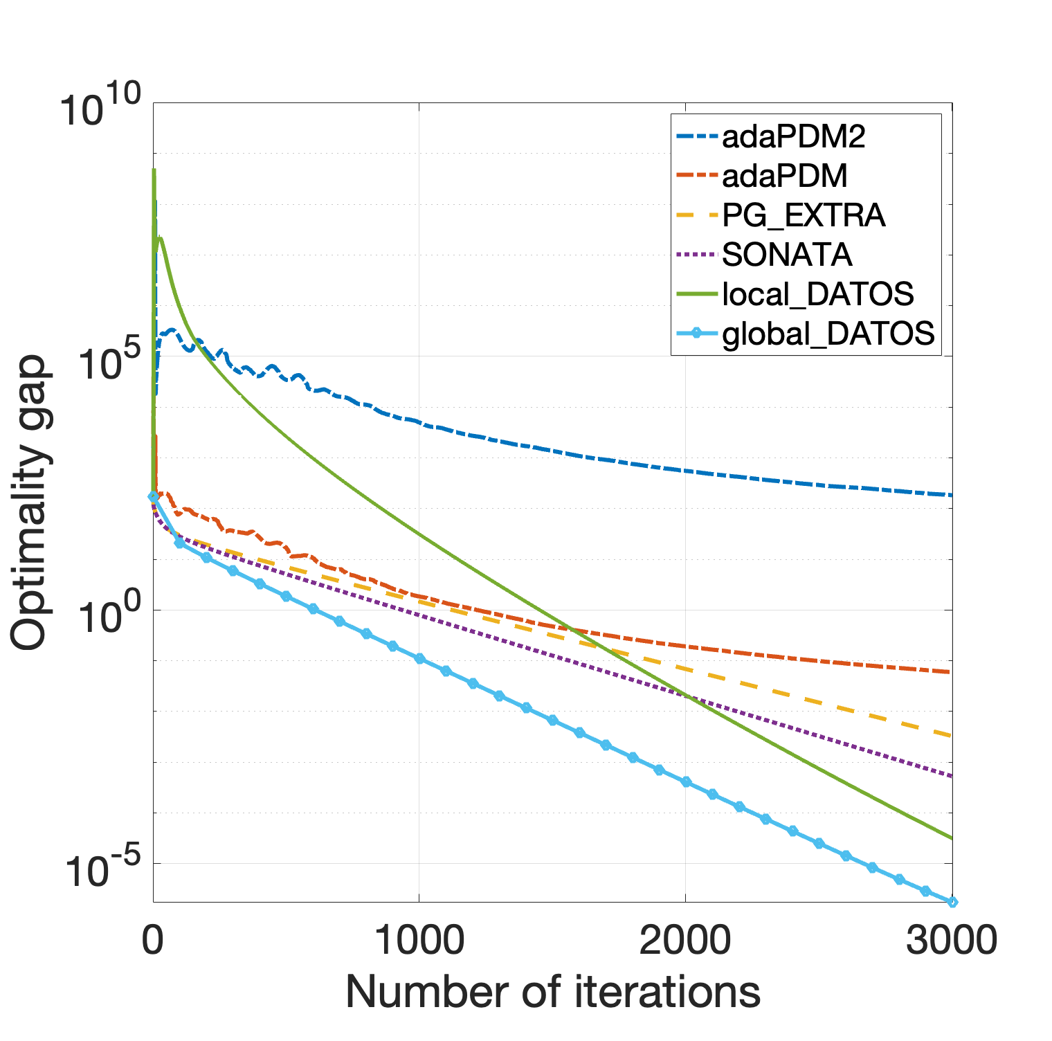
Figure 1 plots the optimality gap $({1}/{m})\sum_{i=1}^{m}u(x_{i})-u^{*}$ versus the number of iterations, achieved by all the algorihtms, where $u$ is the objective function in (P) and $u^{*}$ is its minimal value. The figures clearly show that both proposed methods consistently outperforms SONATA and PG-EXTRA, with the advantage that do not require any user’s intervention for the tuning of the stepsize. Moreover, our methods significantly outperforms also adaPDM in both of its implementations. Furthermore, the performance difference between Algorithm 3, which incorporates local-min consensus, and Algorithm 1–using global-min consensus, is remarkably negligible especially in networks with good connectivity.

IV-B Maximum likelihood estimate of the covariance matrix

Consider the decentralized estimation of the inverse of a covariance matrix, which is an instance of (P), with

$$f_{i}(X)=-n(\log(\texttt{det}(X)))-\texttt{trace}(XY_{i}),$$

and $r(X)=\delta_{C}(X)$, where $C=\{X\in\mathbb{S}^{d}_{++}:aI\preceq X\preceq bI\}$, for some $0<a\leq b$, and $Y_{i}=\frac{1}{n}\sum_{j=1}^{n}y_{j}^{i}(y_{j}^{i})^{\top}$ for $\{y_{j}^{i}\}$ being the set of local samples at agent $i$’s site, drawn by a Gaussian distribution with covariance matrix $\Sigma\in\mathbb{S}^{d}_{++}$. Here we take $n=100$ and $d=5$. Notice that this is a problem where the loss function $f$ is only locally smooth. Hence, SONATA and PG-EXTRA do not have theoretical convergence guarantees. We manually fine-tune their stepsizes for the best stable convergence behavior.

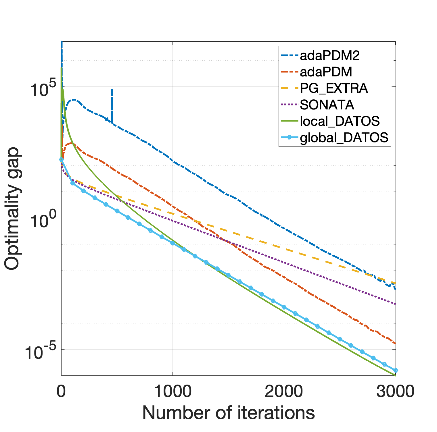
Figure 2 plots the optimality gap $({1}/{m})\sum_{i=1}^{m}u(x_{i})-u^{*}$ versus the number of iterations, achieved by all the algorihtms, where $u$ is the objective function in (P) and $u^{*}$ is its minimal value calculated by centralized proximal gradient method with linesearch, within the tolerance of $10^{-30}$. The figures clearly illustrate that both proposed methods consistently outperform SONATA and PG-EXTRA, which require conservative stepsize selections to ensure stable global convergence. Additionally, our methods surpass adaPDM in both considered variants. Notice that the iterates generated by Algorithm 3 remain bounded, due to the compactness enforced by $r(X)$.

IV-C Linear regression with elastic net regularization

We also report experiments solving a strongly convex non-smooth instance of Problem (P), with

$$f_{i}(x)=\frac{1}{n}\|A_{i}x-b_{i}\|^{2}+\frac{\gamma_{i}}{2}\|x\|^{2},\quad r(x)=\lambda\|x\|_{1},$$ (41)

where $(A_{i},b_{i})\in\mathbb{R}^{n\times d}\times\mathbb{R}^{n}$ are the data owned by agent $i$. The elements of $A_{i}$, $b_{i}$ are independently sampled from the standard normal distribution. Here, $n=20$ (hence $N=400$) and $d=500$. We set $\gamma_{i}=0.1+(i-1)\times 0.1$ and $\lambda=10^{-5}$, so that the smoothness parameter $L_{i}$ are different among each local function and the condition number of $f$ is $\kappa\approx 82.62$.

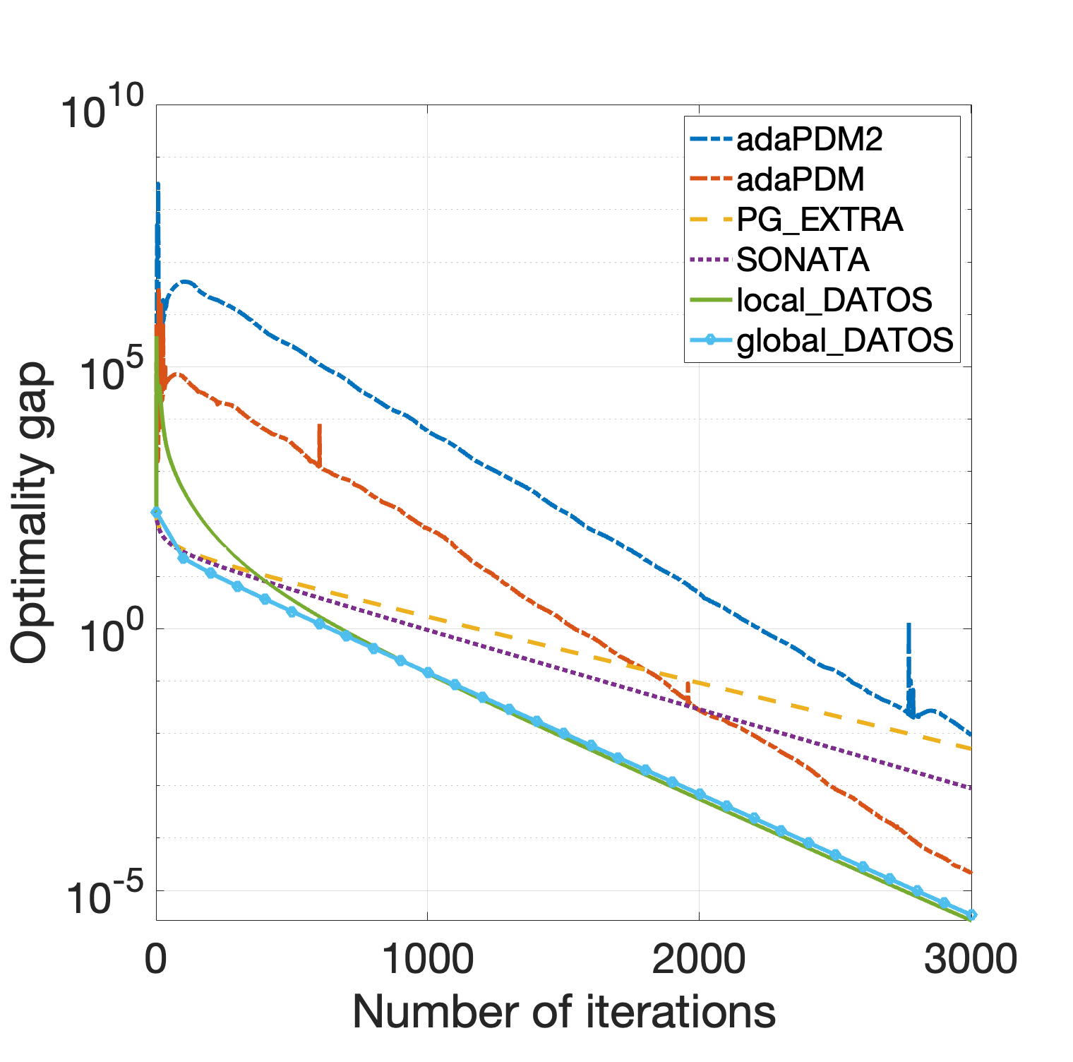
Figure 3 plots the optimality gap measured by $\|\mathbf{X}^{k}-\mathbf{X}^{*}\|^{2}$ versus the number of iterations. Similar to the convex scenario, both proposed algorithms clearly outperform existing decentralized benchmarks, particularly in poorly connected networks. Moreover, the results suggest that our methods exhibit (possibly asymptotic) linear convergence rates–an observation not captured by the theoretical analysis presented here. Theoretical support for this empirical behavior is provided in the extended version of the paper [36].

References

- [1] A. Nedić, A. Olshevsky, and M. Rabbat, “Network topology and communication-computation tradeoffs in decentralized optimization,” Proceedings of the IEEE, vol. 106, pp. 953–976, 2018.
- [2] A. H. Sayed, “Adaptation, learning, and optimization over networks,” Foundations and Trends in Machine Learning, vol. 7, pp. 311–801, January 2014.
- [3] D. P. Bertsekas, Nonlinear Programming. Athena Scientific, third ed., 2016.
- [4] D. O’Connor and L. Vandenberghe, “On the equivalence of the primal-dual hybrid gradient method and douglas–rachford splitting,” Mathematical Programming, vol. 179, no. 1, pp. 85–108, 2020.
- [5] B. Polyak, “Minimization of unsmooth functionals,” USSR Computational Mathematics and Mathematical Physics, vol. 9, no. 3, pp. 14–29, 1969.
- [6] J. Barzilai and J. M. Borwein, “Two-point step size gradient methods,” IMA Journal of Numerical Analysis, vol. 8, no. 1, pp. 141–148, 1988.
- [7] Y. Malitsky and K. Mishchenko, “Adaptive gradient descent without descent,” in International Conference on Machine Learning, 2019.
- [8] Y. Malitsky and K. Mishchenko, “Adaptive proximal gradient method for convex optimization,” arXiv preprint arXiv:2308.02261, 2024.
- [9] D. Zhou, S. Ma, and J. Yang, “Adabb: Adaptive barzilai-borwein method for convex optimization,” arXiv preprint arXiv:2401.08024, 2024.
- [10] J. Duchi, E. Hazan, and Y. Singer, “Adaptive subgradient methods for online learning and stochastic optimization,” in Proceedings of the 24th International Conference on Neural Information Processing Systems, pp. 257–265, 2011.
- [11] D. P. Kingma and J. Ba, “Adam: A method for stochastic optimization,” CoRR, vol. abs/1412.6980, 2014.
- [12] S. J. Reddi, S. Kale, and S. Kumar, “On the convergence of adam and beyond,” in International Conference on Learning Representations (ICLR), 2018.
- [13] A. Cutkosky and H. Mehta, “Momentum improves normalized SGD,” in Proceedings of the 37th International Conference on Machine Learning (H. D. III and A. Singh, eds.), vol. 119 of Proceedings of Machine Learning Research, pp. 2260–2268, PMLR, 13–18 Jul 2020.
- [14] X. Li and F. Orabona, “On the convergence of stochastic gradient descent with adaptive stepsizes,” in The 22nd international conference on artificial intelligence and statistics, pp. 983–992, PMLR, 2019.
- [15] R. Ward, X. Wu, and L. Bottou, “Adagrad stepsizes: Sharp convergence over nonconvex landscapes,” The Journal of Machine Learning Research, vol. 21, pp. 1–30, 2020.
- [16] S. Reddi, Z. B. Charles, M. Zaheer, Z. Garrett, K. Rush, J. Konečný, S. Kumar, and B. McMahan, “Adaptive federated optimization,” in International Conference on Learning Representations (ICLR), 2021.
- [17] X. Li, B. Karimi, and P. Li, “On distributed adaptive optimization with gradient compression,” in International Conference on Learning Representations (ICLR), 2022.
- [18] X. Chen, X. Li, and P. Li, “Toward communication efficient adaptive gradient method,” in Proceedings of the 2020 ACM-IMS on Foundations of Data Science Conference, (Virtual Event USA), p. 119–128, ACM, Oct. 2020.
- [19] P. Nazari, D. Tarzanagh, and G. Michailidis, “Dadam: A consensus-based distributed adaptive gradient method for online optimization,” IEEE Transactions on Signal Processing, vol. 70, p. 6065–6079, 2022.
- [20] X. Chen, B. Karimi, W. Zhao, and P. Li, “On the convergence of decentralized adaptive gradient methods,” in Asian Conference on Machine Learning, pp. 217–232, PMLR, 2023.
- [21] J. Li, X. Chen, S. Ma, and M. Hong, “Problem-parameter-free decentralized nonconvex stochastic optimization,” arXiv preprint arXiv:2402.08821, 2024.
- [22] I. Kuruzov, G. Scutari, and A. Gasnikov, “Achieving linear convergence with parameter-free algorithms in decentralized optimization,” Advances in Neural Information Processing Systems, vol. 37, pp. 96011–96044, 2024.
- [23] R. Aldana-Lopez, A. Macchelli, G. Notarstefano, R. Aragues, and C. Sagues, “Towards parameter-free distributed optimization: a port-hamiltonian approach,” arXiv preprint arXiv:2404.13529, 2024.
- [24] Y. Malitsky and T. Pock, “A first-order primal-dual algorithm with linesearch,” SIAM Journal on Optimization, vol. 28, no. 1, pp. 411–432, 2018.
- [25] P. Latafat, A. Themelis, and P. Patrinos, “Adaptive proximal algorithms for convex optimization under local lipschitz continuity of the gradient,” Mathematical Programming, Series A, 2024.
- [26] M. Bertero, P. Boccacci, G. Desiderà, and G. Vicidomini, “Image deblurring with poisson data: from cells to galaxies,” Inverse Problems, vol. 25, no. 12, p. 123006, 2009.
- [27] S. Boyd, N. Parikh, and E. Chu, Distributed optimization and statistical learning via the alternating direction method of multipliers. Now Publishers Inc, 2011.
- [28] H. H. Bauschke, J. Bolte, and M. Teboulle, “A descent lemma beyond lipschitz gradient continuity: first-order methods revisited and applications,” Mathematics of Operations Research, vol. 42, no. 2, pp. 330–348, 2017.
- [29] E. K. Ryu and W. Yin, Large-scale convex optimization: algorithms & analyses via monotone operators. Cambridge University Press, 2022.
- [30] D. Davis and W. Yin, “A three-operator splitting scheme and its optimization applications,” Set-valued and variational analysis, vol. 25, pp. 829–858, 2017.
- [31] D. Kim, J. Lim, and J. Kim, “Low-power, long-range, high-data transmission using wi-fi and lora,” in 2016 6th International Conference on IT Convergence and Security (ICITCS), (Prague, Czech Republic), p. 1–3, IEEE, Sept. 2016.
- [32] T. Janssen, N. BniLam, M. Aernouts, R. Berkvens, and M. Weyn, “Lora 2.4 ghz communication link and range,” Sensors, vol. 20, p. 4366, Aug. 2020.
- [33] A. Chambolle and T. Pock, “A first-order primal-dual algorithm for convex problems with applications to imaging,” Journal of mathematical imaging and vision, vol. 40, pp. 120–145, 2011.
- [34] W. Shi, Q. Ling, G. Wu, and W. Yin, “A proximal gradient algorithm for decentralized composite optimization,” IEEE Transactions on Signal Processing, vol. 63, no. 22, pp. 6013–6023, 2015.
- [35] L. Guo, X. Shi, J. Cao, and Z. Wang, “Decentralized inexact proximal gradient method with network-independent stepsizes for convex composite optimization,” IEEE Transactions on Signal Processing, vol. 71, pp. 786–801, 2023.
- [36] X. Chen, I. , Kuruzov, G. Scutari, and A. Gasnikov, “Adaptive decentralized algorithms for composite convex optimization,” in preparation, 2025.
- [37] Y. Sun, G. Scutari, and A. Daneshmand, “Distributed optimization based on gradient-tracking revisited: Enhancing convergence rate via surrogation,” SIAM J. on Optimization, vol. 32, pp. 354–385, 2022.
- [38] C. Chih-Chung, “” libsvm: a library for support vector machines,” acm transactions on intelligent systems and technology, 2: 27: 1–27: 27, 2011,” http://www. csie. ntu. edu. tw/˜ cjlin/libsvm, vol. 2, 1996.