Superradiance Constraints from GW231123

Abstract

Gravitational wave observations have recently revealed with high significance, and high precision, the existence of $\mathcal{O}(100)\,M_{\odot}$ rapidly rotating black holes, allowing gravitational wave events to be used for the first time to probe unexplored axion parameter space using the phenomenon known as black hole superradiance. Here, we present new limits on axions using the binary black hole merger event GW231123, whose constituent black holes are among the fastest spinning observed with gravitational waves to date. We demonstrate that the most viable binary formation channels lead to conservative constraints on axion masses $\mu\sim[0.6-5]\times\,10^{-13}$ eV and decay constants $f_{\Phi}\gtrsim 10^{14}$ GeV, extending existing superradiance constraints derived using x-ray observations to yet lower axion masses.

I Introduction

The LIGO-Virgo-KAGRA (LVK) collaboration has recently announced the detection of the merger of two constituent BHs (BHs) with masses $M_{1}=137^{+22}_{-17}\,M_{\odot}$ and $M_{2}=103^{+20}_{-52}\,M_{\odot}$ (at $90\%$ credible intervals) [1]. From an astrophysical perspective, this event is remarkable, as the inferred masses of both constituents lie in the so-called “pair instability mass gap” [2, 3, 4] (i.e. the range of masses in which pair instabilities prevent the formation of BHs directly from stellar collapse) and represent the heaviest high-significance gravitational wave (GW) event observed to date [5, 6]. This event is even more interesting from the perspective of a particle physicist, as there is a strong preference in the waveform that at least one, if not both, constituent BHs have extremely high dimensionless spin, $\tilde{a}_{1}=0.90^{+0.10}_{-0.19}$ and $\tilde{a}_{2}=0.80^{+0.20}_{-0.51}$, with the primary exhibiting the highest black hole spin ever confidently measured through GWs. This unprecedented measurement is obtained thanks to the confident inference of a large effective precessing spin [7], a feature which appears robust against waveform systematics [1]. This is significant as it represents the first time GW data can be used to probe unexplored parameter space of new light fundamental bosonic particles via the phenomenon known as superradiance.

Figure 1: Constraint on the axion decay constant $f_{\Phi}$ and mass $\mu$ derived from GW231123 (blue); result is obtained using NRSur waveform model analysis, using $N_{\rm max}=5$, and with $\tau_{\rm max}=10^{5}$ (shaded), $10^{6}$ (dashed), and $10^{7}$ years (dot-dashed). Shown for comparison are superradiance constraints on solar-mass scale BHs [8], with spin inferences performed using x-ray data (black), the QCD axion line (red), and the parameter space where misalignment mechanism could produce the entirety of dark matter with $\mathcal{O}(1)$ initial field values (green). The inverse Planck scale $M_{\rm Pl}$ is highlighted with a horizontal dashed line.

BH superradiance is a phenomenon in which low-energy bosonic fields experience an instability around Kerr BHs, causing them to rapidly transfer the rotational energy of the BH into high-occupation number quasi-bound states (see e.g. [9] for a review). For a scalar field, this process, under optimal circumstances, can lead to an order one depletion of the BH spin on the timescale of hours [10, 11, 12, 13, 14, 15, 16], suggesting an inherent incompatibility between rapidly rotating BHs and the existence of light bosons [17, 18, 19, 20, 21].

To date, superradiance constraints have been derived using BH spin measurements that are inferred from x-ray observations [22, 23, 24, 25, 8]; this approach, however, can be highly sensitive to the properties of matter near the innermost stable circular orbit (where the modeling is the least well-understood), the details of radiative transfer, and the thermodynamic properties of x-ray emitting regions – see e.g.  [8] for a detailed discussion of systematics. GW observations offer an alternative route to measuring high-spin BHs which is free from the modeling systematics that plague x-ray observations – the only difficulty, until now, has been the lack of gravitationally-observed high-spin BHs.

The aim of this Letter is to demonstrate the power of GW231123, and more generally the power of forthcoming GW observations, in using spin measurements to constrain the existence of light bosonic particles. We focus specifically on the extent to which the inferred spin distributions of the constituent BHs in GW231123 can be used to probe axions, as these particles constitute the most well-motivated bosons at low energies (we do, however, derive a constraint on non-interacting spin-1 fields in Supplemental Material, which includes Refs. [31, 32, 33, 34, 35, 36, 37, 38, 39, 40, 41, 42, 43, 44, 45, 46, 47, 48, 49, 50, 51, 52, 53, 54, 55, 56, 57, 58, 59, 60, 61, 62, 63, 64, 65, 66, 67, 68, 69, 70, 71, 72, 73, 74, 75, 76, 77, 78, 79, 80, 81, 82, 83]). Using the inferred properties of GW231123, we deduce the range of characteristic timescales over which superradiance could have spun down the BHs, within realistic assumptions motivated by the hierarchical formation scenario (see e.g. [84] for a review). We then use the inferred posteriors on the spin of each constituent BH, along with motivated priors on their natal values, to simulate possible spin-down histories in the presence of an axion. The main result of this paper is the limit shown in Fig. 1, which demonstrates that GW231123 has excluded a new, and well-motivated, region of axion parameter space that is effectively inaccessible to conventional searches. Needless to say, the constraints derived here rely on the inferred spins of the constituent BHs in GW231123; while the inference of high spins appears to be robust to variations in waveform modeling, the spin posteriors are still sensitive systematic uncertainties that can induce small shifts into the inferred limits (we note, however, that the sensitivity is primarily affected by the small-spin region of the posterior – see Supplemental Material A). As waveform modeling improves in the future, so too will the robustness of these constraints; in addition, the approach and methodology used in the analysis here will undoubtedly prove invaluable as new detections of high-spin BHs emerge.

II Black Hole Superradiance

Let us start with a brief review of BH superradiance. Here, we restrict our attention to scalar fields – generalizations to the case of higher spin fields can be found e.g. in [89, 90, 91, 92, 93, 13, 12, 94, 95, 96, 15, 97, 9] (in Supplemental Material  D, we also estimate constraints on non-interacting spin-1 fields). We focus specifically on the case of axions $\Phi$, i.e. light pseudoscalars which have an intrinsic discrete shift symmetry $\Phi\rightarrow\Phi+2\pi f_{\Phi}$ that protects the smallness of the mass, where $f_{\Phi}$ is the axion decay constant. The existence of the shift symmetry implies contributions to the axion potential are of the form $V(\Phi)=\mu^{2}f_{\Phi}^{2}\left[1-\cos\left(\frac{\Phi}{f_{\Phi}}\right)\right]+\cdots$ (with higher order, shift-symmetry preserving terms, potentially being present), which for small field values reduces to $V(\Phi)\simeq\frac{1}{2}\,\mu^{2}\,\Phi^{2}-\frac{1}{4!}\lambda\Phi^{4}+\cdots$, with $\mu$ the axion mass, and $\lambda\equiv(\mu/f_{\Phi})^{2}$. Thus, a natural expectation of axions is the existence of quartic self-interactions; despite a very small coupling constant, this interaction plays an important role in the evolution of superradiant systems [18, 98, 99, 100, 101, 24, 102, 8].

The evolution of superradiant states can be determined by solving the equation of motion in a Kerr background. At leading order, one can neglect self-interactions and solve for the complex energy spectrum of quasi-bound states near the black hole; this energy spectrum is discrete, with eigenvalues $\omega=\omega_{r}+i\Gamma$ labeled by a set of quantum numbers $\left|n\ell m\right>$, see e.g.  [10, 103, 14]; these quantum numbers are analogous to the principal $n$, orbital $\ell$, and magnetic $m$ quantum numbers of the hydrogen atom, obeying $n\geq\ell+1$, $\ell\geq 0$, and $|m|\leq\ell$. The fastest growing state is the $\left|211\right>$, which for a $\mathcal{O}(100)\,M_{\odot}$ BH has an $e-$fold growth timescale that can be as short as $\tau_{211}\equiv(2\Gamma_{211})^{-1}\sim\mathcal{O}({\rm hours})$. For a free particle, the growth of the state saturates when the angular frequency of the horizon $\Omega_{H}$ reaches a value $\Omega_{H}\equiv\tilde{a}/(2r_{+})\sim\mu/m$ , where $\tilde{a}\equiv a/(GM)$ is the dimensionless spin and $r_{+}=GM(1+\sqrt{1-\tilde{a}^{2}})$ is the outer horizon. This requires roughly $\mathcal{O}(180)$ e-folds of growth, implying the spin of a rapidly rotating BH can be modified on timescales of days. In the calculations below, we compute the eigen-frequencies of each state and at each point during spin-down using the continued fraction method [104, 105, 106, 11].

Self-interactions serve to coupled the different eigenstates of the system, transferring energy efficiently between them . Rather than having decoupled growth of quasi-bound states, as in the case of the free particle solution, self-interactions induced coupled evolution of states in which the growth of any state can be quenched, saturating to a fixed occupation number, long before altering the spin of the BH [101, 24, 102, 8]. The evolution of the superradiant system can be determined by following the energy injection and dissipation, which is described by the set of equations:

$$\dot{\epsilon}_{n\ell m} = 2\Gamma_{n\ell m}\,\epsilon_{n\ell m}+\sum_{\mathcal{R}_{i,j,k}}\,\zeta_{i,j}\,\gamma_{i,j}^{k,{\rm L}}\,\epsilon_{i}\,\epsilon_{j}\,\epsilon_{k}$$ (1)

$$\dot{\tilde{a}} = -\sum_{n\ell m}2\,m\,\Gamma_{n\ell m}\,\epsilon_{n\ell m}$$ (2)

$$\frac{\dot{M}}{\mu GM^{2}} = -\sum_{n\ell m}2\Gamma_{n\ell m}\,\epsilon_{n\ell m}+\sum_{(i,j,k)}\gamma_{i,j}^{k,{\rm BH}}\,\epsilon_{i}\,\epsilon_{j}\,\epsilon_{k}\,.$$ (3)

where $\epsilon_{n\ell m}\equiv N_{n\ell m}/(GM^{2})$ is the normalized occupation number $N_{n\ell m}$ of a state, $\zeta_{i,j}$ is a degeneracy counting factor equal to 1 for $i\neq j$ and 2 for $i=j$. Here, we have introduced rate coefficients $\gamma_{i,j}^{k,{\rm L}}$, where the indices $(i,j,k)$ denote quasi-bound states (i.e. $i=\left|n\ell m\right>$, $j=\left|n^{\prime}\ell^{\prime}m^{\prime}\right>$, etc), and ‘L’ represents energy loss, either to infinity $\infty$ (occurring when $\omega_{i}+\omega_{j}-\omega_{k}>\mu$), or into bound states which dissipate their energy into the BH (occurring when $\omega_{i}+\omega_{j}-\omega_{k}\leq\mu$). The collective list of non-zero scattering rates relevant for $n\leq 5$ is presented in Table 1 and 2 of [8]. Note that the axion mass implicitly enters in both the eigenvalues $\Gamma_{n\ell m}$ as well as the scattering rates $\gamma_{i,j}^{k,L}$, while the decay constant enters only through the scattering rates.

In general, one should include all states that obtain non-negligible occupation numbers on the timescales of interest; in practice, however, this is currently unfeasible, with the latest analyses only including states with $n\leq 5$ [8]. Here, we perform our fiducial analysis with all states $n\leq 5$, and illustrate the impact of taking instead $n\leq 3$ in the Supplemental Material. All rate coefficients are computed using the procedure of [8].

In solving Eqns. 1-3, there is an important subtlety which arises from the fact that we observe the spin and mass close to the merger, and these values may differ sizably from those at birth. For this reason, one typically evolves the superradiant system on timescales $t\lesssim\tau_{\rm max}$, where $\tau_{\rm max}$ is chosen to be sufficiently short that astrophysical processes cannot appreciably alter the mass or spin of the system; for isolated BHs, this is often taken to be the Salpeter timescale, $\tau_{\rm Salp}\sim 4.5\times 10^{7}$ yr, however we argue in the following Section that for GW231123 the relevant timescale may be shorter, and thus we apply adopt a more conservative timescale in our analyses. In general, one could attempt to model the evolution on longer timescales, including e.g. accretion, multiple mergers, etc. [117], but this requires complicated astrophysical modeling which is beyond the scope of this work.

III Determination of Merger Timescales

As mentioned in the preceding section, testing superradiance typically requires defining the characteristic timescale over which the properties of the black hole can be assumed to remain constant. For isolated black holes, this is often taken to be the Salpeter timescale. For second or third generational hierarchical mergers, the relevant timescale is instead determined by the time between successive mergers, $\tau_{\rm merger}$, which can be significantly shorter than $\tau_{\rm Sal}$. Since the large masses and spins of the BHs involved in the GW231123 event strongly suggest that one or both of the binary components may be the product of a previous binary BH merger [1, 118, 119], a scenario known as a hierarchical merger [120, 121, 122, 123, 124, 125, 126, 127, 128, 129, 130, 131, 122, 132, 133] (see e.g. [84] for a review), we endeavor to determine the minimal value of $\tau_{\rm merger}$ consistent with the properties of GW231123. In App. B we further discuss more exotic scenarios, showing the constraint in Fig. 1 remains valid.

Assuming a hierarchical origin, one can infer important information about the general properties of the local environment. For instance, the presence of high-spin BHs in GW231123 is consistent with significant anisotropic GW emission, which implies large recoil velocities for the remnants of first-generation mergers which constitute the progenitors of GW231123—typically on the order of several hundred kilometers per second [134]. If this “birth kick” exceeds the escape velocity of the host environment, further mergers would be prevented. This suggests that GW231123 likely originated in a deep potential well, e.g. in a nuclear star cluster (NSC) [132, 122, 135, 136, 137, 138, 139] or an active galactic nucleus (AGN) [140, 141, 142, 143, 144, 145, 146, 147, 148, 149, 150, 151], where escape velocities can reach $v_{\rm esc}\sim 100$–$500~\mathrm{km/s}$ or higher. In contrast, typical escape velocities from young stellar clusters and globular clusters are significantly lower, $v_{\rm esc}\lesssim 50~\mathrm{km/s}$ [152, 153, 154], making it unlikely that the remnants of earlier mergers could have been retained in such environments.

In general, one can write the rate density of BH-BH mergers as

$$\mathcal{R}=n_{\rm env}N_{\rm BH}(M_{\rm BH})\Gamma_{\rm merger},$$ (4)

where $n_{\rm env}$ is the average number density in the Universe of the environment under consideration, $N_{\rm BH}$ is the number of BHs within such an environment (where we included explicitly the dependence on the BH mass), and $\Gamma_{\rm merger}$ is the merger rate per BH. Such a rate can be decomposed into two contributions, $\Gamma_{\rm merger}\sim\frac{1}{\tau_{\rm pair}+\tau_{\rm coal}}$, where $\tau_{\rm pair}$ is the pairing timescale for two BHs, and $\tau_{\rm coal}$ is the time to coalescence once the binary has formed. In what follows, we will assume the former dominates the merger timescales and that the coalescing time is negligible. This is particularly justified for GW231123 which is expected to form from dynamical processes involving large velocity BHs. In fact, one can verify that for the parameters of interest, namely $v\sim v_{\rm recoil}\gtrsim 100\,\text{km/s}$, $\tau_{\rm pair}\gg\tau_{\rm coal}$, where $v$ denotes the relative velocity of a BH pair and $v_{\rm recoil}$ represents the “birth-kick” recoil velocity of the remnants from first-generation mergers. Such a hierarchy is naturally expected, as both the binary formation rate (scaling as $\tau_{\rm pair}\propto v^{11/7}$ for dynamical capture [155, 147], and $\tau_{\rm pair}\propto v^{9}$ for three-body formation [156, 157]) and the coalescing time (scaling as $\tau_{\rm coal}\propto v^{-36/7}$ for dynamical capture, and $\tau_{\rm coal}\propto v^{-8}$ for three-body formation, assuming Peter’s formula [158, 159]) scale strongly with $v$. A similar argument applies to other channels, such as e.g. binary-single interactions. We will proceed under this assumption, which allows us to treat superradiance growth around both individual isolated BHs (see Supplemental Material for a discussion on the impact of the binary), before they pair in the binary and merge soon after.

The rate density in Eq. 4 should then be compared with the one inferred by the LVK collaboration for GW231123, $\mathcal{R}_{\rm obs}=0.08^{+0.19}_{-0.07}~\mathrm{Gpc}^{-3}~\mathrm{yr}^{-1}$. From such a comparison, one can infer the characteristic pairing time,

$$\tau_{\rm pair}\simeq\tau_{\rm merger}\equiv\Gamma_{\rm merger}^{-1}=\frac{n_{\rm env}N_{\rm BH}(M_{\rm BH})}{\mathcal{R}_{\rm obs}}.$$ (5)

This estimate is fully agnostic with respect to the physical mechanisms responsible for binary formation and coalescence. In order to provide realistic numbers, we will evaluate Eq. 5 considering at least one of the BHs to be a remnant, and treating separately the possibility that this event occurred in an AGN or NSC.

III.1 Active galactic nuclei

In AGN, gas-rich accretion disks surround supermassive BHs, and stellar-mass BHs can become embedded and experience migration due to torques from the surrounding gas [148]. A particularly relevant feature of AGN disks is the presence of migration traps—locations where the net torque acting on an object vanishes, halting its inward or outward drift [160]. These traps naturally concentrate compact objects, enhancing the probability of dynamical interactions and subsequent mergers, making AGN disks ideal for multiple merger generations. As such, they offer a promising, natural scenario for explaining the high-spin, hierarchical nature of events like GW231123.

In this environment, the merger timescale in Eq. 5 is

$$\tau_{\rm merger}^{\rm AGN} =\text{Myr}\left(\frac{n_{\rm env}^{\rm AGN}}{10^{-5}\,\text{Mpc}^{-3}}\right)\left(\frac{N_{\rm BH}}{10}\right)$$

$$\times\left(\frac{0.1\,\mathrm{Gpc}^{-3}~\mathrm{yr}^{-1}}{\mathcal{R}_{\rm obs}}\right),$$ (6)

where for the AGN number density at low redshift ($z\lesssim 0.5$), we adopted a typical, yet conservative, value inferred from multi-wavelength luminosity functions (see, e.g., Fig. 7 in Ref. [161]). This number density only includes contributions from AGN with luminosities within the range where migration traps are expected to form and persist [129]. The number of massive, second-generation BHs in the trap is instead estimated following Ref. [162] (see their Fig. 9), where the authors simulate first-generation BH mergers embedded in the AGN disk and track their migration, binary pairing, and mergers. We stress that if the number of BHs is larger than expected, for a fixed observed rate, this would imply a larger merger timescale and therefore one could probe a larger region of the axion parameter space. We also note that the observed rate, $\mathcal{R}_{\rm obs}$, ranges from $0.01$ to $0.3\;\mathrm{Gpc}^{-3}\,\mathrm{yr}^{-1}$ at $90\%$ C.L., implying that $\tau_{\rm pair}$ could be smaller by a factor of a few, or alternatively up to ten times longer. Overall, adopting

$$\tau_{\rm merger}^{\rm AGN}\sim 10^{-1}\text{--}10\;\mathrm{Myr}$$ (7)

should abundantly encompass all uncertainties.

III.2 Nuclear star clusters

NSCs [163] represent an alternative dynamical environment in which compact-object binaries can form and merge multiple times. Compared to AGN disks, NSCs are gas-poor systems, but they can nonetheless sustain high merger rates due to their large stellar densities and deep gravitational potentials. The dominant binary formation mechanism in NSCs depends on whether or not a central supermassive BH (SMBH) is present. In NSCs that do host an SMBH, the short relaxation time facilitates the development of a steep density cusp of stellar-mass BHs around the central object, enhancing the probability of binary formation via gravitational-wave capture [147]. In contrast, NSCs without a SMBH behave more like high-mass globular clusters, where binaries form and harden primarily through three-body encounters and binary single interactions [121]. In either case, we can write an expression for the merger rate analogous to that in Eq. 4.

The number density of NSCs in the local universe, relevant for events like GW231123, whose redshift is $z=0.39^{+0.27}_{-0.24}$, depends on the fraction of galaxies that host NSCs and on the galaxy stellar mass function. The former peaks at approximately 90% for galaxies with a stellar mass around $\sim 10^{9}\,M_{\odot}$, and decreases toward both higher and lower masses. Nonetheless, nucleation fractions remain at the level of $\sim 10\%$ even for galaxies as small as $M_{*}\sim 5\times 10^{5}\,M_{\odot}$ and as massive as $M_{*}\sim 5\times 10^{11}\,M_{\odot}$ (see Fig. 3 of Ref. [164]). Each galaxy can host at most one NSC, located at its photometric and dynamical center (unlike the case for globular clusters). This allows us to estimate $n_{\rm env}^{\rm NSC}\sim n_{\rm gal}f_{\rm NSC}$. Using results from galaxy stellar mass function studies [165, 166, 167], and adopting a conservative value of $f_{\rm NSC}\sim 10\%$, we obtain (see also [135]) $n_{\rm env}^{\rm NSC}\sim 10^{-3}\,\mathrm{Mpc}^{-3}$.

As in the case of AGN, determining $N_{\rm BH}(M_{\rm BH})$ is less straightforward, but we can expect it to be in the same ballpark. In fact, assuming standard stellar initial mass functions [168], one expects $0.1-1\%$ of the NSC mass to be in the form of seed BHs that may form binaries and merge [169, 170]. Typical NSC have masses $\sim 10^{5}-10^{8}\,M_{\odot}$, which implies roughly $M_{\rm BH,tot}\sim 10^{3}-10^{4}\,M_{\odot}$. Of these BHs, we can expect $10-50\%$ of them to be in binaries [171]. The majority of these BH will on average have masses $\sim 10-20\,M_{\odot}$, leaving us with $\sim\mathcal{O}(10-100)$ BHs which will then undergo repeated mergers. We can thus write

$$\tau_{\rm merger}^{\rm NSC}=10\,\text{Myr}\,N_{\rm BH}\left(\frac{n_{\rm env}^{\rm NSC}}{10^{-3}\,\text{Mpc}^{-3}}\right)\left(\frac{0.1\,\mathrm{Gpc}^{-3}~\mathrm{yr}^{-1}}{\mathcal{R}_{\rm obs}}\right)\,,$$ (8)

implying

$$\tau_{\rm merger}^{\rm NSC}\sim 1\text{--}100\;\mathrm{Myr}$$ (9)

should bracket all uncertainties.

IV Analysis and Conclusions

Here, we begin by providing a heuristic description of our statistical framework that allows one to derive constraints on the axion parameter space; a statistically rigorous derivation of the relevant quantities from the LVK posterior is also included for completeness.

First, we fix the axion mass; this is useful as our posterior will otherwise be unbounded in three directions (and thus risks having a high sensitivity to the prior). We adopt a log-flat prior on $f_{\Phi}$ over the range $[10^{11},10^{20}]\,\mathrm{GeV}$. We focus on understanding the evolution of the BHs from a time $t=t_{\rm 0}-\tau_{\rm max}$, to the time of merger $t_{\rm 0}$, as uncertainties in the merger history do not allow us to infer the properties of the BHs on longer timescales. In our analysis, we vary $\tau_{\rm max}$ to be consistent with the shortest characteristic timescales identified in the viable formation channels associated with NSCs and AGNs, with our fiducial limits taken to be the minimum of these, namely $10^{5}$ years. Since the change in mass of each BH due to superradiance is small relative to the mass uncertainty, one can account for the mass measurement by adopting mass priors using the LVK joint prior distribution $p(M_{1},M_{2})$. The initial spins at a time $t=t_{\rm 0}-\tau_{\rm max}$ are, of course, unknown – while astrophysical processes cannot alter the spins on these timescales, superradiance can. Since superradiance only serves to extract spin, we adopt spin priors which contain non-zero weight only above the inferred values of the spins at merger. More specifically, given a sample $i$ of the $X=1,2$ BH (with $`1^{\prime}$ corresponding to the heavier BH), we compute the conditional distribution $p(\tilde{a}_{X}|M_{1,i},M_{2,i})$; we then determine the mean $\zeta_{X}$ and standard deviation $\beta_{X}$ in the conditional probability $p(\tilde{a}_{X}|M_{1,i},M_{2,i})$ (which we infer from the LVK posterior), and adopt a prior that is half-flat, for $\tilde{a}_{X,i}>\zeta_{X}$, and half-Gaussian, for the initial spin $\tilde{a}_{X,i}\leq\zeta_{X}$. The half-Gaussian distribution ensures an appropriate sampling of the initial spin distribution in the event that superradiance does not spin down the black hole, while the half-flat component of the prior ensures that initial high-spin black holes which have been spun down via superradiance to $\tilde{a}=\left<\tilde{a}_{X}\right>$ are perfectly compatible with the observed data. Eqns. 1-3 are then evolved from $t=t_{\rm 0}-\tau_{\rm max}$ to $t=t_{\rm 0}$, to determine the spins that would have been observed by LVK $\tilde{a}_{1,2}$ at merger. In order to evaluate the compatibility of the predicted spins with those observed, we construct a likelihood using two-dimensional kernel density estimation (KDE) on the set of conditioned posterior samples $p(\tilde{a}_{1},\tilde{a}_{1}|M_{1,i},M_{2,i})$ from the LVK analysis. The interested reader can find a more detailed derivation of the statistical procedure in the Supplemental Material.

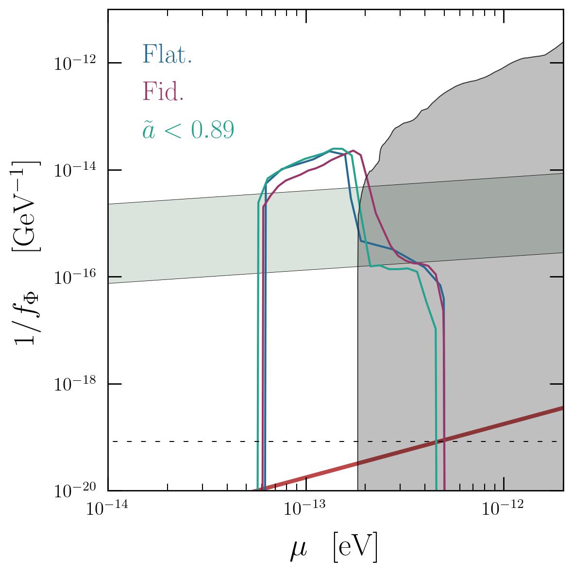
We run between five and ten Monte Carlo chains, reconstruct the one dimensional marginalized posterior on $f_{\Phi}$ from the Monte Carlo samples, and extract the $90\%$ lower limit. This procedure is repeated over many axion masses, and the collection of these points produces the limit shown in Fig. 1. Note the multi-bump feature is driven primarily by the contributions of the heavier (left) and lighter (right) BHs (while multi-bumped features do also arise from the presence of different superradiant states for single BHs, the $\left|322\right>$ state of the heavy BH is sub-dominant to the $\left|211\right>$ state of the light BH at higher axion masses). For reference, we also show in Fig. 1 superradiance constraints (gray) derived using x-ray observations [8], the values of $f_{\Phi}-\mu$ corresponding to the QCD axion (red), and the parameter space where the misalignment mechanism can most naturally generate the dark matter abundance (green). Note that the limit derived in Fig. 1 contains sensitivity to both black holes (see Supplemental Material). The various features seen in the limit arise from the interplay of having BHs of different masses, and looking at the spin-down induced by the $m=1$ and $m=2$ states.

This analysis demonstrates that GW observations of high-spin BHs can be used to set competitive limits on axions (and, more generally, light bosonic fields) in unexplored regions of the parameter space. The dominant uncertainty entering this analysis comes from the unknown timescale between successive mergers of the constituent BHs – this is in contrast to approaches using x-ray observations, where the dominant systematic arguably comes from the modeling of the accreting material near the horizon. Using a data-driven approach, we have argued that this uncertainty is not prohibitive, and that GW231123 can be used to derive meaningful constraints on feebly coupled axions.

The upcoming high-sensitivity LVK O5 run [175] promises to significantly enhance discovery potential for similar events. Thanks to an expected signal-to-noise ratio improvement of ${\cal O}(3)$ [176], the observable volume will expand by nearly ${\cal O}(20)$. The detection of additional events of this kind in future LVK runs would be accompanied by narrower uncertainties on event parameters and will allow for improved constraints on the underlying spin distribution, along with other source population properties, thereby strengthening the bounds discussed in this work.

V Acknowledgments

The authors would like to thank Giovanni Maria Tomaselli, Paolo Pani, Enrico Barausse, and Davide Gerosa for their useful comments. AC is supported by an ERC STG grant (“AstroDarkLS”, grant No. 101117510). SJW acknowledges support from a Royal Society University Research Fellowship (URF-R1-231065). This work is also supported by the Deutsche Forschungsgemeinschaft under Germany’s Excellence Strategy EXC 2121 “Quantum Universe” 390833306. This article/publication is based upon work from COST Action COSMIC WISPers CA21106, supported by COST (European Cooperation in Science and Technology). The data that support the findings of this article are openly available [177].

In the following, we show the results of our analysis adopting different posterior samples, likelihoods, and merger time-scales. We also discuss more exotic scenarios for GW231123, provide a comprehensive outline of the statistical procedure adopted, discuss the impact of binary systems on the evolution of superradiant clouds, and derive constraints on non-interacting spin-1 bosons.

Appendix A Additional Results

For the sake of completeness, we show how our limits vary when adopting different assumptions in the underlying analysis. The fiducial analysis shown in the main text has been performed using the NRSur posterior samples from the LVK collaboration [31], taking $\tau_{\rm max}=10^{5},10^{6},$ and $10^{7}$ years. In Fig. 2 we compare the impact of instead adopting posterior samples from the ‘combined’ analysis (which combines samples from five BH waveform models, of which one is the NRSur model); this is done using maximum timescales of $\tau_{\rm max}=10^{6}$ and $10^{7}$ years. We observe small differences in the resulting limits depending on the posterior samples used in the analysis, but primarily for masses $\mu\gtrsim 2\times 10^{-13}$ eV.

We also compare the impact of running our analysis with either $N_{\rm max}=5$, or $N_{\rm max}=3$. The equivalent of Fig. 1, but fixing $N_{\rm max}=3$, is shown in the left panel of Fig. 3, while in the right panel of Fig. 3 we fix $\tau_{\rm max}=10^{6}$ years, and we show the results for both waveform analyses with $N_{\rm max}=3,5$.

Next, we look at the relative importance of including both black holes in the analysis. We plot in Fig. 4 the limits derived using the correlated mass-spin information on both BHs, versus using only the heavier, more prominently measured, BH. This is done for $N_{\rm max}=3$ and $\tau_{\rm max}=10^{6}$ years (left), and for $N_{\rm max=5}$ and $\tau_{\rm max}=10^{5}$ years (right). For masses $\mu\sim 2\times 10^{-13}$ eV, the $\left|211\right>$ state is not fully efficient at spinning down the heavy BH; however, samples which are consistent with $\tilde{a}_{1}\sim 0.75$ inherently imply that $\tilde{a}_{2}$ is large, and thus the contribution from the second BH to the likelihood becomes significant.

Finally, we look at the sensitivity of our derived limit to the high-spin component of the prior. Since the NRSur likelihood is not calibrated for spins $\tilde{a}\gtrsim 0.89$, we truncate the prior to remove spins above this threshold. The result of performing this analysis, using $N_{\rm max}=3$ and $\tau_{\rm max}=10^{5}$ years, is shown in Fig. 5. Here, one sees that the constraints are actually strengthened at low masses, and weakened at high masses. This result is as expected. For low mass axions, the $\left|211\right>-\left|322\right>$ states are in an equilibrium with suppressed occupation numbers, and thus larger initial spins require longer timescales in order to reach the lower edge of the spin posterior. For high masses, the $\left|322\right>$ state grows unimpeded, and thus one recovers the non-interacting result in which most of the time spent growing the cloud, rather than spinning down the black hole, and thus higher spins (which correspond to faster growth timescales) lead to stronger constraints. This result indicates that our derived sensitivity errors on the side of conservative, even though there are large uncertainties in the NRSur likelihood at $\tilde{a}\gtrsim 0.89$. In order to provide an illustrative example, we also show a few of the one-dimensional posterior distributions on $f_{a}$ in Fig. 6.

Note that Ref. [178] appeared online at the same time as this work, and also used GW231123 to place constraints on new bosons from superradiance. The constraints on $f_{\Phi}$ derived in  [178] are somewhat weaker than those derived here. Part of this discrepancy comes from the fact that they only used the more massive BH in their analysis – Fig. 4 suggests that this likely leads to a sizable difference for axion masses $\mu\gtrsim 10^{-12}$ eV. In addition, we note that the analysis of  [178] does not explicitly time-evolve the system, but rather imposes a constraint by comparing posterior spin samples with the maximum allowed spin of a fully evolved state. For a non-interacting boson, the system evolves exponentially fast, and thus this introduces only a small error; for self-interacting axions, however, this approach can produce overly conservative limits, often by a factor of a few (see [8] for a discussion). Finally, we note that our fiducial analysis includes $N=4,5$ states, allowing us to extend our analysis to large axion masses.

Appendix B Alternative Scenarios

In this section, we explore more exotic hypotheses for the origin of the GW231123 event and assess the robustness of the constraints presented in Fig. 1. We critically examine alternative formation channels beyond the most plausible hierarchical scenario and evaluate the extent to which our conclusions remain valid under these less conventional assumptions. In particular, we consider population III (Pop III) and primordial BH binaries.

B.1 Pop III binaries

Remnant BHs in the high-mass range of the mass gap may originate from the evolution of very massive stars formed in environments with low metallicity, where stellar winds are significantly suppressed [33]. Such stars are expected to form from the collapse of pristine gas clouds at high redshift, when the interstellar medium was still poorly enriched with metals. Here, we focus on the first generation of stars, also known as Pop III [34, 35, 36, 37].

Binaries of Pop III stars can evolve into binary BH systems in which at least one component lies in the high-mass portion of the gap, as supported by population synthesis studies (e.g., [38]). The resulting mass distribution of the primary and secondary BHs depends on the initial stellar masses and the complex evolution of the binary system.

Figure 2: Comparison of limits obtained using NRSur and Combined posterior samples from LVK analysis. Results are shown for $\tau_{\rm max}=10^{6}$ and $10^{7}$ years.

What is crucial for our analysis is that these binaries form at relatively high redshift, shortly after the onset of structure formation, and are characterized by long coalescence timescales, which can extend up to several Gyr [39, 40]—typically longer than the Salpeter timescale or the timescales adopted in Sec. III. It is therefore important to assess whether individual BHs in such binaries could undergo superradiant spin-down within the conservative timescale assumed in Fig. 1, before the influence of their companion becomes significant. We elaborate on this possibility in App. C.

Figure 3: Left: Comparison of limits obtained using NRSur, $N_{\rm max}=3$, and maximum timescales $\tau_{\rm max}=10^{5},10^{6},$ and $10^{7}$ years. Right: Comparison of limits obtained using NRSur (purple) and Combined (blue) posterior samples from LVK analysis, fixing $\tau_{\rm max}=10^{6}$, and taking both $N_{\rm max}=3$ (solid) and $N_{\rm max}=5$ (dashed).

Figure 4: Comparison of limits obtained using only the heavy BH (purple), or using both BHs (blue). Here, we take the NRSur posterior samples, $N_{\rm max}=3$ (left) and $N_{\rm max}=5$ (right), and $\tau_{\rm max}=10^{6}$ (left) and $10^{5}$ years (right).

Figure 5: Comparison of limits obtained for $N_{\rm max}=3$ and $\tau_{\rm max}=10^{5}$ years, with those obtained by truncating the prior for spins $\tilde{a}\gtrsim 0.89$. Both runs are made using NRSur posterior samples.

Figure 6: Four illustrations of the one-dimensional posterior distributions on $f_{a}$ for various fixed axion masses. Example corresponds to the low-spin limit shown in Fig. 5.

B.2 Primordial BH binaries

The large masses observed in GW231123, potentially lying within the pair-instability mass gap, may also be consistent with a primordial origin [41, 42, 43, 44, 45, 46, 47, 48, 49, 50, 51, 52, 53] (see e.g. [54, 55] for recent reviews). In this context, the inferred event rate remains compatible with current observational constraints, although accretion may be necessary to remain consistent with the strong bounds on the PBH abundance around $\gtrsim 10^{2}M_{\odot}$ [56, 57] (see also [58]).

The high spins inferred from the signal may appear in tension with conventional stellar-origin scenarios, which typically predict low or moderate spins for binary components [59, 60, 61]. However, this interpretation neglects the role of accretion over cosmological timescales, which can significantly spin up BHs—particularly in high-mass systems with $m\gg M_{\odot}$ such as GW231123 [62, 63]. A similar total mass–spin correlation is also found in hierarchical scenarios [64, 65]. Importantly, spin-up induced by prolonged accretion would naturally affect the mass ratio, favoring near-equal-mass binaries, in line with the measured properties of this event.

If the binary is indeed primordial, it must have formed before matter–radiation equality, as primordial channels dominate the merger rate [47, 66, 67, 68, 69, 70]. Moreover, any significant spin-up must have occurred before the end of the reionization epoch (typically $z\sim 6$–$10$), after which accretion becomes inefficient [62, 71]. The cosmological time elapsed between that epoch and $z=0.5$, the approximate redshift of the merger, is $\approx 8.5\,{\rm Gyr}$, providing a wide temporal window for superradiance to occur. Throughout this evolution, the binary would have formed at large separations, allowing superradiant instabilities to proceed as in the isolated BH case until the orbital separation decreased to critical values (discussed in the next appendix), at which point interactions with the companion become non-negligible. This primordial scenario can thus be considered on equal footing with the alternative formation channels discussed in this work, potentially featuring even larger $\tau_{\rm merger}$.

Appendix C The Impact of the Binary

Binary systems can have a non-negligible impact on the evolution of superradiant clouds, and the spin down of black holes, even when the binary separation $R$ is large (i.e. when $R\gg r_{c}\sim M/\alpha^{2}$, with $r_{c}$ being the characteristic radius of cloud) [72, 73, 24, 74, 75, 76, 77, 78, 79, 80, 81, 82]. This is because the gravitational perturbation can induce a small shift in the, already small, imaginary component of the energy, inducing energy transfer to dissipate bound states and shutting down the superradiant growth in a given level. In this regard, one must ask whether the binary can significantly alter the analysis and conclusions drawn in the main text.

Let us first emphasize that the binary cannot play any significant role in both the AGN and NSC scenarios. In effect, this is because the binary forms at small radial separation. The time from binary formation to merger is always significantly less than the Salpeter timescale, meaning that the BHs must have had high spins prior to binary formation itself. In that sense, our superradiant evolution is testing the dynamical evolution of these systems in ‘isolation’.

What is not immediately clear, however, is whether one can neglect the binary dynamics in the more exotic scenario in which GW231123 is assumed to be of Pop III origin. Understanding which regions of parameter space may be altered in this scenario is the focus of this section.

Figure 7: Characteristic timescale prior to merger at which point we expect a sizable correction to the imaginary component of the $\left|n\ell m\right>$ state, shown as a function of $\alpha$. For definiteness, we consider the best-fit GW231123 parameters. Shown for comparison is the Salpeter timescale $\tau_{\rm Sal}$.

The shift in the imaginary component of the eigenvalue $\Gamma_{n\ell m}+\delta\Gamma_{n\ell m}$ from a gravitational perturbation $M_{*}$, see e.g.  [77],

$$V_{*}(t,\vec{r})=-\sum_{\ell_{*}=0}^{\infty}\sum_{m_{*}=-\ell_{*}}^{\ell^{*}}\frac{4\pi\alpha}{2\ell_{*}+1}\frac{M_{*}}{M}Y_{\ell_{*}m_{*}}Y^{*}_{\ell_{*}m_{*}}F(r)\,$$ (10)

due to the mixing with a state $\left|n^{\prime}\ell^{\prime}m^{\prime}\right>$ is roughly given by [72, 82]

$$\delta\Gamma_{n\ell m}\sim\frac{\Gamma_{(n^{\prime}\ell^{\prime}m^{\prime})}-\Gamma_{n\ell m}}{(\omega_{r,n\ell m}-\omega_{r,n^{\prime}\ell^{\prime}m^{\prime}})^{2}+(\Gamma_{n^{\prime}\ell^{\prime}m^{\prime}}-\Gamma_{n\ell m})^{2}}$$

$$\times\,\left|\left<n^{\prime}\ell^{\prime}m^{\prime}|V_{*}|n\ell m\right>\right|^{2}\,\hskip 28.45274pt,$$ (11)

where we have assumed we are not on resonance (allowing us to drop the correction to the energy difference coming from the binary), and we have defined

$$F(r)=\begin{cases}\frac{r^{\ell_{*}}}{R_{*}^{\ell_{*}+1}}\Theta(R_{*}-r)+\frac{R_{*}^{\ell_{*}}}{r_{*}^{\ell_{*}+1}}\Theta(r-R_{*})\hskip 11.38092pt{\rm for}\,l_{*}\neq 1\\ \left(\frac{R_{*}}{r^{2}}-\frac{r}{R_{*}^{2}}\right)\Theta(r-R_{*})\hskip 65.44142pt{\rm for}\,l_{*}=1\end{cases}$$ (12)

with $R_{*}$ the binary separation. The leading order transition at large radii is the hyperfine transition, mixing $\left|211\right>$ with $\left|21-1\right>$, and $\left|322\right>$ with $\left|320\right>$.

We compute the radial distance at which Eq. C becomes comparable to $\Gamma_{n\ell m}$, and translate that distance into a characteristic timescale $\tau_{c}$ using Peter’s equation – the result in shown in Fig. 7 for the leading states as a function of $\alpha$. In this calculation, we adopt the central values of the mass and spin – reasonable variations of these quantities do not significantly alter the conclusions. If this timescale $\tau_{c}\gg\tau_{\rm Sal}$ (shown in black), then one cannot safely preclude the possibility that all of the BH spins were obtained in the last epoch right before merger (being driven by Eddington limited accretion), and after the binary perturbation and suppressed superradiance. We can see that this is not the case over the parameter space of interest (the lower limit in Fig. 1 roughly corresponds to $\alpha\sim 0.05$), and thus our analysis remains conservative even should Pop III stars be responsible for the merger.

In writing Eq. C, we have implicitly neglected resonant excitations/de-excitations induced by the binary. These resonances, occurring when $\omega_{n\ell m}-\omega_{n^{\prime}\ell^{\prime}m^{\prime}}\sim g\Omega$ (with $g$ an integer), tend to occur at much larger radii, see e.g. [81]. In order for the Pop III BH to have merged, it must have formed at a distance of no greater than $\sim 2.4\times 10^{5}r/(G\times M)$. If we are interested in testing the hypothesis that maximal accretion created the BH spins at very late times (less than a Salpeter timescale), then we can once again use Peter’s formula to restrict our attention to resonances that occur between $1.1\times 10^{5}\lesssim r/(G\times M)\lesssim 2.4\times 10^{5}$. Given the window for resonances is extremely narrow, and the timescale between resonances extremely large, one can safely neglect the resonant contribution.

Appendix D Spin-1 Fields

In the case of spin-1 fields, the superradiance rate can be greatly enhanced, making spin measurements potentially more powerful than in the case of a scalar. Here, we provide a rough estimate of where these constraints lie.

First, it is important to note that if the spin-1 mass is generated from a Higgs mechanism, then constraints are significantly weakened because the large field values reached during the superradiant evolution work to restore the symmetry, back-reacting on the mass and turning off the instability – see  [107]. Evading this constraint typically requires extremely small gauge couplings and a very large Higgs mass, making this scenario extremely fine-tuned. For this reason, we focus on the case in which the mass arises from the Stueckelberg mechanism. It is also worth noting that if the spin-1 field has a large kinetic mixing with the Standard Model, additional effects may serve to quench the growth of the superradiant cloud [113, 114]. For the sake of simplicity, in what follows we will assume the kinetic mixing is sufficiently small that the spin-1 field can be treated as non-interacting.

In order to derive constraints on the non-interacting spin-1 boson, we use the relativistic superradiance rates of the fastest growing state derived in [19]. In the case of the axion, we had fixed the mass and sampled over $f_{\Phi}$; here, there is no interaction parameter, and thus we adopt a log-flat prior on the mass between $[10^{-14.5},10^{-12}]$ eV, which is the range roughly identified by analytic estimates as being of interest for GW231123 (note that since the posterior is unbounded, adopting overly wide priors will lead to overestimated constraints – for this reason we take them to be as narrow as possible). We take the posterior samples, use a KDE to reconstruct a one-dimensional posterior distribution, and determine the mass range for which the probability distribution crosses the $10\%$ threshold. Taking $\tau_{\rm max}=10^{5}$ years, this corresponds to an excluded mass range of $m_{\gamma^{\prime}}\in[1.35\times 10^{-14},2.60\times 10^{-13}]$ eV.

Appendix E Statistical Procedure

In this section, we formalize the discussion of the statistical procedure used to derive the limits on $f_{a}$.

Let us begin by defining our model space as $\vec{X}=(f_{\Phi},M_{1},q,\tilde{a}_{1},\tilde{a}_{2})$, where following the choice of LVK, we will use the mass ratio $q\equiv M_{2}/M_{1}$, instead of $M_{2}$. Our data $\mathcal{D}$, however, is directly compared against $(M_{1},q,\tilde{a}_{1,0},\tilde{a}_{2,0})$, where $\tilde{a}_{i,0}$ represents the spin of the $i^{\rm th}$-BH at merger, which is distinct from the spin $\tilde{a}_{i}$ which is defined at $t_{0}-\tau_{\rm max}$. With this mind, we can write the posterior as

$$p(f_{\Phi},M_{1},q,\tilde{a}_{1},\tilde{a}_{2}|\mathcal{D})=\,$$

$$\frac{\pi(f_{\Phi},\tilde{a}_{1},\tilde{a}_{2},M_{1},q)\mathcal{L}(\mathcal{D}|f_{\Phi},\tilde{a}_{1},\tilde{a}_{2},M_{1},q)}{p(\mathcal{D})}$$ (13)

where $\mathcal{D}$ is the data, $\pi$ is the prior distribution, and $\mathcal{L}$ the likelihood. Our goal is to use the LVK posterior as an effective input to use in our likelihood, so let us note that the LVK posterior can be expressed as

$$p_{\rm LVK}(M_{1},q,\tilde{a}_{1,0},\tilde{a}_{2,0}|\mathcal{D})=\,$$

$$\frac{\pi_{\rm LVK}(M_{1},q,\tilde{a}_{1,0},\tilde{a}_{2,0})\mathcal{L}_{\rm LVK}(\mathcal{D}|M_{1},q,\tilde{a}_{1,0},\tilde{a}_{2,0})}{p(\mathcal{D})}\,.$$ (14)

Using the fact that $a_{i,0}(a_{i},M_{i},f_{\Phi})$, we can write

$$\mathcal{L}(\mathcal{D}|f_{\Phi},\tilde{a}_{1},\tilde{a}_{2},M_{1},q)=\,$$

$$\mathcal{L}_{\rm LVK}(\mathcal{D}|M_{1},q,\tilde{a}_{1,0}(a_{1},M_{1},f_{\Phi}),\tilde{a}_{2,0}(a_{2},M_{2},f_{\Phi}))=\,$$

$$p_{\rm LVK}(M_{1},q,\tilde{a}_{1,0}(a_{1},M_{1},f_{\Phi}),\tilde{a}_{2,0}(a_{2},M_{2},f_{\Phi})|\mathcal{D})\times$$

$$\frac{p(\mathcal{D})}{\pi(M_{1},q,\tilde{a}_{1,0},\tilde{a}_{2,0})}=\,$$

$$p_{\rm LVK}(M_{1},q,\tilde{a}_{1,0}(a_{1},M_{1},f_{\Phi}),\tilde{a}_{2,0}(a_{2},M_{2},f_{\Phi})|\mathcal{D})\times$$

$$\frac{p(\mathcal{D})}{\pi(M_{1})\pi(q)\pi(\tilde{a}_{1,0})\pi(\tilde{a}_{2,0})}$$ (15)

where in the last line we have used the fact that the LVK priors on each variable are independent. This simplification allows Eqn. E to be written as

$$p(f_{\Phi},M_{1},q,\tilde{a}_{1},\tilde{a}_{2}|\mathcal{D})=\,$$

$$\frac{\pi(f_{\Phi},\tilde{a}_{1},\tilde{a}_{2},M_{1},q)}{\pi(M_{1})\pi(q)\pi(\tilde{a}_{1,0})\pi(\tilde{a}_{2,0})}\times\,$$

$$p_{\rm LVK}(M_{1},q,\tilde{a}_{1,0}(a_{1},M_{1},f_{\Phi}),\tilde{a}_{2,0}(a_{2},M_{2},f_{\Phi})|\mathcal{D})$$ (16)

At this point, one can note that the LVK priors are flat, implying they do not enter in the optimization procedure and can be dropped. At this point, one approach would be to adopt flat priors $(\tilde{a}_{1},\tilde{a}_{2},M_{1},q)$, and a log-flat prior on $f_{\Phi}$, evolve each black hole to determine $\tilde{a}_{1,0}$ and $\tilde{a}_{2,0}$, and use a 4D KDE to evaluate $p_{\rm LVK}(M)$. We choose instead to go one step further, and re-write the LVK posterior as

$$p_{\rm LVK}(M_{1},q,\tilde{a}_{1,0},\tilde{a}_{2,0}|\mathcal{D})=\,$$

$$\frac{p(a_{1,0},a_{2,0},M_{1},q,\mathcal{D})}{p(\mathcal{D})}=\,$$

$$p(a_{1,0},a_{2,0}|M_{1},q,\mathcal{D})p(M_{1},q|\mathcal{D})$$ (17)

where for simplicity we have suppressed the explicit functional dependence of $\tilde{a}_{i,0}$. Using the above expression, the posterior can be expressed as

$$p(f_{\Phi},M_{1},q,\tilde{a}_{1},\tilde{a}_{2}|\mathcal{D})\propto\,$$

$$\pi(f_{\Phi},\tilde{a}_{1},\tilde{a}_{2})p(a_{1,0},a_{2,0}|M_{1},q,\mathcal{D})p(M_{1},q|\mathcal{D})\,.$$ (18)

Here, one can now sample $(f_{\Phi},\tilde{a}_{1},\tilde{a}_{2})$ from the prior distributions (defined below), sample $(M_{1},q)$ from the marginalized posterior LVK distribution, evolve each black hole to obtain $a_{1,0}$ and $a_{2,0}$, and then used a 2D KDE to evaluate the LVK posterior condition on $M_{1}$ and $q$.

In general, it would be natural to adopt a log-flat distribution on $f_{\Phi}$

$$\pi(f_{\Phi})=\frac{\theta(f_{\Phi}-f_{\Phi,{\rm min}})\theta(f_{\Phi,{\rm max}}-f_{\Phi})}{f_{\Phi}\log(f_{\Phi,{\rm max}}/f_{\Phi,{\rm min}})}\,,$$ (19)

and flat priors on $\tilde{a}_{i}$

$$\pi(\tilde{a}_{i})=\frac{\theta(\tilde{a}_{\rm max}-\tilde{a})\theta(\tilde{a})}{\tilde{a}_{\rm max}}\,,$$ (20)

where $\tilde{a}_{\rm max}=0.998$, and we take $f_{\Phi,{\rm max}}=10^{20}$ GeV and $f_{\Phi,{\rm min}}=10^{10}$ GeV. This procedure however leads to a highly inefficient sampling procedure, as there exists a large prior volume which can never be compatible with the data (which comes from the fact that superradiance only decreases the spin, and thus small initial spins will always be disfavored). Given the numerical overhead introduced in the forward modeling (which can be very burdensome for some models), we choose to adopt data-informed priors, which a procedure that often goes under the name of Empirical Bayes method [83]. Specifically, we adopt a half-flat-half-gaussian priors on the spins (where we allow for a conditional mass dependence), given by:

$$\pi(\tilde{a}_{i}|M_{1},M_{2})=\begin{cases}\frac{1}{2(\tilde{a}_{\rm max}-\zeta_{i})}\hskip 18.49411pt\tilde{a}_{i}>\zeta_{i}\\[8.0pt] \frac{e^{-(\tilde{a}_{i}-\zeta_{i})^{2}/2\beta_{i}^{2}}}{N_{\tilde{a}_{i}}\sqrt{2\pi\beta_{i}^{2}}}\hskip 8.5359pt\tilde{a}_{i}\leq\zeta_{i}\,,\end{cases}$$ (21)

and with $N_{\tilde{a}_{i}}$ being the appropriate normalization (given that spins have natural truncation scale), and the implicit conditional dependence on $M_{1},M_{2}$ have entered via the definitions of

$$\zeta_{i}(M_{1},M_{2}) \equiv \int d\tilde{a}_{i,0}\tilde{a}_{i,0}p(\tilde{a}_{i,0}|M_{1},M_{2})$$ (22)

$$\beta_{i}(M_{1},M_{2}) \equiv \int d\tilde{a}_{i,0}(\tilde{a}_{i,0}-\left<\tilde{a}_{i,0}\right>)^{2}p(\tilde{a}_{i,0}|M_{1},M_{2})\,.$$ (23)

The prior $\pi(M_{1},M_{2})$ is obtained from a 2D KDE of the LVK posterior samples. Note that in the above construction, $M_{1}$ and $q$ can be sampled from the LVK posterior, and once samples are obtained, the spin priors can be directly computed. Finally, limits on $f_{\Phi}$ are obtained by computing the marginalized posterior.

In order to understand the effect of adopting these data-informed priors on the spin, we perform one independent analysis in which we adopt flat priors on both spins consistent with Eq. 20. We further adopt flat priors on $M_{1}$ and $q$ consistent with those of the LVK analysis, and compute the likelihood using the 4D KDE procedure described above (just below Eq. E). Since this procedure is far more computationally expensive, we perform this analysis for $N_{\rm max}=3$ and $\tau_{\rm max}=10^{5}$ years – the result is compared against our fiducial limit, and against our analysis where the spin priors are truncated at $\tilde{a}<0.89$, in Fig. 8. Here, one can see that the flat spin priors tend toward the truncated spin analysis at low masses (which are stronger than our fiducial limit in this region of parameter space), and are weakened near boundary of the $m=1$ spin down; this feature is expected, since the $m=1$ spin-down threshold is strongly sensitive to the spin.

Figure 8: Comparison of fiducial $N_{\rm max}=3$ limit computed using the NRSur likelihood (purple), the analysis performed truncating the spin prior $\tilde{a}<0.89$ (light blue), and an analysis performed using flat priors on the spins and $(M_{1},q)$ and using a 4D KDE for the likelihood (dark blue).

References

- LIG [2025] GW231123: a Binary Black Hole Merger with Total Mass 190-265 , (2025), arXiv:2507.08219 [astro-ph.HE] .
- Fowler and Hoyle [1964] W. A. Fowler and F. Hoyle, Neutrino Processes and Pair Formation in Massive Stars and Supernovae., The Astrophysical Journal Supplement 9, 201 (1964).
- Barkat et al. [1967] Z. Barkat, G. Rakavy, and N. Sack, Dynamics of Supernova Explosion Resulting from Pair Formation, Phys. Rev. Lett. 18, 379 (1967).
- Woosley and Heger [2021] S. E. Woosley and A. Heger, The Pair-Instability Mass Gap for Black Holes, Astrophys. J. Lett. 912, L31 (2021), arXiv:2103.07933 [astro-ph.SR] .
- Abbott et al. [2023] R. Abbott et al. (KAGRA, VIRGO, LIGO Scientific), GWTC-3: Compact Binary Coalescences Observed by LIGO and Virgo during the Second Part of the Third Observing Run, Phys. Rev. X 13, 041039 (2023), arXiv:2111.03606 [gr-qc] .
- Wadekar et al. [2023] D. Wadekar, J. Roulet, T. Venumadhav, A. K. Mehta, B. Zackay, J. Mushkin, S. Olsen, and M. Zaldarriaga, New black hole mergers in the LIGO-Virgo O3 data from a gravitational wave search including higher-order harmonics, (2023), arXiv:2312.06631 [gr-qc] .
- Schmidt et al. [2015] P. Schmidt, F. Ohme, and M. Hannam, Towards models of gravitational waveforms from generic binaries II: Modelling precession effects with a single effective precession parameter, Phys. Rev. D 91, 024043 (2015), arXiv:1408.1810 [gr-qc] .
- Witte and Mummery [2025] S. J. Witte and A. Mummery, Stepping up superradiance constraints on axions, Phys. Rev. D 111, 083044 (2025), arXiv:2412.03655 [hep-ph] .
- Brito et al. [2015a] R. Brito, V. Cardoso, and P. Pani, Superradiance: New Frontiers in Black Hole Physics, Lect. Notes Phys. 906, pp.1 (2015a), arXiv:1501.06570 [gr-qc] .
- Detweiler [1980] S. L. Detweiler, Klein-Gordon Equation and Rotating Black Holes, Phys. Rev. D 22, 2323 (1980).
- Dolan [2007] S. R. Dolan, Instability of the massive Klein-Gordon field on the Kerr spacetime, Phys. Rev. D 76, 084001 (2007), arXiv:0705.2880 [gr-qc] .
- East and Pretorius [2017] W. E. East and F. Pretorius, Superradiant Instability and Backreaction of Massive Vector Fields around Kerr Black Holes, Phys. Rev. Lett. 119, 041101 (2017), arXiv:1704.04791 [gr-qc] .
- Baryakhtar et al. [2017] M. Baryakhtar, R. Lasenby, and M. Teo, Black Hole Superradiance Signatures of Ultralight Vectors, Phys. Rev. D 96, 035019 (2017), arXiv:1704.05081 [hep-ph] .
- Baumann et al. [2019a] D. Baumann, H. S. Chia, J. Stout, and L. ter Haar, The Spectra of Gravitational Atoms, JCAP 12, 006, arXiv:1908.10370 [gr-qc] .
- Brito et al. [2020a] R. Brito, S. Grillo, and P. Pani, Black Hole Superradiant Instability from Ultralight Spin-2 Fields, Phys. Rev. Lett. 124, 211101 (2020a), arXiv:2002.04055 [gr-qc] .
- East and Siemonsen [2023] W. E. East and N. Siemonsen, Instability and backreaction of massive spin-2 fields around black holes, Phys. Rev. D 108, 124048 (2023), arXiv:2309.05096 [gr-qc] .
- Arvanitaki et al. [2010] A. Arvanitaki, S. Dimopoulos, S. Dubovsky, N. Kaloper, and J. March-Russell, String Axiverse, Phys. Rev. D 81, 123530 (2010), arXiv:0905.4720 [hep-th] .
- Arvanitaki and Dubovsky [2011] A. Arvanitaki and S. Dubovsky, Exploring the String Axiverse with Precision Black Hole Physics, Phys. Rev. D 83, 044026 (2011), arXiv:1004.3558 [hep-th] .
- Cardoso et al. [2018] V. Cardoso, Ó. J. Dias, G. S. Hartnett, M. Middleton, P. Pani, and J. E. Santos, Constraining the mass of dark photons and axion-like particles through black-hole superradiance, Journal of Cosmology and Astroparticle Physics 2018 (03), 043.
- Brito et al. [2017a] R. Brito, S. Ghosh, E. Barausse, E. Berti, V. Cardoso, I. Dvorkin, A. Klein, and P. Pani, Stochastic and resolvable gravitational waves from ultralight bosons, Phys. Rev. Lett. 119, 131101 (2017a), arXiv:1706.05097 [gr-qc] .
- Brito et al. [2017b] R. Brito, S. Ghosh, E. Barausse, E. Berti, V. Cardoso, I. Dvorkin, A. Klein, and P. Pani, Gravitational wave searches for ultralight bosons with LIGO and LISA, Phys. Rev. D 96, 064050 (2017b), arXiv:1706.06311 [gr-qc] .
- Stott [2020] M. J. Stott, Ultralight Bosonic Field Mass Bounds from Astrophysical Black Hole Spin, (2020), arXiv:2009.07206 [hep-ph] .
- Ünal et al. [2021] C. Ünal, F. Pacucci, and A. Loeb, Properties of ultralight bosons from heavy quasar spins via superradiance, JCAP 05, 007, arXiv:2012.12790 [hep-ph] .
- Baryakhtar et al. [2021] M. Baryakhtar, M. Galanis, R. Lasenby, and O. Simon, Black hole superradiance of self-interacting scalar fields, Phys. Rev. D 103, 095019 (2021), arXiv:2011.11646 [hep-ph] .
- Hoof et al. [2024] S. Hoof, D. J. E. Marsh, J. Sisk-Reynés, J. H. Matthews, and C. Reynolds, Getting More Out of Black Hole Superradiance: a Statistically Rigorous Approach to Ultralight Boson Constraints, (2024), arXiv:2406.10337 [hep-ph] .
- Nemmen [2019] R. Nemmen, The spin of m87, The Astrophysical Journal Letters 880, L26 (2019).
- Akiyama et al. [2019] K. Akiyama et al. (Event Horizon Telescope), First M87 Event Horizon Telescope Results. V. Physical Origin of the Asymmetric Ring, Astrophys. J. Lett. 875, L5 (2019), arXiv:1906.11242 [astro-ph.GA] .
- Tamburini et al. [2020] F. Tamburini, B. Thidé, and M. Della Valle, Measurement of the spin of the m87 black hole from its observed twisted light, Monthly Notices of the Royal Astronomical Society: Letters 492, L22 (2020).
- Cruz-Osorio et al. [2022] A. Cruz-Osorio, C. M. Fromm, Y. Mizuno, A. Nathanail, Z. Younsi, O. Porth, J. Davelaar, H. Falcke, M. Kramer, and L. Rezzolla, State-of-the-art energetic and morphological modelling of the launching site of the m87 jet, Nature Astronomy 6, 103 (2022).
- Abac et al. [2025] A. G. Abac et al. (LIGO Scientific, Virgo, KAGRA), GW241011 and GW241110: Exploring Binary Formation and Fundamental Physics with Asymmetric, High-spin Black Hole Coalescences, Astrophys. J. Lett. 993, L21 (2025), arXiv:2510.26931 [astro-ph.HE] .
- Collaboration et al. [2025] L. S. Collaboration, V. Collaboration, and K. Collaboration, Gw231123: a binary black hole merger with total mass 190-265 msun, 10.5281/zenodo.16004263 (2025).
- Cuceu et al. [2025] I. Cuceu, M. A. Bizouard, N. Christensen, and M. Sakellariadou, GW231123: Binary Black Hole Merger or Cosmic String?, (2025), arXiv:2507.20778 [gr-qc] .
- Spera and Mapelli [2017] M. Spera and M. Mapelli, Very massive stars, pair-instability supernovae and intermediate-mass black holes with the SEVN code, Mon. Not. Roy. Astron. Soc. 470, 4739 (2017), arXiv:1706.06109 [astro-ph.SR] .
- Bond and Carr [1984] J. R. Bond and B. J. Carr, Gravitational waves from a population of binary black holes, Monthly Notices of the Royal Astronomical Society 207, 585 (1984), https://academic.oup.com/mnras/article-pdf/207/3/585/18521578/mnras207-0585.pdf .
- Bromm and Larson [2004] V. Bromm and R. B. Larson, The First stars, Ann. Rev. Astron. Astrophys. 42, 79 (2004), arXiv:astro-ph/0311019 .
- Belczynski et al. [2004] K. Belczynski, T. Bulik, and B. Rudak, First stellar binary black holes: strongest gravitational wave burst sources, Astrophys. J. Lett. 608, L45 (2004), arXiv:astro-ph/0403361 .
- Tanikawa et al. [2022] A. Tanikawa, T. Yoshida, T. Kinugawa, A. A. Trani, T. Hosokawa, H. Susa, and K. Omukai, Merger Rate Density of Binary Black Holes through Isolated Population I, II, III and Extremely Metal-poor Binary Star Evolution, Astrophys. J. 926, 83 (2022), arXiv:2110.10846 [astro-ph.HE] .
- Hijikawa et al. [2021] K. Hijikawa, A. Tanikawa, T. Kinugawa, T. Yoshida, and H. Umeda, On the population III binary black hole mergers beyond the pair-instability mass gap, Mon. Not. Roy. Astron. Soc. 505, L69 (2021), arXiv:2104.13384 [astro-ph.HE] .
- Belczynski et al. [2017] K. Belczynski, T. Ryu, R. Perna, E. Berti, T. L. Tanaka, and T. Bulik, On the likelihood of detecting gravitational waves from Population III compact object binaries, Mon. Not. Roy. Astron. Soc. 471, 4702 (2017), arXiv:1612.01524 [astro-ph.HE] .
- Liu and Bromm [2020] B. Liu and V. Bromm, The Population III origin of GW190521, Astrophys. J. Lett. 903, L40 (2020), arXiv:2009.11447 [astro-ph.GA] .
- Zel’dovich and Novikov [1967] Y. B. Zel’dovich and I. D. Novikov, The Hypothesis of Cores Retarded during Expansion and the Hot Cosmological Model, Sov. Astron. 10, 602 (1967).
- Hawking [1971] S. Hawking, Gravitationally collapsed objects of very low mass, Mon. Not. Roy. Astron. Soc. 152, 75 (1971).
- Carr and Hawking [1974] B. J. Carr and S. W. Hawking, Black holes in the early Universe, Mon. Not. Roy. Astron. Soc. 168, 399 (1974).
- Carr [1975] B. J. Carr, The Primordial black hole mass spectrum, Astrophys. J. 201, 1 (1975).
- Bird et al. [2016] S. Bird, I. Cholis, J. B. Muñoz, Y. Ali-Haïmoud, M. Kamionkowski, E. D. Kovetz, A. Raccanelli, and A. G. Riess, Did LIGO detect dark matter?, Phys. Rev. Lett. 116, 201301 (2016), arXiv:1603.00464 [astro-ph.CO] .
- Clesse and García-Bellido [2017] S. Clesse and J. García-Bellido, The clustering of massive Primordial Black Holes as Dark Matter: measuring their mass distribution with Advanced LIGO, Phys. Dark Univ. 15, 142 (2017), arXiv:1603.05234 [astro-ph.CO] .
- Sasaki et al. [2016] M. Sasaki, T. Suyama, T. Tanaka, and S. Yokoyama, Primordial Black Hole Scenario for the Gravitational-Wave Event GW150914, Phys. Rev. Lett. 117, 061101 (2016), [Erratum: Phys.Rev.Lett. 121, 059901 (2018)], arXiv:1603.08338 [astro-ph.CO] .
- Eroshenko [2018] Y. N. Eroshenko, Gravitational waves from primordial black holes collisions in binary systems, J. Phys. Conf. Ser. 1051, 012010 (2018), arXiv:1604.04932 [astro-ph.CO] .
- Wang et al. [2018] S. Wang, Y.-F. Wang, Q.-G. Huang, and T. G. F. Li, Constraints on the Primordial Black Hole Abundance from the First Advanced LIGO Observation Run Using the Stochastic Gravitational-Wave Background, Phys. Rev. Lett. 120, 191102 (2018), arXiv:1610.08725 [astro-ph.CO] .
- Clesse and Garcia-Bellido [2022] S. Clesse and J. Garcia-Bellido, GW190425, GW190521 and GW190814: Three candidate mergers of primordial black holes from the QCD epoch, Phys. Dark Univ. 38, 101111 (2022), arXiv:2007.06481 [astro-ph.CO] .
- Hall et al. [2020] A. Hall, A. D. Gow, and C. T. Byrnes, Bayesian analysis of LIGO-Virgo mergers: Primordial vs. astrophysical black hole populations, Phys. Rev. D 102, 123524 (2020), arXiv:2008.13704 [astro-ph.CO] .
- Franciolini et al. [2022a] G. Franciolini, I. Musco, P. Pani, and A. Urbano, From inflation to black hole mergers and back again: Gravitational-wave data-driven constraints on inflationary scenarios with a first-principle model of primordial black holes across the QCD epoch, Phys. Rev. D 106, 123526 (2022a), arXiv:2209.05959 [astro-ph.CO] .
- Escrivà et al. [2023] A. Escrivà, E. Bagui, and S. Clesse, Simulations of PBH formation at the QCD epoch and comparison with the GWTC-3 catalog, JCAP 05, 004, arXiv:2209.06196 [astro-ph.CO] .
- Byrnes et al. [2025] C. Byrnes, G. Franciolini, T. Harada, P. Pani, and M. Sasaki, eds., Primordial Black Holes, Springer Series in Astrophysics and Cosmology (Springer, 2025).
- Bagui et al. [2025] E. Bagui et al. (LISA Cosmology Working Group), Primordial black holes and their gravitational-wave signatures, Living Rev. Rel. 28, 1 (2025), arXiv:2310.19857 [astro-ph.CO] .
- De Luca et al. [2020a] V. De Luca, G. Franciolini, P. Pani, and A. Riotto, Constraints on Primordial Black Holes: the Importance of Accretion, Phys. Rev. D 102, 043505 (2020a), arXiv:2003.12589 [astro-ph.CO] .
- De Luca et al. [2021] V. De Luca, V. Desjacques, G. Franciolini, P. Pani, and A. Riotto, GW190521 Mass Gap Event and the Primordial Black Hole Scenario, Phys. Rev. Lett. 126, 051101 (2021), arXiv:2009.01728 [astro-ph.CO] .
- Yuan et al. [2025] C. Yuan, Z.-C. Chen, and L. Liu, GW231123 Mass Gap Event and the Primordial Black Hole Scenario, (2025), arXiv:2507.15701 [astro-ph.CO] .
- Mirbabayi et al. [2020] M. Mirbabayi, A. Gruzinov, and J. Noreña, Spin of Primordial Black Holes, JCAP 03, 017, arXiv:1901.05963 [astro-ph.CO] .
- De Luca et al. [2019] V. De Luca, V. Desjacques, G. Franciolini, A. Malhotra, and A. Riotto, The initial spin probability distribution of primordial black holes, JCAP 05, 018, arXiv:1903.01179 [astro-ph.CO] .
- Harada et al. [2021] T. Harada, C.-M. Yoo, K. Kohri, Y. Koga, and T. Monobe, Spins of primordial black holes formed in the radiation-dominated phase of the universe: first-order effect, Astrophys. J. 908, 140 (2021), arXiv:2011.00710 [astro-ph.CO] .
- De Luca et al. [2020b] V. De Luca, G. Franciolini, P. Pani, and A. Riotto, The evolution of primordial black holes and their final observable spins, JCAP 04, 052, arXiv:2003.02778 [astro-ph.CO] .
- De Luca et al. [2020c] V. De Luca, G. Franciolini, P. Pani, and A. Riotto, Primordial Black Holes Confront LIGO/Virgo data: Current situation, JCAP 06, 044, arXiv:2005.05641 [astro-ph.CO] .
- Franciolini and Pani [2022] G. Franciolini and P. Pani, Searching for mass-spin correlations in the population of gravitational-wave events: The GWTC-3 case study, Phys. Rev. D 105, 123024 (2022), arXiv:2201.13098 [astro-ph.HE] .
- Franciolini et al. [2022b] G. Franciolini, R. Cotesta, N. Loutrel, E. Berti, P. Pani, and A. Riotto, How to assess the primordial origin of single gravitational-wave events with mass, spin, eccentricity, and deformability measurements, Phys. Rev. D 105, 063510 (2022b), arXiv:2112.10660 [astro-ph.CO] .
- Ali-Haïmoud et al. [2017] Y. Ali-Haïmoud, E. D. Kovetz, and M. Kamionkowski, Merger rate of primordial black-hole binaries, Phys. Rev. D 96, 123523 (2017), arXiv:1709.06576 [astro-ph.CO] .
- Raidal et al. [2019] M. Raidal, C. Spethmann, V. Vaskonen, and H. Veermäe, Formation and Evolution of Primordial Black Hole Binaries in the Early Universe, JCAP 02, 018, arXiv:1812.01930 [astro-ph.CO] .
- Vaskonen and Veermäe [2020] V. Vaskonen and H. Veermäe, Lower bound on the primordial black hole merger rate, Phys. Rev. D 101, 043015 (2020), arXiv:1908.09752 [astro-ph.CO] .
- Franciolini et al. [2022c] G. Franciolini, K. Kritos, E. Berti, and J. Silk, Primordial black hole mergers from three-body interactions, Phys. Rev. D 106, 083529 (2022c), arXiv:2205.15340 [astro-ph.CO] .
- Raidal et al. [2025] M. Raidal, V. Vaskonen, and H. Veermäe, Formation of Primordial Black Hole Binaries and Their Merger Rates, in Primordial Black Holes, edited by C. Byrnes, G. Franciolini, T. Harada, P. Pani, and M. Sasaki (2025) arXiv:2404.08416 [astro-ph.CO] .
- Hasinger [2020] G. Hasinger, Illuminating the dark ages: Cosmic backgrounds from accretion onto primordial black hole dark matter, JCAP 07, 022, arXiv:2003.05150 [astro-ph.CO] .
- Arvanitaki et al. [2015] A. Arvanitaki, M. Baryakhtar, and X. Huang, Discovering the QCD Axion with Black Holes and Gravitational Waves, Phys. Rev. D 91, 084011 (2015), arXiv:1411.2263 [hep-ph] .
- Baumann et al. [2019b] D. Baumann, H. S. Chia, and R. A. Porto, Probing Ultralight Bosons with Binary Black Holes, Phys. Rev. D 99, 044001 (2019b), arXiv:1804.03208 [gr-qc] .
- Baumann et al. [2022] D. Baumann, G. Bertone, J. Stout, and G. M. Tomaselli, Sharp Signals of Boson Clouds in Black Hole Binary Inspirals, Phys. Rev. Lett. 128, 221102 (2022), arXiv:2206.01212 [gr-qc] .
- Tong et al. [2022] X. Tong, Y. Wang, and H.-Y. Zhu, Termination of superradiance from a binary companion, Phys. Rev. D 106, 043002 (2022), arXiv:2205.10527 [gr-qc] .
- Fan et al. [2024] K. Fan, X. Tong, Y. Wang, and H.-Y. Zhu, Modulating binary dynamics via the termination of black hole superradiance, Phys. Rev. D 109, 024059 (2024), arXiv:2311.17013 [gr-qc] .
- Tomaselli et al. [2023] G. M. Tomaselli, T. F. M. Spieksma, and G. Bertone, Dynamical friction in gravitational atoms, JCAP 07, 070, arXiv:2305.15460 [gr-qc] .
- Zhu et al. [2024] H.-Y. Zhu, X. Tong, G. Manzoni, and Y. Ma, Survival of the Fittest: Testing Superradiance Termination with Simulated Binary Black Hole Statistics, (2024), arXiv:2409.14159 [gr-qc] .
- Takahashi et al. [2024] T. Takahashi, H. Omiya, and T. Tanaka, Self-interacting axion clouds around rotating black holes in binary systems, (2024), arXiv:2408.08349 [gr-qc] .
- Boskovic et al. [2024] M. Boskovic, M. Koschnitzke, and R. A. Porto, Signatures of ultralight bosons in the orbital eccentricity of binary black holes, (2024).
- Tomaselli et al. [2024] G. M. Tomaselli, T. F. M. Spieksma, and G. Bertone, The resonant history of gravitational atoms in black hole binaries, (2024), arXiv:2403.03147 [gr-qc] .
- Tomaselli [2025] G. M. Tomaselli, Smooth binary evolution from wide resonances in boson clouds, (2025), arXiv:2507.15110 [gr-qc] .
- Raftery et al. [2001] A. E. Raftery, M. A. Tanner, and M. T. Wells, Statistics in the 21st Century (CRC Press, 2001).
- Gerosa and Fishbach [2021] D. Gerosa and M. Fishbach, Hierarchical mergers of stellar-mass black holes and their gravitational-wave signatures, Nature Astron. 5, 749 (2021), arXiv:2105.03439 [astro-ph.HE] .
- Hannam et al. [2022] M. Hannam et al., General-relativistic precession in a black-hole binary, Nature 610, 652 (2022), arXiv:2112.11300 [gr-qc] .
- Abbott et al. [2024] R. Abbott et al. (LIGO Scientific, VIRGO), GWTC-2.1: Deep extended catalog of compact binary coalescences observed by LIGO and Virgo during the first half of the third observing run, Phys. Rev. D 109, 022001 (2024), arXiv:2108.01045 [gr-qc] .
- Nitz et al. [2020] A. H. Nitz, T. Dent, G. S. Davies, S. Kumar, C. D. Capano, I. Harry, S. Mozzon, L. Nuttall, A. Lundgren, and M. Tápai, 2-OGC: Open Gravitational-wave Catalog of binary mergers from analysis of public Advanced LIGO and Virgo data, Astrophys. J. 891, 123 (2020), arXiv:1910.05331 [astro-ph.HE] .
- Williams [2025] D. Williams, Beyond GWTC-3: analyzing and verifying new gravitational-wave events from community catalogues, Class. Quant. Grav. 42, 105012 (2025), arXiv:2401.08709 [astro-ph.HE] .
- Rosa and Dolan [2012] J. G. Rosa and S. R. Dolan, Massive vector fields on the Schwarzschild spacetime: quasi-normal modes and bound states, Phys. Rev. D 85, 044043 (2012), arXiv:1110.4494 [hep-th] .
- Witek et al. [2013] H. Witek, V. Cardoso, A. Ishibashi, and U. Sperhake, Superradiant instabilities in astrophysical systems, Phys. Rev. D 87, 043513 (2013), arXiv:1212.0551 [gr-qc] .
- Pani et al. [2012a] P. Pani, V. Cardoso, L. Gualtieri, E. Berti, and A. Ishibashi, Black hole bombs and photon mass bounds, Phys. Rev. Lett. 109, 131102 (2012a), arXiv:1209.0465 [gr-qc] .
- Pani et al. [2012b] P. Pani, V. Cardoso, L. Gualtieri, E. Berti, and A. Ishibashi, Perturbations of slowly rotating black holes: massive vector fields in the Kerr metric, Phys. Rev. D 86, 104017 (2012b), arXiv:1209.0773 [gr-qc] .
- Endlich and Penco [2017] S. Endlich and R. Penco, A Modern Approach to Superradiance, JHEP 05, 052, arXiv:1609.06723 [hep-th] .
- East [2017] W. E. East, Superradiant instability of massive vector fields around spinning black holes in the relativistic regime, Phys. Rev. D 96, 024004 (2017), arXiv:1705.01544 [gr-qc] .
- East [2018] W. E. East, Massive Boson Superradiant Instability of Black Holes: Nonlinear Growth, Saturation, and Gravitational Radiation, Phys. Rev. Lett. 121, 131104 (2018), arXiv:1807.00043 [gr-qc] .
- Dolan [2018] S. R. Dolan, Instability of the Proca field on Kerr spacetime, Phys. Rev. D 98, 104006 (2018), arXiv:1806.01604 [gr-qc] .
- Brito et al. [2020b] R. Brito, S. Grillo, and P. Pani, Black hole superradiant instability from ultralight spin-2 fields, Physical Review Letters 124, 211101 (2020b).
- Yoshino and Kodama [2012] H. Yoshino and H. Kodama, Bosenova collapse of axion cloud around a rotating black hole, Prog. Theor. Phys. 128, 153 (2012), arXiv:1203.5070 [gr-qc] .
- Yoshino and Kodama [2015] H. Yoshino and H. Kodama, The bosenova and axiverse, Class. Quant. Grav. 32, 214001 (2015), arXiv:1505.00714 [gr-qc] .
- Omiya et al. [2022] H. Omiya, T. Takahashi, and T. Tanaka, Adiabatic evolution of the self-interacting axion field around rotating black holes, PTEP 2022, 043E03 (2022), arXiv:2201.04382 [gr-qc] .
- Gruzinov [2016] A. Gruzinov, Black Hole Spindown by Light Bosons, (2016), arXiv:1604.06422 [astro-ph.HE] .
- Omiya et al. [2024] H. Omiya, T. Takahashi, T. Tanaka, and H. Yoshino, Deci-Hz gravitational waves from the self-interacting axion cloud around a rotating stellar mass black hole, Phys. Rev. D 110, 044002 (2024), arXiv:2404.16265 [gr-qc] .
- Rosa [2010] J. G. Rosa, The Extremal black hole bomb, JHEP 06, 015, arXiv:0912.1780 [hep-th] .
- Leaver [1985] E. W. Leaver, An analytic representation for the quasi-normal modes of kerr black holes, Proceedings of the Royal Society of London. A. Mathematical and Physical Sciences 402, 285 (1985).
- Konoplya and Zhidenko [2006] R. Konoplya and A. Zhidenko, Stability and quasinormal modes of the massive scalar field around kerr black holes, Physical Review D—Particles, Fields, Gravitation, and Cosmology 73, 124040 (2006).
- Cardoso and Yoshida [2005] V. Cardoso and S. Yoshida, Superradiant instabilities of rotating black branes and strings, Journal of High Energy Physics 2005, 009 (2005).
- Fukuda and Nakayama [2020] H. Fukuda and K. Nakayama, Aspects of Nonlinear Effect on Black Hole Superradiance, JHEP 01, 128, arXiv:1910.06308 [hep-ph] .
- Rosa and Kephart [2018] J. a. G. Rosa and T. W. Kephart, Stimulated Axion Decay in Superradiant Clouds around Primordial Black Holes, Phys. Rev. Lett. 120, 231102 (2018), arXiv:1709.06581 [gr-qc] .
- Ikeda et al. [2019] T. Ikeda, R. Brito, and V. Cardoso, Blasts of Light from Axions, Phys. Rev. Lett. 122, 081101 (2019), arXiv:1811.04950 [gr-qc] .
- Mathur et al. [2020] A. Mathur, S. Rajendran, and E. H. Tanin, Clockwork mechanism to remove superradiance limits, Phys. Rev. D 102, 055015 (2020), arXiv:2004.12326 [hep-ph] .
- Blas and Witte [2020a] D. Blas and S. J. Witte, Quenching Mechanisms of Photon Superradiance, Phys. Rev. D 102, 123018 (2020a), arXiv:2009.10075 [hep-ph] .
- Blas and Witte [2020b] D. Blas and S. J. Witte, Imprints of Axion Superradiance in the CMB, Phys. Rev. D 102, 103018 (2020b), arXiv:2009.10074 [astro-ph.CO] .
- Caputo et al. [2021] A. Caputo, S. J. Witte, D. Blas, and P. Pani, Electromagnetic signatures of dark photon superradiance, Phys. Rev. D 104, 043006 (2021), arXiv:2102.11280 [hep-ph] .
- Siemonsen et al. [2023] N. Siemonsen, C. Mondino, D. Egana-Ugrinovic, J. Huang, M. Baryakhtar, and W. E. East, Dark photon superradiance: Electrodynamics and multimessenger signals, Phys. Rev. D 107, 075025 (2023), arXiv:2212.09772 [astro-ph.HE] .
- Spieksma et al. [2023] T. F. M. Spieksma, E. Cannizzaro, T. Ikeda, V. Cardoso, and Y. Chen, Superradiance: Axionic couplings and plasma effects, Phys. Rev. D 108, 063013 (2023), arXiv:2306.16447 [gr-qc] .
- Ferreira and Gil Muyor [2024] R. Z. Ferreira and A. Gil Muyor, Lightening up primordial black holes in the galaxy with the QCD axion: Signals at the LOFAR telescope, Phys. Rev. D 110, 083013 (2024), arXiv:2404.12437 [hep-ph] .
- Brito et al. [2015b] R. Brito, V. Cardoso, and P. Pani, Black holes as particle detectors: evolution of superradiant instabilities, Class. Quant. Grav. 32, 134001 (2015b), arXiv:1411.0686 [gr-qc] .
- Stegmann et al. [2025] J. Stegmann, A. Olejak, and S. E. de Mink, Resolving Black Hole Family Issues Among the Massive Ancestors of Very High-Spin Gravitational-Wave Events Like GW231123, (2025), arXiv:2507.15967 [astro-ph.HE] .
- Li et al. [2025] Y.-J. Li, S.-P. Tang, L.-Q. Xue, and Y.-Z. Fan, GW231123: a product of successive mergers from stellar-mass black holes, (2025), arXiv:2507.17551 [astro-ph.HE] .
- Rodriguez et al. [2019] C. L. Rodriguez, M. Zevin, P. Amaro-Seoane, S. Chatterjee, K. Kremer, F. A. Rasio, and C. S. Ye, Black holes: The next generation—repeated mergers in dense star clusters and their gravitational-wave properties, Phys. Rev. D 100, 043027 (2019), arXiv:1906.10260 [astro-ph.HE] .
- Antonini and Rasio [2016] F. Antonini and F. A. Rasio, Merging black hole binaries in galactic nuclei: implications for advanced-LIGO detections, Astrophys. J. 831, 187 (2016), arXiv:1606.04889 [astro-ph.HE] .
- Mapelli et al. [2021a] M. Mapelli, M. Dall’Amico, Y. Bouffanais, N. Giacobbo, M. Arca Sedda, M. C. Artale, A. Ballone, U. N. Di Carlo, G. Iorio, F. Santoliquido, and S. Torniamenti, Hierarchical black hole mergers in young, globular and nuclear star clusters: the effect of metallicity, spin and cluster properties, Mon. Not. Roy. Astron. Soc. 505, 339 (2021a), arXiv:2103.05016 [astro-ph.HE] .
- Antonini et al. [2023] F. Antonini, M. Gieles, F. Dosopoulou, and D. Chattopadhyay, Coalescing black hole binaries from globular clusters: mass distributions and comparison to gravitational wave data from gwtc-3, Mon. Not. Roy. Astron. Soc. 522, 466 (2023), arXiv:2208.01081 [astro-ph.HE] .
- Chattopadhyay et al. [2023] D. Chattopadhyay, J. Stegmann, F. Antonini, J. Barber, and I. M. Romero-Shaw, Double black hole mergers in nuclear star clusters: eccentricities, spins, masses, and the growth of massive seeds, Mon. Not. Roy. Astron. Soc. 526, 4908 (2023), arXiv:2308.10884 [astro-ph.HE] .
- Mahapatra et al. [2025] P. Mahapatra, D. Chattopadhyay, A. Gupta, M. Favata, B. S. Sathyaprakash, and K. G. Arun, Predictions of a simple parametric model of hierarchical black hole mergers, Phys. Rev. D 111, 023013 (2025), arXiv:2209.05766 [astro-ph.HE] .
- Yang et al. [2019] Y. Yang, I. Bartos, V. Gayathri, K. E. S. Ford, Z. Haiman, S. Klimenko, B. Kocsis, S. Márka, Z. Márka, B. McKernan, and R. O’Shaughnessy, Hierarchical black hole mergers in active galactic nuclei, Phys. Rev. Lett. 123, 181101 (2019), arXiv:1906.09281 [astro-ph.HE] .
- Arca Sedda et al. [2020] M. Arca Sedda, M. Mapelli, M. Spera, M. Benacquista, and N. Giacobbo, Fingerprints of binary black hole formation channels encoded in the mass and spin of merger remnants, Astrophys. J. 894, 133 (2020), arXiv:2003.07409 [astro-ph.GA] .
- Vaccaro et al. [2024a] M. P. Vaccaro, M. Mapelli, C. Périgois, D. Barone, M. C. Artale, M. Dall’Amico, G. Iorio, and S. Torniamenti, Impact of gas hardening on the population properties of hierarchical black hole mergers in active galactic nucleus disks, Astron. Astrophys. 685, A51 (2024a), arXiv:2311.18548 [astro-ph.HE] .
- Gilbaum et al. [2025] S. Gilbaum, E. Grishin, N. C. Stone, and I. Mandel, How to Escape from a Trap: Outcomes of Repeated Black Hole Mergers in Active Galactic Nuclei, Astrophys. J. Lett. 982, L13 (2025), arXiv:2410.19904 [astro-ph.HE] .
- Rodriguez et al. [2020] C. L. Rodriguez, K. Kremer, M. Y. Grudić, Z. Hafen, S. Chatterjee, G. Fragione, A. Lamberts, M. A. S. Martinez, F. A. Rasio, N. Weatherford, and C. S. Ye, Gw190412 as a third-generation black hole merger from a super star cluster, Astrophys. J. Lett. 896, L10 (2020), arXiv:2005.04239 [astro-ph.HE] .
- Araújo-Álvarez et al. [2024] C. Araújo-Álvarez, H. W. Y. Wong, A. Liu, and J. Calderón Bustillo, Kicking time back in black hole mergers: Ancestral masses, spins, birth recoils, and hierarchical-formation viability of gw190521, Astrophys. J. 977, 220 (2024), arXiv:2404.00720 [astro-ph.HE] .
- Mapelli et al. [2021b] M. Mapelli, F. Santoliquido, Y. Bouffanais, M. A. Sedda, M. C. Artale, and A. Ballone, Mass and Rate of Hierarchical Black Hole Mergers in Young, Globular and Nuclear Star Clusters, Symmetry 13, 1678 (2021b), arXiv:2007.15022 [astro-ph.HE] .
- Fragione and Silk [2020] G. Fragione and J. Silk, Repeated mergers and ejection of black holes within nuclear star clusters, Monthly Notices of the Royal Astronomical Society 498, 4591 (2020), arXiv:2006.01867 [astro-ph.GA] .
- Álvarez et al. [2024] C. A. Álvarez, H. W. Y. Wong, A. Liu, and J. Calderón Bustillo, Kicking Time Back in Black Hole Mergers: Ancestral Masses, Spins, Birth Recoils, and Hierarchical-formation Viability of GW190521, Astrophys. J. 977, 220 (2024), arXiv:2404.00720 [astro-ph.HE] .
- Antonini et al. [2019] F. Antonini, M. Gieles, and A. Gualandris, Black hole growth through hierarchical black hole mergers in dense star clusters: implications for gravitational wave detections, Mon. Not. Roy. Astron. Soc. 486, 5008 (2019), arXiv:1811.03640 [astro-ph.HE] .
- Portegies Zwart and McMillan [2002] S. F. Portegies Zwart and S. L. W. McMillan, The runaway growth of intermediate-mass black holes in dense star clusters, Astrophys. J. 576, 899 (2002), arXiv:astro-ph/0201055 [astro-ph] .
- Lupi et al. [2014] A. Lupi, M. Colpi, B. Devecchi, G. Galanti, and M. Volonteri, Constraining the high redshift formation of black hole seeds in nuclear star clusters with gas inflows, Mon. Not. Roy. Astron. Soc. 442, 3616 (2014), arXiv:1406.2325 [astro-ph.GA] .
- Rodriguez et al. [2018] C. L. Rodriguez, P. Amaro-Seoane, S. Chatterjee, and F. A. Rasio, Post-Newtonian Dynamics in Dense Star Clusters: Highly-Eccentric, Highly-Spinning, and Repeated Binary Black Hole Mergers, Phys. Rev. Lett. 120, 151101 (2018), arXiv:1712.04937 [astro-ph.HE] .
- Samsing and Hotokezaka [2021] J. Samsing and K. Hotokezaka, Populating the Black Hole Mass Gaps in Stellar Clusters: General Relations and Upper Limits, Astrophys. J. 923, 126 (2021), arXiv:2006.09744 [astro-ph.HE] .
- Tagawa et al. [2020] H. Tagawa, Z. Haiman, and B. Kocsis, Formation and Evolution of Compact Object Binaries in AGN Disks, Astrophys. J. 898, 25 (2020), arXiv:1912.08218 [astro-ph.GA] .
- Gröbner et al. [2020] M. Gröbner, W. Ishibashi, S. Tiwari, M. Haney, and P. Jetzer, Binary black hole mergers in AGN accretion discs: gravitational wave rate density estimates, Astron. Astrophys. 638, A119 (2020), arXiv:2005.03571 [astro-ph.GA] .
- Bartos et al. [2017] I. Bartos, B. Kocsis, Z. Haiman, and S. Márka, Rapid and Bright Stellar-mass Binary Black Hole Mergers in Active Galactic Nuclei, Astrophys. J. 835, 165 (2017), arXiv:1602.03831 [astro-ph.HE] .
- Leigh et al. [2018] N. W. C. Leigh, N. C. Stone, A. M. Geller, M. M. Shara, L. Mudryk, and J. M. Fregeau, On the rate of black hole binary mergers in galactic nuclei due to dynamical hardening, Mon. Not. Roy. Astron. Soc. 474, 5672 (2018), arXiv:1711.10494 [astro-ph.HE] .
- McKernan et al. [2018a] B. McKernan, K. E. S. Ford, J. Bellovary, N. W. C. Leigh, Z. Haiman, B. Kocsis, W. Lyra, A. Macsai, M. O’Dowd, Z. Sändor, and L. M. Winter, Constraining stellar-mass black hole mergers in agn disks detectable with ligo, Astrophys. J. 866, 66 (2018a), arXiv:1702.07818 [astro-ph.HE] .
- Secunda et al. [2019] A. Secunda, J. Bellovary, M.-M. Mac Low, K. E. S. Ford, B. McKernan, and N. W. C. Leigh, Orbital migration of interacting stellar mass black holes in disks around supermassive black holes, Astrophys. J. 878, 85 (2019), arXiv:1807.02859 [astro-ph.HE] .
- Hong and Lee [2015] J. Hong and H. M. Lee, Black hole binaries in galactic nuclei and gravitational wave sources, Monthly Notices of the Royal Astronomical Society 448, 754 (2015), arXiv:1501.02717 [astro-ph.GA] .
- O’Leary et al. [2009] R. M. O’Leary, B. Kocsis, and A. Loeb, Gravitational waves from scattering of stellar-mass black holes in galactic nuclei, Mon. Not. Roy. Astron. Soc. 395, 2127 (2009), arXiv:0807.2638 [astro-ph] .
- McKernan et al. [2018b] B. McKernan, K. E. Saavik Ford, J. Bellovary, N. W. C. Leigh, Z. Haiman, B. Kocsis, W. Lyra, M.-M. Mac Low, B. Metzger, M. O’Dowd, S. Endlich, and D. J. Rosen, Constraining stellar-mass black hole mergers in agn disks detectable with ligo, The Astrophysical Journal 866, 66 (2018b).
- McKernan et al. [2012] B. McKernan, K. E. S. Ford, W. Lyra, and H. B. Perets, Intermediate mass black holes in agn discs - i. production and growth, Mon. Not. R. Astron. Soc. 425, 460 (2012), arXiv:1206.2309 [astro-ph.HE] .
- McKernan et al. [2014] B. McKernan, K. E. S. Ford, B. Kocsis, W. Lyra, and L. M. Winter, Intermediate-mass black holes in agn discs - ii. model predictions and observational constraints, Mon. Not. R. Astron. Soc. 441, 900 (2014), arXiv:1403.6433 [astro-ph.HE] .
- McKernan et al. [2020] B. McKernan, K. E. S. Ford, R. O’Shaughnessy, and D. Wysocki, Monte carlo simulations of black hole mergers in agn discs: Low chi_eff mergers and predictions for ligo, Mon. Not. R. Astron. Soc. 494, 1203 (2020), arXiv:1907.04356 [astro-ph.HE] .
- Weatherford et al. [2023] N. C. Weatherford, F. Kıroğlu, G. Fragione, S. Chatterjee, K. Kremer, and F. A. Rasio, Stellar escape from globular clusters. i. escape mechanisms and properties at ejection, The Astrophysical Journal 946, 104 (2023).
- Fragione and Kocsis [2018] G. Fragione and B. Kocsis, Black hole mergers from an evolving population of globular clusters, Phys. Rev. Lett. 121, 161103 (2018), arXiv:1806.02351 [astro-ph.GA] .
- Oh and Kroupa [2016] S. Oh and P. Kroupa, Dynamical ejections of massive stars from young star clusters under diverse initial conditions, Astronomy & Astrophysics 590, A107 (2016).
- Mouri and Taniguchi [2002] H. Mouri and Y. Taniguchi, Runaway merging of black holes: Analytical constraint on the timescale, The Astrophysical Journal 566, L17–L20 (2002).
- Goodman and Hut [1993] J. Goodman and P. Hut, Binary–Single-Star Scattering. V. Steady State Binary Distribution in a Homogeneous Static Background of Single Stars, Astrophys. J. 403, 271 (1993).
- Pina and Gieles [2023] D. M. Pina and M. Gieles, Demographics of three-body binary black holes in star clusters: implications for gravitational waves (2023), arXiv:2308.10318 [astro-ph.GA] .
- Peters and Mathews [1963] P. C. Peters and J. Mathews, Gravitational radiation from point masses in a Keplerian orbit, Phys. Rev. 131, 435 (1963).
- Peters [1964] P. C. Peters, Gravitational Radiation and the Motion of Two Point Masses, Phys. Rev. 136, B1224 (1964).
- Bellovary et al. [2016] J. M. Bellovary, M.-M. Mac Low, B. McKernan, and K. E. S. Ford, Migration Traps in Disks Around Supermassive Black Holes, Astrophys. J. Lett. 819, L17 (2016), arXiv:1511.00005 [astro-ph.GA] .
- Silverman et al. [2005] J. D. Silverman, P. J. Green, W. A. Barkhouse, R. A. Cameron, C. Foltz, B. T. Jannuzi, D. W. Kim, M. Kim, A. Mossman, H. Tananbaum, B. J. Wilkes, M. G. Smith, R. C. Smith, and P. S. Smith, Comoving Space Density of X-Ray-selected Active Galactic Nuclei, Astrophys. J. 624, 630 (2005), arXiv:astro-ph/0406330 [astro-ph] .
- Secunda et al. [2020] A. Secunda, J. Bellovary, M.-M. Mac Low, K. E. S. Ford, B. McKernan, N. W. C. Leigh, W. Lyra, Z. Sandor, and J. I. Adorno, Orbital Migration of Interacting Stellar Mass Black Holes in Disks around Supermassive Black Holes II. Spins and Incoming Objects, Astrophys. J. 903, 133 (2020), arXiv:2004.11936 [astro-ph.HE] .
- Neumayer et al. [2020] N. Neumayer, A. Seth, and T. Boeker, Nuclear star clusters, Astron. Astrophys. Rev. 28, 4 (2020), arXiv:2001.03626 [astro-ph.GA] .
- Sánchez-Janssen et al. [2019] R. Sánchez-Janssen, P. Côté, L. Ferrarese, E. W. Peng, J. Roediger, J. P. Blakeslee, E. Emsellem, T. H. Puzia, C. Spengler, J. Taylor, K. A. Álamo-Martínez, A. Boselli, M. Cantiello, J.-C. Cuillandre, P.-A. Duc, P. Durrell, S. Gwyn, L. A. MacArthur, A. Lançon, S. Lim, C. Liu, S. Mei, B. Miller, R. Muñoz, J. C. Mihos, S. Paudel, M. Powalka, and E. Toloba, The Next Generation Virgo Cluster Survey. XXIII. Fundamentals of Nuclear Star Clusters over Seven Decades in Galaxy Mass, Astrophys. J. 878, 18 (2019), arXiv:1812.01019 [astro-ph.GA] .
- Wright et al. [2017] A. H. Wright, A. S. G. Robotham, S. P. Driver, M. Alpaslan, S. K. Andrews, I. K. Baldry, J. Bland-Hawthorn, S. Brough, M. J. I. Brown, M. Colless, E. da Cunha, L. J. M. Davies, A. W. Graham, B. W. Holwerda, A. M. Hopkins, P. R. Kafle, L. S. Kelvin, J. Loveday, S. J. Maddox, M. J. Meyer, A. J. Moffett, P. Norberg, S. Phillipps, K. Rowlands, E. N. Taylor, L. Wang, and S. M. Wilkins, Galaxy And Mass Assembly (GAMA): the galaxy stellar mass function to z = 0.1 from the r-band selected equatorial regions, Monthly Notices of the Royal Astronomical Society 470, 283 (2017), arXiv:1705.04074 [astro-ph.GA] .
- Weigel et al. [2016] A. K. Weigel, K. Schawinski, and C. Bruderer, Stellar mass functions: methods, systematics and results for the local universe, Monthly Notices of the Royal Astronomical Society 459, 2150–2187 (2016).
- Baldry et al. [2012] I. K. Baldry, S. P. Driver, J. Loveday, E. N. Taylor, L. S. Kelvin, J. Liske, P. Norberg, A. S. G. Robotham, S. Brough, A. M. Hopkins, S. P. Bamford, J. A. Peacock, J. Bland-Hawthorn, C. J. Conselice, S. M. Croom, D. H. Jones, H. R. Parkinson, C. C. Popescu, M. Prescott, R. G. Sharp, and R. J. Tuffs, Galaxy And Mass Assembly (GAMA): the galaxy stellar mass function at z ¡ 0.06, Monthly Notices of the Royal Astronomical Society 421, 621 (2012), arXiv:1111.5707 [astro-ph.CO] .
- Kroupa [2001] P. Kroupa, On the variation of the initial mass function, Monthly Notices of the Royal Astronomical Society 322, 231 (2001), arXiv:astro-ph/0009005 [astro-ph] .
- Mapelli [2016] M. Mapelli, Massive black hole binaries from runaway collisions: the impact of metallicity, Mon. Not. Roy. Astron. Soc. 459, 3432 (2016), arXiv:1604.03559 [astro-ph.GA] .
- Fryer et al. [2012] C. L. Fryer, K. Belczynski, G. Wiktorowicz, M. Dominik, V. Kalogera, and D. E. Holz, Compact remnant mass function: Dependence on the explosion mechanism and metallicity, The Astrophysical Journal 749, 91 (2012).
- Morscher et al. [2015] M. Morscher, B. Pattabiraman, C. Rodriguez, F. A. Rasio, and S. Umbreit, The Dynamical Evolution of Stellar Black Holes in Globular Clusters, Astrophys. J. 800, 9 (2015), arXiv:1409.0866 [astro-ph.GA] .
- Gerosa and Berti [2017] D. Gerosa and E. Berti, Are merging black holes born from stellar collapse or previous mergers?, Phys. Rev. D 95, 124046 (2017), arXiv:1703.06223 [gr-qc] .
- Vaccaro et al. [2024b] M. P. Vaccaro, M. Mapelli, C. Périgois, D. Barone, M. C. Artale, M. Dall’Amico, G. Iorio, and S. Torniamenti, Impact of gas hardening on the population properties of hierarchical black hole mergers in active galactic nucleus disks, Astron. Astrophys. 685, A51 (2024b), arXiv:2311.18548 [astro-ph.HE] .
- Borchers et al. [2025] A. Borchers, C. S. Ye, and M. Fishbach, Gravitational-wave kicks impact spins of black holes from hierarchical mergers, (2025), arXiv:2503.21278 [astro-ph.HE] .
- Abbott et al. [2016] B. P. Abbott et al. (KAGRA, LIGO Scientific, Virgo), Prospects for observing and localizing gravitational-wave transients with Advanced LIGO, Advanced Virgo and KAGRA, Living Rev. Rel. 19, 1 (2016), arXiv:1304.0670 [gr-qc] .
- Barsotti et al. [2018] L. Barsotti, S. Gras, M. Evans, and P. Fritschel, The updated Advanced LIGO design curve, LIGO (2018), LIGO Document T1800044.
- Witte [2024] S. J. Witte, Axion_sr_tde, https://github.com/SamWitte/Axion_SR_TDE (2024).
- Aswathi et al. [2025] P. S. Aswathi, W. E. East, N. Siemonsen, L. Sun, and D. Jones, Ultralight boson constraints from gravitational wave observations of spinning binary black holes, (2025), arXiv:2507.20979 [gr-qc] .
Appendix for Superradiance Constraints from GW231123
Andrea Caputo, Gabriele Franciolini and Samuel J. Witte