Green-LLM: Environmentally Aware Workload Allocation for Distributed Inference

Abstract

This letter investigates the optimal allocation of large language model (LLM) inference workloads across heterogeneous edge data centers (DCs) over time. Each DC features on-site renewable generation and faces dynamic electricity prices and spatiotemporal variability in renewable availability. We propose Green-LLM, a lexicographic multi-objective optimization framework that addresses this challenge without requiring manual weight tuning. The proposed model incorporates real-world constraints, including token-dependent processing delay and energy consumption, heterogeneous hardware capabilities, dynamic renewable generation, and spatiotemporal variations in electricity prices and carbon intensity. Numerical results demonstrate that Green-LLM significantly reduces the operational cost while ensuring sub-5-second response latency. These findings show that sustainable LLM inference can be achieved without sacrificing service quality or economic efficiency.

I Introduction

The explosive growth of artificial intelligence (AI) has triggered a growing environmental crisis in computing. Modern data centers (DCs) consume over 200 TWh annually, with LLM inference alone projected to exceed 100 TWh by 2027 [1], which translates to 150 million tons of $\text{CO}_{2}$ emissions and 5 billion cubic meters of water used annually for cooling. As governments implement carbon pricing and water-use restrictions, sustainable AI computing has emerged as a critical research field intersecting distributed systems, renewable energy integration, and power grid operation [2].

LLMs involve two distinct phases: training and inference. Training is typically a one-time, resource-intensive process lasting weeks or months, whereas inference occurs continuously in real time, directly influencing user experience through response quality and latency. Each inference query comprises input tokens and output tokens, with energy consumption scaling proportionally with the token count [1]. General-purpose models (e.g., GPT-4) offer versatility but incur high energy costs, while task-specific sub-models (e.g., for translation, summarization, or code generation) can reduce energy consumption by 40–60% with comparable accuracy. The heterogeneity in model efficiency, hardware capabilities, and resource availability across DCs creates a complex optimization problem for environmentally sustainable inference.

The geographic distribution of DCs introduces additional optimization opportunities due to spatial and temporal variations in operating conditions. Electricity prices fluctuate significantly between peak and off-peak hours and vary widely across regions. Carbon intensity ranges from $50\,\text{gCO}_{2}\text{/kWh}$ in renewable-rich areas to over $800\,\text{gCO}_{2}\text{/kWh}$ in coal-dependent regions [1]. Renewable energy generation also exhibits pronounced temporal-spatial variability.

These observations motivate our central research question: How can LLM inference workloads be optimally allocated across heterogeneous, geographically distributed DCs to minimize carbon emissions, water consumption, and operational costs while meeting quality-of-service (QoS) requirements? Addressing this challenge requires jointly considering: (1) heterogeneous hardware and model compatibilities, (2) token-dependent LLM inference delay and energy consumption, (3) spatiotemporal variability in electricity prices, carbon intensity, and renewable energy generation, (4) water usage constraints, and (5) user-perceived latency requirements.

Existing studies on inference workload allocation can be grouped into four main areas. Latency- and SLO-aware scheduling focuses on minimizing delay while satisfying service objectives [17, 8, 9, 6], emphasizing performance rather than sustainability. Locality- and demand-aware scheduling exploits spatial and temporal demand heterogeneity—such as user locality, traffic bursts, and regional load imbalance—to improve responsiveness and resource utilization [7]. Energy-efficient allocation methods aim to reduce energy use through model compression, batching, or hardware-aware placement [3, 4, 10, 5], but often ignore environmental impacts. Carbon-aware scheduling routes workloads to regions with cleaner or renewable energy [18, 14], yet mainly targets carbon reduction alone. Building upon these efforts, this letter fills these gaps through the following contributions:

• Modeling: We develop a novel multi-objective optimization model for sustainable distributed LLM inference that jointly minimizes operational cost, carbon emissions, and water consumption under realistic system constraints, including token-dependent processing delay and energy consumption, heterogeneous hardware, and spatiotemporal electricity prices and renewable availability.

• Solution Approach: We develop a lexicographic optimization method that eliminates manual weight tuning and guarantees Pareto-optimal solutions, with proven polynomial time complexity $O((n+m)^{3})$ where $m$ and $n$ are the numbers of variables and constraints, respectively.

• Real-world Validation: Numerical results show that Green-LLM significantly reduces carbon emissions and water consumption, while maintaining operational costs within $3\%$ of the minimum and ensuring sub-$5$-second response latency. These findings validate the efficacy of our approach in achieving sustainable LLM inference without compromising service quality.

II System Model and Problem Formulation

II-A System Model

We consider a setting in which an LLM service provider (SP) manages a set of geo-distributed DCs to serve LLM requests from various areas. The SP aims to optimize LLM workload allocation to minimize energy consumption, ensure high service quality, and promote sustainable operations. Let $\mathcal{I}$ and $\mathcal{J}$ denote the sets of areas and DCs, respectively, with indices $i\in\mathcal{I}$ and $j\in\mathcal{J}$. During the inference, each user generates a query of type $k\in\mathcal{K}$, where each query type corresponds to a specific LLM sub-model optimized for a distinct task such as translation, summarization, or code generation.

To efficiently process these queries, the SP employs a pre-trained classifier to automatically categorize incoming prompts based on their content [12]. Once classified, a type-$k$ query originating from area $i$ is routed to an appropriate DC $j$ hosting the corresponding LLM sub-model, and the response is returned to the source area. Let $a_{j,k}$ be a binary indicator equal to $1$ if DC $j$ hosts the LLM sub-model required to process type-$k$ queries. Let $\lambda_{i,k}^{t}$ denote the number of type-$k$ queries generated in area $i$ at $t$, and define $x_{i,j,k}^{t}\in[0,1]$ as the fraction of these queries processed by DC $j$. Each query type $k$ has average input and output token lengths $h_{k}$ and $f_{k}$, respectively. The energy and water consumption required to serve a query are proportional to the input and output token counts [3].

To process inference workloads, DCs consume computing resources such as RAM, GPU, and CPU. Let $r\in\mathcal{R}$ indicate computing resource type and $C_{j}^{r}$ represent the capacity of resource type $r$ at DC $j$. Each DC $j$ may have on-site renewable energy sources, such as wind turbines and solar panels. Let $P_{j,t}^{\sf w}$ denote the amount of renewable energy generated at DC $j$ at time $t$. The SP can also procure electricity from the main grid. To reduce both electricity cost and environmental impacts, the SP should prioritize allocating inference workload to DCs with greater renewable energy availability or lower electricity prices. Given the spatial and temporal variability in electricity prices and renewable generation, workload allocation decisions must be dynamically adjusted over time.

II-B Problem formulation

In the following, we introduce cost objectives, followed by physical constraints considered in the proposed model.

1) Power procurement cost: To power the AI DCs, the SP can procure electricity from the main grid, which incurs a cost:

$$\mathcal{C}_{1}({\mathbf{P^{g}}})=\sum_{j,t}c_{j}^{t}P_{j,t}^{\sf g},$$ (1)

where $P_{j,t}^{\sf g}$ represents the total procured electricity from the grid and $c_{j}^{t}$ is the electricity price at DC $j$ at time $t$.

2) Carbon emission cost: Let $\theta_{j}^{t}$ denote the carbon intensity, i.e., the emission factor per unit of electricity procured from the grid at DC $j$ at time $t$. The resulting carbon emission at DC $j$ at time $t$ is $l_{j}^{t}=\theta_{j}^{t}P_{j,t}^{\sf g},\forall j,t$. Let $\delta_{j}$ represent the carbon price (e.g., via carbon tax or cap-and-trade) at location $j$. The total carbon emission cost is given by [11]:

$$\mathcal{C}_{2}({\mathbf{P^{g}}})=\sum_{j,t}\delta_{j}l_{j}^{t}=\sum_{j,t}\delta_{j}\theta_{j}^{t}P_{j,t}^{g}.$$ (2)

3) Delay penalty: We consider transmission delay, propagation delay, and processing delay. Let $\beta_{i,k}^{t}$ denote the average size of tokens (in bits) at time $t$, and $B_{i,j}$ denote the available bandwidth on the link between $i$ and $j$. The average transmission delay for query type-$k$ from area $i$ is:

$$D_{i,k,t}^{\sf tran}=\sum_{j}\frac{\beta_{i,k}^{t}(h_{k}+f_{k})x_{i,j,k}^{t}}{B_{i,j}},~\forall i,k,t.$$ (3)

Let $d_{i,j}$ denote the network delay between $i$ and $j$. The average propagation delay for query type-$k$ from area $i$ is:

$$D_{i,k,t}^{\sf prop}=\sum_{j}d_{i,j}x_{i,j,k}^{t},~\forall i,k,t$$ (4)

Let $v_{j,k}$ be the average processing delay per unit token of query type-$k$ at DC $j$. The average processing delay for query type-$k$ from area $i$ is:

$$D_{i,k,t}^{\sf proc}=\sum_{j}v_{j,k}(h_{k}+f_{k})x_{i,j,k}^{t},~\forall i,k,t$$ (5)

Then, the total delay cost can be expressed as:

$$\mathcal{C}_{3}({\mathbf{x}})=\sum_{i,k,t}\rho^{k}\Big(D_{i,k,t}^{\sf tran}+D_{i,k,t}^{\sf prop}+D_{i,k,t}^{\sf proc}\Big),$$ (6)

where $\rho^{k}$ is the unit delay penalty. The underlying problem can be cast as a multi-objective linear program (MO-LP):

M0: $$\min_{{\mathbf{P^{g}}}}\mathcal{C}_{1}({\mathbf{P^{g}}});~\min_{{\mathbf{P^{g}}}}\mathcal{C}_{2}({\mathbf{P^{g}}});~\min_{{\mathbf{x}}}\mathcal{C}_{3}({\mathbf{x}})$$ (7a)

$$\textit{s.t.}~~P_{j,t}^{\sf d}=P_{j,t}^{\sf g}+P_{j,t}^{\sf w},~\forall j,t$$ (7b)

$$P_{j,t}^{\sf c}=\sum_{i}\big(\tau_{k}^{\sf in}h_{k}+\tau_{k}^{\sf out}f_{k}\big)\lambda_{i,k}^{t}x_{i,j,k}^{t},~\forall j,t$$ (7c)

$$P_{j,t}^{\sf d}={\mathsf{PUE}}_{j}P_{j,t}^{\sf c},~~\forall j,t$$ (7d)

$$0\leq P_{j,t}^{\sf g}\leq P_{j,t}^{\sf max},~\forall j,t$$ (7e)

$$W_{j,t}=\bigg(\frac{{\mathsf{WUE}}_{j,t}}{{\mathsf{PUE}}_{j}}+{\mathsf{EWIF}}_{j,t}\bigg)P_{j,t}^{\sf d},~~\forall j,t$$ (7f)

$$\sum_{j,t}W_{j,t}\leq Z$$ (7g)

$$\sum_{j}x_{i,j,k}^{t}=1;~0\leq x_{i,j,k}^{t}\leq a_{j,k}~\forall i,j,k,t$$ (7h)

$$\sum_{i,k}\alpha_{k,r}(f_{k}+h_{k})\lambda_{i,k}^{t}x_{i,j,k}^{t}\leq C_{j}^{r},~\forall j,r,t$$ (7i)

$$D_{i,k,t}^{\sf tran}+D_{i,k,t}^{\sf prop}+D_{i,k,t}^{\sf proc}\leq\Delta_{i,k},\forall i,k,t.$$ (7j)

The power balance equation in (7b) indicates that the total power demand equals the total power supply. We consider two main types of power sources: carbon-emitting and carbon-free energy. Each DC exclusively handles inference workloads. Let $P_{j,t}^{\sf d}$ denote the total energy demand for DC operations, $P_{j,t}^{\sf g}$ the grid electricity procurement, and $P_{j,t}^{\sf w}$ the renewable energy generation. The total power demand for DC operations comprises two components: computation energy consumption and non-computation energy consumption (including cooling systems). The computation energy consumption for LLM inference, denoted $P_{j,t}^{\sf c}$, depends on the number of input and output tokens. Let $\tau_{k}=(\tau_{k}^{\sf in},\tau_{k}^{\sf out})$ denote the energy-consumption coefficients per input and per output token, respectively, for query type $k$. These coefficients can be estimated from historical data using statistical regression methods such as linear regression.

Constraints (7c) model the computation energy consumption as a linear function of the total token count, as validated in [3]. Based on the Power Usage Effectiveness (PUE) metric, which quantifies the overall energy efficiency of a DC [13], the total power demand can be calculated through (7d). Constraints (7e) show that the total power procured from the grid cannot exceed the capacity $P_{j,t}^{\sf max}$ at the point of common coupling between DC $j$ and the grid.

Departing from most existing work, we explicitly incorporate water consumption into our model. We consider both direct and indirect water use at DCs. Direct water use, captured by the Water Usage Effectiveness (WUE), quantifies the ratio of water to IT energy usage and mainly reflects server cooling. Indirect water use arises from electricity consumption and is characterized by the local Electricity–Water Intensity Factor (EWIF), which quantifies the water needed per unit of electricity generated [14, 15]. To promote sustainable water management, the SP may impose limits on total water usage across all DCs and time periods, as expressed in (7f)–(7g).

To serve LLM queries, the SP must deploy appropriate LLM sub-models at the DCs. Let $\alpha_{k,r}$ be the amount of resource type $r$ required for processing each unit of type-$k$ query. Thus, the SP must also ensure sufficient computing resources to process inference workloads, captured by multi-resource capacity constraints in (7i). Constraints (7h) ensure that all LLM queries are fully served by the DCs, and that each type-$k$ query may only be processed at DCs that host the corresponding LLM sub-model. To ensure a satisfactory user experience, the SP can impose a certain threshold $\Delta_{i,k}$ on the average delay. To solve this MO-LP, a common method is to assign different weights to each cost component:

$$\min_{{\mathbf{P^{g}}},{\mathbf{x}}} ~~\sigma_{e}\mathcal{C}_{1}({\mathbf{P^{g}}})+\sigma_{c}\mathcal{C}_{2}({\mathbf{P^{g}}})+\sigma_{d}\mathcal{C}_{3}({\mathbf{x}})$$ (8a)

$$\textit{s.t.}~~\sigma_{e}+\sigma_{c}+\sigma_{d}=1$$ (8b)

$$(\ref{constrs:power_balance})--(\ref{constr:avg_delay}).$$ (8c)

However, determining appropriate weights is challenging, as it requires balancing heterogeneous objectives. To circumvent the need for manual weight tuning, we adopt a lexicographic optimization approach, shown in Algorithm 1. This method establishes a strict priority order among the objectives and solves a sequence of LPs. At each stage, the algorithm optimizes one objective while enforcing constraints that preserve the near-optimality of all higher-priority objectives within a tolerance $\epsilon$. Specifically, after solving the LP corresponding to the highest-priority objective, its optimal value is recorded and used as a constraint in subsequent optimization phases. This iterative process continues until all objectives are addressed.

Remark: For a multi-objective LP with $n$ decision variables and $m$ constraints, the weight vector $\{\sigma\in\mathbb{R}^{3}_{+}:\sum_{i}\sigma_{i}=1\}$ is continuous. Obtaining multiple Pareto solutions requires sampling $W$ distinct weight vectors, where each sampled vector requires solving one LP with computational cost $O((n+m)^{3})$ using an interior-point method [16]. Hence, the total complexity of the weighted-sum algorithm is $O(W(n+m)^{3})$. On the other hand, the lexicographic solution for the three-objective LP is obtained by solving three LPs sequentially. Since each LP solve costs $O((n+m)^{3})$, the total complexity remains the same. Unlike the weighted-sum method, lexicographic optimization incurs no continuous weight search.

Algorithm 1 Lexicographic Optimization for Green-LLM

0: Tolerance $\epsilon$; cost parameters; priority list $\mathcal{O}=[o_{1},o_{2},o_{3}]$, where $o_{\ell}\in\{C_{\text{energy}},C_{\text{carbon}},C_{\text{delay}}\}$

1: Initialize phase_results $\leftarrow[\ ]$

2: Initialize optimal_values $\leftarrow\{\}$

3: for $\ell=1$ to $3$ do

4:  $o\leftarrow o_{\ell}$ {Current priority objective}

5:  Define model $\mathcal{M}_{\ell}:\min C_{o}~\textit{s.t}~(\ref{constrs:power_balance})-(\ref{constr:avg_delay})$

6:  for each $o^{\prime}\in\{o_{1},\dots,o_{\ell-1}\}$ do

7:   Add $C_{o^{\prime}}\leq(1+\epsilon)\cdot\texttt{optimal\_values}[o^{\prime}]$

8:  end for

9:  Update optimal_values$[o]\leftarrow C_{o}$

10:  Append results to phase_results

11: end for

12: return Final decisions $(\mathbf{x},\mathbf{P}_{g})$ and phase_results

III Numerical Results

III-A Simulation setup

III-A1 Network topology

We consider a network system comprising $9$ DCs ($J=9$) and $9$ areas ($I=9$). The network topology is based on the locations of Google Cloud DCs. Network delays between any two locations are obtained using the global ping dataset, while electricity prices are extracted from https://www.gridstatus.io/. Carbon intensity values $(\theta_{j}^{t})$ are derived from the Google Cloud dataset. Regional carbon taxes are generated by scaling a base carbon tax of $\mathdollar 50\mathrm{/tCO}_{2}$ by a region-specific factor. In the default setting, the renewable energy generation $P_{j,t}^{\sf w}$ at each DC is simulated based on wind speeds drawn from a Weibull distribution with shape $k=2$ and scale $\lambda=7$, then scaled to the range $[500,1000]$ KW to reflect a typical mid-scale wind turbine output. PUE values are taken from publicly available Google Cloud statistics. The WUE and EWIF values are also obtained from the public sources [15]. We consider $R=4$ different types of physical resources, with their capacities ($C_{j}^{r}$) based on specifications of selected Google Cloud DCs.

III-A2 LLM inference workload

We generate the time-varying query demand $\lambda_{i,k}^{t}$ using a base hourly demand signal that captures 24-hour usage patterns (i.e., $T=24$), scaled by a region-specific population multiplier to reflect spatial heterogeneity. We consider five types of task-specific queries (i.e., $K=5$). Each task type $k$ is associated with an average number of input tokens $h_{i}\!=\!\{120,500,70,80,30\}$ and $f_{i}\!=\!\{150,350,200,600,20\}$. Each task type is weighted by a query-type popularity factor to reflect how commonly each type appears in practice (e.g., $a^{\text{pop}}_{k}=[2.5,1.5,1.3,0.8,0.6]$). To model the temporal demand fluctuations, we modify the base demand by using a “time-of-use” demand to differentiate peak and off-peak periods [3]. Specifically, for each area and query type, demand during peak hours (2:00 pm to 8:00 pm) is drawn from a uniform interval $[900,1000]$, while the off-peak demand is randomly generated from the interval $[500,600]$ . For clarity, we use Pacific Time Zone (PST) as the reference.

III-A3 Other parameters

The processing delay for each type of $k$ query is generated based on the complexity of the task, i.e., $v_{j}^{k}=[10^{-3},0.002,10^{-2},0.02,0.03]$ ms/token. For simplicity, the average delay threshold $\Delta_{i,k}$ is set to $5$ s, $\forall i,k$. All the experiments are conducted in Python using Gurobipy on a desktop with an Intel Core i7-11700KF CPU and $32$GB of RAM. The source code, dataset, and models are available at: https://github.com/JJmingcc/Green_LLM. Due to the limited space, additional results on scalability analysis, robustness evaluation, and system workflow are provided in the technical report [19].

III-B Performance evaluation

We evaluate the performance of the proposed model M0 based on weighting parameter $(\sigma_{e},\sigma_{c},\sigma_{d})=(\frac{1}{3},\frac{1}{3},\frac{1}{3})$ by comparing it against the following benchmark schemes:

• M1 (Cost-Saving Model [3]): We prioritize allocating LLM workloads to DCs with the lowest electricity prices, where $(\sigma_{e},\sigma_{c},\sigma_{d})=(1,0,0)$.

• M2 (Carbon-Saving Model [11]): We prioritize allocating LLM workloads to DCs with the lowest carbon emissions, where $(\sigma_{e},\sigma_{c},\sigma_{d})=(0,1,0)$.

Models M1–M2 optimize decisions by focusing exclusively on individual ecological components, namely renewable availability and carbon intensity. In addition, we consider heuristic models H1-H6 as follows:

• H1 (Greedy Cost-Minimization [1]): Minimizes instantaneous operating cost at each time slot.

• H2 (Renewable-First): Assigns workload to DCs with available renewable energy first; remaining demand is routed to DCs with lower network delay.

• H3 (Delay-Aware) [17]: Prioritizes allocating workloads to DCs with lower network delay at each time slot.

• H4 (Carbon-Aware [18]): Routes workload to DCs with the lowest carbon intensity at each time slot.

• H5 (Round-Robin): Evenly distributes workload across DCs in a round-robin manner.

• H6 (Nearest-DC): Routes all workload to the DC with the minimum network delay.

We then evaluate the performance of all models in terms of the following metrics.

• Total cost: $\mathcal{C}^{\sf a}=\mathcal{C}_{1}({\mathbf{P^{g}}})+\mathcal{C}_{2}({\mathbf{P^{g}}})+\mathcal{C}_{3}({\mathbf{x}})$

• Carbon emission: $\mathcal{CO}_{2}=\mathbf{\theta}^{\top}{\mathbf{P^{g}}}.$

• Delay penalty: $\mathcal{C}_{3}=\sum_{i,k,t}\rho^{k}\Big(D_{i,k,t}^{\sf tran}+D_{i,k,t}^{\sf prop}+D_{i,k,t}^{\sf proc}\Big)$,

where decisions $({\mathbf{P^{g}}},{\mathbf{x}})$ are obtained from above models.

(a) Total cost (varying $\theta$)

(b) Total cost: (varying $P_{w}$)

(c) Total cost (t): $\Psi_{\theta}=0.7$

(d) Carbon emission (t): $\Psi_{\theta}=0.7$

(e) Delay penalty (t): $\Psi_{w}=0.7$

(f) Carbon emission (t): $\Psi_{w}=0.7$

Figure 1: Varying carbon intensity $\theta$ and renewable energy $P_{w}$: effective cost and carbon reduction requires joint, time-aware multi-objective optimization.

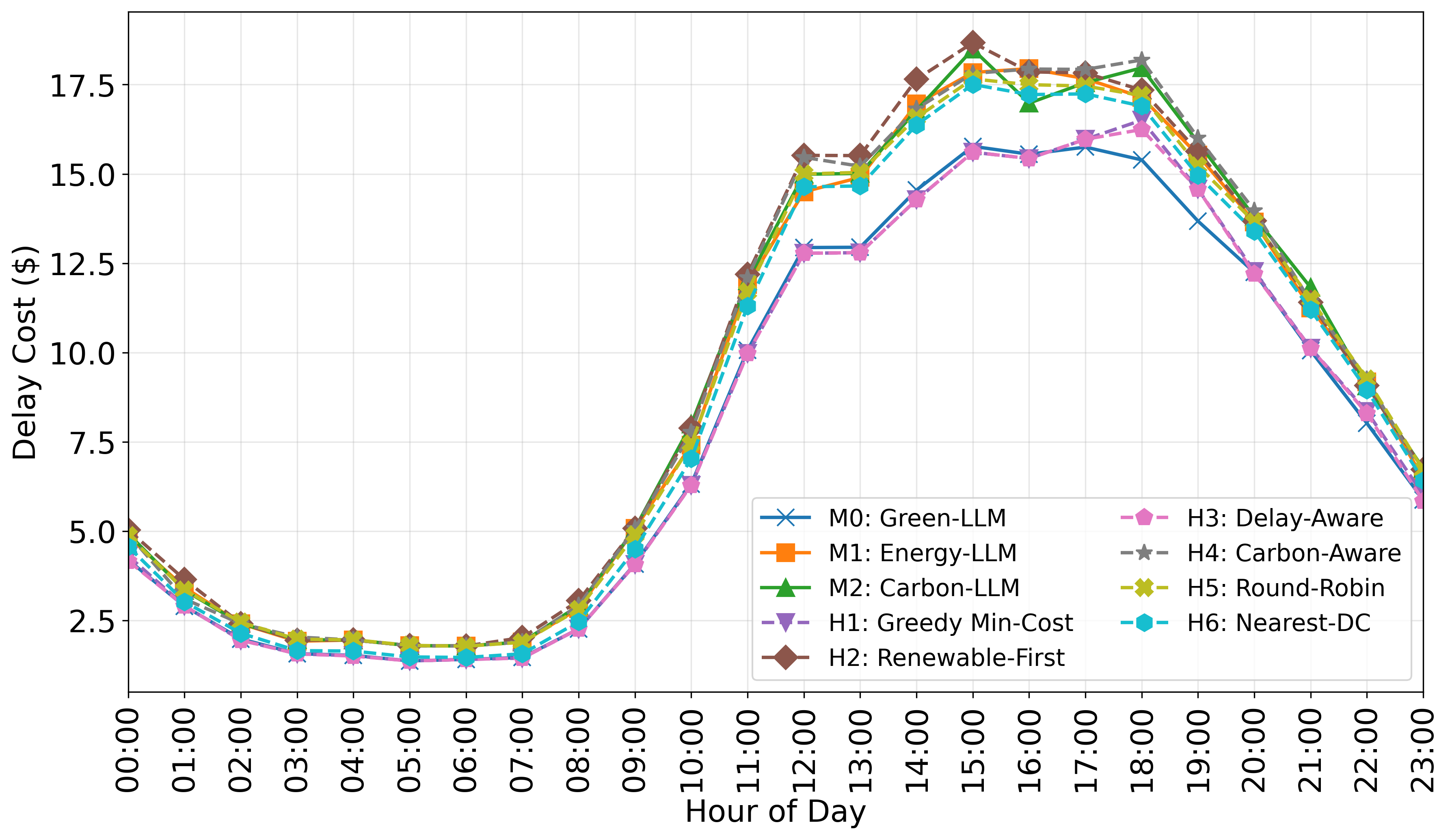
1) Varying carbon intensity: Fig. 1(a) illustrates the trade-off between carbon emission and total operational costs as the carbon intensity scaling factor $\theta$ changes across these models. A lower value of $\Psi_{\theta}$ indicates a cleaner energy mix in the power grid supplying the DCs. Overall, M0 consistently achieves the lowest cost with minimal sensitivity to carbon intensity $\theta$. Carbon-aware approaches (M2,H4) show only mild cost increases, reflecting their preference for low-carbon DCs. In contrast, energy and delay-driven heuristics (H1–H3,H5–H6) experience steep, linear cost growth as $\Psi_{\theta}$ rises. These methods fail to internalize time-varying carbon intensity and are therefore forced to avoid carbon-heavy locations reactively. Figs. 1(c)–1(d) further reveal that this divergence is driven by late afternoon and evening emission spikes, when grid carbon intensity is highest. Delay-aware heuristics are particularly affected as their reliance on geographically proximate DCs locks them into carbon-intensive regions during peak hours.

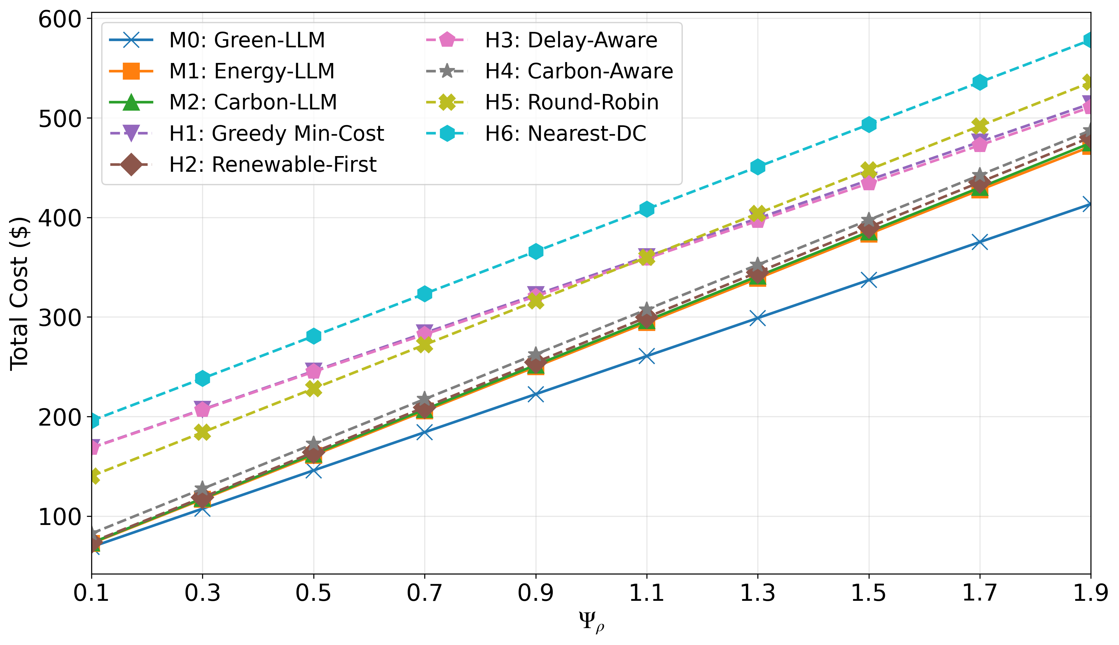
2) Varying renewable energy: Fig. 1(b) shows total cost decreases as renewable availability increases since more renewable energy becomes available, reducing reliance on the carbon-intensive grid. Figs. 1(e)–1(f) show the time series breakdown when $\Psi_{w}=0.7$, implying that renewable energy delivers the greatest marginal benefit during peak-demand periods, when both delay and carbon costs are high. Heuristic approaches, which rely on static or single-objective, fail to align renewable utilization with these high-impact periods. In contrast, M0 coordinates workload across time and locations to exploit renewable resources during peak hours, thereby suppressing both congestion and carbon peaks, achieving the lowest total cost. M1 and M2 improve over heuristics but remain suboptimal since they capture part of this benefit but lack full system-level coordination due to myopic decisions.

(a) Total cost: varying $\tau$

(b) Carbon emission: varying $\tau$

(c) Delay: varying $\rho$

(d) Total cost: varying $\rho$ and $\tau$

Figure 2: Varying token size $\mathbf{\tau}$ and delay penalty $\rho$: M0 is robust in managing inference workloads where large token sizes and delay penalties coexist.

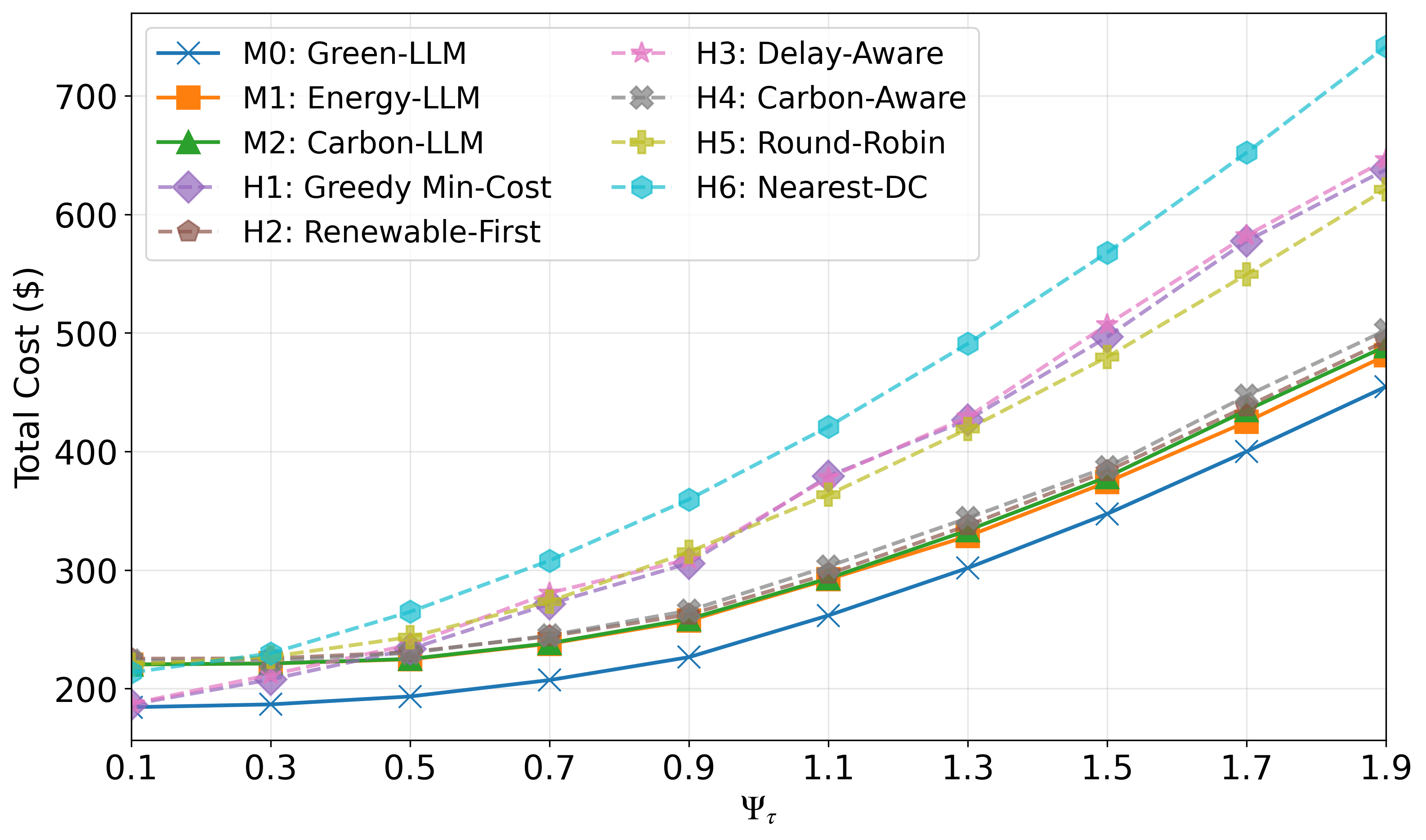
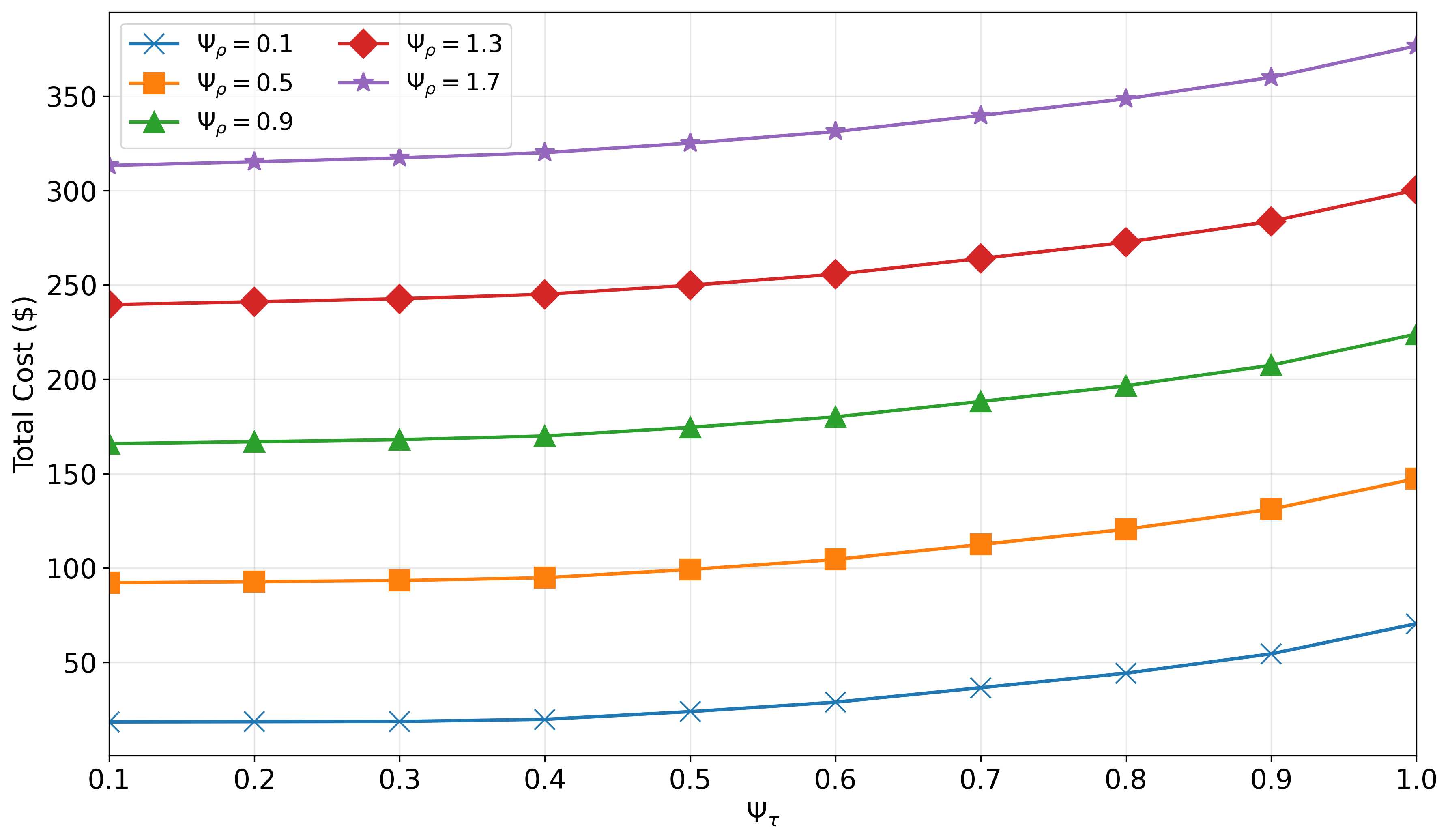
3) Impacts of other parameters: Figs. 2(a)–2(b) examine how token size $\tau$ and delay penalty $\rho$ influence system performance. As shown in Figs. 2(a)–2(b), as $\Psi_{\tau}$ increases (i.e., larger token size), the total carbon emission and total cost rise sharply for all models since a higher $\Psi_{\tau}$ corresponds to longer processing durations and increased computational load. M1 is most sensitive to token size, while M2 maintains low emissions at a higher cost. M0 achieves a favorable balance. Heuristics (H1,H3,H5,H6) exhibit the steepest growth, as they rely on fixed, single-metric rules and cannot adapt to the compounded effects of computation intensity, congestion, and energy conditions. (H2, H4) partially mitigate emissions but still suffer higher costs under large token sizes due to their myopic allocation strategies. Fig. 2(c) explores the effect of increasing delay penalties ($\Psi_{\rho}$) on total cost. As expected, higher penalty weights drive up the cost across all models. M0 remains the most cost-efficient, while heuristic approaches become increasingly unstable, particularly when large token sizes amplify delay-induced penalties.

4) Method selections: The comparative analyses of lexicographic and weighted formulations for Green-LLM are shown in Tables III-B–III-B. The results reveal that the lexicographic scheme delivers strict compliance with a chosen hierarchy of objectives but induces significant performance differences where total cost, carbon, or latency can swing by over $100\%$ when the top priority shifts. In contrast, the weighted formulation yields a smoother response by fine-tuning the weight vector. We observe that even a modest increase in the carbon weight (e.g., $\sigma_{c}=0.6$) can reduce carbon emissions by nearly half with less than a $1\%$ increase in cost. Similarly, adjusting the delay weight yields noticeable latency improvements at negligible additional expense—trade-offs that would require substantially higher cost under lexicographic delay- or carbon-first priorities. Weighted-sum models yield Pareto-efficient trade-offs across multiple objectives, whereas the lexicographic method is more appropriate when strict SLA constraints impose hard priorities on a single metric that cannot be violated.

TABLE I: Lexicographic optimization results under different priority orders (E: Energy, C: Carbon, D: Delay)

Priority Order	Total Cost	Energy cost	Carbon emission	Delay penalty
E $\succ$ D $\succ$ C	394.46	193.94	8.14	192.19
E $\succ$ C $\succ$ D	395.66	194.13	7.84	193.68
D $\succ$ E $\succ$ C	628.24	425.72	22.51	180.00
D $\succ$ C $\succ$ E	642.20	443.58	18.62	180.00
C $\succ$ E $\succ$ D	404.72	207.13	2.09	195.49
C $\succ$ D $\succ$ E	404.89	207.11	2.09	195.69

Weight Vector ($\sigma_{e},\sigma_{c},\sigma_{d}$)	Total cost	Energy cost	Carbon cost	Delay penalty
(0.33, 0.33, 0.33)	392.08	197.63	5.46	189.00
(0.60, 0.20, 0.20)	394.01	194.32	8.01	191.68
(0.20, 0.60, 0.20)	393.89	202.86	2.96	188.08
(0.20, 0.20, 0.60)	393.41	201.64	4.55	187.23
(0.45, 0.45, 0.10)	393.42	195.33	6.29	191.80
(0.45, 0.10, 0.45)	393.13	195.64	7.64	189.85

TABLE II: Weighted-sum optimization results under different weight vectors

IV Conclusion

This letter introduced Green-LLM, an optimization framework for LLM inference across heterogeneous edge DCs. The proposed framework jointly accounts for energy cost, carbon emissions, and water consumption to enable cost-efficient and sustainable operation without sacrificing service quality. Future work will explore uncertainty-aware extensions and investigate carbon credit market integration to further incentivize sustainable AI operations. Another promising direction is to jointly optimize LLM model placement and workload allocation to capture important system constraints, such as model compatibility, hardware requirements, and memory limitations.

References

- [1] A. A. Chien et al., “Reducing the carbon impact of generative AI inference (today and in 2035),” in Proc. Workshop Sustain. Comput. Sys., 2023, pp. 1–7.
- [2] P. Li, J. Yang, A. Wierman, and S. Ren, “Towards environmentally equitable AI via geographical load balancing,” in Proc. ACM e-Energy, 2024.
- [3] G. Wilkins, S. Keshav, and R. Mortier, “Offline energy-optimal LLM serving: Workload-based energy models for LLM inference on heterogeneous systems,” ACM SIGENERGY Energy Inform. Rev., vol. 4, no. 5, pp. 113–119, 2024.
- [4] J. Stojkovic et al., “DynamoLLM: Designing LLM inference clusters for performance and energy efficiency,” arXiv preprint arXiv:2408.00741, 2024.
- [5] C. Tian, X. Qin, and L. Li, “GreenLLM: Towards efficient large language model via energy-aware pruning,” in Proc. IEEE IWQoS, 2024.
- [6] A. Mudvari, Y. Jiang, and L. Tassiulas, “SplitLLM: Collaborative inference of LLMs for model placement and throughput optimization,” arXiv preprint arXiv:2410.10759, 2024.
- [7] T. Xia et al., “SkyLB: A locality-aware cross-region load balancer for LLM inference,” arXiv preprint arXiv:2505.24095, 2025.
- [8] A. K. Kakolyris et al., “SLO-aware GPU frequency scaling for energy efficient LLM inference serving,” arXiv preprint arXiv:2408.05235, 2024.
- [9] T. Wallace, B. Ombuki-Berman, and N. Ezzati-Jivan, “Optimization strategies for enhancing resource efficiency in transformers & large language models,” in Proc. ACM ICPE, 2025, pp. 105–112.
- [10] Y. He et al., “Demystifying cost-efficiency in LLM serving over heterogeneous GPUs,” arXiv preprint arXiv:2502.00722, 2025.
- [11] D. T. A. Nguyen, J. Cheng, N. Trieu, and D. T. Nguyen, “Optimal workload allocation for distributed edge clouds with renewable energy and battery storage,” in Proc. IEEE ICNC, 2024, pp. 700–705.
- [12] G.-D. Hoffmann and V. Majuntke, “Improving carbon emissions of federated large language model inference through classification of task-specificity,” 2024.
- [13] H. Wang, J. Huang, X. Lin, and H. Mohsenian-Rad, “Proactive demand response for data centers: A win-win solution,” IEEE Trans. Smart Grid, vol. 7, no. 3, pp. 1584–1596, 2016.
- [14] P. Li, J. Yang, M. A. Islam, and S. Ren, “Making AI less ‘thirsty’,” Commun. ACM, vol. 68, no. 7, pp. 54–61, 2025.
- [15] P. S. Gupta et al., “A dataset for research on water sustainability,” in Proc. ACM e-Energy, 2024, pp. 442–446.
- [16] D. Ge, C. Wang, Z. Xiong, and Y. Ye, “From an interior point to a corner point: Smart crossover,” INFORMS J. Comput., 2025.
- [17] Y. Zhao et al., “SeaLLM: Service-aware and latency-optimized resource sharing for large language model inference,” arXiv preprint arXiv:2504.15720, 2025.
- [18] J. Stojkovic et al., “Towards greener LLMs: Bringing energy-efficiency to the forefront of LLM inference,” arXiv preprint arXiv:2403.20306, 2024.
- [19] J. Cheng and D. T. Nguyen, “Green-LLM: Environmentally aware workload allocation for distributed inference – Technical report,” Arizona State Univ., Tech. Rep., 2025. [Online]. Available: https://tinyurl.com/28pd35hn
- [20] M. A. Islam, H. Mahmud, S. Ren, and X. Wang, “A carbon-aware incentive mechanism for greening colocation data centers,” IEEE Trans. Cloud Comput., vol. 8, no. 1, pp. 4–16, 2020.