Extracting Dual Analytic Geometries of Linear Transformations to Achieve Efficient Computation

Abstract

We propose a novel framework for fast integral operations by uncovering hidden geometries in the row and column structures of the underlying operators. This is accomplished through the Questionnaire algorithm, an iterative procedure that constructs adaptive hierarchical partition trees, revealing latent multiscale organizations and exposing local low-rank structures within the data. Guided by these geometries, we employ two complementary techniques: (1) The Butterfly algorithm, which exploits the learned hierarchical low-rank structure; and (2) Adaptive eGHWT, best tilings in both space and frequency using all levels of the generalized Haar–Walsh wavelet packets. These techniques enable efficient matrix factorization and multiplication. We coin our algorithms as Questionnaire Factorization and Fast Transform (QFFT). Unlike classical approaches that rely on prior knowledge of the underlying geometry, QFFT is fully data-driven and applicable to matrices arising from irregular or unknown distributions. Even when the rows and columns both appear mutually orthogonal, our framework identifies the intrinsic ordering of orthogonal vectors that reveal hidden sparsity of the kernel. We demonstrate the effectiveness of our approach on matrices associated with heterogeneous operators and families of orthogonal polynomials. The resulting compressed representations reduce storage complexity from $\mathcal{O}(N^{2})$ to $\mathcal{O}(N\log N)$, enabling fast computation and scalable implementation.

Keywords: QFFT, Iterative Geometry Learning, Kernel Factorization, Fast Transform

1 Introduction

A fundamental task in scientific computing is the evaluation of structured matrix–vector products of the form

$$u(y)=\sum_{x\in X}\mathcal{K}(y,x)f(x),$$ (1)

where $\mathcal{K}(y,x)$ is a kernel function defined in a discrete or continuous domain, and $X$ denotes the set of input points. When $\mathcal{K}(y,x)=e^{-2\pi ixy}$ and the points $x\in X$ are on a uniform grid, the Fast Fourier Transform (FFT) provides an optimal algorithm $\mathcal{O}(N\log N)$. The Nonuniform Fast Fourier Transform (NUFFT) [19] extends the FFT to handle irregular sampling by combining local interpolation with fast convolution. Beyond the classical Fourier transform, many special function transforms involving oscillatory kernels, such as the Fourier–Bessel transform and orthogonal polynomial transforms, also admit fast algorithms through variants of the FFT or NUFFT framework. Recent advances show that exploiting structural locality enables efficient computation. The Butterfly algorithm [38, 45] achieves efficient compression and Forward Transform by using complementary low-rank structures in dyadic partitions in the source and target domains. This results in a hierarchical factorization that supports both matrix compression and matrix–vector multiplication in $\mathcal{O}(N\log N)$ time. The Fast Multipole Method (FMM) [25, 9, 26] provides an optimal $\mathcal{O}(N)$ or $\mathcal{O}(NlogN)$ framework for evaluative kernels that exhibit hierarchical smoothness. By utilizing a tree-based partitioning of the computational domain and separating far-field interactions from near-field computations via low-rank expansions, FMM enables the large-scale simulation of potential fields and integral equations. In parallel, kernel matrices $\mathcal{K}(y,x)$ can be viewed as two-dimensional images in the frequency–space domain (”Phase space”). When the kernel exhibits a localized structure in both variables, characteristic of Calderón-Zygmund and Fourier Integral operators [7], wavelet packet [32, 27, 18, 12, 16, 5] combined with best-basis selection [17, 44, 31], provide adaptive ”phase space” decompositions into localized basis functions . These decompositions reveal sparsity patterns that enable efficient compression and fast matrix–vector multiplication. For operators that satisfy a mixed-Hölder condition relative to the underlying discovered interaction geometry, as seen in multiscale analysis on trees and graphs [22, 13, 3], the number of coefficients in a 2D Tree Haar basis required to achieve an approximation accuracy $\varepsilon$ is only $\mathcal{O}(1/\varepsilon)$.

However, past multiscale approaches rely on an a priori understanding of the kernel and the underlying hierarchical geometries of the source and target domains. They are inherently sensitive to the internal organization of the spatial and frequency partitions, specifically the ordering of nodes within the hierarchical structure [40]. Because perturbations in node arrangement can lead to structurally different decompositions, the resulting sparsity patterns and compression quality are highly dependent on the initial indexing. For instance, in the Butterfly algorithm, skeletonization patterns are governed by the relative positions of nodes within dyadic blocks; similarly, in wavelet packet analysis, the time-frequency tilings generated by best-basis selection are fundamentally shaped by the signal’s underlying ordering. In real-world applications, the geometry of the row and column domains is typically unknown. Even when coordinates are available, determining the optimal ordering for kernel factorization remains a significant challenge. This difficulty stems from the problem of data rearrangement: mapping a high-dimensional or manifold-based topology to a linear hierarchical structure is inherently lossy. While space-filling curves, such as Hilbert curves, are frequently used to preserve spatial locality by mapping multidimensional coordinates to a one-dimensional sequence, they remain highly sensitive to the orientation and scale of the input space. In non-Euclidean or high-dimensional settings, these mappings often fail to capture the intrinsic proximity required for effective low-rank partitioning. This issue is particularly evident in spectral contexts; for example, within the eigenspaces of spherical harmonics, there is no canonical or ”natural” ordering for eigenvectors sharing the same eigenvalue. Consequently, arbitrary node arrangements lead to structurally inconsistent decompositions, where minor perturbations in indexing or coordinate rotation can transform a compressible block into a dense one. Such instability significantly impacts the resulting sparsity patterns, the robustness of the basis, and the overall efficiency of the compression. Recent methods [33, 46] attempt to bypass geometric assumptions by constructing hierarchical partition trees using randomized projections. Although random projections preserve pairwise distances in high dimensions, they generally fail to uncover the nonlinear or multiscale geometric structures present in many operator-induced kernels [4]. For example, Fourier bases and orthogonal polynomials retain their orthogonality under random projections, but the underlying affinity structure they encode remains hidden. Instead, such a structure can be revealed through multiscale geometric organization [43, 11]. Consequently, adaptive tree constructions informed by multiscale geometry provide a more suitable foundation for efficient compression and interpretability.

To enable the learning of adaptive multiscale trees without predefined coordinates, we employ the Questionnaire algorithm [2] (see Algorithm 1, Section 3). This geometry-adaptive framework uncovers and exploits the latent multiscale organization of the kernel matrix by iteratively constructing hierarchical partition trees for both rows and columns. By defining a tree-based metric, the algorithm identifies an intrinsic geometry of the data (corresponding to a fixed point of the iterative tree building algorithm), allowing for the construction of a multiscale basis that is tailored to the operator’s structure rather than the physical coordinates of the domain. Using the learned multiscale structures, we construct a data-driven space-filling curve that aligns with the intrinsic geometry of the row and column domains. This reordering reveals two mutually coherent one-dimensional structures across the matrix, transforming it into a more regular and locally low-rank form. The resulting organization enables compact and efficient representations by applying Butterfly factorization or the extended generalized Haar-Walsh transform (eGHWT) [41] as a tool for wavelet best-basis selection to the induced adaptive multiscale structure.

Butterfly factorization is particularly effective for oscillatory kernels, enabling fast matrix-vector multiplication with $\mathcal{O}(N\log N)$ memory and computational complexity. On the other hand, eGHWT best-basis wavelet packet methods are well-suited to capture compressible structure in smooth or piecewise smooth operators. This entire pipeline, from geometric discovery to structured kernel factorization, defines our Questionnaire Factorization and Fast Transform (QFFT) algorithm. The remarkable aspect of this reordering of rows and columns of a kernel is the ability to apply one- or two-dimensional analytic tools to process functions on the data, and in particular compress the matrix as if it were an image.

By transitioning the representation into the higher dimensional space, one can leverage multi-resolution analysis to uncover the underlying low-rank structure of the kernel. Another key aspect is the implicit ”dilation” of the original matrix, viewed as a linear operator on $\mathbb{R}^{N}$, into a structured sparse matrix in a higher-dimensional space, such as $\mathbb{R}^{N\log N}$. In this lifted domain, the ”non-standard” matrix-vector multiplication can be performed in $\mathcal{O}{(NlogN)}$ operations, enabling both computational efficiency and scalability in practical applications.

The remainder of this paper is organized as follows. Section 2 provides the necessary mathematical background on the Butterfly algorithm and the eGHWT. We discuss how their performance is inherently sensitive to data geometry and partitioning, a limitation that serves as the primary motivation for our adaptive formulation. Section 3 details the foundations of the proposed geometry learning framework, including spectral graph theory, the coupled geometry learned via the Questionnaire algorithm, and our tree-based space-filling curve algorithm designed for optimal node reordering. In Section 4, we introduce the fast kernel multiplication techniques for each method and present the complete QFFT algorithm. Section 5 describes our evaluation methodology, including the hardware and software specifications used for the numerical simulations. Finally, Section 6 presents comprehensive numerical experiments that quantify the efficiency and effectiveness of the QFFT across various structured operators, followed by concluding remarks.

2 Kernel Factorization

We first define the multiscale tree structure that will be used throughout the subsequent sections.

Definition 2.1 (Multiscale Partition Tree Structure $T_{X}$).

Let $X=\{x_{i}\}_{i=1}^{N}$ be a set of sample points. A multiscale partition tree $T_{X}$ is a hierarchical decomposition of the index set $\{1,\dots,N\}$ into disjoint subsets, referred to as folders, denoted $\left\{V_{k}^{\ell}\right\}_{0\leq\ell\leq L,k\in\mathcal{C}_{k}^{\ell}}$, where $\ell=0,\dots,L$ indexes the level, $k$ indexes the folders at each level $\ell$, and $\mathcal{C}_{k}^{\ell}$ denotes the index set of the child folders of $V_{k}^{\ell}$. The root of the tree is $V_{0}^{0}=\{1,\dots,N\}$, and each folder $V_{k}^{\ell}$ at level $\ell$ is the disjoint union of its children at level $\ell+1$:

$$V_{k}^{\ell}=\bigcup_{m\in\mathcal{C}_{k}^{\ell}}V_{m}^{\ell+1}.$$ (2)

In the following, we review Butterfly and eGHWT. These methods exploit the local structure of the kernel matrix and yield efficient representations via multiscale compression.

2.1 Butterfly Factorization

The butterfly algorithm is a multiscale fast transform designed to efficiently apply dense integral operators arising in special function transforms. These operators yield kernel matrices that are globally dense but exhibit a localized low-rank structure when restricted to sub-blocks corresponding to well-separated regions in the input and output domains. A prototypical example is the oscillatory kernel $\mathcal{K}(y,x)=e^{i\gamma xy/4}$, which arises in Fourier integral operators and related transforms. The result of [30, 38] shows that the numerical rank of the associated integral operator, to a precision $\varepsilon$, is controlled by both the frequency parameter $\gamma$ and the size of the domainxrange to which the kernel is restricted. Similar results for the Fourier–Bessel integral operator are also derived in the same paper [38].

The butterfly algorithm leverages the localized low-rank structure of oscillatory kernels. Given a kernel matrix $\mathcal{K}(y,x)$ with $x\in X$, $y\in Y$, and $|X|=|Y|=N$, the algorithm begins by constructing dyadic partition trees $\mathcal{T}_{X}$ and $\mathcal{T}_{Y}$ in the output and input domains, respectively. These trees define a multilevel block structure, where each level $\ell\in\{0,1,\dots,L\}$, with $L=\log_{2}N$, corresponds to interactions between node pairs at the level $\ell$ of $\mathcal{T}_{X}$ and the level $L-\ell$ of $\mathcal{T}_{Y}$. At each level $\ell$, the algorithm applies interpolative decomposition (ID) [10, 24, 34] to approximate the sub-matrices corresponding to these block interactions. Specifically, given a matrix $A\in\mathbb{C}^{m\times n}$ whose $(r+1)$st singular value is sufficiently small, ID yields an approximation

$$A\approx BP.$$ (3)

Lemma 2.2.

(Interpolative Decompositon). Let $A\in\mathbb{R}^{m\times n}$ and $k$ be a positive integer such that $k\leq\min(m,n)$. There exists a matrix $B\in\mathbb{R}^{m\times k}$ consisting of a subset of the columns of $A$, and a matrix $P\in\mathbb{R}^{k\times n}$, such that:

1. $P$ contains a $k\times k$ identity matrix as a submatrix.

2. $\max_{i,j}|P|\leq 1$.

3. The spectral norm satisfies $\|P\|_{2}\leq\sqrt{k(n-k)+1}$.

4. The $k$-th singular value satisfies $\sigma_{k}(P)\geq 1$.

5. If $k=\min(m,n)$, then $A=BP$.

6. If $k<\min(m,n)$, the approximation error is bounded by:

   $$\|A-BP\|_{2}\leq\sqrt{k(n-k)+1}\,\sigma_{k+1}(A)$$

   where $\sigma_{k+1}(A)$ denotes the $(k+1)$-st largest singular value of $A$.

Let two adjacent blocks at level $\ell$ be approximated by interpolative decompositions as

$$B_{l}^{\ell}=B_{l}^{\ell+1}P^{\ell}_{l},\quad B_{r}^{\ell}=B_{r}^{\ell+1}P^{\ell}_{r}.$$ (4)

At level $\ell+1$, $B^{\ell+1}_{l}$ and $B^{\ell+1}_{r}$ merge to form new blocks. As illustrated in Figure 1, the upper portion of the parent block is constructed by merging the upper halves of $B_{l}^{\ell+1}$ and $B_{r}^{\ell+1}$, while the lower part merges the lower halves. The process of selecting representative rows or columns during this merge is referred to as skeletonization. This recursive divide-and-merge strategy continues until the coarsest level $L$ is reached, resulting in a multiscale hierarchical factorization of the original matrix. Assuming that each ID is performed with $\sigma_{r+1}<\varepsilon$, the final factorization enables efficient application of the matrix to a vector up to precision $\varepsilon$:

$$(\mathcal{K}f)(y_{i})=\sum_{j_{1}}B^{(L)}_{i,j_{L-1}}\sum_{j_{2}}P^{(L-1)}_{j_{L-1},j_{L-2}}\cdots\sum_{j}P^{(0)}_{j_{0},j}f(x_{j})+\mathcal{O}(\varepsilon),$$ (5)

where each interpolation matrix $P^{(\ell)}$ maps the function values at skeleton points at level $\ell$ to approximations on larger blocks at level $\ell+1$, and $B^{(L)}$ reconstructs the final output values using the skeletons at the finest scale.

The precomputation of the Butterfly factorization requires $\mathcal{O}(N^{2})$ operations due to the need to perform ID on all submatrices of the kernel. Assuming that the numerical rank $r$ of the merged blocks at each level remains comparable to that of the blocks at the previous level, the resulting factorization stores interpolation matrices and the basis block of the coarsest-level $B^{(L)}$, with total memory complexity $\mathcal{O}(rN\log N)$. As the kernel $\mathcal{K}(y,x)=e^{i\gamma xy/4}$, this rank-stability assumption typically holds for kernels when the row and column domains are similarly structured at each stage of the hierarchy. In [38, 45], the method is applied to a broad class of oscillatory and special-function kernels. Once constructed, the matrix-vector multiplication can be performed in $\mathcal{O}(N\log N)$ time. For a detailed discussion of the precomputation procedure, hierarchical compression, and fast matrix-vector application, we refer the reader to [38, 45].

Breakdown of Low-Rank Structure in Unstructured Domains.

The efficiency of the Butterfly algorithm relies on the assumption that the kernel matrix exhibits localized low-rank structure when restricted to geometrically coherent subdomains. This assumption typically holds when the input and output domains admit meaningful coordinates, such as the time–frequency grids in the Fourier transform case, so that adjacent blocks correspond to well-separated regions and maintain low numerical rank upon merging. However, in many real-world applications, such coordinate information may be unavailable or ill-defined. Without access to either geometric coordinates or explicit knowledge of the kernel function, it becomes challenging to identify an appropriate hierarchical structure or to construct partitions that preserve low-rank properties across scales.

Figure 1: Skeletonization

2.2 Walsh Wavelet Packet and Best Basis Selection

This section reviews key ideas from the work of Thiele and Villemoes [44], which introduced a fast, adaptive framework for time–frequency analysis based on Walsh tilings.

Walsh Wavelet Packets.

The Walsh system $\{W_{n}\}_{n=0}^{\infty}$ forms a complete orthonormal basis for $L^{2}[0,1)$, consisting of piecewise constant functions that take values in $\{\pm 1\}$. These functions are defined recursively by

$$W_{0}(t) =1,$$

$$W_{2n}(t) =W_{n}(2t)+(-1)^{n}W_{n}(2t-1),$$

$$W_{2n+1}(t) =W_{n}(2t)-(-1)^{n}W_{n}(2t-1),$$ (6)

for $t\in[0,1)$, where each $W_{n}$ has exactly $n$ sign changes. A tile is a dyadic rectangle of area one, parametrized by scale indices $j,j^{\prime},k,n\in\mathbb{N}\cup\{0\}$, with $k<2^{j}$. The associated time interval and sequency band are given by

$$I:=[2^{-j}k,2^{-j}(k+1)),\quad\omega:=[2^{j^{\prime}}n,2^{j^{\prime}}(n+1)).$$ (7)

When $j=j^{\prime}$, the tile $p=I\times\omega$ is considered unit-area. Let $\mathcal{P}$ be the collection of all of these unit-area dyadic rectangles. A localized Walsh function associated with tile $p\in\mathcal{P}$ is then defined as

$$w_{p}(t)=w_{j,k,n}(t):=2^{j/2}W_{n}(2^{j}t-k),$$ (8)

which is supported on $I$ and has $n$ sign changes corresponding to the ”sequency” band $\omega$.

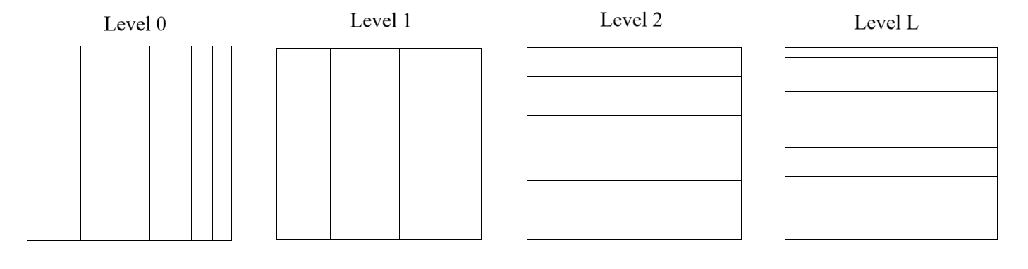
Let $N=2^{L}$ denote the signal length. A discrete signal of length $N$ can be viewed as a piecewise constant function $f\colon[0,N)\to\mathbb{R}$, where the function is constant on each unit interval $[n,n+1)$, for $n=0,1,\ldots,N-1$. The Walsh wavelet packet framework constructs an overcomplete dictionary of orthonormal functions by associating each basis atom $w_{p}$ with a dyadic space-sequency tile $p\subset\mathcal{S}_{N}:=[0,N)\times[0,1)$. At each scale $j=0,1,\ldots,L$, the domain $\mathcal{S}_{N}$ is partitioned into $N$ disjoint tiles, yielding a total of $(L+1)N$ candidate atoms. Any orthonormal basis corresponds to a disjoint partition by tiles $\mathcal{B}\subset\mathcal{P}$, where $\mathcal{P}$ denotes the full collection of tiles. The signal admits the expansion

$$f(x)=\sum_{p\in\mathcal{B}}\langle f,w_{p}\rangle w_{p}(x),$$ (9)

where orthogonality holds whenever the tiles are disjoint, i.e., $p\cap\tilde{p}=\emptyset$ for all $p\neq\tilde{p}\in\mathcal{B}$. The Walsh transform coefficients $\langle f,w_{p}\rangle$ can be computed efficiently in $O(N\log N)$ time using the Fast Walsh–Hadamard Transform (FWHT) [20], which leverages the binary structure of the basis and requires only additions and subtractions.

This construction extends naturally to two-dimensional signals. Let $\mathcal{K}\colon[0,N_{Y})\times[0,N_{X})\to\mathbb{R}$ denote an image of size $N_{Y}\times N_{X}$, where $N_{X}=2^{L}$ and $N_{Y}=2^{L^{\prime}}$. The two-dimensional Walsh wavelet packet dictionary is formed via tensor products of one-dimensional atoms:

$$w_{(p,q)}(y,x):=w_{q}(y)w_{p}(x),\quad(q,p)\in\mathcal{P}_{Y}\times\mathcal{P}_{X},$$ (10)

where each index $(q,p)$ corresponds to a dyadic tile in the product domain $\mathcal{S}_{N_{Y}}\times\mathcal{S}_{N_{X}}$. The total number of atoms in this dictionary is $(L^{\prime}+1)N_{Y}\times(L+1)N_{X}$, and any admissible two-dimensional basis corresponds to a tiling $\mathcal{B}\subset\mathcal{P}_{Y}\times\mathcal{P}_{X}$. The image may be represented as

$$\mathcal{K}(y,x)=\sum_{(q,p)\in\mathcal{B}}\langle\mathcal{K},w_{(q,p)}\rangle w_{(q,p)}(y,x),$$ (11)

with orthogonality satisfied whenever $p\cap\tilde{p}=\emptyset$ or $q\cap\tilde{q}=\emptyset$ for all $(q,p),(\tilde{q},\tilde{p})\in\mathcal{B}$.

Best Basis Selection.

Given a signal $f$ of length $N=2^{L}$, the objective of the best basis selection is to select a tiling $\mathcal{B}\subset\mathcal{P}$ such that the associated basis $\{w_{p}\}_{p\in\mathcal{B}}$ yields an efficient representation of $f$. A cost function $c(p)$ is assigned to each tile $p\in\mathcal{P}$, typically defined in terms of the magnitude of the transform coefficient $\langle f,w_{p}\rangle$. A common choice is

$$c(p):=|\langle f,w_{p}\rangle|^{\ell},$$ (12)

for $0<\ell<2$. The total cost over a tiling $\mathcal{B}$ of $\mathcal{S}_{N}$ is then given by

$$C(f,\mathcal{B}):=\sum_{p\in\mathcal{B}}c(p).$$ (13)

This cost functional is designed to be small when the energy of $f$ is concentrated in a small number of significant coefficients $\langle f,w_{p}\rangle$, making it well suited for selecting sparse or compact representations. The best basis is the tiling $\mathcal{B}^{*}=\operatorname*{arg\,min}_{\mathcal{B}}C(f,\mathcal{B})$, that minimizes the total cost $C(f,\mathcal{B})$ over all admissible tilings of $\mathcal{S}_{N}$. Thiele and Villemoes [44] proposed a dynamic programming algorithm that compares the cost of a parent tile with the combined cost of its horizontal and vertical splits, and selects the configuration with the lowest total cost. This recursive process efficiently identifies the optimal decomposition. For a signal with length $N$, the total computational complexity of the method is of $\mathcal{O}(N\log N)$.

This one-dimensional framework was later extended to two-dimensional signals, particularly in the context of image compression [31]. In the 2D setting, the analysis domain becomes $\mathcal{K}(y,x)$ on $[0,N_{X})\times[0,N_{Y})$, and adaptive tilings are constructed over dyadic rectangles in the joint space–sequency plane $\mathcal{S}_{N_{X}}\times\mathcal{S}_{N_{Y}}$. Each 2D tile corresponds to a separable product of 1D tiles. The best-basis selection algorithm applies analogously in two dimensions, recursively minimizing the total cost across hierarchical tilings. The total computational complexity is of $\mathcal{O}(N_{X}N_{Y}(\log N_{X}\log N_{Y}))$. We suggest that readers refer to [44, 31] for the technical details.

Extension to General Graph Domains.

The Generalized Haar-Walsh Transform (GHWT) [29, 41] extends the classical Haar-Walsh wavelet packet framework to signals supported on general graphs. It constructs a hierarchical dictionary of orthonormal basis vectors by recursively applying localized averaging and differencing operations over a tree-structured partition of the vertex set. Unlike classical wavelet packets, which operate on uniformly spaced dyadic intervals with an inherent linear ordering, the GHWT accommodates domains without a global coordinate system. The underlying partition tree is not restricted to binary splits; nodes may be divided into arbitrary subsets, enabling adaptive tilings that reflect the geometry of the underlying graph, while still permitting coefficient computation with $\mathcal{O}(N\log N)$ complexity, analogous to the FWHT.

The extended GHWT (eGHWT) [41] further enhances this framework by implementing a best-basis selection algorithm over the GHWT dictionary, analogous to the one- and two-dimensional best-basis algorithms developed for Haar-Walsh wavelet packets. This allows for the adaptive selection of an orthonormal basis that minimizes a user-defined cost functional, such as entropy or sparsity. The algorithm is applicable to signals of arbitrary length on graphs of general structure, without requiring $N=2^{L}$. The overall computational complexity is $\mathcal{O}(N\log N)$ for one-dimensional signals or graph-supported data under unbalanced hierarchical partitions. For two-dimensional signals, the complexity becomes $\mathcal{O}(N_{X}N_{Y}(\log N_{X}\log N_{Y}))$, analogous to the classical 2D setting. We refer the reader to [29, 41] for algorithmic details.

Ordering Ambiguity.

The construction of a hierarchical tree is central to the eGHWT, as it defines how basis vectors are recursively partitioned and labeled. However, in many cases, especially when no underlying coordinate system is available for the data domains $X$ and $Y$, the structure of the tree is not uniquely determined. This ambiguity arises not only in the choice of partition boundaries, but also in the labeling of subregions (e.g., “left” vs. “right”) at each level of the tree, which affects the binary tags assigned to basis functions. As a result, the outcome of eGHWT best-basis selection can vary, leading to different basis representations and transform coefficients for the same underlying signal and data. In [41], the tree is constructed using eigenvectors of the graph Laplacian to recursively partition the row and column domains. In the next section (see Algorithm 2, Section 3), we introduce a finer and more stable approach to tree construction in such coordinate-free settings.

3 Geometry Learning

The methods discussed above assume access to predefined tree structures. However, such hierarchies may not be available in practice. To address this limitation, we now introduce geometry-learning approaches that construct hierarchical trees directly from the data. In particular, we review techniques based on spectral graph theory and the Questionnaire algorithm, which aim to recover intrinsic affinities and multiscale structure from the underlying kernel matrix. Within this framework, we propose a data-driven space-filling curve approach to reorganize the rows and columns of the data. This reordering is designed to inherit the hierarchical tree structure while simultaneously prioritizing local smoothness. By ensuring that adjacent elements in the linear ordering share high mutual affinity, the curve creates a smooth representation that is optimal for Butterfly and eGHWT.

3.1 Spectral Graph Theory

Spectral graph theory provides a powerful framework for analyzing functions defined on graphs using the eigenstructure of matrices derived from graph connectivity. Given an undirected weighted graph $G=(V,E)$ with $N$ nodes, we define the edge weight matrix (or adjacency matrix) $W\in\mathbb{R}^{N\times N}$ such that $W_{ij}\geq 0$ encodes the affinity or similarity between nodes $i$ and $j$, with $W_{ij}=0$ if there is no edge between them. The degree matrix $D\in\mathbb{R}^{N\times N}$ is a diagonal matrix with entries $D_{ii}:=\sum_{j=1}^{N}W_{ij}$, which represents the total connection strength of node $i$ to all other nodes. From these matrices, one defines several forms of graph Laplacians, including the unnormalized Laplacian $L=D-W$, the random-walk normalized Laplacian $L_{\text{rw}}=D^{-1}L$, and the symmetric normalized Laplacian $L_{\text{sym}}=D^{-1/2}LD^{-1/2}=I-D^{-1/2}WD^{-1/2}$. When the vertices $V$ are viewed as a set of $N$ points sampled i.i.d. from a compact $m$-dimensional manifold $\mathcal{M}\subset\mathbb{R}^{d}$, the random-walk normalized Laplacian converges to the Laplace-Beltrami operator $\Delta_{\mathcal{M}}$ [42]. The unnormalized Laplacian $L$ and symmetric Laplacian $L_{\text{sym}}$ also converge to $\Delta_{\mathcal{M}}$ up to a density-dependent scaling factor [14, 37].

Lemma 3.1.

Consider a set of points $\{x_{i}\}_{i=1}^{N}$ sampled i.i.d. from a uniform distribution on a compact $d$-dimensional Riemannian manifold $\mathcal{M}\subset\mathbb{R}^{d}$. We define the affinity matrix $W\in\mathbb{R}^{N\times N}$ using a Gaussian kernel with bandwidth $\epsilon>0$:

$$W_{ij}=\exp\left(-\frac{\|x_{i}-x_{j}\|^{2}}{2\epsilon}\right).$$ (14)

Let $D$ be the diagonal degree matrix with $D_{ii}=\sum_{j}W_{ij}$. For a smooth function $f\in C^{3}(\mathcal{M})$, the discrete operator $L^{\epsilon}=L_{rw}/\epsilon$ satisfies:

$$\sum_{j=1}^{N}L^{\epsilon}_{i,j}f(x_{j})=\Delta_{\mathcal{M}}f(x_{i})+\mathcal{O}\left(\epsilon,\frac{1}{\sqrt{N}\epsilon^{d/4+1/2}}\right).$$ (15)

Under a uniform sampling distribution, the unnormalized Laplacian $L$ and symmetric Laplacian $L_{\text{sym}}$ also converge to $\Delta_{\mathcal{M}}$ up to a density-dependent scaling factor. These graph Laplacians play a central role in applications such as spectral clustering, graph signal processing, and dimensionality reduction. In particular, the random-walk Laplacian is closely related to the diffusion operator used in diffusion maps [14], a nonlinear dimensionality reduction technique that exploits the long-time behavior of random walks on graphs. Its eigenvectors form a data-driven coordinate system that preserves the geometry of the underlying data manifold. Of particular interest is the second eigenvector of $L_{\text{sym}}$, known as the Fiedler vector, which captures the most significant nontrivial mode of variation on the graph. This vector serves as a foundational tool in our framework, guiding the construction of adaptive multiscale representations through hierarchical graph partitioning.

3.1.1 Learning the Coupled Geometry by Questionnaires

In this section, we review the framework of the Questionnaire algoritm introduced in [13, 21], which provides a multiscale approach to uncover the underlying coupled geometry of a matrix by organizing its rows and columns iteratively. The key advantage of this approach is that it enables the discovery of intrinsic structures without prior knowledge of the geometry of either the row or column spaces. By identifying the most informative multiscale partitions, it projects high-dimensional rows and columns into a lower-dimensional representation that preserves the essential structural features of the original matrix. Treating the matrix entries as interactions between dual entities, the geometry is inferred directly from the data. We begin with definitions of multiscale affinities.

Definition 3.2 (Tree Affinities).

Let $X=\{x_{1},\ldots,x_{N}\}$ be a dataset, and let $\mathcal{T}_{X}=\left\{V_{k}^{\ell}\right\}_{0\leq\ell\leq L,k\in\mathcal{C}_{k}^{\ell}}$ denote a multiscale partition tree over $X$, where $V_{k}^{\ell}$ is the $k$-th folder at level $\ell$. For any function $f:X\to\mathbb{R}$, define the sample vector over folder $V_{k}^{\ell}$ as

$$f(V_{k}^{\ell}):=[f(x)]_{x\in V_{k}^{\ell}}.$$ (16)

Let the weight function $\omega:\mathcal{T}_{X}\to\mathbb{R}$ be given by

$$\omega(V_{k}^{\ell}):=2^{-\alpha\ell}\cdot|V_{k}^{\ell}|^{\beta},$$ (17)

where $\alpha\in\mathbb{R}$ controls level sensitivity, and $\beta\in\mathbb{R}$ modulates the influence of folder size.

• (Tree-based EMD): Given two functions $f,g:X\to\mathbb{R}$, the multiscale Earth Mover’s Distance over $\mathcal{T}_{X}$ is defined as

  $$EMD_{\mathcal{T}_{X}}(f,g):=\sum_{V_{k}^{\ell}\in\mathcal{T}_{X}}\left\|f(V_{k}^{\ell})-g(V_{k}^{\ell})\right\|_{1}\cdot\frac{\omega(V_{k}^{\ell})}{|V_{k}^{\ell}|}.$$ (18)

  The corresponding tree affinity is

  $$W_{\mathcal{T}_{X}}^{\mathrm{EMD}}(f,g):=\exp\left(-\frac{EMD_{\mathcal{T}_{X}}(f,g)}{\epsilon}\right),$$ (19)

  where $\epsilon>0$ is a scaling parameter.

• (Tree-based Correlation): The multiscale correlation affinity over $\mathcal{T}_{X}$ is defined as

  $$W_{\mathcal{T}_{X}}^{\mathrm{corr}}(f,g):=\sum_{V_{k}^{\ell}\in\mathcal{T}_{X}}\sum_{m\in\mathcal{C}_{k}^{\ell}}\left|\frac{\mathrm{Cov}(f(V_{m}^{\ell+1}),g(V_{m}^{\ell+1}))}{\sigma(f(V_{m}^{\ell+1}))\cdot\sigma(g(V_{m}^{\ell+1}))}\right|\frac{|V_{m}^{\ell+1}|}{|V_{k}^{\ell}|\cdot\omega(V_{m}^{\ell+1})},$$ (20)

  where $\mathrm{Cov}$ denotes the sample covariance and $\sigma$ the sample standard deviation.

Remark 3.3.

In [15], several metrics as in (18) are defined and proved equivalent to Earth Mover’s Distance with respect to the tree metric. The parameters $\alpha$, $\beta$, and $\epsilon$ modulate the effect of tree structure on the EMD. Increasing $\alpha>0$ places more weight on differences at coarser scales near the root, while $\alpha=0$ yields uniform weighting across levels and $\alpha<0$ emphasizes finer, leaf-level structure. The parameter $\beta$ controls sensitivity to folder size: $\beta>0$ favors larger folders, while $\beta<0$ emphasizes smaller ones. The parameter $\epsilon$ regulates the decay of the affinity; in practice, it is typically set as a constant multiple of the median EMD across all function pairs.

Remark 3.4.

An affinity measure between eigenfunctions was introduced in [43, 11] and is defined in the general setting of a compact Riemannian manifold as

$$W_{t}(f,g)^{2}:=\|fg\|_{L^{2}}^{-2}\int_{\mathcal{M}}\left(\int_{\mathcal{M}}p(t,x,y)(f(y)-f(x))(g(y)-g(x))\,dy\right)^{2}dx,$$ (21)

where $f$ and $g$ are eigenfunctions of an operator such as the Laplace–Beltrami operator, and $p(t,x,y)$ denotes the heat kernel with time parameter $t$. This quantity captures the local correlation of the gradients of $f$ and $g$, integrated across the manifold and smoothed by the heat kernel. A large value of $W_{t}(f,g)$ indicates that $f$ and $g$ vary coherently over the domain, whereas a small value suggests significant frequency separation or orthogonality in their local oscillation patterns. However, in many practical settings, the underlying coordinates $x$ and $y$ on the domain $\mathcal{M}$ are unknown or ill-defined, and the heat kernel $p(t,x,y)$ cannot be computed. In such cases, one cannot evaluate $W_{t}(f,g)$ directly. Instead, a multiscale data-driven approach is required. The multiscale correlation affinity $W^{\mathrm{corr}}_{\mathcal{T}_{X}}$, defined in (20), provides a surrogate by measuring normalized correlations of function averages over hierarchical partitions induced by a tree $\mathcal{T}_{X}$. While $W_{t}(f,g)$ integrates infinitesimal local interactions via diffusion, $W^{\mathrm{corr}}_{\mathcal{T}_{X}}$ captures coarse-to-fine structure based purely on observed matrix entries. Both serve as meaningful affinities between eigenfunctions or eigenvectors [11].

Now consider a kernel $\mathcal{K}:Y\times X\to\mathbb{R}$. For convenience of notation, let $W_{\mathcal{T}_{X}}$ and $W_{\mathcal{T}_{Y}}$ denote tree-based affinities on $X$ and $Y$, respectively. These affinities may be defined using either the multiscale Earth Mover’s Distance $W_{\mathcal{T}_{X}}^{\mathrm{EMD}}$, the multiscale correlation affinity $W_{\mathcal{T}_{X}}^{\mathrm{corr}}$, as introduced in Definition 3.2, or any other user-specified affinity measure constructed from the hierarchical structure of $\mathcal{T}_{X}$ or $\mathcal{T}_{Y}$.

Definition 3.5 (Coupled Geometry).

Given a partition tree $\mathcal{T}_{X}$ on $X$, the dual affinity between rows $y_{1},y_{2}\in Y$ is defined as

$$W_{\mathcal{T}_{X}}(y_{1},y_{2}):=W_{\mathcal{T}_{X}}(\mathcal{K}_{y_{1}},\mathcal{K}_{y_{2}}),$$ (22)

where each $\mathcal{K}_{y}(x):=\mathcal{K}(y,x)$ is viewed as a function on $X$.

Similarly, given a partition tree $\mathcal{T}_{Y}$ on $Y$, the dual affinity between columns $x_{1},x_{2}\in X$ is defined as

$$W_{\mathcal{T}_{Y}}(x_{1},x_{2}):=W_{\mathcal{T}_{Y}}(\mathcal{K}^{x_{1}},\mathcal{K}^{x_{2}}),$$ (23)

where $\mathcal{K}^{x}(y):=\mathcal{K}(y,x)$ is viewed as a function on $Y$.

Using these constructions, the Questionnaire algorithm [2] that iteratively refines the multiscale structures of rows and columns and the coupled geometry is constructed as the following:

Algorithm 1 Questionnaire

1:Given an initial affinity $W_{X}$ on $X$, construct a tree $\mathcal{T}_{X}$.

2:Compute the dual affinity $W_{\mathcal{T}_{X}}$ on $Y$ and build a tree $\mathcal{T}_{Y}$.

3:Compute the dual affinity $W_{\mathcal{T}_{Y}}$ on $X$ and refine $\mathcal{T}_{X}$.

4:Repeat steps 2 and 3 until either the affinities $W_{\mathcal{T}_{X}}$ and $W_{\mathcal{T}_{Y}}$ converge, or a fixed number of iterations is reached.

Remark 3.6.

In this work, at each iteration, the construction and refinement of the tree $\mathcal{T}_{X}$ (or $\mathcal{T}_{Y}$) is performed via recursive spectral bipartitioning using the Fiedler vector associated with the affinity matrix $W_{\mathcal{T}_{Y}}$ (or $W_{\mathcal{T}_{X}}$) (see Algorithm 2). This yields a hierarchical organization that reflects the intrinsic geometry of the data. While the framework allows for flexible tree constructions [2, 35], we limited our discussion here to bi-partitioning via the Fiedler vector due to its robust spectral properties and computational efficiency.

Through the iterative procedure in which the geometry of one dimension is refined based on the current organization of the other, we achieve an adaptive matrix reordering that reveals latent hierarchical patterns. These ideas were further developed in [2], which presents a practical implementation and experimental validation of the coupled geometry framework [1]. In [13, 35], they demonstrated that after such a reorganization, the resulting data-driven tree transforms yield highly sparse representations of the data. Furthermore, [3] applies wavelet shrinkage techniques and Calderón–Zygmund-type decompositions to recover structured, piecewise-smooth components from matrices exhibiting mixed Hölder regularity and provides theoretical guarantees showing that such matrices can be efficiently approximated by thresholding tensor Haar-like basis functions supported on large rectangles. [23] integrated Questionnaire algorithm to reconstruct disorganized and unlabeled datasets in chemical and bioengineering processes; by applying the framework to 1D advection–diffusion systems and ensembles of Stuart–Landau oscillators, the iterative organizational learning can reconstruct meaningful spatial and parameter embeddings from scrambled data, thereby enabling accurate data-driven identification and emulation of complex system dynamics.

3.2 Recursive Tree Construction and Spectral Space-Filling Curve

Our goal is to construct row and column trees in Algorithm 1 and their one-dimensional ordering of the domain such that the rows and columns of a data matrix reflect the intrinsic geometry of the data and support coherent multiscale representations via Butterfly algorithm and eGHWT. This can be interpreted as the construction of a space-filling curve, a continuous, surjective mapping from the unit interval onto a higher-dimensional data space, that adapts to the latent geometric structure of the data [8]. By preserving locality and conforming to the underlying patterns, such curves serve as powerful tools in a wide range of applications, including search and indexing structures, computer graphics, numerical simulation, cryptography, and the design of cache-oblivious algorithms [6]. Classical space-filling curves, such as the Hilbert [28], Peano [39], and Z-order [36] curves, provide deterministic traversals of regular Cartesian grids that approximately preserve spatial proximity. However, they rely on fixed subdivision rules and assume uniform grid structures , making them unsuitable for general data that lacks such regularity. Furthermore, these curves require a priori knowledge of the geometry and coordinate of the space, preventing them from adapting dynamically to non-uniform data density or evolving spatial extents.

We use a recursive tree construction and a space-filling curve that adapts to the intrinsic geometry of the learned tree structure and tree affinity from Algorithm 1. While standard hierarchical clustering defines the blocks of a matrix, it often neglects the continuity between them. Our approach ensures that the final linear ordering of points $\pi$ minimizes the spectral distance across every partition boundary, effectively stitching the global tree structure into a smooth 1D manifold. The final ordering is determined by identifying linkage points, indices that sit at the ”edges” of each cluster. By tracking these points through every level of the hierarchy, we orient child folders so that the exit point of one folder is always spectrally adjacent to the entrance point of its successor. This creates a continuous path where intra-cluster continuity is maintained by the local Fiedler vector ordering. Inter-cluster continuity is guaranteed by the recursive alignment of linkage points at the thresholds. The resulting permutation $\pi$ yields a reordered affinity matrix with a concentrated structure and a 1D signal representation with maximized local smoothness. See Algorithm 2 for the details.

In Figure 2, we illustrate the performance of the space-filling curve on a synthetic dataset of $2048$ points uniformly sampled on the square $[-1,1]\times[-1,1]$. The affinity matrix $W$ is computed using a Gaussian kernel based on pairwise Euclidean distances. As the level of the hierarchical partition increases, the space-filling curve progressively refines its path through the domain, revealing a smooth and coherent traversal that respects the spatial distribution of the points. At finer levels, the curve more densely fills the sampled surface, producing an ordering that captures the underlying geometry while maintaining spatial locality.

Algorithm 2 Construction of Tree and Space Filling Curve

1:Input: Affinity matrix $W\in\mathbb{R}^{N\times N}$, threshold strategy $\epsilon$ (e.g., $0$ or median).

2:Output: Tree $\mathcal{T}=\{V_{k}^{\ell}\}$ and space-filling curve $\pi$.

3:Initialize:

4:$L\leftarrow\lceil\log_{2}N\rceil$.

5:Compute $L_{\mathrm{sym}}$ for $V_{0}^{0}$ and its Fiedler vector $\mathbf{f}$.

6:Partition $V_{0}^{0}$ into $C_{<}=\{i:f_{i}<\epsilon\}$ and $C_{\geq}=\{i:f_{i}\geq\epsilon\}$.

7:$p_{<}\leftarrow\arg\max_{i\in C_{<}}f_{i}$,  $p_{\geq}\leftarrow\arg\min_{i\in C_{\geq}}f_{i}$.

8:$V_{0}^{1}\leftarrow C_{<},P_{0}^{1}\leftarrow p_{<}$;  $V_{1}^{1}\leftarrow C_{\geq},P_{1}^{1}\leftarrow p_{\geq}$.

9:

10:for level $\ell=1$ to $L-1$ do

11:  for folder $k=0$ to $2^{\ell}-1$ do

12:   Let $V=V_{k}^{\ell}$ and $P=P_{k}^{\ell}$ be the inherited linkage point.

13:   if $|V|>2$ then

14:     Compute $L_{\mathrm{sym}}$ for $W(V,V)$ and its Fiedler vector $\mathbf{f}_{V}$.

15:     Split $V$ into $C_{A},C_{B}$ using threshold $\epsilon_{V}$.

16:     $p_{A}\leftarrow\arg\max_{i\in C_{A}}f_{i}$,  $p_{B}\leftarrow\arg\min_{i\in C_{B}}f_{i}$.

17:   else$\triangleright$ Handle small folders $|V|\leq 2$ manually

18:     Let $C_{A}\leftarrow\{P\}$ and $C_{B}\leftarrow V\setminus\{P\}$.

19:     $p_{A}\leftarrow P,\quad p_{B}\leftarrow(\text{if }C_{B}\neq\emptyset\text{ then }\text{only element in }C_{B}\text{ else }\text{null})$.

20:   end if

21:   

22:   if $k$ is even then $\triangleright$ $V$ is a left sibling; $P$ is the exit to the right

23:     if $P\in C_{A}$ then

24:      $V_{2k}^{\ell+1}\leftarrow C_{B},P_{2k}^{\ell+1}\leftarrow p_{B};\quad V_{2k+1}^{\ell+1}\leftarrow C_{A},P_{2k+1}^{\ell+1}\leftarrow P$

25:     else

26:      $V_{2k}^{\ell+1}\leftarrow C_{A},P_{2k}^{\ell+1}\leftarrow p_{A};\quad V_{2k+1}^{\ell+1}\leftarrow C_{B},P_{2k+1}^{\ell+1}\leftarrow P$

27:     end if

28:   else$\triangleright$ $V$ is a right sibling; $P$ is the entrance from the left

29:     if $P\in C_{A}$ then

30:      $V_{2k}^{\ell+1}\leftarrow C_{A},P_{2k}^{\ell+1}\leftarrow P;\quad V_{2k+1}^{\ell+1}\leftarrow C_{B},P_{2k+1}^{\ell+1}\leftarrow p_{B}$

31:     else

32:      $V_{2k}^{\ell+1}\leftarrow C_{B},P_{2k}^{\ell+1}\leftarrow P;\quad V_{2k+1}^{\ell+1}\leftarrow C_{A},P_{2k+1}^{\ell+1}\leftarrow p_{A}$

33:     end if

34:   end if

35:  end for

36:end for

37:return $\mathcal{T}=\{V_{k}^{\ell}\}_{0\leq\ell\leq L,0\leq k<2^{\ell}}$ and $\pi=[V_{0}^{L},V_{1}^{L},\dots,V_{2^{L}-1}^{L}]$.

Figure 2: Visualization of the space-filling curve at each tree level. Data points are uniformly sampled from the square $[-1,1]\times[-1,1]$. Each subplot corresponds to a level of the partition tree. The title of each subplot indicates the tree level. The colors and the indices $1,2,3,\ldots$ denote the left-to-right ordering of the nodes at that level. The yellow line connects the nodes according to the space-filling curve traversal.

4 Questionnaire Factorization and Fast Transform

Based on the previous sections, our QFFT framework begins by constructing hierarchical partition trees on the rows and columns of the input matrix using Questionnaire as Algorithm 1. Based on the final dual affinities $W_{\mathcal{T}_{X}}$ and $W_{\mathcal{T}_{Y}}$, these trees are then reordered using the data-driven space-filling curve procedure described in Algorithm 2, which aligns the matrix structure with the intrinsic geometry of the data. We then apply either the Butterfly, utilizing skeletonization built from row and column partition trees, or the eGHWT to the reordered matrix to obtain a compressed representation. For the Butterfly algorithm, the compression is performed via ID maintaining a precision of given $\varepsilon$. For eGHWT, compression is achieved by retaining the largest transform coefficients such that the total approximation error remains below a user-defined threshold $\varepsilon$. In this work, we measure the approximation error using the Frobenius norm $\|\cdot\|_{F}$ and $\ell_{2}$ norm $\|\cdot\|_{\ell_{2}}$, as detailed in the following procedure. The complete process is summarized in Algorithm 3.

Algorithm 3 QFFT, Questionnaire Factorization and Fast Transform

1:Discrete matrix of kernel $\mathcal{K}\in\mathbb{R}^{N_{Y}\times N_{X}}$; error parameter $\varepsilon\in(0,1)$; initial affinity $W_{X}$; compression option: "Butterfly" or "eGHWT"

2:Apply Algorithm 1 with initial affinity $W_{X}$ to construct hierarchical partition trees $\mathcal{T}_{X},\mathcal{T}_{Y}$ and dual affinities $W_{\mathcal{T}_{X}},W_{\mathcal{T}_{Y}}$.

3:Use Algorithm 2 for tree construction; generate leaf orderings from the terminal iteration.

4:Reorganize $\mathcal{K}$ according to the final row and column leaf orderings.

5:if compression option == "Butterfly" then

6:  Apply Butterfly factorization to the reordered matrix using ID with precision $\varepsilon$.

7:  Output: Final-layer skeleton matrix $B^{(L)}$ and interpolation matrices $\{P^{(\ell)}\}$.

8:else if compression option == "eGHWT" then

9:  Apply (eGHWT) to the reorganized $\mathcal{K}$.

10:  Select best tiling $\mathcal{B}^{*}$ and best basis $\{\omega_{(q,p)}\}$ with coefficients:

11:  $c_{(q,p)}:=\langle\mathcal{K},\omega_{(q,p)}\rangle$

12:  Sort $|c_{(q,p)}|$ and retain top $n$ terms such that:

13:  $\frac{\sqrt{\sum_{i=n+1}^{N_{Y}N_{X}}c_{(q_{i},p_{i})}^{2}}}{\|\mathcal{K}\|_{F}}\leq\varepsilon$

14:  Output: Compressed coefficients $\{c_{(q_{i},p_{i})}\}_{i=1}^{n}$ and basis functions.

15:end if

We assume throughout this discussion that $N_{X},N_{Y}=O(N)$. In Algorithm 3, if the compression option Butterfly is selected, the fast kernel application is simply

$$\widehat{\mathcal{K}}f(y_{i})=\sum_{j_{1}}B^{(L)}_{i,j_{L-1}}\sum_{j_{2}}P^{(L-1)}_{j_{L-1},j_{L-2}}\cdots\sum_{j}P^{(0)}_{j_{0},j}f(x_{j}).$$ (24)

Provided that low-rank structure is successfully captured at each hierarchical level, the computational complexity of this procedure is $\mathcal{O}(N\log N)$. If the compression option eGHWT is selected, the kernel matrix $\mathcal{K}(x,y)$ is approximated using a best-basis representation

$$w_{(q_{i},p_{i})}(x,y)=w_{q_{i}}(x)w_{p_{i}}(y),$$

indexed by $(q_{i},p_{i})\in\mathcal{B}^{*}$, along with the corresponding GHWT coefficients $c_{(q_{i},p_{i})}$ for $i=1,\ldots,N_{Y}N_{X}$. To reduce storage and computational cost, only the top $n$ coefficients are retained, which sufficiently satisfy a prescribed error $\varepsilon$. Given an input vector $f\in\mathbb{R}^{N_{X}}$, interpreted as a function on the discrete domain $[0,N_{X})$, we compute its GHWT expansion coefficients:

$$c_{p}^{f}:=\langle f,w_{p}\rangle,$$

which can be obtained in $\mathcal{O}(N_{X}\log N_{X})$ time. The matrix-vector multiplication is then performed in the transform domain by aggregating over the retained basis pairs:

$$\widehat{c}_{q_{i}}:=\sum_{\begin{subarray}{c}p_{i}\text{ such that }\\ (q_{i},p_{i})\in\mathcal{B}^{*}\end{subarray}}c_{(q_{i},p_{i})}\cdot c_{p_{i}}^{f},\quad i=1,\ldots,n,$$

followed by reconstruction of the output vector via the inverse eGHWT:

$$\widehat{\mathcal{K}}f(y):=\sum_{\begin{subarray}{c}p_{i}\text{ such that }\\ (q_{i},p_{i})\in\mathcal{B}^{*}\end{subarray}}\widehat{c}_{q_{i}}\cdot w_{q_{i}}(y).$$ (25)

When $n$ is of $\mathcal{O}(N\log N)$ or smaller, the total complexity of this procedure is $\mathcal{O}(N\log N)$, offering a significant computational advantage over the $\mathcal{O}(N^{2})$ cost of direct matrix-vector multiplication.

As an illustrative example, consider the kernel of Discrete Sine Transform IV:

$$\mathcal{K}(k,x_{i})=\sin\left(\pi(k-0.5)x_{i}\right),$$ (26)

where $x_{i}=\frac{i-0.5}{N}$ (sec), $i,k=1,\ldots,N$, and $N=1024$. The discretization of the signal $y$:

$$y(x_{i})=5\sin(\pi(k_{1}+0.5)x_{i})+10\sin(\pi(k_{2}+0.5)x_{i})+5\sin(\pi(k3+0.5)x_{i})),$$ (27)

where $k_{1}=10$, $k_{2}=500$, and $k_{3}=1000$. To approximate the integral

$$\int_{0}^{1}\mathcal{K}(k,x)\,y(x)\,dx$$ (28)

by representing the kernel $\mathcal{K}$ using $O(N\log N)$ coefficients via Butterfly and the two-dimensional eGHWT. Figure 3 illustrates the result. The left panel shows the input signal $y(x_{i})$, while the right panel compares the transform results obtained using the direct multiplication of the original kernel, Butterfly with $\varepsilon=10^{-11}$, and eGHWT with $\varepsilon=5\times 10^{-2}$, demonstrating that the proposed representation accurately captures the action of the transform.

Figure 3: Approximation of the DST-IV transform using Butterfly and eGHWT. Left: the input signal $y(x)=5\sin(\pi(k_{1}+0.5)x)+10\sin(\pi(k_{2}+0.5)x)+5\sin(\pi(k3+0.5)x))$, where $k_{1}=10$, $k_{2}=500$, and $k_{3}=1000$. Right: Comparison of the transform using the direct multiplication, Butterfly with $\varepsilon=10^{-11}$, and eGHWT with $\varepsilon=5\times 10^{-2}$.

5 Evaluation

We evaluate the performance of our proposed QFFT framework on synthetic kernel matrices. Given the kernel matrices with rows and columns randomly permuted, Algorithm 1 and Algorithm 2 are employed to learn the intrinsic geometry and reorganization of the rows and columns. Once the kernel matrix has been reorganized to reveal its multiscale structure, it is compressed using Butterfly factorization and the eGHWT via Algorithm 3 under fixed precision. We report the Prep. Times of both the reorganization and compression stages, compare the memory of the original and compressed matrices, and assess the approximation accuracy and the computational efficiency of the resulting matrix-vector multiplication. All entries of the matrices are stored in Float64 format, corresponding to the standard 64-bit IEEE 754 double-precision floating-point representation. All code is implemented in Python 3. All experiments were conducted on a dual-socket system equipped with AMD EPYC 7643 processors, providing a total of 96 physical CPU cores with a base clock frequency of 2.3 GHz. The computation of the tree-based affinity in the Questionnaire algorithm was parallelized across six NVIDIA RTX A4500 GPUs, providing a total of 120 GB of GPU memory. The system used NVIDIA driver version 515.76 with CUDA 11.7 for hardware acceleration. All other algorithms, including the Butterfly and eGHWT, were executed using single CPU thread.

In the following tables, the parameter $N$ denotes the number of columns in the matrix to which our proposed algorithm is applied, while the number of rows is specified for each individual numerical example. Each table is partitioned into distinct blocks for the Butterfly, eGHWT, and Questionnaire frameworks. The “Prep. Time” row reports the computation time of each algorithm across various matrix sizes in seconds (sec). For both the Butterfly and eGHWT methods, the subsequent rows—Permuted, Original, and Reorganized—report the memory consumption in MiB after applying the factorization under different ordering schemes: a random permutation of rows and columns, the original ordering of the row and column spaces, and the matrix reorganized by our proposed QFFT method. The efficiency of the kernel application is evaluated through two metrics: “Direct Evaluation” lists the time required to perform a standard dense matrix–vector multiplication in seconds, while “Forward Transform” reports the time in seconds required to apply the factorized kernel using the accelerated algorithms described in Section 4. Finally, the “Relative $\ell_{2}$ Error” column quantifies the numerical accuracy of the application. Given a test function $f\in\mathbb{R}^{N}$ and the approximate image $\widehat{\mathcal{K}}f$, obtained via the Butterfly method (5) or the eGHWT method (25), the error is defined as

$$\frac{\|\mathcal{K}f-\widehat{\mathcal{K}}f\|_{\ell_{2}}}{\|\mathcal{K}f\|_{\ell_{2}}},$$ (29)

computed using test functions drawn uniformly at random from the interval $[0,1]$ and averaged over 300 trials. Since the best basis selection algorithm of eGHWT requires $\mathcal{O}(N^{2}(\log N)^{2})$ memory, cases where this exceeds our CPU memory capacity are indicated by “–” in the table.

6 Numerical Simulations

6.1 Eigenfunctions on $\mathbb{S}^{1}$

The functions $\sin(2\pi kx)$ and $\cos(2\pi kx)$ form the classical Fourier basis and arise as eigenfunctions of the Laplacian on the one-dimensional torus $\mathbb{S}^{1}$. In this work, we use sine functions as a representative example. To demonstrate the efficacy of the proposed approach, we ensure the discretized kernel $\mathcal{K}\in\mathbb{R}^{N\times N}$ is totally orthogonal, such that both its rows and columns form an orthogonal basis, we use the symmetric mid-point sampling scheme. Let the frequency indices be $k\in\{1,\dots,N\}$ and the spatial domain $[0,1]$ be discretized into $N$ points $x_{i}=\frac{i-0.5}{N}$ for $i=1,\dots,N$. We define the discretized kernel with entries:

$$\mathcal{K}_{ki}=\mathcal{K}(k,x_{i})=\sin\left(\pi(k-0.5)\frac{(i-0.5)}{N}\right).$$ (30)

This construction corresponds to the basis functions of the Type-IV Discrete Sine Transform (DST-IV).

Geometry learning. Denote the domains of space and frequency as $X=\{x_{i}\}_{i=1}^{N}$ and $K=\{k-0.5\}_{k=1}^{N}$. We apply Algorithm 1 to the randomly permuted domains to recover the coupled geometry of the rows and columns. The initial affinity matrix $W_{K}$ is calculated using the cosine similarity between each row. Subsequently, the multiscale tree structures $\mathcal{T}_{K}$ and $\mathcal{T}_{X}$, along with the tree-based affinities $W_{\mathcal{T}_{K}}^{\mathrm{corr}}$ and $W_{\mathcal{T}_{X}}^{\mathrm{corr}}$, are used to guide the construction of hierarchical partitions and space filling curves in Algorithm 2 for the next iteration.

Figure 4: Comparison of the initial cosine similarity matrix $W_{K}$ (top-left) and $W_{X}$ (bottom-left) with the learned multiscale correlation affinity $W_{\mathcal{T}_{X}}^{\mathrm{corr}}$(top-right) and $W_{\mathcal{T}_{K}}^{\mathrm{corr}}$ (bottom-right) among of the kernel $\sin(\pi(k-0.5)\frac{(i-0.5)}{N})$, where $X=\{x_{i}\}_{i=1}^{N}$ and $K=\{k-0.5\}_{k=1}^{N}$, for $i=1,\ldots,N$, $k=1\,\ldots,N$, and $N=256$.

As illustrated in Figure 4, the initial cosine similarity for both the frequency domain $K$ and spatial domain $X$ yields a diagonal matrix with uniform diagonal entries. Due to the orthogonality of the basis functions, these matrices capture only trivial self-similarities and fail to reveal meaningful affinity between different frequencies or sampled points. In contrast, the tree-based affinity successfully captures correlations across multiple scales, uncovering the latent structure among the frequency and space components.

We perform 10 iterations of Algorithm 1. In Figure 5(a), we display the matrix reorganized according to the row and column space-filling curves at each iteration. Remarkably, the proposed algorithm progressively uncovers the latent geometry in both the frequency and spatial domains. Even when the rows and columns of the matrix are initially orthogonal and randomly permuted, the proposed method successfully reveals the intrinsic affinities of the row and column spaces, reorganizing the matrix into a highly structured and symmetric form as the iterations proceed. Furthermore, in Figures 5(b) and (c), we present the diffusion embeddings of $W_{T_{K}}$ and $W_{T_{X}}$ at each iteration by the first three nontrivial eigenvectors of their $L_{sym}$, with the sampling points colored according to the learned space-filling curve. These diffusion embeddings reveal that the proposed algorithm gradually uncovers the underlying one-dimensional manifold structure of both the spatial domain $X$ and the frequency domain $K$. The smooth color gradients along the embeddings reflect the specific reorderings produced by Algorithm 2, illustrating how the hidden geometric relationships in both domains are progressively and successfully recovered.

(a) Reorganization.

(b) Embedding of the space $X$.

(c) Embedding of frequency space $K$.

Figure 5: Analysis of the DST-IV kernel for 10 iterations of Algorithm 1, showing (a) reorganization, (b) space embedding, and (c) frequency embedding.

Kernel Factorization. Algorithm 3 is applied to three versions of the matrix: the randomly permuted matrix, the reorganized matrix by our proposed method, and the matrix using the natural order of $k$ and $x_{i}$. For the Butterfly factorization, we initiate the skeletonization process at the finest level $\ell$ of the tree $T_{X}$ such that the maximum number of columns per block satisfies $\max_{k}|V_{k}^{\ell}|\leq 128$. The precision of each interpolative decomposition is fixed at $\varepsilon=10^{-11}$. For the factorization by eGHWT, we fix $\varepsilon=5\times 10^{-2}$. This difference in accuracy selection is because of the fact that eGHWT is constructed from simple piecewise-constant $\pm 1$ basis functions, which are not optimally suited for representing highly oscillatory kernels. Nevertheless, as we demonstrate in the following results, the matrix reorganization induced by our method still leads to a significant improvement in memory efficiency for eGHWT. In Table 1, we report the evaluation of facorization and kernel application under both Butterfly and eGHWT. For both factorization approaches, our proposed method achieves better memory efficiency on the reorganized matrix that is comparable to that of the matrix organized by the natural order ($i=1,\ldots,N$ and $k=1,\ldots,N$) and significantly outperforms the compression applied to the randomly permuted matrix. The Butterfly factorization, originally developed for oscillatory kernels, achieves high-precision approximation while maintaining both memory usage and kernel application complexity on the order of $\mathcal{O}(N\log N)$. The eGHWT factorization is based on constructing localized, data-adaptive wavelet-like basis functions over learned hierarchical trees, capturing smooth or structured patterns with reduced complexity. The Butterfly representation supports faster kernel application compared with direct multiplication, with preparation time scaling as $\mathcal{O}(N\log N)$. The eGHWT representation, while exhibiting a similar $\mathcal{O}(N\log N)$ scaling, is currently slower than direct multiplication in absolute terms due to our single-threaded implementation of the eGHWT transform. Developing an optimized fast eGHWT transform remains a direction for future work.

N 1024 2048 4096 8192 16384 32768 Direct Evaluation (sec) 5.71E-4 6.86E-3 1.66E-2 6.80E-2 3.30E-1 1.29E0 Questionnaire Prep. Time (sec) 8.90E1 1.15E2 2.76E2 1.05E3 4.47E3 1.30E4 Butterfly Permuted (MiB) 1.80E1 8.40E1 2.96E2 1.36E3 4.77E3 1.89E4 Original (MiB) 9.19E0 2.47E1 6.29E1 1.54E2 3.65E2 8.51E2 Reorganized (MiB) 6.59E0 2.06E1 6.32E1 1.50E2 4.26E2 1.45E3 Prep. Time (sec) 1.40E0 9.24E0 1.89E2 5.70E2 1.53E3 4.03E3 Forward Transform (sec) 1.05E-3 2.45E-3 8.60E-3 1.82E-2 3.71E-2 6.24E-2 Relative $\ell_{2}$ Error 9.42E-12 2.09 E-11 1.54E-11 1.45E-11 1.12E-11 1.75E-11 eGHWT Permuted (MiB) 1.43E1 5.67E1 2.25E2 8.98E2 3.59E3 – Original (MiB) 2.71E0 8.45E0 2.66E1 8.48E1 2.65E2 – Reorganized (MiB) 1.00E1 3.83E1 1.58E2 6.38E2 1.98E3 – Prep. Time (sec) 2.98E1 1.77E2 7.30E2 4.31E3 2.28E4 – Forward Transform (sec) 1.76E-1 9.69E-1 3.61E0 1.40E1 4.33E1 – Relative $\ell_{2}$ Error 3.92E-2 4.92E-2 4.92E-2 4.97E-2 4.70E-2 –

Table 1: Times, errors, and memory usage for DST-IV.

Figure 6: Comparison of computational time and memory usage for Butterfly and eGHWT in DST-IV across different sizes of $N$.

6.2 Acoustic Waves and Potential Operator

Consider an acoustic wave propagation scenario between two point clouds. We construct the row and column spaces embedded in $\mathbb{R}^{3}$: a one-dimensional helix $\{x_{i}\}_{i=1}^{N}$ (blue) and a two-dimensional sheet $\{y_{j}\}_{j=1}^{N}$ (red), as illustrated in the left panel of Figure 7. The ”acoustic” interaction between source and target points is modeled by the kernel

$$\mathcal{K}_{ij}=\frac{\cos(2\pi\nu\|x_{i}-y_{j}\|)}{\|x_{i}-y_{j}\|},$$ (31)

where $\nu$ is the frequency parameter. This kernel corresponds to the real part of the three-dimensional Helmholtz equation with wavenumber $k=2\pi\nu$. It captures oscillatory wave behavior with spatial decay and is commonly used to model time-harmonic acoustic interactions in free space as a potential operator. When $\nu=0$, the kernel simplifies to

$$\mathcal{K}_{ij}=\frac{1}{\|x_{i}-y_{j}\|},$$ (32)

which corresponds to the static Green’s function of the Laplace equation in three dimensions. In this case, the kernel models a classical potential operator describing steady-state interactions such as electrostatic or gravitational forces, with long-range influence and no oscillatory behavior. We examine the scenario with the equispaced helical source points $\{x_{i}\}$ and the non-equispaced target points $\{y_{j}\}$ on the sheet, both are randomly shuffled and remain unorganized.

Geometry Learning. We apply our proposed method to recover the intrinsic structure from the permuted kernel matrix and reorganize it accordingly, revealing the underlying geometric correspondence between the source and target domains. For Algorithm 1, the initial affinity matrix $W_{X}$ is computed using a Gaussian kernel, $W_{X}(i,j)=\exp\left(-\frac{\|x_{i}-x_{j}\|^{2}}{2\sigma^{2}}\right),$ where $\sigma=\textup{median}_{x_{i},x_{j}\in X}\|x_{i}-x_{j}\|$. The multiscale trees $\mathcal{T}_{X}$ and $\mathcal{T}_{Y}$, along with the corresponding tree-based affinities $W_{\mathcal{T}_{X}}^{\mathrm{EMD}}$ and $W_{\mathcal{T}_{Y}}^{\mathrm{EMD}}$, are used to guide the construction of hierarchical partitions and to determine the ordering via a space-filling curve in Algorithm 2. As shown in the middle and the right panel of Figure 7, which visualize the clustering structure of $\mathcal{T}_{X}$ and $\mathcal{T}_{Y}$ for the Green function and the Helmholtz kernel with $\nu=1$, respectively. Our QFFT approach effectively uncovers how the helical and planar components interact as encoded within the kernel data matrix. Rather than relying on the extrinsic physical coordinates, which may not align with the kernel’s behavior, our method reorganizes the rows and columns of the interaction matrix into a highly structured, analytical form. Figures 9 and  9 illustrate the corresponding kernel matrices before and after organization by Algorithm 1, for the potential operator and the acoustic wave. The reorganized matrices reveal pronounced local regularity and smooth, blockwise structure, highlighting the effectiveness of the learned geometry in organizing the data.

Figure 7: Left: spatial layout of the helix (points $\{x_{i}\}_{i=1}^{N}$) and the flat sheet (points $\{y_{j}\}_{j=1}^{N}$). Middle: same layout, with points colored according to tree-based space filling curve learned via Algorithm 2 for the kernel $\frac{1}{\left\lVert x_{i}-y_{j}\right\rVert}$. Right: same layout, with points colored according to tree-based space filling curve learned via Algorithm 2 for the kernel $\frac{\cos(2\pi\left\lVert x_{i}-y_{j}\right\rVert)}{\left\lVert x_{i}-y_{j}\right\rVert}$.

Figure 8: The unorganized matrix of potential operator $\frac{1}{\left\lVert x_{i}-y_{j}\right\rVert}$ (left) and after reorganizing the rows and columns (right).

Figure 9: The unorganized matrix of $\frac{\cos(2\pi\left\lVert x_{i}-y_{j}\right\rVert)}{\left\lVert x_{i}-y_{j}\right\rVert}$ (left) and after reorganizing the rows and columns (right).

Kernel Factorization For both setup, we apply Algorithm 3 to factorize the corresponding kernel. For Butterfly factorization, we start the skeletonization process at the finest level $\ell$ of the tree $T_{X}$ such that the maximum number of columns per block satisfies $\max_{k}|V_{k}^{\ell}|\leq 64$. The precision of each ID is fixed at $\varepsilon=10^{-11}$ for all values of $\nu$. For the eGHWT-based factorization, the threshold is set to $\varepsilon=10^{-4}$ for both of the potential operator and the acoustic wave kernels. In Tables 2 and 3, we report the performance of the factorizations and the corresponding kernel applications across varying sample sizes $N$. For both factorization approaches, our geometry-adaptive method achieves significantly better compression performance on the reorganized matrix compared to the unorganized input. As $N$ increases, both methods produce compressed representations with less memory usage than the randomly permuted one. The Butterfly factorization provides high-precision approximation while maintaining both memory usage and application complexity on the order of $\mathcal{O}(N\log N)$. The eGHWT factorization is particularly effective in capturing this interaction structure by utilizing localized, data-adaptive wavelet-like bases. By hierarchically partitioning the rows and columns based on the kernel’s behavior, this approach effectively organizes the interaction matrix into an $\mathcal{H}$-matrix framework. Under fixed precision, memory usage scales better than $\mathcal{O}(N\log N)$, and the kernel application remains efficient at $\mathcal{O}(N\log N)$ due to the eGHWT transform.

N 1024 2048 4096 8192 16384 32768 Direct Evaluation 7.12E-4 3.68E-3 1.78E-2 8.10E-2 3.31E-1 1.32E0 Questionnaire Prep. Time (sec) 5.58E1 9.16E1 2.28E2 1.00E3 2.51E3 1.20E4 Butterfly Permuted (MiB) 2.43E0 6.51E0 1.83E1 5.49E1 1.78E2 5.97E2 Reorganized (MiB) 1.03E0 2.98E0 9.81E0 3.54E1 1.34E2 5.23E2 Prep. Time (sec) 4.71E-1 7.35E-1 3.26E0 1.55E1 6.31E1 3.38E2 Forward Transform (sec) 3.53E-4 1.16E-3 2.60E-3 5.91E-3 1.21E-2 3.48E-2 Relative $\ell_{2}$ Error 3.81E-12 3.44 E-12 3.68E-12 4.05E-12 4.20E-12 4.23E-12 eGHWT Permuted (MiB) 1.31E1 5.12E1 2.04E2 8.18E2 3.30E3 – Reorganized (MiB) 4.72E-1 7.41E-1 1.03E0 1.38E0 1.83E0 – Prep. Time (sec) 4.45E1 2.00E2 7.63E2 4.04E3 2.27E4 – Forward Transform (sec) 1.01E-1 2.12E-1 4.44E-1 9.42E-1 1.99E0 – Relative $\ell_{2}$ Error 1.15E-4 1.22E-4 1.31E-4 1.48E-4 1.68E-4 –

Table 2: Times, errors, and memory usage for Green function $\frac{1}{\left\lVert x-y\right\rVert}$.

Figure 10: Comparison of computational time and memory usage for Butterfly and eGHWT in Green function $\frac{1}{\left\lVert x-y\right\rVert}$ across different sizes of $N$.

N 1024 2048 4096 8192 16384 32768 Direct Evaluation 9.14E-4 6.08E-3 2.56E-2 8.13E-2 3.33E-1 1.32E0 Questionnaire Prep. Time (sec) 5.61E1 8.78E1 2.74E2 1.14E3 2.67E3 1.60E4 Butterfly Permuted (MiB) 8.64E0 2.29E1 5.83E1 1.49E2 3.97E2 1.12E3 Reorganized (MiB) 3.99E0 9.93E0 2.04E1 5.60E1 1.68E2 5.74E2 Prep. Time (sec) 4.85E-1 1.55E0 4.94E0 2.22E1 7.68E1 3.01E2 Forward Transform (sec) 4.61E-4 1.96E-3 3.78E-3 8.02E-3 1.62E-2 3.79E-2 Relative $\ell_{2}$ Error 2.43E-11 2.67E-11 2.27E-11 2.71E-11 2.66E-11 2.28E-11 eGHWT Permuted (MiB) 2.22E1 8.91E1 3.56E2 1.42E3 5.70E3 – Reorganized (MiB) 1.32E1 3.81E1 9.40E1 2.19E2 4.48E2 – Prep. Time (sec) 3.18E1 1.72E2 7.38E2 3.79E3 2.27E4 – Forward Transform (sec) 3.53E-1 9.81E-1 2.36E0 5.41E0 1.14E1 – Relative $\ell_{2}$ Error 2.89E-4 2.07E-4 1.61E-4 1.37E-4 1.2E-4 –

Table 3: Times, errors, and memory usage for Helmholtz Kernel $\frac{\cos(2\pi\left\lVert x-y\right\rVert)}{\left\lVert x-y\right\rVert}$ factorized by Butterfly and eGHWT.

Figure 11: Comparison of computational time and memory usage for Butterfly and eGHWT in Helmholtz Kernel $\frac{\cos(2\pi\left\lVert x-y\right\rVert)}{\left\lVert x-y\right\rVert}$ across different sizes of $N$.

6.3 Spherical Harmonics

The goal is to factorize the eigenfunctions of the Laplace–Beltrami operator on the sphere. These eigenfunctions, denoted $Y_{l}^{m}$, form an orthonormal basis of $L^{2}(\mathbb{S}^{2})$, indexed by the degree $l\in\mathbb{N}\cup\{0\}$ and order $-l\leq m\leq l$, and satisfy the eigenvalue equation

$$\Delta_{\mathbb{S}^{2}}Y_{l}^{m}=-l(l+1)Y_{l}^{m}.$$ (33)

The eigenvalues grow quadratically in $l$, and the total number of spherical harmonics up to degree $l_{max}$ is $(l_{max}+1)^{2}$. Once the north pole is fixed, the spherical coordinate system becomes well-defined. We consider the real-valued version of the spherical harmonics, defined on a regular grid in spherical coordinates. Let $\theta\in[0,\pi]$ denote the colatitude and $\phi\in[0,2\pi)$ denote the azimuth. The real spherical harmonics are given by

$$Y_{l}^{m}(\theta,\phi)=\begin{cases}\sqrt{2}\,N_{l}^{|m|}\,P_{l}^{|m|}(\cos\theta)\cos(m\phi),&m>0,\\ N_{l}^{0}\,P_{l}^{0}(\cos\theta),&m=0,\\ \sqrt{2}\,N_{l}^{|m|}\,P_{l}^{|m|}(\cos\theta)\sin(|m|\phi),&m<0,\end{cases}$$ (34)

where $P_{l}^{m}$ are the associated Legendre polynomials and $N_{l}^{m}$ is the normalization constant $N_{l}^{m}=\sqrt{\frac{(2l+1)}{4\pi}\cdot\frac{(l-m)!}{(l+m)!}}.$

We consider two types of sampling schemes on the sphere for evaluating spherical harmonics. (1) Structured grid: Given a maximum degree $l_{\max}$, we define a regular grid with $N_{\theta}=N_{\phi}=2(l_{\max}+1)$, such that the colatitude values $\theta\in[0,\pi]$ are sampled uniformly as $\theta_{a}=\frac{(a+0.5)\pi}{N_{\theta}},\quad a=0,1,\ldots,N_{\theta}-1,$ and the azimuth values $\phi\in[0,2\pi)$ are sampled uniformly as $\phi_{b}=\frac{2\pi b}{N_{\phi}},\quad b=0,1,\ldots,N_{\phi}-1.$ In total we have $N=N_{\theta}N_{\phi}=4(l_{max}+1)^{2}$ points sampled on the sphere, which is comparable to the total number of eigenfunction sampled $(l_{max}+1)^{2}$. (2) Random sampling: Alternatively, we consider a random sampling of $N$ points uniformly on the sphere. The colatitude $\theta\in[0,\pi]$ is sampled via $\theta_{j}=\arccos(1-2x_{j})$, where $x_{j}\sim\textup{Uniform}(0,1)$, and the azimuth $\phi\in[0,2\pi)$ is sampled uniformly as $\phi_{j}\sim\textup{Uniform}(0,2\pi),$ for $j=1,\ldots,N$. The largest degree is set as $l_{max}=\lfloor-1+\sqrt{\frac{N}{4}}\rfloor$ such that in total we have near $N/4$ number of eigenvectors. The spherical harmonic is discretized into a basis matrix $\mathcal{K}\in\mathbb{R}^{\frac{N}{4}\times N}$. The row space of the basis matrix $\mathcal{K}$ is composed of discretized eigenfunctions that span the collection of eigenspaces $\bigoplus_{l=0}^{l_{\max}}\mathcal{H}_{l}$, where each $\mathcal{H}_{l}:=\mathrm{span}\{Y_{l}^{m}\}_{m=-l}^{l}$ constitutes a $(2l+1)$-dimensional subspace associated with the Laplace-Beltrami operator on the unit sphere. For both sampling schemes, the rows are organized in an order-major lexicographical sequence. In this arrangement, the eigenfunctions are grouped by their azimuthal order $m\in\{-l_{\max},\dots,l_{\max}\}$, and for each fixed $m$, the rows are ordered by increasing degree $l$ such that $|m|\leq l\leq l_{\max}$. Defining $S(n)=\frac{n(n+1)}{2}$ as the $n$-th triangular number, the row index $i\in\{0,\ldots,N/4\}$ is mapped from the azimuth order $m$ and degree $\ell$ as:

$$i(l,m)=\begin{cases}S(l_{\max}+m)+l+m&\text{if }m<0\\ S(l_{\max})+S(l_{\max}+1)-S(l_{\max}-m+1)+l-m&\text{if }m\geq 0\end{cases}$$ (35)

This formulation ensures basis functions of the same azimuthal frequency are clustered, thereby exposing the block-diagonal structure of the kernel operator under rotational symmetry. For the structured grid, the column index $j\in\{0,\dots,N-1\}$ is mapped from the discrete grid indices $(a,b)$ as:

$$j(a,b)=aN_{\phi}+b$$ (36)

where $a\in\{0,\dots,N_{\theta}-1\}$ and $b\in\{0,\dots,N_{\phi}-1\}$ denote the indices for colatitude and azimuthal angles, respectively, such that the colatitude and azimuthal point at $j$-th column is $(\theta_{a},\phi_{b})$. This arrangement corresponds to longitudinal scans at fixed latitudinal rings. For the random sampling scheme, the column ordering follows the sequence of the randomly generated points.

Geometry Learning. To discover a meaningful organization of both the eigenfunctions and the sample points on the sphere, we apply Algorithm 1 to the matrix of spherical harmonic eigenvectors. Let $K$ denote the index set of eigenfunctions, and let $X$ denote the set of sampled spatial points on the sphere. The initial affinity matrix $W_{K}$ is computed using cosine similarity. Multiscale trees $\mathcal{T}_{X}$ and $\mathcal{T}_{K}$ are constructed, and the corresponding tree-based affinities $W_{\mathcal{T}_{X}}^{\mathrm{corr}}$ and $W_{\mathcal{T}_{K}}^{\mathrm{corr}}$ are used to guide hierarchical partitioning. This is followed by Algorithm 2, which recovers an intrinsic reordering that reflects the underlying geometric structure of both domains.

Figure 12 illustrates the embeddings of the eigenvector space $K$ and the point cloud $X$ for two sampling schemes: (a) a structured grid and (b) random sampling. For each scheme, the left panel displays the embedding of $K$, derived from the first three eigenvectors of the symmetric Laplacian $L_{sym}$ (computed from $W^{corr}_{T_{X}}$ during the final iteration of Algorithm 1). The right panel shows the spatial embedding of $X$. Both embeddings are color-coded by the space-filling curves generated via Algorithm 2, which smoothly traverse the point cloud. These visualizations reveal a latent organization within both the spherical harmonic basis and the spatial domain learned directly from the data. Figure 13 displays the kernel matrices for $l_{max}=11$ ($N=484$) across both sampling schemes. The matrices are compared in three states: the original ordering, a randomly shuffled version, and the reorganized structure produced by the space-filling curve from Algorithm 2. For the structured grid, the original organization inherently possesses high local regularity. In contrast, the randomly sampled points and the randomly permuted kernels appear as noisy, irregular distributions. However, for both sampling schemes, the reorganization via the learned space-filling curves successfully recovers the inherent local regularity and block-wise structures that were previously latent in the data.

(a) Structured Grid

(b) Random Sampling

Figure 12: Embedding results for spherical harmonic eigenvectors and sampled points on the unit sphere. The color gradient is according to the learned space-filling curve ordering. Left: Diffusion embedding of the spherical harmonic eigenvectors. Right: Embedding of the sampled points on the unit sphere.

(a) Structured Grid

(b) Random Sampling

Figure 13: Matrix of spherical harmonics basis functions sampled from two different schemes. Each panel displays the transformation from the original matrix (Top), the randomly permuted matrix (Middle), to the reorganized matrix (Bottom).

Kernel Factorization. We apply Algorithm 3 to both the structured grid and random sampling configurations. For each setup, we evaluate the performance of the Butterfly and eGHWT across three versions of the kernel matrix: the original, the randomly permuted, and the reorganized version. For Butterfly, skeletonization is initiated at the finest level $\ell$ of the tree $T_{X}$ such that the maximum number of columns per block satisfies $\max_{k}|V_{k}^{\ell}|\leq 64$, with the precision for each interpolative decomposition fixed at $\varepsilon=10^{-11}$. For the eGHWT, the threshold is set to $\varepsilon=5\times 10^{-2}$. The resulting factorization performance and kernel application costs for the structured and random cases are summarized in Tables 4 and 5, respectively. In all configurations, our proposed data-driven clustering and reorganization achieve significantly better compression performance than the same factorization of the randomly permuted matrix. As $N$ increases, Butterfly consistently achieves high-precision approximation while maintaining empirical memory usage and kernel application complexity on the order of $O(N\log N)$. Due to the inherent complexity and oscillatory nature of spherical harmonics, the memory usage of the eGHWT factorization remains close to $O(N^{2})$ under fixed precision.

N 484 1024 2116 4096 8100 16384 $l_{max}$ 11 14 23 32 45 64 Direct Evaluation 1.30E-4 5.13E-4 2.23E-3 7.64E-3 3.48E-2 1.14E-1 Questionnaire Prep. Time (sec) 6.91E1 7.77E1 9.50E1 1.54E2 2.52E2 1.18E3 Butterfly Permuted (MiB) 1.04E0 5.48E0 2.52E1 8.97E1 3.10E2 1.44E3 Original (MiB) 8.75E-1 2.77E0 8.98E0 2.14E1 6.95E1 1.73E2 Reorganized (MiB) 9.31E-1 2.87E0 8.99E0 2.27E1 7.78E1 1.75E2 Prep. Time (sec) 3.91E-2 4.04E-1 3.57E0 8.19E0 3.06E1 5.77E2 Forward Transform (sec) 1.57E-4 3.83E-4 2.02E-3 3.86E-3 1.08E-2 2.92E-2 Relative $\ell_{2}$ Error 5.43E-12 7.25E-12 6.25E-12 6.19E-12 8.58E-12 1.05E-11 eGHWT Permuted (MiB) 9.70E-1 3.93E0 1.74E1 6.14E1 2.40E2 9.50E2 Original (MiB) 7.01E-1 7.83E-1 1.11E1 1.11E1 1.27E2 1.44E2 Reorganized (MiB) 4.71E-1 9.30E-1 6.12E0 9.41E0 6.62E1 1.56E2 Prep. Time (sec) 2.42E0 7.80E0 3.25E1 1.48E2 4.46E2 3.64E3 Forward Transform (sec) 2.99E-2 6.60E-2 2.51E-1 4.59E-1 1.80E0 4.16E0 Relative $\ell_{2}$ Error 4.73E-3 2.40E-3 3.92E-3 2.71E-3 3.72E-3 2.29E-3

Table 4: Times, errors, and memory usage for spherical harmonics on structured grid factorized by Butterfly and eGHWT.

Figure 14: Comparison of computational time and memory usage for Butterfly and eGHWT in spherical harmonics on structured grid across different sizes of $N$.

N 484 1024 2116 4096 8100 16384 $l_{max}$ 11 14 23 32 45 64 Direct Evaluation 1.05E-4 5.08E-4 2.23E-3 1.13E-2 3.91E-2 1.34E-1 Questionnaire Prep. Time (sec) 6.88E1 7.72E1 9.47E1 1.66E2 2.69E2 1.22E3 Butterfly Permuted (MiB) 1.04E0 5.48E0 2.52E1 8.97E1 3.11E2 1.44E3 Original (MiB) 1.04E0 5.48E0 2.52E1 8.96E1 3.10E2 1.41E3 Reorganized (MiB) 1.04E0 5.37E0 1.81E1 6.79E1 1.80E2 5.42E2 Prep. Time (sec) 8.39E-2 5.26E-1 2.09E0 1.01E1 2.53E1 5.65E2 Forward Transform (sec) 1.93E-4 1.42E-3 5.06E-3 8.09E-3 2.04E-2 4.13E-2 Relative $\ell_{2}$ Error 5.73E-12 6.51E-12 9.13E-12 1.07E-11 3.60E-11 1.95E-11 eGHWT Permuted (MiB) 1.07E0 4.73E0 2.00E1 7.39E1 2.83E2 1.15E3 Original (MiB) 1.01E0 4.37E0 1.82E1 6.54E1 2.48E2 9.71E2 Reorganized (MiB) 8.88E-1 3.77E0 1.55E1 5.67E1 2.10E2 8.30E2 Prep. Time (sec) 2.37E0 7.80E0 3.20E1 1.47E2 4.46E2 3.62E3 Forward Transform (sec) 3.99E-2 1.28E-1 4.28E-1 1.37E0 4.84E0 1.78E1 Relative $\ell_{2}$ Error 4.73E-3 4.50E-3 4.80E-3 5.00E-3 4.72E-3 4.94E-3

Table 5: Times, errors, and memory usage for spherical harmonics on randomly sampled sphere factorized by Butterfly and eGHWT.

Figure 15: Comparison of computational time and memory usage for Butterfly and eGHWT in randomly sampled spherical harmonics across different sizes of $N$.

6.4 Approximated Laplacian of Riemannian Manifold

For an arbitrary Riemannian manifold $(\mathcal{M},g)$, there is generally no derived closed-form solution for the eigenfunctions of the Laplace-Beltrami operator $\Delta_{\mathcal{M}}$. Unlike simple Euclidean domains or highly symmetric spaces, such as the $n$-sphere or flat tori, where eigenfunctions are expressed via spherical harmonics or Fourier bases, a deformed manifold structure necessitates numerical approximation via discrete differential geometry. We design a ”twisted bean” manifold $\mathcal{M}$ as a 2D surface embedded in $\mathbb{R}^{3}$, by uniformly sampling $N$ points over the parameter domain $(u,v)\in\left[-\frac{\pi}{2},\frac{\pi}{2}\right]\times[0,2\pi]$. The variables $u$ and $v$ are drawn independently from uniform distributions on their respective intervals. The geometry is defined by the mapping $\mathbf{x}(u,v)=[x,y,z]^{T}$:

$$x =L\sin u$$

$$y =r(u)\cos v\cos(tL\sin u)-\left[r(u)\sin v+0.4(L\sin u)^{2}\right]\sin(tL\sin u)$$

$$z =r(u)\cos v\sin(tL\sin u)+\left[r(u)\sin v+0.4(L\sin u)^{2}\right]\cos(tL\sin u)$$

where $r(u)=W\cos u(1-0.2\cos u)$ modulates the transverse cross-section. We set the scaling factors $L=0.8$, $W=0.4$, and the twist intensity $t=-0.05$. This results in a dataset $\mathbf{X}=\{\mathbf{x}_{i}\}_{i=1}^{N}\subset\mathbb{R}^{3}$, representing a discrete realization of a smooth, curved manifold with varying local density. Figure 16 demonstrates $N=2^{15}$ points sampled on the twisted manifold, colored according to the longitudinal parameter $u\in[-\frac{\pi}{2},\frac{\pi}{2}]$. The color gradient $(u)$ highlights the mapping to the embedded 3D coordinates, illustrating the geometric stretching and torsional twisting relative to the manifold’s primary axis.

Figure 16: Embedding of the Twisted Manifold.

To approximate the intrinsic Laplacian $\Delta_{\mathcal{M}}$, we construct a global adjacency matrix $W$ using a Gaussian kernel with a self-tuning bandwidth:

$$W_{ij}=\exp\left(-\frac{\|\mathbf{x}_{i}-\mathbf{x}_{j}\|^{2}}{\sigma_{i}\sigma_{j}}\right)$$ (37)

where $\sigma_{i}$ is determined by the distance to the $30^{th}$ percentile of the $i^{th}$ point’s $k$-nearest neighbors. To recover the true Laplace-Beltrami operator $(\Delta_{\mathcal{M}})$ regardless of the sampling density, an anisotropic normalization is applied such that $W^{(1)}=D^{-1}WD^{-1}$, where $D$ is the degree matrix. This renormalization ensures the kernel treats the manifold as if it were uniformly sampled. “‘latex We then compute the symmetric normalized Laplacian $L_{\mathrm{sym}}=I-D_{1}^{-1/2}W^{(1)}D_{1}^{-1/2}$, where $D_{1}$ is the degree matrix of $W^{(1)}$, and solve the eigenvalue problem $L_{\mathrm{sym}}\bm{\psi}=\lambda\bm{\psi}$. The resulting eigenvectors are mapped back to the random-walk basis via $\bm{\Phi}=D_{1}^{-1/2}\bm{\psi}$, yielding discretized eigenvectors of $\Delta_{\mathcal{M}}$ that capture the natural harmonics of the manifold. The basis matrix $\mathcal{K}\in\mathbb{R}^{\lfloor N/4\rfloor\times N}$ is then constructed so that its row space is spanned by the discretized eigenfunctions corresponding to the $\lfloor N/4\rfloor$ smallest eigenvalues.

Geometry Learning. Similar as the spherical harmonics, to discover a meaningful organization of both the eigenfunctions and the sample points on the twisted manifold, we apply Algorithm 1 to the matrix of discretized eigenvectors of $\Delta_{\mathcal{M}}$. Let $K$ denote the index set of eigenfunctions, and let $X$ denote the set of sampled spatial points on the $\mathcal{M}$. The initial affinity matrix $W_{K}$ is computed using cosine similarity. Multiscale trees $\mathcal{T}_{X}$ and $\mathcal{T}_{K}$ are constructed, and the corresponding tree-based affinities $W_{\mathcal{T}_{X}}^{\mathrm{corr}}$ and $W_{\mathcal{T}_{K}}^{\mathrm{corr}}$ are used to guide hierarchical partitioning. Algorithm 2 recovers an intrinsic reordering that reflects the underlying geometric structure of both domains.

Figure 17 illustrates the embeddings of the eigenvector space $K$ and the point cloud $X$. The left panel displays the embedding of $K$, derived from the first three eigenvectors of the symmetric Laplacian computed from $W^{corr}_{T_{X}}$ during the final iteration of Algorithm 1. The right panel shows the spatial embedding of $X$. Both embeddings are color-coded by the space-filling curves generated via Algorithm 2, which smoothly traverse the point cloud. These visualizations reveal a latent organization within both the Laplacian eigenvectors and the spatial domain learned directly from the data.

Figure 17: Embedding results for Laplacain eigenvectors and sampled points on the twsited manifold. The color gradient is according to the learned space-filling curve ordering. Left: Diffusion embedding of the eigenvectors. Right: Embedding of the sampled points on the twisted manifold.

Figure 18 displays the kernel matrices for $N=2048$. The randomly shuffled version and the reorganized structure produced by the space-filling curve from Algorithm 2 are compared. The randomly sampled points and the randomly permuted kernels appear as noisy, irregular distributions. The reorganization via the learned space-filling curves successfully recovers the inherent local regularity and block-wise structures in the data.

Figure 18: Matrix of Laplacain eigenvectors sampled from the twisted manifold. The left panel displays the randomly permuted matrix, and the right panel displays the reorganized matrix.

Kernel Factorization. We apply Algorithm 3 and evaluate the performance of the Butterfly and eGHWT for the randomly permuted and the reorganized version. For Butterfly, skeletonization is initiated at the finest level $\ell$ of the tree $T_{X}$ such that the maximum number of columns per block satisfies $\max_{k}|V_{k}^{\ell}|\leq 256$, with the precision for each interpolative decomposition fixed at $\varepsilon=10^{-6}$. For the eGHWT, the threshold is set to $\varepsilon=5\times 10^{-2}$. The resulting factorization performance and kernel application costs are summarized in Table 6. In all configurations, our proposed data-driven clustering and reorganization achieve significantly smaller memory usage than the same factorization of the randomly permuted matrix. As $N$ increases, Butterfly consistently achieves high-precision approximation while maintaining empirical memory usage and kernel application complexity on the order of $O(N\log N)$. Due to the inherent complexity and oscillatory nature of eigenvectors, the memory usage of the eGHWT factorization remains close to $O(N^{2})$ under fixed precision.

N 1024 2048 4096 8192 16384 32768 Direct Evaluation 1.85E-4 6.54E-4 6.81E-3 2.61E-2 9.13E-2 3.32E-1 Questionnaire Prep. Time (sec) 8.95E1 1.17E2 1.82E2 4.05E2 1.75E3 5.32E3 Butterfly Permuted (MB) 4.67E0 1.76E1 8.37E1 2.98E2 1.37E3 4.84E3 Reorganized (MB) 3.19E0 1.42E1 5.42E1 1.98E2 6.81E2 2.22E3 Prep. Time (sec) 5.19E-1 1.39E0 6.01E0 3.96E1 1.44E2 6.31E2 Forward Transform (sec) 1.56E-4 4.52E-4 1.56E-3 5.20E-3 1.61E-2 5.17E-2 Relative $\ell_{2}$ Error 2.06E-7 2.18E-7 2.07E-7 2.05E-7 1.92 E-7 1.77E-7 eGHWT Permuted (MiB) 3.43E0 1.39E1 5.53E1 2.22E2 8.86E2 – Reorganized (MiB) 2.68E0 1.12E1 4.48E1 1.80E2 7.21E2 – Prep. Time (sec) 7.72E0 3.68E1 1.44E2 7.23E2 3.86E3 – Forward Transform (sec) 1.09E-1 3.46E-1 1.18E1 4.22E1 1.57E2 – Relative $\ell_{2}$ Error 2.83E-2 2.69E-2 2.75E-2 2.76E-2 2.75E-2 –

Table 6: Times, errors, and memory usage for eigenvectors $L_{rw}$ of the twisted manifold.

Figure 19: Comparison of computational time and memory usage for Butterfly and eGHWT in eigenvectors $L_{rw}$ of the twisted manifold across different sizes of $N$.

7 Discussion and Future Work

We have presented the QFFT framework, which integrates multiscale geometry learning with hierarchical matrix factorization to achieve efficient computation without prior knowledge of the domain’s coordinate system. By employing the Questionnaire algorithm, we effectively uncover latent structures in row and column spaces, allowing the Butterfly and eGHWT algorithms to operate on an intrinsically ”smooth” representation of the data.

Our numerical experiments demonstrate that the Butterfly factorization remains highly robust for oscillatory kernels, such as those arising from spherical harmonics and Helmholtz operators, maintaining high precision with $\mathcal{O}(N\log N)$ complexity. While the eGHWT approach provides significant memory compression for structured and piecewise-smooth operators, its current implementation for the forward transform is limited by single-threaded execution. Future work will focus on the parallelization and algorithmic optimization of the eGHWT transform to make it competitive with direct evaluations at larger scales.

A critical component of this framework is the iterative refinement process within the Questionnaire algorithm. While we have shown empirical success across diverse geometries, the formal theoretical analysis of the convergence criteria and the stability of the fixed points in the dual-tree construction remain open questions. We will explore these mathematical foundations in an upcoming paper. Finally, we intend to extend the QFFT framework to higher-dimensional tensor decompositions and more complex kernels arising in non-Euclidean machine learning applications.

Code Availability

The source code for the proposed method, including the QFFT and examples for eigenfunctions on $\mathbb{S}^{1}$, Green’s functions, Helmholtz kernels, spherical harmonics, and Laplacian kernels, is available at https://github.com/pei-chun-su/QuestionnaireFastTransform.jl.

References

- [1] Pyquest github repository. Note: https://github.com/hgfalling/pyquestAccessed: 2025-04-04 Cited by: §3.1.1.
- [2] (2014) Geometry and analysis of dual networks on questionnaires. Yale University. Cited by: §1, §3.1.1, §3.1.1, Remark 3.6.
- [3] (2018) Mixed hölder matrix discovery via wavelet shrinkage and calderón–zygmund decompositions. Applied and Computational Harmonic Analysis 45 (3), pp. 551–596. Cited by: §1, §3.1.1.
- [4] (2003) Laplacian eigenmaps for dimensionality reduction and data representation. Neural computation 15 (6), pp. 1373–1396. Cited by: §1.
- [5] (1991) Fast wavelet transforms and numerical algorithms i. Communications on pure and applied mathematics 44 (2), pp. 141–183. Cited by: §1.
- [6] (2020) Space-filling curves for high-performance data mining. arXiv preprint arXiv:2008.01684. Cited by: §3.2.
- [7] (1952) On the existence of certain singular integrals. In Selected Papers of Antoni Zygmund, pp. 19–73. Cited by: §1.
- [8] (1878) Ein beitrag zur mannigfaltigkeitslehre. Journal für die reine und angewandte Mathematik (Crelles Journal) 1878 (84), pp. 242–258. Cited by: §3.2.
- [9] (1988) A fast adaptive multipole algorithm for particle simulations. SIAM journal on scientific and statistical computing 9 (4), pp. 669–686. Cited by: §1.
- [10] (2005) On the compression of low rank matrices. SIAM Journal on Scientific Computing 26 (4), pp. 1389–1404. Cited by: §2.1.
- [11] (2021) On the dual geometry of laplacian eigenfunctions. Experimental Mathematics 30 (2), pp. 283–293. Cited by: §1, Remark 3.4, Remark 3.4.
- [12] (1992) Biorthogonal bases of compactly supported wavelets. Communications on pure and applied mathematics 45 (5), pp. 485–560. Cited by: §1.
- [13] (2011) Harmonic analysis of digital data bases. Wavelets and Multiscale Analysis: Theory and Applications, pp. 161–197. Cited by: §1, §3.1.1, §3.1.1.
- [14] (2006) Diffusion maps. Applied and computational harmonic analysis 21 (1), pp. 5–30. Cited by: §3.1, §3.1.
- [15] (2013) Earth mover’s distance and equivalent metrics for spaces with hierarchical partition trees. Yale CS Techinical Report. Cited by: Remark 3.3.
- [16] (1994) Signal processing and compression with wavelet packets. In Wavelets and their applications, pp. 363–379. Cited by: §1.
- [17] (1992) Entropy-based algorithms for best basis selection. IEEE Transactions on information theory 38 (2), pp. 713–718. Cited by: §1.
- [18] (1992) Ten lectures on wavelets. SIAM. Cited by: §1.
- [19] (1993) Fast fourier transforms for nonequispaced data. SIAM Journal on Scientific computing 14 (6), pp. 1368–1393. Cited by: §1.
- [20] (1976) Unified matrix treatment of the fast walsh-hadamard transform. IEEE Transactions on Computers 100 (11), pp. 1142–1146. Cited by: §2.2.
- [21] (2012) Sampling, denoising and compression of matrices by coherent matrix organization. Applied and Computational Harmonic Analysis 33 (3), pp. 354–369. Cited by: §3.1.1.
- [22] (2010) Multiscale wavelets on trees, graphs and high dimensional data: theory and applications to semi supervised learning.. In Icml, Vol. 10, pp. 367–74. Cited by: §1.
- [23] (2025) From clutter to clarity: emergent neural operators via questionnaire metrics. Computers & Chemical Engineering, pp. 109201. Cited by: §3.1.1.
- [24] (2001) The maximal-volume concept in approximation by low-rank matrices. Contemporary Mathematics 280, pp. 47–52. Cited by: §2.1.
- [25] (1987) A fast algorithm for particle simulations. Journal of computational physics 73 (2), pp. 325–348. Cited by: §1.
- [26] (1997) A new version of the fast multipole method for the laplace equation in three dimensions. Acta numerica 6, pp. 229–269. Cited by: §1.
- [27] (2012) Wavelets, approximation, and statistical applications. Vol. 129, Springer Science & Business Media. Cited by: §1.
- [28] (1935) Über die stetige abbildung einer linie auf ein flächenstück. Dritter Band: Analysis· Grundlagen der Mathematik· Physik Verschiedenes: Nebst Einer Lebensgeschichte, pp. 1–2. Cited by: §3.2.
- [29] (2015) Applied and computational harmonic analysis on graphs and networks. In Wavelets and Sparsity XVI, Vol. 9597, pp. 336–350. Cited by: §2.2, §2.2.
- [30] (1962) Prolate spheroidal wave functions, fourier analysis and uncertainty—iii: the dimension of the space of essentially time-and band-limited signals. Bell System Technical Journal 41 (4), pp. 1295–1336. Cited by: §2.1.
- [31] (2000) Image compression with adaptive haar-walsh tilings. In Wavelet Applications in Signal and Image Processing VIII, Vol. 4119, pp. 911–921. Cited by: §1, §2.2.
- [32] (1999) A wavelet tour of signal processing. Elsevier. Cited by: §1.
- [33] (2016) ASKIT: an efficient, parallel library for high-dimensional kernel summations. SIAM Journal on Scientific Computing 38 (5), pp. S720–S749. Cited by: §1.
- [34] (2007) On interpolation and integration in finite-dimensional spaces of bounded functions. Communications in Applied Mathematics and Computational Science 1 (1), pp. 133–142. Cited by: §2.1.
- [35] (2017) Data-driven tree transforms and metrics. IEEE transactions on signal and information processing over networks 4 (3), pp. 451–466. Cited by: §3.1.1, Remark 3.6.
- [36] (1966) A computer oriented geodetic data base and a new technique in file sequencing. Cited by: §3.2.
- [37] (2005) Diffusion maps, spectral clustering and eigenfunctions of fokker-planck operators. Advances in neural information processing systems 18. Cited by: §3.1.
- [38] (2010) An algorithm for the rapid evaluation of special function transforms. Applied and Computational Harmonic Analysis 28 (2), pp. 203–226. Cited by: §1, §2.1, §2.1.
- [39] (1990) Sur une courbe, qui remplit toute une aire plane. Springer. Cited by: §3.2.
- [40] (2012) Redundant wavelets on graphs and high dimensional data clouds. IEEE Signal Processing Letters 19 (5), pp. 291–294. Cited by: §1.
- [41] (2022) eGHWT: the extended generalized Haar-Walsh transform. J. Math. Imaging Vis. 64 (3), pp. 261–283. External Links: Link Cited by: §1, §2.2, §2.2, §2.2.
- [42] (2006) From graph to manifold laplacian: the convergence rate. Applied and Computational Harmonic Analysis 21 (1), pp. 128–134. Cited by: §3.1.
- [43] (2019) On the spectral resolution of products of laplacian eigenfunctions. Journal of Spectral Theory 9 (4), pp. 1367–1384. Cited by: §1, Remark 3.4.
- [44] (1996) A fast algorithm for adapted time–frequency tilings. Applied and Computational Harmonic Analysis 3 (2), pp. 91–99. Cited by: §1, §2.2, §2.2, §2.2.
- [45] (2010) Fast algorithms for spherical harmonic expansions, iii. Journal of Computational Physics 229 (18), pp. 6181–6192. Cited by: §1, §2.1.
- [46] (2017) Geometry-oblivious fmm for compressing dense spd matrices. In Proceedings of the International Conference for High Performance Computing, Networking, Storage and Analysis, pp. 1–14. Cited by: §1.