Abstract

In many settings in science and industry, such as drug discovery and clinical trials, a central challenge is designing experiments under time and budget constraints. Bayesian Optimal Experimental Design (BOED) is a paradigm to pick maximally informative designs that has been increasingly applied to such problems. During training, BOED selects inputs according to a pre-determined acquisition criterion to target informativeness. During testing, the model learned during training encounters a naturally occurring distribution of test samples. This leads to an instance of covariate shift, where the train and test samples are drawn from different distributions (the training samples are not representative of the test distribution). Prior work has shown that in the presence of model misspecification, covariate shift amplifies generalization error. Our first contribution is to provide a mathematical analysis of generalization error that reveals key contributors to generalization error in the presence of model misspecification. We show that generalization error under misspecification is the result of, in addition to covariate shift, a phenomenon we term error (de-)amplification which has not been identified or studied in prior work. We then develop a new acquisition function that mitigates the effects of model misspecification by including terms for representativeness, informativeness, and de-amplification (R-IDeA). Our experimental results demonstrate that the proposed method performs better than methods that target either only informativeness, representativeness, or both.

1 INTRODUCTION

Bayesian modeling is a principled approach to making inferences when data is scarce or costly. Most Bayesian machine learning methods are developed under the assumption that the true data-generating process (DGP) is included in the chosen model family Bernardo and Smith (2009). However, in complex real-world environments, this assumption rarely holds: The true DGP often lies outside of the assumed model family Uppal and Wang (2003); Sloman et al. (2024).This inevitability of the phenomenon of model misspecification Walker (2013) is captured by the saying that “all models are wrong” Box. (1976); Box (1980). Common causes of model misspecification include omitted variables Wooldridge (2010), mistaken beliefs about the structure of the error term (e.g., a failure to account for heteroskedasticity or autocorrelation) Greene (2003); Grünwald and Van Ommen (2017), or the choice of a misinformed or underexpressive model class Wooldridge (2010); Dubova et al. (2025). The consequences of model misspecification range from biased inferences Greene (2003); Müller (2013); Caprio et al. (2023); Bonhomme and Weidner (2022), unreliable approximations (e.g., in simulation-based inference methods Frazier et al. (2020); Lintusaari et al. (2017); Huang et al. (2023)), to suboptimal decision-making Sutton et al. (1998); Rainforth et al. (2024).

There is a substantial literature on the effects of model misspecification on Bayesian inference when data is independently and identically distributed (i.i.d.), or “passively” collected from the distribution to which the learner wants their inferences to generalize Kleijn and van der Vaart (2006, 2012); Knoblauch et al. (2022); Walker (2013); Nott et al. (2023); Kelly et al. (2025). However, in part because of the widespread availability of large datasets, active learning methods have become much more prevalent Settles (2009). These methods select the training data to tailor it to a specified learning objective Silberman (1996); Farquhar et al. (2021). Active learning methods rely on the specified model twice: once to make inferences to fit training data, and again to select the data Konyushkova et al. (2017). Model misspecification thus has a double impact on these methods, introducing potential bias in both the acquisition function and the resulting inferences. In particular, in the context of active learning, model misspecification can produce poor quality datasets Sugiyama (2005); Bach (2006); Ali et al. (2014); Vincent and Rainforth (2017); Farquhar et al. (2021). Understanding the consequences of model misspecification is of paramount importance to developing robust active learning methods.

In a Bayesian setting, Bayesian Optimal Experimental Design (BOED) is a natural and frequently used active learning method Rainforth et al. (2024); Huan et al. (2024). BOED selects the optimal design by maximizing an acquisition function known as the expected information gain, enabling budget and time efficiency Rainforth et al. (2024); Chaloner and Verdinelli (1995) in many applications, such as drug discovery Park et al. (2013), clinical trial design Chaloner and Verdinelli (1995), chemistry Walker and Ravisankar (2019); Hickman et al. (2022), biology Kreutz and Timmer (2009); Thompson et al. (2023), and psychology Cavagnaro et al. (2010); Myung et al. (2013). While the limitations of BOED in the presence of model misspecification have been acknowledged in the literature, only a limited number of papers have investigated this limitation Rainforth et al. (2024); Foster et al. (2021); Sloman et al. (2022); Schmitt et al. (2023); Ivanova et al. (2024); Barlas et al. (2025).

We provide a novel theoretical analysis of generalization error in the presence of model misspecification. Our analysis reveals that training datasets that lead to robustness to model misspecification have two properties: They are representative of the target data-generating distribution, and they are de-amplifying. The expected information gain does not include a term for either of these, and standard BOED can lead to training datasets that have neither of these characteristics. In this sense, standard BOED is not robust to model misspecification.

Unrepresentative Training Data. BOED selects samples to achieve a particular objective, and these samples likely do not reflect the distribution to which the learner would like to generalize. In other words, BOED induces a form of distribution shift, whereby the distribution used for (active) learning is different than the distribution used for evaluation. Recent work on the interaction between model misspecification and distribution shift has introduced the concept of misspecification amplification Amortila et al. (2024), whereby the generalization error attributable to misspecification is “amplified” by the density ratio between the test and training input distributions. A similar phenomenon has been observed in the context of BOED: In the presence of model misspecification, the generalization error in some settings has been shown to depend on the degree of model misspecification and the extent of distribution shift Sloman et al. (2022).

De-amplifying Training Data. As our novel decomposition of generalization error shows, generalization performance depends on not only the representativeness of the training data, but also on the way it interacts with model (mis)specification (which will be defined in Section 3): Generalization performance is enhanced when training data is in regions where the direction of model misspecification coincides with the direction in which the model would optimally learn. We refer to this property as error “de-amplification” to stress that the effect is to counteract, rather than amplify, the effect of the misspecification.

Contributions. In this work, we explore the problem of BOED under model misspecification and make the following contributions:

• Theoretical Decomposition of Generalization Error. Prior work has primarily explored the effects of misspecification and distribution shift, overlooking the role of de-amplifying designs. We formally decompose generalization error into three components: (1) misspecification bias, (2) estimation bias, and (3) a novel term we introduce, error (de-)amplification. We also derive an upper bound on generalization error that characterizes its dependence on the representativeness of the training data, the degree to which these data are de-amplifying, and model misspecification.

• Novel Acquisition Function Incorporating Representativeness and De-amplification. We propose a novel acquisition function designed to mitigate the effects of model misspecification by identifying designs that not only are informative, but are additionally representative and de-amplifying. Our empirical results show that the new acquisition outperforms traditional BOED in the presence of misspecification.

2 PRELIMINARIES

2.1 Problem Setting

General Formulation

A modeler aims to predict an observed variable $y\in\mathbb{R}^{m}$ which depends on a fully observable input (design) $\xi\in\Xi\subseteq\mathbb{R}^{d}$. The relationship between the observed variable $y$ and the input $\xi$ is governed by a conditional distribution $y|\xi\sim P^{\star}$, referred to as the true data-generating process (DGP), which depends on the output of a true (possibly unknown) regression function $f^{\star}(\xi)$ and observation noise. To approximate the true DGP, the modeler proposes a hypothetical model $f(\xi,\theta)~:~\Xi\mapsto\mathbb{R}$, where $\theta\in\Theta$ represents the parameters within the fixed parameter space $\Theta$. The model class is denoted $\mathcal{F}(\xi,\Theta)=\{f(\xi,\theta):\theta\in\Theta\}$. Model misspecification arises when the assumed model class $\mathcal{F}(\xi,\Theta)$ fails to capture the true DGP Ivanova et al. (2024); Sloman et al. (2022).

Definition 1 (Model misspecification).

Model misspecification occurs when the assumed model class $\mathcal{F}(\xi,\Theta)=\{f(\xi,\theta):\theta\in\Theta\}$ cannot mimic the true output $f^{\star}(\xi)$ for any parameter $\theta\in\Theta$. That is, the model is misspecified if

$$f^{\star}(\xi)\notin\mathcal{F}(\xi,\Theta).$$ (1)

In Bayesian inference, the modeler additionally specifies a prior distribution over the model parameters. According to this prior, the probability the data the learner will encounter is generated by a value $\theta$ is $p(\theta)$. Model fitting is carried out by updating the prior distribution using Bayes’ rule. The result is a posterior distribution which assigns to a $\theta$ a probability $p(\theta\mid y,\xi)\propto p(\theta)p(y\mid\theta,\xi)$. This process depends on both the assumed prior and the specified likelihood model. When the model is misspecified, i.e., the likelihood does not reflect the true DGP, the updated posterior becomes unreliable or biased Frazier et al. (2023); Oberauer and Musfeld .

2.2 Bayesian Optimal Experimental Design

Bayesian Optimal Experimental Design (BOED) is a model-based framework to select the optimal design $\xi$ by maximizing the expected information gained about the parameter $\theta$, enabling budget and time efficiency Rainforth et al. (2024); Chaloner and Verdinelli (1995). And the expected information gain (EIG) is expressed as below Dong et al. (2024); Lindley (1956):

$$\operatorname{EIG}(\xi) =\mathbb{E}_{p(y\mid\xi)}[\operatorname{IG}_{\theta}(\xi,y))]$$ (2)

$$=\mathbb{E}_{p(\theta,y\mid\xi)}[\log p(y\mid\theta,\xi)-\log p(y\mid\xi)]$$

The optimal design $\xi^{\star}$ is the design in a set of candidate designs $\Xi$ that maximizes the EIG:

$$\xi^{\star}={\operatorname{argmax}_{\xi\in\Xi}}\operatorname{EIG}(\xi).$$ (3)

Traditional BOED methods Foster et al. (2019); Sebastiani and Wynn (1997), also called Bayesian Adaptive Design (BAD), iterate between making design decisions by evaluating Equation 3, and updating the underlying model through Bayesian inference to condition on data obtained so far. Traditional BOED is computationally expensive, due to the substantial costs required to estimate and optimize $\operatorname{EIG}(\xi)$ and update the model at each step.

2.3 Distribution Shift

Distribution shift is a well-known challenge in machine learning. It refers to the setting where the input (design) distribution differs between the training and test phases. In BOED, training designs are selected via an acquisition criterion, while the model’s performance at test-time is evaluated on a given test distribution of interest. This mismatch induces a specific form of distribution shift known as covariate shift, where the distribution of inputs shifts (i.e., $p_{\text{train}}(\xi)\neq p_{\text{test}}(\xi)$) while the conditional output distribution remains unchanged (i.e., $p(y\mid\xi_{\text{train}})=p(y\mid\xi_{\text{test}})$). Prior work has studied the covariate shift induced by BOED Sugiyama (2005); Ali et al. (2014); Sloman et al. (2022). To address the potential resultant biases, density ratio estimation — whereby the training data are reweighted according to the estimated ratio between test and training input distributions — has proven effective Ge et al. (2023).

3 THEORETICAL RESULTS

3.1 Decomposition of Generalization Error

Recent work has demonstrated that generalization error depends on an interaction between the degree of covariate shift (the degree to which the training data are unrepresentative of the test distribution) and of model misspecification Amortila et al. (2024); Ge et al. (2023); Wen et al. (2014). In this section, we show that generalization error additionally depends on the degree of presence of a phenomenon we term error (de-)amplification. We show that generalization error can be decomposed into three terms, reflecting separate contributions of the degree of misspecification bias, of estimation bias, and of error (de-)amplification.

While prior work Hastie (2009); Sugiyama (2005) decomposed the generalization error mainly in linear regression—where the error (de-)amplification term vanishes under the orthogonality assumption between model bias and estimation error, we extend the analysis to general (nonlinear) models under misspecification, where this orthogonality no longer holds.

Notation

Let $\{(\xi_{i},y_{i})\}_{i=1}^{n}$ be a dataset of $n$ i.i.d. samples drawn from the true DGP $P^{\star}$. Denote by $f^{\star}(\xi)$ the true data-generating function. Let $\mathcal{F}$ denote the model class, and let $\hat{f}^{(n)}(\xi)$ be a learned predictor, depending on training data $\{\xi_{1},\ldots{},\xi_{n}\}$. Let $\bar{f}\in\mathcal{F}$ be the predictor that best approximates the true data-generating function $f^{\star}$, i.e., $\bar{f}=\arg\min_{f\in\mathcal{F}}R_{\mathrm{test}}(f)$.

Definition 2 (Generalization error ($R_{\mathrm{test}})$).

Let $d_{\text{test}}$ be the test data distribution. The generalization error is defined as

$$R_{\mathrm{test}}(\hat{f}^{(n)}):=\mathbb{E}_{\xi\sim d_{\text{test}}}\left[(\hat{f}^{(n)}(\xi)-f^{\star}(\xi))^{2}\right].$$ (4)

Proposition 1 (Generalization Error Decomposition).

Equation 4 can be decomposed into the following

$$R_{\mathrm{test}}(\hat{f}^{(n)}) =\underbrace{\mathbb{E}_{\xi\sim d_{\text{test}}}\left[(\bar{f}(\xi)-f^{\star}(\xi))^{2}\right]}_{\text{Misspecification Bias ($\mathbb{B}$)}}$$ (5)

$$+\underbrace{\mathbb{E}_{\xi\sim d_{\text{test}}}\left[(\hat{f}^{(n)}(\xi)-\bar{f}(\xi))^{2}\right]}_{\text{Estimation Bias ($\mathbb{C}$)}}$$

$$+\underbrace{2\,\mathbb{E}_{\xi\sim d_{\text{test}}}\left[(\bar{f}(\xi)-f^{\star}(\xi))(\hat{f}^{(n)}(\xi)-\bar{f}(\xi))\right]}_{\text{Error (de-)amplification ($\mathbb{A}$)}}.$$

In the well-specified case where the true function lies within the model class, $\bar{f}(\xi)=f^{\star}(\xi)$. In this case, both the bias and interaction terms vanish, and the generalization error reduces to:

$$R_{\mathrm{test}}(\hat{f}^{(n)})=\mathbb{E}_{\xi\sim d_{\text{test}}}\left[(\hat{f}^{(n)}(\xi)-\bar{f}(\xi))^{2}\right],$$ (6)

where the only quantity that depends on the training sample is $\hat{f}^{(n)}(\xi)$, since the test data distribution $d_{\text{test}}$ and the best predictor $\bar{f}$ are fixed.

In the misspecified case where the true function lies outside the model class, $\bar{f}(\xi)\neq f^{\star}(\xi)$. In this case, all three terms in Equation 5 contribute to generalization error. The terms have the following interpretations:

• Misspecification Bias ($\mathbb{B}$) captures the discrepancy between the best predictor and the true data-generating function, and reflects the degree of model misspecification. This term is fixed and unaffected by the training data.

• Estimation Bias ($\mathbb{C}$) captures the discrepancy between the best predictor $\bar{f}\in\mathcal{F}$ and the predictor arrived at on the basis of finite training data. In the BOED setting, this training data depends on the modeler’s sequential evaluations of the EIG.

• Error (De-)amplification ($\mathbb{A}$) measures the correlation between the extent and direction of the model’s bias and the extent and direction of the estimation error over the test distribution. This term can either amplify or mitigate the overall generalization error:

  • A positive correlation indicates that the directions of misspecification and estimation bias tend to coincide, which amplifies (increases) the generalization error.

  • A negative correlation indicates that the directions of misspecification and estimation bias tend to counteract each other, which de-amplifies (decreases) the generalization error.

3.2 An Upper Bound on Generalization Error with Error (De-)amplification

While Proposition 1 provides valuable insights into the various contributors to generalization error, computing these terms requires evaluating the outputs of $f^{\star}$ and $\bar{f}$ in expectation over the test samples. Of course, this is infeasible in practice.

To understand and control generalization error during training, the learner requires a formulation that explicitly relates it to quantities available during training. Theorem 1 provides such a formulation. Theorem 1 shows that the learner can control generalization error by selecting designs that (i) are representative of the test distribution (reduce the degree of covariate shift), and (ii) are de-amplifying (have the potential to counteract the misspecification bias). We apply these insights in our development of a novel acquisition function in Section 4.

Theorem 1 builds on a result from Amortila et al. (2024). In particular, we tighten the upper bound introduced by Amortila et al. (2024) to depend on the degree of (de-)amplification of the training samples. Their analysis requires the following definitions:

Definition 3 (The degree of covariate shift).

We assume that $d_{\text{train}}(\xi)>0$ for all $\xi\in\Xi$ and the density ratio between the test and training input distributions is Amortila et al. (2024); Sugiyama et al. (2007):

$$\mathbb{C}_{\infty}:=\sup_{\xi\in{\Xi}}|\frac{d_{\text{test}}(\xi)}{d_{\text{train}}(\xi)}|$$ (7)

where $d_{\text{train}}$ and $d_{\text{test}}$ are the training and test data distribution, respectively.

The degree of covariate shift $\mathbb{C}_{\infty}$ measures the worst-case distance between the selected training samples and the test samples. A more representative design (i.e., one that reduces covariate shift) helps control estimation bias.

Definition 4 (The degree of misspecification).

We define that the discrepancy between the predictive distribution induced by $\bar{f}$ and that of the true data-generating function $f^{\star}$ is Amortila et al. (2024):

$$\mathbb{B}_{\infty}:=\|\bar{f}-f^{\star}\|_{\infty}=\sup_{\xi\in\Xi}\mid\bar{f}(\xi)-f^{\star}(\xi)\mid$$ (8)

where $\mathbb{B}_{\infty}\geq 0$.

The degree of misspecification $\mathbb{B}_{\infty}$ measures the worst-case discrepancy between the DGP and the best predictor in the model class. In other words, it is an upper bound on the misspecification bias $\mathbb{B}$. Notice that if $\mathbb{B}_{\infty}=0$, the model is well-specified, i.e., $f^{\star}\in\mathcal{F}$. On the other hand, if $\mathbb{B}_{\infty}>0$, the model is misspecified (i.e., $f^{\star}\notin\mathcal{F}$) and $\mathbb{B}_{\infty}$ quantifies the degree of misspecification.

Assumption 1 (Boundedness of model class and outcomes Amortila et al. (2024)).

For all $\xi\in\Xi$,

$$\sup_{f\in\mathcal{F}}\|f\|_{\infty}\leq y_{\infty}\text{, }\|f^{\star}\|_{\infty}\leq y_{\infty}\text{, and }|y|\leq y_{\infty}$$

for some $y_{\infty}>0$ and where $\|f\|_{\infty}=\sup_{\xi\in\Xi}\mid f(\xi)\mid$.

Our Result.

Theorem 1 extends the result of Amortila et al. (2024) by explicitly characterizing the behavior of generalization error in a way that accounts for error (de-)amplification. While Theorem 1 characterizes generalization performance given a data set (i.e., in the data-fitting phase), it can also inform data selection by revealing properties of those data that facilitate generalization. The insights from Theorem 1 motivate us to incorporate error (de-)amplification and representativeness into the decision-making (design selection) phase, thereby reducing the generalization error in the data-fitting phase, particularly in settings with a limited number of training samples.

Theorem 1 (Generalization Error Bound under Covariate Shift with Amplification).

Let $\mathcal{F}$ be a finite model class, and let $f^{\star}$ denote the true regression function. Let $\hat{f}^{(n)}$ be the empirical risk minimizer over training data drawn from the distribution $d_{\mathrm{train}}$. Then, with probability at least $1-\delta$, the generalization error under covariate shift satisfies:

$$R_{\text{test}}(\hat{f}^{(n)})\leq\mathbb{C}_{\infty}\cdot\left\{\begin{aligned} &\mathbb{B}_{\infty}^{2}+\frac{224y_{\infty}^{2}\log(|\mathcal{F}|/\delta)}{3n}-2\widehat{\mathbb{A}}(\hat{f}^{(n)}),\\ &~\hfill\text{if }\widehat{\mathbb{A}}(\hat{f}^{(n)})<0\\ &\mathbb{B}_{\infty}^{2}+\frac{128y_{\infty}^{2}\log(|\mathcal{F}|/\delta)}{3n}-\sqrt{3}\widehat{\mathbb{A}}(\hat{f}^{(n)}),\\ &~\hfill\text{if }0\leq\widehat{\mathbb{A}}(\hat{f}^{(n)})\end{aligned}\right.$$ (9)

where $\mathbb{C}_{\infty}:=\sup_{\xi\in\Xi}\left|\frac{d_{\text{test}}(\xi)}{d_{\text{train}}(\xi)}\right|$ and $\widehat{\mathbb{A}}(\hat{f}^{(n)})\coloneqq\mathbb{E}_{\xi\sim d_{\text{train}}}\left[(\hat{f}^{(n)}(\xi)-\bar{f}(\xi))(\bar{f}(\xi)-f^{\star}(\xi))\right]$. The proof can be found in Appendix B.

Remark 1 (Connection to Proposition 1).

This bound is consistent with the full generalization error decomposition structure, including the cross-term $\widehat{\mathbb{A}}(f)$, which captures the interaction between properties of the model (misspecification bias) and of the sampling strategy (estimation bias). Proposition 1 does not explicitly reveal how the representativeness and (de-)amplifying properties of the training data interact with model bias. In contrast, Theorem 1 makes this interaction explicit, providing a more interpretable perspective for understanding and controlling the generalization error during the training phase.

Remark 2.

Proposition 1 defines the generalization error as a function of the learned function $\hat{f}^{(n)}$ and the true data-generating function $f^{\star}$, in expectation over the test distribution. However, since the true data-generating function $f^{\star}$ is unknown and outside the model class, it cannot easily offer guidance for decision-making. In contrast, although the $\widehat{\mathbb{A}}$ term that appears in Theorem 1 depends on the unknown $\bar{f}$, $\bar{f}$ is within the model class $\mathcal{F}$, which suggests that it can be better approximated in practice. We leverage this in our construction of a novel acquisition function in Section 4.2.

Remark 3.

Theorem 1 requires the assumption that $\hat{f}^{(n)}$ is the member of $\mathcal{F}$ that minimizes risk in the training data. Although our experiments adopt the Bayesian learning framework, Theorem 1 still provides valuable insights about the role of representative and (de-)amplifying training samples.

Theorem 1 reveals that the following factors contribute to generalization error:

• Representativeness of The Training Data ($\mathbb{C}_{\infty}$). The multiplicative factor of $\mathbb{C}_{\infty}$ implies that, by reducing $\mathbb{C}_{\infty}$, choosing more representative training data can reduce generalization error.

• Misspecification Bias ($\mathbb{B}_{\infty}$). Misspecification bias cannot be reduced by the training data. However, because of the multiplicative effect of $\mathbb{C}_{\infty}$, the effect of model misspecification on generalization error can be amplified by unrepresentative training samples Amortila et al. (2024).

• Error (de-)amplification ($\widehat{\mathbb{A}}$). This term captures a key component of generalization error: the interaction between the learner’s misspecification and estimation errors. The term $\widehat{\mathbb{A}}(\hat{f}^{(n)})$ can be interpreted as an average, across the training samples, of the (signed) estimation errors weighted by the (signed) misspecification errors. When $\widehat{\mathbb{A}}(\hat{f}^{(n)})$ is large (error de-amplification), the learner’s misspecification and estimation biases tend to agree, resulting in de-amplifying behavior.

  For any $\xi\in\Xi$, the misspecification error $\bar{f}(\xi)-f^{\star}(\xi)$ is fixed and cannot be removed by additional data. The objective is to induce a negative correlation between the estimation error $\hat{f}(\xi)-\bar{f}(\xi)$ and the misspecification error in regions where the misspecification error is large. In other words, when the misspecification error is large, the estimation error should not exacerbate it; ideally, the estimation error offsets (de-amplifies) the misspecification. The overall prediction error could become smaller if the de-amplifying design is selected.

  

  Figure 1: Illustration of error amplification and de-amplification. The green curve denotes the true data-generating function $f^{\star}(\xi)$, the red line represents the best-in-class approximation $\bar{f}(\xi)$, and the blue line shows the learned predictor $\hat{f}^{(n)}(\xi)$. The grey dashed shading highlights de-amplifying regions, where $\bar{f}(\xi)$ lies between $f^{\star}(\xi)$ and $\hat{f}^{(n)}(\xi)$, so that estimation error and misspecification error partially offset each other. In contrast, the remaining regions indicate amplifying regions, where estimation error reinforces misspecification, leading to larger overall prediction error.

4 TWO NOVEL ACQUISITION FUNCTIONS

Leveraging the insights from Theorem 1, we design two novel acquisition functions. R-I identifies designs that are both representative and informative about the parameter of interest. R-IDeA identifies designs that are informative, representative, and de-amplifying.

4.1 R-I: A Representative and Informative Acquisition Function

To account for covariate shift, we modify the standard EIG acquisition function by introducing a maximum mean discrepancy (MMD)-based correction term. The idea is to encourage the selection of design points that not only have high information gain but also help reduce the difference between the distributions of training and test points. Specifically, we use the following form:

$$\text{R-I}(\xi_{t})=\text{EIG}(\xi_{t})\cdot\underbrace{\left(1-\lambda\frac{\text{MMD}(h_{t-1}\cup\{\xi_{t}\},d_{\text{test}})}{\text{MMD}(h_{t-1},d_{\text{test}})}\right))}_{\text{Robust Ratio}}$$ (10)

where $h_{t-1}$ is the history of selected designs before time step $t$. The motivation and expression for MMD can be found in Appendix D.

This robust acquisition function penalizes designs that are only representative or only informative; in other words, the designs selected by R-I are both representative and informative. The hyperparameter $\lambda$ controls the tradeoff between informativeness and representativeness. When $\lambda$ tends to zero, the selected designs are informative, and R-I selects similar designs to traditional BOED.

4.2 R-IDeA: A Representative, Informative, and De-amplifying Acquisition Function

Theorem 1 shows that larger $\widehat{\mathbb{A}}(\hat{f}^{(n)})$ implies that designs on which $\hat{f}^{(n)}$ was trained de-amplify generalization error. We refer to a design $\xi$ as de-amplifying whenever $(\hat{f}^{(n)}(\xi)-\bar{f}(\xi))(\bar{f}(\xi)-f^{\star}(\xi))\geq\tau_{0}$ for a given threshold $\tau_{0}$. Ideally, we would design an acquisition function that selects only designs in the de-amplifying region $\Xi_{\mathbb{A}+}(\tau_{0})\coloneqq\Big\{\xi\in\Xi:(\hat{f}^{(n)}(\xi)-\bar{f}(\xi))(\bar{f}(\xi)-f^{\star}(\xi))\geq\tau_{0}\Big\}$. However, as discussed in Remark 2, this cannot be determined exactly since $f^{\star}$ and $\bar{f}$ are unknown. We instead construct a subset of the de-amplifying region, the approximate de-amplifying region:

Theorem 2 (Approximate de-amplifying region).

Let $\bar{f}$ be the predictor that best approximates the true data-generating function $f^{\star}$. Then,

$$\widehat{\Xi}_{\mathbb{A}+}(\tau_{1})\subseteq\Xi_{\mathbb{A}+}(\tau_{0})$$

where the approximate de-amplifying region $\widehat{\Xi}_{\mathbb{A}+}(\tau)\coloneqq\Big\{\xi\in\Xi:|\hat{f}^{(n)}(\xi)-\bar{f}(\xi)|\geq\tau_{1}\Big\}$, $\tau_{1}=\tau_{0}/\mathbb{B}_{\infty}+c\mathbb{B}_{\infty}$, $c\geq 2$, and $\tau_{0}\geq 0$. A detailed derivation can be found in Appendix C.

$\tau_{0}$ and $c$ are constants that determine the minimum threshold required for a design to be considered part of the approximate de-amplifying region.

Unlike $\Xi_{\mathbb{A}+}$, $\widehat{\Xi}_{\mathbb{A}+}$ does not depend on $f^{\star}$. However, it does depend on $\bar{f}$. As discussed in Remark 2, $\bar{f}$ is within the model class $\mathcal{F}$. Below, we leverage this in construction of the proxy approximate de-amplification region defined with a trainable proxy $g$ in Lemma 1: $\widehat{\Xi}_{\mathbb{A}+}^{g}(\tau)\coloneqq\{\xi\in\Xi:|\hat{f}^{(n)}(\xi)-g(\xi)|\geq\tau\}$.

Lemma 1 (Proxy approximate de-amplification region $\widehat{\Xi}_{\mathbb{A}+}(\tau)$).

Given a proxy function $g~:~\Xi\mapsto\mathbb{R}$ such that $\sup_{\xi\in\Xi}|g(\xi)-\bar{f}(\xi)|\leq\tau_{2}$ for some $\tau_{2}\geq 0$,

$$\widehat{\Xi}_{\mathbb{A}+}^{g}(\tau)\coloneqq\big\{\xi\in\Xi:\,|\hat{f}^{(n)}(\xi)-g(\xi)|\geq\tau\big\}\;\subseteq\;\widehat{\Xi}_{\mathbb{A}+}(\tau_{1}).$$

where $\tau=\tau_{1}+\tau_{2}$. The proof can be found in Appendix C.

Heuristically, a good proxy function $g$ (i) is aligned with $\bar{f}$, and (ii) maintains a disagreement from $\hat{f}^{(n)}$ thereby constructing a proxy de-amplifying region in Equation 12 (notice that in the extreme case where $g=\hat{f}^{(n)}$, $\widehat{\Xi}_{\mathbb{A}+}^{g}$ is empty). At time step $t$, $g$ is trained to (i) fit the observations collected up until the previous time step $\{y_{i}:i\in\{1\ldots{}t-1\}\}$, and (ii) ensure the proxy approximate de-amplification region has sufficient coverage. This leads to the following objective:

$$g=\arg\min_{g}\mathcal{L}(g) \coloneqq\frac{1}{n}\sum_{i=1}^{n}(g(\xi_{i})-y_{i})^{2}$$ (11)

$$+\frac{1}{n}\sum_{i=1}^{n}\max\!\big(0,\;\tau-|\hat{f}^{(n)}(\xi_{i})-g(\xi_{i})|\big)$$

Leveraging the proxy approximate de-amplifying region and learned $g$, we introduce an acquisition function for the decision-making phase that balances de-amplification with informativeness and representativeness. The novel acquisition function is given by

$$\text{R-IDeA{}}(\xi_{t})=\text{R-I{}}(\xi_{t})\,\mathrm{DeA}(\xi_{t}),$$ (12)

$$\text{where}\quad\mathrm{DeA}(\xi_{t})=\text{Sigmoid }\!\left(\dfrac{|\hat{f}^{(n)}(\xi_{t})-g(\xi_{t})|-\tau}{\kappa}\right),$$

where $\tau$ is as defined in Theorem 2 and further details of $\mathrm{DeA}$ are provided in Appendix C. R-IDeA requires two hyperparameters: $\tau$ corresponds to the de-amplifying threshold, i.e., to the minimum separation level required for a design to be considered in the proxy de-amplifying region, and $\kappa$ corresponds to the optional smoothing parameter. The hyperparameter $\tau$ controls the tradeoff between de-amplification and the requirements of informativeness and representativeness: When $\tau$ is large, the proxy approximate de-amplifying region is conservative in the sense that it includes only designs with very high $\widehat{\mathbb{A}}$; DeA’s downweighting of most designs reflects their effective exclusion from this region.

More generally, Equation 12 can be framed as a framework, or family, of acquisition functions, rather than one specific acquisition function (like EIG). The component $\text{R-I{}}(\xi)$ may be chosen as any acquisition function representing informativeness (and representativeness) in R-I, while $\mathrm{DeA}(\xi)$ reweights designs according to their proxy de-amplification level.

5 EXPERIMENTS

This section contains comparative experiments and analysis to explore which algorithm performs best in the presence of model misspecification in three experimental paradigms: a Polynomial regression experiments, a source location paradigm, and a pharmacokinetic setting. We also empirically validate the theoretical results of Section 3. The code to reproduce our experiments is available at https://github.com/TrbingWY/robust-boed.git

We compare the following methods: A Random strategy selects designs from the test distribution at random. Bayesian adaptive design (BAD) Foster et al. (2019) selects designs according to the traditional BOED strategy, i.e., according to the EIG (Equation 2). Representative and informative BAD (R-I.) selects designs according to our novel representative acquisition function (Section 4.1). Representative, informative and de-amplifying BAD (R-IDeA.) selects designs according to our novel de-amplifying acquisition function (Section 4.2). To explore how the hyperparameters affect our proposed acquisition function, we conduct experiments with different values of $\lambda$ in R-I and $\tau$ in R-IDeA. These results are given in Appendix E.

The generalization performance of each method is evaluated using the Mean Squared Error (MSE), while the degree of covariate shift is measured by the Maximum Mean Discrepancy (MMD). Further details are provided in Appendix D.

5.1 Polynomial Regression Experiments

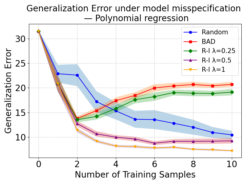
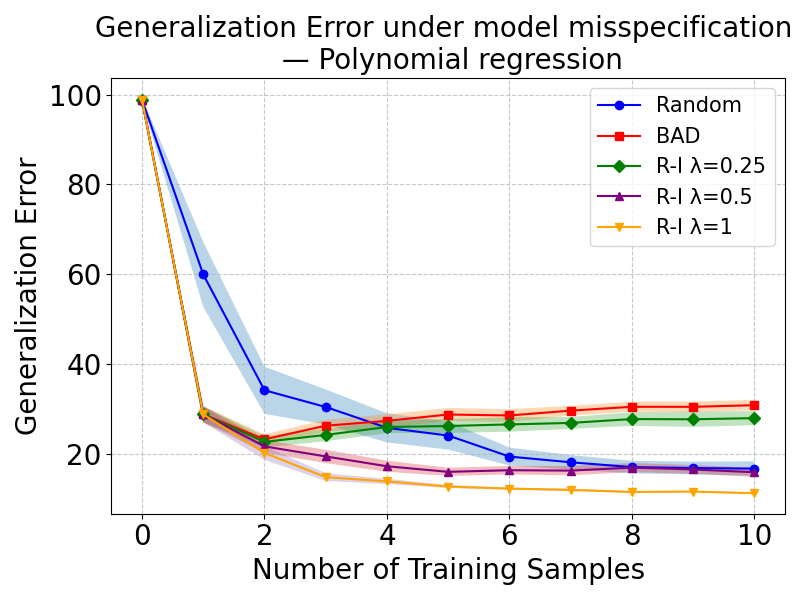
In the polynomial regression setting, the DGP is a degree-two polynomial regression model, $y=1+2x-0.5x^{2}+\epsilon$ where $\epsilon\sim\mathcal{N}(0,0.1)$. In the misspecified case, we use a linear model to fit the data this model generates. In the well-specified case, we use a quadratic model to fit the data this model generates. More implementational details are given in Section D.1, and more experimental results (one of which is in the well-specified case) can be found in Section E.1.

Figure 2 shows that under model misspecification, R-IDeA induces a higher degree of covariate shift than R-I, yet yields a better generalization error than R-I. This result suggests that generalization error performance is not influenced by the degree of covariate shift alone.

Moreover, R-I outperforms both BAD and Random, indicating that incorporating informativeness and representativeness leads to more effective design selection. R-IDeA further improves generalization performance and achieves the best results overall, demonstrating that jointly accounting for informativeness, representativeness, and de-amplification is most effective. Finally, R-IDeA-oracle, which uses the true $\bar{f}$ instead of the proxy $g$, as a baseline to validate the effectiveness of error de-amplification. And the results of R-IDeA perform comparably to R-IDeA-oracle, implying the R-IDeA is effective with the proxy $g$.

(a)

(b)

Figure 2: Comparison of different design strategies (Random, BAD, proposed R-I, proposed R-IDeA, and R-IDeA-oracle, which uses the true $\bar{f}$ instead of the proxy $g$) under misspecified models in both polynomial regression. Left: Generalization error across methods. Right: MMD distance across methods; higher values indicate a greater degree of covariate shift.

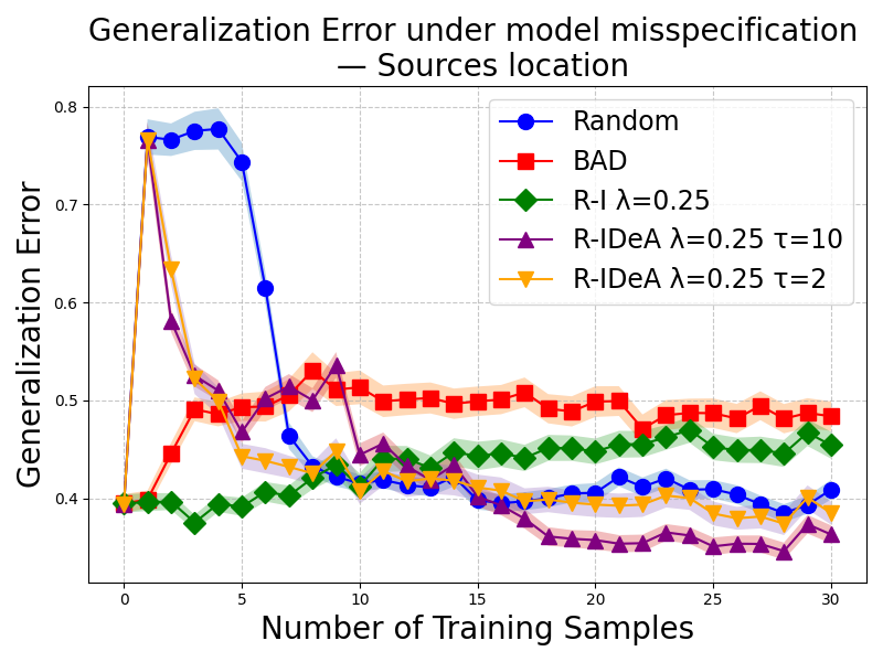
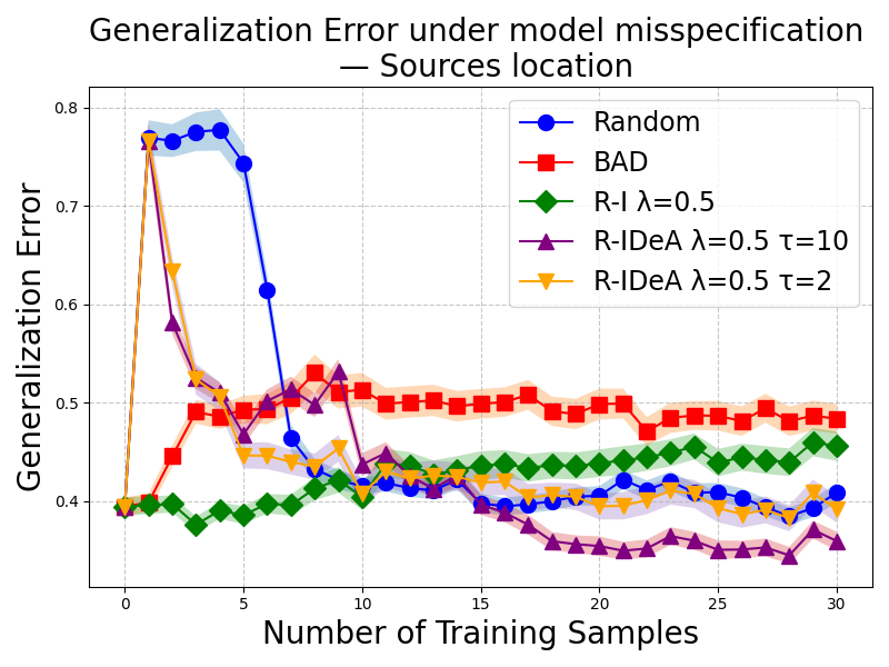
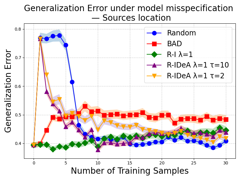
5.2 Source Localization Experiments

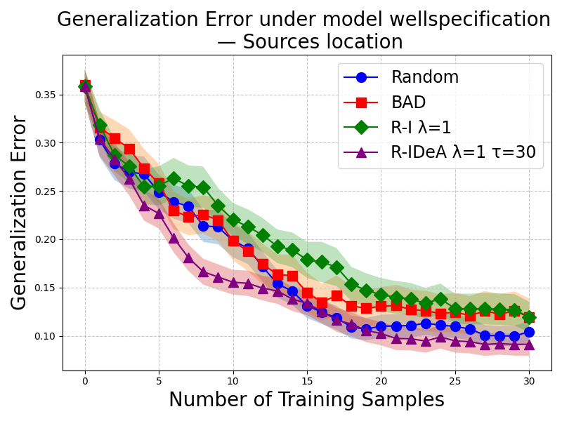
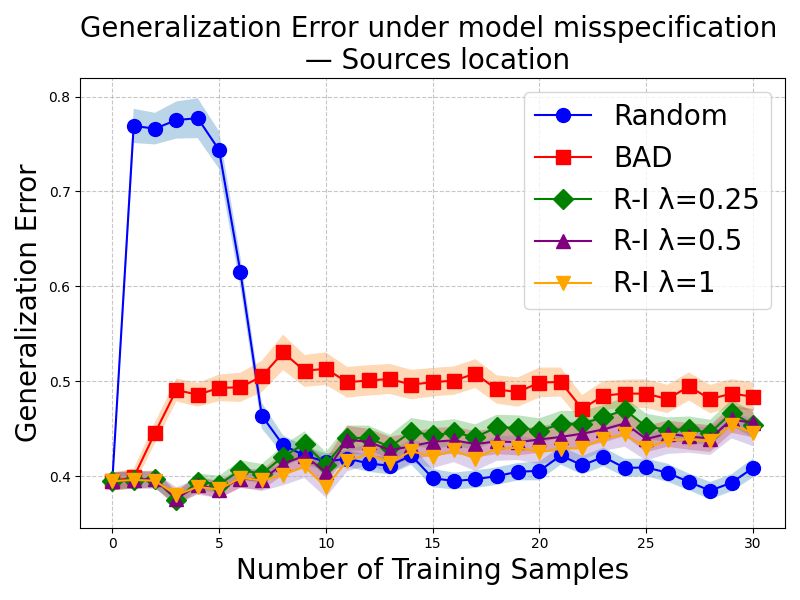
The acoustic energy attenuation model simulates the total intensity at location $\xi$ of a signal emitted from multiple sources at locations $\theta=\{\theta_{k}\}_{k=1}^{K}$. The objective of the design problem is to strategically select points at which to observe the total signal to infer the locations of the source effectively. More implementational details can be found in Section D.2, and more experimental results are in Section E.2.

Interestingly, under model misspecification, we observe that the generalization error of BAD and R-I slightly increases (Figure 3(a)) while the degree of covariate shift these methods induce decreases (Figure 3(b)). We speculate that this discrepancy is due to the amplifying properties of the designs selected by these methods. In the presence of model misspecification, R-I both outperform BAD and induce less covariate shift, suggesting the effectiveness of representative designs.

R-IDeA performs better than other methods and induces the highest covariate shift. This implies that covariate shift is not the only factor influencing generalization error, and that R-IDeA may perform better than other methods due to its selection of de-amplifying training data.

(a)

(b)

Figure 3: Comparison of baseline methods (Random, BAD) and our proposed R-I and R-IDeA in the source localization experiments. Top: Generalization error across methods. Bottom: MMD distance across methods; higher values indicate a greater degree of covariate shift.

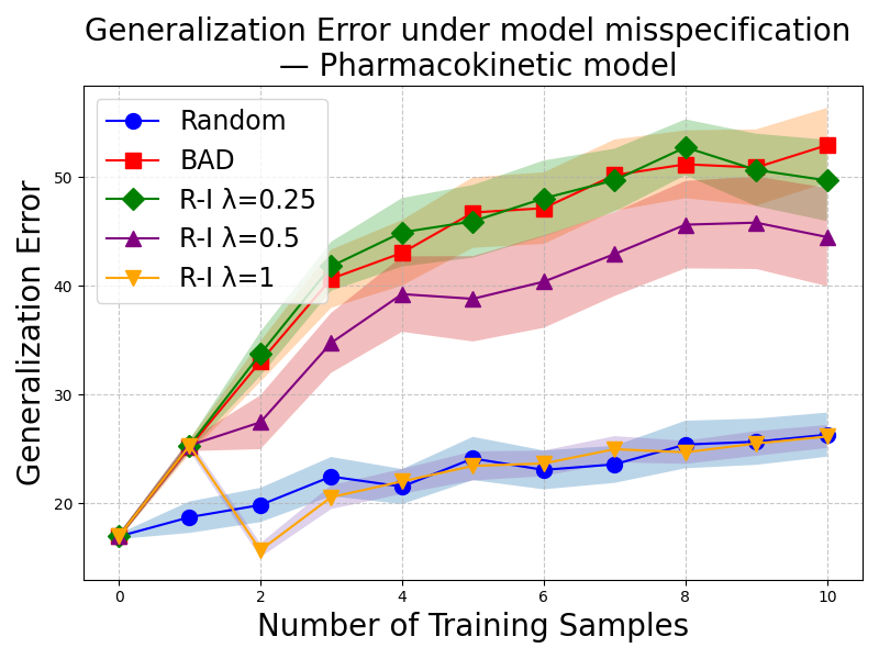
5.3 Pharmacokinetic Experiments

According to the Pharmacokinetic model, the distribution of an administered drug in the body is determined by three key parameters: the absorption rate $k_{\alpha}$, the elimination rate $k_{e}$, and the volume $V$. These define the parameter vector of interest, $\theta=(k_{\alpha},k_{e},V)$. The design task is to adaptively select blood sampling times $0\leq\xi_{t}\leq 24$ hours for each patient, measured from the moment of drug administration (with patient 2 receiving the drug only after collecting a sample from patient 1, and so on). More implementational details can be found in Section D.3, and more experimental results can be found in Section E.3.

Figure 4(a) shows that, under model misspecification, R-IDeA exhibits the best performance, suggesting that the selection of de-amplifying and representative designs can help reduce generalization error, consistent with the theoretical result established in Theorem 1. Figure 4(b) illustrates that in addition to exhibiting the best generalization performance, R-IDeA induces the largest degree of covariate shift, further demonstrating that designs that are de-amplifying in addition to representative contribute to robustness under model misspecification.

(a)

(b)

Figure 4: Comparison of baseline methods (Random, BAD) and our proposed R-I and R-IDeA in the Pharmacokinetic model experiments Top: Generalization error across methods. Bottom: MMD distance across methods; higher values indicate a greater degree of covariate shift.

6 CONCLUSION

When models are correctly specified, powerful experimental designs are informative about a parameter of interest. When models are misspecified, effective experimental designs are informative and robust to the misspecification. Our detailed analysis unpacks what is required for robustness. Our analysis reveals that robustness is a function of designs’ representativeness of the test distribution and de-amplification of misspecification errors. We leverage these insights to propose a novel method for BOED in the presence of potential model misspecification. Our empirical results demonstrate the effectiveness of the proposed method.

Limitations and Future Work A limitation of our work is that the main contributions are supported by insights from Theorem 1, which provides an upper bound on generalization performance. The degree to which this reflects actual generalization performance depends on the tightness of these bounds. Assessing the tightness of these bounds is therefore an important direction for future work. Moreover, the empirical results in Appendix E suggest that the properties of de-amplification, representativeness, and informativeness are not independent; rather, they are combined in the design. Consequently, tuning a hyperparameter to control one property will implicitly affect the others. This highlights the importance of selecting hyperparameters automatically and appropriately, rather than simply increasing or decreasing their values in a heuristic manner. Developing principled methods for automatic hyperparameter selection is an important direction for future work.

 

Supplementary Materials

 

Appendix A Proof of Proposition 1

$$R_{\mathrm{test}}(f) =\mathbb{E}_{\xi\sim d_{\text{test}}}\left[(f(\xi)-f^{\star}(\xi))^{2}\right]$$ (13)

$$=\mathbb{E}_{\xi\sim d_{\text{test}}}\left(\left(\left[f(\xi)-\bar{f}(\xi)\right]+\left[\bar{f}(\xi)-f^{\star}(\xi)\right]\right)^{2}\right)$$

$$=\underbrace{\mathbb{E}_{\xi\sim d_{\text{test}}}\left[(\bar{f}(\xi)-f^{\star}(\xi))^{2}\right]}_{\text{Misspecification Bias}}+\underbrace{\mathbb{E}_{\xi\sim d_{\text{test}}}\left[(f(\xi)-\bar{f}(\xi))^{2}\right]}_{\text{Estimation Bias}}$$

$$\quad+\underbrace{2\,\mathbb{E}_{\xi\sim d_{\text{test}}}\left[(\bar{f}(\xi)-f^{\star}(\xi))(f(\xi)-\bar{f}(\xi))\right]}_{\text{Error (De-)amplification}}.$$

Appendix B Proof of Theorem 1

Theorem: with probability at least $1-\delta$, the generalization error under covariate shift satisfies:

$$R_{\text{test}}(\hat{f}^{(n)})\leq\mathbb{C}_{\infty}\cdot\left\{\begin{aligned} &\mathbb{B}^{2}+\frac{224y_{\infty}^{2}\log(|\mathcal{F}|/\delta)}{3n}-2\widehat{\mathbb{A}}(\hat{f}^{(n)}),&\text{if }\widehat{\mathbb{A}}<0\\ &\mathbb{B}^{2}+\frac{128y_{\infty}^{2}\log(|\mathcal{F}|/\delta)}{3n}-\sqrt{3}\widehat{\mathbb{A}}(\hat{f}^{(n)}),&\text{if }\widehat{\mathbb{A}}\geq 0\end{aligned}\right.$$ (14)

Proof of Theorem

We provide the full derivation of the generalization error bound that preserves the error (de-)amplification term. Our analysis, which handles misspecification, is adapted from the proof of Proposition 2.1 in Amortila et al. (2024). In the proof, we first analyse the empirical error considering the training data distribution $d_{\text{train}}$, and then use the bounded density ratio to analyse the generalization error in the testing data distribution $d_{\text{test}}$.

The goal is to bound the generalization risk

$$R(f):=\mathbb{E}_{\xi}[(f(\xi)-f^{\star}(\xi))^{2}],$$

for any $f\in\mathcal{F}$. And the empirical risk is defined as:

$$\quad\widehat{R}(f):=\frac{1}{n}\sum_{i=1}^{n}\left(f\left(\xi_{i}\right)-y_{i}\right)^{2},$$

Observe that conditional on any $\xi$ we have:

$$\widehat{R}(f)-\widehat{R}(\bar{f})$$ (15)

$$=\mathbb{E}[(f\left.(\xi)-y)^{2}-(\bar{f}(\xi)-y)^{2}\mid\xi\right]$$

$$=\mathbb{E}\left[(f(\xi)-y)^{2}-\left(\bar{f}(\xi)-f^{\star}(\xi)+f^{\star}(\xi)-y\right)^{2}\mid\xi\right]$$

$$=\mathbb{E}\left[(f(\xi)-y)^{2}-\left(\bar{f}(\xi)-f^{\star}(\xi)\right)^{2}-2\left(\bar{f}(\xi)-f^{\star}(\xi)\right)\left(f^{\star}(\xi)-y\right)-\left(f^{\star}(\xi)-y\right)^{2}\mid\xi\right]$$

$$=\mathbb{E}\left[(f(\xi)-y)^{2}-\left(\bar{f}(\xi)-f^{\star}(\xi)\right)^{2}-\left(f^{\star}(\xi)-y\right)^{2}\mid\xi\right]$$

$$=f(\xi)^{2}-f^{\star}(\xi)^{2}-2\mathbb{E}_{\text{train }}[y\mid\xi]\left(f(\xi)-f^{\star}(\xi)\right)-\left(\bar{f}(\xi)-f^{\star}(\xi)\right)^{2}$$

$$=\left(f(\xi)-f^{\star}(\xi)\right)^{2}-\left(\bar{f}(\xi)-f^{\star}(\xi)\right)^{2}\quad(\text{since}\quad\mathbb{E}_{\text{train }}[y\mid\xi]=f^{\star}(\xi))$$

thus

$$\mathbb{E}(\widehat{R}(f)-\widehat{R}(\bar{f}))=\mathbb{E}(\left(f(\xi)-f^{\star}(\xi)\right)^{2}-\left(\bar{f}(\xi)-f^{\star}(\xi)\right)^{2})=R(f)-R(\bar{f})$$

And

$$\operatorname{Var}\left[(f(\xi)-y)^{2}-(\bar{f}(\xi)-y)^{2}\right]$$ (16)

$$=\mathbb{E}\left[\left((f(\xi)-y)^{2}-(\bar{f}(\xi)-y)^{2}\right)^{2}\right]-\left(\mathbb{E}\left[\left((f(\xi)-y)^{2}-(\bar{f}(\xi)-y)^{2}\right)\right]\right)^{2}\quad(\text{since}\quad\operatorname{Var}(X)=\mathbb{E}(X^{2})-(\mathbb{E}X)^{2})$$

$$\leq\mathbb{E}\left[\left((f(\xi)-y)^{2}-(\bar{f}(\xi)-y)^{2}\right)^{2}\right]$$

$$=\mathbb{E}\left[\left(f^{2}(\xi)-2f(\xi)y-\bar{f}^{2}(\xi)+2y\bar{f}(\xi)\right)^{2}\right]$$

$$=\mathbb{E}\left[(f(\xi)-\bar{f}(\xi))^{2}(f(\xi)+\bar{f}(\xi)-2y)^{2}\right]$$

$$\leq 6y_{\infty}^{2}\mathbb{E}\left[(f(\xi)-\bar{f}(\xi))^{2}\right]\quad\text{(since }|f(\xi)|,|\bar{f}(\xi)|,|y|\leq y_{\infty}\text{)}$$

$$=6y_{\infty}^{2}\mathbb{E}\left[(f(\xi)-f^{\star}(\xi)-(\bar{f}(\xi)-f^{\star}(\xi)))^{2}\right]$$

$$=6y_{\infty}^{2}\mathbb{E}\left[\left(f(\xi)-f^{\star}(\xi)\right)^{2}+\left(\bar{f}(\xi)-f^{\star}(\xi)\right)^{2}\right]-2y_{\infty}^{2}\mathbb{E}\left[(f(\xi)-f^{\star}(\xi))(\bar{f}(\xi)-f^{\star}(\xi))\right]$$

$$=6y_{\infty}^{2}\mathbb{E}\left[\left(f(\xi)-f^{\star}(\xi)\right)^{2}-\left(\bar{f}(\xi)-f^{\star}(\xi)\right)^{2}+2\left(\bar{f}(\xi)-f^{\star}(\xi)\right)^{2}\right]-2y_{\infty}^{2}\mathbb{E}\left[(f(\xi)-f^{\star}(\xi))(\bar{f}(\xi)-f^{\star}(\xi))\right]$$

$$=6y_{\infty}^{2}\mathbb{E}\left[\left(f(\xi)-f^{\star}(\xi)\right)^{2}-\left(\bar{f}(\xi)-f^{\star}(\xi)\right)^{2}+2\left(\bar{f}(\xi)-f^{\star}(\xi)\right)^{2}\right]$$

$$\quad-2y_{\infty}^{2}\mathbb{E}\left[(f(\xi)-\bar{f}(\xi)+\bar{f}(\xi)-f^{\star}(\xi))(\bar{f}(\xi)-f^{\star}(\xi))\right]$$

$$=6y_{\infty}^{2}\mathbb{E}\left[\left(f(\xi)-f^{\star}(\xi)\right)^{2}-\left(\bar{f}(\xi)-f^{\star}(\xi)\right)^{2}\right]+2y_{\infty}^{2}\mathbb{E}\left(\bar{f}(\xi)-f^{\star}(\xi)^{2}\right)$$

$$\quad-2y_{\infty}^{2}\mathbb{E}\left[(f(\xi)-\bar{f}(\xi))(\bar{f}(\xi)-f^{\star}(\xi))\right]-2y_{\infty}^{2}\mathbb{E}[(\bar{f}(\xi)-f^{\star}(\xi))^{2}]$$

$$\leq 6y_{\infty}^{2}\mathbb{E}\left[\left(f(\xi)-f^{\star}(\xi)\right)^{2}-\left(\bar{f}(\xi)-f^{\star}(\xi)\right)^{2}\right]-2y_{\infty}^{2}\underbrace{\mathbb{E}\left[(f(\xi)-\bar{f}(\xi))(\bar{f}(\xi)-f^{\star}(\xi))\right]}_{\widehat{\mathbb{A}}(f)}$$

$$=6y_{\infty}^{2}\mathbb{E}\left[\left(f(\xi)-f^{\star}(\xi)\right)^{2}-\left(\bar{f}(\xi)-f^{\star}(\xi)\right)^{2}\right]-2y_{\infty}^{2}\widehat{\mathbb{A}}(f)$$

$$=6y_{\infty}^{2}(R(f)-R(\bar{f}))-2y_{\infty}^{2}\widehat{\mathbb{A}}(f)$$

Application of Bernstein’s Inequality and Union Bound

Based on Bernstein’s inequality Shalev-Shwartz and Ben-David (2014) and union bound (see Lemma 2.2 in Shalev-Shwartz and Ben-David (2014)),

Bernstein’s inequality becomes:

$$\mathbf{P}\left(\mathbf{E}Z^{(f)}-\frac{1}{n}\sum_{i=1}^{n}Z^{(f)}_{i}<\frac{c}{3n}\log(|\mathcal{F}|/\delta)+\sqrt{\frac{2(\operatorname{Var}Z^{(f)})\log(|\mathcal{F}|/\delta)}{n}}\right)\geq 1-\delta$$

Setting $Z^{(f)}_{i}=(f(\xi)-y_{i})^{2}-(\bar{f}(\xi)-y_{i})^{2}$, thus $\frac{1}{n}\sum_{i=1}^{n}Z_{i}^{(f)}=\widehat{R}(f)-\widehat{R}(\bar{f});\quad\mathbb{E}Z^{(f)}=R(f)-R(\bar{f})$ , $|Z^{(f)}-EZ^{(f)}|\leq 2\sup|Z^{(f)}|\leq 2\sup(f(\xi)-y_{i})^{2}-(\bar{f}(\xi)-y_{i})^{2}=2\sup(f(\xi)-y_{i}+\bar{f}(\xi)-y_{i})(f(\xi)-\bar{f}(\xi))=2\cdot(4y_{\infty})(2y_{\infty})=c$, thus $c=16y_{\infty}^{2}$

Now, by using Bernstein’s inequality and a union bound over $f\in\mathcal{F}$ that with probability at least $1-\delta$

$$\forall f\in\mathcal{F}:R(f)-R(\bar{f})-(\widehat{R}(f)-\widehat{R}(\bar{f}))\leq\sqrt{\frac{\left(16(R(f)-R(\bar{f}))-32\widehat{\mathbb{A}}(f)\right)2y_{\infty}^{2}\log(|\mathcal{F}|/\delta)}{n}}+\frac{16y_{\infty}^{2}\log(|\mathcal{F}|/\delta)}{3n}.$$ (17)

Supppose the

$$\widehat{R}\left(\hat{f}^{(n)}\right)-\widehat{R}(\bar{f})\leq 0$$ (18)

we have

$$R\left(\hat{f}^{(n)}\right)-R(\bar{f}) \leq\sqrt{\frac{\left(16\left(R\left(\hat{f}^{(n)}\right)-R(\bar{f})\right)-32\widehat{\mathbb{A}}(\hat{f}^{(n)})\right)2y_{\infty}^{2}\log(|\mathcal{F}|/\delta)}{n}}+\frac{16y_{\infty}^{2}\log(|\mathcal{F}|/\delta)}{3n}$$ (19)

To simplify, make

$$A=R(\hat{f}^{(n)})-R(\bar{f})$$ (20)

$$C=y_{\infty}^{2}\frac{\log(|\mathcal{F}|/\delta)}{n}>0$$

Why $(16A-32\widehat{\mathbb{A}})\geq 0$

$$A =R(\hat{f}^{(n)})-R(\bar{f})=\mathbb{E}_{\xi}[(\hat{f}^{(n)}(\xi)-f^{\star}(\xi))^{2}]-\mathbb{E}_{\xi}[(\bar{f}(\xi)-f^{\star}(\xi))^{2}]$$ (21)

$$=\mathbb{E}_{\xi}[(\hat{f}^{(n)}(\xi)-f^{\star}(\xi)+\bar{f}(\xi)-f^{\star}(\xi))(\hat{f}^{(n)}(\xi)-\bar{f}(\xi))]$$

Then

$$1/2A-\widehat{\mathbb{A}} =1/2\mathbb{E}_{\xi}[(\hat{f}^{(n)}(\xi)-f^{\star}(\xi)+\bar{f}(\xi)-f^{\star}(\xi))(\hat{f}^{(n)}(\xi)-\bar{f}(\xi))]-\mathbb{E}_{\xi}\left[(\hat{f}^{(n)}-\bar{f}(\xi))(\bar{f}(\xi)-f^{\star}(\xi))\right]$$ (22)

$$=\mathbb{E}_{\xi}[(1/2\hat{f}^{(n)}(\xi)-1/2f^{\star}(\xi)+1/2\bar{f}(\xi)-1/2f^{\star}(\xi)-\bar{f}(\xi)+f^{\star}(\xi))(\hat{f}^{(n)}(\xi)-\bar{f}(\xi))]$$

$$=\mathbb{E}_{\xi}[(1/2\hat{f}^{(n)}(\xi)-1/2\bar{f}(\xi))(\hat{f}^{(n)}(\xi)-\bar{f}(\xi))]\geq 0$$

B.1 Suppose that $\widehat{\mathbb{A}}<0$

So the above inequality function equals:

$$A \leq\sqrt{(16A-32\widehat{\mathbb{A}})2C}+\frac{16C}{3}$$ (23)

$$\leq\sqrt{32AC}+\sqrt{-64\widehat{\mathbb{A}}C}+\frac{16C}{3}\quad(\text{since}\sqrt{a+b}<\sqrt{a}+\sqrt{b})$$

$$=\sqrt{A\cdot 32C}+\sqrt{-2\widehat{\mathbb{A}}\cdot 32C}+\frac{16C}{3}$$

$$\leq\frac{1}{2}A+6C-\widehat{\mathbb{A}}+6C+\frac{16C}{3}\quad(\sqrt{ab}\leq a/2+b/2)$$

$$=\frac{1}{2}A-\widehat{\mathbb{A}}+\frac{112C}{3}$$

so that

$$A\leq-2\widehat{\mathbb{A}}+\frac{224C}{3}$$ (24)

So

$$R\left(\hat{f}^{(n)}\right)-R(\bar{f})\leq-2\widehat{\mathbb{A}}(\hat{f}^{(n)})+\frac{224y_{\infty}^{2}\log(|\mathcal{F}|/\delta)}{3n}$$ (25)

Re-arranging and using that ${R}_{\text{train}}(\bar{f})\leq\mathbb{B}^{2}$, thus we have

$$R_{\text{train}}\left(\hat{f}^{(n)}\right)\leq\mathbb{B}^{2}-2\widehat{\mathbb{A}}(\hat{f}^{(n)})+\frac{224y_{\infty}^{2}\log(|\mathcal{F}|/\delta)}{3n}$$ (26)

Finally, let $\mathbb{C}_{\infty}:=\sup_{\xi\in\Xi}\left|\frac{d_{\text{test}}(\xi)}{d_{\text{train}}(\xi)}\right|$, the upper bound of generalization error can be expressed via the density ratio:

$$R_{\text{test}}\left(\hat{f}^{(n)}\right)=\mathbb{E}_{\text{train}}\left[\frac{d_{\text{test}}(\xi)}{d_{\text{train}}(\xi)}\left(\hat{f}^{(n)}(\xi)-f^{*}(\xi)\right)^{2}\right]\leq\mathbb{C}_{\infty}\cdot\left(\mathbb{B}^{2}-2\widehat{\mathbb{A}}(\hat{f}^{(n)})+\frac{224y_{\infty}^{2}\log(|\mathcal{F}|/\delta)}{3n}\right)$$ (27)

where $\widehat{\mathbb{A}}(\hat{f}^{(n)})=\mathbb{E}_{\text{train}}\left[(\hat{f}^{(n)}-\bar{f}(\xi))(\bar{f}(\xi)-f^{\star}(\xi))\right]$

B.2 Suppose that $\widehat{\mathbb{A}}\geq 0$

Although the second solution, based on solving a quadratic equation, yields a tighter upper bound, it involves more complex derivations. In contrast, the first solution offers a simpler and more interpretable decomposition, while preserving the same theoretical insights into the behavior of the error (de-)amplification term $\widehat{\mathbb{A}}(\hat{f}^{(n)})$. Therefore, we adopt the first formulation in the main text and provide the alternative quadratic-based bound in the appendix for completeness.

B.2.1 Solution 1: First order based upper bound derivation

Suppose that $\widehat{\mathbb{A}}\geq 0$ and $A>0$. We use the first-order upper bound for concave functions Boyd and Vandenberghe (2004):

$$\sqrt{a+b}\leq\sqrt{a}+\frac{b}{2\sqrt{a}}\quad\text{for }a>0,\ a+b\geq 0.$$

Since $(16A-32\widehat{\mathbb{A}})\geq 0$, thus $0\leq\widehat{\mathbb{A}}\leq 1/2A$

$$A \leq\sqrt{(16A-32\widehat{\mathbb{A}})2C}+\frac{16C}{3}$$ (28)

$$\leq\sqrt{32AC}-\frac{64\widehat{\mathbb{A}}C}{2\sqrt{32AC}}+\frac{16C}{3}$$

$$=\sqrt{A\cdot 32C}-\frac{4\sqrt{2}\widehat{\mathbb{A}}\sqrt{C}}{\sqrt{A}}+\frac{16C}{3}$$

$$\leq\frac{1}{2}A+6C-\frac{4\sqrt{2}\widehat{\mathbb{A}}\sqrt{C}}{\sqrt{A}}+\frac{16C}{3}\quad(\text{since}\sqrt{ab}\leq a/2+b/2)$$

$$=\frac{1}{2}A-\frac{4\sqrt{2}\widehat{\mathbb{A}}\sqrt{C}}{\sqrt{A}}+\frac{64C}{3}$$

$$\leq\frac{1}{2}A-\frac{4\sqrt{2}\widehat{\mathbb{A}}\sqrt{C}}{\sqrt{A_{max}}}+\frac{64C}{3}$$

so that

$$A \leq-\frac{8\sqrt{2}\widehat{\mathbb{A}}\sqrt{C}}{\sqrt{A_{max}}}+\frac{128C}{3}$$ (29)

$$=-\frac{8\sqrt{2}\widehat{\mathbb{A}}\sqrt{C}}{\sqrt{\frac{128C}{3}}}+\frac{128C}{3}\quad(\text{make}\widehat{\mathbb{A}}=0,\text{thus}A_{max}<\frac{128C}{3})$$

$$=\frac{128C}{3}-\sqrt{3}\widehat{\mathbb{A}}$$

thus:

$$R\left(\hat{f}^{(n)}\right)-R(\bar{f}) \leq\frac{128y_{\infty}^{2}\log(|\mathcal{F}|/\delta)}{3n}-\sqrt{3}\widehat{\mathbb{A}}$$ (30)

Re-arranging and using that ${R}_{\text{train}}(\bar{f})\leq\mathbb{B}^{2}$, thus we have

$$R_{train}\left(\hat{f}^{(n)}\right) \leq\mathbb{B}^{2}+\frac{128y_{\infty}^{2}\log(|\mathcal{F}|/\delta)}{3n}-\sqrt{3}\widehat{\mathbb{A}}$$ (31)

Finally, let $\mathbb{C}_{\infty}:=\sup_{\xi\in\Xi}\left|\frac{d_{\text{test}}(\xi)}{d_{\text{train}}(\xi)}\right|$, the upper bound of generalization error can be expressed via the density ratio:

$$R_{test}\left(\hat{f}^{(n)}\right) \leq\mathbb{C}_{\infty}\cdot\left(\mathbb{B}^{2}+\frac{128y_{\infty}^{2}\log(|\mathcal{F}|/\delta)}{3n}-\sqrt{3}\widehat{\mathbb{A}})\right)$$ (32)

where $\widehat{\mathbb{A}}(\hat{f}^{(n)})=\mathbb{E}_{\text{train}}\left[(\hat{f}^{(n)}-\bar{f}(\xi))(\bar{f}(\xi)-f^{\star}(\xi))\right]$

B.2.2 Solution 2: Quadratic-based upper bound derivation

Or solving the quadratic inequality $A\leq\sqrt{(16A-32\widehat{\mathbb{A}})2C}+\frac{16C}{3}$, thus

$$(A-\frac{16C}{3})^{2}\leq 2AC-4\widehat{\mathbb{A}}C$$ (33)

$$\Rightarrow A^{2}-\frac{32AC}{3}+(\frac{16C}{3})^{2}\leq 2AC-4\widehat{\mathbb{A}}C$$

$$\Rightarrow A^{2}-\frac{128AC}{3}+(\frac{16C}{3})^{2}+4\widehat{\mathbb{A}}C\leq 0$$

thus,

$$A\leq\frac{64C}{3}+\sqrt{\frac{1280C^{2}}{3}-64\widehat{\mathbb{A}}C}$$ (34)

here exists a solution if and only if$\frac{1280C^{2}}{3}-64\widehat{\mathbb{A}}C\geq 0$, which equals $\widehat{\mathbb{A}}\leq\frac{20C}{3}$

thus:

$$R\left(\hat{f}^{(n)}\right)-R(\bar{f}) \leq\frac{64y_{\infty}^{2}\log(|\mathcal{F}|/\delta)}{3n}+\sqrt{\frac{1280y_{\infty}^{4}[\log(|\mathcal{F}|/\delta)]^{2}}{3n^{2}}-\frac{64\widehat{\mathbb{A}}y_{\infty}^{2}\log(|\mathcal{F}|/\delta)}{n}}$$ (35)

Re-arranging and using that ${R}_{\text{train}}(\bar{f})\leq\mathbb{B}^{2}$, thus we have

$$R_{train}\left(\hat{f}^{(n)}\right) \leq\mathbb{B}^{2}+\frac{64y_{\infty}^{2}\log(|\mathcal{F}|/\delta)}{3n}+\sqrt{\frac{1280y_{\infty}^{4}[\log(|\mathcal{F}|/\delta)]^{2}}{3n^{2}}-\frac{64\widehat{\mathbb{A}}y_{\infty}^{2}\log(|\mathcal{F}|/\delta)}{n}}$$ (36)

Finally, let $\mathbb{C}_{\infty}:=\sup_{\xi\in\Xi}\left|\frac{d_{\text{test}}(\xi)}{d_{\text{train}}(\xi)}\right|$, the upper bound of generalization error can be expressed via the density ratio:

$$R_{test}\left(\hat{f}^{(n)}\right) \leq\mathbb{C}_{\infty}\cdot\left(\mathbb{B}^{2}+\frac{64y_{\infty}^{2}\log(|\mathcal{F}|/\delta)}{3n}+\sqrt{\frac{1280y_{\infty}^{4}[\log(|\mathcal{F}|/\delta)]^{2}}{3n^{2}}-\frac{64\widehat{\mathbb{A}}y_{\infty}^{2}\log(|\mathcal{F}|/\delta)}{n}})\right)$$ (37)

where $\widehat{\mathbb{A}}(\hat{f}^{(n)})=\mathbb{E}_{\text{train}}\left[(\hat{f}^{(n)}-\bar{f}(\xi))(\bar{f}(\xi)-f^{\star}(\xi))\right]$

B.3 loosen the $\widehat{\mathbb{A}}$

We reproduce this derivation for completeness, following the approach in Amortila et al. (2024), although it is not directly used in our main results.

In the inequality 16, we keep the interaction term $\widehat{\mathbb{A}}$. and if we loose the $\widehat{\mathbb{A}}$ by using the AM-GM inequality $\left((a+b)^{2}\leq 2a^{2}+2b^{2}\right)$, the above equation becomes :

$$\operatorname{Var}\left[(f(\xi)-y)^{2}-(\bar{f}(\xi)-y)^{2}\right]$$ (38)

$$=\mathbb{E}\left[\left((f(\xi)-y)^{2}-(\bar{f}(\xi)-y)^{2}\right)^{2}\right]-\left(\mathbb{E}\left[\left((f(\xi)-y)^{2}-(\bar{f}(\xi)-y)^{2}\right)\right]\right)^{2}$$

$$\leq\mathbb{E}\left[\left((f(\xi)-y)^{2}-(\bar{f}(\xi)-y)^{2}\right)^{2}\right]$$

$$=\mathbb{E}\left[\left(f^{2}(\xi)-2f(\xi)y-\bar{f}^{2}(\xi)+2y\bar{f}(\xi)\right)^{2}\right]$$

$$=\mathbb{E}\left[(f(\xi)-\bar{f}(\xi))^{2}(f(\xi)+\bar{f}(\xi)-2y)^{2}\right]$$

$$\leq 6y_{\infty}^{2}\mathbb{E}\left[(f(\xi)-\bar{f}(\xi))^{2}\right]\quad\text{(since }|f(\xi)|,|\bar{f}(\xi)|,|y|\leq y_{\infty}\text{)}$$

$$=6y_{\infty}^{2}\mathbb{E}\left[(f(\xi)-f^{\star}(\xi)+f^{\star}(\xi)-\bar{f}(\xi))^{2}\right]$$

$$\leq 2y_{\infty}^{2}\mathbb{E}\left[((f(\xi)-f^{\star}(\xi))^{2}+(\bar{f}(\xi)-f^{\star}(\xi))^{2})\right]\quad\text{(since }(a+b)^{2}\leq 2a^{2}+2b^{2})$$

$$=2y_{\infty}^{2}\mathbb{E}\left[\left(f(\xi)-f^{\star}(\xi)\right)^{2}-\left(\bar{f}(\xi)-f^{\star}(\xi)\right)^{2}+2\left(\bar{f}(\xi)-f^{\star}(\xi)\right)^{2}\right]$$

$$\leq 2y_{\infty}^{2}\mathbb{E}\left[\left(f(\xi)-f^{\star}(\xi)\right)^{2}-\left(\bar{f}(\xi)-f^{\star}(\xi)\right)^{2}\right]+4y_{\infty}^{2}\mathbb{B}^{2}$$

$$=2y_{\infty}^{2}(R(f)-R(\bar{f}))+4y_{\infty}^{2}\mathbb{B}^{2}$$

Using the same logic in the above derivation, based on the LABEL:equ:loosA, we have:

$$A \leq\sqrt{(32A+64B)2C}+\frac{16C}{3}$$ (39)

$$\leq\sqrt{64AC}+\sqrt{128BC}+\frac{16C}{3}\quad(\text{since}\sqrt{a+b}<\sqrt{a}+\sqrt{b})$$

$$=\sqrt{A\cdot 64C}+\sqrt{2B\cdot 64C}+\frac{16C}{3}$$

$$\leq\frac{1}{2}A+2C+B+2C+\frac{16C}{3}\quad(\text{since}\sqrt{ab}\leq a/2+b/2)$$

$$=\frac{1}{2}A+B+\frac{208C}{3}$$

so that

$$A\leq 2B+\frac{416C}{3}$$ (40)

So

$$R\left(\hat{f}^{(n)}\right)-R(\bar{f})\leq 2\mathbb{B}^{2}+\frac{416y_{\infty}^{2}\log(|\mathcal{F}|/\delta)}{3n}$$ (41)

Re-arranging and using that ${R}_{\text{train}}(\bar{f})\leq\mathbb{B}^{2}$, thus we have

$$R_{\text{train}}\left(\hat{f}^{(n)}\right)\leq 3\mathbb{B}^{2}+\frac{416y_{\infty}^{2}\log(|\mathcal{F}|/\delta)}{3n}$$ (42)

Let $\mathbb{C}_{\infty}:=\sup_{\xi\in\Xi}\left|\frac{d_{\text{test}}(\xi)}{d_{\text{train}}(\xi)}\right|$, the upper bound of generalization error can be expressed via the density ratio:

$$R_{\text{test}}\left(\hat{f}^{(n)}\right)=\mathbb{E}_{\text{train}}\left[\frac{d_{\text{test}}(\xi)}{d_{\text{train}}(\xi)}\left(\hat{f}^{(n)}(\xi)-f^{*}(\xi)\right)^{2}\right]\leq\mathbb{C}_{\infty}\cdot\left(3\mathbb{B}^{2}+\frac{416y_{\infty}^{2}\log(|\mathcal{F}|/\delta)}{3n}\right)$$ (43)

Appendix C Constructing the approximate/proxy de-amplifying region

C.1 Proof of Theorem 2

Theorem 2 [Approximate de-amplifying region] Let $\bar{f}$ be the predictor that best approximates the true data-generating function $f^{\star}$ in expectation with respect to the test distribution. Then,

$$\widehat{\Xi}_{\mathbb{A}+}(\tau)\subseteq\Xi_{\mathbb{A}+}(\tau_{0})$$

where the approximate de-amplifying region $\widehat{\Xi}_{\mathbb{A}+}(\tau)\coloneqq\Big\{\xi:|\hat{f}^{(n)}(\xi)-\bar{f}(\xi)|\geq\tau\Big\}$, $\tau=\tau_{0}/\mathbb{B}_{\infty}+c\mathbb{B}_{\infty}$, $c\geq 2$, and $\tau_{0}\geq 0$.

Proof Sketch:

To compute a subset of $\Big\{\xi:(\hat{f}^{(n)}(\xi)-\bar{f}(\xi))(\bar{f}(\xi)-f^{\star}(\xi))\geq\tau_{0}\Big\}$ and remove the dependence on $f^{\star}$, we instead construct a subset of the de-amplifying region, the approximate de-amplifying region:

$$\Big\{\xi:|\hat{f}^{(n)}(\xi)-\bar{f}(\xi)|\geq c\mathbb{B}_{\infty}+\tau_{0}/\mathbb{B}_{\infty},\;c\geq 2,\tau_{0}\geq 0\Big\}\subseteq\Big\{\xi:(\hat{f}^{(n)}(\xi)-\bar{f}(\xi))(\bar{f}(\xi)-f^{\star}(\xi))\geq\tau_{0}\Big\}.$$ (44)

Below, we detail the derivation of each of the following subset relations:

$$\widehat{\Xi}_{\mathbb{A}+}(\tau) =\Big\{\xi:|\hat{f}^{(n)}(\xi)-\bar{f}(\xi)|\geq c\mathbb{B}_{\infty}+\tau_{0}/\mathbb{B}_{\infty},\;c\geq 2,\tau_{0}\geq 0\Big\}$$

$$\subseteq^{(i)}\Big\{\xi:|\hat{f}^{(n)}(\xi)-f^{\star}(\xi)|\geq\tau_{0}/\mathbb{B}_{\infty}+\mathbb{B}_{\infty},\tau_{0}\geq 0\Big\}$$

$$\subseteq^{(ii)}\Big\{\xi:|\hat{f}^{(n)}(\xi)-f^{\star}(\xi)|-|\bar{f}(\xi)-f^{\star}(\xi)|\geq\tau_{0}/\mathbb{B}_{\infty},\tau_{0}\geq 0\Big\}$$

$$\subseteq^{(iii)}\Big\{\xi:(\hat{f}^{(n)}(\xi)-\bar{f}(\xi))(\bar{f}(\xi)-f^{\star}(\xi))\geq\tau_{0}\Big\}$$

$$=\Xi_{\mathbb{A}+}(\tau_{0})$$

Proof of subset relation (iii)

We would design an acquisition function that selects only designs in the de-amplifying region $\Xi_{\mathbb{A}+}(\tau_{0})$, where $\Xi_{\mathbb{A}+}(\tau_{0})\coloneqq\Big\{\xi:(\hat{f}^{(n)}(\xi)-\bar{f}(\xi))(\bar{f}(\xi)-f^{\star}(\xi))\geq\tau_{0}\Big\}$. And the left side of the inequality can be expressed as below:

$$(\hat{f}^{(n)}(\xi)-\bar{f}(\xi))(\bar{f}(\xi)-f^{\star}(\xi))$$ (45)

$$=(\hat{f}^{(n)}(\xi)-f^{\star}(\xi)+f^{\star}(\xi)-\bar{f}(\xi))(\bar{f}(\xi)-f^{\star}(\xi))$$

$$=(\hat{f}^{(n)}(\xi)-f^{\star}(\xi))(\bar{f}(\xi)-f^{\star}(\xi))-(\bar{f}(\xi)-f^{\star}(\xi))^{2}$$

Thus, we refer to a design $\xi$ as de-amplifying whenever $(\hat{f}^{(n)}(\xi)-\bar{f}(\xi))(\bar{f}(\xi)-f^{\star}(\xi))=(\hat{f}^{(n)}(\xi)-f^{\star}(\xi))(\bar{f}(\xi)-f^{\star}(\xi))-(\bar{f}(\xi)-f^{\star}(\xi))^{2}\geq\tau_{0}$ for a given threshold $\tau_{0}$.

Make an assumption that $\tau_{0}\geq 0$, and based on $|\bar{f}(\xi)-f^{\star}(\xi)|<\mathbb{B}_{\infty}$, thus we have

$$|\hat{f}^{(n)}(\xi)-f^{\star}(\xi)|-|\bar{f}(\xi)-f^{\star}(\xi)|\geq\tau_{0}/|\bar{f}(\xi)-f^{\star}(\xi)|\geq\tau_{0}/\mathbb{B}_{\infty},$$

the subset (iii) follows.

Proof of subset relation (ii)

From $\Big\{\xi:|\hat{f}^{(n)}(\xi)-f^{\star}(\xi)|-|\bar{f}(\xi)-f^{\star}(\xi)|\geq\tau_{0}/\mathbb{B}_{\infty}\Big\}$ we obtain

$$\Big\{\xi:|\hat{f}^{(n)}(\xi)-f^{\star}(\xi)|\geq\tau_{0}/\mathbb{B}_{\infty}+|\bar{f}(\xi)-f^{\star}(\xi)|\Big\}.$$

Since $|\bar{f}(\xi)-f^{\star}(\xi)|\leq\mathbb{B}_{\infty}$, it follows that

$$\Big\{\xi:|\hat{f}^{(n)}(\xi)-f^{\star}(\xi)|\geq\tau_{0}/\mathbb{B}_{\infty}+\mathbb{B}_{\infty}\Big\}\subseteq\Big\{\xi:|\hat{f}^{(n)}(\xi)-f^{\star}(\xi)|-|\bar{f}(\xi)-f^{\star}(\xi)|\geq\tau_{0}/\mathbb{B}_{\infty}\Big\}.$$

Proof of subset relation (i)

Making a assumption that $\{\xi:|\hat{f}^{(n)}(\xi)-\bar{f}(\xi)|\geq c\mathbb{B}_{\infty}+\tau_{0}/\mathbb{B}_{\infty}\}$ holds, then

$$|\hat{f}^{(n)}(\xi)-f^{\star}(\xi)|=|\hat{f}^{(n)}(\xi)-\bar{f}(\xi)+\bar{f}(\xi)-f^{\star}(\xi)|\geq|\hat{f}^{(n)}(\xi)-\bar{f}(\xi)|-|f^{\star}(\xi)-\bar{f}(\xi)|\geq(c-1)\mathbb{B}_{\infty}+\tau_{0}/\mathbb{B}_{\infty}.$$

Combining this with $\Big\{\xi:|\hat{f}^{(n)}(\xi)-f^{\star}(\xi)|\geq\tau_{0}/\mathbb{B}_{\infty}+\mathbb{B}_{\infty}\Big\}$, we see that for $c\geq 2$, subset (i) follows.

C.2 Proof of Lemma 1

Lemma 1 [Proxy region approximates $\widehat{\Xi}_{\mathbb{A}+}(\tau)$] Assume $\sup_{\xi\in\Xi}|g(\xi)-\bar{f}(\xi)|\leq\tau_{2}$ for some $\tau_{2}\geq 0$. Then

$$\big\{\xi:\,|\hat{f}^{(n)}(\xi)-g(\xi)|\geq\tau+\tau_{2}\big\}\;\subseteq\;\widehat{\Xi}_{\mathbb{A}+}(\tau).$$

Proof. By the triangle inequality,

$$|\hat{f}^{(n)}(\xi)-\bar{f}(\xi)|\geq|\hat{f}^{(n)}(\xi)-g(\xi)|-|g(\xi)-\bar{f}(\xi)|\geq|\hat{f}^{(n)}(\xi)-g(\xi)|-\tau_{2}$$

Thus when

$$|\hat{f}^{(n)}(\xi)-g(\xi)|\geq\tau+\tau_{2},$$

we have

$$|\hat{f}^{(n)}(\xi)-\bar{f}(\xi)|\geq|\hat{f}^{(n)}(\xi)-g(\xi)|-\tau_{2}\geq\tau\Rightarrow|\hat{f}^{(n)}(\xi)-\bar{f}(\xi)|\geq\tau$$

So

$$\big\{\xi:\,|\hat{f}^{(n)}(\xi)-g(\xi)|\geq\tau+\tau_{2}\big\}\;\subseteq\;\widehat{\Xi}_{\mathbb{A}+}(\tau).$$

Appendix D Additional Details of the Numerical Experiments

Our experiments were implemented using PyTorch Paszke (2019) and Pyro Bingham et al. (2019). All experiments were conducted on a shared computing cluster using NVIDIA A100 GPUs. Each job was allocated one A100 GPU, 8 CPU cores, and 32GB of RAM.

Measuring the degree of covariate shift

To measure the distance between the distributions or datasets, we use the Maximum mean discrepancy (MMD). A number of advantages of this distance are put forward in the literature: 1) it is more robust to outliers than other discrepancy measurements (like KL divergence) Gretton et al. (2012); 2) it can be approximated on the basis of differently-sized samples from the distributions being compared Gretton et al. (2012); 3) the measurement is robust to repeated samples (unlike the Wasserstein distance) Viehmann (2021); 4) the measurement can be computed efficiently using samples Bharti et al. (2023); Huang et al. (2023).

We compute the squared Maximum Mean Discrepancy (MMD) Gretton et al. (2012) between two empirical distributions $\mathcal{P}=\{p_{i}\}_{i=1}^{m}$ and $\mathcal{Q}=\{q_{j}\}_{j=1}^{n}$ using the Gaussian (RBF) kernel:

$$\mathrm{MMD}^{2}(\mathcal{P},\mathcal{Q})=\frac{1}{m^{2}}\sum_{i=1}^{m}\sum_{i^{\prime}=1}^{m}k(p_{i},p_{i^{\prime}})+\frac{1}{n^{2}}\sum_{j=1}^{n}\sum_{j^{\prime}=1}^{n}k(q_{j},q_{j^{\prime}})-\frac{2}{mn}\sum_{i=1}^{m}\sum_{j=1}^{n}k(p_{i},q_{j}),$$

where $k(p,q)=\exp\!\left(-\tfrac{\|p-q\|^{2}}{2\sigma^{2}}\right)$ is the RBF kernel with fixed bandwidth $\sigma=1$.

Measuring the generalization performance

To evaluate the generalization performance, we compute the Mean Squared Error (MSE) between the model predictions $\hat{f}^{(n)}$ and the corresponding true observations from the data-generating process (DGP) $y$, given the test samples.

$$\mathrm{MSE}=\frac{1}{D}\sum_{d=1}^{D}\frac{1}{N}\sum_{i=1}^{N}(\hat{f}^{(n)}_{d,i}-y_{d,i})^{2}$$

where D is the number of test samples, and N is the sampling number.

D.1 Polynomial regression experiments

Both well-specified and misspecified models were run across 20 runs. For each run, the design is adaptively selected, and the total number of designs is $T=10$.

Well-specified case

• DGP: The DGP is a degree-two polynomial regression model, $y=1+2x-0.5x^{2}+\epsilon$ where $\epsilon\sim\mathcal{N}(0,0.1)$

• well-specified model: $f(x)=\beta_{0}+\beta_{1}x+\beta_{2}x^{2}$ So the feature functions are $\phi(x)=[1,x,x^{2}]^{\top}$

• Test distribution (arbitrary $\mathbf{\xi}^{test}$): $\mathbf{\xi}^{test}\sim\mathcal{U}(-4,4)$

Misspecified case

• DGP: The DGP is a degree-two polynomial regression model, $y=1+2x-0.5x^{2}+\epsilon$ where $\epsilon\sim\mathcal{N}(0,0.1)$

• misspecified model: $f(x)=\beta_{0}+\beta_{1}x$ So the feature functions are $\phi(x)=[1,x]^{\top}$

• Test distribution (arbitrary $\mathbf{\xi}^{test}$): $\mathbf{\xi}^{test}\sim\mathcal{U}(-4,4)$

D.2 Source localization experiments

We take $T=30$ iteration steps for selecting training samples $\mathbf{\xi}^{train}$ and 200 test samples for the observed $f^{\star}(\mathbf{\xi}^{test})$ and predicted output $f(\mathbf{\xi}^{test})$. We set $K=2$ sources and limit the range of design to $\mathbf{\xi}^{train}\in[-4,4]$. We use 200 samples drawn from the uniform distribution over $\mathbf{\xi}^{test}\in[-4,4]$ as the test distribution to estimate the MMD.

In this experiment, we have $K$ sources with unknown location parameter is $\theta=\{\theta_{k}\}_{k=1}^{K}$. We assume the number of sources $K$ is known.

Acoustic energy attenuation model

The total intensity, a superposition of the individual ones, at location $\xi$ from $K$ sources is considered in the following equation Foster et al. (2021); Ivanova et al. (2024):

$$\mu(\theta,\xi)=b+\sum_{k=1}^{K}\frac{\alpha_{k}}{m+\left\|\theta_{k}-\xi\right\|^{2}}$$ (46)

The prior distribution of each location parameter $\theta_{k}$ is a normal distribution, and the observation noise is Gaussian noise. Therefore, the prior and likelihood are in the following:

$$\theta_{k}\stackrel{{\scriptstyle\text{ i.i.d. }}}{{\sim}}N\left(0_{d},I_{d}\right),\log y\mid\theta,\xi\sim N(\log\mu(\theta,\xi),\sigma)$$

Well-specfied case

The hyperparameters of the true DGP used in our well-specification experiments can be found in the table below:

$$\begin{array}[]{lr}\text{ Parameter }&\text{ Value }\\ \hline\cr\text{ Number of sources, }K&2\\ \text{ Base signal, }b&10^{-1}\\ \text{ Max signal, }m&10^{-4}\\ \alpha_{1},\alpha_{2}&1\\ \text{ Signal noise, }\sigma&0.1\end{array}$$

The model hyperparameters used in our experiments are the same in the above table.

Misspecfied case

The hyperparameters of the true DGP used in our mis-specification experiments can be found in the table below:

$$\begin{array}[]{lr}\text{ Parameter }&\text{ Value }\\ \hline\cr\text{ Number of sources, }K&2\\ \text{ Base signal, }b&4*10^{-1}\\ \text{ Max signal, }m&4*10^{-4}\\ \alpha_{1},\alpha_{2}&0.4\\ \text{ Signal noise, }\sigma&0.1\end{array}$$

The model hyperparameters used in our experiments are the same as the table in the well-specified case.

D.3 Pharmacokinetic model

We take $T=10$ iteration steps for selecting training samples $\mathbf{\xi}^{train}$ and 200 test samples for the observed $f^{\star}(\mathbf{\xi}^{test})$ and predicted output $f(\mathbf{\xi}^{test})$. We limit the range of design to $\mathbf{\xi}^{train}\in[0,24]$. We use 200 samples drawn from the uniform distribution over $\mathbf{\xi}^{test}\in[0,24]$ as the test distribution to estimate the MMD. In the experiment, we set the true theta as $\theta_{\text{real}}=[1.5,0.15,15.0]$

Well–specified case.

The drug concentration $z$, measured $\xi$ hours after administration, and the corresponding noisy observation $y$, are modeled as

$$z(\xi;\theta)=\frac{D_{V}}{V}\cdot\frac{k_{\alpha}}{k_{\alpha}-k_{e}}\left[e^{-k_{e}\xi}-e^{-k_{\alpha}\xi}\right],\qquad y(\xi;\theta)=z(\xi;\theta)(1+\epsilon)+\eta,$$ (47)

where $\theta=(k_{\alpha},k_{e},V)$, $D_{V}=400$ is a constant, $\epsilon\sim\mathcal{N}(0,0.01)$ is multiplicative noise (to capture heteroscedasticity), and $\eta\sim\mathcal{N}(0,0.1)$ is additive observation noise.

The prior distribution for the parameters $\theta$ is specified as

$$\log\theta\sim\mathcal{N}\!\left(\begin{bmatrix}\log 1\\ \log 0.1\\ \log 20\end{bmatrix},\begin{bmatrix}0.05&0&0\\ 0&0.05&0\\ 0&0&0.05\end{bmatrix}\right).$$ (48)

Since both noise sources are Gaussian, the observation likelihood and DGP are the same and are also Gaussian:

$$y(\xi;\theta)\sim\mathcal{N}\!\big(z(\xi;\theta),\;0.01\,z(\xi;\theta)^{2}+0.1\big),$$ (49)

Misspecified case.

To introduce model misspecification, DGP comes from Equation 49. And a dual–absorption model with two parallel absorption rates is generated to make a prediction. Let $k_{a1}=k_{\alpha}$ and $k_{a2}=\rho\,k_{a1}$ with $\rho\in(0,1)$, and let $f\in(0,1)$ denote the fraction of the fast pathway. The mean concentration is

$$z_{\text{pre}}(\xi;\theta,\rho,f)=\tfrac{D_{V}}{V}\!\left[f\cdot\tfrac{k_{a1}}{k_{a1}-k_{e}}\big(e^{-k_{e}\xi}+e^{-k_{a1}\xi}\big)+(1-f)\cdot\tfrac{k_{a2}}{k_{a2}-k_{e}}\big(e^{-k_{e}\xi}+e^{-k_{a2}\xi}\big)\right].$$ (50)

We set $\rho=0.25$ and $f=0.6$. The observation in the assumed model is,

$$y_{\text{pre}}(\xi;\theta)\sim\mathcal{N}\!\big(z_{\text{pre}}(\xi;\theta,\rho,f),\;0.02\,z_{\text{pre}}(\xi;\theta,\rho,f)^{2}+0.2\big).$$

Appendix E Additional Results of the Numerical Experiments

E.1 Polynomial Regression Experiments

E.1.1 Model Well-specification

Figure 5 shows that, in the well-specified case, all methods yield similar generalization error (Figure 5(a)), regardless of the degree of covariate shift (Figure 5(b)). This indicates that covariate shift does not significantly impact generalization performance when the model is well-specified. Moreover, the proposed R-I acquisition function, which combines informativeness and representativeness, converges more quickly than random selection. The proposed R-IDeA acquisition function successfully selects de-amplifying designs, yielding faster improvements in generalization compared to random. And R-IDeA have comparable results with R-IDeA-oracle which uses the $\bar{f}$ instead of the proxy $g$, demonstrating that R-IDeA is effective with proxy $g$.

(a)

(b)

Figure 5: Comparison of different design strategies (Random, BAD, proposed R-I, proposed R-IDeA, and R-IDeA-oracle under well-specified models in polynomial regression. Left: Generalization error across methods. Right: MMD distance across methods; higher values indicate a greater degree of covariate shift.

E.1.2 Model Misspecification

R-I - varying $\lambda$

Figures 6(a) and 6(b) show the performance of the proposed R-I acquisition function under various values of $\lambda$. For larger values of $\lambda$, we expect the representativeness term to dominate the acquisition function, resulting in a design distribution that resembles the test distribution. Figure 6(b) shows that when designs are more representative, generalization error is reduced (Figure 6(a)), consistent with the theoretical prediction introduced in Theorem 1. These results demonstrate again that representative designs effectively reduce estimation bias and improve generalization performance.

(a)

(b)

Figure 6: Comparison of baseline methods (Random, BAD) and our proposed R-I with varying $\lambda$ in the polynomial regression experiments Left: Generalization error across methods. Right: MMD distance across methods; higher values indicate a greater degree of covariate shift.

R-IDeA - varying $\tau$

Figure 7 show the performance of our R-IDeA acquisition function under various learned adversarial proxies with different values of $\tau$. Over all values of $\tau$, R-IDeA has a higher generalization performance than R-I, suggesting that de-amplifying designs with error-(de)amplifying property indeed increase generalization performance.

From Equation 11 and Equation 12, we see that larger values of $\tau$ result in design distributions with stricter de-amplifying constraints. In other words, when $\tau$ is large, we expect the de-amplifying term to dominate the acquisition function. For smaller values of $\tau$, the de-amplifying constraint is loosened, resulting in more candidate designs being effectively considered as part of the de-amplifying region. Therefore, $\tau$ should be chosen to balance de-amplification and other properties (informativeness and representativeness).

Moreover, Figure 7(a), Figure 7(c) and Figure 7(e) show that when $\tau=0.5$, R-IDeA performs better than under other values of $\tau$. This demonstrates the importance of balancing de-amplification with other properties. We leave the development of systematic methods for selecting the hyperparameters in R-I and R-IDeA for future work.

(a)

(b)

(c)

(d)

(e)

(f)

Figure 7: Comparison of baseline methods (Random, BAD), our proposed R-I and our proposed R-IDeA with varying $\tau$ in the polynomial regression experiments. Rows correspond to variation in $\lambda$. Left: Generalization error across methods. Right: MMD distance across methods; higher values indicate a greater degree of covariate shift.

E.1.3 High Degrees of Misspecification

In the discussion before, we included the no-misspecification and mild-misspecification settings (quadratic DGP). To investigate the impact of the proposed acquisition function under different levels of misspecification, we also ran the experiments with a higher degree of misspecification by adding the cubic term to the DGP (we set DGP is $y=1+2x-0.5x^{2}+0.2x^{3}+\epsilon$ where $\epsilon\sim\mathcal{N}(0,0.1)$). The results (see Figure 8 and Figure 9) show a similar trend: R-I and R-IDeA continue to provide stable and competitive performance even as misspecification increases.

(a)

(b)

Figure 8: Comparison of baseline methods (Random, BAD) and our proposed R-I with varying $\lambda$ in the three degree of polynomial regression experiments Left: Generalization error across methods. Right: MMD distance across methods; higher values indicate a greater degree of covariate shift.

(a)

(b)

(c)

(d)

(e)

(f)

Figure 9: Comparison of baseline methods (Random, BAD), our proposed R-I and our proposed R-IDeA with varying $\tau$ in the three degree polynomial regression experiments. Rows correspond to variation in $\lambda$. Left: Generalization error across methods. Right: MMD distance across methods; higher values indicate a greater degree of covariate shift.

E.1.4 Comparison of Different Degrees of Misspecification

To compare the performance under different degrees of misspecification, we also include a figure (see LABEL:{fig:ratio_vs_mis}) where the x-axis represents different degrees of misspecification and the y-axis reports the generalization error ratio ( R-IDeA / Random and BAD / Random). This ratio is equal to 1 in the no-misspecification case, showing that each method yields similar generalization error under model well-specification. Under model misspecification, the Figure 10 shows that the performance of the proposed R-IDeA increases slightly as misspecification grows but the ratio remains below 1. These results indicate that the relative advantage of R-IDeA becomes smaller under severe misspecification, but it remains positive. We speculate this slight reduction may be because of the inappropriate choice of $\tau$ (we keep the same $\tau$ in different degrees of misspecification.

Figure 10: Comparison of the BAD method and our proposed R-IDeA across different degrees of misspecification. The x-axis represent degree of misspecification. The 0-degree of misspecification corresponds to the model’s well-specification case. At degree 1, DGP is $y=1+2x-0.5x^{2}+\epsilon$ while the assumed model is linear. At degree 2, DGP becomes $y=1+2x-0.5x^{2}+0.2x^{3}+\epsilon$ with a misspecified linear model. The y-axis shows the ratio between each method and random with the 10 selected designs.

E.2 Source localization experiments

E.2.1 Model Well-specification

Like in the toy example, Figure 11 illustrates that covariate shift does not impact generalization performance when the model is well-specified. In the well-specified model, Random and BAD result in similar generalization errors. This may be due to poor estimation of the expected information gain (EIG) in high-dimensional spaces. R-IDeA has the best and fastest performance in the well-specified case compared to other methods.

(a)

(b)

Figure 11: Comparison of different design strategies (Random, BAD, proposed R-I, proposed R-IDeA under well-specified models in sources location. Left: Generalization error across methods. Right: MMD distance across methods; higher values indicate a greater degree of covariate shift.

E.2.2 Model Misspecification

R-I - varying $\lambda$

Figure 12(a) shows that our novel R-I acquisition function achieves a smaller generalization error than BAD. Figure 12(b) further demonstrates that the designs selected by this robust acquisition function are more representative than those selected by BAD. These results show that representative designs effectively reduce estimation bias and improve generalization performance. However, varying the value of $\lambda$ leads to similar generalization performance and covariate shift, suggesting that performance is not sensitive to $\lambda$ and the ability of R-I to improve representativeness in high-dimensional settings is limited.

(a)

(b)

Figure 12: Comparison of baseline methods (Random, BAD) and our proposed R-I with varying $\lambda$ in the sources location experiments Left: Generalization error across methods. Right: MMD distance across methods; higher values indicate a greater degree of covariate shift.

R-IDeA - varying $\tau$

Figure 13 illustrates that across different values of $\tau$, R-IDeA consistently outperforms R-I in terms of generalization performance. These results support the conclusion we drew from the polynomial regression experiments that incorporating error de-amplification improves generalization. For $\lambda=0.25$ and $\lambda=0.5$, R-IDeA can lead to designs that, depending on the value of $\tau$, exhibit more or less covariate shift than BAD (Figure 13(b) and Figure 13(d)). However, our experimental results suggest that even when less representative, these designs lead to higher generalization performance (Figure 13(a) and Figure 13(c)). When $\lambda=1$, R-IDeA performs worse than Random but still better than BAD (Figure 13(e)), showing that both representativeness and de-amplification contribute to robustness.

(a)

(b)

(c)

(d)

(e)

(f)

Figure 13: Comparison of baseline methods (Random, BAD), our proposed R-I and our proposed R-IDeA with varying $\tau$ in the source location experiments. Rows correspond to variation in $\lambda$. Left: Generalization error across methods. Right: MMD distance across methods; higher values indicate a greater degree of covariate shift.

E.3 Pharmacokinetic model

E.3.1 Model Well-specification

Like in the polynomial regression experiments (Figure 5) and source localization experiments (Figure 11), Figure 14 illustrates that covariate shift does not impact generalization performance when the model is well-specified.

BAD, R-I and R-IDeA decrease error more quickly than random in the well-specified case, suggesting that the expected information gain (EIG) leads to informativeness designs.

(a)

(b)

Figure 14: Comparison of different design strategies (Random, BAD, proposed R-I, proposed R-IDeA and R-IDeA-oracle which uses the $\bar{f}$ instead of the proxy $g$) under well-specified models in the Pharmacokinetic model experiment. Left: Generalization error across methods. Right: MMD distance across methods; higher values indicate a greater degree of covariate shift.

E.3.2 Model Misspecification

R-I - varying $\lambda$

Figure 15 presents the performance of our R-I acquisition function under different values of $\lambda$. As shown in Figure 15(b), more representative designs lead to lower generalization error (Figure 14(a)), consistent with the theoretical prediction in Theorem 1. The effect of varying $\lambda$ follows the same trend as in the Polynomial Regression experiment in Figure 6, further demonstrating the robustness of the R-I.

(a)

(b)

Figure 15: Comparison of baseline methods (Random, BAD) and our proposed R-I with varying $\lambda$ in the Pharmacokinetic model experiments Left: Generalization error across methods. Right: MMD distance across methods; higher values indicate a greater degree of covariate shift.

R-IDeA - varying $\tau$

To explore how the hyperparameter $\tau$ affects our proposed acquisition function, Figure 16 shows the performance of our novel R-IDeA acquisition function with different values of $\tau$.

When $\lambda=1$, Figure 16(e) illustrates that across different values of $\tau$, R-IDeA consistently outperforms R-I and Random in terms of generalization performance, while some value of $\tau$ leads to a larger degree of covariate shift (Figure 16(f)). These findings support our earlier conclusion in Theorem 1 that incorporating error de-amplification improves generalization.

Interestingly, for $\lambda=0.25$ (Figure 16(a)), R-IDeA performs worse than both Random and R-I. We speculate that this is due to an inappropriate choice of $\tau.$ When $\lambda=0.5$ (Figure 16(c)), R-IDeA with $\tau=0.5$ outperforms R-I, whereas other values of $\tau$ lead to worse performance, highlighting the importance of properly choosing $\tau$. For $\lambda=1$ (Figure 16(e)), R-IDeA outperforms both Random and R-I. Moreover, R-IDeA with $\tau=10$ achieves better results than with other values of $\tau$, illustrating that selecting an appropriate hyperparameter cannot be achieved by simply increasing or decreasing its value in a heuristic manner. From Equation 11 and Equation 12, larger values of $\tau$ cause the de-amplifying term to dominate the acquisition function, enforcing a strict de-amplifying constraint, whereas smaller values loosen this constraint and yield more candidate designs. Therefore, $\tau$ should be carefully chosen to balance de-amplification with other properties such as informativeness and representativeness. How to choose the hyperparameters in our R-I and R-IDeA is an avenue for future work.

(a)

(b)

(c)

(d)

(e)

(f)

Figure 16: Comparison of baseline methods (Random, BAD), our proposed R-I and our proposed R-IDeA with varying $\tau$ in the Pharmacokinetic model experiments. Rows correspond to variation in $\lambda$. Left: Generalization error across methods. Right: MMD distance across methods; higher values indicate a greater degree of covariate shift.

Checklist

1. For all models and algorithms presented, check if you include:

   1. A clear description of the mathematical setting, assumptions, algorithm, and/or model. [Yes]

   2. An analysis of the properties and complexity (time, space, sample size) of any algorithm. [Yes]

   3. (Optional) Anonymized source code, with specification of all dependencies, including external libraries. [Yes/No/Not Applicable]

2. For any theoretical claim, check if you include:

   1. Statements of the full set of assumptions of all theoretical results. [Yes]

   2. Complete proofs of all theoretical results. [Yes]

   3. Clear explanations of any assumptions. [Yes]

3. For all figures and tables that present empirical results, check if you include:

   1. The code, data, and instructions needed to reproduce the main experimental results (either in the supplemental material or as a URL). [Yes]

   2. All the training details (e.g., data splits, hyperparameters, how they were chosen). [Yes/]

   3. A clear definition of the specific measure or statistics and error bars (e.g., with respect to the random seed after running experiments multiple times). [Yes]

   4. A description of the computing infrastructure used. (e.g., type of GPUs, internal cluster, or cloud provider). [Yes]

4. If you are using existing assets (e.g., code, data, models) or curating/releasing new assets, check if you include:

   1. Citations of the creator If your work uses existing assets. [Yes]

   2. The license information of the assets, if applicable. [Not Applicable]

   3. New assets either in the supplemental material or as a URL, if applicable. [Not Applicable]

   4. Information about consent from data providers/curators. [Not Applicable]

   5. Discussion of sensible content if applicable, e.g., personally identifiable information or offensive content. [Not Applicable]

5. If you used crowdsourcing or conducted research with human subjects, check if you include:

   1. The full text of instructions given to participants and screenshots. [Not Applicable]

   2. Descriptions of potential participant risks, with links to Institutional Review Board (IRB) approvals if applicable. [Not Applicable]

   3. The estimated hourly wage paid to participants and the total amount spent on participant compensation. [Not Applicable]