Layer Potential Methods for
Doubly-Periodic Harmonic Functions

Abstract

We develop and analyze layer potential methods to represent harmonic functions on finitely-connected tori (i.e., doubly-periodic harmonic functions). The layer potentials are expressed in terms of a doubly-periodic and non-harmonic Green’s function that can be explicitly written in terms of the Jacobi theta function or a modified Weierstrass sigma function. Extending results for finitely-connected Euclidean domains, we prove that the single- and double-layer potential operators are compact linear operators and derive the relevant limiting properties at the boundary. We show that when the boundary has more than one connected component, the Fredholm operator of the second kind associated with the double-layer potential operator has a non-trivial null space, which can be explicitly constructed. Finally, we apply our developed theory to obtain solutions to the Dirichlet and Neumann boundary value problems, as well as the Steklov eigenvalue problem. We present numerical results using Nyström discretizations and find approximate solutions to these problems in several numerical examples. Our method avoids a lattice sum of the free-space Green’s function, is shown to be spectrally convergent, and exhibits a faster convergence rate than the method of particular solutions for problems on tori with irregularly shaped holes.

30F15, 31A25, 35B10, 35J05, 65N25

1 Introduction

Doubly-periodic boundary value problems (BVPs) involving the Laplace, Helmholtz, Maxwell, and Stokes operators arise in a variety of physical and engineering problems; examples include:

1. Electrostatics in doubly-periodic composite materials [27, 34, 56] and electromagnetic wave propagation in photonic crystals [1, 37, 44]

2. Thermal conductivity in doubly-periodic composite materials [39], and

3. Fluid flow through a doubly-periodic array of obstacles [17, 26, 32, 33, 55, 59, 61].

Despite various approaches explored over the past century, the accurate approximation of solutions to such problems has remained a challenge, both analytically and computationally. Layer potential methods [6, 20, 25, 26, 34, 42, 51] are widely used for studying spatially-homogeneous elliptic BVPs due to their high accuracy [31] and versatility, as they can be extended to the Helmholtz equation [41], the heat equation [20, 42], Maxwell’s equations [1], the Laplace-Beltrami operator on the sphere [22], and more general elliptic and parabolic problems [3, 7, 14], as well as accommodate quasi-periodic boundary conditions [1, 5].

Typically, layer potential methods for solving harmonic BVPs on doubly-periodic domains rely on estimating a periodic Green’s function $G_{\textrm{per}}(z)$ and representing the solution as a convolution of $G_{\textrm{per}}$ with an unknown boundary density $\phi$. The solution to the BVP is then obtained by solving a linear integral equation for $\phi$. Two common approaches to efficiently approximating solutions to the integral equation are lattice sums [9, 11, 12] and Ewald-based methods [19, 49]. These methods are intuitive, but implementations with near linear time complexity, require (i) careful treatment of error terms arising from lattice summation and (ii) the implementation of numerical techniques such as the Fast Multipole Method [28]. Other notable approaches include the Generalized Multipole Technique [30], a unified integral equation method [6], and the method of particular solutions for doubly-periodic settings [38].

In our work, we are particularly interested in solving the Laplace equation on doubly-periodic, finitely-connected 2D domains (i.e., finitely-connected flat tori) with the Dirichlet, Neumann, or Steklov boundary conditions by leveraging an explicit Green’s function representation [8, 33, 38, 48] based on Weierstrass functions. Using this representation, we develop an alternative layer potential approach for harmonic BVPs. The lattice sum in the proposed method is effectively incorporated into the evaluation of the Green’s function, which can be efficiently evaluated using an exponentially convergent series. We validate our approach with rigorous proofs and numerical experiments, demonstrating its efficiency in solving the Dirichlet and Neumann BVPs, as well as Steklov eigenvalue problems (EVPs). In a variety of numerical experiments, we show that the method is spectrally convergent and can accurately compute solutions to machine precision using a small number of discretization points.

Geometry and problem setup

Consider a torus $\mathbb{T}_{\tau}=\mathbb{C}/\Lambda_{\tau}$, where $\Lambda_{\tau}=\mathbb{Z}+\mathbb{Z}\tau$ is a lattice with periods $1\text{ and }\tau=a+bi\,(b>0)$, with area $|\mathbb{T}_{\tau}|=b$. Typical examples include the square torus ($\tau=i$) and the equilateral torus ($\tau=\frac{1}{2}+\frac{\sqrt{3}}{2}i$). Let $\Omega$ denote a finitely-connected torus with $M$ holes:

(1) $$\Omega:=\mathbb{T}_{\tau}\setminus\overline{D},\qquad D:=\bigcup_{j=1}^{M}D_{j},$$

where $D_{j}$ are “holes” removed from the torus. Throughout, we assume the following.

Assumption 1.1.

The holes $D_{j}\subset\mathbb{C}$, for $j=1,2,\ldots,M$, are open, simply-connected sets with disjoint closures. We assume that each hole $D_{j}$ has a $C^{2}$ boundary, $\partial D_{j}$. Let $\nu(z)$ be the unit normal vector at $z\in\partial\Omega$ pointing into $D_{j}$, such that $\partial\Omega=\cup_{j=1}^{M}\partial D_{j}=\partial D$ has a positive (counterclockwise) orientation with respect to $\Omega$.

These definitions and assumptions are illustrated in Fig. 1(left). Throughout, we identify $z=x+iy\in\mathbb{C}$ with $(x,y)\in\mathbb{R}^{2}$ where $x=\Re z$ and $y=\Im z$ denote the real and imaginary parts of $z$, respectively.

Figure 1: (left) Illustration of a finitely-connected flat torus $\Omega$ as in (1). (right) Level sets of the Green’s function $z\mapsto G\left(z-\frac{1}{2}(1+\tau)\right)$ from (5) on the torus $\mathbb{T}_{\tau}$ with $\tau=\frac{1}{3}+\frac{2}{3}i$.

Our goal is to develop layer potential methods to solve the Dirichlet BVP, the Neumann BVP, and the Steklov EVP, respectively:

(2) $$\Delta u =0\quad\text{in }\Omega,\qquad\quad u=g\quad\text{on }\partial\Omega,$$

(3) $$\Delta u =0\quad\text{in }\Omega,\qquad\quad\partial_{\nu}u=g\quad\text{on }\partial\Omega,$$

(4) $$\Delta u =0\quad\text{in }\Omega,\qquad\quad\partial_{\nu}u=\sigma u\quad\text{on }\partial\Omega.$$

Here, $\Delta=\partial^{2}_{x}+\partial^{2}_{y}$ is the Laplacian and $\partial_{\nu}$ denotes the normal derivative at the boundary. In (2), we assume $g\in C(\partial\Omega)$. In (3), we assume $g\in C_{0}(\partial\Omega):=\{g\in C(\partial\Omega)\colon\int_{\partial\Omega}g(\xi)\,|d\xi|=0\}$. In (4), $\sigma\geq 0$ and $u\not\equiv 0$ are the Steklov eigenvalues and eigenfunctions, respectively. Problems (2)–(4) are challenging for $M\geq 2$ holes due to the combined effects of periodicity and multiple connectivity.

Remark 1.1.

Harmonic functions on multiply-connected domains often exhibit behavior absent in simply-connected ones. This can be described and interpreted from several different viewpoints: (i) analytic functions and the logarithmic conjugation theorem [2, 38, 51, 60], (ii) flux in an ideal flow [45, 47], and (iii) the distinction between closed and exact forms [15, 53]. Such behavior makes the development of numerical methods on multiply-connected domains more challenging; see, e.g., [25, 35, 51, 54, 57, 60, 62].

While several approaches consider multiply-connected regions in free space, extending such methods to doubly-periodic domains requires care due to the lack of periodicity in the standard logarithm [6, 25, 26, 27, 34, 38]. Instead, we associate a logarithm-like term with each hole via the Green’s function on a torus, which addresses both periodicity and multiple connectivity within a single, consistent framework.

Green’s function on a torus

The Green’s function on $\mathbb{T}_{\tau}$ is defined by

(5) $$G(z):=-\frac{1}{2\pi}\log|\vartheta_{1}(z)|+\frac{1}{2b}\Im(z)^{2},\qquad z\in\mathbb{T}_{\tau},$$

where $b=\Im\tau>0$ [48]. The function $G$ is doubly-periodic and satisfies

(6) $$\Delta G(z) =\left[\partial^{2}_{x}+\partial^{2}_{y}\right]G(z)=\frac{1}{b}-\delta(z),\qquad z\in\mathbb{T}_{\tau},$$

where $\delta(z)$ is the Dirac delta. Fig. 1(right) illustrates the Green’s function $G$; the properties of the Jacobi theta function $\vartheta_{1}$ and $G$ are reviewed in Sec. 2. Note in (6) that $G$ is not harmonic away from the origin; in fact, there is no doubly-periodic Green’s function satisfying $\Delta G(z)=-\delta(z)$, since integrating both sides over $\mathbb{T}_{\tau}$ and applying Green’s theorem yields a contradiction [22]. The constant term $\frac{1}{b}$ on the right-hand side of (6) ensures that both sides of the equation integrate to zero. Using the Green’s function $G$, we define layer potentials to solve (2)–(4).

Main results: layer potential methods

Layer potential methods express solutions to Laplace BVPs as the convolution of Green’s function with an unknown boundary density $\phi$. Excellent general references on layer potential methods can be found in [20, 42, 51]. We define the single- and double-layer potentials on $\mathbb{T}_{\tau}$ using the doubly-periodic Green’s function (5). Properties of these operators are established in Sec. 2.

Definition 1.2.

Let $\Omega$ satisfy Assumption 1.1. For $\phi\in C(\partial\Omega)$, we define the single-layer and double layer potentials by

(7) $$\mathcal{S}[\phi](z) :=\int_{\partial\Omega}G(z-\xi)\phi(\xi)\,|d\xi|,\qquad z\in\mathbb{T}_{\tau}\quad\text{and}$$

(8) $$\mathcal{D}[\phi](z) :=\int_{\partial\Omega}\partial_{\nu_{\xi}}G(z-\xi)\phi(\xi)\,|d\xi|,\qquad z\in\mathbb{T}_{\tau}\setminus\partial\Omega,$$

respectively. Here, $\nu$ is the unit normal vector pointing into $D$ (see Fig. 1(left)). Additionally, for $\phi\in C(\partial\Omega)$, we define the modified single-layer potential by

(9) $$\mathcal{S}_{0}[\phi](z):=\mathcal{S}[\phi-\mathrm{M}[\phi]](z)+\overline{\phi},\qquad z\in\mathbb{T}_{\tau},$$

where

(10) $$\mathrm{M}[\phi]\coloneq\overline{\phi}=\frac{1}{|\partial\Omega|}\int_{\partial\Omega}\phi(\xi)\,|d\xi|$$

is the mean value of $\phi$.

Definition 1.3.

Let $\Omega$ satisfy Assumption 1.1. Define the boundary operator $\mathrm{K}\colon C(\partial\Omega)\to C(\partial\Omega)$ and its adjoint $\mathrm{K}^{*}\colon C(\partial\Omega)\to C(\partial\Omega)$ as

(11) $$\mathrm{K}[\phi](z_{0})\coloneq\mathrm{p.v.}\int_{\partial\Omega}\partial_{\nu_{\xi}}G(z_{0}-\xi)\phi(\xi)\,|d\xi|,\qquad z_{0}\in\partial\Omega,$$

(12) $$\mathrm{K}^{*}[\phi](z_{0})\coloneq\mathrm{p.v.}\int_{\partial\Omega}\partial_{\nu_{z}}G(z_{0}-\xi)\phi(\xi)\,|d\xi|,\qquad z_{0}\in\partial\Omega,$$

where $\mathrm{p.v.}$ denotes the Cauchy principal value. Let $\mathrm{S}\colon C_{0}(\partial\Omega)\to C_{0}(\partial\Omega)$ and
$\mathrm{S}_{0}\colon C(\partial\Omega)\to C^{1}(\partial\Omega)$ denote the continuous restrictions of $\mathcal{S}$ and $\mathcal{S}_{0}$ to the boundary, respectively.

The following three theorems are the main results of this paper, providing solutions to the Dirichlet BVP (2), Neumann BVP (3), and Steklov EVP (4) via layer potentials; proofs are provided in Sec. 3.

Theorem 1.4.

(Solution to the Dirichlet BVP) Let $\Omega$ satisfy Assumption 1.1, $g\in C(\partial\Omega)$, and fix points $\beta_{j}\in D_{j}$. Then there exist unique $\phi\in C(\partial\Omega)$ and $A_{j}\in\mathbb{R}$ for $j=1,2,\ldots,M$ that satisfy the following system:

(13a) $$-\tfrac{1}{2}\phi(z_{0})+\mathrm{K}[\phi](z_{0})+\sum_{j=1}^{M}A_{j}G(z_{0}-\beta_{j})=g(z_{0}),\quad\,z_{0}\in\partial\Omega,$$

(13b) $$\int_{\partial D_{j}}\phi(z_{0})\,|dz_{0}|=0,\quad\forall\,j=1,2,\ldots,M-1,\quad\textrm{and}\quad\sum_{j=1}^{M}A_{j}=0.$$

The solution to the Dirichlet BVP (2) is represented as

(14) $$u(z)=\mathcal{D}[\phi](z)+\sum_{j=1}^{M}A_{j}G(z-\beta_{j}),\quad\quad z\in\Omega.$$

Here, the quantity $A_{j}$ can be interpreted as the flux across $\partial D_{j}$.

Remark 1.1.

In particular, for $M=1$, the condition $\sum A_{j}=0$ implies $A_{1}=0$. In this case, (13) reduces to

(15) $$-\tfrac{1}{2}\phi(z_{0})+\mathrm{K}[\phi](z_{0})=g(z_{0}),\qquad z_{0}\in\partial\Omega$$

and $u(z)=\mathcal{D}[\phi](z)$ is the solution to the Dirichlet BVP (2).

Theorem 1.5.

(Solution to the Neumann BVP) Let $\Omega$ satisfy Assumption 1.1 and $g\in C_{0}(\partial\Omega)$. There exists a unique $\phi\in C_{0}(\partial\Omega)$ that satisfies

(16) $$\tfrac{1}{2}\phi(z_{0})+\mathrm{K}^{*}[\phi](z_{0})=g(z_{0}),\qquad z_{0}\in\partial\Omega.$$

Here, a solution to the Neumann BVP (3) is represented as

(17) $$u(z)=\mathcal{S}[\phi](z)+C,\qquad z\in\Omega$$

for any $C\in\mathbb{R}$. The quantity $\int_{\partial D_{j}}g(\xi)\,|d\xi|=\int_{\partial D_{j}}\phi(\xi)\,|d\xi|$ can be interpreted as the flux across $\partial D_{j}$, for $j=1,2,\ldots,M$.

Note that in Theorem 1.4, the solution to the Dirichlet BVP (2) is represented in (14) as the sum of a double-layer potential and a linear combination of Green’s functions, while in Theorem 1.5 the solution to the Neumann BVP (3) is represented in (17) as a single-layer potential alone. The inclusion of the sum in (14) can mathematically be understood from the viewpoints discussed in Remark 1.1. Physically, in electrostatics, a single-layer potential represents the potential induced by a charge $\phi$ distributed on $\partial\Omega$, which can generate a net charge. In contrast, the double-layer potential represents the potential induced by a dipole distribution on $\partial\Omega$, which does not generate net charge; thus, it requires point charges introduced by $A_{j}$ [20].

Finally, we consider the Steklov EVP (4); recent surveys on Steklov eigenvalues can be found in [23, 46]. The Steklov spectrum is discrete; we enumerate the eigenvalues, counting multiplicity, as: $0=\sigma_{1}<\sigma_{2}\leq\sigma_{3}\leq\ldots\to\infty$. The eigenspace corresponding to $\sigma_{1}=0$ is spanned by the constant function, and the restriction of the Steklov eigenfunctions to the boundary, $\{u_{j}|_{\partial\Omega}\}_{j=1}^{\infty}\subset C^{\infty}(\partial\Omega)$, forms a complete orthonormal basis for $L^{2}(\partial\Omega)$. In addition, the Steklov spectrum coincides with the spectrum of the Dirichlet-to-Neumann operator $\Gamma\colon H^{\frac{1}{2}}(\partial\Omega)\to H^{-\frac{1}{2}}(\partial\Omega)$, defined as $\Gamma w=\partial_{\nu}(\mathcal{H}w)$, where $\mathcal{H}w$ denotes the unique harmonic extension of $w\in H^{\frac{1}{2}}(\partial\Omega)$ to $\Omega$.

Theorem 1.6.

(Solution to the Steklov EVP) Let $\Omega$ satisfy Assumption 1.1. The eigenpair $(\sigma_{k},u_{k})$ is a solution to the Steklov EVP (4) if and only if $(\sigma_{k},\phi_{k})$ solves

(18) $$(\mathrm{K}^{*}+\tfrac{1}{2}I)(I-\mathrm{M})[\phi_{k}](z_{0})=\sigma_{k}\mathrm{S}_{0}[\phi_{k}](z_{0}),\qquad z_{0}\in\partial\Omega,$$

where $\mathrm{M}$ is defined in (10). The eigenfunction $u_{k}$ is represented as

(19) $$u_{k}(z)=\mathcal{S}_{0}[\phi_{k}](z),\qquad z\in\Omega.$$

The flux across $\partial D_{j}$ for $j=1,2,\ldots,M$ is given by $\int_{\partial D_{j}}\partial_{\nu}u_{k}(\xi)\,|d\xi|=\int_{\partial D_{j}}(\mathrm{K}^{*}+\tfrac{1}{2}I)(I-\mathrm{M})[\phi_{k}](\xi)\,|d\xi|$.

Theorems 1.4, 1.5, and 1.6 serve as the basis for numerically approximating solutions to the Dirichlet BVP, Neumann BVP, and Steklov EVP. We outline the structure of the paper as follows. In Sec. 2, we review the properties of the doubly-periodic Green’s function and establish the fundamental properties of the associated layer potentials. In Sec. 3, we provide proofs for Theorems 1.4–1.6. Proofs of the lemmas in Sec. 2–3 are given in Appendix A. In Sec. 4, we present the results of six numerical experiments that demonstrate the effectiveness of our approach for each of these problems. To numerically approximate the boundary integrals, we implement Nyström method in MATLAB, which is available on GitHub [40]. Finally, we conclude in Sec. 5 with a brief discussion.

1.1 Notation

• For $z_{1},z_{2}\in\mathbb{C}$, define $z_{1}\circ z_{2}:=\Re(z_{1}\overline{z_{2}})$.

• $\int_{\Gamma}f(z)\,|dz|$ denotes the integral of $f(z)$ with respect to the arc length along the curve $\Gamma$. For a bounded region $R$, we write $\int_{R}f(z)\,dA$ to denote the double integral, where $dA=dx\,dy$.

• For a function $u$ with a jump continuity at $\partial\Omega$, we denote the limiting values of $u$ approaching $z_{0}\in\partial\Omega$ from $\Omega$ and $D$ by

  $$u(z_{0}^{+})=\lim_{\Omega\ni z\to z_{0}}u(z)\qquad\textrm{and}\qquad u(z_{0}^{-})=\lim_{D\ni z\to z_{0}}u(z).$$

  Similarly, for a function $u$ with a jump continuity in its gradient at $\partial\Omega$,

  $$\partial_{\nu}u(z_{0}^{+})=\lim_{\Omega\ni z\to z_{0}}\nu(z_{0})\circ\nabla u(z)\quad\textrm{and}\quad\partial_{\nu}u(z_{0}^{-})=\lim_{D\ni z\to z_{0}}\nu(z_{0})\circ\nabla u(z).$$

• For $j=1,2,\ldots,M$, let $\mathbbm{1}_{j}(z)=\begin{cases}1&\text{if }z\in\partial D_{j},\\ 0&\text{if }z\in\cup_{i\neq j}\partial D_{i},\end{cases}$ be the indicator function on $\partial D_{j}$, let $\mathbbm{1}$ be the the indicator function on $\partial\Omega$, and let $\mathbbm{1}_{D_{j}}(z)=\begin{cases}1&\text{if }z\in D_{j},\\ 0&\text{if }z\in\cup_{i\neq j}D_{i}\end{cases}$ be the indicator function on $D_{j}$.

2 Properties of Doubly-Periodic Layer Potentials

We first review several properties of the doubly-periodic Green’s function $G(z)$ defined in (5). Excellent references include [8, 48] as well as [13]. The definition of $G(z)$ involves the Jacobi theta function as defined in [48, Eq. (7.1)],

(20) $$\vartheta_{1}(z)\coloneq\vartheta(\pi z;\tau)=-i\sum_{n\in\mathbb{Z}}(-1)^{n}q^{(n+\frac{1}{2})^{2}}e^{(2n+1)\pi iz}$$

with the nome $q=e^{\pi i\tau}$. The Jacobi theta function $\vartheta_{1}(z)$ is an entire function and the series representation (20) is exponentially convergent. Moreover, $G(z)$ is doubly-periodic with periods 1 and $\tau$, since $\vartheta_{1}(z)$ satisfies $\vartheta_{1}(z+1)=-\vartheta_{1}(z)$ and $\vartheta_{1}(z+\tau)=-q^{-1}e^{-2\pi iz}\vartheta_{1}(z)$. To see the $\tau$ periodicity, for $b=\Im\tau$ and $y=\Im z$, we compute

$$G(z+\tau)-G(z)=-\frac{1}{2\pi}\log e^{\pi b+2\pi y}+\frac{1}{2b}((y+b)^{2}-y^{2})=0.$$

Furthermore, $G(-z)=G(z)$ since $\vartheta_{1}(z)$ is an odd function. Finally, $G(z)$ has singularities only at the lattice points since $\vartheta_{1}(z)$ only has simple zeros occurring at the lattice points.

Observe that the doubly-periodic single (7) and double-layer (8) potentials utilize $G(z-\xi)$ and $\partial_{\nu_{\xi}}G(z-\xi)$. As $z\to\xi$, their asymptotic expansions satisfy (as proven in Appendix A)

(21) $$G(z-\xi)=-\frac{1}{2\pi}\log|z-\xi|+\frac{\log|\vartheta_{1}^{\prime}(0)|}{2\pi}+O(|z-\xi|^{2})\qquad\textrm{and}$$

(22) $$\partial_{\nu_{\xi}}G(z-\xi)=\frac{(z-\xi)\circ\nu(\xi)}{2\pi|z-\xi|^{2}}+O(|z-\xi|).$$

Thus, standard analysis techniques for the free-space Green’s function, $G_{\textrm{free}}(z)=-\frac{1}{2\pi}\log|z|$, can be used to analyze the doubly-periodic single- and double-layer potentials. In Lemmas 2.1–2.3, we provide properties that are analogous to those of $G_{\textrm{free}}(z)$, with proofs provided in Appendix A.

Lemma 2.1 (Gauss’ Lemma for finitely-connected tori).

Let $\Omega$ satisfy Assumption 1.1. Let $|D_{j}|$ denote the area of the hole $D_{j}$ for each $j=1,2,\ldots,M$. Then,

(23) $$\int_{\partial D_{j}}\partial_{\nu_{\xi}}G(z-\xi)\,|d\xi|=\begin{dcases}-\frac{|D_{j}|}{b}&\text{if }z\in\mathbb{T}_{\tau}\setminus\overline{D_{j}},\\ 1-\frac{|D_{j}|}{b}&\text{if }z\in D_{j},\\ \frac{1}{2}-\frac{|D_{j}|}{b}&\text{if }z\in\partial D_{j},\end{dcases}$$

and, denoting $|D|=\sum_{j}|D_{j}|$,

(24) $$\int_{\partial\Omega}\partial_{\nu_{\xi}}G(z-\xi)\,|d\xi|=\begin{dcases}-\frac{|D|}{b}&\text{if }z\in\Omega,\\ 1-\frac{|D|}{b}&\text{if }z\in D,\\ \frac{1}{2}-\frac{|D|}{b}&\text{if }z\in\partial\Omega.\end{dcases}$$

When $z\in\partial D_{j}$ or $z\in\partial\Omega$, the integrals are interpreted in the $\mathrm{p.v.}$ sense.

Lemma 2.1 is analogous to the classical Gauss’ Lemma for $G_{\textrm{free}}(x)=-\frac{1}{2\pi}\log|x|$ (see [42, Ex. 6.17] or [20, Prop. 3.19]). It differs only by the term $|D|/b$, which arises from the periodicity of $G$ (6). Gauss’ Lemma is used to prove the following properties of double-layer potentials.

Lemma 2.2 (Properties of Double-Layer Potentials).

Let $\Omega$ satisfy Assumption 1.1. The double-layer potential $\mathcal{D}[\phi]$ in (8) satisfies the following properties:

1. For $\phi\in C(\partial\Omega)$, $\mathcal{D}[\phi]$ is doubly-periodic, is smooth on $\mathbb{T}_{\tau}\setminus\partial\Omega$, and satisfies $\Delta\mathcal{D}[\phi](z)=0$ for $z\in\mathbb{T}_{\tau}\setminus\partial\Omega$.

2. For $\phi\in C(\partial\Omega)$, the double layer potential satisfies the “jump relations”,

   $$\mathcal{D}[\phi](z_{0}^{\pm})=\mathrm{K}[\phi](z_{0})\mp\tfrac{1}{2}\phi(z_{0}),\qquad z_{0}\in\partial\Omega,$$

   where $\mathrm{K}$ is defined in (11),

3. The kernels of $\mathrm{K}$ and $\mathrm{K}^{*}$ in Definition 1.3 satisfy

   $$\lim_{z\to\xi}\ \partial_{\nu_{\xi}}G(z-\xi)=-\frac{\kappa(\xi)}{4\pi}\quad\textrm{and}\quad\lim_{z\to\xi}\ \partial_{\nu_{z}}G(z-\xi)=-\frac{\kappa(\xi)}{4\pi},$$

   where $\kappa$ is the signed curvature of $\partial\Omega$. Since these kernels can be continuously extended to $z=\xi\in\partial\Omega$, $\mathrm{K}$ and $\mathrm{K}^{*}$ are compact linear operators.

4. The null space of $\mathrm{K}-\tfrac{1}{2}I$, denoted by $N(\mathrm{K}-\tfrac{1}{2}I)$, has dimension $M-1$ and has basis $\{\phi_{jM}\}_{j=1}^{M-1}$, where $b=|\mathbb{T}_{\tau}|$ and

   (25) $$\phi_{jM}(z):=\frac{b}{|D_{j}|}\mathbbm{1}_{j}(z)-\frac{b}{|D_{M}|}\mathbbm{1}_{M}(z),\qquad z\in\partial\Omega.$$

   Here, $\mathbbm{1}_{j}(z)$ is the indicator function on $\partial D_{j}$ (see Sec. 1.1).

5. Similarly, $N(\mathrm{K}^{*}-\tfrac{1}{2}I)$ has dimension $M-1$. If $\{\psi_{k}\}^{M-1}_{k=1}$ is a basis for $N(\mathrm{K}^{*}-\tfrac{1}{2}I)$, then each $\psi_{k}$ satisfies, for some constants $s_{kj}\in\mathbb{R}$:

   (26a) $$\mathcal{S}[\psi_{k}](z)=\sum_{j=1}^{M}s_{kj}\mathbbm{1}_{D_{j}}(z),\quad z\in D,\quad\text{and}$$

   (26b) $$\mathrm{S}[\psi_{k}](z^{-}_{0})=s_{kj},\quad z_{0}\in\partial D_{j}.$$

   Furthermore, letting $\mathbf{s}_{k}=[s_{k1},s_{k2},\ldots,s_{kM}]^{T}\in\mathbb{R}^{M}$, $\{\mathbf{s}_{1},\mathbf{s}_{2},\ldots,\mathbf{s}_{M-1},\mathbf{1}_{M}\}$ forms a basis for $\mathbb{R}^{M}$.

6. $\dim N(\mathrm{K}^{*}+\tfrac{1}{2}I)=\dim N(\mathrm{K}+\tfrac{1}{2}I)=0$.

We note that the limit of the double-layer potential given in Lemma 2.2(2) matches the limit of the classical double-layer potential (see [42, Thm. 6.18]), with the difference in sign arising from our choice of the normal direction (see Fig. 1(left)).

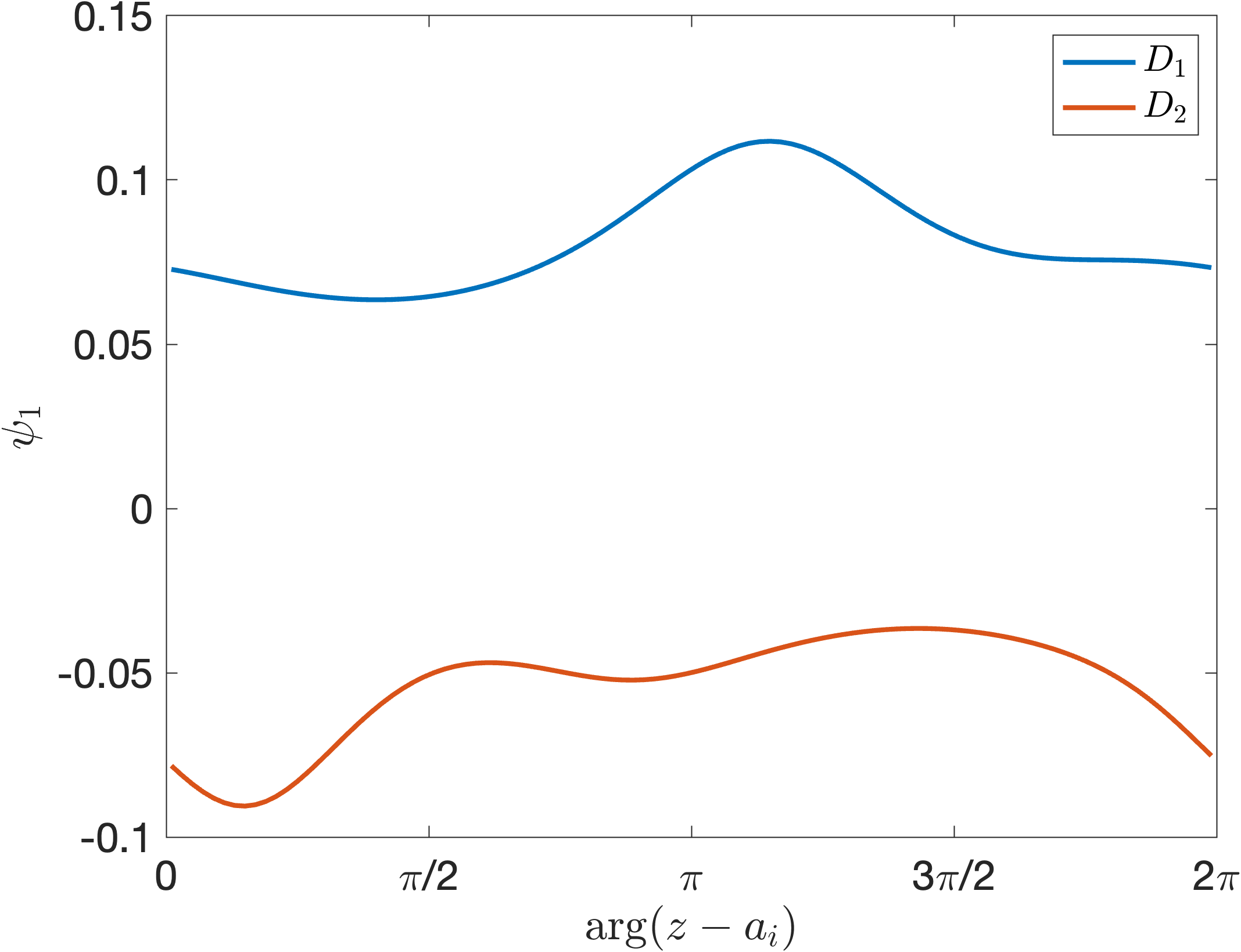
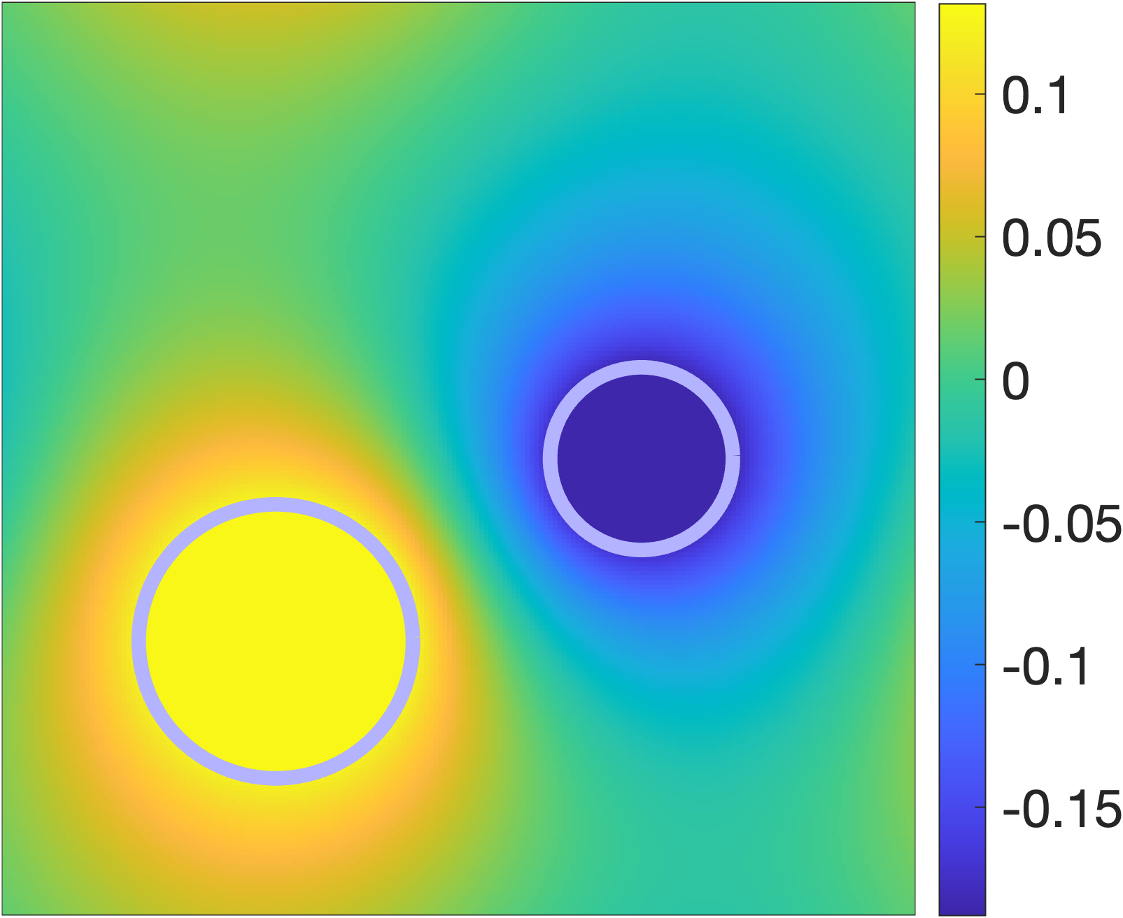
Remark 2.1.

In Lemma 2.2(5), a basis $\{\psi_{k}\}_{k=1}^{M-1}$ of $N(\mathrm{K}^{*}-\tfrac{1}{2}I)$ corresponds to functions $\mathcal{S}[\psi_{k}]$ that are constant on each hole $D_{j}$. In Fig. 2, for a square torus $\mathbb{T}_{\tau}$ ($\tau=i$) with $M=2$ circular holes, we plot $\psi_{1}$ on $\partial\Omega$ (left) and $\mathcal{S}[\psi_{1}](z)$, $z\in\mathbb{T}_{\tau}$ (right). In this case, $\mathbf{s}_{1}=[-0.1856,0.1290]^{T}$. The holes have centers $a_{1}=0.7+0.5i$ and $a_{2}=0.3+0.3i$ with radii $r_{1}=0.1$ and $r_{2}=0.15$. See Sec. 4 for a discussion on the numerical methods used to generate this figure.

Figure 2: For a square torus with $M=2$ circular holes, we plot $\psi_{1}\in N(\mathrm{K}^{*}-\tfrac{1}{2}I)$  (left) and $\mathcal{S}[\psi_{1}](z)$, $z\in\mathbb{T}_{\tau}$ (right). As proven in Lemma 2.2 (5), $\mathcal{S}[\psi_{1}]$ is constant on each hole; see Remark 2.1.

Lemma 2.3 (Properties of Single-Layer Potential).

Let $\Omega$ satisfy Assumption 1.1. The single-layer potential $\mathcal{S}[\phi]$ given in (7) satisfies the following properties:

1. For $\phi\in C_{0}(\partial\Omega)$, $\mathcal{S}[\phi]$ is doubly-periodic, continuous on $\mathbb{T}_{\tau}$, smooth on $\mathbb{T}_{\tau}\setminus\partial\Omega$, and satisfies $\Delta\mathcal{S}[\phi](z)=0$ for $z\in\mathbb{T}_{\tau}\setminus\partial\Omega$.

2. For $\phi\in C_{0}(\partial\Omega)$,the normal derivative of the single layer potential satisfies the “jump relations”,

   $$\partial_{\nu}\mathcal{S}[\phi](z^{\pm}_{0})=\mathrm{K}^{*}[\phi](z_{0})\pm\tfrac{1}{2}\phi(z_{0}),\qquad z_{0}\in\partial\Omega,$$

   where $\mathrm{K}^{*}$ is defined in (12).

3. $\mathrm{S}\colon C_{0}(\partial\Omega)\to C_{0}(\partial\Omega)$ is a compact linear operator.

3 Layer Potential Methods

In this section, we prove Theorems 1.4–1.6, which establish layer potential representations for the solutions to the Dirichlet BVP (2), Neumann BVP (3), and Steklov EVP (4). Throughout the proofs, we employ the Fredholm alternative [18, Appendix D] and adapt arguments for multiply-connected Euclidean domains: for the Dirichlet BVP, we follow [51, Sec. 29] and [25, Sec. 3.1]; for the Neumann BVP, we refer to [52, Sec. 37, Lemma 2]; and for the Steklov EVP, we utilize [42, Theorem 7.36].

3.1 The Dirichlet BVP and Proof of Theorem 1.4

Lemma 2.2(4) shows that the null space of $\mathrm{K}-\tfrac{1}{2}I$ is trivial for $M=1$ and nontrivial for $M\geq 2$. Accordingly, we introduce the following integral operator to handle both cases simultaneously.

Definition 3.1 (Characteristic operator).

Define the characteristic operator as the linear operator $\mathrm{X}\colon C(\partial\Omega)\to C(\partial\Omega)$ for $M=1$ by $\mathrm{X}[\phi]\equiv 0$, and for $M\geq 2$ by

(27) $$\mathrm{X}[\phi](z_{0}):=\int_{\partial\Omega}\chi(z_{0},\xi)\phi(\xi)\,|d\xi|,\qquad z_{0}\in\partial\Omega,$$

where $\chi(z_{0},\xi)\coloneq\sum_{j=1}^{M-1}\mathbbm{1}_{j}(z_{0})\mathbbm{1}_{j}(\xi)$.

The operator $\mathrm{X}$ integrates $\phi$ only over the boundary component containing $z_{0}$, excluding the $M$th component. The following lemma establishes preliminary properties of the characteristic operator.

Lemma 3.2 (Properties of the Characteristic Operator).

Let $\Omega$ satisfy Assumption 1.1. The characteristic operator in (27) satisfies the following properties:

1. $\mathrm{X}$ is a compact linear operator. For any $\phi\in C(\partial\Omega)$, $\mathrm{X}[\phi]$ is a constant function on each $\partial D_{j}$, for $j=1,2,\ldots,M$, and vanishes on $\partial D_{M}$.

2. $\mathrm{K}+\mathrm{X}-\tfrac{1}{2}I\colon C(\partial\Omega)\to C(\partial\Omega)$ is an injective compact linear operator; consequently, by the Fredholm alternative, it is also surjective.

Lemma 3.2 is used in the proof of Theorem 1.4 and is proven in Appendix A. The injectivity of $\mathrm{K}+\mathrm{X}-\tfrac{1}{2}I$ is established using the properties of the complex double-layer potential in Lemma A.3.

Proof 3.3 (Proof of Theorem 1.4).

Our goal is to express system (13) using $\mathrm{K}+\mathrm{X}-\tfrac{1}{2}I$. By applying Lemma 3.2(2), we establish the existence and uniqueness of the system.

$M=1$. Since $\mathrm{X}\equiv 0$ by Definition 3.1, (13) reduces to $\left(\mathrm{K}-\tfrac{1}{2}I\right)[\phi]=g$ (see Remark 1.1). Therefore, for any $g\in C(\partial\Omega)$, there exists a unique $\phi\in C(\partial\Omega)$ satisfying (13). This proves the theorem for the case $M=1$.

$M\geq 2$. Assume $g\in C(\partial\Omega)$ and fix $\beta_{j}\in D_{j}$. We show that there exist unique $\phi_{A}$ and $A_{j}\in\mathbb{R}$ for $j=1,2,\ldots,M$ that solve the system (13). By Lemma 3.2(2), there exists a unique $\phi^{j}\in C(\partial\Omega)$ corresponding to $g^{j}\in C(\partial\Omega)$ for $j=0,1,\ldots,M$, solving

(28) $$(\mathrm{K}+\mathrm{X}-\tfrac{1}{2}I)[\phi^{j}](z_{0})=g^{j}(z_{0}),\qquad z_{0}\in\partial\Omega,\quad\text{where}$$

$$g^{j}(z_{0})=\begin{cases}g(z_{0})&\text{if}\quad j=0,\\ G(z_{0}-\beta_{j})&\text{if}\quad j=1,2,\ldots,M.\end{cases}$$

First, we show that there exists a unique set $\{A_{j}\}_{j=1}^{M}$ satisfying

(29) $$\sum_{j=1}^{M}A_{j}\mathrm{X}[\phi^{j}](z_{0})=\mathrm{X}[\phi^{0}](z_{0}),\qquad z_{0}\in\partial\Omega\qquad\text{and}\qquad\sum_{j=1}^{M}A_{j}=0.$$

Since $\mathrm{X}[\phi^{j}]$ for $j=0,1,\ldots,M$ are piecewise constant on each $\partial D_{k}$, and vanish on $\partial D_{M}$, we may view (29) as an $M\times M$ linear system. Showing that this system is nonsingular implies the uniqueness of $A_{j}$. To show it is nonsingular, assume $\sum_{j=1}^{M}A_{j}\mathrm{X}[\phi^{j}](z_{0})=0$ on $\partial\Omega$ and $\sum_{j=1}^{M}A_{j}=0$. Substituting the first condition into (28) and applying the Fredholm alternative, we obtain

$$\sum_{j=1}^{M}A_{j}\,G(z_{0}-\beta_{j})\ \in\ R(\mathrm{K}-\tfrac{1}{2}I)\ =\ N(\mathrm{K}^{*}-\tfrac{1}{2}I)^{\perp}.$$

Let $\{\psi_{k}\}_{k=1}^{M-1}$ be the basis for $N(\mathrm{K}^{*}-\tfrac{1}{2}I)$ as in Lemma 2.2(5). By (26),

$$0 =\left\langle\sum_{j=1}^{M}A_{j}\,G(\cdot-\beta_{j}),\psi_{k}\right\rangle=\sum_{j=1}^{M}A_{j}\mathcal{S}[\psi_{k}](\beta_{j})=\sum_{j=1}^{M}A_{j}s_{kj}=\begin{bmatrix}A_{1}\,A_{2}\,\ldots\,A_{M}\end{bmatrix}\mathbf{s_{k}},$$

for each $k=1,2,\ldots,M-1$. In addition to these $M-1$ conditions, $\sum_{j=1}^{M}A_{j}=0$ in (29) provides $[A_{1},\ldots,A_{M}]\mathbf{1}_{M}=0$, where $\mathbf{1}_{M}\in\mathbb{R}^{M}$ is the vector of all ones. Finally, since $\{\mathbf{s}_{1},\mathbf{s}_{2},\ldots,\mathbf{s}_{M-1},\mathbf{1}_{M}\}$ forms a basis for $\mathbb{R}^{M}$ (Lemma 2.2(5)), we conclude that $A_{j}=0$ for all $j=1,2,\ldots,M$.

Next, let

(30) $$\phi_{A}(z_{0}):=\phi^{0}(z_{0})-\sum_{j=1}^{M}A_{j}\phi^{j}(z_{0}),\qquad z_{0}\in\partial\Omega,$$

(31) $$u_{A}(z):=\mathcal{D}[\phi_{A}](z)+\sum_{j=1}^{M}A_{j}G(z-\beta_{j}),\qquad z\in\Omega.$$

Recall that the $\phi^{j}$ are already uniquely determined by (28) and the $A_{j}$ uniquely satisfy (29). Taking the interior limit, we get

$$u_{A}(z^{+}_{0}) =(\mathrm{K}-\tfrac{1}{2}I)[\phi_{A}](z_{0})+\sum_{j=1}^{M}A_{j}G(z_{0}-\beta_{j})$$

$$=g(z_{0})-\left(\mathrm{X}[\phi^{0}](z_{0})-\sum_{j=1}^{M}A_{j}\mathrm{X}[\phi^{j}](z_{0})\right)=g(z_{0}),$$

and conclude that $u_{A}$ is the solution to the Dirichlet BVP.

Finally, the flux across $\partial D_{j}$ for $j=1,2,\ldots,M$ is given by

$$\int_{\partial D_{j}}\partial_{\nu}u(z^{+})\,|dz| =-\int_{D_{j}}\Delta\mathcal{D}[\phi](z)\,dA+\sum_{k=1}^{M}A_{k}\int_{D_{j}}\partial_{\nu}G(z-\beta_{k})\,|dz|$$

$$=A_{j}+\sum_{k=1}^{M}A_{k}\left(-\frac{|D_{j}|}{b}\right)=A_{j}.$$

Here, we used Lemma 2.1 and the condition $\sum_{k=1}^{M}A_{k}=0$.

3.2 The Neumann BVP and Proof of Theorem 1.5

Proof 3.4 (Proof of Theorem 1.5).

Let $u(z)=\mathcal{S}[\phi](z)$ as in (17). Calculating $\partial_{\nu}u(z^{+}_{0})$ by using Lemma 2.3(2), we obtain

$$\mathrm{K}^{*}[\phi](z_{0})+\frac{\phi(z_{0})}{2}=g(z_{0}),\qquad z_{0}\in\partial\Omega.$$

By Lemma 2.2(3) and Lemma 2.2(6), $\mathrm{K}^{*}\colon C_{0}(\partial\Omega)\to C_{0}(\partial\Omega)$ is compact and $\mathrm{K}^{*}+\tfrac{1}{2}I$ is injective (here, $C_{0}(\partial\Omega)$ is a closed subspace of $C(\partial\Omega)$). Hence, by the Fredholm alternative, $\mathrm{K}^{*}+\tfrac{1}{2}I$ is surjective. Therefore, we conclude that for any $g\in C_{0}(\Omega)$, there is a unique $\phi\in C_{0}(\partial\Omega)$ such that $u(z)$ is the solution to the Neumann BVP (3), up to an additive constant. Finally, the flux across $\partial D_{j}$ is given by

$$\int_{\partial D_{j}}\partial_{\nu}u(z^{+})\,|dz| =\int_{\partial D_{j}}\partial_{\nu}\mathcal{S}(z^{+})\,|dz|=\left\langle(\mathrm{K}^{*}+\tfrac{1}{2}I)[\phi],\mathbbm{1}_{j}\right\rangle=\left\langle\phi,(\mathrm{K}+\tfrac{1}{2}I)[\mathbbm{1}_{j}]\right\rangle$$

$$=\left\langle\phi,\frac{\mathbbm{1}_{j}}{2}-\frac{|D_{j}|}{b}\mathbbm{1}+\frac{\mathbbm{1}_{j}}{2}\right\rangle=\int_{\partial D_{j}}\phi(\xi)\,|d\xi|,$$

using Lemma 2.1, Lemma 2.3(2), and the fact that $\phi\in C_{0}(\partial\Omega)$.

3.3 The Steklov EVP and Proof of Theorem 1.6

To prove Theorem 1.6, we use the modified single-layer potential in (9) to find a density $\phi\in C(\partial\Omega)$ instead of $\phi\in C_{0}(\partial\Omega)$. Second, we match the boundary data of $\sigma u(z)$ with $\partial_{\nu}u(z)$. To proceed, we define the Neumann-to-Dirichlet map.

Proposition 1.

The Neumann-to-Dirichlet map, $\Lambda\colon C_{0}(\partial\Omega)\to C_{0}^{1}(\partial\Omega)$, can be expressed in terms of layer potentials as

(32) $$\Lambda\coloneq(I-\mathrm{M})\mathrm{S}\left(\mathrm{K}^{*}+\tfrac{1}{2}I\right)^{-1},$$

which, given Neumann boundary data, outputs zero mean Dirichlet boundary data.

The term $(I-\mathrm{M})$ enforces the Dirichlet data to have zero mean on the boundary. We adopt this convention to ensure the uniqueness of the Dirichlet solution, since Neumann boundary data determines a harmonic function only up to an additive constant.

Proof 3.5 (Proof of Proposition 1).

Let $g\in C_{0}(\partial\Omega)$ be Neumann data. By Theorem 1.5, there exists a unique $\psi\in C_{0}(\partial\Omega)$ satisfying (16). By Theorem 1.5, $\mathcal{S}[\psi]+C$ solves the Neumann BVP (3) with boundary data $g$, for any $C\in\mathbb{R}$. We fix the additive constant by applying $(I-\mathrm{M})$; that is, $C$ is the average value of $-\mathrm{S}[\psi]$ on $\partial\Omega$.

Proof 3.6 (Proof of Theorem 1.6).

Suppose $(\sigma_{k},u_{k})$ is an eigenpair of the Steklov EVP (4) with $k\geq 1$ such that $\sigma_{k}>0$. Applying Proposition 1, there exists a unique $\psi_{k}\in C_{0}(\partial\Omega)$ such that $(I-\mathrm{M})\mathrm{S}[\psi_{k}]$ is a solution to the Neumann BVP with data $\partial_{\nu}u_{k}$. Define $\phi_{k}\in C(\partial\Omega)$ by $\phi_{k}(z_{0})=\psi_{k}(z_{0})-\mathrm{M}\mathrm{S}[\psi_{k}]$ so that $\psi_{k}=(I-\mathrm{M})\phi_{k}$ and $\overline{\phi_{k}}=-\mathrm{M}\mathrm{S}[\psi_{k}]$. By construction,

$$(\mathrm{K}^{*}+\tfrac{1}{2})(I-\mathrm{M})[\phi_{k}]=\partial_{\nu}u_{k}=\sigma_{k}u_{k}=\sigma_{k}(I-\mathrm{M})\mathrm{S}[\psi_{k}]=\sigma_{k}\mathrm{S}_{0}[\phi_{k}],$$

proving the existence of a $\phi_{k}$ such that $(\sigma_{k},\phi_{k})$ satisfies (18).

Conversely, suppose $(\sigma_{k},\phi_{k})$ with $\phi_{k}\in C(\partial\Omega)$ satisfies (18). Define $u_{k}(z)=\mathcal{S}_{0}[\phi_{k}](z),$ which is harmonic on $\Omega$. $\partial_{\nu}u_{k}$ is continuous on $\partial\Omega$, since $\partial_{\nu}u_{k}=(\mathrm{K}^{*}+\tfrac{1}{2}I)(I-\mathrm{M})\phi_{k}$ by Lemma 2.3. Thus, $u_{k}$ solves the Steklov EVP (4) with eigenvalue $\sigma_{k}$.

4 Numerical Experiments

In this section, we present numerical experiments for approximating solutions of the Dirichlet BVP (2), Neumann BVP (3), and Steklov EVP (4). In each of the examples, we consider tori with periods $(1,\tau)$ with $\tau=i$ (square torus) and $\tau=\frac{1}{2}+\frac{\sqrt{3}}{2}i$ (equilateral torus). Our implementation utilizes a standard trapezoid Nyström discretization [31][42, Ch. 12] based on the layer potential methods developed in Theorems 1.4–1.6. All numerical results have been obtained using Matlab direct solvers on fully discretized matrices. We utilize the backslash operator ($\backslash$) for the Dirichlet (13) and Neumann BVPs (16), and the eig function for the Steklov EVP (18). The complete implementation of our computational methods is available on GitHub [40]. The runtime for solving the linear systems to compute the density $\phi$ in Examples 1–5 is between 10 and 100 ms on a 2020 MacBook Pro M1. The runtime for Example 6 is $19.6$ minutes.

4.1 Dirichlet boundary value problem

In the following examples, we solve the Dirichlet BVP (2) on a multiply-connected torus, $\Omega=\mathbb{T}_{\tau}\setminus\cup_{j=1}^{M}\overline{D_{j}}$, by varying the number of holes $M$, the period $\tau$, and the Dirichlet boundary data $g$.

Example 1. Dirichlet BVP with a single ($M=1$) hole. We solve the Dirichlet BVP on tori with a single circular hole, as shown in Fig. 3. Let $D=B(a_{1},r)$ be the disk of radius $r=0.2$ centered at $a_{1}=0.5+0.5i$. The boundary data is $g=-\mathrm{S}[\psi]$ with $\psi(\xi)=\sin\arg(\xi-a_{1})$ for $\xi\in\partial D$. By construction, the exact solution is given by $u_{\text{exact}}(z)=-\mathcal{S}[\psi](z)$ for $z\in\Omega$. Note that the kernel of the single-layer potential exhibits a logarithmic singularity near the boundary. To address this, we utilize a splitting technique similar to those in [42, Sec. 12.3] and [41]. We decompose $G$ into a logarithmically singular part, $-\frac{1}{4\pi}\log(4\sin^{2}((s-t)/2))$, and a remainder that is continuous as $s\to t$. The implementation details are available on GitHub [40].

To approximate the solution, consistent with Theorem 1.4, we use the representation $u(z)=\mathcal{D}[\phi](z)$. We use $N=50$ points to discretize the boundary integral equation (13). The evaluation of the double-layer potential near the boundary $\partial\Omega$ is relatively inaccurate due to discretization error. Therefore, to evaluate the error in the numerical computation, we define $E=\|u-u_{\text{exact}}\|_{L^{\infty}(\gamma)}$, where $\gamma$ is the boundary of an enlarged disk, $\partial B(a_{1},r+0.15)$. With $N=50$ grid points, the errors obtained are $E=1.604\times 10^{-13}$ (square torus) and $E=1.605\times 10^{-13}$ (equilateral torus).

Figure 3: Approximate Dirichlet BVP solutions on a square torus  (left) and an equilateral torus (right) with a single circular hole. See Sec. 4.1, Example 1.

Example 2. Dirichlet BVP with $M=3$ holes. We solve the Dirichlet BVP on tori with $M=3$ circular and “trefoil”-shaped holes; see Fig. 4. Both types of holes are centered at $a_{1}=0.7+0.5i$, $a_{2}=0.3+0.3i$, and $a_{3}=0$ with radius $r=0.1$. The trefoils are parameterized by

(33) $$f(z,r,a_{i})\coloneq r\left(1+0.3\cos\left(3\arg(z-a_{i})\right)\right),\qquad z\in\mathbb{T}_{\tau}.$$

For both the square and equilateral tori, define

$$g(z) =\mathcal{S}[\psi](z)+3G(z-a_{1})-G(z-a_{2})-2G(z-a_{3}),\quad z\in\Omega,$$

$$\text{where}\quad\psi(\xi) =\begin{cases}-10\sin\arg(\xi-a_{1})&\text{if }\xi\in\partial D_{1},\\ 10\sin(3\arg(\xi-a_{2}))&\text{if }\xi\in\partial D_{2},\\ -10\sin\arg(\xi-a_{3})&\text{if }\xi\in\partial D_{3}.\end{cases}$$

Using $g\big|_{\partial\Omega}$ as boundary Dirichlet data, by construction, the exact solution is given by $u_{\text{exact}}(z)=g(z)$ for $z\in\Omega$.

To approximate the solution, we represent the solution as in (14). We use $N_{i}=50$ points per boundary component ($N=150$ total) to discretize the boundary integral equation (13a), plus three additional equations to satisfy the conditions in (13b). Consequently, system (13) is represented by a $153\times 153$ matrix equation. As above, to evaluate the error, we define $E=\|u-u_{\text{exact}}\|_{L^{\infty}(\gamma)}$, where $u_{\text{exact}}$ is calculated on a fine grid with $N=3750$. For the circular holes in Fig. 4, we use $\gamma={\cup_{i=1}^{3}}\partial B(a_{i},r+0.08)$ and obtain $E=2.032\times 10^{-13}$ (left) and $E=2.028\times 10^{-13}$(right). For the trefoil holes in Fig. 4, we use $\gamma$ as in (33) with $r=0.18$ and obtain $E=4.300\times 10^{-8}$ (left) and $E=4.299\times 10^{-8}$ (right).

In the bottom plots of Fig. 4, we plot the convergence of the error for increasing $N=4,10,20,\ldots,250$. These plots illustrate that the numerical methods converge spectrally for both the circular and trefoil-shaped holes. The convergence rate for the trefoil-shaped holes is not significantly degraded from the convergence rate for the circular holes; a linear fit for the slope in the log plot yields $-0.0505$ (trefoils) and $-0.0850$ (circles) for the square torus, and $-0.0506$ (trefoils) and $-0.0850$ (circles) for the equilateral torus. For irregularly shaped holes, our layer potential approach exhibits a better convergence rate than the method of particular solutions (MPS) given in [38]. In particular, the $\log_{2}$ error plot in [38, Fig. 4] shows that MPS requires approximately 500 degrees of freedom (dof) to achieve an error that is approximately $3\times 10^{-6}$ on a square torus with two trefoil-shaped holes. Our method achieves comparable error with $N=120$ dof on a square torus with three trefoil-shaped holes.

In Table 1, we report the values of the fluxes $A_{i}$ for $i=1,2,3$ for both the trefoil and circular holes on the square (left) and equilateral torus (right). For both cases, the accuracy of the flux is lower for the trefoil holes than for the circular holes. Because the contribution to flux from $\mathrm{S}[\psi]$ is zero around each hole, the estimated fluxes are very close to the coefficient of $G(z-a_{i})$ in $g(z)$.

Figure 4: Approximate Dirichlet BVP solutions on the square torus  (left) and equilateral torus  (right) with $M=3$ circular holes (top) and trefoil-shaped holes (center). (bottom) The convergence plots illustrate that the numerical methods converge spectrally for both the three circular holes and the three trefoil-shaped holes on square tori  (left) and equilateral tori  (right). The convergence rates for the two shaped holes are similar, but slightly better for the circles. See Sec. 4.1, Example 2.

	Flux, $A_{i}$,	Flux errors	Flux errors
i	for $D_{i}$	(trefoil)	(circle)
1	3	$6.161\times 10^{-11}$	$4.400\times 10^{-16}$
2	-1	$4.411\times 10^{-11}$	$2.200\times 10^{-16}$
3	-2	$1.057\times 10^{-10}$	$2.200\times 10^{-16}$

	Flux errors	Flux errors
i	(trefoil)	(circle)
1	$7.849\times 10^{-11}$	$1.330\times 10^{-15}$
2	$7.463\times 10^{-11}$	$8.900\times 10^{-16}$
3	$3.860\times 10^{-12}$	$2.220\times 10^{-15}$

Table 1: Errors of fluxes for the square  (left) and equilateral  (right) tori in Example 2 (Dirichlet BVP with $M=3$ holes). See Sec. 4.1 and Fig. 4.

Figure 5: Approximate solutions to the Neumann BVP on the square torus  (left) and the equilateral torus (right) with multiple holes. The boundary $\partial\Omega$ is drawn in purple. Since $\mathcal{S}[\phi]$ is continuous across the boundary, we have also plotted $\mathcal{S}[\phi]$ inside $D$. See Sec. 4.2, Example 3 and Table 2.

4.2 Neumann boundary value problem

Example 3. Neumann BVP with $M=8$ holes. We solve the Neumann BVP on tori with $M=8$ holes; the results are shown in Fig. 5. To generate the holes, we randomly chose each center $a_{i}$ for $i=1,2,\ldots,8$, an oscillation factor $\omega_{i}$ with $3\leq\omega_{i}\leq 7$, and the maximum radius of the hole $r_{i}$ (given in Table 2 (left)). The boundary of the hole $\partial D_{i}$ is parametrized by

(34) $$f(z,r_{i},\omega_{i},a_{i})\coloneq\frac{r_{i}}{r_{i}+1}(1+r_{i}\cos\omega_{i}\arg(z-a_{i})),\qquad z\in\mathbb{T}_{\tau}.$$

The boundary data is chosen as $g(z_{0})=\sum_{i=1}^{8}A_{i}\partial_{\nu}G(z_{0}-a_{i})$ for $z_{0}\in\partial\Omega$, where the value of $A_{i}$ for each hole is reported in Table 2(right). By construction, the exact solution is given by $u_{\text{exact}}(z)=\sum_{i=1}^{8}A_{i}G(z-a_{i})+C$ for $z\in\Omega$ and $C\in\mathbb{R}$ is an arbitrary constant.

To approximate the solution, we represent the solution as in (17). We use $N_{i}=50$ points per boundary component ($N=400$ total) to discretize the boundary integral equation (16). The approximate solutions are plotted in Fig. 5. Since the single-layer potential is continuous across $\partial\Omega$, we plot the solution on the entire $\mathbb{T}_{\tau}$ (the domain $\Omega$ and the removed holes).

We evaluate the error in the numerical computation at the boundary $\partial\Omega$ as $E=\|u-u_{\text{exact}}+C\|_{L^{\infty}(\partial\Omega)}$, where $C$ is chosen so that $u$ and $u_{\text{exact}}$ have the same mean. We compute $C$ by averaging $u-u_{\text{exact}}$ on $250$ randomly chosen points on $\Omega$. As in Example 1, we calculate $\mathrm{S}[\phi]$ by decomposing the kernel $G$ into a logarithmically singular part, $-\frac{1}{4\pi}\log(4\sin^{2}((s-t)/2))$, and a remainder that is continuous as $s\to t$. We compute $E=2.100\times 10^{-7}$ (square torus) and $E=2.100\times 10^{-7}$ (equilateral torus). In Table 2 (right), we report the estimated flux errors, $\left|A_{i}-\int_{\partial D_{i}}\phi(\xi)\,|d\xi|\right|$ for $i=1,2,\ldots,8$; see Theorem 1.5. For both values of $\tau$, the estimated fluxes are very close to the coefficients $A_{i}$ in $u_{\text{exact}}$.

i	$\omega_{i}$	$r_{i}$	$a_{i}$
1	6	0.126	0.720 + 0.353i
2	5	0.081	0.320 + 0.420i
3	3	0.082	0.540 + 0.508i
4	3	0.135	0.749 + 0.704i
5	6	0.118	0.408 + 0.725i
6	5	0.108	0.130 + 0.276i
7	6	0.071	0.133 + 0.907i
8	7	0.071	0.369 + 0.169i

$A_{i}$	Flux Errors	Flux Errors
	$\tau=i$	$\tau=1/2+\sqrt{3}i/{2}$
1	$1.284\times 10^{-10}$	$1.318\times 10^{-10}$
2	$3.720\times 10^{-12}$	$4.510\times 10^{-12}$
3	$2.212\times 10^{-11}$	$2.293\times 10^{-11}$
4	$9.690\times 10^{-12}$	$1.168\times 10^{-11}$
-5	$1.588\times 10^{-11}$	$1.744\times 10^{-11}$
-2	$3.026\times 10^{-11}$	$3.159\times 10^{-11}$
-3	$2.990\times 10^{-12}$	$3.610\times 10^{-12}$
0	$2.985\times 10^{-12}$	$3.599\times 10^{-12}$

Table 2:  (left) For the torus in Example 3 (Neumann BVP with $M=8$ holes), we tabulate oscillations, radii, and centers of each hole $D_{i}$ in (34). (right) Error in fluxes for the square and equilateral tori. See Sec. 4.2, Example 3 and Fig. 5.

4.3 Steklov eigenvalue problem

In the following examples, we solve the Steklov EVP (4) on a multiply-connected torus, $\Omega=\mathbb{T}_{\tau}\setminus\cup_{j=1}^{M}\overline{D_{j}}$, by varying the number of holes $M$ and the period $\tau$. For all examples, we approximate the solution using (19) in Theorem 1.6. In particular, Examples 4 and 5 are compared to those in [38]; since the domain in our problem is half the size of the one in [38], we divide the eigenvalues by two before comparing errors.

To compute the eigenvalues $\sigma_{k}$ and the corresponding density functions $\phi_{k}$, we discretize the boundary integral equation (18). The discretization of the adjoint double-layer potential $\mathrm{K}^{*}$ is performed similarly to $\mathrm{K}$, where the diagonal limit is determined by Lemma 2.2(3). For the modified single-layer potential $\mathrm{S}_{0}=\mathrm{S}(I-\mathrm{M})+\mathrm{M}$, we discretize the operators $\mathrm{S}$, $I$, and $\mathrm{M}$ as $N\times N$ matrices. Following the approach in Example 1, we resolve the logarithmic singularity in $\mathrm{S}$ by splitting the kernel into a singular part and a smooth remainder. Using eig function in MATLAB (specifically [V, D] = eig(A, B)), we solve the generalized EVP. We recall that the first eigenvalue is zero.

Example 4. Steklov EVP with a single ($M=1$) hole. We solve the Steklov EVP on tori with a single circular hole; the results are shown in Fig. 6. Let $D=B(a_{1},r)$ be the disk centered at $a_{1}=0.5+0.5i$ with radius $r=0.2$. This example corresponds to Fig. 4 and Fig. 7 in [38], where the eigenvalues are reported in Tables 1 and 4 of [38], with an accuracy of approximately 50 digits.

Using $N=50$ points to discretize the boundary integral equation (18), we calculate 2nd to 7th eigenpairs $(\sigma_{k},u_{k})$ for $k=2,3,\ldots,7$ using the representation in (19); the eigenfunctions are plotted in Fig. 6.

Figure 6: Steklov eigenfunctions $u_{k}$ of the square torus (top two rows) and equilateral torus (bottom two rows) with a single hole. See Sec. 4.3, Example 4, and Table 3.

In Table 3, we tabulate the estimated 2nd to 7th eigenvalues and their associated errors. The errors are computed as the absolute difference between half of our results and those in [38]; we achieve an accuracy of 13 to 16 digits.

$k$	Estimated $\sigma_{k}$	Error
$2$	$3.217375$	$7.550\times 10^{-15}$
$3$	$3.217375$	$1.510\times 10^{-14}$
$4$	$4.850995$	$1.004\times 10^{-13}$
$5$	$5.153581$	$1.155\times 10^{-13}$
$6$	$7.503050$	$3.508\times 10^{-13}$
$7$	$7.503050$	$3.366\times 10^{-13}$

Estimated $\sigma_{k}$	Error
3.348656	$4.440\times 10^{-15}$
3.348656	$1.780\times 10^{-15}$
4.999789	$1.780\times 10^{-15}$
4.999789	$7.100\times 10^{-15}$
7.443925	$1.865\times 10^{-14}$
7.556497	$3.550\times 10^{-15}$

Table 3: For the Steklov EVP on the square torus  (left) and equilateral torus (right) with a single hole, we tabulate the estimated eigenvalues $\sigma_{k}$ and the errors when compared to the values in [38, App. B]. See Sec. 4.3, Example 4 and Fig. 6.

Example 5: Steklov EVP with $M=2$ holes. We consider the Steklov EVP on tori with $M=2$ circular holes; the results are shown in Fig. 7. Let $D=\bigcup_{i=1}^{M}B(a_{i},r)$, the union of disks centered at $a_{1}=0.6+0.5i$ and $a_{2}=0.4+0.6i$ with radii $r=0.05$.

This example corresponds to Fig. 5 and Fig. 8 of [38], where the eigenvalues are reported in Tables 2 and 5 of [38], which are accurate to approximately 50 digits. We use $N_{i}=50$ ($N=100$ total) points to discretize the boundary integral equation (4). We calculate eigenpairs $(\sigma_{k},u_{k})$ for $k=2,3,\ldots,7$ using the representation in (19). We tabulate the 2nd to 7th eigenvalues $\sigma_{k}$ in Table 4 and plot their corresponding eigenfunctions $u_{k}$ given in (19) in Fig. 7. We achieve an accuracy of 14 to 16 digits.

We consider the flux of the $k$-th eigenfunction through the first hole. Since the $k$-th eigenfunction is determined up to a constant multiple, we normalize it with respect to the $L^{2}(\partial\Omega)$ norm and report the absolute value of the flux, $|A_{1}(k)|=\frac{1}{\|u_{k}\|_{L^{2}(\partial\Omega)}}\left|\int_{\partial D_{1}}\partial_{\nu}u_{k}(\xi)\,|d\xi|\right|.$ In Table 4, we report the absolute value of the flux since there are only two holes and recall that $A_{2}(k)=-A_{1}(k)$.

Figure 7: Steklov eigenfunctions $u_{k}$ of the square torus (top two rows) and equilateral torus (bottom two rows) with $M=2$ holes. See Sec. 4.3, Example 5 and Table 4.

$k$	Error in $\sigma_{k}$	$|A_{1}(k)|$
$2$	$9.800\times 10^{-15}$	$4.796$
$3$	$7.100\times 10^{-15}$	$2.216\times 10^{-14}$
$4$	$7.100\times 10^{-15}$	$0.05758$
$5$	$7.100\times 10^{-15}$	$1.267\times 10^{-14}$
$6$	$3.910\times 10^{-14}$	$3.470$
$7$	$1.070\times 10^{-14}$	$0.01060$

Error in $\sigma_{k}$	$|A_{1}(k)|$
$8.000\times 10^{-15}$	$4.863$
$1.780\times 10^{-14}$	$1.412\times 10^{-14}$
$3.200\times 10^{-14}$	$0.002723$
$1.240\times 10^{-14}$	$1.363\times 10^{-14}$
$5.300\times 10^{-15}$	$3.434$
$1.780\times 10^{-14}$	$2.309\times 10^{-14}$

Table 4: For the Steklov EVP on a square torus  (left) and equilateral torus  (right) with $M=2$ holes, we tabulate the error for $\sigma_{k}$ for $k=2,\ldots,7$ when compared to the values in [38, App. B], along with the fluxes $|A_{1}|=|A_{2}|$ of the associated eigenfunctions. See Sec. 4.3, Example 5 and Fig. 7.

Example 6. Steklov EVP with $M=25$ holes. We solve the Steklov EVP on a square torus with $M=25$ holes; the results are shown in Fig. 8. Following the Neumann BVP setup, for each hole, we randomly choose each center $a_{i}$ for $i=1,2,\ldots,M$, the oscillation factor $\omega_{i}$ with $3\leq\omega_{i}\leq 7$, and the maximum radius of the hole $r_{i}$. The boundary of each hole $\partial D_{i}$ is parametrized by (34).

We use $N_{i}=200$ ($N=50000$ total) grid points per boundary component to discretize the boundary integral equation (18). The eigenfunctions $u_{k}$ in (19), corresponding to $\sigma_{k}$, for $k=2$, $52$, $105$, and $500$, are plotted in Fig. 8. As anticipated, the eigenfunctions $u_{k}$ associated with large values of $\sigma_{k}$ become concentrated near $\partial\Omega$ and exhibit oscillations with a wavelength approximately equal to $\frac{2\pi}{\sigma_{k}}$ [23, 58]. The corresponding eigenvalues are reported in Table 5. We note that an a posteriori error estimate can be used to bound the relative errors in $\sigma_{k}$ by $\|\partial_{\nu}u_{k}-\sigma_{k}u_{k}\|_{L^{2}(\partial\Omega)}$; see [10] and [38, Prop. 4.1]. In Table 5, we report $\|\partial_{\nu}u_{k}-\sigma_{k}u_{k}\|_{L^{\infty}(\partial\Omega)}$, approximated using a finer discretization on the boundary. We estimate that the errors in $\sigma_{k}$ are on the order of $10^{-14}$.

$k$	$\sigma_{k}$	$\|\partial_{\nu}u_{k}-\sigma_{k}u_{k}\|_{L^{\infty}(\partial\Omega)}$
$2$	$0.9989357$	$9.760\times 10^{-15}$
$52$	$19.57834$	$1.960\times 10^{-14}$
$105$	$35.13811$	$1.664\times 10^{-14}$
$500$	$138.0663$	$1.386\times 10^{-14}$

Table 5: For the Steklov EVP on a square torus with 25 holes, we tabulate values of $\sigma_{k}$ and $\|\partial_{\nu}u_{k}-\sigma_{k}u_{k}\|_{L^{\infty}(\partial\Omega)}$ for different values of $k$. See Sec. 4.3 Example 6 and Fig. 8.

Figure 8: Eigenfunctions $u_{k}$ of the Steklov EVP (4) corresponding to $\sigma_{k}$, for $k=2$, $52$, $105$, and $500$, are computed on a square torus with $M=25$ holes. The corresponding eigenvalues are tabulated in Table 5. Each hole is discretized with $N=200$ boundary points, resulting in a total of $5000$ degrees of freedom. Using an a posteriori estimate, the eigenvalue approximations have a relative error less than $10^{-14}$. As anticipated, the eigenfunctions $u_{k}$ corresponding to large $\sigma_{k}$ concentrate near $\partial\Omega$ and oscillate with a wavelength $\approx\frac{2\pi}{\sigma_{k}}$ [23, 58]. See Sec. 4.3, Example 6.

5 Discussion

In this paper, we have developed and analyzed layer potential methods to represent harmonic functions on finitely-connected tori. The layer potentials are expressed in terms of a doubly-periodic and non-harmonic Green’s function $G$ in (5). Extending results for Euclidean domains, we establish in Lemmas 2.3 and 2.2 that the single- and double-layer potential operators are compact linear operators and we derive relevant limiting properties at the boundary. Here, we also show that when the boundary has multiple connected component, the Fredholm operator of the second kind, $\mathrm{K}^{*}-\tfrac{1}{2}I$, possesses a non-trivial null space, for which we construct a basis. In Theorems 1.4, 1.5, and 1.6, we use the layer potentials to represent solutions to the Dirichlet BVP (2), Neumann BVP (3), and Steklov EVP (4), respectively. Finally, we implement the developed methods and demonstrate their accuracy across several numerical examples; see Sec. 4.

There are several interesting extensions of this work. First, our method can be improved by incorporating techniques for close evaluation [4, 21], using fast multipole acceleration to solve linear integral equations [28], and handling less regular boundaries (e.g., boundary with corners) [24, 29, 50]. While we solve the Laplace equation on finite-connected tori here, extending these ideas to the Helmholtz and Stokes equations on finitely-connected tori is a natural next step. In this paper we focus on solving BVPs and EVPs on genus one surfaces; from this perspective, the work extends research on solving the Laplace-Beltrami equation on a multiply-connected sphere [43]. It is interesting to extend layer potential methods to higher genus surfaces; recently, progress has been made in this direction for the method of particular solutions [53]. Finally, as we focus on two-dimensional tori, it is interesting to consider developing layer potential methods to represent harmonic functions on higher-dimensional tori.

Appendix A Proofs of lemmas in Sections 2–3

A.1 Preliminary Estimates

This subsection provides the propositions and lemmas required for the proofs in Secs. 2–3. Specifically, the following proposition summarizes the asymptotic properties of $G(z-\xi)$ and its normal derivatives (e.g., (21) and (22)), which are utilized throughout the proofs of Lemmas 2.1–2.3.

Proposition 2 (Asymptotic properties).

Let $\Omega$ satisfy Assumption 1.1 and $z_{0},\xi\in\partial D_{j}$ be sufficiently close. Define $z=z_{0}\mp h\nu(z_{0})$ with $h=|z-z_{0}|$ ($-$ for $z\in\Omega$ and $+$ for $z\in D_{j}$). Then, the following properties hold:

(35) $$G(z-\xi) =-\frac{1}{2\pi}\log|z-\xi|+c+O(|z-\xi|^{2}),$$

(36) $$\partial_{\nu_{\xi}}G(z-\xi) =\frac{(z-\xi)\circ\nu(\xi)}{2\pi|z-\xi|^{2}}+O(|z-\xi|),$$

(37) $$\partial_{\nu_{z}}G(z-\xi) =-\frac{(z-\xi)\circ\nu(z_{0})}{2\pi|z-\xi|^{2}}+O(|z-\xi|),$$

(38) $$\left|\partial_{\nu_{\xi}}G(z-\xi)-\partial_{\nu_{\xi}}G(z_{0}-\xi)\right| \leq\frac{1}{2\pi}\left[\frac{2h}{h^{2}+|z_{0}-\xi|^{2}}+3L_{1,j}\right]+O(h),$$

where $O(|z-\xi|)$ terms are absolutely convergent, $c=\frac{\log|\vartheta_{1}^{\prime}(0)|}{2\pi}$, and $L_{1,j}$ are constants for each $j=1,\ldots,M$.

Proof A.1.

To obtain (35), we use the Weierstrass sigma expansion:

$$G(z-\xi)=-\frac{1}{2\pi}\log|\sigma(z-\xi)|+c+O(|z-\xi|^{2}),$$

where $c=\frac{\log|\vartheta_{1}^{\prime}(0)|}{2\pi}$. This follows from a well-known identity [13, 48],

$$\sigma(z)=e^{\eta_{1}z^{2}/2}\frac{\vartheta_{1}(z)}{\vartheta_{1}^{\prime}(0)}.$$

Furthermore, using the product definition of $\sigma$, we may approximate

$$\log|\sigma(z-\xi)| =\log|z-\xi|+\log\left|\prod_{\omega\neq 0}\left(1-\frac{z-\xi}{\omega}\right)e^{(z-\xi)/\omega+(z-\xi)^{2}/2\omega^{2}}\right|$$

$$=\log|z-\xi|+O(|z-\xi|^{3}),$$

where the infinite product is absolutely and uniformly convergent for $|z|\leq R$ and has order $O(|z-\xi|^{3})$ (see [16]), from which (35) follows.

To obtain (36)-(37), we use the Laurent series of the Weierstrass zeta [13]:

(39) $$\zeta(z)=\frac{1}{z}-\sum_{n=2}^{\infty}c_{n}z^{2n-1}.$$

The series term $O(|z|)$ is absolutely convergent, from which (36)-(37) follows.

Lastly, to obtain (38), we utilize the $C^{2}$ regularity of $\partial D_{j}$ ([42, Lemma 6.16]): there exist positive constants $L_{1,j},L_{2,j}$ such that for all $z_{0},\xi\in\partial D_{j}$,

(40) $$|(z_{0}-\xi)\circ\nu(\xi)| \leq L_{1,j}|z_{0}-\xi|^{2},\quad|\nu(z_{0})-\nu(\xi)|\leq L_{2,j}|z_{0}-\xi|.$$

For $z_{0},\xi\in\partial D_{j}$ sufficiently close, we choose $h=|z-z_{0}|<1/(2L_{1,j})$. Using (40) and [20, Lemma 3.20], we get

$$|z-\xi|^{2}\geq\frac{1}{2}\left(|z-z_{0}|^{2}+|z_{0}-\xi|^{2}\right)\quad\implies\quad\frac{1}{|z-\xi|^{2}}\leq\frac{2}{|z-z_{0}|^{2}+|z_{0}-\xi|^{2}}.$$

We then compute

$$\left|\partial_{\nu_{\xi}}G(z-\xi)-\partial_{\nu_{\xi}}G(z_{0}-\xi)\right| \leq\frac{1}{2\pi}\left[\left|\frac{(z-\xi)\circ\nu(\xi)}{|z-\xi|^{2}}\right|+\left|\frac{(z_{0}-\xi)\circ\nu(\xi)}{|z_{0}-\xi|^{2}}\right|\right]+O(|z-z_{0}|)$$

$$\leq\frac{1}{2\pi}\left[\frac{2|z-z_{0}|+2L_{1,j}|z_{0}-\xi|^{2}}{|z-z_{0}|+|z_{0}-\xi|^{2}}+L_{1,j}\right]+O(|z-z_{0}|)$$

$$\leq\frac{1}{2\pi}\left[\frac{2|z-z_{0}|}{|z-z_{0}|^{2}+|z_{0}-\xi|^{2}}+3L_{1,j}\right]+O(|z-z_{0}|).$$

Next, we introduce a complex double-layer potential and its properties, which are used to prove Lemmas 2.2(4)–(6) and Lemma 3.2. One can understand this potential as the analogue to the Cauchy integral [42, 51, 54].

Definition A.2 (Complex double-layer potential).

Given $\phi\in C(\partial\Omega)$, we define the complex double-layer potential for $z\in\mathcal{P}_{\tau}\setminus\partial\Omega$ by

(41) $$\mathcal{D}_{f}[\phi](z)\coloneq\int_{\partial\Omega}\frac{\phi(\xi)}{2\pi i}\left[\zeta(z-\xi)-\eta_{1}(z-\xi)\right]|d\xi|-\frac{i}{b}\int_{\partial\Omega}(z-\xi)\phi(\xi)\Re[d\xi],$$

where $\mathcal{P}_{\tau}\subset\mathbb{C}$ is the fundamental parallelogram,

(42) $$\mathcal{P}_{\tau}\coloneq\{x+\tau y\in\mathbb{C}:(x,y)\in[0,1]^{2}\}.$$

Here, $\zeta(z)$ is the Weierstrass zeta function with quasi-period $\eta_{1}\coloneq 2\zeta(1/2)$. The associated boundary operator $\mathrm{K}_{f}\colon C^{2}(\partial\Omega)\to C^{2}(\partial\Omega)$ is defined for $z_{0}\in\partial\Omega$ by

(43) $$\mathrm{K}_{f}[\phi](z_{0})\coloneq\mathrm{p.v.}\int_{\partial\Omega}\frac{\phi(\xi)}{2\pi i}\left[\zeta(z_{0}-\xi)-\eta_{1}(z_{0}-\xi)\right]|d\xi|-\frac{i}{b}\int_{\partial\Omega}(z-\xi)\phi(\xi)\Re[d\xi],$$

where $\mathrm{p.v.}$ denotes the Cauchy principal value.

We note that the last term of $\mathcal{D}_{f}[\phi](z)$ in (41) can be expanded as:

$$-\frac{i}{b}\int_{\partial\Omega}(z-\xi)\phi(\xi)\,\Re[d\xi]=-\frac{iz}{b}\left[\int_{\partial\Omega}\phi(\xi)\,\Re[d\xi]\right]+\frac{i}{b}\left[\int_{\partial\Omega}\xi\phi(\xi)\,\Re[d\xi]\right].$$

Since $\phi\in C(\partial\Omega)$, the integrals in the brackets are well-defined constants in $\mathbb{C}$.

Lemma A.3 (Properties of the Complex Double-Layer Potential).

Let $\Omega$ satisfy Assumption 1.1. The complex double-layer potential (41) satisfies the following:

1. For $\phi\in C(\partial\Omega)$, $\mathcal{D}_{f}[\phi]$ is analytic on $\mathcal{P}_{\tau}\setminus\partial\Omega$; therefore, both $\Re\mathcal{D}_{f}[\phi]$ and $\Im\mathcal{D}_{f}[\phi]$ are harmonic on $P_{\tau}\setminus\partial\Omega$. Notably, $\Re\mathcal{D}_{f}[\phi]=\mathcal{D}[\phi]$ is a function on $\mathbb{T}_{\tau}\setminus\partial\Omega$, whereas $\Im\mathcal{D}_{f}[\phi]$ is not necessarily doubly-periodic.

2. For $\phi\in C(\partial\Omega)$, the complex double layer potential satisfies

   $$\mathcal{D}_{f}[\phi](z_{0}^{\pm})=\mathrm{K}_{f}[\phi](z_{0})\mp\tfrac{1}{2}\phi(z_{0}),\qquad z_{0}\in\partial\Omega.$$

Note that Lemma A.3(2) follows from the Sokhotski-Plemelj formula in [42, Thm. 7.8], since $\zeta(z-\xi)$ admits a Laurent series with leading order $(z-\xi)^{-1}$ [48].

Proof A.4.

(1) Following [54], we express $\mathcal{D}[\phi]$ as the real part of a complex function. Let $\xi=\xi(t)$ parametrizes $\partial\Omega$ with the normal vector $\nu(\xi)=-i\frac{\xi^{\prime}(t)}{|\xi^{\prime}(t)|}$. Then, we have

$$\partial_{\nu_{\xi}}G(z-\xi) =-(G_{x}(z-\xi)+iG_{y}(z-\xi))\circ\nu(\xi)$$

$$=\Re\left[\frac{\xi^{\prime}(t)}{i|\xi^{\prime}(t)|}\left(\frac{1}{2\pi}(\zeta(z-\xi)-\eta_{1}(z-\xi))+\frac{i\Im(z-\xi)}{b}\right)\right].$$

Integrating against $\phi(\xi)$ along $\partial\Omega$ yields

$$\mathcal{D}[\phi](z)=\Re\left[\int_{\partial\Omega}\left(\frac{1}{2\pi i}(\zeta(z-\xi)-\eta_{1}(z-\xi))+\frac{\Im(z-\xi)}{b}\right)\phi(\xi)\,d\xi\right].$$

Note that the first two terms on the right-hand side are analytic, whereas the term $\frac{\Im(z-\xi)}{b}$ is non-analytic. Since the latter is continuous, we apply the Cauchy-Riemann equations to identify its harmonic conjugate:

$$-\int_{\partial\Omega}\frac{\Re(z-\xi)}{b}\phi(\xi)\,\Re\left[d\xi\right]=-\Im\left[\frac{i}{b}\int_{\partial\Omega}(z-\xi)\phi(\xi)\,\Re[d\xi]\right].$$

Considering all the terms, we get $\Re\mathcal{D}_{f}[\phi](z)=\mathcal{D}[\phi](z)$ for $\mathcal{D}_{f}[\phi](z)$ in (41).

(2) The result follows from the Sokhotski-Plemelj formula [42, Thm. 7.8], as $\zeta(z-\xi)$ has a Laurent series (39) with leading order $(z-\xi)^{-1}$. Thus, for $\mathbb{T}_{\tau}\ni z\to z_{0}\in\partial\Omega$,

$$\mathcal{D}_{f}[\phi](z)-\mathrm{K}_{f}[\phi](z_{0})=\frac{1}{2\pi i}\int_{\partial\Omega}\phi(\xi)\left[\frac{1}{z-\xi}-\frac{1}{z_{0}-\xi}\right]\,|d\xi|+O(z-z_{0})\to\mp\frac{\phi(z_{0})}{2}.$$

A.2 Proof of Lemma 2.1

Proof A.5.

We first prove (23). Without loss of generality, fix $j$. We use Green’s formula (cf. [36, Ch. 15.6] ) and (6).

Case $z\in\mathbb{T}_{\tau}\setminus\overline{D_{j}}$:

$$\int_{\partial D_{j}}\partial_{\nu_{\xi}}G(z-\xi)\,|d\xi|=-\int_{D_{j}}\Delta_{\xi}G(z-\xi)\,d\xi=-\frac{|D_{j}|}{b}.$$

Case $z\in D_{j}$: Let $\varepsilon>0$ and $D_{j\varepsilon}=D_{j}\setminus B_{\varepsilon}(z)$ for an open ball $B_{\varepsilon}(z)\subset D_{j}$ (see Fig. 9 (left)). The Green’s formula yields:

$$-\frac{|D_{j\varepsilon}|}{b} =-\int_{D_{j\varepsilon}}\Delta_{\xi}G(z-\xi)\,d\xi=\int_{\partial D_{j}}\partial_{\nu_{\xi}}G(z-\xi)\,|d\xi|+\int_{\partial B_{\varepsilon}(z)}\partial_{\nu_{\xi}}G(z-\xi)\,|d\xi|,$$

and (22) implies

$$\int_{\partial B_{\varepsilon}(z)}\partial_{\nu_{\xi}}G(z-\xi)\,|d\xi| =\int_{\partial B_{\varepsilon}(z)}\frac{(z-\xi)\circ(\xi-z)}{2\pi|z-\xi|^{3}}+O(|z-\xi|)\,|d\xi|=-1+O(\varepsilon^{2}).$$

Letting $\varepsilon\to 0$ yields the desired result.

Case $z\in\partial D_{j}$: Let $\varepsilon>0$ and define (see Fig. 9 (right))

$$\begin{split}&\widetilde{C}_{\varepsilon}\coloneq\partial D_{j\varepsilon}\cap\partial B_{\varepsilon}(z)\,\,\textrm{and}\,\,C_{\varepsilon}\coloneq\{y\in\partial B_{\varepsilon}(z)\colon\nu(z)\circ({y-z})\geq 0\};\end{split}$$

Then, Green’s formula and (22) yields

$${-}\frac{|D_{j\varepsilon}|}{b} ={-}\int_{D_{j\varepsilon}}\Delta_{\xi}G(z-\xi)\,d\xi=\int_{\partial D_{j\varepsilon}\setminus\widetilde{C}_{\varepsilon}}\partial_{\nu_{\xi}}G(z-\xi)\,|d\xi|+\int_{\widetilde{C}_{\varepsilon}}\partial_{\nu_{\xi}}G(z-\xi)\,|d\xi|$$

$$=\int_{\partial D_{j\varepsilon}\setminus\widetilde{C}_{\varepsilon}}\partial_{\nu_{\xi}}G(z-\xi)\,|d\xi|-\frac{1}{2}+O(\varepsilon).$$

For the last equality, we use [20, Prop. 3.19],

$$\int_{\widetilde{C}_{\varepsilon}}|d\xi|=\int_{C_{\varepsilon}}|d\xi|+O(\varepsilon^{2})=\pi\varepsilon+O(\varepsilon^{2}).$$

Again, letting $\varepsilon\to 0$ yields the desired result.

Finally, we use (23) to get (24). We sum over $j$ to obtain (24). For $z\in\Omega$, the sum is $-\sum|D_{j}|/b=-|D|/b$. If $z\in D_{k}$, the $k$-th term contributes an additional $1$, yielding $1-|D|/b$. If $z\in\partial D_{k}$, the $k$-th term contributes $1/2$, yielding $1/2-|D|/b$.

Figure 9: Diagrams for the proof of Lemma 2.1:  (left) $z\in D_{j}$; (right) $z\in\partial D_{j}$.

A.3 Proof of Lemma 2.2

Proof A.6.

We follow the proofs for the analogous statements for double-layer potentials on Euclidean domains, as found in [20, Ch. 3], [42, Ch. 6-7], [51, Ch. 4].
(1) The operator $\mathcal{D}$ is linear, and its periodicity follows from the doubly-periodic kernel $\partial_{\nu_{\xi}}G(z-\xi)$, since $G$ is itself doubly-periodic [48]. By (6), we get

$$\Delta\mathcal{D}[\phi](z)=\int_{\partial\Omega}\phi(\xi)\Delta_{z}\partial_{\nu_{\xi}}G(z-\xi)\,|d\xi|=0,\qquad z\in\mathbb{T}_{\tau}\setminus\partial\Omega.$$

(2) We prove the result for $z_{0}^{+}$; the case for $z_{0}^{-}$ follows similarly. Let $z_{0}\in\partial D_{j}$ and $z\in\Omega$ for some $j=1,2,\ldots,M$. Applying (24), we can write

$$\mathcal{D}[\phi](z)-\mathrm{K}[\phi](z_{0})=\int_{\partial\Omega}[\phi(\xi)-\phi(z_{0})]\left[\partial_{\nu_{\xi}}G(z-\xi)-\partial_{\nu_{\xi}}G(z_{0}-\xi)\right]\,|d\xi|\ -\ \tfrac{1}{2}\phi(z_{0}).$$

The proof is completed by showing that:

(44) $$\lim_{z\to z_{0}}\int_{\partial\Omega}[\phi(\xi)-\phi(z_{0})]\left[\partial_{\nu_{\xi}}G(z-\xi)-\partial_{\nu_{\xi}}G(z_{0}-\xi)\right]\,|d\xi|=0.$$

Proof of (44): For $\varepsilon>0$, decompose the integral in (44) into $(I)+(II)$:

$$(I) =\int_{\partial\Omega\setminus B_{\gamma}(z_{0})}[\phi(\xi)-\phi(z_{0})]\left[\partial_{\nu_{\xi}}G(z-\xi)-\partial_{\nu_{\xi}}G(z_{0}-\xi)\right]\,|d\xi|,$$

$$(II) =\int_{\partial D_{j}\cap B_{\gamma}(z_{0})}[\phi(\xi)-\phi(z_{0})]\left[\partial_{\nu_{\xi}}G(z-\xi)-\partial_{\nu_{\xi}}G(z_{0}-\xi)\right]\,|d\xi|,$$

where $B_{\gamma}(z_{0})$ is a ball of fixed radius $\gamma>0$. We show both $|\text{(I)}|$ and $|\text{(II)}|$ can be made less than $\varepsilon/2$ for $z$ sufficiently close to $z_{0}.$

To bound $|\text{(I)}|$, let $S=\partial\Omega\setminus B_{\gamma}(z_{0})$. Since $S$ is compact, $\partial_{\nu_{\xi}}G(z-\xi)$ is uniformly continuous at $z_{0}$ for $\xi\in S$. Therefore, choosing $z$ close to $z_{0}$ will allow

$$|(I)| \leq\left\|\partial_{\nu_{\xi}}G(z-\xi)-\partial_{\nu_{\xi}}G(z_{0}-\xi)\right\|_{L^{\infty}(S)}\left\|\phi(\xi)-\phi(z_{0})\right\|_{L^{\infty}(S)}\int_{S}|d\xi|$$

$$\leq\frac{\varepsilon}{4\|\phi\|_{L^{\infty}(\partial\Omega)}|\partial\Omega|}2\|\phi\|_{L^{\infty}(\partial\Omega)}|\partial\Omega|\leq\frac{\varepsilon}{2}.$$

To bound $|(II)|$, let $z=z_{0}-h\nu(z_{0})$, with $h=|z-z_{0}|$, and define $\tilde{S}=\partial D_{j}\cap B_{\gamma}(z_{0})$. Since $\mathcal{D}[\phi]$ is continuous in $\Omega$, it suffices to consider $z$ along the normal. From (38),

$$|\text{(II)}| \leq\|\phi(z_{0})-\phi(\xi)\|_{L^{\infty}(\tilde{S})}\left[\frac{1}{2\pi}\int_{\tilde{S}}\frac{2h}{h^{2}+|z_{0}-\xi|^{2}}+3L_{1,j}\,|d\xi|+O(h)\right].$$

We consider terms inside the bracket. For the term containing the integral, we use polar coordinates $r=|z_{0}-\xi|$ [20, Ch. 0] to obtain:

$$\frac{1}{2\pi}\int_{\tilde{S}}\frac{2h}{h^{2}+r^{2}}+3L_{1,j}\,|d\xi|\leq 2\int_{0}^{\gamma}\frac{h}{h^{2}+r^{2}}\,dr+\frac{3L_{1,j}|\partial D_{j}|}{2\pi}\to\pi+\frac{3L_{1,j}|\partial D_{j}|}{2\pi}$$

as $h\to 0$. Consequently, as $z\to z_{0}$, the above expression is bounded by a constant $C$, while the remaining $O(h)$ term can also be made smaller than $C$. Finally, allowing $\|\phi(z_{0})-\phi(\xi)\|_{L^{\infty}(\tilde{S})}<\varepsilon/4C$ ensures $|II|\leq\varepsilon/2$.

(3) We show that $\partial_{\nu_{\xi}}G(z-\xi)$ can be continuously extended as $z\to\xi\in\partial\Omega$, implying that $\mathrm{K}$ is compact [42, Thm. 2.27]. Suppose $z,\xi\in\partial D_{j}$ are parameterized by $z(s)=x(s)+iy(s)$, $\xi=z(t)$ for $s,t\in[0,2\pi)$. Using (22) and [41, Sec. 2], we obtain

$$\lim_{z\to\xi}\partial_{\nu_{\xi}}G(z-\xi)=\lim_{s\to t}-\frac{(z(s)-z(t))\circ iz^{\prime}(t)}{2\pi|z^{\prime}(t)||z(s)-z(t)|^{2}}=\frac{y^{\prime}(t)x^{\prime\prime}(t)-x^{\prime}(t)y^{\prime\prime}(t)}{4\pi|z^{\prime}(t)|^{3}}=-\frac{\kappa(\xi)}{4\pi}.$$

Here, the outer normal vector $\nu(\xi)$ and the signed curvature $\kappa(\xi)$ are given by

$$\nu(\xi)=\frac{y^{\prime}(t)-ix^{\prime}(t)}{|z^{\prime}(t)|}\quad\textrm{and}\quad\kappa(\xi)=\frac{x^{\prime}(t)y^{\prime\prime}(t)-y^{\prime}(t)x^{\prime\prime}(t)}{|z^{\prime}(t)|^{3}}.$$

The compactness of the adjoint $\mathrm{K}^{*}$ follows as well [20, Thm. (0.37)]. We also obtain

$$\lim_{z\to\xi}\partial_{\nu_{z}}G(z-\xi)=\lim_{z\to\xi}\overline{\partial_{\nu_{z}}G(z-\xi)}=-\frac{\kappa(\xi)}{4\pi}.$$

(4) We first show that $\dim N(\mathrm{K}-\tfrac{1}{2}I)\leq M-1$. Suppose $\phi\in N(\mathrm{K}-\tfrac{1}{2}I)$. By Lemma 2.2(1)–(2), $\mathcal{D}[\phi]$ solves the homogeneous Dirichlet BVP on $\Omega$, which, by the maximum principle, implies $\mathcal{D}[\phi]=0$ on $\overline{\Omega}$. In addition, by Lemma A.3(1), $\mathcal{D}_{f}[\phi]$ is analytic on $\mathcal{P}_{\tau}\setminus\overline{D}$ with $\Re\mathcal{D}_{f}[\phi]=\mathcal{D}[\phi]=0$. Thus, the Cauchy–Riemann equations imply $\mathcal{D}_{f}[\phi]\equiv iC$ on $\mathcal{P}_{\tau}\setminus\overline{D}$ for some $C\in\mathbb{R}$, yielding $\mathcal{D}_{f}[\phi](z^{+}_{0})\equiv iC$ for all $z_{0}\in\partial D$. Furthermore, Lemma A.3(2) implies for all $z_{0}\in\partial D$,

$$\mathcal{D}_{f}[\phi](z^{-}_{0})=\frac{\phi(z_{0})}{2}+\mathrm{K}_{f}[\phi](z_{0})=\frac{\phi(z_{0})}{2}+\left[\mathcal{D}_{f}[\phi](z^{+}_{0})+\frac{\phi(z_{0})}{2}\right]=\phi(z_{0})+iC.$$

Since $\mathcal{D}_{f}[\phi]$ is analytic on each $D_{j}$ and its imaginary part is constant, the real part $\phi(z_{0})$ must be constant on each $\partial D_{j}$. i.e., $\phi=\sum_{j=1}^{M}c_{j}\mathbbm{1}_{j}$ for some $c_{j}\in\mathbb{R}$.

We show that if $\phi\equiv c$, then $c=0$, implying that $\dim N(\mathrm{K}-\tfrac{1}{2}I)\leq M-1$. Let $\phi\equiv c\in\mathbb{R}$. Since $\phi\in N(\mathrm{K}-\tfrac{1}{2}I)$, it follows from Lemma 2.1 that

$$(\mathrm{K}-\tfrac{1}{2}I)[\phi](z_{0}) =-c\sum_{j=1}^{M}\frac{|D_{j}|}{b}=0\quad\text{for}\quad z_{0}\in\partial\Omega.$$

Since $\sum_{j=1}^{M}\frac{|D_{j}|}{b}\neq 0$ due to Assumption 1.1, it follows that $c=0\equiv\phi$.

Next, we show that $\dim N(\mathrm{K}-\tfrac{1}{2}I)\geq M-1$ by verifying that $\{\phi_{jM}\}_{j=1}^{M-1}$in (25) forms a basis for $N(\mathrm{K}-\tfrac{1}{2}I)$. The set $\{\phi_{jM}\}_{j=1}^{M-1}$ is linearly independent. Furthermore, using $\mathrm{K}[\mathbbm{1}_{j}]=\frac{\mathbbm{1}_{j}}{2}-\frac{|D_{j}|}{b}\mathbb{}$ from (23), we have

$$(\mathrm{K}-\tfrac{1}{2}I)[\phi_{jM}]=\frac{b}{|D_{j}|}\mathrm{K}[\mathbbm{1}_{j}]-\frac{b}{|D_{M}|}\mathrm{K}[\mathbbm{1}_{M}]-\tfrac{1}{2}\phi_{jM}=\tfrac{1}{2}\phi_{jM}-\tfrac{1}{2}\phi_{jM}=0.$$

Thus, we conclude $\dim N(\mathrm{K}-\tfrac{1}{2}I)=M-1$ and $N(\mathrm{K}-\tfrac{1}{2}I)=\textrm{span}\{\phi_{jM}\}_{j=1}^{M-1}$.

(5) Since $\mathrm{K}$ is a compact linear operator by Lemma 2.2(3), the Fredholm alternative and Lemma 2.2(4) imply $\dim N(\mathrm{K}^{*}-\tfrac{1}{2}I)=M-1.$ Let $\{\psi_{jM}\}_{j=1}^{M-1}$ be a basis of this null space. We show (26). Indeed, by Lemma 2.1, we obtain

$$0=\langle(\mathrm{K}^{*}-\tfrac{1}{2}I)\psi_{j},\mathbbm{1}\rangle=\langle\psi_{j},(\mathrm{K}-\tfrac{1}{2}I)[\mathbbm{1}]\rangle=\frac{-|D|}{b}\int_{\partial\Omega}\psi_{j}(\xi)\,|d\xi|,$$

which implies $\int_{\partial\Omega}\psi_{j}(\xi)\,|d\xi|=0$ for all $j$, given that $-|D|/b\neq 0$. Additionally, Lemma 2.3 (2) implies that $\partial_{\nu}\mathcal{S}[\psi_{j}](z^{-}_{0})$ vanishes for all $j$ for all $z_{0}\in\partial\Omega$. Hence, Lemma 2.3 (1) implies that $\mathcal{S}[\psi_{j}](z)$ solves a homogeneous Neumann BVP on $D$; thus, (26a) holds. Equation (26b) then follows from the continuity of $S[\psi_{j}]$ on $\overline{D}$.

To show linear independence of $\{\mathbf{s}_{1},\mathbf{s}_{2},\ldots,\mathbf{s}_{M-1},\mathbf{1}\}$, suppose $\sum_{j=1}^{M-1}c_{j}\mathbf{s}_{j}+c_{M}\mathbf{1}=0$. We show that $c_{j}=0$ for all $j=1,2,\ldots,M$. Let

$$u(z)=\sum_{j=1}^{M-1}c_{j}\mathcal{S}[\psi_{j}](z)\quad\text{for }z\in\mathbb{T}_{\tau}\,\,\implies\,\,u(z)=-c_{M}\quad\text{on }\overline{D}\,\,(\text{because of ~\eqref{eqn: Spsi span}}).$$

Note that $\Delta u(z)=0$ on $\Omega$ and $u(z)$ is continuous throughout $\mathbb{T}_{\tau}$. Thus, $u(z^{+}_{0})=-c_{M}$ implies $u(z)\equiv-c_{M}$ on $\mathbb{T}_{\tau}.$ Finally, apply Lemma 2.3(2) for all $z_{0}\in\partial\Omega$ to obtain

$$0=\partial_{\nu}u(z^{+}_{0})-\partial_{\nu}u(z^{-}_{0})=\sum_{j=1}^{M-1}c_{j}\left[\partial_{\nu}\mathcal{S}[\psi_{j}](z^{+}_{0})-\partial_{\nu}\mathcal{S}[\psi_{j}](z^{-}_{0})\right]=\sum_{j=1}^{M-1}c_{j}\psi_{j}(z_{0}).$$

However, $\{\psi_{j}\}_{j=1}^{M-1}$ forms a basis of $N(\mathrm{K}^{*}-\tfrac{1}{2}I)$, implying $c_{j}=0$ for all $j=1,2,\ldots,M$.

(6) We show that $\dim N(\mathrm{K}^{*}+\tfrac{1}{2}I)=0$, which implies $\dim N(\mathrm{K}+\tfrac{1}{2}I)=0$ from the Fredholm alternative. Let $\phi\in N(\mathrm{K}^{*}+\tfrac{1}{2}I)$. By Lemma 2.1,

$$0=\langle(\mathrm{K}^{*}+\tfrac{1}{2}I)[\phi],\mathbbm{1}\rangle=\langle\phi,(\mathrm{K}+\tfrac{1}{2}I)[\mathbbm{1}]\rangle=\left(1-\frac{|D|}{b}\right)\int_{\partial\Omega}\phi(\xi)\,|d\xi|.$$

Since $|D|<b$ (the area of the holes, $|D|=\sum_{j=1}^{M}|D_{j}|$, is less than the area of the torus, $|\mathbb{T}_{\tau}|=b$), we have $\int_{\partial\Omega}\phi(\xi)\,|d\xi|=0$. By Lemma 2.3(1)–(2), $\mathcal{S}[\phi]$ solves the homogeneous Neumann BVP on $\Omega$, implying $\mathcal{S}[\phi]\equiv C$ on $\overline{\Omega}$, for some $C\in\mathbb{R}$. In addition, by continuity (Lemma 2.3(1)) and the maximum principle, $\mathcal{S}[\phi]\equiv C$ on each $\overline{D}_{j}$ for $j=1,2,\ldots,M$. Finally, the jump relation (Lemma 2.3(2)) yields

$$0=\partial_{\nu}\mathcal{S}[\phi](z^{+}_{0})-\partial_{\nu}\mathcal{S}[\phi](z^{-}_{0})=\phi(z_{0}),\quad\forall z_{0}\in\partial\Omega.$$

Thus, we conclude that $\dim N(\mathrm{K}^{*}+\tfrac{1}{2}I)=0$.

A.4 Proof of Lemma 2.3

Proof A.7.

We follow proofs for the analogous statements for single-layer potentials on Euclidean domains, as found in [20, 42, 41, 54].
(1) The operator $\mathcal{S}$ is linear and inherits doubly-periodic property from its kernel $G(z-\xi)$ [48]. For $\phi\in C_{0}(\partial\Omega)$, a direct calculation yields

$$\Delta\mathcal{S}[\phi](z)=\int_{\partial\Omega}\phi(\xi)\Delta G(z-\xi)\,|d\xi|=\frac{1}{b}\int_{\partial\Omega}\phi(\xi)\,|d\xi|=0,\quad z\in\mathbb{T}_{\tau}\setminus\partial\Omega.$$

To establish continuity on $\mathbb{T}_{\tau}$, it is sufficient to show continuity at $\partial\Omega$, following the argument in [20, Prop. 3.25]. For $z_{0}\in\partial\Omega$ and $\varepsilon>0$, fix $\gamma>0$. For $z\in B_{\gamma}(z_{0})$,

$$|\mathcal{S}[\phi](z)-\mathrm{S}[\phi](z_{0})|\leq \|\phi\|_{L^{\infty}(\partial\Omega)}\int_{\partial\Omega\setminus B_{\gamma}(z_{0})}|G(z_{0}-\xi)-G(z-\xi)|\,|d\xi|$$

$$+\|\phi\|_{L^{\infty}(\partial\Omega)}\int_{\partial\Omega\cap B_{\gamma}(z_{0})}|G(z-\xi)-G(z_{0}-\xi)|\,|d\xi|.$$

The first integral can be bounded by $\varepsilon/(2\|\phi\|_{L^{\infty}(\partial\Omega)})$ for $z$ close to $z_{0}$ due to the uniform continuity of $G$ away from the singularity. For the second term, letting $S=\partial\Omega\cap B_{\gamma}(z_{0})$ and using (35), we simplify

$$\int_{S}|G(z-\xi)-G(z_{0}-\xi)|\,|d\xi| \leq\int_{S}\frac{\log|z-\xi|^{-1}+\log|z_{0}-\xi|^{-1}}{2\pi}\,|d\xi|+O(|z-z_{0}|^{2}).$$

As $z\to z_{0}$, $O(|z-z_{0}|^{2})$ can be made less than $\varepsilon/(4\|\phi\|_{L^{\infty}(\partial\Omega)})$. Evaluated in polar coordinates, the log-integrals are $O(-\gamma\log\gamma)$, which can be made less than $\varepsilon/(4\|\phi\|_{L^{\infty}(\partial\Omega)})$ given that $\gamma$ is fixed small enough. Combined, these estimates ensure $|\mathcal{S}[\phi](z)-\mathrm{S}[\phi](z_{0})|\leq\varepsilon$, establishing continuity at the boundary.

(2) We prove the result for $z_{0}^{+}$, following  [20, Thm. 3.28]; the case for $z_{0}^{-}$ follows similarly. Let $z_{0}\in\partial D_{j}$ and fix $\gamma>0$ small so that for $z\in B_{\gamma}(z_{0})\cap\Omega$, we may express $z=z_{0}-h\nu(z_{0})$. Note that $\mathrm{K}^{*}[\phi](z)$ is continuous on $\partial\Omega$ due to Lemma 2.2(3), so it suffices to show that

$$\lim_{h\to 0}\int_{\partial\Omega}\phi(\xi)\left[J(z,\xi)-J(z_{0},\xi)\right]\,|d\xi|=0,\,\,\text{for}\,\,J(z,\xi):=\partial_{\nu_{z}}G(z-\xi)+\partial_{\nu_{\xi}}G(z-\xi).$$

Here, we evaluate the above integral at $z_{0}$ in the sense of $\mathrm{p.v.}$ Applying Lemma 2.2(2) leads to

$$\partial_{\nu}\mathcal{S}[\phi](z_{0}^{+}) =\lim_{h\to 0}\int_{\partial\Omega}\phi(\xi)\left[J(z_{0},\xi)-\partial_{\nu_{\xi}}G(z-\xi)\right]\,|d\xi|=\tfrac{1}{2}\phi(z_{0})+\mathrm{K}^{*}[\phi](z_{0}).$$

Proof of the claim: Let $\varepsilon>0$. We split the integral into $S=\partial\Omega\setminus B_{\gamma}(z_{0})$ and $\tilde{S}=\partial D_{j}\cap B_{\gamma}(z_{0})$ and show that $|(\text{I})|,|\text{(II)}\leq\varepsilon/2$:

$$\text{(I)}+\text{(II)}=\int_{S}\phi(\xi)\left[J(z,\xi)-J(z_{0},\xi)\right]\,|d\xi|+\int_{\tilde{S}}\phi(\xi)\left[J(z,\xi)-J(z_{0},\xi)\right]\,|d\xi|.$$

To bound $|(I)|$, since $J$ is uniformly continuous away from the singularity, choosing $z$ sufficiently close to $z_{0}$ ensures $\|J(z,\xi)-J(z_{0},\xi)\|_{L^{\infty}(S)}\leq\varepsilon/(2\|\phi\|_{L^{\infty(\partial\Omega)}}|\partial\Omega|)$.

Next, to bound $|\text{(II)}|$, we use approximations (36) and (37) to obtain

$$J(z,\xi)=-\frac{(z-\xi)\circ[\nu(z_{0})-\nu(\xi)]}{2\pi|z-\xi|^{2}}+O(|z-\xi|).$$

The same bound is derived for $z_{0}$ by replacing $z$. Therefore, it follows that

$$\left|\int_{\tilde{S}}\phi(\xi)\left[J(z,\xi)-J(z_{0},\xi)\right]\,|d\xi|\right|$$

$$\leq\frac{\|\phi\|_{L^{\infty}(\partial\Omega)}}{2\pi}\int_{\tilde{S}}\left[\left|\frac{(z-\xi)\circ[\nu(z_{0})-\nu(\xi)]}{|z-\xi|^{2}}\right|+\left|\frac{(z_{0}-\xi)\circ[\nu(z_{0})-\nu(\xi)]}{|z_{0}-\xi|^{2}}\right|\,|d\xi|\right]$$

$$+O(|z-z_{0}|),$$

where $O(|z-z_{0}|)$ can be made less than $\varepsilon/4$ by letting $z$ sufficiently close to $z_{0}$. Since $z$ is normal through $z_{0}$, $|z-\xi|\geq\frac{1}{C}|z_{0}-\xi|$ for some constant. By (40), we have

$$\left|\frac{(z-\xi)\circ[\nu(z_{0})-\nu(\xi)]}{|z-\xi|^{2}}\right| \leq\frac{|\nu(z_{0})-\nu(\xi)|}{|z-\xi|}\leq CL_{2,j}$$

$$\left|\frac{(z_{0}-\xi)\circ[\nu(z_{0})-\nu(\xi)]}{|z_{0}-\xi|^{2}}\right| \leq\frac{|\nu(z_{0})-\nu(\xi)|}{|z_{0}-\xi|}\leq L_{2,j},$$

Hence, choosing a sufficiently small $\gamma$ such that $|\tilde{S}|\leq 2\pi\varepsilon/(4\|\phi\|_{L^{\infty}(\partial\Omega)}(1+C)L_{2,j})$ allows $|\text{(II)}|\leq\varepsilon/2$

(3) We show that $\mathrm{S}$ is an integral operator of order zero, implying its compactness [20, Eq. (3.10) and Props. 3.10]. It is evident that $G(z-\xi)$ remains continuous for $z\neq\xi$. While $G(z-\xi)$ is continuous for $z\neq\xi$, for $z$ near $\xi\in\partial\Omega$, (35) implies:

$$G(z-\xi)=-\frac{1}{2\pi}\log|z-\xi|+c+O(|z-\xi|^{2})=A(z,\xi)\log|z-\xi|+B(z,\xi),$$

where $A(z,\xi)=-\frac{1}{2\pi}$ and $B(z,\xi)$ is a bounded remainder containing the constant and higher-order terms.

A.5 Proof of Lemma 3.2

Proof A.8.

(1) We see that $\mathrm{X}$ is linear and compact, as it has finite rank. By definition, $\mathrm{X}$ is a constant function on each component $\partial D_{j}$:

(45) $$\mathrm{X}[\phi](z_{0})=\begin{cases}\int_{\partial D_{j}}\phi(\xi)\,|d\xi|&\text{if }z_{0}\in\partial D_{j}\text{ for }j=1,2,\ldots,M-1,\\ 0&\text{if }z_{0}\in\partial D_{M}.\end{cases}$$

(2) The compactness and linearity of $\mathrm{K}+\mathrm{X}-\tfrac{1}{2}I$ follows from Lemma 3.2(1) and Lemma 2.2(3). Therefore, the Fredholm alternative implies that injectivity ensures the surjectivity. To establish injectivity, let $\phi\in N(\mathrm{K}+\mathrm{X}-\tfrac{1}{2}I)$; we show that $\phi\equiv 0$. Substituting $\phi$ to $\mathrm{K}+\mathrm{X}-\tfrac{1}{2}I$, we obtain

(46) $$\left(\mathrm{K}-\tfrac{1}{2}\right)[\phi]=\sum_{j=1}^{M-1}c_{j}\mathbbm{1}_{j},\quad\text{ with }c_{j}=-\int_{\partial D_{j}}\phi(\xi)\,|d\xi|.$$

We make the following claim:

Claim: $c_{j}=0,\,\forall j=1,2,\ldots,M-1$.

Postponing the proof of the claim, this implies $\phi\in N(\mathrm{K}-I/2)$, allowing us to express $\phi=\sum_{j=1}^{M-1}d_{j}\phi_{jM}$ using the basis in Lemma 2.2(4), (25). In particular, since $c_{j}=0$ for all $j=1,2,\ldots,M-1$ and (46), we obtain

$$0=c_{j}=-\int_{\partial D_{j}}\phi(z_{0})|dz_{0}|=-d_{j}\frac{b|\partial D_{j}|}{|D_{j}|}\implies d_{j}=0.$$

Thus, $\phi\equiv 0$, confirming injectivity.

Proof of the Claim: By Lemma A.3(1), $\mathcal{D}_{f}[\phi]$ is analytic on $\mathcal{P}\setminus\partial\Omega$, allowing us to apply the Cauchy-Riemann equations:

(47) $$-\partial_{\nu}\Im\mathcal{D}_{f}[\phi](z^{+}_{0})=\partial_{\sigma}\Re\mathcal{D}_{f}[\phi](z^{+}_{0})=\partial_{\sigma}\mathcal{D}[\phi](z^{+}_{0})=0,\quad\forall z_{0}\in\partial\Omega.$$

The tangential derivative $\partial_{\sigma}\mathcal{D}[\phi](z^{+}_{0})$ vanishes since $\mathcal{D}[\phi](z^{+}_{0})$ is piecewise constant on $\partial D_{j}$ according to (46). In addition, we know that $\mathcal{D}_{f}[\phi](z)$ is analytic, so $\Im\mathcal{D}_{f}[\phi](z)$ is harmonic. The Green’s formula over the domain $\mathcal{P}\setminus D$ yields

(48) $$\int_{\mathcal{P}\setminus D}|\nabla\Im\mathcal{D}_{f}[\phi](z)|^{2}\,dA=\int_{\partial\mathcal{P}}\Im\mathcal{D}_{f}[\phi](z)\partial_{\nu}\Im\mathcal{D}_{f}[\phi](z)\,|dz|,$$

where the boundary integrals vanish due to (47).

Figure 10: An illustration of notation introduced in the proof of Lemma 3.2(2) for the parallelogram $\mathcal{P}$ defined in (42).

We show the right-hand side of (48) vanishes by splitting and calculating the integral into four parts $\partial P=\bigcup_{i=1}^{4}\partial P_{i}$ (see Fig. 10). Although $\Im\mathcal{D}_{f}[\phi](z)$ is not periodic, its normal derivative $\partial_{\nu}\Im\mathcal{D}_{f}[\phi](z)$ is doubly periodic due to $\partial_{\nu}\Im\mathcal{D}_{f}[\phi](z)=-\partial_{\sigma}\mathcal{D}[\phi](z)$. Therefore, we simplify the right hand side of (48) as

$$\int_{\partial P_{1}\cup\partial P_{3}} =-\int_{0}^{1}\partial_{\sigma}\Re\mathcal{D}_{f}[\phi](t)\Im\mathcal{D}_{f}[\phi](t)\,dt+\int_{0}^{1}\partial_{\sigma}\Re\mathcal{D}_{f}[\phi](t+\tau)\Im\mathcal{D}_{f}[\phi](t+\tau)\,dt$$

$$=\int_{0}^{1}\partial_{\sigma}\Re\mathcal{D}_{f}[\phi](t)\left[\Im\mathcal{D}_{f}[\phi](t+\tau)-\Im\mathcal{D}_{f}[\phi](t)\right]\,dt=C_{2}\int_{0}^{1}\partial_{\sigma}\Re\mathcal{D}_{f}[\phi](t)\,dt$$

$$=0,$$

where $C_{2}$ is a constant and $\Re\mathcal{D}_{f}[\phi](1)=\Re\mathcal{D}_{f}[\phi](0)$. A similar calculation shows that $\int_{\partial P_{2}\cup\partial P_{4}}=0$. Therefore, we conclude that the right-hand side of (48) is $0$ so that $\Im\mathcal{D}_{f}[\phi]$ is constant on $\mathcal{P}\setminus D$.

Finally, since $\mathcal{D}_{f}[\phi](z)$ is analytic on $\mathcal{P}\setminus\partial\Omega$, the Cauchy-Riemann equations imply that $\Re\mathcal{D}_{f}[\phi](z)=\mathcal{D}[\phi](z)$ is constant on $\Omega$. By (46), $\mathcal{D}[\phi](z^{+}_{0})=\mathrm{K}[\phi](z_{0})-\frac{\phi(z_{0})}{2}=c_{M}=0$ on $\partial D_{M}$, which implies that $c_{1}=\cdots=c_{M-1}=0$, establishing the claim.

References

• [1] H. Ammari, B. Fitzpatrick, H. Kang, M. Ruiz, S. Yu, and H. Zhang, Mathematical and Computational Methods in Photonics and Phononics, American Mathematical Society, 2018, https://doi.org/10.1090/surv/235.
• [2] S. Axler, Harmonic functions from a complex analysis viewpoint, The American Mathematical Monthly, 93 (1986), p. 246, https://doi.org/10.2307/2323672.
• [3] E. A. Baderko, Parabolic problems and boundary integral equations, Mathematical methods in the applied sciences, 20 (1997), pp. 449–459, https://doi.org/10.1002/(SICI)1099-1476(19970325)20:5<449::AID-MMA818>3.0.CO;2-E.
• [4] A. Barnett, Boundary integral equations for BVPs, and their high-order Nyström quadratures: a tutorial, in CBMS Conference on Fast Direct Solvers, 2014.
• [5] A. Barnett and L. Greengard, A new integral representation for quasi-periodic scattering problems in two dimensions, BIT Numerical Mathematics, 51 (2011), pp. 67–90, https://doi.org/10.1007/s10543-010-0297-x.
• [6] A. H. Barnett, G. R. Marple, S. Veerapaneni, and L. Zhao, A unified integral equation scheme for doubly periodic Laplace and Stokes boundary value problems in two dimensions, Communications on Pure and Applied Mathematics, 71 (2018), p. 2334–2380, https://doi.org/10.1002/cpa.21759.
• [7] A. Barton, Layer potentials for general linear elliptic systems, Electronic Journal of Differential Equations, (2017), pp. 1–23, https://ejde.math.txstate.edu/Volumes/2017/309/barton.pdf.
• [8] W. Bergweiler and A. Eremenko, Green’s function and anti-holomorphic dynamics on a torus, Proceedings of the American Mathematical Society, 144 (2016), pp. 2911–3061, https://doi.org/10.1090/proc/13044.
• [9] C. L. Berman and L. Greengard, A renormalization method for the evaluation of lattice sums, Journal of Mathematical Physics, 35 (1994), pp. 6036–6048, https://doi.org/10.1063/1.530726.
• [10] B. Bogosel, The method of fundamental solutions applied to boundary eigenvalue problems, Journal of Computational and Applied Mathematics, 306 (2016), pp. 265–285, https://doi.org/10.1016/j.cam.2016.04.008.
• [11] J. M. Borwein, M. L. Glasser, R. C. McPhedran, J. G. Wan, and I. J. Zucker, Lattice Sums Then and Now, no. 150, Cambridge University Press, 2013, https://doi.org/10.1017/cbo9781139626804.
• [12] P. Cazeaux and O. Zahm, A fast boundary element method for the solution of periodic many-inclusion problems via hierarchical matrix techniques, ESAIM: Proceedings and Surveys, 48 (2015), p. 156–168, https://doi.org/10.1051/proc/201448006.
• [13] K. Chandrasekharan, Elliptic functions, vol. 281, Springer, 1985, https://doi.org/10.1007/978-3-642-52244-4.
• [14] D. Cioranescu and P. Donato, An Introduction to Homogenization, Oxford University Press, 11 1999, https://doi.org/10.1093/oso/9780198565543.001.0001.
• [15] H. Cohn, Conformal mapping on Riemann surfaces, McGraw-Hill, Inc., 1967.
• [16] A. Daniels, Note on Weierstrass’ methods in the theory of elliptic functions, American Journal of Mathematics, 6 (1883), pp. 177–182, https://doi.org/10.2307/2369218.
• [17] O. Emersleben, Das Darcysche Filtergesetz, Physikalische Zeitschrift, 26 (1925), pp. 601–610.
• [18] L. C. Evans, Partial differential equations, vol. 19, American Mathematical Society, second ed., 2010, https://doi.org/10.1090/gsm/019.
• [19] P. P. Ewald, Die Berechnung optischer und elektrostatischer Gitterpotentiale, Annalen der Physik, 369 (1921), pp. 253–287, https://doi.org/10.1002/andp.19213690304.
• [20] G. B. Folland, Introduction to partial differential equations, Princeton University Press, second ed., 1995, https://doi.org/10.2307/j.ctvzsmfgn.
• [21] S. D. Gedney, On deriving a locally corrected Nyström scheme from a quadrature sampled moment method, IEEE Transactions on Antennas and Propagation, 51 (2003), pp. 2402–2412, https://doi.org/10.1109/TAP.2003.816305.
• [22] S. Gemmrich, N. Nigam, and O. Steinbach, Boundary Integral Equations for the Laplace-Beltrami Operator, Springer Berlin Heidelberg, 2008, pp. 21–37, https://doi.org/10.1007/978-3-540-68850-1_2.
• [23] A. Girouard and I. Polterovich, Spectral geometry of the Steklov problem, Journal of Spectral Theory, 7 (2017), pp. 321–359, https://doi.org/10.4171/JST/164.
• [24] T. Goodwill and M. O’Neil, An interface formulation of the Laplace-Beltrami problem on piecewise smooth surfaces, SIAM Journal on Mathematical Analysis, 55 (2023), pp. 7575–7615, https://doi.org/10.1137/22m1538454.
• [25] A. Greenbaum, L. Greengard, and G. B. McFadden, Laplace’s equation and the Dirichlet-Neumann map in multiply connected domains, Journal of Computational Physics, 105 (1993), pp. 267–278, https://doi.org/10.1006/jcph.1993.1073.
• [26] L. Greengard and M. C. Kropinski, Integral equation methods for Stokes flow in doubly-periodic domains, Journal of Engineering Mathematics, 48 (2004), p. 157–170, https://doi.org/10.1023/b:engi.0000011923.59797.92.
• [27] L. Greengard and M. Moura, On the numerical evaluation of electrostatic fields in composite materials, Acta Numerica, 3 (1994), p. 379–410, https://doi.org/10.1017/s0962492900002464.
• [28] L. Greengard and V. Rokhlin, A fast algorithm for particle simulations, Journal of Computational Physics, 73 (1987), pp. 325–348, https://doi.org/10.1016/0021-9991(87)90140-9.
• [29] P. Grisvard, Elliptic problems in nonsmooth domains, SIAM, 2011.
• [30] C. Hafner, The Generalized Multipole Technique for Computational Electromagnetics, Artech House, 1990.
• [31] S. Hao, A. H. Barnett, P. G. Martinsson, and P. Young, High-order accurate methods for Nyström discretization of integral equations on smooth curves in the plane, Advances in Computational Mathematics, (2014), https://doi.org/10.1007/s10444-013-9306-3.
• [32] H. Hasimoto, On the periodic fundamental solutions of the Stokes equations and their application to viscous flow past a cubic array of spheres, Journal of Fluid Mechanics, 5 (1959), p. 317–328, https://doi.org/10.1017/S0022112059000222.
• [33] H. Hasimoto, Periodic Fundamental Solution of a Two-Dimensional Poisson Equation, Journal of the Physical Society of Japan, 77 (2008), p. 104601, https://doi.org/10.1143/JPSJ.77.104601.
• [34] J. Helsing, An integral equation method for elastostatics of periodic composites, Journal of the Mechanics and Physics of Solids, 43 (1995), p. 815–828, https://doi.org/10.1016/0022-5096(95)00018-e.
• [35] J. Helsing and R. Ojala, On the evaluation of layer potentials close to their sources, Journal of Computational Physics, 227 (2008), pp. 2899–2921, https://doi.org/10.1016/j.jcp.2007.11.024.
• [36] P. Henrici, Applied and computational complex analysis, Volume 3: discrete Fourier analysis, Cauchy integrals, construction of conformal maps, univalent functions, John Wiley & Sons, 1986.
• [37] J. D. Joannopoulos, S. G. Johnson, J. N. Winn, and R. D. Meade, Photonic Crystals: Molding the Flow of Light - Second Edition, Princeton University Press, 2011, https://doi.org/10.2307/j.ctvcm4gz9.
• [38] C.-Y. Kao, B. Osting, and E. Oudet, Harmonic functions on finitely connected tori, SIAM Journal on Numerical Analysis, 61 (2023), pp. 2795–2812, https://doi.org/10.1137/23M1569897.
• [39] D. Kapanadze, G. Mishuris, and E. Pesetskaya, Exact solution to a nonlinear heat conduction problem in doubly periodic 2D composite materials, Archives of Mechanics, (2015).
• [40] B. Kim, BIE_periodic. https://github.com/BohyunKim92/BIE_periodic, 2025.
• [41] R. Kress, Boundary integral equations in time-harmonic acoustic scattering, Mathematical and Computer Modelling, 15 (1991), pp. 229–243, https://doi.org/10.1016/0895-7177(91)90068-i.
• [42] R. Kress, Linear integral equations, Springer, third ed., 2014, https://doi.org/10.1007/978-1-4614-9593-2.
• [43] M. C. A. Kropinski and N. Nigam, Fast integral equation methods for the Laplace-Beltrami equation on the sphere, Advances in Computational Mathematics, 40 (2014), p. 577–596, https://doi.org/10.1007/s10444-013-9319-y.
• [44] P. Kuchment, An overview of periodic elliptic operators, Bulletin of the American Mathematical Society, 53 (2016), p. 343–414, https://doi.org/10.1090/bull/1528.
• [45] P. K. Kundu, I. M. Cohen, and D. R. Dowling, Fluid Mechanics, Academic Press, fifth edition ed., 2012, https://doi.org/10.1016/C2009-0-63410-3.
• [46] N. Kuznetsov, T. Kulczycki, M. Kwaśnicki, A. Nazarov, S. Poborchi, I. Polterovich, and B. Siudeja, The Legacy of Vladimir Andreevich Steklov, Notices of the AMS, 61 (2014), p. 190, https://www.ams.org/notices/201401/rnoti-p9.pdf.
• [47] H. Lamb, Hydrodynamics, University Press, 1895, https://doi.org/10.5962/bhl.title.18729.
• [48] C.-S. Lin and C.-L. Wang, Elliptic functions, Green functions and the mean field equations on tori, Annals of Mathematics, (2010), pp. 911–954, https://doi.org/10.4007/annals.2010.172.911.
• [49] D. Lindbo and A.-K. Tornberg, Spectral accuracy in fast Ewald-based methods for particle simulations, Journal of Computational Physics, 230 (2011), pp. 8744–8761, https://doi.org/10.1016/j.jcp.2011.08.022.
• [50] W. C. H. McLean, Strongly elliptic systems and boundary integral equations, Cambridge university press, 2000.
• [51] S. Mikhlin, Integral Equations, Pergamon, 1957, https://doi.org/10.1016/C2013-0-08209-6.
• [52] S. G. Mikhlin, Linear Integral Equations, Reprint, Dover Publications, 2020.
• [53] M. Nahon and Édouard Oudet, Computation of harmonic functions on higher genus surfaces, 2024, https://doi.org/10.48550/arXiv.2410.06763.
• [54] M. M. S. Nasser, A. H. M. Murid, M. Ismail, and E. M. A. Alejaily, Boundary integral equations with the generalized Neumann kernel for Laplace’s equation in multiply connected regions, Applied Mathematics and Computation, 217 (2011), p. 4710–4727, https://doi.org/10.1016/j.amc.2010.11.027.
• [55] H. Ogata, K. Amano, M. Sugihara, and D. Okano, A fundamental solution method for viscous flow problems with obstacles in a periodic array, Journal of Computational and Applied Mathematics, 152 (2003), pp. 411–425, https://doi.org/10.1016/S0377-0427(02)00720-3.
• [56] Y. Otani and N. Nishimura, A fast multipole boundary integral equation method for periodic boundary value problems in three-dimensional elastostatics and its application to homogenization, International Journal for Multiscale Computational Engineering, 4 (2006), p. 487–500, https://doi.org/10.1615/intjmultcompeng.v4.i4.60.
• [57] E. Oudet, C.-Y. Kao, and B. Osting, Computation of free boundary minimal surfaces via extremal Steklov eigenvalue problems, ESAIM: Control, Optimisation and Calculus of Variations, 27 (2021), p. 34, https://doi.org/10.1051/cocv/2021033.
• [58] I. Polterovich, D. A. Sher, and J. A. Toth, Nodal length of Steklov eigenfunctions on real-analytic Riemannian surfaces, Journal für die reine und angewandte Mathematik, (2019), pp. 17–47.
• [59] C. Pozrikidis, Computation of periodic Green’s functions of Stokes flow, Journal of Engineering Mathematics, 30 (1996), p. 79–96, https://doi.org/10.1007/bf00118824.
• [60] L. N. Trefethen, Series solution of Laplace problems, The ANZIAM Journal, 60 (2018), pp. 1–26, https://doi.org/10.1017/s1446181118000093.
• [61] G. A. L. Van De Vorst, Integral formulation to simulate the viscous sintering of a two-dimensional lattice of periodic unit cells, Journal of Engineering Mathematics, 30 (1996), p. 97–118, https://doi.org/10.1007/bf00118825.
• [62] R. Wegmann and M. M. S. Nasser, The Riemann–Hilbert problem and the generalized Neumann kernel on multiply connected regions, Journal of Computational and Applied Mathematics, 214 (2008), pp. 36–57, https://doi.org/10.1016/j.cam.2007.01.021.