arXiv is now an independent nonprofit! Learn more
License: CC Zero
arXiv:2504.15558v2 [math.ST] 01 Nov 2025

Dynamical mean-field analysis of adaptive Langevin diffusions: Replica-symmetric fixed point and empirical Bayes

Zhou Fan ††thanks: Department of Statistics and Data Science, Yale University    Justin Ko ††thanks: Department of Statistics and Actuarial Science, University of Waterloo    Bruno Loureiro ††thanks: Departement d’Informatique, École Normale Supérieure, PSL & CNRS    Yue M. Lu ††thanks: Departments of Electrical Engineering and Applied Mathematics, Harvard University    Yandi Shen ††thanks: Department of Statistics and Data Science, Carnegie Mellon University
Abstract

In many applications of statistical estimation via sampling, one may wish to sample from a high-dimensional target distribution that is adaptively evolving to the samples already seen. We study an example of such dynamics, given by a Langevin diffusion for posterior sampling in a Bayesian linear regression model with i.i.d. regression design, whose prior continuously adapts to the Langevin trajectory via a maximum marginal-likelihood scheme. Results of dynamical mean-field theory (DMFT) developed in our companion paper establish a precise high-dimensional asymptotic limit for the joint evolution of the prior parameter and law of the Langevin sample. In this work, we carry out an analysis of the equations that describe this DMFT limit, under conditions of approximate time-translation-invariance which include, in particular, settings where the posterior law satisfies a log-Sobolev inequality. In such settings, we show that this adaptive Langevin trajectory converges on a dimension-independent time horizon to an equilibrium state that is characterized by a system of scalar fixed-point equations, and the associated prior parameter converges to a critical point of a replica-symmetric limit for the model free energy. As a by-product of our analyses, we obtain a new dynamical proof that this replica-symmetric limit for the free energy is exact, in models having a possibly misspecified prior and where a log-Sobolev inequality holds for the posterior law.

1 Introduction

Parameter estimation via Monte Carlo sampling is a common paradigm in statistical learning, arising for example in stochastic implementations of Expectation-Maximization estimation in latent variable models [1, 2], and contrastive-divergence [3] and diffusion-based learning [4, 5, 6, 7] of generative models for data. In these applications, one wishes to learn a parameter using Monte Carlo samples from an associated distribution on a high-dimensional space. Monte Carlo methods whose target distribution continuously adapts to the learned parameter are natural for such tasks, and we refer to [8, 9, 10, 11, 12] for several recent proposals of this form.

The goal of our current work is to study the learning dynamics in a particular (classical) instance of this paradigm, namely the estimation of the distribution of regression coefficients in a high-dimensional regression model [13, 14]. We will focus on the linear model

𝐲=𝐗​𝜽∗+𝜺\mathbf{y}=\mathbf{X}\bm{\theta}^{*}+\bm{\varepsilon}

with a latent and high-dimensional coefficient vector 𝜽∗∈ℝd\bm{\theta}^{*}\in\mathbb{R}^{d}, whose coordinates have an unknown “prior” distribution g∗g_{*}. Estimation of this prior distribution is a classical example of empirical Bayes inference [15, 16], and arises ubiquitously in genetic association analyses where g∗g_{*} represents the distribution of genetic effect sizes in linear mixed models for complex traits [17, 18, 19, 20, 21, 22, 23, 24]. Two recent works [25, 10] have established the statistical consistency of nonparametric maximum marginal-likelihood estimators of g∗g_{*} in settings of high-dimensional regression designs 𝐗∈ℝn×d\mathbf{X}\in\mathbb{R}^{n\times d}, as n,d→∞n,d\to\infty. However, direct computation of this maximum marginal-likelihood estimate is intractable for general regression designs, motivating approaches based on approximate posterior inference schemes.

We will investigate in this work a parametric analogue of a learning procedure proposed in [10], modeling the prior distribution via a parametric model g⁡(⋅,α)g(\,\cdot\,,\alpha) and applying an adaptive diffusion to estimate the parameter α∈ℝK\alpha\in\mathbb{R}^{K}. This procedure will take the form of a Langevin diffusion

d​𝜽t=∇𝜽​log​𝖯g⁡(⋅,α^t)​(𝜽t∣𝐗,𝐲)​d​t+2​d​𝐛t\mathrm{d}\bm{\theta}^{t}=\nabla_{\bm{\theta}}\log\mathsf{P}_{g(\cdot,\widehat{\alpha}^{t})}(\bm{\theta}^{t}\mid\mathbf{X},\mathbf{y})\mathrm{d}t+\sqrt{2}\,\mathrm{d}\mathbf{b}^{t} (1)

for sampling from the posterior distribution 𝖯g⁡(⋅,α^t)​(𝜽∣𝐗,𝐲)\mathsf{P}_{g(\cdot,\widehat{\alpha}^{t})}(\bm{\theta}\mid\mathbf{X},\mathbf{y}) of the regression coefficients, under a prior law g⁡(⋅,α^t)g(\,\cdot\,,\widehat{\alpha}^{t}) whose parameter evolves according to a coupled continuous-time dynamics

d​α^t=𝒢⁡(α^t,1d​∑j=1dδθjt)​d​t.\mathrm{d}\widehat{\alpha}^{t}=\mathcal{G}\Big(\widehat{\alpha}^{t},\frac{1}{d}\sum_{j=1}^{d}\delta_{\theta_{j}^{t}}\Big)\mathrm{d}t. (2)

Here 𝒢⁡(⋅)\mathcal{G}(\cdot) is a map that implements gradient-based maximum marginal-likelihood learning of α\alpha via the empirical distribution of coordinates of 𝜽t\bm{\theta}^{t}, and we defer a discussion of this motivation to Section 2. The procedure may be understood as an approximation to an idealized dynamics

d​αt=𝒢⁡(αt,𝖯⁡(θt))​d​t\mathrm{d}\alpha^{t}=\mathcal{G}(\alpha^{t},\mathsf{P}(\theta^{t}))\mathrm{d}t (3)

where 𝖯⁡(θt)\mathsf{P}(\theta^{t}) denotes the average law of the coordinates θ1t,…,θdt\theta_{1}^{t},\ldots,\theta_{d}^{t}. For these idealized dynamics, the analyses of [10] may be adapted to show that the prior parameter αt\alpha^{t} converges to a fixed point of the marginal log-likelihood, under certain conditions for the noise and regression design. Related results have also been shown recently in more general latent variable models in [26, 8, 9, 12], which, in addition, provide convergence guarantees for particle approximations of the McKean-Vlasov type d​αt=𝒢⁡(αt,1d​M​∑j=1d∑m=1Mδθjm,t)​d​t\mathrm{d}\alpha^{t}=\mathcal{G}(\alpha^{t},\frac{1}{dM}\sum_{j=1}^{d}\sum_{m=1}^{M}\delta_{\theta_{j}^{m,t}})\mathrm{d}t, having MM parallel sampling chains {𝜽1,t}t≥0,…,{𝜽M,t}t≥0\{\bm{\theta}^{1,t}\}_{t\geq 0},\ldots,\{\bm{\theta}^{M,t}\}_{t\geq 0} for the latent variable 𝜽∈ℝd\bm{\theta}\in\mathbb{R}^{d}, in the limit M→∞M\to\infty.

The aforementioned results are not fully satisfactory in our context of a high-dimensional regression model, and leave open the following two interesting questions about the original dynamics (1–2):

  1. 1.

    Single chain propagation-of-chaos. In the limit of increasing dimensions d→∞d\to\infty, are the idealized dynamics (3) well-approximated by (2) using just a single Langevin chain {𝜽t}t≥0\{\bm{\theta}^{t}\}_{t\geq 0} in ℝd\mathbb{R}^{d}?

  2. 2.

    Characterization of fixed points. Can the fixed points α^\widehat{\alpha} of (2) be explicitly characterized? Does (2) exhibit dimension-free convergence to these fixed points, and in what settings is the fixed point representing the maximum marginal-likelihood estimator of α\alpha unique?

The purpose of our work is to provide answers to these questions in the context of an i.i.d. regression design. Question 1 is addressed in our companion paper [27], which build upon the recent results of [28, 29] to formalize a dynamical mean-field theory (DMFT) approximation of (2) by (3) over dimension-independent time horizons t∈[0,T]t\in[0,T], for a general class of such adaptive Langevin dynamics procedures. Our current paper addresses Question 2 by carrying out an analysis of the resulting DMFT system, under an assumption of a uniform log-Sobolev inequality for the posterior law.

1.1 Summary of results

Our main results provide an analysis of the DMFT equations that approximate the empirical Bayes Langevin dynamics (1–2) in the high-dimensional limit as n,d→∞n,d\to\infty proportionally. En route to this analysis, we obtain also new results for the DMFT approximation of the standard non-adaptive Langevin diffusion (1) with a fixed prior g⁡(⋅)≡g⁡(⋅,α)g(\cdot)\equiv g(\,\cdot\,,\alpha). We summarize these results as follows:

  1. 1.

    In the setting of a non-adaptive Langevin diffusion, we formalize a condition of approximate time-translation-invariance (TTI) for the DMFT system. We perform an analysis of the dynamical fixed-point equations for the DMFT correlation and response functions under this condition, and show that they recover the static fixed-point equations for the free energy and posterior mean-squared-error predicted by a replica-symmetric ansatz [30, 31].

  2. 2.

    We show that a log-Sobolev inequality (LSI) for the posterior law provides a sufficient condition to guarantee the above approximate-TTI property for the DMFT system, and we discuss several settings of log-concavity, high noise, or large sample size where such an LSI holds. As a consequence, we obtain a new dynamical proof of the validity of the replica-symmetric predictions for the free energy and MSE in the Bayesian linear model with a possibly misspecified prior law, under such an LSI condition.

  3. 3.

    When the LSI holds uniformly over the posterior laws corresponding to the deterministic DMFT trajectory of {αt}t≥0\{\alpha^{t}\}_{t\geq 0}, we show that the empirical Bayes estimate α^t\widehat{\alpha}^{t} converges on a dimension-free time horizon to a critical point α∞\alpha^{\infty} of the replica-symmetric limit for the free energy. This is explicitly characterized by a system of scalar fixed-point equations, and we discuss examples of models where this critical point may or may not be unique.

We present and discuss these results and examples in further detail in Section 2.

1.2 Further related literature

Approximating the dynamical behavior of many degrees-of-freedom by an effective single-particle problem interacting self-consistently with its environment is an old idea in the statistical physics literature. Relevant to our work is the development of this idea in the context of disordered systems, and in particular the study of high-dimensional Langevin dynamics of soft-spin variants of the Sherrington-Kirkpatrick model [32, 33] and the spherical p-spin model [34, 35, 36, 37]. Mathematical proofs of these approximations were first shown for such models in the works of [38, 39, 40] using large deviations techniques, and more recently in generalized linear models close to our setting by [28, 29] using different methods around Approximate Message Passing algorithms and iterative Gaussian conditioning. In recent years, DMFT analyses have been applied to study Langevin dynamics and gradient-based optimization in many statistical models and applications, including Gaussian mixture classification [41], matrix and tensor PCA [42, 43, 44], phase retrieval and generalized linear models [45, 46], and learning in perceptron and neural network models [47, 48, 49, 50, 51, 52, 53, 54, 55]. These analyses have uncovered surprising phenomena about the efficacy of gradient-based methods and relationships to landscape complexity for high-dimensional non-convex problems [42].

Understanding the long-time behavior of DMFT systems, in particular in low-temperature regimes characterized by aging or metastability, has been a primary goal in both the physics and mathematics literature since the original inception of these methods (see [56, 57] and references within for a review). Mathematically rigorous analyses of long-time dynamics have been obtained previously for spherical 2-spin models in [58] and related statistical models in [59, 44] by leveraging the rotational invariance of these models. However, such analyses of DMFT are (to our knowledge) quite rare in more general settings. Our work takes a step towards filling this gap, by providing a rigorous analysis of the DMFT approximation to Langevin dynamics in a more general model without a rotationally invariant prior, in settings where approximate-TTI holds.

As a by-product of our analyses, we obtain a new proof of a replica formula [60] for the free energy and posterior MSE in the Bayesian linear model. This proof is different from several existing proofs of this result [61, 62, 63, 64, 65] and from the Gaussian interpolation methods of Guerra-Talagrand [66, 67], and is based instead on deducing a static fixed-point equation from the dynamical fixed-point equations of DMFT. Our current result is specific to a high-temperature regime where a LSI holds for the posterior law, but it applies to models where the prior law is misspecified [30, 31, 68]. In this misspecified context, the closest mathematical result of which we are aware is [69] which proved the replica-symmetric predictions in a setting where the posterior is log-concave. A complete large deviations analysis of the free energy in a related rank-one matrix estimation model with misspecified prior and noise was carried out in [70], showing that in general the asymptotic free energy is characterized by a Parisi-type variational problem whose solution may not be replica-symmetric. Our results imply for the linear model that this solution must be replica-symmetric under our assumed condition of a LSI for the posterior law.

In the context of adaptive empirical Bayes Langevin dynamics, our results complement the previous analyses of [10] for more general regression designs, and of [8, 12] in general latent variable models. We deduce a dimension-free convergence rate, in contrast to the results of [10] that established convergence (for a nonparametric variant of this algorithm) on a time horizon growing linearly with n,dn,d, and without employing a time-dependent and decaying learning rate as in [12]. Under the additional mean-field structure of our current model, we are able to establish convergence of a single-chain implementation of the empirical Bayes Langevin dynamics using (2), rather than for an idealized dynamics as studied in [10, 12] or for an implementation using MM parallel chains as studied in [8]. We are also able to give an explicit characterization and analysis of the fixed points to which the dynamics of {α^t}t≥0\{\widehat{\alpha}^{t}\}_{t\geq 0} may converge.

Acknowledgments

This research was initiated during the “Huddle on Learning and Inference from Structured Data” at ICTP Trieste in 2023. We’d like to thank the huddle organiers Jean Barbier, Manuel Sáenz, Subhabrata Sen, and Pragya Sur for their hospitality and many helpful discussions. We are very grateful to Andrea Montanari who suggested to us the approach to prove Theorem 2.5. We’d like to thank also Pierfrancesco Urbani, Francesca Mignacco and Emanuele Troiani for useful discussions. Z. Fan was supported in part by NSF DMS–2142476 and a Sloan Research Fellowship. J. Ko was supported in part by the Natural Sciences and Engineering Research Council of Canada (NSERC), the Canada Research Chairs programme, and the Ontario Research Fund [RGPIN-2020-04597, DGECR-2020-00199]. B. Loureiro was supported by the French government, managed by the National Research Agency (ANR), under the France 2030 program with the reference “ANR-23-IACL-0008” and the Choose France - CNRS AI Rising Talents program. Y. M. Lu was supported in part by the Harvard FAS Dean’s Competitive Fund for Promising Scholarship and by a Harvard College Professorship.

Notational conventions

In the context of the posterior law 𝖯g​(𝜽∣𝐗,𝐲)\mathsf{P}_{g}(\bm{\theta}\mid\mathbf{X},\mathbf{y}) for a given prior g⁡(⋅)g(\cdot), we will write

⟨f(𝜽)⟩=𝔼[f(𝜽)∣𝐗,𝐲]\langle f(\bm{\theta})\rangle=\mathbb{E}[f(\bm{\theta})\mid\mathbf{X},\mathbf{y}]

for the posterior expectation conditioning on the “quenched” variables 𝐗,𝐲\mathbf{X},\mathbf{y}. In the context of Langevin dynamics, we will write similarly

⟨f(𝜽t)⟩=𝔼[f(𝜽t)∣𝐗,𝐲]\langle f(\bm{\theta}^{t})\rangle=\mathbb{E}[f(\bm{\theta}^{t})\mid\mathbf{X},\mathbf{y}]

also for an expectation conditioning on 𝐗,𝐲\mathbf{X},\mathbf{y}. In some arguments it is convenient to consider the expectation also conditioned on the initial condition 𝜽0\bm{\theta}^{0}, and we will denote this by

⟨f(𝜽t)⟩𝐱=𝔼[f(𝜽t)∣𝐗,𝐲,𝜽0=𝐱].\langle f(\bm{\theta}^{t})\rangle_{\mathbf{x}}=\mathbb{E}[f(\bm{\theta}^{t})\mid\mathbf{X},\mathbf{y},\,\bm{\theta}^{0}=\mathbf{x}].

We reserve 𝔼\mathbb{E} and ℙ\mathbb{P} for the full expectation and probability also over 𝐗,𝐲,𝜽∗,𝜺\mathbf{X},\mathbf{y},\bm{\theta}^{*},\bm{\varepsilon}.

Constants C,C′,c,c′>0C,C^{\prime},c,c^{\prime}>0 throughout are independent of the dimensions n,dn,d. For any random variable ξ\xi in a complete and separable normed vector space (ℳ,∥⋅∥)(\mathcal{M},\|\cdot\|), we will use 𝖯⁡(ξ)\mathsf{P}(\xi) to denote its law. 𝒫2​(ℳ)\mathcal{P}_{2}(\mathcal{M}) is the space of probability distributions 𝖯\mathsf{P} on (ℳ,∥⋅∥)(\mathcal{M},\|\cdot\|) such that 𝔼ξ∼𝖯​‖ξ‖2<∞\mathbb{E}_{\xi\sim\mathsf{P}}\|\xi\|^{2}<\infty, and W1​(⋅)W_{1}(\cdot) and W2​(⋅)W_{2}(\cdot) denote the Wasserstein-1 and Wasserstein-2 metrics on 𝒫2​(ℳ)\mathcal{P}_{2}(\mathcal{M}).

For f:ℝd→ℝf:\mathbb{R}^{d}\to\mathbb{R}, ∇f∈ℝd\nabla f\in\mathbb{R}^{d} is its gradient, ∇2f∈ℝd×d\nabla^{2}f\in\mathbb{R}^{d\times d} its Hessian, and ∇3f∈ℝd×d×d\nabla^{3}f\in\mathbb{R}^{d\times d\times d} the symmetric tensor of its 3rd3^{\text{rd}}-order partial derivatives. For f:ℝ×ℝK→ℝf:\mathbb{R}\times\mathbb{R}^{K}\to\mathbb{R}, ∂θf⁡(θ,α)\partial_{\theta}f(\theta,\alpha) and ∇αf​(θ,α)\nabla_{\alpha}f(\theta,\alpha) denote its partial derivatives with respect to θ∈ℝ\theta\in\mathbb{R} and α∈ℝK\alpha\in\mathbb{R}^{K}. ∥⋅∥2\|\cdot\|_{2} is the Euclidean norm for vectors and vectorized Euclidean norm for matrices and tensors. Tr⁡M\Tr M and ‖M‖op\|M\|_{\mathrm{op}} are the matrix trace and Euclidean operator norm. C⁡([0,T],ℝd)C([0,T],\mathbb{R}^{d}) is the space of continuous functions f:[0,T]→ℝdf:[0,T]\to\mathbb{R}^{d} equipped with the norm of uniform convergence ‖f‖∞=supt∈[0,T]‖f⁡(t)‖2\|f\|_{\infty}=\sup_{t\in[0,T]}\|f(t)\|_{2}. Ck​(ℝd,ℝm)C^{k}(\mathbb{R}^{d},\mathbb{R}^{m}) is the space of functions f:ℝd→ℝmf:\mathbb{R}^{d}\to\mathbb{R}^{m} that are kk-times continuously-differentiable. For two probability densities p,qp,q on ℝd\mathbb{R}^{d}, DKL(p∥q)=∫q(logq−logp)\DKL(p\|q)=\int q(\log q-\log p) is the Kullback-Leibler divergence. For a scalar random variable XX, Var⁡X=𝔼​X2−(𝔼​X)2\Var X=\mathbb{E}X^{2}-(\mathbb{E}X)^{2} and Ent⁡X=𝔼​X​log⁡X−𝔼​X​log⁡𝔼​X\Ent X=\mathbb{E}X\log X-\mathbb{E}X\log\mathbb{E}X. For a random vector X∈ℝkX\in\mathbb{R}^{k}, Cov⁡X=𝔼​X​X⊤−(𝔼​X)​(𝔼​X)⊤∈ℝk×k\Cov X=\mathbb{E}XX^{\top}-(\mathbb{E}X)(\mathbb{E}X)^{\top}\in\mathbb{R}^{k\times k}.

2 Model and main results

2.1 Bayesian linear model and adaptive Langevin dynamics

We study a linear model

𝐲=𝐗​𝜽∗+𝜺∈ℝn\mathbf{y}=\mathbf{X}\bm{\theta}^{*}+\bm{\varepsilon}\in\mathbb{R}^{n} (4)

with random effects 𝜽∗∈ℝd\bm{\theta}^{*}\in\mathbb{R}^{d}. Modeling θ1∗,…,θd∗​∼i​i​d​g\theta_{1}^{*},\ldots,\theta_{d}^{*}\overset{iid}{\sim}g for a prior density g⁡(⋅)g(\cdot) on the real line and modeling 𝜺∼𝒩⁡(0,σ2​𝐈)\bm{\varepsilon}\sim\mathcal{N}(0,\sigma^{2}\mathbf{I}) as Gaussian noise, Bayesian inference for 𝜽∗\bm{\theta}^{*} is based upon the posterior density

𝖯g​(𝜽∣𝐗,𝐲)=1𝖯g​(𝐲∣𝐗)​1(2​π​σ2)n/2​exp⁡(−12​σ2​‖𝐲−𝐗​𝜽‖22)​∏j=1dg⁡(θj).\mathsf{P}_{g}(\bm{\theta}\mid\mathbf{X},\mathbf{y})=\frac{1}{\mathsf{P}_{g}(\mathbf{y}\mid\mathbf{X})}\frac{1}{(2\pi\sigma^{2})^{n/2}}\exp\bigg({-}\frac{1}{2\sigma^{2}}\|\mathbf{y}-\mathbf{X}\bm{\theta}\|_{2}^{2}\bigg)\prod_{j=1}^{d}g(\theta_{j}). (5)

Here 𝖯g​(𝐲∣𝐗)\mathsf{P}_{g}(\mathbf{y}\mid\mathbf{X}) is the marginal likelihood of 𝐲\mathbf{y} (i.e. model evidence or partition function), given by

𝖯g​(𝐲∣𝐗)=∫1(2​π​σ2)n/2​exp⁡(−12​σ2​‖𝐲−𝐗​𝜽‖22)​∏j=1dg⁡(θj)​d​θj.\mathsf{P}_{g}(\mathbf{y}\mid\mathbf{X})=\int\frac{1}{(2\pi\sigma^{2})^{n/2}}\exp\bigg({-}\frac{1}{2\sigma^{2}}\|\mathbf{y}-\mathbf{X}\bm{\theta}\|_{2}^{2}\bigg)\prod_{j=1}^{d}g(\theta_{j})\mathrm{d}\theta_{j}. (6)

We will study (overdamped) Langevin dynamics for sampling from the posterior density (5) in two settings, the first in which the prior law g⁡(⋅)g(\cdot) is fixed but may be misspecified, and the second in which this prior law may adapt to the Langevin trajectory to implement empirical Bayes learning from the observed data (𝐗,𝐲)(\mathbf{X},\mathbf{y}). In the former setting, we consider the Langevin dynamics

d​𝜽t=∇𝜽(−12​σ2​‖𝐲−𝐗​𝜽t‖22+∑j=1dlog⁡g⁡(θjt))​d​t+2​d​𝐛t\mathrm{d}\bm{\theta}^{t}=\nabla_{\bm{\theta}}\bigg({-}\frac{1}{2\sigma^{2}}\|\mathbf{y}-\mathbf{X}\bm{\theta}^{t}\|_{2}^{2}+\sum_{j=1}^{d}\log g(\theta_{j}^{t})\bigg)\mathrm{d}t+\sqrt{2}\,\mathrm{d}\mathbf{b}^{t} (7)

where {𝐛t}t≥0\{\mathbf{b}^{t}\}_{t\geq 0} is a standard Brownian motion on ℝd\mathbb{R}^{d}. In the latter setting, we will model the prior via a parametric model

{g⁡(⋅,α):α∈ℝK}\big\{g(\;\cdot\;,\alpha):\alpha\in\mathbb{R}^{K}\big\} (8)

and consider the empirical Bayes Langevin dynamics

d​𝜽t\displaystyle\mathrm{d}\bm{\theta}^{t} =∇𝜽(−12​σ2​‖𝐲−𝐗​𝜽t‖22+∑j=1dlog⁡g⁡(θjt,α^t))​d​t+2​d​𝐛t\displaystyle=\nabla_{\bm{\theta}}\bigg({-}\frac{1}{2\sigma^{2}}\|\mathbf{y}-\mathbf{X}\bm{\theta}^{t}\|_{2}^{2}+\sum_{j=1}^{d}\log g(\theta_{j}^{t},\widehat{\alpha}^{t})\bigg)\mathrm{d}t+\sqrt{2}\,\mathrm{d}\mathbf{b}^{t} (9)
d​α^t\displaystyle\mathrm{d}\widehat{\alpha}^{t} =∇α(1d​∑j=1dlog⁡g⁡(θjt,α^t)−R⁡(α^t))​d​t.\displaystyle=\nabla_{\alpha}\bigg(\frac{1}{d}\sum_{j=1}^{d}\log g(\theta_{j}^{t},\widehat{\alpha}^{t})-R(\widehat{\alpha}^{t})\bigg)\mathrm{d}t. (10)

The equation (10) describes a continuous-time evolution of the prior parameter α∈ℝK\alpha\in\mathbb{R}^{K} that is coupled to the Langevin diffusion (9) of the posterior sample, and R:ℝK→ℝR:\mathbb{R}^{K}\to\mathbb{R} is a possible smooth regularizer. (In this work, we will be interested mostly in the behavior of these dynamics when R⁡(α)≡0R(\alpha)\equiv 0, and we introduce R⁡(α)R(\alpha) for theoretical purposes to confine the dynamics of α^t\widehat{\alpha}^{t} in certain examples.)

To motivate the dynamics (9–10) as a procedure that implements maximum marginal-likelihood learning of α∈ℝK\alpha\in\mathbb{R}^{K}, we may consider the free energy (i.e. negative marginal log-likelihood)

F^​(α)=−1d​log⁡𝖯g⁡(⋅,α)​(𝐲∣𝐗)\widehat{F}(\alpha)={-}\frac{1}{d}\log\mathsf{P}_{g(\cdot,\alpha)}(\mathbf{y}\mid\mathbf{X}) (11)

as a function of the prior parameter α∈ℝK\alpha\in\mathbb{R}^{K}. By the Gibbs variational principle (c.f. [71, Proposition 4.7]),

F^​(α)=infq∈𝒫∗​(ℝd)V⁡(q,α)\widehat{F}(\alpha)=\inf_{q\in\mathcal{P}_{*}(\mathbb{R}^{d})}V(q,\alpha) (12)

where 𝒫∗​(ℝd)\mathcal{P}_{*}(\mathbb{R}^{d}) is the space of all probability densities on ℝd\mathbb{R}^{d}, and

V⁡(q,α)=1d​∫(12​σ2​‖𝐲−𝐗​𝜽‖2−∑j=1dlog⁡g⁡(θj,α)+log⁡q⁡(𝜽))​q​(𝜽)​𝑑𝜽+n2​d​log​2​π​σ2V(q,\alpha)=\frac{1}{d}\int\Big(\frac{1}{2\sigma^{2}}\|\mathbf{y}-\mathbf{X}\bm{\theta}\|^{2}-\sum_{j=1}^{d}\log g(\theta_{j},\alpha)+\log q(\bm{\theta})\Big)q(\bm{\theta})\mathrm{d}\bm{\theta}+\frac{n}{2d}\log 2\pi\sigma^{2} (13)

is the Gibbs free energy corresponding to the prior g⁡(⋅)=g⁡(⋅,α)g(\cdot)=g(\,\cdot\,,\alpha). We propose to implement maximum-likelihood learning of α∈ℝK\alpha\in\mathbb{R}^{K} by minimizing the regularized Gibbs free energy V⁡(q,α)+R⁡(α)V(q,\alpha)+R(\alpha) jointly over (q,α)(q,\alpha), via a gradient flow in the Wasserstein-2 geometry for q∈𝒫∗​(ℝd)q\in\mathcal{P}_{*}(\mathbb{R}^{d}) and the standard Euclidean geometry for α∈ℝK\alpha\in\mathbb{R}^{K}. The resulting gradient flow equations take the form

dd​t​qt\displaystyle\frac{\mathrm{d}}{\mathrm{d}t}q_{t} =−d⋅gradqW2V(qt,αt):=∇𝜽⋅[qt(𝜽)∇𝜽(12​σ2∥𝐲−𝐗𝜽∥22−∑j=1dlogg(θj,αt))]+Tr∇𝜽2qt(𝜽),\displaystyle={-}d\cdot\mathrm{grad}_{q}^{W_{2}}V(q_{t},\alpha^{t}):=\nabla_{\bm{\theta}}\cdot\bigg[q_{t}(\bm{\theta})\nabla_{\bm{\theta}}\bigg(\frac{1}{2\sigma^{2}}\|\mathbf{y}-\mathbf{X}\bm{\theta}\|_{2}^{2}-\sum_{j=1}^{d}\log g(\theta_{j},\alpha^{t})\bigg)\bigg]+\Tr\nabla_{\bm{\theta}}^{2}q_{t}(\bm{\theta}), (14)
dd​t​αt\displaystyle\frac{\mathrm{d}}{\mathrm{d}t}\alpha^{t} =−∇α[V⁡(qt,αt)+R⁡(αt)]=∇α(∫1d​∑j=1dlog⁡g⁡(θj,αt)​qt​(𝜽)​𝑑𝜽−R⁡(αt)).\displaystyle={-}\nabla_{\alpha}[V(q_{t},\alpha^{t})+R(\alpha^{t})]=\nabla_{\alpha}\bigg(\int\frac{1}{d}\sum_{j=1}^{d}\log g(\theta_{j},\alpha^{t})\,q_{t}(\bm{\theta})\mathrm{d}\bm{\theta}-R(\alpha^{t})\bigg). (15)

In (14), we identify gradqW2​V​(q,α)\mathrm{grad}_{q}^{W_{2}}V(q,\alpha) with the Fokker-Planck equation for the density evolution of 𝜽t\bm{\theta}^{t} under the Langevin diffusion (7) with prior law g⁡(⋅)=g⁡(⋅,α)g(\cdot)=g(\,\cdot\,,\alpha), via its variational interpretation put forth in [72]. Then (9–10) may be understood as a particle implementation of (14–15) that uses a single Langevin trajectory {𝜽t}t≥0\{\bm{\theta}^{t}\}_{t\geq 0} to simulate the dynamics of qtq_{t} in (14), and that uses the empirical distribution 1d​∑j=1dδθjt\frac{1}{d}\sum_{j=1}^{d}\delta_{\theta_{j}^{t}} to approximate the expectation over 𝜽∼qt\bm{\theta}\sim q_{t} in the dynamics of αt\alpha^{t} in (15). An algorithm similar to (9–10) was introduced in [10], with some additional reparametrization ideas to allow for nonparametric modeling of the prior g⁡(⋅)g(\cdot). Here, to simplify technical considerations, we restrict our study to parametric prior models of the form (8).

2.2 DMFT equations

The empirical Bayes Langevin diffusion (9–10) is an example of a general class of adaptive Langevin diffusions that we study in our companion work [27]. In particular, the gradient equation (10) for α^t\widehat{\alpha}^{t} is a function of the empirical distribution of coordinates 𝜽t\bm{\theta}^{t},

d​α^t=𝒢⁡(α^t,1d​∑j=1dδθjt)​d​t\mathrm{d}\widehat{\alpha}^{t}=\mathcal{G}\Big(\widehat{\alpha}^{t},\frac{1}{d}\sum_{j=1}^{d}\delta_{\theta_{j}^{t}}\Big)\mathrm{d}t

where 𝒢:ℝK×𝒫2​(ℝ)→ℝK\mathcal{G}:\mathbb{R}^{K}\times\mathcal{P}_{2}(\mathbb{R})\to\mathbb{R}^{K} is the gradient map

𝒢⁡(α,𝖯)=𝔼θ∼𝖯​[∇α​log​g​(θ,α)]−∇R​(α).\mathcal{G}(\alpha,\mathsf{P})=\mathbb{E}_{\theta\sim\mathsf{P}}[\nabla_{\alpha}\log g(\theta,\alpha)]-\nabla R(\alpha).

Our analyses will rely on a system of dynamical mean-field theory (DMFT) equations, formalized in [27] and building upon the results of [28, 29], that describes a deterministic evolution of a prior parameter αt∈ℝK\alpha^{t}\in\mathbb{R}^{K} and a univariate law 𝖯⁡(θt)∈𝒫2​(ℝ)\mathsf{P}(\theta^{t})\in\mathcal{P}_{2}(\mathbb{R}) that approximate (α^t,1d​∑j=1dδθjt)(\widehat{\alpha}^{t},\frac{1}{d}\sum_{j=1}^{d}\delta_{\theta^{t}_{j}}) in the large system limit n,d→∞n,d\to\infty. This approximation will hold under the following assumptions, which we assume throughout this work.

Assumption 2.1 (Linear model and initial conditions).

  1. (a)

    (Asymptotic scaling) limn,d→∞nd=δ∈(0,∞)\lim_{n,d\to\infty}\frac{n}{d}=\delta\in(0,\infty).

  2. (b)

    (Random design) 𝐗=(xi​j)∈ℝn×d\mathbf{X}=(x_{ij})\in\mathbb{R}^{n\times d} has independent entries satisfying 𝔼⁡[xi​j]=0\mathbb{E}[x_{ij}]=0, 𝔼⁡[xi​j2]=1d\mathbb{E}[x_{ij}^{2}]=\frac{1}{d}, and ‖d​xi​j‖ψ2≤C\|\sqrt{d}x_{ij}\|_{\psi_{2}}\leq C for a constant C>0C>0, where ∥⋅∥ψ2\|\cdot\|_{\psi_{2}} is the sub-Gaussian norm.

  3. (c)

    (Bayesian linear model) 𝜽∗,𝜺\bm{\theta}^{*},\bm{\varepsilon} are independent of each other and of 𝐗\mathbf{X}, and 𝐲=𝐗​𝜽∗+𝜺\mathbf{y}=\mathbf{X}\bm{\theta}^{*}+\bm{\varepsilon}. The entries of 𝜽∗,𝜺\bm{\theta}^{*},\bm{\varepsilon} are distributed as

    θ1∗,…,θd∗​∼i​i​d​g∗,ε1,…,εn​∼i​i​d​𝒩​(0,σ2)\theta_{1}^{*},\ldots,\theta_{d}^{*}\overset{iid}{\sim}g_{*},\qquad\varepsilon_{1},\ldots,\varepsilon_{n}\overset{iid}{\sim}\mathcal{N}(0,\sigma^{2}) (16)

    for some σ2>0\sigma^{2}>0 and probability density g∗g_{*} (both fixed and independent of n,dn,d), where g∗g_{*} satisfies the log-Sobolev inequality

    Entθ∗∼g∗⁡[f​(θ∗)2]≤CLSI​𝔼θ∗∼g∗​[(f′​(θ∗))2]​ for all ​f∈C1​(ℝ).\Ent_{\theta^{*}\sim g_{*}}[f(\theta^{*})^{2}]\leq C_{\mathrm{LSI}}\,\,\mathbb{E}_{\theta^{*}\sim g_{*}}[(f^{\prime}(\theta^{*}))^{2}]\text{ for all }f\in C^{1}(\mathbb{R}). (17)
  4. (d)

    (Initial conditions) The initialization 𝜽0\bm{\theta}^{0} is independent of 𝐗,𝜽∗,𝜺\mathbf{X},\bm{\theta}^{*},\bm{\varepsilon}, and

    θ10,…,θd0​∼i​i​d​g0\theta^{0}_{1},\ldots,\theta^{0}_{d}\overset{iid}{\sim}g_{0} (18)

    for some probability density g0g_{0} (fixed and independent of n,dn,d) with finite entropy ∫g0​log⁡g0\int g_{0}\log g_{0} and finite moment-generating-function in a neighborhood of 0. The initialization α^0\widehat{\alpha}^{0} satisfies limn,d→∞α^0=α0\lim_{n,d\to\infty}\widehat{\alpha}^{0}=\alpha^{0} a.s. for a deterministic parameter α0∈ℝK\alpha^{0}\in\mathbb{R}^{K}.

Assumption 2.2 (Prior model and regularizer).

  1. (a)

    In the context of a fixed prior, g⁡(θ)g(\theta) is strictly positive and thrice continuously-differentiable, and (log⁡g)′′′​(θ)(\log g)^{\prime\prime\prime}(\theta) is uniformly Hölder continuous over θ∈ℝ\theta\in\mathbb{R}. For a constant C>0C>0 and all θ∈ℝ\theta\in\mathbb{R},

    |(log⁡g)′​(θ)|≤C⁡(1+|θ|),|(log⁡g)′′​(θ)|≤C,|(log⁡g)′′′​(θ)|≤C,|(\log g)^{\prime}(\theta)|\leq C(1+|\theta|),\qquad|(\log g)^{\prime\prime}(\theta)|\leq C,\qquad|(\log g)^{\prime\prime\prime}(\theta)|\leq C,

    and for some constants r0,c0>0r_{0},c_{0}>0,

    −(log⁡g)′′​(θ)≥c0​ for all ​|θ|≥r0.{-}(\log g)^{\prime\prime}(\theta)\geq c_{0}\text{ for all }|\theta|\geq r_{0}.
  2. (b)

    In the context of an adaptive prior, g⁡(θ,α)g(\theta,\alpha) is strictly positive, R⁡(α)R(\alpha) is nonnegative, and both are thrice continuously-differentiable. For a constant C>0C>0 and all (θ,α)∈ℝ×ℝK(\theta,\alpha)\in\mathbb{R}\times\mathbb{R}^{K},

    ‖∇(θ,α)​log​g​(θ,α)‖2\displaystyle\|\nabla_{(\theta,\alpha)}\log g(\theta,\alpha)\|_{2} ≤C⁡(1+|θ|+‖α‖2),\displaystyle\leq C(1+|\theta|+\|\alpha\|_{2}), (19)
    ‖∇R​(α)‖2\displaystyle\|\nabla R(\alpha)\|_{2} ≤C⁡(1+‖α‖2).\displaystyle\leq C(1+\|\alpha\|_{2}).

    Furthermore, for each compact subset S⊂ℝKS\subset\mathbb{R}^{K}, θ↦∇(θ,α)3​log⁡g⁡(θ,α)\theta\mapsto\nabla_{(\theta,\alpha)}^{3}\log g(\theta,\alpha) is Hölder-continuous uniformly over (θ,α)∈ℝ×S(\theta,\alpha)\in\mathbb{R}\times S, and for some constants C⁡(S),r0​(S),c0​(S)>0C(S),r_{0}(S),c_{0}(S)>0,

    ∥∇(θ,α)2logg(θ,α)∥2≤C(S),∥∇(θ,α)3logg(θ,α)∥2≤C(S) for all (θ,α)∈ℝ×S,−∂θ2logg(θ,α)≥c0(S) for all |θ|≥r0(S) and α∈S,∥∇2R(α)∥2≤C(S),∥∇3R(α)∥2≤C(S) for all α∈S.\begin{gathered}\|\nabla_{(\theta,\alpha)}^{2}\log g(\theta,\alpha)\|_{2}\leq C(S),\;\|\nabla_{(\theta,\alpha)}^{3}\log g(\theta,\alpha)\|_{2}\leq C(S)\text{ for all }(\theta,\alpha)\in\mathbb{R}\times S,\\ {-}\partial_{\theta}^{2}\log g(\theta,\alpha)\geq c_{0}(S)\text{ for all }|\theta|\geq r_{0}(S)\text{ and }\alpha\in S,\\ \|\nabla^{2}R(\alpha)\|_{2}\leq C(S),\;\|\nabla^{3}R(\alpha)\|_{2}\leq C(S)\text{ for all }\alpha\in S.\end{gathered} (20)

In particular, Assumption 2.2(b) requires that g⁡(⋅)≡g⁡(⋅,α)g(\cdot)\equiv g(\,\cdot\,,\alpha) satisfies Assumption 2.2(a) for each fixed prior parameter α∈ℝK\alpha\in\mathbb{R}^{K}. We assume the LSI condition (17) for the true prior g∗g_{*} to ensure concentration of the free energy (c.f. Proposition 4.11), and we clarify that the conditions of Assumption 2.2(a) imply that the modeled prior g⁡(⋅)g(\cdot) must also satisfy an LSI of the form (17), as reviewed in Lemma C.1.

Under the above Assumptions 2.1 and 2.2(b), the DMFT limit for (9–10) is described by the following construction: Let

θ∗∼g∗,θ0∼g0,ε∼𝒩⁡(0,σ2)\theta^{*}\sim g_{*},\qquad\theta^{0}\sim g_{0},\qquad\varepsilon\sim\mathcal{N}(0,\sigma^{2}) (21)

denote independent scalar variables with the distributions (16) and (18), and let δ=limnd\delta=\lim\frac{n}{d} be as in Assumption 2.1. Let {bt}t≥0\{b^{t}\}_{t\geq 0}, {ut}t≥0\{u^{t}\}_{t\geq 0}, and (w∗,{wt}t≥0)(w^{*},\{w^{t}\}_{t\geq 0}) be centered univariate Gaussian processes independent of each other and of (θ∗,θ0,ε)(\theta^{*},\theta^{0},\varepsilon), where {bt}t≥0\{b^{t}\}_{t\geq 0} is a standard Brownian motion on ℝ\mathbb{R}, and {ut}t≥0\{u^{t}\}_{t\geq 0} and (w∗,{wt}t≥0)(w^{*},\{w^{t}\}_{t\geq 0}) have covariance kernels

𝔼⁡[ut​us]=Cη​(t,s),𝔼⁡[wt​ws]=Cθ​(t,s),𝔼⁡[wt​w∗]=Cθ​(t,∗),𝔼⁡[(w∗)2]=Cθ​(∗,∗)\mathbb{E}[u^{t}u^{s}]=C_{\eta}(t,s),\qquad\mathbb{E}[w^{t}w^{s}]=C_{\theta}(t,s),\qquad\mathbb{E}[w^{t}w^{*}]=C_{\theta}(t,*),\qquad\mathbb{E}[(w^{*})^{2}]=C_{\theta}(*,*) (22)

defined self-consistently in (28) below. We consider a system of stochastic differential equations

d​θt\displaystyle\mathrm{d}\theta^{t} =[−δσ2​(θt−θ∗)+∂θlog⁡g⁡(θt,αt)+∫0tRη​(t,s)​(θs−θ∗)​𝑑s+ut]​𝑑t+2​d​bt\displaystyle=\Big[{-}\frac{\delta}{\sigma^{2}}(\theta^{t}-\theta^{*})+\partial_{\theta}\log g(\theta^{t},\alpha^{t})+\int_{0}^{t}R_{\eta}(t,s)(\theta^{s}-\theta^{\ast})\mathrm{d}s+u^{t}\Big]\mathrm{d}t+\sqrt{2}\,\mathrm{d}b^{t} (23)
d⁡(∂θt∂us)\displaystyle\mathrm{d}\Big(\frac{\partial\theta^{t}}{\partial u^{s}}\Big) =[−(δσ2−∂θ2log⁡g⁡(θt,αt))​∂θt∂us+∫stRη​(t,s′)​∂θs′∂us​d​s′]​𝑑t\displaystyle=\bigg[{-}\bigg(\frac{\delta}{\sigma^{2}}-\partial_{\theta}^{2}\log g(\theta^{t},\alpha^{t})\bigg)\frac{\partial\theta^{t}}{\partial u^{s}}+\int_{s}^{t}R_{\eta}(t,s^{\prime})\frac{\partial\theta^{s^{\prime}}}{\partial u^{s}}\mathrm{d}s^{\prime}\bigg]\mathrm{d}t (24)

for univariate processes {θt}t≥0\{\theta^{t}\}_{t\geq 0} and {∂θt∂us}t≥s≥0\{\frac{\partial\theta^{t}}{\partial u^{s}}\}_{t\geq s\geq 0} adapted to the filtration ℱtθ:=ℱ⁡({bs}s≤t,{us}s≤t,θ∗,θ0)\mathcal{F}_{t}^{\theta}:=\mathcal{F}(\{b^{s}\}_{s\leq t},\{u^{s}\}_{s\leq t},\theta^{*},\theta^{0}), with the initial conditions

θt|t=0=θ0,∂θt∂us|t=s=1.\theta^{t}|_{t=0}=\theta^{0},\qquad\frac{\partial\theta^{t}}{\partial u^{s}}\bigg|_{t=s}=1.

These are driven by a deterministic and continuous ℝK\mathbb{R}^{K}-valued process {αt}t≥0\{\alpha^{t}\}_{t\geq 0} representing the asymptotic limit of {α^t}t≥0\{\widehat{\alpha}^{t}\}_{t\geq 0}. We consider likewise univariate processes {ηt}t≥0\{\eta^{t}\}_{t\geq 0} and {∂ηt∂ws}t≥s≥0\{\frac{\partial\eta^{t}}{\partial w^{s}}\}_{t\geq s\geq 0} defined by

ηt\displaystyle\eta^{t} =−1σ2∫0tRθ(t,s)(ηs+w∗−ε)ds−wt\displaystyle=-\frac{1}{\sigma^{2}}\int_{0}^{t}R_{\theta}(t,s)\big(\eta^{s}+w^{*}-\varepsilon\big)\mathrm{d}s-w^{t} (25)
∂ηt∂ws\displaystyle\frac{\partial\eta^{t}}{\partial w^{s}} =−1σ2​[∫stRθ​(t,s′)​∂ηs′∂ws​d​s′−Rθ​(t,s)]\displaystyle={-}\frac{1}{\sigma^{2}}\Big[\int_{s}^{t}R_{\theta}(t,s^{\prime})\frac{\partial\eta^{s^{\prime}}}{\partial w^{s}}\mathrm{d}s^{\prime}-R_{\theta}(t,s)\Big] (26)

adapted to the filtration ℱtη:=ℱ⁡({ws}s≤t,w∗,ε)\mathcal{F}_{t}^{\eta}:=\mathcal{F}(\{w^{s}\}_{s\leq t},w^{*},\varepsilon). The deterministic process {αt}t≥0\{\alpha^{t}\}_{t\geq 0} above is defined self-consistently by

dd​t​αt=𝒢⁡(αt,𝖯⁡(θt)),𝒢⁡(α,𝖯)=𝔼θ∼𝖯​[∇α​log​g​(θ,α)]−∇R​(α)\frac{\mathrm{d}}{\mathrm{d}t}\alpha^{t}=\mathcal{G}(\alpha^{t},\mathsf{P}(\theta^{t})),\qquad\mathcal{G}(\alpha,\mathsf{P})=\mathbb{E}_{\theta\sim\mathsf{P}}[\nabla_{\alpha}\log g(\theta,\alpha)]-\nabla R(\alpha) (27)

with initial condition αt|t=0=α0\alpha^{t}|_{t=0}=\alpha^{0} given in Assumption 2.2, where 𝖯⁡(θt)\mathsf{P}(\theta^{t}) is the law of θt\theta^{t} in (23). The covariance and response functions Cθ,Cη,Rθ,RηC_{\theta},C_{\eta},R_{\theta},R_{\eta} are also defined for all t≥s≥0t\geq s\geq 0 self-consistently via the above processes by

Cθ(t,s)=𝔼[θtθs],Cθ(t,∗)=𝔼[θtθ∗],Cθ(∗,∗)=𝔼[(θ∗)2],Cη​(t,s)=δσ4​𝔼​[(ηt+w∗−ε)​(ηs+w∗−ε)]Rθ(t,s)=𝔼[∂θt∂us],Rη(t,s)=δσ2𝔼[∂ηt∂ws].\begin{gathered}C_{\theta}(t,s)=\mathbb{E}[\theta^{t}\theta^{s}],\quad C_{\theta}(t,*)=\mathbb{E}[\theta^{t}\theta^{*}],\quad C_{\theta}(*,*)=\mathbb{E}[(\theta^{*})^{2}],\\ C_{\eta}(t,s)=\frac{\delta}{\sigma^{4}}\mathbb{E}[(\eta^{t}+w^{*}-\varepsilon)(\eta^{s}+w^{*}-\varepsilon)]\\ R_{\theta}(t,s)=\mathbb{E}\Big[\frac{\partial\theta^{t}}{\partial u^{s}}\Big],\quad R_{\eta}(t,s)=\frac{\delta}{\sigma^{2}}\mathbb{E}\Big[\frac{\partial\eta^{t}}{\partial w^{s}}\Big].\end{gathered} (28)

This DMFT system (22–28) describes the n,d→∞n,d\to\infty limit of the empirical Bayes Langevin dynamics (9–10). In the setting of a fixed prior g⁡(⋅)≡g⁡(⋅,α0)g(\cdot)\equiv g(\,\cdot\,,\alpha^{0}), the DMFT limit for the standard Langevin diffusion (7) is the same, upon replacing 𝒢⁡(α,𝖯)\mathcal{G}(\alpha,\mathsf{P}) in (27) by 𝒢⁡(α,𝖯)=0\mathcal{G}(\alpha,\mathsf{P})=0 so that αt=α0\alpha^{t}=\alpha^{0} for all t≥0t\geq 0.

Fixing any time horizon T>0T>0, let us set

η∗=−w∗\eta^{*}={-}w^{*}

and denote by

𝖯⁡(θ∗,{θt}t∈[0,T])∈𝒫2​(ℝ×C⁡([0,T],ℝ)),𝖯⁡(η∗,ε,{ηt}t∈[0,T])∈𝒫2​(ℝ×ℝ×C⁡([0,T],ℝ))\mathsf{P}(\theta^{*},\{\theta^{t}\}_{t\in[0,T]})\in\mathcal{P}_{2}(\mathbb{R}\times C([0,T],\mathbb{R})),\quad\mathsf{P}(\eta^{*},\varepsilon,\{\eta^{t}\}_{t\in[0,T]})\in\mathcal{P}_{2}(\mathbb{R}\times\mathbb{R}\times C([0,T],\mathbb{R}))

the joint laws of sample paths (θ∗,{θt}t∈[0,T])(\theta^{*},\{\theta^{t}\}_{t\in[0,T]}) and (η∗,ε,{ηt}t∈[0,T])(\eta^{*},\varepsilon,\{\eta^{t}\}_{t\in[0,T]}) in this DMFT system. We write θj∗,θjt,εi,ηi∗,ηit\theta_{j}^{*},\theta_{j}^{t},\varepsilon_{i},\eta_{i}^{*},\eta_{i}^{t} for the coordinates of 𝜽∗,𝜽t,𝜺,𝜼∗=𝐗​𝜽∗,𝜼t=𝐗​𝜽t\bm{\theta}^{*},\bm{\theta}^{t},\bm{\varepsilon},\bm{\eta}^{*}=\mathbf{X}\bm{\theta}^{*},\bm{\eta}^{t}=\mathbf{X}\bm{\theta}^{t}, and →W2\overset{W_{2}}{\to} for Wasserstein-2 convergence in the spaces 𝒫2​(ℝ×C⁡([0,T],ℝ))\mathcal{P}_{2}(\mathbb{R}\times C([0,T],\mathbb{R})) and 𝒫2​(ℝ×ℝ×C⁡([0,T],ℝ))\mathcal{P}_{2}(\mathbb{R}\times\mathbb{R}\times C([0,T],\mathbb{R})) as n,d→∞n,d\to\infty. The main result we will use from our companion work [27] is summarized in the following theorem.

Theorem 2.3.
  1. (a)

    Suppose Assumptions 2.1 and 2.2(a) hold, and identify g⁡(⋅)≡g⁡(⋅,α0)g(\cdot)\equiv g(\,\cdot\,,\alpha^{0}). Let {𝜽t}t≥0\{\bm{\theta}^{t}\}_{t\geq 0} be the solution to the dynamics (7) with fixed prior g⁡(⋅)g(\cdot), and denote 𝜼∗=𝐗​𝜽∗\bm{\eta}^{*}=\mathbf{X}\bm{\theta}^{*} and 𝜼t=𝐗​𝜽t\bm{\eta}^{t}=\mathbf{X}\bm{\theta}^{t}. Then for each fixed T≥0T\geq 0, there exists a solution up to time TT of the DMFT system (22–28) with (27) replaced by 𝒢⁡(α,𝖯)=0\mathcal{G}(\alpha,\mathsf{P})=0, such that almost surely as n,d→∞n,d\to\infty,

    1d​∑j=1dδθj∗,{θjt}t∈[0,T]​→W2​𝖯​(θ∗,{θt}t∈[0,T]),1n​∑i=1nδηi∗,εi,{ηit}t∈[0,T]​→W2​𝖯​(η∗,ε,{ηt}t∈[0,T]).\frac{1}{d}\sum_{j=1}^{d}\delta_{\theta_{j}^{*},\{\theta_{j}^{t}\}_{t\in[0,T]}}\overset{W_{2}}{\to}\mathsf{P}(\theta^{*},\{\theta^{t}\}_{t\in[0,T]}),\quad\frac{1}{n}\sum_{i=1}^{n}\delta_{\eta_{i}^{*},\varepsilon_{i},\{\eta_{i}^{t}\}_{t\in[0,T]}}\overset{W_{2}}{\to}\mathsf{P}(\eta^{*},\varepsilon,\{\eta^{t}\}_{t\in[0,T]}). (29)
  2. (b)

    Suppose Assumptions 2.1 and 2.2(b) hold, and let {𝜽t,α^t}t≥0\{\bm{\theta}^{t},\widehat{\alpha}^{t}\}_{t\geq 0} be the solution to the empirical Bayes Langevin dynamics (9–10). Then for each fixed T>0T>0, there exists a solution up to time TT of the DMFT system (22–28) such that almost surely as n,d→∞n,d\to\infty, (29) holds and also

    {α^t}t∈[0,T]→{αt}t∈[0,T]​ in ​C​([0,T],ℝK).\{\widehat{\alpha}^{t}\}_{t\in[0,T]}\to\{\alpha^{t}\}_{t\in[0,T]}\text{ in }C([0,T],\mathbb{R}^{K}).

Both parts of this theorem follow from [27, Theorem 2.5], and we explain the details of the reduction to [27, Theorem 2.5] in Appendix A. The above solutions to the DMFT systems are unique in certain domains of exponential growth for {αt}\{\alpha^{t}\} and for the correlation and response functions, and we refer readers to [27, Theorem 2.4] for details of this uniqueness claim.

For our analyses of dynamics with fixed prior g⁡(⋅)g(\cdot) in the setting of Theorem 2.3(a), we will require a second result from [27] that gives an interpretation for the DMFT response functions Rθ​(t,s)R_{\theta}(t,s) and Rη​(t,s)R_{\eta}(t,s) as coordinate averages of single-particle responses in the Langevin diffusion (7). We defer a statement of this result to Section 4.1.

2.3 Replica-symmetric characterization of equilibrium for a fixed prior

This and the next section describe the main results of our current paper. We discuss results pertaining to the dynamics (7) with a fixed prior g⁡(⋅)g(\cdot) in this section, and results pertaining to the empirical Bayes dynamics (9–10) in Section 2.4 to follow.

2.3.1 Approximately-TTI DMFT systems

We first introduce a set of conditions for the correlation and response functions of the DMFT system that characterize an approximate time-translation-invariance (TTI) property. Under these conditions, we establish convergence of the joint law of (θ∗,θt)(\theta^{*},\theta^{t}) in the DMFT equations to a replica-symmetric fixed point as t→∞t\to\infty.

Definition 2.4.

In the setting of a fixed prior g⁡(⋅)g(\cdot) [i.e. with 𝒢⁡(α,𝖯)=0\mathcal{G}(\alpha,\mathsf{P})=0 in (27)], the solution of the DMFT system (22–28) is approximately-TTI if it satisfies the following conditions:

  1. 1.

    There exists a scalar value cθ​(∗)∈ℝc_{\theta}(*)\in\mathbb{R} and functions cθtti,cηtti:[0,∞)→ℝc_{\theta}^{\mathrm{tti}},c_{\eta}^{\mathrm{tti}}:[0,\infty)\to\mathbb{R} such that, for some ε:[0,∞)→[0,∞)\varepsilon:[0,\infty)\to[0,\infty) satisfying lims→∞ε⁡(s)=0\lim_{s\to\infty}\varepsilon(s)=0 and for all t≥s≥0t\geq s\geq 0,

    |Cθ​(t,s)−cθtti​(t−s)|\displaystyle|C_{\theta}(t,s)-c_{\theta}^{\mathrm{tti}}(t-s)| ≤ε⁡(s),\displaystyle\leq\varepsilon(s), (30)
    |Cη​(t,s)−cηtti​(t−s)|\displaystyle|C_{\eta}(t,s)-c_{\eta}^{\mathrm{tti}}(t-s)| ≤ε⁡(s),\displaystyle\leq\varepsilon(s), (31)
    |Cθ​(s,∗)−cθ​(∗)|\displaystyle|C_{\theta}(s,*)-c_{\theta}(*)| ≤ε⁡(s).\displaystyle\leq\varepsilon(s). (32)

    Furthermore, there exist values cθtti​(∞),cηtti​(∞)≥0c_{\theta}^{\mathrm{tti}}(\infty),c_{\eta}^{\mathrm{tti}}(\infty)\geq 0 and finite positive measures μθ,μη\mu_{\theta},\mu_{\eta} supported on [ι,∞)[\iota,\infty) for some ι>0\iota>0 (strictly) such that

    cθtti​(τ)=cθtti​(∞)+∫ι∞e−a​τ​d​μθ​(a),cηtti​(τ)=cηtti​(∞)+∫ι∞e−a​τ​d​μη​(a).c_{\theta}^{\mathrm{tti}}(\tau)=c_{\theta}^{\mathrm{tti}}(\infty)+\int_{\iota}^{\infty}e^{-a\tau}\mathrm{d}\mu_{\theta}(a),\qquad c_{\eta}^{\mathrm{tti}}(\tau)=c_{\eta}^{\mathrm{tti}}(\infty)+\int_{\iota}^{\infty}e^{-a\tau}\mathrm{d}\mu_{\eta}(a). (33)
  2. 2.

    There exist functions rθtti,rηtti:[0,∞)→ℝr_{\theta}^{\mathrm{tti}},r_{\eta}^{\mathrm{tti}}:[0,\infty)\to\mathbb{R} such that, for some ε:[0,∞)→[0,∞)\varepsilon:[0,\infty)\to[0,\infty) satisfying limt→∞ε⁡(t)=0\lim_{t\to\infty}\varepsilon(t)=0,

    ∫0t|Rθ​(t,s)−rθtti​(t−s)|​𝑑s\displaystyle\int_{0}^{t}|R_{\theta}(t,s)-r_{\theta}^{\mathrm{tti}}(t-s)|\mathrm{d}s ≤ε⁡(t),\displaystyle\leq\varepsilon(t), (34)
    ∫0t|Rη​(t,s)−rηtti​(t−s)|​𝑑s\displaystyle\int_{0}^{t}|R_{\eta}(t,s)-r_{\eta}^{\mathrm{tti}}(t-s)|\mathrm{d}s ≤ε⁡(t).\displaystyle\leq\varepsilon(t). (35)

    Furthermore, rθtti,rηtti,cθtti,cηttir_{\theta}^{\mathrm{tti}},r_{\eta}^{\mathrm{tti}},c_{\theta}^{\mathrm{tti}},c_{\eta}^{\mathrm{tti}} satisfy the fluctuation-dissipation relations

    rθtti​(τ)=−cθtti′​(τ),rηtti​(τ)=−cηtti′​(τ).r_{\theta}^{\mathrm{tti}}(\tau)={-}{c_{\theta}^{\mathrm{tti}}}^{\prime}(\tau),\qquad r_{\eta}^{\mathrm{tti}}(\tau)={-}{c_{\eta}^{\mathrm{tti}}}^{\prime}(\tau). (36)

We show that if the DMFT system is approximately-TTI in the above sense, then its t→∞t\to\infty limit is characterized by a system of “static” scalar fixed-point equations. To describe this characterization, consider a scalar Gaussian convolution model

y=θ∗+z∈ℝ.y=\theta^{*}+z\in\mathbb{R}. (37)

Let

𝖯g,ω​(θ∣y)=1𝖯g,ω​(y)​ω2​π​exp⁡(−ω2​(y−θ)2)​g​(θ)\mathsf{P}_{g,\omega}(\theta\mid y)=\frac{1}{\mathsf{P}_{g,\omega}(y)}\sqrt{\frac{\omega}{2\pi}}\exp\Big({-}\frac{\omega}{2}(y-\theta)^{2}\Big)g(\theta) (38)

be the posterior distribution of θ\theta in this model, assuming a prior law θ∼g⁡(⋅)\theta\sim g(\cdot) and independent Gaussian noise z∼𝒩⁡(0,ω−1)z\sim\mathcal{N}(0,\omega^{-1}), where

𝖯g,ω​(y)=∫ω2​π​exp⁡(−ω2​(y−θ)2)​g​(θ)​𝑑θ\mathsf{P}_{g,\omega}(y)=\int\sqrt{\frac{\omega}{2\pi}}\exp\Big({-}\frac{\omega}{2}(y-\theta)^{2}\Big)g(\theta)\mathrm{d}\theta (39)

denotes the marginal density of yy under these assumptions. Let the true model be y=θ∗+zy=\theta^{*}+z with θ∗∼g∗\theta^{*}\sim g_{*} and independent noise z∼𝒩⁡(0,ω∗−1)z\sim\mathcal{N}(0,\omega_{*}^{-1}), and denote by

𝖯g∗,ω∗;g,ω​(θ∗,θ)\mathsf{P}_{g_{*},\omega_{*};g,\omega}(\theta^{*},\theta) (40)

the joint law of the true parameter θ∗\theta^{*} and a posterior sample θ\theta under the generating process

θ∗∼g∗,z∼𝒩(0,ω∗−1) (independent)⇒y=θ∗+z⇒θ∣y∼𝖯g,ω(⋅∣y)\theta^{*}\sim g_{*},\,z\sim\mathcal{N}(0,\omega_{*}^{-1})\text{ (independent)}\quad\Rightarrow\quad y=\theta^{*}+z\quad\Rightarrow\quad\theta\mid y\sim\mathsf{P}_{g,\omega}(\,\cdot\,\mid y) (41)

(where θ|y\theta\mid y is defined with misspecified prior law g⁡(⋅)g(\cdot) and misspecified noise variance ω−1\omega^{-1}). We write ⟨f⁡(θ)⟩g,ω\langle f(\theta)\rangle_{g,\omega} for the posterior average with respect to 𝖯g,ω(⋅∣y)\mathsf{P}_{g,\omega}(\,\cdot\,\mid y) depending implicitly on yy, and 𝔼g∗,ω∗​f​(y)\mathbb{E}_{g_{*},\omega_{*}}f(y) for the expectation under the true model y=θ∗+zy=\theta^{*}+z. Thus, an expectation over the joint law 𝖯g∗,ω∗;g,ω\mathsf{P}_{g_{*},\omega_{*};g,\omega} in (40) takes the form

𝔼(θ∗,θ)∼𝖯g∗,ω∗;g,ω​f​(θ∗,θ)=𝔼g∗,ω∗​⟨f⁡(θ∗,θ)⟩g,ω.\mathbb{E}_{(\theta^{*},\theta)\sim\mathsf{P}_{g_{*},\omega_{*};g,\omega}}f(\theta^{*},\theta)=\mathbb{E}_{g_{*},\omega_{*}}\langle f(\theta^{*},\theta)\rangle_{g,\omega}.
Theorem 2.5.

Suppose Assumptions 2.1 and 2.2(a) hold. Consider the Langevin diffusion (7) with a fixed prior g⁡(⋅)g(\cdot), and suppose that the corresponding solution of the DMFT system in Theorem 2.3(a) is approximately-TTI. Define, from the quantities of Definition 2.4,

mse=cθtti(0)−cθtti(∞),mse∗=𝔼[θ∗2]−2cθ(∗)+cθtti(∞),ymse=σ4δ(cηtti(0)−cηtti(∞)),ymse∗=σ4δ(2cηtti(0)−cηtti(∞))−σ2.\begin{gathered}\mse=c_{\theta}^{\mathrm{tti}}(0)-c_{\theta}^{\mathrm{tti}}(\infty),\qquad\mse_{*}=\mathbb{E}[{\theta^{*}}^{2}]-2c_{\theta}(*)+c_{\theta}^{\mathrm{tti}}(\infty),\\ \ymse=\frac{\sigma^{4}}{\delta}\big(c_{\eta}^{\mathrm{tti}}(0)-c_{\eta}^{\mathrm{tti}}(\infty)\big),\qquad\ymse_{*}=\frac{\sigma^{4}}{\delta}\big(2c_{\eta}^{\mathrm{tti}}(0)-c_{\eta}^{\mathrm{tti}}(\infty)\big)-\sigma^{2}.\end{gathered} (42)

Then there are unique values ω,ω∗>0\omega,\omega_{*}>0 (given mse,mse∗\mse,\mse_{*}) for which mse,mse∗,ω,ω∗\mse,\mse_{*},\omega,\omega_{*} satisfy the fixed-point equations

ω=δ(σ2+mse)−1,ω∗=δ(σ2+mse∗)−1,mse=𝔼g∗,ω∗[⟨(θ−⟨θ⟩g,ω)2⟩g,ω],mse∗=𝔼g∗,ω∗[(θ∗−⟨θ⟩g,ω)2].\begin{gathered}\omega=\delta(\sigma^{2}+\mse)^{-1},\qquad\omega_{*}=\delta(\sigma^{2}+\mse_{*})^{-1},\\ \mse=\mathbb{E}_{g_{*},\omega_{*}}[\langle(\theta-\langle\theta\rangle_{g,\omega})^{2}\rangle_{g,\omega}],\qquad\mse_{*}=\mathbb{E}_{g_{*},\omega_{*}}[(\theta^{*}-\langle\theta\rangle_{g,\omega})^{2}].\end{gathered} (43)

The quantities ymse,ymse∗\ymse,\ymse_{*} are related to these fixed points by

ymse=σ2​(1−ω​σ2δ),ymse∗=σ2+ω​σ4δ​(ωω∗−2).\ymse=\sigma^{2}\Big(1-\frac{\omega\sigma^{2}}{\delta}\Big),\qquad\ymse_{*}=\sigma^{2}+\frac{\omega\sigma^{4}}{\delta}\Big(\frac{\omega}{\omega_{*}}-2\Big). (44)

Furthermore, letting 𝖯⁡(θ∗,θt)\mathsf{P}(\theta^{*},\theta^{t}) be the joint law of (θ∗,θt)(\theta^{*},\theta^{t}) in the DMFT system, as t→∞t\to\infty,

𝖯⁡(θ∗,θt)​→W2​𝖯g∗,ω∗;g,ω.\mathsf{P}(\theta^{*},\theta^{t})\overset{W_{2}}{\to}\mathsf{P}_{g_{*},\omega_{*};g,\omega}. (45)
Remark 2.6.

Let ⟨f⁡(𝜽)⟩\langle f(\bm{\theta})\rangle and ⟨f⁡(𝜽,𝜽′)⟩\langle f(\bm{\theta},\bm{\theta}^{\prime})\rangle denote the expectation over independent samples 𝜽,𝜽′∼𝖯g(⋅∣𝐗,𝐲)\bm{\theta},\bm{\theta}^{\prime}\sim\mathsf{P}_{g}(\cdot\mid\mathbf{X},\mathbf{y}) from the posterior law (5) with a fixed prior g⁡(⋅)g(\cdot). Then the asymptotic overlaps

limn,d→∞d−1​⟨𝜽⊤​𝜽⟩,limn,d→∞d−1​⟨𝜽⊤​𝜽′⟩,limn,d→∞d−1​⟨𝜽⊤​𝜽∗⟩\lim_{n,d\to\infty}d^{-1}\langle\bm{\theta}^{\top}\bm{\theta}\rangle,\qquad\lim_{n,d\to\infty}d^{-1}\langle\bm{\theta}^{\top}\bm{\theta}^{\prime}\rangle,\qquad\lim_{n,d\to\infty}d^{-1}\langle\bm{\theta}^{\top}\bm{\theta}^{*}\rangle

are predicted in the DMFT system, respectively, by

cθtti​(0)=limt→∞Cθ​(t,t),cθtti​(∞)=limt,τ→∞Cθ​(t,t+τ),cθ​(∗)=limt→∞Cθ​(t,∗).c_{\theta}^{\mathrm{tti}}(0)=\lim_{t\to\infty}C_{\theta}(t,t),\qquad c_{\theta}^{\mathrm{tti}}(\infty)=\lim_{t,\tau\to\infty}C_{\theta}(t,t+\tau),\qquad c_{\theta}(*)=\lim_{t\to\infty}C_{\theta}(t,*).

Thus mse\mse and mse∗\mse_{*} as defined in (42) represent the DMFT predictions for

limn,d→∞d−1​⟨‖𝜽−⟨𝜽⟩‖22⟩,limn,d→∞d−1​‖𝜽∗−⟨𝜽⟩‖22.\lim_{n,d\to\infty}d^{-1}\langle\|\bm{\theta}-\langle\bm{\theta}\rangle\|_{2}^{2}\rangle,\qquad\lim_{n,d\to\infty}d^{-1}\|\bm{\theta}^{*}-\langle\bm{\theta}\rangle\|_{2}^{2}.

Similarly, one may check that ymse\ymse and ymse∗\ymse_{*} as defined in (42) represent the DMFT predictions for

limn,d→∞n−1​⟨‖𝐗​𝜽−𝐗⁡⟨𝜽⟩‖22⟩,limn,d→∞n−1​‖𝐗​𝜽∗−𝐗⁡⟨𝜽⟩‖22.\lim_{n,d\to\infty}n^{-1}\langle\|\mathbf{X}\bm{\theta}-\mathbf{X}\langle\bm{\theta}\rangle\|_{2}^{2}\rangle,\qquad\lim_{n,d\to\infty}n^{-1}\|\mathbf{X}\bm{\theta}^{*}-\mathbf{X}\langle\bm{\theta}\rangle\|_{2}^{2}.

These fixed-point equations (43) that characterize mse\mse and mse∗\mse_{*} coincide with those derived via the replica method (with misspecified prior) under a replica-symmetric ansatz, c.f. [30, 31, 68].

We clarify that Theorem 2.5 does not claim that the joint solution (mse,mse∗,ω,ω∗)(\mse,\mse_{*},\omega,\omega_{*}) of the fixed-point equations (43) is unique. In settings with multiple such fixed points, the theorem pertains to the specific choice of this fixed point that arises from the t→∞t\to\infty limit of the DMFT dynamics.

2.3.2 Asymptotic MSE and free energy under a posterior LSI

To motivate Definition 2.4, it is illustrative to consider the example of a fixed Gaussian prior g⁡(⋅)g(\cdot), where the Langevin diffusion for 𝜽t\bm{\theta}^{t} is a linear Ornstein-Uhlenbeck process. Then Cθ,Cη,Rθ,RηC_{\theta},C_{\eta},R_{\theta},R_{\eta} of the DMFT system may be computed explicitly, as we show in Appendix B, and it is directly checked from their explicit forms that the DMFT system is indeed approximately-TTI.

Generalizing this Gaussian prior example, we consider a setting where the posterior distribution (5) satisfies a log-Sobolev inequality.

Assumption 2.7.

There exists a constant CLSI>0C_{\mathrm{LSI}}>0 and a 𝐗\mathbf{X}-dependent event ℰ⁡(𝐗)\mathcal{E}(\mathbf{X}) holding almost surely for all large n,dn,d, for which

  1. (a)

    (LSI for posterior) On ℰ⁡(𝐗)\mathcal{E}(\mathbf{X}), for all 𝐲∈ℝn\mathbf{y}\in\mathbb{R}^{n}, the posterior distribution 𝖯g​(𝜽∣𝐗,𝐲)\mathsf{P}_{g}(\bm{\theta}\mid\mathbf{X},\mathbf{y}) satisfies

    Ent[f(𝜽)2∣𝐗,𝐲]≤CLSI𝔼[∥∇f(𝜽)∥22∣𝐗,𝐲] for all f∈C1(ℝd).\Ent[f(\bm{\theta})^{2}\mid\mathbf{X},\mathbf{y}]\leq C_{\mathrm{LSI}}\,\,\mathbb{E}[\|\nabla f(\bm{\theta})\|_{2}^{2}\mid\mathbf{X},\mathbf{y}]\text{ for all }f\in C^{1}(\mathbb{R}^{d}). (46)
  2. (b)

    (LSI for larger noise) On ℰ⁡(𝐗)\mathcal{E}(\mathbf{X}), for every noise variance σ~2∈[σ2,∞)\tilde{\sigma}^{2}\in[\sigma^{2},\infty), (46) holds also for the posterior law 𝖯g​(𝜽∣𝐗,𝐲)\mathsf{P}_{g}(\bm{\theta}\mid\mathbf{X},\mathbf{y}) defined with σ~2\tilde{\sigma}^{2} in place of σ2\sigma^{2} (with a uniform constant CLSI>0C_{\text{LSI}}>0 for all σ~2≥σ2\tilde{\sigma}^{2}\geq\sigma^{2}).

For clarity of interpretation, we list in the following proposition three concrete settings in which these LSI conditions hold by currently known techniques. A proof of Proposition 2.8 is given in Appendix C.

Proposition 2.8.

Suppose 𝐗\mathbf{X} satisfies Assumption 2.1(a–b), and g⁡(⋅)g(\cdot) satisfies Assumption 2.2(a). Let C,r0,c0>0C,r_{0},c_{0}>0 be the constants of Assumption 2.2(a), and define

C0=2.01c0​exp⁡(8​r02​(c0+C)2π​c0).C_{0}=\frac{2.01}{c_{0}}\exp\Big(\frac{8r_{0}^{2}(c_{0}+C)^{2}}{\pi c_{0}}\Big).

Suppose, in addition, that at least one of the following conditions hold:

  1. (a)

    (global log-concavity) −(log⁡g)′′​(θ)≥c0{-}(\log g)^{\prime\prime}(\theta)\geq c_{0} for all θ∈ℝ\theta\in\mathbb{R}, or

  2. (b)

    (high noise) σ2>C0(4δ 1{δ>1}+(δ+1)2𝟏{δ≤1})\sigma^{2}>C_{0}(4\sqrt{\delta}\,\mathbf{1}\{\delta>1\}+(\sqrt{\delta}+1)^{2}\mathbf{1}\{\delta\leq 1\}), or

  3. (c)

    (large sample size) δ>1\delta>1 and (δ−1)2>4​C0​C​δ(\sqrt{\delta}-1)^{2}>4C_{0}C\sqrt{\delta}.

Then Assumption 2.7 holds for a constant CLSI>0C_{\mathrm{LSI}}>0 depending only on δ,C,r0,c0\delta,C,r_{0},c_{0}.

Under the posterior LSI condition of Assumption 2.7(a), we verify that the solution of the DMFT system must be approximately-TTI in the sense of Definition 2.4.

Theorem 2.9.

Consider the dynamics (7) with a fixed prior g⁡(⋅)g(\cdot), and suppose Assumptions 2.1, 2.2(a), and 2.7(a) hold. Then the DMFT system given by Theorem 2.3(a) is approximately-TTI, where the statements of Definition 2.4 hold with ε⁡(t)=C​e−c​t\varepsilon(t)=Ce^{-ct} and some constants C,c>0C,c>0.

As a consequence, we obtain the following corollary showing that the asymptotic free energy and mean-squared-errors associated to the posterior distribution 𝖯g​(𝜽∣𝐗,𝐲)\mathsf{P}_{g}(\bm{\theta}\mid\mathbf{X},\mathbf{y}) in the linear model (with a possibly misspecified prior) are given by their replica-symmetric predictions, and furthermore the joint empirical distribution of coordinates of 𝜽∗\bm{\theta}^{*} and a posterior sample 𝜽∼𝖯g(⋅∣𝐗,𝐲)\bm{\theta}\sim\mathsf{P}_{g}(\cdot\mid\mathbf{X},\mathbf{y}) converges to the preceding law 𝖯g∗,ω∗;g,ω\mathsf{P}_{g_{*},\omega_{*};g,\omega} in the scalar Gaussian convolution model. (Our analysis for the free energy uses an I-MMSE relation, for which we require the posterior LSI condition of Assumption 2.7(b) for an extended range of noise variances.)

Corollary 2.10.

Suppose Assumptions 2.1, 2.2(a), and 2.7(a) hold for dynamics (7) with a fixed prior g⁡(⋅)g(\cdot). Let 𝖯g​(𝐲∣𝐗)\mathsf{P}_{g}(\mathbf{y}\mid\mathbf{X}) be the marginal likelihood of 𝐲\mathbf{y} in (6), let ⟨f⁡(𝛉)⟩\langle f(\bm{\theta})\rangle denote the posterior expectation under 𝖯g​(𝛉∣𝐗,𝐲)\mathsf{P}_{g}(\bm{\theta}\mid\mathbf{X},\mathbf{y}), and define

MSE=d−1​⟨‖𝜽−⟨𝜽⟩‖22⟩,MSE∗=d−1​‖𝜽∗−⟨𝜽⟩‖22YMSE=n−1⟨∥𝐗𝜽−⟨𝐗𝜽⟩∥22⟩,YMSE∗=n−1∥𝐗𝜽∗−⟨𝐗𝜽⟩∥22.\begin{gathered}\MSE=d^{-1}\langle\|\bm{\theta}-\langle\bm{\theta}\rangle\|_{2}^{2}\rangle,\qquad\MSE_{*}=d^{-1}\|\bm{\theta}^{*}-\langle\bm{\theta}\rangle\|_{2}^{2}\\ \YMSE=n^{-1}\langle\|\mathbf{X}\bm{\theta}-\langle\mathbf{X}\bm{\theta}\rangle\|_{2}^{2}\rangle,\qquad\YMSE_{*}=n^{-1}\|\mathbf{X}\bm{\theta}^{*}-\langle\mathbf{X}\bm{\theta}\rangle\|_{2}^{2}.\end{gathered} (47)

Let mse,mse∗,ω,ω∗,ymse,ymse∗\mse,\mse_{*},\omega,\omega_{*},\ymse,\ymse_{*} be as defined by (42–43) for the corresponding (approximately-TTI) DMFT system, let 𝖯g,ω​(y)\mathsf{P}_{g,\omega}(y) be the marginal density of yy in (39), and let 𝔼g∗,ω∗\mathbb{E}_{g_{*},\omega_{*}} denote the expectation over y=θ∗+zy=\theta^{*}+z in (37) with θ∗∼g∗\theta^{*}\sim g_{*} and z∼𝒩⁡(0,ω∗−1)z\sim\mathcal{N}(0,\omega_{*}^{-1}) .

  1. (a)

    Almost surely,

    limn,d→∞MSE=mse,limn,d→∞MSE∗=mse∗,\lim_{n,d\to\infty}\MSE=\mse,\qquad\lim_{n,d\to\infty}\MSE_{*}=\mse_{*},
    limn,d→∞YMSE=ymse,limn,d→∞YMSE∗=ymse∗,\lim_{n,d\to\infty}\YMSE=\ymse,\qquad\lim_{n,d\to\infty}\YMSE_{*}=\ymse_{*},
    limn,d→∞⟨W2​(1d​∑j=1dδ(θj∗,θj),𝖯g∗,ω∗;g,ω)2⟩=0.\lim_{n,d\to\infty}\bigg\langle W_{2}\bigg(\frac{1}{d}\sum_{j=1}^{d}\delta_{(\theta_{j}^{*},\theta_{j})},\mathsf{P}_{g_{*},\omega_{*};g,\omega}\bigg)^{2}\bigg\rangle=0. (48)
  2. (b)

    If furthermore Assumption 2.7(b) holds, then almost surely,

    limn,d→∞1d​log​𝖯g​(𝐲∣𝐗)=𝔼g∗,ω∗​log​𝖯g,ω​(y)+12​(δ+log⁡2​πω−δ​log​2​π​δω+(1−δ)​ωω∗+ω​σ2​(ωω∗−2)).\lim_{n,d\to\infty}\frac{1}{d}\log\mathsf{P}_{g}(\mathbf{y}\mid\mathbf{X})=\mathbb{E}_{g_{*},\omega_{*}}\log\mathsf{P}_{g,\omega}(y)+\frac{1}{2}\left(\delta+\log\frac{2\pi}{\omega}-\delta\log\frac{2\pi\delta}{\omega}+(1-\delta)\frac{\omega}{\omega_{*}}+\omega\sigma^{2}\Big(\frac{\omega}{\omega_{*}}-2\Big)\right).

As discussed in Remark 2.6, the fixed-point equations characterizing these limits of the mean-squared-error quantities MSE,MSE∗,YMSE,YMSE∗\MSE,\MSE_{*},\YMSE,\YMSE_{*} are those derived via the replica method under an assumption of replica symmetry. One may verify that the limit of the free energy in part (b) agrees also with the replica prediction that was computed in [31, Eq. (20)].

The proof of Theorem 2.5 is given in Section 3, and the proofs of Theorem 2.9 and Corollary 2.10 are given in Section 4.

2.4 Convergence of empirical Bayes Langevin dynamics

We now discuss results pertaining to the empirical Bayes Langevin dynamics (9–10) with a data-adaptive evolution of the prior law.

2.4.1 A general condition for dimension-free convergence

We impose the following strengthening of Assumption 2.7, ensuring that {αt}t≥0\{\alpha^{t}\}_{t\geq 0} of the DMFT solution remains confined to a bounded domain where the posterior log-Sobolev conditions of Assumption 2.7 hold uniformly.

Assumption 2.11.

Let {αt}t≥0\{\alpha^{t}\}_{t\geq 0} be the α\alpha-component of the DMFT system. There exists a compact subset S⊂ℝKS\subset\mathbb{R}^{K} such that

αt∈S​ for all ​t≥0.\alpha^{t}\in S\text{ for all }t\geq 0.

Furthermore, there exists a (bounded) open neighborhood O⊃SO\supset S and an 𝐗\mathbf{X}-dependent event ℰ⁡(𝐗)\mathcal{E}(\mathbf{X}) on which the statements of Assumption 2.7(a–b) hold with a uniform constant CLSI>0C_{\text{LSI}}>0 for every prior g∈{g⁡(⋅,α):α∈O}g\in\{g(\,\cdot\,,\alpha):\alpha\in O\}.

Under this condition, we will show dimension-free convergence of the prior parameter {αt}t≥0\{\alpha^{t}\}_{t\geq 0} to a fixed point of the replica-symmetric free energy. To state this result, let us recall the free energy

F^​(α)=−1d​log⁡𝖯g⁡(⋅,α)​(𝐲∣𝐗)\widehat{F}(\alpha)={-}\frac{1}{d}\log\mathsf{P}_{g(\cdot,\alpha)}(\mathbf{y}\mid\mathbf{X})

of the linear model from (11), and denote by

F⁡(α)=−𝔼g∗,ω∗​log⁡𝖯g⁡(⋅,α),ω​(Y)−12​(δ+log⁡2​πω−δ​log⁡2​π​δω+(1−δ)​ωω∗+ω​σ2​(ωω∗−2))F(\alpha)={-}\mathbb{E}_{g_{*},\omega_{*}}\log\mathsf{P}_{g(\cdot,\alpha),\omega}(Y)-\frac{1}{2}\left(\delta+\log\frac{2\pi}{\omega}-\delta\log\frac{2\pi\delta}{\omega}+(1-\delta)\frac{\omega}{\omega_{*}}+\omega\sigma^{2}\Big(\frac{\omega}{\omega_{*}}-2\Big)\right) (49)

its asymptotic limit prescribed by Corollary 2.10, both viewed as a function of α∈O⊂ℝK\alpha\in O\subset\mathbb{R}^{K}. Here, the fixed points (ω,ω∗)≡(ω⁡(α),ω∗​(α))(\omega,\omega_{*})\equiv(\omega(\alpha),\omega_{*}(\alpha)) implicitly depend on α\alpha and are well-defined by Theorem 2.9 for all α∈O\alpha\in O. Recalling the law 𝖯g∗,ω∗;g,ω​(θ∗,θ)\mathsf{P}_{g_{*},\omega_{*};g,\omega}(\theta^{*},\theta) from (40), let us abbreviate this law with g≡g⁡(⋅,α)g\equiv g(\cdot,\alpha) and fixed points (ω⁡(α),ω∗​(α))(\omega(\alpha),\omega_{*}(\alpha)) as

𝖯α≡𝖯g∗,ω∗​(α);g⁡(⋅,α),ω⁡(α).\mathsf{P}_{\alpha}\equiv\mathsf{P}_{g_{*},\omega_{*}(\alpha);g(\cdot,\alpha),\omega(\alpha)}. (50)

We write θ∼𝖯α\theta\sim\mathsf{P}_{\alpha} as shorthand for the θ\theta-marginal of (θ∗,θ)∼𝖯α(\theta^{*},\theta)\sim\mathsf{P}_{\alpha}. We write also ⟨⋅⟩α\langle\cdot\rangle_{\alpha} for the expectation under the posterior law 𝖯g⁡(⋅,α)​(𝜽∣𝐗,𝐲)\mathsf{P}_{g(\cdot,\alpha)}(\bm{\theta}\mid\mathbf{X},\mathbf{y}) in the linear model. The following lemma strengthens Corollary 2.10(b) to convergence of F⁡(α)F(\alpha) and its gradient, uniformly over the compact subset S⊂OS\subset O containing {αt}t≥0\{\alpha^{t}\}_{t\geq 0}, and shows also that a true prior parameter α∗∈O\alpha^{*}\in O must be a global minimizer of F⁡(α)F(\alpha).

Lemma 2.12.

Suppose Assumptions 2.1, 2.2(b), and 2.11 hold, and let S⊂O⊂ℝKS\subset O\subset\mathbb{R}^{K} be the domains of Assumption 2.11. Then

  1. (a)

    F^​(α)\widehat{F}(\alpha) and F⁡(α)F(\alpha) are continuously differentiable on OO with gradients

    ∇F^​(α)=−⟨1d​∑j=1d∇α​log​g​(θj,α)⟩α,∇F​(α)=−𝔼θ∼𝖯α​[∇α​log​g​(θ,α)].\nabla\widehat{F}(\alpha)={-}\bigg\langle\frac{1}{d}\sum_{j=1}^{d}\nabla_{\alpha}\log g(\theta_{j},\alpha)\bigg\rangle_{\alpha},\qquad\nabla F(\alpha)={-}\mathbb{E}_{\theta\sim\mathsf{P}_{\alpha}}[\nabla_{\alpha}\log g(\theta,\alpha)]. (51)
  2. (b)

    Almost surely

    limn,d→∞supα∈S|F^​(α)−F⁡(α)|=0,limn,d→∞supα∈S‖∇F^​(α)−∇F​(α)‖2=0.\lim_{n,d\to\infty}\sup_{\alpha\in S}|\widehat{F}(\alpha)-F(\alpha)|=0,\qquad\lim_{n,d\to\infty}\sup_{\alpha\in S}\|\nabla\widehat{F}(\alpha)-\nabla F(\alpha)\|_{2}=0.
  3. (c)

    If g∗​(⋅)=g⁡(⋅,α∗)g_{*}(\cdot)=g(\,\cdot\,,\alpha^{*}) for some α∗∈O\alpha^{*}\in O, then F⁡(α∗)=infα∈OF⁡(α)F(\alpha^{*})=\inf_{\alpha\in O}F(\alpha).

We now show that under the uniform LSI condition of Assumption 2.11, the DMFT solution {αt}t≥0\{\alpha^{t}\}_{t\geq 0} converges as t→∞t\to\infty to a critical point α∞\alpha^{\infty} of the asymptotic free energy F⁡(α)F(\alpha) (with possible additional regularization by R⁡(α)R(\alpha)). Consequently, for a dimension-independent time horizon T>0T>0 and large system sizes n,dn,d, the learned prior parameter α^T\widehat{\alpha}^{T} will be close to α∞\alpha^{\infty}, and the Langevin sample 𝜽^T\widehat{\bm{\theta}}^{T} will have entrywise statistics close to those in the scalar Gaussian convolution model described by Theorem 2.5 for the limiting prior g⁡(⋅)=g⁡(⋅,α∞)g(\cdot)=g(\,\cdot\,,\alpha^{\infty}).

Theorem 2.13.

Suppose Assumptions 2.1, 2.2(b), and 2.11 hold. Let O⊂ℝKO\subset\mathbb{R}^{K} be as in Assumption 2.11, define F⁡(α)F(\alpha) for α∈O\alpha\in O by (49), and denote

Crit={α∈S:∇F​(α)+∇R​(α)=0}.\Crit=\{\alpha\in S:\nabla F(\alpha)+\nabla R(\alpha)=0\}.

Consider the empirical Bayes Langevin dynamics (9–10), and let {αt}t≥0\{\alpha^{t}\}_{t\geq 0} be the deterministic approximation of {α^t}t≥0\{\widehat{\alpha}^{t}\}_{t\geq 0} in the solution of the DMFT system in Theorem 2.3(b). Then {αt}t≥0\{\alpha^{t}\}_{t\geq 0} satisfies

limt→∞dist⁡(αt,Crit)=0.\lim_{t\to\infty}\operatorname{dist}(\alpha^{t},\Crit)=0.

In particular, if all points of Crit\Crit are isolated, then there exists a limit

α∞=limt→∞αt∈Crit.\alpha^{\infty}=\lim_{t\to\infty}\alpha^{t}\in\Crit. (52)

Consequently, for any ε>0\varepsilon>0, there exists a time horizon T:=T⁡(ε)>0T:=T(\varepsilon)>0 independent of n,dn,d such that for any fixed t>T⁡(ε)t>T(\varepsilon), the solution {(𝛉t,α^t)}t≥0\{(\bm{\theta}^{t},\widehat{\alpha}^{t})\}_{t\geq 0} of (9–10) satisfies almost surely

lim supn,d→∞‖α^t−α∞‖2<ε,lim supn,d→∞W2​(1d​∑j=1dδ(θj∗,θjt),𝖯α∞)<ε.\limsup_{n,d\to\infty}\|\widehat{\alpha}^{t}-\alpha^{\infty}\|_{2}<\varepsilon,\qquad\limsup_{n,d\to\infty}W_{2}\bigg(\frac{1}{d}\sum_{j=1}^{d}\delta_{(\theta_{j}^{*},\theta_{j}^{t})},\mathsf{P}_{\alpha^{\infty}}\bigg)<\varepsilon. (53)

The proof of Theorem 2.13 is given in Section 5.

Supposing that g∗​(⋅)=g⁡(⋅,α∗)g_{*}(\cdot)=g(\,\cdot\,,\alpha^{*}) for a true prior parameter α∗∈O\alpha^{*}\in O, in settings where R⁡(α)=0R(\alpha)=0 and the critical point α∞∈Crit\alpha^{\infty}\in\Crit of F⁡(α)F(\alpha) is unique, Lemma 2.12(c) ensures that α∞=α∗\alpha^{\infty}=\alpha^{*}, and Theorem 2.13 then provides a guarantee for estimation of this true prior parameter as n,d→∞n,d\to\infty. In general, F⁡(α)F(\alpha) may have multiple critical points. Theorem 2.13 ensures convergence to a point α∞∈Crit\alpha^{\infty}\in\Crit that is specified deterministically by the initial conditions of Assumption 2.1(d), and successful learning of α∗\alpha^{*} may require multiple initializations from different starting values of α^0\widehat{\alpha}^{0}. We discuss both types of settings in the following examples.

2.4.2 Examples

We develop some further implications of Theorem 2.13 in a few specific examples of parametric models for g⁡(⋅,α)g(\,\cdot\,,\alpha). We explore also via numerical simulation the convergence of (𝜽t,α^t)(\bm{\theta}^{t},\widehat{\alpha}^{t}), the landscape of the replica-symmetric free energy F⁡(α)F(\alpha), and the nature of its critical point set Crit\Crit in a few settings where a posterior log-Sobolev inequality may not hold.

Example 2.14.

Consider the Gaussian prior

g⁡(θ,α)=ω02​π​exp⁡(−ω02​(θ−α)2)g(\theta,\alpha)=\sqrt{\frac{\omega_{0}}{2\pi}}\exp\Big({-}\frac{\omega_{0}}{2}(\theta-\alpha)^{2}\Big)

with varying mean α∈ℝ\alpha\in\mathbb{R} and a fixed and known prior variance ω0−1\omega_{0}^{-1}, and suppose g∗​(θ)=g⁡(θ,α∗)g_{*}(\theta)=g(\theta,\alpha^{*}). Consider the empirical Bayes dynamics driven by

𝒢⁡(α,𝖯)=𝔼θ∼𝖯​[∂αlog⁡g⁡(θ,α)]\mathcal{G}(\alpha,\mathsf{P})=\mathbb{E}_{\theta\sim\mathsf{P}}[\partial_{\alpha}\log g(\theta,\alpha)]

in (27), with no regularizer (i.e. R⁡(α)≡0R(\alpha)\equiv 0).

We verify in Section 5.2 that Assumptions 2.2(b) and 2.11 hold for this example, for a subset O⊂ℝO\subset\mathbb{R} containing α∗\alpha^{*}. The posterior mean in the Gaussian convolution model (37) is given explicitly by

⟨θ⟩g⁡(⋅,α),ω=ω0ω0+ω​α+ωω0+ω​y.\langle\theta\rangle_{g(\cdot,\alpha),\omega}=\frac{\omega_{0}}{\omega_{0}+\omega}\alpha+\frac{\omega}{\omega_{0}+\omega}y.

Then the condition α∈Crit\alpha\in\Crit is 0=∇F​(α)=𝔼θ∼𝖯α​[ω0​(α−θ)]0=\nabla F(\alpha)=\mathbb{E}_{\theta\sim\mathsf{P}_{\alpha}}[\omega_{0}(\alpha-\theta)], i.e.

α=𝔼θ∼𝖯α​[θ]=𝔼g∗,ω∗​[⟨θ⟩g⁡(⋅,α),ω]=𝔼g∗,ω​[ω0ω0+ω​α+ωω0+ω​y]=ω0ω0+ω​α+ωω0+ω​α∗,\alpha=\mathbb{E}_{\theta\sim\mathsf{P}_{\alpha}}[\theta]=\mathbb{E}_{g_{*},\omega_{*}}[\langle\theta\rangle_{g(\cdot,\alpha),\omega}]=\mathbb{E}_{g_{*},\omega}\Big[\frac{\omega_{0}}{\omega_{0}+\omega}\alpha+\frac{\omega}{\omega_{0}+\omega}y\Big]=\frac{\omega_{0}}{\omega_{0}+\omega}\alpha+\frac{\omega}{\omega_{0}+\omega}\alpha^{*},

so Crit\Crit consists of the unique critical point α∗\alpha^{*}. Theorem 2.13 then holds with α∞=α∗\alpha^{\infty}=\alpha^{*}, i.e. over a dimension-independent time horizon, α^t\widehat{\alpha}^{t} converges to α∗\alpha^{*} (in the limit n,d→∞n,d\to\infty followed by t→∞t\to\infty as described in Theorem 2.13), and the empirical distribution of coordinates of the Langevin sample 𝜽t\bm{\theta}^{t} converges to that of the posterior distribution for the true prior 𝒩⁡(α∗,ω0−1)\mathcal{N}(\alpha^{*},\omega_{0}^{-1}). ∎

Example 2.15.

Consider more generally a log-concave location prior

g⁡(θ,α)=exp⁡(−f⁡(θ−α))g(\theta,\alpha)=\exp\big({-}f(\theta-\alpha)\big)

where α∈ℝ\alpha\in\mathbb{R} and f:ℝ→ℝf:\mathbb{R}\to\mathbb{R} is a fixed strongly convex function, such that ff is thrice continuously-differentiable with Hölder-continuous third derivative, and

f′​(0)=0,C≥f′′​(x)≥c0,|f′′′​(x)|≤Cf^{\prime}(0)=0,\qquad C\geq f^{\prime\prime}(x)\geq c_{0},\qquad|f^{\prime\prime\prime}(x)|\leq C

for some constants C,c0>0C,c_{0}>0 and all x∈ℝx\in\mathbb{R}. Suppose again g∗​(θ)=g⁡(θ,α∗)g_{*}(\theta)=g(\theta,\alpha^{*}), and consider the empirical Bayes dynamics driven by

𝒢⁡(α,𝖯)=𝔼θ∼𝖯​[∂αlog⁡g⁡(θ,α)]\mathcal{G}(\alpha,\mathsf{P})=\mathbb{E}_{\theta\sim\mathsf{P}}[\partial_{\alpha}\log g(\theta,\alpha)]

with no regularizer.

We verify in Section 5.2 that Assumptions 2.2(b) and 2.11 hold for this example, for a subset O⊂ℝO\subset\mathbb{R} containing α∗\alpha^{*}. Furthermore, we show in Section 5.2 via an adaptation of the Brascamp-Lieb argument of [8, Theorem 3] that F⁡(α)F(\alpha) must be strongly convex on OO. Hence, Crit\Crit consists again of the unique critical point α=α∗\alpha=\alpha^{*}, and Theorem 2.13 holds for α∞=α∗\alpha^{\infty}=\alpha^{*}. ∎

We next consider two canonical examples where the prior g⁡(θ,α)g(\theta,\alpha) is a Gaussian mixture model that is not log-concave in θ\theta, and where the landscape of F⁡(α)F(\alpha) is also not necessarily convex in α\alpha. We will check the uniform log-Sobolev condition of Assumption 2.11 and also characterize analytically the landscape of the free energy F⁡(α)F(\alpha) for sufficiently large δ=limnd\delta=\lim\frac{n}{d}, and explore by simulation the learning dynamics and free energy landscape for some smaller values of δ\delta.

The sub-level sets of F⁡(α)F(\alpha) may not be bounded in these examples. To confine {αt}t≥0\{\alpha^{t}\}_{t\geq 0} to a bounded subset of ℝK\mathbb{R}^{K}, we introduce an additional regularizer: Fix a radius D>0D>0, and let ℬ⁡(D)={α∈ℝK:‖α‖2<D}\mathcal{B}(D)=\{\alpha\in\mathbb{R}^{K}:\|\alpha\|_{2}<D\} be the open ball of radius DD. For a smooth function r:[0,∞)→[0,∞)r:[0,\infty)\to[0,\infty) having bounded derivatives of all orders and satisfying

r⁡(x)=0​ for all ​x∈[0,D],r⁡(x)≥x−D​ for all ​x≥D+1,r′​(x)>0​ for all ​x>D,r(x)=0\text{ for all }x\in[0,D],\quad r(x)\geq x-D\text{ for all }x\geq D+1,\quad r^{\prime}(x)>0\text{ for all }x>D, (54)

we fix the regularizer R:ℝK→ℝR:\mathbb{R}^{K}\to\mathbb{R} as

R⁡(α)=r⁡(‖α‖2).R(\alpha)=r(\|\alpha\|_{2}). (55)

Note that R⁡(α)=0R(\alpha)=0 for all α∈ℬ⁡(D)\alpha\in\mathcal{B}(D), so adding such a regularizer does not change the critical points α∈Crit∩ℬ⁡(D)\alpha\in\Crit\cap\,\mathcal{B}(D). We show in Proposition 5.2 of Section 5.2 that adding such a regularizer indeed confines the dynamics of {αt}t≥0\{\alpha^{t}\}_{t\geq 0} to a bounded domain.

We will study analytically a large-δ\delta limit under a reparametrization of the noise variance σ2\sigma^{2} by s2=σ2/δs^{2}=\sigma^{2}/\delta, corresponding to a rescaling of the regression design 𝐗\mathbf{X} to have entries of variance 1/n1/n and a rescaling of the noise 𝜺\bm{\varepsilon} to have entries 𝒩⁡(0,s2)\mathcal{N}(0,s^{2}). The setting δ→∞\delta\to\infty with fixed s2>0s^{2}>0 is a limiting regime in which each coordinate of the posterior distribution of 𝜽\bm{\theta} does not contract around its mode, the Bayes-optimal mean-squared-error for estimating 𝜽\bm{\theta} remains bounded away from 0, and the landscape of F⁡(α)F(\alpha) approaches (up to an additive constant) the log-likelihood landscape in the scalar Gaussian convolution model y=θ+zy=\theta+z where θ∼g⁡(⋅,α)\theta\sim g(\cdot,\alpha) and z∼𝒩⁡(0,s2)z\sim\mathcal{N}(0,s^{2}). We denote by

Gs2​(α)=−𝔼g∗,s−2​[log⁡𝖯g⁡(⋅,α),s−2​(y)]G_{s^{2}}(\alpha)={-}\mathbb{E}_{g_{*},s^{-2}}[\log\mathsf{P}_{g(\cdot,\alpha),s^{-2}}(y)] (56)

the negative population log-likelihood in this model as a function of the prior parameter α\alpha, when the true distribution of yy is given by y=θ∗+zy=\theta^{*}+z with θ∗∼g∗\theta^{*}\sim g_{*}.

Proposition 2.16.

Suppose Assumptions 2.1 and 2.2(b) hold, and the regularizer R⁡(α)R(\alpha) is given by (54–55) with α0∈ℬ⁡(D)\alpha^{0}\in\mathcal{B}(D). Fix s2=σ2/δs^{2}=\sigma^{2}/\delta, and define

CritG={α∈ℬ⁡(D):∇Gs2​(α)=0}.\Crit_{G}=\{\alpha\in\mathcal{B}(D):\nabla G_{s^{2}}(\alpha)=0\}.

Then, for any s2>0s^{2}>0, there exists a constant δ0:=δ0​(s2)>0\delta_{0}:=\delta_{0}(s^{2})>0 and a function ι:[δ0,∞)→(0,∞)\iota:[\delta_{0},\infty)\to(0,\infty) with limδ→∞ι⁡(δ)=0\lim_{\delta\to\infty}\iota(\delta)=0 such that if δ>δ0\delta>\delta_{0}, then Assumption 2.11 holds. Furthermore,

  1. 1.

    Each point of Crit∩ℬ⁡(D)\Crit\cap\,\mathcal{B}(D) belongs to a ball of radius ι⁡(δ)\iota(\delta) around some point of CritG\Crit_{G}.

  2. 2.

    For each point α∈CritG\alpha\in\Crit_{G} where ∇2Gs2​(α)\nabla^{2}G_{s^{2}}(\alpha) is non-singular, there is exactly one point of Crit\Crit in the ball of radius ι⁡(δ)\iota(\delta) around α\alpha.

In particular, if g∗=g⁡(⋅,α∗)g_{*}=g(\,\cdot\,,\alpha^{*}) for some α∗∈ℬ⁡(D)\alpha^{*}\in\mathcal{B}(D), and if α∗\alpha^{*} is the unique point of CritG\Crit_{G} and ∇2Gs2​(α∗)\nabla^{2}G_{s^{2}}(\alpha^{*}) is non-singular, then α∗\alpha^{*} is also the unique point of Crit∩ℬ⁡(D)\Crit\cap\,\mathcal{B}(D).

Refer to caption

(a)

Refer to caption

(d)

Refer to caption

(b)

Refer to caption

(e)

Refer to caption

(c)

Refer to caption

(f)

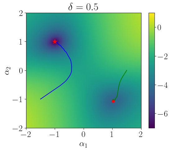
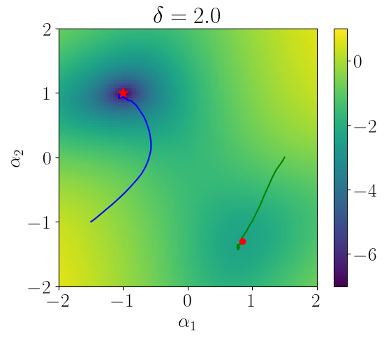
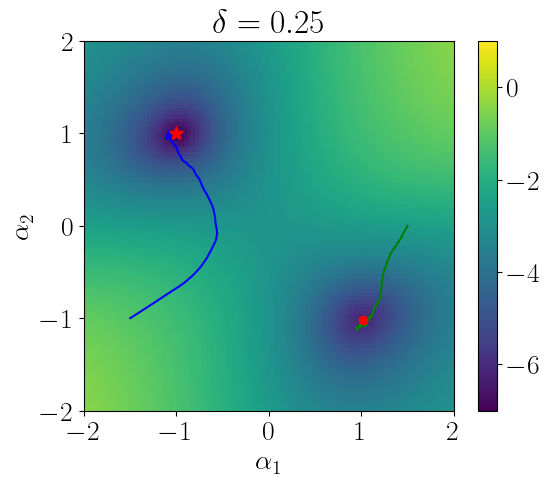
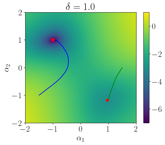
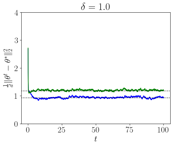
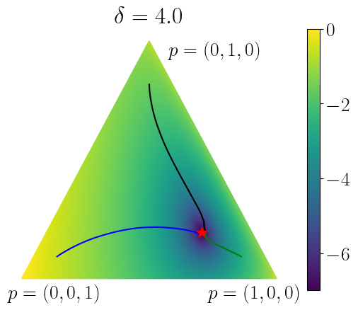
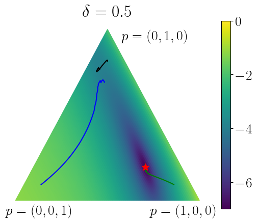
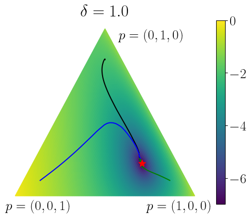
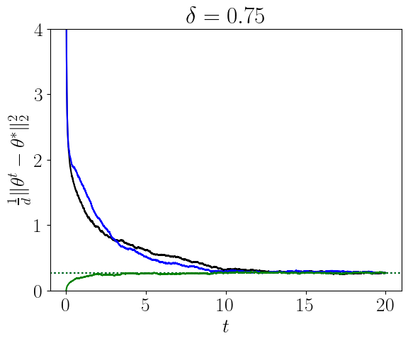
Figure 1: Simulations for the Gaussian mixture prior model 12​𝒩​(α1,1)+12​𝒩​(α2,0.25)\frac{1}{2}\mathcal{N}(\alpha_{1},1)+\frac{1}{2}\mathcal{N}(\alpha_{2},0.25) of Example 2.17, with true mixture means α∗=(1,−1)\alpha^{*}=(1,-1) and linear model noise variance σ2=δ​s2\sigma^{2}=\delta s^{2} for s=0.5s=0.5. Empirical Bayes Langevin dynamics is run for a single instance (𝐗,𝐲)(\mathbf{X},\mathbf{y}) with max⁡(n,d)=5000\max(n,d)=5000, initialization θj0​∼i​i​d​𝒩​(0,1)\theta_{j}^{0}\overset{iid}{\sim}\mathcal{N}(0,1), and an Euler-Maruyama discretization of the dynamics. (a–e) Landscape of the replica-symmetric free energy F⁡(α)F(\alpha) plotted (for visual clarity) as log⁡(F⁡(α)−F⁡(α∗)+10−3)\log(F(\alpha)-F(\alpha^{*})+10^{-3}), for δ∈{4,2,1,0.5,0.25}\delta\in\{4,2,1,0.5,0.25\}. Two stable fixed points of 0=∇F​(α)0=\nabla F(\alpha) are depicted in red, with star indicating the true parameter α∗=(−1,1)\alpha^{*}=(-1,1) and circle indicating a second fixed point α†\alpha^{\dagger} near (1,−1)(1,-1). Sample paths {α^t}t≥0\{\widehat{\alpha}^{t}\}_{t\geq 0} from two different initial states α^0\widehat{\alpha}^{0} are shown in blue and green. (f) Mean-squared-error 1d​‖𝜽t−𝜽∗‖22\frac{1}{d}\|\bm{\theta}^{t}-\bm{\theta}^{*}\|_{2}^{2} across iterations for these same two initial states, at δ=1\delta=1. The predicted value for a posterior sample 𝜽∼𝖯g⁡(⋅,α)(⋅∣𝐗,𝐲)\bm{\theta}\sim\mathsf{P}_{g(\cdot,\alpha)}(\cdot\mid\mathbf{X},\mathbf{y}) is 1d​‖𝜽−𝜽∗‖22≈mse⁡(α)+mse∗⁡(α)\frac{1}{d}\|\bm{\theta}-\bm{\theta}^{*}\|_{2}^{2}\approx\mse(\alpha)+\mse_{*}(\alpha), depicted by dashed lines for α∈{α†,α∗}\alpha\in\{\alpha^{\dagger},\alpha^{*}\}.
Example 2.17.

Consider a KK-component Gaussian mixture prior

g⁡(θ,α)=∑k=1Kpk​ωk2​π​exp⁡(−ωk2​(θ−αk)2)g(\theta,\alpha)=\sum_{k=1}^{K}p_{k}\sqrt{\frac{\omega_{k}}{2\pi}}\exp\Big({-}\frac{\omega_{k}}{2}(\theta-\alpha_{k})^{2}\Big)

with fixed mixture weights p1,…,pKp_{1},\ldots,p_{K} and variances ω1−1,…,ωK−1\omega_{1}^{-1},\ldots,\omega_{K}^{-1}, parametrized by the mixture means α∈ℝK\alpha\in\mathbb{R}^{K}. Let us suppose that g∗​(θ)=g⁡(θ,α∗)g_{*}(\theta)=g(\theta,\alpha^{*}) for some α∗∈ℝK\alpha^{*}\in\mathbb{R}^{K}, and the variances ω1−1,…,ωK−1\omega_{1}^{-1},\ldots,\omega_{K}^{-1} are distinct. We consider the empirical Bayes dynamics driven by

𝒢⁡(α,𝖯)=𝔼θ∼𝖯​[∇α​log​g​(θ,α)]−∇R​(α),\mathcal{G}(\alpha,\mathsf{P})=\mathbb{E}_{\theta\sim\mathsf{P}}[\nabla_{\alpha}\log g(\theta,\alpha)]-\nabla R(\alpha),

where R⁡(α)R(\alpha) is a regularizer of the form (54–55) for which α0,α∗∈ℬ⁡(D)\alpha^{0},\alpha^{*}\in\mathcal{B}(D).

We verify in Section 5.2 that Assumption 2.2(b) holds. Then, for fixed s2>0s^{2}>0 and all sufficiently large δ\delta, Proposition 2.16 ensures that the confinement and log-Sobolev conditions of Assumption 2.11 also hold, and the proposition further establishes a 1-to-1 correspondence between the critical points of FF and the (non-singular) critical points of Gs2​(α)G_{s^{2}}(\alpha) in ℬ⁡(D)\mathcal{B}(D). We note that, here, Gs2​(α)G_{s^{2}}(\alpha) is the negative population log-likelihood in the Gaussian mixture model

𝖯g⁡(⋅,α),s−2​(y)=∑k=1Kpk⋅12​π​(ωk−1+s2)​exp⁡(−12​(ωk−1+s2)​(y−αk)2)\mathsf{P}_{g(\cdot,\alpha),s^{-2}}(y)=\sum_{k=1}^{K}p_{k}\cdot\frac{1}{\sqrt{2\pi(\omega_{k}^{-1}+s^{2})}}\exp\Big({-}\frac{1}{2(\omega_{k}^{-1}+s^{2})}(y-\alpha_{k})^{2}\Big) (57)

having the same mixture means α∈ℝK\alpha\in\mathbb{R}^{K} as the prior, and elevated mixture variances ωk−1+s2\omega_{k}^{-1}+s^{2}. The optimization landscape of Gs2​(α)G_{s^{2}}(\alpha) is well-studied in the literature, see e.g. [73, 74, 75, 76], and in general Gs2​(α)G_{s^{2}}(\alpha) may have local minimizers in ℬ⁡(D)\mathcal{B}(D) that are different from α∗\alpha^{*}. In such settings, Proposition 2.16 implies that Crit\Crit must also have critical points different from α∗\alpha^{*} for large δ\delta.

We depict in Figure 1 a simulation of the landscape of F⁡(α)F(\alpha) and the dynamics (9–10) across a range of values δ∈[0.25,4]\delta\in[0.25,4], in a simple setting of 12​𝒩​(α1,1)+12​𝒩​(α2,0.25)\frac{1}{2}\mathcal{N}(\alpha_{1},1)+\frac{1}{2}\mathcal{N}(\alpha_{2},0.25) with K=2K=2 mixture components and true mixture means α∗=(−1,1)\alpha^{*}=(-1,1). The Almeida-Thouless condition for stability of the replica-symmetric phase was computed in [31, Eq. (25)] to be (in our notation)

1−ω2δ​𝔼g∗,ω∗​[Varg,ω⁡[θ]2]≥01-\frac{\omega^{2}}{\delta}\mathbb{E}_{g_{*},\omega_{*}}[\Var_{g,\omega}[\theta]^{2}]\geq 0 (58)

where g⁡(⋅)=g⁡(⋅,α)g(\cdot)=g(\cdot,\alpha) and (ω,ω∗)=(ω⁡(α),ω∗​(α))(\omega,\omega_{*})=(\omega(\alpha),\omega_{*}(\alpha)). We have verified that this condition holds at each tested δ>0\delta>0 and parameter α∈ℝK\alpha\in\mathbb{R}^{K} depicted in Figure 1, and thus we conjecture that the depicted replica-symmetric free energy function F⁡(α)F(\alpha) is indeed the correct asymptotic limit of −1d​log⁡𝖯g⁡(⋅,α)​(𝐲∣𝐗)-\frac{1}{d}\log\mathsf{P}_{g(\cdot,\alpha)}(\mathbf{y}\mid\mathbf{X}) as n,d→∞n,d\to\infty (even in settings where our assumption of a log-Sobolev inequality for the posterior law may not hold). We observe, not only for large δ\delta but across a range of values δ∈[0.25,4]\delta\in[0.25,4], that the landscape F⁡(α)F(\alpha) has two local minimizers, one fixed at the true parameter α∗=(−1,1)\alpha^{*}=(-1,1) and a second minimizer α†\alpha^{\dagger} whose location depends on δ\delta. As δ\delta decreases, this second minimizer approaches (1,−1)(1,-1) — characterizing a prior law with mixture means matching those of g∗=g⁡(⋅,α∗)g_{*}=g(\,\cdot\,,\alpha^{*}) but with the mixture variances reversed — and the free energy difference F⁡(α†)−F⁡(α∗)F(\alpha^{\dagger})-F(\alpha^{*}) approaches 0, indicating that it becomes increasingly difficult to distinguish α†\alpha^{\dagger} from the true parameter α∗\alpha^{*}. The dynamics {α^t}t≥0\{\widehat{\alpha}^{t}\}_{t\geq 0} follow a smooth trajectory to one of α†\alpha^{\dagger} or α∗\alpha^{*}, depending on the initial state α^0\widehat{\alpha}^{0}.

Refer to caption

(a)

Refer to caption

(d)

Refer to caption

(b)

Refer to caption

(e)

Refer to caption

(c)

Refer to caption

(f)

Figure 2: Simulations for the Gaussian mixture prior model p1​(α)​𝒩​(0,0.04)+p2​(α)​𝒩​(0,1)+p3​(α)​𝒩​(0,25)p_{1}(\alpha)\mathcal{N}(0,0.04)+p_{2}(\alpha)\mathcal{N}(0,1)+p_{3}(\alpha)\mathcal{N}(0,25) of Example 2.18, with true weights p⁡(α∗)=(0.6,0.2,0.2)p(\alpha^{*})=(0.6,0.2,0.2) and linear model noise variance σ2=δ​s2\sigma^{2}=\delta s^{2} for s=0.2s=0.2. Empirical Bayes Langevin dynamics are run for two initializations α^0\widehat{\alpha}^{0} with random θj0​∼i​i​d​𝒩​(0,1)\theta_{j}^{0}\overset{iid}{\sim}\mathcal{N}(0,1) (black and blue), and an initialization α^0\widehat{\alpha}^{0} near α∗\alpha^{*} with ground truth θj0=θj∗\theta_{j}^{0}=\theta_{j}^{*} (green). The remaining setup is the same as in Figure 1. (a–e) Landscape of the replica-symmetric free energy F⁡(α)F(\alpha) for δ∈{4,2,1,0.75,0.5}\delta\in\{4,2,1,0.75,0.5\}, plotted as log⁡(F⁡(α)−F⁡(α∗)+10−3)\log(F(\alpha)-F(\alpha^{*})+10^{-3}) in the coordinates p⁡(α)p(\alpha) on the simplex. The unique critical point p⁡(α∗)p(\alpha^{*}) is depicted as the red star. Sample paths of {p⁡(α^t)}t≥0\{p(\widehat{\alpha}^{t})\}_{t\geq 0} are shown in green, black, and blue. (f) Mean-squared-error 1d​‖𝜽t−𝜽∗‖22\frac{1}{d}\|\bm{\theta}^{t}-\bm{\theta}^{*}\|_{2}^{2} across iterations for these same three initial states, at δ=0.75\delta=0.75. The predicted value of mse⁡(α∗)+mse∗⁡(α∗)\mse(\alpha^{*})+\mse_{*}(\alpha^{*}) for a posterior sample is depicted by the dashed line.
Example 2.18.

Consider a K+1K+1-component Gaussian mixture prior

g⁡(θ,α)=∑k=0Kpk​(α)​ωk2​π​exp⁡(−ωk2​(θ−μk)2),pk​(α)=eαkeα0+…+eαKg(\theta,\alpha)=\sum_{k=0}^{K}p_{k}(\alpha)\sqrt{\frac{\omega_{k}}{2\pi}}\exp\Big({-}\frac{\omega_{k}}{2}(\theta-\mu_{k})^{2}\Big),\qquad p_{k}(\alpha)=\frac{e^{\alpha_{k}}}{e^{\alpha_{0}}+\ldots+e^{\alpha_{K}}}

with fixed means μ0,…,μK\mu_{0},\ldots,\mu_{K} and variances ω0−1,…,ωK−1\omega_{0}^{-1},\ldots,\omega_{K}^{-1}, parametrized instead by the mixture weights pk​(α)=eαk/(eα0+…+eαK)p_{k}(\alpha)=e^{\alpha_{k}}/(e^{\alpha_{0}}+\ldots+e^{\alpha_{K}}). Let us suppose that g∗​(θ)=g⁡(θ,α∗)g_{*}(\theta)=g(\theta,\alpha^{*}) for some α∗∈ℝK+1\alpha^{*}\in\mathbb{R}^{K+1}, and the parameter pairs (μ0,ω0),…,(μK,ωK)(\mu_{0},\omega_{0}),\ldots,(\mu_{K},\omega_{K}) are distinct. We again consider the dynamics driven by

𝒢⁡(α,𝖯)=𝔼θ∼𝖯​[∇α​log​g​(θ,α)]−∇R​(α),\mathcal{G}(\alpha,\mathsf{P})=\mathbb{E}_{\theta\sim\mathsf{P}}[\nabla_{\alpha}\log g(\theta,\alpha)]-\nabla R(\alpha),

where R⁡(α)R(\alpha) is a regularizer of the form (54–55) such that α0,α∗∈ℬ⁡(D)\alpha^{0},\alpha^{*}\in\mathcal{B}(D). This parametrization is overparametrized by a single parameter — however, defining the KK-dimensional linear subspace E={α∈ℝK+1:α0+…+αK=0}E=\{\alpha\in\mathbb{R}^{K+1}:\alpha_{0}+\ldots+\alpha_{K}=0\}, a direct calculation (c.f. Section 5.2) verifies that ∇α​log​g​(θ,α)∈E\nabla_{\alpha}\log g(\theta,\alpha)\in E and ∇R​(α)∈E\nabla R(\alpha)\in E if α∈E\alpha\in E. Thus, initializing α^0∈E\widehat{\alpha}^{0}\in E ensures α^t∈E\widehat{\alpha}^{t}\in E for all t≥0t\geq 0, and we may apply our preceding results upon identifying EE isometrically with ℝK\mathbb{R}^{K}.

We verify in Section 5.2 that Assumption 2.2(b) holds. Then again for fixed s2>0s^{2}>0 and all large δ\delta, Proposition 2.16 ensures that Assumption 2.11 also holds, and there is a 1-to-1 correspondence between the critical points of FF and Gs2​(α)G_{s^{2}}(\alpha) on ℬ⁡(D)\mathcal{B}(D). Here, Gs2​(α)G_{s^{2}}(\alpha) is the negative population log-likelihood of the Gaussian mixture model

𝖯g⁡(⋅,α),s−2​(y)=∑k=0Kpk​(α)​12​π​(ωk−1+s2)​exp⁡(−12​(ωk−1+s2)​(y−μk)2).\mathsf{P}_{g(\cdot,\alpha),s^{-2}}(y)=\sum_{k=0}^{K}p_{k}(\alpha)\sqrt{\frac{1}{2\pi(\omega_{k}^{-1}+s^{2})}}\exp\Big({-}\frac{1}{2(\omega_{k}^{-1}+s^{2})}(y-\mu_{k})^{2}\Big). (59)

Letting S={(p0,…,pK):p0+…+pK=1,p0,…,pK>0}S=\{(p_{0},\ldots,p_{K}):p_{0}+\ldots+p_{K}=1,\,p_{0},\ldots,p_{K}>0\} be the open probability simplex, the mapping α∈E↦p⁡(α)∈S\alpha\in E\mapsto p(\alpha)\in S is a 1-to-1 smooth parametrization with smooth inverse, and the function Gs2G_{s^{2}} is strictly convex in the parametrization by (p0,…,pK)∈S(p_{0},\ldots,p_{K})\in S. Thus p∗=p⁡(α∗)∈Sp^{*}=p(\alpha^{*})\in S is the unique critical point where ∇pGs2=0\nabla_{p}G_{s^{2}}=0, and the Hessian ∇p2Gs2\nabla_{p}^{2}G_{s^{2}} is nonsingular at p∗p^{*}. This implies that α∗∈E\alpha^{*}\in E is also the unique critical point where ∇αGs2=0\nabla_{\alpha}G_{s^{2}}=0, and ∇α2Gs2\nabla_{\alpha}^{2}G_{s^{2}} is also non-singular at α∗\alpha^{*}. So for large δ\delta, Proposition 2.16 ensures that α∗\alpha^{*} must be the unique point of Crit∩ℬ⁡(D)\Crit\cap\,\mathcal{B}(D).

Figure 2 depicts the simulated landscape of F⁡(α)F(\alpha) and dynamics (9–10) in a scaled-mixture-of-normals model p1​(α)​𝒩​(0,0.04)+p2​(α)​𝒩​(0,1)+p3​(α)​𝒩​(0,25)p_{1}(\alpha)\mathcal{N}(0,0.04)+p_{2}(\alpha)\mathcal{N}(0,1)+p_{3}(\alpha)\mathcal{N}(0,25) with all components having mean 0, across a range of values δ∈[0.5,4]\delta\in[0.5,4], and with true weights p⁡(α∗)=(0.6,0.2,0.2)p(\alpha^{*})=(0.6,0.2,0.2). (We have again verified that the Almeida-Thouless stability condition (58) holds at each depicted δ>0\delta>0 and parameter value α∈ℝK\alpha\in\mathbb{R}^{K} in these figures.) We observe for all tested values δ∈[0.5,4]\delta\in[0.5,4] that α∗\alpha^{*} is the unique local minimizer and critical point of F⁡(α)F(\alpha). However, as δ\delta decreases, the landscape of F⁡(α)F(\alpha) flattens around α∗\alpha^{*} along a direction representing a family of priors g⁡(⋅,α)g(\,\cdot\,,\alpha) having the same first two moments as g⁡(⋅,α∗)g(\,\cdot\,,\alpha^{*}), reflecting that the problem of learning g⁡(⋅,α∗)g(\,\cdot\,,\alpha^{*}) beyond its second moment becomes increasingly ill-conditioned. The learned parameter {α^t}t≥0\{\widehat{\alpha}^{t}\}_{t\geq 0} successfully converges to α∗\alpha^{*} from several different initial states α^0\widehat{\alpha}^{0} when δ≥0.75\delta\geq 0.75, with mixing of Langevin dynamics becoming increasingly slower as δ\delta decreases. For δ=0.5\delta=0.5, the learned parameter {α^t}t≥0\{\widehat{\alpha}^{t}\}_{t\geq 0} fails to converge to α∗\alpha^{*} under the tested time horizon from random initializations of 𝜽0\bm{\theta}^{0}, but does converge to α∗\alpha^{*} under a ground-truth initialization 𝜽0=𝜽∗\bm{\theta}^{0}=\bm{\theta}^{*} and α^0\widehat{\alpha}^{0} close to α∗\alpha^{*}.

3 Analysis of approximately-TTI DMFT systems

In this section, we prove Theorem 2.5 on the equilibrium properties of the solution to the DMFT equations under an assumption of approximate time-translation-invariance (from an out-of-equilibrium initialization). We assume throughout this section that Assumptions 2.1 and 2.2(a) hold, and that the solution to the DMFT system in Theorem 2.3(a) approximating the dynamics (7) with the fixed prior g⁡(⋅)g(\cdot) is approximately-TTI in the sense of Definition 2.4. We denote by {θt}t≥0\{\theta^{t}\}_{t\geq 0}, {ηt}t≥0\{\eta^{t}\}_{t\geq 0}, and Cθ,Cη,Rθ,RηC_{\theta},C_{\eta},R_{\theta},R_{\eta} the components of this DMFT solution.

3.1 Analysis of θ\theta-equation

We first derive, from analysis of the evolution (23) for {θt}t≥0\{\theta^{t}\}_{t\geq 0}, a representation of cθtti​(0),cθtti​(∞),cθ​(∗)c_{\theta}^{\mathrm{tti}}(0),c_{\theta}^{\mathrm{tti}}(\infty),c_{\theta}(*) in terms of cηtti​(0),cηtti​(∞)c_{\eta}^{\mathrm{tti}}(0),c_{\eta}^{\mathrm{tti}}(\infty), assuming a condition cηtti​(0)−cηtti​(∞)<δ/σ2c_{\eta}^{\mathrm{tti}}(0)-c_{\eta}^{\mathrm{tti}}(\infty)<\delta/\sigma^{2} which ensures long-time stability of {θt}t≥0\{\theta^{t}\}_{t\geq 0} under (23). This condition will be checked in our subsequent analysis of the evolution of {ηt}t≥0\{\eta^{t}\}_{t\geq 0}.

Lemma 3.1.

Suppose cηtti​(0)−cηtti​(∞)<δ/σ2c_{\eta}^{\mathrm{tti}}(0)-c_{\eta}^{\mathrm{tti}}(\infty)<\delta/\sigma^{2}. Set ω=δ/σ2−(cηtti​(0)−cηtti​(∞))\omega=\delta/\sigma^{2}-(c_{\eta}^{\mathrm{tti}}(0)-c_{\eta}^{\mathrm{tti}}(\infty)) and ω∗=ω2/cηtti​(∞)\omega_{\ast}=\omega^{2}/c_{\eta}^{\mathrm{tti}}(\infty). Then

cθtti​(0)=𝔼g∗,ω∗​⟨θ2⟩g,ω,cθtti​(∞)=𝔼g∗,ω∗​⟨θ⟩g,ω2,cθ​(∗)=𝔼g∗,ω∗​[⟨θ⟩g,ω​θ∗].\displaystyle c_{\theta}^{\mathrm{tti}}(0)=\mathbb{E}_{g_{\ast},\omega_{*}}\langle\theta^{2}\rangle_{g,\omega},\quad c_{\theta}^{\mathrm{tti}}(\infty)=\mathbb{E}_{g_{\ast},\omega_{*}}\langle\theta\rangle_{g,\omega}^{2},\quad c_{\theta}(\ast)=\mathbb{E}_{g_{\ast},\omega_{*}}[\langle\theta\rangle_{g,\omega}\theta^{\ast}]. (60)

The main idea of the proof is to apply the explicit form of cθttic_{\theta}^{\mathrm{tti}} in (33) together with its fluctuation dissipation relation with rθttir_{\theta}^{\mathrm{tti}} in (36) to approximate Cθ,RθC_{\theta},R_{\theta} at large times by correlation and response functions Cθ(M),Rθ(M)C_{\theta}^{(M)},R_{\theta}^{(M)} that admit an interpretation as the effect of marginalization over auxiliary variables (x1t,…,xMt)(x_{1}^{t},\ldots,x_{M}^{t}) in a Markovian joint evolution of (θt,x1t,…,xMt)(\theta^{t},x_{1}^{t},\ldots,x_{M}^{t}) conditional on θ∗\theta^{*}. In contrast to the original high-dimensional dynamics of {𝜽t}t≥0\{\bm{\theta}^{t}\}_{t\geq 0} in ℝd\mathbb{R}^{d}, here MM does not depend on (n,d)(n,d), and the dynamics of {x1t,…,xMt}\{x_{1}^{t},\ldots,x_{M}^{t}\} will be decoupled given {θt}t≥0\{\theta^{t}\}_{t\geq 0}. This decoupling allows us to provide a simple explicit form for the θ\theta-marginal of the stationary distribution of (θ,x1,…,xM)(\theta,x_{1},\ldots,x_{M}) conditional on θ∗\theta^{*}, which in the limit M→∞M\to\infty will match the conditional distribution θ|θ∗\theta\mid\theta^{*} under the limit law 𝖯g∗,ω∗;g,ω​(θ,θ∗)\mathsf{P}_{g_{*},\omega_{*};g,\omega}(\theta,\theta^{*}).

To implement this idea, we will exhibit a coupling of the processes {θt}t≥0\{\theta^{t}\}_{t\geq 0} driven by Cθ,RθC_{\theta},R_{\theta} and {θM,T0t}t≥0\{\theta_{M,T_{0}}^{t}\}_{t\geq 0} driven by Cθ(M),Rθ(M)C_{\theta}^{(M)},R_{\theta}^{(M)} from time T0T_{0} onwards, and then analyze the convergence of {θM,T0t}t≥0\{\theta_{M,T_{0}}^{t}\}_{t\geq 0} under the equivalent Markovian representation of its dynamics. The main technical challenge is to ensure either that the discretization error ε⁡(M)\varepsilon(M) obtained by approximating Cθ,RθC_{\theta},R_{\theta} by Cθ(M),Rθ(M)C_{\theta}^{(M)},R_{\theta}^{(M)} does not compound exponentially over time, or that the convergence time of {θM,T0t}t≥0\{\theta^{t}_{M,T_{0}}\}_{t\geq 0} in the equivalent Markovian dynamics is independent of the approximation dimension MM. We will take the first approach here, by adapting ideas around sticky and reflection couplings developed in [77, 78] to a setting of non-Markovian DMFT dynamics for {θt}t≥0\{\theta^{t}\}_{t\geq 0} and {θM,T0t}t≥0\{\theta_{M,T_{0}}^{t}\}_{t\geq 0}.

3.1.1 Comparison with an auxiliary process

Let us fix a positive integer MM and define two sequences {am}m=0M\{a_{m}\}_{m=0}^{M} and {cm}m=1M\{c_{m}\}_{m=1}^{M} by

am=ι+mM​ for ​m=0,…,M,cm2am=μη​([am−1,am))​ for ​m=1,…,M\displaystyle a_{m}=\iota+\frac{m}{\sqrt{M}}\text{ for }m=0,\ldots,M,\qquad\frac{c_{m}^{2}}{a_{m}}=\mu_{\eta}([a_{m-1},a_{m}))\text{ for }m=1,\ldots,M (61)

where μη\mu_{\eta} is given in Definition 2.4. We set

Rη(M)​(τ)=∑m=1Mcm2​e−am​τ,Cη(M)​(t,s)=∑m=1Mcm2am​(e−am​|t−s|−e−am​(t+s))+cηtti​(∞).R_{\eta}^{(M)}(\tau)=\sum_{m=1}^{M}c_{m}^{2}e^{-a_{m}\tau},\qquad C_{\eta}^{(M)}(t,s)=\sum_{m=1}^{M}\frac{c_{m}^{2}}{a_{m}}(e^{-a_{m}|t-s|}-e^{-a_{m}(t+s)})+c_{\eta}^{\mathrm{tti}}(\infty).

A direct calculation of the covariance shows that

Cη(M)​(t,s)=𝔼⁡[uMt​uMs] for uMt=z+∑m=1Mcm​∫0te−am​(t−s)​2​d​bms,C_{\eta}^{(M)}(t,s)=\mathbb{E}[u_{M}^{t}u_{M}^{s}]\quad\text{ for }\quad u_{M}^{t}=z+\sum_{m=1}^{M}c_{m}\int_{0}^{t}e^{-a_{m}(t-s)}\sqrt{2}\,\mathrm{d}b_{m}^{s}, (62)

where z∼𝒩⁡(0,cηtti​(∞))z\sim\mathcal{N}(0,c_{\eta}^{\mathrm{tti}}(\infty)) and {b1t}t≥0,…,{bMt}t≥0\{b_{1}^{t}\}_{t\geq 0},\ldots,\{b_{M}^{t}\}_{t\geq 0} are standard Brownian motions independent of each other and of zz. In particular, Cη(M)​(t,s)C_{\eta}^{(M)}(t,s) is a positive-semidefinite covariance kernel on [0,∞)[0,\infty).

For convenience, let us set

U⁡(θ,θ∗)=−δσ2​(θ−θ∗)+(log⁡g)′​(θ),U(\theta,\theta^{\ast})=-\frac{\delta}{\sigma^{2}}(\theta-\theta^{\ast})+(\log g)^{\prime}(\theta),

so the DMFT equation (23) reads

d​θt=[U⁡(θt,θ∗)+∫0tRη​(t,s)​(θs−θ∗)​𝑑s+ut]​𝑑t+2​d​bt.\displaystyle\mathrm{d}\theta^{t}=\Big[U(\theta^{t},\theta^{\ast})+\int_{0}^{t}R_{\eta}(t,s)(\theta^{s}-\theta^{\ast})\mathrm{d}s+u^{t}\Big]\mathrm{d}t+\sqrt{2}\,\mathrm{d}b^{t}. (63)

Let {uMt}t≥0\{u_{M}^{t}\}_{t\geq 0} be a centered Gaussian process with covariance kernel Cη(M)C_{\eta}^{(M)}, defined in the probability space of {ut,θt}t≥0\{u^{t},\theta^{t}\}_{t\geq 0} and independent of θ∗\theta^{*}. Fixing a time T0>0T_{0}>0, let {b~t}t≥T0\{\tilde{b}^{t}\}_{t\geq T_{0}} be a standard Brownian motion initialized at b~T0=0\tilde{b}^{T_{0}}=0, independent of {ut}t≥0\{u^{t}\}_{t\geq 0}, θ∗\theta^{*}, and {θt}t∈[0,T]\{\theta^{t}\}_{t\in[0,T]}. We consider an auxiliary process {θM,T0t}t≥0\{\theta_{M,T_{0}}^{t}\}_{t\geq 0} defined by

θM,T0t\displaystyle\theta_{M,T_{0}}^{t} =θt​ for ​t∈[0,T0],\displaystyle=\theta^{t}\text{ for }t\in[0,T_{0}], (64)
d​θM,T0t\displaystyle\mathrm{d}\theta_{M,T_{0}}^{t} =[U⁡(θM,T0t,θ∗)+∫0tRη(M)​(t−s)​(θM,T0s−θ∗)​ds+uMt]​dt+2​d​b~t​ for ​t≥T0.\displaystyle=\Big[U(\theta_{M,T_{0}}^{t},\theta^{\ast})+\int_{0}^{t}R_{\eta}^{(M)}(t-s)(\theta_{M,T_{0}}^{s}-\theta^{\ast})\mathrm{d}s+u_{M}^{t}\Big]\mathrm{d}t+\sqrt{2}\,\mathrm{d}\tilde{b}^{t}\text{ for }t\geq T_{0}.

We proceed to construct a coupling of {uMt}t≥0\{u_{M}^{t}\}_{t\geq 0} with {ut}t≥0\{u^{t}\}_{t\geq 0} and of {b~t}t≥T0\{\tilde{b}^{t}\}_{t\geq T_{0}} with {bt−bT0}t≥T0\{b^{t}-b^{T_{0}}\}_{t\geq T_{0}} defining the DMFT solution {θt}t≥0\{\theta^{t}\}_{t\geq 0}, to yield a coupling of {θM,T0t}t≥T0\{\theta_{M,T_{0}}^{t}\}_{t\geq T_{0}} with {θt}t≥T0\{\theta^{t}\}_{t\geq T_{0}}.

Lemma 3.2.

For any M,T0,T>0M,T_{0},T>0, there exists a coupling of {uMt}t≥0\{u_{M}^{t}\}_{t\geq 0} and {ut}t≥0\{u^{t}\}_{t\geq 0} such that

supt∈[T0,T0+T]𝔼​(uMt−ut)2≤ε⁡(M)+T​ε​(T0),\displaystyle\sup_{t\in[T_{0},T_{0}+T]}\mathbb{E}(u_{M}^{t}-u^{t})^{2}\leq\varepsilon(M)+\sqrt{T}\,\varepsilon(T_{0}),

where ε⁡(M)\varepsilon(M) does not depend on T0,TT_{0},T and ε⁡(T0)\varepsilon(T_{0}) does not depend on M,TM,T, and limM→∞ε⁡(M)=0\lim_{M\to\infty}\varepsilon(M)=0 and limT0→∞ε⁡(T0)=0\lim_{T_{0}\to\infty}\varepsilon(T_{0})=0.

Proof.

Define the covariance kernel Cη(∞)​(t,s)=∫ι∞(e−a​|t−s|−e−a⁡(t+s))​μη​(𝑑a)+cηtti​(∞)C_{\eta}^{(\infty)}(t,s)=\int_{\iota}^{\infty}\big(e^{-a|t-s|}-e^{-a(t+s)}\big)\mu_{\eta}(\mathrm{d}a)+c_{\eta}^{\mathrm{tti}}(\infty) representing the M→∞M\to\infty limit of (62). We will couple Gaussian processes with covariance kernels (Cη(M),Cη(∞))(C_{\eta}^{(M)},C_{\eta}^{(\infty)}) and with (Cη(∞),Cη)(C_{\eta}^{(\infty)},C_{\eta}) respectively.

Coupling of (Cη(M),Cη(∞))(C_{\eta}^{(M)},C_{\eta}^{(\infty)}). Let M′>MM^{\prime}>M be any positive integer for which M′\sqrt{M^{\prime}} is an integer multiple of M\sqrt{M}, and let {a~m}m=0M′\{\tilde{a}_{m}\}_{m=0}^{M^{\prime}} and {c~m}m=1M′\{\tilde{c}_{m}\}_{m=1}^{M^{\prime}} be the sequences as defined above with M′M^{\prime} in place of MM. Note then that the grid points {aj}j=0M\{a_{j}\}_{j=0}^{M} are a subset of the grid points {a~i}i=0M′\{\tilde{a}_{i}\}_{i=0}^{M^{\prime}}. Let

uM′t=z+∑i=1M′c~i​∫0te−a~i​(t−s)​2​d​b~is\displaystyle u_{M^{\prime}}^{t}=z+\sum_{i=1}^{M^{\prime}}\tilde{c}_{i}\int_{0}^{t}e^{-\tilde{a}_{i}(t-s)}\sqrt{2}\,\mathrm{d}\tilde{b}^{s}_{i} (65)

where z∼𝒩⁡(0,cηtti​(∞))z\sim\mathcal{N}(0,c_{\eta}^{\mathrm{tti}}(\infty)) and {b~1t}t≥0,…​{b~M′t}t≥0\{\tilde{b}^{t}_{1}\}_{t\geq 0},\ldots\{\tilde{b}^{t}_{M^{\prime}}\}_{t\geq 0} are standard Brownian motions independent of each other and of zz. Then (62) shows that {uM′t}t≥0\{u_{M^{\prime}}^{t}\}_{t\geq 0} has covariance Cη(M′)C_{\eta}^{(M^{\prime})}. Now, for each j=1,…,Mj=1,\ldots,M, let

Ij={i:aj−1<a~i≤aj},bjt=∑i∈Ijc~i​b~it/∑i∈Ijc~i2I_{j}=\{i:a_{j-1}<\tilde{a}_{i}\leq a_{j}\},\qquad b^{t}_{j}=\sum_{i\in I_{j}}\tilde{c}_{i}\tilde{b}^{t}_{i}\bigg/\sqrt{\sum_{i\in I_{j}}\tilde{c}_{i}^{2}}

and set

uMt=z+∑j=1Mcj​∫0te−aj​(t−s)​2​d​bjs.\displaystyle u_{M}^{t}=z+\sum_{j=1}^{M}c_{j}\int_{0}^{t}e^{-a_{j}(t-s)}\sqrt{2}\,\mathrm{d}b^{s}_{j}.

Then {b1t}t≥0,…,{bMt}t≥0\{b^{t}_{1}\}_{t\geq 0},\ldots,\{b^{t}_{M}\}_{t\geq 0} are standard Brownian motions independent of each other and of zz, so (62) shows also that {ut}t≥0\{u^{t}\}_{t\geq 0} is a Gaussian process with covariance Cη(M)C_{\eta}^{(M)}.

We may now bound

𝔼⁡[(uMt−uM′t)2]\displaystyle\mathbb{E}[(u_{M}^{t}-u_{M^{\prime}}^{t})^{2}] ≤4𝔼[(∑i:a~i>aMc~i∫0te−a~i​(t−s)db~is)2]\displaystyle\leq 4\,\mathbb{E}\Big[\Big(\sum_{i:\tilde{a}_{i}>a_{M}}\tilde{c}_{i}\int_{0}^{t}e^{-\tilde{a}_{i}(t-s)}\mathrm{d}\tilde{b}^{s}_{i}\Big)^{2}\Big]
+4​𝔼​[(∑j=1M∑i∈Ijc~i​∫0te−a~i​(t−s)​d​b~si−∑j=1Mcj​∫0te−aj​(t−s)​d​bjs)2].\displaystyle\hskip 72.26999pt+4\,\mathbb{E}\Big[\Big(\sum_{j=1}^{M}\sum_{i\in I_{j}}\tilde{c}_{i}\int_{0}^{t}e^{-\tilde{a}_{i}(t-s)}\mathrm{d}\tilde{b}^{i}_{s}-\sum_{j=1}^{M}c_{j}\int_{0}^{t}e^{-a_{j}(t-s)}\mathrm{d}b^{s}_{j}\Big)^{2}\Big].

Since aM=ι+Ma_{M}=\iota+\sqrt{M}, the first term equals ∑i:a~i>ι+Mc~i2/a~i=∑i:a~i>ι+Mμη([a~i−1,a~i))\sum_{i:\tilde{a}_{i}>\iota+\sqrt{M}}\tilde{c}_{i}^{2}/\tilde{a}_{i}=\sum_{i:\tilde{a}_{i}>\iota+\sqrt{M}}\mu_{\eta}([\tilde{a}_{i-1},\tilde{a}_{i})), which is at most some ε1​(M)\varepsilon_{1}(M) satisfying limM→∞ε1​(M)=0\lim_{M\to\infty}\varepsilon_{1}(M)=0, by finiteness of the measure μη\mu_{\eta}. The second term is bounded as

𝔼⁡[(∑j=1M∑i∈Ijc~i​∫0te−a~i​(t−s)​d​b~is−∑j=1Mcj​∫0te−aj​(t−s)​d​bjs)2]\displaystyle\mathbb{E}\Big[\Big(\sum_{j=1}^{M}\sum_{i\in I_{j}}\tilde{c}_{i}\int_{0}^{t}e^{-\tilde{a}_{i}(t-s)}\mathrm{d}\tilde{b}^{s}_{i}-\sum_{j=1}^{M}c_{j}\int_{0}^{t}e^{-a_{j}(t-s)}\mathrm{d}b^{s}_{j}\Big)^{2}\Big]
=𝔼⁡[(∑j=1M∑i∈Ij∫0t(c~i​e−a~i​(t−s)−cj​c~i∑ℓ∈Ijc~ℓ2​e−aj​(t−s))​d​b~is)2]\displaystyle=\mathbb{E}\Big[\Big(\sum_{j=1}^{M}\sum_{i\in I_{j}}\int_{0}^{t}\Big(\tilde{c}_{i}e^{-\tilde{a}_{i}(t-s)}-\frac{c_{j}\tilde{c}_{i}}{\sqrt{\sum_{\ell\in I_{j}}\tilde{c}_{\ell}^{2}}}e^{-a_{j}(t-s)}\Big)\mathrm{d}\tilde{b}^{s}_{i}\Big)^{2}\Big]
=∑j=1M∑i∈Ij∫0t(c~i​e−a~i​s−cj​c~i∑ℓ∈Ijc~ℓ2​e−aj​s)2​𝑑s≤2​(I+II),\displaystyle=\sum_{j=1}^{M}\sum_{i\in I_{j}}\int_{0}^{t}\Big(\tilde{c}_{i}e^{-\tilde{a}_{i}s}-\frac{c_{j}\tilde{c}_{i}}{\sqrt{\sum_{\ell\in I_{j}}\tilde{c}_{\ell}^{2}}}e^{-a_{j}s}\Big)^{2}\mathrm{d}s\leq 2(\mathrm{I}+\mathrm{II}),

where

I=∑j=1M∑i∈Ij∫0tc~i2​(e−a~i​s−e−aj​s)2​𝑑s,II=∑j=1M∑i∈Ij∫0tc~i2​(1−cj∑ℓ∈Ijc~ℓ2)2​e−2​aj​s​𝑑s.\displaystyle\mathrm{I}=\sum_{j=1}^{M}\sum_{i\in I_{j}}\int_{0}^{t}\tilde{c}_{i}^{2}\big(e^{-\tilde{a}_{i}s}-e^{-a_{j}s}\big)^{2}\mathrm{d}s,\qquad\mathrm{II}=\sum_{j=1}^{M}\sum_{i\in I_{j}}\int_{0}^{t}\tilde{c}_{i}^{2}\Big(1-\frac{c_{j}}{\sqrt{\sum_{\ell\in I_{j}}\tilde{c}_{\ell}^{2}}}\Big)^{2}e^{-2a_{j}s}\mathrm{d}s.

Let Δ=1/M\Delta=1/\sqrt{M} be the spacing of {aj}j=0M\{a_{j}\}_{j=0}^{M}. Then, since |a~i−aj|≤Δ|\tilde{a}_{i}-a_{j}|\leq\Delta and a~i≤aj\tilde{a}_{i}\leq a_{j} for all i∈Iji\in I_{j},

I\displaystyle\mathrm{I} ≤∑j=1M∑i∈Ij∫0tc~i2​e−2​aj−1​s​s2​Δ2​𝑑s≤∑j=1M∫0t(∑i∈Ijc~i2a~i)​aj​e−2​aj−1​s​s2​Δ2​𝑑s=(∗)∑j=1Mcj2​∫0te−2​aj−1​s​s2​Δ2​𝑑s\displaystyle\leq\sum_{j=1}^{M}\sum_{i\in I_{j}}\int_{0}^{t}\tilde{c}_{i}^{2}e^{-2a_{j-1}s}s^{2}\Delta^{2}\mathrm{d}s\leq\sum_{j=1}^{M}\int_{0}^{t}\Big(\sum_{i\in I_{j}}\frac{\tilde{c}_{i}^{2}}{\tilde{a}_{i}}\Big)a_{j}e^{-2a_{j-1}s}s^{2}\Delta^{2}\mathrm{d}s\stackrel{{\scriptstyle(*)}}{{=}}\sum_{j=1}^{M}c_{j}^{2}\int_{0}^{t}e^{-2a_{j-1}s}s^{2}\Delta^{2}\mathrm{d}s

where we use ∑i∈Ijc~i2/a~i=∑i∈Ijμη​([a~i−1,a~i))=μη​([aj−1,aj))=cj2/aj\sum_{i\in I_{j}}\tilde{c}_{i}^{2}/\tilde{a}_{i}=\sum_{i\in I_{j}}\mu_{\eta}([\tilde{a}_{i-1},\tilde{a}_{i}))=\mu_{\eta}([a_{j-1},a_{j}))=c_{j}^{2}/a_{j} in (∗)(\ast). Evaluating this integral, for an absolute constant C>0C>0,

I\displaystyle\mathrm{I} ≤C​Δ2​∑j=1Mcj2aj−13≤C​Δ2ι2​∑j=1Mcj2aj≤C​Δ2ι2​μη​([ι,∞))≤ε2​(M)\displaystyle\leq C\Delta^{2}\sum_{j=1}^{M}\frac{c_{j}^{2}}{a_{j-1}^{3}}\leq\frac{C\Delta^{2}}{\iota^{2}}\sum_{j=1}^{M}\frac{c_{j}^{2}}{a_{j}}\leq\frac{C\Delta^{2}}{\iota^{2}}\mu_{\eta}([\iota,\infty))\leq\varepsilon_{2}(M)

where limM→∞ε2​(M)=0\lim_{M\to\infty}\varepsilon_{2}(M)=0. For II\mathrm{II}, since cj2=∑ℓ∈Ijaja~ℓ​c~ℓ2c_{j}^{2}=\sum_{\ell\in I_{j}}\frac{a_{j}}{\tilde{a}_{\ell}}\tilde{c}_{\ell}^{2}, we have |cj2−∑ℓ∈Ijc~ℓ2|≤Δ​∑ℓ∈Ijc~ℓ2/a~ℓ=Δ​cj2/aj|c_{j}^{2}-\sum_{\ell\in I_{j}}\tilde{c}_{\ell}^{2}|\leq\Delta\sum_{\ell\in I_{j}}\tilde{c}_{\ell}^{2}/\tilde{a}_{\ell}=\Delta c_{j}^{2}/a_{j}, and hence

II≤∑j=1M∑i∈Ijc~i22​aj​(cj−∑ℓ∈Ijc~ℓ2)2∑ℓ∈Ijc~ℓ2≤∑j=1M(cj2−∑ℓ∈Ijc~ℓ2)22​aj​cj2≤Δ22​∑j=1Mcj2aj3≤Δ22​ι2​∑j=1Mcj2aj≤ε3​(M)\displaystyle\mathrm{II}\leq\sum_{j=1}^{M}\sum_{i\in I_{j}}\frac{\tilde{c}_{i}^{2}}{2a_{j}}\frac{(c_{j}-\sqrt{\sum_{\ell\in I_{j}}\tilde{c}_{\ell}^{2}})^{2}}{\sum_{\ell\in I_{j}}\tilde{c}_{\ell}^{2}}\leq\sum_{j=1}^{M}\frac{(c_{j}^{2}-\sum_{\ell\in I_{j}}\tilde{c}_{\ell}^{2})^{2}}{2a_{j}c_{j}^{2}}\leq\frac{\Delta^{2}}{2}\sum_{j=1}^{M}\frac{c_{j}^{2}}{a_{j}^{3}}\leq\frac{\Delta^{2}}{2\iota^{2}}\sum_{j=1}^{M}\frac{c_{j}^{2}}{a_{j}}\leq\varepsilon_{3}(M)

where limM→∞ε3​(M)=0\lim_{M\to\infty}\varepsilon_{3}(M)=0. In summary, we have shown that supt≥0𝔼⁡[(uMt−uM′t)2]≤ε⁡(M)\sup_{t\geq 0}\mathbb{E}[(u_{M}^{t}-u_{M^{\prime}}^{t})^{2}]\leq\varepsilon(M) for some ε⁡(M)→0\varepsilon(M)\rightarrow 0 as M→∞M\rightarrow\infty.

Now note that for any fixed T0T_{0} and TT, {uM′t}t∈[T0,T0+T]\{u_{M^{\prime}}^{t}\}_{t\in[T_{0},T_{0}+T]} has covariance kernel Cη(M′)C_{\eta}^{(M^{\prime})} that converges uniformly to Cη(∞)C_{\eta}^{(\infty)} over [T0,T0+T][T_{0},T_{0}+T] as M′→∞M^{\prime}\rightarrow\infty. It is direct to check from its definitions that Cη(∞)C_{\eta}^{(\infty)} satisfies the condition (235) of Lemma D.1. So by Lemma D.1, there exists a coupling of {uM′t}t∈[T0,T0+T]\{u_{M^{\prime}}^{t}\}_{t\in[T_{0},T_{0}+T]} and a Gaussian process {u∞t}t∈[T0,T0+T]\{u_{\infty}^{t}\}_{t\in[T_{0},T_{0}+T]} with covariance {Cη(∞)​(t,s)}s,t∈[T0,T0+T]\{C_{\eta}^{(\infty)}(t,s)\}_{s,t\in[T_{0},T_{0}+T]} such that supt∈[T0,T0+T]𝔼​(uM′t−u∞t)2→0\sup_{t\in[T_{0},T_{0}+T]}\mathbb{E}(u_{M^{\prime}}^{t}-u_{\infty}^{t})^{2}\rightarrow 0 as M′→∞M^{\prime}\rightarrow\infty. Combining this with the above bound supt≥0𝔼⁡[(uMt−uM′t)2]≤ε⁡(M)\sup_{t\geq 0}\mathbb{E}[(u_{M}^{t}-u_{M^{\prime}}^{t})^{2}]\leq\varepsilon(M) and taking M′→∞M^{\prime}\to\infty shows supt∈[T0,T0+T]𝔼​(uMt−u∞t)2≤ε⁡(M)\sup_{t\in[T_{0},T_{0}+T]}\mathbb{E}(u_{M}^{t}-u_{\infty}^{t})^{2}\leq\varepsilon(M).

Coupling of (Cη(∞),Cη)(C_{\eta}^{(\infty)},C_{\eta}). By the approximation (31) for CηC_{\eta} in Definition 2.4, we have for any t≥s≥0t\geq s\geq 0 that

|Cη​(t,s)−Cη(∞)​(t,s)|≤ε⁡(s)+∫ι∞e−a⁡(t+s)​d​μη​(a),|C_{\eta}(t,s)-C_{\eta}^{(\infty)}(t,s)|\leq\varepsilon(s)+\int_{\iota}^{\infty}e^{-a(t+s)}\mathrm{d}\mu_{\eta}(a),

so there exists a (different) function ε⁡(T0)\varepsilon(T_{0}) with limT0→∞ε⁡(T0)=0\lim_{T_{0}\to\infty}\varepsilon(T_{0})=0 such that

sups,t∈[T0,T0+T]|Cη​(t,s)−Cη(∞)​(t,s)|≤ε⁡(T0).\sup_{s,t\in[T_{0},T_{0}+T]}|C_{\eta}(t,s)-C_{\eta}^{(\infty)}(t,s)|\leq\varepsilon(T_{0}).

Here Cη(∞)C_{\eta}^{(\infty)} satisfies (235) for a constant C0>0C_{0}>0 depending only on μη\mu_{\eta}, so by Lemma D.1, there exists a coupling of {u∞t}t∈[T0,T0+T]\{u_{\infty}^{t}\}_{t\in[T_{0},T_{0}+T]} with {ut}t∈[T0,T0+T]\{u^{t}\}_{t\in[T_{0},T_{0}+T]}, the latter having covariance {Cη​(t,s)}s,t∈[T0,T0+T]\{C_{\eta}(t,s)\}_{s,t\in[T_{0},T_{0}+T]}, for which supt∈[T0,T0+T]𝔼​(u∞t−ut)2≤C⁡(T​ε​(T0)+ε⁡(T0))\sup_{t\in[T_{0},T_{0}+T]}\mathbb{E}(u_{\infty}^{t}-u^{t})^{2}\leq C(\sqrt{T\,\varepsilon(T_{0})}+\varepsilon(T_{0})) for a constant C>0C>0.

Combining these two couplings yields a coupling of {uMt}t∈[T0,T0+T]\{u_{M}^{t}\}_{t\in[T_{0},T_{0}+T]} with {ut}t∈[T0,T0+T]\{u^{t}\}_{t\in[T_{0},T_{0}+T]} such that supt∈[T0,T0+T]𝔼​(uMt−ut)2≤ε⁡(M)+C⁡(T​ε​(T0)+ε⁡(T0))\sup_{t\in[T_{0},T_{0}+T]}\mathbb{E}(u_{M}^{t}-u^{t})^{2}\leq\varepsilon(M)+C(\sqrt{T\,\varepsilon(T_{0})}+\varepsilon(T_{0})), and extending this arbitrarily to a full coupling of {uMt}t≥0\{u_{M}^{t}\}_{t\geq 0} and {ut}t≥0\{u^{t}\}_{t\geq 0} and adjusting the value of ε⁡(T0)\varepsilon(T_{0}) shows the lemma. ∎

Lemma 3.3.

Suppose cηtti​(0)−cηtti​(∞)<δ/σ2c_{\eta}^{\mathrm{tti}}(0)-c_{\eta}^{\mathrm{tti}}(\infty)<\delta/\sigma^{2}. Then for any M,T0,T>0M,T_{0},T>0, there exists a coupling of the processes {θt}t≥0\{\theta^{t}\}_{t\geq 0} and {θM,T0t}t≥0\{\theta_{M,T_{0}}^{t}\}_{t\geq 0} defined by (63) and (64) such that

supt∈[0,T0+T]𝔼​|θt−θM,T0t|≤ε⁡(M)+T​ε​(T0),\displaystyle\sup_{t\in[0,T_{0}+T]}\mathbb{E}|\theta^{t}-\theta_{M,T_{0}}^{t}|\leq\varepsilon(M)+\sqrt{T}\,\varepsilon(T_{0}),

where ε⁡(M)\varepsilon(M) does not depend on T0,TT_{0},T and ε⁡(T0)\varepsilon(T_{0}) does not depend on M,TM,T, and limM→∞ε⁡(M)=0\lim_{M\to\infty}\varepsilon(M)=0 and limT0→∞ε⁡(T0)=0\lim_{T_{0}\to\infty}\varepsilon(T_{0})=0.

Proof.

To ease notation, let us write θ~t=θM,T0t\tilde{\theta}^{t}=\theta_{M,T_{0}}^{t} and u~t=uMt\tilde{u}^{t}=u_{M}^{t}. We couple {ut}t≥0\{u^{t}\}_{t\geq 0} and {u~t}t≥0\{\tilde{u}^{t}\}_{t\geq 0} according to Lemma 3.2. By definition, {θt}t∈[0,T0]\{\theta^{t}\}_{t\in[0,T_{0}]} and {θ~t}t∈[0,T0]\{\tilde{\theta}^{t}\}_{t\in[0,T_{0}]} coincide up to time T0T_{0}.

To construct the coupling of θt\theta^{t} and θ~t\tilde{\theta}^{t} for times t∈[T0,T0+T]t\in[T_{0},T_{0}+T], we adapt the ideas of [77, 78]: Fix some ε>0\varepsilon>0, and let h:[0,∞)→[0,1]h:[0,\infty)\to[0,1] be a function such that h⁡(0)=0h(0)=0, h⁡(x)>0h(x)>0 for x>0x>0, h⁡(x)=1h(x)=1 for x≥εx\geq\varepsilon, and both x↦h⁡(x)x\mapsto h(x) and x↦1−h​(x)2x\mapsto\sqrt{1-h(x)^{2}} are Lipschitz. Let {bt}t≥T0\{b^{t}\}_{t\geq T_{0}} and {b~t}t≥T0\{\tilde{b}^{t}\}_{t\geq T_{0}} be two standard Brownian motions initialized at bT0=b~T0=0b^{T_{0}}=\tilde{b}^{T_{0}}=0, independent of each other and of {ut}t≥0\{u^{t}\}_{t\geq 0}, {u~t}t≥0\{\tilde{u}^{t}\}_{t\geq 0}, θ∗\theta^{*}, and {θt}t∈[0,T0]\{\theta^{t}\}_{t\in[0,T_{0}]}. We define a coupling of {θt}t≥T0\{\theta^{t}\}_{t\geq T_{0}} and {θ~t}t≥T0\{\tilde{\theta}^{t}\}_{t\geq T_{0}} by the joint evolutions, for t≥T0t\geq T_{0},

d​θt\displaystyle\mathrm{d}\theta^{t} =[U⁡(θt,θ∗)+∫0tRη​(t,s)​(θs−θ∗)​𝑑s+ut]​𝑑t+h⁡(|θt−θ~t|)​2​d​bt+2​(1−h​(|θt−θ~t|)2)​d​b~t,\displaystyle=\Big[U(\theta^{t},\theta^{*})+\int_{0}^{t}R_{\eta}(t,s)(\theta^{s}-\theta^{*})\mathrm{d}s+u^{t}\Big]\mathrm{d}t+h(|\theta^{t}-\tilde{\theta}^{t}|)\sqrt{2}\,\mathrm{d}b^{t}+\sqrt{2(1-h(|\theta^{t}-\tilde{\theta}^{t}|)^{2})}\,\mathrm{d}\tilde{b}^{t},
d​θ~t\displaystyle\mathrm{d}\tilde{\theta}^{t} =[U⁡(θ~t,θ∗)+∫0tRη(M)​(t−s)​(θ~s−θ∗)​𝑑s+u~t]​𝑑t−h⁡(|θt−θ~t|)​2​d​bt+2​(1−h​(|θt−θ~t|)2)​d​b~t.\displaystyle=\Big[U(\tilde{\theta}^{t},\theta^{*})+\int_{0}^{t}R_{\eta}^{(M)}(t-s)(\tilde{\theta}^{s}-\theta^{*})\mathrm{d}s+\tilde{u}^{t}\Big]\mathrm{d}t-h(|\theta^{t}-\tilde{\theta}^{t}|)\sqrt{2}\,\mathrm{d}b^{t}+\sqrt{2(1-h(|\theta^{t}-\tilde{\theta}^{t}|)^{2})}\,\mathrm{d}\tilde{b}^{t}.

Thus the coupling of the Brownian motions defining these processes is by reflection at times t≥T0t\geq T_{0} where |θt−θ~t|≥ε|\theta^{t}-\tilde{\theta}^{t}|\geq\varepsilon, and it transitions to a synchronous coupling as |θt−θ~t|→0|\theta^{t}-\tilde{\theta}^{t}|\to 0. Lévy’s characterization of Brownian motion shows that the resulting marginal laws of {θt}t≥T0\{\theta^{t}\}_{t\geq T_{0}} and {θ~t}t≥T0\{\tilde{\theta}^{t}\}_{t\geq T_{0}} indeed coincide with those of (63) and (64).

Let us write as shorthand

ξt\displaystyle\xi^{t} =θt−θ~t\displaystyle=\theta^{t}-\tilde{\theta}^{t}
vt\displaystyle v^{t} =U⁡(θt,θ∗)+∫0tRη​(t,s)​(θs−θ∗)​𝑑s+ut\displaystyle=U(\theta^{t},\theta^{\ast})+\int_{0}^{t}R_{\eta}(t,s)(\theta^{s}-\theta^{\ast})\mathrm{d}s+u^{t}
v~t\displaystyle\tilde{v}^{t} =U⁡(θ~t,θ∗)+∫0tRη(M)​(t−s)​(θ~s−θ∗)​𝑑s+u~t.\displaystyle=U(\tilde{\theta}^{t},\theta^{\ast})+\int_{0}^{t}R_{\eta}^{(M)}(t-s)(\tilde{\theta}^{s}-\theta^{\ast})\mathrm{d}s+\tilde{u}^{t}.

We derive a SDE for |ξt||\xi^{t}| that is analogous to [78, Eq. (66)]: For any t≥T0t\geq T_{0}, since d​ξt=(vt−v~t)​d​t+2​2​h​(|ξt|)​d​bt\mathrm{d}\xi^{t}=(v^{t}-\tilde{v}^{t})\mathrm{d}t+2\sqrt{2}h(|\xi^{t}|)\mathrm{d}b^{t}, Itô’s formula yields

d​(ξt)2=2​ξt​[(vt−v~t)​d​t+2​2​h​(|ξt|)​d​bt]+8​h​(|ξt|)2​d​t.\mathrm{d}(\xi^{t})^{2}=2\xi^{t}[(v^{t}-\tilde{v}^{t})\mathrm{d}t+2\sqrt{2}h(|\xi^{t}|)\mathrm{d}b^{t}]+8h(|\xi^{t}|)^{2}\mathrm{d}t.

For a small constant β>0\beta>0, let Sβ:[0,∞)→[0,∞)S_{\beta}:[0,\infty)\to[0,\infty) be a twice continuously-differentiable approximation to the square root, satisfying Sβ​(x)=xS_{\beta}(x)=\sqrt{x} for x≥βx\geq\beta, sup0≤x≤β|Sβ​(x)|≤C\sup_{0\leq x\leq\beta}|S_{\beta}(x)|\leq C, sup0≤x≤β|Sβ′(x)|≤Cβ−1/2\sup_{0\leq x\leq\beta}|S_{\beta}^{\prime}(x)|\leq C\beta^{-1/2}, and sup0≤x≤β|Sβ′′(x)|≤Cβ−3/2\sup_{0\leq x\leq\beta}|S_{\beta}^{\prime\prime}(x)|\leq C\beta^{-3/2} for a universal constant C>0C>0. (A specific construction is given in [78, Eq. (68)].) Then again by Itô’s formula, for any t≥T0t\geq T_{0},

d​Sβ​((ξt)2)=Sβ′​((ξt)2)​[2​ξt​(vt−v~t)​d​t+4​2​ξt​h​(|ξt|)​d​bt+8​h​(|ξt|)2​d​t]+16​Sβ′′​((ξt)2)​(ξt)2​h​(|ξt|)2​d​t.\mathrm{d}S_{\beta}((\xi^{t})^{2})=S_{\beta}^{\prime}((\xi^{t})^{2})\Big[2\xi^{t}(v^{t}-\tilde{v}^{t})\mathrm{d}t+4\sqrt{2}\,\xi^{t}h(|\xi^{t}|)\mathrm{d}b^{t}+8h(|\xi^{t}|)^{2}\mathrm{d}t\Big]+16S_{\beta}^{\prime\prime}((\xi^{t})^{2})(\xi^{t})^{2}h(|\xi^{t}|)^{2}\,\mathrm{d}t. (66)

We may take the limit β→0\beta\to 0 via a dominated convergence argument: Applying Sβ′(x)=x−1/2/2S_{\beta}^{\prime}(x)=x^{-1/2}/2 for x≥βx\geq\beta and the bound |Sβ′(x)|≤Cβ−1/2|S_{\beta}^{\prime}(x)|\leq C\beta^{-1/2} for x<βx<\beta, we have |Sβ′​((ξt)2)​ξt​(vt−v~t)|≤max⁡(C,1/2)​|vt−v~t||S_{\beta}^{\prime}((\xi^{t})^{2})\xi^{t}(v^{t}-\tilde{v}^{t})|\leq\max(C,1/2)|v^{t}-\tilde{v}^{t}|. Since vt−v~tv^{t}-\tilde{v}^{t} is continuous and hence integrable over [T0,t][T_{0},t], by dominated convergence

limβ→0∫T0tSβ′​((ξt)2)​ξt​(vt−v~t)​𝑑t=∫T0tlimβ→0Sβ′​((ξt)2)​ξt​(vt−v~t)​𝑑t=∫T0tsign⁡(ξt)2​(vt−v~t)​𝑑t.\lim_{\beta\to 0}\int_{T_{0}}^{t}S_{\beta}^{\prime}((\xi^{t})^{2})\xi^{t}(v^{t}-\tilde{v}^{t})\mathrm{d}t=\int_{T_{0}}^{t}\lim_{\beta\to 0}S_{\beta}^{\prime}((\xi^{t})^{2})\xi^{t}(v^{t}-\tilde{v}^{t})\mathrm{d}t=\int_{T_{0}}^{t}\frac{\sign(\xi^{t})}{2}(v^{t}-\tilde{v}^{t})\mathrm{d}t.

Applying the Lipschitz bound h⁡(|ξt|)≤h⁡(0)+C​|ξt|=C​|ξt|h(|\xi^{t}|)\leq h(0)+C|\xi^{t}|=C|\xi^{t}| and a similar dominated convergence argument for the other terms of (66), we obtain in the limit β→0\beta\to 0 that for t≥T0t\geq T_{0},

d|ξt|=sign⁡(ξt)​(vt−v~t)​d​t+2​2​sign⁡(ξt)​h​(|ξt|)​d​bt\mathrm{d}|\xi^{t}|=\sign(\xi^{t})(v^{t}-\tilde{v}^{t})\mathrm{d}t+2\sqrt{2}\sign(\xi^{t})h(|\xi^{t}|)\mathrm{d}b^{t}

which is the analogue of [78, Eq. (66)]. (There is no term corresponding to a local time of ξt\xi^{t} at 0 that would instead arise under a pure reflection coupling.)

Now let A:[0,∞)→[0,∞)A:[0,\infty)\rightarrow[0,\infty) be any continuously-differentiable function, and let f:[0,∞)→[0,∞)f:[0,\infty)\to[0,\infty) be any continuously-differentiable function with absolutely continuous first derivative (for which Itô’s formula applies, c.f. [79, Theorem 71]), and satisfying f′​(r)∈[0,1]f^{\prime}(r)\in[0,1] and f′′​(r)≤0f^{\prime\prime}(r)\leq 0 for all r≥0r\geq 0. Set

rt=|ξt|+∫0tA⁡(t−s)​|ξs|​𝑑s.r^{t}=|\xi^{t}|+\int_{0}^{t}A(t-s)|\xi^{s}|\mathrm{d}s.

Then d​rt=d​|ξt|+[A⁡(0)​|ξt|+∫0tA′​(t−s)​|ξs|​𝑑s]​𝑑t\mathrm{d}r^{t}=\mathrm{d}|\xi^{t}|+[A(0)|\xi^{t}|+\int_{0}^{t}A^{\prime}(t-s)|\xi^{s}|\mathrm{d}s]\,\mathrm{d}t. Applying Itô’s formula and taking expectations gives, for t≥T0t\geq T_{0},

dd​t​𝔼​f​(rt)=𝔼⁡[f′​(rt)​(sign⁡(ξt)​(vt−v~t)+A⁡(0)​|ξt|+∫0tA′​(t−s)​|ξs|​𝑑s)+4​f′′​(rt)​h​(|ξt|)2].\frac{\mathrm{d}}{\mathrm{d}t}\mathbb{E}f(r^{t})=\mathbb{E}\Big[f^{\prime}(r^{t})\Big(\sign(\xi^{t})(v^{t}-\tilde{v}^{t})+A(0)|\xi^{t}|+\int_{0}^{t}A^{\prime}(t-s)|\xi^{s}|\mathrm{d}s\Big)+4f^{\prime\prime}(r^{t})h(|\xi^{t}|)^{2}\Big]. (67)

Let us define κ:[0,∞)→ℝ\kappa:[0,\infty)\to\mathbb{R} by

κ⁡(r)=inf{−(log⁡g)′​(x)+(log⁡g)′​(y)x−y:|x−y|=r}\kappa(r)=\inf\Big\{\frac{{-}(\log g)^{\prime}(x)+(\log g)^{\prime}(y)}{x-y}:|x-y|=r\Big\} (68)

so that [−(log⁡g)′​(θt)+(log⁡g′)​(θ~t)]/ξt≥κ⁡(|ξt|)[{-}(\log g)^{\prime}(\theta^{t})+(\log g^{\prime})(\tilde{\theta}^{t})]/\xi^{t}\geq\kappa(|\xi^{t}|). Let us set also

Δt=∫0t(|Rη​(t,s)−Rη(M)​(t−s)|⋅𝔼​|θs−θ∗|)​𝑑s+𝔼​|ut−u~t|.\displaystyle\Delta_{t}=\int_{0}^{t}\Big(\big|R_{\eta}(t,s)-R_{\eta}^{(M)}(t-s)\big|\cdot\mathbb{E}|\theta^{s}-\theta^{*}|\Big)\mathrm{d}s+\mathbb{E}|u^{t}-\tilde{u}^{t}|. (69)

Then, under our assumption f′​(r)∈[0,1]f^{\prime}(r)\in[0,1], we have the bound

𝔼⁡[f′​(rt)​sign⁡(ξt)​(vt−v~t)]\displaystyle\mathbb{E}\Big[f^{\prime}(r^{t})\sign(\xi^{t})(v^{t}-\tilde{v}^{t})\Big]
=𝔼[f′(rt)sign(ξt)(−δσ2ξt−(−(logg)′(θt)+(logg)′(θ~t))\displaystyle=\mathbb{E}\Big[f^{\prime}(r^{t})\sign(\xi^{t})\Big({-}\frac{\delta}{\sigma^{2}}\xi^{t}-\big({-}(\log g)^{\prime}(\theta^{t})+(\log g)^{\prime}(\tilde{\theta}^{t})\big)
+∫0tRη(M)(t−s)(θs−θ~s)ds+∫0t(Rη(t,s)−Rη(M)(t−s))(θs−θ∗)ds+(ut−u~t))]\displaystyle\hskip 36.135pt+\int_{0}^{t}R_{\eta}^{(M)}(t-s)(\theta^{s}-\tilde{\theta}^{s})\mathrm{d}s+\int_{0}^{t}\big(R_{\eta}(t,s)-R_{\eta}^{(M)}(t-s)\big)(\theta^{s}-\theta^{*})\mathrm{d}s+(u^{t}-\tilde{u}^{t})\Big)\Big]
≤−δσ2​𝔼​[f′​(rt)​|ξt|]−𝔼⁡[f′​(rt)​κ​(|ξt|)​|ξt|]+𝔼⁡[f′​(rt)​∫0tRη(M)​(t−s)​|ξs|​𝑑s]+Δt.\displaystyle\leq-\frac{\delta}{\sigma^{2}}\mathbb{E}[f^{\prime}(r^{t})|\xi^{t}|]-\mathbb{E}[f^{\prime}(r^{t})\kappa(|\xi^{t}|)|\xi^{t}|]+\mathbb{E}\Big[f^{\prime}(r^{t})\int_{0}^{t}R_{\eta}^{(M)}(t-s)|\xi^{s}|\mathrm{d}s\Big]+\Delta_{t}.

Applying this to (67), for all t≥T0t\geq T_{0},

dd​t​𝔼​f​(rt)\displaystyle\frac{\mathrm{d}}{\mathrm{d}t}\mathbb{E}f(r^{t}) ≤𝔼⁡[−(δσ2−A⁡(0))​f′​(rt)​|ξt|−f′​(rt)​κ​(|ξt|)​|ξt|+4​f′′​(rt)​h​(|ξt|)2]\displaystyle\leq\mathbb{E}\Big[{-}\Big(\frac{\delta}{\sigma^{2}}-A(0)\Big)f^{\prime}(r^{t})|\xi^{t}|-f^{\prime}(r^{t})\kappa(|\xi^{t}|)|\xi^{t}|+4f^{\prime\prime}(r^{t})h(|\xi^{t}|)^{2}\Big]
+𝔼⁡[f′​(rt)​∫0t(A′​(t−s)+Rη(M)​(t−s))​|ξs|​𝑑s]+Δt.\displaystyle\hskip 72.26999pt+\mathbb{E}\Big[f^{\prime}(r^{t})\int_{0}^{t}\big(A^{\prime}(t-s)+R_{\eta}^{(M)}(t-s)\big)|\xi^{s}|\mathrm{d}s\Big]+\Delta_{t}. (70)

Let us now choose the functions A⁡(⋅)A(\cdot) and f⁡(⋅)f(\cdot). For some small enough c0∈(0,ι)c_{0}\in(0,\iota), let

A⁡(0)=δσ2−c0,A⁡(τ)=A⁡(0)​e−c0​τ−∫0τe−c0​(τ−s)​(∑m=1Mcm2​e−am​s)​𝑑s.A(0)=\frac{\delta}{\sigma^{2}}-c_{0},\qquad A(\tau)=A(0)e^{-c_{0}\tau}-\int_{0}^{\tau}e^{-c_{0}(\tau-s)}\Big(\sum_{m=1}^{M}c_{m}^{2}e^{-a_{m}s}\Big)\mathrm{d}s.

This choice of A⁡(τ)A(\tau) satisfies A′​(τ)=−c0​A​(τ)−∑m=1Mcm2​e−am​τA^{\prime}(\tau)=-c_{0}A(\tau)-\sum_{m=1}^{M}c_{m}^{2}e^{-a_{m}\tau}, i.e.

A′​(τ)+Rη(M)​(τ)=−c0​A​(τ).A^{\prime}(\tau)+R_{\eta}^{(M)}(\tau)=-c_{0}A(\tau). (71)

We will require that A⁡(τ)≥0A(\tau)\geq 0 for all τ≥0\tau\geq 0. To check this condition, observe that explicitly evaluating the integral defining A⁡(τ)A(\tau) yields

ec0​τ​A​(τ)=A⁡(0)−∑m=1Mcm2am−c0​(1−e−(am−c0)​τ)≥δσ2−c0−∑m=1Mcm2am−c0≥δσ2−c0−∑m=1Mcm2am⋅ιι−c0,e^{c_{0}\tau}A(\tau)=A(0)-\sum_{m=1}^{M}\frac{c_{m}^{2}}{a_{m}-c_{0}}\Big(1-e^{-(a_{m}-c_{0})\tau}\Big)\geq\frac{\delta}{\sigma^{2}}-c_{0}-\sum_{m=1}^{M}\frac{c_{m}^{2}}{a_{m}-c_{0}}\geq\frac{\delta}{\sigma^{2}}-c_{0}-\sum_{m=1}^{M}\frac{c_{m}^{2}}{a_{m}}\cdot\frac{\iota}{\iota-c_{0}},

the last inequality using am≥ι≥c0a_{m}\geq\iota\geq c_{0}. Further bounding ∑m=1Mcm2/am=∑m=1Mμη​([am−1,am))≤μη​([ι,∞))=cηtti​(0)−cηtti​(∞)\sum_{m=1}^{M}c_{m}^{2}/a_{m}=\sum_{m=1}^{M}\mu_{\eta}([a_{m-1},a_{m}))\leq\mu_{\eta}([\iota,\infty))=c_{\eta}^{\mathrm{tti}}(0)-c_{\eta}^{\mathrm{tti}}(\infty), this shows ec0​τ​A​(τ)≥δσ2−c0−ιι−c0​(cηtti​(0)−cηtti​(∞))e^{c_{0}\tau}A(\tau)\geq\frac{\delta}{\sigma^{2}}-c_{0}-\frac{\iota}{\iota-c_{0}}(c_{\eta}^{\mathrm{tti}}(0)-c_{\eta}^{\mathrm{tti}}(\infty)). Then by the given assumption that cηtti​(0)−cηtti​(∞)<δ/σ2c_{\eta}^{\mathrm{tti}}(0)-c_{\eta}^{\mathrm{tti}}(\infty)<\delta/\sigma^{2}, we obtain A⁡(τ)≥0A(\tau)\geq 0 for a sufficiently small choice of c0∈(0,ι)c_{0}\in(0,\iota) and all τ≥0\tau\geq 0, as desired. Applying (71) and A⁡(0)=δ/σ2−c0A(0)=\delta/\sigma^{2}-c_{0} into (70), and recalling the definition rt=|ξt|+∫0tA⁡(t−s)​|ξs|​𝑑sr^{t}=|\xi^{t}|+\int_{0}^{t}A(t-s)|\xi^{s}|\mathrm{d}s, we get for all t≥T0t\geq T_{0} that

dd​t𝔼f(rt)≤𝔼[−c0​f′​(rt)​rt−f′​(rt)​κ​(|ξt|)​|ξt|+4​f′′​(rt)​h​(|ξt|)2⏟:=F⁡(rt,ξt)]+Δt.\frac{\mathrm{d}}{\mathrm{d}t}\mathbb{E}f(r^{t})\leq\mathbb{E}\Big[\underbrace{{-}c_{0}f^{\prime}(r^{t})r^{t}-f^{\prime}(r^{t})\kappa(|\xi^{t}|)|\xi^{t}|+4f^{\prime\prime}(r^{t})h(|\xi^{t}|)^{2}}_{:=F(r^{t},\xi^{t})}\Big]+\Delta_{t}. (72)

We next proceed to bound the above quantity 𝔼⁡[F⁡(rt,ξt)]\mathbb{E}[F(r^{t},\xi^{t})]. Observe that under the convexity-at-infinity condition for −log⁡g⁡(θ){-}\log g(\theta) in Assumption 2.2(a), there must exist constants R0,κ0>0R_{0},\kappa_{0}>0 for which

κ⁡(r)≥−κ0​ for all ​r≥0,κ⁡(r)≥0​ for all ​r≥R0.\kappa(r)\geq{-}\kappa_{0}\text{ for all }r\geq 0,\qquad\kappa(r)\geq 0\text{ for all }r\geq R_{0}. (73)

Let us denote κ−​(r)=max⁡(−κ⁡(r),0)\kappa_{-}(r)=\max(-\kappa(r),0). Then −κ⁡(r)​r≤κ−​(r)​r{-}\kappa(r)r\leq\kappa_{-}(r)r and κ−​(r)​r∈[0,κ0​R0]\kappa_{-}(r)r\in[0,\kappa_{0}R_{0}] for all r≥0r\geq 0. Recall the constant ε>0\varepsilon>0 for which h⁡(x)=1h(x)=1 when x≥εx\geq\varepsilon, and define K:(ε,∞)→[0,κ0​R0]K:(\varepsilon,\infty)\to[0,\kappa_{0}R_{0}] by

K(r)=supt≥T0𝔼[κ−(|ξt|)|ξt||rt=r,|ξt|>ε].K(r)=\sup_{t\geq T_{0}}\mathbb{E}\Big[\kappa_{-}(|\xi^{t}|)|\xi^{t}|\;\Big|\;r^{t}=r,\,|\xi^{t}|>\varepsilon\Big].

Then define f:ℝ→ℝf:\mathbb{R}\to\mathbb{R} by

f(0)=0,f′(r)=exp(−14∫0max⁡(r,2​κ0​R0/c0)K(s)ds) for r≥0.f(0)=0,\qquad f^{\prime}(r)=\exp\Big({-}\frac{1}{4}\int_{0}^{\max(r,2\kappa_{0}R_{0}/c_{0})}K(s)ds\Big)\text{ for }r\geq 0.

Note that f′​(r)f^{\prime}(r) is absolutely continuous as required, with f′​(r)∈[c1,1]f^{\prime}(r)\in[c_{1},1] for all r≥0r\geq 0 where c1=exp⁡(−κ02​R022​c0)c_{1}=\exp({-}\frac{\kappa_{0}^{2}R_{0}^{2}}{2c_{0}}), and f′′(r)=−14K(r)f′(r)𝟏{r<2κ0R0/c0}≤0f^{\prime\prime}(r)={-}\frac{1}{4}K(r)f^{\prime}(r)\mathbf{1}\{r<2\kappa_{0}R_{0}/c_{0}\}\leq 0. By these definitions, for any r>εr>\varepsilon and t≥T0t\geq T_{0}, we have

𝔼[F(rt,ξt)∣rt=r,|ξt|>ε]\displaystyle\mathbb{E}[F(r^{t},\xi^{t})\mid r^{t}=r,|\xi^{t}|>\varepsilon] ≤𝔼[−c0f′(rt)rt+f′(rt)κ−(|ξt|)|ξt|+4f′′(rt)h(|ξt|)2|rt=r,|ξt|>ε]\displaystyle\leq\mathbb{E}\Big[{-}c_{0}f^{\prime}(r^{t})r^{t}+f^{\prime}(r^{t})\kappa_{-}(|\xi^{t}|)|\xi^{t}|+4f^{\prime\prime}(r^{t})h(|\xi^{t}|)^{2}\;\Big|\;r^{t}=r,|\xi^{t}|>\varepsilon\Big]
≤𝔼[−c0f′(r)r+f′(r)K(r)+4f′′(r)|rt=r,|ξt|>ε].\displaystyle\leq\mathbb{E}\Big[{-}c_{0}f^{\prime}(r)r+f^{\prime}(r)K(r)+4f^{\prime\prime}(r)\;\Big|\;r^{t}=r,|\xi^{t}|>\varepsilon\Big].

When r≥2​κ0​R0/c0r\geq 2\kappa_{0}R_{0}/c_{0} we may apply f′′​(r)=0f^{\prime\prime}(r)=0 and K⁡(r)≤κ0​R0≤c0​r/2K(r)\leq\kappa_{0}R_{0}\leq c_{0}r/2, to bound this above by −(c0/2)​f′​(r)​r-(c_{0}/2)f^{\prime}(r)r. When r∈(ε,2​κ0​R0/c0)r\in(\varepsilon,2\kappa_{0}R_{0}/c_{0}) we may instead apply f′′​(r)=−14​K​(r)​f′​(r)f^{\prime\prime}(r)={-}\frac{1}{4}K(r)f^{\prime}(r) to see that this equals −c0​f′​(r)​r-c_{0}f^{\prime}(r)r. Thus for all r>εr>\varepsilon and t≥T0t\geq T_{0},

𝔼[F(rt,ξt)∣rt=r,|ξt|>ε]≤−(c0/2)f′(r)r.\mathbb{E}[F(r^{t},\xi^{t})\mid r^{t}=r,|\xi^{t}|>\varepsilon]\leq{-}(c_{0}/2)f^{\prime}(r)r.

For any r≥0r\geq 0, on the event |ξt|≤ε|\xi^{t}|\leq\varepsilon (which occurs with probability 1 when rt≤εr^{t}\leq\varepsilon since A⁡(t)≥0A(t)\geq 0), let us use f′′​(rt)​h​(|ξt|)2≤0f^{\prime\prime}(r^{t})h(|\xi^{t}|)^{2}\leq 0 and −f′​(rt)​κ​(|ξt|)​|ξt|≤ε​κ0{-}f^{\prime}(r^{t})\kappa(|\xi^{t}|)|\xi^{t}|\leq\varepsilon\kappa_{0} to bound

𝔼[F(rt,ξt)∣rt=r,|ξt|≤ε]≤−c0f′(r)r+εκ0.\mathbb{E}[F(r^{t},\xi^{t})\mid r^{t}=r,|\xi^{t}|\leq\varepsilon]\leq{-}c_{0}f^{\prime}(r)r+\varepsilon\kappa_{0}.

Combining these cases and taking the full expectation over 𝟏{|ξt|>ε}\mathbf{1}\{|\xi^{t}|>\varepsilon\} and over rtr^{t}, we get for all t≥T0t\geq T_{0} that

𝔼⁡[F⁡(rt,ξt)]≤−(c0/2)​𝔼​[f′​(rt)​rt]+ε​κ0.\mathbb{E}[F(r^{t},\xi^{t})]\leq{-}(c_{0}/2)\mathbb{E}[f^{\prime}(r^{t})r^{t}]+\varepsilon\kappa_{0}.

Applying f′​(rt)≥c1f^{\prime}(r^{t})\geq c_{1} and rt≥f⁡(rt)r^{t}\geq f(r^{t}) and putting this bound into (72), for all t∈[T0,T0+T]t\in[T_{0},T_{0}+T],

dd​t​𝔼​f​(rt)≤−(c0​c1/2)​𝔼​f​(rt)+ε​κ0+maxt∈[T0,T0+T]⁡Δt.\frac{\mathrm{d}}{\mathrm{d}t}\mathbb{E}f(r^{t})\leq{-}(c_{0}c_{1}/2)\mathbb{E}f(r^{t})+\varepsilon\kappa_{0}+\max_{t\in[T_{0},T_{0}+T]}\Delta_{t}.

Since f⁡(rT0)=f⁡(0)=0f(r^{T_{0}})=f(0)=0, this differential inequality yields for all t∈[T0,T0+T]t\in[T_{0},T_{0}+T],

𝔼​f​(rt)≤(ε​κ0+maxt∈[T0,T0+T]⁡Δt)​1−e−(c0​c1/2)​(t−T0)c0​c1/2≤2c0​c1​(ε​κ0+maxt∈[T0,T0+T]⁡Δt).\mathbb{E}f(r^{t})\leq\Big(\varepsilon\kappa_{0}+\max_{t\in[T_{0},T_{0}+T]}\Delta_{t}\Big)\frac{1-e^{-(c_{0}c_{1}/2)(t-T_{0})}}{c_{0}c_{1}/2}\leq\frac{2}{c_{0}c_{1}}\Big(\varepsilon\kappa_{0}+\max_{t\in[T_{0},T_{0}+T]}\Delta_{t}\Big).

Since also rt≤c1​f​(rt)r^{t}\leq c_{1}f(r^{t}) from the lower bound f′​(r)≥c1f^{\prime}(r)\geq c_{1}, this gives 𝔼​rt≤(2/c0)​(ε​κ0+maxt∈[T0,T0+T]⁡Δt)\mathbb{E}r^{t}\leq(2/c_{0})(\varepsilon\kappa_{0}+\max_{t\in[T_{0},T_{0}+T]}\Delta_{t}). Applying that A⁡(t)≥0A(t)\geq 0 for all t≥0t\geq 0, we have |ξt|≤rt|\xi^{t}|\leq r^{t}, so this gives finally

maxt∈[T0,T0+T]⁡𝔼​|θt−θ~t|=maxt∈[T0,T0+T]⁡𝔼|ξt|≤(2/c0)​(ε​κ0+maxt∈[T0,T0+T]⁡Δt).\max_{t\in[T_{0},T_{0}+T]}\mathbb{E}|\theta^{t}-\tilde{\theta}^{t}|=\max_{t\in[T_{0},T_{0}+T]}\mathbb{E}|\xi^{t}|\leq(2/c_{0})\Big(\varepsilon\kappa_{0}+\max_{t\in[T_{0},T_{0}+T]}\Delta_{t}\Big).

We may choose ε\varepsilon such that ε​κ0≤maxt∈[T0,T0+T]⁡Δt\varepsilon\kappa_{0}\leq\max_{t\in[T_{0},T_{0}+T]}\Delta_{t}. Thus, to conclude the proof, it remains to show

supt∈[T0,T0+T]Δt≤ε⁡(M)+T​ε​(T0).\displaystyle\sup_{t\in[T_{0},T_{0}+T]}\Delta_{t}\leq\varepsilon(M)+\sqrt{T}\,\varepsilon(T_{0}). (74)

We note that under Definition 2.4, 𝔼​|θt−θ∗|≤[𝔼​(θt−θ∗)2]1/2=(Cθ​(t,t)−2​Cθ​(t,∗)+𝔼​θ∗2)1/2≤C\mathbb{E}|\theta^{t}-\theta^{\ast}|\leq[\mathbb{E}(\theta^{t}-\theta^{\ast})^{2}]^{1/2}=(C_{\theta}(t,t)-2C_{\theta}(t,*)+\mathbb{E}{\theta^{*}}^{2})^{1/2}\leq C for a constant C>0C>0 and all t≥0t\geq 0. Then for the first term of Δt\Delta_{t}, by property (35) of Definition 2.4,

∫0t|Rη​(t,s)−Rη(M)​(t−s)|⋅𝔼​|θs−θ∗|​𝑑s\displaystyle\int_{0}^{t}|R_{\eta}(t,s)-R_{\eta}^{(M)}(t-s)|\cdot\mathbb{E}|\theta^{s}-\theta^{\ast}|\,\mathrm{d}s
≤C​∫0t|Rη​(t,s)−rηtti​(t−s)|​𝑑s+C​∫0t|rηtti​(t−s)−Rη(M)​(t−s)|​𝑑s\displaystyle\leq C\int_{0}^{t}|R_{\eta}(t,s)-r^{\mathrm{tti}}_{\eta}(t-s)|\mathrm{d}s+C\int_{0}^{t}|r_{\eta}^{\mathrm{tti}}(t-s)-R_{\eta}^{(M)}(t-s)|\mathrm{d}s
≤C​ε​(t)+∫0t|rηtti​(t−s)−Rη(M)​(t−s)|​𝑑s\displaystyle\leq C\varepsilon(t)+\int_{0}^{t}|r_{\eta}^{\mathrm{tti}}(t-s)-R_{\eta}^{(M)}(t-s)|\mathrm{d}s

where here limt→∞ε⁡(t)=0\lim_{t\to\infty}\varepsilon(t)=0. Recalling the sequences {am}m=0M,{cm}m=1M\{a_{m}\}_{m=0}^{M},\{c_{m}\}_{m=1}^{M} defining Rη(M)R_{\eta}^{(M)},

rηtti​(τ)−Rη(M)​(τ)\displaystyle r_{\eta}^{\mathrm{tti}}(\tau)-R_{\eta}^{(M)}(\tau) =∫ι∞a​e−a​τ​μη​(𝑑a)−∑m=1Mcm2​e−am​τ\displaystyle=\int_{\iota}^{\infty}ae^{-a\tau}\mu_{\eta}(\mathrm{d}a)-\sum_{m=1}^{M}c_{m}^{2}e^{-a_{m}\tau}
=∑m=1M∫am−1am(ae−a​τ−ame−am​τ)μη(da)+∫a:a>aMae−a​τμη(da),\displaystyle=\sum_{m=1}^{M}\int_{a_{m-1}}^{a_{m}}(ae^{-a\tau}-a_{m}e^{-a_{m}\tau})\mu_{\eta}(\mathrm{d}a)+\int_{a:a>a_{M}}ae^{-a\tau}\mu_{\eta}(\mathrm{d}a),

hence using the fact that h⁡(a)=a​e−a​τh(a)=ae^{-a\tau} satisfies |h′(a)|≤2e−aτ/2|h^{\prime}(a)|\leq 2e^{-a\tau/2} and |am−am−1|=1/M|a_{m}-a_{m-1}|=1/\sqrt{M},

∫0t|rηtti​(τ)−Rη(M)​(τ)|​𝑑τ\displaystyle\int_{0}^{t}\big|r_{\eta}^{\mathrm{tti}}(\tau)-R_{\eta}^{(M)}(\tau)\big|\mathrm{d}\tau ≤∑m=1M∫am−1am(∫0t|ae−a​τ−ame−am​τ|dτ)μη(da)+∫a:a>aM(∫0tae−a​τdτ)μη(da)\displaystyle\leq\sum_{m=1}^{M}\int_{a_{m-1}}^{a_{m}}\Big(\int_{0}^{t}|ae^{-a\tau}-a_{m}e^{-a_{m}\tau}|\mathrm{d}\tau\Big)\mu_{\eta}(\mathrm{d}a)+\int_{a:a>a_{M}}\Big(\int_{0}^{t}ae^{-a\tau}\mathrm{d}\tau\Big)\mu_{\eta}(\mathrm{d}a)
≤∑m=1M∫am−1am(∫0t(2/M)e−am−1τ/2dτ)μη(da)+μη([aM,∞))\displaystyle\leq\sum_{m=1}^{M}\int_{a_{m-1}}^{a_{m}}\Big(\int_{0}^{t}(2/\sqrt{M})e^{-a_{m-1}\tau/2}\mathrm{d}\tau\Big)\mu_{\eta}(\mathrm{d}a)+\mu_{\eta}([a_{M},\infty))
≤4M​∑m=1M∫am−1am1am−1​μη​(𝑑a)+μη​([aM,∞))\displaystyle\leq\frac{4}{\sqrt{M}}\sum_{m=1}^{M}\int_{a_{m-1}}^{a_{m}}\frac{1}{a_{m-1}}\mu_{\eta}(\mathrm{d}a)+\mu_{\eta}([a_{M},\infty))
≤4ι​M​μη​([ι,M))+μη​([M,∞))≤ε⁡(M),\displaystyle\leq\frac{4}{\iota\sqrt{M}}\mu_{\eta}([\iota,\sqrt{M}))+\mu_{\eta}([\sqrt{M},\infty))\leq\varepsilon(M),

where limM→∞ε⁡(M)=0\lim_{M\to\infty}\varepsilon(M)=0. This bounds the first term of Δt\Delta_{t} by ε⁡(M)+C​t⋅ε⁡(t)\varepsilon(M)+Ct\cdot\varepsilon(t). Bounding also the second term 𝔼​|ut−u~t|\mathbb{E}|u^{t}-\tilde{u}^{t}| of Δt\Delta_{t} by Lemma 3.2, we have

supt∈[T0,T0+T]Δt≤ε⁡(M)+T​ε​(T0)+supt∈[T0,T0+T]C​t⋅ε⁡(t)\sup_{t\in[T_{0},T_{0}+T]}\Delta_{t}\leq\varepsilon(M)+\sqrt{T}\,\varepsilon(T_{0})+\sup_{t\in[T_{0},T_{0}+T]}Ct\cdot\varepsilon(t)

which implies (74) upon adjusting ε⁡(T0)\varepsilon(T_{0}). This completes the proof. ∎

Adapting part of the previous argument, we record here a uniform bound on 𝔼​(θt)4\mathbb{E}(\theta^{t})^{4} for the solution {θt}t≥0\{\theta^{t}\}_{t\geq 0} of the DMFT equation.

Lemma 3.4.

Suppose cηtti​(0)−cηtti​(∞)<δ/σ2c_{\eta}^{\mathrm{tti}}(0)-c_{\eta}^{\mathrm{tti}}(\infty)<\delta/\sigma^{2}. Then supt≥0𝔼​(θt)4≤C\sup_{t\geq 0}\mathbb{E}(\theta^{t})^{4}\leq C and supt≥0𝔼​(θM,T0t)4≤C\sup_{t\geq 0}\mathbb{E}(\theta_{M,T_{0}}^{t})^{4}\leq C for a constant C>0C>0 and all M,T0>0M,T_{0}>0.

Proof.

We prove the statement for {θt}t≥0\{\theta^{t}\}_{t\geq 0}. Let A:[0,∞)→[0,∞)A:[0,\infty)\rightarrow[0,\infty) be defined by

A⁡(0)=δσ2−c0,A⁡(τ)=A⁡(0)​e−c0​τ−∫0te−c0​(τ−s)​rηtti​(s)​𝑑sA(0)=\frac{\delta}{\sigma^{2}}-c_{0},\qquad A(\tau)=A(0)e^{-c_{0}\tau}-\int_{0}^{t}e^{-c_{0}(\tau-s)}r^{\mathrm{tti}}_{\eta}(s)\mathrm{d}s

for a small enough constant c0∈(0,ι)c_{0}\in(0,\iota). Here, by the conditions of Definition 2.4, rηtti​(s)=−cηtti′​(s)=∫ι∞a​e−a​s​d​μη​(a)r_{\eta}^{\mathrm{tti}}(s)={-}{c_{\eta}^{\mathrm{tti}}}^{\prime}(s)=\int_{\iota}^{\infty}ae^{-as}\mathrm{d}\mu_{\eta}(a), and the same argument as in the preceding proof verifies that infτ∈[0,∞)A⁡(τ)\inf_{\tau\in[0,\infty)}A(\tau) is bounded below by a positive constant for a sufficiently small choice of c0∈(0,ι)c_{0}\in(0,\iota) and all τ≥0\tau\geq 0.

Let f:ℝ→[0,∞)f:\mathbb{R}\to[0,\infty) be a smooth approximation to the absolute value, satisfying f⁡(x)=|x|f(x)=|x| for all |x|≥1|x|\geq 1, and 1+f′​(x)⋅x≥f⁡(x)≥|x|1+f^{\prime}(x)\cdot x\geq f(x)\geq|x|, |f′​(x)|≤1|f^{\prime}(x)|\leq 1, and |f′′​(x)|≤C|f^{\prime\prime}(x)|\leq C for all x∈ℝx\in\mathbb{R} and an absolute constant C>0C>0. Let θ¯t=θt−θ∗\bar{\theta}^{t}=\theta^{t}-\theta^{\ast}, and set rt=f⁡(θ¯t)+∫0tA⁡(t−s)​f​(θ¯s)​𝑑sr^{t}=f(\bar{\theta}^{t})+\int_{0}^{t}A(t-s)f(\bar{\theta}^{s})\mathrm{d}s. Then by the DMFT equation (23) and Itô’s formula,

d​θ¯t\displaystyle\mathrm{d}\bar{\theta}^{t} =[−δσ2​θ¯t+(log⁡g)′​(θt)+∫0tRη​(t,s)​θ¯s​𝑑s+ut]​𝑑t+2​d​bt,\displaystyle=\Big[{-}\frac{\delta}{\sigma^{2}}\bar{\theta}^{t}+(\log g)^{\prime}(\theta^{t})+\int_{0}^{t}R_{\eta}(t,s)\bar{\theta}^{s}\mathrm{d}s+u^{t}\Big]\mathrm{d}t+\sqrt{2}\,\mathrm{d}b^{t},
d​rt\displaystyle\mathrm{d}r^{t} =f′​(θ¯t)​d​θ¯t+f′′​(θ¯t)​𝑑t+[A⁡(0)​f​(θ¯t)+∫0tA′​(t−s)​f​(θ¯s)​𝑑s]​𝑑t,\displaystyle=f^{\prime}(\bar{\theta}^{t})\mathrm{d}\bar{\theta}^{t}+f^{\prime\prime}(\bar{\theta}^{t})\mathrm{d}t+\Big[A(0)f(\bar{\theta}^{t})+\int_{0}^{t}A^{\prime}(t-s)f(\bar{\theta}^{s})\mathrm{d}s\Big]\mathrm{d}t,
d​(rt)4\displaystyle\mathrm{d}(r^{t})^{4} =4​(rt)3​d​rt+12​(rt)2​f′​(θ¯t)2​d​t.\displaystyle=4(r^{t})^{3}\mathrm{d}r^{t}+12(r^{t})^{2}f^{\prime}(\bar{\theta}^{t})^{2}\mathrm{d}t.

Applying rt≥0r^{t}\geq 0 and the bounds f′​(θ¯t)​θ¯t≥f⁡(θ¯t)−1f^{\prime}(\bar{\theta}^{t})\bar{\theta}^{t}\geq f(\bar{\theta}^{t})-1, |f′​(θ¯t)|≤1|f^{\prime}(\bar{\theta}^{t})|\leq 1, |θ¯s|≤f⁡(θ¯s)|\bar{\theta}^{s}|\leq f(\bar{\theta}^{s}), and |f′′​(θ¯t)|≤C|f^{\prime\prime}(\bar{\theta}^{t})|\leq C from the definition of f⁡(⋅)f(\cdot), this gives

dd​t​𝔼​(rt)4\displaystyle\frac{\mathrm{d}}{\mathrm{d}t}\mathbb{E}(r^{t})^{4} ≤𝔼[4(rt)3(−δσ2[f(θ¯t)−1]+f′(θ¯t)(logg)′(θt)+∫0t|Rη(t,s)|f(θ¯s)ds+|ut|+C\displaystyle\leq\mathbb{E}\Bigg[4(r^{t})^{3}\Bigg({-}\frac{\delta}{\sigma^{2}}[f(\bar{\theta}^{t})-1]+f^{\prime}(\bar{\theta}^{t})(\log g)^{\prime}(\theta^{t})+\int_{0}^{t}|R_{\eta}(t,s)|f(\bar{\theta}^{s})\mathrm{d}s+|u^{t}|+C
+A(0)f(θ¯t)+∫0tA′(t−s)f(θ¯s)ds)+12(rt)2].\displaystyle\hskip 72.26999pt+A(0)f(\bar{\theta}^{t})+\int_{0}^{t}A^{\prime}(t-s)f(\bar{\theta}^{s})\mathrm{d}s\Bigg)+12(r^{t})^{2}\Bigg].

Then, using A⁡(0)=δ/σ2−c0A(0)=\delta/\sigma^{2}-c_{0} and A′​(t−s)+rηtti​(t−s)=−c0​A​(t−s)A^{\prime}(t-s)+r_{\eta}^{\mathrm{tti}}(t-s)={-}c_{0}A(t-s) from the definition of A⁡(⋅)A(\cdot),

dd​t​𝔼​(rt)4≤𝔼⁡[4​(rt)3​(−c0​rt+δσ2+f′​(θ¯t)​(log⁡g)′​(θt)+∫0t|Rη​(t,s)−rηtti​(t−s)|​f​(θ¯s)​𝑑s+|ut|+C)+12​(rt)2].\frac{\mathrm{d}}{\mathrm{d}t}\mathbb{E}(r^{t})^{4}\leq\mathbb{E}\Bigg[4(r^{t})^{3}\Bigg({-}c_{0}r^{t}+\frac{\delta}{\sigma^{2}}+f^{\prime}(\bar{\theta}^{t})(\log g)^{\prime}(\theta^{t})+\int_{0}^{t}|R_{\eta}(t,s)-r_{\eta}^{\mathrm{tti}}(t-s)|f(\bar{\theta}^{s})\mathrm{d}s+|u^{t}|+C\Bigg)+12(r^{t})^{2}\Bigg].

When |θ¯t|≥1|\bar{\theta}^{t}|\geq 1, we must have f′​(θ¯t)=sign⁡(θ¯t)=|θ¯t|/(θt−θ∗)f^{\prime}(\bar{\theta}^{t})=\sign(\bar{\theta}^{t})=|\bar{\theta}^{t}|/(\theta^{t}-\theta^{*}). Recalling the function κ⁡(r)\kappa(r) from (68), let us bound in this case

f′(θ¯t)[(logg)′(θt)−(logg)′(θ∗)]=−|θ¯t|⋅−(log⁡g)′​(θt)+(log⁡g)′​(θ∗)θt−θ∗≤−κ(|θ¯t|)|θ¯t|≤κ0R0,f^{\prime}(\bar{\theta}^{t})[(\log g)^{\prime}(\theta^{t})-(\log g)^{\prime}(\theta^{*})]=-|\bar{\theta}^{t}|\cdot\frac{-(\log g)^{\prime}(\theta^{t})+(\log g)^{\prime}(\theta^{*})}{\theta^{t}-\theta^{*}}\leq-\kappa(|\bar{\theta}^{t}|)|\bar{\theta}^{t}|\leq\kappa_{0}R_{0},

where κ0​R0\kappa_{0}R_{0} is the deterministic upper bound for −κ⁡(r)​r{-}\kappa(r)r. For |θ¯t|≤1|\bar{\theta}^{t}|\leq 1, let us apply instead the Lipschitz bound |f′​(θ¯t)​[(log⁡g)′​(θt)−(log⁡g)′​(θ∗)]|≤L|f^{\prime}(\bar{\theta}^{t})[(\log g)^{\prime}(\theta^{t})-(\log g)^{\prime}(\theta^{*})]|\leq L where LL is the Lipschitz constant of (log⁡g)′(\log g)^{\prime} under Assumption 2.2(a). We also apply |Rη​(t,s)−rηtti​(t−s)|≤ε⁡(t)|R_{\eta}(t,s)-r_{\eta}^{\mathrm{tti}}(t-s)|\leq\varepsilon(t) from Definition 2.4, and ∫0tf⁡(θ¯s)​𝑑s≤rt/infτ∈[0,∞)A⁡(τ)\int_{0}^{t}f(\bar{\theta}^{s})\mathrm{d}s\leq r^{t}/\inf_{\tau\in[0,\infty)}A(\tau) by the definition of rtr^{t}, where we recall that infτ∈[0,∞)A⁡(τ)\inf_{\tau\in[0,\infty)}A(\tau) is bounded below by a positive constant. Thus, for some constant C′>0C^{\prime}>0, this yields

dd​t​𝔼​(rt)4≤−4​c0​𝔼​(rt)4+C′​𝔼​[ε⁡(t)​(rt)4+(rt)3​(1+|(log⁡g)′​(θ∗)|+|ut|)+(rt)2].\displaystyle\frac{\mathrm{d}}{\mathrm{d}t}\mathbb{E}(r^{t})^{4}\leq{-}4c_{0}\mathbb{E}(r^{t})^{4}+C^{\prime}\,\mathbb{E}\Big[\varepsilon(t)(r^{t})^{4}+(r^{t})^{3}(1+|(\log g)^{\prime}(\theta^{*})|+|u^{t}|)+(r^{t})^{2}\Big].

Since utu^{t} is a centered Gaussian variable, we note that 𝔼​(ut)4=3​[𝔼​(ut)2]2=3​C​(t,t)2\mathbb{E}(u^{t})^{4}=3[\mathbb{E}(u^{t})^{2}]^{2}=3C(t,t)^{2} which is bounded uniformly for all t≥0t\geq 0 under Definition 2.4. Also 𝔼⁡[|(log⁡g)′​(θ∗)|4]\mathbb{E}[|(\log g)^{\prime}(\theta^{*})|^{4}] is finite by the Lipschitz continuity of (log⁡g)′(\log g)^{\prime} and finiteness of moments of θ∗\theta^{*} under Assumption 2.1. Then by Hölder’s inequality, 𝔼⁡[(rt)3​(1+|(log⁡g)′​(θ∗)|+|ut|)+(rt)2]≤C⁡(𝔼​[(rt)4]3/4+𝔼​[(rt)4]1/2)\mathbb{E}[(r^{t})^{3}(1+|(\log g)^{\prime}(\theta^{*})|+|u^{t}|)+(r^{t})^{2}]\leq C(\mathbb{E}[(r^{t})^{4}]^{3/4}+\mathbb{E}[(r^{t})^{4}]^{1/2}) for some C>0C>0. Thus, for some C,T,R>0C,T,R>0 sufficiently large depending on C′,c0C^{\prime},c_{0}, the above implies

dd​t​𝔼​(rt)4≤C​𝔼​(rt)4,dd​t​𝔼​(rt)4≤−4​c0​𝔼​(rt)4+c0​𝔼​(rt)4<0​ whenever ​t≥T​ and ​𝔼​(rt)4≥R.\displaystyle\frac{\mathrm{d}}{\mathrm{d}t}\mathbb{E}(r^{t})^{4}\leq C\,\mathbb{E}(r^{t})^{4},\qquad\frac{\mathrm{d}}{\mathrm{d}t}\mathbb{E}(r^{t})^{4}\leq{-}4c_{0}\mathbb{E}(r^{t})^{4}+c_{0}\mathbb{E}(r^{t})^{4}<0\text{ whenever }t\geq T\text{ and }\mathbb{E}(r^{t})^{4}\geq R.

This implies that supt≥0𝔼​(rt)4\sup_{t\geq 0}\mathbb{E}(r^{t})^{4} is bounded by a constant depending only on C,T,RC,T,R. Then supt≥0𝔼​(θt)4\sup_{t\geq 0}\mathbb{E}(\theta^{t})^{4} is also bounded since θt=θ¯t+θ∗\theta^{t}=\bar{\theta}^{t}+\theta^{*} and |θ¯t|≤f⁡(θ¯t)≤rt|\bar{\theta}^{t}|\leq f(\bar{\theta}^{t})\leq r^{t}.

The argument to bound 𝔼​(θM,T0)4\mathbb{E}(\theta_{M,T_{0}})^{4} is the same upon replacing Rη​(t,s)R_{\eta}(t,s) and utu^{t} by Rη(M)​(t,s)R_{\eta}^{(M)}(t,s) and uMtu_{M}^{t} for s,t≥T0s,t\geq T_{0}, and we omit the details for brevity. ∎

3.1.2 Convergence of the auxiliary process

Extending the definition (40) of 𝖯g∗,ω∗;g,ω\mathsf{P}_{g_{*},\omega_{*};g,\omega}, let 𝖯g∗,ω∗;g,ω⊗2\mathsf{P}_{g_{\ast},\omega_{*};g,\omega}^{\otimes 2} denote the law of a triple (θ∗,θ,θ′)(\theta^{*},\theta,\theta^{\prime}) where θ∗,θ\theta^{*},\theta are generated according to (41) defining 𝖯g∗,ω∗;g,ω\mathsf{P}_{g_{*},\omega_{*};g,\omega} and θ′\theta^{\prime} is a second independent copy of θ\theta drawn from the posterior measure conditional on yy.

Lemma 3.5.

Suppose cηtti​(0)−cηtti​(∞)<δ/σ2c_{\eta}^{\mathrm{tti}}(0)-c_{\eta}^{\mathrm{tti}}(\infty)<\delta/\sigma^{2}. Fix any M,T0>0M,T_{0}>0, set ω(M)=δ/σ2−∑m=1Mcm2/am\omega^{(M)}=\delta/\sigma^{2}-\sum_{m=1}^{M}c_{m}^{2}/a_{m} and ω∗(M)=(ω(M))2/cηtti​(∞)\omega_{\ast}^{(M)}=(\omega^{(M)})^{2}/c_{\eta}^{\mathrm{tti}}(\infty), and let {θM,T0t}t≥0\{\theta_{M,T_{0}}^{t}\}_{t\geq 0} be the process (64). Then for any T,T′>0T,T^{\prime}>0,

W1​(𝖯⁡(θ∗,θM,T0T0+T,θM,T0T0+T+T′),𝖯g∗,ω∗(M);g,ω(M)⊗2)≤C​M​(e−c​T+e−c​T′)\displaystyle W_{1}\Big(\mathsf{P}(\theta^{\ast},\theta_{M,T_{0}}^{T_{0}+T},\theta_{M,T_{0}}^{T_{0}+T+T^{\prime}}),\mathsf{P}_{g_{\ast},\omega_{\ast}^{(M)};g,\omega^{(M)}}^{\otimes 2}\Big)\leq C\sqrt{M}(e^{-cT}+e^{-cT^{\prime}})

for some constants C,c>0C,c>0 not depending on M,T0,T,T′M,T_{0},T,T^{\prime}.

Proof.

Let z∼𝒩⁡(0,cηtti​(∞))z\sim\mathcal{N}(0,c_{\eta}^{\mathrm{tti}}(\infty)) and let {b~t}t≥T0\{\tilde{b}^{t}\}_{t\geq T_{0}} and {bmt}t≥0\{b^{t}_{m}\}_{t\geq 0} for m=1,…,Mm=1,\ldots,M be M+1M+1 standard Brownian motions. These are all independent of each other, of θ∗\theta^{*}, and of {θt}t∈[0,T]\{\theta^{t}\}_{t\in[0,T]}. We note that the law of {θM,T0t}t≥0\{\theta_{M,T_{0}}^{t}\}_{t\geq 0} defined by (64) coincides with the marginal law of {θM,T0t}t≥0\{\theta_{M,T_{0}}^{t}\}_{t\geq 0} in the joint process

θM,T0t\displaystyle\theta^{t}_{M,T_{0}} =θt​ for ​t∈[0,T0],\displaystyle=\theta^{t}\text{ for }t\in[0,T_{0}],
d​θM,T0t\displaystyle\mathrm{d}\theta^{t}_{M,T_{0}} =[−δσ2​(θM,T0t−θ∗)+(log⁡g)′​(θM,T0t)+z+∑m=1Mcm​xmt]​d​t+2​d​b~t​ for ​t>T0,\displaystyle=\Big[{-}\frac{\delta}{\sigma^{2}}(\theta^{t}_{M,T_{0}}-\theta^{\ast})+(\log g)^{\prime}(\theta_{M,T_{0}}^{t})+z+\sum_{m=1}^{M}c_{m}x^{t}_{m}\Big]\mathrm{d}t+\sqrt{2}\,\mathrm{d}\tilde{b}^{t}\text{ for }t>T_{0}, (75)
d​xmt\displaystyle\mathrm{d}x^{t}_{m} =[−am​xmt+cm​(θM,T0t−θ∗)]​d​t+2​d​bmt​ for ​1≤m≤M,t≥0\displaystyle=[{-}a_{m}x^{t}_{m}+c_{m}(\theta^{t}_{M,T_{0}}-\theta^{\ast})]\mathrm{d}t+\sqrt{2}\,\mathrm{d}b^{t}_{m}\text{ for }1\leq m\leq M,\,t\geq 0 (76)

with initial conditions x10=…=xM0=0x_{1}^{0}=\ldots=x_{M}^{0}=0. Indeed, given {θM,T0t}t≥0\{\theta_{M,T_{0}}^{t}\}_{t\geq 0}, the equations (76) for {xmt}t≥0\{x_{m}^{t}\}_{t\geq 0} are linear and have the explicit solutions

xmt=cm​∫0te−am​(t−s)​(θM,T0s−θ∗)​𝑑s+∫0te−am​(t−s)​2​d​bms.x_{m}^{t}=c_{m}\int_{0}^{t}e^{-a_{m}(t-s)}(\theta_{M,T_{0}}^{s}-\theta^{*})\mathrm{d}s+\int_{0}^{t}e^{-a_{m}(t-s)}\sqrt{2}\,\mathrm{d}b_{m}^{s}. (77)

Substituting these solutions into (75) gives (64), upon identifying uMt=z+∑m=1Mcm​∫0te−am​(t−s)​2​d​bmsu_{M}^{t}=z+\sum_{m=1}^{M}c_{m}\int_{0}^{t}e^{-a_{m}(t-s)}\sqrt{2}\,\mathrm{d}b_{m}^{s}. Here {uMt}t≥0\{u_{M}^{t}\}_{t\geq 0} is a centered Gaussian process independent of θ∗\theta^{*} and {b~t}t≥T0\{\tilde{b}^{t}\}_{t\geq T_{0}}, with covariance kernel exactly Cη(M)​(t,s)C_{\eta}^{(M)}(t,s) by (62). Thus the marginal law of {θM,T0t}t≥0\{\theta_{M,T_{0}}^{t}\}_{t\geq 0} coincides with the definition in (64).

For t≥T0t\geq T_{0}, let xt=(θM,T0t,x1t,…,xMt)x^{t}=(\theta_{M,T_{0}}^{t},x_{1}^{t},\ldots,x_{M}^{t}) and bt=(b~t,b1t,…,bMt)b^{t}=(\tilde{b}^{t},b_{1}^{t},\ldots,b_{M}^{t}). Conditional on θ∗\theta^{*} and zz, the evolution of {xt}t≥T0\{x^{t}\}_{t\geq T_{0}} defined by (75–76) is a standard (Markovian) Langevin diffusion given by

d​xt=−∇H​(xt∣θ∗,z)​d​t+2​d​bt\mathrm{d}x^{t}={-}\nabla H(x^{t}\mid\theta^{*},z)\mathrm{d}t+\sqrt{2}\,\mathrm{d}b^{t}

with Hamiltonian

H⁡(x∣θ∗,z)\displaystyle H(x\mid\theta^{*},z) =H(θ,x1,…,xM∣θ∗,z)\displaystyle=H(\theta,x_{1},\ldots,x_{M}\mid\theta^{*},z) (78)
=12​(δσ2−∑m=1Mcm2am⏟=ω(M))​(θ−θ∗)2−log⁡g⁡(θ)−z​θ+∑m=1Mam2​(cmam​(θ−θ∗)−xm)2\displaystyle=\frac{1}{2}\Big(\underbrace{\frac{\delta}{\sigma^{2}}-\sum_{m=1}^{M}\frac{c_{m}^{2}}{a_{m}}}_{=\omega^{(M)}}\Big)(\theta-\theta^{\ast})^{2}-\log g(\theta)-z\,\theta+\sum_{m=1}^{M}\frac{a_{m}}{2}\Big(\frac{c_{m}}{a_{m}}(\theta-\theta^{\ast})-x_{m}\Big)^{2}
=ω(M)2​(θ−θ∗−z/ω(M))2−log⁡g⁡(θ)+∑m=1Mam2​(cmam​(θ−θ∗)−xm)2+const.,\displaystyle=\frac{\omega^{(M)}}{2}(\theta-\theta^{*}-z/\omega^{(M)})^{2}-\log g(\theta)+\sum_{m=1}^{M}\frac{a_{m}}{2}\Big(\frac{c_{m}}{a_{m}}(\theta-\theta^{\ast})-x_{m}\Big)^{2}+\text{const.}, (79)

for an additive constant not depending on x=(θ,x1,…,xM)x=(\theta,x_{1},\ldots,x_{M}). Note that the given condition cηtti​(0)−cηtti​(∞)<δ/σ2c_{\eta}^{\mathrm{tti}}(0)-c_{\eta}^{\mathrm{tti}}(\infty)<\delta/\sigma^{2} implies that ω(M)>0\omega^{(M)}>0 strictly.

Convergence of {xt}t≥T0\{x^{t}\}_{t\geq T_{0}} in Wasserstein-1 to a stationary law then follows from the results of [77]: For any x=(θ,x1,…,xM)x=(\theta,x_{1},\ldots,x_{M}) and x′=(θ′,x1′,…,xM′)x^{\prime}=(\theta^{\prime},x_{1}^{\prime},\ldots,x_{M}^{\prime}), we have

(x−x′)⊤​(∇H​(x∣θ∗,z)−∇H​(x′∣θ∗,z))=(θ−θ′)​(−(log⁡g)′​(θ)+(log⁡g)′​(θ′))+(x−x′)⊤​L​(x−x′)(x-x^{\prime})^{\top}(\nabla H(x\mid\theta^{*},z)-\nabla H(x^{\prime}\mid\theta^{*},z))=(\theta-\theta^{\prime})({-}(\log g)^{\prime}(\theta)+(\log g)^{\prime}(\theta^{\prime}))+(x-x^{\prime})^{\top}L(x-x^{\prime})

where

L=(δσ2−c1…−cM−c1a1⋱−cMaM).L=\begin{pmatrix}\frac{\delta}{\sigma^{2}}&{-}c_{1}&\ldots&{-}c_{M}\\ {-}c_{1}&a_{1}&&\\ \vdots&&\ddots&\\ {-}c_{M}&&&a_{M}\end{pmatrix}.

By the positivity of the Schur complement ω(M)=δ/σ2−∑m=1Mcm2/am≥δ/σ2−(cηtti​(0)−cηtti​(∞))\omega^{(M)}=\delta/\sigma^{2}-\sum_{m=1}^{M}c_{m}^{2}/a_{m}\geq\delta/\sigma^{2}-(c_{\eta}^{\mathrm{tti}}(0)-c_{\eta}^{\mathrm{tti}}(\infty)) and of am≥ιa_{m}\geq\iota, this matrix LL is strictly positive-definite, with smallest eigenvalue bounded away from 0 independently of MM. Then, recalling the function κ⁡(r)\kappa(r) from (68),

(x−x′)⊤​(∇H​(x∣θ∗,z)−∇H​(x′∣θ∗,z))≥(θ−θ′)2​κ​(|θ−θ′|)+c​‖x−x′‖22(x-x^{\prime})^{\top}(\nabla H(x\mid\theta^{*},z)-\nabla H(x^{\prime}\mid\theta^{*},z))\geq(\theta-\theta^{\prime})^{2}\kappa(|\theta-\theta^{\prime}|)+c\|x-x^{\prime}\|_{2}^{2}

for a constant c>0c>0. Recalling also that κ⁡(r)\kappa(r) is positive for all r>R0r>R_{0} and some R0>0R_{0}>0, and considering separately the cases where |θ−θ′|≤R0|\theta-\theta^{\prime}|\leq R_{0} and |θ−θ′|>R0|\theta-\theta^{\prime}|>R_{0}, this verifies that

inf‖x−x′‖2=r(x−x′)⊤​(∇H​(x∣θ∗,z)−∇H​(x′∣θ∗,z))‖x−x′‖22>c′\inf_{\|x-x^{\prime}\|_{2}=r}\frac{(x-x^{\prime})^{\top}(\nabla H(x\mid\theta^{*},z)-\nabla H(x^{\prime}\mid\theta^{*},z))}{\|x-x^{\prime}\|_{2}^{2}}>c^{\prime}

for all r>R0′r>R_{0}^{\prime} and some constants c′,R0′>0c^{\prime},R_{0}^{\prime}>0. Then by [77, Corollary 3], the Langevin diffusion {xt}t≥T0\{x^{t}\}_{t\geq T_{0}} has the unique stationary law

𝖯∞​(x)∝exp⁡(−H⁡(x∣θ∗,z)).\mathsf{P}^{\infty}(x)\propto\exp(-H(x\mid\theta^{*},z)). (80)

Let us write x∞∼𝖯∞x^{\infty}\sim\mathsf{P}^{\infty} and ⟨f⁡(x∞)⟩\langle f(x^{\infty})\rangle for a sample and Gibbs average under this stationary law. Let us write also W1​(⋅)W_{1}(\cdot) for the Wasserstein-1 distance conditional on θ∗,z\theta^{*},z, and 𝖯⁡(xT0+T∣xT0=x)\mathsf{P}(x^{T_{0}+T}\mid x^{T_{0}}=x) for the conditional law of xT0+Tx^{T_{0}+T} given θ∗,z\theta^{*},z and the initial condition xT0=xx^{T_{0}}=x. Then also by [77, Corollary 2 and 3], there exist constants C,c>0C,c>0 such that for any T>0T>0,

W1​(𝖯⁡(xT0+T∣xT0=x),𝖯∞)≤C​e−c​T​W1​(δx,𝖯∞)≤C​e−c​T​(‖x‖2+⟨‖x∞‖2⟩).W_{1}(\mathsf{P}(x^{T_{0}+T}\mid x^{T_{0}}=x),\mathsf{P}^{\infty})\leq Ce^{-cT}W_{1}(\delta_{x},\mathsf{P}^{\infty})\leq Ce^{-cT}(\|x\|_{2}+\langle\|x^{\infty}\|_{2}\rangle).

Similarly, for any T′>0T^{\prime}>0,

W1​(𝖯⁡(xT0+T+T′∣xT0+T=x),𝖯∞)≤C​e−c​T′​(‖x‖2+⟨‖x∞‖2⟩).W_{1}(\mathsf{P}(x^{T_{0}+T+T^{\prime}}\mid x^{T_{0}+T}=x),\mathsf{P}^{\infty})\leq Ce^{-cT^{\prime}}(\|x\|_{2}+\langle\|x^{\infty}\|_{2}\rangle).

Combining the two conditional couplings that attain these Wasserstein-1 bounds, and taking the average over the sample path {xt}t≥T0\{x^{t}\}_{t\geq T_{0}} (which we denote by ⟨f⁡(xt)⟩\langle f(x^{t})\rangle, still conditional on θ∗,z\theta^{*},z),

W1​(𝖯⁡(xT0+T,xT0+T+T′),(𝖯∞)⊗2)≤C⁡(e−c​T+e−c​T′)​(⟨‖xT0‖2⟩+⟨‖xT0+T‖2⟩+⟨‖x∞‖2⟩)W_{1}(\mathsf{P}(x^{T_{0}+T},x^{T_{0}+T+T^{\prime}}),(\mathsf{P}^{\infty})^{\otimes 2})\leq C(e^{-cT}+e^{-cT^{\prime}})(\langle\|x^{T_{0}}\|_{2}\rangle+\langle\|x^{T_{0}+T}\|_{2}\rangle+\langle\|x^{\infty}\|_{2}\rangle)

where (𝖯∞)⊗2(\mathsf{P}^{\infty})^{\otimes 2} is the law of two independent samples from 𝖯∞\mathsf{P}^{\infty}. The explicit form (77) for each {xmt}t≥0\{x_{m}^{t}\}_{t\geq 0} implies that ⟨|xmt|⟩≤cm∫0te−ι⁡(t−s)(⟨|θM,T0s|⟩+|θ∗|)ds+(am)−1/2\langle|x_{m}^{t}|\rangle\leq c_{m}\int_{0}^{t}e^{-\iota(t-s)}(\langle|\theta_{M,T_{0}}^{s}|\rangle+|\theta^{*}|)\mathrm{d}s+(a_{m})^{-1/2}, and hence

⟨‖xt‖2⟩≤C​M​(1+|θ∗|+∫0te−ι⁡(t−s)​⟨|θM,T0s|⟩​𝑑s)\langle\|x^{t}\|_{2}\rangle\leq C\sqrt{M}\Big(1+|\theta^{*}|+\int_{0}^{t}e^{-\iota(t-s)}\langle|\theta_{M,T_{0}}^{s}|\rangle\mathrm{d}s\Big)

for a constant C>0C>0. Then, taking the full expectation over θ∗,z\theta^{*},z and applying 𝔼⁡⟨|θM,T0t|⟩≤C\mathbb{E}\langle|\theta_{M,T_{0}}^{t}|\rangle\leq C by Lemma 3.4, we get 𝔼⁡⟨‖xt‖2⟩≤C′​M\mathbb{E}\langle\|x^{t}\|_{2}\rangle\leq C^{\prime}\sqrt{M} for a constant C′>0C^{\prime}>0 and all t≥0t\geq 0. Then, applying this above gives

𝔼​W1​(𝖯⁡(xT0+T,xT0+T+T′),(𝖯∞)⊗2)≤C​M​(e−c​T+e−c​T′)\mathbb{E}W_{1}(\mathsf{P}(x^{T_{0}+T},x^{T_{0}+T+T^{\prime}}),(\mathsf{P}^{\infty})^{\otimes 2})\leq C\sqrt{M}(e^{-cT}+e^{-cT^{\prime}}) (81)

for some (different) constants C,c>0C,c>0.

Finally, note that the stationary law 𝖯∞​(x)\mathsf{P}^{\infty}(x) defined by (80) with Hamiltonian (79) describes a joint law (conditional on θ∗,z\theta^{*},z) of (θ,x1,…,xM)(\theta,x_{1},\ldots,x_{M}) where xm|θx_{m}\mid\theta is Gaussian and independent across m=1,…,Mm=1,\ldots,M, and θ\theta has marginal law given exactly by 𝖯⁡(θ∣y)\mathsf{P}(\theta\mid y) in the Gaussian convolution model (37) with observation y=θ∗+z/ω(M)y=\theta^{*}+z/\omega^{(M)}. Here, the noise variable z/ω(M)z/\omega^{(M)} is Gaussian with variance cηtti​(∞)/(ω(M))2=(ω∗(M))−1c_{\eta}^{\mathrm{tti}}(\infty)/(\omega^{(M)})^{2}=(\omega_{*}^{(M)})^{-1}, so the joint law of θ∗\theta^{*} and the (θ,θ′)(\theta,\theta^{\prime})-marginals of the conditional law (𝖯∞)⊗2(\mathsf{P}^{\infty})^{\otimes 2} given (θ∗,z)(\theta^{*},z) is precisely 𝖯g∗,ω∗(M);g,ω(M)⊗2\mathsf{P}_{g_{*},\omega_{*}^{(M)};g,\omega^{(M)}}^{\otimes 2}. Then, taking the (θ,θ′)(\theta,\theta^{\prime})-marginals of the coupling (conditional on θ∗,z\theta^{*},z) that attains W1​(𝖯⁡(xT0+T,xT0+T+T′),(𝖯∞)⊗2)W_{1}(\mathsf{P}(x^{T_{0}+T},x^{T_{0}+T+T^{\prime}}),(\mathsf{P}^{\infty})^{\otimes 2}) and combining with the identity coupling of θ∗\theta^{*}, we have

W1​(𝖯⁡(θ∗,θM,T0T0+T,θM,T0T0+T+T′),𝖯g∗,ω∗(M);g,ω(M)⊗2)≤W1​(𝖯⁡(xT0+T,xT0+T+T′),(𝖯∞)⊗2).W_{1}(\mathsf{P}(\theta^{*},\theta_{M,T_{0}}^{T_{0}+T},\theta_{M,T_{0}}^{T_{0}+T+T^{\prime}}),\mathsf{P}_{g_{*},\omega_{*}^{(M)};g,\omega^{(M)}}^{\otimes 2})\leq W_{1}(\mathsf{P}(x^{T_{0}+T},x^{T_{0}+T+T^{\prime}}),(\mathsf{P}^{\infty})^{\otimes 2}).

Taking the full expectation over θ∗,z\theta^{*},z on both sides and applying the bound (81) shows the lemma. ∎

Lemma 3.6.

Suppose cηtti​(0)−cηtti​(∞)<δ/σ2c_{\eta}^{\mathrm{tti}}(0)-c_{\eta}^{\mathrm{tti}}(\infty)<\delta/\sigma^{2}. For any M>0M>0, let

ω(M)\displaystyle\omega^{(M)} =δ/σ2−∑m=1Mcm2/am,ω∗(M)=(ω(M))2/cηtti​(∞),\displaystyle=\delta/\sigma^{2}-\sum_{m=1}^{M}c_{m}^{2}/a_{m},\quad\omega_{\ast}^{(M)}=(\omega^{(M)})^{2}/c_{\eta}^{\mathrm{tti}}(\infty),
ω\displaystyle\omega =δ/σ2−(cηtti​(0)−cηtti​(∞)),ω∗=ω2/cηtti​(∞).\displaystyle=\delta/\sigma^{2}-(c_{\eta}^{\mathrm{tti}}(0)-c_{\eta}^{\mathrm{tti}}(\infty)),\quad\omega_{\ast}=\omega^{2}/c_{\eta}^{\mathrm{tti}}(\infty).

Then limM→∞W1​(𝖯g∗,ω∗(M);g,ω(M)⊗2,𝖯g∗,ω∗;g,ω⊗2)=0\lim_{M\to\infty}W_{1}(\mathsf{P}_{g_{\ast},\omega_{\ast}^{(M)};g,\omega^{(M)}}^{\otimes 2},\mathsf{P}_{g_{\ast},\omega_{\ast};g,\omega}^{\otimes 2})=0.

Proof.

Let (θ∗,θ,θ′)∼𝖯g∗,ω∗;g,ω⊗2(\theta^{*},\theta,\theta^{\prime})\sim\mathsf{P}_{g_{*},\omega_{*};g,\omega}^{\otimes 2}, i.e. θ,θ′\theta,\theta^{\prime} are two independent draws from the posterior law 𝖯g,ω​(θ∣y)\mathsf{P}_{g,\omega}(\theta\mid y) in the scalar Gaussian convolution model (37) where y=θ∗+ω∗−1/2zy=\theta^{*}+{\omega^{*}}^{-1/2}z and z∼𝒩⁡(0,1)z\sim\mathcal{N}(0,1). Let ⟨⋅⟩g,ω\langle\cdot\rangle_{g,\omega} be average over θ,θ′\theta,\theta^{\prime} conditional on θ∗,z\theta^{*},z, and let ℱ\mathcal{F} be the class of 1-Lipschitz functions f⁡(θ∗,θ,θ′)f(\theta^{*},\theta,\theta^{\prime}). Then, for any f∈ℱf\in\mathcal{F},

𝔼g∗,ω∗​⟨f⁡(θ∗,θ,θ′)⟩g,ω=𝔼​∫f(θ∗,θ,θ′)exp(−ω2[(θ∗+ω∗−1/2z−θ)2+(θ∗+ω∗−1/2z−θ′)2])g(θ)g(θ′)d(θ,θ′)∫exp(−ω2[(θ∗+ω∗−1/2z−θ)2+(θ∗+ω∗−1/2z−θ′)2])g(θ)g(θ′)d(θ,θ′)\mathbb{E}_{g_{*},\omega_{*}}\langle f(\theta^{*},\theta,\theta^{\prime})\rangle_{g,\omega}=\mathbb{E}\frac{\int f(\theta^{*},\theta,\theta^{\prime})\exp(-\frac{\omega}{2}[(\theta^{*}+{\omega^{*}}^{-1/2}z-\theta)^{2}+(\theta^{*}+{\omega^{*}}^{-1/2}z-\theta^{\prime})^{2}])g(\theta)g(\theta^{\prime})\mathrm{d}(\theta,\theta^{\prime})}{\int\exp(-\frac{\omega}{2}[(\theta^{*}+{\omega^{*}}^{-1/2}z-\theta)^{2}+(\theta^{*}+{\omega^{*}}^{-1/2}z-\theta^{\prime})^{2}])g(\theta)g(\theta^{\prime})\mathrm{d}(\theta,\theta^{\prime})}

where 𝔼\mathbb{E} on the right side is over θ∗∼g∗\theta^{*}\sim g_{*} and z∼𝒩⁡(0,1)z\sim\mathcal{N}(0,1). Writing ⟨⋅⟩\langle\cdot\rangle for ⟨⋅⟩g,ω\langle\cdot\rangle_{g,\omega} and κ2\kappa_{2} for its associated posterior covariance, the above is continuously-differentiable in (ω,ω∗)(\omega,\omega^{*}) with

∂ω𝔼⁡⟨f⁡(θ∗,θ,θ′)⟩\displaystyle\partial_{\omega}\mathbb{E}\langle f(\theta^{*},\theta,\theta^{\prime})\rangle =𝔼[κ2(f(θ∗,θ,θ′),−12[(θ∗+ω∗−1/2z−θ)2+(θ∗+ω∗−1/2z−θ′)2])]\displaystyle=\mathbb{E}\Big[\kappa_{2}\Big(f(\theta^{*},\theta,\theta^{\prime}),{-}\tfrac{1}{2}[(\theta^{*}+{\omega^{*}}^{-1/2}z-\theta)^{2}+(\theta^{*}+{\omega^{*}}^{-1/2}z-\theta^{\prime})^{2}]\Big)\Big]
∂ω∗𝔼⁡⟨f⁡(θ∗,θ,θ′)⟩\displaystyle\partial_{\omega^{*}}\mathbb{E}\langle f(\theta^{*},\theta,\theta^{\prime})\rangle =𝔼[κ2(f(θ∗,θ,θ′),ω​zω∗3/2[(θ∗+ω∗−1/2z−θ)+(θ∗+ω∗−1/2z−θ′)])]\displaystyle=\mathbb{E}\Big[\kappa_{2}\Big(f(\theta^{*},\theta,\theta^{\prime}),\tfrac{\omega z}{\omega_{*}^{3/2}}[(\theta^{*}+{\omega^{*}}^{-1/2}z-\theta)+(\theta^{*}+{\omega^{*}}^{-1/2}z-\theta^{\prime})]\Big)\Big]

By the 1-Lipschitz bound for ff and the identity Var⁡X=12​𝔼​[(X−X′)2]\Var X=\frac{1}{2}\mathbb{E}[(X-X^{\prime})^{2}] where X′X^{\prime} is an independent copy of XX, we have κ2​(f⁡(θ∗,θ,θ′),f⁡(θ∗,θ,θ′))≤C⁡(κ2​(θ,θ)+κ2​(θ′,θ′))\kappa_{2}(f(\theta^{*},\theta,\theta^{\prime}),f(\theta^{*},\theta,\theta^{\prime}))\leq C(\kappa_{2}(\theta,\theta)+\kappa_{2}(\theta^{\prime},\theta^{\prime})) for an absolute constant C>0C>0. Then, applying Cauchy-Schwarz to κ2​(⋅)\kappa_{2}(\cdot) above, we get that (ω,ω∗)↦𝔼g∗,ω∗​⟨f⁡(θ∗,θ,θ′)⟩g,ω(\omega,\omega_{*})\mapsto\mathbb{E}_{g_{*},\omega_{*}}\langle f(\theta^{*},\theta,\theta^{\prime})\rangle_{g,\omega} is locally Lipschitz-continuous uniformly over f∈ℱf\in\mathcal{F}. Since limM→∞∑m=1Mcm2/am=μη​([ι,∞))=cηtti​(0)−cηtti​(∞)\lim_{M\to\infty}\sum_{m=1}^{M}c_{m}^{2}/a_{m}=\mu_{\eta}([\iota,\infty))=c_{\eta}^{\mathrm{tti}}(0)-c_{\eta}^{\mathrm{tti}}(\infty), we have limM→∞(ω(M),ω∗(M))=(ω,ω∗)\lim_{M\to\infty}(\omega^{(M)},\omega_{*}^{(M)})=(\omega,\omega_{*}). Then this local Lipschitz continuity implies as desired

limM→∞W1​(𝖯g∗,ω∗(M);g,ω(M)⊗2,𝖯g∗,ω∗;g,ω⊗2)=limM→∞supf∈ℱ|𝔼g∗,ω∗​⟨f⁡(θ∗,θ,θ′)⟩g,ω−𝔼g∗,ω∗(M)​⟨f⁡(θ∗,θ,θ′)⟩g,ω(M)|=0.\lim_{M\to\infty}W_{1}(\mathsf{P}_{g_{\ast},\omega_{\ast}^{(M)};g,\omega^{(M)}}^{\otimes 2},\mathsf{P}_{g_{\ast},\omega_{\ast};g,\omega}^{\otimes 2})=\lim_{M\to\infty}\sup_{f\in\mathcal{F}}\Big|\mathbb{E}_{g_{*},\omega_{*}}\langle f(\theta^{*},\theta,\theta^{\prime})\rangle_{g,\omega}-\mathbb{E}_{g_{*},\omega_{*}^{(M)}}\langle f(\theta^{*},\theta,\theta^{\prime})\rangle_{g,\omega^{(M)}}\Big|=0.

∎

We now complete the proof of Lemma 3.1.

Proof of Lemma 3.1.

By Lemmas 3.3, 3.5, and 3.6, for any M,T0,T,T′>0M,T_{0},T,T^{\prime}>0,

W1​(𝖯⁡(θ∗,θT0+T,θT0+T+T′),𝖯g∗,ω∗;g,ω⊗2)≤ε⁡(M)+2​T+T′​ε​(T0)+C​M​(e−c​T+e−c​T′).\displaystyle W_{1}(\mathsf{P}(\theta^{*},\theta^{T_{0}+T},\theta^{T_{0}+T+T^{\prime}}),\mathsf{P}_{g_{\ast},\omega_{*};g,\omega}^{\otimes 2})\leq\varepsilon(M)+2\sqrt{T+T^{\prime}}\,\varepsilon(T_{0})+C\sqrt{M}(e^{-cT}+e^{-cT^{\prime}}).

Setting T=T′=tT=T^{\prime}=t, choosing T0≡T0​(t)T_{0}\equiv T_{0}(t) so that limt→∞T0​(t)=∞\lim_{t\to\infty}T_{0}(t)=\infty and limt→∞2​t​ε​(T0​(t))=0\lim_{t\to\infty}\sqrt{2t}\,\varepsilon(T_{0}(t))=0, and taking t→∞t\to\infty followed by M→∞M\to\infty, this shows

limt→∞W1​(𝖯⁡(θ∗,θT0​(t)+t,θT0​(t)+2​t),𝖯g∗,ω∗;g,ω⊗2)=0.\lim_{t\to\infty}W_{1}(\mathsf{P}(\theta^{*},\theta^{T_{0}(t)+t},\theta^{T_{0}(t)+2t}),\mathsf{P}_{g_{\ast},\omega_{*};g,\omega}^{\otimes 2})=0.

In particular, we have the weak convergence in distribution of (θ∗,θT0​(t)+t,θT0​(t)+2​t)(\theta^{*},\theta^{T_{0}(t)+t},\theta^{T_{0}(t)+2t}) to 𝖯g∗,ω∗;g,ω⊗2\mathsf{P}_{g_{\ast},\omega_{*};g,\omega}^{\otimes 2}. Lemma 3.4 implies that (θ∗,θT0​(t)+t,θT0​(t)+2​t)(\theta^{*},\theta^{T_{0}(t)+t},\theta^{T_{0}(t)+2t}) is uniformly bounded in L4L^{4} and hence uniformly integrable in L2L^{2}, so this implies

limt→∞W2​(𝖯⁡(θ∗,θT0​(t)+t,θT0​(t)+2​t),𝖯g∗,ω∗;g,ω⊗2)=0.\lim_{t\to\infty}W_{2}(\mathsf{P}(\theta^{*},\theta^{T_{0}(t)+t},\theta^{T_{0}(t)+2t}),\mathsf{P}_{g_{\ast},\omega_{*};g,\omega}^{\otimes 2})=0. (82)

Then, under Definition 2.4 and by definition of the law 𝖯g∗,ω∗;g,ω⊗2\mathsf{P}_{g_{*},\omega_{*};g,\omega}^{\otimes 2}, we have as desired

cθtti​(0)\displaystyle c_{\theta}^{\mathrm{tti}}(0) =limt→∞Cθ​(T0​(t)+t,T0​(t)+t)=limt→∞𝔼⁡[(θT0​(t)+t)2]=𝔼g∗,ω∗​⟨θ2⟩g,ω,\displaystyle=\lim_{t\rightarrow\infty}C_{\theta}(T_{0}(t)+t,T_{0}(t)+t)=\lim_{t\rightarrow\infty}\mathbb{E}[(\theta^{T_{0}(t)+t})^{2}]=\mathbb{E}_{g_{\ast},\omega_{\ast}}\langle\theta^{2}\rangle_{g,\omega},
cθtti​(∞)\displaystyle c_{\theta}^{\mathrm{tti}}(\infty) =limt→∞Cθ​(T0​(t)+t,T0​(t)+2​t)=limt→∞𝔼⁡[θT0​(t)+t​θT0​(t)+2​t]=𝔼g∗,ω∗​⟨θ⟩g,ω2,\displaystyle=\lim_{t\rightarrow\infty}C_{\theta}(T_{0}(t)+t,T_{0}(t)+2t)=\lim_{t\rightarrow\infty}\mathbb{E}[\theta^{T_{0}(t)+t}\theta^{T_{0}(t)+2t}]=\mathbb{E}_{g_{\ast},\omega_{\ast}}\langle\theta\rangle_{g,\omega}^{2},
cθ​(∗)\displaystyle c_{\theta}(\ast) =limt→∞Cθ​(T0​(t)+t,∗)=limt→∞𝔼⁡[θT0​(t)+t​θ∗]=𝔼g∗,ω∗​[⟨θ⟩g,ω​θ∗].\displaystyle=\lim_{t\rightarrow\infty}C_{\theta}(T_{0}(t)+t,*)=\lim_{t\rightarrow\infty}\mathbb{E}[\theta^{T_{0}(t)+t}\theta^{\ast}]=\mathbb{E}_{g_{\ast},\omega_{\ast}}[\langle\theta\rangle_{g,\omega}\theta^{\ast}].

∎

3.2 Analysis of η\eta-equation

We next derive from an analysis of the evolution (25) for {ηt}t≥0\{\eta^{t}\}_{t\geq 0} a representation of cηtti​(0),cηtti​(∞)c_{\eta}^{\mathrm{tti}}(0),c_{\eta}^{\mathrm{tti}}(\infty) in terms of cθtti​(0),cθtti​(∞),cθ​(∗)c_{\theta}^{\mathrm{tti}}(0),c_{\theta}^{\mathrm{tti}}(\infty),c_{\theta}(*).

Lemma 3.7.

It holds that

cηtti​(0)\displaystyle c_{\eta}^{\mathrm{tti}}(0) =δσ4​[𝔼​θ∗2+σ2+cθtti​(∞)−2​cθ​(∗)(1+σ−2​(cθtti​(0)−cθtti​(∞)))2+cθtti​(0)−cθtti​(∞)1+σ−2​(cθtti​(0)−cθtti​(∞))],\displaystyle=\frac{\delta}{\sigma^{4}}\bigg[\frac{\mathbb{E}{\theta^{*}}^{2}+\sigma^{2}+c_{\theta}^{\mathrm{tti}}(\infty)-2c_{\theta}(\ast)}{\big(1+\sigma^{-2}(c_{\theta}^{\mathrm{tti}}(0)-c_{\theta}^{\mathrm{tti}}(\infty))\big)^{2}}+\frac{c_{\theta}^{\mathrm{tti}}(0)-c_{\theta}^{\mathrm{tti}}(\infty)}{1+\sigma^{-2}(c_{\theta}^{\mathrm{tti}}(0)-c_{\theta}^{\mathrm{tti}}(\infty))}\bigg], (83)
cηtti​(∞)\displaystyle c_{\eta}^{\mathrm{tti}}(\infty) =δσ4​𝔼​θ∗2+σ2+cθtti​(∞)−2​cθ​(∗)(1+σ−2​(cθtti​(0)−cθtti​(∞)))2,\displaystyle=\frac{\delta}{\sigma^{4}}\frac{\mathbb{E}{\theta^{*}}^{2}+\sigma^{2}+c_{\theta}^{\mathrm{tti}}(\infty)-2c_{\theta}(\ast)}{(1+\sigma^{-2}(c_{\theta}^{\mathrm{tti}}(0)-c_{\theta}^{\mathrm{tti}}(\infty)))^{2}}, (84)

and in particular cηtti​(0)−cηtti​(∞)<δ/σ2c_{\eta}^{\mathrm{tti}}(0)-c_{\eta}^{\mathrm{tti}}(\infty)<\delta/\sigma^{2}.

The argument is similar to the analysis of {θt}t≥0\{\theta^{t}\}_{t\geq 0}, where we may approximate the dynamics of {ηt}t≥0\{\eta^{t}\}_{t\geq 0} at large times by a Markovian joint evolution of a system (ηt,x1t,…,xMt)(\eta^{t},x_{1}^{t},\ldots,x_{M}^{t}). Our argument here is simpler than before, as the dynamics of (ηt,x1t,…,xMt)(\eta^{t},x_{1}^{t},\ldots,x_{M}^{t}) will be linear, from which we may explicitly analyze the convergence of ηt\eta^{t} and show that it is independent of MM; thus we will apply a simple Gronwall argument to bound the propagation of the discretization error ε⁡(M)\varepsilon(M) over time.

3.2.1 Comparison with an auxiliary process

We again fix a positive integer MM, and define {am}m=0M\{a_{m}\}_{m=0}^{M} and {cm}m=1M\{c_{m}\}_{m=1}^{M} by

am=ι+mM​ for ​m=0,…,M,cm2am=μθ​([am−1,am))a_{m}=\iota+\frac{m}{\sqrt{M}}\text{ for }m=0,\ldots,M,\qquad\frac{c_{m}^{2}}{a_{m}}=\mu_{\theta}([a_{m-1},a_{m}))

with μθ\mu_{\theta} now instead of μη\mu_{\eta}. For convenience, let us introduce ξt=ηt+w∗−ε\xi^{t}=\eta^{t}+w^{\ast}-\varepsilon and vt=−wt+w∗−εv^{t}={-}w^{t}+w^{*}-\varepsilon, so the DMFT equation (25) for {ηt}t≥0\{\eta^{t}\}_{t\geq 0} is equivalently

ξt=−1σ2∫0tRθ(t,s)ξsds+vt.\xi^{t}=-\frac{1}{\sigma^{2}}\int_{0}^{t}R_{\theta}(t,s)\xi^{s}\mathrm{d}s+v^{t}. (85)

Here, {vt}t≥0\{v^{t}\}_{t\geq 0} is a centered Gaussian process with covariance 𝔼⁡[vt​vs]=Cθ​(t,s)−Cθ​(t,∗)−Cθ​(s,∗)+𝔼​(θ∗)2+σ2\mathbb{E}[v^{t}v^{s}]=C_{\theta}(t,s)-C_{\theta}(t,*)-C_{\theta}(s,*)+\mathbb{E}(\theta^{*})^{2}+\sigma^{2}. We set

Rθ(M)​(τ)=∑m=1Mcm2​e−am​τ,Cθ(M)​(t,s)=∑m=1Mcm2am​(e−am​|t−s|−e−am​(t+s))+cθtti​(∞)R_{\theta}^{(M)}(\tau)=\sum_{m=1}^{M}c_{m}^{2}e^{-a_{m}\tau},\qquad C_{\theta}^{(M)}(t,s)=\sum_{m=1}^{M}\frac{c_{m}^{2}}{a_{m}}(e^{-a_{m}|t-s|}-e^{-a_{m}(t+s)})+c_{\theta}^{\mathrm{tti}}(\infty)

and define an auxiliary process {ξM,T0t}t≥0\{\xi_{M,T_{0}}^{t}\}_{t\geq 0} by

ξM,T0t\displaystyle\xi^{t}_{M,T_{0}} =ξt​ for ​t∈[0,T0)\displaystyle=\xi^{t}\text{ for }t\in[0,T_{0})
ξM,T0t\displaystyle\xi^{t}_{M,T_{0}} =−1σ2∫0tRθ(M)(t−s)ξM,T0sds+vMt for t≥T0\displaystyle=-\frac{1}{\sigma^{2}}\int_{0}^{t}R_{\theta}^{(M)}(t-s)\xi_{M,T_{0}}^{s}\mathrm{d}s+v_{M}^{t}\text{ for }t\geq T_{0} (86)

where {vMt}t≥0\{v_{M}^{t}\}_{t\geq 0} is a centered Gaussian process with covariance 𝔼⁡[vMt​vMs]=Cθ(M)​(t,s)−2​cθ​(∗)+𝔼​(θ∗)2+σ2\mathbb{E}[v_{M}^{t}v_{M}^{s}]=C_{\theta}^{(M)}(t,s)-2c_{\theta}(*)+\mathbb{E}(\theta^{*})^{2}+\sigma^{2}, defined in the probability space of {ξt}t≥0\{\xi^{t}\}_{t\geq 0}. (We check in the proof of Lemma 3.10 below that this is indeed a positive-semidefinite covariance kernel.) We note that the process {ξM,T0t}t≥0\{\xi_{M,T_{0}}^{t}\}_{t\geq 0} may be discontinuous at T0T_{0}; this is inconsequential for our subsequent analysis.

Lemma 3.8.

For any M,T0,T>0M,T_{0},T>0, there exists a coupling of {ξt}t≥0\{\xi^{t}\}_{t\geq 0} and {ξM,T0t}t≥0\{\xi^{t}_{M,T_{0}}\}_{t\geq 0} such that

supt∈[0,T0+T]𝔼​(ξt−ξM,T0t)2≤C​eC​T​(ε⁡(M)+T​ε​(T0))\sup_{t\in[0,T_{0}+T]}\mathbb{E}(\xi^{t}-\xi^{t}_{M,T_{0}})^{2}\leq Ce^{CT}(\varepsilon(M)+\sqrt{T}\,\varepsilon(T_{0}))

where ε⁡(M)\varepsilon(M) does not depend on T0,TT_{0},T and ε⁡(T0)\varepsilon(T_{0}) does not depend on M,TM,T, and limM→∞ε⁡(M)=0\lim_{M\to\infty}\varepsilon(M)=0 and limT0→∞ε⁡(T0)=0\lim_{T_{0}\to\infty}\varepsilon(T_{0})=0.

Proof.

Applying the approximation (30) and arguments analogous to Lemma 3.2, we have that

sups,t∈[T0,T0+T]|𝔼⁡[vMt​vMs]−𝔼⁡[vt​vs]|\displaystyle\sup_{s,t\in[T_{0},T_{0}+T]}|\mathbb{E}[v_{M}^{t}v_{M}^{s}]-\mathbb{E}[v^{t}v^{s}]|
≤sups,t∈[T0,T0+T]|Cθ(M)​(t,s)−Cθ​(t,s)|+|cθ​(∗)−Cθ​(t,∗)|+|cθ​(∗)−Cθ​(s,∗)|≤ε⁡(M)+ε⁡(T0),\displaystyle\leq\sup_{s,t\in[T_{0},T_{0}+T]}|C_{\theta}^{(M)}(t,s)-C_{\theta}(t,s)|+|c_{\theta}(*)-C_{\theta}(t,*)|+|c_{\theta}(*)-C_{\theta}(s,*)|\leq\varepsilon(M)+\varepsilon(T_{0}),

and hence there exists a coupling of {vM,T0t}t≥0\{v_{M,T_{0}}^{t}\}_{t\geq 0} and {vt}t≥0\{v^{t}\}_{t\geq 0} such that

supt∈[T0,T0+T]𝔼​(vt−vMt)2≤ε⁡(M)+T​ε​(T0).\sup_{t\in[T_{0},T_{0}+T]}\mathbb{E}(v^{t}-v_{M}^{t})^{2}\leq\varepsilon(M)+\sqrt{T}\,\varepsilon(T_{0}).

We bound ξt−ξM,T0t\xi^{t}-\xi_{M,T_{0}}^{t} under this coupling of {vt}t≥0\{v^{t}\}_{t\geq 0} with {vMt}t≥0\{v_{M}^{t}\}_{t\geq 0}: Let us write ξ~t=ξM,T0t\tilde{\xi}^{t}=\xi_{M,T_{0}}^{t}. We have ξt=ξ~t\xi^{t}=\tilde{\xi}^{t} for t∈[0,T0)t\in[0,T_{0}), while for t∈[T0,T0+T]t\in[T_{0},T_{0}+T],

𝔼​(ξt−ξ~t)2≤3​[𝔼​(∫0tRθ(M)​(t−s)​|ξs−ξ~s|​𝑑s)2+𝔼​(∫0t|Rθ​(t,s)−Rθ(M)​(t−s)|​|ξs|​𝑑s)2+𝔼​(vt−vMt)2].\mathbb{E}(\xi^{t}-\tilde{\xi}^{t})^{2}\leq 3\Big[\mathbb{E}\Big(\int_{0}^{t}R_{\theta}^{(M)}(t-s)|\xi^{s}-\tilde{\xi}^{s}|\mathrm{d}s\Big)^{2}+\mathbb{E}\Big(\int_{0}^{t}|R_{\theta}(t,s)-R_{\theta}^{(M)}(t-s)||\xi^{s}|\mathrm{d}s\Big)^{2}+\mathbb{E}(v^{t}-v_{M}^{t})^{2}\Big]. (87)

From the explicit definition of Rθ(M)​(t−s)R^{(M)}_{\theta}(t-s), the first term of (87) satisfies

𝔼​(∫0t|Rθ(M)​(t−s)|​|ξs−ξ~s|​𝑑s)2=𝔼​(∫T0t|Rθ(M)​(t−s)|​|ξs−ξ~s|​𝑑s)2≤C​∫T0t𝔼​(ξs−ξ~s)2​𝑑s\displaystyle\mathbb{E}\Big(\int_{0}^{t}|R_{\theta}^{(M)}(t-s)||\xi^{s}-\tilde{\xi}^{s}|\mathrm{d}s\Big)^{2}=\mathbb{E}\Big(\int_{T_{0}}^{t}|R_{\theta}^{(M)}(t-s)||\xi^{s}-\tilde{\xi}^{s}|\mathrm{d}s\Big)^{2}\leq C\int_{T_{0}}^{t}\mathbb{E}(\xi^{s}-\tilde{\xi}^{s})^{2}\mathrm{d}s

for a constant C>0C>0. Following the argument used to bound (74), the second term of (87) is bounded by ε⁡(M)+C​ε​(t)2\varepsilon(M)+C\varepsilon(t)^{2} where ε⁡(t)→0\varepsilon(t)\to 0 as t→∞t\to\infty, while the third term is bounded by ε⁡(M)+T​ε​(T0)\varepsilon(M)+\sqrt{T}\,\varepsilon(T_{0}) under the above coupling. Then by Gronwall’s inequality,

supt∈[T0,T0+T]𝔼​(ξt−ξ~t)2≤C​eC​T​(ε⁡(M)+supt∈[T0,T0+T]ε​(t)2+T​ε​(T0)),\sup_{t\in[T_{0},T_{0}+T]}\mathbb{E}(\xi^{t}-\tilde{\xi}^{t})^{2}\leq Ce^{CT}\Big(\varepsilon(M)+\sup_{t\in[T_{0},T_{0}+T]}\varepsilon(t)^{2}+\sqrt{T}\,\varepsilon(T_{0})\Big),

which implies the lemma upon adjusting ε⁡(T0)\varepsilon(T_{0}). ∎

3.2.2 Convergence of the auxiliary process

Lemma 3.9.

The value σZ2=𝔼​θ∗2+cθtti​(∞)−2​cθ​(∗)+σ2\sigma_{Z}^{2}=\mathbb{E}{\theta^{*}}^{2}+c_{\theta}^{\mathrm{tti}}(\infty)-2c_{\theta}(\ast)+\sigma^{2} is positive.

Proof.

Let {𝜽t}t≥0\{\bm{\theta}^{t}\}_{t\geq 0} be the Langevin diffusion (7) for which the DMFT system of Theorem 2.5 is the large-(n,d)(n,d) limit. By Theorem 4.3 to follow,

Cθ​(t,s)−Cθ​(t,∗)−Cθ​(s,∗)+𝔼​(θ∗)2=limn,d→∞𝔼⁡[1d​∑i=1d(θit−θi∗)​(θis−θi∗)]C_{\theta}(t,s)-C_{\theta}(t,*)-C_{\theta}(s,*)+\mathbb{E}(\theta^{*})^{2}=\lim_{n,d\to\infty}\mathbb{E}\Bigg[\frac{1}{d}\sum_{i=1}^{d}(\theta_{i}^{t}-\theta_{i}^{*})(\theta_{i}^{s}-\theta_{i}^{*})\Bigg]

Since {𝜽t}t≥0\{\bm{\theta}^{t}\}_{t\geq 0} is Markovian (conditional on 𝐗,𝐲,𝜽∗\mathbf{X},\mathbf{y},\bm{\theta}^{*}), we have for all t≥st\geq s that

𝔼[1d∑i=1d(θit−θi∗)(θis−θi∗)]=𝔼[𝔼[1d∑i=1d(θit−θi∗)(θis−θi∗)|𝜽s,𝐗,𝐲,𝜽∗]]=𝔼[1d∑i=1d(θis−θi∗)2]≥0,\mathbb{E}\Bigg[\frac{1}{d}\sum_{i=1}^{d}(\theta_{i}^{t}-\theta_{i}^{*})(\theta_{i}^{s}-\theta_{i}^{*})\Bigg]=\mathbb{E}\Bigg[\mathbb{E}\Bigg[\frac{1}{d}\sum_{i=1}^{d}(\theta_{i}^{t}-\theta_{i}^{*})(\theta_{i}^{s}-\theta_{i}^{*})\;\Bigg|\;\bm{\theta}^{s},\mathbf{X},\mathbf{y},\bm{\theta}^{*}\Bigg]\Bigg]=\mathbb{E}\Bigg[\frac{1}{d}\sum_{i=1}^{d}(\theta_{i}^{s}-\theta_{i}^{*})^{2}\Bigg]\geq 0,

hence Cθ​(t,s)−Cθ​(t,∗)−Cθ​(s,∗)+𝔼​(θ∗)2≥0C_{\theta}(t,s)-C_{\theta}(t,*)-C_{\theta}(s,*)+\mathbb{E}(\theta^{*})^{2}\geq 0. Setting s=t/2s=t/2 and taking the limit t→∞t\to\infty under Definition 2.4 shows cθtti​(∞)−2​cθ​(∗)+𝔼​θ∗2≥0c_{\theta}^{\mathrm{tti}}(\infty)-2c_{\theta}(*)+\mathbb{E}{\theta^{*}}^{2}\geq 0, and the lemma follows. ∎

Lemma 3.10.

Let c=(c1,…,cM)c=(c_{1},\ldots,c_{M}), A=diag⁡(a1,…,aM)A=\diag(a_{1},\ldots,a_{M}), Λ=A+c​c⊤/σ2\Lambda=A+cc^{\top}/\sigma^{2}, and consider the 2-dimensional Gaussian law 𝒩⁡(0,ΣM)\mathcal{N}(0,\Sigma_{M}) with

ΣM=(ρM2κMκMρM2),κM=σZ2⋅[1−c⊤​Λ−1​c/σ2]2,ρM2=κM+c⊤​Λ−1​c,\displaystyle\Sigma_{M}=\begin{pmatrix}\rho_{M}^{2}&\kappa_{M}\\ \kappa_{M}&\rho_{M}^{2}\end{pmatrix},\qquad\kappa_{M}=\sigma_{Z}^{2}\cdot\Big[1-c^{\top}\Lambda^{-1}c/\sigma^{2}\Big]^{2},\qquad\rho^{2}_{M}=\kappa_{M}+c^{\top}\Lambda^{-1}c,

where σZ2=𝔼​(θ∗)2+cθtti​(∞)−2​cθ​(∗)+σ2\sigma_{Z}^{2}=\mathbb{E}(\theta^{*})^{2}+c_{\theta}^{\mathrm{tti}}(\infty)-2c_{\theta}(\ast)+\sigma^{2}. Then there exists an error ε⁡(T)\varepsilon(T) not depending on T0,MT_{0},M and satisfying limT→∞ε⁡(T)=0\lim_{T\to\infty}\varepsilon(T)=0, such that for any M,T0,T,T′>0M,T_{0},T,T^{\prime}>0,

W2​(𝖯⁡(ξM,T0T0+T,ξM,T0T0+T+T′),𝒩⁡(0,ΣM))≤ε⁡(T)+ε⁡(T′).W_{2}(\mathsf{P}(\xi_{M,T_{0}}^{T_{0}+T},\xi_{M,T_{0}}^{T_{0}+T+T^{\prime}}),\mathcal{N}(0,\Sigma_{M}))\leq\varepsilon(T)+\varepsilon(T^{\prime}).
Proof.

Let z∼𝒩⁡(0,σZ2)z\sim\mathcal{N}(0,\sigma_{Z}^{2}), where σZ2>0\sigma_{Z}^{2}>0 by Lemma 3.9, and let {bmt}t≥0\{b_{m}^{t}\}_{t\geq 0} for m=1,…,Mm=1,\ldots,M be standard Brownian motions. We assume these are independent of each other and of {ξt}t∈[0,T]\{\xi^{t}\}_{t\in[0,T]}. Then the law of {ξM,T0t}t≥0\{\xi_{M,T_{0}}^{t}\}_{t\geq 0} coincides with the marginal law of {ξM,T0t}t≥0\{\xi_{M,T_{0}}^{t}\}_{t\geq 0} in the joint process

ξM,T0t\displaystyle\xi_{M,T_{0}}^{t} =ξt​ for ​t∈[0,T0)\displaystyle=\xi^{t}\text{ for }t\in[0,T_{0})
ξM,T0t\displaystyle\xi_{M,T_{0}}^{t} =∑m=1Mcm​xmt+z​ for ​t≥T0\displaystyle=\sum_{m=1}^{M}c_{m}x_{m}^{t}+z\text{ for }t\geq T_{0} (88)
d​xmt\displaystyle\mathrm{d}x_{m}^{t} =−[am​xmt+cm​ξM,T0t/σ2]​d​t+2​d​bmt​ for ​1≤m≤M,t≥0\displaystyle=-[a_{m}x_{m}^{t}+c_{m}\xi_{M,T_{0}}^{t}/\sigma^{2}]\mathrm{d}t+\sqrt{2}\,\mathrm{d}b_{m}^{t}\text{ for }1\leq m\leq M,\,t\geq 0 (89)

with initial conditions x10=…=xM0=0x_{1}^{0}=\ldots=x_{M}^{0}=0. Indeed, given {ξM,T0t}t≥0\{\xi_{M,T_{0}}^{t}\}_{t\geq 0}, the equations (89) for {xmt}t≥0\{x_{m}^{t}\}_{t\geq 0} have the explicit solutions

xmt=−1σ2∫0tcme−am​(t−s)ξM,T0sds+∫0te−am​(t−s)2dbms,\displaystyle x_{m}^{t}=-\frac{1}{\sigma^{2}}\int_{0}^{t}c_{m}e^{-a_{m}(t-s)}\xi_{M,T_{0}}^{s}\mathrm{d}s+\int_{0}^{t}e^{-a_{m}(t-s)}\sqrt{2}\,\mathrm{d}b_{m}^{s},

and substituting this into (88) gives (86) upon identifying vMt=z+∫0t∑m=1Mcm​e−am​(t−s)​2​d​bmsv_{M}^{t}=z+\int_{0}^{t}\sum_{m=1}^{M}c_{m}e^{-a_{m}(t-s)}\sqrt{2}\,\mathrm{d}b_{m}^{s}. It is direct to check that {vMt}t≥0\{v_{M}^{t}\}_{t\geq 0} thus defined has covariance Cθ(M)​(t,s)−2​cθ​(∗)+𝔼​(θ∗)2+σ2C_{\theta}^{(M)}(t,s)-2c_{\theta}(*)+\mathbb{E}(\theta^{*})^{2}+\sigma^{2}, so this coincides with the law of {ξM,T0t}t≥0\{\xi_{M,T_{0}}^{t}\}_{t\geq 0} defined by (86).

Let us denote ξ~t=ξM,T0t\tilde{\xi}^{t}=\xi_{M,T_{0}}^{t}, xt=(x1t,…,xMt)x^{t}=(x_{1}^{t},\ldots,x_{M}^{t}), and bt=(b1t,…,bMt)b^{t}=(b_{1}^{t},\ldots,b_{M}^{t}). For t≥T0t\geq T_{0}, the evolution of (ξ~t,xt)∈ℝM+1(\tilde{\xi}^{t},x^{t})\in\mathbb{R}^{M+1} is a (Markovian) Ornstein-Uhlenbeck process. Substituting (88) into (89), we have

d​xt=−[Λ​xt+c​z/σ2]​d​t+2​d​bt​ for ​t≥T0\displaystyle\mathrm{d}x^{t}=-[\Lambda x^{t}+cz/\sigma^{2}]\mathrm{d}t+\sqrt{2}\,\mathrm{d}b^{t}\text{ for }t\geq T_{0}

where c=(c1,…,cM)c=(c_{1},\ldots,c_{M}) and Λ=A+c​c⊤/σ2\Lambda=A+cc^{\top}/\sigma^{2} with A=diag⁡(a1,…,aM)A=\diag(a_{1},\ldots,a_{M}). This has the solution, for t≥T0t\geq T_{0},

xt=e−Λ⁡(t−T0)​xT0+zσ2​Λ−1​(e−Λ⁡(t−T0)−I)​c+∫T0te−Λ⁡(t−s)​2​d​bs.\displaystyle x^{t}=e^{-\Lambda(t-T_{0})}x^{T_{0}}+\frac{z}{\sigma^{2}}\Lambda^{-1}(e^{-\Lambda(t-T_{0})}-I)c+\int_{T_{0}}^{t}e^{-\Lambda(t-s)}\sqrt{2}\,\mathrm{d}b^{s}.

Substituting back into (88),

ξ~t=c⊤​e−Λ⁡(t−T0)​xT0+z⁡[1+1σ2​c⊤​Λ−1​(e−Λ⁡(t−T0)−I)​c]+∫T0tc⊤​e−Λ⁡(t−s)​2​d​bs​ for ​t≥T0.\tilde{\xi}^{t}=c^{\top}e^{-\Lambda(t-T_{0})}x^{T_{0}}+z\Big[1+\frac{1}{\sigma^{2}}c^{\top}\Lambda^{-1}(e^{-\Lambda(t-T_{0})}-I)c\Big]+\int_{T_{0}}^{t}c^{\top}e^{-\Lambda(t-s)}\sqrt{2}\,\mathrm{d}b^{s}\text{ for }t\geq T_{0}. (90)

Here, we note that the equation (85) implies that {ξt}t≥0\{\xi^{t}\}_{t\geq 0} is itself a Gaussian process (given by a linear functional of {vt}t≥0\{v^{t}\}_{t\geq 0}), so xT0x^{T_{0}} with coordinates

xmT0=−cmσ2∫0T0e−am​(T0−s)ξsds⏟=Um+∫0T0e−am​(T0−s)​2​d​bms⏟=Vmx_{m}^{T_{0}}=\underbrace{-\frac{c_{m}}{\sigma^{2}}\int_{0}^{T_{0}}e^{-a_{m}(T_{0}-s)}\xi^{s}\mathrm{d}s}_{=U_{m}}+\underbrace{\int_{0}^{T_{0}}e^{-a_{m}(T_{0}-s)}\sqrt{2}\,\mathrm{d}b^{s}_{m}}_{=V_{m}} (91)

is a Gaussian vector. Consequently, the form (90) shows that for any T,T′>0T,T^{\prime}>0, (ξ~T0+T,ξ~T0+T+T′)(\tilde{\xi}^{T_{0}+T},\tilde{\xi}^{T_{0}+T+T^{\prime}}) has a centered bivariate Gaussian law. To conclude the proof of the lemma, it suffices to show

|𝔼⁡[(ξ~T0+T)2]−ρM2|,|𝔼⁡[(ξ~T0+T+T′)2]−ρM2|\displaystyle|\mathbb{E}[(\tilde{\xi}^{T_{0}+T})^{2}]-\rho_{M}^{2}|,\,|\mathbb{E}[(\tilde{\xi}^{T_{0}+T+T^{\prime}})^{2}]-\rho_{M}^{2}| ≤ε⁡(T)+ε⁡(T′)\displaystyle\leq\varepsilon(T)+\varepsilon(T^{\prime}) (92)
|𝔼⁡[ξ~T0+T​ξ~T0+T+T′]−κM|\displaystyle|\mathbb{E}[\tilde{\xi}^{T_{0}+T}\tilde{\xi}^{T_{0}+T+T^{\prime}}]-\kappa_{M}| ≤ε⁡(T)+ε⁡(T′)\displaystyle\leq\varepsilon(T)+\varepsilon(T^{\prime}) (93)

for some errors ε⁡(T),ε⁡(T′)\varepsilon(T),\varepsilon(T^{\prime}) that hold uniformly over all M,T0>0M,T_{0}>0.

For (92), we may compute from the solution (90) that

𝔼⁡[(ξ~T0+T)2]\displaystyle\mathbb{E}[(\tilde{\xi}^{T_{0}+T})^{2}] =c⊤​e−Λ​T​𝔼​[xT0​(xT0)⊤]​e−Λ​T​c⏟=I+σZ2⋅[1+1σ2​c⊤​Λ−1​(e−Λ​T−I)​c]2+c⊤​Λ−1​(I−e−2​Λ​T)​c⏟=II.\displaystyle=\underbrace{c^{\top}e^{-\Lambda T}\mathbb{E}[x^{T_{0}}(x^{T_{0}})^{\top}]e^{-\Lambda T}c}_{=\mathrm{I}}+\underbrace{\sigma_{Z}^{2}\cdot\Big[1+\frac{1}{\sigma^{2}}c^{\top}\Lambda^{-1}(e^{-\Lambda T}-I)c\Big]^{2}+c^{\top}\Lambda^{-1}(I-e^{-2\Lambda T})c}_{=\mathrm{II}}.

Observe that ∥Λ−1/2c∥22≤∑m=1Mcm2/am=∑m=1Mμθ([am−1,am))≤μθ([ι,∞))\|\Lambda^{-1/2}c\|_{2}^{2}\leq\sum_{m=1}^{M}c_{m}^{2}/a_{m}=\sum_{m=1}^{M}\mu_{\theta}([a_{m-1},a_{m}))\leq\mu_{\theta}([\iota,\infty)). Hence ∥Λ−1/2c∥2≤C\|\Lambda^{-1/2}c\|_{2}\leq C for a constant C>0C>0 not depending on MM. Since also λmin​(Λ)≥ι>0\lambda_{\min}(\Lambda)\geq\iota>0, we have ‖e−Λ​T‖op≤e−ι​T\|e^{-\Lambda T}\|_{\mathrm{op}}\leq e^{-\iota T}, so

|II−ρM2|≤ε⁡(T)|\mathrm{II}-\rho_{M}^{2}|\leq\varepsilon(T)

for an error ε⁡(T)\varepsilon(T) not depending on MM. To bound I\mathrm{I}, write xT0=U+Vx^{T_{0}}=U+V where U,V∈ℝMU,V\in\mathbb{R}^{M} have the coordinates Um,VmU_{m},V_{m} in (91). Then, from the bound 𝔼⁡[(u⊤​xT0)2]≤2​𝔼​[(u⊤​U)2]+2​𝔼​[(u⊤​V)2]\mathbb{E}[(u^{\top}x^{T_{0}})^{2}]\leq 2\mathbb{E}[(u^{\top}U)^{2}]+2\mathbb{E}[(u^{\top}V)^{2}] for each unit vector u∈ℝMu\in\mathbb{R}^{M}, we have

‖𝔼⁡[xT0​(xT0)⊤]‖op≤2​‖𝔼⁡[U​U⊤]‖op+2​‖𝔼⁡[V​V⊤]‖op.\|\mathbb{E}[x^{T_{0}}(x^{T_{0}})^{\top}]\|_{\mathrm{op}}\leq 2\|\mathbb{E}[UU^{\top}]\|_{\mathrm{op}}+2\|\mathbb{E}[VV^{\top}]\|_{\mathrm{op}}.

For the second term, ‖𝔼⁡[V​V⊤]‖op=‖diag⁡(am−1​(1−e−am​T0))‖op≤ι−1\|\mathbb{E}[VV^{\top}]\|_{\mathrm{op}}=\|\diag(a_{m}^{-1}(1-e^{-a_{m}T_{0}}))\|_{\mathrm{op}}\leq\iota^{-1}. For the first term,

‖𝔼⁡[U​U⊤]‖op≤𝔼​‖U‖22\displaystyle\|\mathbb{E}[UU^{\top}]\|_{\mathrm{op}}\leq\mathbb{E}\|U\|_{2}^{2} =𝔼​∑m=1Mcm2σ4​(∫0T0e−am​(T0−s)​ξs​𝑑s)2\displaystyle=\mathbb{E}\sum_{m=1}^{M}\frac{c_{m}^{2}}{\sigma^{4}}\Big(\int_{0}^{T_{0}}e^{-a_{m}(T_{0}-s)}\xi^{s}\mathrm{d}s\Big)^{2}
≤∑m=1Mcm2σ4​∫0T0e−am​(T0−s)​𝑑s⋅∫0T0e−am​(T0−s)​𝔼​(ξs)2​𝑑s.\displaystyle\leq\sum_{m=1}^{M}\frac{c_{m}^{2}}{\sigma^{4}}\int_{0}^{T_{0}}e^{-a_{m}(T_{0}-s)}\mathrm{d}s\cdot\int_{0}^{T_{0}}e^{-a_{m}(T_{0}-s)}\mathbb{E}(\xi^{s})^{2}\mathrm{d}s.

Noting that 𝔼​(ξt)2=(σ4/δ)​Cη​(t,t)≤C\mathbb{E}(\xi^{t})^{2}=(\sigma^{4}/\delta)C_{\eta}(t,t)\leq C for all t≥0t\geq 0 under Definition 2.4, this gives ‖𝔼⁡[U​U⊤]‖op≤C′​∑m=1Mcm2/am2≤C′​μθ​([ι,∞))/ι\|\mathbb{E}[UU^{\top}]\|_{\mathrm{op}}\leq C^{\prime}\sum_{m=1}^{M}c_{m}^{2}/a_{m}^{2}\leq C^{\prime}\mu_{\theta}([\iota,\infty))/\iota. Combining these bounds shows ‖𝔼⁡[xT0​(xT0)⊤]‖op≤C\|\mathbb{E}[x^{T_{0}}(x^{T_{0}})^{\top}]\|_{\mathrm{op}}\leq C for a constant C>0C>0 not depending on M,T0M,T_{0}. Then, combining with the previous bounds ∥Λ−1/2u∥2≤C\|\Lambda^{-1/2}u\|_{2}\leq C and λmin​(Λ)≥ι\lambda_{\min}(\Lambda)\geq\iota, this shows |I|≤ε⁡(T)|\mathrm{I}|\leq\varepsilon(T), so |𝔼⁡[(ξ~T0+T)2]−ρM2|≤ε⁡(T)|\mathbb{E}[(\tilde{\xi}^{T_{0}+T})^{2}]-\rho_{M}^{2}|\leq\varepsilon(T). The bound for 𝔼⁡[(ξ~T0+T+T′)2]\mathbb{E}[(\tilde{\xi}^{T_{0}+T+T^{\prime}})^{2}] in (92) holds similarly.

For (93), we may compute similarly from (90)

𝔼⁡[(ξ~T0+T)​ξ~T0+T+T′]\displaystyle\mathbb{E}[(\tilde{\xi}^{T_{0}+T})\tilde{\xi}^{T_{0}+T+T^{\prime}}] =u⊤​e−Λ​T​𝔼​[xT0​(xT0)⊤]​e−Λ⁡(T+T′)​u\displaystyle=u^{\top}e^{-\Lambda T}\mathbb{E}[x^{T_{0}}(x^{T_{0}})^{\top}]e^{-\Lambda(T+T^{\prime})}u
+σZ2⋅[1+1σ2u⊤Λ−1(e−Λ⁡(T+T′)−I)u][1+1σ2u⊤Λ−1(e−Λ​T−I)u]\displaystyle\quad+\sigma_{Z}^{2}\cdot\Big[1+\frac{1}{\sigma^{2}}u^{\top}\Lambda^{-1}(e^{-\Lambda(T+T^{\prime})}-I)u\Big]\Big[1+\frac{1}{\sigma^{2}}u^{\top}\Lambda^{-1}(e^{-\Lambda T}-I)u\Big]
+u⊤​Λ−1​(e−Λ​T′−e−Λ⁡(2​T+T′))​u,\displaystyle\quad+u^{\top}\Lambda^{-1}(e^{-\Lambda T^{\prime}}-e^{-\Lambda(2T+T^{\prime})})u,

and the arguments to show (93) from this form are the same as above. ∎

Lemma 3.11.

Consider the 2-dimensional Gaussian law 𝒩⁡(0,Σ∞)\mathcal{N}(0,\Sigma_{\infty}) with

Σ∞=(ρ∞2κ∞κ∞ρ∞2),κ∞=𝔼​θ∗2+σ2+cθtti​(∞)−2​cθ​(∗)(1+σ−2​(cθtti​(0)−cθtti​(∞))2CLOSE,ρ∞2=κ∞+cθtti​(0)−cθtti​(∞)1+σ−2​(cθtti​(0)−cθtti​(∞)).\Sigma_{\infty}=\begin{pmatrix}\rho^{2}_{\infty}&\kappa_{\infty}\\ \kappa_{\infty}&\rho^{2}_{\infty}\end{pmatrix},\quad\kappa_{\infty}=\frac{\mathbb{E}{\theta^{*}}^{2}+\sigma^{2}+c_{\theta}^{\mathrm{tti}}(\infty)-2c_{\theta}(\ast)}{(1+\sigma^{-2}(c_{\theta}^{\mathrm{tti}}(0)-c_{\theta}^{\mathrm{tti}}(\infty))^{2}},\quad\rho^{2}_{\infty}=\kappa_{\infty}+\frac{c_{\theta}^{\mathrm{tti}}(0)-c_{\theta}^{\mathrm{tti}}(\infty)}{1+\sigma^{-2}(c_{\theta}^{\mathrm{tti}}(0)-c_{\theta}^{\mathrm{tti}}(\infty))}.

Then limM→∞‖ΣM−Σ∞‖op=0\lim_{M\to\infty}\|\Sigma_{M}-\Sigma_{\infty}\|_{\mathrm{op}}=0.

Proof.

This follows from noting that c⊤​Λ−1​c=∑m=1Mcm2/am1+σ−2​∑m=1Mcm2/amc^{\top}\Lambda^{-1}c=\frac{\sum_{m=1}^{M}c_{m}^{2}/a_{m}}{1+\sigma^{-2}\sum_{m=1}^{M}c_{m}^{2}/a_{m}} via the Sherman-Morrison identity, and ∑m=1Mcm2/am→∫ι∞μθ​(𝑑a)=cθtti​(0)−cθtti​(∞)\sum_{m=1}^{M}c_{m}^{2}/a_{m}\rightarrow\int_{\iota}^{\infty}\mu_{\theta}(\mathrm{d}a)=c_{\theta}^{\mathrm{tti}}(0)-c_{\theta}^{\mathrm{tti}}(\infty) as M→∞M\rightarrow\infty. ∎

We now complete the proof of Lemma 3.7.

Proof of Lemma 3.7.

By Lemmas 3.8, 3.10, and 3.11, it holds that

W2​(𝖯⁡(ξT0+T,ξT0+T+T′),𝒩⁡(0,Σ∞))≤C​eC⁡(T+T′)​(ε⁡(M)+T+T′​ε​(T0))+ε⁡(T)+ε⁡(T′)+ε⁡(M).W_{2}(\mathsf{P}(\xi^{T_{0}+T},\xi^{T_{0}+T+T^{\prime}}),\mathcal{N}(0,\Sigma_{\infty}))\leq Ce^{C(T+T^{\prime})}(\varepsilon(M)+\sqrt{T+T^{\prime}}\,\varepsilon(T_{0}))+\varepsilon(T)+\varepsilon(T^{\prime})+\varepsilon(M).

Taking first the limit M→∞M\to\infty, then choosing T=T′=tT=T^{\prime}=t and T0≡T0​(t)T_{0}\equiv T_{0}(t) such that limt→∞T0​(t)=∞\lim_{t\to\infty}T_{0}(t)=\infty and limt→∞e2​C​t​2​t​ε​(T0​(t))=0\lim_{t\to\infty}e^{2Ct}\sqrt{2t}\,\varepsilon(T_{0}(t))=0 and taking t→∞t\to\infty, this shows W2​(𝖯⁡(ξT0​(t)+t,ξT0​(t)+2​t),𝒩⁡(0,Σ∞))→0W_{2}(\mathsf{P}(\xi^{T_{0}(t)+t},\xi^{T_{0}(t)+2t}),\mathcal{N}(0,\Sigma_{\infty}))\rightarrow 0 as t→∞t\rightarrow\infty. Under Definition 2.4, this implies

σ4δ​cηtti​(0)\displaystyle\frac{\sigma^{4}}{\delta}c_{\eta}^{\mathrm{tti}}(0) =limt→∞σ4δ​Cη​(T0​(t)+t,T0​(t)+t)=limt→∞𝔼⁡[(ξT0​(t)+t)2]=ρ∞2,\displaystyle=\lim_{t\rightarrow\infty}\frac{\sigma^{4}}{\delta}C_{\eta}(T_{0}(t)+t,T_{0}(t)+t)=\lim_{t\rightarrow\infty}\mathbb{E}[(\xi^{T_{0}(t)+t})^{2}]=\rho^{2}_{\infty},
σ4δ​cηtti​(∞)\displaystyle\frac{\sigma^{4}}{\delta}c_{\eta}^{\mathrm{tti}}(\infty) =limt→∞σ4δ​Cη​(T0​(t)+t,T0​(t)+2​t)=limt→∞𝔼⁡[ξT0​(t)+t​ξT0​(t)+2​t]=κ∞.\displaystyle=\lim_{t\rightarrow\infty}\frac{\sigma^{4}}{\delta}C_{\eta}(T_{0}(t)+t,T_{0}(t)+2t)=\lim_{t\rightarrow\infty}\mathbb{E}[\xi^{T_{0}(t)+t}\xi^{T_{0}(t)+2t}]=\kappa_{\infty}.

This shows the desired forms of cηtti​(0)c_{\eta}^{\mathrm{tti}}(0) and cηtti​(∞)c_{\eta}^{\mathrm{tti}}(\infty), and we have also from these forms that

cηtti​(0)−cηtti​(∞)=δσ2​[σ−2​(cθtti​(0)−cθtti​(∞))1+σ−2​(cθtti​(0)−cθtti​(∞))]<δσ2.c_{\eta}^{\mathrm{tti}}(0)-c_{\eta}^{\mathrm{tti}}(\infty)=\frac{\delta}{\sigma^{2}}\bigg[\frac{\sigma^{-2}(c_{\theta}^{\mathrm{tti}}(0)-c_{\theta}^{\mathrm{tti}}(\infty))}{1+\sigma^{-2}(c_{\theta}^{\mathrm{tti}}(0)-c_{\theta}^{\mathrm{tti}}(\infty))}\bigg]<\frac{\delta}{\sigma^{2}}.

∎

3.3 Completing the proof

Proof of Theorem 2.5.

By Lemmas 3.1 and 3.7, we have five equations (60), (83), (84) for the five variables cθtti​(0),cθtti​(∞),cθ​(∗),cηtti​(0),cηtti​(∞)c^{\mathrm{tti}}_{\theta}(0),c_{\theta}^{\mathrm{tti}}(\infty),c_{\theta}(\ast),c_{\eta}^{\mathrm{tti}}(0),c_{\eta}^{\mathrm{tti}}(\infty). Defining mse,mse∗\mse,\mse_{*} by (42), these equations show

ω\displaystyle\omega =δσ2−(cηtti​(0)−cηtti​(∞))=δσ2+(cθtti​(0)−cθtti​(∞))=δσ2+mse,\displaystyle=\frac{\delta}{\sigma^{2}}-(c_{\eta}^{\mathrm{tti}}(0)-c_{\eta}^{\mathrm{tti}}(\infty))=\frac{\delta}{\sigma^{2}+(c_{\theta}^{\mathrm{tti}}(0)-c_{\theta}^{\mathrm{tti}}(\infty))}=\frac{\delta}{\sigma^{2}+\mse},
ω∗\displaystyle\omega_{\ast} =ω2cηtti​(∞)=δ𝔼​θ∗2+σ2+cθ​(∞)−2​cθ​(∗)=δσ2+mse∗,\displaystyle=\frac{\omega^{2}}{c_{\eta}^{\mathrm{tti}}(\infty)}=\frac{\delta}{\mathbb{E}{\theta^{*}}^{2}+\sigma^{2}+c_{\theta}(\infty)-2c_{\theta}(\ast)}=\frac{\delta}{\sigma^{2}+\mse_{\ast}},

as well as

mse\displaystyle\mse =cθtti​(0)−cθtti​(∞)=𝔼g∗,ω∗​[⟨θ2⟩g,ω−⟨θ⟩g,ω2]=𝔼g∗,ω∗​⟨(θ−⟨θ⟩g,ω)2⟩g,ω,\displaystyle=c_{\theta}^{\mathrm{tti}}(0)-c_{\theta}^{\mathrm{tti}}(\infty)=\mathbb{E}_{g_{\ast},\omega_{\ast}}[\langle\theta^{2}\rangle_{g,\omega}-\langle\theta\rangle_{g,\omega}^{2}]=\mathbb{E}_{g_{\ast},\omega_{\ast}}\langle(\theta-\langle\theta\rangle_{g,\omega})^{2}\rangle_{g,\omega},
mse∗\displaystyle\mse_{\ast} =𝔼​θ∗2−2​𝔼g∗,ω∗​[θ∗​⟨θ⟩g,ω]+𝔼g∗,ω∗​⟨θ⟩g,ω2=𝔼g∗,ω∗​(θ∗−⟨θ⟩g,ω)2.\displaystyle=\mathbb{E}{\theta^{\ast}}^{2}-2\mathbb{E}_{g_{\ast},\omega_{\ast}}[\theta^{\ast}\langle\theta\rangle_{g,\omega}]+\mathbb{E}_{g_{\ast},\omega_{\ast}}\langle\theta\rangle_{g,\omega}^{2}=\mathbb{E}_{g_{\ast},\omega_{\ast}}(\theta^{\ast}-\langle\theta\rangle_{g,\omega})^{2}.

This verifies that the fixed-point equations (43) hold, where it is clear that ω,ω∗\omega,\omega_{*} are uniquely defined from mse,mse∗\mse,\mse_{*} via (43). Defining ymse,ymse∗\ymse,\ymse_{*} by (42), we have also from the above forms of ω,ω∗\omega,\omega_{*} that

ymse\displaystyle\ymse =σ4δ​(cηtti​(0)−cηtti​(∞))=σ2​(1−ω​σ2δ),\displaystyle=\frac{\sigma^{4}}{\delta}(c_{\eta}^{\mathrm{tti}}(0)-c_{\eta}^{\mathrm{tti}}(\infty))=\sigma^{2}\Big(1-\frac{\omega\sigma^{2}}{\delta}\Big),
ymse∗\displaystyle\ymse^{*} =σ4δ​(2​cηtti​(0)−cηtti​(∞))−σ2=σ2+ω​σ4δ​(ωω∗−2),\displaystyle=\frac{\sigma^{4}}{\delta}(2c_{\eta}^{\mathrm{tti}}(0)-c_{\eta}^{\mathrm{tti}}(\infty))-\sigma^{2}=\sigma^{2}+\frac{\omega\sigma^{4}}{\delta}\Big(\frac{\omega}{\omega_{*}}-2\Big),

verifying (44). Finally, the statement (45) is a consequence of (82) shown in the proof of Lemma 3.1. ∎

4 Analysis of fixed-prior Langevin dynamics under LSI

In this section, we prove Theorem 2.9 and Corollary 2.10 that verify Definition 2.4 and deduce the replica-symmetric limits for the Bayes-optimal mean-squared-errors and free energy, under Assumption 2.7 of a log-Sobolev inequality (LSI) for the posterior law.

4.1 Preliminaries

4.1.1 Properties of Langevin dynamics

We review in this section two general results on a Langevin diffusion of the form

d​𝜽t=∇U​(𝜽t)​d​t+2​d​𝐛t\mathrm{d}\bm{\theta}^{t}=\nabla U(\bm{\theta}^{t})\mathrm{d}t+\sqrt{2}\,\mathrm{d}\mathbf{b}^{t} (94)

with an equilibrium measure eU⁡(𝜽)e^{U(\bm{\theta})}. The first is a fluctuation-dissipation relation for its correlation and response functions at equilibrium, and the second is a Bismut-Elworthy-Li representation for the spatial derivative of its Markov semigroup. For bounded observables, similar fluctuation-dissipation theorems have been stated and shown in [80, 81] and Bismut-Elworthy-Li formulae in [82, 83]. We give versions of these results here for a class of unbounded observables which may have linear growth

𝒜={f∈C2(ℝd,ℝ):∇f,∇2f are globally bounded},\mathcal{A}=\{f\in C^{2}(\mathbb{R}^{d},\mathbb{R}):\nabla f,\nabla^{2}f\text{ are globally bounded}\},

and a class of drift coefficients

ℬ={U∈C3(ℝd,ℝ):∇2U,∇3U are globally bounded and Hölder continuous},\mathcal{B}=\{U\in C^{3}(\mathbb{R}^{d},\mathbb{R}):\nabla^{2}U,\nabla^{3}U\text{ are globally bounded and H\"{o}lder continuous}\}, (95)

drawing upon some analyses of our companion work [27, Appendix A].

We write

Ptf(𝜽)=𝔼[f(𝜽t)∣𝜽0=𝜽],Lf(𝜽)=∇U⊤∇f(𝜽)+Tr∇2f(𝜽)P_{t}f(\bm{\theta})=\mathbb{E}[f(\bm{\theta}^{t})\mid\bm{\theta}^{0}=\bm{\theta}],\qquad\mathrm{L}f(\bm{\theta})=\nabla U^{\top}\nabla f(\bm{\theta})+\Tr\nabla^{2}f(\bm{\theta})

for the Markov semigroup and infinitesimal generator associated to (94). It is shown in [27, Proposition A.2] that

f∈𝒜,U∈ℬ⇒∇Ptf(𝜽),∇2Ptf(𝜽) are uniformly bounded over t∈[0,T],𝜽∈ℝdf\in\mathcal{A},\,U\in\mathcal{B}\quad\Rightarrow\quad\nabla P_{t}f(\bm{\theta}),\nabla^{2}P_{t}f(\bm{\theta})\text{ are uniformly bounded over }t\in[0,T],\,\bm{\theta}\in\mathbb{R}^{d} (96)

for any fixed T>0T>0. In particular, Pt​f∈𝒜P_{t}f\in\mathcal{A} for each fixed t>0t>0.

Lemma 4.1.

Suppose U∈ℬU\in\mathcal{B}, and (94) has the unique stationary distribution q⁡(𝛉)=eU⁡(𝛉)q(\bm{\theta})=e^{U(\bm{\theta})} with finite third moments. Let {𝛉t}t≥0\{\bm{\theta}^{t}\}_{t\geq 0} be the solution to (94) with initial condition 𝛉0=𝐱\bm{\theta}^{0}=\mathbf{x}, and let A∈𝒜A\in\mathcal{A} and B∈ℬB\in\mathcal{B}.

  1. (a)

    Define the response function RA​B𝐱(t,s)=Ps(∇B⊤∇Pt−sA)(𝐱)R_{AB}^{\mathbf{x}}(t,s)=P_{s}(\nabla B^{\top}\nabla P_{t-s}A)(\mathbf{x}). Then RA​B𝐱​(t,s)R_{AB}^{\mathbf{x}}(t,s) satisfies the following condition: Fix any continuous bounded function h:[0,∞)→ℝh:[0,\infty)\to\mathbb{R}. For each ε>0\varepsilon>0, let {𝜽t,ε}t≥0\{\bm{\theta}^{t,\varepsilon}\}_{t\geq 0} denote the solution of the perturbed dynamics

    d𝜽t,ε=∇[U(𝜽t,ε)+εh(t)B(𝜽t,ε)]dt+2d𝐛t\mathrm{d}\bm{\theta}^{t,\varepsilon}=\nabla[U(\bm{\theta}^{t,\varepsilon})+\varepsilon h(t)B(\bm{\theta}^{t,\varepsilon})]\mathrm{d}t+\sqrt{2}\,\mathrm{d}\mathbf{b}^{t}

    with the same initial condition 𝜽0,ε=𝐱\bm{\theta}^{0,\varepsilon}=\mathbf{x}. Then for any t>0t>0,

    limε→01ε​(𝔼⁡[A⁡(𝜽t,ε)∣𝜽0,ε=𝐱]−𝔼⁡[A⁡(𝜽t)∣𝜽0=𝐱])=∫0tRA​B𝐱​(t,s)​h​(s)​𝑑s.\lim_{\varepsilon\to 0}\frac{1}{\varepsilon}\Big(\mathbb{E}[A(\bm{\theta}^{t,\varepsilon})\mid\bm{\theta}^{0,\varepsilon}=\mathbf{x}]-\mathbb{E}[A(\bm{\theta}^{t})\mid\bm{\theta}^{0}=\mathbf{x}]\Big)=\int_{0}^{t}R_{AB}^{\mathbf{x}}(t,s)h(s)\mathrm{d}s.
  2. (b)

    Define the correlation function CA​B𝐱​(t,s)=𝔼⁡[A⁡(𝜽t)​B​(𝜽s)∣𝜽0=𝐱]C_{AB}^{\mathbf{x}}(t,s)=\mathbb{E}[A(\bm{\theta}^{t})B(\bm{\theta}^{s})\mid\bm{\theta}^{0}=\mathbf{x}]. Then for any t≥s≥0t\geq s\geq 0, averaging over an initial condition 𝐱∼q\mathbf{x}\sim q drawn from the stationary distribution,

    ∂t𝔼𝐱∼q​CA​B𝐱​(t,s)=−𝔼𝐱∼q​RA​B𝐱​(t,s).\partial_{t}\mathbb{E}_{\mathbf{x}\sim q}C_{AB}^{\mathbf{x}}(t,s)={-}\mathbb{E}_{\mathbf{x}\sim q}R_{AB}^{\mathbf{x}}(t,s).
Proof.

Part (a) is an application of [27, Proposition A.1] of our companion paper (specialized to this setting of dynamics with a fixed and non-adaptive prior).

For part (b), we will use also from [27, Proposition A.2] that for A∈𝒜A\in\mathcal{A}, we have ∂tPt​A=L​Pt​A\partial_{t}P_{t}A=\mathrm{L}P_{t}A. Since the dynamics (103) are Markovian with stationary distribution q⁡(𝜽)q(\bm{\theta}), we have

𝔼𝐱∼q​CA​B𝐱​(t,s)=𝔼𝐱∼q​[𝔼⁡[A⁡(𝜽t−s)∣𝜽0=𝐱]​B​(𝐱)]=𝔼𝐱∼q​(B⋅Pt−s​A)​[𝐱].\mathbb{E}_{\mathbf{x}\sim q}C_{AB}^{\mathbf{x}}(t,s)=\mathbb{E}_{\mathbf{x}\sim q}[\mathbb{E}[A(\bm{\theta}^{t-s})\mid\bm{\theta}^{0}=\mathbf{x}]B(\mathbf{x})]=\mathbb{E}_{\mathbf{x}\sim q}(B\cdot P_{t-s}A)[\mathbf{x}].

To differentiate under the integral in tt, note that ∂t(B⋅Pt−s​A)=B⋅L​Pt−s​A\partial_{t}(B\cdot P_{t-s}A)=B\cdot\mathrm{L}P_{t-s}A. By the uniform boundedness of ∇PtA,∇2PtA\nabla P_{t}A,\nabla^{2}P_{t}A over t∈[0,T]t\in[0,T], the Lipschitz-continuity of ∇B,∇U\nabla B,\nabla U, and finiteness of third moments of qq, we have that (B⋅L​Pt​A)​[𝐱](B\cdot\mathrm{L}P_{t}A)[\mathbf{x}] is uniformly integrable with respect to 𝐱∼q\mathbf{x}\sim q over t∈[0,T]t\in[0,T]. Thus dominated convergence applies to show

∂t𝔼𝐱∼q​CA​B𝐱​(t,s)=∂t𝔼𝐱∼q​(B⋅Pt−s​A)​[𝐱]=𝔼𝐱∼q​(B⋅L​Pt−s​A)​[𝐱].\displaystyle\partial_{t}\mathbb{E}_{\mathbf{x}\sim q}C_{AB}^{\mathbf{x}}(t,s)=\partial_{t}\mathbb{E}_{\mathbf{x}\sim q}(B\cdot P_{t-s}A)[\mathbf{x}]=\mathbb{E}_{\mathbf{x}\sim q}(B\cdot\mathrm{L}P_{t-s}A)[\mathbf{x}].

On the other hand, using also that both ∇B⊤∇PtA\nabla B^{\top}\nabla P_{t}A and B⋅L​Pt​AB\cdot\mathrm{L}P_{t}A are integrable with respect to 𝐱∼q\mathbf{x}\sim q, we have via integration-by-parts

𝔼𝐱∼q​RA​B𝐱​(t,s)\displaystyle\mathbb{E}_{\mathbf{x}\sim q}R_{AB}^{\mathbf{x}}(t,s) =𝔼𝐱∼q(∇B⊤∇Pt−sA)[𝐱]=∫q(𝜽)(∇B⊤∇Pt−sA)[𝜽]d𝜽\displaystyle=\mathbb{E}_{\mathbf{x}\sim q}(\nabla B^{\top}\nabla P_{t-s}A)[\mathbf{x}]=\int q(\bm{\theta})(\nabla B^{\top}\nabla P_{t-s}A)[\bm{\theta}]\mathrm{d}\bm{\theta}
=−∫B(𝜽)∑j=1d∂j[q∂j(Pt−sA)](𝜽)d𝜽\displaystyle=-\int B(\bm{\theta})\sum_{j=1}^{d}\partial_{j}[q\,\partial_{j}(P_{t-s}A)](\bm{\theta})\mathrm{d}\bm{\theta}
=−∫B(𝜽)[qTr∇2(Pt−sA)+∇(Pt−sA)⊤∇q](𝜽)d𝜽\displaystyle=-\int B(\bm{\theta})\,\big[q\,\Tr\nabla^{2}(P_{t-s}A)+\nabla(P_{t-s}A)^{\top}\nabla q\big](\bm{\theta})\mathrm{d}\bm{\theta}
=−∫q(𝜽)B(𝜽)[Tr∇2(Pt−sA)+∇(Pt−sA)⊤∇logq](𝜽)d𝜽\displaystyle=-\int q(\bm{\theta})B(\bm{\theta})\,\big[\Tr\nabla^{2}(P_{t-s}A)+\nabla(P_{t-s}A)^{\top}\nabla\log q\big](\bm{\theta})\mathrm{d}\bm{\theta}
=−𝔼𝐱∼q​(B⋅L​Pt−s​A)​[𝐱].\displaystyle=-\mathbb{E}_{\mathbf{x}\sim q}(B\cdot\mathrm{L}P_{t-s}A)[\mathbf{x}].

∎

Lemma 4.2.

Suppose U∈ℬU\in\mathcal{B}, and consider the solution (𝛉t,𝐕t)∈ℝd×ℝd×d(\bm{\theta}^{t},\mathbf{V}^{t})\in\mathbb{R}^{d}\times\mathbb{R}^{d\times d} to

d​𝜽t=∇U​(𝜽t)​d​t+2​d​𝐛t,d​𝐕t=[∇2U​(𝜽t)]​𝐕t​d​t\mathrm{d}\bm{\theta}^{t}=\nabla U(\bm{\theta}^{t})\mathrm{d}t+\sqrt{2}\,\mathrm{d}\mathbf{b}^{t},\qquad\mathrm{d}\mathbf{V}^{t}=[\nabla^{2}U(\bm{\theta}^{t})]\mathbf{V}^{t}\mathrm{d}t (97)

with initial condition (𝛉0,𝐕0)=(𝐱,𝐈)(\bm{\theta}^{0},\mathbf{V}^{0})=(\mathbf{x},\mathbf{I}), adapted to the canonical filtration of the Brownian motion {𝐛t}t≥0\{\mathbf{b}^{t}\}_{t\geq 0}. Then for any f∈𝒜f\in\mathcal{A} and any t>0t>0,

∇Ptf(𝐱)\displaystyle\nabla P_{t}f(\mathbf{x}) =𝔼[𝐕t⊤∇f(𝜽t)∣(𝜽0,𝐕0)=(𝐱,𝐈)]\displaystyle=\mathbb{E}[\mathbf{V}^{t\top}\,\nabla f(\bm{\theta}^{t})\mid(\bm{\theta}^{0},\mathbf{V}^{0})=(\mathbf{x},\mathbf{I})] (98)
=1t​2​𝔼​[f⁡(𝜽t)​∫0t𝐕s⊤​d​𝐛s|(𝜽0,𝐕0)=(𝐱,𝐈)]\displaystyle=\frac{1}{t\sqrt{2}}\mathbb{E}\bigg[f(\bm{\theta}^{t})\int_{0}^{t}{\mathbf{V}^{s}}^{\top}\mathrm{d}\mathbf{b}^{s}\;\bigg|\;(\bm{\theta}^{0},\mathbf{V}^{0})=(\mathbf{x},\mathbf{I})\bigg] (99)
Proof.

The first identity (98) is the statement of [27, Eq. (184)] (again specialized to this setting of dynamics with a fixed and non-adaptive prior).

For the second identity (99), we use from [27, Proposition A.2] that for f∈𝒜f\in\mathcal{A} and any fixed t≥0t\geq 0, (s,𝜽)↦Pt−s​f​(𝜽)(s,\bm{\theta})\mapsto P_{t-s}f(\bm{\theta}) is C1C^{1} in s∈[0,t]s\in[0,t] and C2C^{2} in 𝜽\bm{\theta}, with ∂sPt−s​f​(𝜽)=−L​Pt−s​f​(𝜽)\partial_{s}P_{t-s}f(\bm{\theta})={-}\mathrm{L}P_{t-s}f(\bm{\theta}). Then Itô’s formula applied to g⁡(s,𝜽)=Pt−s​f​(𝜽)g(s,\bm{\theta})=P_{t-s}f(\bm{\theta}) gives

f⁡(𝜽t)=g⁡(t,𝜽t)\displaystyle f(\bm{\theta}^{t})=g(t,\bm{\theta}^{t}) =g⁡(0,𝜽0)+∫0t∂sg⁡(s,𝜽s)​𝑑s+∫0t∇𝜽g​(s,𝜽s)⊤​d​𝜽s+∫0tTr⁡∇𝜽2​g​(s,𝜽s)​𝑑s\displaystyle=g(0,\bm{\theta}^{0})+\int_{0}^{t}\partial_{s}g(s,\bm{\theta}^{s})\mathrm{d}s+\int_{0}^{t}\nabla_{\bm{\theta}}g(s,\bm{\theta}^{s})^{\top}\mathrm{d}\bm{\theta}^{s}+\int_{0}^{t}\Tr\nabla_{\bm{\theta}}^{2}g(s,\bm{\theta}^{s})\mathrm{d}s
=Ptf(𝐱)+∫0t(∂s+L)Pt−sf(𝜽s)ds+2∫0t∇Pt−sf(𝜽s)⊤d𝐛s\displaystyle=P_{t}f(\mathbf{x})+\int_{0}^{t}(\partial_{s}+\mathrm{L})P_{t-s}f(\bm{\theta}^{s})\mathrm{d}s+\sqrt{2}\int_{0}^{t}\nabla P_{t-s}f(\bm{\theta}^{s})^{\top}\mathrm{d}\mathbf{b}^{s}
=Ptf(𝐱)+2∫0t∇Pt−sf(𝜽s)⊤d𝐛s.\displaystyle=P_{t}f(\mathbf{x})+\sqrt{2}\int_{0}^{t}\nabla P_{t-s}f(\bm{\theta}^{s})^{\top}\mathrm{d}\mathbf{b}^{s}.

Since ∇2U\nabla^{2}U is bounded, {𝐕t}t∈[0,T]\{\mathbf{V}^{t}\}_{t\in[0,T]} is bounded over finite time horizons, so ∫0t𝐕s⊤​d​𝐛s\int_{0}^{t}\mathbf{V}^{s\top}\mathrm{d}\mathbf{b}^{s} is a martingale. Multiplying both sides by this martingale and taking expectations gives

𝔼[f(𝜽t)∫0t𝐕s⊤d𝐛s|(𝜽0,𝐕0)=(𝐱,𝐈)]=2∫0t𝔼[𝐕s⊤∇Pt−sf(𝜽s)∣(𝜽0,𝐕0)=(𝐱,𝐈)]ds.\mathbb{E}\bigg[f(\bm{\theta}^{t})\int_{0}^{t}{\mathbf{V}^{s}}^{\top}\mathrm{d}\mathbf{b}^{s}\;\bigg|\;(\bm{\theta}^{0},\mathbf{V}^{0})=(\mathbf{x},\mathbf{I})\bigg]=\sqrt{2}\int_{0}^{t}\mathbb{E}\big[{\mathbf{V}^{s}}^{\top}\nabla P_{t-s}f(\bm{\theta}^{s})\mid(\bm{\theta}^{0},\mathbf{V}^{0})=(\mathbf{x},\mathbf{I})]\mathrm{d}s.

Since Pt​f∈𝒜P_{t}f\in\mathcal{A}, we may apply (98) with Pt−s​fP_{t-s}f in place of ff to get

∫0t𝔼[𝐕s⊤∇Pt−sf(𝜽s)∣(𝜽0,𝐕0)=(𝐱,𝐈)]ds=∫0t∇Ps(Pt−sf)(𝐱)ds=t⋅∇Ptf(𝐱).\int_{0}^{t}\mathbb{E}\big[{\mathbf{V}^{s}}^{\top}\nabla P_{t-s}f(\bm{\theta}^{s})\mid(\bm{\theta}^{0},\mathbf{V}^{0})=(\mathbf{x},\mathbf{I})]\mathrm{d}s=\int_{0}^{t}\nabla P_{s}(P_{t-s}f)(\mathbf{x})\mathrm{d}s=t\cdot\nabla P_{t}f(\mathbf{x}).

Substituting above and rearranging shows (99). ∎

4.1.2 Interpretation of the DMFT correlation and response

We remark that under Assumption 2.2(a), the log-posterior density log⁡𝖯g​(𝜽∣𝐗,𝐲)\log\mathsf{P}_{g}(\bm{\theta}\mid\mathbf{X},\mathbf{y}) belongs to the function class ℬ\mathcal{B}, and 𝖯g​(𝜽∣𝐗,𝐲)\mathsf{P}_{g}(\bm{\theta}\mid\mathbf{X},\mathbf{y}) is the unique stationary distribution of (7). Fixing 𝐗,𝐲,𝜽∗\mathbf{X},\mathbf{y},\bm{\theta}^{*}, consider the coordinate functions

ej​(𝜽)=θj,ej∗​(𝜽)=θj∗,xi​(𝜽)=δσ2​([𝐗​𝜽]i−yi).e_{j}(\bm{\theta})=\theta_{j},\qquad e_{j}^{*}(\bm{\theta})=\theta_{j}^{*},\qquad x_{i}(\bm{\theta})=\frac{\sqrt{\delta}}{\sigma^{2}}([\mathbf{X}\bm{\theta}]_{i}-y_{i}). (100)

(Here, ej∗e_{j}^{*} is a constant function not depending on 𝜽\bm{\theta}.) We define their associated correlation and response matrices

𝐂θ​(t,s)=(Cej​ek𝜽0​(t,s))j,k=1d,𝐂θ​(t,∗)=(Cej​ek∗𝜽0​(t,0))j,k=1d,𝐑θ​(t,s)=(Rej​ek𝜽0​(t,s))j,k=1d𝐂η​(t,s)=(Cxj​xk𝜽0​(t,s))j,k=1n,𝐑η​(t,s)=(Rxj​xk𝜽0​(t,s))j,k=1n\begin{gathered}\mathbf{C}_{\theta}(t,s)=(C_{e_{j}e_{k}}^{\bm{\theta}_{0}}(t,s))_{j,k=1}^{d},\quad\mathbf{C}_{\theta}(t,*)=(C_{e_{j}e_{k}^{*}}^{\bm{\theta}_{0}}(t,0))_{j,k=1}^{d},\quad\mathbf{R}_{\theta}(t,s)=(R_{e_{j}e_{k}}^{\bm{\theta}_{0}}(t,s))_{j,k=1}^{d}\\ \mathbf{C}_{\eta}(t,s)=(C_{x_{j}x_{k}}^{\bm{\theta}_{0}}(t,s))_{j,k=1}^{n},\qquad\mathbf{R}_{\eta}(t,s)=(R_{x_{j}x_{k}}^{\bm{\theta}_{0}}(t,s))_{j,k=1}^{n}\end{gathered} (101)

where CA​B𝜽0​(t,s)C_{AB}^{\bm{\theta}_{0}}(t,s) and RA​B𝜽0​(t,s)R_{AB}^{\bm{\theta}_{0}}(t,s) are the correlation and response functions as defined in Lemma 4.1 for these coordinate functions, under the dynamics (7) with fixed prior g⁡(⋅)g(\cdot) and the given initial condition 𝜽0\bm{\theta}^{0} of Assumption 2.1.

The following result is a direct application of [27, Theorem 2.8].

Theorem 4.3 ([27]).

Suppose Assumptions 2.1 and 2.2(a) hold, and let Cθ,Cη,Rθ,RηC_{\theta},C_{\eta},R_{\theta},R_{\eta} be the correlation and response functions of the DMFT system in Theorem 2.3(a) approximating the dynamics (7). Then almost surely as n,d→∞n,d\to\infty,

d−1​Tr​𝐂θ​(t,s)→Cθ​(t,s),d−1​Tr​𝐂θ​(t,∗)→Cθ​(t,∗),n−1​Tr​𝐂η​(t,s)→Cη​(t,s)d−1Tr𝐑θ(t,s)→Rθ(t,s),n−1Tr𝐑η(t,s)→Rη(t,s).\begin{gathered}d^{-1}\Tr\mathbf{C}_{\theta}(t,s)\to C_{\theta}(t,s),\qquad d^{-1}\Tr\mathbf{C}_{\theta}(t,*)\to C_{\theta}(t,*),\qquad n^{-1}\Tr\mathbf{C}_{\eta}(t,s)\to C_{\eta}(t,s)\\ d^{-1}\Tr\mathbf{R}_{\theta}(t,s)\to R_{\theta}(t,s),\qquad n^{-1}\Tr\mathbf{R}_{\eta}(t,s)\to R_{\eta}(t,s).\end{gathered}

4.2 Posterior bounds and Wasserstein-2 convergence

Fixing the prior g⁡(⋅)g(\cdot) and the data (𝐗,𝐲)(\mathbf{X},\mathbf{y}), let us write for convenience

q⁡(𝜽)=𝖯g​(𝜽∣𝐗,𝐲)∝exp⁡(−12​σ2​‖𝐲−𝐗​𝜽‖22+∑j=1dlog⁡g⁡(θj))q(\bm{\theta})=\mathsf{P}_{g}(\bm{\theta}\mid\mathbf{X},\mathbf{y})\propto\exp\bigg({-}\frac{1}{2\sigma^{2}}\|\mathbf{y}-\mathbf{X}\bm{\theta}\|_{2}^{2}+\sum_{j=1}^{d}\log g(\theta_{j})\bigg) (102)

for the posterior density. The Langevin diffusion (7) with this fixed prior is then

d​𝜽t=∇log⁡q​(𝜽t)​d​t+2​d​𝐛t.\mathrm{d}\bm{\theta}^{t}=\nabla\log q(\bm{\theta}^{t})\mathrm{d}t+\sqrt{2}\,\mathrm{d}\mathbf{b}^{t}. (103)

We will use the notations

⟨f⁡(𝜽)⟩=𝔼𝜽∼q​[f⁡(𝜽)],Pt​f​(𝐱)=⟨f⁡(𝜽t)⟩𝐱=𝔼⁡[f⁡(𝜽t)∣𝜽0=𝐱]\displaystyle\langle f(\bm{\theta})\rangle=\mathbb{E}_{\bm{\theta}\sim q}[f(\bm{\theta})],\qquad P_{t}f(\mathbf{x})=\langle f(\bm{\theta}^{t})\rangle_{\mathbf{x}}=\mathbb{E}[f(\bm{\theta}^{t})\mid\bm{\theta}^{0}=\mathbf{x}]

where the former is an average under the posterior law q⁡(⋅)q(\cdot) conditional on 𝐗,𝐲\mathbf{X},\mathbf{y}, and the latter is an average over {𝜽t}t≥0\{\bm{\theta}^{t}\}_{t\geq 0} solving (103) conditional on 𝐗,𝐲\mathbf{X},\mathbf{y} and also the initial condition 𝜽0=𝐱\bm{\theta}^{0}=\mathbf{x}. We write as shorthand

Pt​(𝐱)=⟨𝜽t⟩𝐱=(Pt​e1,…,Pt​ed)​[𝐱]∈ℝd.P_{t}(\mathbf{x})=\langle\bm{\theta}^{t}\rangle_{\mathbf{x}}=(P_{t}e_{1},\ldots,P_{t}e_{d})[\mathbf{x}]\in\mathbb{R}^{d}.

We reserve ⟨f⁡(𝜽t)⟩\langle f(\bm{\theta}^{t})\rangle for the expectation conditional on 𝐗,𝐲\mathbf{X},\mathbf{y} but averaging also over 𝜽0\bm{\theta}^{0}.

For constants C0,CLSI>0C_{0},C_{\mathrm{LSI}}>0, define the (𝐗,𝜽∗,𝜺)(\mathbf{X},\bm{\theta}^{*},\bm{\varepsilon})-dependent event

ℰ⁡(C0,CLSI)\displaystyle\mathcal{E}(C_{0},C_{\mathrm{LSI}}) ={‖𝐗‖op≤C0,‖𝜽∗‖22,‖𝜺‖22≤C0​d,the LSI ​(46)​ holds for ​q​(𝜽)}.\displaystyle=\Big\{\|\mathbf{X}\|_{\mathrm{op}}\leq C_{0},\;\|\bm{\theta}^{*}\|_{2}^{2},\|\bm{\varepsilon}\|_{2}^{2}\leq C_{0}d,\;\text{the LSI }(\ref{eq:LSI})\text{ holds for }q(\bm{\theta})\Big\}. (104)

Note that under Assumptions 2.1 and 2.7(a), this event holds almost surely for all large n,dn,d for some sufficiently large choices of constants C0,CLSI>0C_{0},C_{\mathrm{LSI}}>0. All subsequent constants C,C′,c,c′>0C,C^{\prime},c,c^{\prime}>0 in this section may change from instance to instance, and are dimension-free and depend only on

C0,CLSI​ above,δ,σ2,g∗​ of Assumption 2.1,C,c0,r0​ of Assumption 2.2(a), and ​log⁡g⁡(0).C_{0},C_{\text{LSI}}\text{ above},\;\delta,\sigma^{2},g_{*}\text{ of Assumption \ref{assump:model}},\;C,c_{0},r_{0}\text{ of Assumption \ref{assump:prior}(a)},\text{ and }\log g(0). (105)

We record the following elementary bounds for the posterior expectation ⟨f⁡(𝜽)⟩=𝔼𝜽∼q​f​(𝜽)\langle f(\bm{\theta})\rangle=\mathbb{E}_{\bm{\theta}\sim q}f(\bm{\theta}).

Lemma 4.4.

Suppose Assumption 2.2(a) holds. Then on the event where ‖𝐗‖op≤C0\|\mathbf{X}\|_{\mathrm{op}}\leq C_{0}, there exists a constant C>0C>0 for which

⟨‖𝜽‖22⟩\displaystyle\langle\|\bm{\theta}\|_{2}^{2}\rangle ≤C⁡(d+‖𝐲‖22),\displaystyle\leq C(d+\|\mathbf{y}\|_{2}^{2}), (106)
⟨‖∇log⁡q​(𝜽)‖22⟩\displaystyle\langle\|\nabla\log q(\bm{\theta})\|_{2}^{2}\rangle ≤C⁡(d+‖𝐲‖22),\displaystyle\leq C(d+\|\mathbf{y}\|_{2}^{2}), (107)
‖∇2​log​q​(𝜽)‖op\displaystyle\|\nabla^{2}\log q(\bm{\theta})\|_{\mathrm{op}} ≤C.\displaystyle\leq C. (108)

In particular, on ℰ⁡(C0,CLSI)\mathcal{E}(C_{0},C_{\mathrm{LSI}}), for a constant C′>0C^{\prime}>0 we have ⟨‖𝛉‖22⟩≤C′​d\langle\|\bm{\theta}\|_{2}^{2}\rangle\leq C^{\prime}d and ⟨‖∇log⁡q​(𝛉)‖22⟩≤C′​d\langle\|\nabla\log q(\bm{\theta})\|_{2}^{2}\rangle\leq C^{\prime}d.

Proof.

(108) is immediate from the form of log⁡q⁡(𝜽)\log q(\bm{\theta}), the bound ‖𝐗‖op≤C0\|\mathbf{X}\|_{\mathrm{op}}\leq C_{0}, and Assumption 2.2(a).

For (106), write 𝔼g,ℙg\mathbb{E}_{g},\mathbb{P}_{g} for the expectation and probability over the prior θ∼g\theta\sim g and θj​∼i​i​d​g\theta_{j}\overset{iid}{\sim}g. We note that under Assumption 2.2(a), we have

log⁡g⁡(θ)=log⁡g⁡(0)+θ​(log⁡g)′​(0)+∫0θ∫0x(log⁡g)′′​(u)​𝑑u​𝑑x≤C⁡(1+|θ|)−(c0/2)​(|θ|−r0)2≤C′−c′​θ2\log g(\theta)=\log g(0)+\theta(\log g)^{\prime}(0)+\int_{0}^{\theta}\int_{0}^{x}(\log g)^{\prime\prime}(u)\mathrm{d}u\,\mathrm{d}x\leq C(1+|\theta|)-(c_{0}/2)(|\theta|-r_{0})^{2}\leq C^{\prime}-c^{\prime}\theta^{2}

for some constants C,C′,c′>0C,C^{\prime},c^{\prime}>0 depending only on the constants of Assumption 2.2(a) and on log⁡g⁡(0)\log g(0). Then gg is subgaussian, and for some constants C,c>0C,c>0 (c.f. [84, Eq. (3.1)])

𝔼g∥𝜽∥22≤Cd,ℙg[∥𝜽∥22−𝔼g∥𝜽∥22≥du]≤Ce−c​d​u for all u≥1.\mathbb{E}_{g}\|\bm{\theta}\|_{2}^{2}\leq Cd,\qquad\mathbb{P}_{g}[\|\bm{\theta}\|_{2}^{2}-\mathbb{E}_{g}\|\bm{\theta}\|_{2}^{2}\geq du]\leq Ce^{-cdu}\text{ for all }u\geq 1. (109)

Write

q⁡(𝜽)=1Z​exp⁡(−‖𝐲−𝐗​𝜽‖222​σ2)​∏j=1dg⁡(θj),Z=𝔼g​[exp⁡(−‖𝐲−𝐗​𝜽‖222​σ2)].q(\bm{\theta})=\frac{1}{Z}\exp\bigg({-}\frac{\|\mathbf{y}-\mathbf{X}\bm{\theta}\|_{2}^{2}}{2\sigma^{2}}\bigg)\prod_{j=1}^{d}g(\theta_{j}),\qquad Z=\mathbb{E}_{g}\bigg[\exp\bigg({-}\frac{\|\mathbf{y}-\mathbf{X}\bm{\theta}\|_{2}^{2}}{2\sigma^{2}}\bigg)\bigg].

We have by Jensen’s inequality −log⁡Z≤𝔼g​[‖𝐲−𝐗​𝜽‖22/2​σ2]≤C⁡(d+‖𝐲‖22+𝔼g​‖𝜽‖22)≤C′​(d+‖𝐲‖22){-}\log Z\leq\mathbb{E}_{g}[\|\mathbf{y}-\mathbf{X}\bm{\theta}\|_{2}^{2}/2\sigma^{2}]\leq C(d+\|\mathbf{y}\|_{2}^{2}+\mathbb{E}_{g}\|\bm{\theta}\|_{2}^{2})\leq C^{\prime}(d+\|\mathbf{y}\|_{2}^{2}). Then for any M>0M>0, also bounding the exponential from above by 1,

⟨∥𝜽∥22𝟏{∥𝜽∥22≥M}⟩≤1Z𝔼g[∥𝜽∥22𝟏{∥𝜽∥22≥M}]≤eC′​(d+‖𝐲‖22)𝔼g[∥𝜽∥22𝟏{∥𝜽∥22≥M}].\Big\langle\|\bm{\theta}\|_{2}^{2}\mathbf{1}\{\|\bm{\theta}\|_{2}^{2}\geq M\}\Big\rangle\leq\frac{1}{Z}\,\mathbb{E}_{g}\Big[\|\bm{\theta}\|_{2}^{2}\mathbf{1}\{\|\bm{\theta}\|_{2}^{2}\geq M\}\Big]\leq e^{C^{\prime}(d+\|\mathbf{y}\|_{2}^{2})}\mathbb{E}_{g}\Big[\|\bm{\theta}\|_{2}^{2}\mathbf{1}\{\|\bm{\theta}\|_{2}^{2}\geq M\}\Big].

Integrating the tail bound (109) shows that this is less than d+‖𝐲‖22d+\|\mathbf{y}\|_{2}^{2} for M=C⁡(d+‖𝐲‖22)M=C(d+\|\mathbf{y}\|_{2}^{2}) and a sufficiently large choice of constant C>0C>0. Thus

⟨∥𝜽∥22⟩≤M+⟨∥𝜽∥22𝟏{∥𝜽∥22≥M}⟩≤C′(d+∥𝐲∥22).\langle\|\bm{\theta}\|_{2}^{2}\rangle\leq M+\Big\langle\|\bm{\theta}\|_{2}^{2}\mathbf{1}\{\|\bm{\theta}\|_{2}^{2}\geq M\}\Big\rangle\leq C^{\prime}(d+\|\mathbf{y}\|_{2}^{2}).

This shows (106). Since ∇log⁡q​(𝜽)\nabla\log q(\bm{\theta}) is CC-Lipschitz by (108), and ‖∇log⁡q​(0)‖22≤2​‖𝐗⊤​𝐲/σ2‖22+2​d⋅(log⁡g)′​(0)2≤C⁡(d+‖𝐲‖22)\|\nabla\log q(0)\|_{2}^{2}\leq 2\|\mathbf{X}^{\top}\mathbf{y}/\sigma^{2}\|_{2}^{2}+2d\cdot(\log g)^{\prime}(0)^{2}\leq C(d+\|\mathbf{y}\|_{2}^{2}), the statement (107) follows from (106). ∎

Remark 4.5.

In a later proof, we will require that (106) holds in a form

⟨‖𝜽‖22⟩≤C​d+(C/σ2)​‖𝐲‖22\langle\|\bm{\theta}\|_{2}^{2}\rangle\leq Cd+(C/\sigma^{2})\|\mathbf{y}\|_{2}^{2} (110)

for all large noise variances σ2>0\sigma^{2}>0, where C>0C>0 is a constant not depending on σ2\sigma^{2}. This may be seen from the above arguments: Writing now C,C′>0C,C^{\prime}>0 for constants not depending on σ2\sigma^{2}, the above shows −log⁡Z≤(C′/σ2)​(d+‖𝐲‖22){-}\log Z\leq(C^{\prime}/\sigma^{2})(d+\|\mathbf{y}\|_{2}^{2}), and hence ⟨∥𝜽∥22𝟏{∥𝜽∥22≥M}⟩≤d+∥𝐲∥22/σ2\langle\|\bm{\theta}\|_{2}^{2}\mathbf{1}\{\|\bm{\theta}\|_{2}^{2}\geq M\}\rangle\leq d+\|\mathbf{y}\|_{2}^{2}/\sigma^{2} for M=C​d+(C/σ2)​‖𝐲‖22M=Cd+(C/\sigma^{2})\|\mathbf{y}\|_{2}^{2} with a sufficiently large choice of constant C>0C>0.

Lemma 4.6.

Suppose Assumption 2.2(a) holds. Let {𝛉t}t≥0\{\bm{\theta}^{t}\}_{t\geq 0} be the solution to (9) with initial condition 𝛉0∼q0\bm{\theta}^{0}\sim q_{0}, let qt​(𝛉t)q_{t}(\bm{\theta}^{t}) be the law of 𝛉t\bm{\theta}^{t}, and let W2​(⋅)W_{2}(\cdot) the Wasserstein-2 distance, all conditional on 𝐗,𝛉∗,𝛆\mathbf{X},\bm{\theta}^{*},\bm{\varepsilon} (and averaging over 𝛉0\bm{\theta}^{0}). Then on the event ℰ⁡(C0,CLSI)\mathcal{E}(C_{0},C_{\mathrm{LSI}}), there exists a constant C>0C>0 such that

W2​(qt,q)≤C​e−(2/CLSI)​t​W2​(q0,q)​ for all ​t≥0.W_{2}(q_{t},q)\leq Ce^{-(2/C_{\mathrm{LSI}})t}\,W_{2}(q_{0},q)\text{ for all }t\geq 0. (111)
Proof.

For t∈[0,1]t\in[0,1] we may apply a simple synchronous coupling and Grönwall argument: Let {𝜽t}t≥0\{\bm{\theta}^{t}\}_{t\geq 0} and {𝜽~t}t≥0\{\tilde{\bm{\theta}}^{t}\}_{t\geq 0} be the solutions of (9) with initial conditions 𝜽0∼q0\bm{\theta}^{0}\sim q_{0} and 𝜽~0∼q\tilde{\bm{\theta}}^{0}\sim q, coupled by the same Brownian motion. Then dd​t​‖(𝜽t−𝜽~t)‖2≤‖dd​t​(𝜽t−𝜽~t)‖2=‖∇log⁡q​(𝜽t)−∇log⁡q​(𝜽~t)‖2≤C​‖𝜽t−𝜽~t‖2\frac{\mathrm{d}}{\mathrm{d}t}\|(\bm{\theta}^{t}-\tilde{\bm{\theta}}^{t})\|_{2}\leq\|\tfrac{\mathrm{d}}{\mathrm{d}t}(\bm{\theta}^{t}-\tilde{\bm{\theta}}^{t})\|_{2}=\|\nabla\log q(\bm{\theta}^{t})-\nabla\log q(\tilde{\bm{\theta}}^{t})\|_{2}\leq C\|\bm{\theta}^{t}-\tilde{\bm{\theta}}^{t}\|_{2} by definition of the Langevin equation (9) and by (108). Hence

‖𝜽t−𝜽~t‖2≤eC​t​‖𝜽0−𝜽~0‖2.\|\bm{\theta}^{t}-\tilde{\bm{\theta}}^{t}\|_{2}\leq e^{Ct}\|\bm{\theta}^{0}-\tilde{\bm{\theta}}^{0}\|_{2}. (112)

Letting (𝜽0,𝜽~0)(\bm{\theta}^{0},\tilde{\bm{\theta}}^{0}) be the coupling of (q0,q)(q_{0},q) for which ⟨‖𝜽0−𝜽~0‖22⟩=W2​(q0,q)2\langle\|\bm{\theta}^{0}-\tilde{\bm{\theta}}^{0}\|_{2}^{2}\rangle=W_{2}(q_{0},q)^{2}, we have that (𝜽t,𝜽~t)(\bm{\theta}^{t},\tilde{\bm{\theta}}^{t}) is a coupling of (qt,q)(q_{t},q), so

W2​(qt,q)2≤⟨‖𝜽t−𝜽~t‖22⟩≤e2​C​t​⟨‖𝜽0−𝜽~0‖22⟩=e2​C​t​W2​(q0,q)2.W_{2}(q_{t},q)^{2}\leq\langle\|\bm{\theta}^{t}-\tilde{\bm{\theta}}^{t}\|_{2}^{2}\rangle\leq e^{2Ct}\langle\|\bm{\theta}^{0}-\tilde{\bm{\theta}}^{0}\|_{2}^{2}\rangle=e^{2Ct}W_{2}(q_{0},q)^{2}.

Thus W2​(qt,q)≤C′​W2​(q0,q)W_{2}(q_{t},q)\leq C^{\prime}W_{2}(q_{0},q) for all t∈[0,1]t\in[0,1], which implies (111) for t∈[0,1]t\in[0,1] and some C>0C>0.

For t≥1t\geq 1, under the curvature-dimension lower bound −∇2​log​q​(𝜽)⪰−L​Id-\nabla^{2}\log q(\bm{\theta})\succeq{-}L\operatorname{Id} for a constant L>0L>0 that is implied by (108), we apply from [85, Lemma 4.2] that

DKL(q1∥q)≤(14​α+L2)W2(q0,q)2,α=e2​L−12​L.\DKL(q_{1}\|q)\leq\left(\frac{1}{4\alpha}+\frac{L}{2}\right)W_{2}(q_{0},q)^{2},\qquad\alpha=\frac{e^{2L}-1}{2L}. (113)

Under the LSI condition of ℰ⁡(C0,CLSI)\mathcal{E}(C_{0},C_{\mathrm{LSI}}), we have the exponential contraction of relative entropy (c.f. [86, Theorem 5.2.1])

DKL(qt∥q)≤e−2(t−1)/CLSIDKL(q1∥q) for all t≥1.\DKL(q_{t}\|q)\leq e^{-2(t-1)/C_{\mathrm{LSI}}}\DKL(q_{1}\|q)\text{ for all }t\geq 1. (114)

We have also the T2T_{2}-transportation inequality (c.f. [86, Theorem 9.6.1])

W2(qt,q)2≤CLSIDKL(qt∥q),W_{2}(q_{t},q)^{2}\leq C_{\mathrm{LSI}}\,\DKL(q_{t}\|q), (115)

and (111) for t≥1t\geq 1 follows follows from combining (113), (114), and (115). ∎

4.3 Properties of the correlation and response

In this section, on the event ℰ⁡(C0,CLSI)\mathcal{E}(C_{0},C_{\mathrm{LSI}}), we now show approximate time-translation-invariance at large times for the correlation and response matrices 𝐂θ,𝐂η,𝐑θ,𝐑η\mathbf{C}_{\theta},\mathbf{C}_{\eta},\mathbf{R}_{\theta},\mathbf{R}_{\eta} defined in Section 4.1.2. We may write these using our Markov semigroup notation as

𝐂θ(t,s)=(⟨ek(𝜽s)Pt−sej(𝜽s)⟩𝜽0)j,k=1d,𝐂η(t,s)=(⟨xk(𝜽s)Pt−sxj(𝜽s)⟩𝜽0)j,k=1n,𝐑θ(t,s)=(⟨∇ek(𝜽s)⊤∇Pt−sej(𝜽s)⟩𝜽0)j,k=1d,𝐑η(t,s)=(⟨∇xk(𝜽s)⊤∇Pt−sxj(𝜽s)⟩𝜽0)j,k=1n.\begin{gathered}\mathbf{C}_{\theta}(t,s)=\Big(\big\langle e_{k}(\bm{\theta}^{s})P_{t-s}e_{j}(\bm{\theta}^{s})\big\rangle_{\bm{\theta}^{0}}\Big)_{j,k=1}^{d},\qquad\mathbf{C}_{\eta}(t,s)=\Big(\big\langle x_{k}(\bm{\theta}^{s})P_{t-s}x_{j}(\bm{\theta}^{s})\big\rangle_{\bm{\theta}^{0}}\Big)_{j,k=1}^{n},\\ \mathbf{R}_{\theta}(t,s)=\Big(\big\langle\nabla e_{k}(\bm{\theta}^{s})^{\top}\nabla P_{t-s}e_{j}(\bm{\theta}^{s})\big\rangle_{\bm{\theta}^{0}}\Big)_{j,k=1}^{d},\qquad\mathbf{R}_{\eta}(t,s)=\Big(\langle\nabla x_{k}(\bm{\theta}^{s})^{\top}\nabla P_{t-s}x_{j}(\bm{\theta}^{s})\big\rangle_{\bm{\theta}^{0}}\Big)_{j,k=1}^{n}.\end{gathered}
Lemma 4.7.

Suppose Assumption 2.2(a) holds. Let 𝐂θ,𝐂η,𝐑θ,𝐑η\mathbf{C}_{\theta},\mathbf{C}_{\eta},\mathbf{R}_{\theta},\mathbf{R}_{\eta} be defined for the dynamics (7), and set

𝐂θ∞(τ)=(⟨ek(𝜽)Pτej(𝜽)⟩)j,k=1d,𝐂η∞(τ)=(⟨xk(𝜽)Pτxj(𝜽)⟩)j,k=1n,𝐑θ∞(τ)=(⟨∇ek(𝜽)⊤∇Pτej(𝜽)⟩)j,k=1d,𝐑η∞(τ)=(⟨∇xk(𝜽)⊤∇Pτxj(𝜽)⟩)j,k=1n\begin{gathered}\mathbf{C}_{\theta}^{\infty}(\tau)=\Big(\big\langle e_{k}(\bm{\theta})P_{\tau}e_{j}(\bm{\theta})\rangle\Big)_{j,k=1}^{d},\qquad\mathbf{C}_{\eta}^{\infty}(\tau)=\Big(\big\langle x_{k}(\bm{\theta})P_{\tau}x_{j}(\bm{\theta})\big\rangle\Big)_{j,k=1}^{n},\\ \qquad\mathbf{R}_{\theta}^{\infty}(\tau)=\Big(\big\langle\nabla e_{k}(\bm{\theta})^{\top}\nabla P_{\tau}e_{j}(\bm{\theta})\big\rangle\Big)_{j,k=1}^{d},\qquad\mathbf{R}_{\eta}^{\infty}(\tau)=\Big(\big\langle\nabla x_{k}(\bm{\theta})^{\top}\nabla P_{\tau}x_{j}(\bm{\theta})\big\rangle\Big)_{j,k=1}^{n}\end{gathered}

where ⟨⋅⟩\langle\cdot\rangle is expectation under the posterior law q⁡(⋅)q(\cdot). Then on ℰ(C0,CLSI)∩{∥𝛉0∥22≤C0d}\mathcal{E}(C_{0},C_{\mathrm{LSI}})\cap\{\|\bm{\theta}^{0}\|_{2}^{2}\leq C_{0}d\}, there exist constants C,c>0C,c>0 such that for all t≥s≥0t\geq s\geq 0,

|Tr⁡𝐂θ​(t,s)−Tr⁡𝐂θ∞​(t−s)|\displaystyle|\Tr\mathbf{C}_{\theta}(t,s)-\Tr\mathbf{C}_{\theta}^{\infty}(t-s)| ≤C​d​e−c​s\displaystyle\leq Cde^{-cs} (116)
|Tr⁡𝐑θ​(t,s)−Tr⁡𝐑θ∞​(t−s)|\displaystyle|\Tr\mathbf{R}_{\theta}(t,s)-\Tr\mathbf{R}_{\theta}^{\infty}(t-s)| ≤C​d​e−c​s\displaystyle\leq Cde^{-cs} (117)
|Tr⁡𝐂η​(t,s)−Tr⁡𝐂η∞​(t−s)|\displaystyle|\Tr\mathbf{C}_{\eta}(t,s)-\Tr\mathbf{C}_{\eta}^{\infty}(t-s)| ≤C​d​e−c​s\displaystyle\leq Cde^{-cs} (118)
|Tr⁡𝐑η​(t,s)−Tr⁡𝐑η∞​(t−s)|\displaystyle|\Tr\mathbf{R}_{\eta}(t,s)-\Tr\mathbf{R}_{\eta}^{\infty}(t-s)| ≤C​d​e−c​s\displaystyle\leq Cde^{-cs} (119)
Proof.

Momentarily let qtq_{t} be the law of 𝜽t\bm{\theta}^{t} conditional on (𝐗,𝐲)(\mathbf{X},\mathbf{y}) and also on a fixed initial condition 𝜽0=𝐱\bm{\theta}^{0}=\mathbf{x}. For any fixed t≥0t\geq 0, denote by 𝝋t∼q\bm{\varphi}^{t}\sim q a random vector such that (𝜽t,𝝋t)(\bm{\theta}^{t},\bm{\varphi}^{t}) is a coupling of (qt,q)(q_{t},q) for which ⟨‖𝜽t−𝝋t‖22⟩𝐱=W2​(qt,q)2\langle\|\bm{\theta}^{t}-\bm{\varphi}^{t}\|_{2}^{2}\rangle_{\mathbf{x}}=W_{2}(q_{t},q)^{2}, where W2​(⋅)W_{2}(\cdot) is the Wasserstein-2 distance conditional on 𝐗,𝐲\mathbf{X},\mathbf{y} and 𝜽0=𝐱\bm{\theta}^{0}=\mathbf{x}. Then observe that for any MM-Lipschitz function ff, we have

⟨‖f⁡(𝜽t)−f⁡(𝝋t)‖22⟩𝐱≤M2​⟨‖𝜽t−𝝋t‖22⟩𝐱=M2​W2​(qt,q)2.\langle\|f(\bm{\theta}^{t})-f(\bm{\varphi}^{t})\|_{2}^{2}\rangle_{\mathbf{x}}\leq M^{2}\langle\|\bm{\theta}^{t}-\bm{\varphi}^{t}\|_{2}^{2}\rangle_{\mathbf{x}}=M^{2}W_{2}(q_{t},q)^{2}. (120)

Furthermore W2​(qt,q)2≤C​e−c​t​W2​(δ𝐱,q)2≤2​C​e−c​t​(‖𝐱‖22+⟨‖𝜽‖22⟩)W_{2}(q_{t},q)^{2}\leq Ce^{-ct}W_{2}(\delta_{\mathbf{x}},q)^{2}\leq 2Ce^{-ct}(\|\mathbf{x}\|_{2}^{2}+\langle\|\bm{\theta}\|_{2}^{2}\rangle) for all t≥0t\geq 0 by Lemma 4.6. Then, applying (120) with f⁡(𝐱)=𝐱f(\mathbf{x})=\mathbf{x} and f​(𝐱)=∇log⁡q​(𝐱)f(\mathbf{x})=\nabla\log q(\mathbf{x}), and applying (106–108) on the event ℰ⁡(C0,CLSI)\mathcal{E}(C_{0},C_{\mathrm{LSI}}), we have the basic estimates

⟨∥𝜽t−𝝋t∥22⟩𝐱≤Ce−c​t(∥𝐱∥22+d),⟨∥∇logq(𝜽t)−∇logq(𝝋t)∥22⟩𝐱≤Ce−c​t(∥𝐱∥22+d),⟨‖𝜽t‖22⟩𝐱≤C⁡(‖𝐱‖22+d),⟨‖∇log⁡q​(𝜽t)‖22⟩𝐱≤C⁡(‖𝐱‖22+d)⟨∥𝝋t∥22⟩=⟨∥𝜽∥22⟩≤Cd,⟨∥∇logq(𝝋t)∥22⟩=⟨∥∇logq(𝜽)∥22⟩≤Cd.\begin{gathered}\langle\|\bm{\theta}^{t}-\bm{\varphi}^{t}\|_{2}^{2}\rangle_{\mathbf{x}}\leq Ce^{-ct}(\|\mathbf{x}\|_{2}^{2}+d),\quad\langle\|\nabla\log q(\bm{\theta}^{t})-\nabla\log q(\bm{\varphi}^{t})\|_{2}^{2}\rangle_{\mathbf{x}}\leq Ce^{-ct}(\|\mathbf{x}\|_{2}^{2}+d),\\ \langle\|\bm{\theta}^{t}\|_{2}^{2}\rangle_{\mathbf{x}}\leq C(\|\mathbf{x}\|_{2}^{2}+d),\quad\langle\|\nabla\log q(\bm{\theta}^{t})\|_{2}^{2}\rangle_{\mathbf{x}}\leq C(\|\mathbf{x}\|_{2}^{2}+d)\\ \langle\|\bm{\varphi}^{t}\|_{2}^{2}\rangle=\langle\|\bm{\theta}\|_{2}^{2}\rangle\leq Cd,\quad\langle\|\nabla\log q(\bm{\varphi}^{t})\|_{2}^{2}\rangle=\langle\|\nabla\log q(\bm{\theta})\|_{2}^{2}\rangle\leq Cd.\end{gathered} (121)

We note that also

‖Pt​(𝐱)−Pt​(𝐱~)‖22\displaystyle\|P_{t}(\mathbf{x})-P_{t}(\tilde{\mathbf{x}})\|_{2}^{2} ≤eC​t​‖𝐱−𝐱~‖22,\displaystyle\leq e^{Ct}\|\mathbf{x}-\tilde{\mathbf{x}}\|_{2}^{2}, (122)
‖Pt​(𝐱)−Pt​(𝐱~)‖22\displaystyle\|P_{t}(\mathbf{x})-P_{t}(\tilde{\mathbf{x}})\|_{2}^{2} ≤C​e−c​t​(‖𝐱‖22+‖𝐱~‖22+d).\displaystyle\leq Ce^{-ct}(\|\mathbf{x}\|_{2}^{2}+\|\tilde{\mathbf{x}}\|_{2}^{2}+d). (123)

Indeed, (122) follows from (112) and Jensen’s inequality. Also by Jensen’s inequality and (121),

‖Pt​(𝐱)−⟨𝜽⟩‖22=‖⟨𝜽t−𝝋t⟩𝐱‖22≤C​e−c​t​(‖𝐱‖22+d),\displaystyle\|P_{t}(\mathbf{x})-\langle\bm{\theta}\rangle\|_{2}^{2}=\|\langle\bm{\theta}^{t}-\bm{\varphi}^{t}\rangle_{\mathbf{x}}\|_{2}^{2}\leq Ce^{-ct}(\|\mathbf{x}\|_{2}^{2}+d), (124)

and applying this bound for both Pt​(𝐱)P_{t}(\mathbf{x}) and Pt​(𝐱~)P_{t}(\tilde{\mathbf{x}}) yields (123).

For (116), note that for any s,τ≥0s,\tau\geq 0,

Tr⁡𝐂θ​(s+τ,s)=∑j=1d⟨ej​(𝜽s)​Pτ​ej​(𝜽s)⟩𝜽0.\Tr\mathbf{C}_{\theta}(s+\tau,s)=\sum_{j=1}^{d}\langle e_{j}(\bm{\theta}^{s})P_{\tau}e_{j}(\bm{\theta}^{s})\rangle_{\bm{\theta}^{0}}. (125)

Now let qsq_{s} be the law of 𝜽s\bm{\theta}^{s} conditional on (𝐗,𝐲)(\mathbf{X},\mathbf{y}) and the given initial condition 𝜽0\bm{\theta}^{0} of Assumption 2.2, and let (𝜽s,𝝋s)(\bm{\theta}^{s},\bm{\varphi}^{s}) be the optimal Wasserstein-2 coupling of (qs,q)(q_{s},q) as above. Then

|Tr⁡𝐂θ​(s+τ,s)−Tr⁡𝐂θ∞​(τ)|\displaystyle|\Tr\mathbf{C}_{\theta}(s+\tau,s)-\Tr\mathbf{C}_{\theta}^{\infty}(\tau)| ≤∑j=1d⟨|ej​(𝜽s)​Pτ​ej​(𝜽s)−ej​(𝝋s)​Pτ​ej​(𝝋s)|⟩𝜽0\displaystyle\leq\sum_{j=1}^{d}\big\langle\big|e_{j}(\bm{\theta}^{s})P_{\tau}e_{j}(\bm{\theta}^{s})-e_{j}(\bm{\varphi}^{s})P_{\tau}e_{j}(\bm{\varphi}^{s})\big|\big\rangle_{\bm{\theta}^{0}}
≤∑j=1d⟨|(θjs−φjs)​Pτ​ej​(𝜽s)|⟩𝜽0+⟨|φjs​(Pτ​ej​(𝜽s)−Pτ​ej​(𝝋s))|⟩𝜽0\displaystyle\leq\sum_{j=1}^{d}\big\langle\big|(\theta_{j}^{s}-\varphi_{j}^{s})P_{\tau}e_{j}(\bm{\theta}^{s})\big|\big\rangle_{\bm{\theta}^{0}}+\big\langle\big|\varphi_{j}^{s}(P_{\tau}e_{j}(\bm{\theta}^{s})-P_{\tau}e_{j}(\bm{\varphi}^{s}))\big|\big\rangle_{\bm{\theta}^{0}}
≤⟨‖𝜽s−𝝋s‖22⟩𝜽01/2​⟨‖Pτ​(𝜽s)‖22⟩𝜽01/2⏟I+⟨‖𝝋s‖22⟩1/2​⟨‖Pτ​(𝜽s)−Pτ​(𝝋s)‖22⟩𝜽01/2⏟II\displaystyle\leq\underbrace{\big\langle\|\bm{\theta}^{s}-\bm{\varphi}^{s}\|_{2}^{2}\big\rangle_{\bm{\theta}^{0}}^{1/2}\big\langle\|P_{\tau}(\bm{\theta}^{s})\|_{2}^{2}\big\rangle_{\bm{\theta}^{0}}^{1/2}}_{\mathrm{I}}+\underbrace{\big\langle\|\bm{\varphi}^{s}\|_{2}^{2}\big\rangle^{1/2}\big\langle\|P_{\tau}(\bm{\theta}^{s})-P_{\tau}(\bm{\varphi}^{s})\|_{2}^{2}\big\rangle_{\bm{\theta}^{0}}^{1/2}}_{\mathrm{II}} (126)

where we recall our shorthand Pt​(𝐱)=⟨𝜽t⟩𝐱∈ℝdP_{t}(\mathbf{x})=\langle\bm{\theta}^{t}\rangle_{\mathbf{x}}\in\mathbb{R}^{d}.

We have I≤C​d​e−c​s\mathrm{I}\leq Cde^{-cs} for all s≥0s\geq 0 by (121) and ⟨‖Pτ​(𝜽s)‖22⟩𝜽0≤⟨‖𝜽s+τ‖22⟩𝜽0\langle\|P_{\tau}(\bm{\theta}^{s})\|_{2}^{2}\rangle_{\bm{\theta}^{0}}\leq\langle\|\bm{\theta}^{s+\tau}\|_{2}^{2}\rangle_{\bm{\theta}^{0}} which follows from Jensen’s inequality. For II\mathrm{II}, by (122) and (121), we have

⟨‖Pτ​(𝜽s)−Pτ​(𝝋s)‖22⟩𝜽0≤eC​τ​⟨‖𝜽s−𝝋s‖22⟩𝜽0≤eC​τ⋅C​d​e−c​s.\big\langle\|P_{\tau}(\bm{\theta}^{s})-P_{\tau}(\bm{\varphi}^{s})\|_{2}^{2}\big\rangle_{\bm{\theta}^{0}}\leq e^{C\tau}\langle\|\bm{\theta}^{s}-\bm{\varphi}^{s}\|_{2}^{2}\rangle_{\bm{\theta}^{0}}\leq e^{C\tau}\cdot Cde^{-cs}.

Choosing a large enough constant s0>0s_{0}>0, for τ≤s/s0\tau\leq s/s_{0}, this gives ⟨‖Pτ​(𝜽s)−Pτ​(𝝋s)‖22⟩𝜽0≤C′​d​e−c′​s\langle\|P_{\tau}(\bm{\theta}^{s})-P_{\tau}(\bm{\varphi}^{s})\|_{2}^{2}\rangle_{\bm{\theta}^{0}}\leq C^{\prime}de^{-c^{\prime}s}. For τ>s/s0\tau>s/s_{0}, applying instead (123) and (121), we have ⟨‖Pτ​(𝜽s)−Pτ​(𝝋s)‖22⟩𝜽0≤C​e−c​τ​(⟨‖𝜽s‖22⟩𝜽0+⟨‖𝝋s‖22⟩+d)≤C′​d​e−c′​s\langle\|P_{\tau}(\bm{\theta}^{s})-P_{\tau}(\bm{\varphi}^{s})\|_{2}^{2}\rangle_{\bm{\theta}^{0}}\leq Ce^{-c\tau}(\langle\|\bm{\theta}^{s}\|_{2}^{2}\rangle_{\bm{\theta}^{0}}+\langle\|\bm{\varphi}^{s}\|_{2}^{2}\rangle+d)\leq C^{\prime}de^{-c^{\prime}s}. Thus, for some C,c>0C,c>0,

⟨‖Pτ​(𝜽s)−Pτ​(𝝋s)‖22⟩𝜽0≤C​d​e−c​s​ for all ​s,τ≥0.\big\langle\|P_{\tau}(\bm{\theta}^{s})-P_{\tau}(\bm{\varphi}^{s})\|_{2}^{2}\big\rangle_{\bm{\theta}^{0}}\leq Cde^{-cs}\text{ for all }s,\tau\geq 0.

Thus also II≤C​d​e−c​s\mathrm{II}\leq Cde^{-cs}, and applying these bounds for I\mathrm{I} and II\mathrm{II} to (126) shows (116).

For (117), note that

Tr⁡𝐑θ​(s+τ,s)=∑j=1d⟨(∂jPτ​ej)​[𝜽s]⟩𝜽0,Tr⁡𝐑θ∞​(τ)=∑j=1d⟨(∂jPτ​ej)​[𝜽]⟩.\Tr\mathbf{R}_{\theta}(s+\tau,s)=\sum_{j=1}^{d}\langle(\partial_{j}P_{\tau}e_{j})[\bm{\theta}^{s}]\rangle_{\bm{\theta}^{0}},\qquad\Tr\mathbf{R}_{\theta}^{\infty}(\tau)=\sum_{j=1}^{d}\langle(\partial_{j}P_{\tau}e_{j})[\bm{\theta}]\rangle. (127)

Let d​Pt​(𝐱)∈ℝd×d\mathrm{d}P_{t}(\mathbf{x})\in\mathbb{R}^{d\times d} be the Jacobian of the vector map 𝐱↦Pt​(𝐱)\mathbf{x}\mapsto P_{t}(\mathbf{x}). By (98) of Lemma 4.2 applied with f=ejf=e_{j} for each j=1,…,dj=1,\ldots,d, we have

d​Pt​(𝐱)=⟨𝐕t⟩𝐱\mathrm{d}P_{t}(\mathbf{x})=\langle\mathbf{V}^{t}\rangle_{\mathbf{x}} (128)

where (with slight extension of the notation) we write ⟨⋅⟩𝐱\langle\cdot\rangle_{\mathbf{x}} for the average over {𝜽t,𝐕t}t≥0\{\bm{\theta}^{t},\mathbf{V}^{t}\}_{t\geq 0} solving (97) with initial condition (𝜽0,𝐕0)=(𝐱,𝐈)(\bm{\theta}^{0},\mathbf{V}^{0})=(\mathbf{x},\mathbf{I}). For t≥1t\geq 1, let us write also ∇Ptej(𝐱)=∇P1f(𝐱)\nabla P_{t}e_{j}(\mathbf{x})=\nabla P_{1}f(\mathbf{x}) with f=Pt−1​ejf=P_{t-1}e_{j}. Noting that f∈𝒜f\in\mathcal{A} by (96), we may apply (99) of Lemma 4.2 with this ff. Doing so for each j=1,…,dj=1,\ldots,d gives

d​Pt​(𝐱)=12​⟨Pt−1​(𝜽1)​(∫01(𝐕s)⊤​d​𝐛s)⊤⟩𝐱​ for ​t≥1.\displaystyle\mathrm{d}P_{t}(\mathbf{x})=\frac{1}{\sqrt{2}}\bigg\langle P_{t-1}(\bm{\theta}^{1})\bigg(\int_{0}^{1}(\mathbf{V}^{s})^{\top}\mathrm{d}\mathbf{b}^{s}\bigg)^{\top}\bigg\rangle_{\mathbf{x}}\text{ for }t\geq 1. (129)

In particular,

∑j=1d(∂jPτ​ej)​[𝐱]=⟨Tr⁡𝐕τ⟩𝐱=12​⟨Pτ−1​(𝜽1)⊤​∫01(𝐕s)⊤​d​𝐛s⟩𝐱\sum_{j=1}^{d}(\partial_{j}P_{\tau}e_{j})[\mathbf{x}]=\langle\Tr\mathbf{V}^{\tau}\rangle_{\mathbf{x}}=\frac{1}{\sqrt{2}}\bigg\langle P_{\tau-1}(\bm{\theta}^{1})^{\top}\int_{0}^{1}(\mathbf{V}^{s})^{\top}\mathrm{d}\mathbf{b}^{s}\bigg\rangle_{\mathbf{x}} (130)

with the second equality holding for τ≥1\tau\geq 1.

Now let {𝜽t,𝐕t}t≥0\{\bm{\theta}^{t},\mathbf{V}^{t}\}_{t\geq 0} and {𝜽~t,𝐕~t}t≥0\{\tilde{\bm{\theta}}^{t},\tilde{\mathbf{V}}^{t}\}_{t\geq 0} be the solutions to (97) with initial conditions (𝜽0,𝐕0)=(𝐱,𝐈)(\bm{\theta}^{0},\mathbf{V}^{0})=(\mathbf{x},\mathbf{I}) and (𝜽~0,𝐕~0)=(𝐱~,𝐈)(\tilde{\bm{\theta}}^{0},\tilde{\mathbf{V}}^{0})=(\tilde{\mathbf{x}},\mathbf{I}), coupled by the same Brownian motion {𝐛t}t≥0\{\mathbf{b}^{t}\}_{t\geq 0}, and write ⟨⋅⟩𝐱,𝐱~\langle\cdot\rangle_{\mathbf{x},\tilde{\mathbf{x}}} for the associated average over {𝜽t,𝐕t,𝜽~t,𝐕~t}t≥0\{\bm{\theta}^{t},\mathbf{V}^{t},\tilde{\bm{\theta}}^{t},\tilde{\mathbf{V}}^{t}\}_{t\geq 0} conditional on these initial conditions. By the form of (97) and by (108), dd​t​‖𝐕t‖op≤‖∇2​log​q​(𝜽t)⋅𝐕t‖op≤C​‖𝐕t‖op\frac{\mathrm{d}}{\mathrm{d}t}\|\mathbf{V}^{t}\|_{\mathrm{op}}\leq\|\nabla^{2}\log q(\bm{\theta}^{t})\cdot\mathbf{V}^{t}\|_{\mathrm{op}}\leq C\|\mathbf{V}^{t}\|_{\mathrm{op}}, so

‖𝐕t‖op≤eC​t​‖𝐕0‖op=eC​t.\displaystyle\|\mathbf{V}^{t}\|_{\mathrm{op}}\leq e^{Ct}\|\mathbf{V}^{0}\|_{\mathrm{op}}=e^{Ct}. (131)

Then also

dd​t​‖𝐕t−𝐕~t‖F\displaystyle\frac{\mathrm{d}}{\mathrm{d}t}\|\mathbf{V}^{t}-\tilde{\mathbf{V}}^{t}\|_{F} ≤‖[∇2​log​q​(𝜽t)−∇2​log​q​(𝜽~t)]​𝐕t‖F+‖[∇2​log​q​(𝜽~t)]​(𝐕t−𝐕~t)‖F\displaystyle\leq\|[\nabla^{2}\log q(\bm{\theta}^{t})-\nabla^{2}\log q(\tilde{\bm{\theta}}^{t})]\mathbf{V}^{t}\|_{F}+\|[\nabla^{2}\log q(\tilde{\bm{\theta}}^{t})](\mathbf{V}^{t}-\tilde{\mathbf{V}}^{t})\|_{F}
≤‖∇2​log​q​(𝜽t)−∇2​log​q​(𝜽~t)‖F​‖𝐕t‖op+‖∇2​log​q​(𝜽~t)‖op​‖𝐕t−𝐕~t‖F.\displaystyle\leq\|\nabla^{2}\log q(\bm{\theta}^{t})-\nabla^{2}\log q(\tilde{\bm{\theta}}^{t})\|_{F}\|\mathbf{V}^{t}\|_{\mathrm{op}}+\|\nabla^{2}\log q(\tilde{\bm{\theta}}^{t})\|_{\mathrm{op}}\|\mathbf{V}^{t}-\tilde{\mathbf{V}}^{t}\|_{F}.

Applying ∇2​log​q​(𝜽t)−∇2​log​q​(𝜽~t)=diag⁡((log⁡q)′′​(θjt)−(log⁡q)′′​(θ~jt))\nabla^{2}\log q(\bm{\theta}^{t})-\nabla^{2}\log q(\tilde{\bm{\theta}}^{t})=\diag((\log q)^{\prime\prime}(\theta^{t}_{j})-(\log q)^{\prime\prime}(\tilde{\theta}^{t}_{j})), the bound ‖∇2​log​q​(𝜽)‖op≤C\|\nabla^{2}\log q(\bm{\theta})\|_{\mathrm{op}}\leq C from (108), |(log⁡g)′′′​(θ)|≤C|(\log g)^{\prime\prime\prime}(\theta)|\leq C under Assumption 2.2(a), and (112),

dd​t​‖𝐕t−𝐕~t‖F≤C​‖𝜽t−𝜽~t‖2​‖𝐕t‖op+C​‖𝐕t−𝐕~t‖F≤C​eC​t​‖𝐱−𝐱~‖2⋅eC​t+C​‖𝐕t−𝐕~t‖F.\frac{\mathrm{d}}{\mathrm{d}t}\|\mathbf{V}^{t}-\tilde{\mathbf{V}}^{t}\|_{F}\leq C\|\bm{\theta}^{t}-\tilde{\bm{\theta}}^{t}\|_{2}\|\mathbf{V}^{t}\|_{\mathrm{op}}+C\|\mathbf{V}^{t}-\tilde{\mathbf{V}}^{t}\|_{F}\leq Ce^{Ct}\|\mathbf{x}-\tilde{\mathbf{x}}\|_{2}\cdot e^{Ct}+C\|\mathbf{V}^{t}-\tilde{\mathbf{V}}^{t}\|_{F}.

Integrating this bound,

‖𝐕t−𝐕~t‖F≤C​‖𝐱−𝐱~‖2​ for all ​t∈[0,1].\|\mathbf{V}^{t}-\tilde{\mathbf{V}}^{t}\|_{F}\leq C\|\mathbf{x}-\tilde{\mathbf{x}}\|_{2}\text{ for all }t\in[0,1].

So it follows from the first equality of (130) that for τ∈[0,1]\tau\in[0,1],

|∑j=1d∂jPτ​ej​(𝐱)−∂jPτ​ej​(𝐱~)|=|⟨Tr⁡(𝐕τ−𝐕~τ)⟩𝐱,𝐱~|≤d​⟨‖𝐕τ−𝐕~τ‖F⟩𝐱,𝐱~≤C​d​‖𝐱−𝐱~‖2.\left|\sum_{j=1}^{d}\partial_{j}P_{\tau}e_{j}(\mathbf{x})-\partial_{j}P_{\tau}e_{j}(\tilde{\mathbf{x}})\right|=\Big|\big\langle\Tr(\mathbf{V}^{\tau}-\tilde{\mathbf{V}}^{\tau})\big\rangle_{\mathbf{x},\tilde{\mathbf{x}}}\Big|\leq\sqrt{d}\,\big\langle\|\mathbf{V}^{\tau}-\tilde{\mathbf{V}}^{\tau}\|_{F}\big\rangle_{\mathbf{x},\tilde{\mathbf{x}}}\leq C\sqrt{d}\|\mathbf{x}-\tilde{\mathbf{x}}\|_{2}.

Hence by (127) and (121), for τ∈[0,1]\tau\in[0,1],

|Tr⁡𝐑θ​(s+τ,s)−Tr⁡𝐑θ∞​(τ)|≤C​d​⟨‖𝜽s−𝝋s‖2⟩𝜽0≤C′​d​e−c​s.\displaystyle|\Tr\mathbf{R}_{\theta}(s+\tau,s)-\Tr\mathbf{R}_{\theta}^{\infty}(\tau)|\leq C\sqrt{d}\,\langle\|\bm{\theta}^{s}-\bm{\varphi}^{s}\|_{2}\rangle_{\bm{\theta}^{0}}\leq C^{\prime}de^{-cs}. (132)

For τ≥1\tau\geq 1, we apply instead the second equality of (130) and Cauchy-Schwarz to obtain

2​|∑j=1d∂jPτ​ej​(𝐱)−∂jPτ​ej​(𝐱~)|\displaystyle\sqrt{2}\left|\sum_{j=1}^{d}\partial_{j}P_{\tau}e_{j}(\mathbf{x})-\partial_{j}P_{\tau}e_{j}(\tilde{\mathbf{x}})\right|
≤|⟨Pτ−1​(𝜽1)⊤​∫01(𝐕s)⊤​d​𝐛s−Pτ−1​(𝜽~1)⊤​∫01(𝐕~s)⊤​d​𝐛s⟩𝐱,𝐱~|\displaystyle\leq\bigg|\bigg\langle P_{\tau-1}(\bm{\theta}^{1})^{\top}\int_{0}^{1}(\mathbf{V}^{s})^{\top}\mathrm{d}\mathbf{b}^{s}-P_{\tau-1}(\tilde{\bm{\theta}}^{1})^{\top}\int_{0}^{1}(\tilde{\mathbf{V}}^{s})^{\top}\mathrm{d}\mathbf{b}^{s}\bigg\rangle_{\mathbf{x},\tilde{\mathbf{x}}}\bigg|
≤⟨‖Pτ−1​(𝜽1)−Pτ−1​(𝜽~1)‖22⟩𝐱,𝐱~1/2​⟨‖∫01(𝐕s)⊤​d​𝐛s‖22⟩𝐱1/2+⟨‖Pτ−1​(𝜽~1)‖22⟩𝐱~1/2​⟨‖∫01(𝐕s−𝐕~s)⊤​d​𝐛s‖22⟩𝐱,𝐱~1/2\displaystyle\leq\Big\langle\Big\|P_{\tau-1}(\bm{\theta}^{1})-P_{\tau-1}(\tilde{\bm{\theta}}^{1})\Big\|_{2}^{2}\Big\rangle_{\mathbf{x},\tilde{\mathbf{x}}}^{1/2}\bigg\langle\bigg\|\int_{0}^{1}(\mathbf{V}^{s})^{\top}\mathrm{d}\mathbf{b}^{s}\bigg\|_{2}^{2}\bigg\rangle_{\mathbf{x}}^{1/2}+\Big\langle\Big\|P_{\tau-1}(\tilde{\bm{\theta}}^{1})\Big\|_{2}^{2}\Big\rangle_{\tilde{\mathbf{x}}}^{1/2}\bigg\langle\bigg\|\int_{0}^{1}(\mathbf{V}^{s}-\tilde{\mathbf{V}}^{s})^{\top}\mathrm{d}\mathbf{b}^{s}\bigg\|_{2}^{2}\bigg\rangle_{\mathbf{x},\tilde{\mathbf{x}}}^{1/2}
=⟨‖Pτ−1​(𝜽1)−Pτ−1​(𝜽~1)‖22⟩𝐱,𝐱~1/2​⟨∫01‖𝐕s‖F2​𝑑s⟩𝐱1/2+⟨‖Pτ−1​(𝜽~1)‖22⟩𝐱~1/2​⟨∫01‖𝐕s−𝐕~s‖F2​𝑑s⟩𝐱,𝐱~1/2\displaystyle=\Big\langle\Big\|P_{\tau-1}(\bm{\theta}^{1})-P_{\tau-1}(\tilde{\bm{\theta}}^{1})\Big\|_{2}^{2}\Big\rangle_{\mathbf{x},\tilde{\mathbf{x}}}^{1/2}\bigg\langle\int_{0}^{1}\|\mathbf{V}^{s}\|_{F}^{2}\mathrm{d}s\bigg\rangle_{\mathbf{x}}^{1/2}+\Big\langle\Big\|P_{\tau-1}(\tilde{\bm{\theta}}^{1})\Big\|_{2}^{2}\Big\rangle_{\tilde{\mathbf{x}}}^{1/2}\bigg\langle\int_{0}^{1}\|\mathbf{V}^{s}-\tilde{\mathbf{V}}^{s}\|_{F}^{2}\mathrm{d}s\bigg\rangle_{\mathbf{x},\tilde{\mathbf{x}}}^{1/2}
≤C​d​⟨‖Pτ−1​(𝜽1)−Pτ−1​(𝜽~1)‖22⟩𝐱,𝐱~1/2+C​‖𝐱−𝐱~‖2​⟨‖Pτ−1​(𝜽~1)‖22⟩𝐱~1/2.\displaystyle\leq C\sqrt{d}\Big\langle\Big\|P_{\tau-1}(\bm{\theta}^{1})-P_{\tau-1}(\tilde{\bm{\theta}}^{1})\Big\|_{2}^{2}\Big\rangle_{\mathbf{x},\tilde{\mathbf{x}}}^{1/2}+C\|\mathbf{x}-\tilde{\mathbf{x}}\|_{2}\Big\langle\Big\|P_{\tau-1}(\tilde{\bm{\theta}}^{1})\Big\|_{2}^{2}\Big\rangle_{\tilde{\mathbf{x}}}^{1/2}. (133)

Note that ⟨‖Pτ−1​(𝜽~1)‖22⟩𝐱~≤⟨‖𝜽~τ‖22⟩𝐱~≤C⁡(‖𝐱~‖22+d)\langle\|P_{\tau-1}(\tilde{\bm{\theta}}^{1})\|_{2}^{2}\rangle_{\tilde{\mathbf{x}}}\leq\langle\|\tilde{\bm{\theta}}^{\tau}\|_{2}^{2}\rangle_{\tilde{\mathbf{x}}}\leq C(\|\tilde{\mathbf{x}}\|_{2}^{2}+d) by (121). Applying (122–123), (112), and (121),

⟨‖Pτ−1​(𝜽1)−Pτ−1​(𝜽~1)‖22⟩𝐱,𝐱~\displaystyle\Big\langle\Big\|P_{\tau-1}(\bm{\theta}^{1})-P_{\tau-1}(\tilde{\bm{\theta}}^{1})\Big\|_{2}^{2}\Big\rangle_{\mathbf{x},\tilde{\mathbf{x}}} ≤e2​C​(τ−1)​⟨‖𝜽1−𝜽~1‖22⟩𝐱,𝐱~≤C​e2​C​τ​‖𝐱−𝐱~‖22​ for all ​τ≥1,\displaystyle\leq e^{2C(\tau-1)}\langle\|\bm{\theta}^{1}-\tilde{\bm{\theta}}^{1}\|_{2}^{2}\rangle_{\mathbf{x},\tilde{\mathbf{x}}}\leq Ce^{2C\tau}\|\mathbf{x}-\tilde{\mathbf{x}}\|_{2}^{2}\text{ for all }\tau\geq 1,
⟨‖Pτ−1​(𝜽1)−Pτ−1​(𝜽~1)‖22⟩𝐱,𝐱~\displaystyle\Big\langle\Big\|P_{\tau-1}(\bm{\theta}^{1})-P_{\tau-1}(\tilde{\bm{\theta}}^{1})\Big\|_{2}^{2}\Big\rangle_{\mathbf{x},\tilde{\mathbf{x}}} ≤C​e−c⁡(τ−1)​(⟨‖𝜽1‖22⟩𝐱+⟨‖𝜽~1‖22⟩𝐱~+d)\displaystyle\leq Ce^{-c(\tau-1)}(\langle\|\bm{\theta}^{1}\|_{2}^{2}\rangle_{\mathbf{x}}+\langle\|\tilde{\bm{\theta}}^{1}\|_{2}^{2}\rangle_{\tilde{\mathbf{x}}}+d)
≤C′​e−c​τ​(‖𝐱‖22+‖𝐱~‖22+d)​ for all ​τ≥2.\displaystyle\leq C^{\prime}e^{-c\tau}(\|\mathbf{x}\|_{2}^{2}+\|\tilde{\mathbf{x}}\|_{2}^{2}+d)\text{ for all }\tau\geq 2.

Choosing a large enough constant s0>0s_{0}>0, if τ∈[1,s/s0]\tau\in[1,s/s_{0}], then we may apply the former bound, (121), and Cauchy-Schwarz to (133) to get

|Tr⁡𝐑θ​(s+τ,s)−Tr⁡𝐑θ∞​(τ)|\displaystyle|\Tr\mathbf{R}_{\theta}(s+\tau,s)-\Tr\mathbf{R}_{\theta}^{\infty}(\tau)| ≤⟨|∑j=1d∂jPτ​ej​(𝜽s)−∂jPτ​ej​(𝝋s)|⟩𝜽0\displaystyle\leq\bigg\langle\bigg|\sum_{j=1}^{d}\partial_{j}P_{\tau}e_{j}(\bm{\theta}^{s})-\partial_{j}P_{\tau}e_{j}(\bm{\varphi}^{s})\bigg|\bigg\rangle_{\bm{\theta}^{0}}
≤C​eC​τ​d​⟨‖𝜽s−𝝋s‖2⟩𝜽0+C​⟨‖𝜽s−𝝋s‖2​(‖𝝋s‖2+d)⟩𝜽0\displaystyle\leq Ce^{C\tau}\sqrt{d}\,\langle\|\bm{\theta}^{s}-\bm{\varphi}^{s}\|_{2}\rangle_{\bm{\theta}^{0}}+C\,\Big\langle\|\bm{\theta}^{s}-\bm{\varphi}^{s}\|_{2}(\|\bm{\varphi}^{s}\|_{2}+\sqrt{d})\Big\rangle_{\bm{\theta}^{0}}
≤C′​d​(eC​τ+1)​e−c​s≤C′′​d​e−c′​s.\displaystyle\leq C^{\prime}d(e^{C\tau}+1)e^{-cs}\leq C^{\prime\prime}de^{-c^{\prime}s}. (134)

If τ≥s/s0\tau\geq s/s_{0}, applying instead the latter bound to (133),

|Tr⁡𝐑θ​(s+τ,s)−Tr⁡𝐑θ∞​(τ)|\displaystyle|\Tr\mathbf{R}_{\theta}(s+\tau,s)-\Tr\mathbf{R}_{\theta}^{\infty}(\tau)| ≤C​e−c​τ​d​(⟨‖𝜽s‖22⟩𝜽0+⟨‖𝝋s‖22⟩+d)1/2+C​⟨‖𝜽s−𝝋s‖2​(‖𝝋s‖2+d)⟩𝜽0\displaystyle\leq Ce^{-c\tau}\sqrt{d}\,\big(\langle\|\bm{\theta}^{s}\|_{2}^{2}\rangle_{\bm{\theta}^{0}}+\langle\|\bm{\varphi}^{s}\|_{2}^{2}\rangle+d\big)^{1/2}+C\,\Big\langle\|\bm{\theta}^{s}-\bm{\varphi}^{s}\|_{2}(\|\bm{\varphi}^{s}\|_{2}+\sqrt{d})\Big\rangle_{\bm{\theta}^{0}}
≤C′​d​e−c′​s.\displaystyle\leq C^{\prime}de^{-c^{\prime}s}. (135)

Combining these bounds for τ∈[0,1]\tau\in[0,1], τ∈[1,s/s0]\tau\in[1,s/s_{0}], and τ≥s/s0\tau\geq s/s_{0} in (132), (134), and (135) shows (117).

The arguments for 𝐂η\mathbf{C}_{\eta} and 𝐑η\mathbf{R}_{\eta} in (118–119) are similar: For (118), recall the definitions (100) and note that

|Tr⁡𝐂η​(s+τ,s)−Tr⁡𝐂η∞​(τ)|\displaystyle\Big|\Tr\mathbf{C}_{\eta}(s+\tau,s)-\Tr\mathbf{C}_{\eta}^{\infty}(\tau)\Big|
≤∑i=1n⟨|xi​(𝜽s)​Pτ​xi​(𝜽s)−xi​(𝝋s)​Pτ​xi​(𝝋s)|⟩𝜽0\displaystyle\leq\sum_{i=1}^{n}\Big\langle\Big|x_{i}(\bm{\theta}^{s})P_{\tau}x_{i}(\bm{\theta}^{s})-x_{i}(\bm{\varphi}^{s})P_{\tau}x_{i}(\bm{\varphi}^{s})\Big|\Big\rangle_{\bm{\theta}^{0}}
≤∑i=1n⟨|(xi​(𝜽s)−xi​(𝝋s))​Pτ​xi​(𝜽s)|⟩𝜽0+⟨|xi​(𝝋s)​(Pτ​xi​(𝜽s)−Pτ​xi​(𝝋s))|⟩𝜽0\displaystyle\leq\sum_{i=1}^{n}\Big\langle\Big|\big(x_{i}(\bm{\theta}^{s})-x_{i}(\bm{\varphi}^{s})\big)P_{\tau}x_{i}(\bm{\theta}^{s})\Big|\Big\rangle_{\bm{\theta}^{0}}+\Big\langle\Big|x_{i}(\bm{\varphi}^{s})\big(P_{\tau}x_{i}(\bm{\theta}^{s})-P_{\tau}x_{i}(\bm{\varphi}^{s})\big)\Big|\Big\rangle_{\bm{\theta}^{0}}
≤δσ4​⟨∥𝐗⁡(𝜽s−𝝋s)∥22⟩𝜽01/2​⟨∥𝐗​Pτ​(𝜽s)−𝐲∥22⟩𝜽01/2+δσ4​⟨∥𝐗​𝝋s−𝐲∥22⟩1/2​⟨∥𝐗​Pτ​(𝜽s)−𝐗​Pτ​(𝝋s)∥22⟩𝜽01/2.\displaystyle\leq\frac{\delta}{\sigma^{4}}\Big\langle\lVert\mathbf{X}(\bm{\theta}^{s}-\bm{\varphi}^{s})\rVert_{2}^{2}\Big\rangle_{\bm{\theta}^{0}}^{1/2}\Big\langle\lVert\mathbf{X}P_{\tau}(\bm{\theta}^{s})-\mathbf{y}\rVert_{2}^{2}\Big\rangle_{\bm{\theta}^{0}}^{1/2}+\frac{\delta}{\sigma^{4}}\Big\langle\lVert\mathbf{X}\bm{\varphi}^{s}-\mathbf{y}\rVert_{2}^{2}\Big\rangle^{1/2}\Big\langle\lVert\mathbf{X}P_{\tau}(\bm{\theta}^{s})-\mathbf{X}P_{\tau}(\bm{\varphi}^{s})\rVert_{2}^{2}\Big\rangle_{\bm{\theta}^{0}}^{1/2}.

The desired result (118) follows from the conditions ‖𝐗‖op≤C0\|\mathbf{X}\|_{\mathrm{op}}\leq C_{0}, ‖𝐲‖22≤C0​d\|\mathbf{y}\|_{2}^{2}\leq C_{0}d, and the preceding bounds for (126).

For (119), note that

Tr⁡𝐑η​(s+τ,s)=δσ4​⟨Tr⁡𝐗⁡[d​Pτ​(𝜽s)]​𝐗⊤⟩𝜽0,Tr⁡𝐑η∞​(τ)=δσ4​⟨Tr⁡𝐗⁡[d​Pτ​(𝜽)]​𝐗⊤⟩.\Tr\mathbf{R}_{\eta}(s+\tau,s)=\frac{\delta}{\sigma^{4}}\big\langle\Tr\mathbf{X}[\mathrm{d}P_{\tau}(\bm{\theta}^{s})]\mathbf{X}^{\top}\big\rangle_{\bm{\theta}^{0}},\qquad\Tr\mathbf{R}_{\eta}^{\infty}(\tau)=\frac{\delta}{\sigma^{4}}\big\langle\Tr\mathbf{X}[\mathrm{d}P_{\tau}(\bm{\theta})]\mathbf{X}^{\top}\big\rangle. (136)

Let {𝜽t,𝐕t}t≥0\{\bm{\theta}^{t},\mathbf{V}^{t}\}_{t\geq 0} and {𝜽~t,𝐕~t}t≥0\{\tilde{\bm{\theta}}^{t},\tilde{\mathbf{V}}^{t}\}_{t\geq 0} be the solutions of (97) with initial conditions (𝐱,𝐈)(\mathbf{x},\mathbf{I}) and (𝐱~,𝐈)(\tilde{\mathbf{x}},\mathbf{I}). If τ∈[0,1]\tau\in[0,1], we apply (128) to obtain

|Tr⁡𝐗⁡[d​Pτ​(𝐱)]​𝐗⊤−Tr⁡𝐗⁡[d​Pτ​(𝐱~)]​𝐗⊤|≤⟨∥𝐕τ−𝐕~τ∥F⟩𝐱,𝐱~⋅∥𝐗⊤​𝐗∥F≤d​∥𝐗∥op2⋅⟨∥𝐕τ−𝐕~τ∥F⟩𝐱,𝐱~,|\Tr\mathbf{X}[\mathrm{d}P_{\tau}(\mathbf{x})]\mathbf{X}^{\top}-\Tr\mathbf{X}[\mathrm{d}P_{\tau}(\tilde{\mathbf{x}})]\mathbf{X}^{\top}|\leq\big\langle\lVert\mathbf{V}^{\tau}-\tilde{\mathbf{V}}^{\tau}\rVert_{F}\big\rangle_{\mathbf{x},\tilde{\mathbf{x}}}\cdot\lVert\mathbf{X}^{\top}\mathbf{X}\rVert_{F}\leq\sqrt{d}\,\lVert\mathbf{X}\rVert_{\mathrm{op}}^{2}\cdot\big\langle\lVert\mathbf{V}^{\tau}-\tilde{\mathbf{V}}^{\tau}\rVert_{F}\big\rangle_{\mathbf{x},\tilde{\mathbf{x}}},

which leads to the bound (132) up to a different constant depending on the bound C0C_{0} for ∥𝐗∥op\lVert\mathbf{X}\rVert_{\mathrm{op}}. If τ≥1\tau\geq 1, we apply (129) to obtain

2​|Tr⁡𝐗⁡[d​Pτ​(𝐱)]​𝐗⊤−Tr⁡𝐗⁡[d​Pτ​(𝐱~)]​𝐗⊤|\displaystyle\sqrt{2}\,\Big|\Tr\mathbf{X}[\mathrm{d}P_{\tau}(\mathbf{x})]\mathbf{X}^{\top}-\Tr\mathbf{X}[\mathrm{d}P_{\tau}(\tilde{\mathbf{x}})]\mathbf{X}^{\top}\Big|
≤⟨|(Pτ−1​(𝜽1)−Pτ−1​(𝜽~1))⊤​𝐗⊤​𝐗​(∫01𝐕s⊤​d​𝐛s)|⟩𝐱,𝐱~+⟨|Pτ−1​(𝜽~1)⊤​𝐗⊤​𝐗​(∫01(𝐕s−𝐕~s)⊤​d​𝐛s)|⟩𝐱,𝐱~\displaystyle\leq\Big\langle\Big|\Big(P_{\tau-1}(\bm{\theta}^{1})-P_{\tau-1}(\tilde{\bm{\theta}}^{1})\Big)^{\top}\mathbf{X}^{\top}\mathbf{X}\Big(\int_{0}^{1}{\mathbf{V}^{s}}^{\top}\mathrm{d}\mathbf{b}^{s}\Big)\Big|\Big\rangle_{\mathbf{x},\tilde{\mathbf{x}}}+\Big\langle\Big|P_{\tau-1}(\tilde{\bm{\theta}}^{1})^{\top}\mathbf{X}^{\top}\mathbf{X}\Big(\int_{0}^{1}(\mathbf{V}^{s}-\tilde{\mathbf{V}}^{s})^{\top}\mathrm{d}\mathbf{b}^{s}\Big)\Big|\Big\rangle_{\mathbf{x},\tilde{\mathbf{x}}}
≤∥𝐗∥op2​[⟨∥Pτ−1​(𝜽1)−Pτ−1​(𝜽~1)∥2⟩𝐱,𝐱~1/2​⟨∫01‖𝐕s‖F2​𝑑s⟩𝐱1/2+⟨∥Pτ−1​(𝜽~1)∥2⟩𝐱~1/2​⟨∫01‖𝐕s−𝐕~s‖F2​𝑑s⟩𝐱,𝐱~1/2].\displaystyle\leq\lVert\mathbf{X}\rVert_{\mathrm{op}}^{2}\bigg[\Big\langle\lVert P_{\tau-1}(\bm{\theta}^{1})-P_{\tau-1}(\tilde{\bm{\theta}}^{1})\rVert^{2}\Big\rangle_{\mathbf{x},\tilde{\mathbf{x}}}^{1/2}\bigg\langle\int_{0}^{1}\|\mathbf{V}^{s}\|_{F}^{2}\mathrm{d}s\bigg\rangle_{\mathbf{x}}^{1/2}+\Big\langle\lVert P_{\tau-1}(\tilde{\bm{\theta}}^{1})\rVert^{2}\Big\rangle_{\tilde{\mathbf{x}}}^{1/2}\bigg\langle\int_{0}^{1}\|\mathbf{V}^{s}-\tilde{\mathbf{V}}^{s}\|_{F}^{2}\mathrm{d}s\bigg\rangle_{\mathbf{x},\tilde{\mathbf{x}}}^{1/2}\bigg].

This can be bounded in the same way as (133), (134), and (135) up to different constants depending on the bound C0C_{0} for ∥𝐗∥op\lVert\mathbf{X}\rVert_{\mathrm{op}}. This shows (119). ∎

Lemma 4.8.

Suppose Assumption 2.2(a) holds. Let {𝛉t}t≥0\{\bm{\theta}^{t}\}_{t\geq 0} be the solution to (7). Then on the event ℰ(C0,CLSI)∩{∥𝛉0∥22≤C0d}\mathcal{E}(C_{0},C_{\mathrm{LSI}})\cap\{\|\bm{\theta}^{0}\|_{2}^{2}\leq C_{0}d\}, there exist constants C,c>0C,c>0 such that for all t≥s≥0t\geq s\geq 0,

|Tr⁡𝐂θ​(t,s)−Ps​(𝜽0)⊤​⟨𝜽⟩|\displaystyle\big|\Tr\mathbf{C}_{\theta}(t,s)-P_{s}(\bm{\theta}^{0})^{\top}\langle\bm{\theta}\rangle\big| ≤C​d​e−c⁡(t−s)\displaystyle\leq Cde^{-c(t-s)} (137)
|Tr⁡𝐑θ​(t,s)|\displaystyle|\Tr\mathbf{R}_{\theta}(t,s)| ≤C​d​e−c⁡(t−s)\displaystyle\leq Cde^{-c(t-s)} (138)
|Tr⁡𝐂η​(t,s)−δσ4​(𝐗​Ps​(𝜽0)−𝐲)⊤​(𝐗⁡⟨𝜽⟩−𝐲)|\displaystyle\bigg|\Tr\mathbf{C}_{\eta}(t,s)-\frac{\delta}{\sigma^{4}}(\mathbf{X}P_{s}(\bm{\theta}^{0})-\mathbf{y})^{\top}(\mathbf{X}\langle\bm{\theta}\rangle-\mathbf{y})\bigg| ≤C​d​e−c⁡(t−s)\displaystyle\leq Cde^{-c(t-s)} (139)
|Tr⁡𝐑η​(t,s)|\displaystyle|\Tr\mathbf{R}_{\eta}(t,s)| ≤C​d​e−c⁡(t−s)\displaystyle\leq Cde^{-c(t-s)} (140)

and furthermore

|Ps​(𝜽0)⊤​⟨𝜽⟩−‖⟨𝜽⟩‖22|\displaystyle\big|P_{s}(\bm{\theta}^{0})^{\top}\langle\bm{\theta}\rangle-\|\langle\bm{\theta}\rangle\|_{2}^{2}\big| ≤C​d​e−c​s\displaystyle\leq Cde^{-cs} (141)
|(𝐗​Ps​(𝜽0)−𝐲)⊤​(𝐗⁡⟨𝜽⟩−𝐲)−‖𝐗⁡⟨𝜽⟩−𝐲‖22|\displaystyle\big|(\mathbf{X}P_{s}(\bm{\theta}^{0})-\mathbf{y})^{\top}(\mathbf{X}\langle\bm{\theta}\rangle-\mathbf{y})-\|\mathbf{X}\langle\bm{\theta}\rangle-\mathbf{y}\|_{2}^{2}\big| ≤C​d​e−c​s\displaystyle\leq Cde^{-cs} (142)
Proof.

For (137) and (141), observe that

|Tr⁡𝐂θ​(s+τ,s)−Ps​(𝜽0)⊤​⟨𝜽⟩|\displaystyle\big|\Tr\mathbf{C}_{\theta}(s+\tau,s)-P_{s}(\bm{\theta}^{0})^{\top}\langle\bm{\theta}\rangle\big| =|⟨𝜽s⊤​(Pτ​𝜽s−⟨𝜽⟩)⟩𝜽0|\displaystyle=\big|\big\langle\bm{\theta}^{s\top}(P_{\tau}\bm{\theta}^{s}-\langle\bm{\theta}\rangle)\big\rangle_{\bm{\theta}^{0}}\big|
≤⟨‖𝜽s‖22⟩𝜽01/2​⟨‖Pτ​𝜽s−⟨𝜽⟩‖22⟩𝜽01/2≤C​d​e−c​τ,\displaystyle\leq\big\langle\|\bm{\theta}^{s}\|_{2}^{2}\big\rangle_{\bm{\theta}^{0}}^{1/2}\big\langle\|P_{\tau}\bm{\theta}^{s}-\langle\bm{\theta}\rangle\|_{2}^{2}\big\rangle_{\bm{\theta}^{0}}^{1/2}\leq Cde^{-c\tau},

the last inequality applying (121) and (124). Similarly

|Ps​(𝜽0)⊤​⟨𝜽⟩−‖⟨𝜽⟩‖22|=|(Ps​𝜽0−⟨𝜽⟩)⊤​⟨𝜽⟩|≤‖⟨𝜽⟩‖2⋅‖Ps​𝜽0−⟨𝜽⟩‖2≤C​d​e−c​s.\big|P_{s}(\bm{\theta}^{0})^{\top}\langle\bm{\theta}\rangle-\|\langle\bm{\theta}\rangle\|_{2}^{2}\big|=\big|(P_{s}\bm{\theta}^{0}-\langle\bm{\theta}\rangle)^{\top}\langle\bm{\theta}\rangle\big|\leq\|\langle\bm{\theta}\rangle\|_{2}\cdot\|P_{s}\bm{\theta}^{0}-\langle\bm{\theta}\rangle\|_{2}\leq Cde^{-cs}.

For (138), recall from (127) that Tr⁡𝐑θ​(s+τ,s)=∑j=1d⟨(∂jPτ​ej)​[𝜽s]⟩𝜽0\Tr\mathbf{R}_{\theta}(s+\tau,s)=\sum_{j=1}^{d}\langle(\partial_{j}P_{\tau}e_{j})[\bm{\theta}^{s}]\rangle_{\bm{\theta}^{0}}. Then by the first equality of (130) and (131), we have |Tr⁡𝐑θ​(s+τ,s)|≤C​d|\Tr\mathbf{R}_{\theta}(s+\tau,s)|\leq Cd for any τ∈[0,1]\tau\in[0,1]. For τ≥1\tau\geq 1, we apply instead the second equality of (130) where ∫0t𝐕s⊤​d​𝐛s\int_{0}^{t}{\mathbf{V}^{s}}^{\top}\mathrm{d}\mathbf{b}^{s} is a martingale. Then ⟨⟨𝜽⟩⊤​∫01𝐕s⊤​d​𝐛s⟩𝐱=0\langle\langle\bm{\theta}\rangle^{\top}\int_{0}^{1}{\mathbf{V}^{s}}^{\top}\mathrm{d}\mathbf{b}^{s}\rangle_{\mathbf{x}}=0 for any initial condition 𝐱∈ℝd\mathbf{x}\in\mathbb{R}^{d}, so for any τ≥1\tau\geq 1,

|∑j=1d∂jPτ​ej​(𝐱)|\displaystyle\left|\sum_{j=1}^{d}\partial_{j}P_{\tau}e_{j}(\mathbf{x})\right| =|⟨(Pτ−1​(𝜽1)−⟨𝜽⟩)⊤​∫01𝐕s⊤​d​𝐛s⟩𝐱|\displaystyle=\left|\bigg\langle\Big(P_{\tau-1}(\bm{\theta}^{1})-\langle\bm{\theta}\rangle\Big)^{\top}\int_{0}^{1}{\mathbf{V}^{s}}^{\top}\mathrm{d}\mathbf{b}^{s}\bigg\rangle_{\mathbf{x}}\right|
≤⟨∥Pτ−1​(𝜽1)−⟨𝜽⟩∥2⟩𝐱1/2​⟨∫01‖𝐕s‖F2​𝑑s⟩𝐱1/2≤C​e−c​τ​d​(‖𝐱‖2+d),\displaystyle\leq\big\langle\lVert P_{\tau-1}(\bm{\theta}^{1})-\langle\bm{\theta}\rangle\rVert^{2}\rangle_{\mathbf{x}}^{1/2}\bigg\langle\int_{0}^{1}\|\mathbf{V}^{s}\|_{F}^{2}\mathrm{d}s\bigg\rangle_{\mathbf{x}}^{1/2}\leq Ce^{-c\tau}\sqrt{d}(\|\mathbf{x}\|_{2}+\sqrt{d}),

the last inequality using the estimates (124) and (131). Then by (121) and Jensen’s inequality,

|Tr⁡𝐑θ​(s+τ,s)|≤⟨|∑j=1d(∂jPτ​ej)​[𝜽s]|⟩𝜽0≤C′​d​e−c′​τ.\displaystyle|\Tr\mathbf{R}_{\theta}(s+\tau,s)|\leq\bigg\langle\bigg|\sum_{j=1}^{d}(\partial_{j}P_{\tau}e_{j})[\bm{\theta}^{s}]\bigg|\bigg\rangle_{\bm{\theta}^{0}}\leq C^{\prime}de^{-c^{\prime}\tau}.

Combining these cases τ∈[0,1]\tau\in[0,1] and τ≥1\tau\geq 1 gives (138).

The arguments for (139), (140), and (142), are analogous to the above, and we omit these for brevity. ∎

4.4 The DMFT system is approximately-TTI

We now prove Theorem 2.9, that under the log-Sobolev condition of Assumption 2.7(a), the DMFT system of Theorem 2.3(a) is approximately-TTI in the sense of Definition 2.4.

Lemma 4.9.

Under Assumptions 2.1, 2.2(a), and 2.7(a), the DMFT system prescribed by Theorem 2.3(a) satisfies the conditions of Definition 2.4(1) with ε⁡(t)=C​e−c​t\varepsilon(t)=Ce^{-ct} for some constants C,c>0C,c>0.

Proof.

We restrict to the almost sure event where the convergence statements of Theorem 4.3 hold, and where ℰ(C0,CLSI)∩{∥𝜽0∥22≤C0d}\mathcal{E}(C_{0},C_{\mathrm{LSI}})\cap\{\|\bm{\theta}^{0}\|_{2}^{2}\leq C_{0}d\} holds for all large n,dn,d.

Consider first the statements for Cθ​(t,s)C_{\theta}(t,s). Applying ‖𝜽0‖22≤C0​d\|\bm{\theta}^{0}\|_{2}^{2}\leq C_{0}d and (137) of Lemma 4.8, for some constants C,c>0C,c>0,

lim supn,d→∞|d−1​Tr⁡𝐂θ​(t,s)−d−1​Ps​(𝜽0)⊤​⟨𝜽⟩|≤C​e−c​t​ for all ​s≤t/2.\limsup_{n,d\to\infty}\big|d^{-1}\Tr\mathbf{C}_{\theta}(t,s)-d^{-1}P_{s}(\bm{\theta}^{0})^{\top}\langle\bm{\theta}\rangle\big|\leq Ce^{-ct}\text{ for all }s\leq t/2. (143)

By Theorem 4.3, limn,d→∞d−1​Tr⁡𝐂θ​(t,s)=Cθ​(t,s)\lim_{n,d\to\infty}d^{-1}\Tr\mathbf{C}_{\theta}(t,s)=C_{\theta}(t,s) for all t≥s≥0t\geq s\geq 0. Then, for each s≥0s\geq 0 and t≥2​st\geq 2s,

lim supn,d→∞d−1​Ps​(𝜽0)⊤​⟨𝜽⟩≤Cθ​(t,s)+C​e−c​t,lim infn,d→∞d−1​Ps​(𝜽0)⊤​⟨𝜽⟩≥Cθ​(t,s)−C​e−c​t.\limsup_{n,d\to\infty}d^{-1}P_{s}(\bm{\theta}^{0})^{\top}\langle\bm{\theta}\rangle\leq C_{\theta}(t,s)+Ce^{-ct},\qquad\liminf_{n,d\to\infty}d^{-1}P_{s}(\bm{\theta}^{0})^{\top}\langle\bm{\theta}\rangle\geq C_{\theta}(t,s)-Ce^{-ct}.

Taking t→∞t\to\infty on the right side of both statements shows that for each s≥0s\geq 0, there exists a limit

c~θ​(s):=limn,d→∞d−1​Ps​(𝜽0)⊤​⟨𝜽⟩=limt→∞Cθ​(t,s).\tilde{c}_{\theta}(s):=\lim_{n,d\to\infty}d^{-1}P_{s}(\bm{\theta}^{0})^{\top}\langle\bm{\theta}\rangle=\lim_{t\to\infty}C_{\theta}(t,s). (144)

Next, (141) of Lemma 4.8 implies for some C,c>0C,c>0,

lim supn,d→∞|d−1​Ps​(𝜽0)⊤​⟨𝜽⟩−d−1​‖⟨𝜽⟩‖22|≤C​e−c​s​ for all ​s≥0.\limsup_{n,d\to\infty}\big|d^{-1}P_{s}(\bm{\theta}^{0})^{\top}\langle\bm{\theta}\rangle-d^{-1}\|\langle\bm{\theta}\rangle\|_{2}^{2}\big|\leq Ce^{-cs}\text{ for all }s\geq 0. (145)

Then

lim supn,d→∞d−1​‖⟨𝜽⟩‖22≤c~θ​(s)+C​e−c​s,lim infn,d→∞d−1​‖⟨𝜽⟩‖22≥c~θ​(s)−C​e−c​s.\limsup_{n,d\to\infty}d^{-1}\|\langle\bm{\theta}\rangle\|_{2}^{2}\leq\tilde{c}_{\theta}(s)+Ce^{-cs},\qquad\liminf_{n,d\to\infty}d^{-1}\|\langle\bm{\theta}\rangle\|_{2}^{2}\geq\tilde{c}_{\theta}(s)-Ce^{-cs}.

Taking s→∞s\to\infty on the right side of both statements shows that there exists a limit

cθtti​(∞):=limn,d→∞d−1​‖⟨𝜽⟩‖22=lims→∞c~θ​(s).c_{\theta}^{\mathrm{tti}}(\infty):=\lim_{n,d\to\infty}d^{-1}\|\langle\bm{\theta}\rangle\|_{2}^{2}=\lim_{s\to\infty}\tilde{c}_{\theta}(s). (146)

Now consider 𝐂θ∞​(τ)\mathbf{C}_{\theta}^{\infty}(\tau) as defined in Lemma 4.7. Let −L=∫0∞a​d​Ea{-}\mathrm{L}=\int_{0}^{\infty}a\,\mathrm{d}E_{a} be the spectral decomposition of −L{-}\mathrm{L} as a positive, self-adjoint operator on L2​(q)L^{2}(q) (c.f. [86, Theorem A.4.2]), where {Ea}a≥0\{E_{a}\}_{a\geq 0} is a family of orthogonal projections onto an increasing family of closed linear subspaces of L2​(q)L^{2}(q). In particular, E0​f=⟨f⁡(𝜽)⟩E_{0}f=\langle f(\bm{\theta})\rangle is the projection onto the constant functions. For each τ≥0\tau\geq 0 and all f,g∈L2​(q)f,g\in L^{2}(q), we then have

⟨f⁡(𝜽)​Pτ​g​(𝜽)⟩=∫0∞e−a​τ​d​⟨f⁡(𝜽)​Ea​g​(𝜽)⟩\langle f(\bm{\theta})P_{\tau}g(\bm{\theta})\rangle=\int_{0}^{\infty}e^{-a\tau}\mathrm{d}\langle f(\bm{\theta})E_{a}g(\bm{\theta})\rangle (147)

understood as a Stieltjes integral with respect to the bounded-variation function a↦⟨f⁡(𝜽)​Ea​g​(𝜽)⟩a\mapsto\langle f(\bm{\theta})E_{a}g(\bm{\theta})\rangle (c.f. [86, Proposition 3.1.6(iii)]). The LSI on the event ℰ⁡(C0,CLSI)\mathcal{E}(C_{0},C_{\mathrm{LSI}}) implies a spectral gap, i.e. the spectrum of −L{-}\mathrm{L} is included in {0}∪[1/CLSI,∞)\{0\}\cup[1/C_{\mathrm{LSI}},\infty). Thus, fixing any constant ι∈(0,1/CLSI)\iota\in(0,1/C_{\mathrm{LSI}}), we have

d−1​Tr⁡𝐂θ∞​(τ)=d−1​∑j=1d⟨ej​(𝜽)​Pτ​ej​(𝜽)⟩\displaystyle d^{-1}\Tr\mathbf{C}_{\theta}^{\infty}(\tau)=d^{-1}\sum_{j=1}^{d}\langle e_{j}(\bm{\theta})P_{\tau}e_{j}(\bm{\theta})\rangle =d−1​∑j=1d⟨ej​(𝜽)​E0​ej​(𝜽)⟩+d−1​∑j=1d∫ι∞e−a​τ​d​⟨ej​(𝜽)​Ea​ej​(𝜽)⟩\displaystyle=d^{-1}\sum_{j=1}^{d}\langle e_{j}(\bm{\theta})E_{0}e_{j}(\bm{\theta})\rangle+d^{-1}\sum_{j=1}^{d}\int_{\iota}^{\infty}e^{-a\tau}\mathrm{d}\langle e_{j}(\bm{\theta})E_{a}e_{j}(\bm{\theta})\rangle
=d−1​‖⟨𝜽⟩‖22+d−1​∑j=1d∫ι∞e−a​τ​d​⟨ej​(𝜽)​Ea​ej​(𝜽)⟩,\displaystyle=d^{-1}\|\langle\bm{\theta}\rangle\|_{2}^{2}+d^{-1}\sum_{j=1}^{d}\int_{\iota}^{\infty}e^{-a\tau}\mathrm{d}\langle e_{j}(\bm{\theta})E_{a}e_{j}(\bm{\theta})\rangle,

the first equality applying (147), and the second equality applying ∑j⟨ej​(𝜽)​E0​ej​(𝜽)⟩=∑j⟨θj​⟨θj⟩⟩=‖⟨𝜽⟩‖2\sum_{j}\langle e_{j}(\bm{\theta})E_{0}e_{j}(\bm{\theta})\rangle=\sum_{j}\langle\theta_{j}\langle\theta_{j}\rangle\rangle=\|\langle\bm{\theta}\rangle\|^{2}. Define (n,d,𝐗,𝐲)(n,d,\mathbf{X},\mathbf{y})-dependent scalars cθ,d,mθ,d>0c_{\theta,d},m_{\theta,d}>0 and a positive measure μθ,d\mu_{\theta,d} on [ι,∞)[\iota,\infty) by

cθ,d=d−1​‖⟨𝜽⟩‖22,mθ,d=d−1​∑j=1d∫ι∞d⁡⟨ej​(𝜽)​Ea​ej​(𝜽)⟩,μθ,d​(S)=d−1​∑j=1d∫Sd⁡⟨ej​(𝜽)​Ea​ej​(𝜽)⟩,c_{\theta,d}=d^{-1}\|\langle\bm{\theta}\rangle\|_{2}^{2},\quad m_{\theta,d}=d^{-1}\sum_{j=1}^{d}\int_{\iota}^{\infty}\mathrm{d}\langle e_{j}(\bm{\theta})E_{a}e_{j}(\bm{\theta})\rangle,\quad\mu_{\theta,d}(S)=d^{-1}\sum_{j=1}^{d}\int_{S}\mathrm{d}\langle e_{j}(\bm{\theta})E_{a}e_{j}(\bm{\theta})\rangle, (148)

noting that a↦d−1​∑j=1d⟨ej​(𝜽)​Ea​ej​(𝜽)⟩a\mapsto d^{-1}\sum_{j=1}^{d}\langle e_{j}(\bm{\theta})E_{a}e_{j}(\bm{\theta})\rangle is nondecreasing and hence defines a valid distribution function for μθ,d\mu_{\theta,d}. Then

d−1​Tr⁡𝐂θ∞​(τ)=cθ,d+∫ι∞e−a​τ​μθ,d​(𝑑a),mθ,d=μθ,d​([ι,∞)).d^{-1}\Tr\mathbf{C}_{\theta}^{\infty}(\tau)=c_{\theta,d}+\int_{\iota}^{\infty}e^{-a\tau}\mu_{\theta,d}(\mathrm{d}a),\qquad m_{\theta,d}=\mu_{\theta,d}([\iota,\infty)). (149)

Applying (149) with τ=0\tau=0,

cθ,d+mθ,d=d−1​Tr⁡𝐂θ∞​(0)=d−1​⟨‖𝜽‖22⟩≤C.c_{\theta,d}+m_{\theta,d}=d^{-1}\Tr\mathbf{C}_{\theta}^{\infty}(0)=d^{-1}\langle\|\bm{\theta}\|_{2}^{2}\rangle\leq C. (150)

In particular, μθ,d\mu_{\theta,d} is finite and uniformly bounded in total variation norm for all (n,d)(n,d). We claim that τ↦d−1​Tr⁡𝐂θ∞​(τ)\tau\mapsto d^{-1}\Tr\mathbf{C}_{\theta}^{\infty}(\tau) is uniformly equicontinuous over all (n,d)(n,d): Observe that

|d−1​Tr⁡𝐂θ∞​(τ)−d−1​Tr⁡𝐂θ∞​(τ′)|\displaystyle\Big|d^{-1}\Tr\mathbf{C}_{\theta}^{\infty}(\tau)-d^{-1}\Tr\mathbf{C}_{\theta}^{\infty}(\tau^{\prime})\Big| =|d−1​⟨𝜽⊤​[Pτ−Pτ′]​(𝜽)⟩|\displaystyle=\Big|d^{-1}\big\langle\bm{\theta}^{\top}[P_{\tau}-P_{\tau^{\prime}}](\bm{\theta})\big\rangle\Big|
≤d−1​⟨‖𝜽‖22⟩1/2⋅⟨‖[Pτ−Pτ′]​(𝜽)‖22⟩1/2\displaystyle\leq d^{-1}\langle\|\bm{\theta}\|_{2}^{2}\rangle^{1/2}\cdot\langle\|[P_{\tau}-P_{\tau^{\prime}}](\bm{\theta})\|_{2}^{2}\rangle^{1/2}
=d−1​⟨‖𝜽‖22⟩1/2⋅⟨‖𝜽−P|τ−τ′|​(𝜽)‖22⟩1/2.\displaystyle=d^{-1}\langle\|\bm{\theta}\|_{2}^{2}\rangle^{1/2}\cdot\langle\|\bm{\theta}-P_{|\tau-\tau^{\prime}|}(\bm{\theta})\|_{2}^{2}\rangle^{1/2}. (151)

[87, Theorem II.2.1] implies ‖Pt​(𝐱)−𝐱‖22≤C⁡(1+‖𝐱‖22)​t\|P_{t}(\mathbf{x})-\mathbf{x}\|_{2}^{2}\leq C(1+\|\mathbf{x}\|_{2}^{2})t for all t∈[0,1]t\in[0,1] and a constant C>0C>0. This and (121) imply that the right side of (151) is at most C′​|τ−τ′|C^{\prime}|\tau-\tau^{\prime}| for a constant C′>0C^{\prime}>0 and all |τ−τ′|≤1|\tau-\tau^{\prime}|\leq 1, so τ↦d−1​Tr⁡𝐂θ∞​(τ)\tau\mapsto d^{-1}\Tr\mathbf{C}_{\theta}^{\infty}(\tau) is uniformly equicontinuous as claimed. We note that for any M>0M>0, by the relation (149), cθ,d+μθ,d​([0,M))+e−M​τ​μθ,d​([M,∞))≥d−1​Tr⁡𝐂θ∞​(τ)c_{\theta,d}+\mu_{\theta,d}([0,M))+e^{-M\tau}\mu_{\theta,d}([M,\infty))\geq d^{-1}\Tr\mathbf{C}_{\theta}^{\infty}(\tau). Then setting τ=1/M\tau=1/M and rearranging yields

(1−e−1)​μθ,d​([M,∞))≤cθ,d+mθ,d−d−1​Tr​𝐂θ∞​(1/M)=d−1​Tr​𝐂θ∞​(0)−d−1​Tr​𝐂θ∞​(1/M).(1-e^{-1})\mu_{\theta,d}([M,\infty))\leq c_{\theta,d}+m_{\theta,d}-d^{-1}\Tr\mathbf{C}_{\theta}^{\infty}(1/M)=d^{-1}\Tr\mathbf{C}_{\theta}^{\infty}(0)-d^{-1}\Tr\mathbf{C}_{\theta}^{\infty}(1/M).

So this uniform equicontinuity implies that the measures μθ,d\mu_{\theta,d} are uniformly tight.

Then, there exists a subsequence {(nk,dk)}k≥1\{(n_{k},d_{k})\}_{k\geq 1} of (n,d)(n,d) along which μθ,d⇒μθ\mu_{\theta,d}\Rightarrow\mu_{\theta} weakly, for some finite positive measure μθ\mu_{\theta} on [ι,∞)[\iota,\infty). Recalling also that cθ,d=d−1​‖⟨𝜽⟩‖22→cθtti​(∞)c_{\theta,d}=d^{-1}\|\langle\bm{\theta}\rangle\|_{2}^{2}\to c_{\theta}^{\mathrm{tti}}(\infty) as n,d→∞n,d\to\infty by the definition (146), and setting

cθtti​(τ)=cθtti​(∞)+∫ι∞e−a​τ​μθ​(𝑑a),c_{\theta}^{\mathrm{tti}}(\tau)=c_{\theta}^{\mathrm{tti}}(\infty)+\int_{\iota}^{\infty}e^{-a\tau}\mu_{\theta}(\mathrm{d}a), (152)

this weak convergence applied to (149) implies limk→∞dk−1​Tr⁡𝐂θ∞​(τ)=cθtti​(τ)\lim_{k\to\infty}d_{k}^{-1}\Tr\mathbf{C}_{\theta}^{\infty}(\tau)=c_{\theta}^{\mathrm{tti}}(\tau). Combining this with the convergence limk→∞dk−1​Tr⁡𝐂θ​(s+τ,s)=Cθ​(s+τ,s)\lim_{k\to\infty}d_{k}^{-1}\Tr\mathbf{C}_{\theta}(s+\tau,s)=C_{\theta}(s+\tau,s) by Theorem 4.3, for any s,τ≥0s,\tau\geq 0 we have

|Cθ​(s+τ,s)−cθtti​(τ)|≤lim supk→∞|dk−1​Tr⁡𝐂θ​(s+τ,s)−dk−1​Tr⁡𝐂θ∞​(τ)|≤C​e−c​s,\Big|C_{\theta}(s+\tau,s)-c_{\theta}^{\mathrm{tti}}(\tau)\Big|\leq\limsup_{k\to\infty}\Big|d_{k}^{-1}\Tr\mathbf{C}_{\theta}(s+\tau,s)-d_{k}^{-1}\Tr\mathbf{C}_{\theta}^{\infty}(\tau)\Big|\leq Ce^{-cs}, (153)

where the last inequality holds by (116). Since Cθ​(t,s)C_{\theta}(t,s) is non-random, this implies that cθtti​(τ)c_{\theta}^{\mathrm{tti}}(\tau) is also non-random for every τ≥0\tau\geq 0, and thus also the measure μθ\mu_{\theta} is non-random. This shows (30).

The statement (31) follows analogously: By arguments parallel to (144) and (146), applying Theorem 4.3 and (139) and (142) shows that there exist limits

c~η​(s)\displaystyle\tilde{c}_{\eta}(s) :=limn,d→∞δn​σ4​(𝐗​Ps​(𝜽0)−𝐲)⊤​(𝐗⁡⟨𝜽⟩−𝐲)=limt→∞Cη​(t,s),\displaystyle:=\lim_{n,d\to\infty}\frac{\delta}{n\sigma^{4}}(\mathbf{X}P_{s}(\bm{\theta}^{0})-\mathbf{y})^{\top}(\mathbf{X}\langle\bm{\theta}\rangle-\mathbf{y})=\lim_{t\to\infty}C_{\eta}(t,s), (154)
cηtti​(∞)\displaystyle c_{\eta}^{\mathrm{tti}}(\infty) :=limn,d→∞δn​σ4​‖𝐗⁡⟨𝜽⟩−𝐲‖22=lims→∞c~η​(s).\displaystyle:=\lim_{n,d\to\infty}\frac{\delta}{n\sigma^{4}}\|\mathbf{X}\langle\bm{\theta}\rangle-\mathbf{y}\|_{2}^{2}=\lim_{s\to\infty}\tilde{c}_{\eta}(s). (155)

Note that

n−1​Tr⁡𝐂η∞​(τ)=n−1​∑i=1n⟨xi​(𝜽)​Pτ​xi​(𝜽)⟩=δn​σ4​‖𝐗⁡⟨𝜽⟩−𝐲‖22+1n​∑i=1n∫ι∞e−a​τ​d​⟨xi​(𝜽)​Ea​xi​(𝜽)⟩.n^{-1}\Tr\mathbf{C}_{\eta}^{\infty}(\tau)=n^{-1}\sum_{i=1}^{n}\big\langle x_{i}(\bm{\theta})P_{\tau}x_{i}(\bm{\theta})\big\rangle=\frac{\delta}{n\sigma^{4}}\|\mathbf{X}\langle\bm{\theta}\rangle-\mathbf{y}\|_{2}^{2}+\frac{1}{n}\sum_{i=1}^{n}\int_{\iota}^{\infty}e^{-a\tau}\mathrm{d}\langle x_{i}(\bm{\theta})E_{a}x_{i}(\bm{\theta})\rangle.

Defining

cη,n=δn​σ4​‖𝐗⁡⟨𝜽⟩−𝐲‖22,μη,n​(S)=1n​∑i=1n∫Sd⁡⟨xi​(𝜽)​Ea​xi​(𝜽)⟩,mη,n=μη,n​([ι,∞)),c_{\eta,n}=\frac{\delta}{n\sigma^{4}}\|\mathbf{X}\langle\bm{\theta}\rangle-\mathbf{y}\|_{2}^{2},\quad\mu_{\eta,n}(S)=\frac{1}{n}\sum_{i=1}^{n}\int_{S}\mathrm{d}\langle x_{i}(\bm{\theta})E_{a}x_{i}(\bm{\theta})\rangle,\quad m_{\eta,n}=\mu_{\eta,n}([\iota,\infty)), (156)

we have

cη,n+mη,n=n−1​Tr⁡𝐂η∞​(0)=δn​σ4​⟨‖𝐗​𝜽−𝐲‖22⟩≤C.c_{\eta,n}+m_{\eta,n}=n^{-1}\Tr\mathbf{C}_{\eta}^{\infty}(0)=\frac{\delta}{n\sigma^{4}}\langle\|\mathbf{X}\bm{\theta}-\mathbf{y}\|_{2}^{2}\rangle\leq C. (157)

So along some subsequence {(nk,dk)}k≥1\{(n_{k},d_{k})\}_{k\geq 1}, we have cη,n→cηtti​(∞)c_{\eta,n}\to c_{\eta}^{\mathrm{tti}}(\infty), μη,n⇒μη\mu_{\eta,n}\Rightarrow\mu_{\eta} weakly for a finite positive measure μη\mu_{\eta} on [ι,∞)[\iota,\infty), and limk→∞nk−1​Tr⁡𝐂η∞​(τ)=cηtti​(τ)\lim_{k\to\infty}n_{k}^{-1}\Tr\mathbf{C}_{\eta}^{\infty}(\tau)=c_{\eta}^{\mathrm{tti}}(\tau) for the quantity

cηtti​(τ)=cηtti​(∞)+∫ι∞e−a​τ​μη​(𝑑a).c_{\eta}^{\mathrm{tti}}(\tau)=c_{\eta}^{\mathrm{tti}}(\infty)+\int_{\iota}^{\infty}e^{-a\tau}\mu_{\eta}(\mathrm{d}a).

By an argument parallel to (153) using Theorem 4.3 and (118), this shows |Cη​(s+τ,s)−cηtti​(τ)|≤C​e−c​s|C_{\eta}(s+\tau,s)-c_{\eta}^{\mathrm{tti}}(\tau)|\leq Ce^{-cs}, establishing (31).

Finally, for (32), observe that by Theorem 4.3, limn,d→∞d−1​Ps​(𝜽0)⊤​𝜽∗=Cθ​(s,∗)\lim_{n,d\to\infty}d^{-1}P_{s}(\bm{\theta}^{0})^{\top}\bm{\theta}^{*}=C_{\theta}(s,*). Noting that

lim supn,d→∞d−1​|(Ps​(𝜽0)−⟨𝜽⟩)⊤​𝜽∗|≤lim supn,d→∞d−1​‖Ps​𝜽0−⟨𝜽⟩‖2⋅‖𝜽∗‖2≤C​e−c​s\limsup_{n,d\to\infty}d^{-1}\big|(P_{s}(\bm{\theta}^{0})-\langle\bm{\theta}\rangle)^{\top}\bm{\theta}^{*}\big|\leq\limsup_{n,d\to\infty}d^{-1}\|P_{s}\bm{\theta}^{0}-\langle\bm{\theta}\rangle\|_{2}\cdot\|\bm{\theta}^{*}\|_{2}\leq Ce^{-cs}

by (124), this implies the existence of the limit

cθ​(∗):=limn,d→∞d−1​⟨𝜽⟩⊤​𝜽∗=lims→∞Cθ​(s,∗),c_{\theta}(*):=\lim_{n,d\to\infty}d^{-1}\langle\bm{\theta}\rangle^{\top}\bm{\theta}^{*}=\lim_{s\to\infty}C_{\theta}(s,*), (158)

which satisfies |Cθ​(s,∗)−cθ​(∗)|≤C​e−c​s|C_{\theta}(s,*)-c_{\theta}(*)|\leq Ce^{-cs}. This shows (32). ∎

Lemma 4.10.

Under Assumptions 2.1, 2.2(a), and 2.7(a), the DMFT system prescribed by Theorem 2.3(a) satisfies the conditions of Definition 2.4(2) with ε⁡(t)=C​e−c​t\varepsilon(t)=Ce^{-ct} for some constants C,c>0C,c>0.

Proof.

We again restrict to the almost sure event where the convergence statements of Theorem 4.3 hold, and where ℰ(C0,CLSI)∩{∥𝜽0∥22≤C0d}\mathcal{E}(C_{0},C_{\mathrm{LSI}})\cap\{\|\bm{\theta}^{0}\|_{2}^{2}\leq C_{0}d\} holds for all large n,dn,d.

Consider first Rθ​(t,s)R_{\theta}(t,s). By (138) of Lemma 4.8 and the convergence Rθ​(t,s)=limn,d→∞d−1​𝐑θ​(t,s)R_{\theta}(t,s)=\lim_{n,d\to\infty}d^{-1}\mathbf{R}_{\theta}(t,s) of Theorem 4.3,

|Rθ​(t,s)|≤C​e−c​t​ for all ​s≤t/2.|R_{\theta}(t,s)|\leq Ce^{-ct}\text{ for all }s\leq t/2. (159)

For s≥t/2s\geq t/2, note that the forms of (149) and (152) imply that both d−1​Tr⁡𝐂θ∞​(τ)d^{-1}\Tr\mathbf{C}_{\theta}^{\infty}(\tau) and cθtti​(τ)c_{\theta}^{\mathrm{tti}}(\tau) are convex and differentiable in τ≥0\tau\geq 0. Then, along the subsequence {(nk,dk)}k≥1\{(n_{k},d_{k})\}_{k\geq 1} of the preceding proof, the pointwise convergence limk→∞dk−1​Tr⁡𝐂θ∞​(τ)=cθtti​(τ)\lim_{k\to\infty}d_{k}^{-1}\Tr\mathbf{C}_{\theta}^{\infty}(\tau)=c_{\theta}^{\mathrm{tti}}(\tau) implies also limk→∞dk−1​∂τTr⁡𝐂θ∞​(τ)=∂τcθtti​(τ)\lim_{k\to\infty}d_{k}^{-1}\partial_{\tau}\Tr\mathbf{C}_{\theta}^{\infty}(\tau)=\partial_{\tau}c_{\theta}^{\mathrm{tti}}(\tau) for each τ≥0\tau\geq 0 (c.f. [88, Theorem 25.7]). By the fluctuation-dissipation relation of Lemma 4.1 applied with A=B=ejA=B=e_{j} for each j=1,…,dj=1,\ldots,d, we have ∂τTr⁡𝐂θ∞​(τ)=−Tr⁡𝐑θ∞​(τ)\partial_{\tau}\Tr\mathbf{C}_{\theta}^{\infty}(\tau)={-}\Tr\mathbf{R}_{\theta}^{\infty}(\tau). Then, defining rθtti(τ)=−∂τcθtti(τ)r_{\theta}^{\mathrm{tti}}(\tau)={-}\partial_{\tau}c_{\theta}^{\mathrm{tti}}(\tau), this shows limk→∞dk−1​Tr⁡𝐑θ∞​(τ)=rθtti​(τ)\lim_{k\to\infty}d_{k}^{-1}\Tr\mathbf{R}_{\theta}^{\infty}(\tau)=r_{\theta}^{\mathrm{tti}}(\tau). Combining with limk→∞dk−1​Tr⁡𝐑θ​(s+τ,s)=Rθ​(s+τ,s)\lim_{k\to\infty}d_{k}^{-1}\Tr\mathbf{R}_{\theta}(s+\tau,s)=R_{\theta}(s+\tau,s) from Theorem 4.3, for any s,τ≥0s,\tau\geq 0 we have that

|Rθ​(s+τ,s)−rθtti​(τ)|≤lim supk→∞|dk−1​Tr⁡𝐑θ​(s+τ,s)−dk−1​Tr⁡𝐑θ∞​(τ)|≤C​e−c​s,\big|R_{\theta}(s+\tau,s)-r_{\theta}^{\mathrm{tti}}(\tau)\big|\leq\limsup_{k\to\infty}\Big|d_{k}^{-1}\Tr\mathbf{R}_{\theta}(s+\tau,s)-d_{k}^{-1}\Tr\mathbf{R}_{\theta}^{\infty}(\tau)\Big|\leq Ce^{-cs},

where the last inequality applies (117). In particular, for any t≥0t\geq 0,

|Rθ​(t,s)−rθtti​(t−s)|≤C​e−c′​t​ for all ​s∈[t/2,t].|R_{\theta}(t,s)-r_{\theta}^{\mathrm{tti}}(t-s)|\leq Ce^{-c^{\prime}t}\text{ for all }s\in[t/2,t]. (160)

Together, (159) and (160) imply (34). The statement (35) follows analogously, and we omit this for brevity. ∎

Proof of Theorem 2.9.

This follows from Lemmas 4.9 and 4.10. ∎

4.5 Limit MSE and free energy

We now show Corollary 2.10 on the asymptotic values of the mean-squared-errors and the free energy.

Proposition 4.11.

Suppose Assumptions 2.1, 2.2(a), and 2.7(a) hold. Let YMSE∗\YMSE_{*} and the marginal likelihood 𝖯g​(𝐲∣𝐗)\mathsf{P}_{g}(\mathbf{y}\mid\mathbf{X}) be as defined in Corollary 2.10. Let 𝔼[⋅∣𝐗]\mathbb{E}[\cdot\mid\mathbf{X}] denote the expectation with respect to θj∗​∼i​i​d​g∗\theta_{j}^{*}\overset{iid}{\sim}g_{*} and εi​∼i​i​d​𝒩​(0,σ2)\varepsilon_{i}\overset{iid}{\sim}\mathcal{N}(0,\sigma^{2}) conditioning on 𝐗\mathbf{X}. Then almost surely,

limn,d→∞d−1​log⁡𝖯g​(𝐲∣𝐗)−d−1​𝔼​[log⁡𝖯g​(𝐲∣𝐗)∣𝐗]=0,limn,d→∞YMSE∗−𝔼⁡[YMSE∗∣𝐗]=0.\lim_{n,d\to\infty}d^{-1}\log\mathsf{P}_{g}(\mathbf{y}\mid\mathbf{X})-d^{-1}\mathbb{E}[\log\mathsf{P}_{g}(\mathbf{y}\mid\mathbf{X})\mid\mathbf{X}]=0,\qquad\lim_{n,d\to\infty}\YMSE_{*}-\mathbb{E}[\YMSE_{*}\mid\mathbf{X}]=0. (161)
Proof.

We condition on 𝐗\mathbf{X} throughout, and restrict to the 𝐗\mathbf{X}-dependent event

{∥𝐗∥op≤C0 and (46) holds}.\{\|\mathbf{X}\|_{\mathrm{op}}\leq C_{0}\text{ and }(\ref{eq:LSI})\text{ holds}\}.

Note that by assumption, this event holds a.s. for all large n,dn,d and does not depend on 𝜽∗,𝜺\bm{\theta}^{*},\bm{\varepsilon}.

For the first statement, let us consider

Z(𝜽∗,𝜺)=log∫exp(−12​σ2∥𝐗𝜽∗+𝜺−𝐗𝜽∥22+∑j=1dlogg(θj))d𝜽\displaystyle Z(\bm{\theta}^{*},\bm{\varepsilon})=\log\int\exp\bigg({-}\frac{1}{2\sigma^{2}}\|\mathbf{X}\bm{\theta}^{*}+\bm{\varepsilon}-\mathbf{X}\bm{\theta}\|_{2}^{2}+\sum_{j=1}^{d}\log g(\theta_{j})\bigg)\mathrm{d}\bm{\theta}

(which coincides with log⁡Pg​(𝐲∣𝐗)\log P_{g}(\mathbf{y}\mid\mathbf{X}) up to an additive constant) as a function of (𝜽∗,𝜺)(\bm{\theta}^{*},\bm{\varepsilon}). Then

∇𝜽∗Z​(𝜽∗,𝜺)=−1σ2​𝐗⊤​(𝐗​𝜽∗+𝜺−𝐗⁡⟨𝜽⟩),∇𝜺Z​(𝜽∗,𝜺)=−1σ2​(𝐗​𝜽∗+𝜺−𝐗⁡⟨𝜽⟩).\displaystyle\nabla_{\bm{\theta}^{*}}Z(\bm{\theta}^{*},\bm{\varepsilon})={-}\frac{1}{\sigma^{2}}\mathbf{X}^{\top}(\mathbf{X}\bm{\theta}^{*}+\bm{\varepsilon}-\mathbf{X}\langle\bm{\theta}\rangle),\qquad\nabla_{\bm{\varepsilon}}Z(\bm{\theta}^{*},\bm{\varepsilon})={-}\frac{1}{\sigma^{2}}(\mathbf{X}\bm{\theta}^{*}+\bm{\varepsilon}-\mathbf{X}\langle\bm{\theta}\rangle).

Under Assumption 2.1, note that 𝜽∗\bm{\theta}^{*} and 𝜺\bm{\varepsilon} have independent subgaussian entries, so there are constants C1,c>0C_{1},c>0 such that (c.f. [84, Eq. (3.1)])

ℙ[∥𝜽∗∥22+∥𝜺∥22>C1d]≤e−c​d.\mathbb{P}[\|\bm{\theta}^{*}\|_{2}^{2}+\|\bm{\varepsilon}\|_{2}^{2}>C_{1}d]\leq e^{-cd}. (162)

When ‖𝜽∗‖22+‖𝜺‖22≤C1​d\|\bm{\theta}^{*}\|_{2}^{2}+\|\bm{\varepsilon}\|_{2}^{2}\leq C_{1}d, we have the bound ⟨‖𝜽‖22⟩≤C​d\langle\|\bm{\theta}\|_{2}^{2}\rangle\leq Cd from (106). Applying this and ‖𝐗‖op≤C0\|\mathbf{X}\|_{\mathrm{op}}\leq C_{0},

∥∇(𝜽∗,𝜺)Z(𝜽∗,𝜺)∥2𝟏{∥𝜽∗∥22+∥𝜺∥22≤C1d}≤Ld\|\nabla_{(\bm{\theta}^{*},\bm{\varepsilon})}Z(\bm{\theta}^{*},\bm{\varepsilon})\|_{2}\mathbf{1}\{\|\bm{\theta}^{*}\|_{2}^{2}+\|\bm{\varepsilon}\|_{2}^{2}\leq C_{1}d\}\leq L\sqrt{d}

for a constant L>0L>0. Thus Z⁡(𝜽∗,𝜺)Z(\bm{\theta}^{*},\bm{\varepsilon}) is L​dL\sqrt{d}-Lipschitz on {∥𝜽∗∥22+∥𝜺∥22≤C1d}\{\|\bm{\theta}^{*}\|_{2}^{2}+\|\bm{\varepsilon}\|_{2}^{2}\leq C_{1}d\}, so its Lipschitz extension

Z~(𝜽∗,𝜺)=inf𝐱∈ℝd+n:‖𝐱‖22≤C1​dZ(𝐱)+Ld∥𝐱−(𝜽∗,𝜺)∥2\tilde{Z}(\bm{\theta}^{*},\bm{\varepsilon})=\inf_{\mathbf{x}\in\mathbb{R}^{d+n}:\|\mathbf{x}\|_{2}^{2}\leq C_{1}d}Z(\mathbf{x})+L\sqrt{d}\|\mathbf{x}-(\bm{\theta}^{*},\bm{\varepsilon})\|_{2}

is globally L​dL\sqrt{d}-Lipschitz on ℝd+n\mathbb{R}^{d+n} and Z~​(𝜽∗,𝜺)=Z⁡(𝜽∗,𝜺)\tilde{Z}(\bm{\theta}^{*},\bm{\varepsilon})=Z(\bm{\theta}^{*},\bm{\varepsilon}) over {∥𝜽∗∥22+∥𝜺∥22≤C1d}\{\|\bm{\theta}^{*}\|_{2}^{2}+\|\bm{\varepsilon}\|_{2}^{2}\leq C_{1}d\}. Under Assumption 2.1, the joint distribution of (𝜽∗,𝜺)(\bm{\theta}^{*},\bm{\varepsilon}) satisfies a log-Sobolev inequality by tensorization, implying the Lipschitz concentration

ℙ[|Z~(𝜽∗,𝜺)−𝔼[Z~(𝜽∗,𝜺)∣𝐗]|≥td∣𝐗]≤2e−t2d/(2L2).\mathbb{P}[|\tilde{Z}(\bm{\theta}^{*},\bm{\varepsilon})-\mathbb{E}[\tilde{Z}(\bm{\theta}^{*},\bm{\varepsilon})\mid\mathbf{X}]|\geq td\mid\mathbf{X}]\leq 2e^{-t^{2}d/(2L^{2})}. (163)

We may bound

|𝔼⁡[Z~​(𝜽∗,𝜺)∣𝐗]−𝔼⁡[Z⁡(𝜽∗,𝜺)∣𝐗]|\displaystyle|\mathbb{E}[\tilde{Z}(\bm{\theta}^{*},\bm{\varepsilon})\mid\mathbf{X}]-\mathbb{E}[Z(\bm{\theta}^{*},\bm{\varepsilon})\mid\mathbf{X}]|
≤𝔼[𝟏{∥𝜽∗∥22+∥𝜺∥22≥C1d}(|Z~(𝜽∗,𝜺)|+|Z(𝜽∗,𝜺)|)|𝐗]\displaystyle\leq\mathbb{E}\Big[\mathbf{1}\{\|\bm{\theta}^{*}\|_{2}^{2}+\|\bm{\varepsilon}\|_{2}^{2}\geq C_{1}d\}\Big(|\tilde{Z}(\bm{\theta}^{*},\bm{\varepsilon})|+|Z(\bm{\theta}^{*},\bm{\varepsilon})|\Big)\;\Big|\;\mathbf{X}\Big]
≤ℙ​[‖𝜽∗‖22+‖𝜺‖22≥C1​d∣𝐗]1/2​((𝔼​[Z~​(𝜽∗,𝜺)∣𝐗]2)1/2+(𝔼​[Z⁡(𝜽∗,𝜺)∣𝐗]2)1/2)\displaystyle\leq\mathbb{P}[\|\bm{\theta}^{*}\|_{2}^{2}+\|\bm{\varepsilon}\|_{2}^{2}\geq C_{1}d\mid\mathbf{X}]^{1/2}\Big((\mathbb{E}[\tilde{Z}(\bm{\theta}^{*},\bm{\varepsilon})\mid\mathbf{X}]^{2})^{1/2}+(\mathbb{E}[Z(\bm{\theta}^{*},\bm{\varepsilon})\mid\mathbf{X}]^{2})^{1/2}\Big)

Applying the upper bound Z(𝜽∗,𝜺)≤log∫exp(∑j=1dlogg(θj))d𝜽=0Z(\bm{\theta}^{*},\bm{\varepsilon})\leq\log\int\exp(\sum_{j=1}^{d}\log g(\theta_{j}))\mathrm{d}\bm{\theta}=0, Jensen’s inequality lower bound Z⁡(𝜽∗,𝜺)≥𝔼g​[−12​σ2​‖𝐗​𝜽∗+𝜺−𝐗​𝜽‖22]Z(\bm{\theta}^{*},\bm{\varepsilon})\geq\mathbb{E}_{g}[-\frac{1}{2\sigma^{2}}\|\mathbf{X}\bm{\theta}^{*}+\bm{\varepsilon}-\mathbf{X}\bm{\theta}\|_{2}^{2}] where 𝔼g​[⋅]\mathbb{E}_{g}[\cdot] is the expectation over θj​∼i​i​d​g\theta_{j}\overset{iid}{\sim}g, and |Z~​(𝜽∗,𝜺)−Z⁡(0)|=|Z~​(𝜽∗,𝜺)−Z~​(0)|≤L​d​(‖𝜽∗‖22+‖𝜺‖22)1/2|\tilde{Z}(\bm{\theta}^{*},\bm{\varepsilon})-Z(0)|=|\tilde{Z}(\bm{\theta}^{*},\bm{\varepsilon})-\tilde{Z}(0)|\leq L\sqrt{d}(\|\bm{\theta}^{*}\|_{2}^{2}+\|\bm{\varepsilon}\|_{2}^{2})^{1/2}, we obtain

|𝔼⁡[Z~​(𝜽∗,𝜺)∣𝐗]−𝔼⁡[Z⁡(𝜽∗,𝜺)∣𝐗]|≤ℙ​[‖𝜽∗‖22+‖𝜺‖22≥C1​d∣𝐗]1/2⋅C​d≤e−c′​d|\mathbb{E}[\tilde{Z}(\bm{\theta}^{*},\bm{\varepsilon})\mid\mathbf{X}]-\mathbb{E}[Z(\bm{\theta}^{*},\bm{\varepsilon})\mid\mathbf{X}]|\leq\mathbb{P}[\|\bm{\theta}^{*}\|_{2}^{2}+\|\bm{\varepsilon}\|_{2}^{2}\geq C_{1}d\mid\mathbf{X}]^{1/2}\cdot Cd\leq e^{-c^{\prime}d}

for all large n,dn,d, the last inequality applying (162). Thus (163) and (162) imply

ℙ[|Z(𝜽∗,𝜺)−𝔼[Z(𝜽∗,𝜺)∣𝐗]|≥td+e−c′​d∣𝐗]≤2e−t2d/(2L2)+e−c​d,\mathbb{P}[|Z(\bm{\theta}^{*},\bm{\varepsilon})-\mathbb{E}[Z(\bm{\theta}^{*},\bm{\varepsilon})\mid\mathbf{X}]|\geq td+e^{-c^{\prime}d}\mid\mathbf{X}]\leq 2e^{-t^{2}d/(2L^{2})}+e^{-cd},

implying the first statement of (161) by the Borel-Cantelli lemma.

For the second statement, let us write

n​YMSE∗⁡(𝜽∗,𝜺)=‖𝐗​𝜽∗+𝜺−𝐗⁡⟨𝜽⟩‖22n\YMSE_{*}(\bm{\theta}^{*},\bm{\varepsilon})=\|\mathbf{X}\bm{\theta}^{*}+\bm{\varepsilon}-\mathbf{X}\langle\bm{\theta}\rangle\|_{2}^{2}

viewed also as a function of (𝜽∗,𝜺)(\bm{\theta}^{*},\bm{\varepsilon}). Writing κ2​(⋅)\kappa_{2}(\cdot) for the covariance associated to the posterior mean ⟨⋅⟩\langle\cdot\rangle, differentiating in (𝜽∗,𝜺)(\bm{\theta}^{*},\bm{\varepsilon}) gives, for any unit vectors 𝐮∈ℝd\mathbf{u}\in\mathbb{R}^{d} and 𝐯∈ℝn\mathbf{v}\in\mathbb{R}^{n},

𝐮⊤​∇𝜽∗[n​YMSE∗]\displaystyle\mathbf{u}^{\top}\nabla_{\bm{\theta}^{*}}[n\YMSE_{*}] =2​(𝐗​𝜽∗+𝜺−𝐗⁡⟨𝜽⟩)⊤​𝐗𝐮−2σ2​κ2​(𝜽⊤​𝐗⊤​𝐗𝐮,(𝐗​𝜽∗+𝜺−𝐗⁡⟨𝜽⟩)⊤​𝐗​𝜽),\displaystyle=2(\mathbf{X}\bm{\theta}^{*}+\bm{\varepsilon}-\mathbf{X}\langle\bm{\theta}\rangle)^{\top}\mathbf{X}\mathbf{u}-\frac{2}{\sigma^{2}}\kappa_{2}\Big(\bm{\theta}^{\top}\mathbf{X}^{\top}\mathbf{X}\mathbf{u},(\mathbf{X}\bm{\theta}^{*}+\bm{\varepsilon}-\mathbf{X}\langle\bm{\theta}\rangle)^{\top}\mathbf{X}\bm{\theta}\Big),
𝐯⊤​∇𝜺[n​YMSE∗]\displaystyle\mathbf{v}^{\top}\nabla_{\bm{\varepsilon}}[n\YMSE_{*}] =2​(𝐗​𝜽∗+𝜺−𝐗⁡⟨𝜽⟩)⊤​𝐯−2σ2​κ2​(𝜽⊤​𝐗⊤​𝐯,(𝐗​𝜽∗+𝜺−𝐗⁡⟨𝜽⟩)⊤​𝐗​𝜽).\displaystyle=2(\mathbf{X}\bm{\theta}^{*}+\bm{\varepsilon}-\mathbf{X}\langle\bm{\theta}\rangle)^{\top}\mathbf{v}-\frac{2}{\sigma^{2}}\kappa_{2}\Big(\bm{\theta}^{\top}\mathbf{X}^{\top}\mathbf{v},(\mathbf{X}\bm{\theta}^{*}+\bm{\varepsilon}-\mathbf{X}\langle\bm{\theta}\rangle)^{\top}\mathbf{X}\bm{\theta}\Big).

The Poincaré inequality implied by the assumed LSI for 𝖯g​(𝜽∣𝐗,𝐲)\mathsf{P}_{g}(\bm{\theta}\mid\mathbf{X},\mathbf{y}) shows, for any vector 𝐱∈ℝd\mathbf{x}\in\mathbb{R}^{d},

κ2​(𝐱⊤​𝜽,𝐮⊤​𝜽)≤C​‖𝐱‖22.\kappa_{2}(\mathbf{x}^{\top}\bm{\theta},\mathbf{u}^{\top}\bm{\theta})\leq C\|\mathbf{x}\|_{2}^{2}.

On the event {∥𝜽∗∥22+∥𝜺∥22≤C1d}\{\|\bm{\theta}^{*}\|_{2}^{2}+\|\bm{\varepsilon}\|_{2}^{2}\leq C_{1}d\}, applying this Poincaré bound, Cauchy-Schwarz for κ2​(⋅)\kappa_{2}(\cdot), and ‖𝐗‖op≤C0\|\mathbf{X}\|_{\mathrm{op}}\leq C_{0} and ⟨‖𝜽‖22⟩≤C​d\langle\|\bm{\theta}\|_{2}^{2}\rangle\leq Cd from (106), we obtain |𝐮⊤​∇𝜽∗[n​YMSE∗]|≤C​d|\mathbf{u}^{\top}\nabla_{\bm{\theta}^{*}}[n\YMSE_{*}]|\leq C\sqrt{d} and |𝐯⊤​∇𝜺[n​YMSE∗]|≤C​d|\mathbf{v}^{\top}\nabla_{\bm{\varepsilon}}[n\YMSE_{*}]|\leq C\sqrt{d} for any unit vectors 𝐮,𝐯\mathbf{u},\mathbf{v}, and hence

∥∇𝜽∗,𝜺[nYMSE∗]∥2𝟏{∥𝜽∗∥22+∥𝜺∥22≤C1d}≤Ld\|\nabla_{\bm{\theta}^{*},\bm{\varepsilon}}[n\YMSE_{*}]\|_{2}\mathbf{1}\{\|\bm{\theta}^{*}\|_{2}^{2}+\|\bm{\varepsilon}\|_{2}^{2}\leq C_{1}d\}\leq L\sqrt{d}

for some constant L>0L>0. So n​YMSE∗n\YMSE_{*} is L​dL\sqrt{d}-Lipschitz in (𝜽∗,𝜺)(\bm{\theta}^{*},\bm{\varepsilon}) on {∥𝜽∗∥22+∥𝜺∥22≤C1d}\{\|\bm{\theta}^{*}\|_{2}^{2}+\|\bm{\varepsilon}\|_{2}^{2}\leq C_{1}d\}. For any (𝜽∗,𝜺)(\bm{\theta}^{*},\bm{\varepsilon}), we also have the bound |n​YMSE∗⁡(𝜽∗,𝜺)|≤C​(‖𝜽∗‖22+‖𝜺‖22)1/2|n\YMSE_{*}(\bm{\theta}^{*},\bm{\varepsilon})|\leq C(\|\bm{\theta}^{*}\|_{2}^{2}+\|\bm{\varepsilon}\|_{2}^{2})^{1/2} by (106), so the second statement of (161) follows from the same Lipschitz extension and concentration argument as above. ∎

Proof of Corollary 2.10(a).

We restrict to the almost sure event where ℰ⁡(C0,CLSI)\mathcal{E}(C_{0},C_{\mathrm{LSI}}) holds for all large n,dn,d. Observe that by (148) and (150),

MSE=d−1​⟨‖𝜽−⟨𝜽⟩‖22⟩=d−1​(⟨‖𝜽‖22⟩−‖⟨𝜽⟩‖22)=md=μd​([ι,∞)),\MSE=d^{-1}\langle\|\bm{\theta}-\langle\bm{\theta}\rangle\|_{2}^{2}\rangle=d^{-1}\big(\langle\|\bm{\theta}\|_{2}^{2}\rangle-\|\langle\bm{\theta}\rangle\|_{2}^{2}\big)=m_{d}=\mu_{d}([\iota,\infty)),

so limn,d→∞MSE=μθ​([ι,∞))=cθtti​(0)−cθtti​(∞)\lim_{n,d\to\infty}\MSE=\mu_{\theta}([\iota,\infty))=c_{\theta}^{\mathrm{tti}}(0)-c_{\theta}^{\mathrm{tti}}(\infty) by (152). Also

MSE∗=d−1​‖𝜽∗−⟨𝜽⟩‖22=d−1​(‖𝜽∗‖22−2​⟨𝜽⟩⊤​𝜽∗+‖⟨𝜽⟩‖22),\MSE_{*}=d^{-1}\|\bm{\theta}^{*}-\langle\bm{\theta}\rangle\|_{2}^{2}=d^{-1}\big(\|\bm{\theta}^{*}\|_{2}^{2}-2\langle\bm{\theta}\rangle^{\top}\bm{\theta}^{*}+\|\langle\bm{\theta}\rangle\|_{2}^{2}\big),

so limn,d→∞MSE∗=𝔼⁡[θ∗2]−2​cθ​(∗)+cθtti​(∞)\lim_{n,d\to\infty}\MSE_{*}=\mathbb{E}[{\theta^{*}}^{2}]-2c_{\theta}(*)+c_{\theta}^{\mathrm{tti}}(\infty) by Assumption 2.1 and the definitions (146) and (158). Thus MSE→mse\MSE\to\mse and MSE∗→mse∗\MSE_{*}\to\mse_{*} for the quantities mse,mse∗\mse,\mse_{*} defined in (42).

Similarly

YMSE=n−1​⟨‖𝐗​𝜽−𝐗⁡⟨𝜽⟩‖22⟩=n−1​(⟨‖𝐗​𝜽−𝐲‖22⟩−‖𝐗⁡⟨𝜽⟩−𝐲‖22).\YMSE=n^{-1}\big\langle\|\mathbf{X}\bm{\theta}-\mathbf{X}\langle\bm{\theta}\rangle\|_{2}^{2}\big\rangle=n^{-1}\big(\langle\|\mathbf{X}\bm{\theta}-\mathbf{y}\|_{2}^{2}\rangle-\|\mathbf{X}\langle\bm{\theta}\rangle-\mathbf{y}\|_{2}^{2}\big).

Then by (156) and (157), limn,d→∞n−1​‖𝐗⁡⟨𝜽⟩−𝐲‖22=σ4δ​cηtti​(∞)\lim_{n,d\to\infty}n^{-1}\|\mathbf{X}\langle\bm{\theta}\rangle-\mathbf{y}\|_{2}^{2}=\frac{\sigma^{4}}{\delta}c_{\eta}^{\mathrm{tti}}(\infty) and YMSE=σ4δ​μη,n​([ι,∞))→σ4δ​(cηtti​(0)−cηtti​(∞))=ymse\YMSE=\frac{\sigma^{4}}{\delta}\mu_{\eta,n}([\iota,\infty))\rightarrow\frac{\sigma^{4}}{\delta}(c_{\eta}^{\mathrm{tti}}(0)-c_{\eta}^{\mathrm{tti}}(\infty))=\ymse as defined in (42). For YMSE∗\YMSE_{*}, writing 𝔼[⋅∣𝐗]\mathbb{E}[\cdot\mid\mathbf{X}] for the expectation over (𝜽∗,𝜺)(\bm{\theta}^{*},\bm{\varepsilon}) as in Proposition 4.11, observe first that

n−1​𝔼​[‖𝐗⁡⟨𝜽⟩−𝐲‖22∣𝐗]\displaystyle n^{-1}\mathbb{E}[\|\mathbf{X}\langle\bm{\theta}\rangle-\mathbf{y}\|_{2}^{2}\mid\mathbf{X}] =n−1​𝔼​[‖𝐗⁡⟨𝜽⟩−𝐗​𝜽∗‖22∣𝐗]−2​n−1​𝔼​[𝜺⊤​(𝐗⁡⟨𝜽⟩−𝐗​𝜽∗)+σ2∣𝐗],\displaystyle=n^{-1}\mathbb{E}[\|\mathbf{X}\langle\bm{\theta}\rangle-\mathbf{X}\bm{\theta}^{*}\|_{2}^{2}\mid\mathbf{X}]-2n^{-1}\mathbb{E}[\bm{\varepsilon}^{\top}(\mathbf{X}\langle\bm{\theta}\rangle-\mathbf{X}\bm{\theta}^{*})+\sigma^{2}\mid\mathbf{X}],

and Gaussian integration-by-parts gives

𝔼⁡[𝜺⊤​(𝐗⁡⟨𝜽⟩−𝐗​𝜽∗)∣𝐗]\displaystyle\mathbb{E}[\bm{\varepsilon}^{\top}(\mathbf{X}\langle\bm{\theta}\rangle-\mathbf{X}\bm{\theta}^{*})\mid\mathbf{X}] =𝔼⁡[𝜺⊤​𝐗​⟨𝜽⟩∣𝐗]=𝔼⁡[⟨‖𝐗​𝜽−𝐗​𝜽∗‖22⟩∣𝐗]−𝔼⁡[‖𝐗⁡⟨𝜽⟩−𝐗​𝜽∗‖22∣𝐗]\displaystyle=\mathbb{E}[\bm{\varepsilon}^{\top}\mathbf{X}\langle\bm{\theta}\rangle\mid\mathbf{X}]=\mathbb{E}[\langle\|\mathbf{X}\bm{\theta}-\mathbf{X}\bm{\theta}^{*}\|_{2}^{2}\rangle\mid\mathbf{X}]-\mathbb{E}[\|\mathbf{X}\langle\bm{\theta}\rangle-\mathbf{X}\bm{\theta}^{*}\|_{2}^{2}\mid\mathbf{X}]
=𝔼⁡[⟨‖𝐗​𝜽−𝐗⁡⟨𝜽⟩‖22⟩∣𝐗]=n​𝔼​[YMSE∣𝐗].\displaystyle=\mathbb{E}[\langle\|\mathbf{X}\bm{\theta}-\mathbf{X}\langle\bm{\theta}\rangle\|_{2}^{2}\rangle\mid\mathbf{X}]=n\,\mathbb{E}[\YMSE\mid\mathbf{X}].

Thus

𝔼⁡[YMSE∗∣𝐗]=n−1​𝔼​[‖𝐗⁡⟨𝜽⟩−𝐗​𝜽∗‖22∣𝐗]=n−1​𝔼​[‖𝐗⁡⟨𝜽⟩−𝐲‖22∣𝐗]+2​𝔼​[YMSE∣𝐗]−σ2.\mathbb{E}[\YMSE_{*}\mid\mathbf{X}]=n^{-1}\mathbb{E}[\|\mathbf{X}\langle\bm{\theta}\rangle-\mathbf{X}\bm{\theta}^{*}\|_{2}^{2}\mid\mathbf{X}]=n^{-1}\mathbb{E}[\|\mathbf{X}\langle\bm{\theta}\rangle-\mathbf{y}\|_{2}^{2}\mid\mathbf{X}]+2\mathbb{E}[\YMSE\mid\mathbf{X}]-\sigma^{2}. (164)

We remark that n−1​‖𝐗⁡⟨𝜽⟩−𝐲‖22n^{-1}\|\mathbf{X}\langle\bm{\theta}\rangle-\mathbf{y}\|_{2}^{2} and YMSE\YMSE are bounded for all large n,dn,d on the event ℰ⁡(C0,CLSI)\mathcal{E}(C_{0},C_{\mathrm{LSI}}), by the bound for ⟨‖𝜽‖22⟩≤C\langle\|\bm{\theta}\|_{2}^{2}\rangle\leq C from (106). Thus, applying YMSE→ymse\YMSE\to\ymse and n−1​‖𝐗⁡⟨𝜽⟩−𝐲‖22→σ4δ​cηtti​(∞)n^{-1}\|\mathbf{X}\langle\bm{\theta}\rangle-\mathbf{y}\|_{2}^{2}\to\frac{\sigma^{4}}{\delta}c_{\eta}^{\mathrm{tti}}(\infty) as argued above and dominated convergence, the right side of (164) converges to ymse∗=σ4δ​(2​cηtti​(0)−cηtti​(∞))−σ2\ymse_{*}=\frac{\sigma^{4}}{\delta}(2c_{\eta}^{\mathrm{tti}}(0)-c_{\eta}^{\mathrm{tti}}(\infty))-\sigma^{2} as defined in (42). Then the concentration of YMSE∗\YMSE_{*} established in Proposition 4.11 combined with (164) show limn,d→∞YMSE∗=ymse∗\lim_{n,d\to\infty}\YMSE_{*}=\ymse_{*}.

To show the last statement (48), conditional on 𝐗,𝜽∗,𝜺\mathbf{X},\bm{\theta}^{*},\bm{\varepsilon} and averaging over the initial condition 𝜽0∼q0=g0⊗d\bm{\theta}^{0}\sim q_{0}=g_{0}^{\otimes d}, let qtq_{t} be the conditional law of 𝜽t\bm{\theta}^{t}. Consider a coupling of a posterior sample 𝜽∼q\bm{\theta}\sim q with 𝜽t∼qt\bm{\theta}^{t}\sim q_{t} such that ⟨‖𝜽t−𝜽‖22⟩=W2​(qt,q)2\langle\|\bm{\theta}^{t}-\bm{\theta}\|_{2}^{2}\rangle=W_{2}(q_{t},q)^{2}, where ⟨⋅⟩\langle\cdot\rangle denotes the expectation under this coupling and W2​(⋅)W_{2}(\cdot) is the Wasserstein-2 distance, both conditional on 𝐗,𝜽∗,𝜺\mathbf{X},\bm{\theta}^{*},\bm{\varepsilon}. For a given realization of (𝜽t,𝜽)(\bm{\theta}^{t},\bm{\theta}) from this coupling, considering the coordinatewise coupling of 1d​∑j=1dδ(θj∗,θjt)\frac{1}{d}\sum_{j=1}^{d}\delta_{(\theta_{j}^{*},\theta_{j}^{t})} with 1d​∑j=1dδ(θj∗,θj)\frac{1}{d}\sum_{j=1}^{d}\delta_{(\theta_{j}^{*},\theta_{j})} shows

W2​(1d​∑j=1dδ(θj∗,θjt),1d​∑j=1dδ(θj∗,θj))2≤1d​∑j=1d(θjt−θj)2=1d​‖𝜽t−𝜽‖22.W_{2}\left(\frac{1}{d}\sum_{j=1}^{d}\delta_{(\theta_{j}^{*},\theta_{j}^{t})},\frac{1}{d}\sum_{j=1}^{d}\delta_{(\theta_{j}^{*},\theta_{j})}\right)^{2}\leq\frac{1}{d}\sum_{j=1}^{d}(\theta_{j}^{t}-\theta_{j})^{2}=\frac{1}{d}\|\bm{\theta}^{t}-\bm{\theta}\|_{2}^{2}.

Then

⟨W2​(1d​∑j=1dδ(θj∗,θjt),1d​∑j=1dδ(θj∗,θj))2⟩≤1d​⟨‖𝜽t−𝜽‖22⟩=1d​W2​(qt,q)2.\Bigg\langle W_{2}\Bigg(\frac{1}{d}\sum_{j=1}^{d}\delta_{(\theta_{j}^{*},\theta_{j}^{t})},\frac{1}{d}\sum_{j=1}^{d}\delta_{(\theta_{j}^{*},\theta_{j})}\Bigg)^{2}\Bigg\rangle\leq\frac{1}{d}\big\langle\|\bm{\theta}^{t}-\bm{\theta}\|_{2}^{2}\big\rangle=\frac{1}{d}W_{2}(q_{t},q)^{2}.

Applying Lemmas 4.4 and 4.6, W2​(qt,q)2≤C​e−c​t​(⟨‖𝜽‖22⟩+⟨‖𝜽0‖22⟩)≤C′​d​e−c​tW_{2}(q_{t},q)^{2}\leq Ce^{-ct}(\langle\|\bm{\theta}\|_{2}^{2}\rangle+\langle\|\bm{\theta}^{0}\|_{2}^{2}\rangle)\leq C^{\prime}de^{-ct} on the event ℰ⁡(C0,CLSI)\mathcal{E}(C_{0},C_{\mathrm{LSI}}), for some constants C,C′,c>0C,C^{\prime},c>0. So on this event,

lim supn,d→∞⟨W2​(1d​∑j=1dδ(θj∗,θjt),1d​∑j=1dδ(θj∗,θj))2⟩≤C′​e−c​t.\limsup_{n,d\to\infty}\Bigg\langle W_{2}\Bigg(\frac{1}{d}\sum_{j=1}^{d}\delta_{(\theta_{j}^{*},\theta_{j}^{t})},\frac{1}{d}\sum_{j=1}^{d}\delta_{(\theta_{j}^{*},\theta_{j})}\Bigg)^{2}\Bigg\rangle\leq C^{\prime}e^{-ct}. (165)

Now by Theorem 2.3(a), for each fixed t≥0t\geq 0, almost surely with respect to the randomness of both 𝐗,𝜽∗,𝜺\mathbf{X},\bm{\theta}^{*},\bm{\varepsilon} and 𝜽0,{𝐛t}t≥0\bm{\theta}^{0},\{\mathbf{b}^{t}\}_{t\geq 0} defining {𝜽t}t≥0\{\bm{\theta}^{t}\}_{t\geq 0}, we have

limn,d→∞W2​(1d​∑j=1dδ(θj∗,θjt),𝖯⁡(θ∗,θt))2=0\lim_{n,d\to\infty}W_{2}\Bigg(\frac{1}{d}\sum_{j=1}^{d}\delta_{(\theta_{j}^{*},\theta_{j}^{t})},\;\mathsf{P}(\theta^{*},\theta^{t})\Bigg)^{2}=0 (166)

where 𝖯⁡(θ∗,θt)\mathsf{P}(\theta^{*},\theta^{t}) here is the law of (θ∗,θt)(\theta^{*},\theta^{t}) in the DMFT system. To take an expectation over the randomness of 𝜽0\bm{\theta}^{0} and {𝐛t}t≥0\{\mathbf{b}^{t}\}_{t\geq 0}, note that from the definition (103), we have

𝜽t=𝜽0+∫0t∇𝜽​log​q​(𝜽s)​𝑑s+2​𝐛t=𝜽0+∫0t[1σ2​𝐗⊤​(𝐲−𝐗​𝜽s)+(log⁡g)′​(𝜽s)]​𝑑s+2​𝐛t,\bm{\theta}^{t}=\bm{\theta}^{0}+\int_{0}^{t}\nabla_{\bm{\theta}}\log q(\bm{\theta}^{s})\,\mathrm{d}s+\sqrt{2}\,\mathbf{b}^{t}=\bm{\theta}^{0}+\int_{0}^{t}\Big[\frac{1}{\sigma^{2}}\mathbf{X}^{\top}(\mathbf{y}-\mathbf{X}\bm{\theta}^{s})+(\log g)^{\prime}(\bm{\theta}^{s})\Big]\mathrm{d}s+\sqrt{2}\,\mathbf{b}^{t},

where (log⁡g)′(\log g)^{\prime} is applied entrywise. Then on ℰ⁡(C0,CLSI)\mathcal{E}(C_{0},C_{\mathrm{LSI}}), by the Lipschitz continuity of (log⁡g)′​(θ)(\log g)^{\prime}(\theta), this implies for a constant C>0C>0 that

d−1/2∥𝜽t∥2≤∫0tCd−1/2∥𝜽s∥2ds+Ct+d−1/2∥𝜽0∥2+2d−1/2∥𝐛t∥2.d^{-1/2}\|\bm{\theta}^{t}\|_{2}\leq\int_{0}^{t}Cd^{-1/2}\|\bm{\theta}^{s}\|_{2}\,\mathrm{d}s+Ct+d^{-1/2}\|\bm{\theta}^{0}\|_{2}+\sqrt{2}\,d^{-1/2}\|\mathbf{b}^{t}\|_{2}.

Then for any T>0T>0, Gronwall’s inequality gives, for a constant C>0C>0,

supt∈[0,T]d−1/2∥𝜽t∥2≤CeC​T(T+d−1/2∥𝜽0∥2+d−1/2supt∈[0,T]∥𝐛t∥2)\sup_{t\in[0,T]}d^{-1/2}\|\bm{\theta}^{t}\|_{2}\leq Ce^{CT}\Big(T+d^{-1/2}\|\bm{\theta}^{0}\|_{2}+d^{-1/2}\sup_{t\in[0,T]}\|\mathbf{b}^{t}\|_{2}\Big) (167)

For any p>1p>1, applying

(supt∈[0,T]d−1​‖𝐛t‖22)p≤supt∈[0,T]d−1​∑j=1d|bjt|2​p≤d−1​∑j=1dsupt∈[0,T]|bjt|2​p\Big(\sup_{t\in[0,T]}d^{-1}\|\mathbf{b}^{t}\|_{2}^{2}\Big)^{p}\leq\sup_{t\in[0,T]}d^{-1}\sum_{j=1}^{d}|b_{j}^{t}|^{2p}\leq d^{-1}\sum_{j=1}^{d}\sup_{t\in[0,T]}|b_{j}^{t}|^{2p}

and Doob’s LpL^{p}-maximal inequality, we have that ⟨(supt∈[0,T]d−1​‖𝐛t‖22)p⟩\langle(\sup_{t\in[0,T]}d^{-1}\|\mathbf{b}^{t}\|_{2}^{2})^{p}\rangle is bounded by a (T,p)(T,p)-dependent constant. Similarly ⟨(d−1​‖𝜽0‖2)p⟩\langle(d^{-1}\|\bm{\theta}^{0}\|_{2})^{p}\rangle is bounded by a (T,p)(T,p)-dependent constant, so

⟨(supt∈[0,T]d−1​‖𝜽t‖22)p⟩≤CT,p\Big\langle\Big(\sup_{t\in[0,T]}d^{-1}\|\bm{\theta}^{t}\|_{2}^{2}\Big)^{p}\Big\rangle\leq C_{T,p}

for a constant CT,p>0C_{T,p}>0, where ⟨⋅⟩\langle\cdot\rangle averages over 𝜽0\bm{\theta}^{0} and {𝐛t}t≥0\{\mathbf{b}^{t}\}_{t\geq 0}. Since W2​(1d​∑j=1dδ(θj∗,θjt),𝖯⁡(θ∗,θt))2≤C⁡(d−1​‖𝜽∗‖22+d−1​‖𝜽t‖22+𝔼​(θ∗)2+𝔼​(θt)2)W_{2}(\frac{1}{d}\sum_{j=1}^{d}\delta_{(\theta_{j}^{*},\theta_{j}^{t})},\mathsf{P}(\theta^{*},\theta^{t}))^{2}\leq C(d^{-1}\|\bm{\theta}^{*}\|_{2}^{2}+d^{-1}\|\bm{\theta}^{t}\|_{2}^{2}+\mathbb{E}(\theta^{*})^{2}+\mathbb{E}(\theta^{t})^{2}), this implies on the event ℰ⁡(C0,CLSI)\mathcal{E}(C_{0},C_{\mathrm{LSI}}) that

⟨supt∈[0,T]W2​(1d​∑j=1dδ(θj∗,θjt),𝖯⁡(θ∗,θt))2​p⟩≤CT,p′\bigg\langle\sup_{t\in[0,T]}W_{2}\bigg(\frac{1}{d}\sum_{j=1}^{d}\delta_{(\theta_{j}^{*},\theta_{j}^{t})},\;\mathsf{P}(\theta^{*},\theta^{t})\bigg)^{2p}\bigg\rangle\leq C_{T,p}^{\prime} (168)

for a different constant CT,p′>0C_{T,p}^{\prime}>0. In particular, for any fixed t≥0t\geq 0 and p>1p>1, the squared Wasserstein-2 distance in (166) is uniformly bounded in LpL^{p} and hence uniformly integrable with respect to ⟨⋅⟩\langle\cdot\rangle for all large n,dn,d, so dominated convergence implies, almost surely,

limn,d→∞⟨W2​(1d​∑j=1dδ(θj∗,θjt),𝖯⁡(θ∗,θt))2⟩=0.\lim_{n,d\to\infty}\Bigg\langle W_{2}\Bigg(\frac{1}{d}\sum_{j=1}^{d}\delta_{(\theta_{j}^{*},\theta_{j}^{t})},\;\mathsf{P}(\theta^{*},\theta^{t})\Bigg)^{2}\Bigg\rangle=0. (169)

Combining (165) and (169) shows that for any fixed t≥0t\geq 0, almost surely,

lim supn,d→∞⟨W2​(1d​∑j=1dδ(θj∗,θj),𝖯g∗,ω∗;g,ω)2⟩≤C⁡(e−c​t+W2​(𝖯⁡(θ∗,θt),𝖯g∗,ω∗;g,ω)2).\limsup_{n,d\to\infty}\Bigg\langle W_{2}\Bigg(\frac{1}{d}\sum_{j=1}^{d}\delta_{(\theta_{j}^{*},\theta_{j})},\mathsf{P}_{g_{*},\omega_{*};g,\omega}\Bigg)^{2}\Bigg\rangle\leq C\Big(e^{-ct}+W_{2}(\mathsf{P}(\theta^{*},\theta^{t}),\;\mathsf{P}_{g_{*},\omega_{*};g,\omega})^{2}\Big).

By Theorem 2.5, we have

limt→∞W2​(𝖯⁡(θ∗,θt),𝖯g∗,ω∗;g,ω)=0\lim_{t\to\infty}W_{2}(\mathsf{P}(\theta^{*},\theta^{t}),\;\mathsf{P}_{g_{*},\omega_{*};g,\omega})=0

so taking the limit t→∞t\to\infty shows (48). ∎

To show Corollary 2.10(b) on the asymptotic free energy, we will apply an I-MMSE argument, together with the following proposition which guarantees continuity of mse,mse∗\mse,\mse_{*} in the noise variance σ2\sigma^{2}. In the later proof of Theorem 2.13, we will require also continuity in the prior parameter α\alpha; thus we establish both statements here.

Lemma 4.12.

Suppose Assumptions 2.1 and 2.2(b) hold. Fix any open subset O⊂ℝKO\subset\mathbb{R}^{K}, and suppose also that Assumption 2.7 holds for each g∈{g⁡(⋅,α):α∈O}g\in\{g(\cdot,\alpha):\alpha\in O\}, where the constant CLSI>0C_{\mathrm{LSI}}>0 is uniform over α∈O\alpha\in O. Consider any noise variance σ~2≥σ2\tilde{\sigma}^{2}\geq\sigma^{2}, and define mse⁡(σ~2,α),mse∗⁡(σ~2,α)\mse(\tilde{\sigma}^{2},\alpha),\mse_{*}(\tilde{\sigma}^{2},\alpha) by (42) via the (approximately-TTI) DMFT limit of the Langevin dynamics (7) with a fixed prior g⁡(⋅,α)g(\cdot,\alpha) in the linear model (4) with noise variance σ~2\tilde{\sigma}^{2}.

Then over any compact interval I⊂[σ2,∞)I\subset[\sigma^{2},\infty) and compact subset S⊂OS\subset O, mse⁡(σ~2,α),mse∗⁡(σ~2,α)\mse(\tilde{\sigma}^{2},\alpha),\mse_{*}(\tilde{\sigma}^{2},\alpha) are Lipschitz functions of (σ~2,α)∈I×S(\tilde{\sigma}^{2},\alpha)\in I\times S.

Proof.

Consider noise/prior parameters (s2,α)(s^{2},\alpha) and (s~2,α~)(\tilde{s}^{2},\tilde{\alpha}), where s2,s~2≥σ2s^{2},\tilde{s}^{2}\geq\sigma^{2}. Let us couple the linear models with noise variances s2s^{2} and s~2\tilde{s}^{2} by 𝐲=𝐗​𝜽∗+s​𝐳\mathbf{y}=\mathbf{X}\bm{\theta}^{*}+s\mathbf{z} and 𝐲~=𝐗​𝜽∗+s~​𝐳\tilde{\mathbf{y}}=\mathbf{X}\bm{\theta}^{*}+\tilde{s}\mathbf{z}, where 𝐳∼𝒩⁡(0,𝐈)\mathbf{z}\sim\mathcal{N}(0,\mathbf{I}). Fixing 𝐗,𝜽∗,𝐳\mathbf{X},\bm{\theta}^{*},\mathbf{z}, let us denote

U⁡(𝜽)=−12​s2​‖𝐗​𝜽∗+s​𝐳−𝐗​𝜽‖22+∑j=1dlog⁡g⁡(θj,α)U(\bm{\theta})={-}\frac{1}{2s^{2}}\|\mathbf{X}\bm{\theta}^{*}+s\mathbf{z}-\mathbf{X}\bm{\theta}\|_{2}^{2}+\sum_{j=1}^{d}\log g(\theta_{j},\alpha)

so that q⁡(𝜽)∝eU⁡(𝜽)q(\bm{\theta})\propto e^{U(\bm{\theta})} is the posterior law given (𝐗,𝐲)(\mathbf{X},\mathbf{y}) under parameters (s2,α)(s^{2},\alpha). Denote similarly U~​(𝜽)\tilde{U}(\bm{\theta}) with (s~2,α~)(\tilde{s}^{2},\tilde{\alpha}) in place of (s2,α)(s^{2},\alpha), and q~​(𝜽)∝eU~​(𝜽)\tilde{q}(\bm{\theta})\propto e^{\tilde{U}(\bm{\theta})} as the posterior law given (𝐗,𝐲~)(\mathbf{X},\tilde{\mathbf{y}}). We condition on 𝐗,𝜽∗,𝐳\mathbf{X},\bm{\theta}^{*},\mathbf{z} and restrict to the event

ℰ′​(C0,CLSI)={‖𝐗‖op≤C0,‖𝜽∗‖22,‖𝐳‖22≤C0​d,(46)​ holds for both ​q​ and ​q~},\mathcal{E}^{\prime}(C_{0},C_{\mathrm{LSI}})=\{\|\mathbf{X}\|_{\mathrm{op}}\leq C_{0},\,\|\bm{\theta}^{*}\|_{2}^{2},\|\mathbf{z}\|_{2}^{2}\leq C_{0}d,\;(\ref{eq:LSI})\text{ holds for both }q\text{ and }\tilde{q}\},

which by assumption holds a.s. for all large n,dn,d. We first derive a bound on the Wasserstein-2 distance between qq and q~\tilde{q}, conditional on 𝐗,𝜽∗,𝐳\mathbf{X},\bm{\theta}^{*},\mathbf{z}.

Let {𝜽t}t≥0\{\bm{\theta}^{t}\}_{t\geq 0} be the Langevin diffusion (103) with fixed prior g⁡(⋅,α)g(\cdot,\alpha) and stationary distribution q⁡(𝜽)q(\bm{\theta}), initialized as 𝜽0∼q0\bm{\theta}^{0}\sim q_{0} where q0q_{0} has finite second moment and finite entropy. Let us write ⟨f⁡(𝜽t)⟩\langle f(\bm{\theta}^{t})\rangle for the expectation over 𝜽0\bm{\theta}^{0} and {𝐛t}t≥0\{\mathbf{b}^{t}\}_{t\geq 0} defining (103), conditional on 𝐗,𝜽∗,𝐳\mathbf{X},\bm{\theta}^{*},\mathbf{z}. We apply the following argument of [89] to bound the KL-divergence DKL(qt∥q~)\DKL(q_{t}\|\tilde{q}) conditional on 𝐗,𝜽∗,𝐳\mathbf{X},\bm{\theta}^{*},\mathbf{z}: Differentiating this KL-divergence in time,

dd​tDKL(qt∥q~)\displaystyle\frac{\mathrm{d}}{\mathrm{d}t}\DKL(q_{t}\|\tilde{q}) =dd​t​∫qt​(log⁡qt−log⁡q~)\displaystyle=\frac{\mathrm{d}}{\mathrm{d}t}\int q_{t}(\log q_{t}-\log\tilde{q})
=∫(dd​t​qt)​(log⁡qt−log⁡q~)+∫qtqt​(dd​t​qt)⏟=0=∫(dd​t​qt)​(log⁡qt−U~+log⁡Z~).\displaystyle=\int\Big(\frac{\mathrm{d}}{\mathrm{d}t}q_{t}\Big)(\log q_{t}-\log\tilde{q})+\underbrace{\int\frac{q_{t}}{q_{t}}\Big(\frac{\mathrm{d}}{\mathrm{d}t}q_{t}\Big)}_{=0}=\int\Big(\frac{\mathrm{d}}{\mathrm{d}t}q_{t}\Big)(\log q_{t}-\tilde{U}+\log\tilde{Z}).

The law of 𝜽t\bm{\theta}^{t} conditional on 𝐗,𝜽∗,𝐳\mathbf{X},\bm{\theta}^{*},\mathbf{z} admits a density qtq_{t} which is described by the Fokker-Planck equation

dd​tqt=∇⋅[qt∇(logqt−U)]\frac{\mathrm{d}}{\mathrm{d}t}q_{t}=\nabla\cdot[q_{t}\nabla(\log q_{t}-U)]

with initial condition qt|t=0=q0q_{t}|_{t=0}=q_{0}. Then, applying this Fokker-Planck equation and integrating by parts, we obtain

dd​tDKL(qt∥q~)\displaystyle\frac{\mathrm{d}}{\mathrm{d}t}\DKL(q_{t}\|\tilde{q}) =−∫qt∇(logqt−U)⊤∇(logqt−U~)\displaystyle={-}\int q_{t}\,\nabla(\log q_{t}-U)^{\top}\nabla(\log q_{t}-\tilde{U})
=−∫qt∥∇(logqt−U~)∥22−∫qt∇(U~−U)⊤∇(logqt−U~)\displaystyle={-}\int q_{t}\,\|\nabla(\log q_{t}-\tilde{U})\|_{2}^{2}-\int q_{t}\,\nabla(\tilde{U}-U)^{\top}\nabla(\log q_{t}-\tilde{U})
≤−(1/2)∫qt∥∇(logqt−U~)∥22+(1/2)∫qt∥∇(U~−U)∥22,\displaystyle\leq{-}(1/2)\int q_{t}\,\|\nabla(\log q_{t}-\tilde{U})\|_{2}^{2}+(1/2)\int q_{t}\|\nabla(\tilde{U}-U)\|_{2}^{2},

the last step applying Cauchy-Schwarz for the second term. By the LSI for q~\tilde{q}, the first term (the relative Fisher information) is lower bounded as

∫qt∥∇(logqt−U~)∥22=∫qt∥∇logqtq~∥22≥12​CLSIDKL(qt∥q~).\int q_{t}\,\|\nabla(\log q_{t}-\tilde{U})\|_{2}^{2}=\int q_{t}\,\Big\|\nabla\log\frac{q_{t}}{\tilde{q}}\Big\|_{2}^{2}\geq\frac{1}{2C_{\mathrm{LSI}}}\,\DKL(q_{t}\|\tilde{q}).

Thus

dd​tDKL(qt∥q~)≤−14​CLSIDKL(qt∥q~)+12⟨‖∇U~​(𝜽t)−∇U​(𝜽t)‖22⟩⏟:=Δ⁡(t).\frac{\mathrm{d}}{\mathrm{d}t}\DKL(q_{t}\|\tilde{q})\leq{-}\frac{1}{4C_{\mathrm{LSI}}}\,\DKL(q_{t}\|\tilde{q})+\frac{1}{2}\,\underbrace{\langle\|\nabla\tilde{U}(\bm{\theta}^{t})-\nabla U(\bm{\theta}^{t})\|_{2}^{2}\rangle}_{:=\Delta(t)}.

Integrating this inequality shows, for some constants C,c>0C,c>0 depending only on CLSIC_{\mathrm{LSI}} and for any T>0T>0,

DKL(qT∥q~)≤C(supt∈[0,T]Δ(t)+e−cTDKL(q0∥q~)).\DKL(q_{T}\|\tilde{q})\leq C\Big(\sup_{t\in[0,T]}\Delta(t)+e^{-cT}\DKL(q_{0}\|\tilde{q})\Big). (170)

We now specialize (170) to the initialization q0=q~q_{0}=\tilde{q}, and bound Δ⁡(t)\Delta(t). We have

Δ⁡(t)≤⟨‖1s2​𝐗⊤​(𝐗​𝜽∗+s​𝐳−𝐗​𝜽t)−1s~2​𝐗⊤​(𝐗​𝜽∗+s~​𝐳−𝐗​𝜽t)‖22+∑j=1d(∂θlog⁡g⁡(θjt,α)−∂θlog⁡g⁡(θjt,α~))2⟩.\Delta(t)\leq\Bigg\langle\bigg\|\frac{1}{s^{2}}\mathbf{X}^{\top}(\mathbf{X}\bm{\theta}^{*}+s\mathbf{z}-\mathbf{X}\bm{\theta}^{t})-\frac{1}{\tilde{s}^{2}}\mathbf{X}^{\top}(\mathbf{X}\bm{\theta}^{*}+\tilde{s}\mathbf{z}-\mathbf{X}\bm{\theta}^{t})\bigg\|_{2}^{2}+\sum_{j=1}^{d}\Big(\partial_{\theta}\log g(\theta_{j}^{t},\alpha)-\partial_{\theta}\log g(\theta_{j}^{t},\tilde{\alpha})\Big)^{2}\Bigg\rangle.

Let C,C′,C′′>0C,C^{\prime},C^{\prime\prime}>0 be constants depending on the compact sets S,IS,I of the lemma statement and changing from instance to instance. For α,α~∈S\alpha,\tilde{\alpha}\in S and s2,s~2∈Is^{2},\tilde{s}^{2}\in I,

|s−2−s~−2|≤C​|s2−s~2|,|s−1−s~−1|≤C​|s2−s~2|,|∂θlog⁡g⁡(θ,α)−∂θlog⁡g⁡(θ,α~)|≤C​‖α−α~‖2,|s^{-2}-\tilde{s}^{-2}|\leq C|s^{2}-\tilde{s}^{2}|,\quad|s^{-1}-\tilde{s}^{-1}|\leq C|s^{2}-\tilde{s}^{2}|,\quad|\partial_{\theta}\log g(\theta;\alpha)-\partial_{\theta}\log g(\theta;\tilde{\alpha})|\leq C\|\alpha-\tilde{\alpha}\|_{2},

the last inequality holding by Assumption 2.2(b). Thus

Δ⁡(t)≤C⁡[‖𝐗‖op4​(‖𝜽∗‖22+⟨‖𝜽t‖22⟩)+‖𝐗‖op2​‖𝐳‖22]​(s2−s~2)2+C​d​‖α−α~‖22.\Delta(t)\leq C\Big[\|\mathbf{X}\|_{\mathrm{op}}^{4}(\|\bm{\theta}^{*}\|_{2}^{2}+\langle\|\bm{\theta}^{t}\|_{2}^{2}\rangle)+\|\mathbf{X}\|_{\mathrm{op}}^{2}\|\mathbf{z}\|_{2}^{2}\Big](s^{2}-\tilde{s}^{2})^{2}+Cd\|\alpha-\tilde{\alpha}\|_{2}^{2}.

On the event ℰ′​(C0,CLSI)\mathcal{E}^{\prime}(C_{0},C_{\mathrm{LSI}}), we have ⟨‖𝜽t‖22⟩≤C⁡(⟨‖𝜽0‖22⟩+d)\langle\|\bm{\theta}^{t}\|_{2}^{2}\rangle\leq C(\langle\|\bm{\theta}^{0}\|_{2}^{2}\rangle+d) by (121), and ⟨‖𝜽0‖22⟩≤C​d\langle\|\bm{\theta}^{0}\|_{2}^{2}\rangle\leq Cd under the initialization q0=q~q_{0}=\tilde{q} which holds also by (121). Applying these bounds together with ‖𝐗‖op≤C\|\mathbf{X}\|_{\mathrm{op}}\leq C, ‖𝜽∗‖22≤C​d\|\bm{\theta}^{*}\|_{2}^{2}\leq Cd, and ‖𝐳‖22≤C​d\|\mathbf{z}\|_{2}^{2}\leq Cd by definition of ℰ′​(C0,CLSI)\mathcal{E}^{\prime}(C_{0},C_{\mathrm{LSI}}), we have

supt≥0Δ⁡(t)≤C′​d​(s2−s~2)2+C′​d​‖α−α~‖22.\sup_{t\geq 0}\Delta(t)\leq C^{\prime}d(s^{2}-\tilde{s}^{2})^{2}+C^{\prime}d\|\alpha-\tilde{\alpha}\|_{2}^{2}.

Applying this and q0=q~q_{0}=\tilde{q} to (170), we have on the event ℰ′​(C0,CLSI)\mathcal{E}^{\prime}(C_{0},C_{\mathrm{LSI}}) that

supt≥0DKL(qt∥q~)≤Cd(s2−s~2)2+Cd∥α−α~∥22.\sup_{t\geq 0}\DKL(q_{t}\|\tilde{q})\leq Cd(s^{2}-\tilde{s}^{2})^{2}+Cd\|\alpha-\tilde{\alpha}\|_{2}^{2}.

By lower-semicontinuity of KL-divergence and the T2T_{2}-transportation inequality for q~\tilde{q} implied by the LSI (c.f. [86, Theorem 9.6.1]),

W2(q,q~)2≤CDKL(q∥q~)≤Clim inft→∞DKL(qt∥q~)≤C′d(s2−s~2)2+C′d∥α−α~∥22.W_{2}(q,\tilde{q})^{2}\leq C\DKL(q\|\tilde{q})\leq C\liminf_{t\to\infty}\DKL(q_{t}\|\tilde{q})\leq C^{\prime}d(s^{2}-\tilde{s}^{2})^{2}+C^{\prime}d\|\alpha-\tilde{\alpha}\|_{2}^{2}. (171)

This gives our desired bound on the Wasserstein-2 distance between qq and q~\tilde{q}.

Now let ⟨f⁡(𝜽)⟩q\langle f(\bm{\theta})\rangle_{q} and ⟨f⁡(𝜽)⟩q~\langle f(\bm{\theta})\rangle_{\tilde{q}} be the posterior expectations under qq (given 𝐲\mathbf{y}) and q~\tilde{q} (given 𝐲~\tilde{\mathbf{y}}). Then by Jensen’s inequality,

‖⟨𝜽⟩q−⟨𝜽⟩q~‖2≤W2​(q,q~).\|\langle\bm{\theta}\rangle_{q}-\langle\bm{\theta}\rangle_{\tilde{q}}\|_{2}\leq W_{2}(q,\tilde{q}).

Applying |‖𝐱‖22−‖𝐲‖22|≤‖𝐱−𝐲‖2⋅‖𝐱+𝐲‖2|\|\mathbf{x}\|_{2}^{2}-\|\mathbf{y}\|_{2}^{2}|\leq\|\mathbf{x}-\mathbf{y}\|_{2}\cdot\|\mathbf{x}+\mathbf{y}\|_{2} and Cauchy-Schwarz, also

|⟨‖𝜽‖22⟩q−⟨‖𝜽‖22⟩q~|≤W2​(q,q~)⋅2​⟨‖𝜽‖22⟩q+2​⟨‖𝜽‖22⟩q~≤C​d​W2​(q,q~)|\langle\|\bm{\theta}\|_{2}^{2}\rangle_{q}-\langle\|\bm{\theta}\|_{2}^{2}\rangle_{\tilde{q}}|\leq W_{2}(q,\tilde{q})\cdot\sqrt{2\langle\|\bm{\theta}\|_{2}^{2}\rangle_{q}+2\langle\|\bm{\theta}\|_{2}^{2}\rangle_{\tilde{q}}}\leq C\sqrt{d}\,W_{2}(q,\tilde{q})

where the last inequality applies ⟨‖𝜽‖2⟩q≤⟨‖𝜽‖22⟩q1/2≤C​d\langle\|\bm{\theta}\|_{2}\rangle_{q}\leq\langle\|\bm{\theta}\|_{2}^{2}\rangle_{q}^{1/2}\leq C\sqrt{d} on ℰ⁡(C0,CLSI)\mathcal{E}(C_{0},C_{\mathrm{LSI}}) by (121), and similarly for q~\tilde{q}. Then, denoting by MSE⁡(s2,α)\MSE(s^{2},\alpha) and MSE⁡(s~2,α~)\MSE(\tilde{s}^{2},\tilde{\alpha}) the values of MSE\MSE as defined in Corollary 2.10 under qq and q~\tilde{q}, we have

|MSE⁡(s2,α)−MSE⁡(s~2,α~)|\displaystyle|\MSE(s^{2},\alpha)-\MSE(\tilde{s}^{2},\tilde{\alpha})| =|d−1​⟨‖𝜽−⟨𝜽⟩q‖22⟩q−d−1​⟨‖𝜽−⟨𝜽⟩q~‖22⟩q~|\displaystyle=\big|d^{-1}\langle\|\bm{\theta}-\langle\bm{\theta}\rangle_{q}\|_{2}^{2}\rangle_{q}-d^{-1}\langle\|\bm{\theta}-\langle\bm{\theta}\rangle_{\tilde{q}}\|_{2}^{2}\rangle_{\tilde{q}}\big|
≤d−1​|⟨‖𝜽‖22⟩q−⟨‖𝜽‖22⟩q~|+d−1​|‖⟨𝜽⟩q‖22−‖⟨𝜽⟩q~‖22|\displaystyle\leq d^{-1}\big|\langle\|\bm{\theta}\|_{2}^{2}\rangle_{q}-\langle\|\bm{\theta}\|_{2}^{2}\rangle_{\tilde{q}}\big|+d^{-1}\big|\|\langle\bm{\theta}\rangle_{q}\|_{2}^{2}-\|\langle\bm{\theta}\rangle_{\tilde{q}}\|_{2}^{2}\big|
≤C′​W2​(q,q~)d≤C′′​|s2−s~2|+C′′​‖α−α~‖2.\displaystyle\leq\frac{C^{\prime}W_{2}(q,\tilde{q})}{\sqrt{d}}\leq C^{\prime\prime}|s^{2}-\tilde{s}^{2}|+C^{\prime\prime}\|\alpha-\tilde{\alpha}\|_{2}.

Similarly

|MSE∗⁡(s2,α)−MSE∗⁡(s~2,α~)|\displaystyle|\MSE_{*}(s^{2},\alpha)-\MSE_{*}(\tilde{s}^{2},\tilde{\alpha})| =|d−1​‖𝜽∗−⟨𝜽⟩q‖22−d−1​‖𝜽∗−⟨𝜽⟩q~‖22|\displaystyle=\big|d^{-1}\|\bm{\theta}^{*}-\langle\bm{\theta}\rangle_{q}\|_{2}^{2}-d^{-1}\|\bm{\theta}^{*}-\langle\bm{\theta}\rangle_{\tilde{q}}\|_{2}^{2}\big|
≤2​d−1​‖𝜽∗‖2​‖⟨𝜽⟩q−⟨𝜽⟩q~‖2+d−1​|‖⟨𝜽⟩q‖22−‖⟨𝜽⟩q~‖22|\displaystyle\leq 2d^{-1}\|\bm{\theta}^{*}\|_{2}\|\langle\bm{\theta}\rangle_{q}-\langle\bm{\theta}\rangle_{\tilde{q}}\|_{2}+d^{-1}\big|\|\langle\bm{\theta}\rangle_{q}\|_{2}^{2}-\|\langle\bm{\theta}\rangle_{\tilde{q}}\|_{2}^{2}\big|
≤C′​W2​(q,q~)d≤C′′​|s2−s~2|+C′′​‖α−α~‖2.\displaystyle\leq\frac{C^{\prime}W_{2}(q,\tilde{q})}{\sqrt{d}}\leq C^{\prime\prime}|s^{2}-\tilde{s}^{2}|+C^{\prime\prime}\|\alpha-\tilde{\alpha}\|_{2}.

Since ℰ′​(C0,CLSI)\mathcal{E}^{\prime}(C_{0},C_{\mathrm{LSI}}) holds a.s. for all large n,dn,d, and Corollary 2.10(a) already proven shows limn,d→∞MSE=mse\lim_{n,d\to\infty}\MSE=\mse and limn,d→∞MSE∗=mse∗\lim_{n,d\to\infty}\MSE_{*}=\mse_{*} a.s. at both (s2,α)(s^{2},\alpha) and (s~2,α~)(\tilde{s}^{2},\tilde{\alpha}), this implies

|mse⁡(s2,α)−mse⁡(s~2,α~)|,|mse∗⁡(s2,α)−mse∗⁡(s~2,α~)|≤C|s2−s~2|+C​‖α−α~‖2,|\mse(s^{2},\alpha)-\mse(\tilde{s}^{2},\tilde{\alpha})|,|\mse_{*}(s^{2},\alpha)-\mse_{*}(\tilde{s}^{2},\tilde{\alpha})|\leq C|s^{2}-\tilde{s}^{2}|+C\|\alpha-\tilde{\alpha}\|_{2},

so mse⁡(s2,α)\mse(s^{2},\alpha) and mse∗⁡(s2,α)\mse_{*}(s^{2},\alpha) are locally Lipschitz as desired. ∎

Proof of Corollary 2.10(b).

We apply Corollary 2.10(a) and an I-MMSE relation for mismatched Gaussian channels. Write 𝔼[⋅∣𝐗]\mathbb{E}[\cdot\mid\mathbf{X}] for the expectation over (𝜽∗,𝜺)(\bm{\theta}^{*},\bm{\varepsilon}) conditional on 𝐗\mathbf{X} as in Proposition 4.11. Let

I⁡(𝐲,𝜽∗)=𝔼⁡[log⁡𝖯⁡(𝐲∣𝜽∗,𝐗)𝖯g∗​(𝐲∣𝐗)|𝐗]=−𝔼⁡[log⁡𝖯g∗​(𝐲∣𝐗)∣𝐗]−n2​(1+log⁡2​π​σ2)I(\mathbf{y},\bm{\theta}^{*})=\mathbb{E}\left[\log\frac{\mathsf{P}(\mathbf{y}\mid\bm{\theta}^{*},\mathbf{X})}{\mathsf{P}_{g_{*}}(\mathbf{y}\mid\mathbf{X})}\;\bigg|\;\mathbf{X}\right]={-}\mathbb{E}[\log\mathsf{P}_{g_{*}}(\mathbf{y}\mid\mathbf{X})\mid\mathbf{X}]-\frac{n}{2}(1+\log 2\pi\sigma^{2})

be the signal-observation mutual information in the linear model (4) conditional on 𝐗\mathbf{X}, where 𝖯⁡(𝐲∣𝜽∗,𝐗)\mathsf{P}(\mathbf{y}\mid\bm{\theta}^{*},\mathbf{X}) is the Gaussian likelihood of 𝐲\mathbf{y} and 𝖯g∗​(𝐲∣𝐗)\mathsf{P}_{g_{*}}(\mathbf{y}\mid\mathbf{X}) is the marginal likelihood (6) under the true prior g∗g_{*}. Then

𝔼⁡[log⁡𝖯g​(𝐲∣𝐗)∣𝐗]\displaystyle\mathbb{E}[\log\mathsf{P}_{g}(\mathbf{y}\mid\mathbf{X})\mid\mathbf{X}] =−DKL(𝖯g∗(𝐲∣𝐗)∥𝖯g(𝐲∣𝐗))+𝔼[log𝖯g∗(𝐲∣𝐗)∣𝐗]\displaystyle={-}\DKL(\mathsf{P}_{g_{*}}(\mathbf{y}\mid\mathbf{X})\|\mathsf{P}_{g}(\mathbf{y}\mid\mathbf{X}))+\mathbb{E}[\log\mathsf{P}_{g_{*}}(\mathbf{y}\mid\mathbf{X})\mid\mathbf{X}]
=−DKL(𝖯g∗(𝐲∣𝐗)∥𝖯g(𝐲∣𝐗))−I(𝐲,𝜽∗)−n2(1+log2πσ2)\displaystyle={-}\DKL(\mathsf{P}_{g_{*}}(\mathbf{y}\mid\mathbf{X})\|\mathsf{P}_{g}(\mathbf{y}\mid\mathbf{X}))-I(\mathbf{y},\bm{\theta}^{*})-\frac{n}{2}(1+\log 2\pi\sigma^{2}) (172)

where here and throughout the proof, DKL⁡(⋅)\DKL(\cdot) denotes the KL-divergence also conditional on 𝐗\mathbf{X}.

Let us denote the inverse noise variance by s−1=σ2s^{-1}=\sigma^{2} and write

E⁡(s,g)=𝔼⁡[YMSE∗∣𝐗]=n−1​𝔼​[‖𝐗⁡⟨𝜽⟩−𝐗​𝜽∗‖2∣𝐗]E(s,g)=\mathbb{E}[\YMSE_{*}\mid\mathbf{X}]=n^{-1}\mathbb{E}[\|\mathbf{X}\langle\bm{\theta}\rangle-\mathbf{X}\bm{\theta}^{*}\|^{2}\mid\mathbf{X}] (173)

for the expected YMSE∗\YMSE_{*} in the linear model (4) with assumed prior gg and noise variance s−1s^{-1}. We clarify that this means ⟨⋅⟩\langle\cdot\rangle in (173) is the posterior average under the law

𝖯g​(𝜽∣𝐗,𝐲)∝exp⁡(−s2​‖𝐲−𝐗​𝜽‖22+∑j=1dlog⁡g⁡(θj))\mathsf{P}_{g}(\bm{\theta}\mid\mathbf{X},\mathbf{y})\propto\exp\bigg({-}\frac{s}{2}\|\mathbf{y}-\mathbf{X}\bm{\theta}\|_{2}^{2}+\sum_{j=1}^{d}\log g(\theta_{j})\bigg)

and 𝔼[⋅∣𝐗]\mathbb{E}[\cdot\mid\mathbf{X}] is the expectation over (𝜽∗,𝜺)(\bm{\theta}^{*},\bm{\varepsilon}) where 𝜺\bm{\varepsilon} also has variance s−1s^{-1}. We write also I⁡[s],DKL⁡[s]I[s],\DKL[s] for the above quantities I⁡(𝐲,𝜽∗)I(\mathbf{y},\bm{\theta}^{*}) and DKL(𝖯g∗(𝐲∣𝐗)∥𝖯g(𝐲∣𝐗))\DKL(\mathsf{P}_{g_{*}}(\mathbf{y}\mid\mathbf{X})\|\mathsf{P}_{g}(\mathbf{y}\mid\mathbf{X})) in this model with noise variance s−1s^{-1}. Then [90, Theorem 2] and [91, Eq. (24)] show the I-MMSE relations

dd​s​I​[s]=n2​E​(s,g∗),dd​s​DKL⁡[s]=n2​(E⁡(s,g)−E⁡(s,g∗)).\frac{\mathrm{d}}{\mathrm{d}s}I[s]=\frac{n}{2}E(s,g_{*}),\qquad\frac{\mathrm{d}}{\mathrm{d}s}\DKL[s]=\frac{n}{2}\big(E(s,g)-E(s,g_{*})\big).

For any fixed n,dn,d and 𝐗\mathbf{X}, in the limit s→0s\to 0, it is direct to check that I⁡[s]→0I[s]\to 0 and DKL⁡[s]→0\DKL[s]\to 0. Thus, for I⁡(𝐲,𝜽∗)≡I⁡[σ−2]I(\mathbf{y},\bm{\theta}^{*})\equiv I[\sigma^{-2}] and DKL(𝖯g∗(𝐲∣𝐗)∥𝖯g(𝐲∣𝐗))≡DKL[σ−2]\DKL(\mathsf{P}_{g_{*}}(\mathbf{y}\mid\mathbf{X})\|\mathsf{P}_{g}(\mathbf{y}\mid\mathbf{X}))\equiv\DKL[\sigma^{-2}] in the original model with noise variance σ2\sigma^{2}, integrating these I-MMSE relations shows

DKL(𝖯g∗(𝐲∣𝐗)∥𝖯g(𝐲∣𝐗))+I(𝐲,𝜽∗)=n2∫0σ−2E(s,g)ds.\DKL(\mathsf{P}_{g_{*}}(\mathbf{y}\mid\mathbf{X})\|\mathsf{P}_{g}(\mathbf{y}\mid\mathbf{X}))+I(\mathbf{y},\bm{\theta}^{*})=\frac{n}{2}\int_{0}^{\sigma^{-2}}E(s,g)\mathrm{d}s. (174)

Assumption 2.7(b) ensures that the posterior LSI (46) holds a.s. in the model with any noise variance s−1∈[σ2,∞)s^{-1}\in[\sigma^{2},\infty). Then applying Corollary 2.10(a) already shown and the concentration of YMSE∗\YMSE_{*} in Proposition 4.11, we have E⁡(s,g)→ymse∗⁡(s,g)E(s,g)\to\ymse_{*}(s,g) a.s. for each s−1∈(σ2,∞)s^{-1}\in(\sigma^{2},\infty), where ymse∗⁡(s,g)\ymse_{*}(s,g) is defined by (42) via the DMFT limit of the Langevin dynamics (7) with fixed prior g⁡(⋅)g(\cdot) in the linear model with noise variance s−1s^{-1}. To apply dominated convergence, we note that on the event ‖𝐗‖op≤C0\|\mathbf{X}\|_{\mathrm{op}}\leq C_{0}, by the extension (110) of (106), we have E⁡(s,g)≤CE(s,g)\leq C for a constant C>0C>0 uniformly over all s∈[0,σ−2]s\in[0,\sigma^{-2}] and all n,dn,d. Then, since ‖𝐗‖op≤C0\|\mathbf{X}\|_{\mathrm{op}}\leq C_{0} holds a.s. for all large n,dn,d, taking the limit n,d→∞n,d\to\infty and applying the bounded convergence theorem to (174) shows that almost surely,

limn,d→∞1d(DKL(𝖯g∗(𝐲∣𝐗)∥𝖯g(𝐲∣𝐗))+I(𝐲,𝜽∗))=δ2∫0σ−2ymse∗(s,g)ds.\lim_{n,d\to\infty}\frac{1}{d}\Big(\DKL(\mathsf{P}_{g_{*}}(\mathbf{y}\mid\mathbf{X})\|\mathsf{P}_{g}(\mathbf{y}\mid\mathbf{X}))+I(\mathbf{y},\bm{\theta}^{*})\Big)=\frac{\delta}{2}\int_{0}^{\sigma^{-2}}\ymse_{*}(s,g)\mathrm{d}s. (175)

Let us now fix the assumed prior g⁡(⋅)g(\cdot), write ymse∗⁡(s)≡ymse∗⁡(s,g)\ymse_{*}(s)\equiv\ymse_{*}(s,g), and let (mse⁡(s),mse∗⁡(s),ω⁡(s),ω∗​(s))(\mse(s),\mse_{*}(s),\omega(s),\omega_{*}(s)) denote the fixed points (43) corresponding to ymse∗⁡(s)\ymse_{*}(s). Recall the marginal density 𝖯g,ω​(y)\mathsf{P}_{g,\omega}(y) of the scalar channel model (39), and define

f⁡(ω,ω∗,s)=−𝔼g∗,ω∗​log⁡𝖯g,ω​(y)−12​(2​δ+log⁡2​πω−δ​log⁡δ​sω+(1−δ)​ωω∗+ωs​(ωω∗−2))\displaystyle f(\omega,\omega_{*},s)={-}\mathbb{E}_{g_{*},\omega_{*}}\log\mathsf{P}_{g,\omega}(y)-\frac{1}{2}\left(2\delta+\log\frac{2\pi}{\omega}-\delta\log\frac{\delta s}{\omega}+(1-\delta)\frac{\omega}{\omega_{*}}+\frac{\omega}{s}\Big(\frac{\omega}{\omega_{*}}-2\Big)\right) (176)
=ω2𝔼θ∗2−𝔼log∫exp(ωθ(θ∗+ω∗−1/2z)−ω2θ2)g(θ)dθ⏟:=I−12​(2​δ−δ​log⁡δ​sω−δ​ωω∗+ωs​(ωω∗−2))⏟:=II.\displaystyle=\underbrace{\frac{\omega}{2}\mathbb{E}\,\theta^{*2}-\mathbb{E}\log\int\exp\Big(\omega\theta(\theta^{*}+\omega_{*}^{-1/2}z)-\frac{\omega}{2}\theta^{2}\Big)g(\theta)\mathrm{d}\theta}_{:=\mathrm{I}}-\underbrace{\frac{1}{2}\Big(2\delta-\delta\log\frac{\delta s}{\omega}-\frac{\delta\omega}{\omega_{*}}+\frac{\omega}{s}\Big(\frac{\omega}{\omega_{*}}-2\Big)\Big)}_{:=\mathrm{II}}.

Here, the expectations in the second line are over θ∗∼g∗\theta^{*}\sim g_{*} and z∼𝒩⁡(0,1)z\sim\mathcal{N}(0,1), and we have applied the explicit form of 𝖯g,ω​(y)\mathsf{P}_{g,\omega}(y) and evaluated 𝔼g∗,ω∗\mathbb{E}_{g_{*},\omega_{*}} under the true model y=θ∗+ω∗−1/2zy=\theta^{*}+\omega_{*}^{-1/2}z with some some algebraic simplification. We now claim that

δ2​∫0symse∗⁡(t)​𝑑t=f⁡(ω⁡(s),ω∗​(s),s)\frac{\delta}{2}\int_{0}^{s}\ymse_{*}(t)\mathrm{d}t=f(\omega(s),\omega_{*}(s),s) (177)

for all s∈(0,σ−2)s\in(0,\sigma^{-2}). To show this, it suffices to check lims→0f⁡(ω⁡(s),ω∗​(s),s)=0\lim_{s\to 0}f(\omega(s),\omega_{*}(s),s)=0 and dd​s​f​(ω⁡(s),ω∗​(s),s)=δ2​ymse∗⁡(s)\frac{\mathrm{d}}{\mathrm{d}s}f(\omega(s),\omega_{*}(s),s)=\frac{\delta}{2}\ymse_{*}(s), which we may do as follows:

  • •

    Let MSE⁡(s),MSE∗⁡(s)\MSE(s),\MSE_{*}(s) denote the values of MSE,MSE∗\MSE,\MSE_{*} in a linear model with noise variance s−1s^{-1}. On the event ‖𝐗‖op≤C0\|\mathbf{X}\|_{\mathrm{op}}\leq C_{0}, the bound (110) implies that MSE⁡(s),MSE∗⁡(s)≤C⁡(1+s​‖𝐲‖22/d)\MSE(s),\MSE_{*}(s)\leq C(1+s\|\mathbf{y}\|_{2}^{2}/d) for a constant C>0C>0 (independent of ss) and for all s−1∈(σ2,∞)s^{-1}\in(\sigma^{2},\infty). Taking the almost sure limit as n,d→∞n,d\to\infty shows that mse⁡(s),mse∗⁡(s)≤C\mse(s),\mse_{*}(s)\leq C. In particular, in the limit s→0s\to 0, we have that mse⁡(s),mse∗⁡(s)\mse(s),\mse_{*}(s) remain bounded, so ω⁡(s),ω∗​(s)∼δ​s\omega(s),\omega_{*}(s)\sim\delta s by the fixed point relation (43). Then ω⁡(s)→0\omega(s)\to 0, ω∗​(s)→0\omega_{*}(s)\to 0, ω⁡(s)/s→δ\omega(s)/s\to\delta, and ω⁡(s)/ω∗​(s)→1\omega(s)/\omega_{*}(s)\to 1 as s→0s\to 0. Applying this to (176) shows

    lims→0f⁡(ω⁡(s),ω∗​(s),s)=0.\lim_{s\to 0}f(\omega(s),\omega_{*}(s),s)=0.
  • •

    Differentiating the term I\mathrm{I} of (176) in ω,ω∗\omega,\omega_{*} and applying Gaussian integration-by-parts with respect to z∼𝒩⁡(0,1)z\sim\mathcal{N}(0,1), we may check that

    ∂ωI\displaystyle\partial_{\omega}\mathrm{I} =12​𝔼​⟨(θ∗−θ)2⟩g,ω−ωω∗​𝔼​⟨(θ−⟨θ⟩g,ω)2⟩g,ω,\displaystyle=\frac{1}{2}\mathbb{E}\langle(\theta^{*}-\theta)^{2}\rangle_{g,\omega}-\frac{\omega}{\omega_{*}}\mathbb{E}\langle(\theta-\langle\theta\rangle_{g,\omega})^{2}\rangle_{g,\omega},
    ∂ω∗I\displaystyle\partial_{\omega_{*}}\mathrm{I} =ω22​ω∗2​𝔼​⟨(θ−⟨θ⟩g,ω)2⟩g,ω.\displaystyle=\frac{\omega^{2}}{2\omega_{*}^{2}}\mathbb{E}\langle(\theta-\langle\theta\rangle_{g,\omega})^{2}\rangle_{g,\omega}.

    Then at the fixed points (ω,ω∗)=(ω⁡(s),ω∗​(s))(\omega,\omega_{*})=(\omega(s),\omega_{*}(s)), we have

    ∂ωI|(ω,ω∗)=(ω⁡(s),ω∗​(s))\displaystyle\partial_{\omega}\mathrm{I}|_{(\omega,\omega_{*})=(\omega(s),\omega_{*}(s))} =12​(mse⁡(s)+mse∗⁡(s))−ω⁡(s)ω∗​(s)​mse⁡(s)\displaystyle=\frac{1}{2}(\mse(s)+\mse_{*}(s))-\frac{\omega(s)}{\omega_{*}(s)}\mse(s)
    ∂ω∗I|(ω,ω∗)=(ω⁡(s),ω∗​(s))\displaystyle\partial_{\omega_{*}}\mathrm{I}|_{(\omega,\omega_{*})=(\omega(s),\omega_{*}(s))} =ω​(s)22​ω∗​(s)2​mse⁡(s).\displaystyle=\frac{\omega(s)^{2}}{2\omega_{*}(s)^{2}}\mse(s).

    Applying mse⁡(s)=δ/ω⁡(s)−σ2\mse(s)=\delta/\omega(s)-\sigma^{2} and mse∗⁡(s)=δ/ω∗​(s)−σ2\mse_{*}(s)=\delta/\omega_{*}(s)-\sigma^{2} by (43) and comparing with the derivatives of the second term II\mathrm{II} of (176), this verifies

    ∂ωf⁡(ω⁡(s),ω∗​(s),s)=0,∂ω∗f⁡(ω⁡(s),ω∗​(s),s)=0.\partial_{\omega}f(\omega(s),\omega_{*}(s),s)=0,\qquad\partial_{\omega_{*}}f(\omega(s),\omega_{*}(s),s)=0. (178)

    Furthermore, direct calculation shows that at (ω,ω∗)=(ω⁡(s),ω∗​(s))(\omega,\omega_{*})=(\omega(s),\omega_{*}(s)),

    ∂sf⁡(ω⁡(s),ω∗​(s),s)=δ​σ22+ω⁡(s)​σ42​(ω⁡(s)ω∗​(s)−2)=δ2​ymse∗⁡(s),\partial_{s}f(\omega(s),\omega_{*}(s),s)=\frac{\delta\sigma^{2}}{2}+\frac{\omega(s)\sigma^{4}}{2}\Big(\frac{\omega(s)}{\omega_{*}(s)}-2\Big)=\frac{\delta}{2}\ymse_{*}(s),

    the second equality using (44). Lemma 4.12 implies that mse⁡(s),mse∗⁡(s),ω⁡(s),ω∗​(s)\mse(s),\mse_{*}(s),\omega(s),\omega_{*}(s) are locally Lipschitz, and hence absolutely continuous, over s∈(0,σ−2)s\in(0,\sigma^{-2}). Then also s↦f⁡(ω⁡(s),ω∗​(s),s)s\mapsto f(\omega(s),\omega_{*}(s),s) is absolutely continuous, and we may differentiate by the chain rule to get

    dd​s​f​(ω⁡(s),ω∗​(s),s)\displaystyle\frac{\mathrm{d}}{\mathrm{d}s}f(\omega(s),\omega_{*}(s),s) =∂ωf⁡(ω⁡(s),ω∗​(s),s)⋅ω′​(s)+∂ω∗f⁡(ω⁡(s),ω∗​(s),s)⋅ω∗′​(s)+∂sf⁡(ω⁡(s),ω∗​(s),s)\displaystyle=\partial_{\omega}f(\omega(s),\omega_{*}(s),s)\cdot\omega^{\prime}(s)+\partial_{\omega_{*}}f(\omega(s),\omega_{*}(s),s)\cdot\omega_{*}^{\prime}(s)+\partial_{s}f(\omega(s),\omega_{*}(s),s)
    =∂sf⁡(ω⁡(s),ω∗​(s),s)=δ2​ymse∗⁡(s).\displaystyle=\partial_{s}f(\omega(s),\omega_{*}(s),s)=\frac{\delta}{2}\,\ymse_{*}(s).

Combining the above arguments verifies the claim (177).

Applying (175) and (177) to (172) and writing (ω,ω∗)=(ω⁡(σ−2),ω∗​(σ−2))(\omega,\omega_{*})=(\omega(\sigma^{-2}),\omega_{*}(\sigma^{-2})) for the fixed points at the original noise variance σ2\sigma^{2}, this shows

limn,d→∞d−1​𝔼​[log⁡𝖯g​(𝐲∣𝐗)∣𝐗]=−f⁡(ω,ω∗,σ−2)−δ2​(1+log⁡2​π​σ2).\lim_{n,d\to\infty}d^{-1}\mathbb{E}[\log\mathsf{P}_{g}(\mathbf{y}\mid\mathbf{X})\mid\mathbf{X}]=-f(\omega,\omega_{*},\sigma^{-2})-\frac{\delta}{2}(1+\log 2\pi\sigma^{2}).

Applying concentration of d−1​log⁡𝖯g​(𝐲∣𝐗)d^{-1}\log\mathsf{P}_{g}(\mathbf{y}\mid\mathbf{X}) with respect to 𝔼[⋅∣𝐗]\mathbb{E}[\cdot\mid\mathbf{X}] which is established in Propostion 4.11, and substituting the form of ff in (176), this shows Corollary 2.10(b). ∎

5 Analysis of empirical Bayes Langevin dynamics

In this section, we prove Theorem 2.13 on the adaptive empirical Bayes dynamics with time-varying prior parameter α^t\widehat{\alpha}^{t}, and discuss further the examples of Section 2.4.2.

5.1 General analysis under uniform LSI

We introduce a few notational shorthands: Conditional on 𝐗,𝜽∗,𝜺\mathbf{X},\bm{\theta}^{*},\bm{\varepsilon}, let

qα​(𝜽)≡𝖯g⁡(⋅,α)​(𝜽∣𝐗,𝐲)q_{\alpha}(\bm{\theta})\equiv\mathsf{P}_{g(\cdot,\alpha)}(\bm{\theta}\mid\mathbf{X},\mathbf{y})

be the posterior law under the prior parameter α\alpha. We write ⟨⋅⟩α\langle\cdot\rangle_{\alpha} for its posterior expectation. For 𝜽∈ℝd\bm{\theta}\in\mathbb{R}^{d}, define

𝖯¯𝜽=1d​∑j=1dδ(θj∗,θj),𝖯¯α=⟨𝖯¯𝜽⟩α.\bar{\mathsf{P}}_{\bm{\theta}}=\frac{1}{d}\sum_{j=1}^{d}\delta_{(\theta_{j}^{*},\theta_{j})},\qquad\bar{\mathsf{P}}_{\alpha}=\langle\bar{\mathsf{P}}_{\bm{\theta}}\rangle_{\alpha}. (179)

Thus 𝖯¯α\bar{\mathsf{P}}_{\alpha} is a (𝐗,𝜽∗,𝜺)(\mathbf{X},\bm{\theta}^{*},\bm{\varepsilon})-dependent joint law over variables (θ∗,θ)(\theta^{*},\theta) which satisfies

𝔼(θ∗,θ)∼𝖯¯α​f​(θ∗,θ)=1d​∑j=1d⟨f⁡(θj∗,θj)⟩α=1d​∑j=1d∫f⁡(θj∗,θj)​qα​(𝜽)​𝑑𝜽.\mathbb{E}_{(\theta^{*},\theta)\sim\bar{\mathsf{P}}_{\alpha}}f(\theta^{*},\theta)=\frac{1}{d}\sum_{j=1}^{d}\langle f(\theta_{j}^{*},\theta_{j})\rangle_{\alpha}=\frac{1}{d}\sum_{j=1}^{d}\int f(\theta_{j}^{*},\theta_{j})q_{\alpha}(\bm{\theta})\mathrm{d}\bm{\theta}. (180)

We write θ∼𝖯¯α\theta\sim\bar{\mathsf{P}}_{\alpha} as shorthand for the θ\theta-marginal of (θ∗,θ)∼𝖯¯α(\theta^{*},\theta)\sim\bar{\mathsf{P}}_{\alpha}.

We note that under Assumptions 2.2(b) and 2.11, all constants in (105) are uniform over g∈{g⁡(⋅,α):α∈O}g\in\{g(\cdot,\alpha):\alpha\in O\} for the bounded domain OO of Assumption 2.11, where a uniform bound for |log⁡g⁡(0,α)||\log g(0,\alpha)| follows from |log⁡g⁡(0,α)|≤|log⁡g⁡(0,0)|+‖∇α(log⁡g⁡(0,0))‖2⋅‖α‖2+C​‖α‖22|\log g(0,\alpha)|\leq|\log g(0,0)|+\|\nabla_{\alpha}(\log g(0,0))\|_{2}\cdot\|\alpha\|_{2}+C\|\alpha\|_{2}^{2} as implied by (19) of Assumption 2.2(b). Hence the bounds of Section 4.2 hold uniformly over α∈O\alpha\in O. In particular, from (106),

supα∈O⟨‖𝜽‖22⟩α≤C⁡(d+‖𝐲‖22)\sup_{\alpha\in O}\langle\|\bm{\theta}\|_{2}^{2}\rangle_{\alpha}\leq C(d+\|\mathbf{y}\|_{2}^{2}) (181)

on an event {∥𝐗∥op≤C0}\{\|\mathbf{X}\|_{\mathrm{op}}\leq C_{0}\} that holds a.s. for all large n,dn,d.

We first prove Lemma 2.12 on the derivatives of F,F^F,\widehat{F} and uniform convergence of F^,∇F^\widehat{F},\nabla\widehat{F} over S⊂OS\subset O.

Proof of Lemma 2.12.

For (a), differentiating

F^(α)=−1dlog∫(12​π​σ2)n/2exp(−12​σ2∥𝐲−𝐗𝜽∥22+∑j=1dlogg(θj,α))d𝜽\widehat{F}(\alpha)={-}\frac{1}{d}\log\int\Big(\frac{1}{2\pi\sigma^{2}}\Big)^{n/2}\exp\Big({-}\frac{1}{2\sigma^{2}}\|\mathbf{y}-\mathbf{X}\bm{\theta}\|_{2}^{2}+\sum_{j=1}^{d}\log g(\theta_{j},\alpha)\Big)\mathrm{d}\bm{\theta}

and applying the property (180), we have

∇F^(α)=−1d∑j=1d⟨∇αlogg(θj,α)⟩α=−𝔼θ∼𝖯¯α∇αlogg(θ,α).\nabla\widehat{F}(\alpha)={-}\frac{1}{d}\sum_{j=1}^{d}\langle\nabla_{\alpha}\log g(\theta_{j},\alpha)\rangle_{\alpha}=-\mathbb{E}_{\theta\sim\bar{\mathsf{P}}_{\alpha}}\nabla_{\alpha}\log g(\theta,\alpha). (182)

For the form of ∇F​(α)\nabla F(\alpha), define analogously to (176)

f⁡(ω,ω∗,α)=−𝔼g∗,ω∗​log⁡𝖯g⁡(⋅,α),ω​(y)−12​(2​δ+log⁡2​πω−δ​log⁡δω​σ2+(1−δ)​ωω∗+ω​σ2​(ωω∗−2))f(\omega,\omega_{*},\alpha)={-}\mathbb{E}_{g_{*},\omega_{*}}\log\mathsf{P}_{g(\cdot,\alpha),\omega}(y)-\frac{1}{2}\left(2\delta+\log\frac{2\pi}{\omega}-\delta\log\frac{\delta}{\omega\sigma^{2}}+(1-\delta)\frac{\omega}{\omega_{*}}+\omega\sigma^{2}\Big(\frac{\omega}{\omega_{*}}-2\Big)\right) (183)

where the dependence on α\alpha is in 𝖯g⁡(⋅,α),ω​(y)\mathsf{P}_{g(\cdot,\alpha),\omega}(y). For any α∈O\alpha\in O, let ω⁡(α),ω∗​(α)\omega(\alpha),\omega_{*}(\alpha) be the fixed points ω,ω∗\omega,\omega_{*} defined by (42) via the DMFT system for the dynamics (7) with fixed prior g≡g⁡(⋅,α)g\equiv g(\cdot,\alpha). (This DMFT system is approximately-TTI for each α∈O\alpha\in O by Assumption 2.11 and Theorem 2.9, hence ω⁡(α),ω∗​(α)\omega(\alpha),\omega_{*}(\alpha) are well-defined.) Then

F⁡(α)=f⁡(ω⁡(α),ω∗​(α),α)+δ2​(1+log⁡2​π​σ2).F(\alpha)=f(\omega(\alpha),\omega_{*}(\alpha),\alpha)+\frac{\delta}{2}(1+\log 2\pi\sigma^{2}). (184)

By the same calculations as (178), at the fixed points (ω⁡(α),ω∗​(α))(\omega(\alpha),\omega_{*}(\alpha)), we have ∂ωf⁡(ω⁡(α),ω∗​(α),α)=0\partial_{\omega}f(\omega(\alpha),\omega_{*}(\alpha),\alpha)=0 and ∂ω∗f⁡(ω⁡(α),ω∗​(α),α)=0\partial_{\omega_{*}}f(\omega(\alpha),\omega_{*}(\alpha),\alpha)=0. By Lemma 4.12, ω⁡(α),ω∗​(α)\omega(\alpha),\omega_{*}(\alpha) are locally Lipschitz and hence absolutely continuous over α∈O\alpha\in O. Then F⁡(α)F(\alpha) is also absolutely continuous over α∈O\alpha\in O, and differentiating by the chain rule gives

∇F​(α)\displaystyle\nabla F(\alpha) =∇αf​(ω,ω∗,α)|(ω,ω∗)=(ω⁡(α),ω∗​(α))\displaystyle=\nabla_{\alpha}f(\omega,\omega_{*},\alpha)\Big|_{(\omega,\omega_{*})=(\omega(\alpha),\omega_{*}(\alpha))}
=−∇α[𝔼g∗,ω∗​log⁡𝖯g⁡(⋅,α),ω​(y)]|(ω,ω∗)=(ω⁡(α),ω∗​(α))\displaystyle={-}\nabla_{\alpha}\bigg[\mathbb{E}_{g_{*},\omega_{*}}\log\mathsf{P}_{g(\cdot,\alpha),\omega}(y)\bigg]\bigg|_{(\omega,\omega_{*})=(\omega(\alpha),\omega_{*}(\alpha))}
=−∇α[𝔼g∗,ω∗​log​∫(ω2​π)1/2​exp⁡(−ω2​(y−θ)2+log⁡g⁡(θ,α))​𝑑θ]|(ω,ω∗)=(ω⁡(α),ω∗​(α))\displaystyle={-}\nabla_{\alpha}\bigg[\mathbb{E}_{g_{*},\omega_{*}}\log\int\Big(\frac{\omega}{2\pi}\Big)^{1/2}\exp\Big({-}\frac{\omega}{2}(y-\theta)^{2}+\log g(\theta,\alpha)\Big)\mathrm{d}\theta\bigg]\bigg|_{(\omega,\omega_{*})=(\omega(\alpha),\omega_{*}(\alpha))}

By definition 𝖯α\mathsf{P}_{\alpha} is the joint law of (θ∗,θ)(\theta^{*},\theta) under the generative process where (θ∗,y)(\theta^{*},y) are drawn from the Gaussian convolution model defining this expectation 𝔼g∗,ω∗\mathbb{E}_{g_{*},\omega_{*}}, and where θ∼𝖯g⁡(⋅,α),ω​(θ∣y)\theta\sim\mathsf{P}_{g(\cdot,\alpha),\omega}(\theta\mid y). Hence, evaluating ∇α\nabla_{\alpha} above gives

∇F​(α)=−𝔼θ∼𝖯α​∇α​log⁡g⁡(θ,α).\nabla F(\alpha)={-}\mathbb{E}_{\theta\sim\mathsf{P}_{\alpha}}\nabla_{\alpha}\log g(\theta,\alpha).

For (b), let S⊂OS\subset O be any compact subset of the domain OO in Assumption 2.11, and let QQ be a countable dense subset of OO. Define

ℰ(C0,CLSI)={∥𝐗∥op≤C0,(46) holds for qα(𝜽)≡𝖯g⁡(⋅,α)(𝜽∣𝐗,𝐲) for every α∈O}.\mathcal{E}(C_{0},C_{\mathrm{LSI}})=\{\|\mathbf{X}\|_{\mathrm{op}}\leq C_{0},\;\text{(\ref{eq:LSI}) holds for }q_{\alpha}(\bm{\theta})\equiv\mathsf{P}_{g(\cdot,\alpha)}(\bm{\theta}\mid\mathbf{X},\mathbf{y})\text{ for every }\alpha\in O\}.

Assumptions 2.1 and 2.11 ensure for some C0,CLSI>0C_{0},C_{\mathrm{LSI}}>0 that ℰ⁡(C0,CLSI)\mathcal{E}(C_{0},C_{\mathrm{LSI}}) holds a.s. for all large n,dn,d, where this event depends only on 𝐗\mathbf{X} and not on 𝜽∗,𝜺\bm{\theta}^{*},\bm{\varepsilon}.

We restrict to the almost-sure event where the convergence statements of Corollary 2.10 and Proposition 4.11 hold for every α∈Q\alpha\in Q, and where ℰ⁡(C0,CLSI)\mathcal{E}(C_{0},C_{\mathrm{LSI}}) holds for all large n,dn,d. Note that Corollary 2.10 shows F^​(α)→F​(α)\widehat{F}(\alpha)\to F(\alpha) for each α∈Q\alpha\in Q. To strengthen this to uniform convergence over SS, note that Assumption 2.2(b) implies ∂θ∇α​log​g​(θ,α)\partial_{\theta}\nabla_{\alpha}\log g(\theta,\alpha) is uniformly bounded over (θ,α)∈ℝ×S(\theta,\alpha)\in\mathbb{R}\times S, so

‖∇α​log​g​(θ,α)‖2≤‖∇α​log​g​(0,α)‖2+C​|θ|.\|\nabla_{\alpha}\log g(\theta,\alpha)\|_{2}\leq\|\nabla_{\alpha}\log g(0,\alpha)\|_{2}+C|\theta|.

Then, since ∇α​log​g​(0,α)\nabla_{\alpha}\log g(0,\alpha) is bounded over α∈S\alpha\in S by compactness of SS, and supα∈S⟨‖𝜽‖22⟩α≤C​d\sup_{\alpha\in S}\langle\|\bm{\theta}\|_{2}^{2}\rangle_{\alpha}\leq Cd by (181), we have

supα∈S‖𝔼θ∼𝖯¯α​∇α​log⁡g⁡(θ,α)‖2\displaystyle\sup_{\alpha\in S}\|\mathbb{E}_{\theta\sim\bar{\mathsf{P}}_{\alpha}}\nabla_{\alpha}\log g(\theta,\alpha)\|_{2} ≤supα∈S1d​∑j=1d⟨‖∇α​log​g​(θj,α)‖2⟩α\displaystyle\leq\sup_{\alpha\in S}\frac{1}{d}\sum_{j=1}^{d}\langle\|\nabla_{\alpha}\log g(\theta_{j},\alpha)\|_{2}\rangle_{\alpha}
≤supα∈S‖∇α​log​g​(0,α)‖2+Cd​∑j=1d⟨|θj|⟩α≤C′.\displaystyle\leq\sup_{\alpha\in S}\|\nabla_{\alpha}\log g(0,\alpha)\|_{2}+\frac{C}{d}\sum_{j=1}^{d}\langle|\theta_{j}|\rangle_{\alpha}\leq C^{\prime}. (185)

This shows ∇F^​(α)\nabla\widehat{F}(\alpha) is bounded over any compact subset S⊂OS\subset O. Then for any compact S⊂OS\subset O, the functions F^​(α)\widehat{F}(\alpha) for all n,dn,d are equicontinuous in a neighborhood of each point α∈S\alpha\in S, and hence are uniformly equicontinuous over SS since a finite number of such neighborhoods cover SS. Then by Arzela-Ascoli, the convergence F^​(α)→F​(α)\widehat{F}(\alpha)\to F(\alpha) for each α∈Q\alpha\in Q implies uniform convergence over α∈S\alpha\in S.

We next show the pointwise convergence ∇F^​(α)→∇F​(α)\nabla\widehat{F}(\alpha)\to\nabla F(\alpha) for each α∈Q\alpha\in Q. Recalling our definition of 𝖯¯𝜽\bar{\mathsf{P}}_{\bm{\theta}} in (179), and applying Jensen’s inequality and the convexity W2​(λ​𝖯+(1−λ)​𝖯′,𝖰)2≤λ​W2​(𝖯,𝖰)2+(1−λ)​W2​(𝖯′,𝖰)2W_{2}(\lambda\mathsf{P}+(1-\lambda)\mathsf{P}^{\prime},\mathsf{Q})^{2}\leq\lambda W_{2}(\mathsf{P},\mathsf{Q})^{2}+(1-\lambda)W_{2}(\mathsf{P}^{\prime},\mathsf{Q})^{2} of the squared Wasserstein-2 distance,

W2​(𝖯¯α,𝖯α)2≤⟨W2​(𝖯¯𝜽,𝖯α)2⟩α.W_{2}(\bar{\mathsf{P}}_{\alpha},\mathsf{P}_{\alpha})^{2}\leq\langle W_{2}(\bar{\mathsf{P}}_{\bm{\theta}},\mathsf{P}_{\alpha})^{2}\rangle_{\alpha}.

For each α∈Q\alpha\in Q, the right side converges to 0 as n,d→∞n,d\to\infty by the statement (48) of Corollary 2.10(a). Thus limn,d→∞W2​(𝖯¯α,𝖯α)=0\lim_{n,d\to\infty}W_{2}(\bar{\mathsf{P}}_{\alpha},\mathsf{P}_{\alpha})=0. Assumption 2.2(b) ensures that ∇α​log​g​(θ,α)\nabla_{\alpha}\log g(\theta,\alpha) is Lipschitz in θ\theta, so this Wasserstein-2 convergence implies

limn,d→∞∇F^​(α)=limn,d→∞𝔼θ∼𝖯¯α​∇α​log⁡g⁡(θ,α)=𝔼θ∼𝖯α​∇α​log⁡g⁡(θ,α)=∇F​(α)\lim_{n,d\to\infty}\nabla\widehat{F}(\alpha)=\lim_{n,d\to\infty}\mathbb{E}_{\theta\sim\bar{\mathsf{P}}_{\alpha}}\nabla_{\alpha}\log g(\theta,\alpha)=\mathbb{E}_{\theta\sim\mathsf{P}_{\alpha}}\nabla_{\alpha}\log g(\theta,\alpha)=\nabla F(\alpha)

for each α∈Q\alpha\in Q, as claimed.

To extend this to uniform convergence over any compact subset S⊂OS\subset O, we differentiate (182) a second time. Writing Varα,Covα\Var_{\alpha},\Cov_{\alpha} for the variance and covariance under ⟨⋅⟩α\langle\cdot\rangle_{\alpha},

∇2F^​(α)=−1d​⟨∑j=1d∇α2​log⁡g⁡(θj,α)⟩α−1d​Covα​[∑j=1d∇α​log​g​(θj,α)].\nabla^{2}\widehat{F}(\alpha)=-\frac{1}{d}\bigg\langle\sum_{j=1}^{d}\nabla_{\alpha}^{2}\log g(\theta_{j},\alpha)\bigg\rangle_{\alpha}-\frac{1}{d}\Cov_{\alpha}\bigg[\sum_{j=1}^{d}\nabla_{\alpha}\log g(\theta_{j},\alpha)\bigg]. (186)

The first term is uniformly bounded over α∈S\alpha\in S, by the same argument as showing boundedness of ∇F^​(α)\nabla\widehat{F}(\alpha) above. For the second term, on the event ℰ⁡(C0,CLSI)\mathcal{E}(C_{0},C_{\mathrm{LSI}}), for every unit vector v∈ℝKv\in\mathbb{R}^{K} and α∈S\alpha\in S,

Varα⁡[∑j=1dv⊤​∇α​log⁡g⁡(θj,α)]≤(CLSI/2)​⟨∑j=1d(v⊤​∂θ∇α​log​g​(θj,α))2⟩α\Var_{\alpha}\bigg[\sum_{j=1}^{d}v^{\top}\nabla_{\alpha}\log g(\theta_{j},\alpha)\bigg]\leq(C_{\mathrm{LSI}}/2)\bigg\langle\sum_{j=1}^{d}\Big(v^{\top}\partial_{\theta}\nabla_{\alpha}\log g(\theta_{j},\alpha)\Big)^{2}\bigg\rangle_{\alpha}

by the Poincaré inequality for qαq_{\alpha} implied by its LSI. Since ∂θ∇α​log​g​(θ,α)\partial_{\theta}\nabla_{\alpha}\log g(\theta,\alpha) is bounded over α∈S\alpha\in S, the second term of (186) is also bounded on ℰ⁡(C0,CLSI)\mathcal{E}(C_{0},C_{\mathrm{LSI}}). Thus ∇2F^​(α)\nabla^{2}\widehat{F}(\alpha) is uniformly bounded over α∈S\alpha\in S for all large n,dn,d. This implies as above that for any compact S⊂OS\subset O, the functions ∇F^​(α)\nabla\widehat{F}(\alpha) for all large n,dn,d are uniformly equicontinuous on SS, so ∇F^​(α)→∇F​(α)\nabla\widehat{F}(\alpha)\to\nabla F(\alpha) uniformly over α∈S\alpha\in S. This shows part (b).

For part (c), note that if g∗=g⁡(⋅,α∗)g^{*}=g(\cdot,\alpha^{*}), then

𝔼[F^(α)∣𝐗]−𝔼[F^(α∗)∣𝐗]=d−1DKL(𝖯g⁡(⋅,α∗)(𝐲∣𝐗)∥𝖯g⁡(⋅,α)(𝐲∣𝐗))≥0,\mathbb{E}[\widehat{F}(\alpha)\mid\mathbf{X}]-\mathbb{E}[\widehat{F}(\alpha^{*})\mid\mathbf{X}]=d^{-1}\DKL(\mathsf{P}_{g(\cdot,\alpha^{*})}(\mathbf{y}\mid\mathbf{X})\|\mathsf{P}_{g(\cdot,\alpha)}(\mathbf{y}\mid\mathbf{X}))\geq 0,

where here DKL⁡(⋅)\DKL(\cdot) is the KL-divergence conditional on 𝐗\mathbf{X}. Thus α∗\alpha^{*} is a minimizer of α↦𝔼​[F^​(α)∣𝐗]\alpha\mapsto\mathbb{E}[\widehat{F}(\alpha)\mid\mathbf{X}] over ℝK\mathbb{R}^{K}. Applying the convergence F^​(α)−𝔼⁡[F^​(α)∣𝐗]→0\widehat{F}(\alpha)-\mathbb{E}[\widehat{F}(\alpha)\mid\mathbf{X}]\to 0 for each α∈Q\alpha\in Q from Proposition 4.11, we have also 𝔼​[F^​(α)∣𝐗]→F​(α)\mathbb{E}[\widehat{F}(\alpha)\mid\mathbf{X}]\to F(\alpha) for each α∈Q\alpha\in Q. Note that

∇α𝔼​[F^​(α)∣𝐗]=−𝔼⁡[𝔼θ∼𝖯¯α​∇α​log⁡g⁡(θ,α)∣𝐗],\nabla_{\alpha}\mathbb{E}[\widehat{F}(\alpha)\mid\mathbf{X}]={-}\mathbb{E}[\mathbb{E}_{\theta\sim\bar{\mathsf{P}}_{\alpha}}\nabla_{\alpha}\log g(\theta,\alpha)\mid\mathbf{X}],

and that supα∈S𝔼⁡[⟨‖𝜽‖22⟩α∣𝐗]≤𝔼⁡[supα∈S⟨‖𝜽‖22⟩α∣𝐗]≤C​d\sup_{\alpha\in S}\mathbb{E}[\langle\|\bm{\theta}\|_{2}^{2}\rangle_{\alpha}\mid\mathbf{X}]\leq\mathbb{E}[\sup_{\alpha\in S}\langle\|\bm{\theta}\|_{2}^{2}\rangle_{\alpha}\mid\mathbf{X}]\leq Cd on ℰ⁡(C0,CLSI)\mathcal{E}(C_{0},C_{\mathrm{LSI}}), by (181). Then the argument (185) shows also that ∇α𝔼​[F^​(α)∣𝐗]\nabla_{\alpha}\mathbb{E}[\widehat{F}(\alpha)\mid\mathbf{X}] is uniformly bounded and equicontinuous over α∈S\alpha\in S, hence

limn,d→∞supα∈S|𝔼⁡[F^​(α)∣𝐗]−F⁡(α)|=0.\lim_{n,d\to\infty}\sup_{\alpha\in S}|\mathbb{E}[\widehat{F}(\alpha)\mid\mathbf{X}]-F(\alpha)|=0.

Since α∗\alpha^{*} is a minimizer of 𝔼​[F^​(α)∣𝐗]\mathbb{E}[\widehat{F}(\alpha)\mid\mathbf{X}], this implies that F⁡(α)≥F⁡(α∗)F(\alpha)\geq F(\alpha^{*}) for every α∈S\alpha\in S. Since this holds for every compact subset S⊂OS\subset O, this shows part (c). ∎

We proceed to prove Theorem 2.13. Let {𝜽t,α^t}t≥0\{\bm{\theta}^{t},\widehat{\alpha}^{t}\}_{t\geq 0} be the solution of the adaptive Langevin equations (9–10). Let {αt}t≥0\{\alpha^{t}\}_{t\geq 0} be the (deterministic) α\alpha-component of the DMFT limit of {α^t}t≥0\{\widehat{\alpha}^{t}\}_{t\geq 0} prescribed by Theorem 2.3(b), and consider the SDE

d​𝜽~t=∇𝜽~(−12​σ2​‖𝐲−𝐗​𝜽~t‖22+∑j=1dlog⁡g⁡(θ~jt,αt))​d​t+2​d​𝐛t\mathrm{d}\tilde{\bm{\theta}}^{t}=\nabla_{\tilde{\bm{\theta}}}\bigg({-}\frac{1}{2\sigma^{2}}\|\mathbf{y}-\mathbf{X}\tilde{\bm{\theta}}^{t}\|_{2}^{2}+\sum_{j=1}^{d}\log g(\tilde{\theta}_{j}^{t},\alpha^{t})\bigg)\mathrm{d}t+\sqrt{2}\,\mathrm{d}\mathbf{b}^{t} (187)

which replaces α^t\widehat{\alpha}^{t} by αt\alpha^{t}. We couple {𝜽~t}t≥0\{\tilde{\bm{\theta}}^{t}\}_{t\geq 0} to {𝜽t,α^t}t≥0\{\bm{\theta}^{t},\widehat{\alpha}^{t}\}_{t\geq 0} via the same initial conditions 𝜽~0=𝜽0\tilde{\bm{\theta}}^{0}=\bm{\theta}^{0} and α0\alpha^{0} of Assumption 2.1, and via the same Brownian motion {𝐛t}t≥0\{\mathbf{b}^{t}\}_{t\geq 0}.

We write qtq_{t} for the density of 𝜽~t\tilde{\bm{\theta}}^{t} conditional on 𝐗,𝜽∗,𝜺\mathbf{X},\bm{\theta}^{*},\bm{\varepsilon} and averaging over 𝜽~0\tilde{\bm{\theta}}^{0}, where q0=g0⊗dq_{0}=g_{0}^{\otimes d} is the initial density of 𝜽~0=𝜽0\tilde{\bm{\theta}}^{0}=\bm{\theta}^{0}. In parallel to (179), we denote

𝖯¯𝜽~t=1d​∑j=1dδ(θj∗,θ~jt),𝖯¯t=⟨𝖯¯𝜽~t⟩\bar{\mathsf{P}}_{\tilde{\bm{\theta}}^{t}}=\frac{1}{d}\sum_{j=1}^{d}\delta_{(\theta_{j}^{*},\tilde{\theta}_{j}^{t})},\qquad\bar{\mathsf{P}}_{t}=\langle\bar{\mathsf{P}}_{\tilde{\bm{\theta}}^{t}}\rangle (188)

where ⟨⋅⟩\langle\cdot\rangle is the average with respect to 𝜽~t∼qt\tilde{\bm{\theta}}^{t}\sim q_{t}, i.e. the average over 𝜽~0\tilde{\bm{\theta}}^{0} and {𝐛t}t≥0\{\mathbf{b}^{t}\}_{t\geq 0}. We write θ~t∼𝖯¯t\tilde{\theta}^{t}\sim\bar{\mathsf{P}}_{t} for the θ~t\tilde{\theta}^{t}-marginal of a sample (θ∗,θ~t)∼𝖯¯t(\theta^{*},\tilde{\theta}^{t})\sim\bar{\mathsf{P}}_{t}.

Lemma 5.1.

Under Assumptions 2.1 and 2.2(b), there exists a unique solution {𝛉~t}t≥0\{\tilde{\bm{\theta}}^{t}\}_{t\geq 0} to (187). Letting qtq_{t} be the above conditional density of 𝛉~t\tilde{\bm{\theta}}^{t}, and letting V⁡(q,α)V(q,\alpha) be the Gibbs free energy (13), almost surely

lim supn,d→∞supt∈[0,T]dd​t​(V⁡(qt,αt)+R⁡(αt))≤0.\limsup_{n,d\to\infty}\sup_{t\in[0,T]}\frac{\mathrm{d}}{\mathrm{d}t}\Big(V(q_{t},\alpha^{t})+R(\alpha^{t})\Big)\leq 0. (189)
Proof.

Fixing C0>0C_{0}>0 large enough, let

ℰ⁡(C0)={‖𝐗‖op≤C0,‖𝜽∗‖22,‖𝜺‖22≤C0​d}.\mathcal{E}(C_{0})=\{\|\mathbf{X}\|_{\mathrm{op}}\leq C_{0},\;\|\bm{\theta}^{*}\|_{2}^{2},\|\bm{\varepsilon}\|_{2}^{2}\leq C_{0}d\}.

We restrict to the event where the almost-sure convergence statements of Theorem 2.3(b) hold and where ℰ⁡(C0)\mathcal{E}(C_{0}) holds for all large n,dn,d.

Since {αt}t≥0\{\alpha^{t}\}_{t\geq 0} is continuous, for each T>0T>0, there exists a compact ball STS_{T} for which αt∈ST\alpha^{t}\in S_{T} for all t∈[0,T]t\in[0,T]. By Assumption 2.2(b), (θ,α)↦∂θlog⁡g⁡(θ,α)(\theta,\alpha)\mapsto\partial_{\theta}\log g(\theta,\alpha) restricted to α∈ST\alpha\in S_{T} is Lipschitz. Then the drift of (187) is Lipschitz over each time horizon [0,T][0,T], so (187) admits a unique solution {𝜽~t}t∈[0,T]\{\tilde{\bm{\theta}}^{t}\}_{t\in[0,T]} (c.f. [87, Theorem II.1.2]) over t∈[0,T]t\in[0,T] for every T≥0T\geq 0, and hence also over all t≥0t\geq 0. We note that

dd​t​(𝜽~t−𝜽t)=1σ2​𝐗⊤​𝐗​(𝜽t−𝜽~t)+[∂θlog⁡g⁡(θ~jt,αt)−∂θlog⁡g⁡(θjt,α^t)]j=1d.\frac{\mathrm{d}}{\mathrm{d}t}(\tilde{\bm{\theta}}^{t}-\bm{\theta}^{t})=\frac{1}{\sigma^{2}}\mathbf{X}^{\top}\mathbf{X}(\bm{\theta}^{t}-\tilde{\bm{\theta}}^{t})+\Big[\partial_{\theta}\log g(\tilde{\theta}_{j}^{t},\alpha^{t})-\partial_{\theta}\log g(\theta_{j}^{t},\widehat{\alpha}^{t})\Big]_{j=1}^{d}.

Applying again the Lipschitz property of (θ,α)↦∂θlog⁡g⁡(θ,α)(\theta,\alpha)\mapsto\partial_{\theta}\log g(\theta,\alpha) over α∈ST\alpha\in S_{T} and the bound ‖𝐗‖op≤C0\|\mathbf{X}\|_{\mathrm{op}}\leq C_{0}, there is a constant C>0C>0 depending on C0,TC_{0},T such that

‖1d​dd​t​(𝜽~t−𝜽t)‖2≤Cd​‖𝜽~t−𝜽t‖2+C​‖αt−α^t‖2.\bigg\|\frac{1}{\sqrt{d}}\frac{\mathrm{d}}{\mathrm{d}t}(\tilde{\bm{\theta}}^{t}-\bm{\theta}^{t})\bigg\|_{2}\leq\frac{C}{\sqrt{d}}\|\tilde{\bm{\theta}}^{t}-\bm{\theta}^{t}\|_{2}+C\|\alpha^{t}-\widehat{\alpha}^{t}\|_{2}.

Since supt∈[0,T]‖αt−α^t‖2→0\sup_{t\in[0,T]}\|\alpha^{t}-\widehat{\alpha}^{t}\|_{2}\to 0 by Theorem 2.3(b), a Gronwall argument implies

limn,d→∞supt∈[0,T]1d​‖𝜽~t−𝜽t‖2=0.\lim_{n,d\to\infty}\sup_{t\in[0,T]}\frac{1}{\sqrt{d}}\|\tilde{\bm{\theta}}^{t}-\bm{\theta}^{t}\|_{2}=0. (190)

By the DMFT equation (27), the evolution of αt\alpha^{t} is given by

dd​t​αt=𝔼θt∼𝖯⁡(θt)​∇α​log⁡g⁡(θt,αt)−∇R​(αt)\frac{\mathrm{d}}{\mathrm{d}t}\alpha^{t}=\mathbb{E}_{\theta^{t}\sim\mathsf{P}(\theta^{t})}\nabla_{\alpha}\log g(\theta^{t},\alpha^{t})-\nabla R(\alpha^{t}) (191)

where 𝖯⁡(θt)\mathsf{P}(\theta^{t}) is the law of the DMFT variable θt\theta^{t}. The law qtq_{t} of 𝜽~t\tilde{\bm{\theta}}^{t} satisfies the Fokker-Planck equation

dd​t​qt​(𝜽~)=∇𝜽~⋅[qt​(𝜽~)​∇𝜽~(12​σ2​‖𝐲−𝐗​𝜽~‖22−∑j=1dlog⁡g⁡(θ~j,αt)+log⁡qt​(𝜽~))].\frac{\mathrm{d}}{\mathrm{d}t}q_{t}(\tilde{\bm{\theta}})=\nabla_{\tilde{\bm{\theta}}}\cdot\bigg[q_{t}(\tilde{\bm{\theta}})\nabla_{\tilde{\bm{\theta}}}\bigg(\frac{1}{2\sigma^{2}}\|\mathbf{y}-\mathbf{X}\tilde{\bm{\theta}}\|_{2}^{2}-\sum_{j=1}^{d}\log g(\tilde{\theta}_{j},\alpha^{t})+\log q_{t}(\tilde{\bm{\theta}})\bigg)\bigg]. (192)

Then, using (191) and (192) to differentiate V⁡(qt,αt)+R⁡(αt)V(q_{t},\alpha^{t})+R(\alpha^{t}),

dd​t(V(qt,αt)+R(αt))=−1d∫‖∇𝜽~(12​σ2​‖𝐲−𝐗​𝜽~‖22−∑j=1dlog⁡g⁡(θ~j,αt)+log⁡qt​(𝜽~))‖22​qt​(𝜽~)​d𝜽~⏟:=FIt\displaystyle\frac{\mathrm{d}}{\mathrm{d}t}\Big(V(q_{t},\alpha^{t})+R(\alpha^{t})\Big)={-}\frac{1}{d}\underbrace{\int\bigg\|\nabla_{\tilde{\bm{\theta}}}\Big(\frac{1}{2\sigma^{2}}\|\mathbf{y}-\mathbf{X}\tilde{\bm{\theta}}\|_{2}^{2}-\sum_{j=1}^{d}\log g(\tilde{\theta}_{j},\alpha^{t})+\log q_{t}(\tilde{\bm{\theta}})\Big)\bigg\|_{2}^{2}q_{t}(\tilde{\bm{\theta}})\mathrm{d}\tilde{\bm{\theta}}}_{:=\mathrm{FI}_{t}} (193)
−(𝔼θt∼𝖯⁡(θt)​∇α​log⁡g⁡(θt,αt)−∇R​(αt))⊤​(∫1d​∑j=1d∇α​log​g​(θ~j,αt)​qt​(𝜽~)​𝑑𝜽~−∇R​(αt)).\displaystyle\hskip 36.135pt-\Big(\mathbb{E}_{\theta^{t}\sim\mathsf{P}(\theta^{t})}\nabla_{\alpha}\log g(\theta^{t},\alpha^{t})-\nabla R(\alpha^{t})\Big)^{\top}\Big(\int\frac{1}{d}\sum_{j=1}^{d}\nabla_{\alpha}\log g(\tilde{\theta}_{j},\alpha^{t})q_{t}(\tilde{\bm{\theta}})\mathrm{d}\tilde{\bm{\theta}}-\nabla R(\alpha^{t})\Big).

Here, the first term FIt\mathrm{FI}_{t} (the relative Fisher information) arises from differentiation in qtq_{t} and integration-by-parts in 𝜽~\tilde{\bm{\theta}}, while the second term arises from differentiation in αt\alpha^{t}. Recalling the notation (188),

∫1d​∑j=1d∇α​log​g​(θ~j,αt)​qt​(𝜽~)​𝑑𝜽~=𝔼θ~t∼𝖯¯t​∇α​log⁡g⁡(θ~t,αt)\int\frac{1}{d}\sum_{j=1}^{d}\nabla_{\alpha}\log g(\tilde{\theta}_{j},\alpha^{t})q_{t}(\tilde{\bm{\theta}})\mathrm{d}\tilde{\bm{\theta}}=\mathbb{E}_{\tilde{\theta}^{t}\sim\bar{\mathsf{P}}_{t}}\nabla_{\alpha}\log g(\tilde{\theta}^{t},\alpha^{t})

so we may write the above as

dd​t​(V⁡(qt,αt)+R⁡(αt))\displaystyle\frac{\mathrm{d}}{\mathrm{d}t}\Big(V(q_{t},\alpha^{t})+R(\alpha^{t})\Big) (194)
=−1d​FIt−‖𝔼θ~t∼𝖯¯t​∇α​log⁡g⁡(θ~t,αt)−∇R​(αt)‖2\displaystyle={-}\frac{1}{d}\,\mathrm{FI}_{t}-\Big\|\mathbb{E}_{\tilde{\theta}^{t}\sim\bar{\mathsf{P}}_{t}}\nabla_{\alpha}\log g(\tilde{\theta}^{t},\alpha^{t})-\nabla R(\alpha^{t})\Big\|^{2}
+(𝔼θ~t∼𝖯¯t​∇α​log⁡g⁡(θ~t,αt)−𝔼θt∼𝖯⁡(θt)​∇α​log⁡g⁡(θt,αt))⊤​(𝔼θ~t∼𝖯¯t​∇α​log⁡g⁡(θ~t,αt)−∇R​(αt))⏟:=Δt.\displaystyle+\underbrace{\Big(\mathbb{E}_{\tilde{\theta}^{t}\sim\bar{\mathsf{P}}_{t}}\nabla_{\alpha}\log g(\tilde{\theta}^{t},\alpha^{t})-\mathbb{E}_{\theta^{t}\sim\mathsf{P}(\theta^{t})}\nabla_{\alpha}\log g(\theta^{t},\alpha^{t})\Big)^{\top}\Big(\mathbb{E}_{\tilde{\theta}^{t}\sim\bar{\mathsf{P}}_{t}}\nabla_{\alpha}\log g(\tilde{\theta}^{t},\alpha^{t})-\nabla R(\alpha^{t})\Big)}_{:=\Delta_{t}}.

By the convexity W2​(λ​𝖯+(1−λ)​𝖯′,𝖰)2≤λ​W2​(𝖯,𝖰)2+(1−λ)​W2​(𝖯′,𝖰)2W_{2}(\lambda\mathsf{P}+(1-\lambda)\mathsf{P}^{\prime},\mathsf{Q})^{2}\leq\lambda W_{2}(\mathsf{P},\mathsf{Q})^{2}+(1-\lambda)W_{2}(\mathsf{P}^{\prime},\mathsf{Q})^{2} and Jensen’s inequality,

supt∈[0,T]W2​(𝖯¯t,𝖯⁡(θ∗,θt))2≤supt∈[0,T]⟨W2​(𝖯¯𝜽~t,𝖯⁡(θ∗,θt))2⟩≤⟨supt∈[0,T]W2​(𝖯¯𝜽~t,𝖯⁡(θ∗,θt))2⟩,\sup_{t\in[0,T]}W_{2}(\bar{\mathsf{P}}_{t},\mathsf{P}(\theta^{*},\theta^{t}))^{2}\leq\sup_{t\in[0,T]}\langle W_{2}(\bar{\mathsf{P}}_{\tilde{\bm{\theta}}^{t}},\mathsf{P}(\theta^{*},\theta^{t}))^{2}\rangle\leq\Big\langle\sup_{t\in[0,T]}W_{2}(\bar{\mathsf{P}}_{\tilde{\bm{\theta}}^{t}},\mathsf{P}(\theta^{*},\theta^{t}))^{2}\Big\rangle, (195)

where ⟨⋅⟩\langle\cdot\rangle is the average over 𝜽~t∼qt\tilde{\bm{\theta}}^{t}\sim q_{t}, and 𝖯⁡(θ∗,θt)\mathsf{P}(\theta^{*},\theta^{t}) is the joint law of the DMFT variables (θ∗,θt)(\theta^{*},\theta^{t}). By Theorem 2.3(b) and (190), for any fixed T>0T>0 we have

supt∈[0,T]W2​(𝖯¯𝜽~t,𝖯⁡(θ∗,θt))2≤supt∈[0,T]2​W2​(𝖯¯𝜽~t,𝖯¯𝜽t)2+2​W2​(𝖯¯𝜽t,𝖯⁡(θ∗,θt))2→0\sup_{t\in[0,T]}W_{2}(\bar{\mathsf{P}}_{\tilde{\bm{\theta}}^{t}},\mathsf{P}(\theta^{*},\theta^{t}))^{2}\leq\sup_{t\in[0,T]}2W_{2}(\bar{\mathsf{P}}_{\tilde{\bm{\theta}}^{t}},\bar{\mathsf{P}}_{\bm{\theta}^{t}})^{2}+2W_{2}(\bar{\mathsf{P}}_{\bm{\theta}^{t}},\mathsf{P}(\theta^{*},\theta^{t}))^{2}\to 0 (196)

almost surely as n,d→∞n,d\to\infty. The same arguments as leading to (168) show that supt∈[0,T]W2​(𝖯¯𝜽~t,𝖯⁡(θ∗,θt))2\sup_{t\in[0,T]}W_{2}(\bar{\mathsf{P}}_{\tilde{\bm{\theta}}^{t}},\mathsf{P}(\theta^{*},\theta^{t}))^{2} is uniformly integrable with respect to ⟨⋅⟩\langle\cdot\rangle for all large n,dn,d. Then applying (196) and dominated convergence to bound the right side of (195), we get

limn,d→∞supt∈[0,T]W2​(𝖯¯t,𝖯⁡(θ∗,θt))2=0.\lim_{n,d\to\infty}\sup_{t\in[0,T]}W_{2}(\bar{\mathsf{P}}_{t},\mathsf{P}(\theta^{*},\theta^{t}))^{2}=0. (197)

Finally, applying that (θ,α)↦∇α​log​g​(θ,α)(\theta,\alpha)\mapsto\nabla_{\alpha}\log g(\theta,\alpha) is uniformly Lipschitz over α∈ST\alpha\in S_{T} by Assumption 2.2(b), this Wasserstein-2 convergence implies

limn,d→∞supt∈[0,T]|𝔼θ∼𝖯¯t​∇α​log⁡g⁡(θ,αt)−𝔼θ∼𝖯⁡(θt)​∇α​log⁡g⁡(θ,αt)|=0,\lim_{n,d\to\infty}\sup_{t\in[0,T]}\Big|\mathbb{E}_{\theta\sim\bar{\mathsf{P}}_{t}}\nabla_{\alpha}\log g(\theta,\alpha^{t})-\mathbb{E}_{\theta\sim\mathsf{P}(\theta^{t})}\nabla_{\alpha}\log g(\theta,\alpha^{t})\Big|=0,

hence limn,d→∞supt∈[0,T]|Δt|=0\lim_{n,d\to\infty}\sup_{t\in[0,T]}|\Delta_{t}|=0 for the quantity Δt\Delta_{t} of (194). As the first two terms of (194) are non-positive, this shows (189). ∎

Proof of Theorem 2.13.

Let S⊂O⊂ℝKS\subset O\subset\mathbb{R}^{K} be the domains of Assumption 2.11. Fixing sufficiently large constants C0,CLSI>0C_{0},C_{\mathrm{LSI}}>0, define

ℰ⁡(C0,CLSI)={‖𝐗‖op≤C0,‖𝜽∗‖22,‖𝜺‖22≤C0​d,and (46) holds for ​qα​ for every ​α∈O}.\mathcal{E}(C_{0},C_{\mathrm{LSI}})=\{\|\mathbf{X}\|_{\mathrm{op}}\leq C_{0},\;\|\bm{\theta}^{*}\|_{2}^{2},\|\bm{\varepsilon}\|_{2}^{2}\leq C_{0}d,\;\text{and (\ref{eq:LSI}) holds for }q_{\alpha}\text{ for every }\alpha\in O\}.

We restrict to the event where the almost-sure convergence statements of Theorem 2.3(b) and Lemma 2.12 hold, and where ℰ⁡(C0,CLSI)\mathcal{E}(C_{0},C_{\mathrm{LSI}}) holds for all large n,dn,d. Throughout, C,C′,c>0C,C^{\prime},c>0 denote constants that may depend on C0,CLSIC_{0},C_{\mathrm{LSI}} and change from instance to instance.

On the event ℰ⁡(C0,CLSI)\mathcal{E}(C_{0},C_{\mathrm{LSI}}), we first note that by Itô’s formula,

d​‖𝜽~t‖22=2​(𝜽~t)⊤​[(1σ2​𝐗⊤​(𝐲−𝐗​𝜽~t)+(∂θlog⁡g⁡(θ~jt,αt))j=1d)​d​t+2​d​𝐛t]+(2​d)​d​t,\mathrm{d}\|\tilde{\bm{\theta}}^{t}\|_{2}^{2}=2(\tilde{\bm{\theta}}^{t})^{\top}\Big[\Big(\frac{1}{\sigma^{2}}\mathbf{X}^{\top}(\mathbf{y}-\mathbf{X}\tilde{\bm{\theta}}^{t})+\Big(\partial_{\theta}\log g(\tilde{\theta}_{j}^{t},\alpha^{t})\Big)_{j=1}^{d}\Big)\mathrm{d}t+\sqrt{2}\,\mathrm{d}\mathbf{b}^{t}\Big]+(2d)\mathrm{d}t,

and hence

dd​t⟨d−1∥𝜽~t∥22⟩≤C(1+⟨d−1/2∥𝜽~t∥2⟩)+2⟨d−1∑j=1dθ~jt⋅∂θlogg(θ~jt,αt)⟩\frac{\mathrm{d}}{\mathrm{d}t}\langle d^{-1}\|\tilde{\bm{\theta}}^{t}\|_{2}^{2}\rangle\leq C(1+\langle d^{-1/2}\|\tilde{\bm{\theta}}^{t}\|_{2}\rangle)+2\bigg\langle d^{-1}\sum_{j=1}^{d}\tilde{\theta}_{j}^{t}\cdot\partial_{\theta}\log g(\tilde{\theta}_{j}^{t},\alpha^{t})\bigg\rangle

for a constant C>0C>0. Under the convexity-at-infinity condition of Assumption 2.2(b), there exist constants C,c>0C,c>0 for which θ⋅∂θlog⁡g⁡(θ,αt)≤C​|θ|−c​θ2\theta\cdot\partial_{\theta}\log g(\theta,\alpha^{t})\leq C|\theta|-c\theta^{2} for all θ∈ℝ\theta\in\mathbb{R} and αt∈S\alpha^{t}\in S. Applying this and Cauchy-Schwarz to the above, we have for some constants C′,c′>0C^{\prime},c^{\prime}>0 that dd​t​⟨d−1​‖𝜽~t‖22⟩≤C′−c′​⟨d−1​‖𝜽~t‖22⟩\frac{\mathrm{d}}{\mathrm{d}t}\langle d^{-1}\|\tilde{\bm{\theta}}^{t}\|_{2}^{2}\rangle\leq C^{\prime}-c^{\prime}\langle d^{-1}\|\tilde{\bm{\theta}}^{t}\|_{2}^{2}\rangle. This implies on ℰ⁡(C0,CLSI)\mathcal{E}(C_{0},C_{\mathrm{LSI}}) that

d−1​⟨‖𝜽~t‖22⟩≤Cd^{-1}\langle\|\tilde{\bm{\theta}}^{t}\|_{2}^{2}\rangle\leq C (198)

for a constant C>0C>0 and all t≥0t\geq 0. The arguments leading to (168) show that for any fixed t≥0t\geq 0, d−1​‖𝜽~t‖22d^{-1}\|\tilde{\bm{\theta}}^{t}\|_{2}^{2} is uniformly integrable with respect to ⟨⋅⟩\langle\cdot\rangle for all large n,dn,d. Since ℰ⁡(C0,CLSI)\mathcal{E}(C_{0},C_{\mathrm{LSI}}) holds a.s. for all large n,dn,d, and limn,d→∞d−1​‖𝜽~t‖22=(θt)2\lim_{n,d\to\infty}d^{-1}\|\tilde{\bm{\theta}}^{t}\|_{2}^{2}=(\theta^{t})^{2} a.s. by Theorem 2.3(b) and (190) where θt\theta^{t} here is the θ\theta-component of the limiting DMFT system, this implies also

𝔼​(θt)2≤C\mathbb{E}(\theta^{t})^{2}\leq C (199)

for all t≥0t\geq 0. Furthermore, for any s≤ts\leq t, applying

𝜽~t−𝜽~s=∫st[1σ2​𝐗⊤​(𝐲−𝐗​𝜽~r)+(∂θlog⁡g⁡(θ~jr,αr))j=1d]​𝑑r+2​(𝐛t−𝐛s)\tilde{\bm{\theta}}^{t}-\tilde{\bm{\theta}}^{s}=\int_{s}^{t}\Big[\frac{1}{\sigma^{2}}\mathbf{X}^{\top}(\mathbf{y}-\mathbf{X}\tilde{\bm{\theta}}^{r})+\Big(\partial_{\theta}\log g(\tilde{\theta}_{j}^{r},\alpha^{r})\Big)_{j=1}^{d}\Big]\mathrm{d}r+\sqrt{2}(\mathbf{b}^{t}-\mathbf{b}^{s})

and uniform Lipschitz continuity of θ↦∂θlog⁡g⁡(θ,αr)\theta\mapsto\partial_{\theta}\log g(\theta,\alpha^{r}) for αr∈S\alpha^{r}\in S, we have on ℰ⁡(C0,CLSI)\mathcal{E}(C_{0},C_{\mathrm{LSI}}) that

d−1/2∥𝜽~t−𝜽~s∥2≤∫stCd−1/2∥𝜽~r−𝜽~s∥2dr+C(t−s)(1+d−1/2∥𝜽~s∥2)+2d−1/2∥𝐛t−𝐛s∥2.d^{-1/2}\|\tilde{\bm{\theta}}^{t}-\tilde{\bm{\theta}}^{s}\|_{2}\leq\int_{s}^{t}Cd^{-1/2}\|\tilde{\bm{\theta}}^{r}-\tilde{\bm{\theta}}^{s}\|_{2}\,\mathrm{d}r+C(t-s)(1+d^{-1/2}\|\tilde{\bm{\theta}}^{s}\|_{2})+\sqrt{2}d^{-1/2}\|\mathbf{b}^{t}-\mathbf{b}^{s}\|_{2}.

Then by Gronwall’s inequality,

d−1/2∥𝜽~t−𝜽~s∥2≤CeC⁡(t−s)(C(t−s)(1+d−1/2∥𝜽~s∥2)+d−1/2supr∈[s,t]∥𝐛r−𝐛s∥2).d^{-1/2}\|\tilde{\bm{\theta}}^{t}-\tilde{\bm{\theta}}^{s}\|_{2}\leq Ce^{C(t-s)}\Big(C(t-s)(1+d^{-1/2}\|\tilde{\bm{\theta}}^{s}\|_{2})+d^{-1/2}\sup_{r\in[s,t]}\|\mathbf{b}^{r}-\mathbf{b}^{s}\|_{2}\Big).

Then applying (198) and Doob’s maximal inequality shows

d−1​⟨‖𝜽~t−𝜽~s‖22⟩≤C⁡(t−s)​ for all ​s≤t​ with ​t−s≤1.d^{-1}\langle\|\tilde{\bm{\theta}}^{t}-\tilde{\bm{\theta}}^{s}\|_{2}^{2}\rangle\leq C(t-s)\text{ for all }s\leq t\text{ with }t-s\leq 1. (200)

We now show that for a constant C>0C>0,

∫0∞‖∇F​(αt)+∇R​(αt)‖22​𝑑t<C.\int_{0}^{\infty}\|\nabla F(\alpha^{t})+\nabla R(\alpha^{t})\|_{2}^{2}\mathrm{d}t<C. (201)

We remind the reader that qtq_{t} is the law of 𝜽~t\tilde{\bm{\theta}}^{t} (conditioned on 𝐗,𝜽∗,𝜺\mathbf{X},\bm{\theta}^{*},\bm{\varepsilon}) and qαtq_{\alpha^{t}} is the posterior law of 𝜽\bm{\theta} under the prior g≡g⁡(⋅,αt)g\equiv g(\cdot,\alpha^{t}). On ℰ⁡(C0,CLSI)\mathcal{E}(C_{0},C_{\mathrm{LSI}}), the LSI for qαtq_{\alpha^{t}} and its implied T2T_{2}-transportation inequality (c.f. [86, Theorem 9.6.1]) imply for the Fisher information term FIt\mathrm{FI}_{t} of (193) that

FIt≥CLSI−1DKL(qt∥qαt)≥CLSI−2W2(qt,qαt)2\mathrm{FI}_{t}\geq C_{\mathrm{LSI}}^{-1}\DKL(q_{t}\|q_{\alpha^{t}})\geq C_{\mathrm{LSI}}^{-2}W_{2}(q_{t},q_{\alpha^{t}})^{2}

for all t≥0t\geq 0. The average marginal distribution of coordinates of 𝜽~t∼qt\tilde{\bm{\theta}}^{t}\sim q_{t} is the θ~t\tilde{\theta}^{t}-marginal of 𝖯¯t\bar{\mathsf{P}}_{t} defined in (188), and that of 𝜽∼qαt\bm{\theta}\sim q_{\alpha^{t}} is the θ\theta-marginal of 𝖯¯αt\bar{\mathsf{P}}_{\alpha^{t}} as defined in (179). Considering the coordinatewise coupling of 𝖯¯t,𝖯¯αt\bar{\mathsf{P}}_{t},\bar{\mathsf{P}}_{\alpha^{t}}, we see that W2​(𝖯¯t,𝖯¯αt)2≤d−1​W2​(qt,qαt)2W_{2}(\bar{\mathsf{P}}_{t},\bar{\mathsf{P}}_{\alpha^{t}})^{2}\leq d^{-1}W_{2}(q_{t},q_{\alpha^{t}})^{2}, so

d−1​FIt≥CLSI−2​W2​(𝖯¯t,𝖯¯αt)2.d^{-1}\mathrm{FI}_{t}\geq C_{\mathrm{LSI}}^{-2}W_{2}(\bar{\mathsf{P}}_{t},\bar{\mathsf{P}}_{\alpha^{t}})^{2}. (202)

Applying this and the uniform Lipschitz continuity of θ↦∇α​log​g​(θ,α)\theta\mapsto\nabla_{\alpha}\log g(\theta,\alpha) over α∈O\alpha\in O guaranteed by Assumption 2.2(b),

‖𝔼θ~t∼𝖯¯t​∇α​log⁡g⁡(θ~t,αt)−𝔼θ∼𝖯¯αt​∇α​log⁡g⁡(θ,αt)‖22≤C′​W2​(𝖯¯t,𝖯¯αt)2≤C​d−1​FIt.\Big\|\mathbb{E}_{\tilde{\theta}^{t}\sim\bar{\mathsf{P}}_{t}}\nabla_{\alpha}\log g(\tilde{\theta}^{t},\alpha^{t})-\mathbb{E}_{\theta\sim\bar{\mathsf{P}}_{\alpha^{t}}}\nabla_{\alpha}\log g(\theta,\alpha^{t})\Big\|_{2}^{2}\leq C^{\prime}\,W_{2}(\bar{\mathsf{P}}_{t},\bar{\mathsf{P}}_{\alpha^{t}})^{2}\leq Cd^{-1}\mathrm{FI}_{t}.

Then applying this as a lower bound for d−1​FItd^{-1}\mathrm{FI}_{t} in (194), and applying also C−1​(a−b)2+b2≥c0​a2C^{-1}(a-b)^{2}+b^{2}\geq c_{0}a^{2} for a constant c0>0c_{0}>0 and all a,b∈ℝa,b\in\mathbb{R}, we get from (194) that

dd​t​(V⁡(qt,αt)+R⁡(αt))≤−c0​‖𝔼θ∼𝖯¯αt​∇α​log⁡g⁡(θ,αt)−∇R​(αt)‖2+Δt.\frac{\mathrm{d}}{\mathrm{d}t}\Big(V(q_{t},\alpha^{t})+R(\alpha^{t})\Big)\leq{-}c_{0}\Big\|\mathbb{E}_{\theta\sim\bar{\mathsf{P}}_{\alpha^{t}}}\nabla_{\alpha}\log g(\theta,\alpha^{t})-\nabla R(\alpha^{t})\Big\|^{2}+\Delta_{t}.

Now note from Lemma 2.12 that

𝔼θ∼𝖯¯αt​∇α​log⁡g⁡(θ,αt)=−∇F^​(αt).\mathbb{E}_{\theta\sim\bar{\mathsf{P}}_{\alpha^{t}}}\nabla_{\alpha}\log g(\theta,\alpha^{t})={-}\nabla\widehat{F}(\alpha^{t}).

Applying supt∈[0,T]Δt→0\sup_{t\in[0,T]}\Delta_{t}\to 0 and the uniform convergence ∇F^​(α)→∇F​(α)\nabla\widehat{F}(\alpha)\to\nabla F(\alpha) over α∈S\alpha\in S from Lemma 2.12, this shows a strengthening of (189): for any t∈[0,T]t\in[0,T],

lim supn,d→∞dd​t​(V⁡(qt,αt)+R⁡(αt))≤−c0​‖∇F​(αt)+∇R​(αt)‖22.\limsup_{n,d\to\infty}\frac{\mathrm{d}}{\mathrm{d}t}\Big(V(q_{t},\alpha^{t})+R(\alpha^{t})\Big)\leq{-}c_{0}\|\nabla F(\alpha^{t})+\nabla R(\alpha^{t})\|_{2}^{2}.

Then for any T>0T>0,

c0​∫0T‖∇F​(αt)+∇R​(αt)‖22​𝑑t≤lim supn,d→∞V⁡(q0,α0)+R⁡(α0)−V⁡(qT,αT)−R⁡(αT).c_{0}\int_{0}^{T}\|\nabla F(\alpha^{t})+\nabla R(\alpha^{t})\|_{2}^{2}\,\mathrm{d}t\leq\limsup_{n,d\to\infty}V(q_{0},\alpha^{0})+R(\alpha^{0})-V(q_{T},\alpha^{T})-R(\alpha^{T}).

Note that by the definition of V⁡(q,α)V(q,\alpha) in (13) and the conditions of finite moments and finite entropy for g0g_{0} in Assumption 2.1, V⁡(q0,α0)=V⁡(g0⊗d,α0)V(q_{0},\alpha^{0})=V(g_{0}^{\otimes d},\alpha^{0}) is bounded above by a constant on ℰ⁡(C0,CLSI)\mathcal{E}(C_{0},C_{\mathrm{LSI}}) for all large n,dn,d. Also by the definition (13),

V(qT,αT)≥1dDKL(qT∥g(⋅,αT)⊗d)+n2​dlog2πσ2≥n2​dlog2πσ2V(q_{T},\alpha^{T})\geq\frac{1}{d}\DKL(q_{T}\|g(\cdot,\alpha^{T})^{\otimes d})+\frac{n}{2d}\log 2\pi\sigma^{2}\geq\frac{n}{2d}\log 2\pi\sigma^{2}

which is bounded below by a constant for all TT and all large n,dn,d. Then, applying also R⁡(α0)≤CR(\alpha^{0})\leq C and R⁡(αT)≥0R(\alpha^{T})\geq 0 and taking the limit n,d→∞n,d\to\infty followed by T→∞T\to\infty, we obtain the claimed bound (201).

Consider the set

Crit={α∈S:∇F​(α)+∇R​(α)=0}.\Crit=\{\alpha\in S:\nabla F(\alpha)+\nabla R(\alpha)=0\}.

Suppose by contradiction that {αt}t≥0\{\alpha^{t}\}_{t\geq 0} has a limit point α∞∈S\alpha^{\infty}\in S that does not belong to Crit\Crit. Lemma 2.12 implies that ∇F​(α)+∇R​(α)\nabla F(\alpha)+\nabla R(\alpha) is continuous over α∈O\alpha\in O, so ‖∇F​(α)+∇R​(α)‖2>δ\|\nabla F(\alpha)+\nabla R(\alpha)\|_{2}>\delta for all α∈Bδ​(α∞):={α:‖α−α∞‖2<δ}\alpha\in B_{\delta}(\alpha^{\infty}):=\{\alpha:\|\alpha-\alpha^{\infty}\|_{2}<\delta\} and some δ>0\delta>0. However, Assumption 2.2(b) and the DMFT equation (27) imply

‖dd​t​αt‖2≤𝔼θ∼𝖯⁡(θt)​‖∇α​log​g​(θ,αt)‖2+‖∇R​(αt)‖2≤C⁡(1+𝔼​|θt|+‖αt‖2)≤C′\bigg\|\frac{\mathrm{d}}{\mathrm{d}t}\alpha^{t}\bigg\|_{2}\leq\mathbb{E}_{\theta\sim\mathsf{P}(\theta^{t})}\|\nabla_{\alpha}\log g(\theta,\alpha^{t})\|_{2}+\|\nabla R(\alpha^{t})\|_{2}\leq C(1+\mathbb{E}|\theta^{t}|+\|\alpha^{t}\|_{2})\leq C^{\prime} (203)

for some constants C,C′>0C,C^{\prime}>0 and all t≥0t\geq 0, where the last inequality applies (199) and the assumption αt∈S\alpha^{t}\in S. Then for each t0≥0t_{0}\geq 0 such that

αt0∈Bδ/2​(α∞)\alpha^{t_{0}}\in B_{\delta/2}(\alpha^{\infty}) (204)

we must have αt∈Bδ​(α∞)\alpha^{t}\in B_{\delta}(\alpha^{\infty}) for all t∈[t0−c​δ,t0+c​δ]t\in[t_{0}-c\delta,t_{0}+c\delta] and some constant c>0c>0. Then ∫t0−c​δt0+c​δ‖∇F​(αt)+∇R​(αt)‖22​𝑑t≥2​c​δ3\int_{t_{0}-c\delta}^{t_{0}+c\delta}\|\nabla F(\alpha^{t})+\nabla R(\alpha^{t})\|_{2}^{2}\,\mathrm{d}t\geq 2c\delta^{3}. The condition (204) must hold for infinitely many times t0t_{0} because α∞\alpha^{\infty} is a limit point of {αt}t≥0\{\alpha^{t}\}_{t\geq 0}, but this contradicts (201). Thus we must have α∞∈Crit\alpha^{\infty}\in\Crit. Since this holds for every limit point α∞\alpha^{\infty} of {αt}t≥0\{\alpha^{t}\}_{t\geq 0}, and SS is compact, this implies limt→∞dist⁡(αt,Crit)=0\lim_{t\to\infty}\operatorname{dist}(\alpha^{t},\Crit)=0. If furthermore all points of Crit\Crit are isolated, then the limit point α∞\alpha^{\infty} of {αt}t≥0\{\alpha^{t}\}_{t\geq 0} must be unique, and

limt→∞αt=α∞.\lim_{t\to\infty}\alpha^{t}=\alpha^{\infty}.

For the remaining statements (53), fix any ε>0\varepsilon>0. Choosing T⁡(ε)T(\varepsilon) such that ‖αt−α∞‖2<ε/2\|\alpha^{t}-\alpha^{\infty}\|_{2}<\varepsilon/2 for all t>T⁡(ε)t>T(\varepsilon), we then have lim supn,d→∞‖α^t−α∞‖2<ε\limsup_{n,d\to\infty}\|\widehat{\alpha}^{t}-\alpha^{\infty}\|_{2}<\varepsilon by Theorem 2.3(b), showing the first statement of (53). For the second statement of (53), we note from (194) that

dd​t​(V⁡(qt,αt)+R⁡(αt))≤−1d​FIt+Δt.\frac{\mathrm{d}}{\mathrm{d}t}\Big(V(q_{t},\alpha^{t})+R(\alpha^{t})\Big)\leq-\frac{1}{d}\mathrm{FI}_{t}+\Delta_{t}.

Then, by the same arguments as above, for some constant C>0C>0 and every T>0T>0,

lim supn,d→∞∫0Td−1​FIt≤lim supn,d→∞V⁡(q0,α0)+R⁡(α0)−V⁡(qT,αT)−R⁡(αT)≤C.\limsup_{n,d\to\infty}\int_{0}^{T}d^{-1}\mathrm{FI}_{t}\leq\limsup_{n,d\to\infty}V(q_{0},\alpha^{0})+R(\alpha^{0})-V(q_{T},\alpha^{T})-R(\alpha^{T})\leq C.

Recalling (202), this implies

lim supn,d→∞∫0TW2​(𝖯¯t,𝖯¯αt)2​𝑑t≤C.\limsup_{n,d\to\infty}\int_{0}^{T}W_{2}(\bar{\mathsf{P}}_{t},\bar{\mathsf{P}}_{\alpha^{t}})^{2}\mathrm{d}t\leq C. (205)

For each fixed t≥0t\geq 0, we have

limn,d→∞W2​(𝖯¯t,𝖯⁡(θ∗,θt))2=0\lim_{n,d\to\infty}W_{2}(\bar{\mathsf{P}}_{t},\mathsf{P}(\theta^{*},\theta^{t}))^{2}=0 (206)

by (197). We have also by Jensen’s inequality for the squared Wasserstein-2 distance and (48) of Corollary 2.10(a),

lim supn,d→∞W2​(𝖯¯αt,𝖯αt)2≤lim supn,d→∞⟨W2​(𝖯¯𝜽,𝖯αt)2⟩αt=0\limsup_{n,d\to\infty}W_{2}(\bar{\mathsf{P}}_{\alpha^{t}},\mathsf{P}_{\alpha^{t}})^{2}\leq\limsup_{n,d\to\infty}\big\langle W_{2}(\bar{\mathsf{P}}_{\bm{\theta}},\mathsf{P}_{\alpha^{t}})^{2}\big\rangle_{\alpha^{t}}=0 (207)

where ⟨⋅⟩αt\langle\cdot\rangle_{\alpha^{t}} is the average over 𝜽∼qαt\bm{\theta}\sim q_{\alpha^{t}} defining 𝖯¯𝜽\bar{\mathsf{P}}_{\bm{\theta}}. Then, combining (206) and (207), we have that limn,d→∞W2​(𝖯¯t,𝖯¯αt)=W2​(𝖯⁡(θ∗,θt),𝖯αt)\lim_{n,d\to\infty}W_{2}(\bar{\mathsf{P}}_{t},\bar{\mathsf{P}}_{\alpha^{t}})=W_{2}(\mathsf{P}(\theta^{*},\theta^{t}),\mathsf{P}_{\alpha^{t}}). Applying this and Fatou’s lemma to (205), we obtain the bound ∫0TW2​(𝖯⁡(θ∗,θt),𝖯αt)2​𝑑t≤C\int_{0}^{T}W_{2}(\mathsf{P}(\theta^{*},\theta^{t}),\mathsf{P}_{\alpha^{t}})^{2}\mathrm{d}t\leq C. Since T>0T>0 is arbitrary, taking T→∞T\to\infty gives

∫0∞W2​(𝖯⁡(θ∗,θt),𝖯αt)2​𝑑t≤C.\int_{0}^{\infty}W_{2}(\mathsf{P}(\theta^{*},\theta^{t}),\mathsf{P}_{\alpha^{t}})^{2}\mathrm{d}t\leq C. (208)

For any s≤ts\leq t, considering the coordinatewise coupling gives W2​(𝖯¯s,𝖯¯t)2≤d−1​⟨‖𝜽~s−𝜽~t‖22⟩≤C⁡(t−s)W_{2}(\bar{\mathsf{P}}_{s},\bar{\mathsf{P}}_{t})^{2}\leq d^{-1}\langle\|\tilde{\bm{\theta}}^{s}-\tilde{\bm{\theta}}^{t}\|_{2}^{2}\rangle\leq C(t-s), where the second inequality holds for a constant C>0C>0 and all t−s∈[0,1]t-s\in[0,1] by (200). Also

W2​(𝖯¯αs,𝖯¯αt)2≤d−1​W2​(qαs,qαt)2≤C​‖αt−αs‖22≤C′​(t−s)2W_{2}(\bar{\mathsf{P}}_{\alpha^{s}},\bar{\mathsf{P}}_{\alpha^{t}})^{2}\leq d^{-1}W_{2}(q_{\alpha^{s}},q_{\alpha^{t}})^{2}\leq C\|\alpha^{t}-\alpha^{s}\|_{2}^{2}\leq C^{\prime}(t-s)^{2} (209)

by the Wasserstein-2 Lipschitz continuity of qαq_{\alpha} over α∈S\alpha\in S shown in (171), and the bound (203) for d​αt/d​t\mathrm{d}\alpha^{t}/\mathrm{d}t. Then taking the limit n,d→∞n,d\to\infty using (206) and (207), this shows

|W2​(𝖯⁡(θ∗,θt),𝖯αt)2−W2​(𝖯⁡(θ∗,θs),𝖯αs)2|≤C⁡(t−s)|W_{2}(\mathsf{P}(\theta^{*},\theta^{t}),\mathsf{P}_{\alpha^{t}})^{2}-W_{2}(\mathsf{P}(\theta^{*},\theta^{s}),\mathsf{P}_{\alpha^{s}})^{2}|\leq C(t-s)

for all t−s∈[0,1]t-s\in[0,1]. Then t↦W2​(𝖯⁡(θ∗,θt),𝖯αt)2t\mapsto W_{2}(\mathsf{P}(\theta^{*},\theta^{t}),\mathsf{P}_{\alpha^{t}})^{2} is Lipschitz, so (208) implies

limt→∞W2​(𝖯⁡(θ∗,θt),𝖯αt)2=0.\lim_{t\to\infty}W_{2}(\mathsf{P}(\theta^{*},\theta^{t}),\mathsf{P}_{\alpha^{t}})^{2}=0. (210)

We have similarly to (209) that W2​(𝖯¯αt,𝖯¯α∞)2≤d−1​W2​(qαt,qα∞)2≤C​‖αt−α∞‖22W_{2}(\bar{\mathsf{P}}_{\alpha^{t}},\bar{\mathsf{P}}_{\alpha^{\infty}})^{2}\leq d^{-1}W_{2}(q_{\alpha^{t}},q_{\alpha^{\infty}})^{2}\leq C\|\alpha^{t}-\alpha^{\infty}\|_{2}^{2}. Hence by (207), also W2​(𝖯αt,𝖯α∞)2≤C​‖αt−α∞‖22W_{2}(\mathsf{P}_{\alpha^{t}},\mathsf{P}_{\alpha^{\infty}})^{2}\leq C\|\alpha^{t}-\alpha^{\infty}\|_{2}^{2}, so

limt→∞W2​(𝖯αt,𝖯α∞)2=0.\lim_{t\to\infty}W_{2}(\mathsf{P}_{\alpha^{t}},\mathsf{P}_{\alpha^{\infty}})^{2}=0. (211)

Combining (210) and (211) show that for any ε>0\varepsilon>0, there exists T⁡(ε)>0T(\varepsilon)>0 such that W2​(𝖯⁡(θ∗,θt),𝖯α∞)<εW_{2}(\mathsf{P}(\theta^{*},\theta^{t}),\mathsf{P}_{\alpha^{\infty}})<\varepsilon for all t≥T⁡(ε)t\geq T(\varepsilon). The second statement of (53) follows from this and the almost sure convergence limn,d→∞W2​(1d​∑jδ(θj∗,θjt),𝖯⁡(θ∗,θt))=0\lim_{n,d\to\infty}W_{2}(\frac{1}{d}\sum_{j}\delta_{(\theta_{j}^{*},\theta_{j}^{t})},\mathsf{P}(\theta^{*},\theta^{t}))=0 ensured by Theorem 2.3(b). ∎

5.2 Analysis of examples

Analysis of Examples 2.14 and 2.15.

We prove the claims in Example 2.15 that Assumptions 2.2(b) and 2.11 hold, and that Crit\Crit consists of the unique point α=α∗\alpha=\alpha^{*}. (Then these claims hold also in Example 2.14 for the Gaussian prior, which is a special case.)

Assumption 2.2(b) is immediate from the given conditions for f⁡(x)f(x). For Assumption 2.11, let us first show that there exists a compact interval S⊂ℝS\subset\mathbb{R} for which {αt}t≥0\{\alpha^{t}\}_{t\geq 0} is confined to SS (for all t≥0t\geq 0): By Lemma 5.1 (which does not require Assumption 2.11), for each fixed t≥0t\geq 0, almost surely

lim supn,d→∞V⁡(qt,αt)−V⁡(q0,α0)≤0.\limsup_{n,d\to\infty}V(q_{t},\alpha^{t})-V(q_{0},\alpha^{0})\leq 0. (212)

By the Gibbs variational principle (12) and the lower bound −log⁡g⁡(θ,α)=f⁡(θ−α)≥f⁡(0)+c02​(θ−α)2{-}\log g(\theta,\alpha)=f(\theta-\alpha)\geq f(0)+\frac{c_{0}}{2}(\theta-\alpha)^{2},

V⁡(qt,αt)\displaystyle V(q_{t},\alpha^{t}) ≥F^​(αt)\displaystyle\geq\widehat{F}(\alpha^{t})
=−1dlog∫(2πσ2)−n/2exp(−12​σ2∥𝐲−𝐗𝜽∥22+∑j=1dlogg(θj,αt))d𝜽\displaystyle={-}\frac{1}{d}\log\int(2\pi\sigma^{2})^{-n/2}\exp\Big({-}\frac{1}{2\sigma^{2}}\|\mathbf{y}-\mathbf{X}\bm{\theta}\|_{2}^{2}+\sum_{j=1}^{d}\log g(\theta_{j},\alpha^{t})\Big)\mathrm{d}\bm{\theta}
≥−1dlog∫(2πσ2)−n/2exp(−12​σ2∥𝐲−𝐗𝜽∥22−f(0)d−∑j=1dc02(θj−αt)2)d𝜽\displaystyle\geq{-}\frac{1}{d}\log\int(2\pi\sigma^{2})^{-n/2}\exp\Big({-}\frac{1}{2\sigma^{2}}\|\mathbf{y}-\mathbf{X}\bm{\theta}\|_{2}^{2}-f(0)d-\sum_{j=1}^{d}\frac{c_{0}}{2}(\theta_{j}-\alpha^{t})^{2}\Big)\mathrm{d}\bm{\theta}

Applying ‖𝐗‖op≤C\|\mathbf{X}\|_{\mathrm{op}}\leq C a.s. for all large n,dn,d, it is readily checked by explicit evaluation of this integral over 𝜽\bm{\theta} that

V⁡(qt,αt)≥C+c02​(αt)2−12​d​(𝐗⊤​𝐲σ2+c0​αt​𝟏)⊤​(𝐗⊤​𝐗σ2+c0​𝐈)−1​(𝐗⊤​𝐲σ2+c0​αt​𝟏)V(q_{t},\alpha^{t})\geq C+\frac{c_{0}}{2}(\alpha^{t})^{2}-\frac{1}{2d}\Big(\frac{\mathbf{X}^{\top}\mathbf{y}}{\sigma^{2}}+c_{0}\alpha^{t}\mathbf{1}\Big)^{\top}\Big(\frac{\mathbf{X}^{\top}\mathbf{X}}{\sigma^{2}}+c_{0}\mathbf{I}\Big)^{-1}\Big(\frac{\mathbf{X}^{\top}\mathbf{y}}{\sigma^{2}}+c_{0}\alpha^{t}\mathbf{1}\Big)

a.s. for all large n,dn,d and a constant C∈ℝC\in\mathbb{R} depending on σ2,δ,f⁡(0),c0,α∗\sigma^{2},\delta,f(0),c_{0},\alpha^{*}, where here 𝟏\mathbf{1} denotes the all-1’s vector in ℝd\mathbb{R}^{d}. We have

limn,d→∞1d​ 1⊤​(𝐗⊤​𝐗σ2+c0​𝐈)−1​𝟏=σ2​G​(−σ2​c0)<1c0\lim_{n,d\to\infty}\frac{1}{d}\,\mathbf{1}^{\top}\Big(\frac{\mathbf{X}^{\top}\mathbf{X}}{\sigma^{2}}+c_{0}\mathbf{I}\Big)^{-1}\mathbf{1}=\sigma^{2}G({-}\sigma^{2}c_{0})<\frac{1}{c_{0}}

strictly, where G⁡(z)=limd−1​Tr⁡(𝐗⊤​𝐗−z​𝐈)−1G(z)=\lim d^{-1}\Tr(\mathbf{X}^{\top}\mathbf{X}-z\mathbf{I})^{-1} denotes the Stieltjes transform of the Marcenko-Pastur spectral limit of 𝐗⊤​𝐗\mathbf{X}^{\top}\mathbf{X} [92, Theorem 2.5]. Applying this to lower-bound the quadratic term in αt\alpha^{t} above, and applying Cauchy-Schwarz to lower-bound the linear term, we get

V⁡(qt,αt)≥C′+c′​(αt)2V(q_{t},\alpha^{t})\geq C^{\prime}+c^{\prime}(\alpha^{t})^{2}

for some constants C′∈ℝC^{\prime}\in\mathbb{R} and c′>0c^{\prime}>0. Now applying this and V⁡(q0,α0)=V⁡(g0⊗d,α0)≤CV(q_{0},\alpha^{0})=V(g_{0}^{\otimes d},\alpha^{0})\leq C to (212), we deduce that (αt)2(\alpha^{t})^{2} is uniformly bounded over all t≥0t\geq 0, i.e. there exists a compact interval SS for which αt∈S\alpha^{t}\in S for all t≥0t\geq 0, as claimed. By enlarging SS, we may assume without loss of generality α∗∈S\alpha^{*}\in S. Then, taking OO to be any neighborhood of SS, the remaining LSI condition of Assumption 2.11 holds by the strong convexity of f⁡(x)f(x) and Proposition 2.8.

We now show that F⁡(α)F(\alpha) is strictly convex on OO, by showing convexity of the original negative log-likelihood F^​(α)\widehat{F}(\alpha): Fixing sufficiently large and small constants C0,c>0C_{0},c>0, let us restrict to the event

ℰ={‖𝐗‖op≤C0,‖𝐗𝟏‖2≥c​d}\mathcal{E}=\{\|\mathbf{X}\|_{\mathrm{op}}\leq C_{0},\;\|\mathbf{X}\mathbf{1}\|_{2}\geq c\sqrt{d}\}

which holds a.s. for all large n,dn,d. Recalling the form of ∇2F^​(α)\nabla^{2}\widehat{F}(\alpha) from (186) and applying this with −log⁡g⁡(θ,α)=f⁡(θ−α){-}\log g(\theta,\alpha)=f(\theta-\alpha),

F^′′​(α)=1d​⟨∑j=1df′′​(θj−α)⟩α−1d​Varα​[∑j=1df′​(θj−α)]\widehat{F}^{\prime\prime}(\alpha)=\frac{1}{d}\bigg\langle\sum_{j=1}^{d}f^{\prime\prime}(\theta_{j}-\alpha)\bigg\rangle_{\alpha}-\frac{1}{d}\Var_{\alpha}\bigg[\sum_{j=1}^{d}f^{\prime}(\theta_{j}-\alpha)\bigg]

where ⟨⋅⟩α\langle\cdot\rangle_{\alpha} is the average under the posterior law corresponding to g⁡(⋅,α)g(\cdot,\alpha), and Varα\Var_{\alpha} is its posterior variance. Since f⁡(x)f(x) is strictly convex, the posterior density of θ\theta is strictly log-concave for each fixed α\alpha. Then, denoting

𝐯α​(𝜽)=(f′′​(θj−α))j=1d∈ℝd,𝐃α​(𝜽)=diag⁡(f′′​(θj−α))j=1d∈ℝd×d,\mathbf{v}_{\alpha}(\bm{\theta})=\Big(f^{\prime\prime}(\theta_{j}-\alpha)\Big)_{j=1}^{d}\in\mathbb{R}^{d},\qquad\mathbf{D}_{\alpha}(\bm{\theta})=\diag\Big(f^{\prime\prime}(\theta_{j}-\alpha)\Big)_{j=1}^{d}\in\mathbb{R}^{d\times d},

the Brascamp-Lieb inequality [86, Theorem 4.9.1] implies

Varα⁡[∑j=1df′​(θj−α)]≤⟨𝐯α​(𝜽)⊤​(𝐃α​(𝜽)+𝐗⊤​𝐗σ2)−1​𝐯α​(𝜽)⟩α\Var_{\alpha}\bigg[\sum_{j=1}^{d}f^{\prime}(\theta_{j}-\alpha)\bigg]\leq\bigg\langle\mathbf{v}_{\alpha}(\bm{\theta})^{\top}\bigg(\mathbf{D}_{\alpha}(\bm{\theta})+\frac{\mathbf{X}^{\top}\mathbf{X}}{\sigma^{2}}\bigg)^{-1}\mathbf{v}_{\alpha}(\bm{\theta})\bigg\rangle_{\alpha}

Observing also that ∑j=1df′′​(θj−α)=𝐯α​(𝜽)⊤​𝐃α​(𝜽)−1​𝐯α​(𝜽)\sum_{j=1}^{d}f^{\prime\prime}(\theta_{j}-\alpha)=\mathbf{v}_{\alpha}(\bm{\theta})^{\top}\mathbf{D}_{\alpha}(\bm{\theta})^{-1}\mathbf{v}_{\alpha}(\bm{\theta}), this shows

F^′′​(α)≥1d​⟨𝐯α​(𝜽)⊤​[𝐃α​(𝜽)−1−(𝐃α​(𝜽)+𝐗⊤​𝐗σ2)−1]​𝐯α​(𝜽)⟩α.\widehat{F}^{\prime\prime}(\alpha)\geq\frac{1}{d}\,\bigg\langle\mathbf{v}_{\alpha}(\bm{\theta})^{\top}\bigg[\mathbf{D}_{\alpha}(\bm{\theta})^{-1}-\bigg(\mathbf{D}_{\alpha}(\bm{\theta})+\frac{\mathbf{X}^{\top}\mathbf{X}}{\sigma^{2}}\bigg)^{-1}\bigg]\mathbf{v}_{\alpha}(\bm{\theta})\bigg\rangle_{\alpha}.

Applying the Woodbury matrix identity and 0⪯σ2​𝐈+𝐗𝐃α​(𝜽)−1​𝐗⊤⪯C′​𝐈0\preceq\sigma^{2}\mathbf{I}+\mathbf{X}\mathbf{D}_{\alpha}(\bm{\theta})^{-1}\mathbf{X}^{\top}\preceq C^{\prime}\,\mathbf{I} on the event ℰ\mathcal{E} for some constant C′>0C^{\prime}>0,

F^′′​(α)\displaystyle\widehat{F}^{\prime\prime}(\alpha) ≥1d​⟨𝐯α​(𝜽)⊤​[𝐃α​(𝜽)−1​𝐗⊤​(σ2​𝐈+𝐗𝐃α​(𝜽)−1​𝐗⊤)−1​𝐗𝐃α​(𝜽)−1]​𝐯α​(𝜽)⟩α\displaystyle\geq\frac{1}{d}\,\bigg\langle\mathbf{v}_{\alpha}(\bm{\theta})^{\top}\bigg[\mathbf{D}_{\alpha}(\bm{\theta})^{-1}\mathbf{X}^{\top}\bigg(\sigma^{2}\,\mathbf{I}+\mathbf{X}\mathbf{D}_{\alpha}(\bm{\theta})^{-1}\mathbf{X}^{\top}\bigg)^{-1}\mathbf{X}\mathbf{D}_{\alpha}(\bm{\theta})^{-1}\bigg]\mathbf{v}_{\alpha}(\bm{\theta})\bigg\rangle_{\alpha}
≥1C′​d​⟨𝐯α​(𝜽)⊤​𝐃α​(𝜽)−1​𝐗⊤​𝐗𝐃α​(𝜽)−1​𝐯α​(𝜽)⟩α=1C′​d​𝟏⊤​𝐗⊤​𝐗𝟏≥c′,\displaystyle\geq\frac{1}{C^{\prime}d}\bigg\langle\mathbf{v}_{\alpha}(\bm{\theta})^{\top}\mathbf{D}_{\alpha}(\bm{\theta})^{-1}\mathbf{X}^{\top}\mathbf{X}\mathbf{D}_{\alpha}(\bm{\theta})^{-1}\mathbf{v}_{\alpha}(\bm{\theta})\bigg\rangle_{\alpha}=\frac{1}{C^{\prime}d}\mathbf{1}^{\top}\mathbf{X}^{\top}\mathbf{X}\mathbf{1}\geq c^{\prime},

the last inequality holding for some c′>0c^{\prime}>0 on ℰ\mathcal{E}. Thus, on ℰ\mathcal{E}, F^​(α)−(c′/2)​α2\widehat{F}(\alpha)-(c^{\prime}/2)\alpha^{2} is convex over α∈ℝ\alpha\in\mathbb{R}. Since ℰ\mathcal{E} holds a.s. for all large n,dn,d and F⁡(α)F(\alpha) is the almost-sure pointwise limit of F^​(α)\widehat{F}(\alpha), this implies that F⁡(α)−(c′/2)​α2F(\alpha)-(c^{\prime}/2)\alpha^{2} is also convex [88, Theorem 10.8], so F⁡(α)F(\alpha) is strongly convex as claimed. Lemma 2.12(c) implies that ∇F​(α∗)=0\nabla F(\alpha^{*})=0, i.e. α∗\alpha^{*} is a point of Crit\Crit, so by this convexity it is the unique point of Crit\Crit. ∎

Proposition 5.2.

In the setting of Theorem 2.13, suppose R⁡(α)R(\alpha) is given by (54–55) with ‖α0‖2≤D\|\alpha^{0}\|_{2}\leq D. Then there exists a constant C⁡(g∗,g0,α0)>0C(g_{*},g_{0},\alpha^{0})>0 depending only on (g∗,g0,α0)(g_{*},g_{0},\alpha^{0}) such that the DMFT process {αt}t≥0\{\alpha^{t}\}_{t\geq 0} satisfies

‖αt‖2≤D+C⁡(g∗,g0,α0)​(1+δσ2+1)​ for all ​t≥0.\|\alpha^{t}\|_{2}\leq D+C(g_{*},g_{0},\alpha^{0})\Big(\frac{1+\delta}{\sigma^{2}}+1\Big)\text{ for all }t\geq 0.
Proof.

By Lemma 5.1, for each fixed t≥0t\geq 0, almost surely

lim supn,d→∞(V⁡(qt,αt)+R⁡(αt))−(V⁡(q0,α0)+R⁡(α0))≤0.\limsup_{n,d\to\infty}\Big(V(q_{t},\alpha^{t})+R(\alpha^{t})\Big)-\Big(V(q_{0},\alpha^{0})+R(\alpha^{0})\Big)\leq 0. (213)

By definition of V⁡(q,α)V(q,\alpha) in (13), we have

V⁡(q0,α0)=V⁡(g0⊗d,α0)\displaystyle V(q_{0},\alpha^{0})=V(g_{0}^{\otimes d},\alpha^{0}) =1d∫12​σ2∥𝐲−𝐗𝜽∥2∏j=1dg0(θj)dθj+DKL(g0∥g(⋅,α0))+n2​dlog2πσ2,\displaystyle=\frac{1}{d}\int\frac{1}{2\sigma^{2}}\|\mathbf{y}-\mathbf{X}\bm{\theta}\|^{2}\prod_{j=1}^{d}g_{0}(\theta_{j})\mathrm{d}\theta_{j}+\DKL(g_{0}\|g(\cdot,\alpha^{0}))+\frac{n}{2d}\log 2\pi\sigma^{2},
V⁡(qt,αt)\displaystyle V(q_{t},\alpha^{t}) =1d∫12​σ2∥𝐲−𝐗𝜽∥2qt(𝜽)d𝜽+1dDKL(qt∥g(⋅,αt)⊗d)+n2​dlog2πσ2.\displaystyle=\frac{1}{d}\int\frac{1}{2\sigma^{2}}\|\mathbf{y}-\mathbf{X}\bm{\theta}\|^{2}q_{t}(\bm{\theta})\mathrm{d}\bm{\theta}+\frac{1}{d}\DKL(q_{t}\|g(\cdot,\alpha^{t})^{\otimes d})+\frac{n}{2d}\log 2\pi\sigma^{2}.

Let Π𝐗∈ℝn×n\Pi_{\mathbf{X}}\in\mathbb{R}^{n\times n} be the orthogonal projection onto the column span of 𝐗\mathbf{X}. Then, applying the above forms with DKL(qt∥g(⋅,αt)⊗d)≥0\DKL(q_{t}\|g(\cdot,\alpha^{t})^{\otimes d})\geq 0 and noting that ‖(𝐈−Π𝐗)​(𝐲−𝐗​𝜽)‖2=‖(𝐈−Π𝐗)​𝐲‖2\|(\mathbf{I}-\Pi_{\mathbf{X}})(\mathbf{y}-\mathbf{X}\bm{\theta})\|^{2}=\|(\mathbf{I}-\Pi_{\mathbf{X}})\mathbf{y}\|^{2} which does not depend on 𝜽\bm{\theta}, we have

V⁡(q0,α0)−V⁡(qt,αt)\displaystyle V(q_{0},\alpha^{0})-V(q_{t},\alpha^{t})
≤1d∫12​σ2∥𝐲−𝐗𝜽∥2∏j=1dg0(θj)dθj−1d∫12​σ2∥𝐲−𝐗𝜽∥2qt(𝜽)d𝜽+DKL(g0∥g(⋅,α0))\displaystyle\leq\frac{1}{d}\int\frac{1}{2\sigma^{2}}\|\mathbf{y}-\mathbf{X}\bm{\theta}\|^{2}\prod_{j=1}^{d}g_{0}(\theta_{j})\mathrm{d}\theta_{j}-\frac{1}{d}\int\frac{1}{2\sigma^{2}}\|\mathbf{y}-\mathbf{X}\bm{\theta}\|^{2}q_{t}(\bm{\theta})\mathrm{d}\bm{\theta}+\DKL(g_{0}\|g(\cdot,\alpha^{0}))
=1d∫12​σ2∥Π𝐗(𝐲−𝐗𝜽)∥2∏j=1dg0(θj)dθj−1d∫12​σ2∥Π𝐗(𝐲−𝐗𝜽)∥2qt(𝜽)d𝜽+DKL(g0∥g(⋅,α0))\displaystyle=\frac{1}{d}\int\frac{1}{2\sigma^{2}}\|\Pi_{\mathbf{X}}(\mathbf{y}-\mathbf{X}\bm{\theta})\|^{2}\prod_{j=1}^{d}g_{0}(\theta_{j})\mathrm{d}\theta_{j}-\frac{1}{d}\int\frac{1}{2\sigma^{2}}\|\Pi_{\mathbf{X}}(\mathbf{y}-\mathbf{X}\bm{\theta})\|^{2}q_{t}(\bm{\theta})\mathrm{d}\bm{\theta}+\DKL(g_{0}\|g(\cdot,\alpha^{0}))
≤1d∫12​σ2∥Π𝐗(𝐲−𝐗𝜽)∥2∏j=1dg0(θj)dθj+DKL(g0∥g(⋅,α0)).\displaystyle\leq\frac{1}{d}\int\frac{1}{2\sigma^{2}}\|\Pi_{\mathbf{X}}(\mathbf{y}-\mathbf{X}\bm{\theta})\|^{2}\prod_{j=1}^{d}g_{0}(\theta_{j})\mathrm{d}\theta_{j}+\DKL(g_{0}\|g(\cdot,\alpha^{0})).

Let us apply

‖Π𝐗​(𝐲−𝐗​𝜽)‖2≤2​‖Π𝐗​𝜺‖2+2​‖𝐗⁡(𝜽∗−𝜽)‖22,\|\Pi_{\mathbf{X}}(\mathbf{y}-\mathbf{X}\bm{\theta})\|^{2}\leq 2\|\Pi_{\mathbf{X}}\bm{\varepsilon}\|^{2}+2\|\mathbf{X}(\bm{\theta}^{*}-\bm{\theta})\|_{2}^{2},

‖𝐗‖op2≤C⁡(1+δ)\|\mathbf{X}\|_{\mathrm{op}}^{2}\leq C(1+\delta), and ‖Π𝐗​𝜺‖2≤C​min⁡(n,d)​σ2\|\Pi_{\mathbf{X}}\bm{\varepsilon}\|^{2}\leq C\min(n,d)\sigma^{2} for a universal constant C>0C>0 a.s. for all large n,dn,d. Then, for a constant C⁡(g∗,g0,α0)>0C(g_{*},g_{0},\alpha^{0})>0 depending only on g∗,g0,α0g_{*},g_{0},\alpha^{0},

lim supn,d→∞V⁡(q0,α0)−V⁡(qt,αt)≤C⁡(g∗,g0,α0)​(1+δσ2+1).\limsup_{n,d\to\infty}V(q_{0},\alpha^{0})-V(q_{t},\alpha^{t})\leq C(g_{*},g_{0},\alpha^{0})\Big(\frac{1+\delta}{\sigma^{2}}+1\Big).

Applying this to (213) and noting that R⁡(α0)=0R(\alpha^{0})=0 because ‖α0‖≤D\|\alpha^{0}\|\leq D, for every t≥0t\geq 0 we get

R⁡(αt)≤C⁡(g∗,g0,α0)​(1+δσ2+1).R(\alpha^{t})\leq C(g_{*},g_{0},\alpha^{0})\Big(\frac{1+\delta}{\sigma^{2}}+1\Big).

The lemma follows from this bound and the condition R⁡(α)≥‖α‖−DR(\alpha)\geq\|\alpha\|-D whenever ‖α‖≥D+1\|\alpha\|\geq D+1. ∎

Proof of Proposition 2.16.

Fix any s2=σ2/δ>0s^{2}=\sigma^{2}/\delta>0. Throughout this proof, constants may depend on s2s^{2} but not on δ\delta. Proposition 5.2 implies that there exists a constant radius D′>0D^{\prime}>0 (depending on s2s^{2} but not on δ\delta) such that for any δ>1\delta>1,

αt∈ℬ⁡(D′)​ for all ​t≥0.\alpha^{t}\in\mathcal{B}(D^{\prime})\text{ for all }t\geq 0.

Set S=ℬ⁡(D′)¯S=\overline{\mathcal{B}(D^{\prime})} and O=ℬ⁡(D′+1)O=\mathcal{B}(D^{\prime}+1). Then for each fixed α∈O\alpha\in O, Assumption 2.2(b) implies

C≥−∂θ2logg(θ,α)≥{c0 for |θ|≥r0−C for all ​θ∈ℝC\geq{-}\partial_{\theta}^{2}\log g(\theta,\alpha)\geq\begin{cases}c_{0}&\text{ for }|\theta|\geq r_{0}\\ {-}C&\text{ for all }\theta\in\mathbb{R}\end{cases} (214)

for some C,r0,c0>0C,r_{0},c_{0}>0 uniformly over α∈O\alpha\in O. By this bound (214) and Proposition 2.8(b), for some sufficiently large δ0=δ0​(s2)>0\delta_{0}=\delta_{0}(s^{2})>0, σ2=δ​s2\sigma^{2}=\delta s^{2}, and all δ≥δ0\delta\geq\delta_{0}, the LSI (46) must hold for g=g⁡(⋅,α)g=g(\cdot,\alpha) and each α∈O\alpha\in O. This verifies Assumption 2.11.

Throughout the remainder of the proof, let C,C′,c,c′>0C,C^{\prime},c,c^{\prime}>0 denote constants not depending on δ\delta that may change from instance to instance. We compare the optimization landscape of F⁡(α)F(\alpha) with that of Gs2​(α)G_{s^{2}}(\alpha) over OO. Let mse⁡(α)\mse(\alpha), mse∗⁡(α)\mse_{*}(\alpha), ω⁡(α)\omega(\alpha), ω∗​(α)\omega_{*}(\alpha) be as defined by (42) and (43) for the prior g=g⁡(⋅,α)g=g(\cdot,\alpha). We first bound mse⁡(α)\mse(\alpha), mse∗⁡(α)\mse_{*}(\alpha), ω⁡(α)\omega(\alpha), ω∗​(α)\omega_{*}(\alpha): Write as shorthand ⟨⋅⟩=⟨⋅⟩g⁡(⋅,α),ω⁡(α)\langle\cdot\rangle=\langle\cdot\rangle_{g(\cdot,\alpha),\omega(\alpha)} for the posterior expectation in the scalar channel model (37). We have

⟨(y−θ)⟩2=1Z​∫(y−θ)2​e−ω⁡(α)2​(y−θ)2​g​(θ,α)​𝑑θ,Z=∫e−ω⁡(α)2​(y−θ)2​g​(θ,α)​𝑑θ.\langle(y-\theta)\rangle^{2}=\frac{1}{Z}\int(y-\theta)^{2}e^{-\frac{\omega(\alpha)}{2}(y-\theta)^{2}}g(\theta,\alpha)\mathrm{d}\theta,\qquad Z=\int e^{-\frac{\omega(\alpha)}{2}(y-\theta)^{2}}g(\theta,\alpha)\mathrm{d}\theta.

We separate the integrals over the sets {θ:e−ω⁡(α)2​(y−θ)2≤Z}\{\theta:e^{-\frac{\omega(\alpha)}{2}(y-\theta)^{2}}\leq Z\} and {θ:e−ω⁡(α)2​(y−θ)2>Z}\{\theta:e^{-\frac{\omega(\alpha)}{2}(y-\theta)^{2}}>Z\}, and on the latter set apply the upper bound (y−θ)2≤−2ω⁡(α)​log⁡Z(y-\theta)^{2}\leq{-}\frac{2}{\omega(\alpha)}\log Z. This gives

⟨(y−θ)⟩2≤∫(y−θ)2𝟏{e−ω⁡(α)2​(y−θ)2≤Z}g(θ,α)dθ−2ω⁡(α)logZ≤2∫(y−θ)2g(θ,α)dθ,\langle(y-\theta)\rangle^{2}\leq\int(y-\theta)^{2}\mathbf{1}\{e^{-\frac{\omega(\alpha)}{2}(y-\theta)^{2}}\leq Z\}g(\theta,\alpha)\mathrm{d}\theta-\tfrac{2}{\omega(\alpha)}\log Z\leq 2\int(y-\theta)^{2}g(\theta,\alpha)\mathrm{d}\theta,

the last inequality applying Jensen’s inequality to bound logZ≥∫−ω⁡(α)2(y−θ)2g(θ,α)dθ\log Z\geq\int-\frac{\omega(\alpha)}{2}(y-\theta)^{2}g(\theta,\alpha)\mathrm{d}\theta. It is clear from the lower bounds of (214) and the boundedness of log⁡g⁡(0,α)\log g(0,\alpha) and ∂θlog⁡g⁡(0,α)\partial_{\theta}\log g(0,\alpha) over α∈O¯\alpha\in\overline{O} that ∫θ2​g​(θ,α)​𝑑θ<C\int\theta^{2}g(\theta,\alpha)\mathrm{d}\theta<C for some constant C>0C>0, for all α∈O\alpha\in O. Thus this inequality shows

⟨(y−θ)⟩2≤C⁡(1+y2),\langle(y-\theta)\rangle^{2}\leq C(1+y^{2}),

which implies also

⟨(⟨θ⟩−θ)⟩2≤⟨(y−θ)⟩2≤C⁡(1+y2),⟨θ⟩2≤2​y2+2​(y−⟨θ⟩)2≤2​y2+2​⟨(y−θ)2⟩≤C′​(1+y2).\langle(\langle\theta\rangle-\theta)\rangle^{2}\leq\langle(y-\theta)\rangle^{2}\leq C(1+y^{2}),\quad\langle\theta\rangle^{2}\leq 2y^{2}+2(y-\langle\theta\rangle)^{2}\leq 2y^{2}+2\langle(y-\theta)^{2}\rangle\leq C^{\prime}(1+y^{2}).

Taking expectations over y=θ∗+ω∗(α)−1/2zy=\theta^{*}+\omega_{*}(\alpha)^{-1/2}z with θ∗∼g∗\theta^{*}\sim g_{*} and z∼𝒩⁡(0,1)z\sim\mathcal{N}(0,1), we get mse⁡(α),mse∗⁡(α)≤C⁡(1+ω∗​(α)−1)\mse(\alpha),\mse_{*}(\alpha)\leq C(1+\omega_{*}(\alpha)^{-1}). Then applying ω∗​(α)−1=(σ2+mse∗⁡(α))/δ≤s2+C⁡(1+ω∗​(α)−1)/δ\omega_{*}(\alpha)^{-1}=(\sigma^{2}+\mse_{*}(\alpha))/\delta\leq s^{2}+C(1+\omega_{*}(\alpha)^{-1})/\delta, for all δ>δ0\delta>\delta_{0} sufficiently large, this implies ω∗​(α)−1≤C′\omega_{*}(\alpha)^{-1}\leq C^{\prime}. This in turn shows by mse⁡(α),mse∗⁡(α)≤C⁡(1+ω∗​(α)−1)\mse(\alpha),\mse_{*}(\alpha)\leq C(1+\omega_{*}(\alpha)^{-1}) that

mse⁡(α),mse∗⁡(α)≤C.\mse(\alpha),\mse_{*}(\alpha)\leq C. (215)

Let oδ​(1)o_{\delta}(1) denote a quantity that converges to 0 uniformly over α∈O\alpha\in O as δ→∞\delta\to\infty (fixing s2=σ2/δs^{2}=\sigma^{2}/\delta). Then, applying (215) to the fixed point equations ω⁡(α)=δ/(σ2+mse⁡(α))\omega(\alpha)=\delta/(\sigma^{2}+\mse(\alpha)) and ω∗​(α)=δ/(σ2+mse∗⁡(α))\omega_{*}(\alpha)=\delta/(\sigma^{2}+\mse_{*}(\alpha)), we have

ω​(α)−1=s2+oδ​(1),ω∗​(α)−1=s2+oδ​(1).\omega(\alpha)^{-1}=s^{2}+o_{\delta}(1),\qquad\omega_{*}(\alpha)^{-1}=s^{2}+o_{\delta}(1). (216)

We recall from Lemma 4.12 that ω⁡(α),ω∗​(α)\omega(\alpha),\omega_{*}(\alpha) must be continuous functions of α∈O\alpha\in O. We now argue via the implicit function theorem that for all δ>δ0\delta>\delta_{0} sufficiently large, these are in fact continuously-differentiable over α∈O\alpha\in O. For this, fix any α∈O\alpha\in O and consider the map

fα​(ω,ω∗)=(ω−1−δ−1​(σ2+𝔼g∗,ω∗​[⟨(θ−⟨θ⟩g⁡(⋅,α),ω)2⟩g⁡(⋅,α),ω])ω∗−1−δ−1​(σ2+𝔼g∗,ω∗​[(θ∗−⟨θ⟩g⁡(⋅,α),ω)2]CLOSE).f_{\alpha}(\omega,\omega_{*})=\begin{pmatrix}\omega^{-1}-\delta^{-1}(\sigma^{2}+\mathbb{E}_{g_{*},\omega_{*}}[\langle(\theta-\langle\theta\rangle_{g(\cdot,\alpha),\omega})^{2}\rangle_{g(\cdot,\alpha),\omega}])\\ \omega_{*}^{-1}-\delta^{-1}(\sigma^{2}+\mathbb{E}_{g_{*},\omega_{*}}[(\theta^{*}-\langle\theta\rangle_{g(\cdot,\alpha),\omega})^{2}]\end{pmatrix}. (217)

Thus (42) and (43) imply that 0=fα​(ω⁡(α),ω∗​(α))0=f_{\alpha}(\omega(\alpha),\omega_{*}(\alpha)). Let us momentarily write as shorthand 𝔼=𝔼g∗,ω∗\mathbb{E}=\mathbb{E}_{g_{*},\omega_{*}} and ⟨⋅⟩=⟨⋅⟩g⁡(⋅,α),ω\langle\cdot\rangle=\langle\cdot\rangle_{g(\cdot,\alpha),\omega}. Expressing y=θ∗+ω∗−1/2zy=\theta^{*}+\omega_{*}^{-1/2}z, 𝔼\mathbb{E} may be understood as the expectation over θ∗∼g∗\theta^{*}\sim g_{*} and z∼𝒩⁡(0,1)z\sim\mathcal{N}(0,1). The expected posterior average 𝔼​⟨⋅⟩\mathbb{E}\langle\cdot\rangle is given explicitly by

𝔼⟨f(θ)⟩=𝔼∫f⁡(θ)​eHα​(θ,ω,ω∗)​𝑑θ∫eHα​(θ,ω,ω∗)​𝑑θ,Hα(θ,ω,ω∗)=ω(θ∗+ω∗−1/2z)θ−ω2θ2+logg(θ,α),\mathbb{E}\langle f(\theta)\rangle=\mathbb{E}\frac{\int f(\theta)e^{H_{\alpha}(\theta,\omega,\omega_{*})}\mathrm{d}\theta}{\int e^{H_{\alpha}(\theta,\omega,\omega_{*})}\mathrm{d}\theta},\qquad H_{\alpha}(\theta,\omega,\omega_{*})=\omega(\theta^{*}+\omega_{*}^{-1/2}z)\theta-\frac{\omega}{2}\theta^{2}+\log g(\theta,\alpha),

and the derivatives in (ω,ω∗)(\omega,\omega_{*}) may be computed via differentiation of HαH_{\alpha}. Let us denote by κj​(⋅)\kappa_{j}(\cdot) the jthj^{\text{th}} mixed cumulant associated to the posterior mean ⟨⋅⟩=⟨⋅⟩g⁡(⋅,α),ω\langle\cdot\rangle=\langle\cdot\rangle_{g(\cdot,\alpha),\omega}, i.e.

κ1​(f⁡(θ))=⟨f⁡(θ)⟩,κ2​(f⁡(θ),g⁡(θ))=⟨f⁡(θ)​g​(θ)⟩−⟨f⁡(θ)⟩​⟨g⁡(θ)⟩,\kappa_{1}(f(\theta))=\langle f(\theta)\rangle,\qquad\kappa_{2}(f(\theta),g(\theta))=\langle f(\theta)g(\theta)\rangle-\langle f(\theta)\rangle\langle g(\theta)\rangle,

etc. Then 𝔼⁡[⟨(θ−⟨θ⟩)2⟩]=𝔼⁡[κ2​(θ,θ)]\mathbb{E}[\langle(\theta-\langle\theta\rangle)^{2}\rangle]=\mathbb{E}[\kappa_{2}(\theta,\theta)] and 𝔼⁡[(θ∗−⟨θ⟩)2]=𝔼⁡[(θ∗−κ1​(θ))2]\mathbb{E}[(\theta^{*}-\langle\theta\rangle)^{2}]=\mathbb{E}[(\theta^{*}-\kappa_{1}(\theta))^{2}], and differentiating in (ω,ω∗)(\omega,\omega_{*}) gives

∂ω𝔼⁡[⟨(θ−⟨θ⟩)2⟩]\displaystyle\partial_{\omega}\mathbb{E}[\langle(\theta-\langle\theta\rangle)^{2}\rangle] =𝔼⁡[κ3​(θ,θ,∂ωHα​(θ,ω,ω∗))],\displaystyle=\mathbb{E}[\kappa_{3}(\theta,\theta,\partial_{\omega}H_{\alpha}(\theta,\omega,\omega_{*}))],
∂ω∗𝔼⁡[⟨(θ−⟨θ⟩)2⟩]\displaystyle\partial_{\omega_{*}}\mathbb{E}[\langle(\theta-\langle\theta\rangle)^{2}\rangle] =𝔼⁡[κ3​(θ,θ,∂ω∗Hα​(θ,ω,ω∗))],\displaystyle=\mathbb{E}[\kappa_{3}(\theta,\theta,\partial_{\omega_{*}}H_{\alpha}(\theta,\omega,\omega_{*}))],
∂ω𝔼⁡[(θ∗−⟨θ⟩)2]\displaystyle\partial_{\omega}\mathbb{E}[(\theta^{*}-\langle\theta\rangle)^{2}] =𝔼⁡[−2​(θ∗−κ1​(θ))​κ2​(θ,∂ωHα​(θ,ω,ω∗))]\displaystyle=\mathbb{E}[{-2}(\theta^{*}-\kappa_{1}(\theta))\kappa_{2}(\theta,\partial_{\omega}H_{\alpha}(\theta,\omega,\omega_{*}))]
∂ω∗𝔼⁡[(θ∗−⟨θ⟩)2]\displaystyle\partial_{\omega_{*}}\mathbb{E}[(\theta^{*}-\langle\theta\rangle)^{2}] =𝔼⁡[−2​(θ∗−κ1​(θ))​κ2​(θ,∂ω∗Hα​(θ,ω,ω∗))]\displaystyle=\mathbb{E}[{-2}(\theta^{*}-\kappa_{1}(\theta))\kappa_{2}(\theta,\partial_{\omega_{*}}H_{\alpha}(\theta,\omega,\omega_{*}))]

We note that each absolute moment 𝔼g∗,ω∗​(α)​[⟨|θ|k⟩g⁡(⋅,α),ω⁡(α)]\mathbb{E}_{g_{*},\omega_{*}(\alpha)}[\langle|\theta|^{k}\rangle_{g(\cdot,\alpha),\omega(\alpha)}] is bounded by a constant over α∈O\alpha\in O, by continuity of this quantity in α\alpha and compactness of O¯\overline{O}. Then it is direct to check that each of the above four derivatives evaluated at (ω,ω∗)=(ω⁡(α),ω∗​(α))(\omega,\omega_{*})=(\omega(\alpha),\omega_{*}(\alpha)) is also bounded by a constant over α∈O\alpha\in O. This implies that the derivative of the map fα​(ω,ω∗)f_{\alpha}(\omega,\omega_{*}) in (217) satisfies

dω,ω∗​fα​(ω,ω∗)|(ω,ω∗)=(ω⁡(α),ω∗​(α))=(−ω−2+oδ​(1)oδ​(1)oδ​(1)−ω∗−2+oδ​(1))|(ω,ω∗)=(ω⁡(α),ω∗​(α))=−s2​𝐈+oδ​(1),\mathrm{d}_{\omega,\omega_{*}}f_{\alpha}(\omega,\omega_{*})\Big|_{(\omega,\omega_{*})=(\omega(\alpha),\omega_{\ast}(\alpha))}=\begin{pmatrix}{-}\omega^{-2}+o_{\delta}(1)&o_{\delta}(1)\\ o_{\delta}(1)&-\omega_{*}^{-2}+o_{\delta}(1)\end{pmatrix}\bigg|_{(\omega,\omega_{*})=(\omega(\alpha),\omega_{\ast}(\alpha))}=-s^{2}\,\mathbf{I}+o_{\delta}(1), (218)

where the last equality applies (216). In particular, for δ>δ0\delta>\delta_{0} sufficiently large, this derivative is invertible. Since fα​(ω,ω∗)f_{\alpha}(\omega,\omega_{*}) is continuously-differentiable in (ω,ω∗,α)(\omega,\omega_{*},\alpha) (where differentiability in α\alpha is ensured by Assumption 2.2(b) for log⁡g⁡(θ,α)\log g(\theta,\alpha)), the implicit function theorem implies that for each α0∈O\alpha_{0}\in O, there exists a unique continuously-differentiable extension of the root (ω⁡(α0),ω∗​(α0))(\omega(\alpha_{0}),\omega_{*}(\alpha_{0})) of 0=fα0​(ω⁡(α0),ω∗​(α0))0=f_{\alpha_{0}}(\omega(\alpha_{0}),\omega_{*}(\alpha_{0})) to a solution of 0=fα​(ω,ω∗)0=f_{\alpha}(\omega,\omega_{*}) in an open neighborhood of α0\alpha_{0}. This extension must then coincide with ω⁡(α),ω∗​(α)\omega(\alpha),\omega_{*}(\alpha), because Lemma 4.12 ensures that ω⁡(α),ω∗​(α)\omega(\alpha),\omega_{*}(\alpha) are continuous in α\alpha. Thus ω⁡(α),ω∗​(α)\omega(\alpha),\omega_{*}(\alpha) are continuously-differentiable in α∈O\alpha\in O, as claimed. The implicit function theorem shows also that their first derivatives are given by

(∇αω⊤∇αω∗⊤)=−[dω,ω∗​fα]−1​dα​fα|(ω,ω∗)=(ω⁡(α),ω∗​(α)).\begin{pmatrix}\nabla_{\alpha}\omega^{\top}\\ \nabla_{\alpha}\omega_{*}^{\top}\end{pmatrix}={-}[\mathrm{d}_{\omega,\omega_{*}}f_{\alpha}]^{-1}\mathrm{d}_{\alpha}f_{\alpha}\Big|_{(\omega,\omega_{*})=(\omega(\alpha),\omega_{*}(\alpha))}.

We may check as above that the α\alpha-derivatives

∂αj𝔼⁡[⟨(θ−⟨θ⟩)2⟩]\displaystyle\partial_{\alpha_{j}}\mathbb{E}[\langle(\theta-\langle\theta\rangle)^{2}\rangle] =𝔼⁡[κ3​(θ,θ,∂αjHα​(θ,ω,ω∗))],\displaystyle=\mathbb{E}[\kappa_{3}(\theta,\theta,\partial_{\alpha_{j}}H_{\alpha}(\theta,\omega,\omega_{*}))],
∂αj𝔼⁡[(θ∗−⟨θ⟩)2]\displaystyle\partial_{\alpha_{j}}\mathbb{E}[(\theta^{*}-\langle\theta\rangle)^{2}] =𝔼⁡[−2​(θ∗−κ1​(θ))​κ2​(θ,∂αjHα​(θ,ω,ω∗))]\displaystyle=\mathbb{E}[{-2}(\theta^{*}-\kappa_{1}(\theta))\kappa_{2}(\theta,\partial_{\alpha_{j}}H_{\alpha}(\theta,\omega,\omega_{*}))]

evaluated at (ω,ω∗)=(ω⁡(α),ω∗​(α))(\omega,\omega_{*})=(\omega(\alpha),\omega_{*}(\alpha)) are also both bounded by a constant over α∈O¯\alpha\in\overline{O}. By the definition of fαf_{\alpha}, this implies dα​fα|(ω,ω∗)=(ω⁡(α),ω∗​(α))=oδ​(1)\mathrm{d}_{\alpha}f_{\alpha}|_{(\omega,\omega_{*})=(\omega(\alpha),\omega_{*}(\alpha))}=o_{\delta}(1), so together with (218), this shows also

∇αω​(α)=oδ​(1),∇αω∗​(α)=oδ​(1).\nabla_{\alpha}\omega(\alpha)=o_{\delta}(1),\quad\nabla_{\alpha}\omega_{*}(\alpha)=o_{\delta}(1). (219)

Recall from Lemma 2.12 that

∇F​(α)=−𝔼θ∼𝖯α​∇α​log⁡g⁡(θ,α)=−𝔼g∗,ω∗​(α)​⟨∇α​log​g​(θ,α)⟩g⁡(⋅,α),ω⁡(α).\nabla F(\alpha)={-}\mathbb{E}_{\theta\sim\mathsf{P}_{\alpha}}\nabla_{\alpha}\log g(\theta,\alpha)=-\mathbb{E}_{g_{*},\omega_{*}(\alpha)}\langle\nabla_{\alpha}\log g(\theta,\alpha)\rangle_{g(\cdot,\alpha),\omega(\alpha)}. (220)

Applying continuity of (ω,ω∗)↦𝔼g∗,ω∗​⟨∇α​log​g​(θ,α)⟩g⁡(⋅,α),ω(\omega,\omega_{*})\mapsto\mathbb{E}_{g_{*},\omega_{*}}\langle\nabla_{\alpha}\log g(\theta,\alpha)\rangle_{g(\cdot,\alpha),\omega} and the approximations ω​(α)−1,ω∗​(α)−1=s2+oδ​(1)\omega(\alpha)^{-1},\omega_{*}(\alpha)^{-1}=s^{2}+o_{\delta}(1) shown above, we have

∇F​(α)=−𝔼g∗,s−2​⟨∇α​log​g​(θ,α)⟩g⁡(⋅,α),s−2+oδ​(1)=∇Gs2​(α)+oδ​(1),\nabla F(\alpha)={-}\mathbb{E}_{g_{*},s^{-2}}\langle\nabla_{\alpha}\log g(\theta,\alpha)\rangle_{g(\cdot,\alpha),s^{-2}}+o_{\delta}(1)=\nabla G_{s^{2}}(\alpha)+o_{\delta}(1), (221)

where Gs2​(α)=−𝔼g∗,s−2​[log⁡𝖯g⁡(⋅,α),s−2​(y)]G_{s^{2}}(\alpha)={-}\mathbb{E}_{g_{*},s^{-2}}[\log\mathsf{P}_{g(\cdot,\alpha),s^{-2}}(y)] is the negative population log-likelihood (56) in the scalar channel model with fixed noise variance s2s^{2}. [Note that fixing an arbitrary point α0∈O\alpha_{0}\in O and integrating this gradient approximation over α∈O\alpha\in O, this also implies

F⁡(α)=G⁡(α)+(F⁡(α0)−G⁡(α0))+oδ​(1),F(\alpha)=G(\alpha)+(F(\alpha_{0})-G(\alpha_{0}))+o_{\delta}(1),

i.e. FF approximately coincides with GG up to an additive shift.] Furthermore, the above continuous-differentiability of ω⁡(α),ω∗​(α)\omega(\alpha),\omega_{*}(\alpha) and (220) imply F⁡(α)F(\alpha) is twice continuously-differentiable over α∈O\alpha\in O, and differentiating ∇F​(α)\nabla F(\alpha) by the chain rule gives

∂αi∂αjF⁡(α)\displaystyle\partial_{\alpha_{i}}\partial_{\alpha_{j}}F(\alpha) =−∂ω(𝔼g∗,ω∗​(α)⟨∂αilogg(θ,α)⟩g⁡(⋅,α),ω⁡(α))⋅∂αjω(α)\displaystyle=-\partial_{\omega}\Big(\mathbb{E}_{g_{*},\omega_{*}(\alpha)}\langle\partial_{\alpha_{i}}\log g(\theta,\alpha)\rangle_{g(\cdot,\alpha),\omega(\alpha)}\Big)\cdot\partial_{\alpha_{j}}\omega(\alpha)
−∂ω∗(𝔼g∗,ω∗​(α)⟨∂αilogg(θ,α)⟩g⁡(⋅,α),ω⁡(α))⋅∂αjω∗(α)\displaystyle\hskip 72.26999pt-\partial_{\omega_{*}}\Big(\mathbb{E}_{g_{*},\omega_{*}(\alpha)}\langle\partial_{\alpha_{i}}\log g(\theta,\alpha)\rangle_{g(\cdot,\alpha),\omega(\alpha)}\Big)\cdot\partial_{\alpha_{j}}\omega_{*}(\alpha)
−∂αj(𝔼g∗,ω∗​(α)⟨∂αilogg(θ,α)⟩g⁡(⋅,α),ω⁡(α)).\displaystyle\hskip 72.26999pt-\partial_{\alpha_{j}}\Big(\mathbb{E}_{g_{*},\omega_{*}(\alpha)}\langle\partial_{\alpha_{i}}\log g(\theta,\alpha)\rangle_{g(\cdot,\alpha),\omega(\alpha)}\Big). (222)

Writing again 𝔼=𝔼g∗,ω∗\mathbb{E}=\mathbb{E}_{g_{*},\omega_{*}}, ⟨⋅⟩=⟨⋅⟩g⁡(⋅,α),ω\langle\cdot\rangle=\langle\cdot\rangle_{g(\cdot,\alpha),\omega}, and κj\kappa_{j} for the cumulants with respect to ⟨⋅⟩\langle\cdot\rangle, we have

∂ω𝔼⁡⟨∂αilog⁡g⁡(θ,α)⟩\displaystyle\partial_{\omega}\mathbb{E}\langle\partial_{\alpha_{i}}\log g(\theta,\alpha)\rangle =𝔼⁡[κ2​(∂αilog⁡g⁡(θ,α),∂ωHα​(θ,ω,ω∗))]\displaystyle=\mathbb{E}[\kappa_{2}(\partial_{\alpha_{i}}\log g(\theta,\alpha),\partial_{\omega}H_{\alpha}(\theta,\omega,\omega_{*}))]
∂ω∗𝔼⁡⟨∂αilog⁡g⁡(θ,α)⟩\displaystyle\partial_{\omega_{*}}\mathbb{E}\langle\partial_{\alpha_{i}}\log g(\theta,\alpha)\rangle =𝔼⁡[κ2​(∂αilog⁡g⁡(θ,α),∂ω∗Hα​(θ,ω,ω∗))],\displaystyle=\mathbb{E}[\kappa_{2}(\partial_{\alpha_{i}}\log g(\theta,\alpha),\partial_{\omega_{*}}H_{\alpha}(\theta,\omega,\omega_{*}))],

and these are bounded at (ω,ω∗)=(ω⁡(α),ω∗​(α))(\omega,\omega_{*})=(\omega(\alpha),\omega_{*}(\alpha)) over all α∈O\alpha\in O. Furthermore

∂αj𝔼⁡⟨∂αilog⁡g⁡(θ,α)⟩=𝔼⁡⟨∂αi∂αjlog⁡g⁡(θ,α)⟩+𝔼⁡[κ2​(∂αilog⁡g⁡(θ,α),∂αjlog⁡g⁡(θ,α))].\partial_{\alpha_{j}}\mathbb{E}\langle\partial_{\alpha_{i}}\log g(\theta,\alpha)\rangle=\mathbb{E}\langle\partial_{\alpha_{i}}\partial_{\alpha_{j}}\log g(\theta,\alpha)\rangle+\mathbb{E}[\kappa_{2}(\partial_{\alpha_{i}}\log g(\theta,\alpha),\partial_{\alpha_{j}}\log g(\theta,\alpha))].

Applying these and the bounds (219) to (222),

∂αi∂αjF⁡(α)\displaystyle\partial_{\alpha_{i}}\partial_{\alpha_{j}}F(\alpha)
=−𝔼g∗,ω∗​(α)​⟨∂αi∂αjlog⁡g⁡(θ,α)⟩g⁡(⋅,α),ω⁡(α)−𝔼g∗,ω∗​(α)​Cov⟨g⁡(⋅,α),ω⁡(α)⟩⁡(∂αilog⁡g⁡(θ,α),∂αjlog⁡g⁡(θ,α))+oδ​(1)\displaystyle=-\mathbb{E}_{g_{*},\omega_{*}(\alpha)}\langle\partial_{\alpha_{i}}\partial_{\alpha_{j}}\log g(\theta,\alpha)\rangle_{g(\cdot,\alpha),\omega(\alpha)}-\mathbb{E}_{g_{*},\omega_{*}(\alpha)}\Cov_{\langle g(\cdot,\alpha),\omega(\alpha)\rangle}(\partial_{\alpha_{i}}\log g(\theta,\alpha),\partial_{\alpha_{j}}\log g(\theta,\alpha))+o_{\delta}(1)
=−𝔼g∗,s−2​⟨∂αi∂αjlog⁡g⁡(θ,α)⟩g⁡(⋅,α),s−2−𝔼g∗,s−2​Cov⟨g⁡(⋅,α),s−2⟩⁡(∂αilog⁡g⁡(θ,α),∂αjlog⁡g⁡(θ,α))⏟=∂αi∂αjGs2​(α)+oδ​(1)\displaystyle=\underbrace{-\mathbb{E}_{g_{*},s^{-2}}\langle\partial_{\alpha_{i}}\partial_{\alpha_{j}}\log g(\theta,\alpha)\rangle_{g(\cdot,\alpha),s^{-2}}-\mathbb{E}_{g_{*},s^{-2}}\Cov_{\langle g(\cdot,\alpha),s^{-2}\rangle}(\partial_{\alpha_{i}}\log g(\theta,\alpha),\partial_{\alpha_{j}}\log g(\theta,\alpha))}_{=\partial_{\alpha_{i}}\partial_{\alpha_{j}}G_{s^{2}}(\alpha)}+o_{\delta}(1)

Thus we have shown

∇2F​(α)=∇2Gs2​(α)+oδ​(1)\nabla^{2}F(\alpha)=\nabla^{2}G_{s^{2}}(\alpha)+o_{\delta}(1) (223)

where again oδ​(1)o_{\delta}(1) converges to 0 uniformly over α∈O\alpha\in O as δ→∞\delta\to\infty.

The approximation (221) implies that ∇F+∇R\nabla F+\nabla R converges uniformly to ∇Gs2+∇R\nabla G_{s^{2}}+\nabla R over α∈O\alpha\in O, as δ→∞\delta\to\infty. Then for all δ>δ0\delta>\delta_{0} sufficiently large and for some function ι:[δ0,∞)→(0,∞)\iota:[\delta_{0},\infty)\to(0,\infty) satisfying ι⁡(δ)→0\iota(\delta)\to 0 as δ→∞\delta\to\infty, each point of Crit∩ℬ⁡(D)={α∈ℬ⁡(D):∇F​(α)=0}\Crit\cap\,\mathcal{B}(D)=\{\alpha\in\mathcal{B}(D):\nabla F(\alpha)=0\} must fall within a ball of radius ι⁡(δ)\iota(\delta) around a point of CritG={α∈ℬ⁡(D):∇Gs2​(α)=0}\Crit_{G}=\{\alpha\in\mathcal{B}(D):\nabla G_{s^{2}}(\alpha)=0\}. The approximation (223) further implies that for each such ball around a point α0∈CritG\alpha_{0}\in\Crit_{G}, ∇2F\nabla^{2}F converges uniformly to ∇2Gs2\nabla^{2}G_{s^{2}} on this ball, as δ→∞\delta\to\infty. If ∇2Gs2​(α0)\nabla^{2}G_{s^{2}}(\alpha_{0}) is non-singular, then for all δ>δ0\delta>\delta_{0} sufficiently large, an argument via the topological degree shows that there must be exactly one point of Crit\Crit in this ball (having the same index as α0\alpha_{0} as a critical point of Gs2G_{s^{2}}) — see e.g. [93, Lemma 5]. This shows statements (1) and (2) of the proposition.

As a direct consequence of these statements, if α∗\alpha^{*} is the unique point of CritG\Crit_{G} and ∇2Gs2​(α∗)\nabla^{2}G_{s^{2}}(\alpha^{*}) is non-singular, then there is a unique point of Crit∩ℬ⁡(D)\Crit\cap\,\mathcal{B}(D). If furthermore g∗​(θ)=g⁡(θ,α∗)g_{*}(\theta)=g(\theta,\alpha^{*}), then this point of Crit∩ℬ⁡(D)\Crit\cap\,\mathcal{B}(D) must be α∗\alpha^{*} itself, since ∇F​(α∗)=0\nabla F(\alpha^{*})=0 by Lemma 2.12(c). ∎

Analysis of Example 2.17.

We verify Assumption 2.2(b) for Example 2.17 of the Gaussian mixture model with varying means. Let ι∈{1,…,K}\iota\in\{1,\ldots,K\} denote the mixture component of θ\theta, and let ⟨f⁡(ι,θ)⟩=𝔼⁡[f⁡(ι,θ)∣θ]\langle f(\iota,\theta)\rangle=\mathbb{E}[f(\iota,\theta)\mid\theta] denote the posterior average over ι\iota given θ∼𝒩⁡(αι,ω0−1)\theta\sim\mathcal{N}(\alpha_{\iota},\omega_{0}^{-1}) and prior ℙ[ι=k]=pk\mathbb{P}[\iota=k]=p_{k}. Let κ2​(⋅)\kappa_{2}(\cdot) denote the covariance associated to ⟨⋅⟩\langle\cdot\rangle. Then, since

logg(θ,α)=log∑k=1Kpkωk2​πexp(−ωk2(θ−αk)2),\log g(\theta,\alpha)=\log\sum_{k=1}^{K}p_{k}\sqrt{\frac{\omega_{k}}{2\pi}}\exp\Big({-}\frac{\omega_{k}}{2}(\theta-\alpha_{k})^{2}\Big),

the derivatives of log⁡g⁡(θ,α)\log g(\theta,\alpha) up to order 2 are given by

∂θlog⁡g⁡(θ,α)\displaystyle\partial_{\theta}\log g(\theta,\alpha) =⟨ωι​(αι−θ)⟩,∂θ2log⁡g⁡(θ,α)=κ2​(ωι​(αι−θ),ωι​(αι−θ))−⟨ωι⟩\displaystyle=\langle\omega_{\iota}(\alpha_{\iota}-\theta)\rangle,\quad\partial_{\theta}^{2}\log g(\theta,\alpha)=\kappa_{2}\big(\omega_{\iota}(\alpha_{\iota}-\theta),\omega_{\iota}(\alpha_{\iota}-\theta)\big)-\langle\omega_{\iota}\rangle (224)
∂αilog⁡g⁡(θ,α)\displaystyle\partial_{\alpha_{i}}\log g(\theta,\alpha) =ωi(θ−αi)⟨𝟏ι=i⟩,∂αi∂θlogg(θ,α)=ωi(θ−αi)κ2(𝟏ι=i,ωι(αι−θ))+ωi⟨𝟏ι=i⟩,\displaystyle=\omega_{i}(\theta-\alpha_{i})\langle\mathbf{1}_{\iota=i}\rangle,\quad\partial_{\alpha_{i}}\partial_{\theta}\log g(\theta,\alpha)=\omega_{i}(\theta-\alpha_{i})\kappa_{2}\big(\mathbf{1}_{\iota=i},\omega_{\iota}(\alpha_{\iota}-\theta)\big)+\omega_{i}\langle\mathbf{1}_{\iota=i}\rangle,
∂αi∂αjlog⁡g⁡(θ,α)\displaystyle\partial_{\alpha_{i}}\partial_{\alpha_{j}}\log g(\theta,\alpha) =ωi​ωj​(θ−αi)​(θ−αj)​κ2​(𝟏ι=i,𝟏ι=j)−𝟏i=j​ωi​⟨𝟏ι=i⟩\displaystyle=\omega_{i}\omega_{j}(\theta-\alpha_{i})(\theta-\alpha_{j})\kappa_{2}(\mathbf{1}_{\iota=i},\mathbf{1}_{\iota=j})-\mathbf{1}_{i=j}\omega_{i}\langle\mathbf{1}_{\iota=i}\rangle

In particular, |∂θlog⁡g⁡(θ,α)|≤C⁡(1+|θ|+|αi|)|\partial_{\theta}\log g(\theta,\alpha)|\leq C(1+|\theta|+|\alpha_{i}|) and |∂αilog⁡g⁡(θ,α)|≤C⁡(1+|θ|+|αi|)|\partial_{\alpha_{i}}\log g(\theta,\alpha)|\leq C(1+|\theta|+|\alpha_{i}|), showing (19).

To bound the high-order derivatives of log⁡g⁡(θ,α)\log g(\theta,\alpha) locally over α∈ℝK\alpha\in\mathbb{R}^{K}, let kmax∈{1,…,K}k_{\max}\in\{1,\ldots,K\} be the (unique) index corresponding to the smallest value of ωk\omega_{k}. For any compact subset S⊂ℝKS\subset\mathbb{R}^{K}, there exist constants B⁡(S),c0​(S)>0B(S),c_{0}(S)>0 depending on the fixed values {p1,…,pK}\{p_{1},\ldots,p_{K}\}, {ω1,…,ωK}\{\omega_{1},\ldots,\omega_{K}\} and SS such that for all α∈S\alpha\in S, we have

ωk2​(θ−αk)2≥ωkmax2​(θ−αkmax)2+c0​(S)​θ2​ for any ​θ>B⁡(S)​ and all ​k≠kmax.\frac{\omega_{k}}{2}(\theta-\alpha_{k})^{2}\geq\frac{\omega_{k_{\max}}}{2}(\theta-\alpha_{k_{\max}})^{2}+c_{0}(S)\theta^{2}\text{ for any }\theta>B(S)\text{ and all }k\neq k_{\max}.

This implies there exists a constant C⁡(S)>0C(S)>0 for which

⟨𝟏ι≠kmax⟩≤C⁡(S)​e−c0​(S)​θ2​ for all ​θ>B⁡(S)​ and ​α∈S.\langle\mathbf{1}_{\iota\neq k_{\max}}\rangle\leq C(S)e^{-c_{0}(S)\theta^{2}}\text{ for all }\theta>B(S)\text{ and }\alpha\in S.

Let ι′\iota^{\prime} denote an independent copy of ι\iota under its posterior law given θ\theta. Then for any θ>B\theta>B, any α∈S\alpha\in S, and any k∈{1,…,K}k\in\{1,\ldots,K\}, the posterior variance of 𝟏ι=k\mathbf{1}_{\iota=k} is bounded as

⟨|𝟏ι=k−⟨𝟏ι=k⟩|2⟩≤⟨|𝟏ι=k−𝟏ι′=k|2⟩≤4​⟨𝟏ι≠kmax​ or ​ι′≠kmax⟩≤C′​(S)​e−c0​(S)​θ2,\langle|\mathbf{1}_{\iota=k}-\langle\mathbf{1}_{\iota=k}\rangle|^{2}\rangle\leq\langle|\mathbf{1}_{\iota=k}-\mathbf{1}_{\iota^{\prime}=k}|^{2}\rangle\leq 4\langle\mathbf{1}_{\iota\neq k_{\max}\text{ or }\iota^{\prime}\neq k_{\max}}\rangle\leq C^{\prime}(S)e^{-c_{0}(S)\theta^{2}},

and similarly

⟨|ωι​(θ−αι)−⟨ωι​(θ−αι)⟩|2⟩≤C′​(S)​(1+θ2)​e−c0​(S)​θ2.\langle|\omega_{\iota}(\theta-\alpha_{\iota})-\langle\omega_{\iota}(\theta-\alpha_{\iota})\rangle|^{2}\rangle\leq C^{\prime}(S)(1+\theta^{2})e^{-c_{0}(S)\theta^{2}}.

Applying these bounds and Hölder’s inequality, all posterior covariances in (224) are exponentially small in θ2\theta^{2} for θ>B⁡(S)\theta>B(S), implying that all derivatives of order 2 in (224) are bounded over α∈S\alpha\in S and θ>B⁡(S)\theta>B(S). Similarly they are bounded over α∈S\alpha\in S and θ<−B⁡(S)\theta<-B(S), and hence also bounded uniformly over α∈S\alpha\in S and θ∈ℝ\theta\in\mathbb{R} since we may bound the cumulants trivially by a constant C⁡(S)C(S) for θ∈[−B⁡(S),B⁡(S)]\theta\in[-B(S),B(S)]. The same argument bounds all mixed cumulants of 𝟏ι=k\mathbf{1}_{\iota=k} and ωι​(αι−θ)\omega_{\iota}(\alpha_{\iota}-\theta) of orders 3 and 4, and hence also all partial derivatives of log⁡g⁡(θ,α)\log g(\theta,\alpha) of orders 3 and 4 over α∈S\alpha\in S and θ∈ℝ\theta\in\mathbb{R}. These arguments show also that as θ→±∞\theta\to\pm\infty, uniformly over α∈S\alpha\in S, κ2​(ωι​(αι−θ),ωι​(αι−θ))→0\kappa_{2}(\omega_{\iota}(\alpha_{\iota}-\theta),\omega_{\iota}(\alpha_{\iota}-\theta))\to 0 and ⟨ωι⟩→ωkmax\langle\omega_{\iota}\rangle\to\omega_{k_{\max}}, so ∂θ2[−log⁡g⁡(θ,α)]→ωkmax>0\partial_{\theta}^{2}[-\log g(\theta,\alpha)]\to\omega_{k_{\max}}>0, verifying all statements of Assumption 2.2(b). ∎

Analysis of Example 2.18.

We verify Assumption 2.2(b) in Example 2.18 for the Gaussian mixture model with fixed mixture means/variances and varying weights. Again let ι∈{0,…,K}\iota\in\{0,\ldots,K\} denote the mixture component of θ\theta, and let ⟨f⁡(ι,θ)⟩=𝔼⁡[f⁡(ι,θ)∣θ]\langle f(\iota,\theta)\rangle=\mathbb{E}[f(\iota,\theta)\mid\theta] denote the posterior average over ι\iota given θ∼𝒩⁡(μι,ωι−1)\theta\sim\mathcal{N}(\mu_{\iota},\omega_{\iota}^{-1}) and prior ℙ[ι=k]=eαk/(eα0+…+eαK)\mathbb{P}[\iota=k]=e^{\alpha_{k}}/(e^{\alpha_{0}}+\ldots+e^{\alpha_{K}}). Let κ2​(⋅)\kappa_{2}(\cdot) denote the covariance associated to ⟨⋅⟩\langle\cdot\rangle, and in addition, let ⟨⋅⟩prior\langle\cdot\rangle_{\text{prior}} and κ2prior\kappa_{2}^{\text{prior}} denote the mean and covariance over ι\iota drawn from the prior ℙ[ι=k]=eαk/(eα0+…+eαK)\mathbb{P}[\iota=k]=e^{\alpha_{k}}/(e^{\alpha_{0}}+\ldots+e^{\alpha_{K}}). Then, since

logg(θ,α)=log∑k=0Keαkωk2​πexp(−ωk2(θ−μk)2)−log∑k=0Keαk,\log g(\theta,\alpha)=\log\sum_{k=0}^{K}e^{\alpha_{k}}\sqrt{\frac{\omega_{k}}{2\pi}}\exp\Big({-}\frac{\omega_{k}}{2}(\theta-\mu_{k})^{2}\Big)-\log\sum_{k=0}^{K}e^{\alpha_{k}},

the derivatives of log⁡g⁡(θ,α)\log g(\theta,\alpha) up to order 2 are given by

∂αilogg(θ,α)=⟨𝟏ι=i⟩−⟨𝟏ι=i⟩prior,∂αi∂αjlogg(θ,α)=κ2(𝟏ι=i,𝟏ι=j)−κ2prior(𝟏ι=i,𝟏ι=j),∂θlogg(θ,α)=⟨ωι(μι−θ)⟩,∂αi∂θlogg(θ,α)=κ2(𝟏ι=i,ωι(μι−θ)),∂θ2log⁡g⁡(θ,α)=κ2​(ωι​(μι−θ),ωι​(μι−θ))−⟨ωι⟩.\begin{gathered}\partial_{\alpha_{i}}\log g(\theta,\alpha)=\langle\mathbf{1}_{\iota=i}\rangle-\langle\mathbf{1}_{\iota=i}\rangle_{\text{prior}},\quad\partial_{\alpha_{i}}\partial_{\alpha_{j}}\log g(\theta,\alpha)=\kappa_{2}(\mathbf{1}_{\iota=i},\mathbf{1}_{\iota=j})-\kappa_{2}^{\text{prior}}(\mathbf{1}_{\iota=i},\mathbf{1}_{\iota=j}),\\ \partial_{\theta}\log g(\theta,\alpha)=\langle\omega_{\iota}(\mu_{\iota}-\theta)\rangle,\quad\partial_{\alpha_{i}}\partial_{\theta}\log g(\theta,\alpha)=\kappa_{2}\big(\mathbf{1}_{\iota=i},\omega_{\iota}(\mu_{\iota}-\theta)\big),\\ \partial_{\theta}^{2}\log g(\theta,\alpha)=\kappa_{2}\big(\omega_{\iota}(\mu_{\iota}-\theta),\omega_{\iota}(\mu_{\iota}-\theta)\big)-\langle\omega_{\iota}\rangle.\end{gathered} (225)

In particular, this shows ∑k∂αklog⁡g⁡(θ,α)=1−1=0\sum_{k}\partial_{\alpha_{k}}\log g(\theta,\alpha)=1-1=0, so ∇α​log​g​(θ,α)\nabla_{\alpha}\log g(\theta,\alpha) always belongs to the subspace E={α∈ℝK+1:α0+…+αK=0}E=\{\alpha\in\mathbb{R}^{K+1}:\alpha_{0}+\ldots+\alpha_{K}=0\}. Also ∇R​(α)=r′​(‖α‖2)⋅α‖α‖2∈E\nabla R(\alpha)=r^{\prime}(\|\alpha\|_{2})\cdot\frac{\alpha}{\|\alpha\|_{2}}\in E if α∈E\alpha\in E. Furthermore, |∂αilog⁡g⁡(θ,α)|≤C|\partial_{\alpha_{i}}\log g(\theta,\alpha)|\leq C and |∂θlog⁡g⁡(θ,α)|≤C⁡(1+|θ|)|\partial_{\theta}\log g(\theta,\alpha)|\leq C(1+|\theta|), showing (19).

To bound the higher-order derivatives of log⁡g⁡(θ,α)\log g(\theta,\alpha) locally over α∈E\alpha\in E, let kmax∈{0,…,K}k_{\max}\in\{0,\ldots,K\} be the index corresponding to the smallest ωk\omega_{k}, and among these the largest μk\mu_{k} (if there are multiple ωk\omega_{k}’s equal to the smallest value). Then for some constants B,c0>0B,c_{0}>0 depending only on the fixed values {μ0,…,μK}\{\mu_{0},\ldots,\mu_{K}\} and {ω0,…,ωK}\{\omega_{0},\ldots,\omega_{K}\}, we have

ωk2​(θ−μk)2≥ωkmax2​(θ−μkmax)2+c0​θ​ for any ​θ>B​ and all ​k≠kmax.\frac{\omega_{k}}{2}(\theta-\mu_{k})^{2}\geq\frac{\omega_{k_{\max}}}{2}(\theta-\mu_{k_{\max}})^{2}+c_{0}\theta\text{ for any }\theta>B\text{ and all }k\neq k_{\max}.

This implies, for any compact subset S⊂ES\subset E, there is a constant C⁡(S)>0C(S)>0 for which

⟨𝟏ι≠kmax⟩≤C⁡(S)​e−c0​θ​ for all ​θ>B​ and ​α∈S.\langle\mathbf{1}_{\iota\neq k_{\max}}\rangle\leq C(S)e^{-c_{0}\theta}\text{ for all }\theta>B\text{ and }\alpha\in S.

Then the same arguments as in the preceding example show

⟨|ωι−⟨ωι⟩|2⟩≤C′​(S)​e−c0​θ,⟨|ωι​(μι−θ)−⟨ωι​(μι−θ)⟩|2⟩≤C′​(S)​(1+θ)2​e−c0​θ,\langle|\omega_{\iota}-\langle\omega_{\iota}\rangle|^{2}\rangle\leq C^{\prime}(S)e^{-c_{0}\theta},\quad\langle|\omega_{\iota}(\mu_{\iota}-\theta)-\langle\omega_{\iota}(\mu_{\iota}-\theta)\rangle|^{2}\rangle\leq C^{\prime}(S)(1+\theta)^{2}e^{-c_{0}\theta},

implying via Cauchy-Schwarz that each order-2 derivative in (225) is bounded over α∈S\alpha\in S and θ>B\theta>B. Similarly it is bounded over α∈S\alpha\in S and θ<−B\theta<-B, hence also for all α∈S\alpha\in S and θ∈ℝ\theta\in\mathbb{R}. The same argument applies to bound the mixed cumulants of ωι\omega_{\iota} and ωι​(μι−θ)\omega_{\iota}(\mu_{\iota}-\theta) of orders 3 and 4, and thus the partial derivatives of log⁡g⁡(θ,α)\log g(\theta,\alpha) of orders 3 and 4. This shows also limθ→∞∂θ2[−log⁡g⁡(θ,α)]=ωkmax>0\lim_{\theta\to\infty}\partial_{\theta}^{2}[-\log g(\theta,\alpha)]=\omega_{k_{\max}}>0 uniformly over α∈S\alpha\in S, and a similar statement holds for θ→−∞\theta\to{-}\infty, establishing all conditions of Assumption 2.2(b). ∎

Appendix A Proof of Theorem 2.3

Theorem 2.3(a) follows immediately from [27, Theorem 2.5], upon identifying s⁡(θ,α)s(\theta,\alpha) of [27, Theorem 2.5] as (log⁡g)′​(θ)(\log g)^{\prime}(\theta) (with no dependence on α\alpha) and 𝒢⁡(α,𝖯)=0\mathcal{G}(\alpha,\mathsf{P})=0. The required conditions of [27, Assumption 2.2] for s⁡(⋅)s(\cdot) hold by Assumption 2.2(a), and the conditions of [27, Assumption 2.3] for 𝒢⁡(⋅)\mathcal{G}(\cdot) are vacuous.

For Theorem 2.3(b), consider first the following global version of Assumption 2.2(b):

Assumption A.1.

log⁡g⁡(θ,α)\log g(\theta,\alpha) and R⁡(α)R(\alpha) are thrice continuously-differentiable and satisfy (19), and the conditions (20) hold for constants C,r0,c0>0C,r_{0},c_{0}>0 globally over all α∈ℝK\alpha\in\mathbb{R}^{K}.

Under Assumption A.1, Theorem 2.3(b) again follows from [27, Theorem 2.5] upon identifying s⁡(θ,α)=∂θlog⁡g⁡(θ,α)s(\theta,\alpha)=\partial_{\theta}\log g(\theta,\alpha) and 𝒢⁡(α,𝖯)=𝔼θ∼𝖯​[∇α​log​g​(θ,α)]−∇R​(α)\mathcal{G}(\alpha,\mathsf{P})=\mathbb{E}_{\theta\sim\mathsf{P}}[\nabla_{\alpha}\log g(\theta,\alpha)]-\nabla R(\alpha), where all conditions of [27, Assumptions 2.2 and 2.3] may be checked from these conditions of Assumption A.1.

To show Theorem 2.3(b) under the weaker local conditions of Assumption 2.2(b), we may apply the following truncation argument: Note first that twice continuous-differentiability of log⁡g⁡(θ,α)\log g(\theta,\alpha) and R⁡(α)R(\alpha) imply that ∇(θ,α)​log​g​(θ,α)\nabla_{(\theta,\alpha)}\log g(\theta,\alpha) and ∇R​(α)\nabla R(\alpha) are locally Lipschitz. Together with the global linear growth conditions of (19), this implies that there exists a unique (non-explosive) solution {(𝜽t,α^t)}t≥0\{(\bm{\theta}^{t},\widehat{\alpha}^{t})\}_{t\geq 0} to the joint diffusion (9–10) for all times (c.f. [94, Theorem 12.1]). Furthermore, since

𝜽t\displaystyle\bm{\theta}^{t} =𝜽0+∫0t(−12​σ2​𝐗⊤​(𝐗​𝜽s−𝐲)+(∂θlog⁡g⁡(θjs,α^s))j=1d)​𝑑s+2​𝐛t\displaystyle=\bm{\theta}^{0}+\int_{0}^{t}\Big({-}\frac{1}{2\sigma^{2}}\mathbf{X}^{\top}(\mathbf{X}\bm{\theta}^{s}-\mathbf{y})+\big(\partial_{\theta}\log g(\theta_{j}^{s},\widehat{\alpha}^{s})\big)_{j=1}^{d}\Big)\mathrm{d}s+\sqrt{2}\,\mathbf{b}^{t}
α^t\displaystyle\widehat{\alpha}^{t} =α^0+∫0t(1d​∑j=1d∇α​log​g​(θjs,α^s)−∇αR​(α^s))​𝑑s,\displaystyle=\widehat{\alpha}^{0}+\int_{0}^{t}\Big(\frac{1}{d}\sum_{j=1}^{d}\nabla_{\alpha}\log g(\theta_{j}^{s},\widehat{\alpha}^{s})-\nabla_{\alpha}R(\widehat{\alpha}^{s})\Big)\mathrm{d}s,

under the growth conditions (19), this solution satisfies the bounds

‖𝜽t‖2\displaystyle\|\bm{\theta}^{t}\|_{2} ≤‖𝜽0‖2+C​∫0t(‖𝐗‖op2​‖𝜽s‖2+‖𝐗‖op​‖𝐲‖2+d+‖𝜽s‖2+d​‖α^s‖2)​𝑑s+2​‖𝐛t‖2\displaystyle\leq\|\bm{\theta}^{0}\|_{2}+C\int_{0}^{t}\Big(\|\mathbf{X}\|_{\mathrm{op}}^{2}\|\bm{\theta}^{s}\|_{2}+\|\mathbf{X}\|_{\mathrm{op}}\|\mathbf{y}\|_{2}+\sqrt{d}+\|\bm{\theta}^{s}\|_{2}+\sqrt{d}\|\widehat{\alpha}^{s}\|_{2}\Big)\mathrm{d}s+\sqrt{2}\,\|\mathbf{b}^{t}\|_{2}
‖α^t‖2\displaystyle\|\widehat{\alpha}^{t}\|_{2} ≤‖α^0‖2+C​∫0t(1+‖α^s‖2+‖𝜽s‖2/d)​𝑑s\displaystyle\leq\|\widehat{\alpha}^{0}\|_{2}+C\int_{0}^{t}\Big(1+\|\widehat{\alpha}^{s}\|_{2}+\|\bm{\theta}^{s}\|_{2}/\sqrt{d}\Big)\mathrm{d}s

Fixing any T>0T>0, by the conditions of Assumption 2.2 and a standard maximal inequality for Brownian motion (see [27, Lemma 4.7]) there exists a constant C0>0C_{0}>0 large enough such that the event

ℰ={∥𝐗∥op≤C0,∥𝐲∥2≤C0d,∥𝜽0∥2≤C0d,∥α^0∥2≤C0,supt∈[0,T]∥𝐛t∥2≤C0d}\mathcal{E}=\Big\{\|\mathbf{X}\|_{\mathrm{op}}\leq C_{0},\,\|\mathbf{y}\|_{2}\leq C_{0}\sqrt{d},\,\|\bm{\theta}^{0}\|_{2}\leq C_{0}\sqrt{d},\,\|\widehat{\alpha}^{0}\|_{2}\leq C_{0},\,\sup_{t\in[0,T]}\|\mathbf{b}^{t}\|_{2}\leq C_{0}\sqrt{d}\Big\}

holds a.s. for all large n,dn,d. Then by a Gronwall argument, for a constant M=M⁡(T,C0)>0M=M(T,C_{0})>0,

supt∈[0,T]‖𝜽t‖2d+‖α^t‖2<M\sup_{t\in[0,T]}\frac{\|\bm{\theta}^{t}\|_{2}}{\sqrt{d}}+\|\widehat{\alpha}^{t}\|_{2}<M

holds on ℰ\mathcal{E}. Applying the conditions of Assumption 2.2(b) with S={α:‖α‖2≤M}S=\{\alpha:\|\alpha\|_{2}\leq M\}, there exist functions gM:ℝ×ℝK→ℝg_{M}:\mathbb{R}\times\mathbb{R}^{K}\to\mathbb{R} and RM:ℝK→ℝR_{M}:\mathbb{R}^{K}\to\mathbb{R} such that gM​(θ,α)=g⁡(θ,α)g_{M}(\theta,\alpha)=g(\theta,\alpha) and RM​(α)=R​(α)R_{M}(\alpha)=R(\alpha) for all ‖α‖≤M\|\alpha\|\leq M, and gMg_{M} and RMR_{M} satisfy Assumption A.1. Let {(𝜽Mt,α^Mt)}t≥0\{(\bm{\theta}_{M}^{t},\widehat{\alpha}_{M}^{t})\}_{t\geq 0} be the solution of (9–10) defined with gM​(⋅)g_{M}(\cdot) and RM​(⋅)R_{M}(\cdot) in place of g⁡(⋅)g(\cdot) and R⁡(⋅)R(\cdot), and let 𝜼Mt=𝐗​𝜽Mt\bm{\eta}_{M}^{t}=\mathbf{X}\bm{\theta}_{M}^{t}. Then as argued above, Theorem 2.3(b) holds for {(𝜽Mt,𝜼Mt,α^Mt)}t≥0\{(\bm{\theta}_{M}^{t},\bm{\eta}_{M}^{t},\widehat{\alpha}_{M}^{t})\}_{t\geq 0}, showing that a.s. as n,d→∞n,d\to\infty,

1d​∑j=1dδθj∗,{θM,jt}t∈[0,T]\displaystyle\frac{1}{d}\sum_{j=1}^{d}\delta_{\theta_{j}^{*},\{\theta_{M,j}^{t}\}_{t\in[0,T]}} →W2​𝖯​(θ∗,{θMt}t∈[0,T])\displaystyle\overset{W_{2}}{\to}\mathsf{P}(\theta^{*},\{\theta_{M}^{t}\}_{t\in[0,T]}) (226)
1n​∑i=1nδηi∗,εi,{ηM,it}t∈[0,T]\displaystyle\frac{1}{n}\sum_{i=1}^{n}\delta_{\eta_{i}^{*},\varepsilon_{i},\{\eta_{M,i}^{t}\}_{t\in[0,T]}} →W2​𝖯​(η∗,ε,{ηMt}t∈[0,T])\displaystyle\overset{W_{2}}{\to}\mathsf{P}(\eta^{*},\varepsilon,\{\eta_{M}^{t}\}_{t\in[0,T]})
{α^t}t∈[0,T]\displaystyle\{\widehat{\alpha}^{t}\}_{t\in[0,T]} →{αMt}t∈[0,T]\displaystyle\to\{\alpha_{M}^{t}\}_{t\in[0,T]}

for limiting processes defined by the DMFT equations (22–28) also with gM​(⋅)g_{M}(\cdot) and RM​(⋅)R_{M}(\cdot) in place of g⁡(⋅)g(\cdot) and R⁡(⋅)R(\cdot). Since {(𝜽t,𝜼t,α^t)}t∈[0,T]={(𝜽Mt,𝜼Mt,α^Mt)}t∈[0,T]\{(\bm{\theta}^{t},\bm{\eta}^{t},\widehat{\alpha}^{t})\}_{t\in[0,T]}=\{(\bm{\theta}_{M}^{t},\bm{\eta}_{M}^{t},\widehat{\alpha}_{M}^{t})\}_{t\in[0,T]} a.s. for all large n,dn,d, this implies that (226) holds also with {(𝜽t,𝜼t,α^t)}t∈[0,T]\{(\bm{\theta}^{t},\bm{\eta}^{t},\widehat{\alpha}^{t})\}_{t\in[0,T]} in place of {(𝜽Mt,𝜼Mt,α^Mt)}t∈[0,T]\{(\bm{\theta}_{M}^{t},\bm{\eta}_{M}^{t},\widehat{\alpha}_{M}^{t})\}_{t\in[0,T]}. Furthermore, the deterministic limit process {αMt}t∈[0,T]\{\alpha_{M}^{t}\}_{t\in[0,T]} must satisfy ‖αMt‖≤M\|\alpha_{M}^{t}\|\leq M for all t∈[0,T]t\in[0,T], so the solution up to time TT of the DMFT equations (22–28) with gM​(⋅)g_{M}(\cdot) and RM​(⋅)R_{M}(\cdot) is also a solution of these equations with g⁡(⋅)g(\cdot) and R⁡(⋅)R(\cdot). This proves Theorem 2.3(b) under Assumption 2.2(b).

Appendix B Correlation and response functions for a Gaussian prior

For illustration, we check Definition 2.4 explicitly for the dynamics (7) with a Gaussian prior

g⁡(θ)=λ2​π​exp⁡(−λ​θ22).g(\theta)=\sqrt{\frac{\lambda}{2\pi}}\exp\Big({-}\frac{\lambda\theta^{2}}{2}\Big).

Then (7) is the Ornstein-Uhlenbeck process

d​𝜽t=[−(𝐗⊤​𝐗σ2+λ​𝐈)​𝜽t+𝐗⊤​𝐲σ2]​d​t+2​d​𝐛t.\mathrm{d}\bm{\theta}^{t}=\Big[{-}\Big(\frac{\mathbf{X}^{\top}\mathbf{X}}{\sigma^{2}}+\lambda\mathbf{I}\Big)\bm{\theta}^{t}+\frac{\mathbf{X}^{\top}\mathbf{y}}{\sigma^{2}}\Big]\mathrm{d}t+\sqrt{2}\,\mathrm{d}\mathbf{b}^{t}. (227)
Lemma B.1.

Under Assumption 2.1, let

μ=limn,d→∞1d​∑i=1dδλi​(𝐗⊤​𝐗/σ2)\mu=\lim_{n,d\to\infty}\frac{1}{d}\sum_{i=1}^{d}\delta_{\lambda_{i}(\mathbf{X}^{\top}\mathbf{X}/\sigma^{2})}

be the almost-sure limit of the empirical eigenvalue distribution of 𝐗⊤​𝐗/σ2\mathbf{X}^{\top}\mathbf{X}/\sigma^{2}. Then for the dynamics (227) with a fixed Gaussian prior, the corresponding DMFT system prescribed by Theorem 2.3(a) has the correlation and response functions

Cθ​(t,s)\displaystyle C_{\theta}(t,s) =∫[𝔼(θ0)2⋅e−(λ+x)​(t+s)+𝔼​(θ∗)2​x2+x(λ+x)2(1−e−(λ+x)​t)(1−e−(λ+x)​s)\displaystyle=\int\bigg[\mathbb{E}(\theta^{0})^{2}\cdot e^{-(\lambda+x)(t+s)}+\frac{\mathbb{E}(\theta^{*})^{2}x^{2}+x}{(\lambda+x)^{2}}(1-e^{-(\lambda+x)t})(1-e^{-(\lambda+x)s})
+1λ+x(e−(λ+x)​|t−s|−e−(λ+x)​(t+s))]μ(dx)\displaystyle\hskip 108.405pt+\frac{1}{\lambda+x}\Big(e^{-(\lambda+x)|t-s|}-e^{-(\lambda+x)(t+s)}\Big)\bigg]\mu(\mathrm{d}x)
Cθ​(t,∗)\displaystyle C_{\theta}(t,*) =∫𝔼​(θ∗)2​xλ+x​(1−e−(λ+x)​t)​μ​(𝑑x)\displaystyle=\int\frac{\mathbb{E}(\theta^{*})^{2}x}{\lambda+x}(1-e^{-(\lambda+x)t})\mu(\mathrm{d}x)
Rθ​(t,s)\displaystyle R_{\theta}(t,s) =∫e−(λ+x)​(t−s)​μ​(𝑑x)\displaystyle=\int e^{-(\lambda+x)(t-s)}\mu(\mathrm{d}x)
Cη​(t,s)\displaystyle C_{\eta}(t,s) =∫[𝔼(θ0)2xe−(λ+x)​(t+s)+(𝔼(θ∗)2x+1)(xλ+x(1−e−(λ+x)​t)−1)(xλ+x(1−e−(λ+x)​s)−1)\displaystyle=\int\bigg[\mathbb{E}(\theta^{0})^{2}xe^{-(\lambda+x)(t+s)}+(\mathbb{E}(\theta^{*})^{2}x+1)\Big(\frac{x}{\lambda+x}(1-e^{-(\lambda+x)t})-1\Big)\Big(\frac{x}{\lambda+x}(1-e^{-(\lambda+x)s})-1\Big)
+(δ−1)+xλ+x(e−(λ+x)​|t−s|−e−(λ+x)​(t+s))]μ(dx),\displaystyle\hskip 72.26999pt+(\delta-1)+\frac{x}{\lambda+x}\Big(e^{-(\lambda+x)|t-s|}-e^{-(\lambda+x)(t+s)}\Big)\bigg]\mu(\mathrm{d}x),
Rη​(t,s)\displaystyle R_{\eta}(t,s) =∫x​e−(λ+x)​(t−s)​μ​(𝑑x).\displaystyle=\int xe^{-(\lambda+x)(t-s)}\mu(\mathrm{d}x).
Proof.

Setting 𝚲=𝐗⊤​𝐗σ2+λ​𝐈\bm{\Lambda}=\frac{\mathbf{X}^{\top}\mathbf{X}}{\sigma^{2}}+\lambda\mathbf{I}, the dynamics (227) have the explicit solution

𝜽t\displaystyle\bm{\theta}^{t} =e−𝚲​t​𝜽0+𝚲−1​(𝐈−e−𝚲​t)​𝐗⊤​𝐲σ2+∫0te−𝚲⁡(t−s)​2​d​𝐛s\displaystyle=e^{-\bm{\Lambda}t}\bm{\theta}^{0}+\bm{\Lambda}^{-1}\Big(\mathbf{I}-e^{-\bm{\Lambda}t}\Big)\frac{\mathbf{X}^{\top}\mathbf{y}}{\sigma^{2}}+\int_{0}^{t}e^{-\bm{\Lambda}(t-s)}\sqrt{2}\,\mathrm{d}\mathbf{b}^{s}
=e−𝚲​t​𝜽0+𝚲−1​(𝐈−e−𝚲​t)​(𝐗⊤​𝐗σ2​𝜽∗+𝐗⊤​𝜺σ2)+∫0te−𝚲⁡(t−s)​2​d​𝐛s\displaystyle=e^{-\bm{\Lambda}t}\bm{\theta}^{0}+\bm{\Lambda}^{-1}\Big(\mathbf{I}-e^{-\bm{\Lambda}t}\Big)\Big(\frac{\mathbf{X}^{\top}\mathbf{X}}{\sigma^{2}}\bm{\theta}^{*}+\frac{\mathbf{X}^{\top}\bm{\varepsilon}}{\sigma^{2}}\Big)+\int_{0}^{t}e^{-\bm{\Lambda}(t-s)}\sqrt{2}\,\mathrm{d}\mathbf{b}^{s} (228)

Recall the definitions of ej​(𝜽)e_{j}(\bm{\theta}) and xi​(𝜽)x_{i}(\bm{\theta}) from (100) and the associated correlation and response matrices (101). Under Assumption 2.1, applying the explicit form (228) and independence of 𝐗,𝜽0,𝜽∗,𝜺\mathbf{X},\bm{\theta}^{0},\bm{\theta}^{*},\bm{\varepsilon}, it is direct to check that almost surely,

limn,d→∞1d​Tr⁡𝐂θ​(t,s)\displaystyle\lim_{n,d\to\infty}\frac{1}{d}\Tr\mathbf{C}_{\theta}(t,s) =limn,d→∞1d​⟨𝜽t⊤​𝜽s⟩\displaystyle=\lim_{n,d\to\infty}\frac{1}{d}\langle{\bm{\theta}^{t}}^{\top}\bm{\theta}^{s}\rangle
=limn,d→∞1d​Tr⁡(𝔼​(θ0)2⋅e−𝚲⁡(t+s)+𝔼​(θ∗)2⋅(𝐗⊤​𝐗σ2)​(𝐈−e−𝚲​t)​𝚲−2​(𝐈−e−𝚲​s)​(𝐗⊤​𝐗σ2)CLOSE\displaystyle=\lim_{n,d\to\infty}\frac{1}{d}\Tr\bigg(\mathbb{E}(\theta^{0})^{2}\cdot e^{-\bm{\Lambda}(t+s)}+\mathbb{E}(\theta^{*})^{2}\cdot\Big(\frac{\mathbf{X}^{\top}\mathbf{X}}{\sigma^{2}}\Big)(\mathbf{I}-e^{-\bm{\Lambda}t})\bm{\Lambda}^{-2}(\mathbf{I}-e^{-\bm{\Lambda}s})\Big(\frac{\mathbf{X}^{\top}\mathbf{X}}{\sigma^{2}}\Big)
+∫0t∧s2e−𝚲⁡(t+s−2​r)dr)+1dTr(𝔼ε2⋅𝐗σ2(𝐈−e−𝚲​t)𝚲−2(𝐈−e−𝚲​s)𝐗⊤σ2)\displaystyle\hskip 36.135pt+\int_{0}^{t\wedge s}2e^{-\bm{\Lambda}(t+s-2r)}\mathrm{d}r\bigg)+\frac{1}{d}\Tr\bigg(\mathbb{E}\varepsilon^{2}\cdot\frac{\mathbf{X}}{\sigma^{2}}(\mathbf{I}-e^{-\bm{\Lambda}t})\bm{\Lambda}^{-2}(\mathbf{I}-e^{-\bm{\Lambda}s})\frac{\mathbf{X}^{\top}}{\sigma^{2}}\bigg)
=∫[𝔼(θ0)2⋅e−(λ+x)​(t+s)+𝔼​(θ∗)2​x2+x(λ+x)2(1−e−(λ+x)​t)(1−e−(λ+x)​s)\displaystyle=\int\bigg[\mathbb{E}(\theta^{0})^{2}\cdot e^{-(\lambda+x)(t+s)}+\frac{\mathbb{E}(\theta^{*})^{2}x^{2}+x}{(\lambda+x)^{2}}(1-e^{-(\lambda+x)t})(1-e^{-(\lambda+x)s})
+1λ+x(e−(λ+x)​|t−s|−e−(λ+x)​(t+s))]μ(dx)\displaystyle\hskip 36.135pt+\frac{1}{\lambda+x}\Big(e^{-(\lambda+x)|t-s|}-e^{-(\lambda+x)(t+s)}\Big)\bigg]\mu(\mathrm{d}x)

and

limn,d→∞1d​Tr⁡𝐂θ​(t,∗)=limn,d→∞1d​⟨𝜽t⊤​𝜽∗⟩\displaystyle\lim_{n,d\to\infty}\frac{1}{d}\Tr\mathbf{C}_{\theta}(t,*)=\lim_{n,d\to\infty}\frac{1}{d}\langle{\bm{\theta}^{t}}^{\top}\bm{\theta}^{*}\rangle =limn,d→∞1d​Tr⁡(𝔼​(θ∗)2​𝚲−1​(𝐈−e−𝚲​t)​𝐗⊤​𝐗σ2)\displaystyle=\lim_{n,d\to\infty}\frac{1}{d}\Tr\Big(\mathbb{E}(\theta^{*})^{2}\bm{\Lambda}^{-1}(\mathbf{I}-e^{-\bm{\Lambda}t})\frac{\mathbf{X}^{\top}\mathbf{X}}{\sigma^{2}}\Big)
=∫𝔼​(θ∗)2​xλ+x​(1−e−(λ+x)​t)​μ​(𝑑x).\displaystyle=\int\frac{\mathbb{E}(\theta^{*})^{2}x}{\lambda+x}(1-e^{-(\lambda+x)t})\mu(\mathrm{d}x).

Furthermore, the above form (228) for 𝜽t\bm{\theta}^{t} implies

Pt​(𝜽)=e−𝚲​t​𝜽++𝚲−1​(𝐈−e−𝚲​t)​(𝐗⊤​𝐗σ2​𝜽∗+𝐗⊤​𝜺σ2).P_{t}(\bm{\theta})=e^{-\bm{\Lambda}t}\bm{\theta}++\bm{\Lambda}^{-1}\Big(\mathbf{I}-e^{-\bm{\Lambda}t}\Big)\Big(\frac{\mathbf{X}^{\top}\mathbf{X}}{\sigma^{2}}\bm{\theta}^{*}+\frac{\mathbf{X}^{\top}\bm{\varepsilon}}{\sigma^{2}}\Big). (229)

Then ∇Ptej(𝜽)=∇[𝐞j⊤Pt(𝜽)]=e−𝚲​t𝐞j\nabla P_{t}e_{j}(\bm{\theta})=\nabla[\mathbf{e}_{j}^{\top}P_{t}(\bm{\theta})]=e^{-\bm{\Lambda}t}\mathbf{e}_{j} is a constant function not depending on 𝜽\bm{\theta}, and

limn,d→∞1dTr𝐑θ(t,s)=limn,d→∞1d∑j=1d[∇ej⊤∇Pt−sej](𝜽s)=limn,d→∞1dTre−𝚲⁡(t−s)=∫e−(λ+x)​(t−s)μ(dx).\lim_{n,d\to\infty}\frac{1}{d}\Tr\mathbf{R}_{\theta}(t,s)=\lim_{n,d\to\infty}\frac{1}{d}\sum_{j=1}^{d}[\nabla e_{j}^{\top}\nabla P_{t-s}e_{j}](\bm{\theta}^{s})=\lim_{n,d\to\infty}\frac{1}{d}\Tr e^{-\bm{\Lambda}(t-s)}=\int e^{-(\lambda+x)(t-s)}\mu(\mathrm{d}x).

By Theorem 4.3, this shows the forms of Cθ​(t,s)C_{\theta}(t,s), Cθ​(t,∗)C_{\theta}(t,*), and Rθ​(t,s)R_{\theta}(t,s).

From (228) and (229), we have also

𝐗​𝜽t−𝐲\displaystyle\mathbf{X}\bm{\theta}^{t}-\mathbf{y} =𝐗​e−𝚲​t​𝜽0+𝐗⁡(𝚲−1​(𝐈−e−𝚲​t)​𝐗⊤​𝐗σ2−𝐈)​𝜽∗+(𝐗​𝚲−1​(𝐈−e−𝚲​t)​𝐗⊤σ2−𝐈n)​𝜺\displaystyle=\mathbf{X}e^{-\bm{\Lambda}t}\bm{\theta}^{0}+\mathbf{X}\Big(\bm{\Lambda}^{-1}\Big(\mathbf{I}-e^{-\bm{\Lambda}t}\Big)\frac{\mathbf{X}^{\top}\mathbf{X}}{\sigma^{2}}-\mathbf{I}\Big)\bm{\theta}^{*}+\Big(\mathbf{X}\bm{\Lambda}^{-1}\Big(\mathbf{I}-e^{-\bm{\Lambda}t}\Big)\frac{\mathbf{X}^{\top}}{\sigma^{2}}-\mathbf{I}_{n}\Big)\bm{\varepsilon}
+∫0t𝐗e−𝚲⁡(t−s)2d𝐛s\displaystyle\hskip 72.26999pt+\int_{0}^{t}\mathbf{X}e^{-\bm{\Lambda}(t-s)}\sqrt{2}\,\mathrm{d}\mathbf{b}^{s}

and ∇Ptxi(𝜽)=(δ/σ)∇[𝐞i⊤𝐗⊤Pt(𝜽)]=(δ/σ)e−𝚲​t𝐗⊤𝐞i\nabla P_{t}x_{i}(\bm{\theta})=(\sqrt{\delta}/\sigma)\nabla[\mathbf{e}_{i}^{\top}\mathbf{X}^{\top}P_{t}(\bm{\theta})]=(\sqrt{\delta}/\sigma)e^{-\bm{\Lambda}t}\mathbf{X}^{\top}\mathbf{e}_{i}. Then

limn,d→∞1n​Tr⁡𝐂η​(t,s)=limn,d→∞1n⋅δσ2​(𝐗​𝜽t−𝐲)⊤​(𝐗​𝜽s−𝐲)\displaystyle\lim_{n,d\to\infty}\frac{1}{n}\Tr\mathbf{C}_{\eta}(t,s)=\lim_{n,d\to\infty}\frac{1}{n}\cdot\frac{\delta}{\sigma^{2}}(\mathbf{X}\bm{\theta}^{t}-\mathbf{y})^{\top}(\mathbf{X}\bm{\theta}^{s}-\mathbf{y})
=limn,d→∞1d​σ2​Tr⁡(𝔼​(θ0)2⋅e−𝚲​t​𝐗⊤​𝐗​e−𝚲​sCLOSE\displaystyle=\lim_{n,d\to\infty}\frac{1}{d\sigma^{2}}\Tr\bigg(\mathbb{E}(\theta^{0})^{2}\cdot e^{-\bm{\Lambda}t}\mathbf{X}^{\top}\mathbf{X}e^{-\bm{\Lambda}s}
+𝔼(θ∗)2⋅(𝚲−1(𝐈−e−𝚲​t)𝐗⊤​𝐗σ2−𝐈)𝐗⊤𝐗(𝚲−1(𝐈−e−𝚲​s)𝐗⊤​𝐗σ2−𝐈)\displaystyle\hskip 72.26999pt+\mathbb{E}(\theta^{*})^{2}\cdot\Big(\bm{\Lambda}^{-1}\Big(\mathbf{I}-e^{-\bm{\Lambda}t}\Big)\frac{\mathbf{X}^{\top}\mathbf{X}}{\sigma^{2}}-\mathbf{I}\Big)\mathbf{X}^{\top}\mathbf{X}\Big(\bm{\Lambda}^{-1}\Big(\mathbf{I}-e^{-\bm{\Lambda}s}\Big)\frac{\mathbf{X}^{\top}\mathbf{X}}{\sigma^{2}}-\mathbf{I}\Big)
+∫0t∧s2e−𝚲⁡(t−r)𝐗⊤𝐗e−𝚲⁡(s−r)dr)\displaystyle\hskip 72.26999pt+\int_{0}^{t\wedge s}2\,e^{-\bm{\Lambda}(t-r)}\mathbf{X}^{\top}\mathbf{X}e^{-\bm{\Lambda}(s-r)}\mathrm{d}r\bigg)
+1d​σ2​Tr⁡(𝔼​ε2⋅(𝐗​𝚲−1​(𝐈−e−𝚲​t)​𝐗⊤σ2−𝐈n)⊤​(𝐗​𝚲−1​(𝐈−e−𝚲​s)​𝐗⊤σ2−𝐈n))\displaystyle\hskip 36.135pt+\frac{1}{d\sigma^{2}}\Tr\bigg(\mathbb{E}\varepsilon^{2}\cdot\Big(\mathbf{X}\bm{\Lambda}^{-1}\Big(\mathbf{I}-e^{-\bm{\Lambda}t}\Big)\frac{\mathbf{X}^{\top}}{\sigma^{2}}-\mathbf{I}_{n}\Big)^{\top}\Big(\mathbf{X}\bm{\Lambda}^{-1}\Big(\mathbf{I}-e^{-\bm{\Lambda}s}\Big)\frac{\mathbf{X}^{\top}}{\sigma^{2}}-\mathbf{I}_{n}\Big)\bigg)
=∫[𝔼(θ0)2xe−(λ+x)​(t+s)+(𝔼(θ∗)2x+1)(xλ+x(1−e−(λ+x)​t)−1)(xλ+x(1−e−(λ+x)​s)−1)\displaystyle=\int\bigg[\mathbb{E}(\theta^{0})^{2}xe^{-(\lambda+x)(t+s)}+(\mathbb{E}(\theta^{*})^{2}x+1)\Big(\frac{x}{\lambda+x}(1-e^{-(\lambda+x)t})-1\Big)\Big(\frac{x}{\lambda+x}(1-e^{-(\lambda+x)s})-1\Big)
+(δ−1)+xλ+x(e−(λ+x)​|t−s|−e−(λ+x)​(t+s))]μ(dx),\displaystyle\hskip 72.26999pt+(\delta-1)+\frac{x}{\lambda+x}\Big(e^{-(\lambda+x)|t-s|}-e^{-(\lambda+x)(t+s)}\Big)\bigg]\mu(\mathrm{d}x),

and

limn,d→∞1n​Tr⁡𝐑η​(t,s)\displaystyle\lim_{n,d\to\infty}\frac{1}{n}\Tr\mathbf{R}_{\eta}(t,s) =limn,d→∞1n∑i=1n[∇xi⊤∇Pt−sxi](𝜽s)=limn,d→∞1n⋅δσ2∑i=1n𝐞i⊤𝐗e−𝚲⁡(t−s)𝐗⊤𝐞i\displaystyle=\lim_{n,d\to\infty}\frac{1}{n}\sum_{i=1}^{n}[\nabla x_{i}^{\top}\nabla P_{t-s}x_{i}](\bm{\theta}^{s})=\lim_{n,d\to\infty}\frac{1}{n}\cdot\frac{\delta}{\sigma^{2}}\sum_{i=1}^{n}\mathbf{e}_{i}^{\top}\mathbf{X}e^{-\bm{\Lambda}(t-s)}\mathbf{X}^{\top}\mathbf{e}_{i}
=limn,d→∞1d​σ2​Tr⁡𝐗​e−𝚲⁡(t−s)​𝐗⊤=∫x​e−(λ+x)​(t−s)​μ​(𝑑x).\displaystyle=\lim_{n,d\to\infty}\frac{1}{d\sigma^{2}}\Tr\mathbf{X}e^{-\bm{\Lambda}(t-s)}\mathbf{X}^{\top}=\int xe^{-(\lambda+x)(t-s)}\mu(\mathrm{d}x).

By Theorem 4.3, this shows the forms of Cη​(t,s)C_{\eta}(t,s) and Rη​(t,s)R_{\eta}(t,s). ∎

From Lemma B.1 it is apparent that the approximations (30–32) and (34–35) hold with ε⁡(t)=C​e−c​t\varepsilon(t)=Ce^{-ct} and

cθinit(s)=−∫𝔼​(θ∗)2​x2+x(λ+x)2e−(λ+x)​sμ(dx),cθtti(∞)=∫𝔼​(θ∗)2​x2+x(λ+x)2μ(dx)cθtti​(τ)=cθtti​(∞)+∫1λ+x​e−(λ+x)​τ​μ​(dx),rθtti​(τ)=∫e−(λ+x)​τ​μ​(dx),cθ​(∗)=∫𝔼​(θ∗)2​xλ+x​μ​(dx)cηinit​(s)=∫(𝔼​(θ∗)2​x+1)​λ​x(λ+x)2​e−(λ+x)​s​μ​(dx),cηtti​(∞)=∫(𝔼​(θ∗)2​x+1)​λ2(λ+x)2​μ​(dx)+δ−1cηtti(τ)=cηtti(∞)+∫xλ+xe−(λ+x)​τμ(dx),rηtti(τ)=∫xe−(λ+x)​τμ(dx).\begin{gathered}c_{\theta}^{\mathrm{init}}(s)={-}\int\frac{\mathbb{E}(\theta^{*})^{2}x^{2}+x}{(\lambda+x)^{2}}e^{-(\lambda+x)s}\mu(\mathrm{d}x),\qquad c_{\theta}^{\mathrm{tti}}(\infty)=\int\frac{\mathbb{E}(\theta^{*})^{2}x^{2}+x}{(\lambda+x)^{2}}\mu(\mathrm{d}x)\\ c_{\theta}^{\mathrm{tti}}(\tau)=c_{\theta}^{\mathrm{tti}}(\infty)+\int\frac{1}{\lambda+x}e^{-(\lambda+x)\tau}\mu(\mathrm{d}x),\qquad r_{\theta}^{\mathrm{tti}}(\tau)=\int e^{-(\lambda+x)\tau}\mu(\mathrm{d}x),\qquad c_{\theta}(*)=\int\frac{\mathbb{E}(\theta^{*})^{2}x}{\lambda+x}\mu(\mathrm{d}x)\\ c_{\eta}^{\mathrm{init}}(s)=\int\frac{(\mathbb{E}(\theta^{*})^{2}x+1)\lambda x}{(\lambda+x)^{2}}e^{-(\lambda+x)s}\mu(\mathrm{d}x),\qquad c_{\eta}^{\mathrm{tti}}(\infty)=\int\frac{(\mathbb{E}(\theta^{*})^{2}x+1)\lambda^{2}}{(\lambda+x)^{2}}\mu(\mathrm{d}x)+\delta-1\\ c_{\eta}^{\mathrm{tti}}(\tau)=c_{\eta}^{\mathrm{tti}}(\infty)+\int\frac{x}{\lambda+x}e^{-(\lambda+x)\tau}\mu(\mathrm{d}x),\qquad r_{\eta}^{\mathrm{tti}}(\tau)=\int xe^{-(\lambda+x)\tau}\mu(\mathrm{d}x).\end{gathered}

These functions cθtti,cηttic_{\theta}^{\mathrm{tti}},c_{\eta}^{\mathrm{tti}} have the forms (33) for the positive, finite measures μθ​(d​a)=a−1​μ​(d⁡(a−λ))\mu_{\theta}(\mathrm{d}a)=a^{-1}\mu(\mathrm{d}(a-\lambda)) and μη​(d​a)=[(a−λ)/a]​μ​(d⁡(a−λ))\mu_{\eta}(\mathrm{d}a)=[(a-\lambda)/a]\mu(\mathrm{d}(a-\lambda)) supported on a∈[λ,∞)a\in[\lambda,\infty). Furthermore, these functions cθtti,cηtti,rθtti,rηttic_{\theta}^{\mathrm{tti}},c_{\eta}^{\mathrm{tti}},r_{\theta}^{\mathrm{tti}},r_{\eta}^{\mathrm{tti}} satisfy the fluctuation-dissipation relations (36), verifying all conditions of Definition 2.4.

Appendix C Sufficient conditions for a log-Sobolev inequality

We prove Proposition 2.8 on a log-Sobolev inequality for the posterior law.

Lemma C.1.

Under Assumption 2.2(a), the prior density g⁡(⋅)g(\cdot) satisfies the LSI (17). Furthermore, consider the law

𝖯⁡(θ)=g⁡(θ)​e−a2​θ2+b​θZ,Z=∫g⁡(θ)​e−a2​θ2+b​θ​𝑑θ.\mathsf{P}(\theta)=\frac{g(\theta)e^{{-}\frac{a}{2}\theta^{2}+b\theta}}{Z},\qquad Z=\int g(\theta)e^{{-}\frac{a}{2}\theta^{2}+b\theta}\mathrm{d}\theta. (230)

For any a>0a>0 and b∈ℝb\in\mathbb{R}, this law 𝖯⁡(θ)\mathsf{P}(\theta) also satisfies the LSI (17). Both statements hold with the constant CLSI=(4/c0)​exp⁡(8​r02​(c0+C)2/(π​c0))C_{\mathrm{LSI}}=(4/c_{0})\exp(8r_{0}^{2}(c_{0}+C)^{2}/(\pi c_{0})) where C,c0,r0C,c_{0},r_{0} are the constants of Assumption 2.2(a).

Proof.

Applying x=min⁡(x,−c0)+max⁡(x+c0,0)x=\min(x,{-c_{0}})+\max(x+c_{0},0), define

ℓ−​(θ)\displaystyle\ell_{-}(\theta) =log⁡g⁡(0)+(log⁡g)′​(0)⋅θ+∫0θ∫0xmin⁡((log⁡g)′′​(u),−c0)​𝑑u​𝑑x\displaystyle=\log g(0)+(\log g)^{\prime}(0)\cdot\theta+\int_{0}^{\theta}\int_{0}^{x}\min\Big((\log g)^{\prime\prime}(u),-c_{0}\Big)\mathrm{d}u\,\mathrm{d}x
ℓ+​(θ)\displaystyle\ell_{+}(\theta) =∫0θ∫0xmax⁡((log⁡g)′′​(u)+c0,0)​𝑑u​𝑑x\displaystyle=\int_{0}^{\theta}\int_{0}^{x}\max\Big((\log g)^{\prime\prime}(u)+c_{0},0\Big)\mathrm{d}u\,\mathrm{d}x

so that log⁡g⁡(θ)=ℓ−​(θ)+ℓ+​(θ)\log g(\theta)=\ell_{-}(\theta)+\ell_{+}(\theta). Then set

ℓ~−​(θ)\displaystyle\tilde{\ell}_{-}(\theta) =−log⁡Z−a​θ2+b​θ+ℓ−​(θ)\displaystyle={-}\log Z-a\theta^{2}+b\theta+\ell_{-}(\theta)

so that log⁡𝖯⁡(θ)=ℓ~−​(θ)+ℓ+​(θ)\log\mathsf{P}(\theta)=\tilde{\ell}_{-}(\theta)+\ell_{+}(\theta). By definition we have ℓ−′′​(θ)=min⁡((log⁡g)′′​(θ),−c0)≤−c0\ell_{-}^{\prime\prime}(\theta)=\min((\log g)^{\prime\prime}(\theta),-c_{0})\leq-c_{0} and also ℓ~−′′​(θ)=−a+ℓ−′′​(θ)≤−c0\tilde{\ell}_{-}^{\prime\prime}(\theta)=-a+\ell_{-}^{\prime\prime}(\theta)\leq-c_{0}. We have (log⁡g)′′​(u)+c0≤0(\log g)^{\prime\prime}(u)+c_{0}\leq 0 for all |u|>r0|u|>r_{0} and (log⁡g)′′​(u)+c0≤c0+C(\log g)^{\prime\prime}(u)+c_{0}\leq c_{0}+C for all |u|≤r0|u|\leq r_{0}. Hence |ℓ+′​(θ)|≤r0​(c0+C)|\ell_{+}^{\prime}(\theta)|\leq r_{0}(c_{0}+C). Thus both log⁡g⁡(θ)\log g(\theta) and log⁡𝖯⁡(θ)\log\mathsf{P}(\theta) are sums of a c0c_{0}-strongly-log-concave potential ℓ−​(θ)\ell_{-}(\theta) or ℓ~−​(θ)\tilde{\ell}_{-}(\theta) and a r0​(c0+C)r_{0}(c_{0}+C)-Lipschitz perturbation ℓ+​(θ)\ell_{+}(\theta). Then [95, Lemma 2.1] shows that both laws satisfy a LSI with constant CLSI=(4/c0)​exp⁡(8​r02​(c0+C)2/(π​c0))C_{\mathrm{LSI}}=(4/c_{0})\exp(8r_{0}^{2}(c_{0}+C)^{2}/(\pi c_{0})). ∎

Proof of Proposition 2.8.

Under condition (a), the posterior density is strongly log-concave, satisfying

−∇2​log​𝖯g​(𝜽∣𝐗,𝐲)=1σ2​𝐗⊤​𝐗−diag⁡((log⁡g)′′​(θj))j=1d⪰c0​𝐈.{-}\nabla^{2}\log\mathsf{P}_{g}(\bm{\theta}\mid\mathbf{X},\mathbf{y})=\frac{1}{\sigma^{2}}\mathbf{X}^{\top}\mathbf{X}-\diag\Big((\log g)^{\prime\prime}(\theta_{j})\Big)_{j=1}^{d}\succeq c_{0}\mathbf{I}.

Hence (46) with CLSI=2/c0C_{\mathrm{LSI}}=2/c_{0} follows from the Bakry-Emery criterion. Clearly this holds for any noise variance σ2>0\sigma^{2}>0, verifying Assumption 2.7.

The proof under condition (b) is an adaptation of the argument of [96]; see also [10, Theorem 3.4] and [97] for similar specializations to the linear model. Under the conditions for 𝐗\mathbf{X} of Assumption 2.1, by the Bai-Yin law ([98, Theorem 3.1]), for any ε>0\varepsilon>0 the event

ℰ(𝐗)={(δ−1)+2−ε≤λmin(𝐗⊤𝐗)≤λmax(𝐗⊤𝐗)≤(δ+1)2+ε}\mathcal{E}(\mathbf{X})=\Big\{(\sqrt{\delta}-1)_{+}^{2}-\varepsilon\leq\lambda_{\min}(\mathbf{X}^{\top}\mathbf{X})\leq\lambda_{\max}(\mathbf{X}^{\top}\mathbf{X})\leq(\sqrt{\delta}+1)^{2}+\varepsilon\Big\}

hold a.s. for all large n,dn,d (where δ=limn/d\delta=\lim n/d). Thus, choosing some sufficiently small ε>0\varepsilon>0 and setting

κ=(δ−1)+2−2​ε,τ2=σ2​([(δ+1)2−(δ−1)+2+3​ε]−1−ε),𝚺=σ2​(𝐗⊤​𝐗−κ​𝐈)−1−τ2​𝐈,\kappa=(\sqrt{\delta}-1)_{+}^{2}-2\varepsilon,\quad\tau^{2}=\sigma^{2}\Big([(\sqrt{\delta}+1)^{2}-(\sqrt{\delta}-1)_{+}^{2}+3\varepsilon]^{-1}-\varepsilon\Big),\quad\bm{\Sigma}=\sigma^{2}(\mathbf{X}^{\top}\mathbf{X}-\kappa\,\mathbf{I})^{-1}-\tau^{2}\,\mathbf{I},

we have 𝐗⊤​𝐗−κ​𝐈⪰ε​𝐈\mathbf{X}^{\top}\mathbf{X}-\kappa\,\mathbf{I}\succeq\varepsilon\,\mathbf{I}, (𝐗⊤​𝐗−κ​𝐈)−1⪰(τ2σ2+ε)​𝐈(\mathbf{X}^{\top}\mathbf{X}-\kappa\,\mathbf{I})^{-1}\succeq(\frac{\tau^{2}}{\sigma^{2}}+\varepsilon)\,\mathbf{I}, and hence 𝚺⪰ε​σ2\bm{\Sigma}\succeq\varepsilon\sigma^{2} on ℰ⁡(𝐗)\mathcal{E}(\mathbf{X}). Since σ2​(𝐗⊤​𝐗−κ​𝐈)−1=𝚺+τ2​𝐈\sigma^{2}(\mathbf{X}^{\top}\mathbf{X}-\kappa\,\mathbf{I})^{-1}=\bm{\Sigma}+\tau^{2}\mathbf{I}, we have the Gaussian convolution identity

e−12​σ2​𝜽⊤​(𝐗⊤​𝐗−κ​𝐈)​𝜽∝∫e−12​τ2​‖𝜽−𝝋‖22​e−12​𝝋⊤​𝚺−1​𝝋​𝑑𝝋.e^{-\frac{1}{2\sigma^{2}}\bm{\theta}^{\top}(\mathbf{X}^{\top}\mathbf{X}-\kappa\mathbf{I})\bm{\theta}}\propto\int e^{-\frac{1}{2\tau^{2}}\|\bm{\theta}-\bm{\varphi}\|_{2}^{2}}e^{-\frac{1}{2}\bm{\varphi}^{\top}\bm{\Sigma}^{-1}\bm{\varphi}}\mathrm{d}\bm{\varphi}.

Then the posterior density 𝖯g​(𝜽∣𝐗,𝐲)\mathsf{P}_{g}(\bm{\theta}\mid\mathbf{X},\mathbf{y}) satisfies

𝖯g​(𝜽∣𝐗,𝐲)\displaystyle\mathsf{P}_{g}(\bm{\theta}\mid\mathbf{X},\mathbf{y}) ∝exp⁡(−12​σ2​‖𝐲−𝐗​𝜽‖2)​∏j=1dg⁡(θj)\displaystyle\propto\exp\Big({-}\frac{1}{2\sigma^{2}}\|\mathbf{y}-\mathbf{X}\bm{\theta}\|^{2}\Big)\prod_{j=1}^{d}g(\theta_{j})
∝exp⁡(−12​σ2​𝜽⊤​(𝐗⊤​𝐗−κ​𝐈)​𝜽)​∏j=1dg⁡(θj)​exp⁡(−κ2​σ2​θj2+𝐱j⊤​𝐲σ2​θj)\displaystyle\propto\exp\Big({-}\frac{1}{2\sigma^{2}}\bm{\theta}^{\top}(\mathbf{X}^{\top}\mathbf{X}-\kappa\mathbf{I})\bm{\theta}\Big)\prod_{j=1}^{d}g(\theta_{j})\exp\Big({-}\frac{\kappa}{2\sigma^{2}}\theta_{j}^{2}+\frac{\mathbf{x}_{j}^{\top}\mathbf{y}}{\sigma^{2}}\theta_{j}\Big)
∝∫e−12​𝝋⊤​𝚺−1​𝝋​∏j=1dg⁡(θj)​exp⁡(−κ2​σ2​θj2−12​τ2​(θj−φj)2+𝐱j⊤​𝐲σ2​θj)​𝑑𝝋.\displaystyle\propto\int e^{-\frac{1}{2}\bm{\varphi}^{\top}\bm{\Sigma}^{-1}\bm{\varphi}}\prod_{j=1}^{d}g(\theta_{j})\exp\Big({-}\frac{\kappa}{2\sigma^{2}}\theta_{j}^{2}-\frac{1}{2\tau^{2}}(\theta_{j}-\varphi_{j})^{2}+\frac{\mathbf{x}_{j}^{\top}\mathbf{y}}{\sigma^{2}}\theta_{j}\Big)\mathrm{d}\bm{\varphi}.

Defining

qφj​(θj)\displaystyle q_{\varphi_{j}}(\theta_{j}) =1Zj​(φj)​g​(θj)​exp⁡(−κ2​σ2​θj2−12​τ2​(θj−φj)2+𝐱j⊤​𝐲σ2​θj),\displaystyle=\frac{1}{Z_{j}(\varphi_{j})}g(\theta_{j})\exp\Big({-}\frac{\kappa}{2\sigma^{2}}\theta_{j}^{2}-\frac{1}{2\tau^{2}}(\theta_{j}-\varphi_{j})^{2}+\frac{\mathbf{x}_{j}^{\top}\mathbf{y}}{\sigma^{2}}\theta_{j}\Big),
Zj​(φj)\displaystyle Z_{j}(\varphi_{j}) =∫g⁡(θj)​exp⁡(−κ2​σ2​θj2−12​τ2​(θj−φj)2+𝐱j⊤​𝐲σ2​θj)​d​θj,\displaystyle=\int g(\theta_{j})\exp\Big({-}\frac{\kappa}{2\sigma^{2}}\theta_{j}^{2}-\frac{1}{2\tau^{2}}(\theta_{j}-\varphi_{j})^{2}+\frac{\mathbf{x}_{j}^{\top}\mathbf{y}}{\sigma^{2}}\theta_{j}\Big)\mathrm{d}\theta_{j},
μ⁡(𝝋)\displaystyle\mu(\bm{\varphi}) =e−12​𝝋⊤​𝚺−1​𝝋​∏j=1dZj​(φj)∫e−12​𝝋′⊤​𝚺−1​𝝋′​∏j=1dZj​(φj′)​d​𝝋′\displaystyle=\frac{e^{-\frac{1}{2}\bm{\varphi}^{\top}\bm{\Sigma}^{-1}\bm{\varphi}}\prod_{j=1}^{d}Z_{j}(\varphi_{j})}{\int e^{-\frac{1}{2}{\bm{\varphi}^{\prime}}^{\top}\bm{\Sigma}^{-1}\bm{\varphi}^{\prime}}\prod_{j=1}^{d}Z_{j}(\varphi_{j}^{\prime})\mathrm{d}\bm{\varphi}^{\prime}}

this gives the mixture-of-products representation

𝖯g(𝜽∣𝐗,𝐲)=∫∏j=1dqφj​(θj)⏟:=q𝝋​(𝜽)μ(𝝋)d𝝋.\mathsf{P}_{g}(\bm{\theta}\mid\mathbf{X},\mathbf{y})=\int\underbrace{\prod_{j=1}^{d}q_{\varphi_{j}}(\theta_{j})}_{:=q_{\bm{\varphi}}(\bm{\theta})}\mu(\bm{\varphi})\mathrm{d}\bm{\varphi}.

Then for any f∈C1​(ℝd)f\in C^{1}(\mathbb{R}^{d}),

Ent[f(𝜽)2∣𝐗,𝐲]=𝔼𝝋∼μEnt𝜽∼q𝝋f(𝜽)2+Ent𝝋∼μ𝔼𝜽∼q𝝋f(𝜽)2.\Ent[f(\bm{\theta})^{2}\mid\mathbf{X},\mathbf{y}]=\mathbb{E}_{\bm{\varphi}\sim\mu}\Ent_{\bm{\theta}\sim q_{\bm{\varphi}}}f(\bm{\theta})^{2}+\Ent_{\bm{\varphi}\sim\mu}\mathbb{E}_{\bm{\theta}\sim q_{\bm{\varphi}}}f(\bm{\theta})^{2}. (231)

For the first term of (231), note that inside the exponential defining qφj​(θj)q_{\varphi_{j}}(\theta_{j}) we have κ≥−2​ε\kappa\geq-2\varepsilon and τ2≤σ2​((1+3​ε)−1−ε)\tau^{2}\leq\sigma^{2}((1+3\varepsilon)^{-1}-\varepsilon), so the coefficient of θj2\theta_{j}^{2} is negative for sufficiently small ε>0\varepsilon>0. Then by Lemma C.1, qφj​(θj)q_{\varphi_{j}}(\theta_{j}) satisfies the univariate LSI (17) with constant CLSI:=(4/c0)​exp⁡(8​r02​(c0+C)2/(π​c0))C_{\mathrm{LSI}}:=(4/c_{0})\exp(8r_{0}^{2}(c_{0}+C)^{2}/(\pi c_{0})). So the product law q𝝋q_{\bm{\varphi}} satisfies the LSI with the same constant by tensorization, and

𝔼𝝋∼μ​Ent𝜽∼q𝝋​f​(𝜽)2≤CLSI​𝔼𝝋∼μ​𝔼𝜽∼q𝝋​‖∇f​(𝜽)‖22=CLSI​𝔼𝜽∼q​‖∇f​(𝜽)‖22.\mathbb{E}_{\bm{\varphi}\sim\mu}\Ent_{\bm{\theta}\sim q_{\bm{\varphi}}}f(\bm{\theta})^{2}\leq C_{\mathrm{LSI}}\,\mathbb{E}_{\bm{\varphi}\sim\mu}\mathbb{E}_{\bm{\theta}\sim q_{\bm{\varphi}}}\|\nabla f(\bm{\theta})\|_{2}^{2}=C_{\mathrm{LSI}}\,\mathbb{E}_{\bm{\theta}\sim q}\|\nabla f(\bm{\theta})\|_{2}^{2}. (232)

For the second term of (231), note that

−∇𝝋2​log⁡μ⁡(𝝋)=𝚺−1−diag⁡((log⁡Zj)′′​(φj))j=1d=𝚺−1+diag⁡(1τ2−1τ4​Varθj∼qφj​[θj])j=1d.\displaystyle{-}\nabla_{\bm{\varphi}}^{2}\log\mu(\bm{\varphi})=\bm{\Sigma}^{-1}-\diag\Big((\log Z_{j})^{\prime\prime}(\varphi_{j})\Big)_{j=1}^{d}=\bm{\Sigma}^{-1}+\diag\Big(\frac{1}{\tau^{2}}-\frac{1}{\tau^{4}}\Var_{\theta_{j}\sim q_{\varphi_{j}}}[\theta_{j}]\Big)_{j=1}^{d}.

The LSI for qφjq_{\varphi_{j}} implies Varθj∼qφj⁡[θj]≤(CLSI/2)\Var_{\theta_{j}\sim q_{\varphi_{j}}}[\theta_{j}]\leq(C_{\mathrm{LSI}}/2) by its implied Poincaré inequality. Applying (δ+1)2−(δ−1)+2=4δ𝟏{δ>1}+(δ+1)2𝟏{δ≤1}(\sqrt{\delta}+1)^{2}-(\sqrt{\delta}-1)_{+}^{2}=4\sqrt{\delta}\mathbf{1}\{\delta>1\}+(\sqrt{\delta}+1)^{2}\mathbf{1}\{\delta\leq 1\} and the given condition (b) for σ2\sigma^{2}, we see that for a sufficiently small choice of ε>0\varepsilon>0, we have τ2≥CLSI/[2​(1−ε)]\tau^{2}\geq C_{\mathrm{LSI}}/[2(1-\varepsilon)]. Then this gives −∇𝝋2​log⁡μ⁡(𝝋)⪰(ε/τ2)​𝐈{-}\nabla_{\bm{\varphi}}^{2}\log\mu(\bm{\varphi})\succeq(\varepsilon/\tau^{2})\mathbf{I}. Then by the Bakry-Emery criterion, μ\mu satisfies the LSI Ent𝝋∼μ⁡f​(𝝋)2≤(2​τ2/ε)​𝔼𝝋∼μ​‖∇f​(𝝋)‖22\Ent_{\bm{\varphi}\sim\mu}f(\bm{\varphi})^{2}\leq(2\tau^{2}/\varepsilon)\mathbb{E}_{\bm{\varphi}\sim\mu}\|\nabla f(\bm{\varphi})\|_{2}^{2}, hence

Ent𝝋∼μ⁡𝔼𝜽∼q𝝋​f​(𝜽)2≤2​τ2ε​𝔼𝝋∼μ​‖∇𝝋(𝔼𝜽∼q𝝋​f​(𝜽)2)1/2‖22.\Ent_{\bm{\varphi}\sim\mu}\mathbb{E}_{\bm{\theta}\sim q_{\bm{\varphi}}}f(\bm{\theta})^{2}\leq\frac{2\tau^{2}}{\varepsilon}\,\mathbb{E}_{\bm{\varphi}\sim\mu}\|\nabla_{\bm{\varphi}}(\mathbb{E}_{\bm{\theta}\sim q_{\bm{\varphi}}}f(\bm{\theta})^{2})^{1/2}\|_{2}^{2}.

Denote by q𝝋−jq_{\bm{\varphi}^{-j}} the product of components of q𝝋q_{\bm{\varphi}} other than the jthj^{\text{th}}. We compute

∂φj(𝔼𝜽∼q𝝋​f​(𝜽)2)1/2=∂φj𝔼𝜽∼q𝝋​f​(𝜽)22​(𝔼𝜽∼q𝝋​f​(𝜽)2)1/2=𝔼𝜽−j∼q𝝋−j​∂φj𝔼θj∼qφj​f​(𝜽)22​(𝔼𝜽∼q𝝋​f​(𝜽)2)1/2=𝔼𝜽−j∼q𝝋−j​Covθj∼qφj⁡[f​(𝜽)2,θj]2​τ2​(𝔼𝜽∼q𝝋​f​(𝜽)2)1/2.\partial_{\varphi_{j}}(\mathbb{E}_{\bm{\theta}\sim q_{\bm{\varphi}}}f(\bm{\theta})^{2})^{1/2}=\frac{\partial_{\varphi_{j}}\mathbb{E}_{\bm{\theta}\sim q_{\bm{\varphi}}}f(\bm{\theta})^{2}}{2(\mathbb{E}_{\bm{\theta}\sim q_{\bm{\varphi}}}f(\bm{\theta})^{2})^{1/2}}=\frac{\mathbb{E}_{\bm{\theta}^{-j}\sim q_{\bm{\varphi}^{-j}}}\partial_{\varphi_{j}}\mathbb{E}_{\theta_{j}\sim q_{\varphi_{j}}}f(\bm{\theta})^{2}}{2(\mathbb{E}_{\bm{\theta}\sim q_{\bm{\varphi}}}f(\bm{\theta})^{2})^{1/2}}=\frac{\mathbb{E}_{\bm{\theta}^{-j}\sim q_{\bm{\varphi}^{-j}}}\Cov_{\theta_{j}\sim q_{\varphi_{j}}}[f(\bm{\theta})^{2},\theta_{j}]}{2\tau^{2}(\mathbb{E}_{\bm{\theta}\sim q_{\bm{\varphi}}}f(\bm{\theta})^{2})^{1/2}}.

We apply [99, Proposition 2.2]: For any law ν\nu on ℝd\mathbb{R}^{d} satisfying a LSI Entν⁡f2≤CLSI​𝔼ν​‖∇f‖22\Ent_{\nu}f^{2}\leq C_{\mathrm{LSI}}\,\mathbb{E}_{\nu}\|\nabla f\|_{2}^{2}, and for any smooth functions f,g:ℝd→ℝf,g:\mathbb{R}^{d}\to\mathbb{R},

Covν⁡[f2,g]≤C​sup𝜽∈ℝd‖∇g​(𝜽)‖2⋅(𝔼ν​f2)1/2​(𝔼ν​‖∇f‖22)1/2\Cov_{\nu}[f^{2},g]\leq C\sup_{\bm{\theta}\in\mathbb{R}^{d}}\|\nabla g(\bm{\theta})\|_{2}\cdot(\mathbb{E}_{\nu}f^{2})^{1/2}(\mathbb{E}_{\nu}\|\nabla f\|_{2}^{2})^{1/2}

where CC depends only on the LSI constant CLSIC_{\mathrm{LSI}} of ν\nu. Applying this to the univariate law ν=qφj\nu=q_{\varphi_{j}}, followed by Cauchy-Schwarz,

𝔼𝜽−j∼q𝝋−j​Covθj∼qφj⁡[f​(𝜽)2,θj]≤C1​(𝔼𝜽∼q𝝋​f​(𝜽)2)1/2​(𝔼𝜽∼q𝝋​(∂θjf⁡(𝜽))2)1/2\mathbb{E}_{\bm{\theta}^{-j}\sim q_{\bm{\varphi}^{-j}}}\Cov_{\theta_{j}\sim q_{\varphi_{j}}}[f(\bm{\theta})^{2},\theta_{j}]\leq C_{1}(\mathbb{E}_{\bm{\theta}\sim q_{\bm{\varphi}}}f(\bm{\theta})^{2})^{1/2}(\mathbb{E}_{\bm{\theta}\sim q_{\bm{\varphi}}}(\partial_{\theta_{j}}f(\bm{\theta}))^{2})^{1/2}

where C1C_{1} depends only on the LSI constant CLSIC_{\mathrm{LSI}} for qφjq_{\varphi_{j}}. Summing over j=1,…,dj=1,\ldots,d gives

‖∇𝝋(𝔼𝜽∼q𝝋​f​(𝜽)2)1/2‖22\displaystyle\|\nabla_{\bm{\varphi}}(\mathbb{E}_{\bm{\theta}\sim q_{\bm{\varphi}}}f(\bm{\theta})^{2})^{1/2}\|_{2}^{2} =∑j=1d[∂φj(𝔼𝜽∼q𝝋f(𝜽)2))1/2]2\displaystyle=\sum_{j=1}^{d}\big[\partial_{\varphi_{j}}(\mathbb{E}_{\bm{\theta}\sim q_{\bm{\varphi}}}f(\bm{\theta})^{2}))^{1/2}\big]^{2}
≤∑j=1d(C12​τ2)2​𝔼𝜽∼q𝝋​(∂θjf⁡(𝜽))2=(C12​τ2)2​𝔼𝜽∼q𝝋​‖∇f​(𝜽)‖22.\displaystyle\leq\sum_{j=1}^{d}\Big(\frac{C_{1}}{2\tau^{2}}\Big)^{2}\mathbb{E}_{\bm{\theta}\sim q_{\bm{\varphi}}}(\partial_{\theta_{j}}f(\bm{\theta}))^{2}=\Big(\frac{C_{1}}{2\tau^{2}}\Big)^{2}\mathbb{E}_{\bm{\theta}\sim q_{\bm{\varphi}}}\|\nabla f(\bm{\theta})\|_{2}^{2}.

Thus

Ent𝝋∼μ𝔼𝜽∼q𝝋f(𝜽)2≤2​τ2ε(C12​τ2)2𝔼𝜽∼μ𝔼𝜽∼q𝝋∥∇f(𝜽)∥22=C122​ε​τ2𝔼[∥∇f(𝜽)∥22∣𝐗,𝐲].\Ent_{\bm{\varphi}\sim\mu}\mathbb{E}_{\bm{\theta}\sim q_{\bm{\varphi}}}f(\bm{\theta})^{2}\leq\frac{2\tau^{2}}{\varepsilon}\Big(\frac{C_{1}}{2\tau^{2}}\Big)^{2}\mathbb{E}_{\bm{\theta}\sim\mu}\mathbb{E}_{\bm{\theta}\sim q_{\bm{\varphi}}}\|\nabla f(\bm{\theta})\|_{2}^{2}=\frac{C_{1}^{2}}{2\varepsilon\tau^{2}}\mathbb{E}[\|\nabla f(\bm{\theta})\|_{2}^{2}\mid\mathbf{X},\mathbf{y}]. (233)

Applying (232) and (233) to (231) completes the proof of (46), on the above event ℰ⁡(𝐗)\mathcal{E}(\mathbf{X}). Since the given condition (b) also holds for all σ~2≥σ2\tilde{\sigma}^{2}\geq\sigma^{2} when it holds for σ2\sigma^{2}, this verifies Assumption 2.7.

Finally, under condition (c), we note that on the above event ℰ⁡(𝐗)\mathcal{E}(\mathbf{X}) we have

−∇2​log​𝖯g​(𝜽∣𝐗,𝐲)=1σ2​𝐗⊤​𝐗−diag⁡((log⁡g)′′​(θj))j=1d⪰ε​𝐈{-}\nabla^{2}\log\mathsf{P}_{g}(\bm{\theta}\mid\mathbf{X},\mathbf{y})=\frac{1}{\sigma^{2}}\mathbf{X}^{\top}\mathbf{X}-\diag\Big((\log g)^{\prime\prime}(\theta_{j})\Big)_{j=1}^{d}\succeq\varepsilon\mathbf{I}

for all σ2≤[(δ−1)2−ε]/(C+ε)\sigma^{2}\leq[(\sqrt{\delta}-1)^{2}-\varepsilon]/(C+\varepsilon), so (46) holds by the Bakry-Emery criterion. Choosing ε>0\varepsilon>0 small enough, under condition (c) we have [(δ−1)2−ε]/(C+ε)>4​C0​δ[(\sqrt{\delta}-1)^{2}-\varepsilon]/(C+\varepsilon)>4C_{0}\sqrt{\delta}, so that (46) holds with CLSI=2/εC_{\mathrm{LSI}}=2/\varepsilon for σ2>[(δ−1)2−ε]/(C+ε)\sigma^{2}>[(\sqrt{\delta}-1)^{2}-\varepsilon]/(C+\varepsilon) by the analysis of condition (b). Thus, on ℰ⁡(𝐗)\mathcal{E}(\mathbf{X}), (46) holds with a uniform constant CLSI>0C_{\mathrm{LSI}}>0 for all σ2>0\sigma^{2}>0, again verifying Assumption 2.7. ∎

Appendix D Auxiliary lemmas

Lemma D.1 (Coupling of Gaussian processes).

Let {K⁡(t,s)}t,s∈[0,T]\{K(t,s)\}_{t,s\in[0,T]} and {K~​(t,s)}t,s∈[0,T]\{\tilde{K}(t,s)\}_{t,s\in[0,T]} be two positive semidefinite covariance kernels such that for some ε>0\varepsilon>0 and C0>0C_{0}>0

supt,s∈[0,T]|K⁡(t,s)−K~​(t,s)|≤ε,\displaystyle\sup_{t,s\in[0,T]}|K(t,s)-\tilde{K}(t,s)|\leq\varepsilon, (234)

and

supt,s∈[0,T]K⁡(t,t)+K⁡(s,s)−2​K​(t,s)≤C0​|t−s|.\displaystyle\sup_{t,s\in[0,T]}K(t,t)+K(s,s)-2K(t,s)\leq C_{0}|t-s|. (235)

Then there exists a coupling of the two mean-zero Gaussian processes {ut}t∈[0,T]\{u^{t}\}_{t\in[0,T]} and {u~t}t∈[0,T]\{\tilde{u}^{t}\}_{t\in[0,T]} with covariances 𝔼⁡[ut​us]=K⁡(t,s)\mathbb{E}[u^{t}u^{s}]=K(t,s) and 𝔼⁡[u~t​u~s]=K~​(t,s)\mathbb{E}[\tilde{u}^{t}\tilde{u}^{s}]=\tilde{K}(t,s) such that

supt∈[0,T]𝔼⁡[(ut−u~t)2]≤(6​C0+3)​T​ε+15​ε.\displaystyle\sup_{t\in[0,T]}\mathbb{E}[(u^{t}-\tilde{u}^{t})^{2}]\leq(6C_{0}+3)\sqrt{T\varepsilon}+15\varepsilon.
Proof.

Fix γ>0\gamma>0, and let ⌊t⌋=max{iγ:i∈ℤ+,iγ≤t}\left\lfloor t\right\rfloor=\max\{i\gamma:i\in\mathbb{Z}_{+},i\gamma\leq t\} where ℤ+={0,1,2,…}\mathbb{Z}_{+}=\{0,1,2,\ldots\}. Let vt=u⌊t⌋v^{t}=u^{\left\lfloor t\right\rfloor} and v~t=u~⌊t⌋\tilde{v}^{t}=\tilde{u}^{\left\lfloor t\right\rfloor} so that 𝔼⁡[vt​vs]=K⁡(⌊t⌋,⌊s⌋)\mathbb{E}[v^{t}v^{s}]=K(\left\lfloor t\right\rfloor,\left\lfloor s\right\rfloor) and 𝔼⁡[v~t​v~s]=K~​(⌊t⌋,⌊s⌋)\mathbb{E}[\tilde{v}^{t}\tilde{v}^{s}]=\tilde{K}(\left\lfloor t\right\rfloor,\left\lfloor s\right\rfloor). Then by (235) and (234),

supt∈[0,T]𝔼​(ut−vt)2≤C0​γ,supt∈[0,T]𝔼​(u~t−v~t)2≤C0​γ+4​ε.\displaystyle\sup_{t\in[0,T]}\mathbb{E}(u^{t}-v^{t})^{2}\leq C_{0}\gamma,\qquad\sup_{t\in[0,T]}\mathbb{E}(\tilde{u}^{t}-\tilde{v}^{t})^{2}\leq C_{0}\gamma+4\varepsilon.

Let X=(v0,vγ,v2​γ,…,v⌊T⌋)∈ℝNX=(v^{0},v^{\gamma},v^{2\gamma},\ldots,v^{\left\lfloor T\right\rfloor})\in\mathbb{R}^{N}, where here N≤T/γ+1N\leq T/\gamma+1, and similarly let X~=(v~0,v~γ,v~2​γ,…,v~⌊T⌋)∈ℝN\tilde{X}=(\tilde{v}^{0},\tilde{v}^{\gamma},\tilde{v}^{2\gamma},\ldots,\tilde{v}^{\left\lfloor T\right\rfloor})\in\mathbb{R}^{N}. Let Σ,Σ~∈ℝN×N\Sigma,\tilde{\Sigma}\in\mathbb{R}^{N\times N} be the covariance matrices of X,X~X,\tilde{X}, so Σi​j=K⁡(i​γ,j​γ)\Sigma_{ij}=K(i\gamma,j\gamma) and Σ~i​j=K~​(i​γ,j​γ)\tilde{\Sigma}_{ij}=\tilde{K}(i\gamma,j\gamma). Coupling XX and X~\tilde{X} by X=Σ1/2​ZX=\Sigma^{1/2}Z and X~=Σ~1/2​Z\tilde{X}=\tilde{\Sigma}^{1/2}Z where Z∼𝒩⁡(0,I)Z\sim\mathcal{N}(0,I), for each i=1,…,Ni=1,\ldots,N,

𝔼​(Xi−X~i)2=𝐞i⊤​(Σ1/2−Σ~1/2)2​𝐞i≤‖Σ1/2−Σ~1/2‖op2≤(∗)‖Σ−Σ~‖op≤N​ε.\mathbb{E}(X_{i}-\tilde{X}_{i})^{2}=\mathbf{e}_{i}^{\top}(\Sigma^{1/2}-\tilde{\Sigma}^{1/2})^{2}\mathbf{e}_{i}\leq\|\Sigma^{1/2}-\tilde{\Sigma}^{1/2}\|_{\mathrm{op}}^{2}\stackrel{{\scriptstyle(*)}}{{\leq}}\|\Sigma-\tilde{\Sigma}\|_{\mathrm{op}}\leq N\varepsilon.

Here (∗)(*) follows from [100, Theorem X.1.3], and the last inequality applies (234). Then we have

supt∈[0,T]𝔼​(ut−u~t)2\displaystyle\sup_{t\in[0,T]}\mathbb{E}(u^{t}-\tilde{u}^{t})^{2} ≤3​[supt∈[0,T]𝔼​(ut−vt)2+supt∈[0,T]𝔼​(vt−v~t)2+supt∈[0,T]𝔼​(u~t−v~t)2]\displaystyle\leq 3\Big[\sup_{t\in[0,T]}\mathbb{E}(u^{t}-v^{t})^{2}+\sup_{t\in[0,T]}\mathbb{E}(v^{t}-\tilde{v}^{t})^{2}+\sup_{t\in[0,T]}\mathbb{E}(\tilde{u}^{t}-\tilde{v}^{t})^{2}\Big]
≤6​C0​γ+12​ε+3​maxi=1N​𝔼​(Xi−X~i)2≤6​C0​γ+12​ε+3​(T/γ+1)​ε.\displaystyle\leq 6C_{0}\gamma+12\varepsilon+3\max_{i=1}^{N}\mathbb{E}(X_{i}-\tilde{X}_{i})^{2}\leq 6C_{0}\gamma+12\varepsilon+3(T/\gamma+1)\varepsilon.

The conclusion follows by choosing γ=T​ε\gamma=\sqrt{T\varepsilon}. ∎

References

  • [1] Greg CG Wei and Martin A Tanner. A Monte Carlo implementation of the EM algorithm and the poor man’s data augmentation algorithms. Journal of the American Statistical Association, 85(411):699–704, 1990.
  • [2] Richard A Levine and George Casella. Implementations of the Monte Carlo EM algorithm. Journal of Computational and Graphical Statistics, 10(3):422–439, 2001.
  • [3] Geoffrey E Hinton. Training products of experts by minimizing contrastive divergence. Neural computation, 14(8):1771–1800, 2002.
  • [4] Jascha Sohl-Dickstein, Eric Weiss, Niru Maheswaranathan, and Surya Ganguli. Deep unsupervised learning using nonequilibrium thermodynamics. In International conference on machine learning, pages 2256–2265. pmlr, 2015.
  • [5] Yang Song and Stefano Ermon. Generative modeling by estimating gradients of the data distribution. Advances in neural information processing systems, 32, 2019.
  • [6] Jonathan Ho, Ajay Jain, and Pieter Abbeel. Denoising diffusion probabilistic models. Advances in neural information processing systems, 33:6840–6851, 2020.
  • [7] Yang Song, Jascha Sohl-Dickstein, Diederik P Kingma, Abhishek Kumar, Stefano Ermon, and Ben Poole. Score-based generative modeling through stochastic differential equations. In International Conference on Learning Representations, 2020.
  • [8] Juan Kuntz, Jen Ning Lim, and Adam M Johansen. Particle algorithms for maximum likelihood training of latent variable models. In International Conference on Artificial Intelligence and Statistics, pages 5134–5180. PMLR, 2023.
  • [9] Ö Deniz Akyildiz, Francesca Romana Crucinio, Mark Girolami, Tim Johnston, and Sotirios Sabanis. Interacting particle langevin algorithm for maximum marginal likelihood estimation. arXiv preprint arXiv:2303.13429, 2023.
  • [10] Zhou Fan, Leying Guan, Yandi Shen, and Yihong Wu. Gradient flows for empirical Bayes in high-dimensional linear models. arXiv preprint arXiv:2312.12708, 2023.
  • [11] Louis Sharrock, Daniel Dodd, and Christopher Nemeth. Tuning-free maximum likelihood training of latent variable models via coin betting. In International Conference on Artificial Intelligence and Statistics, pages 1810–1818. PMLR, 2024.
  • [12] Pierre Marion, Anna Korba, Peter Bartlett, Mathieu Blondel, Valentin De Bortoli, Arnaud Doucet, Felipe Llinares-López, Courtney Paquette, and Quentin Berthet. Implicit diffusion: Efficient optimization through stochastic sampling. arXiv preprint arXiv:2402.05468, 2024.
  • [13] Charles E McCulloch. Maximum likelihood variance components estimation for binary data. Journal of the American Statistical Association, 89(425):330–335, 1994.
  • [14] Charles E McCulloch. Maximum likelihood algorithms for generalized linear mixed models. Journal of the American statistical Association, 92(437):162–170, 1997.
  • [15] Herbert Robbins. An empirical Bayes approach to statistics. In Proceedings of the Third Berkeley Symposium on Mathematical Statistics and Probability, Volume 1: Contributions to the Theory of Statistics. The Regents of the University of California, 1956.
  • [16] Bradley Efron. Large-scale inference: empirical Bayes methods for estimation, testing, and prediction. Cambridge University Press, 2012.
  • [17] Theo HE Meuwissen, Ben J Hayes, and ME Goddard. Prediction of total genetic value using genome-wide dense marker maps. Genetics, 157(4):1819–1829, 2001.
  • [18] Jian Yang, S Hong Lee, Michael E Goddard, and Peter M Visscher. GCTA: a tool for genome-wide complex trait analysis. The American Journal of Human Genetics, 88(1):76–82, 2011.
  • [19] Po-Ru Loh, George Tucker, Brendan K Bulik-Sullivan, et al. Efficient Bayesian mixed-model analysis increases association power in large cohorts. Nature genetics, 47(3):284–290, 2015.
  • [20] Gerhard Moser, Sang Hong Lee, Ben J Hayes, et al. Simultaneous discovery, estimation and prediction analysis of complex traits using a Bayesian mixture model. PLoS genetics, 11(4):e1004969, 2015.
  • [21] Luke R Lloyd-Jones, Jian Zeng, Julia Sidorenko, et al. Improved polygenic prediction by Bayesian multiple regression on summary statistics. Nature communications, 10(1):5086, 2019.
  • [22] Tian Ge, Chia-Yen Chen, Yang Ni, Yen-Chen Anne Feng, and Jordan W Smoller. Polygenic prediction via Bayesian regression and continuous shrinkage priors. Nature communications, 10(1):1776, 2019.
  • [23] Jeffrey P Spence, Nasa Sinnott-Armstrong, Themistocles L Assimes, and Jonathan K Pritchard. A flexible modeling and inference framework for estimating variant effect sizes from GWAS summary statistics. BioRxiv, pages 2022–04, 2022.
  • [24] Fabio Morgante, Peter Carbonetto, Gao Wang, Yuxin Zou, Abhishek Sarkar, and Matthew Stephens. A flexible empirical Bayes approach to multivariate multiple regression, and its improved accuracy in predicting multi-tissue gene expression from genotypes. PLoS Genetics, 19(7):e1010539, 2023.
  • [25] Sumit Mukherjee, Bodhisattva Sen, and Subhabrata Sen. A mean field approach to empirical Bayes estimation in high-dimensional linear regression. arXiv preprint arXiv:2309.16843, 2023.
  • [26] Valentin De Bortoli, Alain Durmus, Marcelo Pereyra, and Ana F Vidal. Efficient stochastic optimisation by unadjusted Langevin Monte Carlo: Application to maximum marginal likelihood and empirical Bayesian estimation. Statistics and Computing, 31:1–18, 2021.
  • [27] Zhou Fan, Justin Ko, Bruno Loureiro, Yue M. Lu, and Yandi Shen. Dynamical mean-field analysis of adaptive Langevin diffusions: Propagation-of-chaos and convergence of the linear response. 2025.
  • [28] Michael Celentano, Chen Cheng, and Andrea Montanari. The high-dimensional asymptotics of first order methods with random data. arXiv preprint arXiv:2112.07572, 2021.
  • [29] Cedric Gerbelot, Emanuele Troiani, Francesca Mignacco, Florent Krzakala, and Lenka Zdeborova. Rigorous dynamical mean-field theory for stochastic gradient descent methods. SIAM Journal on Mathematics of Data Science, 6(2):400–427, 2024.
  • [30] Dongning Guo and Sergio Verdú. Randomly spread CDMA: Asymptotics via statistical physics. IEEE Transactions on Information Theory, 51(6):1983–2010, 2005.
  • [31] Yoshiyuki Kabashima. Inference from correlated patterns: a unified theory for perceptron learning and linear vector channels. In Journal of Physics: Conference Series, volume 95, page 012001. IOP Publishing, 2008.
  • [32] Haim Sompolinsky and Annette Zippelius. Dynamic theory of the spin-glass phase. Physical Review Letters, 47(5):359, 1981.
  • [33] Haim Sompolinsky and Annette Zippelius. Relaxational dynamics of the Edwards-Anderson model and the mean-field theory of spin-glasses. Physical Review B, 25(11):6860, 1982.
  • [34] Theodore R Kirkpatrick and Devarajan Thirumalai. Dynamics of the structural glass transition and the p-spin—interaction spin-glass model. Physical review letters, 58(20):2091, 1987.
  • [35] Andrea Crisanti, Heinz Horner, and H J Sommers. The spherical p-spin interaction spin-glass model: the dynamics. Zeitschrift für Physik B Condensed Matter, 92:257–271, 1993.
  • [36] Leticia F Cugliandolo and Jorge Kurchan. Analytical solution of the off-equilibrium dynamics of a long-range spin-glass model. Physical Review Letters, 71(1):173, 1993.
  • [37] Leticia F Cugliandolo and Jorge Kurchan. On the out-of-equilibrium relaxation of the Sherrington-Kirkpatrick model. Journal of Physics A: Mathematical and General, 27(17):5749, 1994.
  • [38] G Ben Arous and Alice Guionnet. Large deviations for Langevin spin glass dynamics. Probability Theory and Related Fields, 102:455–509, 1995.
  • [39] G Ben Arous and Alice Guionnet. Symmetric Langevin spin glass dynamics. The Annals of Probability, 25(3):1367–1422, 1997.
  • [40] Alice Guionnet. Averaged and quenched propagation of chaos for spin glass dynamics. Probability Theory and Related Fields, 109:183–215, 1997.
  • [41] Francesca Mignacco, Florent Krzakala, Pierfrancesco Urbani, and Lenka Zdeborová. Dynamical mean-field theory for stochastic gradient descent in gaussian mixture classification. Advances in Neural Information Processing Systems, 33:9540–9550, 2020.
  • [42] Stefano Sarao Mannelli, Florent Krzakala, Pierfrancesco Urbani, and Lenka Zdeborova. Passed & spurious: Descent algorithms and local minima in spiked matrix-tensor models. In international conference on machine learning, pages 4333–4342. PMLR, 2019.
  • [43] Stefano Sarao Mannelli, Giulio Biroli, Chiara Cammarota, Florent Krzakala, Pierfrancesco Urbani, and Lenka Zdeborová. Marvels and pitfalls of the Langevin algorithm in noisy high-dimensional inference. Physical Review X, 10(1):011057, 2020.
  • [44] Tengyuan Liang, Subhabrata Sen, and Pragya Sur. High-dimensional asymptotics of Langevin dynamics in spiked matrix models. Information and Inference: A Journal of the IMA, 12(4), 2023.
  • [45] Francesca Mignacco, Pierfrancesco Urbani, and Lenka Zdeborová. Stochasticity helps to navigate rough landscapes: comparing gradient-descent-based algorithms in the phase retrieval problem. Machine Learning: Science and Technology, 2(3):035029, 2021.
  • [46] Qiyang Han and Xiaocong Xu. Gradient descent inference in empirical risk minimization. arXiv preprint arXiv:2412.09498, 2024.
  • [47] Elisabeth Agoritsas, Giulio Biroli, Pierfrancesco Urbani, and Francesco Zamponi. Out-of-equilibrium dynamical mean-field equations for the perceptron model. Journal of Physics A: Mathematical and Theoretical, 51(8):085002, 2018.
  • [48] Blake Bordelon and Cengiz Pehlevan. Self-consistent dynamical field theory of kernel evolution in wide neural networks. Advances in Neural Information Processing Systems, 35:32240–32256, 2022.
  • [49] Antonio Sclocchi and Pierfrancesco Urbani. High-dimensional optimization under nonconvex excluded volume constraints. Physical Review E, 105(2):024134, 2022.
  • [50] Persia Jana Kamali and Pierfrancesco Urbani. Stochastic gradient descent outperforms gradient descent in recovering a high-dimensional signal in a glassy energy landscape. arXiv preprint arXiv:2309.04788, 2023.
  • [51] Persia Jana Kamali and Pierfrancesco Urbani. Dynamical mean field theory for models of confluent tissues and beyond. SciPost Physics, 15(5):219, 2023.
  • [52] Yatin Dandi, Emanuele Troiani, Luca Arnaboldi, Luca Pesce, Lenka Zdeborová, and Florent Krzakala. The benefits of reusing batches for gradient descent in two-layer networks: Breaking the curse of information and leap exponents. arXiv preprint arXiv:2402.03220, 2024.
  • [53] Blake Bordelon, Hamza Chaudhry, and Cengiz Pehlevan. Infinite limits of multi-head transformer dynamics. Advances in Neural Information Processing Systems, 37:35824–35878, 2024.
  • [54] Blake Bordelon, Alexander Atanasov, and Cengiz Pehlevan. A dynamical model of neural scaling laws. arXiv preprint arXiv:2402.01092, 2024.
  • [55] Andrea Montanari and Pierfrancesco Urbani. Dynamical decoupling of generalization and overfitting in large two-layer networks. arXiv preprint arXiv:2502.21269, 2025.
  • [56] Ada Altieri, Giulio Biroli, and Chiara Cammarota. Dynamical mean-field theory and aging dynamics. Journal of Physics A: Mathematical and Theoretical, 53(37):375006, 2020.
  • [57] Andrea Crisanti, Silvio Franz, Jorge Kurchan, and Andrea Maiorano. Dynamical mean-field theory and the aging dynamics. In Spin Glass Theory and Far Beyond: Replica Symmetry Breaking After 40 Years, pages 157–186. World Scientific, 2023.
  • [58] G Ben Arous, Amir Dembo, and Alice Guionnet. Aging of spherical spin glasses. Probability Theory and Related Fields, 120:1–67, 2001.
  • [59] Antoine Bodin and Nicolas Macris. Rank-one matrix estimation: analytic time evolution of gradient descent dynamics. In Conference on Learning Theory, pages 635–678. PMLR, 2021.
  • [60] Toshiyuki Tanaka. A statistical-mechanics approach to large-system analysis of CDMA multiuser detectors. IEEE Transactions on Information theory, 48(11):2888–2910, 2002.
  • [61] Andrea Montanari and David Tse. Analysis of belief propagation for non-linear problems: The example of CDMA (or: How to prove Tanaka’s formula). In 2006 IEEE Information Theory Workshop-ITW’06 Punta del Este, pages 160–164. IEEE, 2006.
  • [62] Galen Reeves and Henry D Pfister. The replica-symmetric prediction for random linear estimation with Gaussian matrices is exact. IEEE Transactions on Information Theory, 65(4):2252–2283, 2019.
  • [63] Jean Barbier, Nicolas Macris, Mohamad Dia, and Florent Krzakala. Mutual information and optimality of approximate message-passing in random linear estimation. IEEE Transactions on Information Theory, 66(7):4270–4303, 2020.
  • [64] Jean Barbier and Nicolas Macris. The adaptive interpolation method: a simple scheme to prove replica formulas in Bayesian inference. Probability theory and related fields, 174:1133–1185, 2019.
  • [65] Jean Barbier, Florent Krzakala, Nicolas Macris, Léo Miolane, and Lenka Zdeborová. Optimal errors and phase transitions in high-dimensional generalized linear models. Proceedings of the National Academy of Sciences, 116(12):5451–5460, 2019.
  • [66] Francesco Guerra. Broken replica symmetry bounds in the mean field spin glass model. Communications in mathematical physics, 233:1–12, 2003.
  • [67] Michel Talagrand. The Parisi formula. Annals of Mathematics, pages 221–263, 2006.
  • [68] Takashi Takahashi and Yoshiyuki Kabashima. Macroscopic analysis of vector approximate message passing in a model-mismatched setting. IEEE Transactions on Information Theory, 68(8):5579–5600, 2022.
  • [69] Jean Barbier, Wei-Kuo Chen, Dmitry Panchenko, and Manuel Sáenz. Performance of Bayesian linear regression in a model with mismatch. arXiv preprint arXiv:2107.06936, 2021.
  • [70] Alice Guionnet, Justin Ko, Florent Krzakala, and Lenka Zdeborová. Estimating rank-one matrices with mismatched prior and noise: universality and large deviations. Communications in Mathematical Physics, 406(1):9, 2025.
  • [71] Yury Polyanskiy and Yihong Wu. Information theory: From coding to learning. Cambridge university press, 2025.
  • [72] Richard Jordan, David Kinderlehrer, and Felix Otto. The variational formulation of the Fokker–Planck equation. SIAM journal on mathematical analysis, 29(1):1–17, 1998.
  • [73] Ji Xu, Daniel J Hsu, and Arian Maleki. Global analysis of expectation maximization for mixtures of two gaussians. Advances in Neural Information Processing Systems, 29, 2016.
  • [74] Chi Jin, Yuchen Zhang, Sivaraman Balakrishnan, Martin J Wainwright, and Michael I Jordan. Local maxima in the likelihood of gaussian mixture models: Structural results and algorithmic consequences. Advances in neural information processing systems, 29, 2016.
  • [75] Anya Katsevich and Afonso S Bandeira. Likelihood maximization and moment matching in low SNR Gaussian mixture models. Communications on Pure and Applied Mathematics, 76(4):788–842, 2023.
  • [76] Yudong Chen, Dogyoon Song, Xumei Xi, and Yuqian Zhang. Local minima structures in gaussian mixture models. IEEE Transactions on Information Theory, 2024.
  • [77] Andreas Eberle. Reflection couplings and contraction rates for diffusions. Probability theory and related fields, 166:851–886, 2016.
  • [78] Andreas Eberle and Raphael Zimmer. Sticky couplings of multidimensional diffusions with different drifts. In Annales de l’Institut Henri Poincaré-Probabilités et Statistiques, volume 55, pages 2370–2394, 2019.
  • [79] Philip E Protter and Philip E Protter. Stochastic differential equations. Springer, 2005.
  • [80] Amir Dembo and Jean-Dominique Deuschel. Markovian perturbation, response and fluctuation dissipation theorem. Annales de l’IHP Probabilités et statistiques, 46(3):822–852, 2010.
  • [81] Xian Chen and Chen Jia. Mathematical foundation of nonequilibrium fluctuation–dissipation theorems for inhomogeneous diffusion processes with unbounded coefficients. Stochastic Processes and their Applications, 130(1):171–202, 2020.
  • [82] Jean-Michel Bismut. Large deviations and the Malliavin calculus, volume 45 of Progress in Mathematics. Birkhäuser Boston, Inc., Boston, MA, 1984.
  • [83] K David Elworthy and Xue-Mei Li. Formulae for the derivatives of heat semigroups. Journal of Functional Analysis, 125(1):252–286, 1994.
  • [84] Roman Vershynin. High-dimensional probability: An introduction with applications in data science, volume 47. Cambridge university press, 2018.
  • [85] Sergey G Bobkov, Ivan Gentil, and Michel Ledoux. Hypercontractivity of Hamilton–Jacobi equations. Journal de Mathématiques Pures et Appliquées, 80(7):669–696, 2001.
  • [86] Dominique Bakry, Ivan Gentil, and Michel Ledoux. Analysis and geometry of Markov diffusion operators, volume 103. Springer, 2014.
  • [87] H Kunita. Stochastic differential equations and stochastic flows of diffeomorphisms. École d’Été de Probabilités de Saint-Flour XII-1982, pages 143–303, 1984.
  • [88] R.T. Rockafellar. Convex Analysis. Princeton Landmarks in Mathematics and Physics. Princeton University Press, 1997.
  • [89] Santosh Vempala and Andre Wibisono. Rapid convergence of the unadjusted Langevin algorithm: Isoperimetry suffices. Advances in neural information processing systems, 32, 2019.
  • [90] Dongning Guo, Shlomo Shamai, and Sergio Verdú. Mutual information and minimum mean-square error in Gaussian channels. IEEE transactions on information theory, 51(4):1261–1282, 2005.
  • [91] Sergio Verdú. Mismatched estimation and relative entropy. IEEE Transactions on Information Theory, 56(8):3712–3720, 2010.
  • [92] Alex Bloemendal, László Erdos, Antti Knowles, Horng-Tzer Yau, and Jun Yin. Isotropic local laws for sample covariance and generalized wigner matrices. Electron. J. Probab, 19(33):1–53, 2014.
  • [93] Song Mei, Yu Bai, and Andrea Montanari. The landscape of empirical risk for nonconvex losses. The Annals of Statistics, 46(6A):2747–2774, 2018.
  • [94] L Chris G Rogers and David Williams. Diffusions, Markov processes, and martingales: Itô calculus, volume 2. Cambridge university press, 2000.
  • [95] Jean-Baptiste Bardet, Nathaël Gozlan, Florent Malrieu, and Pierre-André Zitt. Functional inequalities for gaussian convolutions of compactly supported measures: explicit bounds and dimension dependence. Bernoulli, 24(1):333–353, 2018.
  • [96] Roland Bauerschmidt and Thierry Bodineau. A very simple proof of the LSI for high temperature spin systems. Journal of Functional Analysis, 276(8):2582–2588, 2019.
  • [97] Andrea Montanari and Yuchen Wu. Provably efficient posterior sampling for sparse linear regression via measure decomposition. arXiv preprint arXiv:2406.19550, 2024.
  • [98] Yong-Quan Yin, Zhi-Dong Bai, and Pathak R Krishnaiah. On the limit of the largest eigenvalue of the large dimensional sample covariance matrix. Probability theory and related fields, 78:509–521, 1988.
  • [99] Michel Ledoux. Logarithmic Sobolev inequalities for unbounded spin systems revisited. Séminaire de Probabilités XXXV, pages 167–194, 2001.
  • [100] Rajendra Bhatia. Matrix analysis, volume 169. Springer Science & Business Media, 2013.