Sequential Task Assignment and Resource Allocation in V2X-Enabled Mobile Edge Computing

Abstract

Nowadays, the convergence of Mobile Edge Computing (MEC) and vehicular networks has emerged as a vital facilitator for the ever-increasing intelligent onboard applications. This paper proposes a multi-tier task offloading mechanism for MEC-enabled vehicular networks leveraging vehicle-to-everything (V2X) communications. The study focuses on applications with sequential subtasks and explores the collaboration of two tiers. In the vehicle tier, we design a needing vehicle (NV)-helping vehicle (HV) matching scheme and inter-vehicle collaborative computation is studied, with joint optimization of task offloading decision, communication, and computation resource allocation to minimize energy consumption and meet delay requirements. In the roadside unit (RSU) tier, collaboration among RSUs is investigated to further address multi-access issues of subchannel and computation resources for multiple vehicles. A two-step method is designed to first obtain optimal continuous solutions of multifaceted variables, and then derive the solution for discrete uplink subchannel allocation with low complexity. Detailed experiments are conducted to demonstrate the proposed method reduces average energy consumption by at least 15% compared with benchmarks under varying task delay requirements and numbers of vehicles and assess the impact of various parameters on system energy consumption.

I Introduction

In recent years, significant advancements in intelligent vehicles [1], vehicular networks [2], and autonomous driving [3] have greatly improved safety, efficiency, and comfort for both drivers and passengers. Utilizing advanced sensors, such as cameras, LiDARs, and Radars, onboard devices can perform various intelligent applications by processing different types of collected data, such as object detection, multi-modal perception data fusion [4], and tracking [5].

Vision-based onboard applications relying on image/video processing and deep neural networks (DNNs) are typically computation-intensive, energy-consuming, and delay-sensitive to ensure timeliness and security. However, resource-limited onboard devices often struggle to meet such requirements. Fortunately, mobile edge computing (MEC) [6] has emerged as a promising solution by providing efficient computing services in vicinity. Recent advances in MEC [7, 8] have spurred growing research on task offloading and resource allocation strategies tailored for intelligent applications with high computing demands in vehicular networks [9]. MEC servers are commonly deployed on roadside units (RSUs) and provide data access and task computing services to vehicles via vehicle-to-infrastructure (V2I) links [10]. With large-scale deployment, such servers possess substantial computing capabilities but must handle multi-access and resource competition issues. Furthermore, vehicles in need of assistance can also offload their application tasks to nearby vehicles with idle resources through direct and rapid vehicle-to-vehicle (V2V) links for collaborative computation. Nevertheless, the uncertain traffic environments pose challenges to ensuring sufficient neighboring resources and stable V2V connections [11].

For vehicular task offloading, common modes include binary offloading and partial offloading. In binary offloading scenarios, each application task is modeled as an indivisible whole and computed by a onboard device or an MEC server [10, 12, 13, 14, 15, 16]. The authors in [10] identified the multi-objective feature of vehicular task offloading and proposed a hybrid genetic-based solution, while a vehicle trajectory prediction algorithm was developed in [13] to facilitate the offloading success rate. Based on alternating direction method of multipliers (ADMM), [14] and [15] investigated on local-edge-cloud collaboration to provide heterogeneous services for vehicles. A task offloading scheme for automated guided vehicle (AGV) patrol was designed in [16], minimizing their energy cost through intra-cluster information sharing. Assigning each task to a single device may cause workload imbalance and failure to make full use of computing resources of entire system. In contrast, partial offloading treats task as divisible and distributable among multiple devices or servers [11, 17, 18, 19, 20]. A strategy leveraging nearby vehicles to assist platoons under dynamic resource availability was proposed in [11], while [17] built a multi-user uplink V2X network and designed a graph coloring algorithm to address channel allocation problem. A hierarchical unmanned aerial vehicle (UAV) edge computing system was developed in [18] to minimize task execution delay and stabilize UAV energy reserves through multi-tier UAV trajectory planning and Lyapunov optimization. To handle uncertain channel states and network topology, [19] proposed an adaptive offloading method that learns the performance of service vehicles. [20] achieved balanced optimization of task delay, expense, and success rate under fluctuating network states. Although partial offloading enhances computational efficiency, it overlooks the interdependency among subtasks and some of them are indivisible, such as each layer in DNN. Therefore, the practicality of indiscriminately dividing the entire application task into continuous proportions is limited.

Some studies considered subtask dependencies within each application task [21, 22, 23, 24, 25, 26, 27]. The authors in [21] considered both task and service dependencies and maximized hit rate, success rate, task delay and energy efficiency. A Stackelberg game-based method was designed by [22] to maximize utilities of both vehicles and servers. [23] developed a distributed task offloading strategy with partial agent observation, while [24] design a vehicle mobility detection algorithm to facilitate stable V2I links. An adaptive task offloading and channel occupation strategy based on a meta-reinforcement learning framework was proposed in [25]. The authors in [26] proposed a low-complexity greedy offloading method to reduce task processing delay. A dependency-aware task offloading and service caching method was proposed in [27] to maximize offloading efficiency integrating task delay and energy cost. However, these works lack consideration for multi-access issues of V2I subchannel allocation or MEC server computing resource allocation, which is crucial when servers operate for multiple vehicles simultaneously. Moreover, subtasks of an application are dispatched to multiple devices in a scattered manner in these works, which involves multiple wireless transmission and inevitably increases communication delay and the risk of encountering poor channel conditions. This also reduces available computation time, forcing devices to work faster and thus consume more energy to meet strict deadline.

TABLE I: Comparison with Related Studies

Reference	Subtask Dependency	Multi-Access of Edge Server Computing Resources	V2I Subchannel Allocation
[10]	$\times$	$\times$	$\times$
[11]	$\times$	✓	$\times$
[13]	$\times$	$\times$	$\times$
[14, 15, 16, 17, 18]	$\times$	✓	$\times$
[19]	$\times$	$\times$	$\times$
[20]	$\times$	✓	$\times$
[21]	✓	$\times$	$\times$
[22]	✓	✓	$\times$
[23, 24, 25, 26, 27]	✓	$\times$	$\times$
Our work	✓	✓	✓

In this paper, we propose a multi-tier task offloading mechanism facilitated by vehicle-to-everything (V2X) communications [28] for onboard applications with sequential subtasks in a MEC-enabled vehicular network. Specifically, the intelligent vehicular applications related to computer vision, such as vehicle/pedestrian detection, traffic sign recognition, environment perception, etc., generally exhibit sequential execution relationships among their subtasks/substeps. Each subtask typically corresponds to an operation in the processing pipeline or a layer in DNN [6]. In the Vehicle Tier, to fully exploit proximity resources, we propose a needing vehicle (NV)-helping vehicle (HV) matching scheme that seeks to find qualified HVs to assist as many NVs as possible in computing tasks that they cannot complete on time by themselves. The matching scheme takes into account relative mobility of vehicles, communication range, available resources, and task delay requirements. By jointly optimizing task offloading decisions and allocation strategies for communication and computing resources, we achieve the goal of minimizing vehicle energy consumption while satisfying delay requirement of each application task. NVs that cannot be served in Vehicle Tier will offload their tasks to RSUs for collaborative computation, which will be investigated in the RSU Tier. In addition to the optimization aspects in the Vehicle Tier, we further address the multi-access issues of V2I subchannel and computing resource allocation for RSUs serving multiple vehicles. We design a two-step method, where the optimal continuous solutions of data transmission delay, V2I bandwidth and computing resource allocation are obtained via continuous relaxation and iterative optimization, then the near-optimal discrete solution for subchannel allocation is recovered by adjacent integer point searching with low complexity. Additionally, each application task involves only one wireless transmission of intermediate data to limit communication delay and reduce sensitivity to poor channel conditions. To the best of our knowledge, this is the first work that simultaneously addresses subtask dependencies, multi-access of edge server computing resources, and V2I subchannel allocation, proposing a holistic solution for these issues. We summarize the comparison with related works in TABLE I. The main contributions of this work are summarized as follows:

1. A novel multi-tier task offloading mechanism is proposed dedicated for onboard applications with sequential subtasks. An efficient NV-HV matching scheme is devised to maximize the number of successfully matched NVs, fully exploiting resources in the Vehicle Tier. We jointly optimize task offloading decisions, transmission delay, and computing resource allocation to minimize energy consumption while meeting delay requirements.

2. In the RSU Tier, we address multi-access issues of V2I subchannel and RSU computing resource allocation for unmatched NVs. This goes beyond the optimization aspects involved in the Vehicle Tier, presenting a two-step method to jointly determine computing resource allocated to each subtask, subchannel allocation and transmission delay for each V2I link.

3. Extensive experiments verify that the proposed method achieves at least a 15% reduction in average energy consumption compared with benchmarks under varying latency requirements and numbers of vehicles. Additionally, detailed analysis is conducted to assess the impact of various system parameters on the performance of proposed method.

The remainder of this article is organized as follows. We present the system model in Section II. The problem formulation, solving process, and complexity analysis of the method for the two tiers are detailed in Section III and Section IV, respectively. The experiment evaluations and analysis are illustrated in Section V. We conclude this paper in Section VI.

II System Model

II-A System Overview

Figure 1: The system model of the two-tier MEC-enabled vehicular network.

The research system is illustrated in Fig. 1. It consists of two tiers in the MEC-enabled vehicular network: the Vehicle Tier and the RSU Tier. RSUs can exchange data through wired communication and each is equipped with an MEC server that provides computing services for vehicles. They have different computing resources represented by varying numbers of chips. There are several vehicles in the service range of RSU₁ and each of them has an onboard computer with certain computing power. Some of the vehicles generate application tasks with sequential subtasks (as the the green circle strings show) to be executed.

We define $\mathcal{N}=\{1,2,...,n,...,N\}$ as the set of needing vehicles (NVs) that are unable to complete their tasks on time and thus require external assistance. $\mathcal{IV}=\{1,2,...,i,...,I\}$ represents the set of idle vehicles (IVs) with idle computing resources that do not have tasks to be processed. Their computing capacities are highly variable. The vehicles capable of completing their tasks on time are not within the scope of this study. The set of RSUs is signified by $\mathcal{R}=\{1,2,...,r,...,R\}$. RSU and MEC server can be used interchangeably in this article, so we will use RSU uniformly in the remaining part. We employ the Cartesian coordinate system to describe the positions of devices, where the positive direction of $x$-axis aligns with the driving direction of vehicles, and the positive direction of $y$-axis is perpendicular to the road and upward. We denote the horizontal positions of NV_n, IV_i, and RSU_r by $L_{n}=(x_{n},y_{n})$, $L_{i}=(x_{i},y_{i})$, and $L_{r}=(x_{r},y_{r})$, respectively. The height of RSU_r is $H_{r}$. The velocities of NV_n and IV_i are signified as $v_{n}$ and $v_{i}$. The total system bandwidth $B$ of RSU₁ is divided into $b$ subchannels as the orange squares show. Each V2I (i.e., vehicle to RSU₁) uplink will be allocated a certain number of subchannels for data uploading.

We assume that each NV only has at most one application task to be computed and can only be associated with one RSU at a certain time, that is the RSU serving the current range. RSUs compute application tasks uni-directionally (i.e., following the vehicle driving direction) and no back-and-forth data transmission among RSUs. In this research, the applications we consider are object detection and recognition tasks in traffic environments, such as vehicle/pedestrian/obstacle detection and traffic sign recognition, etc. The results of such tasks are typically the coordinates of bounding box vertices or the categories of objects, which can be represented by a small amount of data [4]. Therefore, similar to [10, 11], we neglect the size of result data, and thus the process of transmitting it back to NV is not the focus of our research.

The task offloading process is described as follows. Firstly, we aim to match as many NVs as possible with a suitable IV as a helper in the Vehicle Tier to collaboratively compute their application tasks. The IVs that are ultimately selected to assist NVs will be referred to as the helping vehicles (HVs), denoted by set $\mathcal{H}=\{1,2,...,h,...,H\}$, and we have $\mathcal{H}\subseteq\mathcal{IV}$. At the same time, a vehicle cannot act as both an NV and an HV, but it may switch between these two roles in different temporal context. The NV-HV matching process will be further elaborated in Tier-1, namely the Vehicle Tier. For the NVs that fail to be successfully matched in the Vehicle Tier, they will offload their application tasks to RSUs, which will then collaboratively compute tasks for NVs. These will be investigated in Tier-2, specifically the RSU Tier.

TABLE II: Main Notations and Definitions

Related Tier	Notations	Definitions
General	$C^{n}_{m}$	Computation workloads of the $m\mbox{-}th$ subtask in the application task of NVn
	$W^{n}_{m-1,m}$	Amount of intermediate data between subtask $m-1$ and $m$ in the application task of NVn
	$T_{n,max}$	Latency requirement of the application task generated by NVn
	$W_{0}(x)$	The principal branch of the Lambert W function [29] and satisfies $W_{0}(x)e^{W_{0}(x)}=x$ and $W_{0}(x)\geq-1$
Tier-1	$C_{m_{h}}$	The first subtask computed by HVh
	$B_{V2V}$	Bandwidth for V2V communication
	$f^{n}_{m}$	Computing resources allocated by NVn to its $m\mbox{-}th$ subtask
	$f^{h}_{m}$	Computing resources allocated by HVh to the $m\mbox{-}th$ subtask of NVn
	$F_{n}$	Maximal computing resources of NVn
	$F_{h}$	Maximal computing resources of HVh
	$\tau_{n,h}$	V2V data transmission delay from NVn to HVh
	$\tau_{n,m}^{c}$	Computation delay of the $m\mbox{-}th$ subtask of NVn
	$E^{t}_{n,h}$	V2V data transmission energy consumption from NVn to HVh
	$E_{n,m}^{c}$	Computation energy consumption of the $m\mbox{-}th$ subtask of NVn
Tier-2	$C^{n}_{m_{r}}$	The first subtask of NVn computed by RSUr
	$B$	Total V2I bandwidth of RSU1
	$B_{0}$	Bandwidth of each subchannel
	$b_{n}$	Number of subchannels allocated to the V2I link between NVn and RSU1
	$f^{r}_{n,m}$	Computing resources allocated by RSUr to the $m\mbox{-}th$ subtask of NVn
	$F_{r}$	Maximal computing resources of RSUr
	$\tau_{n}$	Data transmission delay from NVn to RSU1
	$\tau_{r,n}$	Data transmission delay of NVn from RSUr to RSUr+1
	$\tau^{c}_{n,m}$	Computation delay of the $m\mbox{-}th$ subtask of NVn
	$E^{t}_{n}$	Data transmission energy consumption from NVn to RSU1
	$E^{t}_{r,n}$	Data transmission energy consumption of NVn from RSUr to RSUr+1
	$E^{c}_{n,m}$	Computation energy consumption of the $m\mbox{-}th$ subtask of NVn

With the above system establishment, the application task, communication, and computation models will be presented in the following. The main notations and corresponding definitions in this research are summarized in TABLE II.

II-B Application Task Model

Figure 2: Application task model.

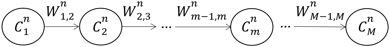
We target at application tasks whose subtasks exhibit sequential dependencies. Only after the previous subtask is completed and its output data is obtained can the next subtask begin to be computed. Thus, we model the application task as a unidirectional graph as shown in Fig. 2. Each node represents a subtask, and each edge shows the dependency between adjacent subtasks.

We use set $\mathcal{M}^{n}=\{1,2,...,M^{n}\}$ to denote the subtasks of the application task for NV_n, with the delay requirement signified by $T_{n,max}$. The computation workloads of the $m\mbox{-}th$ subtask of NV_n is $C^{n}_{m},m\in\mathcal{M}^{n}$, with the unit of CPU cycles. $W^{n}_{m-1,m}$ denotes the size of intermediate data between the $m-1\mbox{-}th$ and $m\mbox{-}th$ subtask in bits.

II-C Communication Model

The subtask assignment of an application task on different devices is represented by the following notations. In the Vehicle Tier, for each NV_n, its subtasks $C_{1}^{n},...,C_{m_{h}-1}^{n}$ are computed locally on this NV, and subtasks $C_{m_{h}}^{n},...,C_{M}^{n}$ are computed on its matched HV_h. In the RSU Tier, each NV_n’s subtasks $C^{n}_{m_{r}},...,C^{n}_{m_{r+1}-1}$ are computed on RSU_r. The last RSU_R computes subtask $C^{n}_{m_{R}},...,C^{n}_{M}$.

Based on the above establishment, for the Vehicle Tier, NV_n offloads subtasks starting from $C_{m_{h}}^{n}$. Therefore, NV_n will transmit the input data of the $m_{h}\mbox{-}th$ subtask (i.e., with the data size of $W_{m_{h}-1,m_{h}}^{n}$) to its matched HV_h. Similar to [14, 20], we adopt Orthogonal Frequency Division Multiplexing (OFDM) and Orthogonal Frequency Division Multiple Access (OFDMA) technologies for V2V and V2I communications, respectively. Each communication link occupies mutually orthogonal subbands, which exhibits strong resistance to signal interference. Assuming the bandwidth for V2V communication is $B_{V2V}$, the V2V transmission delay from NV_n to HV_h is denoted by $\tau_{n,h}$, the transmission energy consumption is $E^{t}_{n,h}$ and the power spectrum density of noise at HV is $N_{0}$. Therefore, based on Shannon capacity formula, we can obtain

$$W_{m_{h}-1,m_{h}}^{n}=\tau_{n,h}B_{V2V}\ln\left(1+\dfrac{E_{n,h}^{t}10^{-\frac{\phi_{n,h}}{10}}h_{n,h}}{\tau_{n,h}B_{V2V}N_{0}}\right),$$ (1)

where $\phi_{n,h}=63.3+17.7\lg(d_{n,h})$ [13] is the path loss between NV_n and HV_h. $d_{n,h}$ denotes the Euclidean distance between them, which can be calculated based on their positions. $h_{n,h}$ is the channel fading factor between them.

Regarding the RSU Tier, since all the subtasks will be computed collaboratively by RSUs, the NV_n needs to transmit the initial task data (i.e., the input data of the first subtask), with the data size $W^{n}_{0}$, to RSU₁. Assume that the total bandwidth of RSU₁ is $B$ and the bandwidth allocated to each V2I uplink from NV_n to RSU₁ is $b_{n}B_{0}$, where $B_{0}$ is the bandwidth of each subchannel and $b_{n}$ signifies the number of subchannels allocated to each V2I uplink. We denote the V2I transmission delay of NV_n as $\tau_{n}$, the transmission energy consumption as $E^{t}_{n}$ and the power spectrum density of noise at RSU₁ as $N_{0}$. Then we have

$$W^{n}_{0}=\tau_{n}b_{n}B_{0}\ln\left(1+\dfrac{E_{n}^{t}\phi_{n}h_{n}}{\tau_{n}b_{n}B_{0}N_{0}}\right),$$ (2)

where $\phi_{n}=d_{n}^{-\delta}$ [20] is defined as the path loss between NV_n and RSU₁, with $d_{n}$ and $\delta$ denoting the distance between them and path loss factor, respectively.

Based on (1) and (2), the expression of V2V and V2I transmission energy consumption $E_{n,h}^{t}$ and $E_{n}^{t}$ can be rewritten as follows respectively

$$E_{n,h}^{t}=\frac{B_{V2V}N_{0}\tau_{n,h}}{10^{-\frac{\phi_{n,h}}{10}}h_{n,h}}\left(e^{\frac{W_{m_{h}-1,m_{h}}^{n}}{\tau_{n,h}B_{V2V}}}-1\right),$$ (3)

$$E^{t}_{n}=\dfrac{b_{n}B_{0}N_{0}\tau_{n}}{\phi_{n}h_{n}}\left(e^{\frac{W^{n}_{0}}{\tau_{n}b_{n}B_{0}}}-1\right).$$ (4)

We model the wired transmission among RSUs as follows. Suppose that the required energy for each RSU to transmit one bit of data to the next RSU through wired link is $E_{0}$ and the delay for transmitting one bit is $\tau_{0}$. Then the energy consumption for RSU_r to transmit the intermediate data of NV_n to RSU_r+1 can be expressed by $E^{t}_{r,n}=E_{0}W^{n}_{m_{r+1}-1,m_{r+1}}$ and the corresponding data transmission delay is $\tau_{r,n}=\tau_{0}W^{n}_{m_{r+1}-1,m_{r+1}}$.

II-D Computation Model

We adopt a general CPU computation model so that the strategy in this paper is also applicable to other more specific scenarios. The CPU frequency $f$ (also known as CPU clock speed) is defined as the number of CPU cycles that can be processed per second. For a specific $f$, the computing power can be expressed by $\kappa f^{3}$, where $\kappa$ is the energy efficiency coefficient of the chip, a constant related to hardware [6]. When the processor computes a task with the workloads of $C$ CPU cycles, the computation delay is $C/f$. Hence the computation energy consumption is $\kappa Cf^{2}$. We denote the $\kappa$ of NV_n, HV_h, and RSU_r as $\kappa_{n}$, $\kappa_{h}$, and $\kappa_{r}$, respectively. The maximal CPU frequency (i.e., maximal computing resources) of NV_n, IV_i, HV_h, and RSU_r are $F_{n}$, $F_{i}$, $F_{h}$, and $F_{r}$, respectively. In order to save energy, the working frequency of each device will be optimized instead of directly using the maximum.

In the Vehicle Tier, the CPU frequency allocated by each pair of NV_n and HV_h when computing the subtask $C_{m}^{n}$ are denoted by $f^{n}_{m}$ and $f^{h}_{m}$, respectively. According to the subtask assignment representation in Section II-C, the computation delay of each subtask, symbolized by $\tau_{n,m}^{c}$, can be expressed as $\tau_{n,m}^{c}=\frac{C_{m}^{n}}{f^{n}_{m}},1\leq m\leq m_{h}-1$ and $\tau_{n,m}^{c}=\frac{C_{m}^{n}}{f^{h}_{m}},m_{h}\leq m\leq M^{n}$. The energy consumption for computing each subtask can be written as $E_{n,m}^{c}=\kappa_{n}C_{m}^{n}\left(f^{n}_{m}\right)^{2},1\leq m\leq m_{h}-1$ and $E_{n,m}^{c}=\kappa_{h}C_{m}^{n}\left(f^{h}_{m}\right)^{2},m_{h}\leq m\leq M^{n}$. In the RSU Tier, we denote the CPU frequency allocated by RSU_r to compute the subtask $C^{n}_{m}$ of NV_n as $f^{r}_{n,m}$. Similarly, the computation delay and energy consumption of each subtask of NV_n are $\tau^{c}_{n,m}=\frac{C_{m}^{n}}{f^{r}_{n,m}}$ and $E^{c}_{n,m}=\kappa_{r}C_{m}^{n}\left(f^{r}_{n,m}\right)^{2},\forall n\in\mathcal{N},m_{r}\leq m\leq m_{r+1}-1,\forall r\in\mathcal{R}$, respectively.

III Tier-1: Collaborative Computation between NV and HV in the Vehicle Tier

In this section, we elaborate the study of the Vehicle Tier. We first present the NV-HV matching algorithm, followed by the formulation of the subproblem that minimizes vehicle energy consumption under the constraints of task delay requirements and computing resources of vehicles. Subsequently, we discuss the solution to this subproblem.

III-A NV-HV Matching

Consider the scenario where initial system consists of $N$ NV and $I$ IV. After the matching process, the IV that are ultimately selected to serve as helpers for NV will become HV. In this subsection, we introduce the proposed NV-HV matching algorithm, which aims to match as many NV as possible with qualified HV in the Vehicle Tier.

We consider the positions and velocities of NVs and IVs, the computational workloads and delay requirements of each NV’s task, as well as the maximum computing resources available for each IV similar to [30]. The maximum V2V communication range is denoted by $D_{V2V}$. The matching algorithm consists of the following two parts:

(1) Candidate NV-IV Matching Identification: Only the NV-IV pair that simultaneously satisfies the following two conditions can be considered as a candidate match:

• V2V Communication Range Condition: The real-time distance between the two vehicles is less than $D_{V2V}$ or the distance is equal to $D_{V2V}$, but the vehicle positioned behind is driving at a higher speed than the one in front, implying that the two vehicles are approaching each other. Note that, to prevent communication interruption, the extreme case where the distance is equal to $D_{V2V}$ while the speeds of the two vehicles are identical is considered not to meet this condition.

• IV Computing Resource Condition: When the IV utilizes its maximum computing resources to process the NV’s task, the corresponding computation delay must be shorter than the delay requirement of this task.

Through this process, we obtain all potential NV-IV matches. Note that by this point, each NV may have one, multiple, or no candidate IV.

(2) Maximum Matching for NVs: We resort to the Hungarian algorithm [31] to perform the maximum matching for NVs based on the current set of candidate NV-IV matches. The selected IVs in the final matching are promoted to HVs. In this manner, we maximize the number of NV that can find suitable HV under the given system conditions in the Vehicle Tier. Subsequently, we further optimize the task offloading decision and the allocation strategies for communication and computation resources of each NV-HV pair.

III-B Problem Formulation of Vehicle Tier

After the determination of NV-HV pairs, in this subsection, we formulate the subproblem to jointly optimize task offloading decision, V2V transmission delay and computation resource allocation. The objective is to minimize the weighted sum energy consumption of vehicles while ensuring the delay requirements of NVs’ application tasks can be met. The optimization problem $\mathcal{P}_{1}$ of Tier-1 is formulated as follows.

$\mathcal{P}_{1}:$ Collaborative computation of vehicles

$$\min_{\begin{subarray}{c}\mathbf{m_{h}},\mathbf{\tau_{n,h}},\\ \mathbf{f_{m}^{V}}\end{subarray}} \sum_{h=1}^{H}\left[w_{n}\left(E_{n,h}^{t}+\sum_{m=1}^{m_{h}-1}E_{n,m}^{c}\right)+w_{h}\sum_{m=m_{h}}^{M^{n}}E_{n,m}^{c}\right]$$

s.t. $$1\leq m_{h}\leq M^{n},\forall h\in\mathcal{H},$$ (5a)

$$\sum_{m=1}^{M^{n}}\tau_{n,m}^{c}+\tau_{n,h}\leq T_{n,max},\forall h\in\mathcal{H},$$ (5b)

$$\tau_{n,h}\geq 0,\forall h\in\mathcal{H},$$ (5c)

$$0\leq f^{n}_{m}\leq F_{n},m=1,...,m_{h}-1,\forall h\in\mathcal{H},$$ (5d)

$$0\leq f^{h}_{m}\leq F_{h},m=m_{h},...,M^{n},\forall h\in\mathcal{H}.$$ (5e)

In the objective function, the first two terms are the V2V data transmission energy and the computation energy of the first $m_{h}-1$ subtasks consumed by each NV, respectively. HV’s energy consumption for computing the remaining subtasks is represented by the last term. The $w_{n}$ and $w_{h}$ are the weights of NV_n and HV_h, respectively. Note that not all NVs can be matched in the Vehicle Tier. Therefore, we use the index $n$ of HV to correspond to each NV-HV pair.

Regarding the optimization variables, set $\mathbf{m_{h}}=\{m_{h}|h\in\mathcal{H}\}$ encompasses the index of the first subtask computed on each HV, indicating the offloading decision for each pair. The V2V data transmission delays are denoted by $\mathbf{\tau_{n,h}}=\{\tau_{n,h}|h\in\mathcal{H}\}$. Set $\mathbf{f_{m}^{V}}$ is the union of $\left\{f^{n}_{m}|m=1,...,m_{h}-1\right\}$ and $\left\{f^{h}_{m}|m=m_{h},...,M^{n}\right\}$, $\forall h\in\mathcal{H}$, including the computing resources allocated by the two types of vehicles to compute each subtask.

In terms of the constraints, (5a) limits the range of each $m_{h}$. The total execution delay does not exceed the required delay of each application is guaranteed by (5b). Constraint (5c) ensures the nonnegativity of the transmission delay. The allocated computing resources by the two types of vehicles to each subtask will not be greater than their maximal computing resources are guaranteed by (5d) and (5e).

III-C Problem Solving

To solve this MINLP problem, our strategy is to decompose $\mathcal{P}_{1}$ into two subproblems. In the first subproblem $\mathcal{P}_{1-1}$, we initially fix the integer variable $m_{h}$ and then optimize the remaining two types of continuous variables. In the second subproblem $\mathcal{P}_{1-2}$, the optimal $m_{h}^{*}$ for each NV-HV pair is determined via the exhaustive searching.

For the convenience of presentation, we make the following definitions for each pair:

$$f^{V}_{m}\triangleq\begin{cases}f^{n}_{m},&m=1,\ldots,m_{h}-1,\\ f^{h}_{m},&m=m_{h},\ldots,M^{n},\end{cases}$$ (6)

$$F_{V}\triangleq\begin{cases}F_{n},&m=1,\ldots,m_{h}-1,\\ F_{h},&m=m_{h},\ldots,M^{n}.\end{cases}$$ (7)

Through the above definitions, we combine equations (5d) and (5e) into

$$0\leq f^{V}_{m}\leq F_{V},m=1,...,M^{n}.$$ (8)

Proposition 1: $\mathcal{P}_{1-1}$ is a convex optimization problem.

Proof: Regarding the objective function, the second-order derivative of the first term $w_{n}E_{n,h}^{t}$ w.r.t. $\tau_{n,h}$ is always greater than zero, indicating the convexity for $\tau_{n,h}$. The second and third terms are convex functions w.r.t. $f^{n}_{m}$ and $f^{h}_{m}$, respectively. Since the objective function is the sum of convex functions, it is also convex. As for the constraints, the function $\frac{C_{m}^{n}}{f^{V}_{m}}$ in the first term of constraint (5b) is convex with $f^{V}_{m}$ and constraint (8) are affine functions of $f^{V}_{m}$ that are also convex. Additionally, the constraints (5b) and (5c) are all affine and convex with $\tau_{n,h}$. This completes the proof. $\hfill\blacksquare$

The convexity of this problem indicates that we can directly derive globally optimal solution that meets the delay requirements while minimizing vehicle energy consumption. Coupled with the satisfaction of Slater’s condition, it can be efficiently solved by the Karush-Kuhn-Tucker (KKT) conditions algorithm with low complexity. The fast execution speed of algorithm is well suited for real-time decision-making demand in highly dynamic traffic environment. Then we can derive the optimal solutions of $\tau_{n,h}$ and $f^{V}_{m}$ as presented in the following.

Lemma 1: The optimal V2V transmission delay for each NV-HV pair is:

$$\tau^{*}_{n,h}=\frac{W_{m_{h}-1,m_{h}}^{n}}{B_{V2V}\left[{W_{0}\left({\frac{\frac{10^{-\frac{\phi_{n,h}}{10}}h_{n,h}\lambda}{w_{n}N_{0}B_{V2V}}-1}{e}}\right)+1}\right]}.$$ (9)

Proof: The KKT conditions formulas of the problem $\mathcal{P}_{1-1}$ are listed as following:

Constraints (5b), (5c) and (8),

$$\lambda\left(\sum_{m=1}^{M^{n}}\frac{C_{m}^{n}}{f^{V}_{m}}+\tau_{n,h}-T_{n,max}\right)=0,$$ (10a)

$$\eta\tau_{n,h}=0,$$ (10b)

$$\mu_{m}f^{V}_{m}=0,m=1,\ldots,M^{n},$$ (10c)

$$\nu_{m}\left(f^{V}_{m}-F_{V}\right)=0,m=1,\ldots,M^{n},$$ (10d)

$$\frac{w_{n}B_{V2V}N_{0}}{10^{-\frac{\phi_{n,h}}{10}}h_{n,h}}\left(e^{\frac{W_{m_{h}-1,m_{h}}^{n}}{\tau_{n,h}B_{V2V}}}-1\right)$$

$$-\frac{w_{n}N_{0}W_{m_{h}-1,m_{h}}^{n}e^{\frac{W_{m_{h}-1,m_{h}}^{n}}{\tau_{n,h}B_{V2V}}}}{10^{-\frac{\phi_{n,h}}{10}}h_{n,h}\tau_{n,h}}+\lambda-\eta=0,\hskip 25.6073pt$$ (10e)

$$2w_{n}\kappa_{n}C_{m}^{n}f^{V}_{m}-\lambda\frac{C_{m}^{n}}{\left({f^{V}_{m}}\right)^{2}}-\mu_{m}+\nu_{m}=0,$$

$$m=1,\ldots,m_{h}-1,$$ (10f)

$$2w_{h}\kappa_{h}C_{m}^{n}f^{V}_{m}-\lambda\frac{C_{m}^{n}}{\left({f^{V}_{m}}\right)^{2}}-\mu_{m}+\nu_{m}=0,$$

$$m=m_{h},\ldots,M^{n}.$$ (10g)

where $\lambda$, $\eta$, $\mu_{m}$ and $\nu_{m}$ are the nonnegative Lagrange multipliers associated with the constraint (5b), (5c), $f^{V}_{m}\geq 0$ and $f^{V}_{m}\leq F_{V}$, respectively.

We have $\tau_{n,h}>0$ to guarantee the rationality. Therefore, we have $\eta=0$ based on (10b). We can define $d\triangleq\frac{W_{m_{h}-1,m_{h}}^{n}}{B_{V2V}\tau_{n,h}}$. Hence, (10e) can be expressed as

$$(d-1)e^{d-1}=\frac{\frac{10^{-\frac{\phi_{n,h}}{10}}h_{n,h}\lambda}{w_{n}N_{0}B_{V2V}}-1}{e}.$$ (11)

In order to obtain the optimal expression of $\tau_{n,h}$, we leverage the function $W_{0}(x)$ whose definition is given in TABLE I. Since $d>0$, we have $d-1>-1$. Therefore, we can obtain

$$d=W_{0}\left(\frac{\frac{10^{-\frac{\phi_{n,h}}{10}}h_{n,h}\lambda}{w_{n}N_{0}B_{V2V}}-1}{e}\right)+1.$$ (12)

Then we substitute the defined expression of $d$ into (12) and we can finally get the optimal solution as given in (9).$\hfill\blacksquare$

Lemma 2: The optimal allocation of computing resource for each subtask by NV and HV is:

$${f^{V}_{m}}^{*}=\min\left({\left({\frac{\lambda}{2w_{g(m)}\kappa_{g(m)}}}\right)^{\frac{1}{3}},F_{V}}\right),m=1,\ldots,M^{n},$$ (13)

where $g(m)$ is $n$ when $1\leq m\leq m_{h}-1$ and $h$ when $m_{h}\leq m\leq M^{n}$. The optimal value of $\lambda$ can be easily found using the bisection searching method.

Proof: According to the function $\frac{C_{m}^{n}}{f^{V}_{m}}$ in the first term of (5b), we should restrict $f^{V}_{m}\neq 0$, and we have $\mu_{m}=0$ based on (10c). We focus on the solution of $\left\{f^{V}_{m}|m=1,\ldots,m_{h}-1\right\}$ and optimal $\left\{f^{V}_{m}|m=m_{h},\ldots,M^{n}\right\}$ can be obtained similarly.

For $m=1,\ldots,m_{h}-1$, when $0<f^{V}_{m}<F_{V}$, then $\nu_{m}=0$ according to (10d). Thus, we can rewrite the (10f) as

$$2w_{n}\kappa_{n}C_{m}^{n}f^{V}_{m}=\lambda\frac{C_{m}^{n}}{\left({f^{V}_{m}}\right)^{2}}.$$ (14)

The computing resources allocated to each subtask becomes

$$f^{V}_{m}=\left(\frac{\lambda}{2w_{n}\kappa_{n}}\right)^{\frac{1}{3}}.$$ (15)

When $f^{V}_{m}=F_{V}$, then $\nu_{m}\geq 0$. Hence (10f) is rewritten as

$$2w_{n}\kappa_{n}C_{m}^{n}f^{V}_{m}+\nu_{m}=\lambda\frac{C_{m}^{n}}{\left({f^{V}_{m}}\right)^{2}},$$ (16)

where $f^{V}_{m}$ can be replaced by $F_{V}$. Assuming that for $m\in\left\{1,\ldots,m_{h}-1\right\}$, some of them have the expression of $f^{V}_{m}$ satisfying (15) while some have $f^{V}_{m}=F_{V}$. This means that equations (14) and (16) hold simultaneously. We can obtain the following inequality chain

$$\lambda \overset{\text{(a)}}{=}2w_{n}\kappa_{n}\left(F_{V}\right)^{3}+\nu_{m}\frac{\left(F_{V}\right)^{2}}{C_{m}^{n}}$$

$$\overset{\text{(b)}}{\geq}2w_{n}\kappa_{n}\left(F_{V}\right)^{3}$$

$$\overset{\text{(c)}}{>}2w_{n}\kappa_{n}\left(f^{V}_{m}\right)^{3}$$

$$\overset{\text{(d)}}{=}\lambda.$$ (17)

(a) is transformed from (16) and the inequality (b) holds due to $\nu_{m}\geq 0$. When $0<f^{V}_{m}<F_{V}$, we have (c), which is also the expression of $\lambda$. We can find that there is a contradiction. Thus, for the $m\in\left\{1,\ldots,m_{h}-1\right\}$, all the $f^{V}_{m}$ will follow one of these two formulas, i.e., (15) or $f^{V}_{m}=F_{V}$.

Then we present under what circumstances which one should be followed. Obviously, the upper bound for the value of $\lambda$ is $2w_{n}\kappa_{n}\left(F_{V}\right)^{3}$. Suppose that when $\lambda<2w_{n}\kappa_{n}\left(F_{V}\right)^{3}$, the $f^{V}_{m}=F_{V},m=1,\ldots,m_{h}-1$ is followed. In this case, $\nu_{m}\geq 0$ and still $\mu_{m}=0$. According to (10f), we have

$$\lambda =2w_{n}\kappa_{n}\left(F_{V}\right)^{3}+\nu_{m}\frac{\left(F_{V}\right)^{2}}{C_{m}^{n}}$$

$$\geq 2w_{n}\kappa_{n}\left(F_{V}\right)^{3}.$$ (18)

There is a contradiction. Therefore, when $\lambda<2w_{n}\kappa_{n}\left(F_{V}\right)^{3}$, the optimal solution of $f^{V}_{m}$ should be (15). When $\lambda\geq 2w_{n}\kappa_{n}\left(F_{V}\right)^{3}$, if (15) is followed, we have $f^{V}_{m}\geq F_{V}$. This violates the constraint (8). Thus, the optimal solution is $f^{V}_{m}=F_{V}$ in this case. We merge the optimal expressions of $\left\{f^{V}_{m}|m=1,\ldots,M^{n}\right\}$ into (13).

By this point, we express the optimal transmission delay and computing resource allocation policy as the functions of $\lambda$. Then the condition that the $\lambda^{*}$ satisfies and the method for obtaining it are given as follows. In the objective function of $\mathcal{P}_{1-1}$, the first term is monotonically decreasing with $\tau_{n,h}$ when $\tau_{n,h}>0$ (this can be easily proved by second-order derivative) and the rest two terms are monotonically increasing with $f^{n}_{m}$ and $f^{h}_{m}$, respectively. Based on (9), $\tau_{n,h}^{*}$ is monotonically decreasing with $\lambda$, while (13) indicating that ${f^{V}_{m}}^{*}$ are monotonically nondecreasing with $\lambda$. Therefore, the objective function is monotonically increasing with $\lambda$. To minimize the function value, $\lambda$ should be as small as possible.

As for the constraint (5b), the function in the left-hand side is monotonically decreasing with $\lambda$. Thus, we only need to find the $\lambda$ that activates the inequality (5b). Due to the monotonicity, this value can be found using the bisection searching method. $\hfill\blacksquare$

III-D Complexity Analysis

The complexity of the NV-HV matching algorithm consists of two parts: candidate NV-IV matching identification and maximum matching for NVs. The first part needs to iterate through all NV-IV pairs to verify whether they meet V2V communication range and IV computing resource conditions. Consequently, the complexity of this part is $\mathcal{O}\left(NI\right)$. The method for maximum matching is to search for augmenting paths. For each NV, in the worst case, it may need to traverse all edges (i.e., the candidate matches in the adjacency list obtained from the first part). Hence, the complexity of the second part is $\mathcal{O}\left(N^{2}I\right)$. The overall worst-case complexity of the matching algorithm is $\mathcal{O}\left(NI+N^{2}I\right)\approx\mathcal{O}\left(N^{2}I\right)$. When the adjacency list is sparse, the complexity will be significantly reduced. Obtaining the optimal task offloading decision for each matched NV requires traversing its subtasks, resulting in a complexity of $\mathcal{O}\left(H\overline{M}\right)$, where $\overline{M}$ represents the average number of subtasks for each application. Note that the reason for using the number of HVs $H$ here is that it is equivalent to the number of NVs successfully matched in the Vehicle Tier. The optimal V2V transmission delay and computing resource allocation strategy can be directly derived by substituting the known parameters into the optimal solution expressions, which belong to constant time complexity. Consequently, the overall complexity of the method in the Vehicle Tier is $\mathcal{O}\left(N^{2}I+H\overline{M}\right)$.

IV Tier-2: Collaborative Computation in the RSU Tier

In this section, the cooperation among RSUs to compute the application tasks for NVs is investigated. The NVs that fail to be successfully matched with a suitable HV in the Vehicle Tier will offload their tasks to RSU. After that, each RSU will compute several subtasks and transmit the intermediate data to the next RSU for further computation.

IV-A Problem Formulation of RSU Tier

Compared with Tier-1, each RSU will serve multiple NVs, and thus we further address the multi-access issues for bandwidth and computing resource allocation. In this tier, the NVs being served are those that failed to be matched in the Vehicle Tier, symbolized by the set $\mathcal{N}^{\prime}$ with a total number of $N^{\prime}$. In this work, we consider that RSUs can compute multiple tasks in parallel and optimize the multi-access allocation of their computing resources with the assumption that tasks can begin computation immediately upon arrival. We formulate the problem $\mathcal{P}_{2}$ of the RSU Tier as

$\mathcal{P}_{2}$: Collaborative computation of RSUs

$$\min_{\begin{subarray}{c}\mathbf{m^{n}_{r}},\mathbf{\tau_{n}},\\ \mathbf{f^{r}_{n,m^{n}}},\mathbf{b_{n}}\end{subarray}}\hskip 8.5359pt \sum^{N^{\prime}}_{n=1}\left[w_{n}E^{t}_{n}+\sum_{r=1}^{R}w_{r}\left(E^{t}_{r,n}+\sum_{m^{n}=m_{r}^{n}}^{m_{r+1}^{n}-1}E^{c}_{n,m}\right)\right]$$

s.t. $$1\leq m_{1}^{n}\leq\cdots\leq m_{r}^{n}\leq m_{r+1}^{n}\leq\cdots\leq M^{n}+1,$$

$$n\in\mathcal{N^{\prime}},r\in\mathcal{R},$$ (19a)

$$\sum_{q=1}^{Q^{n}}\frac{D^{n}_{q}}{R_{n}}+\tau_{n}+\sum_{r=1}^{R}\sum_{m^{n}=m^{n}_{r}}^{m^{n}_{r+1}-1}\tau^{c}_{n,m}+\sum_{r=1}^{R-1}\tau_{r,n}$$

$$\leq T_{n,max},n\in\mathcal{N^{\prime}},$$ (19b)

$$\sum_{q=1}^{Q^{n}}\frac{D^{n}_{q}}{R_{n}}+\tau_{n}\leq\frac{L-S_{n}}{v_{n}},n\in\mathcal{N^{\prime}},$$ (19c)

$$0\leq\tau_{n}\leq\tau_{max},n\in\mathcal{N^{\prime}},$$ (19d)

$$\sum_{n=1}^{N^{\prime}}b_{n}\leq b,b_{n}\in\mathcal{I}_{+},$$ (19e)

$$0\leq\sum_{n=1}^{N^{\prime}}f^{r}_{n,m^{n}}\leq F_{r},r\in\mathcal{R}.$$ (19f)

The objective function consists of the energy consumption of data transmission from NVs to RSU₁, data transmission from each RSU_r to the next RSU, and computation on RSUs, respectively. Note that the second term of the RSU that computes the last subtask of NV_n is zero since it does not need to transmit data. $w_{n}$ and $w_{r}$ are the weights of NV_n and RSU_r. Then the objective function is the summation of the energy consumption for each NV_n.

The optimization variables are categorized into four sets. The first set $\mathbf{m_{r}^{n}}=\left\{m^{n}_{r}|n\in\mathcal{N},r\in\mathcal{R}\right\}$ consists of the task offloading decisions for all NVs’ application tasks. The second set $\mathbf{\tau_{n}}=\left\{\tau_{n}|n\in\mathcal{N}\right\}$ comprises the data transmission delays from each NV_n to RSU₁. The third set $\mathbf{f^{r}_{n,m^{n}}}=\left\{f^{r}_{n,m^{n}}|m^{n}\in\mathcal{M}^{n},n\in\mathcal{N},r\in\mathcal{R}\right\}$ contains the computing resource allocation policy for each subtask of each NV. Lastly, the fourth set $\mathbf{b_{n}}=\left\{b_{n}|n\in\mathcal{N}\right\}$ includes the number of subchannels allocated to each V2I link.

As for the constraints, (19a) ensures the relationship and the range of task offloading decisions (i.e., $m^{n}_{r}$) for each NV_n. In (19b), the first term is the communication setup delay between each NV_n and RSU₁, where $Q^{n}$ signifies the total number of the communication setup messages of NV_n, $D^{n}_{q}$ denotes the data size of the $q\mbox{-}th$ setup message of NV_n, and $R_{n}$ is the data rate of the communication link dedicated for the transmission of the NV_n’s setup messages. The following two terms are the V2I data transmission delay and the sum of computation delay on RSUs, respectively. The data transmission delays from an RSU to the next one are summed in the last term. Hence (19b) guarantees the total execution delay of the NV_n’s application task will not exceed its delay requirement. (19c) is related to the mobility of NVs, where $L$ is the length of RSU₁’s service range, $S_{n}$ denotes the distance from the starting point of service range to the current position of NV_n. Thus, it guarantees that NV_n completes communication setup and data uploading with RSU₁ before leaving its service range. (19d) ensures the data transmission delays are nonnegative and not greater than a tolerant threshold $\tau_{max}$. The sum of subchannels allocated to each V2I link should not exceed the total available number of subchannels $b$ is guaranteed by (19e), where $\mathcal{I}_{+}$ is the set of positive integers. (19f) ensures the summation of the allocated computation resources should not exceed the available resources of the corresponding RSU.

Remark: In constraint (19a), $m^{n}_{r}=m^{n}_{r+1}$ means the RSU_r is not assigned any subtask of NV_n and only needs to transmit data to RSU_r+1. These RSUs are referred to as TYPE 1 RSUs. When $m^{n}_{r}=M^{n}+1$, it means previous RSUs have completed all the subtasks of NV_n. Hence the RSU_r will do nothing for NV_n. We call them TYPE 2 RSUs. Therefore, in the objective function and constraint (19b), the computation delay and energy consumption of TYPE 1 RSUs are zero, while all the delay and energy consumption for both of transmission and computation of TYPE 2 RSUs are zero.

IV-B Solutions to Allocation Policies of Communication and Computation Resources

Similar to $\mathcal{P}_{1}$, we decompose the problem $\mathcal{P}_{2}$ into two subproblems. In subproblem $\mathcal{P}_{2-1}$, we begin by fixing the integer variable set $\mathbf{m_{r}^{n}}$ and then optimize the remaining variables. Subsequently, the optimal values of each $m^{n}_{r}$ can be obtained in the second subproblem $\mathcal{P}_{2-2}$. This subsection presents the solving process for continuous variables.

For notational simplicity, we make the following definition:

$$f_{n,m^{n}}\triangleq f^{r}_{n,m^{n}},m^{n}=m^{n}_{r},\ldots,m^{n}_{r+1}-1.$$ (20)

For the RSU that computes the last subtask of NV_n, $m^{n}_{r+1}-1=M^{n}$. Based on the above definition, we can rewrite the third term in (19b) by merging the computation delay of each RSU to compute subtasks for NV_n into $\sum_{m^{n}=1}^{M^{n}}\frac{C^{n}_{m}}{f_{n,m^{n}}}$. We have another definition as

$$F\triangleq F_{r},m^{n}=m^{n}_{r},\ldots,m^{n}_{r+1}-1.$$ (21)

According to the above definition, (19f) can be transformed into the following constraint:

$$0\leq\sum_{n=1}^{N^{\prime}}f_{n,m^{n}}\leq F,m^{n}\in\mathcal{M}^{n}.$$ (22)

To enhance the practicality of the problem, bandwidth allocation involves allocating a specific number of subchannels to each V2I uplink. However, directly obtaining the optimal integer set $\mathbf{b_{n}}$ is an NP-Hard problem with high complexity. Therefore, a two-step strategy is proposed. Initially, the bandwidth allocated to each V2I link is treated as a continuous variable to find the optimal solution. Subsequently, the method of adjacent integer point searching is utilized to obtain near-optimal solutions for the integer set $\mathbf{b_{n}}$. Consequently, the variable $b_{n}B_{0}$ in the problem is first converted into $B_{n}$, which represents the bandwidth allocated to each V2I link in continuous value. The constraint (19e) should be then transformed into the following constraints:

$$\sum_{n=1}^{N^{\prime}}B_{n}\leq B,$$ (23a)

$$B_{n}\geq 0,n\in\mathcal{N^{\prime}}.$$ (23b)

Proposition 2: $\mathcal{P}_{2-1}$ is a convex optimization problem.

Proof: As for the objective function, the Hessian matrix of the first term $w_{n}E^{t}_{n}$ w.r.t. $\tau_{n}$ and $B_{n}$ is positive-definite, proving its convexity. The second term is determined when offloading decisions are fixed in $\mathcal{P}_{2-1}$. The third term is convex with $f^{r}_{n,m^{n}}$. Thus, the objective function is convex since it is the sum of convex functions. Regarding the constraints, function $\frac{C^{n}_{m}}{f_{n,m^{n}}}$ in (19b) is convex with $f_{n,m^{n}}$ and (22) are affine functions of $f_{n,m^{n}}$ that are also convex. (19b), (19c), and (19d) are all affine and convex with $\tau_{n}$. (23) are convex with $B_{n}$. This completes the proof. $\hfill\blacksquare$

$\mathcal{P}_{2-1}$ is an intricate problem incorporating three sets of optimization variables. However, the convexity of the problem inspires us to propose an iterative optimization-based method to obtain the optimal continuous solution of V2I transmission delay and bandwidth allocation policy. On this basis, we further adapt the method to deal with the subchannel allocation. Due to space limitation, we will not repeat the mathematical derivation similar to Tier-1 but focus our analysis on the different parts. We can obtain the optimal solutions of the continuous variables as follows.

Lemma 3: The optimal solutions of the V2I transmission delay, V2I bandwidth allocation, and computing resources allocation policy are given by

$$\tau^{*}_{n}=\frac{W^{n}_{0}}{B_{n}\left[{W_{0}\left({\frac{\frac{\lambda_{n}\phi_{n}h_{n}}{w_{n}N_{0}B_{n}}-1}{e}}\right)+1}\right]},n\in\mathcal{N^{\prime}},$$ (24a)

$$B^{*}_{n}=\frac{W^{n}_{0}}{\tau_{n}\left[{W_{0}\left({\frac{\frac{\xi\phi_{n}h_{n}}{w_{n}N_{0}\tau_{n}}-1}{e}}\right)+1}\right]},n\in\mathcal{N^{\prime}},$$ (24b)

$${f^{r}_{n,m^{n}}}^{*}=\min\left({\left({\frac{\lambda_{n}}{2w_{r}\kappa_{r}}}\right)^{\frac{1}{3}},F_{r}}\right),$$

$$m^{n}=m^{n}_{r},\ldots,m^{n}_{r+1}-1,n\in\mathcal{N^{\prime}},r\in\mathcal{R},$$ (24c)

where the $\lambda_{n}$ and $\xi$ are nonnegative Lagrange multipliers associated with the constraint (19b) and (23a), respectively.

Proof: The proof is similar to lemma 1 and lemma 2. $\hfill\blacksquare$

Regarding the solution of $\tau_{n}$, three other Lagrange multipliers $\theta_{n},\eta_{n}$, and $\alpha_{n}$ are involved, associated with (19c), $\tau_{n}\geq 0$, and $\tau_{n}\leq\tau_{max}$, respectively. Due to the necessary V2I data transmission, $\tau_{n}$ must be greater than 0. Hence $\eta_{n}=0$. Both the constraint (19c) and $\tau_{n}\leq\tau_{max}$ guarantee that the $\tau_{n}$ will not exceed a known value. Thus, after we get the solution through (24a), we only need to consider the minimum of these three values. Following the similar analysis of Tier-1, the optimal $\lambda_{n}$ for each NV_n is the one that activates the constraint (19b). Then we can obtain the optimal $\tau^{*}_{n}$ and ${f^{r}_{n,m^{n}}}^{*}$.

In order to get the optimal $B^{*}_{n}$ for each NV_n, we conduct the following analysis. The optimal $B^{*}_{n}$ is only achieved when the total bandwidth $B$ is fully allocated. This means the constraint (23a) is activated. Because as long as there is still bandwidth not allocated, when it is allocated to any one or several V2I links, the transmission energy consumption of the corresponding links will be further reduced. Hence we need to find a $\xi$ such that $\sum_{n=1}^{N^{\prime}}B_{n}=B$. According to (24b), the left-hand side part monotonically decreases with $\xi$. Therefore, finding such $\xi$ is a zero point searching problem for a monotone function.

From (24a) and (24b), we observe that the optimal solution expressions of the $\tau^{*}_{n}$ and $B^{*}_{n}$ are very similar and inclusive of each other. To address this dilemma, we use an iterative optimization method depicted as the following. To start the iteration, we adopt the equal allocation strategy to initialize the values of the set $\left\{B_{n}|n\in\mathcal{N^{\prime}}\right\}$. Based on this, the optimization of set $\mathbf{\tau_{n}}$ can be implemented through (24a). Then according to the once-optimized $\tau_{n}$, we can get the once-optimized $B_{n}$. Subsequently, the $h_{n}$ of each V2I uplink can be updated. Next, we repeat the above steps until the optimizing process converges. We set an accuracy for the iteration termination. When the difference between the variables of current round and previous round is less than the threshold, we terminate the iterative optimization process.

IV-C Solutions to Subchannel Allocation and Offloading Decisions

By this point, we have completed the optimization of all continuous variables in $\mathcal{P}_{2-1}$. In this subsection, we will present the solving process of integer variables.

We propose the adjacent integer point searching method to solve the subchannel allocation problem. A set $\left\{B_{n}|n\in\mathcal{N^{\prime}}\right\}$ is regarded as a point in an $N$-dimensional space, with each $B_{n}$ as the coordinate value. Assume the optimal continuous solution set $\left\{B^{*}_{n}|n\in\mathcal{N^{\prime}}\right\}$ we have obtained corresponds to the point $B^{*}$. Then we search for its adjacent points whose coordinates are integers (by rounding each $B_{n}$ up and down) on the hyperplane $\sum_{n=1}^{N^{\prime}}B_{n}=B$. Since the objective function of $\mathcal{P}_{2-1}$ is convex with $B_{n}$ and the weights of each $B_{n}$ in the hyperplane expression are equal, by comparing the objective function values corresponding to those integer points, we can find the near-optimal integer solution set $\mathbf{b_{n}}$. Assuming that the number of NVs served by RSUs, denoted by $N^{\prime}$, is at least two. Since an even number of coordinate values of $B^{*}$ will be rounded up or down in pairs to ensure their sum equals $B$, the number of adjacent points satisfying the above conditions can be expressed as $\sum_{k=2}^{K}\binom{N^{\prime}}{k}=2^{N^{\prime}-1}-1$, where $K$ is the largest even number less than $N^{\prime}$. Therefore, the complexity of this method is $\mathcal{O}(2^{N^{\prime}})$. In the above method, the bandwidth of each subchannel is 1 unit. If we want to change the granularity of bandwidth division, for example, to $B_{0}$ units, we only need to search the adjacent points whose coordinates are the multiples of $B_{0}$.

The optimal integer set $\mathbf{m^{n^{*}}_{r}}$ can be obtained through solving the subproblem $\mathcal{P}_{2-2}$. We will analyze the complexity of the enumerating method based on the practical situation. We consider $200$ m as the average service range of RSU [32]. Since our target application scenario is a regular highway, we take the example of vehicle speed as 100 km/h (i.e., 27.8 m/s). Hence the time for each vehicle to pass through the service range of an RSU is approximately 7.2 s, much greater than the delay requirement of aimed applications (i.e., hundreds of milliseconds which is around human average reaction time). Considering spatial utilization efficiency, a reasonable scenario is that the task of an NV should be collaboratively computed by 2 to 3 nearby RSUs. When the number of RSUs is 2, then for each NV_n, only one integer variable $m^{n}_{2}$ needs to be optimized. Assuming that the average number of subtasks within one application is $\overline{M}$. The complexity of the enumerating method in this case is $\mathcal{O}\left(\overline{M}N^{\prime}\right)$. If the number of RSUs is 3, there will be 2 integer variables (i.e., $m^{n}_{2}$ and $m^{n}_{3}$) for each NV. The optimal value can be found through a two-layer loop. In the inner loop, we fix $m^{n}_{2}$ and traverse the value of $m^{n}_{3}$ from $m^{n}_{2}$ to $M^{n}+1$. In the outer loop, we traverse the value of $m^{n}_{2}$ from 1 to $M^{n}+1$. The complexity of this scenario is $\mathcal{O}\left(\overline{M}^{2}N^{\prime}\right)$.

V Simulations

In this section, we conduct extensive experiments to evaluate the performance of the proposed method and compare it with other baseline methods. Furthermore, we analyze the impact of various system parameters on the performance of the proposed method.

Without losing generality, the priority weight of each device is unified as 1. Regarding the application with sequential subtasks, we adopt the image classification application[33] with eight-layer DNN as an example. These concatenated layers can be regarded as eight sequential subtasks. The input data size of each subtask is the amount of data that each network layer needs to process. The computational workload for each subtask is the number of CPU cycles required by each layer to process its input data. This can be estimated based on parameters such as the dimensions of the input feature maps and the output feature maps, the size of the convolution kernel, and the size of the pooling windows, etc. To evaluate the applicability and robustness of the proposed method with diverse tasks, similar to [27], the input data size and the computational workload of each subtask follow the uniform distribution within the range of $[1,20]$ Mb and $[1,1000]\times 10^{6}$ CPU cycles, respectively. The power spectral density is set to $N_{0}=-140$ dBW/Hz. The default delay requirement for each application is initialized as $0.2$ s near the average human reaction time.

V-A Experiment for Vehicle Tier

In this subsection, we present the experimental configurations and results of the vehicle tier. We consider a three-lane unidirectional road with lane width of $3.75$ m [32]. The vehicle positions follow the Poisson point distribution[13] within the spatial constraint of the road. The speed of each vehicle is configured spanning $40$ to $120$ km/h and V2V communication range is $70$ m according to [32]. The maximum computing resources of vehicles are specified in the range of $[1,10]$ GHz and their computation energy efficiency coefficients are set within the range of $[1,2]\times 10^{-23}$[17]. To better reflect performance differences, the average energy consumption (AEC) for executing each task is normalized by the default V2V bandwidth (i.e., $10$ MHz).

Figure 3: Average energy consumption for different methods under varying task delay requirement.

Figure 4: Average energy consumption with varying subtask structure.

(1) AEC for different methods under varying task delay requirement: Fig. 3 shows the AEC when adopting diverse methods with the constraint of different task delay requirements. We compare the performance of the proposed method with the following five algorithms:

• Full Offloading $+$ Optimized CPU Frequency $f$ (FOO): NV offloads all subtasks to its HV and HV adopts the CPU frequency optimized by the proposed method.

• Partial Offloading $(50\%)$ $+$ Maximal $f$ (POM): Each pair of NV and HV undertakes half of the subtasks and utilizes maximal CPU frequency.

• Full Offloading $+$ Maximal $f$ (FOM): NV offloads all subtasks to HV and HV adopts maximal CPU frequency.

• Offloading Efficiency Maximization (OEM): The dependency-aware task offloading and resource allocation scheme that aims to maximize offloading efficiency proposed in [27].

• Back-and-forth $+$ Maximal $f$ (BFM): The ratio of computational workload assigned to NV and HV is as close to the ratio of their computing capacity as possible. They compute in a back-and-forth manner using their maximal CPU frequency.

The experimental results validate that the proposed method consistently achieves the minimum AEC across varying task delay requirements, demonstrating its effectiveness and robustness under diverse delay constraints. Moreover, the advantages of the proposed method are increasingly significant as the delay requirements become more stringent. In addition, we can observe that the methods utilizing the maximal CPU frequency $f$ (i.e., FOM, POM, and BFM) result in significantly higher AEC than methods with optimized $f$ and FOM causes the highest AEC among them. This is because the computation energy consumption is proportional to the square of CPU frequency. Hence, it will be significantly amplified when maximum frequency is adopted. FOM employs the maximal CPU frequency of HV to compute all subtasks, thereby rendering it the most energy-consuming method. It is also worth noting that, for FOM, POM, and BFM, the computation energy consumption is deterministic due to the use of fixed CPU frequency. Varying delay requirements only affect the communication energy consumption with minor portion. As a result, their AEC exhibits insignificant variation with changes in delay requirements. In contrast, for the remaining three methods, a more relaxed latency requirement implies that vehicles are allowed to compute at a slower speed, thus achieving lower computation energy consumption.

Figure 5: Impact of V2V bandwidth and distance on average energy consumption.

Figure 6: Impact of computing capacity and energy efficiency coefficient of NV on average energy consumption.

(2) Impact of subtask structure: In Fig. 4, we fix the total input data size and computational workloads of the application tasks and change the number of subtasks by further splitting some of them. For a fixed subtask number, we adopt different task offloading decisions (i.e., the optimal, equal, and random assignment). Undoubtedly, optimal offloading decision always has the best performance, since it always selects the offloading decision associated with the lowest AEC. Random assignment significantly increases AEC since it undergoes high uncertainty. The performance of equal assignment lies between the above two. Moreover, from a general perspective, we can tell the pattern that the finer the division of subtasks, the better the Tier-1 method will work. Therefore, for a certain offloading method, the AEC will decrease with the number of subtasks. However, this conclusion is drawn based on extensive experimental results and is applicable to the most cases, and exceptions may exist for certain special scenarios.

(3) Impact of V2V bandwidth and distance between NV and HV: In the scenario of Fig. 5, we set $B_{V2V}$ as $0.5$ MHz, $1$ MHz, $5$ MHz, $10$ MHz, and $100$ MHz. It can be observed that the AEC continues to decrease as $B_{V2V}$ increases, which can be interpreted from two perspectives: On the one hand, to achieve the same link data rate, the larger the $B_{V2V}$, the less transmit power needed. On the other hand, for a fixed transmit power, a larger $B_{V2V}$ will increase the link data rate. Hence, the transmission delay is reduced. Thus, there is more time left for the computation part for vehicles, which means they can compute with lower CPU frequency. This is less energy-consuming. Plus, for a fixed $B_{V2V}$, the longer the distance between two vehicles, the higher the AEC due to the need for a larger transmit power. However, the increase is not significant, since transmission energy consumption accounts for a small proportion compared to computation energy consumption.

Figure 7: Average energy consumption among different methods with varying number of vehicles.

Figure 8: Impact of system bandwidth on average energy consumption.

Figure 9: Impact of subchannel bandwidth on average energy consumption.

(4) Impact of computing capacity and energy efficiency coefficient of NV: In Fig. 6, we fix the maximal computing resource of HV as $10$ GHz and change that of NV as $4$ GHz, $5$ GHz, $6$ GHz, and $7$ GHz, respectively. We can conclude that the closer the computing capacity of NV to that of HV, the less the AEC. Since if NV can compute faster, the time left for HV will not be that tight so that HV can compute more slowly. The increase in NV’s computation energy will be smaller than the decrease in HV, leading to less total energy consumption. For a fixed computing capacity of NV and HV, the AEC will increase with the energy efficiency coefficient (i.e., $\kappa$) of the vehicle. Additionally, when the computing capacity of a vehicle is enhanced, its computation energy consumption becomes more sensitive to $\kappa$, since the workload it undertakes also increases correspondingly.

V-B Experiment for RSU Tier

The service range of RSU is set as 200 m according to [32]. Similarly to Tier-1, the energy efficiency coefficients of RSUs are also configured within the range of $[1,2]\times 10^{-23}$, and their maximal computing resources are set within the interval of $[60,120]$ GHz. In terms of a series of parameters related to communication, we set the communication setup delay to $0.1$ ms, $E_{0}=10^{-5}$ J and $\tau_{0}=10^{-5}$ ms. These parameters can be easily adjusted in practical applications. The AEC is normalized by the default system bandwidth (i.e., $100$ MHz).

Based on the current setup, it takes several seconds for each vehicle to traverse the service range of an RSU, which has already significantly exceeded the task delay requirement in this study (i.e., on the order of hundreds of milliseconds). Therefore, to achieve multi-RSU cooperation and also spatial practicality, we consider the scenario of two RSUs cooperation in this experiment. This method is also scalable to scenarios with a larger number of RSUs.

(1) AEC for different methods with diverse number of NV: Fig. 7 depicts the AEC with following five different methods under varying number of NV.

• Proposed Method: Continuous $B_{n}$: The proposed method with treating $B_{n}$ as continuous variables.

• Proposed Method: Integer $b_{n}B_{0}$: The proposed method with allocating $b_{n}$ subchannels to each V2I link (i.e., subchannel bandwidth is $1$ MHz).

• Utility Maximization Algorithm (UMA): The game theory algorithm that maximizes the utility of vehicles and RSU servers in [22].

• Offloading Efficiency Maximization (OEM): The offloading efficiency maximization scheme proposed in [27].

• Equal Allocation of $B$ and Subtasks: Equal bandwidth allocation for each V2I link and equal subtask assignment for each RSU with optimal computing resource allocation strategy adopted.

The proposed method with continuous $B_{n}$ demonstrates the best performance as it achieves optimality for all optimization variables. Discretizing the variable $B_{n}$, as in the second method, results in a slight increase in AEC due to the subtle deviation from the optimal continuous solution, but the performance degradation is minimal. Due to the unoptimized V2I bandwidth allocation, transmission delays, and scattered subtask offloading, UMA and OEM exhibit noticeable increases in AEC compared to the first two methods. UMA places more emphasis on energy saving in utility functions, thus achieving lower AEC than OEM. Even so, the proposed method still reduces the average energy consumption by at least 15% compared with UMA. The strategy of equally allocating $B$ and subtasks undergoes a significant performance degradation compared with proposed method, since it exhibits an obvious disadvantage when encountering unbalanced workload distribution among subtasks. Additionally, the AEC gradually increases with the number of NVs, as more NVs intensify competition for bandwidth resources, resulting in higher transmission energy consumption and delay. Furthermore, RSUs have less time for computation, leading to their higher CPU frequency and increased energy consumption.

(2) Impact of system bandwidth and subchannel bandwidth: In the scenario of Fig. 8, we change the system bandwidth as $20$ MHz, $50$ MHz, $100$ MHz, and $200$ MHz, respectively. It can be concluded that a higher system bandwidth can reduce AEC since it improves the data rate of V2I uplinks, saving more time for computation. Fig. 8 also illustrates that the looser the average delay requirement, the lower the AEC. Because for both data transmission and task computation, more ample time means lower working power, which will reduce energy consumption.

Fig. 9 shows the impact of the granularity of subchannel division on AEC. With the increase of subchannel bandwidth, the AEC shows an upward trend. This is because the coarser the granularity of partitioning, the more the bandwidth allocation policy deviates from the optimal continuous solution, hence the worse performance. However, within an appropriate range, the impact of partitioning granularity is not very significant since after discretizing the continuous $B_{n}^{*}$, we do not reoptimize other variables based on it again, which would not destroy the already optimal variables. Additionally, transmission energy accounts for a small portion in the total energy consumption. Thus, the impact of bandwidth allocation deviation relative to the optimal solution on AEC appears to be subtle overall.

VI Conclusions

In this article, we have proposed a V2X communication-empowered multi-tier task offloading mechanism dedicated for the applications with sequential subtasks in vehicular networks. The proposed NV-HV matching scheme can effectively cope with highly variable speed, spatial distribution, and computing capabilities of vehicles, while maximizing the number of matched NVs in the vehicle tier. The formulated problem of joint task offloading decisions, communication, and computing resources allocation optimization in each tier can be efficiently solved by KKT conditions algorithm, which ensures maximization of system energy efficiency while guaranteeing timely task completion. We further designed a two-step method to allocate subchannels for each V2I link, achieving performance that is close to the optimal continuous solution. Extensive experiments were conducted to demonstrate the performance superiority of the proposed method over baseline methods and evaluate its responsiveness to diverse system parameters. These results provide valuable insights and contribute to the development of efficient and reliable sequential task offloading schemes in MEC-enabled vehicular networks.

References

- [1] Y. Zhang, M. Xu, Y. Qin, M. Dong, L. Gao and E. Hashemi, “MILE: Multiobjective integrated model predictive adaptive cruise control for intelligent vehicle,” IEEE Trans. Ind. Informat., vol. 19, no. 7, pp. 8539-8548, July 2023.
- [2] X. Cheng, S. Gao and L. Yang, mmWave massive MIMO vehicular communications, Cham, Switzerland: Springer, 2022.
- [3] X. Zheng, Y. Li, D. Duan, L. Yang, C. Chen and X. Cheng, “Multivehicle multisensor occupancy grid maps (MVMS-OGM) for autonomous driving,” IEEE Internet Things J., vol. 9, no. 22, pp. 22944-22957, 15 Nov.15, 2022.
- [4] D. Roy, Y. Li, T. Jian, P. Tian, K. Chowdhury and S. Ioannidis, “Multi-modality sensing and data fusion for multi-vehicle detection,” IEEE Trans. Multimedia, vol. 25, pp. 2280-2295, 2023.
- [5] X. Cheng, J. Zhou, P. Liu, X. Zhao and H. Wang, “3D vehicle object tracking algorithm based on bounding box similarity measurement,” IEEE Trans. Intell. Transp. Syst., vol. 24, no. 12, pp. 15844-15854, Dec. 2023.
- [6] Y. Mao, C. You, J. Zhang, K. Huang and K. B. Letaief, “A survey on mobile edge computing: The communication perspective,” IEEE Commun. Surveys Tuts., vol. 19, no. 4, pp. 2322-2358, Fourthquarter 2017.
- [7] W. Fan et al., “Collaborative service placement, task scheduling, and resource allocation for task offloading with edge-cloud cooperation,” IEEE Trans. Mobile Comput., vol. 23, no. 1, pp. 238-256, Jan. 2024.
- [8] J. Yan, Q. Lu and G. B. Giannakis, “Bayesian optimization for online management in dynamic mobile edge computing,” IEEE Trans. Wireless Commun., vol. 23, no. 4, pp. 3425-3436, April 2024.
- [9] X. Cheng, D. Duan, S. Gao and L. Yang, “Integrated sensing and communications (ISAC) for vehicular communication networks (VCN),” IEEE Internet Things J., vol. 9, no. 23, pp. 23441-23451, 1 Dec.1, 2022.
- [10] S. Chen, W. Li, J. Sun, P. Pace, L. He and G. Fortino, “An efficient collaborative task offloading approach based on multi-objective algorithm in MEC-assisted vehicular networks,” IEEE Trans. Veh. Technol., vol. 74, no. 7, pp. 11249-11263, July 2025.
- [11] Q. Wu, S. Wang, H. Ge, P. Fan, Q. Fan and K. B. Letaief, “Delay-sensitive task offloading in vehicular fog computing-assisted platoons,” IEEE Trans. Netw. Service Manag., vol. 21, no. 2, pp. 2012-2026, April 2024.
- [12] L. Yin, J. Luo, C. Qiu, C. Wang and Y. Qiao, “Joint task offloading and resources allocation for hybrid vehicle edge computing systems,” IEEE Trans. Intell. Transp. Syst., vol. 25, no. 8, pp. 10355-10368, Aug. 2024.
- [13] H. Guo, L. -l. Rui and Z. -p. Gao, “V2V task offloading algorithm with LSTM-based spatiotemporal trajectory prediction model in SVCNs,” IEEE Trans. Veh. Technol., vol. 71, no. 10, pp. 11017-11032, Oct. 2022.
- [14] X. Wang, S. Wang, X. Gao, Z. Qian and Z. Han, “AMTOS: An ADMM-based multilayer computation offloading and resource allocation optimization scheme in IoV-MEC system,” IEEE Internet Things J., vol. 11, no. 19, pp. 30953-30964, 1 Oct.1, 2024.
- [15] W. Shu, X. Feng and C. Guo, “An adaptive alternating direction method of multipliers for vehicle-to-everything computation offloading in cloud–edge collaborative environment,” IEEE Internet Things J., vol. 11, no. 22, pp. 35802-35811, 15 Nov.15, 2024.
- [16] Y. Wu, X. Zhu, J. Fei and H. Xu, “A novel joint optimization method of multi-agent task offloading and resource scheduling for mobile inspection service in smart factory,” IEEE Trans. Veh. Technol., vol. 73, no. 6, pp. 8563-8575, June 2024.
- [17] H. Zhang, X. Liu, Y. Xu, D. Li, C. Yuen and Q. Xue, “Partial offloading and resource allocation for MEC-assisted vehicular networks,” IEEE Trans. Veh. Technol., vol. 73, no. 1, pp. 1276-1288, Jan. 2024.
- [18] Y. Ye, S. Gao, X. Zheng, and L. Yang, “Multi-tier UAV edge computing for low altitude networks towards long-term energy stability,” in Proc. Int. Conf. Wireless Commun. Signal Process. (WCSP), Oct. 2025, pp. 1-6.
- [19] S. Li, W. Sun, Q. Ni and Y. Sun, “Road side unit-assisted learning-based partial task offloading for vehicular edge computing system,” IEEE Trans. Veh. Technol., vol. 73, no. 4, pp. 5546-5555, April 2024.
- [20] N. Fofana, A. B. Letaifa and A. Rachedi, “Intelligent task offloading in vehicular networks: A deep reinforcement learning perspective,” IEEE Trans. Veh. Technol., vol. 74, no. 1, pp. 201-216, Jan. 2025.
- [21] L. Zhao, L. Sun, A. Hawbani, Z. Liu, X. Tang and L. Xu, ”Dual Dependency-Aware Collaborative Service Caching and Task Offloading in Vehicular Edge Computing,” in IEEE Transactions on Mobile Computing, vol. 24, no. 10, pp. 10963-10977, Oct. 2025.
- [22] L. Zhao, S. Huang, D. Meng, B. Liu, Q. Zuo and V. C. M. Leung, “Stackelberg-game-based dependency-aware task offloading and resource pricing in vehicular edge networks,” IEEE Internet Things J., vol. 11, no. 19, pp. 32337-32349, 1 Oct.1, 2024.
- [23] H. Liu, W. Huang, D. I. Kim, S. Sun, Y. Zeng and S. Feng, “Towards efficient task offloading with dependency guarantees in vehicular edge networks through distributed deep reinforcement learning,” IEEE Trans. Veh. Technol., vol. 73, no. 9, pp. 13665-13681, Sept. 2024.
- [24] L. Zhao et al., “MESON: A mobility-aware dependent task offloading scheme for urban vehicular edge computing,” IEEE Trans. Mobile Comput., vol. 23, no. 5, pp. 4259-4272, May 2024.
- [25] P. Dai, Y. Huang, K. Hu, X. Wu, H. Xing and Z. Yu, “Meta reinforcement learning for multi-task offloading in vehicular edge computing,” IEEE Trans. Mobile Comput., vol. 23, no. 3, pp. 2123-2138, March 2024.
- [26] Z. Wang, G. Sun, H. Su, H. Yu, B. Lei and M. Guizani, “Low-latency scheduling approach for dependent tasks in MEC-enabled 5G vehicular networks,” IEEE Internet Things J., vol. 11, no. 4, pp. 6278-6289, 15 Feb.15, 2024.
- [27] Q. Shen, B. -J. Hu and E. Xia, “Dependency-aware task offloading and service caching in vehicular edge computing,” IEEE Trans. Veh. Technol., vol. 71, no. 12, pp. 13182-13197, Dec. 2022.
- [28] M. H. C. Garcia et al., “A tutorial on 5G NR V2X Communications,” IEEE Commun. Surveys Tuts., vol. 23, no. 3, pp. 1972-2026, thirdquarter 2021.
- [29] R. M. Corless, G. H. Gonnet, D. E. G. Hare, D. J. Jeffrey, and D. E. Knuth, “On the Lambert W function,” Adv. Comput. Math., vol. 5, no. 1, pp. 329–359, Dec. 1996.
- [30] Y. Fan, S. Gao, D. Duan, X. Cheng and L. Yang, “Radar integrated MIMO communications for multi-hop V2V networking,” IEEE Wireless Commun. Lett., vol. 12, no. 2, pp. 307-311, Feb. 2023.
- [31] M. Z. Alam and A. Jamalipour, “Multi-agent DRL-based hungarian algorithm (MADRLHA) for task offloading in multi-access edge computing internet of vehicles (IoVs),” IEEE Trans. Wireless Commun., vol. 21, no. 9, pp. 7641-7652, Sept. 2022.
- [32] Z. Xiao, J. Shu, H. Jiang, G. Min, H. Chen and Z. Han, “Perception task offloading with collaborative computation for autonomous driving,” IEEE J. Sel. Areas Commun., vol. 41, no. 2, pp. 457-473, Feb. 2023.
- [33] A. Krizhevsky, I. Sutskever, and G. E. Hinton, “ImageNet classification with deep convolutional neural networks,” Proc. Int. Conf. Adv. Neural Inf. Process. Syst., pp. 1097–1105, Jan. 2012.