arXiv is now an independent nonprofit! Learn more
License: arXiv.org perpetual non-exclusive license
arXiv:2503.16878v3 [math.PR] 16 Jul 2026

A central limit theorem and its application to the limiting distribution of volatility target index

Xuan Liu and Michel Gauthier Nomura Securities, Hong Kong SAR. Email: xuan.liu@nomura.comNomura Securities, Tokyo, Japan. Email: michel.gauthier@nomura.com
Abstract

We study the limiting distribution of a volatility target index as the discretisation time step converges to zero. Two limit theorems (a strong law of large numbers and a central limit theorem) are established, and as an application, the exact limiting distribution is derived. We demonstrate that the volatility of the limiting distribution is consistently larger than the target volatility, and converges to the target volatility as the observation-window parameter λ\lambda in the definition of the realised variance converges to 1. Besides the exact formula for the drift and the volatility of the limiting distribution, their upper and lower bounds are derived. As a corollary of the exact limiting distribution, we obtain a vega conversion formula which converts the rho1 sensitivity of a financial derivative on the limiting diffusion to the vega sensitivity of the same financial derivative on the underlying of the volatility target index.

1 Introduction

In financial markets, a type of financial index called volatility target indices has been popular among insurance companies, mutual funds, and investment banks for more than a decade, and is widely used in industry for quantitative investment strategies (QIS) and fixed indexed annuities (FIA). Volatility target indices replicate the performance of volatility targeting strategies by dynamically adjusting the weights of a risky asset and a risk free asset, so that the portfolio volatility remains at a fixed level. From an investment perspective, they provide a control of balance between return and risk. There exist several major index providers, e.g. the S&P and the MSCI, issuing volatility target indices, and institutional investors can invest in these indices just like they invest in exchange traded funds. From derivative trading perspective, these indices reduce uncertainty of volatility, which makes vanilla options written on volatility target indices popular among investment banks. In recent years, the financial industry has seen increasing popularity of intraday volatility target indices which rebalance much more frequently than once a day. There has been extensive empirical research showing that volatility target indices are able to generate higher Sharpe ratio than a buy-and-hold strategy (cf. [8, 11]), especially under extreme market conditions (cf. [10] for empirical results for performance of volatility target indices under volatility cluster). Investors investing in volatility target indices seek risk protection by means of financial derivatives written on these indices. Various numerical methods such as Monte Carlo simulation can be used to capture the exact contractual terms of these indices. However, those methods tend to become rapidly inconvenient when the underlying (of financial derivatives or volatility target indices themselves) increases in complexity. Another common and more efficient approach in practice is to approximate a volatility target index as an ordinary risky asset (i.e. an Itô diffusion) with volatility close to the target volatility, and apply the Black–Scholes formula to this Itô diffusion. This approach however suffers from uncertainty of the drift and the volatility of the approximating diffusion, and fails to provide a direct quantification of vega sensitivity on the underlying risky asset, which is often assumed to be negligible. To the best of our knowledge, there is no existing result in the literature on the exact distribution of the limiting process for vanishing discretisation time step. The purpose of this paper, motivated by the tendency of higher rebalancing frequency, is to derive the exact limiting distribution of volatility target indices, and to study their asymptotic behaviours. A crucial ingredient of our derivation is a central limit theorem for dependent sequence, which can also be applied to the study of other types of volatility based indices.

In this paper, we will assume that the dynamics of the risky asset is given by

dSt=ρ(t)Stdt+σ(t)StdWt,dS_{t}=\rho(t)S_{t}dt+\sigma(t)S_{t}dW_{t}, (1.1)

under the martingale measure, where

  • ρ(t)L(0,T)\rho(t)\in L^{\infty}(0,T) is a deterministic function of tt representing the sum of the discount rate, the repo rate, and the dividend yield;

  • σ(t)L(0,T)\sigma(t)\in L^{\infty}(0,T) is a deterministic function of tt representing the volatility, and

    0<σ<σ(t)<σ<,0tT,0<\sigma_{\ast}<\sigma(t)<\sigma^{\ast}<\infty,\quad 0\leq t\leq T, (1.2)

    for some constants σ\sigma_{\ast} and σ\sigma^{\ast}.

The process {St}t0\{S_{t}\}_{t\geq 0} given by (1.1) has log-normal marginal distributions with time dependent parameters, which corresponds to the so-called term structure in volatility modeling. It is the degenerate case of more realistic models including volatility smiles.

Definition 1.1.

Let r(t)L(0,T)r(t)\in L^{\infty}(0,T) be a deterministic function representing a customized risk free rate. Let T>0T>0 be a fixed time, N+N\in\mathbb{N}_{+} be the number of time steps, and Δt=T/N\Delta t=T/N be the rebalancing time step. Denote tn=nΔtt_{n}=n\Delta t, n=0,1,,Nn=0,1,\dots,N. The (discrete time) volatility target index I~t\tilde{I}_{t} is the adapted process defined by

I~tnI~tn1\displaystyle\frac{\tilde{I}_{t_{n}}}{\tilde{I}_{t_{n-1}}} =1+(1wn1)tn1tnr(t)𝑑t+wn1(StnStn11),n1,\displaystyle=1+(1-w_{n-1})\int_{t_{n-1}}^{t_{n}}r(t)dt+w_{n-1}\Big(\frac{S_{t_{n}}}{S_{t_{n-1}}}-1\Big),\quad n\geq 1, (1.3)
I~t0\displaystyle\tilde{I}_{t_{0}} =I0,\displaystyle=I_{0},

and I~t=I~tn\tilde{I}_{t}=\tilde{I}_{t_{n}} for t[tn,tn+1)t\in[t_{n},t_{n+1}), where I0>0I_{0}>0 is a constant for initial level, and σ¯\bar{\sigma} is a constant called the target volatility, and

wn=σ¯vnw_{n}=\frac{\bar{\sigma}}{\sqrt{v_{n}}} (1.4)

is the risky asset leverage, and vnv_{n} is the realised annual variance

vn\displaystyle v_{n} =λvn1+1λΔt(StnStn11)2,n1,\displaystyle=\lambda v_{n-1}+\frac{1-\lambda}{\Delta t}\Big(\frac{S_{t_{n}}}{S_{t_{n-1}}}-1\Big)^{2},\quad n\geq 1, (1.5)

or equivalently,

vn=λnv0+1λΔtk=1nλnk[exp(tk1tk(ρ(t)σ(t)22)𝑑t+tk1tkσ(t)𝑑Wt)1]2.v_{n}=\lambda^{n}v_{0}+\frac{1-\lambda}{\Delta t}\sum_{k=1}^{n}\lambda^{n-k}\Big[\exp\Big(\int_{t_{k-1}}^{t_{k}}\Big(\rho(t)-\frac{\sigma(t)^{2}}{2}\Big)dt+\int_{t_{k-1}}^{t_{k}}\sigma(t)dW_{t}\Big)-1\Big]^{2}. (1.6)

with v0>0v_{0}>0 and λ(0,1)\lambda\in(0,1) being some constants.

Remark 1.2.

(i) Intuitively, the leverage wnw_{n} scales the risky asset return so that the volatility of the scaled return “becomes” the target volatility. And the remaining portion 1wn1-w_{n} of capital is allocated to the risk-free asset.

(ii) The parameters λ\lambda and Δt\Delta t in Definition 1.1 are contractual parameters specified in the index rule book by the index publisher. The parameter λ\lambda is typically selected from a set of commonly used values, while smaller values of Δt\Delta t are becoming increasingly popular for intraday volatility target indices.

Note that the definition (1.3) is model-free. However, it is not convenient for the study of its limiting distribution. This is because the right hand side of (1.3) can be negative. The definition (1.7) below is the continuous time version of (1.3). As we will show in Proposition 6.3 in Appendix, when the risky asset dynamics is given by (1.1), the processes defined by (1.3) and (1.7) converge to the same limiting distribution. Moreover, the process defined by (1.7) is always positive and more convenient for the study of the limiting distribution. Therefore, in this paper, we will adopt Definition 1.3 below, where the existence and uniqueness of solution of the stochastic differential equation is an immediate consequence of Itô’s lemma.

Definition 1.3.

The (continuous time) volatility target index {It}t0\{I_{t}\}_{t\geq 0} is defined to be the process

dItIt\displaystyle\frac{dI_{t}}{I_{t}} =(1wn1)r(t)dt+wn1dStSt,t[tn1,tn),\displaystyle=(1-w_{n-1})r(t)dt+w_{n-1}\frac{dS_{t}}{S_{t}},\quad t\in[t_{n-1},t_{n}), (1.7)
It0\displaystyle I_{t_{0}} =I0.\displaystyle=I_{0}.

We would like to point out that the leverage process wnw_{n} in (1.4) is physically observable and model-free. Different versions of the leverage wnw_{n} have been adopted in the literature, some of which are not observable. For example, in [9], the leverage process is defined to be wh(t)=σ¯/(0tσts2h(s)𝑑s)1/2w^{h}(t)=\bar{\sigma}/\big(\int_{0}^{t}\sigma_{t-s}^{2}h(s)ds\big)^{1/2} with hL2([0,))h\in L^{2}([0,\infty)), hL2=1\|h\|_{L^{2}}=1, and σt\sigma_{t} is a stochastic volatility process. With this definition, option pricing for volatility target index is studied in [9] under stochastic volatility models.

Remark 1.4.

(i) The realised variance vn1v_{n-1} in (1.7) can be replaced with vnlv_{n-l} for any fixed l1l\geq 1. The results in this paper remain the same, and their proof are similar to the case of vn1v_{n-1}.

(ii) The definition of vnv_{n} in (1.5) is an exponential moving average of annualised returns. There is an alternative definition using simple moving average. The arguments used in this paper can be easily adapted to this variant, and similar results hold. See Remark 2.2 (ii) below.

(iii) A popular variant of volatility target index is to replace the risky asset leverage wn=vn1/2σ¯w_{n}=v_{n}^{-1/2}\bar{\sigma} by

wn=min[w,(vn(1))1/2σ¯,(vn(2))1/2σ¯],w_{n}=\min\big[w^{\ast},\big(v_{n}^{(1)}\big)^{-1/2}\bar{\sigma},\big(v_{n}^{(2)}\big)^{-1/2}\bar{\sigma}\big], (1.8)

where w>0w^{\ast}>0 is a constant preventing large leverage of the risky asset, and the realised variances vn(1)v_{n}^{(1)} and vn(2)v_{n}^{(2)} are defined by replacing λ\lambda by different λ1\lambda_{1} and λ2\lambda_{2} in (1.5). For this variant, the approach used in this paper is still applicable, and the limiting distribution is again an Itô diffusion of the form (1.10). We will give a brief discussion on this direction in Remark 2.10 in Section 2.3. We would like to point out that, in practice, the values of λ1\lambda_{1} and λ2\lambda_{2} are close to each other, and ww^{\ast} is away from σ¯/σ(t)\bar{\sigma}/\sigma(t). Therefore, (1.7) provides a good approximation to the variant (1.8).

(iv) From a finance point of view, it is desirable to also consider dividend protection or a fee charge on the volatility target index, that is,

I~tnI~tn1=1+(1wn1)tn1tnr(t)𝑑t+wn1tn1tna(t)𝑑t+wn1(StnStn11),n1,\frac{\tilde{I}_{t_{n}}}{\tilde{I}_{t_{n-1}}}=1+(1-w_{n-1})\int_{t_{n-1}}^{t_{n}}r(t)dt+w_{n-1}\int_{t_{n-1}}^{t_{n}}a(t)dt+w_{n-1}\Big(\frac{S_{t_{n}}}{S_{t_{n-1}}}-1\Big),\quad n\geq 1, (1.9)

where a(t)a(t) represents an adjustment rate, which could be the dividend yield or a rate of fee charge. For (1.9), results similar to those in Theorem 1.5 still hold (see Remark 1.6 (iv) below).

Intuitively, the process vnv_{n} provides an estimate of σ(t)2\sigma(t)^{2} when NN is large. Such interpretation often leads to the intuition that {It}t0\{I_{t}\}_{t\geq 0} is approximately equal to a diffusion given by dIt=μ(t)Itdt+σ¯ItdWtdI_{t}=\mu(t)I_{t}dt+\bar{\sigma}I_{t}dW_{t} when Δt\Delta t is small. However, this is only true when λ\lambda is close to 11 and Δt\Delta t becomes accordingly small, as we will see in Theorem 1.5, and Lemma 4.2, Lemma 4.4 in Section 4.

In the rest of this section, we summarise the main results of this paper and make some comments.

Theorem 1.5.

(i) For any fixed λ(0,1)\lambda\in(0,1), as Δt0\Delta t\to 0, the process {It}t0\{I_{t}\}_{t\geq 0} converges in law to the Itô diffusion

dXt=(r(t)+(ρ(t)r(t))σ(t)1σ¯U(λ))Xtdt+σ¯V(λ)1/2XtdWt,dX_{t}=\big(r(t)+(\rho(t)-r(t))\sigma(t)^{-1}\bar{\sigma}U(\lambda)\big)X_{t}dt+\bar{\sigma}V(\lambda)^{1/2}X_{t}dW_{t}, (1.10)

where

U(λ)=2π(1λ)0k=0(1+t2λk)1/2dt,U(\lambda)=\sqrt{\frac{2}{\pi(1-\lambda)}}\int_{0}^{\infty}\prod_{k=0}^{\infty}(1+t^{2}\lambda^{k})^{-1/2}dt, (1.11)

and

V(λ)=12(1λ)0k=0(1+tλk)1/2dt.V(\lambda)=\frac{1}{2(1-\lambda)}\int_{0}^{\infty}\prod_{k=0}^{\infty}(1+t\lambda^{k})^{-1/2}dt. (1.12)

(ii) The multipliers U(λ)U(\lambda) and V(λ)V(\lambda) satisfy that U(λ)>1U(\lambda)>1, V(λ)>1V(\lambda)>1 and limλ1U(λ)=limλ1V(λ)=1\lim_{\lambda\to 1-}U(\lambda)=\lim_{\lambda\to 1-}V(\lambda)=1. Moreover, for λ(0.7,1)\lambda\in(0.7,1), the following bounds for U(λ)U(\lambda)

λ1.2logλ1λ11U(λ)112e2π2/log(λ1)λ1.25logλ1λ11,\sqrt{\frac{\lambda^{-1.2}\log\lambda^{-1}}{\lambda^{-1}-1}}\leq U(\lambda)\leq\frac{1}{1-2e^{-2\pi^{2}/\log(\lambda^{-1})}}\sqrt{\frac{\lambda^{-1.25}\log\lambda^{-1}}{\lambda^{-1}-1}}, (1.13)

and bounds for V(λ)V(\lambda)

λ1.45log(λ1)λ11V(λ)λ1.5log(λ1)λ11,\frac{\lambda^{-1.45}\log(\lambda^{-1})}{\lambda^{-1}-1}\leq V(\lambda)\leq\frac{\lambda^{-1.5}\log(\lambda^{-1})}{\lambda^{-1}-1}, (1.14)

hold.

Remark 1.6.

(i) The infinite product k=0(1+tλk)\prod_{k=0}^{\infty}(1+t\lambda^{k}) appearing in (1.12) is recognized as the infinite qq-Pochhammer symbol (t;λ)(-t;\lambda)_{\infty}, which is a major building block of the so called qq-calculus; see [7, Section 10.2] for more details.

(ii) Figure 5.1 and Figure 5.2 in Section 5 below show the effectiveness of the bounds in (1.13) and (1.14). As shown in these figures, these bounds, and their arithmetic or geometric averages, are good approximations to U(λ)U(\lambda) and V(λ)V(\lambda) respectively111In practice, λ\lambda is usually between 0.87 and 0.97, which correspond to half-life being a week and a month respectively for daily rebalanced volatility target indices..

(iii) Suppose that r(t)r(t), ρ(t)\rho(t), and σ(t)\sigma(t) are constants, and that dSt=μStdt+σStdWtdS_{t}=\mu S_{t}dt+\sigma S_{t}dW_{t}, μr\mu\geq r is the risky asset dynamics under the physical measure222The condition μr\mu\geq r is due to the risk premium of the risky asset.. The annualised Sharpe ratio of {St}t0\{S_{t}\}_{t\geq 0} is (μσ2/2r)/σ=(μr)/σσ/2(\mu-\sigma^{2}/2-r)/\sigma=(\mu-r)/\sigma-\sigma/2. By Theorem 1.5, the annualised Sharpe ratio of the limiting process {Xt}t0\{X_{t}\}_{t\geq 0} is

r+(μr)σ1σ¯U(λ)σ¯2V(λ)/2rσ¯V(λ)1/2=(μr)U(λ)σV(λ)1/2σ¯V(λ)1/2/2.\frac{r+(\mu-r)\sigma^{-1}\bar{\sigma}U(\lambda)-\bar{\sigma}^{2}V(\lambda)/2-r}{\bar{\sigma}V(\lambda)^{1/2}}=\frac{(\mu-r)U(\lambda)}{\sigma V(\lambda)^{1/2}}-\bar{\sigma}V(\lambda)^{1/2}/2.

When

σ¯σ<[12(1U(λ)V(λ)1/2)μrσ2]V(λ)1/2,\frac{\bar{\sigma}}{\sigma}<\Big[1-2\Big(1-\frac{U(\lambda)}{V(\lambda)^{1/2}}\Big)\frac{\mu-r}{\sigma^{2}}\Big]V(\lambda)^{-1/2},

the Sharpe ratio of {Xt}t0\{X_{t}\}_{t\geq 0} is higher than that of {St}t0\{S_{t}\}_{t\geq 0}. By (1.13) and (1.14), the above inequality is valid when λ0.9\lambda\geq 0.9 and σ¯/σ<910[1125(μr)/σ2]\bar{\sigma}/\sigma<\frac{9}{10}\cdot[1-\frac{1}{25}(\mu-r)/\sigma^{2}]. This is consistent with the empirically observed Sharpe ratio improvement for small target volatility.

(iv) When the volatility target index has dividend protection or a fee charge, i.e. the variant given by (1.9), the limiting process is given by

dXt=(r(t)+(ρ(t)r(t)+a(t))σ(t)1σ¯U(λ))Xtdt+σ¯V(λ)1/2XtdWt.dX_{t}=\big(r(t)+(\rho(t)-r(t)+a(t))\sigma(t)^{-1}\bar{\sigma}U(\lambda)\big)X_{t}dt+\bar{\sigma}V(\lambda)^{1/2}X_{t}dW_{t}. (1.15)

When approximating the volatility target index with its limiting distribution, it is important to know risk sensitivities with respect to the underlying risky asset {St}t0\{S_{t}\}_{t\geq 0}. Since the spot of ItI_{t} is a simple function of the spot of StS_{t}, spot sensitivity with respect to {St}t0\{S_{t}\}_{t\geq 0} can be obtained by the chain rule. However, the volatility sensitivity with respect to {St}t0\{S_{t}\}_{t\geq 0} is less obvious. The following proposition gives the desired vega conversion formula, which will be useful for vega hedging.

Proposition 1.7.

(i) Let G(IT(N))G(I_{T}^{(N)}) be a payoff function on the volatility target index, and let

ψS,Δt(r,ρ,σ)=𝔼[e0Trdisc(t)𝑑tG(IT(N))]\psi_{S,\Delta t}(r,\rho,\sigma)=\mathbb{E}\Big[e^{-\int_{0}^{T}r^{\text{disc}}(t)dt}G(I_{T}^{(N)})\Big]

be the price function of G(IT(N))G(I_{T}^{(N)}), where rdisc(t)r^{\text{disc}}(t) is the discount rate, and we use the subscript SS in ψS,Δt\psi_{S,\Delta t} to indicate that the underlying diffusion is {St}t0\{S_{t}\}_{t\geq 0}. For any μL(0,T)\mu\in L^{\infty}(0,T) and νL(0,)\nu\in L^{\infty}(0,\infty), let {Ytμ,ν}t0\{Y_{t}^{\mu,\nu}\}_{t\geq 0} be the diffusion

dYtμ,ν=μ(t)Ytμ,νdt+ν(t)Ytμ,νdWt,dY_{t}^{\mu,\nu}=\mu(t)Y_{t}^{\mu,\nu}dt+\nu(t)Y_{t}^{\mu,\nu}dW_{t},

and denote

ψY(μ,ν)=𝔼[e0Trdisc(t)𝑑tG(YTμ,ν)].\psi_{Y}(\mu,\nu)=\mathbb{E}\Big[e^{-\int_{0}^{T}r^{\text{disc}}(t)dt}G(Y_{T}^{\mu,\nu})\Big]. (1.16)

Then, for any fixed λ(0,1)\lambda\in(0,1),

limΔt0ψS,Δt(r,ρ,σ)=ψY(r+(ρr)σ1σ¯U(λ),σ¯V(λ)1/2).\lim_{\Delta t\to 0}\psi_{S,\Delta t}(r,\rho,\sigma)=\psi_{Y}\big(r+(\rho-r)\sigma^{-1}\bar{\sigma}U(\lambda),\bar{\sigma}V(\lambda)^{1/2}\big). (1.17)

(ii) If, in addition, the coefficients r(t)=rr(t)=r, ρ(t)=ρ\rho(t)=\rho, and σ(t)=σ\sigma(t)=\sigma are constants, the following rho-vega conversion holds

limΔt0(σψS,Δt)(r,ρ,σ)=(rρ)σ2σ¯U(λ)(μψY)(r+(ρr)σ1σ¯U(λ),σ¯V(λ)1/2).\lim_{\Delta t\to 0}(\partial_{\sigma}\psi_{S,\Delta t})(r,\rho,\sigma)=(r-\rho)\sigma^{-2}\bar{\sigma}U(\lambda)(\partial_{\mu}\psi_{Y})\big(r+(\rho-r)\sigma^{-1}\bar{\sigma}U(\lambda),\bar{\sigma}V(\lambda)^{1/2}\big). (1.18)
Remark 1.8.

(i) The formula (1.18) is essentially a result on the interchangeability of limiting and differentiation.

(ii) The rho-vega conversion formula (1.18) shows that the vega of the original payoff G(IT(N))G(I_{T}^{(N)}) (i.e. with respect to the risky asset volatility) is not related to the vega of the same payoff on the approximating Itô diffusion {Xt}t0\{X_{t}\}_{t\geq 0}. Instead, it is a constant multiple of the rho sensitivity of the payoff GG on the approximating Itô diffusion {Xt}t0\{X_{t}\}_{t\geq 0}. On the other hand, the formula (1.18) implies that the vega with respect to {St}t0\{S_{t}\}_{t\geq 0} is small when ρr\rho-r is small.

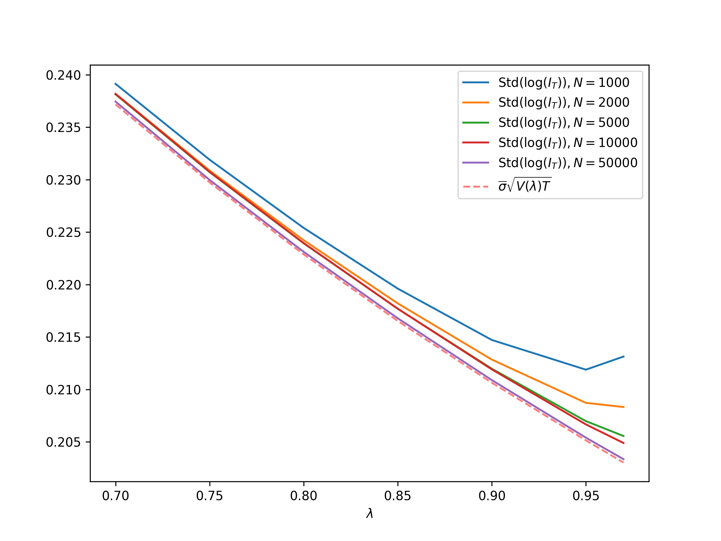
The rest of this paper is organised as follows. Section 2 is devoted to the proof of the main results, i.e. Theorem 1.5 and Proposition 1.7. Section 3 is devoted to the study of properties of the functions U(λ)U(\lambda) and V(λ)V(\lambda), and the derivation of the upper and lower bounds in (1.13) and (1.14). Limits of the volatility of ITI_{T} when (Δt,λ)(\Delta t,\lambda) approaches (0,1)(0,1) in different ways are discussed in Section 4, which provide quantification of the fact that, to achieve a preset volatility targeting quality, a smaller value of Δt\Delta t is needed when λ\lambda is closer to 11. In Section 5, we present some numerical test results confirming the conclusions of Theorem 1.5 and the results in Section 4.

2 Proof of the main results

This section consists of four subsections. In Section 2.1, we establish two limit theorems, Theorem 2.1, a strong law of large numbers, and Theorem 2.3, a central limit theorem. In Section 2.2, we show that the convergence of ITI_{T} can be reduced to a simpler process having a form for which the Theorem 2.1 and Theorem 2.3 can be easily applied (see Proposition 2.5 below). In Section 2.3, as an application of Theorem 2.1, Theorem 2.3, and Proposition 2.5, we establish Theorem 1.5 under the additional assumption that r(t)r(t), ρ(t)\rho(t), and σ(t)\sigma(t) are constants. In the last subsection, we prove the general case of Theorem 1.5 using the constant coefficient case and a continuity argument.

Throughout this section, we will adopt the convention that the notation cα1,,αkc_{\alpha_{1},\dots,\alpha_{k}} denotes a constant depending only on α1,,αk\alpha_{1},\dots,\alpha_{k}, and its value may vary at different appearances.

2.1 Two limit theorems

The proof of the constant coefficient case of Theorem 1.5 relies on Theorem 2.1 and Theorem 2.3 below, which are a law of large numbers and a central limit theorem for sequence of dependent random variables.

Theorem 2.1.

Let {λn}n0\{\lambda_{n}\}_{n\geq 0} be a sequence of non-negative numbers such that n=0λn=1\sum_{n=0}^{\infty}\lambda_{n}=1 and supn0γnλn<\sup_{n\geq 0}\gamma^{-n}\lambda_{n}<\infty for some constant γ(0,1)\gamma\in(0,1). Let {ξn}n1\{\xi_{n}\}_{n\geq 1} be a sequence of i.i.d. non-negative random variables, ω0>0\omega_{0}>0 be a constant, and

ωn=(1k=1nλnk)ω0+k=1nλnkξk,n1.\omega_{n}=\Big(1-\sum_{k=1}^{n}\lambda_{n-k}\Big)\omega_{0}+\sum_{k=1}^{n}\lambda_{n-k}\xi_{k},\quad n\geq 1. (2.1)

Suppose that the Laplace transform of ξ1\xi_{1}

ϕ(t)=𝔼(etξ1),t0,\phi(t)=\mathbb{E}(e^{-t\xi_{1}}),\quad t\geq 0, (2.2)

satisfies the property

1tαϕ(t)cϕ(1+t)β,1-t^{\alpha}\leq\phi(t)\leq c_{\phi}(1+t)^{-\beta}, (2.3)

for some constants 0<α1,β00<\alpha\leq 1,\beta\geq 0, and cϕ>0c_{\phi}>0. Let F(s)F(s) be a function on (0,)(0,\infty) satisfying the following properties:

  1. (P.1)

    0F(s)<0\leq F(s)<\infty on (0,)(0,\infty).

  2. (P.2)

    F(s) has non-negative inverse Laplace transform f0f\geq 0 with at most polynomial growth at infinity, that is

    F(s)=(f)(s)=0estf(t)𝑑t,s>0,F(s)=\mathcal{L}(f)(s)=\int_{0}^{\infty}e^{-st}f(t)dt,\quad s>0, (2.4)

    and

    f(t)cf(1+t)m,t1,f(t)\leq c_{f}(1+t)^{m},\quad t\geq 1, (2.5)

    for some constants cf>0c_{f}>0 and m0m\geq 0.

Then

limN1Nk=0N1F(ωk)=0f(t)k=0ϕ(λkt)dt<a.s.\lim_{N\to\infty}\frac{1}{N}\sum_{k=0}^{N-1}F(\omega_{k})=\int_{0}^{\infty}f(t)\prod_{k=0}^{\infty}\phi(\lambda_{k}t)dt<\infty\quad\text{a.s.} (2.6)
Remark 2.2.

(i) Below are some examples of the function F(s)F(s) satisfying the property (P.2).

  • F(s)=spF(s)=s^{-p} for any p>0p>0.

  • F(s)=ebs(s+a)nF(s)=e^{-bs}(s+a)^{-n} for any a,b>0a,b>0 and integer n1n\geq 1.

  • F(s)=s1(1ebs)F(s)=s^{-1}(1-e^{-bs}) for any b>0b>0.

  • If F(s)F(s) and G(s)G(s) satisfy the property (P.2), then F(s)+G(s)F(s)+G(s) and F(s)G(s)F(s)G(s) also satisfy the property (P.2).

(ii) An example of the sequence {λn}n0\{\lambda_{n}\}_{n\geq 0} is λn=(1λ)λn\lambda_{n}=(1-\lambda)\lambda^{n}, for which ωn=λnω0+k=1nλnkξk\omega_{n}=\lambda^{n}\omega_{0}+\sum_{k=1}^{n}\lambda^{n-k}\xi_{k}. Another example of {λn}n0\{\lambda_{n}\}_{n\geq 0} is λn=L1\lambda_{n}=L^{-1} when 0nL10\leq n\leq L-1, and λn=0\lambda_{n}=0 when nLn\geq L, for which ωn=1Lk=0L1ξnk\omega_{n}=\frac{1}{L}\sum_{k=0}^{L-1}\xi_{n-k}, nLn\geq L. For this case, the corresponding multiplier functions in (1.10) are given by U(L)=(L/2)1/2Γ[(L1)/2]/Γ(L/2)U(L)=(L/2)^{1/2}\Gamma[(L-1)/2]/\Gamma(L/2) and V(L)=L/(L2)V(L)=L/(L-2), with Γ(z)\Gamma(z) being the Gamma function.

Proof of Theorem 2.1.

We will prove the theorem in 3 steps.

Step 1. We first show that

limn𝔼(F(ωn))=0f(t)k=0ϕ(λkt)dt<,\lim_{n\to\infty}\mathbb{E}(F(\omega_{n}))=\int_{0}^{\infty}f(t)\prod_{k=0}^{\infty}\phi(\lambda_{k}t)dt<\infty, (2.7)

and

limn𝔼[F(ωn)2]=0(ff)(t)k=0ϕ(λkt)dt<,\lim_{n\to\infty}\mathbb{E}\big[F(\omega_{n})^{2}\big]=\int_{0}^{\infty}(f\ast f)(t)\prod_{k=0}^{\infty}\phi(\lambda_{k}t)dt<\infty, (2.8)

Let rn=k=nλkr_{n}=\sum_{k=n}^{\infty}\lambda_{k}. By (2.4) and Fubini’s theorem,

𝔼(F(ωn))\displaystyle\mathbb{E}(F(\omega_{n})) =𝔼(0f(t)eωnt𝑑t)=0f(t)𝔼(eωnt)𝑑t\displaystyle=\mathbb{E}\Big(\int_{0}^{\infty}f(t)e^{-\omega_{n}t}dt\Big)=\int_{0}^{\infty}f(t)\mathbb{E}\big(e^{-\omega_{n}t}\big)dt (2.9)
=0f(t)erntω0k=1n𝔼(eλnktξk)dt=0f(t)erntω0k=0n1ϕ(λnkt)dt.\displaystyle=\int_{0}^{\infty}f(t)e^{-r_{n}t\omega_{0}}\prod_{k=1}^{n}\mathbb{E}(e^{-\lambda_{n-k}t\xi_{k}})dt=\int_{0}^{\infty}f(t)e^{-r_{n}t\omega_{0}}\prod_{k=0}^{n-1}\phi(\lambda_{n-k}t)dt.

By (2.3) and (2.5), for sufficiently large KK\in\mathbb{N}, we have 1f(t)k=0K1ϕ(λkt)<\int_{1}^{\infty}f(t)\prod_{k=0}^{K-1}\phi(\lambda_{k}t)<\infty. Moreover, since F(s)<F(s)<\infty, we have

01f(t)k=0K1ϕ(λkt)dte01etf(t)𝑑teF(1)<.\int_{0}^{1}f(t)\prod_{k=0}^{K-1}\phi(\lambda_{k}t)dt\leq e\int_{0}^{1}e^{-t}f(t)dt\leq eF(1)<\infty.

Therefore,

0f(t)k=0K1ϕ(λkt)dt<,\int_{0}^{\infty}f(t)\prod_{k=0}^{K-1}\phi(\lambda_{k}t)dt<\infty,

which, together with ϕ(λkt)1\phi(\lambda_{k}t)\leq 1 and the dominated convergence theorem, implies (2.7).

For (2.8), since F2F^{2} also satisfies the property (P.2), by an argument similar to the above, we obtain that

𝔼[F(ωn)2]=0(ff)(t)erntω0k=0n1ϕ(λnkt)dt.\mathbb{E}\big[F(\omega_{n})^{2}\big]=\int_{0}^{\infty}(f\ast f)(t)e^{-r_{n}t\omega_{0}}\prod_{k=0}^{n-1}\phi(\lambda_{n-k}t)dt. (2.10)

Clearly, fff\ast f has at most polynomial growth at infinity. This, together with (2.3) and (2.10), implies (2.8).

Step 2. We next show that

Cov(F(ωn),F(ωn+k))cγ,f,ϕγαk,\text{Cov}(F(\omega_{n}),F(\omega_{n+k}))\leq c_{\gamma,f,\phi}\gamma^{\alpha k}, (2.11)

for all n,kn,k.

Since f0f\geq 0, we see that F(s)F(s) is decreasing in ss. Therefore,

𝔼[F(ωn)F(ωn+k)]\displaystyle\mathbb{E}\big[F(\omega_{n})F(\omega_{n+k})\big] =𝔼[F(ωn)F(rn+kω0+j=1n+kλn+kjξj)]𝔼[F(ωn)F(j=1kλkjξn+j)]\displaystyle=\mathbb{E}\Big[F(\omega_{n})F\Big(r_{n+k}\omega_{0}+\sum_{j=1}^{n+k}\lambda_{n+k-j}\xi_{j}\Big)\Big]\leq\mathbb{E}\Big[F(\omega_{n})F\Big(\sum_{j=1}^{k}\lambda_{k-j}\xi_{n+j}\Big)\Big]
=𝔼[F(ωn)]𝔼[F(j=1kλkjξn+j)]=𝔼[F(ωn)]𝔼[F(j=1kλkjξj)].\displaystyle=\mathbb{E}\big[F(\omega_{n})\big]\mathbb{E}\Big[F\Big(\sum_{j=1}^{k}\lambda_{k-j}\xi_{n+j}\Big)\Big]=\mathbb{E}\big[F(\omega_{n})\big]\mathbb{E}\Big[F\Big(\sum_{j=1}^{k}\lambda_{k-j}\xi_{j}\Big)\Big].

Applying (2.9) to the case ω0=0\omega_{0}=0 gives that

𝔼[F(ωn)F(ωn+k)]𝔼[F(ωn)]Jk,\mathbb{E}\big[F(\omega_{n})F(\omega_{n+k})\big]\leq\mathbb{E}\big[F(\omega_{n})\big]J_{k},

where

Jk=𝔼[F(j=1kλkjξj)]=0f(t)j=0k1ϕ(λkt)dt.J_{k}=\mathbb{E}\Big[F\Big(\sum_{j=1}^{k}\lambda_{k-j}\xi_{j}\Big)\Big]=\int_{0}^{\infty}f(t)\prod_{j=0}^{k-1}\phi(\lambda_{k}t)dt.

Hence,

Cov(F(ωn),F(ωn+k))\displaystyle\text{Cov}(F(\omega_{n}),F(\omega_{n+k})) =𝔼[F(ωn)F(ωn+k)]𝔼[F(ωn)]𝔼[F(ωn+k)]\displaystyle=\mathbb{E}\big[F(\omega_{n})F(\omega_{n+k})\big]-\mathbb{E}\big[F(\omega_{n})\big]\mathbb{E}\big[F(\omega_{n+k})\big] (2.12)
𝔼[F(ωn)](JkJn+k)+𝔼[F(ωn)](Jn+k𝔼[F(ωn+k)]).\displaystyle\leq\mathbb{E}\big[F(\omega_{n})\big](J_{k}-J_{n+k})+\mathbb{E}\big[F(\omega_{n})\big]\big(J_{n+k}-\mathbb{E}\big[F(\omega_{n+k})\big]\big).

For the first term in the last inequality of (2.12), we have

JkJn+k\displaystyle J_{k}-J_{n+k} =0f(t)(j=0k1ϕ(λjt))(1j=0n1ϕ(λk+jt))𝑑t0f(t)(1j=0n1ϕ(λk+jt))𝑑t.\displaystyle=\int_{0}^{\infty}f(t)\Big(\prod_{j=0}^{k-1}\phi(\lambda_{j}t)\Big)\Big(1-\prod_{j=0}^{n-1}\phi(\lambda_{k+j}t)\Big)dt\leq\int_{0}^{\infty}f(t)\Big(1-\prod_{j=0}^{n-1}\phi(\lambda_{k+j}t)\Big)dt.

Denote A=supn0γnλn<A=\sup_{n\geq 0}\gamma^{-n}\lambda_{n}<\infty. By (2.3) and λnAγn\lambda_{n}\leq A\gamma^{n},

1j=0n1ϕ(λk+jt)\displaystyle 1-\prod_{j=0}^{n-1}\phi(\lambda_{k+j}t) =l=0n1(j=l+1n1ϕ(λk+jt)j=ln1ϕ(λk+jt))\displaystyle=\sum_{l=0}^{n-1}\Big(\prod_{j=l+1}^{n-1}\phi(\lambda_{k+j}t)-\prod_{j=l}^{n-1}\phi(\lambda_{k+j}t)\Big)
=l=0n1[1ϕ(λk+lt)]j=l+1n1ϕ(λk+j)l=0n1[1ϕ(λk+lt)]Aαγαktα1γα,\displaystyle=\sum_{l=0}^{n-1}[1-\phi(\lambda_{k+l}t)]\prod_{j=l+1}^{n-1}\phi(\lambda_{k+j})\leq\sum_{l=0}^{n-1}[1-\phi(\lambda_{k+l}t)]\leq\frac{A^{\alpha}\gamma^{\alpha k}t^{\alpha}}{1-\gamma^{\alpha}},

where we use the convention that j=l+1n1ϕ(λk+jt)=1\prod_{j=l+1}^{n-1}\phi(\lambda_{k+j}t)=1 when l+1>n1l+1>n-1. Let KK be an integer such that K>(m+2)/βK>(m+2)/\beta. By (2.3) and (2.5), 0tαf(t)j=0K1ϕ(λjt)dt<\int_{0}^{\infty}t^{\alpha}f(t)\prod_{j=0}^{K-1}\phi(\lambda_{j}t)dt<\infty. Therefore, for any k>Kk>K,

JkJn+k\displaystyle J_{k}-J_{n+k} Aαγαk1γα0tαf(t)j=0k1ϕ(λjt)dt\displaystyle\leq\frac{A^{\alpha}\gamma^{\alpha k}}{1-\gamma^{\alpha}}\int_{0}^{\infty}t^{\alpha}f(t)\prod_{j=0}^{k-1}\phi(\lambda_{j}t)dt
Aαγαk1γα0tαf(t)j=0K1ϕ(λjt)dt=cγ,f,ϕγαk.\displaystyle\leq\frac{A^{\alpha}\gamma^{\alpha k}}{1-\gamma^{\alpha}}\int_{0}^{\infty}t^{\alpha}f(t)\prod_{j=0}^{K-1}\phi(\lambda_{j}t)dt=c_{\gamma,f,\phi}\gamma^{\alpha k}.

This, together with (2.7), implies that

𝔼[F(ωn)](JkJn+k)cγ,f,ϕγαk.\mathbb{E}\big[F(\omega_{n})\big](J_{k}-J_{n+k})\leq c_{\gamma,f,\phi}\gamma^{\alpha k}. (2.13)

For the second term in the last inequality of (2.12), let KK be same integer as above. By (2.3) and (2.5), 0tf(t)j=0K1ϕ(λjt)dt<\int_{0}^{\infty}tf(t)\prod_{j=0}^{K-1}\phi(\lambda_{j}t)dt<\infty. Therefore, for kKk\geq K,

Jn+k𝔼[F(ωn+k)]\displaystyle J_{n+k}-\mathbb{E}\big[F(\omega_{n+k})\big] 0f(t)(1ern+ktω0)j=0n+k1ϕ(λjt)dt\displaystyle\leq\int_{0}^{\infty}f(t)\big(1-e^{-r_{n+k}t\omega_{0}}\big)\prod_{j=0}^{n+k-1}\phi(\lambda_{j}t)dt
rn+kω00tf(t)j=0n+k1ϕ(λjt)dtrn+kω00tf(t)j=0K1ϕ(λjt)dt=cf,ϕω0rn+k.\displaystyle\leq r_{n+k}\omega_{0}\int_{0}^{\infty}tf(t)\prod_{j=0}^{n+k-1}\phi(\lambda_{j}t)dt\leq r_{n+k}\omega_{0}\int_{0}^{\infty}tf(t)\prod_{j=0}^{K-1}\phi(\lambda_{j}t)dt=c_{f,\phi}\omega_{0}r_{n+k}.

By rn+kAj=n+kγjcγγn+kr_{n+k}\leq A\sum_{j=n+k}^{\infty}\gamma^{j}\leq c_{\gamma}\gamma^{n+k} and (2.7), we obtain that

𝔼[F(ωn)](Jn+k𝔼[F(ωn+k)])cγ,f,ϕγn+k.\mathbb{E}\big[F(\omega_{n})\big]\big(J_{n+k}-\mathbb{E}\big[F(\omega_{n+k})\big]\big)\leq c_{\gamma,f,\phi}\gamma^{n+k}. (2.14)

Combining (2.13) and (2.14) gives (2.11).

Step 3. We now prove the a.s. convergence (2.6).

By (2.8), we have L=supnVar(F(ωn))<L=\sup_{n}\text{Var}(F(\omega_{n}))<\infty. Denote ψn=1nk=0n1F(ωk)\psi_{n}=\frac{1}{n}\sum_{k=0}^{n-1}F(\omega_{k}). By (2.11),

Var(ψn)\displaystyle\text{Var}(\psi_{n}) =n2k=0n1Var(F(ωk))+2n21k<lnCov(F(ωk),F(ωl))\displaystyle=n^{-2}\sum_{k=0}^{n-1}\text{Var}(F(\omega_{k}))+2n^{-2}\sum_{1\leq k<l\leq n}\text{Cov}(F(\omega_{k}),F(\omega_{l})) (2.15)
n1L+2cγ,f,ϕn2k=1nl=k+1nγα(lk)n1(L+2cγ,f,ϕγα1γα).\displaystyle\leq n^{-1}L+2c_{\gamma,f,\phi}n^{-2}\sum_{k=1}^{n}\sum_{l=k+1}^{n}\gamma^{\alpha(l-k)}\leq n^{-1}\Big(L+2c_{\gamma,f,\phi}\frac{\gamma^{\alpha}}{1-\gamma^{\alpha}}\Big).

To derive the a.s. convergence of limnψn\lim_{n\to\infty}\psi_{n} from the variance estimate (2.15), we use an argument similar to that in [1]. For any θ>1\theta>1, let θn=θn\theta_{n}=\lfloor\theta^{n}\rfloor be the integer part of θn\theta^{n}. Then θnθn/2\theta_{n}\geq\theta^{n}/2. Hence, for any ϵ>0\epsilon>0,

n=1(|ψθn𝔼(ψθn)|>ϵ)ϵ2n=1Var(ψθn)\displaystyle\sum_{n=1}^{\infty}\mathbb{P}\big(|\psi_{\theta_{n}}-\mathbb{E}(\psi_{\theta_{n}})|>\epsilon\big)\leq\epsilon^{-2}\sum_{n=1}^{\infty}\text{Var}(\psi_{\theta_{n}})
ϵ1(L2+cγ,f,ϕγα1γα)n=1θn1ϵ2(L2+cγ,f,ϕγα1γα)n=1θn<.\displaystyle\hskip 30.00005pt\leq\epsilon^{-1}\Big(\frac{L}{2}+c_{\gamma,f,\phi}\frac{\gamma^{\alpha}}{1-\gamma^{\alpha}}\Big)\sum_{n=1}^{\infty}\theta_{n}^{-1}\leq\epsilon^{-2}\Big(\frac{L}{2}+c_{\gamma,f,\phi}\frac{\gamma^{\alpha}}{1-\gamma^{\alpha}}\Big)\sum_{n=1}^{\infty}\theta^{-n}<\infty.

By the Borel–Cantelli lemma, limn[ψθn𝔼(ψθn)]=0\lim_{n\to\infty}\big[\psi_{\theta_{n}}-\mathbb{E}(\psi_{\theta_{n}})\big]=0 a.s. By (2.7), we see that

limnψθn=J=0f(t)k=0ϕ(λkt)dta.s.\lim_{n\to\infty}\psi_{\theta_{n}}=J_{\infty}=\int_{0}^{\infty}f(t)\prod_{k=0}^{\infty}\phi(\lambda_{k}t)dt\quad\text{a.s.}

For any n>0n>0, let k(n)k(n) be such that θk(n)<nθk(n)+1\theta_{k(n)}<n\leq\theta_{k(n)+1}. Then θk(n)+1/θk(n)θ\theta_{k(n)+1}/\theta_{k(n)}\leq\theta. Clearly nψnn\psi_{n} is increasing in nn. Therefore,

θk(n)θk(n)+1ψθk(n)nθk(n)+1ψnψnnθk(n)ψnθk(n)+1θk(n)ψθk(n)+1.\frac{\theta_{k(n)}}{\theta_{k(n)+1}}\psi_{\theta_{k(n)}}\leq\frac{n}{\theta_{k(n)+1}}\psi_{n}\leq\psi_{n}\leq\frac{n}{\theta_{k(n)}}\psi_{n}\leq\frac{\theta_{k(n)+1}}{\theta_{k(n)}}\psi_{\theta_{k(n)+1}}.

Setting nn\to\infty gives that

θ1Jlim infnψnlim supnψnθJa.s.\theta^{-1}J_{\infty}\leq\liminf_{n\to\infty}\psi_{n}\leq\limsup_{n\to\infty}\psi_{n}\leq\theta J_{\infty}\quad\text{a.s.}

for any θ>1\theta>1, which implies that

limnψn=J=0f(t)k=0ϕ(λkt)dta.s.\lim_{n\to\infty}\psi_{n}=J_{\infty}=\int_{0}^{\infty}f(t)\prod_{k=0}^{\infty}\phi(\lambda_{k}t)dt\quad\text{a.s.}

This completes the proof. ∎

Theorem 2.3.

Let {λn}n0\{\lambda_{n}\}_{n\geq 0} be a sequence of non-negative numbers satisfying the conditions n=0λn=1\sum_{n=0}^{\infty}\lambda_{n}=1 and supn0γnλn<\sup_{n\geq 0}\gamma^{-n}\lambda_{n}<\infty for some γ(0,1)\gamma\in(0,1). Let {ξn}n1\{\xi_{n}\}_{n\geq 1} be a sequence of i.i.d. random variables of which the Laplace transform ϕ(t)=𝔼(etξ1)\phi(t)=\mathbb{E}(e^{-t\xi_{1}}) satisfies the property (2.3), and F(s)F(s) be a completely monotone function satisfying the properties (P.1) and (P.2) in Theorem 2.1. Let ω0>0\omega_{0}>0 be a constant and {ωn}n1\{\omega_{n}\}_{n\geq 1} be the sequence defined by (2.1). Suppose that {ηn}n1\{\eta_{n}\}_{n\geq 1} is a sequence of random variables such that ηn+1\eta_{n+1} is independent of {(ξk,ηk):1kn}\{(\xi_{k},\eta_{k}):1\leq k\leq n\}, and

𝔼(ηn)=0,\mathbb{E}(\eta_{n})=0,

and

limn𝔼(ηn2)=1.\lim_{n\to\infty}\mathbb{E}(\eta_{n}^{2})=1.

Suppose, in addition, that supn1𝔼(|ηn|p)<\sup_{n\geq 1}\mathbb{E}(|\eta_{n}|^{p})<\infty for some p>2p>2. Then

1Nk=1NF(ωk1)ηk𝒩(0,0(ff)(t)k=0ϕ(λkt)dt),\frac{1}{\sqrt{N}}\sum_{k=1}^{N}F(\omega_{k-1})\eta_{k}\to\mathcal{N}\Big(0,\int_{0}^{\infty}(f\ast f)(t)\prod_{k=0}^{\infty}\phi(\lambda_{k}t)dt\Big), (2.16)

in distribution as NN\to\infty, where 𝒩(μ,σ2)\mathcal{N}(\mu,\sigma^{2}) is the normal distribution with mean μ\mu and variance σ2\sigma^{2}, f=1(F)f=\mathcal{L}^{-1}(F) is the inverse Laplace transform of FF, and the convolution fff\ast f is defined by extending f|(,0)=0f|_{(-\infty,0)}=0.

Proof.

Let Mn=k=1nF(ωk1)ηk,M_{n}=\sum_{k=1}^{n}F(\omega_{k-1})\eta_{k}, M0=0M_{0}=0. Clearly, {Mn}n1\{M_{n}\}_{n\geq 1} is a martingale in view of 𝔼(ηn)=0\mathbb{E}(\eta_{n})=0. Let n=σ(ξk,ηk:1kn)\mathcal{F}_{n}=\sigma(\xi_{k},\eta_{k}:1\leq k\leq n) be the filtration generated by {(ξn,ηn)}n1\{(\xi_{n},\eta_{n})\}_{n\geq 1}, and define

sn\displaystyle s_{n} =k=1nVar(MkMk1)=k=1nVar(F(ωk1)ηk),\displaystyle=\sum_{k=1}^{n}\text{Var}(M_{k}-M_{k-1})=\sum_{k=1}^{n}\text{Var}\big(F(\omega_{k-1})\eta_{k}\big),
vn\displaystyle v_{n} =k=1nVar(MkMk1|k1)=k=1nVar(F(ωk1)ηk|k1).\displaystyle=\sum_{k=1}^{n}\text{Var}(M_{k}-M_{k-1}|\mathcal{F}_{k-1})=\sum_{k=1}^{n}\text{Var}\big(F(\omega_{k-1})\eta_{k}|\mathcal{F}_{k-1}\big).

By independence of ηk\eta_{k} and k1\mathcal{F}_{k-1}, we have sn=k=1n𝔼(F(ωk1)2)s_{n}=\sum_{k=1}^{n}\mathbb{E}\big(F(\omega_{k-1})^{2}\big) and vn=k=1nF(ωk1)2v_{n}=\sum_{k=1}^{n}F(\omega_{k-1})^{2}. We will show that the Lindeberg condition

limn1nk=1n𝔼[F(ωk1)2ηk2χ{|F(ωk1)ηk|>ϵn}]=0,\lim_{n\to\infty}\frac{1}{n}\sum_{k=1}^{n}\mathbb{E}\big[F(\omega_{k-1})^{2}\eta_{k}^{2}\chi_{\{|F(\omega_{k-1})\eta_{k}|>\epsilon\sqrt{n}\}}\big]=0, (2.17)

holds for any ϵ>0\epsilon>0, and that

limnsnvn=1a.s.\lim_{n\to\infty}\frac{s_{n}}{v_{n}}=1\quad\text{a.s.} (2.18)

Once (2.17) and (2.18) are proved, by the martingale central limit theorem (see for example [3, page 9–10]), we may deduce that

1sNk=1NF(ωk1)ηk𝒩(0,1),\frac{1}{\sqrt{s_{N}}}\sum_{k=1}^{N}F(\omega_{k-1})\eta_{k}\to\mathcal{N}(0,1), (2.19)

in distribution. Moreover, by (2.8), we have

limnsnn=limn𝔼(F(ωn)2)=0(ff)(t)k=0ϕ(λkt)dta.s.\lim_{n\to\infty}\frac{s_{n}}{n}=\lim_{n\to\infty}\mathbb{E}\big(F(\omega_{n})^{2}\big)=\int_{0}^{\infty}(f\ast f)(t)\prod_{k=0}^{\infty}\phi(\lambda_{k}t)dt\quad\text{a.s.} (2.20)

Combining (2.19) and (2.20) proves the desired convergence (2.16).

To prove that the Lindeberg condition (2.17) holds, for any integer m1m\geq 1, note that by the properties of completely monotone functions (see for example [SSV12, Chapter 1]), FpF^{p} satisfies the properties (P.1) and (P.2). Applying (2.7) to FpF^{p} gives that supn1𝔼(F(ωk1)p)cp,γ,f,ϕ<\sup_{n\geq 1}\mathbb{E}(F(\omega_{k-1})^{p})\leq c_{p,\gamma,f,\phi}<\infty. Let A=supn1𝔼(|ηn|p)A=\sup_{n\geq 1}\mathbb{E}(|\eta_{n}|^{p}). Then

𝔼[F(ωk1)2ηk2χ{|F(ωk1)ηk|>ϵn}]\displaystyle\mathbb{E}\big[F(\omega_{k-1})^{2}\eta_{k}^{2}\chi_{\{|F(\omega_{k-1})\eta_{k}|>\epsilon\sqrt{n}\}}\big] 1ϵp2np/21𝔼[F(ωk1)p|ηk|p]\displaystyle\leq\frac{1}{\epsilon^{p-2}n^{p/2-1}}\mathbb{E}\big[F(\omega_{k-1})^{p}|\eta_{k}|^{p}\big]
=1ϵp2np/21𝔼[F(ωk1)p]𝔼[|ηk|p]cp,γ,f,ϕAϵp2np/21.\displaystyle=\frac{1}{\epsilon^{p-2}n^{p/2-1}}\mathbb{E}\big[F(\omega_{k-1})^{p}\big]\mathbb{E}\big[|\eta_{k}|^{p}\big]\leq\frac{c_{p,\gamma,f,\phi}A}{\epsilon^{p-2}n^{p/2-1}}.

Therefore,

1nk=1n𝔼[F(ωk1)2ηk2χ{|F(ωk1)ηk|>ϵn}]cp,γ,f,ϕAϵp2np/210,\frac{1}{n}\sum_{k=1}^{n}\mathbb{E}\big[F(\omega_{k-1})^{2}\eta_{k}^{2}\chi_{\{|F(\omega_{k-1})\eta_{k}|>\epsilon\sqrt{n}\}}\big]\leq\frac{c_{p,\gamma,f,\phi}A}{\epsilon^{p-2}n^{p/2-1}}\to 0,

as nn\to\infty.

It remains to prove (2.18). Note that F2F^{2} also satisfies the properties (P.1) and (P.2). By Theorem 2.1, we obtain that

limnvnn=0(ff)(t)k=0ϕ(λkt)dta.s.,\lim_{n\to\infty}\frac{v_{n}}{n}=\int_{0}^{\infty}(f\ast f)(t)\prod_{k=0}^{\infty}\phi(\lambda_{k}t)dt\quad\text{a.s.}, (2.21)

which, together with (2.20) implies (2.18). This completes the proof of Theorem 2.3. ∎

2.2 Reduction to an equivalent convergence

For this subsection and the rest of this paper, we will denote processes such as ItI_{t} and vnv_{n} by It(N)I_{t}^{(N)} and vn(N)v_{n}^{(N)} when it is necessary to indicate their dependence on Δt\Delta t. Then

logIT(N)I0\displaystyle\log\frac{I_{T}^{(N)}}{I_{0}} =0Tr(t)𝑑t+k=1Nσ¯vk1(N)tk1tk[ρ(t)r(t)]𝑑t\displaystyle=\int_{0}^{T}r(t)dt+\sum_{k=1}^{N}\dfrac{\bar{\sigma}}{\sqrt{v_{k-1}^{(N)}}}\int_{t_{k-1}}^{t_{k}}[\rho(t)-r(t)]dt (2.22)
12k=1Nσ¯2vk1(N)tk1tkσ(t)2𝑑t+k=1Nσ¯vk1(N)tk1tkσ(t)𝑑Wt,\displaystyle-\frac{1}{2}\sum_{k=1}^{N}\dfrac{\bar{\sigma}^{2}}{v_{k-1}^{(N)}}\int_{t_{k-1}}^{t_{k}}\sigma(t)^{2}dt+\sum_{k=1}^{N}\dfrac{\bar{\sigma}}{\sqrt{v_{k-1}^{(N)}}}\int_{t_{k-1}}^{t_{k}}\sigma(t)dW_{t},

We shall show that the convergence of IT(N)I_{T}^{(N)} in distribution is equivalent to that of a simpler random variable XT(N)X_{T}^{(N)} defined by

dXt(N)Xt(N)\displaystyle\frac{dX_{t}^{(N)}}{X_{t}^{(N)}} =(1σ¯utn1(N))r(t)dt+σ¯utn1(N)dStSt,t[tn1,tn),\displaystyle=\Big(1-\frac{\bar{\sigma}}{\sqrt{u_{t_{n-1}}^{(N)}}}\Big)r(t)dt+\frac{\bar{\sigma}}{\sqrt{u_{t_{n-1}}^{(N)}}}\frac{dS_{t}}{S_{t}},\quad t\in[t_{n-1},t_{n}), (2.23)
X0(N)\displaystyle X_{0}^{(N)} =I0,\displaystyle=I_{0},

where

un(N)\displaystyle u_{n}^{(N)} =λun1(N)+1λΔt(tk1tkσ(t)𝑑Wt)2,u0(N)=v0,\displaystyle=\lambda u_{n-1}^{(N)}+\frac{1-\lambda}{\Delta t}\Big(\int_{t_{k-1}}^{t_{k}}\sigma(t)dW_{t}\Big)^{2},\quad u_{0}^{(N)}=v_{0},

or equivalently,

logXT(N)I0\displaystyle\log\frac{X_{T}^{(N)}}{I_{0}} =0Tr(t)𝑑t+k=1Nσ¯uk1(N)tk1tk[ρ(t)r(t)]𝑑t\displaystyle=\int_{0}^{T}r(t)dt+\sum_{k=1}^{N}\dfrac{\bar{\sigma}}{\sqrt{u_{k-1}^{(N)}}}\int_{t_{k-1}}^{t_{k}}[\rho(t)-r(t)]dt (2.24)
12k=1Nσ¯2uk1(N)tk1tkσ(t)2𝑑t+k=1Nσ¯uk1(N)tk1tkσ(t)𝑑Wt\displaystyle-\frac{1}{2}\sum_{k=1}^{N}\dfrac{\bar{\sigma}^{2}}{u_{k-1}^{(N)}}\int_{t_{k-1}}^{t_{k}}\sigma(t)^{2}dt+\sum_{k=1}^{N}\dfrac{\bar{\sigma}}{\sqrt{u_{k-1}^{(N)}}}\int_{t_{k-1}}^{t_{k}}\sigma(t)dW_{t}

and

un(N)=λnv0+1λΔtk=1nλnk(tk1tkσ(t)𝑑Wt)2.u_{n}^{(N)}=\lambda^{n}v_{0}+\frac{1-\lambda}{\Delta t}\sum_{k=1}^{n}\lambda^{n-k}\Big(\int_{t_{k-1}}^{t_{k}}\sigma(t)dW_{t}\Big)^{2}. (2.25)

We start with the following lemma.

Lemma 2.4.

For any h(x)=xαh(x)=x^{-\alpha}, α>0\alpha>0, we have

supN1supn<N𝔼[h(un(N))]cα,λ,v0,σ<,\sup_{N\geq 1}\sup_{n<N}\mathbb{E}\big[h(u_{n}^{(N)})\big]\leq c_{\alpha,\lambda,v_{0},\sigma_{\ast}}<\infty, (2.26)
supN1supn<N𝔼[h(vn(N))]cα,λ,v0,σ<,\sup_{N\geq 1}\sup_{n<N}\mathbb{E}\big[h(v_{n}^{(N)})\big]\leq c_{\alpha,\lambda,v_{0},\sigma_{\ast}}<\infty, (2.27)

for some constant cα,λ,v0,σc_{\alpha,\lambda,v_{0},\sigma_{\ast}} depending only on α,λ,v0,σ\alpha,\lambda,v_{0},\sigma_{\ast}, and for any p1p\geq 1,

limNsupn<N𝔼[|h(un(N))h(vn(N))|p]=0.\lim_{N\to\infty}\sup_{n<N}\mathbb{E}\big[|h(u_{n}^{(N)})-h(v_{n}^{(N)})|^{p}\big]=0. (2.28)
Proof.

We first prove (2.26). Note that the inverse Laplace transform of h(x)h(x) is 1(h)(t)=tα1/Γ(α).\mathcal{L}^{-1}(h)(t)=t^{\alpha-1}/\Gamma(\alpha). Therefore, by Fubini’s theorem,

𝔼[h(un(N))]\displaystyle\mathbb{E}\big[h(u_{n}^{(N)})\big] =𝔼[1Γ(α)0tα1eun(N)t𝑑t]\displaystyle=\mathbb{E}\Big[\frac{1}{\Gamma(\alpha)}\int_{0}^{\infty}t^{\alpha-1}e^{-u_{n}^{(N)}t}dt\Big] (2.29)
=1Γ(α)0tα1𝔼(eun(N)t)𝑑t=1Γ(α)0tα1eλnv0tk=1n1𝔼(k)dt,\displaystyle=\frac{1}{\Gamma(\alpha)}\int_{0}^{\infty}t^{\alpha-1}\mathbb{E}\big(e^{-u_{n}^{(N)}t}\big)dt=\frac{1}{\Gamma(\alpha)}\int_{0}^{\infty}t^{\alpha-1}e^{-\lambda^{n}v_{0}t}\prod_{k=1}^{n-1}\mathbb{E}(\mathcal{E}_{k})dt,

where k=exp(1λΔttλnk(tk1tkσ(t)𝑑Wt)2)\mathcal{E}_{k}=\exp\Big(-\frac{1-\lambda}{\Delta t}t\lambda^{n-k}\Big(\int_{t_{k-1}}^{t_{k}}\sigma(t)dW_{t}\Big)^{2}\Big). Recall that for a standard normal distribution ZZ and any a,σ>0a,\sigma>0, μ\mu\in\mathbb{R}, we have

𝔼[ea(μ+σZ)2]=(1+2aσ2)1/2exp(aμ21+2aσ2).\mathbb{E}[e^{-a(\mu+\sigma Z)^{2}}]=(1+2a\sigma^{2})^{-1/2}\exp\Big(-\frac{a\mu^{2}}{1+2a\sigma^{2}}\Big). (2.30)

Since tk1tkσ(t)𝑑Wt\int_{t_{k-1}}^{t_{k}}\sigma(t)dW_{t} is a normal distribution with mean zero and variance tk1tkσ(t)2𝑑t\int_{t_{k-1}}^{t_{k}}\sigma(t)^{2}dt, by (2.30),

𝔼(k)=[1+21λΔttλnk(tk1tkσ(t)2𝑑t)]1/2[1+2t(1λ)λnkσ2]1/2.\mathbb{E}(\mathcal{E}_{k})=\Big[1+2\frac{1-\lambda}{\Delta t}t\lambda^{n-k}\Big(\int_{t_{k-1}}^{t_{k}}\sigma(t)^{2}dt\Big)\Big]^{-1/2}\leq[1+2t(1-\lambda)\lambda^{n-k}\sigma_{\ast}^{2}]^{-1/2}.

Therefore, by the above and (2.29),

𝔼[h(un(N))]1Γ(α)0tα1eλnv0tk=0n1[1+2t(1λ)λkσ2]1/2dt.\mathbb{E}\big[h(u_{n}^{(N)})\big]\leq\frac{1}{\Gamma(\alpha)}\int_{0}^{\infty}t^{\alpha-1}e^{-\lambda^{n}v_{0}t}\prod_{k=0}^{n-1}[1+2t(1-\lambda)\lambda^{k}\sigma_{\ast}^{2}]^{-1/2}dt. (2.31)

Let mm be an integer such that m>2αm>2\alpha. For nmn\geq m, by (2.31),

𝔼[h(un(N))]1Γ(α)0tα1k=0m1[1+2t(1λ)λkσ2]1/2dt.\begin{aligned} \mathbb{E}\big[h(u_{n}^{(N)})\big]&\leq\frac{1}{\Gamma(\alpha)}\int_{0}^{\infty}t^{\alpha-1}\prod_{k=0}^{m-1}[1+2t(1-\lambda)\lambda^{k}\sigma_{\ast}^{2}]^{-1/2}dt\end{aligned}. (2.32)

For n<mn<m, by (2.31) again,

𝔼[h(un(N))]1Γ(α)0tα1eλmv0t𝑑t.\mathbb{E}\big[h(u_{n}^{(N)})\big]\leq\frac{1}{\Gamma(\alpha)}\int_{0}^{\infty}t^{\alpha-1}e^{-\lambda^{m}v_{0}t}dt. (2.33)

The uniform L1L^{1} bound (2.26) follows from (2.32) and (2.33).

We next prove (2.27). Denote θk=tk1tk(ρ(t)σ(t)2/2)𝑑t\theta_{k}=\int_{t_{k-1}}^{t_{k}}(\rho(t)-\sigma(t)^{2}/2)dt, Yk=tk1tkσ(t)𝑑WtY_{k}=\int_{t_{k-1}}^{t_{k}}\sigma(t)dW_{t}, and Rk=(Δt)1/2(θk+Yk)R_{k}=(\Delta t)^{-1/2}(\theta_{k}+Y_{k}). Then

vn(N)=λnv0+1λΔtk=1nλnk[eΔtRk1]2.v_{n}^{(N)}=\lambda^{n}v_{0}+\frac{1-\lambda}{\Delta t}\sum_{k=1}^{n}\lambda^{n-k}\big[e^{\sqrt{\Delta t}R_{k}}-1\big]^{2}.

Note that

1Δt|eΔtx1|eΔt|x|χ{x1}+1eTTχ{x<1}.\frac{1}{\sqrt{\Delta t}}\big|e^{\sqrt{\Delta t}x}-1\big|\geq e^{-\sqrt{\Delta t}}|x|\chi_{\{x\geq-1\}}+\frac{1-e^{-\sqrt{T}}}{\sqrt{T}}\chi_{\{x<-1\}}. (2.34)

Indeed, for x0x\geq 0, we have |eΔtx1|/Δt|x||e^{\sqrt{\Delta t}x}-1|/\sqrt{\Delta t}\geq|x|. When 1x<0-1\leq x<0, we have |eΔtx1|/Δt=eΔtx(eΔtx1)/ΔteΔt|x||e^{\sqrt{\Delta t}x}-1|/\sqrt{\Delta t}=e^{-\sqrt{\Delta t}x}\big(e^{\sqrt{\Delta t}x}-1\big)/\sqrt{\Delta t}\geq e^{-\sqrt{\Delta t}}|x|. When x<1x<-1, we have |eΔtx1|/Δt(1eΔt)/Δt(1eT)/T|e^{\sqrt{\Delta t}x}-1|/\sqrt{\Delta t}\geq(1-e^{-\sqrt{\Delta t}})/\sqrt{\Delta t}\geq(1-e^{-\sqrt{T}})/\sqrt{T}. By (2.34),

𝔼[exp(t(1λ)λnk(eΔtRk1)2Δt)]\displaystyle\mathbb{E}\Big[\exp\Big(-t(1-\lambda)\lambda^{n-k}\frac{(e^{\sqrt{\Delta t}R_{k}}-1)^{2}}{\Delta t}\Big)\Big] 𝔼[et(1λ)λnkRk2+exp(t(1λ)λnk(1eΔt)2Δt)]\displaystyle\leq\mathbb{E}\Big[e^{-t(1-\lambda)\lambda^{n-k}R_{k}^{2}}+\exp\Big(-t(1-\lambda)\lambda^{n-k}\frac{(1-e^{-\sqrt{\Delta t}})^{2}}{\Delta t}\Big)\Big] (2.35)
𝔼[et(1λ)λnkRk2]+ecTt(1λ)λnk.\displaystyle\leq\mathbb{E}\big[e^{-t(1-\lambda)\lambda^{n-k}R_{k}^{2}}\big]+e^{-c_{T}t(1-\lambda)\lambda^{n-k}}.

Since RkR_{k} is a normal distribution with mean (Δt)1/2θk(\Delta t)^{-1/2}\theta_{k} and variance σk2=(Δt)1tk1tkσ(t)2𝑑t\sigma_{k}^{2}=(\Delta t)^{-1}\int_{t_{k-1}}^{t_{k}}\sigma(t)^{2}dt, by (2.30),

𝔼[et(1λ)λnkRk2]\displaystyle\mathbb{E}\big[e^{-t(1-\lambda)\lambda^{n-k}R_{k}^{2}}\big] =[1+2t(1λ)λnkσk2]1/2exp(t(1λ)λnkθk2(Δt)11+2t(1λ)λnkσk2).\displaystyle=[1+2t(1-\lambda)\lambda^{n-k}\sigma_{k}^{2}]^{-1/2}\exp\Big(-\frac{t(1-\lambda)\lambda^{n-k}\theta_{k}^{2}(\Delta t)^{-1}}{1+2t(1-\lambda)\lambda^{n-k}\sigma_{k}^{2}}\Big).

By σ(t)σ\sigma(t)\geq\sigma_{\ast}, we obtain that 𝔼[et(1λ)λnkRk2][1+2t(1λ)λnkσ2]1/2\mathbb{E}\big[e^{-t(1-\lambda)\lambda^{n-k}R_{k}^{2}}\big]\leq[1+2t(1-\lambda)\lambda^{n-k}\sigma_{\ast}^{2}]^{-1/2}, and therefore, by (2.35)

𝔼[exp(t(1λ)λnk(eΔtRk1)2Δt)]\displaystyle\mathbb{E}\Big[\exp\Big(-t(1-\lambda)\lambda^{n-k}\frac{(e^{\sqrt{\Delta t}R_{k}}-1)^{2}}{\Delta t}\Big)\Big] [1+2t(1λ)λnkσ2]1/2+ecTt(1λ)λnk\displaystyle\leq[1+2t(1-\lambda)\lambda^{n-k}\sigma_{\ast}^{2}]^{-1/2}+e^{-c_{T}t(1-\lambda)\lambda^{n-k}}
cσ,T[1+t(1λ)λnk]1/2.\displaystyle\leq c_{\sigma_{\ast},T}[1+t(1-\lambda)\lambda^{n-k}]^{-1/2}.

Moreover,

𝔼[h(vn(N))]\displaystyle\mathbb{E}\big[h(v_{n}^{(N)})\big] =1Γ(α)0tα1eλnv0tk=1n1𝔼[exp(t(1λ)λnk(eΔtRk1)2Δt)]dt\displaystyle=\frac{1}{\Gamma(\alpha)}\int_{0}^{\infty}t^{\alpha-1}e^{-\lambda^{n}v_{0}t}\prod_{k=1}^{n-1}\mathbb{E}\Big[\exp\Big(-t(1-\lambda)\lambda^{n-k}\frac{(e^{\sqrt{\Delta t}R_{k}}-1)^{2}}{\Delta t}\Big)\Big]dt
cσ,TΓ(α)0tα1eλnv0tk=1n1[1+t(1λ)λnk]1/2dt,\displaystyle\leq\frac{c_{\sigma_{\ast},T}}{\Gamma(\alpha)}\int_{0}^{\infty}t^{\alpha-1}e^{-\lambda^{n}v_{0}t}\prod_{k=1}^{n-1}[1+t(1-\lambda)\lambda^{n-k}]^{-1/2}dt,

which, similar to the proof of (2.26), implies the uniform L1L^{1}-bound (2.27).

We now prove the uniform convergence (2.28). It suffices to prove this for integer-valued pp. By Hölder’s inequality,

𝔼(|un(N)vn(N)|2p)\displaystyle\mathbb{E}\big(|u_{n}^{(N)}-v_{n}^{(N)}|^{2p}\big) 𝔼[(1λΔtk=1nλnk|(eθk+Yk1)2Yk2|)2p]\displaystyle\leq\mathbb{E}\Big[\Big(\frac{1-\lambda}{\Delta t}\sum_{k=1}^{n}\lambda^{n-k}\big|(e^{\theta_{k}+Y_{k}}-1)^{2}-Y_{k}^{2}\big|\Big)^{2p}\Big] (2.36)
𝔼(1λ(Δt)2pk=1nλnk|(eθk+Yk1)2Yk2|2p)\displaystyle\leq\mathbb{E}\Big(\frac{1-\lambda}{(\Delta t)^{2p}}\sum_{k=1}^{n}\lambda^{n-k}\big|(e^{\theta_{k}+Y_{k}}-1)^{2}-Y_{k}^{2}\big|^{2p}\bigg)
1λ(Δt)2pk=1nλnk𝔼[(eθk+Yk1Yk)4p]1/2𝔼[(eθk+Yk1+Yk)4p]1/2.\displaystyle\leq\frac{1-\lambda}{(\Delta t)^{2p}}\sum_{k=1}^{n}\lambda^{n-k}\mathbb{E}\big[(e^{\theta_{k}+Y_{k}}-1-Y_{k})^{4p}\big]^{1/2}\mathbb{E}\big[(e^{\theta_{k}+Y_{k}}-1+Y_{k})^{4p}\big]^{1/2}.

Let M>(σ)2M>(\sigma^{\ast})^{2} be such that ρL(0,T)M\|\rho\|_{L^{\infty}(0,T)}\leq M. By

(eθk+Yk1+Yk)4p\displaystyle(e^{\theta_{k}+Y_{k}}-1+Y_{k})^{4p} =[eθk(eYk1)+(eθk1)+Yk]4pcp[e4pθk(eYk1)4p+(eθk1)4p+Yk4p],\displaystyle=[e^{\theta_{k}}(e^{Y_{k}}-1)+(e^{\theta_{k}}-1)+Y_{k}]^{4p}\leq c_{p}[e^{4p\theta_{k}}(e^{Y_{k}}-1)^{4p}+(e^{\theta_{k}}-1)^{4p}+Y_{k}^{4p}],

we have

𝔼[(eθk+Yk1+Yk)4p]\displaystyle\mathbb{E}\big[(e^{\theta_{k}+Y_{k}}-1+Y_{k})^{4p}\big] cp[e4pθk𝔼[(eYk1)4p]+(eθk1)4p+𝔼(Yk4p)]\displaystyle\leq c_{p}\big[e^{4p\theta_{k}}\mathbb{E}[(e^{Y_{k}}-1)^{4p}]+(e^{\theta_{k}}-1)^{4p}+\mathbb{E}(Y_{k}^{4p})\big] (2.37)
cp,M,T[𝔼[(eYk1)4p]+(ecM,TΔt1)4p+(Δt)2p]\displaystyle\leq c_{p,M,T}\big[\mathbb{E}[(e^{Y_{k}}-1)^{4p}]+(e^{c_{M,T}\Delta t}-1)^{4p}+(\Delta t)^{2p}\big]
cp,M,T[𝔼[(|Yk|e|Yk|)4p]+(ecM,TΔt1)4p+(Δt)2p]\displaystyle\leq c_{p,M,T}\big[\mathbb{E}[(|Y_{k}|e^{|Y_{k}|})^{4p}]+(e^{c_{M,T}\Delta t}-1)^{4p}+(\Delta t)^{2p}\big]
cp,M,T[𝔼(|Yk|8p)1/2𝔼(e8p|Yk|)1/2+(ecp,M,TΔt1)4p+(Δt)2p]\displaystyle\leq c_{p,M,T}\big[\mathbb{E}\big(|Y_{k}|^{8p}\big)^{1/2}\mathbb{E}\big(e^{8p|Y_{k}|}\big)^{1/2}+(e^{c_{p,M,T}\Delta t}-1)^{4p}+(\Delta t)^{2p}\big]
cp,M,T[(ecM,TΔt1)4p+(Δt)2p],\displaystyle\leq c_{p,M,T}\big[(e^{c_{M,T}\Delta t}-1)^{4p}+(\Delta t)^{2p}\big],

Similarly,

𝔼[(eθk+Yk1Yk)4p]\displaystyle\mathbb{E}\big[(e^{\theta_{k}+Y_{k}}-1-Y_{k})^{4p}\big] cp𝔼[e4pθk(eYk1Yk)4p+(eθk1)4p(1+Yk)4p]\displaystyle\leq c_{p}\mathbb{E}\big[e^{4p\theta_{k}}(e^{Y_{k}}-1-Y_{k})^{4p}+(e^{\theta_{k}}-1)^{4p}(1+Y_{k})^{4p}\big] (2.38)
cp,M,T[𝔼[(eYk1Yk)4p]+(eθk1)4p(1+𝔼(Yk4p))]\displaystyle\leq c_{p,M,T}\big[\mathbb{E}[(e^{Y_{k}}-1-Y_{k})^{4p}]+(e^{\theta_{k}}-1)^{4p}(1+\mathbb{E}(Y_{k}^{4p}))\big]
cp,M,T[𝔼[(Yk2e|Yk|)4p]+(ecM,TΔt1)4p]\displaystyle\leq c_{p,M,T}\big[\mathbb{E}[(Y_{k}^{2}e^{|Y_{k}|})^{4p}]+(e^{c_{M,T}\Delta t}-1)^{4p}\big]
cp,M,T[𝔼(Yk16p)1/2𝔼(e8p|Yk|)1/2+(ecM,TΔt1)4p]\displaystyle\leq c_{p,M,T}\big[\mathbb{E}(Y_{k}^{16p})^{1/2}\mathbb{E}(e^{8p|Y_{k}|})^{1/2}+(e^{c_{M,T}\Delta t}-1)^{4p}\big]
cp,M,T[(Δt)4p+(ecM,TΔt1)4p].\displaystyle\leq c_{p,M,T}\big[(\Delta t)^{4p}+(e^{c_{M,T}\Delta t}-1)^{4p}\big].

By (2.36), (2.37), and (2.38), we deduce that

supn<N𝔼(|un(N)vn(N)|2p)cp,M,T[1+(ecM,TΔt1Δt)2]1/2[(ecM,TΔt1)4p+(Δt)2p]1/20,\sup_{n<N}\mathbb{E}\big(|u_{n}^{(N)}-v_{n}^{(N)}|^{2p}\big)\leq c_{p,M,T}\Big[1+\Big(\frac{e^{c_{M,T}\Delta t}-1}{\Delta t}\Big)^{2}\Big]^{1/2}\big[(e^{c_{M,T}\Delta t}-1)^{4p}+(\Delta t)^{2p}\big]^{1/2}\to 0, (2.39)

as NN\to\infty. By the monotonicity of hh^{\prime},

𝔼[|h(un(N))h(vn(N))|p]\displaystyle\mathbb{E}\big[|h(u_{n}^{(N)})-h(v_{n}^{(N)})|^{p}\big] 𝔼[(|h(un(N))|p+|h(vn(N))|p)|un(N)vn(N)|p]\displaystyle\leq\mathbb{E}\big[\big(|h^{\prime}(u_{n}^{(N)})|^{p}+|h^{\prime}(v_{n}^{(N)})|^{p}\big)\cdot|u_{n}^{(N)}-v_{n}^{(N)}|^{p}\big]
[𝔼(|h(un(N))|2p)1/2+𝔼(|h(vn(N))|2p)1/2]𝔼(|un(N)vn(N)|2p)1/2.\displaystyle\leq\big[\mathbb{E}\big(|h^{\prime}(u_{n}^{(N)})|^{2p}\big)^{1/2}+\mathbb{E}\big(|h^{\prime}(v_{n}^{(N)})|^{2p}\big)^{1/2}\big]\mathbb{E}\big(|u_{n}^{(N)}-v_{n}^{(N)}|^{2p}\big)^{1/2}.

Applying (2.26) and (2.27) to |h|2p|h^{\prime}|^{2p} gives that

supN1supn<N𝔼(|h(un(N))|2p)1/2+𝔼(|h(vn(N))|2p)1/2cp,λ,v0,σ<,\sup_{N\geq 1}\sup_{n<N}\mathbb{E}\big(|h^{\prime}(u_{n}^{(N)})|^{2p}\big)^{1/2}+\mathbb{E}\big(|h^{\prime}(v_{n}^{(N)})|^{2p}\big)^{1/2}\leq c_{p,\lambda,v_{0},\sigma_{\ast}}<\infty,

which, together with (2.39) implies (2.28). ∎

The following proposition shows that IT(N)I_{T}^{(N)} converges in distribution if and only if XT(N)X_{T}^{(N)} converges in distribution.

Proposition 2.5.

Let uT(N)u_{T}^{(N)} be the random variable defined in (2.25). Then the random variable

k=1N(σ¯vk1(N)σ¯uk1(N))tk1tk[ρ(t)r(t)]𝑑t\displaystyle\sum_{k=1}^{N}\Big(\dfrac{\bar{\sigma}}{\sqrt{v_{k-1}^{(N)}}}-\frac{\bar{\sigma}}{\sqrt{u_{k-1}^{(N)}}}\Big)\int_{t_{k-1}}^{t_{k}}[\rho(t)-r(t)]dt (2.40)
+12k=1N(σ¯2vk1(N)σ¯2uk1(N))tk1tkσ(t)2𝑑t+k=1N(σ¯vk1(N)σ¯uk1(N))tk1tkσ(t)𝑑Wt\displaystyle+\frac{1}{2}\sum_{k=1}^{N}\Big(\dfrac{\bar{\sigma}^{2}}{v_{k-1}^{(N)}}-\dfrac{\bar{\sigma}^{2}}{u_{k-1}^{(N)}}\Big)\int_{t_{k-1}}^{t_{k}}\sigma(t)^{2}dt+\sum_{k=1}^{N}\Big(\dfrac{\bar{\sigma}}{\sqrt{v_{k-1}^{(N)}}}-\frac{\bar{\sigma}}{\sqrt{u_{k-1}^{(N)}}}\Big)\int_{t_{k-1}}^{t_{k}}\sigma(t)dW_{t}

converges in distribution to zero as NN\to\infty. Therefore, IT(N)I_{T}^{(N)} converges in distribution if and only if XT(N)X_{T}^{(N)} converges in distribution to the same limiting distribution.

Proof.

For the first term in (2.40), applying (2.28) to h(x)=x1/2h(x)=x^{-1/2} and p=2p=2 gives

limNsupn<N𝔼[|(vn(N))1/2(un(N))1/2|2]=0.\lim_{N\to\infty}\sup_{n<N}\mathbb{E}\big[\big|\big(v_{n}^{(N)}\big)^{-1/2}-\big(u_{n}^{(N)}\big)^{-1/2}\big|^{2}\big]=0. (2.41)

Therefore,

𝔼[(N1k=1N[(vk1(N))1/2(uk1(N))1/2])2]N1k=1N𝔼[|(vk1(N))1/2(uk1(N))1/2|2]0\mathbb{E}\Big[\Big(N^{-1}\sum_{k=1}^{N}\big[\big(v_{k-1}^{(N)}\big)^{-1/2}-\big(u_{k-1}^{(N)}\big)^{-1/2}\big]\Big)^{2}\Big]\leq N^{-1}\sum_{k=1}^{N}\mathbb{E}\big[\big|\big(v_{k-1}^{(N)}\big)^{-1/2}-\big(u_{k-1}^{(N)}\big)^{-1/2}\big|^{2}\big]\to 0 (2.42)

as NN\to\infty, which, together with the boundedness of ρ(t)\rho(t) and r(t)r(t), implies that

k=1N(σ¯vk1(N)σ¯uk1(N))tk1tk[ρ(t)r(t)]𝑑t0\sum_{k=1}^{N}\Big(\dfrac{\bar{\sigma}}{\sqrt{v_{k-1}^{(N)}}}-\frac{\bar{\sigma}}{\sqrt{u_{k-1}^{(N)}}}\Big)\int_{t_{k-1}}^{t_{k}}[\rho(t)-r(t)]dt\to 0

in distribution as NN\to\infty.

For the second term in (2.40), applying (2.28) to h(x)=x1h(x)=x^{-1} and p=2p=2 gives that supn<N𝔼[|(vn(N))1(un(N))1|2]0\sup_{n<N}\mathbb{E}[|(v_{n}^{(N)})^{-1}-(u_{n}^{(N)})^{-1}|^{2}]\to 0 as NN\to\infty. Note that tk1tkσ(t)2𝑑tcσT/N\int_{t_{k-1}}^{t_{k}}\sigma(t)^{2}dt\leq c_{\sigma^{\ast}}T/N. Therefore,

𝔼[(k=1N[(vk1(N))1(uk1(N))1]tk1tkσ(t)2𝑑t)2]\displaystyle\mathbb{E}\Big[\Big(\sum_{k=1}^{N}\big[\big(v_{k-1}^{(N)}\big)^{-1}-\big(u_{k-1}^{(N)}\big)^{-1}\big]\int_{t_{k-1}}^{t_{k}}\sigma(t)^{2}dt\Big)^{2}\Big] cσ𝔼[(N1k=1N|(vk1(N))1(uk1(N))1|)2]0\displaystyle\leq c_{\sigma^{\ast}}\mathbb{E}\Big[\Big(N^{-1}\sum_{k=1}^{N}\big|\big(v_{k-1}^{(N)}\big)^{-1}-\big(u_{k-1}^{(N)}\big)^{-1}\big|\Big)^{2}\Big]\to 0

as NN\to\infty. Hence, k=1N(σ¯2vk1(N)σ¯2uk1(N))tk1tkσ(t)2𝑑t0\sum_{k=1}^{N}\Big(\dfrac{\bar{\sigma}^{2}}{v_{k-1}^{(N)}}-\dfrac{\bar{\sigma}^{2}}{u_{k-1}^{(N)}}\Big)\int_{t_{k-1}}^{t_{k}}\sigma(t)^{2}dt\to 0 in distribution as NN\to\infty.

For the last term, let

Mn=k=1n(σ¯vk1(N)σ¯uk1(N))tk1tkσ(t)𝑑Wt.M_{n}=\sum_{k=1}^{n}\Big(\dfrac{\bar{\sigma}}{\sqrt{v_{k-1}^{(N)}}}-\frac{\bar{\sigma}}{\sqrt{u_{k-1}^{(N)}}}\Big)\int_{t_{k-1}}^{t_{k}}\sigma(t)dW_{t}.

Then {Mn}n1\{M_{n}\}_{n\geq 1} is a martingale. Moreover,

𝔼(MN2)\displaystyle\mathbb{E}(M_{N}^{2}) =k=1N𝔼[(σ¯vk1(N)σ¯uk1(N))2(tk1tkσ(t)𝑑Wt)2]\displaystyle=\sum_{k=1}^{N}\mathbb{E}\Big[\Big(\dfrac{\bar{\sigma}}{\sqrt{v_{k-1}^{(N)}}}-\frac{\bar{\sigma}}{\sqrt{u_{k-1}^{(N)}}}\Big)^{2}\Big(\int_{t_{k-1}}^{t_{k}}\sigma(t)dW_{t}\Big)^{2}\Big]
=σ¯2k=1N𝔼[|(vk1(N))1/2(uk1(N))1/2|2]𝔼[(tk1tkσ(t)𝑑Wt)2]\displaystyle=\bar{\sigma}^{2}\sum_{k=1}^{N}\mathbb{E}\big[\big|\big(v_{k-1}^{(N)}\big)^{-1/2}-\big(u_{k-1}^{(N)}\big)^{-1/2}\big|^{2}\big]\mathbb{E}\Big[\Big(\int_{t_{k-1}}^{t_{k}}\sigma(t)dW_{t}\Big)^{2}\Big]
(σ¯σ)2TNk=1N𝔼[|(vk1(N))1/2(uk1(N))1/2|2].\displaystyle\leq\frac{(\bar{\sigma}\sigma^{\ast})^{2}T}{N}\sum_{k=1}^{N}\mathbb{E}\big[\big|\big(v_{k-1}^{(N)}\big)^{-1/2}-\big(u_{k-1}^{(N)}\big)^{-1/2}\big|^{2}\big].

By the above inequality and (2.41), we deduce that

k=1n(σ¯vk1(N)σ¯uk1(N))tk1tkσ(t)𝑑Wt0\sum_{k=1}^{n}\Big(\dfrac{\bar{\sigma}}{\sqrt{v_{k-1}^{(N)}}}-\frac{\bar{\sigma}}{\sqrt{u_{k-1}^{(N)}}}\Big)\int_{t_{k-1}}^{t_{k}}\sigma(t)dW_{t}\to 0

in distribution as NN\to\infty. This completes the proof. ∎

2.3 Proof of Theorem 1.5: the constant coefficient case

In this subsection, we prove part (i) of Theorem 1.5 under the assumption that r(t)=rr(t)=r, ρ(t)=ρ\rho(t)=\rho, and σ(t)=σ\sigma(t)=\sigma are constants. The derivation of the upper and lower bounds in part (ii) is given in Section 3. Under the constant coefficient assumption, the random variable log(XT(N)/I0)\log(X_{T}^{(N)}/I_{0}) can be written as

logXT(N)I0\displaystyle\log\frac{X_{T}^{(N)}}{I_{0}} =rT+(ρr)TNk=1Nσ¯σ1σ2uk1(N)\displaystyle=rT+\frac{(\rho-r)T}{N}\sum_{k=1}^{N}\dfrac{\bar{\sigma}\sigma^{-1}}{\sqrt{\sigma^{-2}u_{k-1}^{(N)}}} (2.43)
T2Nk=1Nσ¯2σ2uk1(N)+TNk=1Nσ¯σ2uk1(N)Zk,\displaystyle-\frac{T}{2N}\sum_{k=1}^{N}\dfrac{\bar{\sigma}^{2}}{\sigma^{-2}u_{k-1}^{(N)}}+\sqrt{\frac{T}{N}}\sum_{k=1}^{N}\dfrac{\bar{\sigma}}{\sqrt{\sigma^{-2}u_{k-1}^{(N)}}}Z_{k},

and un(N)u_{n}^{(N)} can be written as

σ2un(N)=λnσ2v0+(1λ)k=1nλnkZk2,\sigma^{-2}u_{n}^{(N)}=\lambda^{n}\sigma^{-2}v_{0}+(1-\lambda)\sum_{k=1}^{n}\lambda^{n-k}Z_{k}^{2}, (2.44)

where Zn=ΔWtn/ΔtZ_{n}=\Delta W_{t_{n}}/\sqrt{\Delta t}, n=1,,Nn=1,\dots,N are i.i.d. standard random normal distributions.

Proposition 2.6.

Let {un(N)}n0\{u_{n}^{(N)}\}_{n\geq 0} be the sequence of random variables defined in (2.25). Then

limN1Nk=1N1σ2uk1(N)=U(λ)a.s.,\lim_{N\to\infty}\frac{1}{N}\sum_{k=1}^{N}\frac{1}{\sqrt{\sigma^{-2}u_{k-1}^{(N)}}}=U(\lambda)\quad\text{a.s.}, (2.45)
limN1Nk=1N1σ2uk1(N)=V(λ)a.s.,\lim_{N\to\infty}\frac{1}{N}\sum_{k=1}^{N}\dfrac{1}{\sigma^{-2}u_{k-1}^{(N)}}=V(\lambda)\quad\text{a.s.}, (2.46)

and

1Nk=1NZkσ2uk1(N)𝒩(0,V(λ))\frac{1}{\sqrt{N}}\sum_{k=1}^{N}\frac{Z_{k}}{\sqrt{\sigma^{-2}u_{k-1}^{(N)}}}\to\mathcal{N}\big(0,V(\lambda)\big) (2.47)

in distribution, where U(λ)U(\lambda) and V(λ)V(\lambda) are defined in (1.11) and (1.12) respectively. Therefore,

logXT(N)𝒩((r+(ρr)σ¯σ1σ¯2V(λ)/2)T,σ¯2T)\log X_{T}^{(N)}\to\mathcal{N}\big((r+(\rho-r)\bar{\sigma}\sigma^{-1}-\bar{\sigma}^{2}V(\lambda)/2)T,\bar{\sigma}^{2}T\Big) (2.48)

in distribution, where XT(N)X_{T}^{(N)} is the random variable defined in (2.29).

Proof.

Let F(s)=s1/2F(s)=s^{-1/2}, ξn=Zn2\xi_{n}=Z_{n}^{2}. Then (F)(t)=πt1/2=πF(t)\mathcal{L}(F)(t)=\sqrt{\pi}t^{-1/2}=\sqrt{\pi}F(t), and therefore f(t)=1(F)(t)=1πtf(t)=\mathcal{L}^{-1}(F)(t)=\frac{1}{\sqrt{\pi t}}. Clearly f(t)f(t) satisfies the property 2.5. Moreover, ϕ(t)=𝔼(etξ1)=(1+2t)1/2\phi(t)=\mathbb{E}(e^{-t\xi_{1}})=(1+2t)^{-1/2} satisfies the condition (2.3). Applying Theorem 2.1 to FF, ξn\xi_{n}, and λn=(1λ)λn\lambda_{n}=(1-\lambda)\lambda^{n} gives that

limN1Nk=1N1σ2uk1(N)\displaystyle\lim_{N\to\infty}\frac{1}{N}\sum_{k=1}^{N}\frac{1}{\sqrt{\sigma^{-2}u_{k-1}^{(N)}}} =limN1Nk=0N1F(σ2uk1(N))\displaystyle=\lim_{N\to\infty}\frac{1}{N}\sum_{k=0}^{N-1}F\big(\sigma^{-2}u_{k-1}^{(N)}\big)
=01πtk=0[1+2(1λ)λkt]1/2dt=U(λ)a.s.,\displaystyle=\int_{0}^{\infty}\frac{1}{\sqrt{\pi t}}\prod_{k=0}^{\infty}\big[1+2(1-\lambda)\lambda^{k}t\big]^{-1/2}dt=U(\lambda)\quad\text{a.s.},

where the last equation is obtained by a simple change of variable.

Furthermore, since (1)=t1=F(t)2\mathcal{L}(1)=t^{-1}=F(t)^{2}, we see that ff=1(F2)=1f\ast f=\mathcal{L}^{-1}(F^{2})=1. Applying Theorem 2.1 to F2F^{2}, ξn\xi_{n}, and λn=(1λ)λn\lambda_{n}=(1-\lambda)\lambda^{n} gives that

limN1Nk=1N1σ2uk1(N)\displaystyle\lim_{N\to\infty}\frac{1}{N}\sum_{k=1}^{N}\frac{1}{\sigma^{-2}u_{k-1}^{(N)}} =limN1Nk=0N1F(σ2uk1(N))2\displaystyle=\lim_{N\to\infty}\frac{1}{N}\sum_{k=0}^{N-1}F\big(\sigma^{-2}u_{k-1}^{(N)}\big)^{2}
=0k=0[1+2(1λ)λkt]1/2dt=V(λ)a.s.,\displaystyle=\int_{0}^{\infty}\prod_{k=0}^{\infty}\big[1+2(1-\lambda)\lambda^{k}t\big]^{-1/2}dt=V(\lambda)\quad\text{a.s.},

where the last equation is obtained by a simple change of variable. Moreover, by Theorem 2.3, we deduce that

1Nk=1NZkσk1=1Nk=1NF(σk12)Zk𝒩(0,V(λ)).\frac{1}{\sqrt{N}}\sum_{k=1}^{N}\frac{Z_{k}}{\sigma_{k-1}}=\frac{1}{\sqrt{N}}\sum_{k=1}^{N}F(\sigma_{k-1}^{2})Z_{k}\to\mathcal{N}\big(0,V(\lambda)\big).

This completes the proof.

The convergence (2.48) follows immediately from (2.45) and (2.47). ∎

The convergence of marginal distributions of log(IT(N))\log(I_{T}^{(N)}) follows easily from Proposition 2.6. To deduce convergence in law, the tightness of the family log(I(N))\log(I^{(N)}) is required.

Lemma 2.7.

Let a1,,ana_{1},\dots,a_{n}\in\mathbb{R} and ξ1,,ξn\xi_{1},\dots,\xi_{n} be a sequence of random variables. Then, for any 1<p<1<p<\infty,

𝔼(|k=1nakξk|p)(k=1n|ak|)pmax1kn𝔼(|ξk|p).\mathbb{E}\Big(\Big|\sum_{k=1}^{n}a_{k}\xi_{k}\Big|^{p}\Big)\leq\Big(\sum_{k=1}^{n}|a_{k}|\Big)^{p}\max_{1\leq k\leq n}\mathbb{E}(|\xi_{k}|^{p}). (2.49)
Proof.

We may assume A=k=1n|ak|>0A=\sum_{k=1}^{n}|a_{k}|>0. By Hölder’s inequality applied to the discrete probability measure pk=A1|ak|p_{k}=A^{-1}|a_{k}| on {1,2,,n}\{1,2,\dots,n\}, we have

Ap(k=1n|akξk|)p=(k=1n|ξk|pk)pk=1n|ξk|ppk.A^{-p}\Big(\sum_{k=1}^{n}|a_{k}\xi_{k}|\Big)^{p}=\Big(\sum_{k=1}^{n}|\xi_{k}|p_{k}\Big)^{p}\leq\sum_{k=1}^{n}|\xi_{k}|^{p}p_{k}.

Therefore,

Ap𝔼(|k=1nakξk|p)k=1n𝔼(|ξk|p)pkmax1kn𝔼(|ξk|p).A^{-p}\mathbb{E}\Big(\Big|\sum_{k=1}^{n}a_{k}\xi_{k}\Big|^{p}\Big)\leq\sum_{k=1}^{n}\mathbb{E}(|\xi_{k}|^{p})p_{k}\leq\max_{1\leq k\leq n}\mathbb{E}(|\xi_{k}|^{p}).

This completes the proof. ∎

Lemma 2.8.

Let s,t[0,T]s,t\in[0,T] and 1<p<1<p<\infty. Then

𝔼(|logIt(N)logIs(N)|p)Lp,λ,v0,σ¯,r,ρ,σ,T|ts|p/2,\mathbb{E}\big(\big|\log I_{t}^{(N)}-\log I_{s}^{(N)}\big|^{p}\big)\leq L_{p,\lambda,v_{0},\bar{\sigma},r,\rho,\sigma,T}|t-s|^{p/2}, (2.50)

where Lp,λ,v0,σ¯,r,ρ,σ,TL_{p,\lambda,v_{0},\bar{\sigma},r,\rho,\sigma,T} is a constant depending only on p,λ,v0,σ¯,rL,ρL,σL,σ,Tp,\,\lambda,\,v_{0},\,\bar{\sigma},\,\|r\|_{L^{\infty}},\,\|\rho\|_{L^{\infty}},\,\|\sigma\|_{L^{\infty}},\,\sigma_{\ast},\,T.

Proof.

We may assume s<ts<t. We first prove (2.50) for the case when ss and tt are grid points, i.e. s=t=Δts=t_{\ell}=\ell\Delta t and t=tm=mΔtt=t_{m}=m\Delta t for some 0<mN0\leq\ell<m\leq N. By (2.22),

logItm(N)logIt(N)\displaystyle\log I_{t_{m}}^{(N)}-\log I_{t_{\ell}}^{(N)} =ttmr(u)𝑑u+k=+1mσ¯vk1(N)tk1tk[ρ(u)r(u)]𝑑u\displaystyle=\int_{t_{\ell}}^{t_{m}}r(u)du+\sum_{k=\ell+1}^{m}\frac{\bar{\sigma}}{\sqrt{v_{k-1}^{(N)}}}\int_{t_{k-1}}^{t_{k}}[\rho(u)-r(u)]du
12k=+1mσ¯2vk1(N)tk1tkσ(u)2𝑑u+k=+1mσ¯vk1(N)tk1tkσ(u)𝑑Wu.\displaystyle\quad-\frac{1}{2}\sum_{k=\ell+1}^{m}\frac{\bar{\sigma}^{2}}{v_{k-1}^{(N)}}\int_{t_{k-1}}^{t_{k}}\sigma(u)^{2}du+\sum_{k=\ell+1}^{m}\frac{\bar{\sigma}}{\sqrt{v_{k-1}^{(N)}}}\int_{t_{k-1}}^{t_{k}}\sigma(u)dW_{u}.

Therefore,

𝔼(|logItm(N)logIt(N)|p)\displaystyle\mathbb{E}\big(\big|\log I_{t_{m}}^{(N)}-\log I_{t_{\ell}}^{(N)}\big|^{p}\big) (2.51)
cp[|ttmr(u)du|p+𝔼(|k=+1mσ¯vk1(N)tk1tk[ρ(u)r(u)]du|p)\displaystyle\leq c_{p}\Big[\Big|\int_{t_{\ell}}^{t_{m}}r(u)du\Big|^{p}+\mathbb{E}\Big(\Big|\sum_{k=\ell+1}^{m}\frac{\bar{\sigma}}{\sqrt{v_{k-1}^{(N)}}}\int_{t_{k-1}}^{t_{k}}[\rho(u)-r(u)]du\Big|^{p}\Big)
+𝔼(|k=+1mσ¯2vk1(N)tk1tkσ(u)2𝑑u|p)+𝔼(|k=+1mσ¯vk1(N)tk1tkσ(u)𝑑Wu|p)\displaystyle\quad+\mathbb{E}\Big(\Big|\sum_{k=\ell+1}^{m}\frac{\bar{\sigma}^{2}}{v_{k-1}^{(N)}}\int_{t_{k-1}}^{t_{k}}\sigma(u)^{2}du\Big|^{p}\Big)+\mathbb{E}\Big(\Big|\sum_{k=\ell+1}^{m}\frac{\bar{\sigma}}{\sqrt{v_{k-1}^{(N)}}}\int_{t_{k-1}}^{t_{k}}\sigma(u)dW_{u}\Big|^{p}\Big)
=cp[|ttmr(u)𝑑u|p+E1+E2+E3].\displaystyle=c_{p}\Big[\Big|\int_{t_{\ell}}^{t_{m}}r(u)du\Big|^{p}+E_{1}+E_{2}+E_{3}\Big].

Clearly,

|ttmr(u)𝑑u|prLp|tmt|p.\Big|\int_{t_{\ell}}^{t_{m}}r(u)du\Big|^{p}\leq\|r\|_{L^{\infty}}^{p}|t_{m}-t_{\ell}|^{p}. (2.52)

By Lemma 2.7, we deduce that

E1\displaystyle E_{1} σ¯p|ttm[ρ(u)r(u)]𝑑u|pmaxk<m𝔼[(vk(N))p/2]\displaystyle\leq\bar{\sigma}^{p}\Big|\int_{t_{\ell}}^{t_{m}}[\rho(u)-r(u)]du\Big|^{p}\max_{\ell\leq k<m}\mathbb{E}\big[\big(v_{k}^{(N)}\big)^{-p/2}\big] (2.53)
σ¯p(ρL+rL)p|tmt|pmaxk<m𝔼[(vk(N))p/2],\displaystyle\leq\bar{\sigma}^{p}\big(\|\rho\|_{L^{\infty}}+\|r\|_{L^{\infty}}\big)^{p}|t_{m}-t_{\ell}|^{p}\max_{\ell\leq k<m}\mathbb{E}\big[\big(v_{k}^{(N)}\big)^{-p/2}\big],

and

E2\displaystyle E_{2} σ¯2p|ttmσ(u)2𝑑u|pmaxk<m𝔼[(vk(N))p]\displaystyle\leq\bar{\sigma}^{2p}\Big|\int_{t_{\ell}}^{t_{m}}\sigma(u)^{2}du\Big|^{p}\max_{\ell\leq k<m}\mathbb{E}\big[\big(v_{k}^{(N)}\big)^{-p}\big] (2.54)
σ¯2pσL2p|tmt|pmaxk<m𝔼[(vk(N))p].\displaystyle\leq\bar{\sigma}^{2p}\|\sigma\|_{L^{\infty}}^{2p}|t_{m}-t_{\ell}|^{p}\max_{\ell\leq k<m}\mathbb{E}\big[\big(v_{k}^{(N)}\big)^{-p}\big].

For E3E_{3}, by the Burkholder–Davis–Gundy inequality,

E3cp𝔼(|k=+1mσ¯2vk1(N)tk1tkσ(u)2𝑑u|p/2).E_{3}\leq c_{p}\mathbb{E}\Big(\Big|\sum_{k=\ell+1}^{m}\frac{\bar{\sigma}^{2}}{v_{k-1}^{(N)}}\int_{t_{k-1}}^{t_{k}}\sigma(u)^{2}du\Big|^{p/2}\Big). (2.55)

Similar to (2.54), we obtain from (2.55) that

E3cpσ¯pσLp|tmt|p/2maxk<m𝔼[(vk(N))p/2].E_{3}\leq c_{p}\bar{\sigma}^{p}\|\sigma\|_{L^{\infty}}^{p}|t_{m}-t_{\ell}|^{p/2}\max_{\ell\leq k<m}\mathbb{E}\big[\big(v_{k}^{(N)}\big)^{-p/2}\big]. (2.56)

By Lemma 2.4,

supN1maxk<N𝔼[(vk(N))p/2]supN1maxk<N𝔼[(vk(N))p]1/2cp,λ,v0,σ<\sup_{N\geq 1}\max_{k<N}\mathbb{E}\big[\big(v_{k}^{(N)}\big)^{-p/2}\big]\leq\sup_{N\geq 1}\max_{k<N}\mathbb{E}\big[\big(v_{k}^{(N)}\big)^{-p}\big]^{1/2}\leq c_{p,\lambda,v_{0},\sigma_{\ast}}<\infty (2.57)

for some cp,λ,v0,σc_{p,\lambda,v_{0},\sigma_{\ast}} depending only on p,λ,v0,σp,\lambda,v_{0},\sigma_{\ast}. Combining (2.51), (2.52), (2.53), (2.54), (2.56) and (2.57) gives

𝔼(|logItm(N)logIt(N)|p)\displaystyle\mathbb{E}\big(\big|\log I_{t_{m}}^{(N)}-\log I_{t_{\ell}}^{(N)}\big|^{p}\big) (2.58)
cp,λ,v0,σ[(rL+σ¯ρL+σ¯rL)p|tmt|p+σ¯pσLp|tmt|p/2]\displaystyle\leq c_{p,\lambda,v_{0},\sigma_{\ast}}\big[\big(\|r\|_{L^{\infty}}+\bar{\sigma}\|\rho\|_{L^{\infty}}+\bar{\sigma}\|r\|_{L^{\infty}}\big)^{p}|t_{m}-t_{\ell}|^{p}+\bar{\sigma}^{p}\|\sigma\|_{L^{\infty}}^{p}|t_{m}-t_{\ell}|^{p/2}\big]
cp,λ,v0,σ[(rL+σ¯ρL+σ¯rL)pTp/2+σ¯pσLp]|tmt|p/2\displaystyle\leq c_{p,\lambda,v_{0},\sigma_{\ast}}\big[\big(\|r\|_{L^{\infty}}+\bar{\sigma}\|\rho\|_{L^{\infty}}+\bar{\sigma}\|r\|_{L^{\infty}}\big)^{p}T^{p/2}+\bar{\sigma}^{p}\|\sigma\|_{L^{\infty}}^{p}\big]|t_{m}-t_{\ell}|^{p/2}
=Lp,λ,v0,σ¯,r,ρ,σ,T|tmt|p/2.\displaystyle=L_{p,\lambda,v_{0},\bar{\sigma},r,\rho,\sigma,T}|t_{m}-t_{\ell}|^{p/2}.

This proves (2.50) for the case when ss, tt are grid points.

For the general case, we consider the following two cases.

Case 1: When there is no grid point in (s,t)(s,t); that is, tms<ttm+1t_{m}\leq s<t\leq t_{m+1} for some mm.

By (2.22), we have

logIt(N)logIs(N)\displaystyle\log I_{t}^{(N)}-\log I_{s}^{(N)} =str(u)𝑑u+σ¯vm(N)st[ρ(u)r(u)]𝑑u\displaystyle=\int_{s}^{t}r(u)du+\frac{\bar{\sigma}}{\sqrt{v_{m}^{(N)}}}\int_{s}^{t}[\rho(u)-r(u)]du (2.59)
12σ¯2vm(N)stσ(u)2𝑑u+σ¯vm(N)stσ(u)𝑑Wu.\displaystyle\quad-\frac{1}{2}\frac{\bar{\sigma}^{2}}{v_{m}^{(N)}}\int_{s}^{t}\sigma(u)^{2}du+\frac{\bar{\sigma}}{\sqrt{v_{m}^{(N)}}}\int_{s}^{t}\sigma(u)dW_{u}.

Now (2.50) follows easily from (2.59), (2.57) and the Burkholder–Davis–Gundy inequality.

Case 2: When there is at least one grid points in (s,t)(s,t); that is, t1s<ttm<ttm+1t_{\ell-1}\leq s<t_{\ell}\leq t_{m}<t\leq t_{m+1} for some m\ell\leq m.

Applying the result of Case 1 to (s,t)(s,t_{\ell}) and (tm,t)(t_{m},t) gives

𝔼(|logIt(N)logIs(N)|p)Lp,λ,v0,σ¯,r,ρ,σ,T|ts|p/2,\mathbb{E}\big(\big|\log I_{t_{\ell}}^{(N)}-\log I_{s}^{(N)}\big|^{p}\big)\leq L_{p,\lambda,v_{0},\bar{\sigma},r,\rho,\sigma,T}|t_{\ell}-s|^{p/2},

and

𝔼(|logIt(N)logItm(N)|p)Lp,λ,v0,σ¯,r,ρ,σ,T|ttm|p/2,\mathbb{E}\big(\big|\log I_{t}^{(N)}-\log I_{t_{m}}^{(N)}\big|^{p}\big)\leq L_{p,\lambda,v_{0},\bar{\sigma},r,\rho,\sigma,T}|t-t_{m}|^{p/2},

which, together with (2.58), imply that

𝔼(|logIt(N)logIs(N)|p)Lp,λ,v0,σ¯,r,ρ,σ,T(|ts|p/2+|tmt|p/2+|ttm|p/2)Lp,λ,v0,σ¯,r,ρ,σ,T|ts|p/2.\mathbb{E}\big(\big|\log I_{t}^{(N)}-\log I_{s}^{(N)}\big|^{p}\big)\leq L_{p,\lambda,v_{0},\bar{\sigma},r,\rho,\sigma,T}\big(|t_{\ell}-s|^{p/2}+|t_{m}-t_{\ell}|^{p/2}+|t-t_{m}|^{p/2}\big)\leq L_{p,\lambda,v_{0},\bar{\sigma},r,\rho,\sigma,T}|t-s|^{p/2}.

This completes the proof of Lemma 2.8. ∎

Proposition 2.9.

The results in part (i) of Theorem 1.5 hold under the addition assumption that r(t)=rr(t)=r, ρ(t)=ρ\rho(t)=\rho and σ(t)=σ\sigma(t)=\sigma are constants.

Proof.

By (2.43) and Proposition 2.6, we see that log(IT(N)/It0)\log(I_{T}^{(N)}/I_{t_{0}}) converges in distribution to

𝒩((r+(ρr)σ¯σ1U(λ)σ¯2V(λ)/2)T,σ¯2T)\mathcal{N}\big((r+(\rho-r)\bar{\sigma}\sigma^{-1}U(\lambda)-\bar{\sigma}^{2}V(\lambda)/2)T,\bar{\sigma}^{2}T\Big)

as Δt0\Delta t\to 0. To deduce convergence in law from the convergence of marginal distribution, let {t}t0\{\mathcal{F}_{t}\}_{t\geq 0} be the filtration generated by the Brownian motion {Wt}t0\{W_{t}\}_{t\geq 0}, and let 0<s<tT0<s<t\leq T. Conditional on s\mathcal{F}_{s}, by the above convergence of marginal distribution, we see that

log(It(N)Is(N))𝒩((r+(ρr)σ¯σ1U(λ)σ¯2V(λ)/2)(ts),σ¯2(ts)).\log\Big(\frac{I_{t}^{(N)}}{I_{s}^{(N)}}\Big)\to\mathcal{N}\big((r+(\rho-r)\bar{\sigma}\sigma^{-1}U(\lambda)-\bar{\sigma}^{2}V(\lambda)/2)(t-s),\bar{\sigma}^{2}(t-s)\Big). (2.60)

Note that the limiting distribution in (2.60) is independent of s\mathcal{F}_{s}, which implies the convergence of finite dimensional distributions of {logIt(N)}t0\{\log I_{t}^{(N)}\}_{t\geq 0}. By Lemma 2.8 and the Kolmogorov’s tightness criterion, the sequence {logIt(N)}t0\{\log I_{t}^{(N)}\}_{t\geq 0} is tight in C([0,T])C([0,T]). Therefore, the sequence {logIt(N)}\{\log I_{t}^{(N)}\} converges in law to a continuous process {logXt}t0\{\log X_{t}\}_{t\geq 0} which has i.i.d. Wiener increments. Hence {logXt}t0\{\log X_{t}\}_{t\geq 0} is a scaled Wiener process with drift, which completes the proof. ∎

Remark 2.10.

We end this subsection with some comments on how the result of Proposition 2.6 can be extended to the variant of volatility target index defined by (1.8). The analogues of Proposition 2.6 for this variant are the three convergence

limN1Nn=1Nσwn1(N)\displaystyle\lim_{N\to\infty}\frac{1}{N}\sum_{n=1}^{N}\sigma w_{n-1}^{(N)} =U(λ1,λ2,w),\displaystyle=U(\lambda_{1},\lambda_{2},w^{\ast}),
limN1Nn=1Nσ2(wn1(N))2\displaystyle\lim_{N\to\infty}\frac{1}{N}\sum_{n=1}^{N}\sigma^{2}\big(w_{n-1}^{(N)}\big)^{2} =V(λ1,λ2,w),\displaystyle=V(\lambda_{1},\lambda_{2},w^{\ast}),
1Nn=1Nσwn1(N)Zn\displaystyle\frac{1}{\sqrt{N}}\sum_{n=1}^{N}\sigma w_{n-1}^{(N)}Z_{n} 𝒩(0,V(λ1,λ2,w)).\displaystyle\to\mathcal{N}\big(0,V(\lambda_{1},\lambda_{2},w^{\ast})\big).

As we see from the proof of Theorem 2.1 and Theorem 2.3, the derivation of these convergence lies on the following key ingredients: (i) convergence of 𝔼(wn(N))\mathbb{E}(w_{n}^{(N)}) as N,nN\to\infty,n\to\infty; (ii) convergence of 𝔼[(wn(N))2]\mathbb{E}[(w_{n}^{(N)})^{2}] as N,nN\to\infty,n\to\infty; and (iii) exponential decay of covariance Cov(wn(N),wn+k(N))cλk\text{Cov}(w_{n}^{(N)},w_{n+k}^{(N)})\leq c\lambda^{k} for some cc and λ\lambda. The convergence of 𝔼(wn(N))\mathbb{E}(w_{n}^{(N)}) and 𝔼[(wn(N))2]\mathbb{E}[(w_{n}^{(N)})^{2}] can be established once convergence in distribution of wn(N)w_{n}^{(N)} is obtained. To see the convergence in distribution of wn(N)w_{n}^{(N)}, let F(x1,x2)=min(x1,x2,w)F(x_{1},x_{2})=\min(x_{1},x_{2},w^{\ast}). Then wn(N)=F(vn(1,N),vn(2,N))w_{n}^{(N)}=F(v_{n}^{(1,N)},v_{n}^{(2,N)}). Note that the characteristic functions of the random vector (vn(1,N),vn(2,N))(v_{n}^{(1,N)},v_{n}^{(2,N)}) is

𝔼[exp(iξ1vn(1,N)+iξ2vn(2,N))]=k=0n1[12iξ1(1λ1)λ1k2iξ2(1λ2)λ2k]1/2,\mathbb{E}\big[\exp\big(\text{i}\xi_{1}v_{n}^{(1,N)}+\text{i}\xi_{2}v_{n}^{(2,N)}\big)\big]=\prod_{k=0}^{n-1}[1-2\text{i}\xi_{1}(1-\lambda_{1})\lambda_{1}^{k}-2\text{i}\xi_{2}(1-\lambda_{2})\lambda_{2}^{k}]^{-1/2},

which converges as nn\to\infty. This implies that (vn(1,N),vn(2,N))(v_{n}^{(1,N)},v_{n}^{(2,N)}), and therefore wn(N)w_{n}^{(N)}, converge in distribution. Moreover, the expectations 𝔼(wn(N))\mathbb{E}(w_{n}^{(N)}) and 𝔼[(wn(N))2]\mathbb{E}[(w_{n}^{(N)})^{2}] can be expressed using the inverse Laplace transform of F(x1,x2)F(x_{1},x_{2}). For the exponential covariance decay, note that vn+k(j,N)=λjkvn(j,N)+(1λj)l=1kλjklZn+l2v_{n+k}^{(j,N)}=\lambda_{j}^{k}v_{n}^{(j,N)}+(1-\lambda_{j})\sum_{l=1}^{k}\lambda_{j}^{k-l}Z_{n+l}^{2} and therefore

𝔼[F(vn(j,N))F(vn+k(j,N))]\displaystyle\mathbb{E}\big[F(v_{n}^{(j,N)})F(v_{n+k}^{(j,N)})\big] 𝔼[F(vn(j,N))F((1λj)l=1kλjklZn+l2)]\displaystyle\leq\mathbb{E}\Big[F(v_{n}^{(j,N)})F\Big((1-\lambda_{j})\sum_{l=1}^{k}\lambda_{j}^{k-l}Z_{n+l}^{2}\Big)\Big]
=𝔼[F(vn(j,N))]𝔼[F((1λj)l=1kλjklZl2)]=𝔼[F(vn(j,N))]𝔼[F(vk(j,N)λjkv0)],\displaystyle=\mathbb{E}\big[F(v_{n}^{(j,N)})\big]\mathbb{E}\Big[F\Big((1-\lambda_{j})\sum_{l=1}^{k}\lambda_{j}^{k-l}Z_{l}^{2}\Big)\Big]=\mathbb{E}\big[F(v_{n}^{(j,N)})\big]\mathbb{E}\big[F(v_{k}^{(j,N)}-\lambda_{j}^{k}v_{0})\big],

where we have used the notation F(vn(j,N))=F(vn(1,N),vn(2,N))F(v_{n}^{(j,N)})=F(v_{n}^{(1,N)},v_{n}^{(2,N)}). It is routinary to verify that 𝔼[F(vk(j,N))]𝔼[F(vk(j,N)λjkv0)]\mathbb{E}\big[F(v_{k}^{(j,N)})\big]-\mathbb{E}\big[F(v_{k}^{(j,N)}-\lambda_{j}^{k}v_{0})\big] has exponential decay in kk. Combining the above gives the desired exponential decay of covariance. Thus, all key ingredients can be established.

2.4 Proof of Proposition 1.7

We now turn to the proof of the vega conversion formula in Proposition 1.7.

Proof of Proposition 1.7.

Let JT(N)=σlog(IT(N))J_{T}^{(N)}=\partial_{\sigma}\log(I_{T}^{(N)}) be the path wise derivative of log(IT(N))\log(I_{T}^{(N)}) with respect to σ\sigma. Then

σψS,Δt(r,ρ,σ)=𝔼[e0Trdisc(t)𝑑tG(IT(N))IT(N)JT(N)].\partial_{\sigma}\psi_{S,\Delta t}(r,\rho,\sigma)=\mathbb{E}\Big[e^{-\int_{0}^{T}r^{\text{disc}}(t)dt}G^{\prime}(I_{T}^{(N)})I_{T}^{(N)}J_{T}^{(N)}\Big].

Similarly, let LT(N)=σlog(XT(N))L_{T}^{(N)}=\partial_{\sigma}\log(X_{T}^{(N)}) be the path wise derivative of log(XT(N))\log(X_{T}^{(N)}) with respect to σ\sigma. By an argument similar to the proof of Proposition 2.5, it can be shown that limN(JT(N)LT(N))=0\lim_{N\to\infty}(J_{T}^{(N)}-L_{T}^{(N)})=0 in distribution. Therefore, by the boundedness of GG^{\prime} and the dominated convergence theorem,

limΔt0σψS,Δt(r,ρ,σ)=limN𝔼[e0Trdisc(t)𝑑tG(XT(N))XT(N)LT(N)],\lim_{\Delta t\to 0}\partial_{\sigma}\psi_{S,\Delta t}(r,\rho,\sigma)=\lim_{N\to\infty}\mathbb{E}\Big[e^{-\int_{0}^{T}r^{\text{disc}}(t)dt}G^{\prime}(X_{T}^{(N)})X_{T}^{(N)}L_{T}^{(N)}\Big], (2.61)

provided that the limit on the right hand side exists. We now turn to the limiting distribution of LT(N)L_{T}^{(N)}. Let βT(N)\beta_{T}^{(N)} be the path wise derivative of σ2un(N)\sigma^{-2}u_{n}^{(N)} with respect to σ\sigma, that is βn(N)=2λnσ3v0\beta_{n}^{(N)}=-2\lambda^{n}\sigma^{-3}v_{0}. Then

LT(N)\displaystyle L_{T}^{(N)} =(rρ)TNk=1Nσ¯σ2σ2uk1(N)+(rρ)T2Nk=1Nσ¯σ1βk1(N)(σ2uk1(N))3/2\displaystyle=\frac{(r-\rho)T}{N}\sum_{k=1}^{N}\dfrac{\bar{\sigma}\sigma^{-2}}{\sqrt{\sigma^{-2}u_{k-1}^{(N)}}}+\frac{(r-\rho)T}{2N}\sum_{k=1}^{N}\dfrac{\bar{\sigma}\sigma^{-1}\beta_{k-1}^{(N)}}{\big(\sigma^{-2}u_{k-1}^{(N)}\big)^{3/2}}
+T2Nk=1Nσ¯2βk1(N)(σ2uk1(N))2T4Nk=1Nσ¯βk1(N)(σ2uk1(N))3/2Zk\displaystyle\quad+\frac{T}{2N}\sum_{k=1}^{N}\dfrac{\bar{\sigma}^{2}\beta_{k-1}^{(N)}}{\big(\sigma^{-2}u_{k-1}^{(N)}\big)^{2}}-\sqrt{\frac{T}{4N}}\sum_{k=1}^{N}\dfrac{\bar{\sigma}\beta_{k-1}^{(N)}}{\big(\sigma^{-2}u_{k-1}^{(N)}\big)^{3/2}}Z_{k}
=(rρ)Tσ¯σ2H1+(rρ)Tσ¯σ12H2+Tσ¯22H3Tσ¯24H4.\displaystyle=(r-\rho)T\bar{\sigma}\sigma^{-2}H_{1}+\frac{(r-\rho)T\bar{\sigma}\sigma^{-1}}{2}H_{2}+\frac{T\bar{\sigma}^{2}}{2}H_{3}-\sqrt{\frac{T\bar{\sigma}^{2}}{4}}H_{4}.

For H1H_{1}, by (2.45),

limNH1=1Nk=1N1σ2uk1(N)=U(λ)a.s.\lim_{N\to\infty}H_{1}=\frac{1}{N}\sum_{k=1}^{N}\dfrac{1}{\sqrt{\sigma^{-2}u_{k-1}^{(N)}}}=U(\lambda)\quad\text{a.s.}

For H2H_{2} and H3H_{3}, by applying (2.26) to h(x)=x3/2h(x)=x^{-3/2}, we see that A1=supN1supn<N𝔼[(σ2un(N))3/2]<A_{1}=\sup_{N\geq 1}\sup_{n<N}\mathbb{E}\big[\big(\sigma^{-2}u_{n}^{(N)}\big)^{-3/2}\big]<\infty. Therefore,

𝔼(|H2|)\displaystyle\mathbb{E}(|H_{2}|) (rρ)Tv0σ¯σ4Nk=1Nλk1𝔼[(σ2uk1(N))3/2]cr,ρ,T,σ,σ¯,λA1N0.\displaystyle\leq\frac{(r-\rho)Tv_{0}\bar{\sigma}\sigma^{-4}}{N}\sum_{k=1}^{N}\lambda^{k-1}\mathbb{E}\big[\big(\sigma^{-2}u_{k-1}^{(N)}\big)^{3/2}\big]\leq\frac{c_{r,\rho,T,\sigma,\bar{\sigma},\lambda}A_{1}}{N}\to 0.

Therefore, H20H_{2}\to 0 in distribution as NN\to\infty. By a similar argument, it is easy to show that H30H_{3}\to 0 in distribution as NN\to\infty.

For H4H_{4}, let

Mn=2σ3v0Nk=1nλk1(σ2uk1(N))3/2Zk.M_{n}=-\frac{2\sigma^{-3}v_{0}}{\sqrt{N}}\sum_{k=1}^{n}\dfrac{\lambda^{k-1}}{\big(\sigma^{-2}u_{k-1}^{(N)}\big)^{3/2}}Z_{k}.

Then {Mn}n1\{M_{n}\}_{n\geq 1} is a martingale. Therefore,

𝔼(MN2)\displaystyle\mathbb{E}(M_{N}^{2}) =4σ6v02Nk=1N𝔼[λ2k2(σ2uk1(N))3Zk2]=4σ6v02Nk=1Nλ2k2𝔼[(σ2uk1(N))3].\displaystyle=\frac{4\sigma^{-6}v_{0}^{2}}{N}\sum_{k=1}^{N}\mathbb{E}\Big[\dfrac{\lambda^{2k-2}}{\big(\sigma^{-2}u_{k-1}^{(N)}\big)^{3}}Z_{k}^{2}\Big]=\frac{4\sigma^{-6}v_{0}^{2}}{N}\sum_{k=1}^{N}\lambda^{2k-2}\mathbb{E}\big[\big(\sigma^{-2}u_{k-1}^{(N)}\big)^{-3}\big]. (2.62)

Applying (2.26) to h(x)=x3h(x)=x^{-3} shows that A2=supN1supn<N𝔼[(σ2un(N))3]<A_{2}=\sup_{N\geq 1}\sup_{n<N}\mathbb{E}\big[\big(\sigma^{-2}u_{n}^{(N)}\big)^{-3}\big]<\infty, which, together with (2.62) implies that H4=MN0H_{4}=M_{N}\to 0 in distribution as NN\to\infty.

Therefore, we have shown that LT(N)(rρ)Tσ¯σ2U(λ)L_{T}^{(N)}\to(r-\rho)T\bar{\sigma}\sigma^{-2}U(\lambda) in distribution. Moreover, by (2.61),

limΔt0σψS,Δt(r,q,σ)=(rρ)Tσ¯σ2U(λ)𝔼[e0Trdisc(t)𝑑tG(XT)XT].\lim_{\Delta t\to 0}\partial_{\sigma}\psi_{S,\Delta t}(r,q,\sigma)=(r-\rho)T\bar{\sigma}\sigma^{-2}U(\lambda)\mathbb{E}\Big[e^{-\int_{0}^{T}r^{\text{disc}}(t)dt}G^{\prime}(X_{T})X_{T}\Big]. (2.63)

On the other hand, by

dlog(Ytμ,ν)=(μ(t)ν(t)2/2)dt+ν(t)dWt,d\log(Y_{t}^{\mu,\nu})=(\mu(t)-\nu(t)^{2}/2)dt+\nu(t)dW_{t},

the path wise derivative of log(YTμ,ν)\log(Y_{T}^{\mu,\nu}) with respect to μ\mu is μlog(YTμ,ν)=T\partial_{\mu}\log(Y_{T}^{\mu,\nu})=T. Therefore,

μψY(μ,ν)=T𝔼[e0Trdisc(t)𝑑tG(YTμ,ν)YTμ,ν].\partial_{\mu}\psi_{Y}(\mu,\nu)=T\mathbb{E}\Big[e^{-\int_{0}^{T}r^{\text{disc}}(t)dt}G^{\prime}(Y_{T}^{\mu,\nu})Y_{T}^{\mu,\nu}\Big].

Since Ytr+(ρr)σ1σ¯U(λ),σ¯V(λ)1/2=XtY_{t}^{r+(\rho-r)\sigma^{-1}\bar{\sigma}U(\lambda),\bar{\sigma}V(\lambda)^{1/2}}=X_{t}, we deduce that

limΔt0σψS,Δt(r,q,σ)=(rρ)σ¯σ2U(λ)μψY(r+(ρr)σ1σ¯U(λ),σ¯V(λ)1/2).\lim_{\Delta t\to 0}\partial_{\sigma}\psi_{S,\Delta t}(r,q,\sigma)=(r-\rho)\bar{\sigma}\sigma^{-2}U(\lambda)\partial_{\mu}\psi_{Y}\big(r+(\rho-r)\sigma^{-1}\bar{\sigma}U(\lambda),\bar{\sigma}V(\lambda)^{1/2}\big).

2.5 Proof of Theorem 1.5: the general case

In this section, we consider the general case when r(t)r(t), ρ(t)\rho(t) and σ(t)\sigma(t) are deterministic functions of tt. Let L2(;L(0,T))L^{2}(\mathbb{P};L^{\infty}(0,T)) be space of stochastic processes {Qt}t0\{Q_{t}\}_{t\geq 0} such that

QL2(;L(0,T))=[𝔼(supt[0,T]|Qt|)2]1/2<.\|Q\|_{L^{2}(\mathbb{P};L^{\infty}(0,T))}=\Big[\mathbb{E}\Big(\sup_{t\in[0,T]}|Q_{t}|\Big)^{2}\Big]^{1/2}<\infty.

Let L+2(0,T)L_{+}^{2}(0,T) be the convex subset of L2(0,T)L^{2}(0,T) consisting of functions σL2(0,T)\sigma\in L^{2}(0,T) such that inft[0,T]σ(t)>0\inf_{t\in[0,T]}\sigma(t)>0. For any integer N1N\geq 1 and any (r,ρ,σ)L1(0,T)×L1(0,T)×L+2(0,T)(r,\rho,\sigma)\in L^{1}(0,T)\times L^{1}(0,T)\times L_{+}^{2}(0,T). Let (N)\mathfrak{I}^{(N)} be the mapping which maps (r,ρ,σ)(r,\rho,\sigma) to the process (2.23) , that is,

d(N)(r,ρ,σ)t(N)(r,ρ,σ)t\displaystyle\frac{d\mathfrak{I}^{(N)}(r,\rho,\sigma)_{t}}{\mathfrak{I}^{(N)}(r,\rho,\sigma)_{t}} =(1σ¯un1(N))r(t)dt+σ¯un1(N)dStSt,t[tn1,tn),\displaystyle=\Big(1-\dfrac{\bar{\sigma}}{\sqrt{u_{n-1}^{(N)}}}\Big)r(t)dt+\dfrac{\bar{\sigma}}{\sqrt{u_{n-1}^{(N)}}}\frac{dS_{t}}{S_{t}},\quad t\in[t_{n-1},t_{n}), (2.64)
(N)(r,ρ,σ)0\displaystyle\mathfrak{I}^{(N)}(r,\rho,\sigma)_{0} =I0.\displaystyle=I_{0}.

Similarly, define \mathfrak{I} to be the mapping which maps (r,ρ,σ)(r,\rho,\sigma) to the process (1.10), that is,

d(r,ρ,σ)t=[r(t)+(ρ(t)r(t))σ(t)1σ¯U(λ)]𝔍(r,ρ,σ)tdt+σ¯V(λ)1/2𝔍(r,ρ,σ)tdWt.d\mathfrak{I}(r,\rho,\sigma)_{t}=\big[r(t)+(\rho(t)-r(t))\sigma(t)^{-1}\bar{\sigma}U(\lambda)\big]\mathfrak{J}(r,\rho,\sigma)_{t}dt+\bar{\sigma}V(\lambda)^{1/2}\mathfrak{J}(r,\rho,\sigma)_{t}dW_{t}. (2.65)

By Proposition 2.5, It(N)Xt=(r,ρ,σ)tI_{t}^{(N)}\to X_{t}=\mathfrak{I}(r,\rho,\sigma)_{t} in law if and only if (N)(r,ρ,σ)t(r,ρ,σ)t\mathfrak{I}^{(N)}(r,\rho,\sigma)_{t}\to\mathfrak{I}(r,\rho,\sigma)_{t} in law. We now turn to prove the general case of part (i) of Theorem 1.5.

Proof of Theorem 1.5, (i).

Let L1(0,T)×L1(0,T)×L+2(0,T)L^{1}(0,T)\times L^{1}(0,T)\times L_{+}^{2}(0,T) be the metric space induced by the metric dist((r,ρ,σ),(r~,ρ~,σ~))=rr~L1(0,T)+ρρ~L1(0,T)+σσ~L2(0,T)\text{dist}((r,\rho,\sigma),(\tilde{r},\tilde{\rho},\tilde{\sigma}))=\|r-\tilde{r}\|_{L^{1}(0,T)}+\|\rho-\tilde{\rho}\|_{L^{1}(0,T)}+\|\sigma-\tilde{\sigma}\|_{L^{2}(0,T)}, and let

(N):L1(0,T)×L1(0,T)×L+2(0,T)L2(;L(0,T)),\mathfrak{I}^{(N)}:L^{1}(0,T)\times L^{1}(0,T)\times L_{+}^{2}(0,T)\to L^{2}(\mathbb{P};L^{\infty}(0,T)),

and

:L1(0,T)×L1(0,T)×L+2(0,T)L2(;L(0,T)),\mathfrak{I}:L^{1}(0,T)\times L^{1}(0,T)\times L_{+}^{2}(0,T)\to L^{2}(\mathbb{P};L^{\infty}(0,T)),

be the mappings defined by (2.64) and (2.65) respectively. We need to prove that limN(N)(r,ρ,σ)=(r,ρ,σ)\lim_{N\to\infty}\mathfrak{I}^{(N)}(r,\rho,\sigma)=\mathfrak{I}(r,\rho,\sigma) in law.

Let {t}t0\{\mathcal{F}_{t}\}_{t\geq 0} be the filtration generated by {Wt}t0\{W_{t}\}_{t\geq 0}. For any simple functions r(t)=j=1mrjχ[sj,sj+1)(t)r(t)=\sum_{j=1}^{m}r_{j}\chi_{[s_{j},s_{j+1})}(t), ρ(t)=j=1mρjχ[sj,sj+1)(t)\rho(t)=\sum_{j=1}^{m}\rho_{j}\chi_{[s_{j},s_{j+1})}(t), and σ(t)=j=1mσjχ[sj,sj+1)(t)\sigma(t)=\sum_{j=1}^{m}\sigma_{j}\chi_{[s_{j},s_{j+1})}(t), with σj>0\sigma_{j}>0. Denote =(r,ρ,σ)\mathfrak{I}=\mathfrak{I}(r,\rho,\sigma) and 𝔍(N)=𝔍(N)(r,ρ,σ)\mathfrak{J}^{(N)}=\mathfrak{J}^{(N)}(r,\rho,\sigma). Since r(t)r(t), ρ(t)\rho(t), σ(t)\sigma(t) are constants on [sj,sj+1)[s_{j},s_{j+1}), by Proposition 2.9, conditional on sj\mathcal{F}_{s_{j}},

logt(N)sj(N)logtsj,t[sj,sj+1),\log\frac{\mathfrak{I}_{t}^{(N)}}{\mathfrak{I}_{s_{j}}^{(N)}}\to\log\frac{\mathfrak{I}_{t}}{\mathfrak{I}_{s_{j}}},\quad t\in[s_{j},s_{j+1}),

in distribution as NN\to\infty, and the limiting distribution is independent of sj\mathcal{F}_{s_{j}}. Therefore, with τ(t)=sup{j:sjt}\tau(t)=\sup\{j:s_{j}\leq t\}

limNlogt(N)s(N)\displaystyle\lim_{N\to\infty}\log\frac{\mathfrak{I}_{t}^{(N)}}{\mathfrak{I}_{s}^{(N)}} =j=τ(s)+1τ(t)limNlogsj(N)sj1(N)+limNlogt(N)sτ(t)(N)\displaystyle=\sum_{j=\tau(s)+1}^{\tau(t)}\lim_{N\to\infty}\log\frac{\mathfrak{I}_{s_{j}}^{(N)}}{\mathfrak{I}_{s_{j-1}}^{(N)}}+\lim_{N\to\infty}\log\frac{\mathfrak{I}_{t}^{(N)}}{\mathfrak{I}_{s_{\tau(t)}}^{(N)}}
=j=τ(s)+1τ(t)logsjsj1+logtsτ(t)\displaystyle=\sum_{j=\tau(s)+1}^{\tau(t)}\log\frac{\mathfrak{I}_{s_{j}}}{\mathfrak{I}_{s_{j-1}}}+\log\frac{\mathfrak{I}_{t}}{\mathfrak{I}_{s_{\tau(t)}}}
=logts,\displaystyle=\log\frac{\mathfrak{I}_{t}}{\mathfrak{I}_{s}},

in distribution. Therefore, limN(N)(r,ρ,σ)=(r,ρ,σ)\lim_{N\to\infty}\mathfrak{I}^{(N)}(r,\rho,\sigma)=\mathfrak{I}(r,\rho,\sigma) in law for simple functions rr, ρ\rho, σ\sigma.

We will show that, for any 0<δ<M<0<\delta<M<\infty, log(N)(r,ρ,σ)\log\mathfrak{I}^{(N)}(r,\rho,\sigma) is uniformly continuous in (r,ρ,σ)(r,\rho,\sigma) on the following closed subset of L1(0,T)×L1(0,T)×L+2(0,T)L^{1}(0,T)\times L^{1}(0,T)\times L_{+}^{2}(0,T),

Aδ,M={(r,ρ,σ):supt[0,T](|r(t)|+|ρ(t)|)M,δinft[0,T]σ(t)supt[0,T]σ(t)M}.A_{\delta,M}=\Big\{(r,\rho,\sigma):\sup_{t\in[0,T]}(|r(t)|+|\rho(t)|)\leq M,\delta\leq\inf_{t\in[0,T]}\sigma(t)\leq\sup_{t\in[0,T]}\sigma(t)\leq M\Big\}. (2.66)

Assume the uniform continuity of log(N)\log\mathfrak{I}^{(N)} on Aδ,MA_{\delta,M} for the moment. By Itô’s formula, log𝔍(r,ρ,σ)\log\mathfrak{J}(r,\rho,\sigma) is continuous in (r,ρ,σ)(r,\rho,\sigma) on Aδ,MA_{\delta,M}. For any ϵ>0\epsilon>0, since simple functions are dense in L1(0,T)L^{1}(0,T) and L+2(0,T)L_{+}^{2}(0,T), we may choose simple functions r~\tilde{r}, ρ~\tilde{\rho} and σ~\tilde{\sigma} such that (r~,ρ~,σ~)Aδ,M(\tilde{r},\tilde{\rho},\tilde{\sigma})\in A_{\delta,M} and supN1log(N)log~(N)L2(;L(0,T))ϵ\sup_{N\geq 1}\|\log\mathfrak{I}^{(N)}-\log\tilde{\mathfrak{I}}^{(N)}\|_{L^{2}(\mathbb{P};L^{\infty}(0,T))}\leq\epsilon and loglog~L2(;L(0,T))ϵ\|\log\mathfrak{I}-\log\tilde{\mathfrak{I}}\|_{L^{2}(\mathbb{P};L^{\infty}(0,T))}\leq\epsilon, where, to simplify notation, we denote =(r,ρ,σ)\mathfrak{I}=\mathfrak{I}(r,\rho,\sigma), ~=(r~,ρ~,σ~)\tilde{\mathfrak{I}}=\mathfrak{I}(\tilde{r},\tilde{\rho},\tilde{\sigma}), and similarly for 𝔍(N)\mathfrak{J}^{(N)} and 𝔍~(N)\tilde{\mathfrak{J}}^{(N)}. For any smooth function ff with bounded derivative, by

|𝔼[f(logt(N)s(N))]𝔼[f(logts)]|\displaystyle\Big|\mathbb{E}\Big[f\Big(\log\frac{\mathfrak{I}_{t}^{(N)}}{\mathfrak{I}_{s}^{(N)}}\Big)\Big]-\mathbb{E}\Big[f\Big(\log\frac{\mathfrak{I}_{t}}{\mathfrak{I}_{s}}\Big)\Big]\Big| 𝔼[|f(logt(N)s(N))f(log~t(N)~s(N))|]\displaystyle\leq\mathbb{E}\Big[\Big|f\Big(\log\frac{\mathfrak{I}_{t}^{(N)}}{\mathfrak{I}_{s}^{(N)}}\Big)-f\Big(\log\frac{\tilde{\mathfrak{I}}_{t}^{(N)}}{\tilde{\mathfrak{I}}_{s}^{(N)}}\Big)\Big|\Big]
+𝔼[|f(logts)f(log~t~s)|]+|𝔼[f(log~t(N)~s(N))f(log~t~s)]|,\displaystyle\quad+\mathbb{E}\Big[\Big|f\Big(\log\frac{\mathfrak{I}_{t}}{\mathfrak{I}_{s}}\Big)-f\Big(\log\frac{\tilde{\mathfrak{I}}_{t}}{\tilde{\mathfrak{I}}_{s}}\Big)\Big|\Big]+\Big|\mathbb{E}\Big[f\Big(\log\frac{\tilde{\mathfrak{I}}_{t}^{(N)}}{\tilde{\mathfrak{I}}_{s}^{(N)}}\Big)-f\Big(\log\frac{\tilde{\mathfrak{I}}_{t}}{\tilde{\mathfrak{I}}_{s}}\Big)\Big]\Big|, (2.67)

and

|f(logt(N)s(N))f(log~t(N)~s(N))|2fLlog(N)log~(N)L(0,T),\Big|f\Big(\log\frac{\mathfrak{I}_{t}^{(N)}}{\mathfrak{I}_{s}^{(N)}}\Big)-f\Big(\log\frac{\tilde{\mathfrak{I}}_{t}^{(N)}}{\tilde{\mathfrak{I}}_{s}^{(N)}}\Big)\Big|\leq 2\|f^{\prime}\|_{L^{\infty}}\|\log\mathfrak{I}^{(N)}-\log\tilde{\mathfrak{I}}^{(N)}\|_{L^{\infty}(0,T)},
|f(logts)f(log~t~s)|2fLloglog~L(0,T),\Big|f\Big(\log\frac{\mathfrak{I}_{t}}{\mathfrak{I}_{s}}\Big)-f\Big(\log\frac{\tilde{\mathfrak{I}}_{t}}{\tilde{\mathfrak{I}}_{s}}\Big)\Big|\leq 2\|f^{\prime}\|_{L^{\infty}}\|\log\mathfrak{I}-\log\tilde{\mathfrak{I}}\|_{L^{\infty}(0,T)},

and that limN~(N)=~\lim_{N\to\infty}\tilde{\mathfrak{I}}^{(N)}=\tilde{\mathfrak{I}} in distribution, we deduce that

lim supN|𝔼[f(logt(N)s(N))]𝔼[f(logts)]|4fLϵ.\limsup_{N\to\infty}\Big|\mathbb{E}\Big[f\Big(\log\frac{\mathfrak{I}_{t}^{(N)}}{\mathfrak{I}_{s}^{(N)}}\Big)\Big]-\mathbb{E}\Big[f\Big(\log\frac{\mathfrak{I}_{t}}{\mathfrak{I}_{s}}\Big)\Big]\Big|\leq 4\|f^{\prime}\|_{L^{\infty}}\epsilon.

This implies that

limNlogt(N)s(N)=logts,\lim_{N\to\infty}\log\frac{\mathfrak{I}_{t}^{(N)}}{\mathfrak{I}_{s}^{(N)}}=\log\frac{\mathfrak{I}_{t}}{\mathfrak{I}_{s}},

in distribution, and the limiting distribution is independent of s\mathcal{F}_{s}. This implies that limN(N)(r,ρ,σ)=(r,ρ,σ)\lim_{N\to\infty}\mathfrak{I}^{(N)}(r,\rho,\sigma)=\mathfrak{I}(r,\rho,\sigma) in law.

It suffices to prove the uniform continuity of log(N)(r,ρ,σ)\log\mathfrak{I}^{(N)}(r,\rho,\sigma) in (r,ρ,σ)(r,\rho,\sigma) on Aδ,MA_{\delta,M}. Suppose that (r,ρ,σ),(r~,ρ~,σ~)Aδ,M(r,\rho,\sigma),(\tilde{r},\tilde{\rho},\tilde{\sigma})\in A_{\delta,M}. Let q=rρq=r-\rho and q~=r~ρ~\tilde{q}=\tilde{r}-\tilde{\rho}. Denote u~n(N)\tilde{u}_{n}^{(N)} be random variables defined in (2.25) with (r,ρ,σ)(r,\rho,\sigma) replaced by (r~,ρ~,σ~)(\tilde{r},\tilde{\rho},\tilde{\sigma}). Clearly,

d[log𝔍(N)(r,ρ,σ)log𝔍(N)(r~,ρ~,σ~)]t\displaystyle d[\log\mathfrak{J}^{(N)}(r,\rho,\sigma)-\log\mathfrak{J}^{(N)}(\tilde{r},\tilde{\rho},\tilde{\sigma})]_{t} =[r(t)r~(t)]dt(σ¯un1(N)q(t)σ¯u~n1(N)q~(t))dt\displaystyle=[r(t)-\tilde{r}(t)]dt-\Big(\dfrac{\bar{\sigma}}{\sqrt{u_{n-1}^{(N)}}}q(t)-\dfrac{\bar{\sigma}}{\sqrt{\tilde{u}_{n-1}^{(N)}}}\tilde{q}(t)\Big)dt
12(σ¯2σ(t)2un1(N)σ¯2σ~(t)2u~n1(N))dt+(σ¯σ(t)un1(N)σ¯σ~(t)u~n1(N))dWt\displaystyle\quad-\frac{1}{2}\Big(\dfrac{\bar{\sigma}^{2}\sigma(t)^{2}}{u_{n-1}^{(N)}}-\dfrac{\bar{\sigma}^{2}\tilde{\sigma}(t)^{2}}{\tilde{u}_{n-1}^{(N)}}\Big)dt+\Big(\dfrac{\bar{\sigma}\sigma(t)}{\sqrt{u_{n-1}^{(N)}}}-\dfrac{\bar{\sigma}\tilde{\sigma}(t)}{\sqrt{\tilde{u}_{n-1}^{(N)}}}\Big)dW_{t}

for t[tn1,tn)t\in[t_{n-1},t_{n}). Therefore,

𝔼(supt[0,T]|log(N)(r,ρ,σ)tlog(N)(r~,ρ~,σ~)t|2)\displaystyle\mathbb{E}\big(\sup_{t\in[0,T]}|\log\mathfrak{I}^{(N)}(r,\rho,\sigma)_{t}-\log\mathfrak{I}^{(N)}(\tilde{r},\tilde{\rho},\tilde{\sigma})_{t}|^{2}\big) (2.68)
4(0T|r(t)r~(t)|𝑑t)2+4𝔼[(n=1N|σ¯un1(N)tn1tnq(t)𝑑tσ¯u~n1(N)tn1tnq~(t)𝑑t|)2]\displaystyle\leq 4\Big(\int_{0}^{T}|r(t)-\tilde{r}(t)|dt\Big)^{2}+4\mathbb{E}\Big[\Big(\sum_{n=1}^{N}\Big|\dfrac{\bar{\sigma}}{\sqrt{u_{n-1}^{(N)}}}\int_{t_{n-1}}^{t_{n}}q(t)dt-\dfrac{\bar{\sigma}}{\sqrt{\tilde{u}_{n-1}^{(N)}}}\int_{t_{n-1}}^{t_{n}}\tilde{q}(t)dt\Big|\Big)^{2}\Big]
+𝔼[(n=1N|σ¯2un1(N)tn1tnσ(t)2𝑑tσ¯2u~n1(N)tn1tnσ~(t)2𝑑t|)2]\displaystyle+\mathbb{E}\Big[\Big(\sum_{n=1}^{N}\Big|\dfrac{\bar{\sigma}^{2}}{u_{n-1}^{(N)}}\int_{t_{n-1}}^{t_{n}}\sigma(t)^{2}dt-\dfrac{\bar{\sigma}^{2}}{\tilde{u}_{n-1}^{(N)}}\int_{t_{n-1}}^{t_{n}}\tilde{\sigma}(t)^{2}dt\Big|\Big)^{2}\Big]
+4𝔼[(n=1N(σ¯un1(N)tn1tnσ(t)𝑑Wtσ¯u~n1(N)tn1tnσ~(t)𝑑Wt))2]\displaystyle\quad+4\mathbb{E}\Big[\Big(\sum_{n=1}^{N}\Big(\dfrac{\bar{\sigma}}{\sqrt{u_{n-1}^{(N)}}}\int_{t_{n-1}}^{t_{n}}\sigma(t)dW_{t}-\dfrac{\bar{\sigma}}{\sqrt{\tilde{u}_{n-1}^{(N)}}}\int_{t_{n-1}}^{t_{n}}\tilde{\sigma}(t)dW_{t}\Big)\Big)^{2}\Big]
=4rr~L1(0,T)2+4E1+E2+4E3.\displaystyle=4\|r-\tilde{r}\|_{L^{1}(0,T)}^{2}+4E_{1}+E_{2}+4E_{3}.

To estimate the expectations E1E_{1}, E2E_{2}, E3E_{3}, we first derive an LpL^{p} bound of |h(un1(N))h(u~n1(N))||h(u_{n-1}^{(N)})-h(\tilde{u}_{n-1}^{(N)})| for any h(x)=xαh(x)=x^{-\alpha} with p1p\geq 1 and α>0\alpha>0. By (2.25) and Hölder’s inequality,

𝔼(|un(N)u~n(N)|2p)\displaystyle\mathbb{E}\big(\big|u_{n}^{(N)}-\tilde{u}_{n}^{(N)}\big|^{2p}\big) 𝔼[(1λΔtk=1nλnk|(tk1tkσ(t)𝑑Wt)2(tk1tkσ~(t)𝑑Wt)2|)2p]\displaystyle\leq\mathbb{E}\Big[\Big(\frac{1-\lambda}{\Delta t}\sum_{k=1}^{n}\lambda^{n-k}\Big|\Big(\int_{t_{k-1}}^{t_{k}}\sigma(t)dW_{t}\Big)^{2}-\Big(\int_{t_{k-1}}^{t_{k}}\tilde{\sigma}(t)dW_{t}\Big)^{2}\Big|\Big)^{2p}\Big]
𝔼[1λ(Δt)2pk=1nλnk|(tk1tkσ(t)𝑑Wt)2(tk1tkσ~(t)𝑑Wt)2|2p]\displaystyle\leq\mathbb{E}\Big[\frac{1-\lambda}{(\Delta t)^{2p}}\sum_{k=1}^{n}\lambda^{n-k}\Big|\Big(\int_{t_{k-1}}^{t_{k}}\sigma(t)dW_{t}\Big)^{2}-\Big(\int_{t_{k-1}}^{t_{k}}\tilde{\sigma}(t)dW_{t}\Big)^{2}\Big|^{2p}\Big]
1λ(Δt)2pk=1nλnk𝔼(|tk1tk[σ(t)σ~(t)]𝑑Wt|2p|tk1tk[σ(t)+σ~(t)]𝑑Wt|2p)\displaystyle\leq\frac{1-\lambda}{(\Delta t)^{2p}}\sum_{k=1}^{n}\lambda^{n-k}\mathbb{E}\Big(\Big|\int_{t_{k-1}}^{t_{k}}[\sigma(t)-\tilde{\sigma}(t)]dW_{t}\Big|^{2p}\Big|\int_{t_{k-1}}^{t_{k}}[\sigma(t)+\tilde{\sigma}(t)]dW_{t}\Big|^{2p}\Big)
1λ(Δt)2pk=1nλnk𝔼(|tk1tk[σ(t)σ~(t)]𝑑Wt|4p)1/2𝔼(|tk1tk[σ(t)+σ~(t)]𝑑Wt|4p)1/2.\displaystyle\leq\frac{1-\lambda}{(\Delta t)^{2p}}\sum_{k=1}^{n}\lambda^{n-k}\mathbb{E}\Big(\Big|\int_{t_{k-1}}^{t_{k}}[\sigma(t)-\tilde{\sigma}(t)]dW_{t}\Big|^{4p}\Big)^{1/2}\mathbb{E}\Big(\Big|\int_{t_{k-1}}^{t_{k}}[\sigma(t)+\tilde{\sigma}(t)]dW_{t}\Big|^{4p}\Big)^{1/2}.

By the Burkholder–Davis–Gundy inequality,

𝔼(|un(N)u~n(N)|2p)\displaystyle\mathbb{E}\big(\big|u_{n}^{(N)}-\tilde{u}_{n}^{(N)}\big|^{2p}\big) cp1λ(Δt)2pk=1nλnk𝔼(|tk1tk[σ(t)σ~(t)]2𝑑t|2p)1/2𝔼(|tk1tk[σ(t)+σ~(t)]2𝑑t|2p)1/2\displaystyle\leq c_{p}\frac{1-\lambda}{(\Delta t)^{2p}}\sum_{k=1}^{n}\lambda^{n-k}\mathbb{E}\Big(\Big|\int_{t_{k-1}}^{t_{k}}[\sigma(t)-\tilde{\sigma}(t)]^{2}dt\Big|^{2p}\Big)^{1/2}\mathbb{E}\Big(\Big|\int_{t_{k-1}}^{t_{k}}[\sigma(t)+\tilde{\sigma}(t)]^{2}dt\Big|^{2p}\Big)^{1/2}
cp,M1λ(Δt)pk=1nλnk(tk1tk[σ(t)σ~(t)]2𝑑t)p\displaystyle\leq c_{p,M}\frac{1-\lambda}{(\Delta t)^{p}}\sum_{k=1}^{n}\lambda^{n-k}\Big(\int_{t_{k-1}}^{t_{k}}[\sigma(t)-\tilde{\sigma}(t)]^{2}dt\Big)^{p}

Therefore,

𝔼(|un(N)u~n(N)|2p)1/pcp,M(1λ)1/pΔtk=1nλ(nk)/ptk1tk[σ(t)σ~(t)]2𝑑t,\mathbb{E}\big(\big|u_{n}^{(N)}-\tilde{u}_{n}^{(N)}\big|^{2p}\big)^{1/p}\leq c_{p,M}\frac{(1-\lambda)^{1/p}}{\Delta t}\sum_{k=1}^{n}\lambda^{(n-k)/p}\int_{t_{k-1}}^{t_{k}}[\sigma(t)-\tilde{\sigma}(t)]^{2}dt,

and hence,

n=1N𝔼(|un(N)u~n(N)|2p)1/p\displaystyle\sum_{n=1}^{N}\mathbb{E}\big(\big|u_{n}^{(N)}-\tilde{u}_{n}^{(N)}\big|^{2p}\big)^{1/p} cp,M(1λ)1/pΔtn=1Nk=1nλ(nk)/ptk1tk[σ(t)σ~(t)]2𝑑t,\displaystyle\leq c_{p,M}\frac{(1-\lambda)^{1/p}}{\Delta t}\sum_{n=1}^{N}\sum_{k=1}^{n}\lambda^{(n-k)/p}\int_{t_{k-1}}^{t_{k}}[\sigma(t)-\tilde{\sigma}(t)]^{2}dt, (2.69)
=cp,M(1λ)1/pΔtk=1Nn=kNλ(nk)/ptk1tk[σ(t)σ~(t)]2𝑑t\displaystyle=c_{p,M}\frac{(1-\lambda)^{1/p}}{\Delta t}\sum_{k=1}^{N}\sum_{n=k}^{N}\lambda^{(n-k)/p}\int_{t_{k-1}}^{t_{k}}[\sigma(t)-\tilde{\sigma}(t)]^{2}dt
=cp,M(1λ)1/p(1λ1/p)Δtk=1Ntk1tk[σ(t)σ~(t)]2𝑑t\displaystyle=c_{p,M}\frac{(1-\lambda)^{1/p}}{(1-\lambda^{1/p})\Delta t}\sum_{k=1}^{N}\int_{t_{k-1}}^{t_{k}}[\sigma(t)-\tilde{\sigma}(t)]^{2}dt
cp,λ,M(Δt)1σσ~L2(0,T)2.\displaystyle\leq c_{p,\lambda,M}(\Delta t)^{-1}\|\sigma-\tilde{\sigma}\|_{L^{2}(0,T)}^{2}.

By the monotonicity of h(x)h^{\prime}(x),

𝔼(h(un1(N))h(u~n1(N))p)\displaystyle\mathbb{E}\big(\big||h(u_{n-1}^{(N)})-h(\tilde{u}_{n-1}^{(N)})|\big|^{p}\big) 𝔼[(|h(un1(N))|p+|h(u~n1(N))|p)|un(N)u~n(N)|p]\displaystyle\leq\mathbb{E}\big[\big(|h^{\prime}(u_{n-1}^{(N)})|^{p}+|h^{\prime}(\tilde{u}_{n-1}^{(N)})|^{p}\big)|u_{n}^{(N)}-\tilde{u}_{n}^{(N)}|^{p}\big]
cp[𝔼(|h(un1(N))|2p)1/2+𝔼(|h(u~n1(N))|2p)1/2]𝔼(|un(N)u~n(N)|2p)1/2.\displaystyle\leq c_{p}\big[\mathbb{E}\big(|h^{\prime}(u_{n-1}^{(N)})|^{2p}\big)^{1/2}+\mathbb{E}\big(|h^{\prime}(\tilde{u}_{n-1}^{(N)})|^{2p}\big)^{1/2}\big]\mathbb{E}\big(|u_{n}^{(N)}-\tilde{u}_{n}^{(N)}|^{2p}\big)^{1/2}.

By applying (2.26) to hh^{\prime}, we deduce that

supNsupn<N𝔼(|h(un1(N))|2p)<cα,p,δ,M<.\sup_{N\geq}\sup_{n<N}\mathbb{E}\big(|h^{\prime}(u_{n-1}^{(N)})|^{2p}\big)<c_{\alpha,p,\delta,M}<\infty.

Therefore, by (2.69),

n=1N𝔼(h(un1(N))h(u~n1(N))p)2/p\displaystyle\sum_{n=1}^{N}\mathbb{E}\big(\big||h(u_{n-1}^{(N)})-h(\tilde{u}_{n-1}^{(N)})|\big|^{p}\big)^{2/p} cα,p,δ,Mn=1N𝔼(|un(N)u~n(N)|2p)1/pcα,p,λ,δ,M(Δt)1σσ~L2(0,T)2.\displaystyle\leq c_{\alpha,p,\delta,M}\sum_{n=1}^{N}\mathbb{E}\big(|u_{n}^{(N)}-\tilde{u}_{n}^{(N)}|^{2p}\big)^{1/p}\leq c_{\alpha,p,\lambda,\delta,M}(\Delta t)^{-1}\|\sigma-\tilde{\sigma}\|_{L^{2}(0,T)}^{2}. (2.70)

We now revert to the estimates of E1E_{1}, E2E_{2}, and E3E_{3}. For E1E_{1}, by the Cauchy–Schwartz inequality,

E1\displaystyle E_{1} 𝔼[(n=1N|σ¯un1(N)σ¯u~n1(N)|tn1tn|q~(t)|𝑑t)2]+𝔼[(n=1Nσ¯un1(N)tn1tn|q(t)q~(t)|𝑑t)2]\displaystyle\leq\mathbb{E}\Big[\Big(\sum_{n=1}^{N}\Big|\dfrac{\bar{\sigma}}{\sqrt{u_{n-1}^{(N)}}}-\dfrac{\bar{\sigma}}{\sqrt{\tilde{u}_{n-1}^{(N)}}}\Big|\int_{t_{n-1}}^{t_{n}}|\tilde{q}(t)|dt\Big)^{2}\Big]+\mathbb{E}\Big[\Big(\sum_{n=1}^{N}\dfrac{\bar{\sigma}}{\sqrt{u_{n-1}^{(N)}}}\int_{t_{n-1}}^{t_{n}}|q(t)-\tilde{q}(t)|dt\Big)^{2}\Big] (2.71)
𝔼[(n=1N(σ¯un1(N)σ¯u~n1(N))2tn1tn|q~(t)|𝑑t)(n=1Ntn1tn|q~(t)|𝑑t)]\displaystyle\leq\mathbb{E}\Big[\Big(\sum_{n=1}^{N}\Big(\dfrac{\bar{\sigma}}{\sqrt{u_{n-1}^{(N)}}}-\dfrac{\bar{\sigma}}{\sqrt{\tilde{u}_{n-1}^{(N)}}}\Big)^{2}\int_{t_{n-1}}^{t_{n}}|\tilde{q}(t)|dt\Big)\Big(\sum_{n=1}^{N}\int_{t_{n-1}}^{t_{n}}|\tilde{q}(t)|dt\Big)\Big]
+𝔼[(n=1Nσ¯2un1(N)tn1tn|q(t)q~(t)|𝑑t)(n=1Ntn1tn|q(t)q~(t)|𝑑t)]\displaystyle\quad+\mathbb{E}\Big[\Big(\sum_{n=1}^{N}\dfrac{\bar{\sigma}^{2}}{u_{n-1}^{(N)}}\int_{t_{n-1}}^{t_{n}}|q(t)-\tilde{q}(t)|dt\Big)\Big(\sum_{n=1}^{N}\int_{t_{n-1}}^{t_{n}}|q(t)-\tilde{q}(t)|dt\Big)\Big]
cM,TΔtn=1N𝔼[(σ¯un1(N)σ¯u~n1(N))2]+qq~L1(0,T)n=1N𝔼(σ¯2un1(N))tn1tn|q(t)q~(t)|𝑑t.\displaystyle\leq c_{M,T}\Delta t\sum_{n=1}^{N}\mathbb{E}\Big[\Big(\dfrac{\bar{\sigma}}{\sqrt{u_{n-1}^{(N)}}}-\dfrac{\bar{\sigma}}{\sqrt{\tilde{u}_{n-1}^{(N)}}}\Big)^{2}\Big]+\|q-\tilde{q}\|_{L^{1}(0,T)}\sum_{n=1}^{N}\mathbb{E}\Big(\dfrac{\bar{\sigma}^{2}}{u_{n-1}^{(N)}}\Big)\int_{t_{n-1}}^{t_{n}}|q(t)-\tilde{q}(t)|dt.

By applying (2.26) to h(x)=x1h(x)=x^{-1} and h(x)=x2h(x)=x^{-2}, we have

supN1supn<N𝔼[σ¯2un1(N)]<cδ,M<,\sup_{N\geq 1}\sup_{n<N}\mathbb{E}\Big[\dfrac{\bar{\sigma}^{2}}{u_{n-1}^{(N)}}\Big]<c_{\delta,M}<\infty, (2.72)

and

supN1supn<N𝔼[(σ¯2un1(N))2]<cδ,M<.\sup_{N\geq 1}\sup_{n<N}\mathbb{E}\Big[\Big(\dfrac{\bar{\sigma}^{2}}{u_{n-1}^{(N)}}\Big)^{2}\Big]<c_{\delta,M}<\infty. (2.73)

Moreover, applying (2.70) to h(x)=x1/2h(x)=x^{-1/2} and p=2p=2 gives

n=1N𝔼[(σ¯un1(N)σ¯u~n1(N))2]cλ,δ,M(Δt)1σσ~L2(0,T)2.\sum_{n=1}^{N}\mathbb{E}\Big[\Big(\dfrac{\bar{\sigma}}{\sqrt{u_{n-1}^{(N)}}}-\dfrac{\bar{\sigma}}{\sqrt{\tilde{u}_{n-1}^{(N)}}}\Big)^{2}\Big]\leq c_{\lambda,\delta,M}(\Delta t)^{-1}\|\sigma-\tilde{\sigma}\|_{L^{2}(0,T)}^{2}. (2.74)

By (2.71), (2.72), and (2.74), we deduce that

E1cλ,δ,M,T(qq~L1(0,T)2+σσ~L2(0,T)2).E_{1}\leq c_{\lambda,\delta,M,T}\big(\|q-\tilde{q}\|_{L^{1}(0,T)}^{2}+\|\sigma-\tilde{\sigma}\|_{L^{2}(0,T)}^{2}\big). (2.75)

For E2E_{2}, similar to (2.71), we have

E2\displaystyle E_{2} cM,TΔtn=1N𝔼[(σ¯2un1(N)σ¯2u~n1(N))2]\displaystyle\leq c_{M,T}\Delta t\sum_{n=1}^{N}\mathbb{E}\Big[\Big(\dfrac{\bar{\sigma}^{2}}{u_{n-1}^{(N)}}-\dfrac{\bar{\sigma}^{2}}{\tilde{u}_{n-1}^{(N)}}\Big)^{2}\Big] (2.76)
+cM,Tσσ~L2(0,T)n=1N𝔼[(σ¯2un1(N))2](tn1tn|σ(t)σ~(t)|𝑑t)\displaystyle\quad+c_{M,T}\|\sigma-\tilde{\sigma}\|_{L^{2}(0,T)}\sum_{n=1}^{N}\mathbb{E}\Big[\Big(\dfrac{\bar{\sigma}^{2}}{u_{n-1}^{(N)}}\Big)^{2}\Big]\Big(\int_{t_{n-1}}^{t_{n}}|\sigma(t)-\tilde{\sigma}(t)|dt\Big)

By (2.73),

n=1N𝔼[(σ¯2un1(N))2](tn1tn|σ(t)σ~(t)|𝑑t)cδ,M,Tσσ~L2(0,T).\sum_{n=1}^{N}\mathbb{E}\Big[\Big(\dfrac{\bar{\sigma}^{2}}{u_{n-1}^{(N)}}\Big)^{2}\Big]\Big(\int_{t_{n-1}}^{t_{n}}|\sigma(t)-\tilde{\sigma}(t)|dt\Big)\leq c_{\delta,M,T}\|\sigma-\tilde{\sigma}\|_{L^{2}(0,T)}. (2.77)

Combining (2.76), (2.77), and (2.74) gives that

E2cλ,δ,M,Tσσ~L2(0,T)2.E_{2}\leq c_{\lambda,\delta,M,T}\|\sigma-\tilde{\sigma}\|_{L^{2}(0,T)}^{2}. (2.78)

For E3E_{3}, by the martingale property, we have

E3\displaystyle E_{3} n=1N𝔼[(σ¯un1(N)σ¯u~n1(N))2(tn1tnσ~(t)𝑑Wt)2]+n=1N𝔼[σ¯2un1(N)(tn1tn[σ(t)σ~(t)]𝑑Wt)2]\displaystyle\leq\sum_{n=1}^{N}\mathbb{E}\Big[\Big(\dfrac{\bar{\sigma}}{\sqrt{u_{n-1}^{(N)}}}-\dfrac{\bar{\sigma}}{\sqrt{\tilde{u}_{n-1}^{(N)}}}\Big)^{2}\Big(\int_{t_{n-1}}^{t_{n}}\tilde{\sigma}(t)dW_{t}\Big)^{2}\Big]+\sum_{n=1}^{N}\mathbb{E}\Big[\dfrac{\bar{\sigma}^{2}}{u_{n-1}^{(N)}}\Big(\int_{t_{n-1}}^{t_{n}}[\sigma(t)-\tilde{\sigma}(t)]dW_{t}\Big)^{2}\Big] (2.79)
=n=1N𝔼[(σ¯un1(N)σ¯u~n1(N))2]tn1tnσ~(t)2𝑑t+n=1N𝔼[σ¯2un1(N)]tn1tn[σ(t)σ~(t)]2𝑑t\displaystyle=\sum_{n=1}^{N}\mathbb{E}\Big[\Big(\dfrac{\bar{\sigma}}{\sqrt{u_{n-1}^{(N)}}}-\dfrac{\bar{\sigma}}{\sqrt{\tilde{u}_{n-1}^{(N)}}}\Big)^{2}\Big]\int_{t_{n-1}}^{t_{n}}\tilde{\sigma}(t)^{2}dt+\sum_{n=1}^{N}\mathbb{E}\Big[\dfrac{\bar{\sigma}^{2}}{u_{n-1}^{(N)}}\Big]\int_{t_{n-1}}^{t_{n}}[\sigma(t)-\tilde{\sigma}(t)]^{2}dt
CMΔtn=1N𝔼[(σ¯un1(N)σ¯u~n1(N))2]+n=1N𝔼[σ¯2un1(N)](tn1tn[σ(t)σ~(t)]2𝑑t).\displaystyle\leq C_{M}\Delta t\sum_{n=1}^{N}\mathbb{E}\Big[\Big(\dfrac{\bar{\sigma}}{\sqrt{u_{n-1}^{(N)}}}-\dfrac{\bar{\sigma}}{\sqrt{\tilde{u}_{n-1}^{(N)}}}\Big)^{2}\Big]+\sum_{n=1}^{N}\mathbb{E}\Big[\dfrac{\bar{\sigma}^{2}}{u_{n-1}^{(N)}}\Big]\Big(\int_{t_{n-1}}^{t_{n}}[\sigma(t)-\tilde{\sigma}(t)]^{2}dt\Big).

By (2.77) and (2.74), we obtain that

E3cλ,δ,M,Tσσ~L2(0,T)2.E_{3}\leq c_{\lambda,\delta,M,T}\|\sigma-\tilde{\sigma}\|_{L^{2}(0,T)}^{2}. (2.80)

By (2.68), (2.75), (2.78), and (2.80), we deduce that

log(N)(r,ρ,σ)\displaystyle\|\log\mathfrak{I}^{(N)}(r,\rho,\sigma) log(N)(r~,ρ~,σ~)L2(;L(0,T))\displaystyle-\log\mathfrak{I}^{(N)}(\tilde{r},\tilde{\rho},\tilde{\sigma})\|_{L^{2}(\mathbb{P};L^{\infty}(0,T))}
cλ,δ,M,T(rr~L1(0,T)+qq~L1(0,T)+σσ~L2(0,T))\displaystyle\leq c_{\lambda,\delta,M,T}\big(\|r-\tilde{r}\|_{L^{1}(0,T)}+\|q-\tilde{q}\|_{L^{1}(0,T)}+\|\sigma-\tilde{\sigma}\|_{L^{2}(0,T)}\big) (2.81)
cλ,δ,M,T(rr~L1(0,T)+ρρ~L1(0,T)+σσ~L2(0,T)),\displaystyle\leq c_{\lambda,\delta,M,T}\big(\|r-\tilde{r}\|_{L^{1}(0,T)}+\|\rho-\tilde{\rho}\|_{L^{1}(0,T)}+\|\sigma-\tilde{\sigma}\|_{L^{2}(0,T)}\big),

where cλ,δ,M,T>0c_{\lambda,\delta,M,T}>0 is a constant independent of NN. This proves the uniform continuity of log(N)(r,ρ,σ)\log\mathfrak{I}^{(N)}(r,\rho,\sigma) on Aδ,MA_{\delta,M}, which completes the proof. ∎

3 Asymptotic properties of the functions U(λ)U(\lambda) and V(λ)V(\lambda)

In this section, we study the asymptotic properties and derive upper and lower bounds of the functions U(λ)U(\lambda) and V(λ)V(\lambda) defined in (1.11) and (1.12) respectively. The exponent 1/2-1/2 in the terms (1+t2λk)1/2(1+t^{2}\lambda^{k})^{-1/2} and (1+tλk)1/2(1+t\lambda^{k})^{-1/2} makes direct computation of U(λ)U(\lambda) and V(λ)V(\lambda) difficult. We will start with studying the following two closely related integrals 0k=0(1+t2λk)1dt\int_{0}^{\infty}\prod_{k=0}^{\infty}\big(1+t^{2}\lambda^{k}\big)^{-1}dt and 0k=0(1+tλk)1dt\int_{0}^{\infty}\prod_{k=0}^{\infty}(1+t\lambda^{k})^{-1}dt, for which the integral of corresponding partial products can be computed explicitly.

Some results regarding the qq-binomial coefficients and the qq-gamma function will be needed.

Definition 3.1.

Let q,q1q\in\mathbb{R},q\not=1. For any integers nk0n\geq k\geq 0, the qq-binomial coefficient is defined by

(nk)q=j=1n(1qj)[j=1k(1qj)][j=1nk(1qj)].\left(\begin{array}[]{c}n\\ k\end{array}\right)_{q}=\frac{\prod_{j=1}^{n}(1-q^{j})}{\big[\prod_{j=1}^{k}(1-q^{j})\big]\cdot\big[\prod_{j=1}^{n-k}(1-q^{j})\big]}.
Remark 3.2.

Since limq1(1qj)/(1q)=j\lim_{q\to 1}(1-q^{j})/(1-q)=j, it is easily seen that the qq-binomial coefficient (nk)q\left(\begin{array}[]{c}n\\ k\end{array}\right)_{q} converges to the ordinary binomial coefficient (nk)=n!k!(nk)!\left(\begin{array}[]{c}n\\ k\end{array}\right)=\frac{n!}{k!(n-k)!} as q1q\to 1.

Theorem 3.3 below is the qq-analogue of the binomial theorem. A proof of Theorem 3.3 can be found in [7, Corollary 10.2.2, page 490].

Theorem 3.3 (The qq-Binomial Theorem).

For any q,tq,t\in\mathbb{R}, and any integer n1n\geq 1, the following holds

k=0n1(1+tqk)=k=0n(nk)qtkqk(k1)/2.\prod_{k=0}^{n-1}(1+tq^{k})=\sum_{k=0}^{n}\left(\begin{array}[]{c}n\\ k\end{array}\right)_{q}t^{k}q^{k(k-1)/2}.
Definition 3.4.

Let q,|q|<1q\in\mathbb{R},|q|<1. The qq-gamma function is defined by

Γq(x)=(1q)1xn=01qn+11qn+x.\Gamma_{q}(x)=(1-q)^{1-x}\prod_{n=0}^{\infty}\frac{1-q^{n+1}}{1-q^{n+x}}.

Lemma 3.5 below shows that the qq-gamma function converges to the ordinary gamma function. A proof of Lemma 3.5 can be found in [7, Corollary 10.3.4, page 495].

Lemma 3.5.

Let Γ(x)=0tx1et𝑑t\Gamma(x)=\int_{0}^{\infty}t^{x-1}e^{-t}dt be the ordinary gamma function. Then

limq1Γq(x)=Γ(x).\lim_{q\to 1-}\Gamma_{q}(x)=\Gamma(x).

We now turn to the computation of the integrals 0k=0(1+t2λk)1dt\int_{0}^{\infty}\prod_{k=0}^{\infty}\big(1+t^{2}\lambda^{k}\big)^{-1}dt and 0k=0(1+tλk)1dt\int_{0}^{\infty}\prod_{k=0}^{\infty}(1+t\lambda^{k})^{-1}dt.

Lemma 3.6.

For any n1n\geq 1,

0k=0n(1+t2λk)1dt=π2k=0n11λk+1/21λk+1,\int_{0}^{\infty}\prod_{k=0}^{n}(1+t^{2}\lambda^{k})^{-1}dt=\frac{\pi}{2}\prod_{k=0}^{n-1}\frac{1-\lambda^{k+1/2}}{1-\lambda^{k+1}}, (3.1)

and therefore,

0k=0(1+t2λk)1dt=π2(1λ)1/2Γλ(1/2).\int_{0}^{\infty}\prod_{k=0}^{\infty}(1+t^{2}\lambda^{k})^{-1}dt=\frac{\pi}{2}\frac{(1-\lambda)^{1/2}}{\Gamma_{\lambda}(1/2)}. (3.2)
Proof.

Let f(z)=log(z)k=0n(1+z2λk)1f(z)=\log(z)\prod_{k=0}^{n}(1+z^{2}\lambda^{k})^{-1}, z\[0,)z\in\mathbb{C}\backslash[0,\infty). We select the analytic branch of log(z)\log(z) such that Im[log(z)](0,2π)\text{Im}[\log(z)]\in(0,2\pi). Let 0<ϵ<R0<\epsilon<R with RR sufficiently large. Consider the contour which goes from ϵ\epsilon to RR along the upper side of the xx-axis, then anti-clock wise along the circle |z|=R|z|=R, then from RR to ϵ\epsilon along the lower side of the xx-axis (see Figure 3.1), and lastly from ϵiϵ\epsilon-\text{i}\epsilon to ϵ+iϵ\epsilon+\text{i}\epsilon vertically. By the residue theorem, integrating f(z)f(z) along this contour and setting ϵ0\epsilon\to 0 gives

0Rlog(t)\displaystyle\int_{0}^{R}\log(t) k=0n(1+t2λk)1dt0R[log(t)+i2π]k=0n(1+t2λk)1dt\displaystyle\prod_{k=0}^{n}(1+t^{2}\lambda^{k})^{-1}dt-\int_{0}^{R}\big[\log(t)+\text{i}2\pi\big]\prod_{k=0}^{n}(1+t^{2}\lambda^{k})^{-1}dt (3.3)
+|z|=Rlog(z)k=0n(1+z2λk)1dz=i2πk=0n(Res(f,iλk/2)+Res(f,iλk/2)),\displaystyle+\int_{|z|=R}\log(z)\prod_{k=0}^{n}(1+z^{2}\lambda^{k})^{-1}dz=\text{i}2\pi\sum_{k=0}^{n}\big(\text{Res}(f,\text{i}\lambda^{-k/2})+\text{Res}(f,-\text{i}\lambda^{-k/2})\big),

where the integration along the vertical line from ϵiϵ\epsilon-\text{i}\epsilon to ϵ+iϵ\epsilon+\text{i}\epsilon vanishes due to the boundedness of f(z)f(z) on this line. Note that

||z|=Rlog(z)k=0n(1+z2λk)1dz|2πRlog(R)λn+1R2n+210,\Big|\int_{|z|=R}\log(z)\prod_{k=0}^{n}(1+z^{2}\lambda^{k})^{-1}dz\Big|\leq\frac{2\pi R\log(R)}{\lambda^{n+1}R^{2n+2}-1}\to 0,

as RR\to\infty. Setting RR\to\infty in (3.3) gives

0k=0n(1+t2λk)1dt=k=0n(Res(f,iλk/2)+Res(f,iλk/2)).\int_{0}^{\infty}\prod_{k=0}^{n}(1+t^{2}\lambda^{k})^{-1}dt=-\sum_{k=0}^{n}\big(\text{Res}(f,\text{i}\lambda^{-k/2})+\text{Res}(f,-\text{i}\lambda^{-k/2})\big).
Refer to caption
Figure 3.1: Integration contour

It is easy to see that

Res(f,iλk/2)+Res(f,iλk/2)\displaystyle\text{Res}(f,\text{i}\lambda^{-k/2})+\text{Res}(f,-\text{i}\lambda^{-k/2}) =π2λk/20jn,jkn(1λjk)=π2j=1n(1λj)(nk)λ(1)k1λk2/2.\displaystyle=-\frac{\pi}{2}\frac{\lambda^{-k/2}}{\prod_{0\leq j\leq n,j\not=k}^{n}(1-\lambda^{j-k})}=\frac{\pi}{2\prod_{j=1}^{n}(1-\lambda^{j})}\left(\begin{array}[]{c}n\\ k\end{array}\right)_{\lambda}(-1)^{k-1}\lambda^{k^{2}/2}.

Therefore, by Theorem 3.3,

0k=0n(1+t2λk)1dt\displaystyle\int_{0}^{\infty}\prod_{k=0}^{n}(1+t^{2}\lambda^{k})^{-1}dt =π2j=1n(1λj)k=0n(nk)λ(1)kλk2/2\displaystyle=\frac{\pi}{2\prod_{j=1}^{n}(1-\lambda^{j})}\sum_{k=0}^{n}\left(\begin{array}[]{c}n\\ k\end{array}\right)_{\lambda}(-1)^{k}\lambda^{k^{2}/2}
=π2j=1n(1λj)k=0n(nk)λ(λ1/2)kλk(k1)/2=π2k=0n1(1λk+1/2)k=0n1(1λk+1).\displaystyle=\frac{\pi}{2\prod_{j=1}^{n}(1-\lambda^{j})}\sum_{k=0}^{n}\left(\begin{array}[]{c}n\\ k\end{array}\right)_{\lambda}(-\lambda^{1/2})^{k}\lambda^{k(k-1)/2}=\frac{\pi}{2}\frac{\prod_{k=0}^{n-1}(1-\lambda^{k+1/2})}{\prod_{k=0}^{n-1}(1-\lambda^{k+1})}.

This completes the proof of (3.1). The equality (3.2) follows from (3.1) and Definition 3.4. ∎

Lemma 3.7.

For any n1n\geq 1,

0k=0n(1+tλk)1dt=log(λ1)1λn,\int_{0}^{\infty}\prod_{k=0}^{n}(1+t\lambda^{k})^{-1}dt=\frac{\log(\lambda^{-1})}{1-\lambda^{n}}, (3.4)

and therefore,

0k=0(1+tλk)1dt=log(λ1).\int_{0}^{\infty}\prod_{k=0}^{\infty}(1+t\lambda^{k})^{-1}dt=\log(\lambda^{-1}). (3.5)
Proof.

Let f(z)=log(z)k=0n(1+zλk)1f(z)=\log(z)\prod_{k=0}^{n}(1+z\lambda^{k})^{-1}, z\[0,)z\in\mathbb{C}\backslash[0,\infty). Again we select the analytic branch of log(z)\log(z) such that Im[log(z)](0,2π)\text{Im}[\log(z)]\in(0,2\pi). Consider the same contour as in the proof of Lemma 3.6. By the residue theorem, integrating f(z)f(z) along this contour gives

0Rlog(t)k=0n(1+tλk)1dt\displaystyle\int_{0}^{R}\log(t)\prod_{k=0}^{n}(1+t\lambda^{k})^{-1}dt 0R[log(t)+i2π]k=0n(1+tλk)1dt\displaystyle-\int_{0}^{R}\big[\log(t)+\text{i}2\pi\big]\prod_{k=0}^{n}(1+t\lambda^{k})^{-1}dt (3.6)
+|z|=Rlog(z)k=0n(1+zλk)1dz=i2πk=0nRes(f,λk).\displaystyle+\int_{|z|=R}\log(z)\prod_{k=0}^{n}(1+z\lambda^{k})^{-1}dz=\text{i}2\pi\sum_{k=0}^{n}\text{Res}(f,-\lambda^{-k}).

It is easily seen that ||z|=Rlog(z)k=0n(1+zλk)1dz|2πRlog(R)λnRn+110\Big|\int_{|z|=R}\log(z)\prod_{k=0}^{n}(1+z\lambda^{k})^{-1}dz\Big|\leq\frac{2\pi R\log(R)}{\lambda^{n}R^{n+1}-1}\to 0 as RR\to\infty. Therefore, setting RR\to\infty in (3.6) gives that

0k=0n(1+tλk)1dt=k=0nRes(f,λk).\int_{0}^{\infty}\prod_{k=0}^{n}(1+t\lambda^{k})^{-1}dt=-\sum_{k=0}^{n}\text{Res}(f,-\lambda^{-k}).

Clearly,

Res(f,λk)\displaystyle\text{Res}(f,-\lambda^{-k}) =λklog(λk)0jn,jk(1λjk)=λk[klog(λ1)+iπ][j=1k(1λj)][j=1nk(1λj)]\displaystyle=\frac{\lambda^{-k}\log(-\lambda^{-k})}{\prod_{0\leq j\leq n,j\not=k}(1-\lambda^{j-k})}=\frac{\lambda^{-k}[k\log(\lambda^{-1})+\text{i}\pi]}{\big[\prod_{j=1}^{k}(1-\lambda^{-j})\big]\big[\prod_{j=1}^{n-k}(1-\lambda^{j})\big]}
=1j=1n(1λj)(nk)λ(1)kλk(k1)/2[klog(λ1)+iπ].\displaystyle=\frac{1}{\prod_{j=1}^{n}(1-\lambda^{j})}\left(\begin{array}[]{c}n\\ k\end{array}\right)_{\lambda}(-1)^{k}\lambda^{k(k-1)/2}[k\log(\lambda^{-1})+\text{i}\pi].

Therefore,

0k=0n(1+tλk)1dt=1j=1n(1λj)k=0n(nk)λ(1)k1λk(k1)/2[klog(λ1)+iπ].\int_{0}^{\infty}\prod_{k=0}^{n}(1+t\lambda^{k})^{-1}dt=\frac{1}{\prod_{j=1}^{n}(1-\lambda^{j})}\sum_{k=0}^{n}\left(\begin{array}[]{c}n\\ k\end{array}\right)_{\lambda}(-1)^{k-1}\lambda^{k(k-1)/2}[k\log(\lambda^{-1})+\text{i}\pi]. (3.7)

By Theorem 3.3,

k=0n(nk)λskλk(k1)/2=k=0n1(1+sλk).\sum_{k=0}^{n}\left(\begin{array}[]{c}n\\ k\end{array}\right)_{\lambda}s^{k}\lambda^{k(k-1)/2}=\prod_{k=0}^{n-1}(1+s\lambda^{k}). (3.8)

Hence

k=0n(nk)λ(1)kλk(k1)/2=k=0n1(1λk)=0.\sum_{k=0}^{n}\left(\begin{array}[]{c}n\\ k\end{array}\right)_{\lambda}(-1)^{k}\lambda^{k(k-1)/2}=\prod_{k=0}^{n-1}(1-\lambda^{k})=0. (3.9)

Differentiating (3.8) at s=1s=-1 gives

k=0n(nk)λk(1)k1λk(k1)/2=k=1n1(1λk).\sum_{k=0}^{n}\left(\begin{array}[]{c}n\\ k\end{array}\right)_{\lambda}k(-1)^{k-1}\lambda^{k(k-1)/2}=\prod_{k=1}^{n-1}(1-\lambda^{k}). (3.10)

Combining (3.7), (3.9), and (3.10) proves (3.4). ∎

We can now derive the upper and lower bounds for U(λ)U(\lambda) and V(λ)V(\lambda).

Lemma 3.8.

(i) For any λ(0,1)\lambda\in(0,1),

λ1log(λ1)λ11V(λ)λ2log(λ1)λ11,\frac{\lambda^{-1}\log(\lambda^{-1})}{\lambda^{-1}-1}\leq V(\lambda)\leq\frac{\lambda^{-2}\log(\lambda^{-1})}{\lambda^{-1}-1},

and therefore

limλ1V(λ)=1.\lim_{\lambda\to 1-}V(\lambda)=1.

(ii) If, in addition, λ(0.7,1)\lambda\in(0.7,1), then

λ1.45log(λ1)λ11V(λ)λ1.5log(λ1)λ11.\frac{\lambda^{-1.45}\log(\lambda^{-1})}{\lambda^{-1}-1}\leq V(\lambda)\leq\frac{\lambda^{-1.5}\log(\lambda^{-1})}{\lambda^{-1}-1}.
Proof.

(i) Note that

k=0(1+tλk)1/2\displaystyle\prod_{k=0}^{\infty}(1+t\lambda^{k})^{-1/2} =k=0[(1+tλ2k)(1+tλ2k+1)]1/2k=0(1+tλ2k)1.\displaystyle=\prod_{k=0}^{\infty}\big[(1+t\lambda^{2k})(1+t\lambda^{2k+1})\big]^{-1/2}\geq\prod_{k=0}^{\infty}(1+t\lambda^{2k})^{-1}.

Therefore, by Lemma 3.7,

V(λ)12(1λ)0k=0(1+tλ2k)1dt=log(λ2)2(1λ)=λ1log(λ1)λ11.V(\lambda)\geq\frac{1}{2(1-\lambda)}\int_{0}^{\infty}\prod_{k=0}^{\infty}(1+t\lambda^{2k})^{-1}dt=\frac{\log(\lambda^{-2})}{2(1-\lambda)}=\frac{\lambda^{-1}\log(\lambda^{-1})}{\lambda^{-1}-1}.

Similarly, we have

k=0(1+tλk)1/2=k=0[(1+tλ2k)(1+tλ2k+1)]1/2k=0(1+tλ2k+1)1,\prod_{k=0}^{\infty}(1+t\lambda^{k})^{-1/2}=\prod_{k=0}^{\infty}\big[(1+t\lambda^{2k})(1+t\lambda^{2k+1})\big]^{-1/2}\leq\prod_{k=0}^{\infty}(1+t\lambda^{2k+1})^{-1},

and therefore,

V(λ)\displaystyle V(\lambda) 12(1λ)0k=0(1+tλ2k+1)1dt\displaystyle\leq\frac{1}{2(1-\lambda)}\int_{0}^{\infty}\prod_{k=0}^{\infty}(1+t\lambda^{2k+1})^{-1}dt
=12λ(1λ)0k=0(1+tλ2k)1dt=λ2log(λ1)λ11.\displaystyle=\frac{1}{2\lambda(1-\lambda)}\int_{0}^{\infty}\prod_{k=0}^{\infty}(1+t\lambda^{2k})^{-1}dt=\frac{\lambda^{-2}\log(\lambda^{-1})}{\lambda^{-1}-1}.

This proves (i).

(ii) The argument of (i) can be slightly modified to prove (ii). By

(1+tλ2k)(1+tλ2k+1)(1+tλ2k+1/2)2,(1+t\lambda^{2k})(1+t\lambda^{2k+1})\geq(1+t\lambda^{2k+1/2})^{2}, (3.11)

we have

V(λ)\displaystyle V(\lambda) 12(1λ)0k=0(1+tλ2k+1/2)1dt=λ3/2log(λ1)λ11.\displaystyle\leq\frac{1}{2(1-\lambda)}\int_{0}^{\infty}\prod_{k=0}^{\infty}(1+t\lambda^{2k+1/2})^{-1}dt=\frac{\lambda^{-3/2}\log(\lambda^{-1})}{\lambda^{-1}-1}.

On the other hand, we choose α>0\alpha>0 such that

(1+tλ2k)(1+tλ2k+1)(1+tλ2k+α)2,(1+t\lambda^{2k})(1+t\lambda^{2k+1})\leq(1+t\lambda^{2k+\alpha})^{2}, (3.12)

Once such an α\alpha is chosen, we obtain that

V(λ)12(1λ)0k=0(1+tλ2k+α)1dt=λ1αlog(λ1)λ11.V(\lambda)\geq\frac{1}{2(1-\lambda)}\int_{0}^{\infty}\prod_{k=0}^{\infty}(1+t\lambda^{2k+\alpha})^{-1}dt=\frac{\lambda^{-1-\alpha}\log(\lambda^{-1})}{\lambda^{-1}-1}.

The inequality (3.12) holds if and only if λ\lambda satisfies λ4k+1λ4k+2α\lambda^{4k+1}\leq\lambda^{4k+2\alpha} and λ2k+λ2k+12λ2k+α\lambda^{2k}+\lambda^{2k+1}\leq 2\lambda^{2k+\alpha}. These inequalities can be combined to the inequality

αmin{12,log(2)log(1+λ)log(λ1)}.\alpha\leq\min\Big\{\frac{1}{2},\frac{\log(2)-\log(1+\lambda)}{\log(\lambda^{-1})}\Big\}.

When λ(0.7,1)\lambda\in(0.7,1),

log(2)log(1+λ)log(λ1)log(2)log(1+0.7)log(1/0.7)>0.45.\frac{\log(2)-\log(1+\lambda)}{\log(\lambda^{-1})}\geq\frac{\log(2)-\log(1+0.7)}{\log(1/0.7)}>0.45.

Therefore, the inequality (3.12) holds for α=0.45\alpha=0.45 and λ(0.7,1)\lambda\in(0.7,1), which completes the proof of (ii). ∎

Lemma 3.9.

(i) For any λ(0,1)\lambda\in(0,1),

π2(1+λ)1/2Γλ2(1/2)U(λ)λ1/2π2(1+λ)1/2Γλ2(1/2),\sqrt{\frac{\pi}{2}}\frac{(1+\lambda)^{1/2}}{\Gamma_{\lambda^{2}}(1/2)}\leq U(\lambda)\leq\lambda^{-1/2}\sqrt{\frac{\pi}{2}}\frac{(1+\lambda)^{1/2}}{\Gamma_{\lambda^{2}}(1/2)}, (3.13)

and therefore

limλ1U(λ)=1.\lim_{\lambda\to 1-}U(\lambda)=1. (3.14)

(ii) If, in addition, λ(0.7,1)\lambda\in(0.7,1), then

λ0.1λ1logλ1λ11U(λ)λ0.12512e2π2/log(λ1)λ1logλ1λ11.\lambda^{-0.1}\sqrt{\frac{\lambda^{-1}\log\lambda^{-1}}{\lambda^{-1}-1}}\leq U(\lambda)\leq\frac{\lambda^{-0.125}}{1-2e^{-2\pi^{2}/\log(\lambda^{-1})}}\sqrt{\frac{\lambda^{-1}\log\lambda^{-1}}{\lambda^{-1}-1}}. (3.15)
Proof.

(i) The inequality (3.13) can be obtained by an argument similar to the proof of Lemma 3.8. The limit (3.14) follows from (3.13) and Lemma 3.5.

(ii) For λ(0.7,1)\lambda\in(0.7,1), applying (3.11) and (3.12) to t2t^{2} gives

(1+t2λ2k+1/2)2(1+t2λ2k)(1+t2λ2k+1)(1+t2λ2k+α)2,(1+t^{2}\lambda^{2k+1/2})^{2}\leq(1+t^{2}\lambda^{2k})(1+t^{2}\lambda^{2k+1})\leq(1+t^{2}\lambda^{2k+\alpha})^{2}, (3.16)

where α=0.45\alpha=0.45. Therefore, by

k=0(1+t2λk)1/2=k=0[(1+t2λ2k)(1+t2λ2k+1)]1/2,\prod_{k=0}^{\infty}(1+t^{2}\lambda^{k})^{-1/2}=\prod_{k=0}^{\infty}[(1+t^{2}\lambda^{2k})(1+t^{2}\lambda^{2k+1})]^{-1/2},

(3.16) and (1.11), we deduce that

0k=0(1+t2λ2k+α)1dtπ(1λ)2U(λ)0k=0(1+t2λ2k+1/2)1dt.\int_{0}^{\infty}\prod_{k=0}^{\infty}(1+t^{2}\lambda^{2k+\alpha})^{-1}dt\leq\sqrt{\frac{\pi(1-\lambda)}{2}}U(\lambda)\leq\int_{0}^{\infty}\prod_{k=0}^{\infty}(1+t^{2}\lambda^{2k+1/2})^{-1}dt. (3.17)

By simple changes of variables, (3.17) can be written as

λα/20k=0(1+t2λ2k)1dtπ(1λ)2U(λ)λ1/20k=0(1+t2λ2k)1dt.\lambda^{-\alpha/2}\int_{0}^{\infty}\prod_{k=0}^{\infty}(1+t^{2}\lambda^{2k})^{-1}dt\leq\sqrt{\frac{\pi(1-\lambda)}{2}}U(\lambda)\leq\lambda^{-1/2}\int_{0}^{\infty}\prod_{k=0}^{\infty}(1+t^{2}\lambda^{2k})^{-1}dt.

It follows from the above and Lemma 3.6 that

λα/2π2(1+λ)1/2Γλ2(1/2)U(λ)λ1/4π2(1+λ)1/2Γλ2(1/2),\lambda^{-\alpha/2}\sqrt{\frac{\pi}{2}}\frac{(1+\lambda)^{1/2}}{\Gamma_{\lambda^{2}}(1/2)}\leq U(\lambda)\leq\lambda^{-1/4}\sqrt{\frac{\pi}{2}}\frac{(1+\lambda)^{1/2}}{\Gamma_{\lambda^{2}}(1/2)}, (3.18)

We now derive upper and lower bounds of Γλ2(1/2)\Gamma_{\lambda^{2}}(1/2). By the following Gauss’s formula (see [7, Section 10.9, page 523]),

n=0λn(n+1)/2=n=11λ2n1λ2n1.\sum_{n=0}^{\infty}\lambda^{n(n+1)/2}=\prod_{n=1}^{\infty}\frac{1-\lambda^{2n}}{1-\lambda^{2n-1}}.

Denote h=logλ1h=\sqrt{\log\lambda^{-1}}. Then

Γλ2(12)\displaystyle\Gamma_{\lambda^{2}}\Big(\frac{1}{2}\Big) =(1λ2)1/2n=11λ2n1λ2n1=(1λ2)1/2hn=0en(n+1)h2/2h\displaystyle=(1-\lambda^{2})^{1/2}\prod_{n=1}^{\infty}\frac{1-\lambda^{2n}}{1-\lambda^{2n-1}}=\frac{(1-\lambda^{2})^{1/2}}{h}\sum_{n=0}^{\infty}e^{-n(n+1)h^{2}/2}h (3.19)
=eh2/81λ2logλ1n=0e(n+1/2)2h2/2h=eh2/821λ2logλ1n=e(n+1/2)2h2/2h.\displaystyle=e^{h^{2}/8}\sqrt{\frac{1-\lambda^{2}}{\log\lambda^{-1}}}\sum_{n=0}^{\infty}e^{-(n+1/2)^{2}h^{2}/2}h=\frac{e^{h^{2}/8}}{2}\sqrt{\frac{1-\lambda^{2}}{\log\lambda^{-1}}}\sum_{n=-\infty}^{\infty}e^{-(n+1/2)^{2}h^{2}/2}h.

Note that n=e(n+1/2)2h2/2h\sum_{n=-\infty}^{\infty}e^{-(n+1/2)^{2}h^{2}/2}h is a Riemann sum converging to π/2\sqrt{\pi/2}. To derive bounds of this Riemann sum for small h>0h>0, let g(x)=eh2x2/2g(x)=e^{-h^{2}x^{2}/2}. The Fourier transform of gg is given by

g^(ξ)=g(x)ei2πξx𝑑x=2πh1e2π2ξ2/h2.\hat{g}(\xi)=\int_{-\infty}^{\infty}g(x)e^{-\text{i}2\pi\xi x}dx=\sqrt{2\pi}h^{-1}e^{-2\pi^{2}\xi^{2}/h^{2}}.

By the Poisson summation formula (see [4, page 252]), we have

n=g(n+x)=n=g^(n)ei2πnx,x.\sum_{n=-\infty}^{\infty}g(n+x)=\sum_{n=-\infty}^{\infty}\hat{g}(n)e^{\text{i}2\pi nx},\quad x\in\mathbb{R}. (3.20)

Setting x=1/2x=1/2 in (3.20) gives that

n=e(n+1/2)2h2/2h=2πn=e2π2n2/h2eiπn=2π(1+2n=1(1)ne2π2n2/h2),\displaystyle\sum_{n=-\infty}^{\infty}e^{-(n+1/2)^{2}h^{2}/2}h=\sqrt{2\pi}\sum_{n=-\infty}^{\infty}e^{-2\pi^{2}n^{2}/h^{2}}e^{\text{i}\pi n}=\sqrt{2\pi}\Big(1+2\sum_{n=1}^{\infty}(-1)^{n}e^{-2\pi^{2}n^{2}/h^{2}}\Big),

which implies that

2π(12e2π2/h2)n=e(n+1/2)2h2/2h2π.\sqrt{2\pi}(1-2e^{-2\pi^{2}/h^{2}})\leq\sum_{n=-\infty}^{\infty}e^{-(n+1/2)^{2}h^{2}/2}h\leq\sqrt{2\pi}. (3.21)

Combining (3.19) and (3.21) and h=logλ1h=\sqrt{\log\lambda^{-1}} gives that

λ1/8π(1λ2)2logλ1(12e2π2/log(λ1))Γλ2(12)λ1/8π(1λ2)2logλ1.\lambda^{-1/8}\sqrt{\frac{\pi(1-\lambda^{2})}{2\log\lambda^{-1}}}(1-2e^{-2\pi^{2}/\log(\lambda^{-1})})\leq\Gamma_{\lambda^{2}}\Big(\frac{1}{2}\Big)\leq\lambda^{-1/8}\sqrt{\frac{\pi(1-\lambda^{2})}{2\log\lambda^{-1}}}. (3.22)

The estimate (3.15) follows from (3.18) and (3.22) readily. ∎

4 Limits of Var[log(IT)]\text{Var}[\log(I_{T})]

In this section, we study the behavior of Var[log(IT)]\text{Var}[\log(I_{T})] when (N,λ)(N,\lambda) approaches (,1)(\infty,1) in different manners for the case when σ(t)=σ\sigma(t)=\sigma is a constant. Proposition 4.1 below shows that the simultaneous limit limN,λ1Var[log(IT)]\lim_{N\to\infty,\lambda\to 1-}\text{Var}[\log(I_{T})] exists if and only if the initial variance v0v_{0} is equal to σ2\sigma^{2}. Lemma 4.2 shows that, when v0σ2v_{0}\not=\sigma^{2}, there exist paths λ=λN\lambda=\lambda_{N} along which (N,λ)(N,\lambda) approaches (,1)(\infty,1) and Var[log(IT)]\text{Var}[\log(I_{T})] converges to a limit different from the desired σ¯2T\bar{\sigma}^{2}T. This implies the fact that when λ1\lambda\to 1, Δt\Delta t has to converge to 0 faster than 1λ1-\lambda, in order to achieve

|1TVar[log(IT)]σ¯|<ϵ\bigg|\sqrt{\frac{1}{T}\text{Var}[\log(I_{T})]}-\bar{\sigma}\bigg|<\epsilon

for a preset volatility targeting tolerance ϵ\epsilon>0. Moreover, Lemma 4.4 gives a sufficient condition on the path λ=λN\lambda=\lambda_{N} such that Var[log(IT)]\text{Var}[\log(I_{T})] indeed converges to σ¯2T\bar{\sigma}^{2}T.

For the rest of this section, we will denote ITI_{T} by IT(N,λ)I_{T}^{(N,\lambda)} to indicate its dependence on NN and λ\lambda.

Proposition 4.1.

(i) When v0σ2v_{0}\not=\sigma^{2}, the order of limits are not interchangeable for Var[log(IT(N,λ))]\mathrm{Var}[\log(I_{T}^{(N,\lambda)})], i.e.

limNlimλ1Var[log(IT(N,λ))]limλ1limNVar[log(IT(N,λ))].\lim_{N\to\infty}\lim_{\lambda\to 1-}\mathrm{Var}[\log(I_{T}^{(N,\lambda)})]\not=\lim_{\lambda\to 1-}\lim_{N\to\infty}\mathrm{Var}[\log(I_{T}^{(N,\lambda)})]. (4.1)

(ii) When v0=σ2v_{0}=\sigma^{2}, the simultaneous limit limN,λ1Var[log(IT(N,λ))]\lim_{N\to\infty,\lambda\to 1-}\mathrm{Var}[\log(I_{T}^{(N,\lambda)})] exists and

limN,λ11σ¯2TVar[log(IT(N,λ))]=1.\lim_{N\to\infty,\lambda\to 1-}\frac{1}{\bar{\sigma}^{2}T}\mathrm{Var}[\log(I_{T}^{(N,\lambda)})]=1. (4.2)

Therefore, the simultaneous limit limN,λ1Var[log(IT(N,λ))]\lim_{N\to\infty,\lambda\to 1-}\mathrm{Var}[\log(I_{T}^{(N,\lambda)})] exists if and only if v0=σ2v_{0}=\sigma^{2}.

Proof.

(i) Denote VN,λ=Var[log(IT(N,λ))]/(σ¯2T)V_{N,\lambda}=\text{Var}[\log(I_{T}^{(N,\lambda)})]/(\bar{\sigma}^{2}T). By (2.10), it is easily seen that

VN,λ=1Nk=0N10ev0σ2λktj=0k1(1+2t(1λ)λj)1/2dt.V_{N,\lambda}=\frac{1}{N}\sum_{k=0}^{N-1}\int_{0}^{\infty}e^{-v_{0}\sigma^{-2}\lambda^{k}t}\prod_{j=0}^{k-1}(1+2t(1-\lambda)\lambda^{j})^{-1/2}dt. (4.3)

By the dominated convergence theorem,

limλ1VN,λ=1Nk=0N10ev0σ2t𝑑t=σ2v0.\lim_{\lambda\to 1-}V_{N,\lambda}=\frac{1}{N}\sum_{k=0}^{N-1}\int_{0}^{\infty}e^{-v_{0}\sigma^{-2}t}dt=\frac{\sigma^{2}}{v_{0}}.

Therefore,

limNlimλ1VN,λ=σ2v0.\lim_{N\to\infty}\lim_{\lambda\to 1-}V_{N,\lambda}=\frac{\sigma^{2}}{v_{0}}. (4.4)

On the other hand, recall that limNVN,λ=V(λ)\lim_{N\to\infty}V_{N,\lambda}=V(\lambda). Therefore, by (1.14),

limλ1limNVN,λ=limλ1V(λ)=1.\lim_{\lambda\to 1-}\lim_{N\to\infty}V_{N,\lambda}=\lim_{\lambda\to 1-}V(\lambda)=1. (4.5)

The non-interchangeability (4.1) for v0σ2v_{0}\not=\sigma^{2} follows from (4.4) and (4.5) readily.

(ii) Suppose that v0=σ2v_{0}=\sigma^{2}. We need to show that limN,λ1VN,λ=1\lim_{N\to\infty,\lambda\to 1-}V_{N,\lambda}=1. By (4.3),

VN,λ\displaystyle V_{N,\lambda} 1Nk=0N10eλktj=0k1e(1λ)λjtdt=1Nk=0N10et𝑑t=1.\displaystyle\geq\frac{1}{N}\sum_{k=0}^{N-1}\int_{0}^{\infty}e^{-\lambda^{k}t}\prod_{j=0}^{k-1}e^{-(1-\lambda)\lambda^{j}t}dt=\frac{1}{N}\sum_{k=0}^{N-1}\int_{0}^{\infty}e^{-t}dt=1. (4.6)

Hence, lim infN,λ1VN,λ1\liminf_{N\to\infty,\lambda\to 1-}V_{N,\lambda}\geq 1. Conversely, for any a>1a>1 and λ>1(2a)1\lambda>1-(2a)^{-1}, we have 2a(1λ)λj<12a(1-\lambda)\lambda^{j}<1 and therefore,

(1+a1t)2a(1λ)λj<1+2t(1λ)λj,t>0.(1+a^{-1}t)^{2a(1-\lambda)\lambda^{j}}<1+2t(1-\lambda)\lambda^{j},\quad t>0.

Moreover,

VN,λ\displaystyle V_{N,\lambda} 1Nk=0N10eλktj=0k1(1+a1t)a(1λ)λjdt\displaystyle\leq\frac{1}{N}\sum_{k=0}^{N-1}\int_{0}^{\infty}e^{-\lambda^{k}t}\prod_{j=0}^{k-1}(1+a^{-1}t)^{-a(1-\lambda)\lambda^{j}}dt
=1Nk=0N10eλkt(1+a1t)a(1λk)𝑑t\displaystyle=\frac{1}{N}\sum_{k=0}^{N-1}\int_{0}^{\infty}e^{-\lambda^{k}t}(1+a^{-1}t)^{-a(1-\lambda^{k})}dt
=1Nk=0N10(1+a1tea1t)aλk(1+a1t)a𝑑t\displaystyle=\frac{1}{N}\sum_{k=0}^{N-1}\int_{0}^{\infty}\Big(\frac{1+a^{-1}t}{e^{a^{-1}t}}\Big)^{a\lambda^{k}}(1+a^{-1}t)^{-a}dt
1Nk=0N10(1+a1t)a𝑑t=aa1.\displaystyle\leq\frac{1}{N}\sum_{k=0}^{N-1}\int_{0}^{\infty}(1+a^{-1}t)^{-a}dt=\frac{a}{a-1}.

This implies that lim supN,λ1VN,λaa1\limsup_{N\to\infty,\lambda\to 1-}V_{N,\lambda}\leq\frac{a}{a-1} for any a>1a>1. Setting aa\to\infty gives lim supN,λ1VN,λ1\limsup_{N\to\infty,\lambda\to 1-}V_{N,\lambda}\leq 1. This completes the proof of (4.2). ∎

Lemma 4.2.

Let {λN}\{\lambda_{N}\} be a sequence in (0,1)(0,1) such that

limNN(1λN)=0.\lim_{N\to\infty}N(1-\lambda_{N})=0. (4.7)

Then

limN1σ¯2TVar[logIT(N,λN)]=σ2v0.\lim_{N\to\infty}\frac{1}{\bar{\sigma}^{2}T}\mathrm{Var}[\log I_{T}^{(N,\lambda_{N})}]=\frac{\sigma^{2}}{v_{0}}. (4.8)

Therefore, when v0σ2v_{0}\not=\sigma^{2}, in order to have Var[logIT(N,λN)]σ¯2T\mathrm{Var}[\log I_{T}^{(N,\lambda_{N})}]\to\bar{\sigma}^{2}T, the rebalancing time step Δt\Delta t has to converge to 0 faster than 1λ1-\lambda as λ1\lambda\to 1.

Proof.

By (4.3),

VN,λ\displaystyle V_{N,\lambda} 1Nk=0N10ev0σ2λkt𝑑t=1Nk=0N1σ2v0λk=σ2(λN1)v0N(λ11).\displaystyle\leq\frac{1}{N}\sum_{k=0}^{N-1}\int_{0}^{\infty}e^{-v_{0}\sigma^{-2}\lambda^{k}t}dt=\frac{1}{N}\sum_{k=0}^{N-1}\frac{\sigma^{2}}{v_{0}\lambda^{k}}=\frac{\sigma^{2}(\lambda^{-N}-1)}{v_{0}N(\lambda^{-1}-1)}.

It follows from (4.7) that Nlog(λN1)0N\log(\lambda_{N}^{-1})\to 0 and

limNλNN1N(λN11)=limNeNlog(λN1)1Nlog(λN1)log(λN1)λN11=1.\lim_{N\to\infty}\frac{\lambda_{N}^{-N}-1}{N(\lambda_{N}^{-1}-1)}=\lim_{N\to\infty}\dfrac{e^{N\log(\lambda_{N}^{-1})}-1}{N\log(\lambda_{N}^{-1})}\cdot\frac{\log(\lambda_{N}^{-1})}{\lambda_{N}^{-1}-1}=1.

Therefore,

lim supNVN,λNσ2v0.\limsup_{N\to\infty}V_{N,\lambda_{N}}\leq\frac{\sigma^{2}}{v_{0}}.

It remains to show that

lim infNVN,λNσ2v0.\liminf_{N\to\infty}V_{N,\lambda_{N}}\geq\frac{\sigma^{2}}{v_{0}}. (4.9)

Clearly,

VN,λ\displaystyle V_{N,\lambda} 1Nk=0N10ev0σ2λktj=0k1et(1λ)λjdt=1Nk=0N111+(v0σ21)λk.\displaystyle\geq\frac{1}{N}\sum_{k=0}^{N-1}\int_{0}^{\infty}e^{-v_{0}\sigma^{-2}\lambda^{k}t}\prod_{j=0}^{k-1}e^{-t(1-\lambda)\lambda^{j}}dt=\frac{1}{N}\sum_{k=0}^{N-1}\frac{1}{1+(v_{0}\sigma^{-2}-1)\lambda^{k}}. (4.10)

When v0σ2v_{0}\geq\sigma^{2}, (4.9) is an immediate consequence of (4.10) and 1/[1+(v0σ21)λk]1/[1+(v0σ21)]=σ2/v01/[1+(v_{0}\sigma^{-2}-1)\lambda^{k}]\geq 1/[1+(v_{0}\sigma^{-2}-1)]=\sigma^{2}/v_{0}. When v0<σ2v_{0}<\sigma^{2}, it follows from (4.10) that

VN,λ11+(v0σ21)λN.\begin{aligned} V_{N,\lambda}&\geq\frac{1}{1+(v_{0}\sigma^{-2}-1)\lambda^{N}}\end{aligned}. (4.11)

By (4.7), limNλNN=limNeNlog(λN)=1\lim_{N\to\infty}\lambda_{N}^{N}=\lim_{N\to\infty}e^{N\log(\lambda_{N})}=1, which together with (4.11) implies (4.9). This completes the proof. ∎

Remark 4.3.

(i) An example of paths λ=λN\lambda=\lambda_{N} satisfying (4.7) is λN=1N2\lambda_{N}=1-N^{-2}.

(ii) We would like to point out that in practice, the volatility σ\sigma cannot be exactly measured, and consequently, the condition v0=σ2v_{0}=\sigma^{2} cannot be satisfied in general. Therefore, for the general cases, Δt\Delta t is required to converge to 0 faster than 1λ1-\lambda in order to achieve Var[logIT(N,λN)]σ¯2T\mathrm{Var}[\log I_{T}^{(N,\lambda_{N})}]\to\bar{\sigma}^{2}T.

Lemma 4.4.

Let {λN}\{\lambda_{N}\} be a sequence in (0,1)(0,1) such that

limNNγ(1λN)=,\lim_{N\to\infty}N^{\gamma}(1-\lambda_{N})=\infty, (4.12)

for some 0<γ1/20<\gamma\leq 1/2. Then

limN1σ¯2TVar[log(IT(N,λ))]=1.\lim_{N\to\infty}\frac{1}{\bar{\sigma}^{2}T}\mathrm{Var}[\log(I_{T}^{(N,\lambda)})]=1. (4.13)
Proof.

We first show that lim infNVN,λN1\liminf_{N\to\infty}V_{N,\lambda_{N}}\geq 1. When v0σ2v_{0}\leq\sigma^{2}, it follows immediately from (4.10) that VN,λ1V_{N,\lambda}\geq 1, which implies lim infNVN,λN1\liminf_{N\to\infty}V_{N,\lambda_{N}}\geq 1. Suppose that v0>σ2v_{0}>\sigma^{2}. By (4.10),

VN,λ\displaystyle V_{N,\lambda} 1N(0k<N1γ11+(v0σ21)λk+N1γk<N11+(v0σ21)λk)\displaystyle\geq\frac{1}{N}\Big(\sum_{0\leq k<N^{1-\gamma}}\frac{1}{1+(v_{0}\sigma^{-2}-1)\lambda^{k}}+\sum_{N^{1-\gamma}\leq k<N}\frac{1}{1+(v_{0}\sigma^{-2}-1)\lambda^{k}}\Big)
N1γNσ2v0+N(1Nγ)N11+(v0σ21)λN1γ.\displaystyle\geq\frac{\lfloor N^{1-\gamma}\rfloor}{N}\frac{\sigma^{2}}{v_{0}}+\frac{\lfloor N(1-N^{-\gamma})\rfloor}{N}\frac{1}{1+(v_{0}\sigma^{-2}-1)\lambda^{N^{1-\gamma}}}.

By (4.12) and γ1/2\gamma\leq 1/2,

limNλNN1γ=limNeN1γlog(λN1)=0.\lim_{N\to\infty}\lambda_{N}^{N^{1-\gamma}}=\lim_{N\to\infty}e^{-N^{1-\gamma}\log(\lambda_{N}^{-1})}=0. (4.14)

Therefore,

lim infNVN,λNlimNN1γN+limNN(1Nγ)N=1.\liminf_{N\to\infty}V_{N,\lambda_{N}}\geq\lim_{N\to\infty}\frac{\lfloor N^{1-\gamma}\rfloor}{N}+\lim_{N\to\infty}\frac{\lfloor N(1-N^{-\gamma})\rfloor}{N}=1.

It remains to prove that lim supNVN,λN1\limsup_{N\to\infty}V_{N,\lambda_{N}}\leq 1. Let m=N/2+1m=\lfloor N/2\rfloor+1 and

Aλ=0k30ev0σ2λkt𝑑t=σ2v00k3λk.A_{\lambda}=\sum_{0\leq k\leq 3}\int_{0}^{\infty}e^{-v_{0}\sigma^{-2}\lambda^{k}t}dt=\frac{\sigma^{2}}{v_{0}}\sum_{0\leq k\leq 3}\lambda^{-k}.

Then

VN,λ\displaystyle V_{N,\lambda} 12(m1)(Aλ+k=42m10j=0k1(1+2t(1λ)λj)1/2dt)\displaystyle\leq\frac{1}{2(m-1)}\Big(A_{\lambda}+\sum_{k=4}^{2m-1}\int_{0}^{\infty}\prod_{j=0}^{k-1}(1+2t(1-\lambda)\lambda^{j})^{-1/2}dt\Big) (4.15)
12(m1)[Aλ+k=2m10(j=02k1+j=02k)(1+2t(1λ)λj)1/2𝑑t]\displaystyle\leq\frac{1}{2(m-1)}\Big[A_{\lambda}+\sum_{k=2}^{m-1}\int_{0}^{\infty}\Big(\prod_{j=0}^{2k-1}+\prod_{j=0}^{2k}\Big)(1+2t(1-\lambda)\lambda^{j})^{-1/2}dt\Big]
1m1(Aλ2+k=2m10j=02k1(1+2t(1λ)λj)1/2dt)\displaystyle\leq\frac{1}{m-1}\Big(\frac{A_{\lambda}}{2}+\sum_{k=2}^{m-1}\int_{0}^{\infty}\prod_{j=0}^{2k-1}(1+2t(1-\lambda)\lambda^{j})^{-1/2}dt\Big)
1m1(Aλ2+k=2m10j=0k1(1+2t(1λ)λ2j+1)1dt)\displaystyle\leq\frac{1}{m-1}\Big(\frac{A_{\lambda}}{2}+\sum_{k=2}^{m-1}\int_{0}^{\infty}\prod_{j=0}^{k-1}(1+2t(1-\lambda)\lambda^{2j+1})^{-1}dt\Big)
=1m1(Aλ2+12λ(1λ)k=2m10j=0k1(1+tλ2j)1dt),\displaystyle=\frac{1}{m-1}\Big(\frac{A_{\lambda}}{2}+\frac{1}{2\lambda(1-\lambda)}\sum_{k=2}^{m-1}\int_{0}^{\infty}\prod_{j=0}^{k-1}(1+t\lambda^{2j})^{-1}dt\Big),

where the last inequality follows from the identity

j=02k1(1+2t(1λ)λj)1/2=j=0k1[(1+2t(1λ)λ2j)1/2(1+2t(1λ)λ2j+1)1/2].\prod_{j=0}^{2k-1}(1+2t(1-\lambda)\lambda^{j})^{-1/2}=\prod_{j=0}^{k-1}\big[(1+2t(1-\lambda)\lambda^{2j})^{-1/2}(1+2t(1-\lambda)\lambda^{2j+1})^{-1/2}\big].

By Lemma 3.7,

0j=0k1(1+tλ2j)1dt=2log(λ1)1λ2(k1)2log(λ1)1λk1.\int_{0}^{\infty}\prod_{j=0}^{k-1}(1+t\lambda^{2j})^{-1}dt=\frac{2\log(\lambda^{-1})}{1-\lambda^{2(k-1)}}\leq\frac{2\log(\lambda^{-1})}{1-\lambda^{k-1}}. (4.16)

For any 0<ϵ<10<\epsilon<1, by (4.15) and (4.16),

VN,λ\displaystyle V_{N,\lambda} 1m1(Aλ2+log(λ1)λ(1λ)k=2m111λk1).\displaystyle\leq\frac{1}{m-1}\Big(\frac{A_{\lambda}}{2}+\frac{\log(\lambda^{-1})}{\lambda(1-\lambda)}\sum_{k=2}^{m-1}\frac{1}{1-\lambda^{k-1}}\Big). (4.17)
=1m1[Aλ2+log(λ1)λ(1λ)(1k<m1γ11λk+m1γk<m111λk)]\displaystyle=\frac{1}{m-1}\Big[\frac{A_{\lambda}}{2}+\frac{\log(\lambda^{-1})}{\lambda(1-\lambda)}\Big(\sum_{1\leq k<m^{1-\gamma}}\frac{1}{1-\lambda^{k}}+\sum_{m^{1-\gamma}\leq k<m-1}\frac{1}{1-\lambda^{k}}\Big)\Big]
1m1[Aλ2+log(λ1)λ(1λ)(m1γ1λ+m(1mγ)1λm1γ)]\displaystyle\leq\frac{1}{m-1}\Big[\frac{A_{\lambda}}{2}+\frac{\log(\lambda^{-1})}{\lambda(1-\lambda)}\Big(\frac{m^{1-\gamma}}{1-\lambda}+\frac{m(1-m^{-\gamma})}{1-\lambda^{m^{1-\gamma}}}\Big)\Big]
AλN2+N/2+1N/21log(λ1)λ(1λ)(1(N/2)γ(1λ)+1(N/2)γ1λ(N/2)1γ).\displaystyle\leq\frac{A_{\lambda}}{N-2}+\frac{N/2+1}{N/2-1}\cdot\frac{\log(\lambda^{-1})}{\lambda(1-\lambda)}\Big(\frac{1}{(N/2)^{\gamma}(1-\lambda)}+\frac{1-(N/2)^{-\gamma}}{1-\lambda^{(N/2)^{1-\gamma}}}\Big).

Clearly, limNAλN/(N2)=0\lim_{N\to\infty}A_{\lambda_{N}}/(N-2)=0. By (4.12) and (4.14),

limN(1(N/2)γ(1λN)+1(N/2)γ1λN(N/2)1γ)=1,\lim_{N\to\infty}\Big(\frac{1}{(N/2)^{\gamma}(1-\lambda_{N})}+\frac{1-(N/2)^{-\gamma}}{1-\lambda_{N}^{(N/2)^{1-\gamma}}}\Big)=1,

which together with (4.17) implies lim supNVN,λN1\limsup_{N\to\infty}V_{N,\lambda_{N}}\leq 1. This completes the proof. ∎

Remark 4.5.

(i) An example of λ=λN\lambda=\lambda_{N} satisfying (4.12) is λN=1N1/2logN\lambda_{N}=1-N^{-1/2}\log N.

(ii) The conclusion of Lemma 4.4 remains true when σ(t)\sigma(t) is time dependent. We briefly describe the strategy to see this. Note that the specific value of σ\sigma was not used in the proof of Lemma 4.4. One may choose a sequence of piece-wise constant {σn(t)}\{\sigma_{n}(t)\} such that σnσL20\|\sigma_{n}-\sigma\|_{L^{2}}\to 0. The result of Lemma 4.4 holds for each σn(t)\sigma_{n}(t) by a conditioning argument. Setting nn\to\infty in (4.13) for σn\sigma_{n} gives the result for time dependent σ(t)\sigma(t).

5 Numerical tests

In this section, we present some numerical test results which verify the conclusions of Theorem 1.5 and Proposition 1.7. For simulation of the underlying risky asset paths, the Euler scheme with discretisation time step equal to Δt\Delta t is applied to the process logSt\log S_{t}, that is, logSt+Δt=logSt+(ρσ2/2)Δt+σΔtZ\log S_{t+\Delta t}=\log S_{t}+(\rho-\sigma^{2}/2)\Delta t+\sigma\sqrt{\Delta t}Z with ZZ being samples of the standard normal distribution. The C++ code for all numerical tests in this section are available in the open source library “cltvt333Source code available from https://github.com/liuxuan1111/cltvt.git.

Figure 5.1 compares the function U(λ)U(\lambda) and the bounds in (1.13), where the blue curves refer to U(λ)U(\lambda) and the two dashed red curves refer to the corresponding upper and lower bounds. Figure 5.2 presents a similar comparison for the function V(λ)V(\lambda) and the bounds in (1.14). These figures show that the bounds in (1.13) and (1.14) are good approximations to the functions U(λ)U(\lambda) and V(λ)V(\lambda).

Refer to caption
Figure 5.1: Approximation of U(λ)U(\lambda).
Refer to caption
Figure 5.2: Approximation of V(λ)V(\lambda).

Figure 5.3 shows the sample probability density function of log(IT)\log(I_{T}) and the density function of log(XT)\log(X_{T}). The parameters we use are T=1.0T=1.0, λ=0.9\lambda=0.9, σ=0.5\sigma=0.5, v0=0.02v_{0}=0.02, r=0.05r=0.05, ρ=0.03\rho=0.03, S0=I0=1S_{0}=I_{0}=1, and σ¯=0.2\bar{\sigma}=0.2. For Monte Carlo simulation of ITI_{T}, we use 20002000 time steps for rebalancing and 100000100000 number of paths. The sample density function of log(IT)\log(I_{T}) is computed from the sample histogram using Gaussian kernel interpolation.

Refer to caption
Figure 5.3: Approximation of sample density. Parameters used are T=1.0T=1.0, λ=0.9\lambda=0.9, σ=0.5\sigma=0.5, v0=0.02v_{0}=0.02, r=0.05r=0.05, ρ=0.03\rho=0.03, S0=I0=1S_{0}=I_{0}=1, and σ¯=0.2\bar{\sigma}=0.2

Figure 5.4 shows the sample volatility of log(II)\log(I_{I}) against the limiting volatility σ¯V(λ)T\bar{\sigma}\sqrt{V(\lambda)T} for a range of different λ>0\lambda>0. The solid curves correspond to number of time steps N=1000,2000,5000,10000,50000N=1000,2000,5000,10000,50000 respectively444Assuming 66 trading hours per day and 252252 trading days per year, these settings amount to rebalancing time steps being 1.51.5 hours, 4545 minutes, 1818 minutes, 99 minutes, and 2 minutes respectively.. The parameters we use are T=1.0T=1.0, σ=0.5\sigma=0.5, v0=0.02v_{0}=0.02, r=0.05r=0.05, ρ=0.03\rho=0.03, S0=I0=1S_{0}=I_{0}=1, and σ¯=0.2\bar{\sigma}=0.2. For Monte Carlo simulation of ITI_{T}, we use 100000100000 number of paths. Note that Figure 5.4 confirms the conclusion of Lemma 4.2 on the need of larger NN to achieve a prescribed volatility targeting quality when λ\lambda gets closer to 11.

Refer to caption
Figure 5.4: Convergence of volatility for different λ\lambda (xx-axis). Parameters used are T=1.0T=1.0, σ=0.5\sigma=0.5, v0=0.02v_{0}=0.02, r=0.05r=0.05, ρ=0.03\rho=0.03, S0=I0=1S_{0}=I_{0}=1, and σ¯=0.2\bar{\sigma}=0.2

Figure 5.5 compares the value of a European call option on a volatility target index with a range of λ\lambda. The curves in Figure 5.5 are computed using Monte Carlo method with 100000100000 sample paths to simulate volatility target index with N=1000,2000,5000,10000,50000N=1000,2000,5000,10000,50000 time steps, and using the Black–Scholes formula with the limiting diffusion (1.10). The parameters for the volatility target index are T=1.0T=1.0, σ=0.5\sigma=0.5, v0=0.02v_{0}=0.02, r=0.05r=0.05, ρ=0.03\rho=0.03, S0=I0=1S_{0}=I_{0}=1, and σ¯=0.2\bar{\sigma}=0.2. The strike of the call option is K=1.0K=1.0.

Refer to caption
Figure 5.5: Convergence of European call option price for different λ\lambda (xx-axis). Parameters used are T=1.0T=1.0, σ=0.5\sigma=0.5, v0=0.02v_{0}=0.02, r=0.05r=0.05, ρ=0.03\rho=0.03, S0=I0=1S_{0}=I_{0}=1, and σ¯=0.2\bar{\sigma}=0.2

Figure 5.6 compares the vega of a European call option on a volatility target index with a range of λ\lambda. The curves in Figure 5.6 are computed using Monte Carlo method with 100000100000 sample paths to simulate volatility target index with N=1000,2000,5000,10000,50000N=1000,2000,5000,10000,50000 time steps and Δσ=0.001\Delta\sigma=0.001, and using the Black–Scholes formula and the vega conversion formula (1.18). The parameters for the volatility target index are T=1.0T=1.0, σ=0.5\sigma=0.5, v0=0.02v_{0}=0.02, r=0.05r=0.05, ρ=0.03\rho=0.03, S0=I0=1S_{0}=I_{0}=1, and σ¯=0.2\bar{\sigma}=0.2. The strike of the call option is K=1.0K=1.0.

Refer to caption
Figure 5.6: Convergence of European call option vega for different λ\lambda (xx-axis). Parameters used are T=1.0T=1.0, σ=0.5\sigma=0.5, v0=0.02v_{0}=0.02, r=0.05r=0.05, ρ=0.03\rho=0.03, S0=I0=1S_{0}=I_{0}=1, and σ¯=0.2\bar{\sigma}=0.2

6 Appendix

In this appendix, we show that limN[log(IT(N))log(I~T(N))]=0\lim_{N\to\infty}[\log(I_{T}^{(N)})-\log(\tilde{I}_{T}^{(N)})]=0 in distribution, and hence the definitions (1.3) and (1.7) are equivalent when Δt0\Delta t\to 0. We start with some estimates on the probability of events where remainders of Taylor expansions can be controlled.

Lemma 6.1.

Let {ξn(N)}1nN\{\xi_{n}^{(N)}\}_{1\leq n\leq N} be an array of random variables such that

limNn=1N𝔼(|ξn(N)|p)=0,\lim_{N\to\infty}\sum_{n=1}^{N}\mathbb{E}(|\xi_{n}^{(N)}|^{p})=0, (6.1)

for some p>0p>0. Then, for any ϵ>0\epsilon>0,

limN(n=1N{|ξn(N)|ϵ})=1.\lim_{N\to\infty}\mathbb{P}\Big(\bigcap_{n=1}^{N}\big\{|\xi_{n}^{(N)}|\leq\epsilon\big\}\Big)=1. (6.2)
Proof.

By Chebyshev’s inequality,

(n=1N{|ξn(N)|>ϵ})n=1N(|ξn(N)|>ϵ)ϵpn=1N𝔼(|ξn(N)|p).\displaystyle\mathbb{P}\Big(\bigcup_{n=1}^{N}\big\{|\xi_{n}^{(N)}|>\epsilon\big\}\Big)\leq\sum_{n=1}^{N}\mathbb{P}(|\xi_{n}^{(N)}|>\epsilon)\leq\epsilon^{-p}\sum_{n=1}^{N}\mathbb{E}(|\xi_{n}^{(N)}|^{p}).

By (6.1), we obtain that

limN(n=1N{|ξn(N)|>ϵ})=0,\lim_{N\to\infty}\mathbb{P}\Big(\bigcup_{n=1}^{N}\big\{|\xi_{n}^{(N)}|>\epsilon\big\}\Big)=0,

which implies (6.2). ∎

Let rn(N)=1Δttn1tnr(t)𝑑tr_{n}^{(N)}=\frac{1}{\Delta t}\int_{t_{n-1}}^{t_{n}}r(t)dt, ρn(N)=1Δttn1tnρ(t)𝑑t\rho_{n}^{(N)}=\frac{1}{\Delta t}\int_{t_{n-1}}^{t_{n}}\rho(t)dt, (σn(N))2=1Δttn1tnσ(t)2𝑑t(\sigma_{n}^{(N)})^{2}=\frac{1}{\Delta t}\int_{t_{n-1}}^{t_{n}}\sigma(t)^{2}dt, and

Zn(N)\displaystyle Z_{n}^{(N)} =1σnΔttn1tnσ(t)𝑑Wt,\displaystyle=\frac{1}{\sigma_{n}\sqrt{\Delta t}}\int_{t_{n-1}}^{t_{n}}\sigma(t)dW_{t}, (6.3)
Rn(N)\displaystyle R_{n}^{(N)} =e(ρn12σn2)Δt+σnΔtZn1.\displaystyle=e^{(\rho_{n}-\frac{1}{2}\sigma_{n}^{2})\Delta t+\sigma_{n}\sqrt{\Delta t}Z_{n}}-1. (6.4)

Then, for each NN, {Zn(N)}n<N\{Z_{n}^{(N)}\}_{n<N} are i.i.d. standard normal distributions.

Lemma 6.2.

Let Zn(N)Z_{n}^{(N)} be defined in (6.3). For any θ>0\theta>0 and any ϵ>0\epsilon>0,

limN(n=1N{(Δt)θ|Zn(N)|ϵ})\displaystyle\lim_{N\to\infty}\mathbb{P}\Big(\bigcap_{n=1}^{N}\big\{(\Delta t)^{\theta}|Z_{n}^{(N)}|\leq\epsilon\big\}\Big) =1,\displaystyle=1, (6.5)
limN(n=1N{(Δt)θwn1(N)ϵ})\displaystyle\lim_{N\to\infty}\mathbb{P}\Big(\bigcap_{n=1}^{N}\big\{(\Delta t)^{\theta}w_{n-1}^{(N)}\leq\epsilon\big\}\Big) =1,\displaystyle=1, (6.6)

and

limN(n=1N{(Δt)θwn1(N)|Zn(N)|ϵ})=1.\lim_{N\to\infty}\mathbb{P}\Big(\bigcap_{n=1}^{N}\big\{(\Delta t)^{\theta}w_{n-1}^{(N)}|Z_{n}^{(N)}|\leq\epsilon\big\}\Big)=1. (6.7)
Proof.

The limit (6.5) follows from

n=1N𝔼(|(Δt)θZn(N)|1+2/θ)cTN1θ\sum_{n=1}^{N}\mathbb{E}\big(|(\Delta t)^{\theta}Z_{n}^{(N)}|^{1+2/\theta}\big)\leq c_{T}N^{-1-\theta}

and Lemma 6.1. By (2.27),

Ap=supN1supn<N𝔼(|wn(N)|p)<,p>0.A_{p}=\sup_{N\geq 1}\sup_{n<N}\mathbb{E}(|w_{n}^{(N)}|^{p})<\infty,\quad p>0. (6.8)

Therefore,

n=1N𝔼(|(Δt)θwn1(N)|2/θ)cθ,TN1,\sum_{n=1}^{N}\mathbb{E}\big(|(\Delta t)^{\theta}w_{n-1}^{(N)}|^{2/\theta}\big)\leq c_{\theta,T}N^{-1},

which, together with Lemma 6.1, implies (6.6). Similarly,

n=1N𝔼(|(Δt)θwn1(N)Zn(N)|1+2/θ)=(Δt)2+θn=1N𝔼(|wn1(N)|1+2/θ)𝔼(|Zn(N)|1+2/θ)cθ,TN1θ.\sum_{n=1}^{N}\mathbb{E}\big(|(\Delta t)^{\theta}w_{n-1}^{(N)}Z_{n}^{(N)}|^{1+2/\theta}\big)=(\Delta t)^{2+\theta}\sum_{n=1}^{N}\mathbb{E}\big(|w_{n-1}^{(N)}|^{1+2/\theta}\big)\mathbb{E}\big(|Z_{n}^{(N)}|^{1+2/\theta}\big)\leq c_{\theta,T}N^{-1-\theta}.

The limit (6.7) follows from the above and Lemma 6.1. ∎

Proposition 6.3.

Let IT(N)I_{T}^{(N)} and I~T(N)\tilde{I}_{T}^{(N)} be defined by (1.7) and (1.3) respectively. Then

limN[log(I~T(N))log(IT(N))]=0,\lim_{N\to\infty}\big[\log(\tilde{I}_{T}^{(N)})-\log(I_{T}^{(N)})\big]=0,

in distribution.

Proof.

Clearly,

log(I~T(N))\displaystyle\log(\tilde{I}_{T}^{(N)}) =n=1Nlog[1+(1wn1(N))rnΔt+wn1(N)Rn(N)],\displaystyle=\sum_{n=1}^{N}\log[1+(1-w_{n-1}^{(N)})r_{n}\Delta t+w_{n-1}^{(N)}R_{n}^{(N)}],
log(IT(N))\displaystyle\log(I_{T}^{(N)}) =n=1N(rn(N)+wn1(N)(ρn(N)rn(N))12(wn1(N)σn(N))2)Δt+n=1Nwn1(N)σn(N)ΔtZn(N).\displaystyle=\sum_{n=1}^{N}\Big(r_{n}^{(N)}+w_{n-1}^{(N)}(\rho_{n}^{(N)}-r_{n}^{(N)})-\frac{1}{2}(w_{n-1}^{(N)}\sigma_{n}^{(N)})^{2}\Big)\Delta t+\sum_{n=1}^{N}w_{n-1}^{(N)}\sigma_{n}^{(N)}\sqrt{\Delta t}Z_{n}^{(N)}.

Let M=1+rL+ρL+σ2L<M=1+\|r\|_{L^{\infty}}+\|\rho\|_{L^{\infty}}+\|\sigma^{2}\|_{L^{\infty}}<\infty, and let ϵ(0,1)\epsilon\in(0,1) be such that

EN=n=1N({Δt|wn1(N)|ϵ}{Δtwn1(N)|Zn(N)|ϵ}{Δt|Zn(N)|ϵ}).E_{N}=\bigcap_{n=1}^{N}\big(\big\{\Delta t|w_{n-1}^{(N)}|\leq\epsilon\big\}\cap\big\{\sqrt{\Delta t}w_{n-1}^{(N)}|Z_{n}^{(N)}|\leq\epsilon\big\}\cap\big\{\sqrt{\Delta t}|Z_{n}^{(N)}|\leq\epsilon\big\}\big).

Then, by Lemma 6.2,

limN(EN)=1.\lim_{N\to\infty}\mathbb{P}(E_{N})=1. (6.9)

In what follows, to simplify notations, we will suppress the superscript and denote wn(N)w_{n}^{(N)}, rn(N)r_{n}^{(N)}, ρn(N)\rho_{n}^{(N)}, σn(N)\sigma_{n}^{(N)}, Zn(N)Z_{n}^{(N)} by wnw_{n}, rnr_{n}, ρn\rho_{n}, σn\sigma_{n}, ZnZ_{n} respectively whenever no confusion occurs. In view of Lemma 6.2, the uniform LpL^{p} bound (6.8), and

|ex1x12x2|\displaystyle\big|e^{x}-1-x-\frac{1}{2}x^{2}\big| c|x|3,|x|12,\displaystyle\leq c|x|^{3},\quad|x|\leq\frac{1}{2},
|log(1+x)x+12x2|\displaystyle\Big|\log(1+x)-x+\frac{1}{2}x^{2}\Big| c|x|3,|x|12,\displaystyle\leq c|x|^{3},\quad|x|\leq\frac{1}{2},

by choosing ϵ>0\epsilon>0 sufficiently small, we have

log(I~T(N))χEN\displaystyle\log(\tilde{I}_{T}^{(N)})\chi_{E_{N}}
=[(1wn1)rnΔt+wn1Rn12[(1wn1)rnΔt+wn1Rn]2]χEN+O((Δt)3/2)\displaystyle=\big[(1-w_{n-1})r_{n}\Delta t+w_{n-1}R_{n}-\frac{1}{2}[(1-w_{n-1})r_{n}\Delta t+w_{n-1}R_{n}]^{2}\big]\chi_{E_{N}}+\text{O}((\Delta t)^{3/2})
=[(1wn1)rnΔt+wn1((ρn12σn2)Δt+σnΔtZn+12σn2ΔtZn2)\displaystyle=\Big[(1-w_{n-1})r_{n}\Delta t+w_{n-1}\Big((\rho_{n}-\frac{1}{2}\sigma_{n}^{2})\Delta t+\sigma_{n}\sqrt{\Delta t}Z_{n}+\frac{1}{2}\sigma_{n}^{2}\Delta tZ_{n}^{2}\Big)
12wn12σn2ΔtZn2]χEN+O((Δt)3/2)\displaystyle\quad-\frac{1}{2}w_{n-1}^{2}\sigma_{n}^{2}\Delta tZ_{n}^{2}\Big]\chi_{E_{N}}+\text{O}((\Delta t)^{3/2})
=[(rnΔt+wn1(ρnrn)12wn12σn2)Δt+wn1σnΔtZn\displaystyle=\Big[\Big(r_{n}\Delta t+w_{n-1}(\rho_{n}-r_{n})-\frac{1}{2}w_{n-1}^{2}\sigma_{n}^{2}\Big)\Delta t+w_{n-1}\sigma_{n}\sqrt{\Delta t}Z_{n}
+12wn1(1wn1)σn2Δt(Zn21)]χEN+O((Δt)3/2)\displaystyle\quad+\frac{1}{2}w_{n-1}(1-w_{n-1})\sigma_{n}^{2}\Delta t(Z_{n}^{2}-1)\Big]\chi_{E_{N}}+\text{O}((\Delta t)^{3/2})
=(log(IT(N))+12wn1(1wn1)σn2Δt(Zn21))χEN+O((Δt)3/2),\displaystyle=\Big(\log(I_{T}^{(N)})+\frac{1}{2}w_{n-1}(1-w_{n-1})\sigma_{n}^{2}\Delta t(Z_{n}^{2}-1)\Big)\chi_{E_{N}}+\text{O}((\Delta t)^{3/2}),

where we denote ξn(N)=O((Δt)θ)\xi_{n}^{(N)}=\text{O}((\Delta t)^{\theta}) if

limNsupn<N(Δt)θ𝔼(|ξn(N)|)<.\lim_{N\to\infty}\sup_{n<N}(\Delta t)^{-\theta}\mathbb{E}\big(|\xi_{n}^{(N)}|\big)<\infty.

Therefore,

limN(log(I~T(N))log(IT(N))12n=1Nwn1(1wn1)σn2Δt(Zn21))χEN=0,\lim_{N\to\infty}\Big(\log(\tilde{I}_{T}^{(N)})-\log(I_{T}^{(N)})-\frac{1}{2}\sum_{n=1}^{N}w_{n-1}(1-w_{n-1})\sigma_{n}^{2}\Delta t(Z_{n}^{2}-1)\Big)\chi_{E_{N}}=0, (6.10)

in distribution. Note that k=1nwk1(1wk1)σk2Δt(Zk21)\sum_{k=1}^{n}w_{k-1}(1-w_{k-1})\sigma_{k}^{2}\Delta t(Z_{k}^{2}-1) is a martingale, and hence,

𝔼[(n=1Nwn1(1wn1)σn2Δt(Zn21))2]\displaystyle\mathbb{E}\Big[\Big(\sum_{n=1}^{N}w_{n-1}(1-w_{n-1})\sigma_{n}^{2}\Delta t(Z_{n}^{2}-1)\Big)^{2}\Big] cM,TN2n=1N𝔼[(wn12(1wn1)2(Zn21))2]\displaystyle\leq c_{M,T}N^{-2}\sum_{n=1}^{N}\mathbb{E}\Big[\Big(w_{n-1}^{2}(1-w_{n-1})^{2}(Z_{n}^{2}-1)\Big)^{2}\Big]
=cM,TN2n=1N𝔼[(wn12(1wn1)2)2]\displaystyle=c_{M,T}N^{-2}\sum_{n=1}^{N}\mathbb{E}\Big[\Big(w_{n-1}^{2}(1-w_{n-1})^{2}\Big)^{2}\Big]
cM,TN2n=1N[𝔼(wn14)+𝔼(wn18)],\displaystyle\leq c_{M,T}N^{-2}\sum_{n=1}^{N}\big[\mathbb{E}(w_{n-1}^{4})+\mathbb{E}(w_{n-1}^{8})\big],

which, together with (6.8), implies that

limNn=1Nwn1(1wn1)σn2Δt(Zn21)=0,\lim_{N\to\infty}\sum_{n=1}^{N}w_{n-1}(1-w_{n-1})\sigma_{n}^{2}\Delta t(Z_{n}^{2}-1)=0, (6.11)

in distribution. It follows from (6.10) and (6.11) that

limN[log(I~T(N))log(IT(N))]χEN=0,\lim_{N\to\infty}\big[\log(\tilde{I}_{T}^{(N)})-\log(I_{T}^{(N)})\big]\chi_{E_{N}}=0, (6.12)

in distribution.

For any continuous function fC()L()f\in C(\mathbb{R})\cap L^{\infty}(\mathbb{R}), we have

|𝔼[f(log(I~T(N)))f(log(IT(N)))]||𝔼[f(log(I~T(N))χEN)f(log(IT(N))χEN)]|+2fL(1(EN)).\big|\mathbb{E}\big[f(\log(\tilde{I}_{T}^{(N)}))-f(\log(I_{T}^{(N)}))\big]\big|\leq\big|\mathbb{E}\big[f\big(\log(\tilde{I}_{T}^{(N)})\chi_{E_{N}}\big)-f\big(\log(I_{T}^{(N)})\chi_{E_{N}}\big)\big]\big|+2\|f\|_{L^{\infty}}(1-\mathbb{P}(E_{N})).

It follows from (6.9), (6.12), and the above that

limN𝔼[f(log(I~T(N)))f(log(IT(N)))]=0.\lim_{N\to\infty}\mathbb{E}\big[f(\log(\tilde{I}_{T}^{(N)}))-f(\log(I_{T}^{(N)}))\big]=0.

This completes the proof. ∎

References

  • [1] Etemadi, N. (1981). An elementary proof of the strong law of large numbers. Zeitschrift Für Wahrscheinlichkeitstheorie Und Verwandte Gebiete, 55(1), 119–122.
  • [2] Feller, W. (1968). An Introduction to Probability Theory and Its Applications, vol. 1, 3rd ed. New York: Wiley.
  • [3] Hall, P., Lukacs, E., Birnbaum, Z. W., and Heyde, C. C. (1980). Martingale Limit Theory and Its Application. Academic Press.
  • [4] Stein, E. M., and Weiss, G. L. (1971). Introduction to Fourier Analysis on Euclidean Spaces. Princeton University Press.
  • [5] Kuczmaszewska, A. (2005). The strong law of large numbers for dependent random variables. Statistics & Probability Letters, 73(3), 305–314.
  • [6] Matuła, P. (1992). A note on the almost sure convergence of sums of negatively dependent random variables. Statistics & Probability Letters, 15(3), 209–213.
  • [7] Andrews, G. E., Askey, R., and Roy, R. (1999). Special Functions. Cambridge University Press.
  • [8] Harvey, C. R., Hoyle, E., Korgaonkar, R., Rattray, S., Sargaison, M., and Van Hemert, O. (2018). The impact of volatility targeting. The Journal of Portfolio Management, 45(1), 14–33.
  • [9] Torricelli, L. (2018). Volatility targeting using delayed diffusions. Applied Mathematical Finance, 25(3), 213-246.
  • [10] Bongaerts, D., Kang, X., and Van Dijk, M. (2020). Conditional volatility targeting. Financial Analysts Journal, 76(4), 54–71.
  • [11] Bégin, J., and Sanders, B. (2024). Benefit volatility-targeting strategies in lifetime pension pools. Insurance Mathematics and Economics, 118, 72–94.