Fitting regular point patterns with a hyperuniform perturbed lattice

Abstract

We introduce a flexible methodology for modelling regular spatial point patterns using hyperuniform perturbed lattices. We show that, under suitable mixing conditions on the displacement field, lattices perturbed by stationary random fields are hyperuniform in arbitrary dimension. In particular, Gaussian perturbations with sufficiently fast decaying correlations satisfy these conditions. We further derive an explicit formula for the $K$-function of lattices perturbed by a Gaussian random field, which enables efficient parameter estimation via the minimum contrast method. The proposed framework provides a computationally tractable alternative to classical Gibbs models for repulsive data. The methodology is illustrated on three-dimensional data describing grain centres in a polycrystalline nickel-titanium alloy.

Keywords. hyperuniformity, perturbed lattices, structure factor, strong mixing, random fields, minimum contrast, polycrystalline microstructure

AMS 2010 Subject Classification: Primary: 60G55; Secondary: 60D05, 60K35

1 Introduction

Hyperuniformity, often described as a state of global order and local disorder, refers to a unique characteristic of certain point processes (or structures in general) whose fluctuations in the number of points are suppressed compared to the Poisson point process. The notion was introduced and systematically developed in the physics literature by [36, 37, 38] For a mathematical treatment, we refer to the surveys [12, 4, 22] and the reference therein. This property appears in many scientific fields. For instance, the eigenvalues of Gaussian random matrices were shown to be hyperuniform, as well as the zeros of Gaussian random polynomials. In biology, avian photoreceptor patterns [16] exhibit hyperuniformity, as do receptors in the immune system [26]. In particular, the concept of hyperuniformity is relevant in the study of physical systems, offering insights into the organization of particles at large scales despite their seemingly disordered local appearance (e.g. the order of the early Universe [29]).

The focus of this paper is on regular (also called repulsive) point patterns, that is, point sets in which points tend to avoid each other rather than cluster together. Regularity is often closely associated with hyperuniformity. Formally, this connection can be understood through asymptotically negative correlations between the numbers of points in two neighboring rectangular windows, a phenomenon described in detail in [15] and closely related to notions of rigidity and suppressed fluctuations in point processes (see [12]). However, it is important to emphasize that repulsivity does not automatically imply hyperuniformity: there exist repulsive point processes that exhibit hyperfluctuations (e.g. random sequential adsorption process, also known as the Matérn III hard-core process, see [3]).

Regular patterns arise in many natural settings, including cellular structures and crystalline arrangements in various materials. Repulsive interactions are frequently modeled using Gibbs point processes with repulsive energy functions and short-range interactions. While such models typically provide a good fit to observed data, the fluctuations in the number of points per unit volume remain Poisson-like, as noted in [8]. However, if there is evidence of hyperuniformity, either from the physical nature of the data or from a given statistical test (see recent results [19, 13, 25]), then important questions arise. What model should we choose and how to efficiently generate large samples from such a model for further statistical inference? While some determinantal point processes, sine-$\beta$ processes, or Coulomb gases are known to be hyperuniform, generating large samples of these processes remains computationally challenging. Until recently, the only way to limit the computation times was to start with a fixed hyperuniform structure such as $\mathbb{Z}^{d}$ and displace all the points independently. Unfortunately, this model preserves very strong underlying bindings emerging from the original structure and causing atoms in the spectral measure (also called Bragg peaks), see [1, 39, 18, 30, 14] for further discussion of diffraction properties and the persistence or attenuation of Bragg peaks under random perturbations. Although such a model is computationally advantageous, this flaw makes the model too restrictive as seen in our analysis of the data of nitinol centers in Section 4.

A promising new alternative lies in dependent displacements of a lattice ([11, 4, 18, 30]). It was shown in [7] that the finite second moment of the common law of perturbations ensures that the resulting process is hyperuniform in dimensions $d=1,2$ regardless of the covariance structure among the perturbations. However, in dimensions $d\geq 3$, this is far from true. Even almost surely bounded perturbations of the higher dimensional lattice can produce non-hyperuniform structures.

There are several theoretical and practical motivations for considering hyperuniform perturbed lattices as baseline models for regular spatial data. From a statistical perspective, reduced fluctuation order can improve numerical stability in integration-based estimation procedures. In particular, slower growth of the number variance enhances the efficiency of Monte Carlo–type approximations of statistics of the form $\int f\mathrm{d}\mu$. Moreover, recent results in [21] show that, under suitable integrability conditions on the pair correlation function, any hyperuniform point process in dimensions $d\leq 2$ lies within finite Wasserstein distance of an $L^{2}$-perturbed lattice. Related transport-based and variance asymptotic results for stationary random measures can be found in [20]. Since perturbed lattices naturally preserve the regular structure of the underlying lattice, they provide an attractive and interpretable modeling framework for experimental data exhibiting local repulsion.

The contributions of this paper are threefold. From a mathematical perspective, we derive general sufficient conditions for (class I-)hyperuniformity of perturbed lattices in arbitrary dimension, formulated in terms of the $\alpha$-mixing coefficients of the perturbation field. Recently, the same conclusion was shown in [20] under the assumptions on $\beta$-mixing coefficients. In particular, we show that Gaussian perturbations with sufficiently fast decaying correlations satisfy these conditions. From a statistical perspective, we propose a flexible parametric modeling framework for regular spatial data based on lattices perturbed by stationary Gaussian random fields. A key feature of this model is that the associated $K$-function admits an explicit formula, regardless of whether hyperuniformity holds. From a computational perspective, the explicit form of the $K$-function enables fast parameter estimation via the minimum contrast method and allows efficient simulation without the numerical burden typically associated with determinantal or Coulomb-type models.

The theoretical results are complemented by an analysis of three-dimensional spatial data obtained from synchrotron X-ray diffraction measurements of a polycrystalline nickel–titanium alloy. The study demonstrates that the choice of correlation structure in the perturbation field plays a crucial and delicate role in practice.

2 Main results

We assume that all random variables are defined on a common probability space $(\Omega,\mathcal{A},\mathbb{P})$, which remains fixed throughout the entire paper. Let $\mathcal{L}$ be a lattice in $\mathbb{R}^{d}$ (e.g. $\mathbb{Z}^{d}$ or its affine transformation). By a perturbed lattice, we understand a stationary point process of the form

$$\Xi=\{i+p_{i}+U,i\in\mathcal{L}\},$$

where $\mathbf{p}=\{p_{i},i\in\mathcal{L}\}$ is a stationary random field in $\mathbb{R}^{d}$ and $U$ an independent uniform random variable (see Section 2.5 for detailed treatment).

First, we recall the notion of the $\alpha$-mixing coefficient capturing the strength of dependencies within a random field in $\mathbb{R}^{d}$ (see [9]). For $\mathcal{A}_{1},\mathcal{A}_{2}$ two sub $\sigma$-fields of $\mathcal{A}$, we denote

$$\alpha(\mathcal{A}_{1},\mathcal{A}_{2})=\textrm{sup}\{|\mathbb{P}(A)\mathbb{P}(B)-\mathbb{P}(A\cap B)|;A\in\mathcal{A}_{1},B\in\mathcal{A}_{2}\}.$$

Specifically, for $C\subset\mathcal{L}$, we denote by $\sigma(p_{C})$ the $\sigma-$field generated by $p_{C}:=\{p_{i},i\in C\}$. If $d_{\mathcal{L}}$ is some distance on $\mathcal{L}$, then we define the $\alpha$-mixing coefficient (or strong mixing coefficient) of $\mathbf{p}$ by

$$\alpha(n)=\sup_{u,v\in\mathbb{N}}\sup\{\alpha(\sigma(p_{A}),\sigma(p_{B}));A,B\subset\mathcal{L},|A|\leq u,|B|\leq v,d_{\mathcal{L}}(A,B)\geq n\}.$$

In what follows, we assume $d_{\mathcal{L}}(i,j)=|i-j|$ for $i,j\in\mathcal{L}$.

Theorem 1.

Let $\{p_{i},i\in\mathcal{L}\}$ be a strictly stationary random field such that there exist $s>0,q\geq d$ with $1/s+1/q=1$, $\mathbb{E}|p_{0}|^{q}<\infty$ and

$$\sum_{i\in\mathcal{L}}\alpha^{1/s}(|i|)<\infty.$$

Then the perturbed lattice $\Xi=\{i+p_{i}+U,i\in\mathcal{L}\}$ is hyperuniform. If, moreover, the law of $p_{0}$ is symmetric with $\mathbb{E}|p_{0}|^{2q}<\infty$, then $\Xi$ is class I hyperuniform.

Specifically, if $r\to\infty$, Theorem 1 can be formulated as follows:

Corollary 1.

Let $\{p_{i},i\in\mathcal{L}\}$ be a strictly stationary random field with almost surely bounded perturbations. If

$$\sum_{i\in\mathcal{L}}\alpha(|i|)<\infty,$$

then the perturbed lattice $\Xi=\{i+p_{i}+U,i\in\mathcal{L}\}$ is class I hyperuniform.

Note that Theorem 1 and Corollary 1 support the claim that only perturbations with strong enough dependencies can break hyperuniformity of the stationarized lattice. Namely, the counterexample of almost surely bounded perturbations resulting in hyperfluctuating point process constructed in [7] must satisfy $\sum\alpha(|i|)=\infty.$

We say that the random field $\mathbf{p}$ is $m$-dependent, if $p_{i},p_{j}$ are independent random variables whenever $|i-j|>m$. In this case, we also have $\alpha(|i-j|)=0$ and the following is a direct consequence of Theorem 1.

Corollary 2.

For some $m\in\mathbb{N}$, let $\{p_{i},i\in\mathcal{L}\}$ be a strictly stationary $m$-dependent random field such that $\mathbb{E}|p_{0}|^{d}<\infty$. Then the perturbed lattice $\Xi=\{i+p_{i}+U,i\in\mathcal{L}\}$ is hyperuniform.

Corollary 3.

Let $\{p_{i},i\in\mathbb{Z}^{d}\}$ be a strictly stationary Gaussian random field with positive spectral density that satisfies $|\mathrm{cov}(p_{0},p_{i})|=O(|i|^{-\gamma})$ for some $\gamma>2d$. Then the perturbed lattice $\Xi=\{i+p_{i}+U,i\in\mathbb{Z}^{d}\}$ is class I hyperuniform.

The proofs are postponed to Section 2.6 after we build up the necessary tools.

2.1 General notation

To describe spatial point processes, i.e. point processes on $\mathbb{R}^{d}$, $d\geq 1$, we denote by $\mathcal{B}^{d}$ the Borel $\sigma-$algebra on $\mathbb{R}^{d}$ and $\mathcal{B}_{b}^{d}$ the system of all bounded Borel sets. Moreover, $\lambda^{d}$ denotes the Lebesgue measure on $(\mathbb{R}^{d},\mathcal{B}^{d})$, $|\cdot|$ is the Euclidean norm, and $\#(A)$ stands for the cardinality of a set $A$. For any set $B\in\mathcal{B}^{d}$, we denote by $B^{C}:=\mathbb{R}^{d}\setminus B$ its complement.

For the purpose of counting points in balls, we denote by $B(x,r)$ the closed Euclidean ball centered in $x$ with radius $r>0$. In particular, we use the abbreviation $B_{r}$ when $x=0$. If $x,y\in\mathbb{R}^{d}$ are two $d-$dimensional vectors, we denote by $x\cdot y$ the usual dot product in $\mathbb{R}^{d}$. In addition, if two random variables $X,Y$ are equal in distribution, we write $X\stackrel{{\scriptstyle D}}{{=}}Y$.

2.2 Point processes and second-order measures

At this point, we recall some terminology related to point processes. As usual, let $\mathbf{N}$ be the space of all locally finite point configurations of $\mathbb{R}^{d}$, i.e.

$$\mathbf{N}:=\left\{\mu\subset\mathbb{R}^{d};\#(\mu\cap B)<\infty,\,\forall B\in\mathcal{B}^{d}_{b}\right\}.$$

Further, $\mathcal{N}$ is equipped with the smallest $\sigma$-algebra on $\mathbf{N}$ making the mapping $\mu\mapsto\#(\mu\cap B)$ measurable for each $B\in\mathcal{B}^{d}$. Specifically, $\mathbf{N}_{f}$ is a subset of $\mathbf{N}$ consisting of only finite configurations.

A point process is a random element $\mu$ defined on $(\Omega,\mathcal{A},\mathbb{P})$ with values in $(\mathbf{N},\mathcal{N})$. In this paper, we focus on simple point processes, i.e. those such that $\mathbb{P}(\mu(\{x\})\leq 1\text{ for all }x\in\mathbb{R}^{d})=1$. In such a case, $\mu$ can be expressed as a sum of Dirac measures $\mu=\sum_{i}\delta_{x_{i}}$ and we may identify $\mu$ with the set of its atoms to write $x\in\mu$ if $\mu(\{x\})=1$. Finally, we call a point process $\mu$ stationary if its distribution is invariant with respect to shifts, meaning that $\mu\stackrel{{\scriptstyle D}}{{=}}\mu+x$ for all $x\in\mathbb{R}^{d}$.

Hyperuniformity of a point process is closely tied to its second-order measures. In the point process literature, these characteristics are typically described in terms of (factorial) moment and cumulant measures. By contrast, the hyperuniformity literature ([4, 22]) most often formulates second-order information using the covariance measure of the process. In this section, we briefly review the relevant definitions and clarify the relationships among these objects. For further details, we refer the reader to [5, Chapter 8].

Definition 1 (m-th moment and factorial moment measures).

Let $m\in\mathbb{N}$ and assume that $\mathbb{E}[\mu(B)^{m}]<\infty$ for all $B\in\mathcal{B}^{d}_{b}$. Then we define the $m$-th moment measure $\mu^{[m]}$ and $m$-th factorial moment measure $\mu^{(m)}$ as Borel measures on $(\mathbb{R}^{d})^{m}$ given by

$$\mu^{[m]}(B_{1}\times\cdots\times B_{m}):=\mathbb{E}\sum_{x_{1},\ldots,x_{m}\in\mu}\mathbf{1}(x_{1}\in B_{1},\ldots,x_{m}\in B_{m}),$$

$$\mu^{(m)}(B_{1}\times\cdots\times B_{m}):=\mathbb{E}\sum_{x_{1},\ldots,x_{m}\in\mu}^{\neq}\mathbf{1}(x_{1}\in B_{1},\ldots,x_{m}\in B_{m}),$$

where $B_{1},\ldots,B_{m}\in\mathcal{B}^{d}.$ Here, the superscript $\neq$ indicates that the sum is taken over all ordered $m$-tuples of distinct points of $\mu$, i.e., diagonal terms are excluded.

Definition 2 ($m$-th cumulant and factorial cumulant measures).

Let $m\in\mathbb{N}$ and assume that $\mathbb{E}[\mu(B)^{m}]<\infty$ for all $B\in\mathcal{B}^{d}_{b}$. Then we define the $m$-th cumulant measure $\gamma^{[m]}$ and factorial cumulant measure $\gamma^{(m)}$ of a point process $\mu$ as measures on $(\mathbb{R}^{d})^{m}$ given by

$$\gamma^{[m]}(B_{1}\times\cdots\times B_{m})=\sum_{j=1}^{m}(-1)^{j-1}(j-1)!\sum_{K_{1}\cup\cdots\cup K_{j}=\{1,\ldots,m\}}\prod_{r=1}^{j}\mu^{[\#(K_{r})]}(\times_{s\in K_{r}}B_{s}),$$

$$\gamma^{(m)}(B_{1}\times\cdots\times B_{m})=\sum_{j=1}^{m}(-1)^{j-1}(j-1)!\sum_{K_{1}\cup\cdots\cup K_{j}=\{1,\ldots,m\}}\prod_{r=1}^{j}\mu^{(\#(K_{r}))}(\times_{s\in K_{r}}B_{s}).$$

Cumulant measures provide a convenient framework for quantifying and analyzing dependence between spatially separated regions of a point process. Their defining relation to factorial moment measures mirrors the classical relationship between mixed moments and mixed cumulants in probability theory.

For $m=1$, the moment, factorial moment, and cumulant measures all coincide and reduce to the measure $\mu^{[1]}$, called the intensity measure. If $\mu$ is stationary, then $\mu^{[1]}$ is proportional to Lebesgue measure, i.e., $\mu^{[1]}=\rho\lambda^{d}$ for some $\rho\geq 0$, where $\rho$ is referred to as the intensity.

For $m=2$, the cumulant measure $\gamma^{[2]}$ is called the covariance measure, since it is the measure on $\mathbb{R}^{d}\times\mathbb{R}^{d}$ satisfying

$$\gamma^{[2]}(B_{1}\times B_{2})=\mathrm{cov}\bigl(\#(\mu\cap B_{1}),\#(\mu\cap B_{2})\bigr).$$

Assuming stationarity of $\mu$, second-order measures admit a disintegration that leads to their reduced counterparts. In particular, the reduced covariance measure $\gamma^{[2]}_{\mathrm{red}}$ is the measure on $\mathbb{R}^{d}$ satisfying

$$\gamma^{[2]}(\mathrm{d}x,\mathrm{d}y)=\rho\gamma^{[2]}_{\mathrm{red}}(\mathrm{d}(y-x))\mathrm{d}x.$$

The measure $\gamma^{[2]}_{\mathrm{red}}$ is a signed positive semidefinite measure in the sense that

$$\int f(x)\,\overline{f(x+y)}\,\gamma^{[2]}_{\mathrm{red}}(\mathrm{d}y)\,\mathrm{d}x=\mathrm{var}\!\left(\sum_{x\in\mu}f(x)\right)\geq 0$$

for all bounded, compactly supported functions $f:\mathbb{R}^{d}\to\mathbb{C}$. By Bochner’s theorem, there exists a non-negative measure $\Gamma$ on $\mathbb{R}^{d}$ such that

$$\mathrm{var}\!\left(\sum_{x\in\mu}f(x)\right)=\frac{1}{(2\pi)^{d}}\int|\hat{f}(k)|^{2}\,\Gamma(\mathrm{d}k),$$

where

$$\hat{f}(k):=\mathcal{F}[f](k)=\int_{\mathbb{R}^{d}}f(x)e^{-ik\cdot x}\,\mathrm{d}x$$

denotes the Fourier transform of $f$. The measure $\Gamma$ is called Bartlett’s spectral measure, and, when it is absolutely continuous with respect to Lebesgue measure, its density $S$ is referred to as the structure factor, i.e. $S(k):=\int e^{-ik\cdot x}\gamma^{[2]}_{red}(\mathrm{d}x)$ if this expression makes sense.

More commonly in the mathematical literature, the structure factor is expressed in terms of the reduced factorial cumulant measure $\gamma^{(2)}_{\mathrm{red}}$. This is based on the relation between the reduced cumulant and factorial cumulant measures

$$\gamma^{[2]}_{red}(\mathrm{d}x)=\delta_{0}(\mathrm{d}x)+\rho\gamma^{(2)}_{red}(\mathrm{d}x),$$ (2.1)

where $\delta_{0}$ is the Dirac delta at $0$. If $\gamma^{(2)}_{\mathrm{red}}$ has finite total variation, that is, if

$$|\gamma_{red}^{(2)}|(\mathbb{R}^{d})<\infty,$$

then the structure factor admits the representation

$$S(k)=1+\rho\int_{\mathbb{R}^{d}}e^{-ik\cdot x}\,\gamma^{(2)}_{\mathrm{red}}(\mathrm{d}x),\quad k\in\mathbb{R}^{d}$$ (2.2)

which describes the spectral density of fluctuations at frequency $k$.

Furthermore, disintegration of the second factorial moment measure $\mu^{(2)}$ leads to the reduced second factorial moment measure $\mu^{(2)}_{\mathrm{red}}$, also known as the pair correlation measure. It is characterized by

$$\mu^{(2)}_{\mathrm{red}}(B)=\mathbb{E}\sum_{x,y\in\mu}^{\neq}\mathbf{1}\{x\in[0,1]^{d},\,y-x\in B\},\quad B\in\mathcal{B}^{d}.$$ (2.3)

Associated with $\mu^{(2)}_{\mathrm{red}}$ is Ripley’s $K$-function, defined as the cumulative mass of $\mu^{(2)}_{\mathrm{red}}$ over a ball of radius $r\geq 0$,

$$K(r)=\mu^{(2)}_{\mathrm{red}}(B_{r}).$$ (2.4)

The $K$-function measures clustering or regularity at different scales. In practice, this is visualized by centered Besag’s $L$-function $L(r)-r$ given by

$$L(r):=\left(\frac{K(r)}{\lambda^{d}(B(0,1))}\right)^{1/d}.$$ (2.5)

Then $L(r)-r>0$ indicates clustering at scale $r$ while $L(r)-r<0$ shows regularity. If, moreover, $\mu^{(2)}_{\mathrm{red}}$ is absolutely continuous with respect to $\lambda^{d}$, then its density $g$ is called the pair correlation function. If $g-1\in L^{1}$, then (2.2) reduces to the familiar expression ([4, 25])

$$S(k)=1+\rho\int_{\mathbb{R}^{d}}(g(x)-1)\,e^{-ik\cdot x}\,\mathrm{d}x.$$

The latter is based on the relation

$$\gamma_{red}^{(2)}(\mathrm{d}x)=\mu_{red}^{(2)}(\mathrm{d}x)-\mathrm{d}x.$$ (2.6)

2.3 Generalized structure factor

In the previous section, we recalled the definition of the structure factor for point processes such that $|\gamma_{red}^{(2)}|(\mathbb{R}^{d})<\infty$. This assumption is violated for perturbed lattices (see Section 2.5 below) and therefore, the structure factor in Definition 2.2 is not well defined as a function. However, as proposed in [1, 4], it can be understood in distributional sense if we approximate the mass at $0$ by a suitable class of smooth functions.

Let $\mathbb{S}$ denote the space of all Schwartz’s functions (i.e. smooth functions such that all their derivatives, including the functions themselves, decay faster than every polynomial at infinity). The dual space $\mathbb{S}^{*}$ to $\mathbb{S}$ is the space of continuous linear mappings on $\mathbb{S}$ called distributions. By convention, the action of a distribution $T\in\mathbb{S}^{*}$ on $\mathbb{S}$ is represented by a ‘duality pairing’

$$\langle T,f\rangle:=T(f),\quad f\in\mathbb{S}.$$

Fourier transform of a distribution $T$ is again a distribution $\hat{T}$ given by

$$\langle\hat{T},f\rangle=\langle T,\hat{f}\rangle,\quad f\in\mathbb{S}.$$

If $\nu$ is a measure on $\mathbb{R}^{d}$ such that $T_{\nu}(f)=\int f\mathrm{d}\nu$ defines a distribution. Then we write $\langle\nu,f\rangle=T_{\nu}(f)$ and

$$\langle\hat{\nu},f\rangle=\int\hat{f}\mathrm{d}\nu.$$

Note that here, the choice $\nu=\gamma^{(2)}_{red}$ (if it exists) always induces a well-defined distribution since $\gamma^{(2)}_{red}$ is a linear combination of a positive semidefinite measure and Dirac delta, see (2.1).

For $r>0$, let

$$j_{r}(x)=\frac{1}{\kappa_{d}(2\pi)^{d}}\frac{(J_{d/2}(r|x|)^{2}}{|x|^{d}},$$

where $J_{d/2}$ is the Bessel function of the first kind. Then $j_{r}\in\mathbb{S}$, $\int j_{r}(x)\mathrm{d}x=1$ and

$$\hat{j_{r}}=\frac{\mathbf{1}_{B_{r}}\star\mathbf{1}_{B_{r}}}{\lambda^{d}(B_{r})},$$

where $\star$ denotes the convolution of two functions. With regard to (2.2), we may define the structure factor as a distribution $S\in\mathbb{S}^{*}$ satisfying

$$\langle S,j_{r}\rangle=1+\langle{\gamma}_{red}^{(2)},\hat{j_{r}}\rangle.$$ (2.7)

It is shown in [4, Section 1.2] that

$$\frac{\mathrm{var}(\#(\mu\cap B_{r}))}{\lambda^{d}(B_{r})}=\langle S,j_{r}\rangle.$$

2.4 Hyperuniformity of a point process

Definition 3 (Hyperuniform point process).

A stationary point process $\mu$ is called hyperuniform, if

$$\sigma(r):=\frac{\mathrm{var}(\#(\mu\cap B_{r}))}{\lambda^{d}(B_{r})}\xrightarrow{r\to\infty}0.$$ (2.8)

We can classify the hyperuniformity by the speed of the convergence of $\sigma$. In the seminal paper [38], it was proposed to call a process $\mu$

• class-I hyperuniform if $\sigma(r)\sim cr^{-1}$

• class-II hyperuniform if $\sigma(r)\sim cr^{-1}\log(r)$

• class-III hyperuniform if $\sigma(r)\sim cr^{-\alpha}$, $\alpha\in(0,1)$.

The papers [38, 4] offer a wide range of examples from a mathematical and physical perspective. However, as mentioned in [7], the classification is not exhaustive and does not contain all hyperuniform point processes.

If the reduced covariance measure of $\mu$ has finite total variation, then having (2.2), hyperuniformity translates to $S(0)=0$. Moreover, we may assume that the structure factor follows a power-law behavior near zero:

$$S(k)=O(|k|^{\alpha}).$$ (2.9)

If (2.9) holds, we say that the hyperuniformity exponent is at most $\alpha$. Hyperuniformity then occurs with $\alpha>0$. There is a correspondence between the hyperuniformity exponent and (2.8). Namely, $\alpha\in(0,1)$ if $\mathrm{var}(\#(\mu\cap B_{r}))=O(r^{d-\alpha})$ and $\alpha>1$ corresponds to $\mathrm{var}(\#(\mu\cap B_{r}))=O(r^{d-1})$, i.e. class-I hyperuniformity. The structure factor exponent of an independently perturbed lattice, where the perturbations follow a symmetric law, cannot exceed $2$, see Corollary 2.1 of [22]. For Gaussian perturbations, [40] shows that the exponent is exactly $2$.

Generally, when $|\gamma_{red}^{(2)}|(\mathbb{R}^{d})=\infty$ (which is the case of perturbed lattices), we conclude that the process $\mu$ is hyperuniform if

$$\langle S,j_{r}\rangle\xrightarrow{r\to\infty}0$$

in the sense of (2.7).

2.5 Perturbed lattices

Our core concept is the deterministic lattice $\mathcal{L}$ in $\mathbb{R}^{d}$. The lattice $\mathcal{L}$ is defined as a subgroup of $\mathbb{R}^{d}$ generated by linear combinations with integer coefficients of the vectors of some basis $(a_{1},\ldots,a_{d})$ of $\mathbb{R}^{d}$. An elementary example is the lattice $\mathbb{Z}^{d}$. Any other lattice can be obtained as an affine transformation of $\mathbb{Z}^{d}$. The fundamental domain of $\mathcal{L}$ is denoted by $\mathcal{D}$ and defined by

$$\mathcal{D}:=\left\{\sum_{i=1}^{d}t_{i}a_{i},\,\,(t_{1},\ldots,t_{d})\in[0,1)^{d}\right\}.$$

For $\mathcal{L}=\mathbb{Z}^{d}$, this is simply $\mathcal{D}=[0,1]^{d}$.

Definition 4 (Perturbed lattice).

Let $\mathbf{p}=\{p_{i},i\in\mathcal{L}\}$ be a strictly stationary random field in $\mathbb{R}^{d}$, i.e.

$$\{p_{i},i\in\Lambda\}\stackrel{{\scriptstyle D}}{{=}}\{p_{i+j},i\in\Lambda\}$$

for all $\Lambda\subset\mathcal{L}$ and $j\in\mathcal{L}$. Let $U$ be a uniform random variable $U$ on $\mathcal{D}$ independent of $\mathbf{p}$. By a perturbed lattice, we understand a stationary point process $\Xi$ on $\mathbb{R}^{d}$ defined by

$$\Xi:=\cup_{i\in\mathcal{L}}\{i+U+p_{i}\}.$$

Specifically, if $\mathbf{p}$ consists of independent random variables, we speak about independently perturbed lattice. If for all $i\in\mathcal{L}$, $p_{i}=0$ almost surely, then $\Xi$ is called stationarized lattice.

The second order-measures of a perturbed lattice $\Xi$ are well defined if $\mathbb{E}[\#(\Xi\cap B_{r})^{2}]<\infty$ for all $r>0$. By Lemma 2.7. of [7], this is true provided that $\mathbb{E}|p_{0}|^{d}<\infty.$ Under this condition, the reduced factorial moment measure $\mu^{(2)}$ is a locally finite measure given by

$$\mu_{red}^{(2)}(B)=\mathbb{E}\sum_{i\in\mathbb{Z}^{d}\setminus\{0\}}\mathbf{1}{\{i+p_{i}-p_{0}\in B\}}$$ (2.10)

for any Borel $B\subset\mathbb{R}^{d}$ (cf. Proposition 2.8 in [7]). As a result, the structure factor of a perturbed lattice cannot be defined in the sense of (2.2) since

$$\gamma^{(2)}_{red}(B)=\mathbb{E}\sum_{j\in\mathcal{L}\setminus\{0\}}\mathbf{1}\{j+p_{j}-p_{0}\in B\}-\lambda^{d}(B),\quad B\in\mathcal{B}^{d}_{b},$$

can have infinite total variation. We conclude this section by proving the hyperuniformity of stationarized and independently perturbed lattices. These results are not new. For independent Gaussian perturbations, they follow from [39], and the arguments there can be extended to perturbations with more general distributions. In dimensions $d\leq 2$, hyperuniformity is also a consequence of [7]. Nevertheless, these results are non-trivial, and a general, self-contained proof does not appear to be available in the literature. Since the proofs of our main results rely crucially on these facts, we include complete proofs here for the sake of a clean presentation. For this purpose, we make use of the Poisson’s summation formula that can be found in the present form in [35, Chapter VII.].

Lemma 1 (Poisson’s summation formula).

Let $f:\mathbb{R}^{d}\to\mathbb{C}$ be integrable and there exist $C,\delta>0$ for which $\max\{|f(x)|,|\hat{f}(x)|\}\leq\frac{C}{|x|^{d+\delta}}$ as $|x|\to\infty$. Then

$$\sum_{x\in\mathcal{L}}f(x)=\sum_{k\in\mathcal{L^{*}}}\hat{f}(2\pi k),$$

where $\mathcal{L}^{*}:=\{k\in\mathbb{R}^{d}\text{ such that }k\cdot x\in\mathbb{Z}\text{ for all }x\in\mathcal{L}\}$ is the dual lattice to $\mathcal{L}$.

Lemma 2 (Hyperuniformity of the stationarized lattice).

Let $\Xi$ be a stationarized lattice, i.e. a point process

$$\Xi:=\mathcal{L}+U=\cup_{i\in\mathcal{L}}\{i+U\}.$$

Then for $r>0$

$$\langle S,j_{r}\rangle=(2\pi)^{d}\sum_{x\in\mathcal{L}^{*}\setminus\{0\}}j_{r}\left(2\pi x\right).$$

and consequently, $\Xi$ is class I hyperuniform.

Lemma 3 (Hyperuniformity of independently perturbed lattices).

Assume that $\Xi$ be an independently perturbed lattice, i.e. a point process

$$\Xi:=\cup_{i\in\mathcal{L}}\{i+p_{i}+U\},$$

where $U,\{p_{i},i\in\mathcal{L}\}$ are independent random variables and $\mathbb{E}|p_{0}|^{d}<\infty.$ Denote by $\varphi_{p_{0}}$ the characteristic function of $p_{0}$. Then

$$\langle S,j_{r}\rangle=1-\int|\varphi_{p_{0}}(x)|^{2}j_{r}(x)\mathrm{d}x+(2\pi)^{d}\sum_{x\in\mathcal{L}^{*}\setminus\{0\}}|\varphi_{p_{0}}(2\pi x)|^{2}j_{r}(2\pi x)$$

and $\Xi$ is hyperuniform. If, moreover, the law of $p_{0}$ is symmetric and $\mathbb{E}|p_{0}|^{2}<\infty$ then $\Xi$ is class I hyperuniform.

Moreover, if the law of $p_{0}$ is symmetric and non-null, the hyperuniformity exponent of an independently perturbed lattice is at most $2$ (cf. Corollary 2.1 of [22]).

When the perturbations are non-null, we will have some extra terms coming from the perturbations. To asses the speed of convergence of $\langle S,j_{r}\rangle$, we make use of the following asymptotic results for the kernels $j_{r}$.

Lemma 4.

For any $d\geq 1$,

$$\int_{B(0,1)}|x|j_{r}(x)\mathrm{d}x =O\left(\frac{\log r}{r}\right),$$ (2.11)

$$\int_{B(0,1)}|x|^{2}j_{r}(x)\mathrm{d}x =O\left(\frac{1}{r}\right)$$ (2.12)

$$\int_{B(0,1)^{C}}j_{r}(x)\mathrm{d}x =O\left(\frac{1}{r}\right).$$ (2.13)

Proof.

To omit the constants in what follows, we will write $f(r)\asymp g(r)$ if the functions have the same asymptotic order, i.e.

$$0<\lim_{r\to\infty}\frac{f(r)}{g(r)}<\infty.$$

This is the same as writing $f(r)=O(g(r))$. First, we evaluate the integral (2.11). The integrand is a radial function, so the substitutions $y=|x|$ and consequently, $z=ry$ lead to

$$\int_{B{(0,1)}}|x|j_{r}(x)\mathrm{d}x \asymp\int_{B(0,1)}\frac{J_{d/2}(r|x|)^{2}}{|x|^{d-1}}\mathrm{d}x$$

$$\asymp\int_{0}^{1}J_{d/2}(ry)^{2}\mathrm{d}y$$

$$=\int_{0}^{r}\frac{J_{d/2}(z)^{2}}{r}\mathrm{d}z$$

Next, we use the classical Bessel asymptotics (cf [23, Section 5.16]):

$$J_{d/2}(z)=O(z^{d/2})\text{ for }z\to 0,$$

$$J_{d/2}(z)=O\left(\frac{1}{\sqrt{z}}\right)\text{ for }z\to\infty.$$ (2.14)

With $r>1$, we have

$$\int_{0}^{r}\frac{J_{d/2}(z)^{2}}{r}\mathrm{d}z =\int_{0}^{1}\frac{J_{d/2}(z)^{2}}{r}\mathrm{d}z+\int_{1}^{r}\frac{J_{d/2}(z)^{2}}{r}\mathrm{d}z$$

$$\asymp\frac{1}{r}\int_{0}^{1}z^{d}\mathrm{d}z+\frac{1}{r}\int_{1}^{r}\frac{1}{z}\mathrm{d}z$$

$$\asymp\frac{\log r}{r}.$$

The proofs of (2.12) and (2.13) are analogical, leading to

$$\int_{B(0,1)}|x|^{2}j_{r}(x)\mathrm{d}x\asymp\frac{1}{r^{2}}\int_{0}^{1}z^{d+1}\mathrm{d}z+\frac{1}{r^{2}}\int_{1}^{r}1\mathrm{d}x=O\left(\frac{1}{r}\right),$$

$$\int_{B(0,1)^{C}}j_{r}(x)\mathrm{d}x\asymp\int_{r}^{\infty}\frac{J_{d/2}(z)^{2}}{z}\mathrm{d}z\asymp\int_{r}^{\infty}\frac{1}{z^{2}}\mathrm{d}z=O\left(\frac{1}{r}\right).$$

∎

The result in Lemma 2 dates back to the Gauss circle problem. In general, counting integer points in Euclidean balls is a difficult task. However, viewing the problem through the spectral representation and calculus with distributions leads to a short and elegant proof.

Proof (Lemma 2).

The reduced second factorial cumulant measure of $\Xi$ is

$$\gamma_{red}^{(2)}(B)=\#(\mathcal{L}\setminus\{0\}\cap B)-\lambda^{d}(B)$$

and we may rewrite (2.7) as

$$\langle S,j_{r}\rangle=1+\sum_{k\in\mathcal{L}\setminus\{0\}}\hat{j_{r}}(k)-\int\hat{j_{r}}(x)\mathrm{d}x.$$ (2.15)

By definition of $j_{r}$, we have

$$\hat{j_{r}}(0)=\frac{\mathbf{1}_{B_{r}}\star\mathbf{1}_{B_{r}}(0)}{\lambda^{d}(B_{r})}=\frac{1}{\lambda^{d}(B_{r})}\int\mathbf{1}_{B_{r}}(x)\mathbf{1}_{B_{r}}(0-x)\mathrm{d}x=1$$

and

$$\int\hat{j_{r}}(x)\mathrm{d}x=\langle\lambda^{d},\hat{j_{r}}\rangle=\langle\hat{\lambda^{d}},j_{r}\rangle=\langle(2\pi)^{d}\delta_{0},j_{r}\rangle=(2\pi)^{d}j_{r}(0).$$ (2.16)

In the last line, we used the fact that $\hat{\lambda^{d}}=(2\pi)^{d}\delta_{0}$. We plug these expressions into (2.15) and use Poisson’s summation formula. Then

$$\langle S,j_{r}\rangle =\sum_{k\in\mathcal{L}}\hat{j_{r}}(k)-(2\pi)^{d}j_{r}(0)$$

$$=\sum_{x\in\mathcal{L}^{*}}\hat{\hat{j_{r}}}(2\pi x)-(2\pi)^{d}j_{r}(0)$$

$$=(2\pi)^{d}\sum_{x\in\mathcal{L}^{*}}j_{r}(-2\pi x)-(2\pi)^{d}j_{r}(0)=(2\pi)^{d}\sum_{x\in\mathcal{L}^{*}\setminus\{0\}}j_{r}(2\pi x).$$

To prove class I hyperuniformity, we use the asymptotic property (2.14). As a consequence, we have $j_{r}(x)=O(r^{-1})$ for any $x\neq 0.$ Moreover, there are constants $C,r_{0}>0$ such that $|j_{r}(x)|\leq C\frac{1}{|x|^{d+1}}$ for every $x\neq 0$ and $r>r_{0}$. As a result,

$$\langle S,j_{r}\rangle=O(r^{-1}).$$

∎

Proof (Lemma 3).

From the moment assumption, we have the that the second order cumulant measures exist and, in particular,

$$\gamma_{red}^{(2)}(B)=\mathbb{E}\sum_{k\in\mathcal{L}\setminus\{0\}}\mathbf{1}\{k+p_{k}-p_{0}\in B\}-\lambda^{d}(B).$$

Next, we make use the non-negativity of $\hat{j_{r}}$, (2.16) and identity in distribution of $p_{k}-p_{0}$, for all $k\in\mathcal{L}\setminus\{0\}$:

$$\langle S,j_{r}\rangle =1+\mathbb{E}\sum_{k\in\mathcal{L}\setminus\{0\}}\hat{j_{r}}(k+p_{k}-p_{0})-\int\hat{j_{r}}(x)\mathrm{d}x$$

$$=1+\sum_{k\in\mathcal{L}\setminus\{0\}}\mathbb{E}\hat{j_{r}}(k+p_{k}-p_{0})-(2\pi)^{d}j_{r}(0)$$

$$=1-\mathbb{E}\hat{j_{r}}(p_{1}-p_{0})+\sum_{k\in\mathcal{L}}\mathbb{E}\hat{j_{r}}(k+p_{1}-p_{0})-(2\pi)^{d}j_{r}(0)$$

$$=1-\int|\varphi_{p_{0}}(x)|^{2}j_{r}(x)\mathrm{d}x+\mathbb{E}\sum_{k\in\mathcal{L}}\mathcal{F}\left[e^{-i(p_{1}-p_{0})\cdot}j_{r}(\cdot)\right](k)-(2\pi)^{d}j_{r}(0)$$

$$=1-\int|\varphi_{p_{0}}(x)|^{2}j_{r}(x)\mathrm{d}x+\mathbb{E}\sum_{x\in\mathcal{L}^{*}}\mathcal{F}\left[\mathcal{F}\left[e^{-i(p_{1}-p_{0})\cdot}j_{r}(\cdot)\right]\right](2\pi x)-(2\pi)^{d}j_{r}(0)$$

$$=1-\int|\varphi_{p_{0}}(x)|^{2}j_{r}(x)\mathrm{d}x+(2\pi)^{d}\mathbb{E}\sum_{x\in\mathcal{L}^{*}}e^{i(p_{1}-p_{0})2\pi x}j_{r}(-2\pi x)-(2\pi)^{d}j_{r}(0)$$

$$=1-\int|\varphi_{p_{0}}(x)|^{2}j_{r}(x)\mathrm{d}x+(2\pi)^{d}\sum_{x\in\mathcal{L}^{*}\setminus\{0\}}|\varphi_{p_{0}}(2\pi x)|^{2}j_{r}(2\pi x).$$

It remains to prove the hyperuniformity. First, the sum $\sum_{x\in\mathcal{L}^{*}\setminus\{0\}}|\varphi_{p_{0}}(2\pi x)|^{2}j_{r}(2\pi x)$ is dominated by $\sum_{x\in\mathcal{L}^{*}\setminus\{0\}}j_{r}(2\pi x)$ which is $O(r^{-1})$ by Lemma 2. Next, the function $g(x):=|\varphi_{p_{0}}(x)|^{2}$ is continuous, non-negative, bounded by $1$ and $g(0)=1$. Therefore, for every $\varepsilon>0$ there exists $\delta>0$ such that

$$1-\varepsilon\leq g(x)\leq 1+\varepsilon,\quad\text{for all }x\in B_{\delta}.$$

Consequently,

$$(1-\varepsilon)\int_{B_{\delta}}j_{r}(x)\mathrm{d}x\leq\int_{B_{\delta}}g(x)j_{r}(x)\mathrm{d}x\leq(1+\varepsilon)\int_{B_{\delta}}j_{r}(x)\mathrm{d}x.$$

On the other hand

$$0\leq\int_{B^{C}_{\delta}}g(x)j_{r}(x)\mathrm{d}x\leq\int_{B_{\delta}^{C}}j_{r}(x)\mathrm{d}x.$$

Since, $j_{r}\to\delta_{0}$ and $\varepsilon$ can be arbitrarily small, we conclude that

$$\lim_{r\to\infty}\int|\varphi_{p_{0}}(x)|^{2}j_{r}(x)\mathrm{d}x=1$$

which shows hyperuniformity. Assume that $p_{0}$ is symmetric. Without loss of generality, let it also be centered (shifts by the mean doesn’t change the convergence of the asymptotic variance). If $\mathbb{E}|p_{0}|^{2}<\infty$, then Taylor expansion gives $1-|\varphi_{p_{0}}(x)|^{2}=O(|x|^{2})$ around 0 and by (2.12), we have

$$1-\int|\varphi_{p_{0}}(x)|^{2}j_{r}(x)\mathrm{d}x =\int(1-|\varphi_{p_{0}}(x)|^{2})j_{r}(x)\mathrm{d}x$$

$$\asymp\int_{B(0,1)}|x|^{2}j_{r}(x)\mathrm{d}x+\int_{B(0,1)^{C}}j_{r}(x)\mathrm{d}x=O(r^{-1}).$$

∎

2.6 Strong mixing of the perturbation field

The behavior of the structure factor near the origin is governed by the long-range dependence properties of the perturbation field. To quantify this dependence, we employ strong mixing coefficients. Such coefficients provide a tractable way to measure the decay of dependence between distant regions and yield bounds on covariances. These bounds will be crucial in establishing hyperuniformity.

For a random variable $X$, we denote $\|X\|_{p}:=(\mathbb{E}|X|^{p})^{1/p}$ for $p<\infty$ and $\|X\|_{\infty}$ the essential supremum of $|X|$ with respect to $\mathbb{P}$. If $X$ and $Y$ are two random variables measurable with respect to $\sigma$-fields $\mathcal{A}_{1}$ and $\mathcal{A}_{2}$ respectively, then two classical covariance inequalities hold (see Theorem 3 of [9] and its proof):

1. If $\|X\|_{\infty}<\infty$, then for $q,r\geq 1$ such that $q^{-1}+s^{-1}=1$:

   $$|\mathrm{cov}(X,Y)|\leq 6\alpha^{1/s}(\mathcal{A}_{1},\mathcal{A}_{2})\|X\|_{\infty}\|Y\|_{q}.$$ (2.17)

2. Specifically, if $X,Y$ are both a.s. bounded, then

   $$|\mathrm{cov}(X,Y)|\leq 4\alpha(\mathcal{A}_{1},\mathcal{A}_{2})\|X\|_{\infty}\|Y\|_{\infty}.$$ (2.18)

Let $\mathbf{X}=\{X_{i},i\in\mathcal{L}\}$ be a random field of $\mathbb{R}^{d}$-valued random variables indexed by the lattice $\mathcal{L}$. For a finite subset $C\subset\mathcal{L}$, we denote by $X_{C}=\{X_{i},i\in C\}$ the $C-$marginal distribution of $\mathbf{X}$ and $\sigma(X_{C})$ is the $\sigma$-field generated by $X_{C}$. Moreover, let $d_{\mathcal{L}}$ be some distance on $\mathcal{L}$. Then we define the $\alpha$-mixing coefficient of $\mathbf{X}$ by

$$\alpha(n)=\sup_{A,B\subset\mathcal{L}\text{ finite}}\{\alpha(\sigma(X_{A}),\sigma(X_{B}));d_{\mathcal{L}}(A,B)\geq n\}.$$

Finally, we are in a position to prove Theorems 1 and Corollary 1. The following lemma will be particularly useful.

Lemma 5.

Let $\mathbf{X}=\{X_{i},i\in\mathcal{L}\}$ be a strictly stationary random field such that $\mathbb{E}|X_{0}|^{q}<\infty$ for some $q>1$. Then there is a constant $c>0$ such that

$$\left|\varphi_{X_{i}-X_{0}}(t)-|\varphi_{X_{0}}(t)|^{2}\right| \leq c\min\{\alpha^{1/s}(|i|)|t|\left(\mathbb{E}|X_{0}|^{q}\right)^{1/q},\alpha(|i|)\}\quad\text{for all }t\in\mathbb{R}^{d},$$

where $1/s+1/q=1$. If, moreover, $X_{0}$ is centered and $\mathbb{E}|X_{0}|^{2q}<\infty$, then there is a constant $c^{\prime}>0$ such that

$$\left|\varphi_{X_{i}-X_{0}}(t)-|\varphi_{X_{0}}(t)|^{2}\right| \leq c^{\prime}\min\{\alpha^{1/s}(|i|)|t|^{2}\left(\mathbb{E}|X_{0}|^{2q}\right)^{1/q},\alpha(|i|)\}\quad\text{for all }t\in\mathbb{R}^{d}.$$

Here, $\varphi_{Y}$ denotes the characteristic function of the random vector $Y$.

Proof (of Theorem 1).

We follow the ideas of the proof of Proposition 3.1 of [7]. In fact, the assumption on $\alpha$-mixing coefficient enables drastic simplifications of the respective proof. We briefly recall the necessary notation first. The moment assumption on the perturbations guarantees that $\mathbb{E}[\#(\Xi\cap B_{r})^{2}]<\infty$ for all $r>0$ and the reduced second factorial cumulant measure is a well-defined locally finite Borel measure given by

$$\gamma^{(2)}_{red}(B)=\mathbb{E}\sum_{k\in\mathcal{L}\setminus\{0\}}\mathbf{1}\{k+p_{k}-p_{0}\in B\}-\lambda^{d}(B),\quad B\in\mathcal{B}^{d}_{b}.$$

In combination with (2.7) we arrive at

$$\sigma(r)=\frac{\mathrm{var}(\#(\mu\cap B_{r}))}{\lambda^{d}(B_{r})}=1+\mathbb{E}\sum_{k\in\mathcal{L}\setminus\{0\}}\hat{j_{r}}(k+p_{k}-p_{0})-\int\hat{j_{r}}(x)\mathrm{d}x,$$ (2.19)

where $j_{r}$ is the smooth approximation of the mass around $0$ discussed in Section 2.3. The strategy to show that $\sigma(r)\to 0$ is to first, extract the contribution of the stationarized lattice and second, compare the rest with independently perturbed lattice (cf. Definition 4). For further reference, we denote the stationarized lattice by $\Xi_{stat}$ and the independently perturbed lattice with perturbations following the law of $p_{0}$ by $\Xi_{iid}$. The second step reduces to comparing characteristic functions $\varphi_{p_{k}-p_{0}}$ of the random variable $p_{k}-p_{0}$ with function $|\varphi_{p_{0}}|^{2}$ which is the characteristic function of $p_{k}-p_{0}$ when $p_{k}$ and $p_{0}$ are independent and identically distributed.

As proposed above, let us split $\sigma(r)$ so that

$$\sigma(r)=A(r)+B(r),$$

where

$$A(r) =1+\sum_{k\in\mathcal{L}\setminus\{0\}}\hat{j_{r}}(k)-\int\hat{j_{r}}(x)\mathrm{d}x,$$

$$B(r) =\mathbb{E}\sum_{k\in\mathcal{L}\setminus\{0\}}\hat{j_{r}}(k+p_{k}-p_{0})-\hat{j_{r}}(k).$$

Recall that $A(r)=\mathrm{var}(\#(\Xi_{stat}\cap B_{r}))/\lambda^{d}(B_{r})$ and by Lemma 2, it is $O(r^{-1})$. The residual term $B(r)$ can be further expressed using the characteristic functions $\varphi_{p_{k}-p_{0}},k\in\mathcal{L}\setminus\{0\}$:

$$B(r)=\sum_{k\in\mathcal{L}\setminus\{0\}}\int_{\mathbb{R}^{d}}e^{-it\cdot k}j_{r}(t)(\varphi_{p_{k}-p_{0}}(t)-1)\mathrm{d}t.$$

As the mass of $j_{r}$ concentrates around the origin, it is convenient to further denote

$$B_{1}(r) :=\sum_{k\in\mathcal{L}\setminus\{0\}}\int_{B(0,1)}e^{-it\cdot k}j_{r}(t)(\varphi_{p_{k}-p_{0}}(t)-1)\mathrm{d}t$$ (2.20)

$$B_{2}(r) :=\sum_{k\in\mathcal{L}\setminus\{0\}}\int_{B(0,1)^{C}}e^{-it\cdot k}j_{r}(t)(\varphi_{p_{k}-p_{0}}(t)-1)\mathrm{d}t$$ (2.21)

so that $B(r)=B_{1}(r)+B_{2}(r).$ For $\Xi_{iid}$, we denote the latter quantities by $B^{iid}(r),B^{iid}_{1}(r)$, resp. $B^{iid}_{2}(r)$. We know that $B^{iid}(r)\to 0$ as $r\to\infty$ as a consequence of Lemma 3.

First, using Lemma 5 with the assumption $\|p_{0}\|_{q}:=(\mathbb{E}|p_{0}|^{q})^{1/q}<\infty$,

$$|B_{1}(r)-B^{iid}_{1}(r)| =\left|\sum_{k\in\mathcal{L}\setminus\{0\}}\int_{B(0,1)}e^{it\cdot k}j_{r}(t)\left(\varphi_{p_{k}-p_{0}}(t)-|\varphi_{p_{0}}(t)|^{2}\right)\mathrm{d}t\right|$$

$$\leq\sum_{k\in\mathcal{L}\setminus\{0\}}\int_{B(0,1)}j_{r}(t)\left|\varphi_{p_{k}-p_{0}}(t)-|\varphi_{p_{0}}(t)|^{2}\right|\mathrm{d}t$$

$$\leq c\|p_{0}\|_{q}\int_{B(0,1)}j_{r}(t)|t|\mathrm{d}t\sum_{k\in\mathcal{L}\setminus\{0\}}\alpha^{1/s}(|k|).$$

This term is $O(\log(r)/r)$ by (2.11).

Similarly, again by Lemma 5,

$$|B_{2}(r)-B^{iid}_{2}(r)| \leq\sum_{k\in\mathcal{L}\setminus\{0\}}\int_{B(0,1)^{C}}j_{r}(t)\left|\varphi_{p_{k}-p_{0}}(t)-|\varphi_{p_{0}}(t)|^{2}\right|\mathrm{d}t$$

$$\leq c\int_{B(0,1)^{C}}j_{r}(t)\mathrm{d}t\sum_{k\in\mathcal{L}\setminus\{0\}}\alpha(|k|).$$

Since $\sum_{k\in\mathcal{L}}\alpha^{1/s}(|k|)$ converges, so does the sum $\sum_{k\in\mathcal{L}\setminus\{0\}}\alpha(|k|).$ An large-$|t|$ asymptotic result for the Bessel function (see Section 5.16 of [23]) gives $j_{r}\sim Cr^{-1}x^{-d-1}$ meaning that $\int_{B(0,1)^{C}}j_{r}(t)\mathrm{d}t\to 0$ and $|B_{2}(r)-B^{iid}_{2}(r)|\to 0$ as $r\to\infty$ which completes the proof.

If $p_{0}$ is symmetric (again without loss of generality around 0) and $\mathbb{E}|p_{0}|^{2q}<\infty$, then Lemma 5 gives an improved bound

$$|B_{1}(r)-B^{iid}_{1}(r)|\leq c^{\prime}\left(\mathbb{E}|p_{0}|^{2q}\right)^{1/q}\int_{B(0,1)}j_{r}(t)|t|^{2}\mathrm{d}t\sum_{k\in\mathcal{L}\setminus\{0\}}\alpha^{1/s}(|k|),$$

which is $O(r^{-1})$ by (2.12).

∎

Proof (of Lemma 5).

First, assume that $t\in B(0,1)$. In a similar spirit as in the proof of Theorem 2.1. of [24], we write

$$\left|\varphi_{X_{k}-X_{0}}(t)-|\varphi_{X_{0}}(t)|^{2}\right| =\left|\mathbb{E}e^{it\cdot(X_{k}-X_{0})}-\mathbb{E}e^{it\cdot X_{k}}\mathbb{E}e^{-it\cdot X_{0}}\right|$$

$$=\left|\mathbb{E}\cos(t\cdot(X_{k}-X_{0}))+i\mathbb{E}\sin(t(X_{k}-X_{0}))\right.$$

$$\quad\left.-\left(\mathbb{E}\cos(t\cdot X_{k})+i\mathbb{E}\sin(t\cdot X_{k})\right)\left(\mathbb{E}\cos(t\cdot X_{0})-i\mathbb{E}\sin(t\cdot X_{0})\right)\right|$$

Using the relations $\sin(x+y)=\sin(x)\cos(y)+\cos(x)\sin(y),$ $\cos(x+y)=\cos(x)\cos(y)-\sin(x)\sin(y)$, $\sin(x)=-\sin(-x)$ and $\cos(x)=\cos(-x)$, the latter expression can be estimated by $I_{1}+I_{2}+I_{3}+I_{4}$, where

$$I_{1} :=|\mathrm{cov}(\cos(t\cdot X_{k}),\cos(t\cdot X_{0}))|,$$

$$I_{2} :=|\mathrm{cov}(\sin(t\cdot X_{k}),\sin(t\cdot X_{0}))|,$$

$$I_{3} :=|\mathrm{cov}(\sin(t\cdot X_{k}),\cos(t\cdot X_{0}))|,$$

$$I_{4} :=|\mathrm{cov}(\cos(t\cdot X_{k}),\sin(t\cdot X_{0}))|.$$

For $I_{2},I_{3},I_{4}$, we note that

$$\max\{\mathbb{E}|\sin(t\cdot X_{k})|^{q},\mathbb{E}|\sin(t\cdot X_{0})|^{q}\}\leq|t|^{q}\mathbb{E}|X_{0}|^{q}<\infty.$$

On the other hand, $\max\{\mathbb{E}|\cos(t\cdot X_{k})|,\mathbb{E}|\cos(t\cdot X_{0})|\}\leq 1$. Using the covariance inequality (2.17) for strong mixing random fields,

$$\max\{I_{2},I_{3},I_{4}\}\leq 6|t|\|X_{0}\|_{q}\alpha^{1/s}(|k|).$$

At last, having $\cos(x)=1-2\sin^{2}(x/2)$ and $\sin^{2}(x)\leq|\sin(x)|\leq|x|$, we arrive at

$$I_{1} =|\mathrm{cov}(\cos(t\cdot X_{k}),1-2\sin^{2}(t\cdot X_{0}/2))|$$

$$=2|\mathrm{cov}(\cos(t\cdot X_{k}),\sin^{2}(t\cdot X_{0}/2))|$$

$$\leq c|t|\|X\|_{q}\alpha^{1/s}(|k|).$$

This bound can be improved if $\mathbb{E}X_{0}=0$ and $\mathbb{E}|X_{0}|^{2q}<\infty$. We observe that $\mathbb{E}\sin(tX_{0})=\mathbb{E}\sin(tX_{k})=0$ and so the initial estimate reduces to

$$\left|\varphi_{X_{k}-X_{0}}(t)-|\varphi_{X_{0}}(t)|^{2}\right|\leq I_{1}.$$

Then, using the bound $\sin^{2}(x)\leq x^{2}$ gives

$$I_{1}=2|\mathrm{cov}(\cos(t\cdot X_{k}),\sin^{2}(t\cdot X_{0}/2))|\leq c^{\prime}|t|^{2}\left(\mathbb{E}|X|^{2q}\right)^{1/q}\alpha^{1/s}(|k|).$$

For $|t|>1$, we simply use the covariance inequality (2.18) for bounded random variables $X=e^{it\cdot X_{k}},Y=e^{-it\cdot X_{0}}$ to write

$$\left|\varphi_{X_{k}-X_{0}}(t)-|\varphi_{X_{0}}(t)|^{2}\right|=|\mathrm{cov}(Y,X)|\leq 4\alpha(|k|).$$

∎

The proof of Corollary 1 is analogical. In the proof of Lemma 5, we would use two times the covariance inequality (2.18) to arrive at the respective estimate

$$\left|\varphi_{X_{k}-X_{0}}(t)-|\varphi_{X_{0}}(t)|^{2}\right| \leq c\min\{\alpha(|k|)|t|\|X_{0}\|_{\infty},\alpha(|k|)\}\quad\text{for all }t\in\mathbb{R}^{d}.$$

Proof.

(of Corollary 3) Assume first that $p_{0}$ is centered. It is a known fact (see Section 2.1.1 of [9]) that if $\mathrm{cov}(p_{0},p_{i})=O(|i|^{-\gamma})$ for some $\gamma>d$ and if the spectral density $f(\lambda)=\sum_{j\in\mathbb{Z}^{d}}\mathbb{E}p_{0}\cdot p_{j}e^{ij\cdot\lambda}$ is bounded from below by a positive constant on $[0,2\pi]^{d}$, then

$$\alpha(n)=O(n^{d-\gamma}).$$

Keeping $\gamma>2d$ allows one to apply Theorem 1 with any $1<s<\frac{\gamma-d}{d}$. Finally, the statement of the corollary remains true for non-centered Gaussian perturbations, since the transformation $\Xi\mapsto\Xi+\mu=\{i+p_{i}+\mu+U,i\in\mathbb{Z}^{d}\}$ has no impact on the number variance.

∎

3 Gaussian perturbation fields

If we further assume Gaussianity of the perturbation, it is possible to explicitly determine the K-function, and hence also the Besag L-function.

To describe the joint distribution of $(p_{i},p_{j})$ for two perturbations $p_{i}$ and $p_{j}$, we need to introduce some matrix formalism. First, we will use the notation $\mathbf{I}_{n}$ for the $n\times n$ unit matrix. Moreover, $\mathbf{0}_{n\times p}$ denotes the $n\times p$ matrix of zeros. For an $n\times n$ matrix $A$, $\mathrm{tr}(A)$ is the trace of $A$ and for a general $n\times p$ matrix $B$, we let $\mathrm{vec}(B)$ be the vectorization of $B$. Finally, $A\otimes B$ denotes the tensor product of two matrices $A$ and $B$.

To define stationary Gaussian random perturbation field on $\mathbb{R}^{d}$, we assume that there is a positive definite matrix $\mathbf{V}\in\mathbb{R}^{d\times d}$ and for any $n\in\mathbb{N}$ and $(i_{i},\ldots i_{n})^{T}\in\mathbb{Z}^{n\times d}$, there is a matrix $\mathbf{M}$ with common rows equal to some $\mu\in\mathbb{R}^{d}$ and a positive definite matrix $\mathbf{U}\in\mathbb{R}^{n\times n}$ invariant with respect to $\mathbb{Z}^{d}$-shifts of $(i_{1},\ldots,i_{n})$ such that the vector $(p_{i_{1}},\ldots,p_{i_{n}})$ has a $n\times d$ dimensional matrix Gaussian distribution ${\mathcal{MN}}_{n,d}(\mathbf{M},\mathbf{U},\mathbf{V})$ given by the probability density function

$$p(\mathbf{X})=\frac{\exp\left(-\frac{1}{2}\mathrm{tr}\left[\mathbf{V}^{-1}(\mathbf{X}-\mathbf{M})^{T}\mathbf{U}^{-1}(\mathbf{X}-\mathbf{M})\right]\right)}{(2\pi)^{nd/2}|\mathbf{V}|^{n/2}|\mathbf{U}|^{d/2}},\quad\mathbf{X}\in\mathbb{R}^{n\times d}.$$

Here, the matrix $\mathbf{U}$ determines the covariance structure among the perturbations while $\mathbf{V}$ respects the covariance structure within an individual perturbation. Specifically, $\mathbf{p}$ consists of independent Gaussian perturbations if $\mathbf{U}$ is a diagonal matrix.

Moreover, we call the Gaussian perturbation field symmetric if for any $n\in\mathbb{N}$ and $(i_{i},\ldots i_{n})^{T}\in\mathbb{Z}^{n\times d}$, we have $\mathbf{V}=\mathbf{I}_{d}$ and $\mathbf{U}$ is symmetric with the diagonal points equal to $\sigma^{2}>0$.

Example 1.

Let $\mathbf{p}$ be a symmetric Gaussian perturbation field. Specifically, we take $n=2$ and $i,j\in\mathbb{Z}^{d}$. Then

$$\mathbf{U}=\begin{pmatrix}\sigma^{2}&\sigma_{ij}\\ \sigma_{ij}&\sigma^{2}\end{pmatrix}$$

for some $\sigma_{i,i}\in\mathbb{R}$ and $\sigma^{2}>0$. Using the vectorization notation, we have that

$$\mathrm{vec}(p_{i},p_{j})\sim\mathcal{N}_{2d}(\mathrm{vec}(\mathbf{M}),\mathbf{V}\otimes\mathbf{U})$$

with

$$\mathbf{V}\otimes\mathbf{U}=\begin{pmatrix}\mathbf{U}&\mathbf{0}_{2\times 2}&\cdots&\mathbf{0}_{2\times 2}\\ \mathbf{0}_{2\times 2}&\mathbf{U}&\cdots&\mathbf{0}_{2\times 2}\\ \vdots&\vdots&\ddots&\vdots\\ \mathbf{0}_{2\times 2}&\mathbf{0}_{2\times 2}&\ldots&\mathbf{U}\end{pmatrix}.$$

This means that

$$p_{i}\sim\mathcal{N}_{d}(\mu,\sigma^{2}\mathbf{I}_{d})$$

and

$$\mathrm{cov}(p_{i},p_{j})=\mathbb{E}p_{i}\cdot p_{j}=d\sigma_{ij}.$$ (3.1)

Proposition 1.

Assume that $\mathbf{p}$ is a symmetric Gaussian perturbation field with $\sigma^{2}>0$ and $\sigma_{i}:=d^{-1}\mathrm{cov}(p_{i},p_{0})<\sigma^{2}$ for all $i\in\mathbb{Z}^{d}\setminus\{0\}.$ The $K$-function of the corresponding perturbed lattice $\Xi$ is

$$K(r)=\sum_{i\in\mathbb{Z}^{d}\setminus\{0\}}P_{d}(r^{2}/\kappa_{i},|i|^{2}/\kappa_{i}),\quad r\geq 0,$$ (3.2)

where $\kappa_{i}:=2\sigma^{2}-2\sigma_{i}$ and $P_{d}(\cdot,\eta)$ denotes the cumulative distribution function of the non-central chi-squared distribution with $d$ degrees of freedom and non-centrality parameter $\eta$.

Proof.

Plugging into (2.10), we may write

$$K(r) =\mu^{(2)}_{red}(B(0,r))$$

$$=\mathbb{E}\sum_{i\in\mathbb{Z}^{d}\setminus\{0\}}\mathbf{1}{\{i+p_{i}-p_{0}\in B(0,r)\}}$$

$$=\sum_{i\in\mathbb{Z}^{d}\setminus\{0\}}\mathbb{P}(i+p_{i}-p_{0}\in B(0,r))$$

$$=\sum_{i\in\mathbb{Z}^{d}\setminus\{0\}}\mathbb{P}(|i+p_{i}-p_{0}|\leq r)$$

where the third equality is justified by the non-negativity of the summands. Let us now determine the distribution of $p_{i}-p_{0}$. By assumptions, the matrix $\mathbf{X}=(p_{0},p_{i})^{T}$ has matrix normal distribution $\mathcal{MN}_{2,3}((\mu,\mu)^{T},\mathbf{U},\mathbf{V})$ with

$$\mathbf{U}=\begin{pmatrix}\sigma^{2}&\sigma_{i}\\ \sigma_{i}&\sigma^{2}\end{pmatrix},\quad\mathbf{V}=\begin{pmatrix}1&0&0\\ 0&1&0\\ 0&0&1\end{pmatrix}.$$

We apply a linear transformation $Y_{i}:=\mathbf{D}\mathbf{X}\mathbf{C}$ with $\mathbf{D}=\begin{pmatrix}-1&1\end{pmatrix}$ and $\mathbf{C}=\mathbf{I}_{d}$. Then $Y_{i}=p_{i}-p_{0}$ has matrix normal distribution $\mathcal{MN}_{1,d}(\mathbf{D}\mathbf{M}\mathbf{C},\mathbf{D}\mathbf{U}\mathbf{D}^{T},\mathbf{C}^{T}\mathbf{V},\mathbf{C})$ $=\mathcal{MN}_{1,d}(\mathbf{0}_{1\times d},2\sigma^{2}-2\sigma_{i},\mathbf{I}_{d})=\mathcal{N}_{d}(\mathbf{0}_{1\times d},\kappa_{i}\mathbf{I}_{d})$. At last, the random vector $Z_{i}:=\kappa_{i}^{-1/2}(i+Y_{i})$ has a distribution $\mathcal{N}_{d}(\kappa_{i}^{-1/2}i,\mathbf{I}_{d})$ and we may write

$$K(r) =\sum_{i\in\mathbb{Z}^{d}\setminus\{0\}}\mathbb{P}(|i+Y_{i}|\leq r)$$

$$=\sum_{i\in\mathbb{Z}^{d}\setminus\{0\}}\mathbb{P}(|Z_{i}|^{2}\leq\kappa_{i}^{-1}r^{2}).$$

Clearly $|Z_{i}|^{2}$ has a non-central chi-squared distribution with $d$ degrees of freedom and non-centrality parameter $\eta=\kappa_{i}^{-1}|i|^{2}.$

∎

Remark.

In case $\sigma^{2}>0$, $\kappa_{i}=0$ corresponds to the perfect correlation between the entries $p^{k}_{0}$ and $p^{k}_{i}$, $k=1,\ldots,d$ and hence between $p_{0}$ and $p_{i}$. In such a case, $p_{i}-p_{0}$ almost surely equals $\mathbf{0}_{1\times d}$. Let $\mathcal{A}$ be the subset of $\mathbb{Z}^{d}$ of all indexes $i$ such that $\kappa_{i}=0$. Then

$$K(r)=\#(\mathcal{A}\cap B(0,r))+\sum_{i\in\mathbb{Z}^{d}\setminus\{\mathcal{A},0\}}P_{d}(r^{2}/\kappa_{i},|i|^{2}/\kappa_{i}),\quad r\geq 0$$

However, due to the assumption of strict stationarity, we also have that $p_{2i}-p_{i}=\mathbf{0}_{1\times d}$ a.s. From this, if $\sigma_{i}=\sigma^{2}$ for some $i\in\mathbb{Z}^{d}$, then also $\sigma_{ki}=\sigma^{2}$ for any $k\in\mathbb{N}$ which clearly contradicts the assumptions of Corollary 3. To see that, we show that $p_{ki}-p_{0}=\mathbf{0}_{1\times d}$ a.s. for any $k\in\mathbb{N}$. Without loss of generality, we take $k=2$. Then

$$\mathrm{cov}(p_{2i},p_{0})=\mathrm{cov}(p_{2i}-p_{i}+p_{i},p_{0})=\mathrm{cov}(p_{i},p_{0})=d\sigma^{2}.$$

On the other hand, $\sigma^{2}=0$ produces simply a so-called stationarized lattice $\mathbb{Z}^{d}+U$ for which the $K$-function has a trivial expression

$$K(r)=\#(\mathbb{Z}^{d}\setminus\{0\}\cap B(0,r)),\quad r\geq 0.$$

Remark.

The terms in the sum (3.2) decay exponentially fast if $|i|-r$ increases with $i$. For practical simulation purposes, we are interested only in $r\in[0,b]$ for some fixed (usually not so big) $b>0$. It is therefore possible to approximate the $K$-function by numerically stable estimate

$$\hat{K}(r)=\sum_{i\in\mathbb{Z}^{d};|i|\in[r-q,r+q]}P_{d}(r^{2}/\kappa_{i},|i|^{2}/\kappa_{i}),\quad r\in[0,b]$$

for some suitable $q>0$ which depends on the dimension.

(a) theoretical $K$-function

(b) theoretical centered $L$-function

Figure 1: Theoretical values of the $K$-function and the centered $L$-function of the lattice perturbed by independent Gaussian random variables with standard deviation $0.25$.

4 Real data analysis

4.1 Description of the data

Nickel titanium, also known as nitinol (or NiTi), is a metal alloy of nickel and titanium. Nitinol alloys are widely used in medicine, battery development, space engineering, or other fields that benefit from their recoverable strain, which can be repeatedly induced by thermal and/or mechanical actuation.

In this paper, the grain microstructure in a polycrystalline NiTi wire was reconstructed from an experimental 3D synchrotron X-ray diffraction (3D-XRD) data set. The 3D-XRD technology provides information on microstructure geometry, especially the grain center position, grain volumes, and grain orientations. However, it does not provide the full geometry of the grains, such as its exact boundaries. That is a subject of further numerical studies based on a well-fitted mathematical models. For our study, we have a specimen at our disposal consisting of positions of 8063 grain centers which are contained in a 3D cylindric observation window of height 80 micrometers and radius $40$ micrometers. This data set was collected by the authors in [31] using the so-called cross-entropy method applied to 3D X-ray diffraction measurements. To eliminate border effects in our study, we extract a 3D cubic segment of size 35x35x70 micrometers that includes 4807 grain centers.

Figure 2: Positions of grain centers in NiTi alloy extracted using 3D-XRD.

From the perspective of model fitting, this data set was extensively studied in [34, 31]. We stick with the premise of homogenity of the data that was tested in the aforementioned papers. The plots of the estimated characteristic functions (see Figure 3 below) indicate that there is rather repulsive behavior between the points in the data set.

(a) $\hat{L}(r)-r$

(b) $\hat{g}$

(c) $\hat{G}$

Figure 3: Estimated (a) centered L-function, (b) pair-correlation function and (c) G-function. The estimated values are plotted in solid lines, resp. red dashed line, while being compared to a theoretical values of homogeneous Poisson point process (green dashed line).

4.2 Relation to the existing literature

Primarily, we compare our approach with the methodology proposed in [34]. To model the positions of the grain centers in our data, the authors used the multi-Strauss process. The finite volume model is given by a density with respect to unit rate Poisson point process

$$p_{k}(\mathbf{y})=\frac{1}{Z}\beta^{\#(\mathbf{y})}\prod_{i=1}^{k-1}\gamma_{i}^{\sum_{y_{1},y_{2}\in\mathbf{y}}^{\neq}\mathbf{1}\{|y_{1}-y_{2}|\in(\delta_{i-1},\delta_{i}]\}},\quad\mathbf{y}\in\mathbf{N}_{f},$$ (4.1)

where $k\in\mathbb{N}$ is an apriori given parameter, $Z$ is the normalizing constant and $\beta>0,0\leq\gamma_{1},\ldots,\gamma_{k-1}\leq 1$ and $0=\delta_{0}<\delta_{1}<\ldots<\delta_{k-1}$ are unknown parameters of the model. Let $\mu_{n}$ be a finite volume Gibbs point process given by (4.1) in a window $W_{n}\subset\mathbb{R}^{n}$. The next lemma shows that whevener $\mu_{n}$ admits an accumulation point $\mu$, this is a non-hyperuniform point process in $\mathbb{R}^{d}$.

Lemma 6.

Any infinite volume Gibbs point process given by finite dimensional densities (4.1) is not hyperuniform provided that $\delta_{k-1}<\infty$.

Proof.

In the setting of Section 4.1 in [8], the density (4.1) corresponds to the pairwise energy function

$$H(\mathbf{y})=-\sum_{y_{1},y_{2}\in\mathbf{x}}^{\neq}\sum_{i=1}^{k-1}{\mathbf{1}\{|y_{1}-y_{2}|\in(\delta_{i-1},\delta_{i}]\}}\log\gamma_{i}.$$

Due to the condition posed on the parameters $\gamma_{1},\ldots,\gamma_{k-1}$, the energy $H$ is non-negative regardless the parameter $k$ and therefore, satisfies both superstability and lower-regularity assumptions. Moreover, $\mathbf{y}\in\mathbf{N}_{f}$ and $x\in\mathbb{R}^{d}$, the Papangelou conditional intensity is given by

$$\lambda_{k}^{*}(x,\mathbf{y})=\frac{p_{k}(\mathbf{y}\cup\{x\})}{p_{k}(\mathbf{y})}=\beta\prod_{i=1}^{k-1}\gamma_{i}^{\sum_{y\in\mathbf{y}}\mathbf{1}\{|y-x|\in(\delta_{i-1},\delta_{i}]\}}.$$

Define a function $g_{k}:\mathbb{R}^{d}\to\mathbb{R}$ by

$$g_{k}(x)=\frac{\lambda_{k}^{*}(0,\mathbf{y}\cup\{x\})}{\lambda_{k}^{*}(0,\mathbf{y})}=\prod_{i=1}^{k-1}\gamma_{i}^{\mathbf{1}\{|x|\in(\delta_{i-1},\delta_{i}]\}}.$$

The function $g_{k}$ does not depend on the choice of $\mathbf{y}\in\mathbf{N}_{f}$. With the convention $0^{0}=1$,

$$\int_{\mathbb{R}^{d}}\left|1-g_{k}(x)\right|\mathrm{d}x=\int_{\cup_{i=1}^{k-1}(\delta_{i-1},\delta_{i}]}\left|1-g_{k}(x)\right|\mathrm{d}x\leq\sum_{i=1}^{k-1}\delta_{i}-\delta_{i-1}=\delta_{k-1}<\infty.$$

The resulting process is therefore not hyperuniform by Corollary 3 of [8].

∎

Note that this statement is in accordance with the fact that the choice $k=1$ corresponds directly to the Poisson point process with intensity $\beta$ and $k=2$ defines the Strauss process. The authors suggest modeling the data with $k=3$. That requires estimating $5$ unknown parameters of the model: $\beta,\delta_{1},\delta_{2},\gamma_{1},\gamma_{2}$. In the presented methodology, we restrict ourselves to a maximum of $3$ unknown parameters. This allows us to perform faster computations compared to the latter approach.

4.3 Hyperuniformity in the NiTi data

Normalizing the intensity. The data set was first rescaled to unit intensity. The total number of points 4807 distributed in a box of volume $70^{3}\mu m^{3}$ were resized into a box $W:=[-8.4384,8.4384]^{3}$ to gain unit intensity and the center of the box being at the origin. That is in order to get us in the context of the paper [25] that will be used to estimate the hyperuniformity exponent and also to have the same intensity as our proposed model, a perturbed lattice. However, the latter is not necessary because the perturbed lattices can easily be defined to have any desired intensity.

Isotropy Possible directional effects in the data were not investigated in [34]. To assess second–order isotropy of the three-dimensional point pattern, we used Fry plots (see [10]). For a point configuration $\mathbf{X}=\{x_{1},\ldots,x_{n}\}\subset\mathbb{R}^{3}$, the Fry set is defined as the collection of all interpoint displacement vectors

$$F=\{x_{i}-x_{j};\,x_{i}\neq x_{j}\}$$

In practice, to facilitate visualization, we consider thin planar slabs orthogonal to each coordinate axis and display the projected Fry set within each slab. Under the hypothesis that the point process is stationary and isotropic, the distribution of displacement vectors depends only on their norm $r=|x_{i}-x_{j}|$ and not on their direction. Consequently, the empirical density of points in the Fry plot is radially symmetric around the origin. Deviations from radial symmetry indicate directional dependence, which typically leads to elliptical shapes. Fry plots are particularly informative for regular or inhibited point patterns, where preferred spacings generate visible structures in the displacement distribution [33]. This approach (see Figure 4) did not detect anisotropy at the available resolution.

Figure 4: The Fry plots of the $xy$-axis slab (left), $xz$-axis slab (middle) and $yz$-axis slab (right).

Alternatively, we may project the points on all the axes and test the distribution of the angle between each point and its nearest neighbor. Under the hypothesis of isotropy, the distribution is uniform on $[0,2\pi]$. However, it should be noted that the nearest neighbor angles of an observed pattern are not independent. See Figure 5 for the empirical distribution of the angles.

Figure 5: Empirical distribution of the angles between the points projected onto $xy$-axis (left), $xz$-axis (middle) and $yz$-axis (right) and theirs nearest neighbors.

Hyperuniformity. It is far from being true that repulsive point patterns necessarily exhibit hyperuniformity. For instance, the Matérn III hard-core process (also known as the RSA model) or short-range hard-core Gibbs models are typically not hyperuniform (see [8]). As a preliminary exploratory step, one may compare empirical fluctuations of point counts to those of a Poisson model. In Figure 7, we extracted 64 disjoint boxes separated by distance $1.5$, which corresponds to the range beyond which the estimated pair correlation function of the rescaled data becomes negligible (Figure 6). The histogram for the observed data shows slightly lighter tails than that of a Poisson point process, suggesting reduced large-scale fluctuations. While this observation is consistent with hyperuniform behaviour, it is only qualitative and cannot by itself establish hyperuniformity.

Statistical inference for hyperuniformity has only recently begun to develop, see in particular [13, 19, 25]. Some approaches require multiple independent realizations, which are not available in our setting. Detecting hyperuniformity reliably from a single finite sample remains a challenging problem, as the defining properties concern asymptotic behaviour at large scales. In dimension $d=2$, recommended sample sizes are on the order of several thousand points, and the required size is expected to increase with dimension.

Following [25], we applied a test for the hyperuniformity exponent (see Eq. (2.9)) to our dataset, obtaining the estimate $\hat{\alpha}=0.81$. We provide detailed analysis in the R script at https://github.com/DanielaFlimmel/Fitting_PL. Given the limited sample size and the sensitivity of the procedure to tuning parameters and taper choice, this estimate should be interpreted cautiously as an exploratory indicator rather than a definitive asymptotic exponent. Overall, the available evidence suggests a high degree of regularity and possibly suppressed fluctuations, but it does not allow a conclusive determination of hyperuniformity. In what follows, we therefore treat hyperuniformity as a modelling hypothesis and investigate whether hyperuniform perturbed-lattice models provide an adequate description of the data.

Figure 6: Estimated pair correlation function of the rescalled data set. After $r=1.5$, it becomes negligible.

(a) NiTi data

(b) Poisson point process

Figure 7: Histograms presenting the number of points appearing in 64 distant boxes of the size of $2.7^{3}$.

4.4 Models description

We assume three different models, among which two Gaussian perturbed lattices, for which we may use the minimum contrast method together with Proposition 1 for estimating the respective parameters. Throughout this section, $U$ always stands for the uniform random variable in $[0,1]^{d}$ that is assumed to be independent of any other random variable mentioned in the following.

Independent Gaussian perturbations. In physics papers, this model is also called an Einstein pattern. Assume a one-parametric model of the Gaussian perturbed lattice

$$\Xi_{iid}^{\sigma}=\{i+U+p^{\sigma}_{i},i\in\mathbb{Z}^{3}\},$$

where $\mathbf{p}=\{p^{\sigma}_{i},i\in\mathbb{Z}^{d}\}$ are independent, identically distributed centered Gaussian random variables in $\mathbb{R}^{3}$ with variance matrix $\mathbf{V}=\sigma^{2}\mathbf{I}_{3}$. Clearly, $\Xi_{iid}$ forms a hyperuniform point process.

Dependent Gaussian perturbations. We assume a three-parametric model of dependently Gaussian perturbed lattice

$$\Xi_{exp}^{\sigma,r,\gamma}=\{i+U+p_{i}^{\sigma,r,\gamma};i\in\mathbb{Z}^{3}\}.$$

where $\mathbf{p}=\{p_{i}^{\sigma,r,\gamma};i\in\mathbb{Z}^{3}\}$ is Gaussian random field with exponentially decaying covariances defined as follows: As in Example 1, we set the variance matrix $\mathbf{V}=I_{3}$ and for $n=2$, we prescribe the covariance matrix between $p_{i_{1}},p_{i_{2}}$ by

$$\mathbf{U}=\begin{pmatrix}\sigma^{2}&\sigma^{2}\exp\{-|i_{1}-i_{2}|^{\gamma}/r\}\\ \sigma^{2}\exp\{-|i_{1}-i_{2}|^{\gamma}/r\}&\sigma^{2}\end{pmatrix},$$ (4.2)

where $\sigma>0,r>0$ and $\alpha\in[0,2]$ are subjects to model fitting. The restriction on $\alpha$ comes from the necessity of positive definiteness of the matrix $\mathbf{V}\otimes\mathbf{U}$. Since

$$\sum_{j\in\mathbb{Z}^{3}}|\mathrm{cov}(p_{0}^{\sigma,r,\gamma},p_{i}^{\sigma,r,\gamma})|=3\sigma^{2}\sum_{j\in\mathbb{Z}^{d}}\exp\{-|j|^{\gamma}/r\}<\infty,$$

the spectral density exists and is positive by Theorem 1.6. of [2]. The assumptions of Corollary 3 are satisfied and therefore, the point process $\Xi_{exp}^{\sigma,r,\gamma}$ is hyperuniform.

4.5 Model fitting

The implementation of the models together with simulation procedures is provided in the R code which is available at https://github.com/DanielaFlimmel/Fitting_PL. To eliminate the border effects of the simulations, we simulated the perturbed lattices in extended windows and then cropped it to match the size of the data.

Minimum contrast method. The minimum contrast method is a statistical technique used to fit parametric models to observed spatial point patterns. For a rigorous introduction, see [27]. It is particularly useful when analytic expressions for the likelihood are unavailable, but the model allows computation of theoretical summary statistics. We consider summary statistics based on interpoint distances, i.e., functions $S:\mathcal{N}\times\mathbb{R}^{+}\to\mathbb{R}$, which encode structural features of the point pattern at scale $r$. Typical choices include Ripley’s $K$-function, Besag’s $L$-function (see (2.4) and (2.5)), or the pair correlation function, possibly after suitable transformations.

Let $\mathbf{X}$ be a realization of a point process with unknown parameter $\theta\in\Theta\subset\mathbb{R}^{d}$. We denote by $S_{\theta}(r)$ the theoretical summary statistic under the model with parameter $\theta$, and by $\widehat{S}(r)$ its empirical estimator computed from the observed data $\mathbf{X}$. The minimum contrast method estimates $\theta$ by minimizing a discrepancy between $S_{\theta}$ and $\widehat{S}$ over a range of distances. More precisely, for a transformation $T:\mathbb{R}\to\mathbb{R}$, the contrast function is defined by

$$D(\theta)=\int_{r_{\min}}^{r_{\max}}\bigl|T(\widehat{S}(r))-T(S_{\theta}(r))\bigr|^{2}\,dr,$$

where $[r_{\min},r_{\max}]$ is a prescribed interval of distances over which the summary statistic is informative and not dominated by edge effects or noise. The transformation $T$ (for instance $T(x)=x^{p}$ or $T(x)=\sqrt{x}$) is typically chosen to stabilize variance or to weight particular spatial scales. The minimum contrast estimator is then defined as

$$\widehat{\theta}=\arg\min_{\theta\in\Theta}D(\theta).$$

In the case of Gaussian perturbations, we have Lemma 1 in hand, and we can use the minimum contrast method for estimating the parameters of the models. This means to minimize

$$D(\theta)=\int_{r_{1}}^{r_{2}}\left|\left(\sum_{i\in\mathbb{Z}^{3}\setminus\{0\}}P_{3}(r^{2}/\kappa^{\theta}_{i},|i|^{2}/\kappa^{\theta}_{i})\right)^{1/4}-\hat{K}_{NiTi}(r)^{1/4}\right|^{2}\mathrm{d}r,$$ (4.3)

where $\theta$ belongs to some parametric space given by the model and $\kappa_{i}^{\theta}$ depends on $\theta$. The estimated K-function of the NiTi data is $\hat{K}_{NiTi}$. For computational purposes, we used $\hat{K}(r)$ in (4.3) instead of the theoretical $K$-function with $q=15$ (see the remark after Proposition 5).

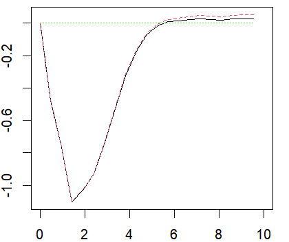
Independent Gaussian perturbations. For independent Gaussian perturbations, we have $\kappa_{i}^{\sigma}=2\sigma^{2}$. We choose $r_{1}=0,r_{2}=3$ and the final minimizer is $\hat{\sigma}=0.18$. Below is the comparison of the centered Besag’s L-function of the fitted model together with the estimated centered L-function from the data.

Figure 8: (a) Black lines corresponds to the estimated centered L-function, green dashed line is the theoretical value of Poisson point process while red line represents the theoretical value of the fitted independently perturbed lattice with Gaussian random variables with standard deviation $\sigma=0.18$. (b) Global envelope test for the fitted i.i.d perturbed Gaussian lattice.

The periodic peaks that occur at the tail of the theoretical centered $L$-function in Figure 8 are typical for independently perturbed lattices. Note that this phenomenon is less visible if we increase the variance in the model. However, the estimated standard deviation is low enough to preserve this property. To verify the validity of the model, we performed a global envelope test based on [28] (see Figure 8, (b)). Due to these tail peaks and also suppression of the variance caused by hyperuniformity of the model, the independently perturbed lattice by Gaussian random variables is not a good approximation of the data. The need of a more flexible model motivates the subsequent paragraph.

Dependent Gaussian perturbations. Similarly as with the independent Gaussian perturbation, we used the minimum contrast method based on the $K$-function of Lemma 1 and (4.3) to estimate the parameters in the dependent Gaussian perturbation model resulting in $\hat{\sigma}=0.3,\hat{r}=2.5$ and $\hat{\gamma}=2$. The tail peaks were less visible in comparison to the i.i.d case. However, the global envelope test rejected this model. The reason is the low empirical variance of the $L$-function in the region $r\in(0.5,1.5)$ (This is already visible at Figure 8).

For this reason, we performed the second step of the optimization procedure. Based on previous simulations, we compute the empirical variance of the centered $L$-function for each $r\in[0,3]$. Let us denote this function by $\hat{l}(r)$. The second optimization step is then based on a weighted function

$$D(\theta)=\int_{r_{1}}^{r_{2}}\frac{1}{\sqrt{\hat{l}(r)}}\left|\left(\sum_{i\in\mathbb{Z}^{3}\setminus\{0\}}P_{3}(r^{2}/\kappa^{\theta}_{i},|i|^{2}/\kappa^{\theta}_{i})\right)^{1/4}-\hat{K}_{NiTi}(r)^{1/4}\right|^{2}\mathrm{d}r,$$

With $r_{1}=0.2$ and $r_{2}=2$, we arrive at the estimates $\hat{\sigma}=0.32,\hat{r}=2.5$ and $\hat{\gamma}=2$. The global envelope test (see Figure 9) for the fitted dependent perturbed Gaussian lattice was performed resulting in $p$-value $24,4\%$ which implies a good fit.

Figure 9: (a) Black lines corresponds to the estimated centered L-function, green dashed line is the theoretical value of Poisson point process while red line represents the theoretical value of the fitted dependently perturbed lattice with parameters $\hat{\sigma}=0.32,\hat{r}=2.5$ and $\hat{\gamma}=2$ (b) Global envelope test for the fitted dependent perturbed Gaussian lattice. The corresponding p-value obtained by the global area rank envelope test is $24,4\%$

Finally, we compare the original data with the simulated point pattern from the fitted model in Figure 10.

Figure 10: Left is the original dataset, right is the simulated lattice perturbed by a Gaussian random field given by (4.2) with fitted parameters $\hat{\sigma}=0.32,\hat{r}=2.5$ and $\hat{\gamma}=2$.

5 Conclusion

When analyzing spatial data that exhibit a high degree of regularity, it is natural to investigate the growth of number variance relative to a Poisson point process. Hyperuniform models are particularly relevant when there are theoretical or physical reasons to expect suppressed large-scale fluctuations. However, reliable empirical confirmation of hyperuniformity from a single finite dataset is often challenging. In this context, perturbed lattices provide a flexible parametric framework for modelling regular point patterns, regardless of whether hyperuniformity can be shown.

From a computational perspective, models based on perturbed lattices are easy to simulate and calibrate. Independently perturbed lattices already offer a simple baseline model, although their rigid spectral structure, including visible Bragg peaks, may limit their descriptive power. Introducing correlations among the perturbations substantially increases modelling flexibility. In particular, dependent Gaussian perturbations are attractive in practice because their second-order characteristics, including the $K$-function, are available in explicit form.

Compared to classical Gibbs point processes, perturbed-lattice models avoid the need to specify and estimate an interaction potential and do not involve an intractable normalizing constant, leading to significant computational advantages. Gibbs models nevertheless remain a powerful and flexible tool for modelling repulsive data, especially when detailed control over interaction structure is required. The perturbed-lattice framework should therefore be viewed as a complementary approach that is particularly appealing when computational efficiency and analytical tractability are important considerations.

6 Future extension

Central limit theorems for cell characteristics of a tessellation based on the NiTi data. First, we should find a suitable model for the distribution of the radii $r$ (e.g. by following the hierarchical approach by [34]) to construct a marked perturbed lattice $\Xi_{m}=\{(x,m),x\in\Xi,r\geq 0\}=\{(x_{i},r_{i})_{i\in\mathbb{Z}^{3}}\}$, where the cell generated by a marked point $(x,r)$ is

$$C^{\rho}((x,r),\Xi_{m})=\bigcap_{i\in\mathbb{Z}^{3}}\{y\in\mathbb{R}^{3}:\rho(y,(x,r))\leq\rho(y,(x_{i},r_{i}))\}.$$

The common choices of the function $\rho$ are listed below

• Voronoi tessellation: $\rho(y,(x,r))=|y-x|$

• Laguerre tessellation: $\rho(y,(x,r))=|y-x|^{2}-r^{2}$

• Johnson-Mehl tessellation: $\rho(y,(x,r))=|y-x|-r$

If $K_{\mathbf{0}}^{\rho}(\Xi_{m})$ is the cell generated by the typical point of $\Xi_{m}$ (in the Palm sense), we are interested in the estimation of $\mathbb{E}\xi(K_{\mathbf{0}}^{\rho})$ where $\xi$ is some function on closed sets (diameter, volume, etc.)

$$H_{n}=\sum_{i\in\mathbb{Z}^{3}\cap W_{n}}\xi(C((x_{i},r_{i}),\Xi_{m}))\cdot\text{weight}_{i},$$

where the weights are chosen reasonably so that the estimator $H_{n}$ is (asymptotically) unbiased and consistent. The stabilization methods and mixing properties of the perturbation field could then be used to show that

$$\frac{H_{n}-\mathbb{E}H_{n}}{\sqrt{\sigma_{n}}}\xrightarrow[n\to\infty]{\mathcal{D}}N(0,\sigma^{2}_{\xi}),$$

where $\sigma_{n}=\textbf{var}|\Xi\cap W_{n}|$. This asymptotic study should be carried out in a separate paper.

References

- [1] Björklund, M. and Hartnick, T. (2024): Hyperuniformity and non-hyperuniformity of quasicrystals, Math. Ann. 389, 365–426.
- [2] Bradley, R. C. (2002): On positive spectral density functions. Bernoulli 8(2), 175–193.
- [3] Chiu, S. N., Stoyan, D., Kendall, W. S. and Mecke, J. (2013): Stochastic geometry and its applications. Wiley Series in Probability and Statistics. John Wiley & Sons.
- [4] Coste, S. (2021): Order, fluctuations, rigidities. Available here.
- [5] Daley, D. J. and Vere-Jones, D. (2003): An Introduction to the Theory of Point Processes: Volume I: Elementary Theory and Methods, Second Edition. Springer, New York.
- [6] Davydov, Yu. (1970): Invariance principle for stationary processes, Theory Prob. Appl. 15(3), 498–509.
- [7] Dereudre, D., Flimmel, D. Huesmann, M. and Leblé, T. (2024): (Non)-hyperuniformity of perturbed lattices. Preprint. arxiv.org/pdf/2405.19881.
- [8] Dereudre, D. and Flimmel, D. (2024): Non-hyperuniformity of Gibbs point processes with short-range interactions, J. Appl. Probab. 61 (4), 1380–1406.
- [9] Doukhan, P. (1994): Mixing: Properties and Examples, Lecture Notes in Statistics vol. 85, Springer-Verlag.
- [10] Fry, N. (1979): Random point distributions and strain measurement in rocks. Tectonophysics, vol. 60, 89–105.
- [11] Gabrielli, A. (2004): Point processes and stochastic displacement fields, Phys. Rev. E. 70(6), 066131.
- [12] Ghosh, S. and Lebowitz, J. (2017): Fluctuations, large deviations and rigidity in hyperuniform systems: a brief survey, Indian J. Pure Appl. Math. 48(4), 609–631.
- [13] Hawat, D., Gautier, G., Bardenet, R. et al. (2023): On estimating the structure factor of a point process, with applications to hyperuniformity, Stat. Comput. 33 (61).
- [14] Hof, A. (1995): Diffraction by aperiodic structures at high temperatures, J. Phys. A 28, 57–62.
- [15] Jalowy, J and Stange, H. (2025): Box-covariances of hyperuniform point processes. Preprint. arxiv.org/abs/2506.13661.
- [16] Jiao, Y., Lau, T. and Hatzikirou, H. et al (2014): Avian photoreceptor patterns represent a disordered hyperuniform solution to a multiscale packing problem, Phys. Rev. E 89.
- [17] Kanter, M. (1975): Stable Densities Under Change of Scale and Total Variation Inequalities, Ann. Probab. 3(4), 697–707.
- [18] Klatt, M. A., Kim, J. and Torquato, S. (2020): Cloaking the underlying long-range order of randomly perturbed lattices, Phys. Rev. E 101.
- [19] Klatt, M. A., Last, G. and Henze, N. (2024): A genuine test for hyperuniformity. Preprint. arxiv.org/abs/2210.12790.
- [20] Klatt, M. A., Last, G., Lotz, L. and Yogeshwaran D. (2025): Invariant transports of stationary random measures: asymptotic variance, hyperuniformity, and examples. Preprint. arxiv.org/pdf/2506.05907
- [21] Lachièze-Rey, R. and Yogeshwaran, D. (2024): Hyperuniformity and optimal transport of point processes. Preprint. arxiv.org/abs/2402.13705.
- [22] Lachièze-Rey, R. (2025): Hyperuniform random measures, transport and rigidity. Preprint. arxiv.org/abs/2510.18392.
- [23] Lebedev, N.N. and Silverman, R.A. (1972): Special Functions and Their Applications. Dover Books on Mathematics. Dover Publications.
- [24] Li, Y., Shanchao, Y. and Chengdong, W. (2011): Some inequalities for strong mixing random variables with applications to density estimation, Stat. Probab. Lett. 81, 250–258.
- [25] Mastrilli, G., Błaszczyszyn, B. and Lavancier, F. (2024): Estimating the hyperuniformity exponent of point processes. Preprint. arxiv.org/pdf/2407.16797.
- [26] Mayer, A., Balasubramanian, V., Mora, T. and Walczak, A. M. (2015): How a well-adapted immune system is organized, Proc. Nat. Acad. Sci. E 112, 5950–5955.
- [27] Møller, J. and Waagepetersen, R. P. (2004): Statistical Inference and Simulation for Spatial Point Processes, 2nd edition, Chapman & Hall/CRC.
- [28] Myllymäki, M., Mrkvička, T., Grabarnik, P., Seijo, H. and Hahn, U. (2017): Global envelope tests for spatial processes. J. R. Stat 79(2), 381–404
- [29] Peebles, P. J. E. (1993): Principles of Physical Cosmology, Princeton University Press, Princeton.
- [30] Peres, Y. and Sly, A. (2014): Rigidity and tolerance for perturbed lattices. Preprint. arxiv.org/pdf/1409.4490.
- [31] Petrich, L., Staněk, J., Wang, M. et al. (2019): Reconstruction of Grains in Polycrystalline Materials From Incomplete Data Using Laguerre Tessellations, Microsc. Microanal. 25(3), 743–752.
- [32] Pratt, J. W. (1960): On Interchanging Limits and Integrals, Ann. Math. Statist. 31(1), 74–77
- [33] Rajala, T., Redenbach, C., Särkkä, A. and Sormani, M. (2018): A review on anisotropy analysis of spatial point patterns. Spatial Statistics 28, 141–168.
- [34] Seitl, F., Møller, J. and Beneš, V. (2022): Fitting three-dimensional Laguerre tessellations by hierarchical marked point process models, Spat. Stat. 51.
- [35] Stein, E. M. and Weiss, G. (1971): Introduction to Fourier analysis on Euclidean spaces, Volume 1. Princeton university press.
- [36] Torquato, S. and Stillinger, F. H. (2003): Local density fluctuations, hyperuniformity, and order metrics, Phys. Rev. E 68, 041113.
- [37] Torquato, S. (2016): Hyperuniformity and its generalizations, Phys. Rev. E 94, 022122.
- [38] Torquato, S. (2018): Hyperuniform states of matter, Phys. Rep. 745, 1–95.
- [39] Yakir, O. (2021): Fluctuations of linear statistics for Gaussian perturbations of the lattice , J. Stat. Phys. 182, Paper No. 58.
- [40] Yakir, O. (2022): Recovering the lattice from its random perturbations, Int. Math. Res. Not. IMRN 8, 6243–6261.