Pair correlations of one-dimensional model sets
and monstrous covariograms of Rauzy fractals

Abstract.

The averaged distance structure of one-dimensional regular model sets is determined via their pair correlation functions. The latter lead to covariograms and cross covariograms of the windows, which give continuous functions in internal space. While they are simple tent-shaped, piecewise linear functions for intervals, the typical case for inflation systems leads to convolutions of Rauzy fractals, which are difficult to compute. In the presence of an inflation structure, an alternative path is possible via the exact renormalisation structures of the pair correlation functions. We introduce this approach and derive two concrete examples, which display an unexpectedly complex and wild behaviour.

1. Introduction

The distance structure of lattices and periodic point sets is efficiently summarised in the corresponding theta series, which are well studied and understood, and have close connections with modular forms [22]. Much less is known for aperiodic point sets, even for the most popular ones such as the Fibonacci or the silver mean chain. It is questionable to what extent individual theta series are meaningful, as no two members of the Fibonacci hull would have the same series, and similarly for all other (regular) model sets.

A natural question would then be what the averaged distance structure is, where the average is taken over all elements of the hull with a point at 0. This average is well defined and can often be determined, at least in principle, from one element of the hull. For regular model sets, which are particularly nice cut-and-project sets, the answer is then given in terms of (sums of) pair correlation functions. The latter, in turn, lead to covariograms of the coding windows, or cross covariograms between different windows. These are always continuous functions in internal space, which sounds nice and easy. If the windows are simple polygons, one indeed obtains decent functions. Nevertheless, no clear relation to aperiodic analogues of theta series has materialised so far, despite several efforts in this direction [1, 11, 21, 34].

In view of this, potential insight might come from investigating some less prominent examples that are nevertheless somehow typical. Indeed, even within the class of one-dimensional inflation tilings, windows of Rauzy fractals are ubiquitous, but have not been studied from this point of view. One reason certainly is the obstacle of computing the covariogram of a Rauzy fractal, which already in one dimension tends to be a Cantorval [10]. The covariograms are continuous functions (being convolutions of two functions that are both $L^{1}$ and $L^{\infty}$), with a behaviour that is somewhat reminiscent to that of a Weierstrass monster.

In fact, until recently, hardly any reliable technique for computing these functions was known. Within the class of inflation point sets, the identification of an exact renormalisation scheme for the pair correlation functions in [9, 29] opens the door to some efficient and exact calculations, as we will demonstrate by way of two examples (for more, see [26]). The crucial connection comes from the uniform distribution property of the model set points within the windows, after their lift via the $\star$-map. Consequently, the renormalisation scheme permits the calculation of the (cross) covariograms at a dense set of points, which is enough for the illustration of a continuous function.

This looks like a maybe tedious, but ultimately easy thing to do — until one actually does it. Indeed, the spiky behaviour of the covariograms turns out to be unexpectedly wild, and the convergence of the approximants is surprisingly slow — at least in some examples. It is thus the goal of this paper to introduce the problem and method via some characteristic examples, and to demonstrate that this is a fractal phenomenon worth further study.

This paper is organised as follows. In Section 2, we set the scene and introduce the key concepts and notions around covariograms, cut-and-project sets and pair correlation functions. In the main Section 3, we then derive the results for two binary inflation systems. The first is based on the silver mean inflation factor, $\lambda=1+\sqrt{2}$, and the second on its square. A central block will be the explicit derivation of the exact renormalisation equations, and how they are used to approach the (cross) covariograms.

2. Preliminaries

Let us begin by recalling some concepts and notions; see [13] for general background.

Definition 2.1.

Let $W\subset\mathbb{R}\hskip 0.5pt^{m}$ be a non-empty compact set. We define the covariogram of $W$ for almost all $x\in\mathbb{R}\hskip 0.5pt^{m}$ as

$$\mathrm{cvg}\hskip 0.5pt_{W}(x)\,\mathrel{\mathop{:}}=\,\operatorname{\mathrm{vol}}\hskip 0.5pt\bigl(W\cap(x+W)\bigr)\,=\,\big(\mathbf{1}_{-W}\ast\mathbf{1}_{W}\big)(x)\hskip 0.5pt,$$

where $\mathbf{1}_{W}$ is the characteristic function of $W$, and $\ast$ stands for the usual convolution of two functions $f,\hskip 0.5ptg\in L^{1}(\mathbb{R}\hskip 0.5pt^{m})$ as given by

$$(f\ast g)(x)\,=\int_{\mathbb{R}\hskip 0.5pt^{m}}f(y)\hskip 0.5ptg(x-y)\mathop{}\!\mathrm{d}y\hskip 0.5pt,$$

with the usual understanding that this is well defined for almost all $x\in\mathbb{R}\hskip 0.5pt^{m}$.

Arguably, this is most famously known in relation to the covariogram problem whether the covariogram of a convex body in $\mathbb{R}\hskip 0.5pt^{m}$ determines the body uniquely, up to translations and reflections. The answer is positive for convex polytopes when $m\leqslant 3$; see [20]. Variations of this problem exist and apply to our setting, such as determining when two model sets share the same covariogram and the corresponding inverse problem [12].

Before turning our attention to the realm of model sets, we briefly recall and collect various properties of a covariogram that immediately follow from its definition, some usual inequalities, and elementary change of variables arguments; see [13, 26] for further references.

Proposition 2.2.

Let $W,W^{\prime}\subset\mathbb{R}\hskip 0.5pt^{m}$ be non-empty compact sets. Then,

1. $\mathrm{cvg}\hskip 0.5pt_{W}\in C_{\mathtt{c}}(\mathbb{R}\hskip 0.5pt^{m})$, and $\mathrm{cvg}\hskip 0.5pt_{W}$ is an even function,

2. $\mathrm{supp}(\mathrm{cvg}\hskip 0.5pt_{W})\subseteq W\!-W\mathrel{\mathop{:}}=\{x-y:x,y\in W\}$,

3. $W\hskip-0.5pt\subseteq W^{\prime}$ implies $\mathrm{cvg}\hskip 0.5pt_{W}(x)\,\leqslant\,\mathrm{cvg}\hskip 0.5pt_{W^{\prime}}(x)$ for all $\in\mathbb{R}\hskip 0.5pt^{m}$,

4. $\mathrm{cvg}\hskip 0.5pt_{W}$ is Fourier transformable, and one has, for all $x\in\mathbb{R}\hskip 0.5pt^{m}$,

   $$\widehat{\mathrm{cvg}\hskip 0.5pt_{W}}(x)\,=\,\bigl|\widehat{\mathbf{1}_{W}}(x)\bigr|^{2}\hskip 0.5pt,$$

5. for all $b\in\mathbb{R}\hskip 0.5pt^{m}$ and all $\lambda\in\mathbb{R}\hskip 0.5pt$ with $\lambda>0$, one has

   $$\mathrm{cvg}\hskip 0.5pt_{W+\hskip 0.5ptb}(x)\,=\,\mathrm{cvg}\hskip 0.5pt_{W}(x)\hskip 0.5pt,\quad\mbox{and}\quad\,\mathrm{cvg}\hskip 0.5pt_{\lambda W}(x)\,=\,\lambda\hskip 0.5pt\hskip 0.5pt\mathrm{cvg}\hskip 0.5pt_{W}\Big(\frac{\raisebox{-2.0pt}{$x$}}{\raisebox{0.5pt}{$\lambda$}}\Big),$$

6. if $\mathrm{int}(W)\cap\mathrm{int}(\mathrm{W^{\prime}})=\varnothing$ with $\operatorname{\mathrm{vol}}(\partial W)=\operatorname{\mathrm{vol}}(\partial W^{\prime})=0$, one has

   $$\mathrm{cvg}\hskip 0.5pt_{W\hskip 0.5pt\cup\hskip 0.5ptW^{\prime}}(x)\,=\,\mathrm{cvg}\hskip 0.5pt_{W}(x)+\mathrm{cvg}\hskip 0.5pt_{W^{\prime}}(x)+\bigl(\mathbf{1}_{-W}\ast\mathbf{1}_{W^{\prime}}\bigr)(x)+\bigl(\mathbf{1}_{-W}\ast\mathbf{1}_{W^{\prime}}\bigr)(-x)$$

   for almost every $x\in\mathbb{R}\hskip 0.5pt^{m}\hskip-0.5pt$. ∎

Clearly, the complexity of determining the covariogram of a given set $W$ depends on its structure. We are interested in finding the covariograms of so-called Rauzy fractals. They are solutions of an iterated function system and are intimately related to Pisot substitutions and their description as model sets. We briefly summarise this connection in what follows, and refer the reader to [13] for further details and to [32, 35, 36] for deeper connections.

Let $\mathcal{A}$ be a finite set of $n$ symbols, called an alphabet. A substitution rule $\varrho$ is a map that sends each element of $\mathcal{A}$ (a letter) to a non-empty concatenation of finitely many letters (a word), and extends to all (bi-infinite) words by the endomorphism property. To every substitution rule $\varrho$, one can assign the substitution matrix $M_{\varrho}\in\mathrm{Mat}(n,\,\mathbb{Z}\hskip 0.5pt)$ with entries

$$\bigl(M_{\varrho}\bigr)_{ij}\hskip 0.5pt=\,\text{number of letters of type $i$ in }\varrho(j)\hskip 0.5pt,$$

where we have fixed a numbering of the letters of $\mathcal{A}$. A substitution $\varrho$ is primitive if its substitution matrix $M_{\varrho}$ is primitive. By iterating a primitive substitution rule, starting with a letter from the alphabet (or, more generally, with a legal word [13, Def. 4.5]), we obtain for (a suitable power of) the substitution a (bi)-infinite fixed point — a sequence of letters from the alphabet which is invariant under the action of (the power of) the substitution rule.

Since the substitution matrix is a non-negative matrix, via standard Perron–Frobenius (PF) arguments [13, Ch. 2.4], it provides insight into various properties of $\varrho$. In particular, if a primitive substitution is additionally a Pisot substitution, meaning the PF eigenvalue of $M_{\varrho}$ is a Pisot–Vijayaraghavan (PV) number and the characteristic polynomial is irreducible, the substitution leads to a tiling of the real line by assigning a closed interval to each letter whose (natural tile) length is proportional to an entry of the left PF eigenvector of $M_{\varrho}\hskip 0.5pt$. These intervals are called prototiles. Then, the PF eigenvalue of $M_{\varrho}$ gives the inflation factor $\lambda$ of the induced (geometric) inflation rule. In this setting, it is natural to work with the displacement matrix $T_{\varrho}$, which is a set-valued analogue of the substitution matrix with entries

$$\bigl(T_{\varrho}\bigr)_{ij}\,=\,T_{ij}\,=\,\left\{\mbox{relative positions of tiles of type $i$ in supertile }\varrho(j)\right\}\hskip 0.5pt,$$

and one has $(M_{\varrho})_{ij}=\operatorname{\mathrm{card}}(T_{ij})$. Placing a control point on the left endpoint of each tile, we can understand the fixed point of a given substitution as a collection of point sets assigned to each letter. If we collect all control points of tiles of type $i$, we obtain a Delone set $\varLambda_{i}\subset\mathbb{R}\hskip 0.5pt$. The set of all control points will be denoted by $\varLambda$. It satisfies

$$\varLambda\,=\bigcup_{k=1}^{n}\varLambda_{k}$$

and the union is disjoint. Since one considers a tiling of the real line described as a fixed point of a Pisot substitution (inflation) rule $\varrho$ with $n$ letters (prototiles) with the inflation factor $\lambda$, this is reflected on the level of the control points as

(2.1) $$\varLambda_{i}\,=\,\bigcup_{j=1}^{n}\,\lambda\varLambda+T_{ij}\,=\,\bigcup_{j=1}^{n}\,\bigcup_{t\in T_{ij}}\lambda\varLambda_{j}+t\hskip 0.5pt,$$

where, again, the unions are disjoint. Note that the RHS, viewed as a mapping between $n$-tuples of Delone sets, does not define a contraction with respect to any natural metric. Consequently, a characterisation of the solution space of (2.1) is difficult. We are not aware of any general result in this direction.

If the alphabet is binary and $\lambda$ is a PV number, the sets $\varLambda_{i}$ are regular model sets [23]. For larger alphabets, this problem is known under the name Pisot substitution conjecture. It is unclear whether or not it should hold, but all known examples with irreducible characteristic polynomial of the substitution matrix satisfy it. We refer the reader to [2] for a summary on the Pisot substitution conjecture, to [17] for various families for which the conjecture has been verified, and to [16] for an extensive computer search for a counterexample.

Model sets are special cases of cut-and-project sets with nice properties, both arising from cut-and-project schemes; compare [32, 33].

Definition 2.3.

A cut-and-project scheme (CPS) is a triple $(\mathbb{R}\hskip 0.5pt^{d},\,H,\,\mathcal{L})$ consisting of $\mathbb{R}\hskip 0.5pt^{d}$ (direct/physical space) and a locally compact Abelian group (LCAG) $H$ (internal space), together with a discrete co-compact subgroup — a lattice — $\mathcal{L}\subset\mathbb{R}\hskip 0.5pt^{d}\times H$ and the natural projections $\pi:\mathbb{R}\hskip 0.5pt^{d}\times H\to\mathbb{R}\hskip 0.5pt^{d}$ and $\pi_{\text{int}}:\mathbb{R}\hskip 0.5pt^{d}\times H\to H$ enjoying the following properties:

1. The restriction $\pi|_{\mathcal{L}}$ is one-to-one.

2. The image $\pi_{\text{int}}(\mathcal{L})$ is dense in $H$.

Given a CPS $(\mathbb{R}\hskip 0.5pt^{d},\,H,\,\mathcal{L})$, we set $L=\pi(\mathcal{L})$, which is a subgroup of $\mathbb{R}\hskip 0.5pt^{d}$. The first condition in the definition of a CPS implies the existence of a mapping $\star:L\to H$, called the $\star$-map (known as the star map), defined by $\star=\pi_{\text{int}}\circ(\pi|_{\mathcal{L}})^{-1}$. If $H=\mathbb{R}\hskip 0.5pt^{m}$, the CPS is called Euclidean. We summarise a CPS via the diagram

$$\begin{array}[]{ccccc@{}l}\mathbb{R}\hskip 0.5pt^{d}&\xleftarrow{\;\;\;\pi\,\hskip 0.5pt\;\;\;}&\mathbb{R}\hskip 0.5pt^{d}\hskip-0.5pt\hskip-0.5pt\times\hskip-0.5pt\hskip-0.5ptH&\xrightarrow{\;\>\pi_{\text{int}}\;\>}&H&\\ \cup&&\cup&&\cup&\hskip-8.61108pt\raisebox{1.0pt}{\text{\scriptsize dense}}\\ \pi(\mathcal{L})&\xleftarrow{\;\hskip 0.5pt1-1\;\hskip 0.5pt}&\mathcal{L}&\xrightarrow{\qquad}&\hskip 0.5pt\pi_{\text{int}}(\mathcal{L})&\\ \|&&&&\|&\\ L&\lx@intercol\hfil\xrightarrow{\qquad\quad\quad\ \star\quad\quad\qquad}\hfil\lx@intercol&{L}^{\star\hskip-0.5pt}&\end{array}$$

as usual. With the $\star$-map, we can now define a model set. We refer the reader to [13, Sec. 7] and [33] for further discussions of model sets and their properties.

Definition 2.4.

Given a CPS $(\mathbb{R}\hskip 0.5pt^{d},\,H,\,\mathcal{L})$ and an arbitrary, relatively compact set $W\subset H$, we denote by $\mbox{\Large$\curlywedge$}(W)$ the set

$$\mbox{\Large$\curlywedge$}(W)\,\mathrel{\mathop{:}}=\,\{x\in L:x^{\star}\in W\}\hskip 0.5pt,$$

which we call a cut-and-project set. If $W$ has non-empty interior, $\mbox{\Large$\curlywedge$}(W)$, or any translate $t+\mbox{\Large$\curlywedge$}(W)$ with $t\in\mathbb{R}\hskip 0.5pt^{d}$, is called a model set. When the boundary $\partial W$ has zero Haar measure in $H$, the model set is called regular.

Now, one version of the Pisot substitution conjecture states that, if we have a set of control points $\varLambda_{i}$ of a tiling arising from a Pisot substitution, we can find a suitable LCAG $H$ and relatively compact sets $W_{i}\subset H$ with non-empty interior such that $\varLambda_{i}=\mbox{\Large$\curlywedge$}(W_{i})$ up to a set of zero density. We restrict ourselves to unimodular substitutions, which means we have $\lvert\det(M_{\varrho})\rvert=1$. Under this additional assumption, we obtain a Euclidean CPS [13, 36]. This is also plausible from the results in [18], which establish an appropriate connection to a minimal rotation on a torus, and thus a fully Euclidean embedding.

Since one can, without loss of generality, assume that all $\varLambda_{i}$ belong to the ring of integers $\mathcal{O}_{\mathbb{Q}(\lambda)}$ of the algebraic number field $\mathbb{Q}(\lambda)$, where $\lambda$ is the inflation factor, we employ a Minkowski embedding of $\mathcal{O}_{\mathbb{Q}(\lambda)}$ to obtain the lattice $\mathcal{L}$. The projection $\pi$ on its first coordinate gives the control points, whereas the remaining ones give the projection $\pi_{\mathrm{int}}$ into the internal space, which is $\mathbb{R}\hskip 0.5pt^{m}$ (if $\lambda$ is of degree $n$, then $m=n-1$). Now, for the windows, one considers the $\star$-image of Eq. (2.1) and its closure. Then, with $W_{i}\mathrel{\mathop{:}}=\overline{\varLambda^{\star}_{i}}$, we obtain

(2.2) $$W_{i}\,=\bigcup_{j=1}^{n}\bigcup_{t\in T_{ij}}\lambda^{\star}W_{j}+t^{\star},$$

which is an iterated function system on the space $\big(\mathcal{K}(\mathbb{R}\hskip 0.5pt^{m})\big)^{n}$ of all $n$-tuples of non-empty compact subsets of $\mathbb{R}\hskip 0.5pt^{m}$ equipped with Hutchinson’s metric; see [15] for details. Since the RHS defines a contraction, by Hutchinson’s theorem [24] (a version of the Banach’s contraction principle), one has a unique solution. The resulting sets are called Rauzy fractals and have been studied extensively; see for example [4, 14, 35]. Some of their properties include the fact that they are topologically regular (i.e., no isolated points) and compact sets of positive measure with a (usually) fractal boundary [19]. If the internal space is one-dimensional, one can even speak of the Rauzy fractal being a Cantorval, for which we refer the reader to [10]. Let us summarise some useful properties of Rauzy fractals as follows.

Proposition 2.5 ([36, Cor. 6.66]).

Let $\{W_{i}:1\leqslant i\leqslant n\}$ be the unique solution of (2.2), as obtained from a unimodular Pisot substitution. Then, the following properties hold.

• All $W_{i}$ have positive Lebesgue measure.

• In the IFS (2.2), the unions on the right-hand side are measure disjoint.

• The boundaries $\partial W_{i}$ have zero Lebesgue measure.

• The sets $W_{i}$ are topologically regular, i.e., they are the closures of their interiors and thus contain no isolated points.

• The interiors of the $W_{i}$ are disjoint. ∎

In this context, we also refer the reader to further pioneering works on the geometry of unimodular Pisot substitutions, such as [5, 25, 37].

Since the topology of Rauzy fractals can be extremely complicated, such as having infinitely many connected components with non-integer boundary dimensions [35], their covariograms are, by standard means, impossible to obtain. On the other hand, since Rauzy fractals correspond (in some sense) to fixed points of substitutions, we have an additional tool at hand — the pair correlation functions. For a model set $\varLambda=\bigcup_{j=1}^{n}\varLambda_{j}$, let

$$\nu_{ij}(y)\,\mathrel{\mathop{:}}=\lim_{r\to\infty}\frac{1}{\operatorname{\mathrm{card}}(\varLambda^{(r)})}\sum_{\begin{subarray}{c}x\in\varLambda^{(r)}_{i}\\ x+y\in\varLambda_{j}\end{subarray}}\!\!1$$

denote the relative frequency of a $2$-point patch consisting of a control point of type $i$ on the left and a control point of type $j$ on the right with distance $y\in\varLambda_{j}-\varLambda_{i}$, where a negative $y$ flips the role of left and right. This quantity exists uniformly by the uniform distribution property of model sets [13, Thm. 7.3]. By applying the $\star$-map, with $\varLambda^{(r)}_{j}=\varLambda_{j}\cap B_{r}(0)$, we obtain the representation

$$\nu_{ij}(y)\, =\lim_{r\to\infty}\frac{1}{\operatorname{\mathrm{card}}(\varLambda^{(r)})}\sum_{\begin{subarray}{c}x^{\star}\in(\varLambda^{(r)}_{i})^{\star}\\ (x+y)^{\star}\in W_{j}\end{subarray}}\!\!1\;=\;\frac{1}{\text{vol}(W)}\int_{\mathbb{R}\hskip 0.5pt^{n-1}}\mathbf{1}_{W_{i}}(z)\,\mathbf{1}_{W_{j}}(z+y^{\star})\,\mathop{}\!\mathrm{d}z$$

$$=\,\frac{\big(\mathbf{1}_{-W_{i}}*\mathbf{1}_{W_{j}}\big)(y^{\star})}{\text{vol}(W)}\,=\mathrel{\mathop{:}}\,g_{ij}(y^{\star})\hskip 0.5pt,$$

where the second equality in the first line holds by Weyl’s theorem on uniform distribution [28, 13]. Up to a factor of $\operatorname{\mathrm{vol}}(W)^{-1}$, the functions $g_{ij}$ are precisely the covariograms of Definition 2.1, so

(2.3) $$\nu_{ij}(x)\,=\,\begin{cases}\frac{1}{\operatorname{\mathrm{vol}}(W)}\,\bigl(\boldsymbol{1}_{-W_{i}}\ast\boldsymbol{1}_{W_{j}}\bigr)(x^{\star})\hskip 0.5pt,&\mbox{if}\ x\in\varLambda_{j}-\varLambda_{i}\hskip 0.5pt,\\ 0\hskip 0.5pt,&\mbox{otherwise}.\end{cases}$$

Remark 2.6.

Recall that, by Proposition 2.2, the covariogram is a continuous function. Moreover, if $x\in\varLambda_{j}-\varLambda_{i}$, the points $x^{\star}$ are dense in $W_{j}-W_{i}$, by definition of the CPS, and uniformly distributed by Weyl’s theorem [28, 13]. Therefore, plotting the covariogram on a sufficiently large sample of these $x^{\star}$, one expects a good illustration of the continuous function and its behaviour, though care is definitely required in view of the vast range of phenomena that are possible in the realm of continuous functions. $\Diamond$

By realising the covariogram of the window as the autocorrelation function of the model set, we can circumvent issues with the window in internal space, and instead work with the renormalisation relations for $\nu_{ij}$. These techniques were introduced in [7] and further developed and used, for example, in [9, 29, 31]. We recall the main result that profits from the inflation structure and enables computing these quantities.

Proposition 2.7 ([29, Prop. 2.2.1] and [9, Lemma 3.16]).

Let $\{\varLambda_{i}\}_{i=1}^{n}$ be a fixed point of a primitive geometric inflation $\varrho$ with inflation factor $\lambda>1$ arising from a substitution over an $n$-letter alphabet. Then, the pair correlation functions $\nu_{ij}$ exist, and satisfy the exact renormalisation equations

$$\nu_{ij}(x)\,=\,\frac{\raisebox{-2.0pt}{$1$}}{\raisebox{0.5pt}{$\lambda$}}\sum_{k,\ell=1}^{n}\,\sum_{r\in T_{ik}}\,\sum_{s\in T_{j\ell}}\nu_{k\ell}\left(\frac{\raisebox{-2.0pt}{$x+r-s$}}{\raisebox{0.5pt}{$\lambda$}}\right),$$

where $T_{\varrho}=(T_{ij})$ is the displacement matrix of the inflation $\varrho$. ∎

As $\lambda>1$, the arguments of the $\nu_{ij}$ on the RHS of the equations in Proposition 2.7 are generally smaller in modulus than those on the LHS. Since $\nu_{ij}(x)=0$ for all $x\notin\varLambda_{j}-\varLambda_{i}$, the system of equations splits naturally into a self-consistent part, which closes on itself, and the recursive part. As the correlation functions $\nu_{ij}$ satisfy the renormalisation relations, their counterparts $g_{ij}$ satisfy the same equations on a subset of $\mathbb{R}\hskip 0.5pt^{m}$ given by the $\star$-image of $\varLambda_{j}-\varLambda_{i}$. These equations can also be derived without prior knowledge of the renormalisation equations from Proposition 2.7. It suffices to know the IFS for the windows, Eq. (2.2), which gives some kind of a dual to the equations from Proposition 2.7. Indeed, the IFS can be turned into a set of equations for the characteristic functions of the windows. These, in turn, induce equations for their (cross) covarigrams, which we shall state next. We recall that $\lambda^{\star}$ refers to the linear mapping $y\mapsto\lambda^{\star}y$ in $\mathbb{R}\hskip 0.5pt^{m}$, which satisfies $(\lambda x)^{\star}=\lambda^{\star}x^{\star}$ for all $x\in\mathbb{Q}(\lambda)$.

Proposition 2.8.

Let $\varLambda_{i}=\mbox{\Large$\curlywedge$}(W_{i})$ be a collection of regular model sets arising from a single CPS $(\mathbb{R}\hskip 0.5pt,\,\mathbb{R}\hskip 0.5pt^{m},\,\mathcal{L})$ describing the control points of a fixed point of a unimodular inflation with a PV inflation factor $\lambda$, and with displacement matrix $T_{\varrho}=(T_{ij})$. Then, the functions $g_{\alpha\beta}\mathrel{\mathop{:}}=\boldsymbol{1}_{-W_{\alpha}}\ast\boldsymbol{1}_{W_{\beta}}$ satisfy, for almost all $y\in\mathbb{R}\hskip 0.5pt^{m}$, the relations

$$g_{ij}(y)\,=\,\frac{\raisebox{-2.0pt}{$1$}}{\raisebox{0.5pt}{$\lambda$}}\sum_{k,\hskip 0.5pt\ell=1}^{n}\,\sum_{r\in T_{ik}}\,\sum_{s\in T_{j\ell}}\,g_{k\ell}\bigl(({\lambda^{\star}})^{-1}(y+r^{\star}{-}\hskip 0.5pts^{\star})\bigr)\hskip 0.5pt.$$

Proof.

We recall the properties of the covariogram function from Proposition 2.2 and observe that $\bigl(\boldsymbol{1}_{-\lambda^{\star}\hskip-0.5ptA}\,\ast\,\boldsymbol{1}_{\lambda^{\star}B}\bigr)(y)\,=|\det(\lambda^{\star})|\bigl(\boldsymbol{1}_{-A}\ast\boldsymbol{1}_{B}\bigr)\big(({\lambda^{\star}})^{-1}y\bigr)$ holds for arbitrary compact sets $A,B$, which follows by a standard change of variables argument. We also recall that the unions on the RHS of (2.2) are measure disjoint and their boundary is of Lebesgue measure zero (Proposition 2.5). Then, we obtain

$$g_{ij}(y)\, =\,\bigl(\boldsymbol{1}_{-W_{i}}\,\ast\,\boldsymbol{1}_{W_{j}}\bigr)(y)\,=\,\Bigl(\boldsymbol{1}_{-\bigcup_{k=1}^{n}\bigcup_{r\in T_{ik}}\lambda^{\star}W_{k}+r^{\star}}\,\ast\,\boldsymbol{1}_{\bigcup_{\ell=1}^{n}\bigcup_{s\in T_{j\ell}}\lambda^{\star}W_{\ell}+s^{\star}}\Bigr)(y)$$

$$=\sum_{k,\hskip 0.5pt\ell=1}^{n}\,\sum_{r\in T_{ik}}\,\sum_{s\in T_{j\ell}}\,\lvert\det(\lambda^{\star})\rvert\,\bigl(\boldsymbol{1}_{-W_{k}}\ast\,\boldsymbol{1}_{W_{\ell}}\bigr)\bigl(({\lambda^{\star}})^{-1}(y+r^{\star}{-}\hskip 0.5pts^{\star})\bigr)$$

$$=\,\frac{\raisebox{-2.0pt}{$1$}}{\raisebox{0.5pt}{$\lambda$}}\sum_{k,\,\ell=1}^{n}\,\sum_{r\in T_{ik}}\,\sum_{s\in T_{j\ell}}\,g_{k\ell}\bigl(({\lambda^{\star}})^{-1}(y+r^{\star}{-}\hskip 0.5pts^{\star})\bigr)\hskip 0.5pt,$$

which holds almost everywhere. For the last equality, let us recall that the Pisot property and unimodularity together imply that $\lambda^{-1}=\lvert\det(\lambda^{\star})\rvert$. ∎

We refer the reader to [30] for a brief summary of the non-unimodular setting with LCAG $H$ having a $p$-adic component. Let us turn to concrete examples and explain further details.

3. Binary Alphabet Examples

In this section, we provide some examples of determining the covariograms of Rauzy fractal windows from Pisot substitutions over a binary alphabet. We first construct a model set with a highly irregular window, and implement the renormalisation procedure to calculate the covariogram. Note that in this one-dimensional internal space case, as conjectured in [10, 30], there are two possibilities for the covariogram: a piecewise linear function, arising from interval-type windows, or a ‘spiky’ function, as illustrated in Figure 3 below. The latter arises when the window is a Cantorval. For an example where the internal space is two-dimensional, we refer the reader to [26].

3.1. The sister silver mean tiling

Let us construct the sister silver mean (SSM) chain. Consider the binary alphabet $\mathcal{A}=\{a\hskip 0.5pt,b\}$, and the substitution rule

$$\varrho_{s}\,:\,\begin{cases}a\mapsto bba\hskip 0.5pt,\\ \hskip 0.5ptb\hskip 0.5pt\mapsto ab\hskip 0.5pt,\end{cases}$$

which we abbreviate as $\varrho_{s}=(bba,ab)=\big(\varrho_{s}(a),\varrho_{s}(b)\big)$. Starting with the legal seed $\omega_{(0)}=a|a$, where $|$ denotes the origin, by iteration one obtains a sequence of growing words $\omega_{(n)}$

$$a\hskip 0.5pt|\hskip 0.5pta\xmapsto{\,\varrho_{s}\,}bba\hskip 0.5pt|\hskip 0.5ptbba\xmapsto{\,\varrho_{s}\,}ababbba\hskip 0.5pt|\hskip 0.5ptababbba\xmapsto{\,\varrho_{s}\,}{\dots}\xmapsto{\,\varrho_{s}\,}\omega_{(n)}\xrightarrow{\,n\to\infty\,}\omega\xmapsto{\,\varrho_{s}\,}\omega^{\prime}\xmapsto{\,\varrho_{s}\,}\omega\hskip 0.5pt,$$

which converges, with obvious meaning in the product topology, towards a $2$-cycle of bi-infinite words $\omega,\omega^{\prime}\in\mathcal{A}^{\mathbb{Z}\hskip 0.5pt}$. The left-infinite half is fixed, while the right-infinite half alternates between two words that differ on a set of zero density only. In fact, they form a proximal pair; see [13, Sec. 4.3] for details.

Now, we can move to the geometric description and easily deal with this difference in the cut-and-project description. The substitution matrix of $\varrho_{s}$ is $M_{s}=\big(\begin{smallmatrix}1&1\\ 2&1\end{smallmatrix}\big)$, with PF eigenvalue $\lambda=1+\sqrt{2}$. The left and (statistically normalised) right PF eigenvectors are

(3.1) $$v_{\ell}=\bigl(\sqrt{2},\,1\bigr)\quad\text{ and }\quad v_{r}\,=\,\bigl(\lambda^{-1},\,\lambda^{-1}\hskip 0.5pt\sqrt{2}\,\bigr)^{\top}\hskip 0.5pt=\,\bigl(\lambda-2,\,3-\lambda\,\bigr)^{\top}.$$

Figure 1. Geometric inflation rule for the self-similar SSM tiling.

The $a$ and $b$ prototiles for this choice have length $\sqrt{2}$ and $1$. The inflated $a\hskip 0.5pt$-tile is called the (level-one) $a$-supertile, and, analogously, we have the (level-one) $b\hskip 0.5pt$-supertile. Below, they will be called the $a$ and $b$ supertiles, and denoted by $\overline{a}$ and $\overline{b}$ respectively; the inflation rule is depicted in Figure 1. Denote the set of left endpoints (control points) of tilings corresponding to $\omega$ and $\omega^{\prime}$ by $\varLambda_{\omega}$ and $\varLambda_{\omega^{\prime}}$. These sets are in a natural one-to-one correspondence with $\omega$ and $\omega^{\prime}$, and each has a density of $\tfrac{2+\sqrt{2}\hskip 0.5pt}{4}$. Thus, the discrepancies between the two fixed points form a zero density set; compare [13, Ch. 4].

Denote the sets of control points of the tiles of types $a$ and $b$ by $\varLambda_{a}$ and $\varLambda_{b}$, with $\varLambda=\varLambda_{a}\,\dot{\cup}\,\varLambda_{b}$. By our choice of the control point, it immediately follows that $\varLambda\subset\mathbb{Z}\hskip 0.5pt[\sqrt{2}\,]$, which is the smallest $\mathbb{Z}\hskip 0.5pt\hskip 0.5pt$-module into which we can embed $\varLambda$. The standard Minkowski embedding of $\varLambda\subset\mathbb{Z}\hskip 0.5pt[\sqrt{2}\,]$ gives the lattice $\mathcal{L}=\mathbb{Z}\hskip 0.5pt(1,1)\oplus\mathbb{Z}\hskip 0.5pt(\sqrt{2},-\sqrt{2})$; see [13, Ch. 7] and [27, Thm. 2.13.1] for details. In particular, the $\star$-map is given by the non-trivial Galois automorphism of $\mathbb{Q}(\sqrt{2}\hskip 0.5pt)$, which is $a+b\sqrt{2}\mapsto(a+b\sqrt{2}\hskip 0.5pt)^{\star}=a-b\sqrt{2}$. This gives the Euclidean CPS

(3.2) $$\begin{array}[]{ccccc@{}l}\mathbb{R}\hskip 0.5pt&\xleftarrow{\;\;\;\pi\;\;\;}&\mathbb{R}\hskip 0.5pt\hskip-0.5pt\hskip-0.5pt\times\hskip-0.5pt\hskip-0.5pt\mathbb{R}\hskip 0.5pt&\xrightarrow{\;\>\pi_{\text{int}}\;\>}&\mathbb{R}\hskip 0.5pt&\\ \cup&&\cup&&\cup&\hskip-8.61108pt\raisebox{1.0pt}{\text{\scriptsize dense}}\\ \pi(\mathcal{L})&\xleftarrow{\;\hskip 0.5pt1-1\;\hskip 0.5pt\hskip 0.5pt}&\mathcal{L}&\xrightarrow{\qquad}&\pi_{\text{int}}(\mathcal{L})&\\ \|&&&&\|&\\ L=\mathbb{Z}\hskip 0.5pt[\sqrt{2}\,]&\lx@intercol\hfil\xrightarrow{\qquad\quad\quad\ \star\quad\quad\qquad}\hfil\lx@intercol&{L}^{\star\hskip-0.5pt}=\mathbb{Z}\hskip 0.5pt[\sqrt{2}\,]&\end{array}$$

By construction, $\pi_{\text{int}}(\mathcal{L})$ is dense in internal space. From a CPS of the form (3.2), we can construct a regular model set, with suitable $W\subset\mathbb{R}\hskip 0.5pt$, as

$$\mbox{\Large$\curlywedge$}(W)\,\mathrel{\mathop{:}}=\,\{x\in L:x^{\star}\in W\}\,\subset\,\mathbb{Z}\hskip 0.5pt[\sqrt{2}\,]\hskip 0.5pt.$$

Figure 2. The windows of the SSM inflation tiling, which are the fixed point of the IFS (3.3); $W_{a}$ is red (top) and $W_{b}$ is blue (bottom). The windows are one-dimensional, but we assign some fixed arbitrary height to the points for illustration. The windows are measure-theoretically disjoint, but the resolution is limited by the large Hausdorff dimension of the window boundaries.

As described in Section 2, the window corresponding to the fixed point of the inflation rule, up to the zero-density set of discrepancies, is found by first considering the following set-valued iterations,

$$\begin{split}\varLambda_{a}\,&=\,\big(\lambda\varLambda_{a}+2\big)\;\dot{\cup}\;\lambda\varLambda_{b}\hskip 0.5pt,\\ \varLambda_{b}\,&=\,\lambda\varLambda_{a}\;\dot{\cup}\;\big(\lambda\varLambda_{a}+1\big)\;\dot{\cup}\;\big(\lambda\varLambda_{b}+\lambda-1\,\big)\hskip 0.5pt.\end{split}$$

The right hand sides describe the positions of the tiles in the inflated version of the tilings. For example, applying the inflation rule to an $a$ tile produces another $a$ preceded by two $b$’s, giving the first term in the first equation. Similarly, inflating a $b$ tile produces an $a$ at the inflated point, giving the last term in the first equation. Taking the $\star$-image and closure of the sets, denoted $W_{a,b}:=\overline{\varLambda^{\star}_{a,b}}$, gives the following internal space IFS,

(3.3) $$\begin{split}W_{a}\,&=\,\big((2-\lambda)W_{a}+2\big)\,\cup\,(2-\lambda)W_{b}\hskip 0.5pt,\\ W_{b}\,&=\,(2-\lambda)W_{a}\,\cup\,\big((2-\lambda)W_{a}+1\big)\,\cup\,\big((2-\lambda)W_{b}+1-\lambda\,\big).\end{split}$$

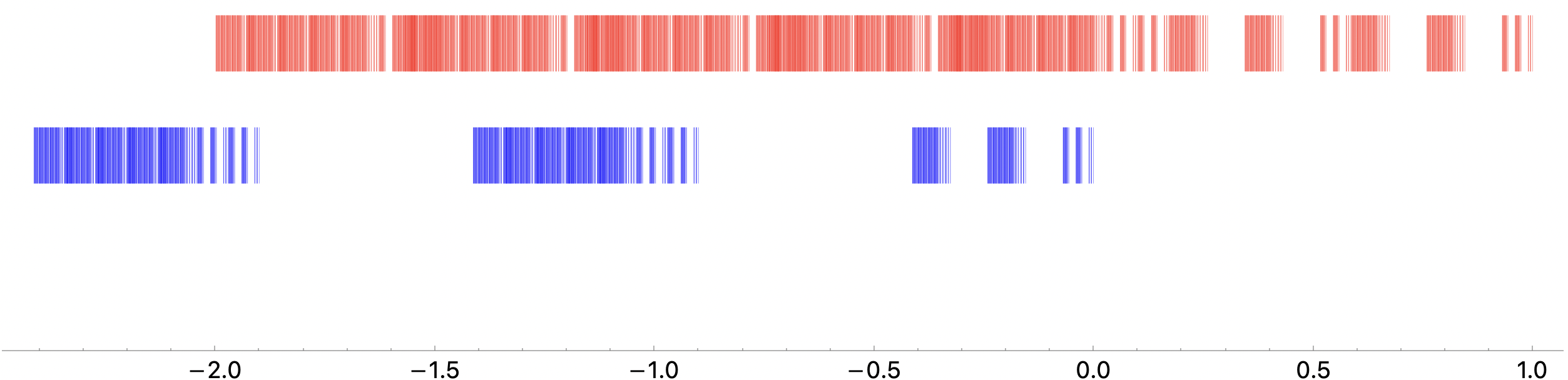
The fixed point of this contractive IFS, as $\lambda^{\star}<1$, is a Rauzy fractal; see Figure 2. By Proposition 2.5, these windows define regular model sets, and so does their union.

There are several ways to determine the Hausdorff dimension of the boundary of the window. One method, laborious but allowing a complete reconstruction of the window, involves the graph iterated function system of the window; see [10, 36]. Here, we use the overlap algorithm from [3, 8, 38], based on the discrepancy matrix; this is applicable to more complex tilings, but we need only consider our one-dimensional case. Consider two overlaid copies of the SSM tiling, one being a copy shifted by an element of the return module. We say a pair of tiles, one from each copy, form an overlap if the intersection of their supports has a non-empty interior. We can then consider the overlap itself as a tile determined by the support, the type of tiles from which it comes, and the offset of the two tiles. If the pair of tiles have the same type and position, we call it a coincidence overlap; otherwise, it is referred to as a discrepancy overlap. Therefore, from the original substitution, we can define another substitution on the overlaps; the corresponding substitution matrix is called the discrepancy matrix.

The Hausdorff dimension of the boundary $\partial W$ is then given [8, Prop. 6.1] by

$$\dim_{\mathrm{H}}(\partial W)\,=\,\overline{\dim}_{\mathrm{H}}(\partial W)\,=\,\frac{\,\log(\gamma)}{\log(\lambda_{\mathrm{PF}})}\hskip 0.5pt,$$

where $\overline{\dim}_{\mathrm{H}}(\partial W)$ is the maximum of $\overline{\dim}_{\mathrm{H}}(\partial W_{a,b}\hskip 0.5pt)$, $\lambda_{\mathrm{PF}}$ is the PF eigenvalue of the substitution matrix, and $\gamma$ is the spectral radius of the discrepancy matrix. The first equality holds because $\varLambda_{a}$ and $\varLambda_{b}$ are MLD to $\varLambda$, see [10] for details, thus the Hausdorff dimension of $\partial W_{a}$, $\partial W_{b}$, and $\partial W$ must be equal [13, Rem. 7.6]. Implementing this algorithm, an elementary calculation leads to the discrepancy matrix

$$M_{\text{dc}}\,=\,\begin{pmatrix}1&0&0&0&1&1&0\\ 1&0&0&0&0&0&0\\ 1&0&0&0&0&0&0\\ 1&0&0&0&0&0&0\\ 0&1&0&0&0&0&0\\ 0&0&1&0&0&1&1\\ 0&0&1&0&1&1&0\end{pmatrix}$$

with characteristic polynomial $\det(M_{\text{dc}}-x\mathbbm{1})=-x^{4}(x^{3}-2\hskip 0.5ptx^{2}-1)$. The spectral radius of $M_{\text{dc}}$ thus has a value of approximately $2.205{\hskip 0.5pt}57$, giving

$$\dim_{\mathrm{H}}(\partial W)\,=\,\frac{\,\log(\gamma)}{\log(\lambda_{\mathrm{PF}})}\,\approx\,0.897{\hskip 0.5pt}45\hskip 0.5pt.$$

Obviously, computing the covariogram of this window according to Definition 2.1 looks difficult if not impossible. To overcome this problem, we now introduce the renormalisation procedure. For the pair correlations $\nu_{\alpha\beta}$, where $\alpha,\beta\in\{a,b\}$, we have $\nu_{\alpha\beta}(z)=0$ for any $z\notin\varLambda_{\beta}-\varLambda_{\alpha}$ and $\nu_{\alpha\beta}(0)=0$ for $\alpha\neq\beta$. Moreover, the right PF eigenvector of (3.1) gives $\nu_{aa}(0)=\lambda^{-1}=\lambda-2$ and $\nu_{bb}(0)~=~\lambda^{-1}~\sqrt{2}~=~3-\lambda$. We also have the symmetry relation $\nu_{\alpha\beta}(-z)=\nu_{\beta\alpha}(z)$, and the summatory relationship

$$\nu(z)\,=\,\nu_{aa}(z)\,+\,\nu_{ab}(z)\,+\,\nu_{ba}(z)\,+\,\nu_{bb}(z)$$

from Proposition 2.2(vi).

With the symmetry relations and inflation structure, we can determine the renormalisation relations of $\nu_{\alpha\beta}$ as a special case of Proposition 2.7; see [26] for worked examples.

$z$	$0$	$1$	$2$	$3$	$\lambda-1$	$\lambda$	$2\lambda-2$	$\lambda+1$
$\nu_{aa}(z)$	$\lambda-2$	$0$	$0$	$0$	$\frac{3\,\lambda-7}{2}$	$\frac{3\hskip 0.5pt\lambda-7}{2}$	$0$	$\frac{17-7\,\lambda}{2}$
$\nu_{ab}(z)$	$0$	$0$	$0$	$0$	$\frac{3-\lambda}{2}$	$5-2\,\lambda$	$\frac{3\,\lambda-7}{2}$	$\frac{3\,\lambda-7}{2}$
$\nu_{ba}(z)$	$0$	$\frac{3-\lambda}{2}$	$5-2\,\lambda$	$\frac{3\,\lambda-7}{2}$	$0$	$\frac{3\,\lambda-7}{2}$	$0$	$5-2\,\lambda$
$\nu_{bb}(z)$	$3-\lambda$	$\frac{3-\lambda}{2}$	$\frac{3\,\lambda-7}{2}$	$0$	$0$	$5-2\,\lambda$	$0$	$5-2\,\lambda$

Table 1. The self-consistent part of the renormalisation equations for the SSM inflation tiling. Impossible distances (whose pair correlations evaluate to $0$ due to the tile geometry) are omitted. The column with $z=0$ contains the relative tile frequencies, as given by the right PF eigenvector of $M_{\varrho}$.

Theorem 3.1.

The pair correlations $\nu_{\alpha\beta}$ with $\alpha,\beta\in\{a,b\}$ of the SSM tiling satisfy the exact renormalisation relations

$$\lambda\nu_{aa}(z)\, =\,\nu_{aa}\Bigl(\frac{\raisebox{-2.0pt}{$z$}}{\raisebox{0.5pt}{$\lambda$}}\Bigr)\,+\,\nu_{ab}\Bigl(\frac{\raisebox{-2.0pt}{$z+2$}}{\raisebox{0.5pt}{$\lambda$}}\Bigr)\,+\,\nu_{ba}\Bigl(\frac{\raisebox{-2.0pt}{$z-2$}}{\raisebox{0.5pt}{$\lambda$}}\Bigr)\,+\,\nu_{bb}\Bigl(\frac{\raisebox{-2.0pt}{$z$}}{\raisebox{0.5pt}{$\lambda$}}\Bigr),$$

$$\lambda\nu_{ab}(z)\, =\,\nu_{aa}\Bigl(\frac{\raisebox{-2.0pt}{$z+2$}}{\raisebox{0.5pt}{$\lambda$}}\Bigr)\,+\,\nu_{aa}\Bigl(\frac{\raisebox{-2.0pt}{$z+1$}}{\raisebox{0.5pt}{$\lambda$}}\Bigr)\,+\,\nu_{ab}\Bigl(\frac{\raisebox{-2.0pt}{$z+3-\lambda$}}{\raisebox{0.5pt}{$\lambda$}}\Bigr)\,+\,\nu_{ba}\Bigl(\frac{\raisebox{-2.0pt}{$z$}}{\raisebox{0.5pt}{$\lambda$}}\Bigr)$$

$$\phantom{==}\,+\,\nu_{ba}\Bigl(\frac{\raisebox{-2.0pt}{$z-1$}}{\raisebox{0.5pt}{$\lambda$}}\Bigr)\,+\,\nu_{bb}\Bigl(\frac{\raisebox{-2.0pt}{$z+1-\lambda$}}{\raisebox{0.5pt}{$\lambda$}}\Bigr),$$

$$\lambda\nu_{ba}(z)\, =\,\nu_{aa}\Bigl(\frac{\raisebox{-2.0pt}{$z-2$}}{\raisebox{0.5pt}{$\lambda$}}\Bigr)\,+\,\nu_{aa}\Bigl(\frac{\raisebox{-2.0pt}{$z-1$}}{\raisebox{0.5pt}{$\lambda$}}\Bigr)\,+\,\nu_{ab}\Bigl(\frac{\raisebox{-2.0pt}{$z+1$}}{\raisebox{0.5pt}{$\lambda$}}\Bigr)\,+\,\nu_{ab}\Bigl(\frac{\raisebox{-2.0pt}{$z$}}{\raisebox{0.5pt}{$\lambda$}}\Bigr)$$

$$\phantom{==}\,+\,\nu_{ba}\Bigl(\frac{\raisebox{-2.0pt}{$z+\lambda-3$}}{\raisebox{0.5pt}{$\lambda$}}\Bigr)\,+\,\nu_{bb}\Bigl(\frac{\raisebox{-2.0pt}{$z-1+\lambda$}}{\raisebox{0.5pt}{$\lambda$}}\Bigr),$$

$$\lambda\nu_{bb}(z)\, =\,2\nu_{aa}\Bigl(\frac{\raisebox{-2.0pt}{$z$}}{\raisebox{0.5pt}{$\lambda$}}\Bigr)\,+\,\nu_{aa}\Bigl(\frac{\raisebox{-2.0pt}{$z+1$}}{\raisebox{0.5pt}{$\lambda$}}\Bigr)\,+\,\nu_{aa}\Bigl(\frac{\raisebox{-2.0pt}{$z-1$}}{\raisebox{0.5pt}{$\lambda$}}\Bigr)\,+\,\nu_{ab}\Bigl(\frac{\raisebox{-2.0pt}{$z+1-\lambda$}}{\raisebox{0.5pt}{$\lambda$}}\Bigr)$$

$$\phantom{==}\,+\,\nu_{ab}\Bigl(\frac{\raisebox{-2.0pt}{$z+2-\lambda$}}{\raisebox{0.5pt}{$\lambda$}}\Bigr)\,+\,\nu_{ba}\Bigl(\frac{\raisebox{-2.0pt}{$z+\lambda-2$}}{\raisebox{0.5pt}{$\lambda$}}\Bigr)\,+\,\nu_{ba}\Bigl(\frac{\raisebox{-2.0pt}{$z-1+\lambda$}}{\raisebox{0.5pt}{$\lambda$}}\Bigr)\,+\,\nu_{bb}\Bigl(\frac{\raisebox{-2.0pt}{$z+\lambda$}}{\raisebox{0.5pt}{$\lambda$}}\Bigr),$$

with $z\in\mathbb{Z}\hskip 0.5pt[\sqrt{2}\,]$, $\lambda=1+\sqrt{2}$, and $\nu_{\alpha\beta}(z)=0$ for $z\notin\varLambda_{\beta}-\varLambda_{\alpha}$. ∎

This is an infinite set of linear equations. However, via the inflation structure, all arguments with $|z|>\lambda+1$ are recursively determined from the self-consistent part of the equations. As this will be used later, we include the derivation. For a similar example, where the inflation factor is non-Pisot, we refer the reader to [6]. We remark that renormalisation does not need local recognisability, see [9], but it makes the process easier.

Figure 3. Representation of the window covariograms of the SSM system. The red function is $g_{aa}$, $g_{bb}$ is blue, $g_{ab}$ is black, $g_{ba}$ is grey, and the covariogram $g$ of the total window is pink. The plot of $g$ consists of $35{\hskip 0.5pt\hskip 0.5pt}323$ points; we also include a closer view of a small section to illustrate the irregular behaviour.

Proposition 3.2.

Consider the renormalisation relations of Theorem 3.1 with the symmetry and vanishing conditions, and the arguments restricted to $z\in\varLambda-\varLambda$ with $|z|\leqslant\lambda+1$. This is a finite, closed set of equations with a one-dimensional solution space. In particular, once $\nu_{aa}(0)$ is given, the solution is unique.

Proof.

By symmetry, we need only to look at $z\geqslant 0$, and when $z\leqslant\lambda+1$, no argument on the right-hand side of the identities in Theorem 3.1 exceeds $\lambda+1$. We thus consider

$$\varLambda-\varLambda\cap[0,\lambda+1]\,=\,\{0\hskip 0.5pt,\,1\hskip 0.5pt,\,2\hskip 0.5pt,\,3\hskip 0.5pt,\,\lambda-1\hskip 0.5pt,\,\lambda\hskip 0.5pt,\,2\lambda-2\hskip 0.5pt,\,\lambda+1\}\hskip 0.5pt,$$

which gives the first claim. We have omitted any values prohibited by the tile geometry, as all pair correlations would then be zero. The values for $z=0$ follow from the PF eigenvector, and the fact that a tile can only have one type. The geometry of the tiles implies the other occurrences of $0$ in Table 1; however, these can also be checked using the relations from Theorem 3.1 and the vanishing conditions. Note that $\lambda^{-1}=\lambda-2$, $\lambda^{2}=1+2\lambda$, and $\lambda^{\star}=-\lambda^{-1}$. Using these relations, we can easily solve the resulting finite set of equations by hand, the details of which are omitted. In particular, $\nu_{aa}(0)$ is not fixed by the relations, and all other values can be written in terms of $\nu_{aa}(0)$; thus, the solution space is indeed one-dimensional.

Uniqueness follows from $\nu_{aa}(0)+\nu_{bb}(0)=1$, with the values listed in Table 1, where the interpretation of $\nu_{aa}(0)$ and $\nu_{bb}(0)$ as the relative tile frequencies was used. ∎

A similar proof was given in [26], to which we refer the reader for further details and examples. Via the correspondence between the equations from Propositions 2.7 and 2.8, this also gives us the renormalisation approach to the covariogram functions $g_{\alpha\beta}$. We can now plot the covariograms using the recursive structure of the equations, with the self-consistent part serving as initial values. The result is shown in Figure 3. Despite their appearance, by Proposition 2.2, each function is continuous and also bounded above by a tent function. Moreover, as mentioned in Remark 2.6, Figure 3 is an acceptable illustration of the covariogram as we know its exact value at a dense and uniformly distributed set of points, in combination with the continuity of the function.

Figure 4. Illustration of the windows for the substitution $\sigma$; $W_{a}$ is red (top) and $W_{b}$ is blue (bottom). As before, the windows are one-dimensional, but we assign some fixed arbitrary height to the points for illustration. Furthermore, by Proposition 2.5, the windows are measure-theoretically disjoint, but we are limited by the resolution of the plot and the large Hausdorff dimension of the window boundaries.

3.2. A more complex example

Next, we construct another window system, with the same CPS, whose boundaries exhibit even stronger fractal behaviour than that of the SSM system. Consider the substitution

$$\sigma\,:\,\begin{cases}a\mapsto aaaaabb\hskip 0.5pt,\\ \hskip 0.5ptb\hskip 0.5pt\mapsto baa\hskip 0.5pt,\end{cases}$$

with corresponding substitution matrix $M_{\sigma}=\big(\begin{smallmatrix}5&2\\ 2&1\end{smallmatrix}\big)$ and PF eigenvalue

$$\lambda_{\mathrm{PF}}=\lambda^{2}=2\lambda+1=3+2\sqrt{2}\hskip 0.5pt.$$

The left and (statistically normalised) right PF eigenvectors are given by

(3.4) $$w_{\ell}\,=\,(\lambda,1)\quad\text{and}\quad w_{r}\,=\,\Bigl(\frac{\raisebox{-2.0pt}{$\lambda-1$}}{\raisebox{0.5pt}{$2$}},\,\frac{\raisebox{-2.0pt}{$3-\lambda$}}{\raisebox{0.5pt}{$2$}}\Bigr)^{\!\top}.$$

This substitution produces a tiling of $\mathbb{R}\hskip 0.5pt$ in an analogous way as before. To determine the window, we go through the same procedure as in the previous section. The relations for the sets $\varLambda_{a}$ and $\varLambda_{b}$ are given by

$$\begin{split}\varLambda_{a}\,&=\,\lambda^{2}\varLambda_{a}\;\dot{\cup}\;\big(\lambda^{2}\varLambda_{a}\,{{+}}\,\lambda\big)\;\dot{\cup}\;\big(\lambda^{2}\varLambda_{a}\,{{+}}\,2\lambda\big)\,\,\dot{\cup}\,\big(\lambda^{2}\varLambda_{a}\,{{+}}\,3\lambda\big)\\[3.0pt] &\qquad\quad\quad\hskip-0.5pt\dot{\cup}\,\big(\lambda^{2}\varLambda_{a}\,{{+}}\,4\lambda\big)\;\dot{\cup}\;\big(\lambda^{2}\varLambda_{b}\,{{+}}\,1\big)\;\dot{\cup}\;\big(\lambda^{2}\varLambda_{b}\,{{+}}\,\lambda\,{{+}}\,1\big),\\[5.0pt] \varLambda_{b}\,&=\,\big(\lambda^{2}\varLambda_{a}\,{{+}}\,5\lambda\big)\;\dot{\cup}\;\big(\lambda^{2}\varLambda_{a}\,{{+}}\,5\lambda\,{{+}}\,1\big)\;\dot{\cup}\;\big(\lambda^{2}\varLambda_{b}\big).\end{split}$$

Again, taking $W_{a,b}:=\overline{\varLambda^{\star}_{a,b}}$ gives the following internal space IFS,

$$\begin{split}W_{a}\,&=\,\lambda^{-2}W_{a}\,\cup\,\big(\lambda^{-2}W_{a}\,{{-}}\,\lambda^{-1}\big)\,\cup\,\big(\lambda^{-2}W_{a}\,{{-}}\,2\lambda^{-1}\big)\,\cup\,\big(\lambda^{-2}W_{a}\,{{-}}\,3\lambda^{-1}\big)\\[3.0pt] &\qquad\quad\quad\;\;\,\cup\,\big(\lambda^{-2}W_{a}\,{{-}}\,4\,\lambda^{-1}\big)\,\cup\,\big(\lambda^{-2}W_{b}\,{{+}}\,1\big)\,\,\cup\,\big(\lambda^{-2}W_{b}\,{{+}}\,1\,{{-}}\,\lambda^{-1}\big),\\[5.0pt] W_{b}\,&=\,\big(\lambda^{-2}W_{a}\,{{-}}\,5\lambda^{-1}\big)\,\cup\,\big(\lambda^{-2}W_{a}\,{{+}}\,1\,{{-}}\,5\lambda^{-1}\big)\,\cup\,\big(\lambda^{-2}W_{b}\big).\end{split}$$

The fixed point of this contractive IFS is again the window system, illustrated in Figure 4. Via the overlap algorithm, the dimension of the fractal boundary is determined to be

$$\dim_{\mathrm{H}}(\partial W)\,=\,\frac{\,\log(\gamma)}{\log(\lambda_{\mathrm{PF}})}\,\approx\,0.966{\hskip 0.5pt}4739\hskip 0.5pt,$$

where $\gamma\approx 5.493{\hskip 0.5pt}959$ is the largest root of $x^{3}-7x^{2}+7x+7$, the characteristic polynomial of the discrepancy matrix. The renormalisation relations are as follows.

$z$	$0$	$1$	$2$	$3$	$\lambda$	$\lambda+1$	$\lambda+2$	$\lambda+3$	$2\,\lambda$	$2\,\lambda+1$
$\nu_{aa}(z)$	$\frac{\lambda-1}{2}$	$0$	$0$	$0$	$\frac{3\,\lambda-5}{4}$	$\frac{17-7\,\lambda}{4}$	$\frac{13\,\lambda-31}{4}$	$\frac{17-7\,\lambda}{4}$	$\lambda-2$	$17-7\,\lambda$
$\nu_{ab}(z)$	$0$	$0$	$0$	$0$	$\frac{3-\lambda}{4}$	$\frac{3\,\lambda-7}{2}$	$\frac{17-7\,\lambda}{4}$	$0$	$\frac{3-\lambda}{4}$	$\frac{3\,\lambda-7}{2}$
$\nu_{ba}(z)$	$0$	$\frac{3-\lambda}{4}$	$\frac{3\,\lambda-7}{2}$	$\frac{17-7\,\lambda}{4}$	$0$	$\frac{3\lambda-7}{4}$	$\frac{3\,\lambda-7}{2}$	$\frac{17-7\,\lambda}{4}$	$0$	$\frac{3\,\lambda-7}{2}$
$\nu_{bb}(z)$	$\frac{3-\lambda}{2}$	$\frac{3-\lambda}{4}$	$\frac{17-7\,\lambda}{4}$	$0$	$0$	$0$	$0$	$0$	$0$	$\frac{17-7\,\lambda}{2}$

Table 2. The self-consistent part of the renormalisation equations for the tiling arising from $\sigma$, with the natural tile lengths given by the left PF eigenvector. Distances which are not possible, i.e., ones for which all pair correlations evaluate to zero due to the tile geometry, are omitted. The column corresponding to $z=0$ contains the relative tile frequencies, as given by the (statistically normalised) right PF eigenvector of $M_{\sigma}$.

Theorem 3.3.

The pair correlations $\nu_{\alpha\beta}$ with $\alpha,\beta\in\{a,b\}$ of the tiling induced by $\sigma$ satisfy the exact renormalisation relations

$$\lambda^{2}\nu_{aa}(z)\, =\,5\nu_{aa}\Bigl(\frac{\raisebox{-2.0pt}{$z$}}{\raisebox{0.5pt}{$\lambda^{2}$}}\Bigr)+4\nu_{aa}\Bigl(\frac{\raisebox{-2.0pt}{$z-\lambda$}}{\raisebox{0.5pt}{$\lambda^{2}$}}\Bigr)+4\nu_{aa}\Bigl(\frac{\raisebox{-2.0pt}{$z+\lambda$}}{\raisebox{0.5pt}{$\lambda^{2}$}}\Bigr)+3\nu_{aa}\Bigl(\frac{\raisebox{-2.0pt}{$z-2\,\lambda$}}{\raisebox{0.5pt}{$\lambda^{2}$}}\Bigr)+\nu_{bb}\Bigl(\frac{\raisebox{-2.0pt}{$z+\lambda$}}{\raisebox{0.5pt}{$\lambda^{2}$}}\Bigr)$$

$$\phantom{==}+3\nu_{aa}\Bigl(\frac{\raisebox{-2.0pt}{$z+2\lambda$}}{\raisebox{0.5pt}{$\lambda^{2}$}}\Bigr)+2\nu_{aa}\Bigl(\frac{\raisebox{-2.0pt}{$z-3\,\lambda$}}{\raisebox{0.5pt}{$\lambda^{2}$}}\Bigr)+2\nu_{aa}\Bigl(\frac{\raisebox{-2.0pt}{$z+3\,\lambda$}}{\raisebox{0.5pt}{$\lambda^{2}$}}\Bigr)+\nu_{aa}\Bigl(\frac{\raisebox{-2.0pt}{$z-4\,\lambda$}}{\raisebox{0.5pt}{$\lambda^{2}$}}\Bigr)$$

$$\phantom{==}+\nu_{aa}\Bigl(\frac{\raisebox{-2.0pt}{$z+4\,\lambda$}}{\raisebox{0.5pt}{$\lambda^{2}$}}\Bigr)+2\nu_{ab}\Bigl(\frac{\raisebox{-2.0pt}{$z-1$}}{\raisebox{0.5pt}{$\lambda^{2}$}}\Bigr)+2\nu_{ba}\Bigl(\frac{\raisebox{-2.0pt}{$z+1$}}{\raisebox{0.5pt}{$\lambda^{2}$}}\Bigr)+\nu_{ab}\Bigl(\frac{\raisebox{-2.0pt}{$z-\lambda-1$}}{\raisebox{0.5pt}{$\lambda^{2}$}}\Bigr)$$

$$\phantom{==}+\nu_{ba}\Bigl(\frac{\raisebox{-2.0pt}{$z+\lambda+1$}}{\raisebox{0.5pt}{$\lambda^{2}$}}\Bigr)+\nu_{ab}\Bigl(\frac{\raisebox{-2.0pt}{$z+4\,\lambda-1$}}{\raisebox{0.5pt}{$\lambda^{2}$}}\Bigr)+\nu_{ba}\Bigl(\frac{\raisebox{-2.0pt}{$z-4\,\lambda+1$}}{\raisebox{0.5pt}{$\lambda^{2}$}}\Bigr)+\nu_{bb}\Bigl(\frac{\raisebox{-2.0pt}{$z-\lambda$}}{\raisebox{0.5pt}{$\lambda^{2}$}}\Bigr)$$

$$\phantom{==}+2\nu_{ab}\Bigl(\frac{\raisebox{-2.0pt}{$z+\lambda-1$}}{\raisebox{0.5pt}{$\lambda^{2}$}}\Bigr)+2\nu_{ba}\Bigl(\frac{\raisebox{-2.0pt}{$z-\lambda+1$}}{\raisebox{0.5pt}{$\lambda^{2}$}}\Bigr)+2\nu_{ab}\Bigl(\frac{\raisebox{-2.0pt}{$z+2\lambda-1$}}{\raisebox{0.5pt}{$\lambda^{2}$}}\Bigr)+2\nu_{bb}\Bigl(\frac{\raisebox{-2.0pt}{$z$}}{\raisebox{0.5pt}{$\lambda^{2}$}}\Bigr)$$

$$\phantom{==}+2\nu_{ba}\Bigl(\frac{\raisebox{-2.0pt}{$z-2\,\lambda+1$}}{\raisebox{0.5pt}{$\lambda^{2}$}}\Bigr)+2\nu_{ab}\Bigl(\frac{\raisebox{-2.0pt}{$z+3\,\lambda-1$}}{\raisebox{0.5pt}{$\lambda^{2}$}}\Bigr)+2\nu_{ba}\Bigl(\frac{\raisebox{-2.0pt}{$z-3\,\lambda+1$}}{\raisebox{0.5pt}{$\lambda^{2}$}}\Bigr)\hskip 0.5pt,$$

$$\lambda^{2}\nu_{bb}(z)\, =\,2\nu_{aa}\Bigl(\frac{\raisebox{-2.0pt}{$z$}}{\raisebox{0.5pt}{$\lambda^{2}$}}\Bigr)+\nu_{aa}\Bigl(\frac{\raisebox{-2.0pt}{$z-1$}}{\raisebox{0.5pt}{$\lambda^{2}$}}\Bigr)+\nu_{ab}\Bigl(\frac{\raisebox{-2.0pt}{$z+5\,\lambda$}}{\raisebox{0.5pt}{$\lambda^{2}$}}\Bigr)+\nu_{aa}\Bigl(\frac{\raisebox{-2.0pt}{$z+1$}}{\raisebox{0.5pt}{$\lambda^{2}$}}\Bigr)$$

$$\phantom{==}+\nu_{ab}\Bigl(\frac{\raisebox{-2.0pt}{$z+5\,\lambda+1$}}{\raisebox{0.5pt}{$\lambda^{2}$}}\Bigr)+\nu_{ba}\Bigl(\frac{\raisebox{-2.0pt}{$z-5\,\lambda$}}{\raisebox{0.5pt}{$\lambda^{2}$}}\Bigr)+\nu_{ba}\Bigl(\frac{\raisebox{-2.0pt}{$z-5\,\lambda-1$}}{\raisebox{0.5pt}{$\lambda^{2}$}}\Bigr)+\nu_{bb}\Bigl(\frac{\raisebox{-2.0pt}{$z$}}{\raisebox{0.5pt}{$\lambda^{2}$}}\Bigr),$$

$$\lambda^{2}\nu_{ab}(z)\, =\,\nu_{aa}\Bigl(\frac{\raisebox{-2.0pt}{$z-5\lambda$}}{\raisebox{0.5pt}{$\lambda^{2}$}}\Bigr)+\nu_{aa}\Bigl(\frac{\raisebox{-2.0pt}{$z-5\lambda-1$}}{\raisebox{0.5pt}{$\lambda^{2}$}}\Bigr)+\nu_{ab}\Bigl(\frac{\raisebox{-2.0pt}{$z$}}{\raisebox{0.5pt}{$\lambda^{2}$}}\Bigr)+\nu_{aa}\Bigl(\frac{\raisebox{-2.0pt}{$z-4\lambda$}}{\raisebox{0.5pt}{$\lambda^{2}$}}\Bigr)+\nu_{ba}\Bigl(\frac{\raisebox{-2.0pt}{$z-4\lambda$}}{\raisebox{0.5pt}{$\lambda^{2}$}}\Bigr)$$

$$\phantom{==}+\nu_{aa}\Bigl(\frac{\raisebox{-2.0pt}{$z-4\lambda-1$}}{\raisebox{0.5pt}{$\lambda^{2}$}}\Bigr)+\nu_{ab}\Bigl(\frac{\raisebox{-2.0pt}{$z+\lambda$}}{\raisebox{0.5pt}{$\lambda^{2}$}}\Bigr)+\nu_{aa}\Bigl(\frac{\raisebox{-2.0pt}{$z-3\lambda$}}{\raisebox{0.5pt}{$\lambda^{2}$}}\Bigr)+\nu_{aa}\Bigl(\frac{\raisebox{-2.0pt}{$z-3\lambda-1$}}{\raisebox{0.5pt}{$\lambda^{2}$}}\Bigr)$$

$$\phantom{==}+\nu_{ab}\Bigl(\frac{\raisebox{-2.0pt}{$z+2\lambda$}}{\raisebox{0.5pt}{$\lambda^{2}$}}\Bigr)+\nu_{aa}\Bigl(\frac{\raisebox{-2.0pt}{$z-2\lambda$}}{\raisebox{0.5pt}{$\lambda^{2}$}}\Bigr)+\nu_{aa}\Bigl(\frac{\raisebox{-2.0pt}{$z-2\lambda-1$}}{\raisebox{0.5pt}{$\lambda^{2}$}}\Bigr)+\nu_{ab}\Bigl(\frac{\raisebox{-2.0pt}{$z+3\lambda$}}{\raisebox{0.5pt}{$\lambda^{2}$}}\Bigr)$$

$$\phantom{==}+\nu_{aa}\Bigl(\frac{\raisebox{-2.0pt}{$z-\lambda$}}{\raisebox{0.5pt}{$\lambda^{2}$}}\Bigr)+\nu_{aa}\Bigl(\frac{\raisebox{-2.0pt}{$z-\lambda-1$}}{\raisebox{0.5pt}{$\lambda^{2}$}}\Bigr)+\nu_{ab}\Bigl(\frac{\raisebox{-2.0pt}{$z+4\lambda$}}{\raisebox{0.5pt}{$\lambda^{2}$}}\Bigr)+\nu_{ba}\Bigl(\frac{\raisebox{-2.0pt}{$z+1-5\lambda$}}{\raisebox{0.5pt}{$\lambda^{2}$}}\Bigr)$$

$$\phantom{==}+\nu_{ba}\Bigl(\frac{\raisebox{-2.0pt}{$z-5\lambda$}}{\raisebox{0.5pt}{$\lambda^{2}$}}\Bigr)+\nu_{bb}\Bigl(\frac{\raisebox{-2.0pt}{$z+1$}}{\raisebox{0.5pt}{$\lambda^{2}$}}\Bigr)+\nu_{ba}\Bigl(\frac{\raisebox{-2.0pt}{$z+1-4\lambda$}}{\raisebox{0.5pt}{$\lambda^{2}$}}\Bigr)+\nu_{bb}\Bigl(\frac{\raisebox{-2.0pt}{$z+\lambda+1$}}{\raisebox{0.5pt}{$\lambda^{2}$}}\Bigr),$$

together with $\nu_{ba}(z)=\nu_{ab}(-z)$, $z\in\mathbb{Z}\hskip 0.5pt[\sqrt{2}\,]$, $\lambda=1+\sqrt{2}$, and $\nu_{\alpha\beta}(z)=0$ for $z\notin\varLambda_{\beta}-\varLambda_{\alpha}$. ∎

The self-consistent part of the relations is listed in Table 2. As the calculations are analogous to Proposition 3.2, we omit a proof.

Figure 5. Point plot, with $188{\hskip 0.5pt\hskip 0.5pt}214$ points, of the covariogram of the window of Figure 4. Here, the splitting behaviour is highlighted; the distances involving an even number of $b$’s are blue, and those with an odd number are red.

Corollary 3.4.

Consider the renormalisation relations of Theorem 3.3 with the symmetry and vanishing conditions, and the arguments restricted to $z\in\varLambda-\varLambda$ with $|z|\leqslant 2\,\lambda+1$. This is a finite, closed set of equations with a one-dimensional solution space. In particular, once $\nu_{aa}(0)$ is given, the solution is unique. ∎

The covariogram can now be computed as before, and is shown in Figures 5 and 6. We remark again that this is indeed a continuous function, despite its highly discontinuous appearance. To our knowledge, this is the first example of such a covariogram having a ‘splitting’ behaviour. One can do the following as a consistency check for the continuity. Take a large patch of the tiling, approximately $500{\hskip 0.5pt\hskip 0.5pt}000$ tiles, and construct the set of tile coordinates. The Minkowski difference of this set is then taken with itself; with the above number of tiles, it should produce approximately five million distinct distances. To efficiently run this set of distances through the relations from Theorem 3.3, one can implement a ‘valid distance’ test; this checks whether the integer coordinates of $z=a\hskip 0.5pt\lambda+b$ have the same parity (or are zero) and whether $z^{\star}$ lies in a bounded region of internal space. The distance $z$ is then passed to the relations only if both requirements are met. Additionally, running the relations in parallel significantly improves computation time.

Figure 6. Point plot, derived from $4{\hskip 0.5pt\hskip 0.5pt}826{\hskip 0.5pt\hskip 0.5pt}361$ points, of the covariogram of the window of Fig. 4. The closer view illustrates the slow convergence and complex behaviour of the function.

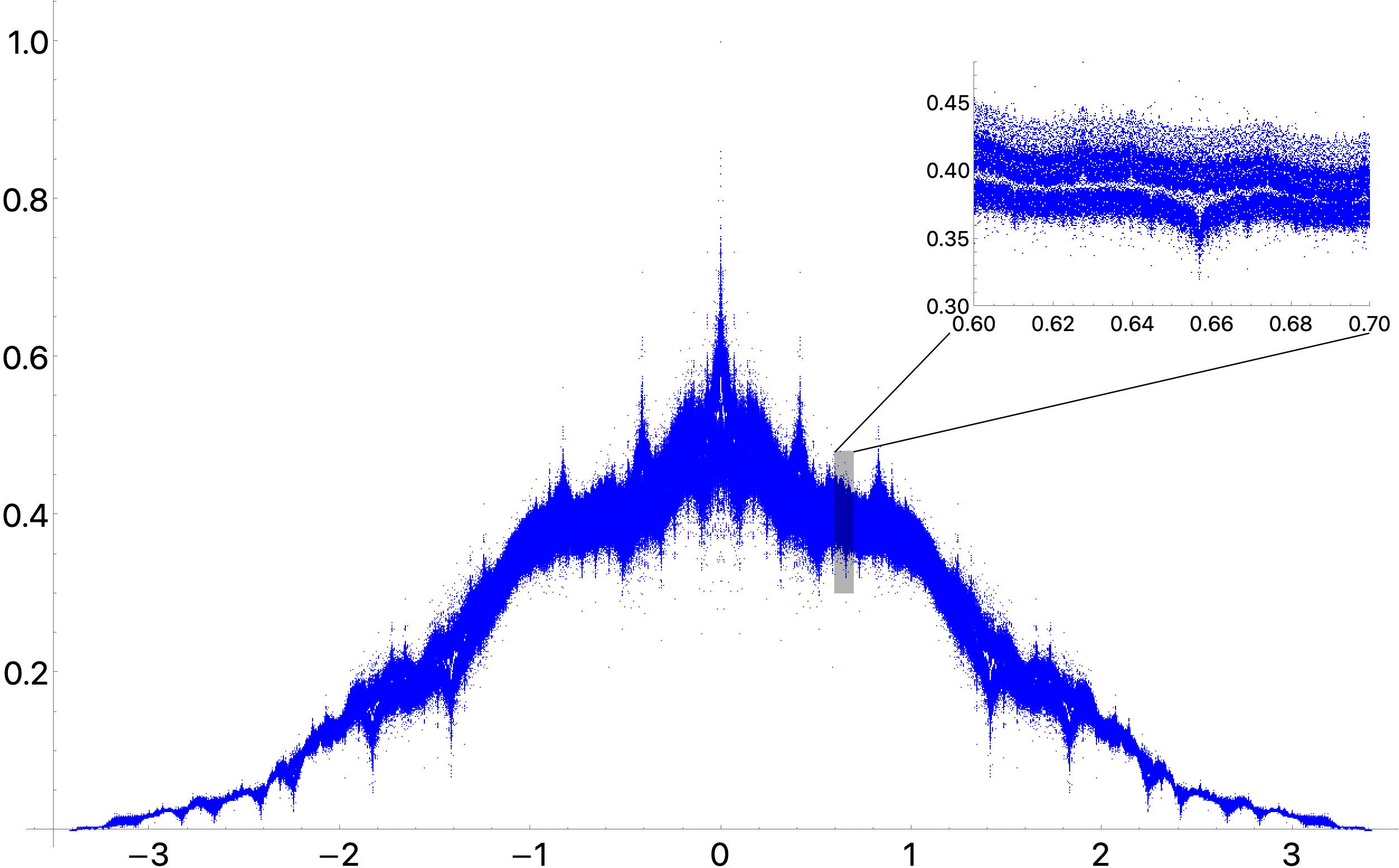
With these large samples, one sees that the gap will close, albeit incredibly slowly; Figure 6 illustrates this behaviour. We emphasise again, as in Remark 2.6 and in the previous example, that this is a valid approximation of the continuous function as we are sampling from a dense and uniformly distributed subset of the support. The upper and lower branches of the split can be identified as those distances which contain, respectively, an even and odd number of $b$’s. This behaviour is thus a consequence of the combinatorics of the substitution and not triggered by the high boundary dimension of the window, as one might first guess. This is well worth further examination, but is far beyond the scope of this brief note. Also, with regard to the original question of a natural counterpart to the theta series of periodic point sets, the complex behaviour of the covariograms will also call for a renewed, and perhaps conceptually different, approach to aperiodic theta series.

Our above analysis was based on one-dimensional inflation tilings with an internal space that is also one-dimensional. It is an obvious task to extend both to higher dimensions. In a first step, one should consider unimodular inflation tilings with a ternary alphabet, thus giving Rauzy fractals in $\mathbb{R}\hskip 0.5pt^{2}$. First results on the Kolakoski sequence are presented in [26], and the same type of analysis can be done for the classic Tribonacci sequence. Computationally, both are significantly more involved yet of limited value because the windows are simply connected sets with a fractal boundary. The resulting covariograms still look well behaved and mainly smooth. More interesting would be the twisted Tribonacci sequence [5, 8], which leads to a disconnected window system that may be considered as an analogue of a Cantorval. More work is needed to explore the possibilities here.

References

- [1] C. Alfes, P. Kiefer and J. Mazáč, Measures, modular forms, and summation formulas of Poisson type, Commun. Math. Phys. 406 (2025), art. 137 (23 pp); arXiv:2405.15620.
- [2] S. Akiyama, M. Barge, V. Berthé, J-Y. Lee and A. Siegel, On the Pisot substitution conjecture, in: Mathematics of Aperiodic Order, eds. J. Kellendonk, D. Lenz and J. Savinien, Birkhäuser, Basel (2015), pp. 33–72.
- [3] S. Akiyama, and J-Y. Lee, Algorithm for determining pure pointedness of self-affine tilings, Adv. Math. 226 (2011), 2855–2883; arXiv:1003.2898.
- [4] P. Arnoux and E. Harriss, What is a Rauzy fractal, Notices Amer. Math. Soc. 61 (2014), 768–770.
- [5] P. Arnoux and S. Ito, Pisot Substitutions and Rauzy fractals, Bull. Belg. Math. Soc. 8 (2001), 181–207.
- [6] M. Baake, N. P. Frank, U. Grimm and E. A. Robinson, Geometric properties of a binary non-Pisot inflation and absence of absolutely continuous diffraction, Studia Math. 247 (2019), 109–154; arXiv:1706.03976.
- [7] M. Baake and F. Gähler, Pair correlations of aperiodic inflation rules via renormalisation: Some interesting examples, Topol. Appl. 205 (2016), 4–27; arXiv:1511.00885.
- [8] M. Baake, F. Gähler and P. Gohlke, Orbit separation dimension as complexity measure for primitive inflation tilings, Ergod. Th. Dynam. Syst. 45 (2025), 2992–3020; arXiv:2311.03541.
- [9] M. Baake, F. Gähler and N. Mañibo, Renormalisation of pair correlation measures for primitive inflation rules and absence of absolutely continuous diffraction, Commun. Math. Phys. 370 (2019), 591–635; arXiv:1805.09650.
- [10] M. Baake, A. Gorodetski and J. Mazáč, A naturally appearing family of Cantorvals, Lett. Math. Phys. 114 (2024), art. 101 (11 pp); arXiv:2401.05372.
-
[11]
M. Baake and U. Grimm,
A note on shelling,
Discr. Comput. Geom. 30 (2003), 573–589;
arXiv:math/0203025. - [12] M. Baake and U. Grimm, Homometric model sets and window covariograms, Z. Krist. 222 (2007), 54–58; arXiv:math/0610411.
- [13] M. Baake and U. Grimm, Aperiodic Order. Vol. 1: A Mathematical Invitation, Cambridge University Press, Cambridge (2013).
- [14] M. Baake and U. Grimm, Fourier transform of Rauzy fractals and point spectrum of 1D Pisot inflation tilings, Docum. Math. 25 (2020), 2303–2337; arXiv:1907.11012.
- [15] M. Baake and R. V. Moody, Self-similar measures for quasicrystals, in: Directions in Mathematical Quasicrystals, eds. M. Baake and R. V. Moody, CRM Monograph Series, vol. 13, AMS, Providence RI, 2000, pp. 1–42.
- [16] S. Balchin and D. Rust, Computations for symbolic substitutions, J. Int. Seq. 20 (2017), art. 17.4.1 (36pp); arXiv:1705.11130.
- [17] M. Barge, Pure discrete spectrum for a class of one-dimensional substitution tiling systems, Discr. Cont. Dynam. Syst. A 36 (2016), 1159–1173; arXiv:1403.7826.
- [18] M. Barge and J. Kwapisz, Geometric theory of of unimodular Pisot substitutions, Amer. J. Math. 128 (2006), 1219–1282.
- [19] V. Berthé, A. Siegel and J. Thuswaldner, Substitutions, Rauzy fractals and tilings, in: Combinatorics, Automata and Number Theory, ed. V. Berthé, Cambridge Univ. Press, Cambridge (2010), pp. 248–323.
- [20] G. Bianchi, The covariogram problem, in: Harmonic Analysis and Convexity, eds. A. Koldobsky and A. Volbergs, de Gruyter, Berlin (2023), pp. 37–82.
- [21] M. Björklund, T. Hartnick, Y. Karasik, Intersection spaces and multiple transverse recurrence, J. Anal. Math. 156 (2025), 97–150; arXiv:2108.09064.
- [22] J. H. Conway and N. J. A. Sloane, Sphere Packings, Lattices and Groups, 3rd ed., Springer, New York, (1999).
- [23] M. Hollander and B. Solomyak, Two-symbol Pisot substitutions have pure discrete spectrum, Ergod. Th. Dynam. Syst. 23 (2003), 533–540.
- [24] J. E. Hutchinson, Fractals and self-similarity, Indiana Univ. Math. J. 30 (1981), 713–747.
- [25] S. Ito and H. Rao, Atomic surfaces, tilings and coincidence I: irreducible case, Israel J. Math. 153 (2006), 129–155.
- [26] A. Klick, Averaged Shelling of Model Sets via Renormalisation, Master thesis, Univ. Bielefeld (2024).
- [27] H. Koch, Number Theory: Algebraic Numbers and Functions, Amer. Math. Soc., Providence, RI (2000).
- [28] L. Kuipers and H. Niederreiter, Uniform Distribution of Sequences, reprint, Dover, New York (2006).
[29]
N. Mañibo,
Lyapunov Exponents in the Spectral Theory of Primitive
Inflation Systems,
PhD thesis, Univ. Bielefeld (2019),
available electronically at urn:nbn:de:0070-pub-29359727. - [30] J. Mazáč, Fractal and Statistical Phenomena in Aperiodic Order, PhD thesis, Univ. Bielefeld (2025), available electronically at urn:nbn:de:0070-pub-30062996.
[31]
J. Mazáč,
Exact renormalisation for patch frequencies in inflation systems,
preprint (2025);
arXiv:2507.07753. - [32] Y. Meyer, Algebraic Numbers and Harmonic Analysis, North Holland, Amsterdam (1972).
- [33] R. V. Moody, Meyer sets and their duals, in: The Mathematics of Long-Range Aperiodic Order, ed. R. V. Moody, Kluwer, Dordrecht (1997), pp. 403–441.
- [34] R. V. Moody and A. Weiss, On shelling quasicrystals, J. Number Th. 47 (1994), 405–412.
- [35] A. Siegel and J. Thuswaldner, Topological Properties of Rauzy Fractals, Sociéte Mathématique de France, Paris (2009).
- [36] B. Sing, Pisot Substitutions and Beyond, PhD thesis, Univ. Bielefeld (2007), available electronically at urn:nbn:de:hbz:361-11555.
- [37] V. F. Sirvent and Y. Wang, Self-affine tiling via substitution dynamical systems and Rauzy fractals, Pacific J. Math. 206 (2002), 465–485.
- [38] B. Solomyak, Dynamics of self-similar tilings, Ergod. Th. Dynam. Syst. 17 (1997), 695–738, and Ergod. Th. Dynam. Syst. 19 (1999), 1685–1685 (erratum).