arXiv is now an independent nonprofit! Learn more
License: arXiv.org perpetual non-exclusive license
arXiv:2502.16819v2 [cs.LG] 12 Aug 2025

Fast, Accurate Manifold Denoising by
Tunneling Riemannian Optimization

Shiyu Wang Affiliation: Department of Electrical Engineering, Columbia University Affiliation: Data Science Institute, Columbia University Correspondence to: sw3601@columbia.edu    Mariam Avagyan Affiliation: Department of Electrical Engineering, Columbia University Affiliation: Data Science Institute, Columbia University    Yihan Shen Affiliation: Department of Computer Science, Columbia University Affiliation: Data Science Institute, Columbia University    Arnaud Lamy Affiliation: Department of Electrical Engineering, Columbia University Affiliation: Data Science Institute, Columbia University    Tingran Wang Affiliation: Department of Electrical Engineering, Columbia University Affiliation: Data Science Institute, Columbia University    Szabolcs Márka Affiliation: Department of Physics Affiliation: Data Science Institute, Columbia University Affiliation: Institute of Advanced Studies (iASK), Chernel utca 14, Kőszeg, 9730, Hungary    Zsuzsanna Márka Affiliation: Columbia Astrophysics Laboratory Affiliation: Data Science Institute, Columbia University    John Wright Affiliation: Department of Electrical Engineering, Columbia University Affiliation: Department of Applied Physics and Applied Mathematics, Columbia University Affiliation: Data Science Institute, Columbia University
Abstract

Learned denoisers play a fundamental role in various signal generation (e.g., diffusion models) and reconstruction (e.g., compressed sensing) architectures, whose success derives from their ability to leverage low-dimensional structure in data. Existing denoising methods, however, either rely on local approximations that require a linear scan of the entire dataset or treat denoising as generic function approximation problems, sacrificing efficiency and interpretability. We consider the problem of efficiently denoising a new noisy data point sampled from an unknown dd-dimensional manifold ℳ∈ℝD\mathcal{M}\in\mathbb{R}^{D}, using only noisy samples. This work proposes a framework for test-time efficient manifold denoising, by framing the concept of “learning-to-denoise” as “learning-to-optimize”. We have two technical innovations: (i) online learning methods which learn to optimize over the manifold of clean signals using only noisy data, effectively “growing” an optimizer one sample at a time. (ii) mixed-order methods which guarantee that the learned optimizers achieve global optimality, ensuring both efficiency and near-optimal denoising performance. We corroborate these claims with theoretical analyses of both the complexity and denoising performance of mixed-order traversal. Our experiments on scientific manifolds demonstrate significantly improved complexity-performance tradeoffs compared to nearest neighbor search, which underpins existing provable denoising approaches based on exhaustive search.

Keywords: 
Machine Learning, ICML

1 Introduction

Denoising is a core task in signal and image processing. Denoisers also play a fundamental role in state-of-the-art approaches to signal generation and reconstruction. Diffusion models generate intricate images from pure noise, via a sequence of denoising steps; learned compressed sensing methods reconstruct accurate medical and scientific images from incomplete, indirect measurements, again via a sequence of denoising steps. While these iterative procedures produce high-quality results, they are computationally costly: a sophisticated learned denoiser needs to be applied repeatedly to produce a single output. The test-time cost of denoising is a major bottleneck for both high-resolution image generation and real-time image reconstruction.

Accurate denoising is critical, because the denoiser encodes prior knowledge about the set of images of interest (natural, medical, scientific, etc.). These images reside near low-dimensional subsets of the image space, which are often conceptualized as low-dimensional manifolds; learning to denoise is tantamount to learning these manifolds.

In this paper, we study a model manifold denoising problem, in which the goal is to learn to denoise data lying near a dd-dimenisonal submanifold ℳ\mathcal{M} of a high-dimensional space ℝD\mathbb{R}^{D}. As we will review below, there are extensive literatures on learning to denoise, and learning manifold models from data. However, there is relatively little work on provably learning test-time efficient denoisers. Existing methods with provable good manifold denoising performance involve linearly scanning large datasets. As a baseline, nearest neighbor search across a minimal covering set has worst case complexity at least O⁡(D​ec​d)O(De^{cd}), where ec​de^{cd} is the size of the dataset required to cover the d-dimensional manifold, and DD is the cost of computing distance in the ambient dimension. On the other hand, more practical neural network models currently lack guarantees of performance and efficiency.

We bridge this gap, developing and analyzing a family of manifold denoisers that are (i) test-time efficient, (ii) accurate, and (iii) trainable. Our main idea is to cast the problem of denoising a new, noisy test sample 𝐱\mathbf{x} as an optimization problem over the a-priori unknown Riemannian manifold ℳ\mathcal{M}. This enables us to draw on tools from Riemannian optimization, to develop methods which converge to a small neighborhood of the ground truth – a significant efficiency gain vis-a-vis exhaustive scan. The code for our framework and experiments is available at https://github.com/shiyu-w/Manifold_Traversal.

One challenge stems from the unknown nature of the manifold and observation of only noisy samples. To apply ideas from Riemmanian Optimization, we need an accurate approximation of the manifold. Our framework addresses this by learning the optimizer directly from noisy data via an online algorithm. The method uses the manifold’s low dimensional structure and learns local linear models to facilitate movement in the tangent direction. Another challenge is that optimization methods converge to critical points, including suboptimal local minimizers. To address this, we build tunnels (Figure 4) to allow escape from each local minimizer. When stuck at a suboptimal local minimizer, we select the tunnel which would bring us closer to the target point, an idea reminiscent of graph-based nearest neighbor search (Malkov & Yashunin, 2018).

Our method, with high probability, achieves near optimal denoising error ‖𝐱^−𝐱♮‖≲κ​σ​d\|\widehat{\mathbf{x}}-\mathbf{x}_{\natural}\|\lesssim\kappa\sigma\sqrt{d} with test-time computational cost O⁡(C⁡(ℳ,ϵ1,δ)​(D​d+ec​d​d)+D×$c′​τℳη(ℳ))O\left(C(\mathcal{M},\epsilon_{1},\delta)(Dd+e^{cd}d)+D\times\$^{\eta}_{c^{\prime}\tau_{\mathcal{M}}}(\mathcal{M})\right), where $rη(ℳ)\$^{\eta}_{r}(\mathcal{M}) is a novel complexity measure which quantifies the cost of escaping local minimizers, C⁡(ℳ,ϵ1,δ)C(\mathcal{M},\epsilon_{1},\delta) depends on the diameter and curvature of ℳ\mathcal{M}, the step size δ\delta and stopping tolerance ϵ1\epsilon_{1}, and c,c′c,c^{\prime} are numerical constants.

2 Relationship to the Literature

Denoising has a long history in signal processing and machine learning, evolving from early statistical techniques to modern deep learning methods. Traditional denoising techniques leverage structural assumptions about the clean signal 𝐱♮\mathbf{x}_{\natural}. For smooth signals, Fourier-based methods suppress high-frequency noise (Wiener, 1949). Sparsity assumptions have given rise to wavelet shrinkage and dictionary learning techniques (Donoho, 1995; Elad & Aharon, 2006). In images with self-similarity, methods such as nonlocal means and BM3D leverage repetitive patterns to enhance denoising performance (Buades et al., 2005; Dabov et al., 2007). Low-dimensional subspace methods, e.g.,principal component analysis and the Karhunen–Loève transform, approximate signals using fewer basis components to filter out noise (Does et al., 2019; Aysin et al., 1998).

Recent developments in signal reconstruction and generation have placed denoisers in a more central role: an accurate denoiser serves as an implicit model for clean signals. The plug-and-play framework leverages denoisers as implicit priors within iterative optimization, enabling flexible and efficient reconstruction across tasks like deblurring, super-resolution, and inpainting (Venkatakrishnan et al., 2013; Zhang et al., 2021). A high-quality denoiser not only removes noise but also encodes structural information about the data, making it a powerful tool for complex inverse problems. Recently, diffusion models have demonstrated that iterative denoising can effectively model complex data distributions, emerging as a powerful generative modeling technique (Ho et al., 2020; Song & Ermon, 2019).

With the advance of deep learning, generic ML architectures such as FCNNs, CNNs (Ilesanmi & Ilesanmi, 2021), transformers (Yao et al., 2022), or the U-Net (Fan et al., 2022) have demonstrated strong denoising capabilities by learning to approximate denoising functions, a concept known as learning-to-denoise. Their effectiveness largely stems from their ability to capture underlying low-dimensional structures in data—an idea explicitly leveraged in autoencoder-based methods (Vincent et al., 2008). However, these models do not directly incorporate the low-dimensional structure of the data, leading to considerable inefficiency in computation and scalability. Furthermore, as neural networks function are black-box models, they often lack theoretical guarantees or clear interpretations.

Given that high-dimensional data often reside on or near a lower-dimensional submanifold (Tenenbaum et al., 2000; Fefferman et al., 2016), incorporating manifold structure into denoising tasks — so-called manifold denoising (Hein & Maier, 2006) — has emerged as a rapidly growing area of interest. In the theoretical literature on manifold estimation and denoising (Genovese et al., 2012), the predominant methods are based on local approximation (Fefferman et al., 2020; Yao et al., 2023), and while they offer near-optimal theoretical estimation and denoising guarantees, their test-time efficiency suffers — each new test sample requires a linear scan of the entire dataset. Likewise, many empirically effective methods (e.g., (Hein & Maier, 2006; Gong et al., 2010)) for manifold denoising rely on nearest neighbor searches, resulting in high test-time cost.

In this work, we develop test-time efficient denoisers using ideas from Riemannian optimization (Absil et al., 2008; Sato, 2021). Standard approaches in this area require ℳ\mathcal{M} to be known a-priori. Several recent works (Sober et al., 2020; Sober & Levin, 2020; Shustin et al., 2022) develop manifold optimizers for unknown ℳ\mathcal{M}, using local affine approximation (via moving least squares). While this approach is inspiring, it encounters the same test-time efficiency issues as the above manifold denoisers, since these approximations are formed on-the-fly by linearly scanning a large dataset.

We develop test-time efficient denoisers by learning Riemannian optimizers over a particular geometric graph, which approximates ℳ\mathcal{M}. We draw inspiration from graph-based nearest neighbor search (Malkov & Yashunin, 2018), while leveraging the low dimensionality of ℳ\mathcal{M} to avoid costly ambient-space distance calculations.

Unknown Manifold ℳ\mathcal{M}𝐱♮\mathbf{x}_{\natural}Noisy Training Data 𝐱1,…,𝐱N\mathbf{x}_{1},\dots,\mathbf{x}_{N}𝐱\mathbf{x}Noisy Test Sample

Figure 1: Problem Setup. 𝐱1=𝐱1,♮+𝐳1,…,𝐱N=𝐱N,♮+𝐳N\mathbf{x}_{1}=\mathbf{x}_{1,\natural}+\mathbf{z}_{1},\dots,\mathbf{x}_{N}=\mathbf{x}_{N,\natural}+\mathbf{z}_{N} are noisy traning samples from an unknown manifold ℳ⊂ℝD\mathcal{M}\subset\mathbb{R}^{D}. 𝐱=𝐱♮+𝐳\mathbf{x}=\mathbf{x}_{\natural}+\mathbf{z} is the noisy test sample.

3 Problem Formulation

Our goal is to learn to denoise data sampled from a dd-dimensional submanifold ℳ\mathcal{M} of ℝD\mathbb{R}^{D}. We observe iid training samples 𝐱1,…,𝐱N∈ℝD\mathbf{x}_{1},\dots,\mathbf{x}_{N}\in\mathbb{R}^{D} generated as

𝐱i training sample=𝐱i,♮ clean signal+𝐳i, noise\underset{\text{\color[rgb]{0.5,0,0.5} \bf training sample}}{\mathbf{x}_{i}}=\underset{\text{\color[rgb]{0,0,1} \bf clean signal}}{\mathbf{x}_{i,\natural}}+\;\underset{\text{\color[rgb]{1,0,0} \bf noise}}{\mathbf{z}_{i},} (3.1)

with signal 𝐱i,♮∼μ♮\mathbf{x}_{i,\natural}\sim\mu_{\natural}, a distribution supported on ℳ\mathcal{M}, and noise 𝐳i∼iid𝒩(0,σ2)\mathbf{z}_{i}\sim_{\mathrm{iid}}\mathcal{N}(0,\sigma^{2}), independent of the signal. Figure 1 illustrates this setup. Our goal is to produce f:ℝD→ℝDf:\mathbb{R}^{D}\to\mathbb{R}^{D} such that for new samples 𝐱=𝐱♮+𝐳\mathbf{x}=\mathbf{x}_{\natural}+\mathbf{z} from the same distribution, f⁡(𝐱♮+𝐳)≈𝐱♮f(\mathbf{x}_{\natural}+\mathbf{z})\approx\mathbf{x}_{\natural}, i.e., ff denoises 𝐱\mathbf{x}. We seek ff satisfying the following properties:

[D1] Provably Accurate Denoising: near-optimal denoising performance 𝔼​‖f⁡(𝐱)−𝐱♮‖22≲d​σ2\mathbb{E}\|f(\mathbf{x})-\mathbf{x}_{\natural}\|_{2}^{2}\lesssim d\sigma^{2}, with dd the intrinsic dimension of ℳ\mathcal{M} and σ\sigma the noise standard deviation.

[D2] Fast Evaluation at Test Time: ff can be applied to new samples with computational cost C⁡(ℳ)⋅(D+ec​d)​dC(\mathcal{M})\cdot(D+e^{cd})d, where D​dDd is the cost of projecting from ℝD\mathbb{R}^{D} to ℝd\mathbb{R}^{d}, and ec​d​de^{cd}d is the cost of searching a dd-dimensional manifold.

[D3] Data-Driven Learning: ff can be learned using only noisy training samples.

Below, we introduce a trainable denoising method based on manifold optimization, which achieves [D1]-[D3].

4 Denoising and Manifold Optimization

Since the observed signal 𝐱\mathbf{x} is a noisy version of some signal 𝐱♮\mathbf{x}_{\natural} on the manifold ℳ\mathcal{M}, one natural approach to denoising is to project 𝐱\mathbf{x} onto ℳ\mathcal{M}, by solving

min𝐪∈ℳ⁡φ𝐱​(𝐪)≡12​‖𝐪−𝐱‖22.\min_{\mathbf{q}\in\mathcal{M}}\varphi_{\mathbf{x}}(\mathbf{q})\equiv\tfrac{1}{2}\|\mathbf{q}-\mathbf{x}\|_{2}^{2}. (4.1)

the solution 𝐱^\widehat{\mathbf{x}} to this problem can be interpreted probabilistically as a maximum likelihood estimate of 𝐱♮\mathbf{x}_{\natural} when the underlying manifold has a uniform distribution; it also accurately approximates the minimum mean squared error (MMSE) denoiser when σ\sigma is small.11 1 Indeed, letting fMMSE​(𝐱)=arg⁡minf​𝔼𝐱♮,𝐳​‖f⁡(𝐱♮+𝐳)−𝐱♮‖22f_{\mathrm{MMSE}}(\mathbf{x})=\arg\min_{f}\mathbb{E}_{\mathbf{x}_{\natural},\mathbf{z}}\|f(\mathbf{x}_{\natural}+\mathbf{z})-\mathbf{x}_{\natural}\|_{2}^{2} denote the MMSE denoiser, we have that ‖fMMSE​(𝐱)−𝒫ℳ​[𝐱]‖2=O⁡(σ)\|f_{\mathrm{MMSE}}(\mathbf{x})-\mathcal{P}_{\mathcal{M}}[\mathbf{x}]\|_{2}=O(\sigma), on a set of 𝐱\mathbf{x} of measure 1−O⁡(σ)1-O(\sigma). Other statistical criteria, such as maximum a-posteriori (MAP) also lead to manifold optimization problems: in the Bayesian setting in which we have a prior density ρ♮:ℳ→ℝ\rho_{\natural}:\mathcal{M}\to\mathbb{R} on clean signals, the MAP estimate minimizes 12​‖𝐪−𝐱‖22−λ​log⁡ρ♮​(𝐪)\tfrac{1}{2}\|\mathbf{q}-\mathbf{x}\|_{2}^{2}-\lambda\log\rho_{\natural}(\mathbf{q}) over ℳ\mathcal{M}. The projection problem (4.1) can be interpreted as a manifold optimization problem – we seek to minimize the function φ𝐱\varphi_{\mathbf{x}} over a smooth Riemannian submanifold ℳ\mathcal{M} of ℝD\mathbb{R}^{D}.

𝐱\mathbf{x}𝐱♮\mathbf{x}_{\natural}Exhaustive Covering(C/ε)d(C/\varepsilon)^{d} points for an ε\varepsilon-accurate solutionOptimization TrajectoryC​log⁡(1/ε)C\log(1/\varepsilon) steps for an ε\varepsilon-accurate solution
Figure 2: Dimension scaling advantage of optimization for searching Riemannian manifolds. Brute force search (the core of SOTA provable methods) requires test-time computation exponential in intrinsic dimension d=dim⁡(ℳ)d=\mathrm{dim}(\mathcal{M}).

Dimension Scaling Advantage of Iterative Optimization.

The optimization problem (4.1) could, in principle, be solved in a variety of ways. One simple approach is to compute φ𝐱\varphi_{\mathbf{x}} on a dense grid of samples 𝐪1,…,𝐪M∈ℳ\mathbf{q}_{1},\dots,\mathbf{q}_{M}\in\mathcal{M}, and select the sample 𝐪i\mathbf{q}_{i} with the smallest objective value. As illustrated in Figure 2, such exhaustive search becomes increasingly inefficient as the manifold dimension dd increases. While exhaustive search is not a method of choice for solving smooth optimization problems, it plays a critical role in state-of-the-art theoretical manifold denoisers (Yao et al., 2023). At their core is a local approximation of ℳ\mathcal{M}, formed by selecting near neighbors of 𝐱\mathbf{x} by linearly scanning a dataset 𝐱1,…,𝐱N\mathbf{x}_{1},\dots,\mathbf{x}_{N} which is large enough to densely cover ℳ\mathcal{M} – a form of exhaustive search.

A more scalable alternative is to produce 𝐱^\widehat{\mathbf{x}} by iterative optimization – e.g., by gradient descent. The objective function φ𝐱\varphi_{\mathbf{x}} is differentiable, with gradient ∇𝐪φ𝐱=𝐪−𝐱\nabla_{\mathbf{q}}\varphi_{\mathbf{x}}=\mathbf{q}-\mathbf{x}. The Riemannian gradient of φ𝐱\varphi_{\mathbf{x}} at point 𝐪∈ℳ\mathbf{q}\in\mathcal{M} is the projection of ∇φ𝐱\nabla\varphi_{\mathbf{x}} onto the tangent space T𝐪​ℳT_{\mathbf{q}}\mathcal{M} of ℳ\mathcal{M} at 𝐪\mathbf{q}:

grad[φ𝐱](𝐪)=𝒫T𝐪​ℳ∇φ𝐱(𝐪).\mathrm{grad}[\varphi_{\mathbf{x}}](\mathbf{q})=\mathcal{P}_{T_{\mathbf{q}}\mathcal{M}}\nabla\varphi_{\mathbf{x}}(\mathbf{q}). (4.2)

This is the component of the gradient along the manifold ℳ\mathcal{M}, and a direction of steepest ascent on ℳ\mathcal{M}. A Riemannian gradient method (Absil et al., 2008) steps along ℳ\mathcal{M} in the direction of −grad⁡[φ𝐱]-\mathrm{grad}[\varphi_{\mathbf{x}}], setting

𝐪+=exp𝐪⁡(−t​grad​[φ𝐱]​(𝐪))\mathbf{q}^{+}=\exp_{\mathbf{q}}\bigl(-t\,\mathrm{grad}[\varphi_{\mathbf{x}}](\mathbf{q})\bigr) (4.3)

where t>0t>0 is a step size, and exp𝐪:T𝐪​ℳ→ℳ\mathrm{exp}_{\mathbf{q}}:T_{\mathbf{q}}\mathcal{M}\to\mathcal{M} is the exponential map, which takes a direction (tangent vector) 𝐯∈T𝐪​ℳ\mathbf{v}\in T_{\mathbf{q}}\mathcal{M} to a new point exp𝐪⁡(𝐯)\exp_{\mathbf{q}}(\mathbf{v}) in ℳ\mathcal{M}.

As shown in Figure 2, with appropriate tt, this method converges linearly to the global minimizer 𝐱^\widehat{\mathbf{x}}, provided it is initialized close enough to 𝐱^\widehat{\mathbf{x}} – this means that the method requires C​log⁡(1/ε)C\log(1/\varepsilon) steps to reach an ε\varepsilon-approximation of 𝐱^\widehat{\mathbf{x}}. Inspired by this observation, we seek test-time efficient denoisers that emulate the gradient iteration (4.3). There are two main challenges in realizing this idea: first, we do not know ℳ\mathcal{M} – we only have noisy samples 𝐱1,…,𝐱N\mathbf{x}_{1},\dots,\mathbf{x}_{N}. Second, the optimization problem (4.1) can exhibit suboptimal local minimizes; to guarantee the performance of our denoiser, we need to ensure convergence to the global optimizer. Below, we sketch our approach to these challenges, deferring a full construction to Section 6.

𝐱\mathbf{x}𝐱^\widehat{\mathbf{x}}𝐱♮\mathbf{x}_{\natural}Data𝐱1,…,𝐱N\mathbf{x}_{1},\dots,\mathbf{x}_{N}Tangent Bundle GraphLandmarks 𝐪i\mathbf{q}_{i}, subspaces span⁡(𝐔i)\mathrm{span}(\mathbf{U}_{i})Optimization⇒\Rightarrow⇒\Rightarrow

Figure 3: Learning a Manifold Optimizer from Samples. Given raw data samples 𝐱1,…,𝐱N\mathbf{x}_{1},\dots,\mathbf{x}_{N} (left), we construct an approximation (center) to ℳ\mathcal{M} which consists of landmarks 𝐪1,…,𝐪M\mathbf{q}_{1},\dots,\mathbf{q}_{M}, approximate tangent spaces, and a geometric graph GG whose vertices are the landmarks. Right. We approximately optimize over ℳ\mathcal{M} by optimizing over the graph GG.

Challenge I: ℳ\mathcal{M} is a-priori unknown.

Our approach is to learn an approximate Riemannian optimizer from data. We will approximate the manifold with a collection of landmarks 𝐪1,…,𝐪M\mathbf{q}_{1},\dots,\mathbf{q}_{M} 22 2 The points shown in Figure 3 represent the landmarks, which serve as a discrete approximation of the unknown manifold. Together with connecting edges, they form a structured domain for optimization. All components – landmarks, edges, and related quantities – are learned directly from noisy data via our online learning algorithm described in Section 6., which are linked by a geometric graph GG. As illustrated in Figure 3, we will equip this graph with all of the necessary structure to enable optimization – in particular, an approximation to the tangent space to ℳ\mathcal{M} at each landmark, which enables us to approximate the Riemannian gradient, and edge embeddings which enable us to traverse the graph in the negative gradient direction.

Challenge II: Suboptimal Minimizers.

The distance function φ𝐱​(𝐪)\varphi_{\mathbf{x}}(\mathbf{q}) may exhibit suboptimal local minimizers. For example, Figure 4 (left): the point 𝐪\mathbf{q} is a local minimizer of the function φ𝐱​(𝐪)=12​‖𝐪−𝐱‖22\varphi_{\mathbf{x}}(\mathbf{q})=\tfrac{1}{2}\|\mathbf{q}-\mathbf{x}\|_{2}^{2}.

ℳ\mathcal{M}𝐱\mathbf{x}Test Point𝐪\mathbf{q}Local MinimizerLocal DescentAdded Tunnelℳ′\mathcal{M}^{\prime}ℳ′\mathcal{M}^{\prime} Global
Minimizer
Local Descent⇒\Rightarrow⇒\Rightarrow Suboptimal
Minimizers
Domain
Augmentation
Local is
Global
Figure 4: Eliminating Suboptimal Minimizers by Adding Tunnels. Consider a test point 𝐱\mathbf{x}, with corresponding objective function φ𝐱​(𝐪)=‖𝐪−𝐱‖22\varphi_{\mathbf{x}}(\mathbf{q})=\|\mathbf{q}-\mathbf{x}\|_{2}^{2}. Left: point 𝐪\mathbf{q} is a local minimizer of φ𝐱​(𝐪)\varphi_{\mathbf{x}}(\mathbf{q}) over ℳ\mathcal{M}. Center: We modify the domain ℳ\mathcal{M} to connect 𝐪\mathbf{q} and 𝐱\mathbf{x} – adding a “tunnel” connecting these points. Right: local descent over the augmented domain ℳ′\mathcal{M}^{\prime} converges to the global minimizer 𝐱\mathbf{x}.

In Section 6 below, we will show how to eliminate suboptimal minimizers by appropriately modifying the graph GG – informally, by adding “tunnels” that allow local descent to escape local minimizers and obtain the global optimum.

5 Mixed-Order Optimization over ℳ\mathcal{M}

As described in the previous section, we build an approximate Riemannian optimizer for ℳ\mathcal{M}. Our optimizer operates over a collection of landmarks 𝐪1,…,𝐪M\mathbf{q}_{1},\dots,\mathbf{q}_{M}. To traverse this set of landmarks, we need to be able to (i) approximate the Riemannian gradient of our objective function φ𝐱\varphi_{\mathbf{x}} at a given landmark 𝐪\mathbf{q}, and (ii) to choose which landmark 𝐪+\mathbf{q}^{+} to move to next, based on the gradient. The following definition contains the required infrastructure:

Definition 5.1.

[Tangent Bundle Graph] A tangent bundle graph GG on vertices V=(1,…,M)V=(1,\dots,M) consists of set of undirected first-order edges E1⊆V×VE^{1}\subseteq V\times V, where each element is denoted as u​↔1​vu\overset{1}{\leftrightarrow}v and
Landmarks QQ: 𝐪i∈ℝD\mathbf{q}_{i}\in\mathbb{R}^{D} for each vertex i=1,…,Mi=1,\dots,M,
Tangent spaces TT: Ti=span⁡(𝐔i)T_{i}=\mathrm{span}(\mathbf{U}_{i}) 33 3 We use TiT_{i}, T𝐪iT_{\mathbf{q}_{i}} interchangeably to denote the tangent space at landmark 𝐪i\mathbf{q}_{i} or vertex ii. We also use T𝐪i​ℳT_{\mathbf{q}_{i}}\mathcal{M} when 𝐪i∈ℳ\mathbf{q}_{i}\in\mathcal{M}., with orthonormal basis 𝐔i∈ℝD×d\mathbf{U}_{i}\in\mathbb{R}^{D\times d}, at each vertex i=1,…,Mi=1,\dots,M,
Edge embeddings Ξ\Xi: ξu→v=𝒫Tu​(𝐪v−𝐪u)∈Tu\mathbf{\xi}_{u\rightarrow v}=\mathcal{P}_{T_{u}}(\mathbf{q}_{v}-\mathbf{q}_{u})\in T_{u} 44 4 In the language of Riemannian geometry, the ξu→v\mathbf{\xi}_{u\to v} are intended to represent the logarithmic map log𝐪u⁡(𝐪v)\log_{\mathbf{q}_{u}}(\mathbf{q}_{v})., for each first-order edge u​→1​v∈E1u\overset{1}{\rightarrow}v\in E^{1}, where 𝒫Tu​(𝐪v−𝐪u)=⋅𝐔uT​(𝐪v−𝐪u)\mathcal{P}_{T_{u}}(\mathbf{q}_{v}-\mathbf{q}_{u})\stackrel{{\scriptstyle\cdot}}{{=}}\mathbf{U}_{u}^{T}(\mathbf{q}_{v}-\mathbf{q}_{u}).

Based on these objects, we can approximate the Riemannian gradient of φ𝐱\varphi_{\mathbf{x}} as grad^​[φ𝐱]​(𝐪i)=𝒫Ti​(𝐪i−𝐱)\widehat{\mathrm{grad}}[\varphi_{\mathbf{x}}](\mathbf{q}_{i})=\mathcal{P}_{T_{i}}(\mathbf{q}_{i}-\mathbf{x}).

First-order (Gradient) Steps over the Tangent Bundle Graph.

The edge embedding ξu→v\mathbf{\xi}_{u\to v} represents a direction in the tangent space TuT_{u} which points from uu to vv, and negative Riemannian gradient −grad^​[φ𝐱]​(𝐪u)-\widehat{\mathrm{grad}}[\varphi_{\mathbf{x}}](\mathbf{q}_{u}) at 𝐪u\mathbf{q}_{u} is our desired direction for movement. A very intuitive update rule is simply to move from uu to the vertex u+u^{+} which satisfies

u+=argmaxv:u​→1​v⟨−grad^[φ𝐱](𝐪u),ξu→v⟩.u^{+}=\arg\max_{v:u\overset{1}{\rightarrow}v}\left\langle-\widehat{\mathrm{grad}}[\varphi_{\mathbf{x}}](\mathbf{q}_{u}),\mathbf{\xi}_{u\to v}\right\rangle. (5.1)

The test-time cost of computing a gradient step is O⁡(D​d+d⋅deg1​(u))O(Dd+d\cdot\mathrm{deg}^{1}(u)). Here, deg1​(u)\mathrm{deg}^{1}(u) is the degree of the vertex uu, i.e., its number of first-order neighbors. The O⁡(D​d)O(Dd) term is the cost of computing the Riemannian gradient, while the d⋅deg1​(u)d\cdot\mathrm{deg}^{1}(u) is the cost of searching for a neighbor of uu which maximizes the correlation in (5.1).

Zero-order Edges and Steps.

The gradient method described above efficiently converges to the near-critical point. However, it may get trapped at local minimizers. To ensure global optimality, we propose a mixed-order method which takes both first-order steps, based on gradient information, and zero-order steps, based on function values.

We add an additional set of edges E0E^{0}, which we term zero-order edges to the graph GG. We use the notation55 5 In the paper, we use u​→0​vu\overset{0}{\rightarrow}v and 𝐪u​→0​𝐪v\mathbf{q}_{u}\overset{0}{\rightarrow}\mathbf{q}_{v} interchangeably to denote the zero-order edge from landmark 𝐪u\mathbf{q}_{u} (vertex uu) to landmark 𝐪v\mathbf{q}_{v} (vertex vv). u​→0​vu\overset{0}{\rightarrow}v if uu and vv are connected by a zero-order edge. As outlined in Algorithm 1, at each step, our mixed order method first attempts a gradient step, by selecting the first-order neighbor whose edge embedding is best aligned with the negative gradient. If this step does not decrease the objective value, the algorithm then performs a zero-order step, by choosing the zero-order neighbor with smallest objective value:

u+=argminv:u​→0​vφ𝐱(v).u^{+}=\arg\min_{v:u\overset{0}{\rightarrow}v}\varphi_{\mathbf{x}}(v). (5.2)

This operation requires us to compute the objective function φ𝐱\varphi_{\mathbf{x}} at each of the zero-order neighbors vv of uu. Thus, the computational cost is O⁡(D​deg0​(u))O(D\,\mathrm{deg}^{0}(u)). When DD and deg0​(u)\mathrm{deg}^{0}(u) are large, the cost of a zero-order step is significantly larger than that of a first-order step – this is why our method prioritizes first-order steps. However, zero-order steps are essential to guarantee global optimality. In the next section, we will show how to construct GG to ensure that the mixed-order method converges to a global optimum.

6 Learning to Optimize over ℳ\mathcal{M}

The proposed mixed-order method can efficiently navigate the manifold ℳ\mathcal{M}. However, ℳ\mathcal{M} is a-priori unknown and only noisy samples are available. We next propose an online learning method (Algorithm 2), that learns a mixed-order optimizer directly from noisy data.

Our online learning algorithm produces a set of landmarks Q={𝐪i}Q=\{\mathbf{q}_{i}\}, tangent space TiT_{i} and edge embeddings Ξi\Xi_{i} at each landmark 𝐪i\mathbf{q}_{i}, first-order edges E1E^{1} and zero-order edges E0E^{0}, which have been previously described in Section 5.1. The algorithm processes incoming data sequentially. For each new noisy data point 𝐱\mathbf{x}, we perform mixed-order manifold traversal (Algorithm 1) using the existing traversal network (Q,T,Ξ,E0,E1)(Q,T,\Xi,E^{0},E^{1}). Manifold traversal outputs a vertex ii, which corresponds to a landmark 𝐪i\mathbf{q}_{i} which locally minimizes the squared distance φ𝐱​(𝐪)=12​‖𝐪−𝐱‖22\varphi_{\mathbf{x}}(\mathbf{q})=\tfrac{1}{2}\|\mathbf{q}-\mathbf{x}\|_{2}^{2}. The resulting vertex ii is taken as an input to Algorithm 2.

Depending on φ𝐱​(𝐪i)\varphi_{\mathbf{x}}(\mathbf{q}_{i}), we encounter one of three scenarios:

  • •

    Inlier: Landmark 𝐪i\mathbf{q}_{i} is sufficiently close to 𝐱\mathbf{x} (i.e., ‖𝐪i−𝐱‖≤R⁡(i)\|\mathbf{q}_{i}-\mathbf{x}\|\leq R(i)). The noisy point 𝐱\mathbf{x} is denoised using the local model at 𝐪i\mathbf{q}_{i} by setting 𝐱^=𝐪i+PT𝐪i​(𝐱−𝐪i)\widehat{\mathbf{x}}=\mathbf{q}_{i}+P_{T_{\mathbf{q}_{i}}}(\mathbf{x}-\mathbf{q}_{i}). The point 𝐱\mathbf{x} is used to update the local model, by updating the landmark 𝐪i\mathbf{q}_{i} (as a running average), tangent space T𝐪iT_{\mathbf{q}_{i}} (using incremental PCA – see Appendix H), and edge embeddings, setting ξi​j=PT𝐪i​(𝐪j−𝐪i)∀i​→1​j∈E1\xi_{ij}=P_{T_{\mathbf{q}_{i}}}(\mathbf{q}_{j}-\mathbf{q}_{i})\quad\forall i\overset{1}{\rightarrow}j\in E^{1}.

  • •

    If ‖𝐪i−𝐱‖>R⁡(i)\|\mathbf{q}_{i}-\mathbf{x}\|>R(i), we perform exhaustive search, scanning all landmarks to find 𝐪i⋆\mathbf{q}_{i_{\star}}, the global minimizer. Based on ‖𝐪i⋆−𝐱‖\|\mathbf{q}_{i_{\star}}-\mathbf{x}\|, we distinguish between two cases:

    • –

      𝐪i\mathbf{q}_{i} is a suboptimal local minimizer: If ‖𝐪i⋆−𝐱‖≤R⁡(i⋆)\|\mathbf{q}_{i_{\star}}-\mathbf{x}\|\leq R(i_{\star}), i.e., 𝐪i⋆\mathbf{q}_{i_{\star}} is close enough to 𝐱\mathbf{x}, we build a tunnel i​→0​i⋆i\overset{0}{\rightarrow}i_{\star} from 𝐪i\mathbf{q}_{i} to 𝐪i⋆\mathbf{q}_{i_{\star}}, use 𝐪i⋆\mathbf{q}_{i_{\star}} to denoise 𝐱\mathbf{x}, and use 𝐱\mathbf{x} to update the local model at 𝐪i⋆\mathbf{q}_{i_{\star}}.

    • –

      𝐱\mathbf{x} is an outlier: No existing landmark is close to 𝐱\mathbf{x}. We make 𝐱\mathbf{x} a new landmark 𝐪M\mathbf{q}_{M}, and build first-order edges M​↔1​jM\overset{1}{\leftrightarrow}j when ‖𝐪M−𝐪j‖≤Rnbrs\|\mathbf{q}_{M}-\mathbf{q}_{j}\|\leq R_{\mathrm{nbrs}}, and initialize a local model at 𝐪M\mathbf{q}_{M}.

As more samples are grouped into this landmark, the cumulative effect of noise diminishes, gradually reducing both the landmark’s deviation from the true manifold and the error in its tangent space estimation. The threshold R⁡(i)R(i) for accepting inlying data points 𝐱\mathbf{x} is allowed to vary with the number of data points assigned to a given landmark 𝐪i\mathbf{q}_{i} (see Section 8 and Appendix J).

By processing one sample at a time, the online learning approach distributes the computational cost of training over time and ensures memory efficiency, enabling it to adapt to large and high-dimensional datasets.

After seeing enough samples, Algorithm 2 creates a set of landmarks 𝐐\mathbf{Q}, which forms a discrete approximation of the manifold ℳ\mathcal{M}, along with a geometric graph that captures both the local geometry of the manifold and its global connectivity (Figure 6). This structure enables efficient and accurate navigation for a new noisy sample at test time.

Algorithm 1 𝙼𝚊𝚗𝚒𝚏𝚘𝚕𝚍𝚃𝚛𝚊𝚟𝚎𝚛𝚜𝚊𝚕\mathtt{ManifoldTraversal}
 Input: Network GG, 𝐱∈ℝD\mathbf{x}\in\mathbb{R}^{D}, initial vertex i←1i\leftarrow 1
 while not converged do
  𝐠←𝐔i∗​(𝐱−𝐪i)\mathbf{g}\leftarrow\mathbf{U}_{i}^{*}(\mathbf{x}-\mathbf{q}_{i})
  i♯←argmaxj:i​→1​j⟨𝐠,ξi​j⟩i^{\sharp}\leftarrow\arg\max_{j:i\overset{1}{\rightarrow}j}\left\langle\mathbf{g},\mathbf{\xi}_{ij}\right\rangle.
  if ‖𝐪i♯−𝐱‖<‖𝐪i−𝐱‖\|\mathbf{q}_{i^{\sharp}}-\mathbf{x}\|<\|\mathbf{q}_{i}-\mathbf{x}\| then
   i←i♯i\leftarrow i^{\sharp}
  else
   i←argminj:i​→0​j∥𝐪j−𝐱∥i\leftarrow\arg\min_{j:i\overset{0}{\rightarrow}j}\|\mathbf{q}_{j}-\mathbf{x}\|
  end if
 end while
 Output: ii

Refer to caption

Figure 5: Growing Traversal Networks for Synthetic Manifolds. Growing manifold traversal networks on the Swiss roll and Möbius strip at three different times during early training. First-order edges (blue) allow navigation along ℳ\mathcal{M}; zero-order edges (red) ensure global optimality.
Refer to caption Refer to caption Refer to caption
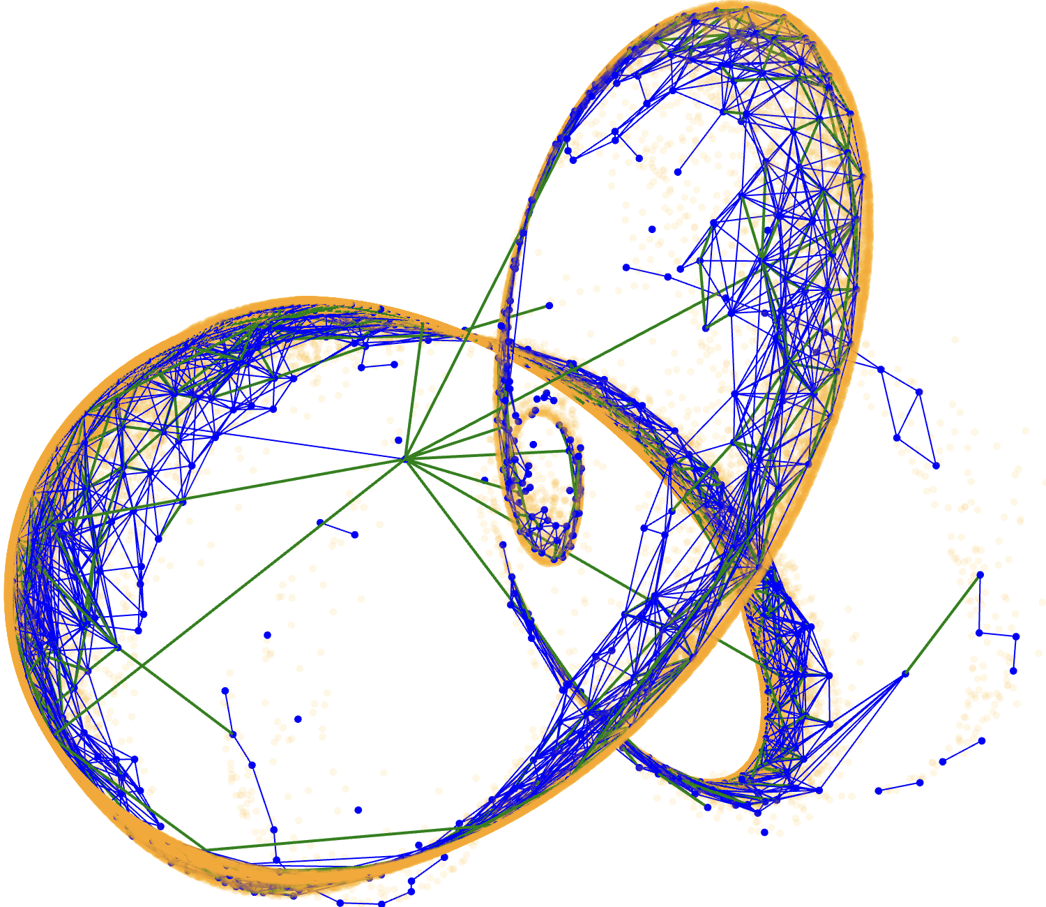
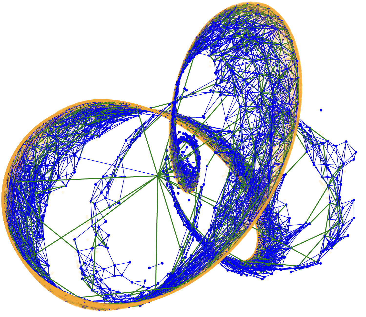
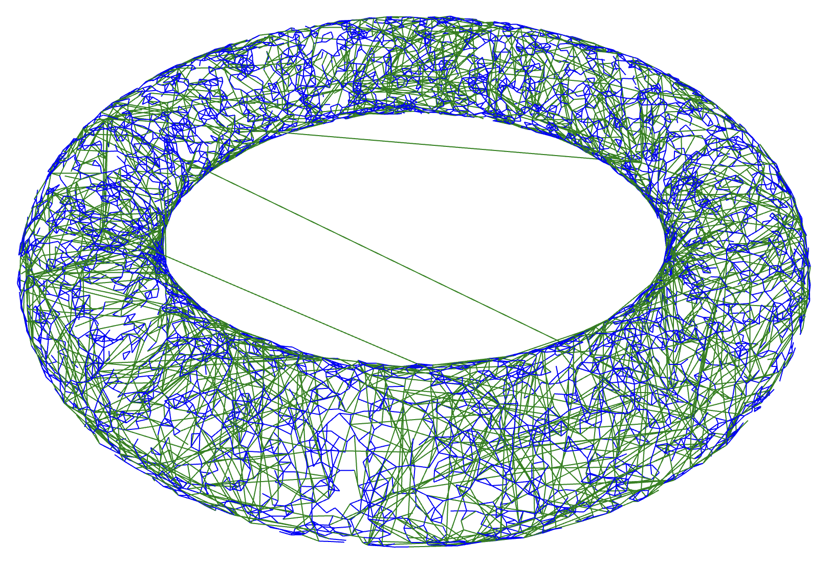
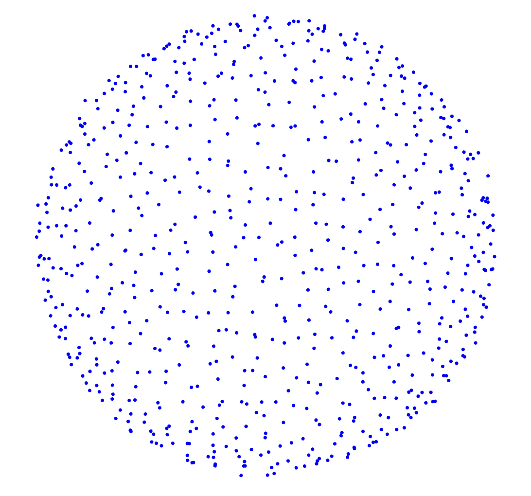
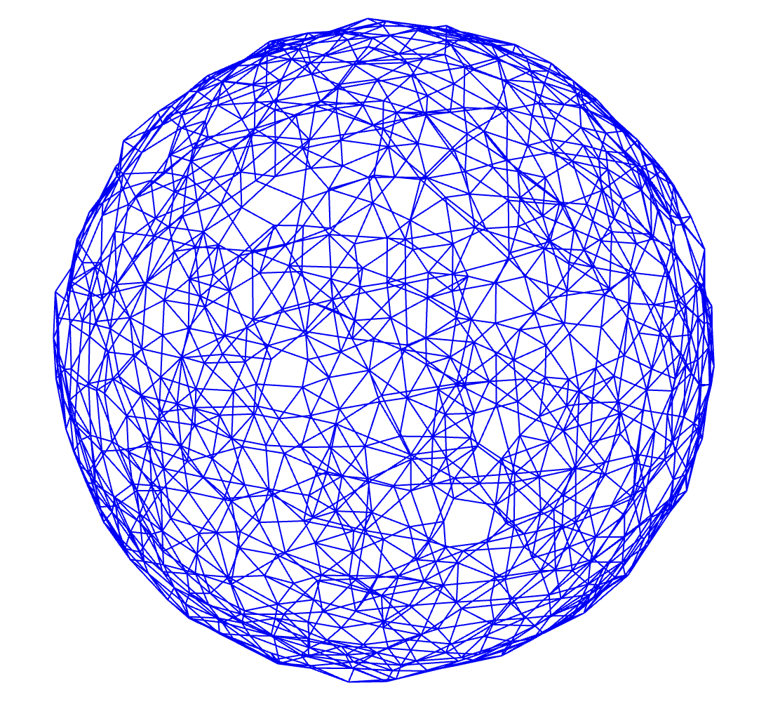
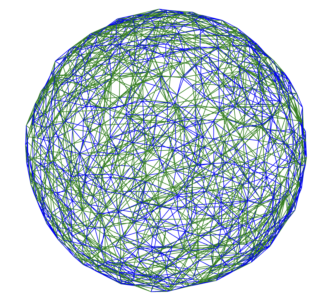
Figure 6: Growing Traversal Networks from Scientific Data. Visualization of 20482048-dimensional gravitational waves. We show clean samples (orange), landmarks (blue dots), first-order edges (blue), and zero-order edges (green). As the online algorithm sees more points, it learns an increasingly good approximation to ℳ\mathcal{M}. Number of training points: Left: 1,000. Middle: 10,000. Right: 100,000.
Algorithm 2 𝙾𝚗𝚕𝚒𝚗𝚎𝙻𝚎𝚊𝚛𝚗𝚒𝚗𝚐𝙵𝚘𝚛𝙼𝚊𝚗𝚒𝚏𝚘𝚕𝚍𝚃𝚛𝚊𝚟𝚎𝚛𝚜𝚊𝚕\mathtt{OnlineLearningForManifoldTraversal}
 Input: Current network GG, 𝐱∈ℝD\mathbf{x}\in\mathbb{R}^{D}.
 i←𝙼𝚊𝚗𝚒𝚏𝚘𝚕𝚍𝚃𝚛𝚊𝚟𝚎𝚛𝚜𝚊𝚕⁡(G,𝐱){i}\leftarrow{\mathtt{ManifoldTraversal}(G,\mathbf{x})}
 if ‖𝐪i−𝐱‖2≤R⁡(i)\|\mathbf{q}_{{i}}-\mathbf{x}\|_{2}\leq R(i) then
  Denoise via 𝐱^←𝒫𝐪i+Ti​𝐱\widehat{\mathbf{x}}\leftarrow\mathcal{P}_{\mathbf{q}_{{i}}+T_{{i}}}\mathbf{x}
  Update local parameters qi,Ti,Ξiq_{{i}},T_{{i}},\Xi_{{i}}
 else
  i⋆←arg⁡mini⁡‖𝐪i−𝐱‖2i_{\star}\leftarrow\arg\min_{i}\|\mathbf{q}_{i}-\mathbf{x}\|_{2}
  if ‖𝐪i⋆−𝐱‖2≤R⁡(i⋆)\|\mathbf{q}_{i_{\star}}-\mathbf{x}\|_{2}\leq R(i_{\star}) then
   𝐪i\mathbf{q}_{{i}} is a local min, add a zero-order edge i​→0​i⋆i\overset{0}{\rightarrow}i_{\star}
   Denoise 𝐱\mathbf{x}, update 𝐪i⋆,Ti⋆,Ξi⋆\mathbf{q}_{i_{\star}},T_{i_{\star}},\Xi_{i_{\star}}
  else
   Create a new landmark 𝐪M←𝐱\mathbf{q}_{M}\leftarrow\mathbf{x}
   Connect it to neighboring landmarks within RnbrsR_{\text{nbrs}}
   Initialize local parameters TM,ΞMT_{M},\Xi_{M}
  end if
 end if
 Output: G=(V,E)G=(V,E)

7 Theoretical Analysis

Our main theoretical result shows that the proposed mixed-order traversal method rapidly converges to a near-optimal denoised signal. We study the behavior of this method on a noisy input 𝐱=𝐱♮+𝐳\mathbf{x}=\mathbf{x}_{\natural}+\mathbf{z}, with 𝐱♮\mathbf{x}_{\natural} an arbitrary element of ℳ\mathcal{M}, and 𝐳∼iid𝒩(0,σ2)\mathbf{z}\sim_{\mathrm{iid}}\mathcal{N}(0,\sigma^{2}). Here, the goal is to produce an output 𝐱^≈𝐱♮\widehat{\mathbf{x}}\approx\mathbf{x}_{\natural} – in particular, we would like to achieve ‖𝐱^−𝐱♮‖≲σ​d\|\widehat{\mathbf{x}}-\mathbf{x}_{\natural}\|\lesssim\sigma\sqrt{d}, which is optimal for small σ\sigma.

Our analysis assumes access to an accurate collection of landmarks 𝐐={𝐪1,…,𝐪M}⊂ℳ\mathbf{Q}=\{\mathbf{q}_{1},\dots,\mathbf{q}_{M}\}\subset\mathcal{M} and their tangent spaces T𝐪iT_{\mathbf{q}_{i}}, as well as appropriately structured first-order and zero-order edge sets E1E^{1} and E0E^{0} – in a nutshell, we prove that given an appropriately structured traversal network, mixed-order traversal is both accurate and highly efficient, corroborating the conceptual picture in Figure 2.

We analyze a version (Algorithm 3) of the mixed-order method, which consists of three phases: a first-order Phase I, which, starting from an arbitrary initialization, produces an approximate critical point 𝐪iI\mathbf{q}_{i_{\mathrm{I}}}, a zero-order Phase II, which jumps to a point 𝐪iII\mathbf{q}_{i_{\mathrm{II}}} in a c​τℳc\tau_{\mathcal{M}} neighborhood of the ground truth 𝐱♮\mathbf{x}_{\natural}, followed by a first-order Phase III, produces a point 𝐪iIII\mathbf{q}_{i_{\mathrm{III}}} within distance C​κ​σ​dC\kappa\sigma\sqrt{d} of 𝐱♮\mathbf{x}_{\natural}.

𝐪\mathbf{q}𝐱1\mathbf{x}_{1}𝐱2\mathbf{x}_{2} Normal Space 𝐪+N𝐪​ℳ\mathbf{q}+N_{\mathbf{q}}\mathcal{M} 𝐪\mathbf{q} is a critical point of φ𝐱1=12​‖𝐪−𝐱1‖2\varphi_{\mathbf{x}_{1}}=\tfrac{1}{2}\|\mathbf{q}-\mathbf{x}_{1}\|^{2} and φ𝐱2=12​‖𝐪−𝐱2‖2\varphi_{\mathbf{x}_{2}}=\tfrac{1}{2}\|\mathbf{q}-\mathbf{x}_{2}\|^{2} over ℳ\mathcal{M}

Figure 7: Critical Points of the Distance Function. The point 𝐪\mathbf{q} is a critical point of the distance φ𝐱​(𝐪)=12​‖𝐪−𝐱‖22\varphi_{\mathbf{x}}(\mathbf{q})=\frac{1}{2}\|\mathbf{q}-\mathbf{x}\|_{2}^{2} for any point 𝐱\mathbf{x} satisfying 𝐱−𝐪∈N𝐪​ℳ\mathbf{x}-\mathbf{q}\in N_{\mathbf{q}}\mathcal{M}. The vista number $(ℳ)\$(\mathcal{M}) bounds the number of 𝐱\mathbf{x} for which this is true – i.e., the number of 𝐱\mathbf{x} for which 𝐪\mathbf{q} is a local minimizer. This in turn bounds the number of tunnels which must be added to ensure that local descent converges to a global optimizer. In the example illustrated here, $(ℳ)=3\$(\mathcal{M})=3.

Complexity of Escaping Suboptimal Minimizers.

A key element of Algorithm 3 (and more generally Algorithm 1) is the use of zero-order edges (or tunnels) to escape suboptimal critical points. The complexity of this step of the algorithm is dictated by the number of zero-order edges emanating from the point 𝐪iI\mathbf{q}_{i_{I}}. There is a clear geometric interpretation to this number, which is illustrated in Figure 7: a point 𝐪∈ℳ\mathbf{q}\in\mathcal{M} is a critical point of the distance function φ𝐱​(𝐪)=12​‖𝐱−𝐪‖22\varphi_{\mathbf{x}}(\mathbf{q})=\tfrac{1}{2}\|\mathbf{x}-\mathbf{q}\|_{2}^{2} if and only if 𝐱−𝐪∈N𝐪​ℳ\mathbf{x}-\mathbf{q}\in N_{\mathbf{q}}\mathcal{M}. Hence, the number of (clean) target points 𝐱♮∈ℳ\mathbf{x}_{\natural}\in\mathcal{M} for which 𝐪\mathbf{q} is a critical point is given by the number of intersections of ℳ\mathcal{M} with the normal space 𝐪+N𝐪​ℳ\mathbf{q}+N_{\mathbf{q}}\mathcal{M}. Inspired by the geometry of this picture, we denote this quantity $(ℳ)\$(\mathcal{M}):

$(ℳ)=max𝐪∈ℳ⁡#⁡[ℳ∩(𝐪+N𝐪​ℳ)].\$(\mathcal{M})=\max_{\mathbf{q}\in\mathcal{M}}\#\left[\mathcal{M}\cap(\mathbf{q}+N_{\mathbf{q}}\mathcal{M})\right]. (7.1)

Because Phase I of our algorithm produces approximate critical points, we work with a stable counterpart to this quantity: let N𝐪η​ℳ=N𝐪​ℳ+B⁡(0,η)N^{\eta}_{\mathbf{q}}\mathcal{M}=N_{\mathbf{q}}\mathcal{M}+B(0,\eta) denote an η\eta dilation of the normal space at 𝐪\mathbf{q}. We set

$rη(ℳ)=max𝐪∈ℳ⁡𝔑⁡((𝐪+N𝐪η​ℳ)∩ℳ,dℳ​(⋅,⋅),r)\$^{\eta}_{r}(\mathcal{M})=\max_{\mathbf{q}\in\mathcal{M}}\mathfrak{N}\Bigl((\mathbf{q}+N^{\eta}_{\mathbf{q}}\mathcal{M})\cap\mathcal{M},d_{\mathcal{M}}(\cdot,\cdot),r\Bigr) (7.2)

where 𝔑⁡(S,ρ,r)\mathfrak{N}(S,\rho,r) denotes the covering number of set SS in metric ρ\rho with covering radius rr. Intuitively, this counts the “number of times” the manifold intersects the dilated normal space NηN^{\eta}. As we will establish in Theorem 7.1, this quantity upper bounds the number of zero-order edges at each landmark (i.e. OPENdeg0​(𝐪))\mathrm{deg}^{0}(\mathbf{q})) required for global optimality.

Main Result.

Our main result is as follows:

Theorem 7.1.

Let ℳ⊂ℝD\mathcal{M}\subset\mathbb{R}^{D} be a complete and connected dd-dimensional manifold whose extrinsic geodesic curvature is bounded by κ\kappa. Assume κ​diam⁡(ℳ)≥1\kappa\operatorname{diam}(\mathcal{M})\geq 1 and σ​D≤c1​τℳ\sigma\sqrt{D}\leq c_{1}\tau_{\mathcal{M}}.
Assumptions on 𝐐\mathbf{Q}: The landmarks 𝐐={𝐪1,…,𝐪M}⊂ℳ\mathbf{Q}=\left\{\mathbf{q}_{1},\dots,\mathbf{q}_{M}\right\}\subset\mathcal{M} are δ\delta-separated, and form a δ\delta-net for ℳ\mathcal{M}, under the metric dℳ​(⋅,⋅)d_{\mathcal{M}}(\cdot,\cdot). Assume δ≤diam⁡ℳ\delta\leq\operatorname{diam}{\mathcal{M}}.
Assumptions on E1E^{1}: First-order graph E1E^{1} is defined such that u​↔1​v∈E1u\overset{1}{\leftrightarrow}v\in E^{1} when ‖𝐪u−𝐪v‖2≤Rnbrs\left\|\mathbf{q}_{u}-\mathbf{q}_{v}\right\|_{2}\leq R_{\text{nbrs}}. Assume a​δ=Rnbrs≤c2​σ​d{a\delta}=R_{\text{nbrs}}\leq c_{2}\sigma\sqrt{d} for some a≥40a\geq 40.
Assumptions on E0E^{0}: E0E^{0} is a minimal collection of edges satisfying the following covering property: for distinct 𝐪,𝐪′∈Q\mathbf{q},\mathbf{q}^{\prime}\in Q, if 𝐪′∈𝐪+N𝐪η​ℳ\mathbf{q}^{\prime}\in\mathbf{q}+N^{\eta}_{\mathbf{q}}\mathcal{M} with

η≥ϵ1+c4​σ​d​κ​diam⁡(ℳ)+log⁡(δ−1​diam⁡(ℳ)),\eta\geq\epsilon_{1}+c_{4}\sigma\sqrt{d}\sqrt{\kappa\operatorname{diam}(\mathcal{M})+\log(\delta^{-1}\operatorname{diam}(\mathcal{M}))},

there exists a zero-order edge 𝐪​→0​𝐪′′\mathbf{q}\overset{0}{\rightarrow}\mathbf{q}^{\prime\prime} with 𝐪′′∈Bℳ​(𝐪′,c5​τℳ)\mathbf{q}^{\prime\prime}\in B_{\mathcal{M}}(\mathbf{q}^{\prime},c_{5}\tau_{\mathcal{M}}).

With high probability in the noise 𝐳\mathbf{z}, Algorithm 3 with parameters

Ra\displaystyle R_{a} =Rnbrs−δ,\displaystyle=R_{\mathrm{nbrs}}-\delta,
ϵ1\displaystyle\epsilon_{1} >Rnbrs​(c6​κ​diam⁡(ℳ)+CLOSE\displaystyle>R_{\mathrm{nbrs}}\Bigl(c_{6}\kappa\operatorname{diam}(\mathcal{M})+
OPENc7​κ​σ​d1/2​κ​diam⁡(ℳ)+log⁡(δ−1​a​diam⁡(ℳ))),\displaystyle\quad c_{7}\kappa\sigma d^{1/2}\sqrt{\kappa\operatorname{diam}(\mathcal{M})+\log(\delta^{-1}a\operatorname{diam}(\mathcal{M}))}\Bigr),
ϵ2\displaystyle\epsilon_{2} >c8​max⁡{κ,1}​σ​d,\displaystyle>c_{8}\max\{\kappa,1\}\sigma\sqrt{d},

produces an output 𝐪⋆\mathbf{q}_{\star} satisfying dℳ​(𝐪⋆,𝐱♮)≤2​ϵ2d_{\mathcal{M}}(\mathbf{q}_{\star},\mathbf{x}_{\natural})\leq 2\epsilon_{2} with an overall number of arithmetic operations bounded by

O⁡((D+ec′​log⁡(a)​d)​(diam2⁡(ℳ)ϵ1​δ+1κ​δ)​d+D×$c6​τℳη(ℳ)).O\left((D+e^{c^{\prime}\log\left(a\right)d})\Bigl(\frac{\operatorname{diam}^{2}(\mathcal{M})}{\epsilon_{1}\delta}+\frac{1}{\kappa\delta}\Bigr)d+D\times\$^{\eta}_{c_{6}\tau_{\mathcal{M}}}(\mathcal{M})\right).

Here, τℳ\tau_{\mathcal{M}} is the reach of ℳ\mathcal{M}, i.e., the radius of the largest tubular neighborhood of ℳ\mathcal{M} where the projection 𝒫ℳ​𝐱\mathcal{P}_{\mathcal{M}}\mathbf{x} is unique (Federer, 1959). The assumption σ​D≤c1​τℳ\sigma\sqrt{D}\leq c_{1}\tau_{\mathcal{M}} ensures that, with high probability ‖𝐳‖≤τℳ\|\mathbf{z}\|\leq\tau_{\mathcal{M}}, the projection Pℳ​(𝐱)P_{\mathcal{M}}(\mathbf{x}) is close to 𝐱♮\mathbf{x}_{\natural} in the geodesic distance dℳd_{\mathcal{M}}.

The extrinsic geodesic curvature κ\kappa is the supremum of ‖γ¨‖\|\ddot{\gamma}\| over all unit speed geodesics γ⁡(t)\gamma(t) on ℳ\mathcal{M}. This quantity measures how “curvy” geodesics in ℳ\mathcal{M} are. diam⁡(ℳ)\mathrm{diam}(\mathcal{M}) is the diameter of ℳ\mathcal{M} in the intrinsic distance dℳd_{\mathcal{M}}. $c6​τℳη(ℳ)\$^{\eta}_{c_{6}\tau_{\mathcal{M}}}(\mathcal{M}) upper bounds the number of zero-order edges per landmark.

Interpretation.

This result shows that given accurate landmarks, tangent spaces, and first-order and zero-order graphs, the algorithm converges to a max⁡{κ,1}​σ​d\max\{\kappa,1\}\sigma\sqrt{d} neighborhood of x♮x_{\natural}, which is best achievable up to constant when κ\kappa is bounded. The algorithm admits an upper bound on the required number of arithmetic operations. (D​d+ec′​log⁡(a)​d​d)(Dd+e^{c^{\prime}\log\left(a\right)d}d) is the computational cost of taking one first-order step, as D​dDd comes from projection of the DD-dimensional gradient into the dd-dimensional tangent space, and d​ec′​log⁡(a)​dde^{c^{\prime}\log(a)d} represents the cost of comparing the dd-dimensional dot product between the negative Riemannian gradient with all first-order edge embeddings, with number of neighbors bounded by ec′​log⁡(a)​de^{c^{\prime}\log\left(a\right)d}.
(diam2⁡(ℳ)ϵ1​δ+1κ​δ)(\frac{\operatorname{diam}^{2}\left(\mathcal{M}\right)}{\epsilon_{1}\delta}+\frac{1}{\kappa\delta}) represent the total number of first order steps taken. diam2⁡(ℳ)ϵ1​δ\frac{\operatorname{diam}^{2}\left(\mathcal{M}\right)}{\epsilon_{1}\delta} represents the number of steps on the path from 𝐪i0\mathbf{q}_{i^{0}} (initialization) to 𝐪iI\mathbf{q}_{i_{\mathrm{I}}}. Since the initialization could be arbitrarily bad, in this phase we can only guarantee decrease in the value of φ𝐱​(𝐪)\varphi_{\mathbf{x}}(\mathbf{q}), so naturally diam2⁡(ℳ)\operatorname{diam}^{2}(\mathcal{M}) captures the worst case initialization. The ϵ1​δ{\epsilon_{1}\delta} represents the minimal decrease in each step: since the landmarks QQ forms a δ\delta-net of the manifold, each gradient direction is approximately covered, and each first order step have gradient norm at least ϵ1,\epsilon_{1}, by definition of the stopping criterion. On the other hand, 1κ​δ\frac{1}{\kappa\delta} represents the number of operations from 𝐪iII\mathbf{q}_{i_{\mathrm{II}}} to 𝐪iIII\mathbf{q}_{i_{\mathrm{III}}}. By construction 𝐪iII∈Bℳ​(𝐱♮,c5​τℳ)\mathbf{q}_{i_{\mathrm{II}}}\in B_{\mathcal{M}}(\mathbf{x}_{\natural},c_{5}\tau_{\mathcal{M}}), so when we consider dℳ​(𝐱♮,⋅)d_{\mathcal{M}}(\mathbf{x}_{\natural},\cdot) as the new objective function, the worst case initialization is 1κ\frac{1}{\kappa} and on this scale each gradient step is guaranteed to walk along the manifold, giving us a δ\delta-decrease in the intrinsic distance to 𝐱♮\mathbf{x}_{\natural}.

Finally, the D×$c6​τℳη(ℳ)D\times\$^{\eta}_{c_{6}\tau_{\mathcal{M}}}(\mathcal{M}) represents the cost of the zero order step from 𝐪iI\mathbf{q}_{i_{\mathrm{I}}}, the ϵ1\epsilon_{1}-approximate critical point for φ𝐱\varphi_{\mathbf{x}}, to 𝐪iII\mathbf{q}_{i_{\mathrm{II}}}, the point that lies intrinsically close to 𝐱♮.\mathbf{x}_{\natural}. $τℳη(ℳ)\$^{\eta}_{\tau_{\mathcal{M}}}(\mathcal{M}) is a new geometric quantity that we’ve defined, and it captures how much ℳ\mathcal{M} intersects its own dilated normal space. Intuitively larger $τℳη(ℳ)\$^{\eta}_{\tau_{\mathcal{M}}}(\mathcal{M}) means one would expect more local minimizes while performing first order descent. Notably $τℳη(ℳ)\$^{\eta}_{\tau_{\mathcal{M}}}(\mathcal{M}) can be exponential in dd in the worst case manifold, in which case our algorithm behaves similarly to nearest neighbor search. Intuitively, the parameter ϵ1\epsilon_{1} (and corresponding requirement η\eta on the zero order edges) cuts out a tradeoff between the complexity of the first order phases and the complexity of the zero order phase.

Algorithm 3 𝟷𝟶𝟷​𝚃​𝚛​𝚊​𝚟​𝚎​𝚛​𝚜​𝚊​𝚕\mathtt{101Traversal}
 Input: Network GG, 𝐱∈ℝD,Ra,ϵ1,ϵ2\mathbf{x}\in\mathbb{\mathbb{R}}^{D},R_{a},\epsilon_{1},\epsilon_{2}
 Initialization ii {Phase I\mathrm{I}}
 while ‖𝒫Ti​(𝐱−𝐪i)‖2>ϵ1\left\|\mathcal{P}_{T_{i}}(\mathbf{x}-\mathbf{q}_{i})\right\|_{2}>\epsilon_{1} do
  i←arg​minj:i​→1​j‖𝒫B⁡(0,Ra)𝒫Ti(𝐱−𝐪i)−𝒫Ti(𝐪j−𝐪i)‖2i\leftarrow\argmin\limits_{j:i\overset{1}{\rightarrow}j}\left\|\mathcal{P}_{B(0,R_{a})}\mathcal{P}_{T_{i}}(\mathbf{x}-\mathbf{q}_{i})-\mathcal{P}_{T_{i}}(\mathbf{q}_{j}-\mathbf{q}_{i})\right\|_{2}
 end while
 iI←ii_{\mathrm{I}}\leftarrow i
 iII←argminj:iI​→0​j∥𝐪j−𝐱∥2i_{\mathrm{II}}\leftarrow\arg\min_{j:i_{\mathrm{I}}\overset{0}{\rightarrow}j}\|\mathbf{q}_{j}-\mathbf{x}\|_{2} {Phase II\mathrm{II}}
 i←iIIi\leftarrow i_{\mathrm{II}} {Phase III\mathrm{III}}
 while ‖PTi​(𝐱−𝐪i)‖2>ϵ2\left\|P_{T_{i}}(\mathbf{x}-\mathbf{q}_{i})\right\|_{2}>\epsilon_{2} do
  i←arg​minj:i​→1​j‖𝒫B⁡(0,Ra)𝒫Ti(𝐱−𝐪i)−𝒫Ti(𝐪j−𝐪i)‖2i\leftarrow\argmin\limits_{j:i\overset{1}{\rightarrow}j}\left\|\mathcal{P}_{B(0,R_{a})}\mathcal{P}_{T_{i}}(\mathbf{x}-\mathbf{q}_{i})-\mathcal{P}_{T_{i}}(\mathbf{q}_{j}-\mathbf{q}_{i})\right\|_{2}
 end while
 iIII←ii_{\mathrm{III}}\leftarrow i
 Output: 𝐪iIII\mathbf{q}_{i_{\mathrm{III}}}

8 Simulations and Experiments

In this section, we visualize the traversal networks constructed using Algorithm 2 across synthetic manifolds and high-dimensional scientific data. Our experiments show that denoising performance of Algorithm 2 improves with increased number of training data, indicating that the algorithm effectively learns to denoise. Based on experiments with gravitational wave signals, we further demonstrate that Algorithm 2 achieves a better test-time complexity and accuracy tradeoff compared to Nearest Neighbor over the same set of landmarks. Additional experiments on image datasets and comparisons with autoencoders for gravitational wave denoising are detailed in Appendix K.

Traversal Network Construction for Various Manifolds.

Algorithm 2 grows the manifold traversal network, processing one sample at a time and learning tangent spaces and landmarks in the process. Figure 5 reveals the graph construction process during early training for the Swiss roll and Mobius strip (intrinsic d=2d=2, ambient D=3D=3). The figure provides visual confirmation of the fact that first-order edges (blue) capture local information (clearly visible in the Möbius strip), and zero-order edges (red) create tunnels that help escape local minimizers (clearly visible in the Swiss roll).

In addition to synthetic manifolds in ℝ3\mathbb{R}^{3}, we also grow traversal networks on high-dimensional real-world data. We learn a denoiser on a dataset of 100,000 noisy gravitational waves (Abramovici et al., 1992; Aasi et al., 2015) using the online method as described in Algorithm 2. Data are D=2048D=2048-dimensional, with intrinsic dimension d=2d=2, depicted in Figure: 6. We refer the reader to the Appendix F.1 for data generation details.

Improvement of Denoising Performance with Streaming Data.

We measure the performance of our learned denoiser on a dataset of 100,000 noisy gravitational waves. Figure 8 shows the training error of the learned denoiser. The training error across the first nn data points is given by

MSE=1n​∑i=1n‖𝐱^i−𝐱i,♮‖22\mathrm{MSE}=\frac{1}{n}\sum_{i=1}^{n}\left\|\widehat{\mathbf{x}}_{i}-\mathbf{x}_{i,\natural}\right\|_{2}^{2} (8.1)

where 𝐱^i\widehat{\mathbf{x}}_{i} is the denoised point, and 𝐱i,♮\mathbf{x}_{i,\natural} is the ground truth. We plot the theoretical lower bound as σ2​d\sigma^{2}d and see that the denoiser error decreases, showing potential to converge to the optimal theoretical lower bound.

Figure 8: Training Error: Training error decreases with the number of training points. We train a denoiser with 100,000 noisy samples with parameters R⁡(i),RnbrsR(i),R_{\text{nbrs}}. The error curve shows the potential to approach the theoretical optimal σ2​d\sigma^{2}d.

Tradeoff: Test-time efficiency vs. Denoising Performance.

We investigate the tradeoffs between performance and complexity for our mixed order method, and baselines such as nearest neighbor (NN) search. After obtaining a traversal network (Q,T,Ξ,E0,E1)(Q,T,\Xi,E^{0},E^{1}), we compare using the following experimental setup. For NN and our method, we search over the same set of landmarks QQ. We measure accuracy in mean squared error (same metric as in (8.1)) and complexity in number of multiplications. An important parameter in Algorithm 2 is the denoising radius R⁡(i)R(i) which controls the complexity by determining the number of landmarks created.

Conceptually, R⁡(i)R(i) measures distance between a noisy point 𝐱\mathbf{x} and the the landmark that best describes it. Throughout Algorithm 2, the landmark error decreases, and R⁡(i)R(i) should be reduced accordingly. Hence, we define a general formula for R⁡(i)R(i) as follows:

R⁡(i)=σ2​D+σ2​D/Ni+σ2​dR(i)=\sqrt{\sigma^{2}D+\sigma^{2}D/N_{i}+\sigma^{2}d} (8.2)

where the first error term σ2​D\sigma^{2}D comes from noisy points 𝐱i\mathbf{x}_{i}, and the second term σ2​D/Ni\sigma^{2}D/N_{i} comes from the fact that there is distance between landmarks and the true manifold. Initially, a landmark 𝐪i\mathbf{q}_{i} is created using one noisy point 𝐱\mathbf{x}. As more and more points are used to update landmark 𝐪i\mathbf{q}_{i} and other local parameters at vertex ii, local approximation gets more and more accurate, and the distance between the landmark and true manifold should decrease. This is why we divide the error σ2​D\sigma^{2}D by NiN_{i}, the number of points used to update landmark 𝐪i\mathbf{q}_{i} and other local parameters, making R⁡(i)R(i) smaller. Lastly, σ2​d\sigma^{2}d term comes from the error ‖Pℳ​𝐱−𝐱♮‖22\|P_{\mathcal{M}}\mathbf{x}-\mathbf{x}_{\natural}\|_{2}^{2} across the manifold ℳ\mathcal{M} – see Appendix J.

Figure 9 summarizes test-time accuracy versus complexity of the proposed mixed-order method, comparing it to nearest neighbor search. We do this comparison based on a test set of 20,00020,000 noisy points. By varying R⁡(i)R(i) and RnbrsR_{\mathrm{nbrs}} (see Table 1 in the Appendix for details), we obtain twelve different networks {(Qj,Tj,Ξj,Ej0,Ej1)}j=112\{(Q_{j},T_{j},\Xi_{j},E^{0}_{j},E^{1}_{j})\}_{j=1}^{12}. We compare our method of network jj with nearest neighbor search over the same set of landmarks QjQ_{j}. The details can be found in Appendix K. As shown in Figure 9, manifold traversal achieves significantly better complexity-accuracy trade-offs compared to nearest neighbor search. Figure 9 illustrates that decreasing R⁡(i)R(i), as the number of samples NiN_{i} assigned to landmark 𝐪i\mathbf{q}_{i} increases, leads to better accuracy compared to maintaining a constant radius.

Figure 9: Test-Time Complexity-Accuracy Tradeoff of Mixed-order Method versus Nearest Neighbor. Over a test set of 20,00020,000 noisy points, our proposed mixed-order method achieves better tradeoffs compared to nearest neighbor search over the same set of landmarks.

9 Conclusions

We introduced a novel framework for test-time efficient and accurate manifold denoising when the manifold is unknown and only noisy samples are given. The framework incorporates an online learning method to construct an augmented graph for optimizing on the approximated manifold, and a mixed-order method that ensures both efficiency and global optimality. Our experiments on scientific manifolds demonstrate that the proposed methods achieve a superior complexity-accuracy tradeoff vis. nearest neighbor search, which is the core of many existing provable denoising approaches. Furthermore, our analyses show that the mixed-order method attains near-optimal denoising performance, assuming the online learning method produces an ideal graph, and we provide complexity analyses for the mixed-order method under this assumption.

A promising future direction is to establish theoretical guarantees for the accuracy of the landmarks generated by the online learning method, as they play a crucial role in denoising performance. The current learning method dynamically builds edges in the graph as needed. Another potential avenue for future research is to develop a sparser network using pruning techniques while maintaining global optimality, which could further improve test-time efficiency. More broadly, we aim to leverage this designed method to study the traversal properties of natural datasets across a wide and diverse range of datasets. Additionally, integrating this method as a denoiser block within signal generation and reconstruction architectures could be a valuable direction, potentially accelerating the entire process.

Acknowledgements

The authors gratefully acknowledge support from the National Science Foundation, through the grant NSF 2112085. Shiyu Wang also gratefully acknowledges support from the Chiang Chen Industrial fellowship. The authors are grateful for the generous support of Columbia University in the City of New York. The authors would like to highlight the inspirational and community creating role of NSF’s CCF-1740391 grant. The authors thank Davit Shadunts for his contributions to refactoring and organizing the codebase used in the final version of the paper.

Impact Statement

This paper presents work whose goal is to advance the field of Machine Learning. There are many potential societal consequences of our work, none which we feel must be specifically highlighted here.

References

  • Aamari et al. (2019) Aamari, E., Kim, J., Chazal, F., Michel, B., Rinaldo, A., and Wasserman, L. Estimating the reach of a manifold. Electronic Journal of Statistics, 13(1):1359 – 1399, 2019. doi: 10.1214/19-EJS1551. URL https://doi.org/10.1214/19-EJS1551.
  • Aasi et al. (2015) Aasi, J., Abbott, B., Abbott, R., Abbott, T., Abernathy, M., Ackley, K., Adams, C., Adams, T., Addesso, P., Adhikari, R., et al. Advanced ligo. Classical and quantum gravity, 32(7):074001, 2015.
  • Abramovici et al. (1992) Abramovici, A., Althouse, W. E., Drever, R. W., Gürsel, Y., Kawamura, S., Raab, F. J., Shoemaker, D., Sievers, L., Spero, R. E., Thorne, K. S., et al. Ligo: The laser interferometer gravitational-wave observatory. science, 256(5055):325–333, 1992.
  • Absil et al. (2008) Absil, P.-A., Mahony, R., and Sepulchre, R. Optimization algorithms on matrix manifolds. Princeton University Press, 2008.
  • Adler & Taylor (2007) Adler, R. J. and Taylor, J. E. Gaussian inequalities. Random Fields and Geometry, pp. 49–64, 2007.
  • Agustsson & Timofte (2017) Agustsson, E. and Timofte, R. Ntire 2017 challenge on single image super-resolution: Dataset and study. In Proceedings of the IEEE conference on computer vision and pattern recognition workshops, pp. 126–135, 2017.
  • Arora et al. (2012) Arora, R., Cotter, A., Livescu, K., and Srebro, N. Stochastic optimization for pca and pls. In 2012 50th annual allerton conference on communication, control, and computing (allerton), pp. 861–868. IEEE, 2012.
  • Aysin et al. (1998) Aysin, B., Chaparro, L., Grave, I., and Shusterman, V. Denoising of non-stationary signals using optimized karhunen-loeve expansion. In Proceedings of the IEEE-SP International Symposium on Time-Frequency and Time-Scale Analysis (Cat. No. 98TH8380), pp. 621–624. IEEE, 1998.
  • Boucheron et al. (2003) Boucheron, S., Lugosi, G., and Bousquet, O. Concentration inequalities. In Summer school on machine learning, pp. 208–240. Springer, 2003.
  • Brand (2006) Brand, M. Fast low-rank modifications of the thin singular value decomposition. Linear algebra and its applications, 415(1):20–30, 2006.
  • Buades et al. (2005) Buades, A., Coll, B., and Morel, J.-M. A non-local algorithm for image denoising. Computer Vision and Pattern Recognition (CVPR), pp. 60–65, 2005.
  • Dabov et al. (2007) Dabov, K., Foi, A., Katkovnik, V., and Egiazarian, K. Image denoising by sparse 3-d transform-domain collaborative filtering. IEEE Transactions on Image Processing, 16(8):2080–2095, 2007.
  • Does et al. (2019) Does, M. D., Olesen, J. L., Harkins, K. D., Serradas-Duarte, T., Gochberg, D. F., Jespersen, S. N., and Shemesh, N. Evaluation of principal component analysis image denoising on multi-exponential mri relaxometry. Magnetic resonance in medicine, 81(6):3503–3514, 2019.
  • Donoho (1995) Donoho, D. L. De-noising by soft-thresholding. IEEE Transactions on Information Theory, 41(3):613–627, 1995.
  • Elad & Aharon (2006) Elad, M. and Aharon, M. Image denoising via sparse and redundant representations over learned dictionaries. IEEE Transactions on Image Processing, 15(12):3736–3745, 2006.
  • Fan et al. (2022) Fan, C.-M., Liu, T.-J., and Liu, K.-H. Sunet: Swin transformer unet for image denoising. In 2022 IEEE International Symposium on Circuits and Systems (ISCAS), pp. 2333–2337. IEEE, 2022.
  • Federer (1959) Federer, H. Curvature measures. Transactions of the American Mathematical Society, 93(3):418–491, 1959.
  • Fefferman et al. (2016) Fefferman, C., Mitter, S., and Narayanan, H. Testing the manifold hypothesis. Journal of the American Mathematical Society, 29(4):983–1049, 2016.
  • Fefferman et al. (2020) Fefferman, C., Ivanov, S., Kurylev, Y., Lassas, M., and Narayanan, H. Reconstruction and interpolation of manifolds. i: The geometric whitney problem. Foundations of Computational Mathematics, 20(5):1035–1133, 2020.
  • Genovese et al. (2012) Genovese, C. R., Perone Pacifico, M., Isabella, V., Wasserman, L., et al. Minimax manifold estimation. Journal of machine learning research, 13:1263–1291, 2012.
  • Gong et al. (2010) Gong, D., Sha, F., and Medioni, G. Locally linear denoising on image manifolds. In Proceedings of the Thirteenth International Conference on Artificial Intelligence and Statistics, pp. 265–272. JMLR Workshop and Conference Proceedings, 2010.
  • Hein & Maier (2006) Hein, M. and Maier, M. Manifold denoising. Advances in neural information processing systems, 19, 2006.
  • Ho et al. (2020) Ho, J., Jain, A., and Abbeel, P. Denoising diffusion probabilistic models. Advances in neural information processing systems, 33:6840–6851, 2020.
  • Ilesanmi & Ilesanmi (2021) Ilesanmi, A. E. and Ilesanmi, T. O. Methods for image denoising using convolutional neural network: a review. Complex & Intelligent Systems, 7(5):2179–2198, 2021.
  • Leobacher & Steinicke (2021) Leobacher, G. and Steinicke, A. Existence, uniqueness and regularity of the projection onto differentiable manifolds. Annals of global analysis and geometry, 60(3):559–587, 2021.
  • Malkov & Yashunin (2018) Malkov, Y. A. and Yashunin, D. A. Efficient and robust approximate nearest neighbor search using hierarchical navigable small world graphs. IEEE transactions on pattern analysis and machine intelligence, 42(4):824–836, 2018.
  • Nitz et al. (2023) Nitz, A., Harry, I., Brown, D., Biwer, C. M., Willis, J., Dal Canton, T., Capano, C., Dent, T., Pekowsky, L., De, S., et al. gwastro/pycbc: v2. 1.1 release of pycbc. Zenodo, 2023.
  • Sato (2021) Sato, H. Riemannian optimization and its applications, volume 670. Springer, 2021.
  • Shustin et al. (2022) Shustin, B., Avron, H., and Sober, B. Manifold free riemannian optimization. arXiv preprint arXiv:2209.03269, 2022.
  • Sober & Levin (2020) Sober, B. and Levin, D. Manifold approximation by moving least-squares projection (mmls). Constructive Approximation, 52(3):433–478, 2020.
  • Sober et al. (2020) Sober, B., Ravier, R., and Daubechies, I. Approximating the riemannian metric from point clouds via manifold moving least squares, 2020.
  • Song & Ermon (2019) Song, Y. and Ermon, S. Generative modeling by estimating gradients of the data distribution. Advances in neural information processing systems, 32, 2019.
  • Tenenbaum et al. (2000) Tenenbaum, J. B., Silva, V. d., and Langford, J. C. A global geometric framework for nonlinear dimensionality reduction. science, 290(5500):2319–2323, 2000.
  • Venkatakrishnan et al. (2013) Venkatakrishnan, S. V., Bouman, C. A., and Wohlberg, B. Plug-and-play priors for model based reconstruction. In 2013 IEEE global conference on signal and information processing, pp. 945–948. IEEE, 2013.
  • Vershynin (2018) Vershynin, R. High-dimensional probability: An introduction with applications in data science, volume 47. Cambridge university press, 2018.
  • Vincent et al. (2008) Vincent, P., Larochelle, H., Bengio, Y., and Manzagol, P.-A. Extracting and composing robust features with denoising autoencoders. In Proceedings of the 25th international conference on Machine learning, pp. 1096–1103, 2008.
  • Wiener (1949) Wiener, N. Extrapolation, Interpolation, and Smoothing of Stationary Time Series. MIT Press, 1949.
  • Yan* et al. (2023) Yan*, J., Wang*, S., Wei, X. R., Wang, J., Márka, Z., Márka, S., and Wright, J. Tpopt: Efficient trainable template optimization on low-dimensional manifolds. arXiv preprint arXiv:2310.10039, 2023. Submitted to IEEE Transactions on Signal Processing.
  • Yao et al. (2022) Yao, C., Jin, S., Liu, M., and Ban, X. Dense residual transformer for image denoising. Electronics, 11(3):418, 2022.
  • Yao et al. (2023) Yao, Z., Su, J., Li, B., and Yau, S.-T. Manifold fitting, 2023.
  • Zhang et al. (2021) Zhang, K., Zuo, W., and Zhang, L. Plug-and-play image restoration with deep denoiser prior. IEEE Transactions on Pattern Analysis and Machine Intelligence, 2021.

Appendix

Appendix A Main Claims

Theorem A.1.

Let ℳ⊂ℝD\mathcal{M}\subset\mathbb{R}^{D} be a complete and connected dd-dimensional manifold whose extrinsic geodesic curvature is bounded by κ\kappa.

  • •

    Assumptions on ℳ\mathcal{M} Assume κ​diam⁡(ℳ)≥1\kappa\operatorname{diam}(\mathcal{M})\geq 1 and σ​D≤1640​τℳ\sigma\sqrt{D}\leq\frac{1}{640}\tau_{\mathcal{M}}.

  • •

    Assumptions on QQ Suppose that the landmarks Q={𝐪1,…,𝐪M}⊂ℳQ=\left\{\mathbf{q}_{1},\dots,\mathbf{q}_{M}\right\}\subset\mathcal{M} are δ\delta-separated, and form a δ\delta-net for ℳ\mathcal{M}, under the metric dℳ​(⋅,⋅)d_{\mathcal{M}}(\cdot,\cdot). Assume δ≤diam⁡(ℳ)\delta\leq\operatorname{diam}(\mathcal{M}).

  • •

    Assumptions on E1E^{1} First-order graph E1E^{1} is defined such that u​→1​v∈E1u\overset{1}{\rightarrow}v\in E^{1} when ‖𝐪u−𝐪v‖2≤Rnbrs\left\|\mathbf{q}_{u}-\mathbf{q}_{v}\right\|_{2}\leq R_{\text{nbrs}}. Assume a​δ=Rnbrs≤264​σ​d{a\delta}=R_{\text{nbrs}}\leq\frac{\sqrt{2}}{64}\sigma\sqrt{d} for some a≥40a\geq 40.

  • •

    Assumptions on E0E^{0} E0E^{0} is a minimal collection of edges satisfying the following covering property: for distinct 𝐪,𝐪′∈Q\mathbf{q},\mathbf{q}^{\prime}\in Q, if 𝐪′∈𝐪+N𝐪η​ℳ\mathbf{q}^{\prime}\in\mathbf{q}+N^{\eta}_{\mathbf{q}}\mathcal{M} with

    η≥ϵ1+δ+14​σ​d​κ​diam⁡(ℳ)+log⁡(diam⁡(ℳ))−log⁡(δ)+log⁡(7),\eta\geq\epsilon_{1}+\delta+14\sigma\sqrt{d}\sqrt{\kappa\operatorname{diam}(\mathcal{M})+\log(\operatorname{diam}(\mathcal{M}))-\log(\delta)+\log(7)}, (A.1)

    there exists a ZOE 𝐪​→0​𝐪′′\mathbf{q}\overset{0}{\rightarrow}\mathbf{q}^{\prime\prime} with 𝐪′′∈Bℳ​(𝐪′,180​τℳ)\mathbf{q}^{\prime\prime}\in B_{\mathcal{M}}(\mathbf{q}^{\prime},\frac{1}{80}\tau_{\mathcal{M}}).

With probability at least 1−4​e−d16−(e2)−D21-4e^{-\frac{d}{16}}-\left(\frac{e}{2}\right)^{-\frac{D}{2}} in the noise 𝐳\mathbf{z}, the Algorithm 3 with parameters

Ra\displaystyle R_{a} =Rnbrs−δ\displaystyle=R_{\mathrm{nbrs}}-\delta (A.2)
ϵ1\displaystyle\epsilon_{1} >2​Rnbrs0.55​(23+83​κ​diam⁡(ℳ)+CLOSE\displaystyle>\frac{2R_{\text{nbrs}}}{0.55}\left(\frac{2}{3}+\frac{8}{3}\kappa\operatorname{diam}(\mathcal{M})+\right. (A.3)
OPEN+16​κ​σ​d​κ​diam⁡(ℳ)+log⁡(a)−log⁡(δ)+log⁡(diam⁡(ℳ))+log⁡(100))\displaystyle\qquad\qquad\left.+16\kappa\sigma\sqrt{d}\sqrt{\kappa\operatorname{diam}(\mathcal{M})+\log(a)-\log(\delta)+\log(\operatorname{diam}(\mathcal{M}))+\log(100)}\right) (A.4)
ϵ2\displaystyle\epsilon_{2} >C​max⁡{κ,1}​σ​d\displaystyle>C\max\{\kappa,1\}\sigma\sqrt{d} (A.5)

produces an output 𝐪⋆\mathbf{q}_{\star} satisfying

dℳ​(𝐪⋆,𝐱♮)≤2​ϵ2d_{\mathcal{M}}(\mathbf{q}_{\star},\mathbf{x}_{\natural})\leq 2\epsilon_{2} (A.6)

with an overall number of arithmetic operations bounded by

(D​d+d​(1+4​2​a​e)d)​(10​d​i​a​m2​(ℳ)+20​σ2​Dϵ1​δ+8κ​δ)+D×$1160​τℳη(ℳ)\left(Dd+d\left(1+4\sqrt{2}ae\right)^{d}\right)\left(\frac{10\mathrm{diam}^{2}(\mathcal{M})+20\sigma^{2}D}{\epsilon_{1}\delta}+\frac{8}{\kappa\delta}\right)+D\times\$^{\eta}_{\frac{1}{160}\tau_{\mathcal{M}}}(\mathcal{M}) (A.7)

where $rη(ℳ)\$^{\eta}_{r}(\mathcal{M}) follows the definition in Equation 7.2.

Proof. With the above assumptions and the combination of Proposition A.3, Proposition A.4, and Proposition A.5, it’s easy to show that with probability at least 1−4​e−d16−(e2)−D21-4e^{-\frac{d}{16}}-\left(\frac{e}{2}\right)^{-\frac{D}{2}} in the noise 𝐳\mathbf{z}, the output of the algorithm 𝐪⋆\mathbf{q}_{\star} satisfies

dℳ​(𝐪⋆,𝐱♮)≤2​ϵ2,d_{\mathcal{M}}(\mathbf{q}_{\star},\mathbf{x}_{\natural})\leq 2\epsilon_{2}, (A.8)

and phase I\mathrm{I} and phase III\mathrm{III} use at most diam2⁡(ℳ)+2​σ2​D0.1375​ϵ1​δ+8κ​δ\frac{\operatorname{diam}^{2}(\mathcal{M})+2\sigma^{2}D}{0.1375\epsilon_{1}\delta}+\frac{8}{\kappa\delta} steps, and phase II\mathrm{II} takes at most D×$1160​τℳη(ℳ)D\times\$^{\eta}_{\frac{1}{160}\tau_{\mathcal{M}}}(\mathcal{M}) operations.

Suppose S𝐪,η⊂ℳS_{\mathbf{q},\eta}\subset\mathcal{M} is the minimal set that 1160​τℳ\frac{1}{160}\tau_{\mathcal{M}}-covers the (𝐪+N𝐪η)∩ℳ(\mathbf{q}+N_{\mathbf{q}}^{\eta})\cap\mathcal{M} under the metric dℳ​(⋅,⋅)d_{\mathcal{M}}(\cdot,\cdot), with η≥ϵ1+δ+σ⁡(4​log⁡|𝒬|+10​d)\eta\geq\epsilon_{1}+\delta+\sigma\left(4\sqrt{\log\left|\mathcal{Q}\right|}+10\sqrt{d}\right). From the definition that $rη(ℳ)=max𝐪∈ℳ⁡𝔑⁡((𝐪+N𝐪η​ℳ)∩ℳ,dℳ​(⋅,⋅),r)\$^{\eta}_{r}(\mathcal{M})=\max_{\mathbf{q}\in\mathcal{M}}\mathfrak{N}\Bigl((\mathbf{q}+N^{\eta}_{\mathbf{q}}\mathcal{M})\cap\mathcal{M},d_{\mathcal{M}}(\cdot,\cdot),r\Bigr), where 𝔑⁡(S,ρ,r)\mathfrak{N}(S,\rho,r) denotes the covering number of set SS in metric ρ\rho with covering radius rr, we have OPEN|S𝐪,η|=𝔑⁡((𝐪+N𝐪η)∩ℳ),dℳ​(⋅,⋅),1160​τℳ)≤$1160​τℳη|S_{\mathbf{q},\eta}|=\mathfrak{N}\Bigl((\mathbf{q}+N^{\eta}_{\mathbf{q}})\cap\mathcal{M}),d_{\mathcal{M}}(\cdot,\cdot),\frac{1}{160}\tau_{\mathcal{M}}\Bigr)\leq\$_{\frac{1}{160}\tau_{\mathcal{M}}}^{\eta}.

For any 𝐪∈𝒬\mathbf{q}\in\mathcal{Q}, as the landmark 𝒬\mathcal{Q} δ\delta-covers the manifold, it δ\delta-covers S𝐪,ηS_{\mathbf{q},\eta}. We denote the minimal set of landmarks that δ\delta-cover S𝐪,ηS_{\mathbf{q},\eta} as 𝒬S\mathcal{Q}_{S}. Then for any 𝒒′∈𝒬,𝐪′∈𝐪+N𝐪η\bm{q}^{\prime}\in\mathcal{Q},\mathbf{q}^{\prime}\in\mathbf{q}+N^{\eta}_{\mathbf{q}}, there exists a point 𝐬∈S𝐪,η\mathbf{s}\in S_{\mathbf{q},\eta} such that dℳ​(𝐬,𝐪′)≤1160​τℳd_{\mathcal{M}}(\mathbf{s},\mathbf{q}^{\prime})\leq\frac{1}{160}\tau_{\mathcal{M}}. Since 𝐬∈S𝐪,η\mathbf{s}\in S_{\mathbf{q},\eta}, there exists a landmark 𝐪′′∈𝒬S\mathbf{q}^{\prime\prime}\in\mathcal{Q}_{S} such that dℳ​(𝐬,𝐪′′)≤δd_{\mathcal{M}}(\mathbf{s},\mathbf{q}^{\prime\prime})\leq\delta.

Therefore, for any 𝐪′∈𝐪+N𝐪η\mathbf{q}^{\prime}\in\mathbf{q}+N^{\eta}_{\mathbf{q}}, there exists 𝒒′′∈𝒬S\bm{q}^{\prime\prime}\in\mathcal{Q}_{S} such that

dℳ​(𝐪′,𝐪′′)≤dℳ​(𝐪′,𝐬)+dℳ​(𝐬,𝐪′′)≤1160​τℳ+δ≤1160​τℳ+240∗64∗640​τℳ≤180​τℳ,d_{\mathcal{M}}(\mathbf{q}^{\prime},\mathbf{q}^{\prime\prime})\leq d_{\mathcal{M}}(\mathbf{q}^{\prime},\mathbf{s})+d_{\mathcal{M}}(\mathbf{s},\mathbf{q}^{\prime\prime})\\ \leq\frac{1}{160}\tau_{\mathcal{M}}+\delta\\ \leq\frac{1}{160}\tau_{\mathcal{M}}+\frac{\sqrt{2}}{40*64*640}\tau_{\mathcal{M}}\leq\frac{1}{80}\tau_{\mathcal{M}}, (A.9)

where we used δ=Rnbrsa\delta=\frac{R_{\mathrm{nbrs}}}{a}, a≥40a\geq 40, Rnbrs≤264​σ​dR_{\mathrm{nbrs}}\leq\frac{\sqrt{2}}{64}\sigma\sqrt{d}, d≤Dd\leq D, and σ​D≤1640​τℳ\sigma\sqrt{D}\leq\frac{1}{640}\tau_{\mathcal{M}} assumed in Theorem A.1 from the third-to-last step to the second-to-last step.

As a result, the set {𝐪​→0​𝐪′′∣∀𝐪′′∈𝒬S}\left\{\mathbf{q}\overset{0}{\rightarrow}\mathbf{q}^{\prime\prime}\mid\forall\mathbf{q}^{\prime\prime}\in\mathcal{Q}_{S}\right\} satisfies the covering property in the assumption on E0E^{0}. Since E0E^{0} is the minimum collection that satisfies this covering property, the number of zero-order edges at 𝐪\mathbf{q}, i.e., deg0⁡(𝐪)\deg^{0}(\mathbf{q}) satisfies

deg0⁡(𝐪)≤|{𝐪​→0​𝐪′′∣∀𝐪′′∈𝒬S}|≤|S𝐪,η|≤$1160​τℳη.\deg^{0}(\mathbf{q})\leq\left|\left\{\mathbf{q}\overset{0}{\rightarrow}\mathbf{q}^{\prime\prime}\mid\forall\mathbf{q}^{\prime\prime}\in\mathcal{Q}_{S}\right\}\right|\leq\left|S_{\mathbf{q},\eta}\right|\leq\$^{\eta}_{\frac{1}{160}\tau_{\mathcal{M}}}. (A.10)

And we note that projection of the gradient onto the tangent space takes the cost of D∗dD*d number of operations, and choosing the first-order neighbor takes the cost of d∗max𝒒u∈𝒬⁡|Eu1|d*\max_{\bm{q}_{u}\in\mathcal{Q}}\left|E_{u}^{1}\right|. The number of arithmetic operations of zero-order step is D∗max𝐪∈Q⁡deg0⁡(𝐪)D*\max_{\mathbf{q}\in Q}\deg^{0}(\mathbf{q}), where DD comes from the Euclidean distance calculation, and max𝐪∈Q⁡deg0⁡(𝐪)\max_{\mathbf{q}\in Q}\deg^{0}(\mathbf{q}) is bounded by the defined geometric quantity $1160​τℳη(ℳ)\$^{\eta}_{\frac{1}{160}\tau_{\mathcal{M}}}(\mathcal{M}). Combined all of terms above, we end up with the bound on the number of operations performed by our algorithm.  

Fact A.2.

For a manifold ℳ\mathcal{M} with reach τℳ\tau_{\mathcal{M}} and extrinsic curvature bounded by κ\kappa, we have

τℳ≤1/κ.\tau_{\mathcal{M}}\leq 1/\kappa. (A.11)

See Proposition 2.3 in (Aamari et al., 2019). We used this fact directly in the following proofs.

Proposition A.3.

Let ℳ⊂ℝD\mathcal{M}\subset\mathbb{R}^{D} be a complete and connected dd-dimensional manifold whose extrinsic geodesic curvature is bounded by κ\kappa. Suppose the landmarks {𝐪u}\{\mathbf{q}_{u}\} are δ\delta-separated, and form a δ\delta-net for ℳ\mathcal{M}, and that the first order graph E1E^{1} satisfies u​→1​v∈E1u\overset{1}{\rightarrow}v\in E^{1} when ‖𝐪u−𝐪v‖2≤Rnbrs\|\mathbf{q}_{u}-\mathbf{q}_{v}\|_{2}\leq R_{\mathrm{nbrs}}, and that 40​δ≤Rnbrs≤τℳ40\delta\leq R_{\text{nbrs}}\leq\tau_{\mathcal{M}}. Assume δ≤diam⁡(ℳ)\delta\leq\operatorname{diam}(\mathcal{M}) and κ​diam⁡(ℳ)≥1\kappa\operatorname{diam}(\mathcal{M})\geq 1. Then with probability at least

1−e−9​d2−(e2)−D21-e^{-\frac{9d}{2}}-\left(\frac{e}{2}\right)^{-\frac{D}{2}} (A.12)

in the noise 𝐳\mathbf{z}, the first phase of first-order optimization in Algorithm 3 with parameters

Ra\displaystyle R_{a} =Rnbrs−δ,\displaystyle=R_{\text{nbrs}}-\delta, (A.13)
ϵ1\displaystyle\epsilon_{1} >2​Rnbrs0.55​(23+83​κ​diam⁡(ℳ)+CLOSE\displaystyle>\frac{2R_{\text{nbrs}}}{0.55}\left(\frac{2}{3}+\frac{8}{3}\kappa\operatorname{diam}(\mathcal{M})+\right. (A.14)
OPEN+16​κ​σ​d​κ​diam⁡(ℳ)+log⁡(a)−log⁡(δ)+log⁡(diam⁡(ℳ))+log⁡(100)),\displaystyle\qquad\qquad\left.+16\kappa\sigma\sqrt{d}\sqrt{\kappa\operatorname{diam}(\mathcal{M})+\log(a)-\log(\delta)+\log(\operatorname{diam}(\mathcal{M}))+\log(100)}\right), (A.15)

produces 𝐪iI\mathbf{q}_{i_{\mathrm{I}}} satisfying

grad⁡[φ𝐱]​(𝐪iI)=‖𝒫TiI​(𝐱−𝐪iI)‖2≤ϵ1\grad[\varphi_{\mathbf{x}}](\mathbf{q}_{i_{\mathrm{I}}})=\|\mathcal{P}_{T_{i_{\mathrm{I}}}}(\mathbf{x}-\mathbf{q}_{i_{\mathrm{I}}})\|_{2}\leq\epsilon_{1} (A.17)

using at most

diam2⁡(ℳ)+2​σ2​D0.1375​ϵ1​δ\frac{\operatorname{diam}^{2}(\mathcal{M})+2\sigma^{2}D}{0.1375\epsilon_{1}\delta} (A.18)

steps.

Proof.

We can bound the total number of steps by dividing maximum initial distance by the minimal distance decrease over each first-order step.

We note that

φ𝐱​(𝐪i0)\displaystyle\varphi_{\mathbf{x}}(\mathbf{q}_{i^{0}}) =12​‖𝐪i0−𝐱‖22\displaystyle=\frac{1}{2}\left\|\mathbf{q}_{i^{0}}-\mathbf{x}\right\|_{2}^{2} (A.19)
≤‖𝐪i0−𝐱♮‖22+‖𝐳‖22\displaystyle\leq\left\|\mathbf{q}_{i^{0}}-\mathbf{x}_{\natural}\right\|_{2}^{2}+\left\|\mathbf{z}\right\|_{2}^{2}
≤diam2​(ℳ)+‖𝐳‖22\displaystyle\leq\text{diam}^{2}(\mathcal{M})+\left\|\mathbf{z}\right\|_{2}^{2}

We let 𝐳¯\mathbf{\bar{z}} be the standard unit variance Gaussian variable, for any 0<t<1/20<t<1/2, we have

ℙ[‖𝐳‖22≥2σ2D]\displaystyle\mathbb{P}[\left\|\mathbf{z}\right\|_{2}^{2}\geq 2\sigma^{2}D] =ℙ[‖𝐳¯‖22≥2D]\displaystyle=\mathbb{P}[\left\|\mathbf{\bar{z}}\right\|_{2}^{2}\geq 2D] (A.20)
=ℙ[et​‖𝐳¯‖22≥e2​t​D]\displaystyle=\mathbb{P}[e^{t\left\|\mathbf{\bar{z}}\right\|_{2}^{2}}\geq e^{2tD}]
≤𝔼⁡[et​‖𝐳¯‖22]e2​t​D\displaystyle\leq\frac{\mathbb{E}[e^{t\left\|\mathbf{\bar{z}}\right\|_{2}^{2}}]}{e^{2tD}}
=e−2​t​D(1−2​t)D2,\displaystyle=\frac{e^{-2tD}}{(1-2t)^{\frac{D}{2}}},

where we used Markov’s inequality from the second line to the third line. In particular, we can pick t=14t=\frac{1}{4}, so with probability at least 1−(e2)−D21-(\frac{e}{2})^{-\frac{D}{2}} in the noise 𝐳\mathbf{z}, we have

φ𝐱​(𝐪i0)≤diam2​(ℳ)+2​σ2​D.\varphi_{\mathbf{x}}(\mathbf{q}_{i^{0}})\leq\text{diam}^{2}(\mathcal{M})+2\sigma^{2}D. (A.21)

Now we will analyze the decrease over each first-order step from uu to u+u^{+}. We have

φ𝐱​(𝐪u+)−φ𝐱​(𝐪u)\displaystyle\varphi_{\mathbf{x}}(\mathbf{q}_{u^{+}})-\varphi_{\mathbf{x}}(\mathbf{q}_{u}) =12​(‖𝐱−𝐪u+‖22−‖𝐱−𝐪u‖22)\displaystyle=\frac{1}{2}(\|\mathbf{x}-\mathbf{q}_{u^{+}}\|_{2}^{2}-\|\mathbf{x}-\mathbf{q}_{u}\|_{2}^{2}) (A.22)
=12​‖𝐪u+−𝐪u‖22−⟨𝒫Tu​(𝐱−𝐪u),𝒫Tu​(𝐪u+−𝐪u)⟩−⟨𝒫Nu​(𝐱−𝐪u),𝒫Nu​(𝐪u+−𝐪u)⟩.\displaystyle=\frac{1}{2}\|\mathbf{q}_{u^{+}}-\mathbf{q}_{u}\|_{2}^{2}-\left\langle\mathcal{P}_{T_{u}}(\mathbf{x}-\mathbf{q}_{u}),\mathcal{P}_{T_{u}}(\mathbf{q}_{u^{+}}-\mathbf{q}_{u})\right\rangle-\left\langle\mathcal{P}_{N_{u}}(\mathbf{x}-\mathbf{q}_{u}),\mathcal{P}_{N_{u}}(\mathbf{q}_{u^{+}}-\mathbf{q}_{u})\right\rangle.

We apply Lemma B.1 to bound the first term and Lemma B.8 to get a high probability bound on the last term, setting t=3​σ​dt=3\sigma\sqrt{d}.

Next, we apply Lemma B.3and Lemma B.4 to bound the second term, which dominates the decrease in the values of the objective function after taking a first-order step. As a reminder, the step rule in Algorithm 3 is

u+=arg⁡minu​→1​v⁡‖𝒫B⁡(0,Ra)​𝒫Tu​(𝐱−𝐪u)−𝒫Tu​(𝐪v−𝐪u)‖2.u^{+}=\arg\min_{u\overset{1}{\rightarrow}v}\left\|\mathcal{P}_{B(0,R_{a})}\mathcal{P}_{T_{u}}(\mathbf{x}-\mathbf{q}_{u})-\mathcal{P}_{T_{u}}(\mathbf{q}_{v}-\mathbf{q}_{u})\right\|_{2}. (A.23)

We observe that before phase I in Algorithm 3 terminates, ‖𝒫Tu​(𝐱−𝐪u)‖≥ϵ1>Ra\left\|\mathcal{P}_{T_{u}}(\mathbf{x}-\mathbf{q}_{u})\right\|\geq\epsilon_{1}>R_{a} holds. Then the step rule is equivalent to

u+=arg⁡minu​→1​v⁡‖𝒫Tu​(𝐱−𝐪u)‖𝒫Tu​(𝐱−𝐪u)‖2​Ra−𝒫Tu​(𝐪v−𝐪u)‖2,u^{+}=\arg\min_{u\overset{1}{\rightarrow}v}\left\|\frac{\mathcal{P}_{T_{u}}\left(\mathbf{x}-\mathbf{q}_{u}\right)}{\|\mathcal{P}_{T_{u}}\left(\mathbf{x}-\mathbf{q}_{u}\right)\|_{2}}R_{a}-\mathcal{P}_{T_{u}}(\mathbf{q}_{v}-\mathbf{q}_{u})\right\|_{2}, (A.24)

in which we have ‖𝒫Tu​(𝐱−𝐪u)‖𝒫Tu​(𝐱−𝐪u)‖2​Ra‖2=Ra\left\|\frac{\mathcal{P}_{T_{u}}\left(\mathbf{x}-\mathbf{q}_{u}\right)}{\|\mathcal{P}_{T_{u}}\left(\mathbf{x}-\mathbf{q}_{u}\right)\|_{2}}R_{a}\right\|_{2}=R_{a}. Applying Lemma B.3, there exists u​→1​v∈E1u\overset{1}{\rightarrow}v\in E^{1}, such that ‖𝒫Tu​(𝐱−𝐪u)‖𝒫Tu​(𝐱−𝐪u)‖2​Ra−𝒫Tu​(𝐪v−𝐪u)‖2≤δ+12​κ​Ra2\left\|\frac{\mathcal{P}_{T_{u}}\left(\mathbf{x}-\mathbf{q}_{u}\right)}{\|\mathcal{P}_{T_{u}}\left(\mathbf{x}-\mathbf{q}_{u}\right)\|_{2}}R_{a}-\mathcal{P}_{T_{u}}(\mathbf{q}_{v}-\mathbf{q}_{u})\right\|_{2}\leq\delta+\frac{1}{2}\kappa R_{a}^{2}. From the construction of this step rule, we have ‖𝒫Tu​(𝐱−𝐪u)‖𝒫Tu​(𝐱−𝐪u)‖2​Ra−𝒫Tu​(𝐪u+−𝐪u)‖2≤‖𝒫Tu​(𝐱−𝐪u)‖𝒫Tu​(𝐱−𝐪u)‖2​Ra−𝒫Tu​(𝐪v−𝐪u)‖2≤δ+12​κ​Ra2\left\|\frac{\mathcal{P}_{T_{u}}\left(\mathbf{x}-\mathbf{q}_{u}\right)}{\|\mathcal{P}_{T_{u}}\left(\mathbf{x}-\mathbf{q}_{u}\right)\|_{2}}R_{a}-\mathcal{P}_{T_{u}}(\mathbf{q}_{u^{+}}-\mathbf{q}_{u})\right\|_{2}\leq\left\|\frac{\mathcal{P}_{T_{u}}\left(\mathbf{x}-\mathbf{q}_{u}\right)}{\|\mathcal{P}_{T_{u}}\left(\mathbf{x}-\mathbf{q}_{u}\right)\|_{2}}R_{a}-\mathcal{P}_{T_{u}}(\mathbf{q}_{v}-\mathbf{q}_{u})\right\|_{2}\leq\delta+\frac{1}{2}\kappa R_{a}^{2}. Thus when 𝐱≠𝐪u\mathbf{x}\neq\mathbf{q}_{u}, applying Lemma B.4, we have ⟨𝒫Tu​(𝐱−𝐪u),𝒫Tu​(𝐪v−𝐪u)⟩≥0.55​‖𝒫Tu​(𝐱−𝐪u)‖2​‖𝒫Tu​(𝐪v−𝐪u)‖2\left\langle\mathcal{P}_{T_{u}}\left(\mathbf{x}-\mathbf{q}_{u}\right),\mathcal{P}_{T_{u}}\left(\mathbf{q}_{v}-\mathbf{q}_{u}\right)\right\rangle\geq 0.55\|\mathcal{P}_{T_{u}}\left(\mathbf{x}-\mathbf{q}_{u}\right)\|_{2}\|\mathcal{P}_{T_{u}}\left(\mathbf{q}_{v}-\mathbf{q}_{u}\right)\|_{2}.

Combining all the above results, we conclude that with probability at least 1−e−9​d21-e^{-\frac{9d}{2}} in the noise 𝒛\bm{z}, we have

φ𝐱​(𝐪u+)−φ𝐱​(𝐪u)\displaystyle\varphi_{\mathbf{x}}(\mathbf{q}_{u^{+}})-\varphi_{\mathbf{x}}(\mathbf{q}_{u}) ≤23​‖𝒫Tu​(𝐪u+−𝐪u)‖22−0.55​‖𝒫Tu​(𝐱−𝐪u)‖2​‖𝒫Tu​(𝐪u+−𝐪u)‖2\displaystyle\leq\frac{2}{3}\|\mathcal{P}_{T_{u}}(\mathbf{q}_{u^{+}}-\mathbf{q}_{u})\|_{2}^{2}-0.55\|\mathcal{P}_{T_{u}}(\mathbf{x}-\mathbf{q}_{u})\|_{2}\|\mathcal{P}_{T_{u}}(\mathbf{q}_{u^{+}}-\mathbf{q}_{u})\|_{2} (A.25)
+83​κ​(diam⁡(ℳ)+2​σ​log⁡|E1|+3​σ​d)​‖𝒫Tu​(𝐪u+−𝐪u)‖22.\displaystyle+\frac{8}{3}\kappa(\operatorname{diam}(\mathcal{M})+\sqrt{2}\sigma\sqrt{\log|E^{1}|}+3\sigma\sqrt{d})\|\mathcal{P}_{T_{u}}(\mathbf{q}_{u^{+}}-\mathbf{q}_{u})\|_{2}^{2}.

Given our assumption on ϵ1\epsilon_{1} and applying the bound of |E1|\left|E^{1}\right| in Lemma E.3, together with the assumption that δ≤diam⁡(ℳ)\delta\leq\operatorname{diam}(\mathcal{M}) and κ​diam⁡(ℳ)>1\kappa\operatorname{diam}(\mathcal{M})>1, it follows that before Phase I ends, we have

0.55​‖𝒫Tu​(𝐱−𝐪u)‖2\displaystyle 0.55\|\mathcal{P}_{T_{u}}(\mathbf{x}-\mathbf{q}_{u})\|_{2} >0.55​ϵ1\displaystyle>0.55\epsilon_{1} (A.26)
>2​Rnbrs​(23+83​κ​diam⁡(ℳ)+CLOSE\displaystyle>2R_{\mathrm{nbrs}}\left(\frac{2}{3}+\frac{8}{3}\kappa\operatorname{diam}(\mathcal{M})+\right.
OPEN+16​κ​σ​d​κ​diam⁡(ℳ)+log⁡(a)−log⁡(δ)+log⁡(diam⁡(ℳ))+log⁡(100))\displaystyle\left.+16\kappa\sigma\sqrt{d}\sqrt{\kappa\operatorname{diam}(\mathcal{M})+\log(a)-\log(\delta)+\log(\operatorname{diam}(\mathcal{M}))+\log(100)}\right)
>2​Rnbrs​(23+83​κ​diam⁡(ℳ)CLOSE\displaystyle>2R_{\mathrm{nbrs}}\left(\frac{2}{3}+\frac{8}{3}\kappa\operatorname{diam}({\mathcal{M}})\right.
OPEN+8​κ​σ​d+8​κ​σ​d​κ​diam⁡(ℳ)+log⁡(a)−log⁡(δ)+log⁡(diam⁡(ℳ))+log⁡(100))\displaystyle\left.+8\kappa\sigma\sqrt{d}+8\kappa\sigma\sqrt{d}\sqrt{\kappa\operatorname{diam}(\mathcal{M})+\log(a)-\log(\delta)+\log(\operatorname{diam}(\mathcal{M}))+\log(100)}\right)
>2​Rnbrs​(23+83​κ​diam⁡(ℳ)+8​κ​σ​d+8​κ​σ​log⁡|E1|)\displaystyle>2R_{\mathrm{nbrs}}\left(\frac{2}{3}+\frac{8}{3}\kappa\operatorname{diam}({\mathcal{M}})+8\kappa\sigma\sqrt{d}+8\kappa\sigma\sqrt{\log|E^{1}|}\right)
>2​Rnbrs​(23+83​κ​(diam⁡(ℳ)+σ​2​log⁡|E1|+3​σ​d)),\displaystyle>2R_{\text{nbrs}}\left(\frac{2}{3}+\frac{8}{3}\kappa\left(\mathrm{diam}(\mathcal{M})+\sigma\sqrt{2\log\left|E^{1}\right|}+3\sigma\sqrt{d}\right)\right),

together with ‖𝒫Tu​(𝐪u+−𝐪u)‖2≤‖𝐪u+−𝐪u‖2≤Rnbrs\|\mathcal{P}_{T_{u}}(\mathbf{q}_{u^{+}}-\mathbf{q}_{u})\|_{2}\leq\|\mathbf{q}_{u^{+}}-\mathbf{q}_{u}\|_{2}\leq R_{\text{nbrs}}, then we have

φ𝐱​(𝐪u+)−φ𝐱​(𝐪u)≤−0.552​‖𝒫Tu​(𝐪u+−𝐪u)‖2​‖𝒫Tu​(𝐱−𝐪u)‖2.\varphi_{\mathbf{x}}(\mathbf{q}_{u^{+}})-\varphi_{\mathbf{x}}(\mathbf{q}_{u})\leq-\frac{0.55}{2}\|\mathcal{P}_{T_{u}}(\mathbf{q}_{u^{+}}-\mathbf{q}_{u})\|_{2}\|\mathcal{P}_{T_{u}}(\mathbf{x}-\mathbf{q}_{u})\|_{2}. (A.27)

In the following, we develop a lower bound for ‖𝒫Tu​(𝐪u+−𝐪u)‖2\|\mathcal{P}_{T_{u}}(\mathbf{q}_{u^{+}}-\mathbf{q}_{u})\|_{2}. Let γ:[0,1]→ℳ\mathbf{\gamma}:[0,1]\rightarrow\mathcal{M} be a minimum length geodesic joining 𝐪u\mathbf{q}_{u} and 𝐪u+\mathbf{q}_{u^{+}} with constant speed dℳ​(𝐪u,𝐪u+)d_{\mathcal{M}}(\mathbf{q}_{u},\mathbf{q}_{u^{+}}), where γ⁡(0)=𝐪u,γ⁡(1)=𝐪u+\mathbf{\gamma}(0)=\mathbf{q}_{u},\mathbf{\gamma}(1)=\mathbf{q}_{u^{+}}. Then we have

‖PTu​(𝐪u+−𝐪u)‖2\displaystyle\left\|P_{T_{u}}\left(\mathbf{q}_{u^{+}}-\mathbf{q}_{u}\right)\right\|_{2} =‖PTu​(γ⁡(1)−γ⁡(0))‖2\displaystyle=\left\|P_{T_{u}}\left(\mathbf{\gamma}(1)-\mathbf{\gamma}(0)\right)\right\|_{2} (A.28)
=‖PTu​(∫a=01γ˙​(a)​da)‖2\displaystyle=\left\|P_{T_{u}}\left(\int_{a=0}^{1}\dot{\mathbf{\gamma}}(a)da\right)\right\|_{2}
=‖γ˙​(0)+∫a=01∫b=0aPTu​γ¨​(b)​db​da‖2\displaystyle=\left\|\dot{\mathbf{\gamma}}(0)+\int_{a=0}^{1}\int_{b=0}^{a}P_{T_{u}}\ddot{\mathbf{\gamma}}(b)dbda\right\|_{2}
≥‖γ˙​(0)‖2−‖∫a=01∫b=0aPTu​γ¨​(b)​db​da‖2\displaystyle\geq\left\|\dot{\mathbf{\gamma}}(0)\right\|_{2}-\left\|\int_{a=0}^{1}\int_{b=0}^{a}P_{T_{u}}\ddot{\mathbf{\gamma}}(b)dbda\right\|_{2}
≥‖γ˙​(0)‖2−∫a=01∫b=0a‖PTu​γ¨​(b)‖2​𝑑b​𝑑a\displaystyle\geq\left\|\dot{\mathbf{\gamma}}(0)\right\|_{2}-\int_{a=0}^{1}\int_{b=0}^{a}\left\|P_{T_{u}}\ddot{\mathbf{\gamma}}(b)\right\|_{2}dbda
≥‖γ˙​(0)‖2−∫a=01∫b=0aκ​‖γ˙​(0)‖22​𝑑b​𝑑a\displaystyle\geq\left\|\dot{\mathbf{\gamma}}(0)\right\|_{2}-\int_{a=0}^{1}\int_{b=0}^{a}\kappa\left\|\dot{\mathbf{\gamma}}(0)\right\|_{2}^{2}dbda
=dℳ​(𝐪u+,𝐪u)−12​κ​dℳ2​(𝐪u+,𝐪u)\displaystyle=d_{\mathcal{M}}(\mathbf{q}_{u^{+}},\mathbf{q}_{u})-\frac{1}{2}\kappa d_{\mathcal{M}}^{2}(\mathbf{q}_{u^{+}},\mathbf{q}_{u})
≥12​dℳ​(𝐪u+,𝐪u)\displaystyle\geq\frac{1}{2}d_{\mathcal{M}}(\mathbf{q}_{u^{+}},\mathbf{q}_{u})
≥12​δ,\displaystyle\geq\frac{1}{2}\delta,

where in the third line we’ve used the fact that γ˙​(0)\dot{\mathbf{\gamma}}(0) lies in the tangent space of quq_{u}, in the forth and fifth lines we applied triangle inequality, and in the final lines we’ve used our assumption that dℳ​(𝐪u+,𝐪u)≤τℳ≤1κd_{\mathcal{M}}(\mathbf{q}_{u^{+}},\mathbf{q}_{u})\leq\tau_{\mathcal{M}}\leq\frac{1}{\kappa} and the landmarks are δ\delta-separated.

Plugging this back into Equation (A.27), we have

φ𝐱​(𝐪u+)−φ𝐱​(𝐪u)≤δ2​(−0.552​‖𝒫Tu​(𝐱−𝐪u)‖2)≤−0.554​δ​ϵ1.\varphi_{\mathbf{x}}(\mathbf{q}_{u^{+}})-\varphi_{\mathbf{x}}(\mathbf{q}_{u})\leq\frac{\delta}{2}\left(-\frac{0.55}{2}\|\mathcal{P}_{T_{u}}(\mathbf{x}-\mathbf{q}_{u})\|_{2}\right)\leq\frac{-0.55}{4}\delta\epsilon_{1}. (A.29)

Lastly, combining this result with Equation (A.21) yields the desired upper bound on the number of iterations.


In the following proposition, we let

N𝐪η​ℳN^{\eta}_{\mathbf{q}}\mathcal{M} (A.30)

denote the η\eta-dilated normal space:

N𝐪η​ℳ={𝐯∈ℝD∣‖𝒫T𝐪​ℳ​𝐯‖2≤η}.N^{\eta}_{\mathbf{q}}\mathcal{M}=\left\{\mathbf{v}\in\mathbb{R}^{D}\mid\|\mathcal{P}_{T_{\mathbf{q}}\mathcal{M}}\mathbf{v}\|_{2}\leq\eta\right\}. (A.31)
Proposition A.4.

Assume δ≤diam⁡(ℳ)\delta\leq\operatorname{diam}(\mathcal{M}), κ​diam⁡(ℳ)≥1\kappa\operatorname{diam}(\mathcal{M})\geq 1 and σ​D≤1640​τℳ\sigma\sqrt{D}\leq\frac{1}{640}\tau_{\mathcal{M}}. Suppose for every 𝐪∈Q\mathbf{q}\in Q and every distinct 𝐪′∈𝐪+N𝐪η​ℳ\mathbf{q}^{\prime}\in\mathbf{q}+N^{\eta}_{\mathbf{q}}\mathcal{M} with

η≥ϵ1+δ+14​σ​d​κ​diam⁡(ℳ)+log⁡(diam⁡(ℳ))−log⁡(δ)+log⁡(7),\eta\geq\epsilon_{1}+\delta+14\sigma\sqrt{d}\sqrt{\kappa\operatorname{diam}(\mathcal{M})+\log(\operatorname{diam}(\mathcal{M}))-\log(\delta)+\log(7)}, (A.32)

there exists a ZOE 𝐪​→0​𝐪′′\mathbf{q}\overset{0}{\rightarrow}\mathbf{q}^{\prime\prime} with 𝐪′′∈Bℳ​(𝐪′,180​τℳ)\mathbf{q}^{\prime\prime}\in B_{\mathcal{M}}(\mathbf{q}^{\prime},\frac{1}{80}\tau_{\mathcal{M}}) Then, with probability at least 1−2​e−9​d21-2e^{-\frac{9d}{2}} in the noise 𝐳\mathbf{z}, whenever 𝐪iI\mathbf{q}_{i_{\mathrm{I}}} satisfies

‖𝒫T𝐪iI​ℳ​(𝐱−𝐪iI)‖≤ϵ1,\|\mathcal{P}_{T_{\mathbf{q}_{i_{\mathrm{I}}}}\mathcal{M}}(\mathbf{x}-\mathbf{q}_{i_{\mathrm{I}}})\|\leq\epsilon_{1}, (A.33)

the second phase (zero-order step) produces 𝐪iII\mathbf{q}_{i_{\mathrm{II}}} satisfying

dℳ​(𝐪iII,𝐱♮)≤0.1/κ.d_{\mathcal{M}}(\mathbf{q}_{i_{\mathrm{II}}},\mathbf{x}_{\natural})\leq 0.1/\kappa. (A.34)

Proof. From Lemma E.2, we have

|𝒬|≤(1+4​2​δ−1​diam⁡(ℳ)​eκ​diam⁡(ℳ))d,\left|\mathcal{Q}\right|\leq\left(1+4\sqrt{2}\delta^{-1}\operatorname{diam}(\mathcal{M})e^{\kappa\operatorname{diam}(\mathcal{M})}\right)^{d}, (A.35)

which gives us that

log⁡|𝒬|\displaystyle\log\left|\mathcal{Q}\right| ≤d​log⁡(1+4​2​δ−1​diam⁡(ℳ)​eκ​diam⁡(ℳ))\displaystyle\leq d\log\left(1+4\sqrt{2}\delta^{-1}\operatorname{diam}(\mathcal{M})e^{\kappa\operatorname{diam}(\mathcal{M})}\right) (A.36)
≤d​log⁡((1e+4​2)​δ−1​diam⁡(ℳ)​eκ​diam⁡(ℳ))\displaystyle\leq d\log\left(\left(\frac{1}{e}+4\sqrt{2}\right)\delta^{-1}\operatorname{diam}(\mathcal{M})e^{\kappa\operatorname{diam}(\mathcal{M})}\right)
≤d⁡(log⁡(7​δ−1​diam⁡(ℳ))+κ​diam⁡(ℳ)),\displaystyle\leq d\left(\log\left(7\delta^{-1}\operatorname{diam}(\mathcal{M})\right)+\kappa\operatorname{diam}(\mathcal{M})\right),

where we used the assumption that δ≤diam⁡(ℳ)\delta\leq\operatorname{diam}(\mathcal{M}) and κ​diam⁡(ℳ)≥1\kappa\operatorname{diam}(\mathcal{M})\geq 1 from the first line to the second line. Together with the assumption on η\eta, we have

η≥ϵ1+δ+σ⁡(4​log⁡|𝒬|+10​d).\eta\geq\epsilon_{1}+\delta+\sigma\left(4\sqrt{\log\left|\mathcal{Q}\right|}+10\sqrt{d}\right). (A.37)

Under these conditions and the assumption that σ​D≤1640​τℳ\sigma\sqrt{D}\leq\frac{1}{640}\tau_{\mathcal{M}}, applying Lemma C.3, we conclude that with probability at least 1−2​e−9​d21-2e^{\frac{-9d}{2}} in the noise, 𝐪iII=argmin𝐪′:𝐪iI​→0​𝐪′‖𝐪′−𝐱‖2\mathbf{q}_{i_{\mathrm{II}}}=\arg\min_{\mathbf{q}^{\prime}:\mathbf{q}_{i_{\mathrm{I}}}\overset{0}{\rightarrow}\mathbf{q}^{\prime}}\left\|\mathbf{q}^{\prime}-\mathbf{x}\right\|_{2} satisfies

dℳ​(𝐱♮,𝐪iII)≤120​τℳ+2​δ≤120​τℳ+120​Rnbrs≤120​τℳ+120​τℳ=110​τℳ.d_{\mathcal{M}}(\mathbf{x}_{\natural},\mathbf{q}_{i_{\mathrm{II}}})\leq\frac{1}{20}\tau_{\mathcal{M}}+2\delta\leq\frac{1}{20}\tau_{\mathcal{M}}+\frac{1}{20}R_{\text{nbrs}}\leq\frac{1}{20}\tau_{\mathcal{M}}+\frac{1}{20}\tau_{\mathcal{M}}=\frac{1}{10}\tau_{\mathcal{M}}. (A.38)
 
Proposition A.5.

Assume σ​D≤1640​τℳ\sigma\sqrt{D}\leq\frac{1}{640}\tau_{\mathcal{M}}. Suppose the landmarks {𝐪u}\{\mathbf{q}_{u}\} are δ\delta-separated, and form a δ\delta-net for ℳ\mathcal{M}, and that the first order graph E1E^{1} satisfies u​→1​v∈E1u\overset{1}{\rightarrow}v\in E^{1} when ‖𝐪u−𝐪v‖2≤Rnbrs\|\mathbf{q}_{u}-\mathbf{q}_{v}\|_{2}\leq R_{\mathrm{nbrs}}, and that

40​δ≤Rn​b​r​s≤264​σ​d.40\delta\leq R_{nbrs}\leq\frac{\sqrt{2}}{64}\sigma\sqrt{d}. (A.39)

Initializing at 𝐪iII∈Bℳ​(𝐱♮,0.1/κ)\mathbf{q}_{i_{\mathrm{II}}}\in B_{\mathcal{M}}(\mathbf{x}_{\natural},0.1/\kappa), with probability at least

1−e−92​d−e−116​d,1-e^{-\tfrac{9}{2}d}-e^{-\frac{1}{16}d}, (A.40)

the third phase of first-order optimization in Algorithm 3 with parameters

Ra=Rnbrs−δ,R_{a}=R_{\mathrm{nbrs}}-\delta, (A.41)
ϵ2>C​max⁡{κ,1}​σ​d,\epsilon_{2}>{C\max\{\kappa,1\}}\sigma\sqrt{d}, (A.42)

for some C>0C>0, produces 𝐪iIII\mathbf{q}_{i_{\mathrm{III}}} which satisfies

dℳ​(𝐪iIII,𝐱♮)≤2​ϵ2,d_{\mathcal{M}}(\mathbf{q}_{i_{\mathrm{III}}},\mathbf{x}_{\natural})\leq{2\epsilon_{2}}, (A.43)

using at most

8κ​δ\frac{8}{\kappa\delta} (A.44)

steps.

Proof. Let

𝐪iII=𝐪0,𝐪1,𝐪2,…\mathbf{q}_{i_{\mathrm{II}}}=\mathbf{q}^{0},\mathbf{q}^{1},\mathbf{q}^{2},\dots (A.45)

denote the sequence of landmarks 𝐪j\mathbf{q}^{j} produced by first order optimization in Phase III. Let j⋆∈ℤ∪{∞}j_{\star}\in\mathbb{Z}\cup\{\infty\} denote the number of iterations taken by this phase of optimization. If the algorithm terminates at some finite j⋆j_{\star}, we have

‖PT𝐪j⋆​(𝐱−𝐪j⋆)‖≤ϵ2.\|P_{T_{\mathbf{q}^{j_{\star}}}}(\mathbf{x}-\mathbf{q}^{j_{\star}})\|\leq\epsilon_{2}. (A.46)

Below, we will prove that indeed the algorithm terminates, and bound the number of steps j⋆j_{\star} required. To this end, we will prove that on an event of probability at least

1−e−92​d−e−116​d,1-e^{-\tfrac{9}{2}d}-e^{-\tfrac{1}{16}d}, (A.47)

the iterates 𝐪j\mathbf{q}^{j} (j=0,1,…,j⋆j=0,1,\dots,j_{\star}) satisfy the following property:

dℳ​(𝐪j,𝐱♮)≤max⁡{110​κ−c1​j​δ,C1​max⁡{κ,1}​σ​d}.d_{\mathcal{M}}(\mathbf{q}^{j},\mathbf{x}_{\natural})\leq\max\left\{\frac{1}{10\kappa}-c_{1}j\delta,C_{1}\max\{\kappa,1\}\sigma\sqrt{d}\right\}. (A.48)

This immediately implies that there exists C2C_{2} such that for all

j≥C2κ​δ,j\geq\frac{C_{2}}{\kappa\delta}, (A.49)

the iterates 𝐪j\mathbf{q}^{j} satisfies

dℳ​(𝐪j,𝐱♮)≤C1​max⁡{κ,1}​σ​d.d_{\mathcal{M}}(\mathbf{q}^{j},\mathbf{x}_{\natural})\leq C_{1}\max\{\kappa,1\}\sigma\sqrt{d}. (A.50)

Step Sizes.

Our next task is to verify (A.48). We begin by noting some bounds on the step size dℳ​(𝐪j,𝐪j−1)d_{\mathcal{M}}(\mathbf{q}^{j},\mathbf{q}^{j-1}). By construction, for each jj,

‖𝐪j+1−𝐪j‖2≤Rnbrs≤264​σ​d.\|\mathbf{q}^{j+1}-\mathbf{q}^{j}\|_{2}\leq R_{\mathrm{nbrs}}\leq\frac{\sqrt{2}}{64}\sigma\sqrt{d}. (A.51)

Since we know 1κ≥τℳ\frac{1}{\kappa}\geq\tau_{\mathcal{M}}, D≥dD\geq d, and we’ve assumed τℳ≥640​σ​D\tau_{\mathcal{M}}\geq 640\sigma\sqrt{D}, we have

Rnbrs≤min⁡{264​σ​d,τℳ,1200​κ}.R_{\mathrm{nbrs}}\leq\min\left\{\frac{\sqrt{2}}{64}\sigma\sqrt{d},\>\tau_{\mathcal{M}},\>\frac{1}{200\kappa}\right\}. (A.52)

Since 𝐪j,𝐪j+1∈ℳ\mathbf{q}^{j},\mathbf{q}^{j+1}\in\mathcal{M} and ‖𝐪j+1−𝐪j‖2≤τℳ\|\mathbf{q}^{j+1}-\mathbf{q}^{j}\|_{2}\leq\tau_{\mathcal{M}}, applying Lemma B.5, we have

dℳ​(𝐪j+1,𝐪j)≤2​‖𝐪j+1−𝐪j‖2≤min⁡{232​σ​d,1100​κ}.d_{\mathcal{M}}(\mathbf{q}^{j+1},\mathbf{q}^{j})\leq 2\|\mathbf{q}^{j+1}-\mathbf{q}^{j}\|_{2}\leq\min\left\{\frac{\sqrt{2}}{32}\sigma\sqrt{d},\frac{1}{100\kappa}\right\}. (A.53)

From Lemma E.5, take t=24​σ​dt=\frac{\sqrt{2}}{4}\sigma\sqrt{d}, with probability at least 1−e−d161-e^{-\frac{d}{16}}, the random variable

Tmax=sup𝐲∈Bℳ​(𝐱♮,1/κ),𝐯∈T𝐲​ℳ,‖𝐯‖2=1⟨𝐯,𝐳⟩,T_{\max}=\sup_{\mathbf{y}\in B_{\mathcal{M}}(\mathbf{x}_{\natural},1/\kappa),\mathbf{v}\in T_{\mathbf{y}}\mathcal{M},\|\mathbf{v}\|_{2}=1}\left\langle\mathbf{v},\mathbf{z}\right\rangle, (A.54)

satisfies

Tmax≥24​σ​d,T_{\max}\geq\frac{\sqrt{2}}{4}\sigma\sqrt{d}, (A.55)

which gives us 232​σ​d≤18​Tmax\frac{\sqrt{2}}{32}\sigma\sqrt{d}\leq\frac{1}{8}T_{\max}. Hence on an event of probability at least 1−e−d161-e^{-\frac{d}{16}}, for every jj,

dℳ​(𝐪j+1,𝐪j)≤min⁡{232​σ​d,1100​κ}≤min⁡{Tmax8,1100​κ}.d_{\mathcal{M}}(\mathbf{q}^{j+1},\mathbf{q}^{j})\leq\min\left\{\frac{\sqrt{2}}{32}\sigma\sqrt{d},\frac{1}{100\kappa}\right\}\leq\min\left\{\frac{T_{\max}}{8},\frac{1}{100\kappa}\right\}. (A.56)

In particular, this implies that the condition on the step size in Lemma D.7 is satisfied.

Radius of Decrease.

From Lemma E.4, with probability at least 1−e−92​d1-e^{-\tfrac{9}{2}d}, TmaxT_{\max} satisfies

Tmax≤C4​max⁡{κ,1}​σ​d,T_{\max}\leq C_{4}\max\{\kappa,1\}\sigma\sqrt{d}, (A.57)

and hence the distance condition in Lemma D.7 is satisfied whenever

C5​max⁡{κ,1}​σ​d≤dℳ​(𝐪j,𝐱♮)≤110​κ.C_{5}\max\{\kappa,1\}\sigma\sqrt{d}\leq d_{\mathcal{M}}(\mathbf{q}^{j},\mathbf{x}_{\natural})\leq\frac{1}{10\kappa}. (A.58)

Proof of Equation (A.48).

We proceed by induction on jj. For j=0j=0, 𝐪0=𝐪iII∈Bℳ​(𝐱♮,110​κ)\mathbf{q}^{0}=\mathbf{q}_{i_{\mathrm{II}}}\in B_{\mathcal{M}}(\mathbf{x}_{\natural},\tfrac{1}{10\kappa}), and so (A.48) holds. Now, suppose that (A.48) condition holds for iterates 0,1,…,j−10,1,\dots,j-1. By Lemma D.7, if

C5​max⁡{κ,1}​σ​d≤dℳ​(𝐪j,𝐱♮)≤110​κ.C_{5}\max\{\kappa,1\}\sigma\sqrt{d}\leq d_{\mathcal{M}}(\mathbf{q}^{j},\mathbf{x}_{\natural})\leq\frac{1}{10\kappa}. (A.59)

then

dℳ​(𝐪j,𝐱♮)\displaystyle d_{\mathcal{M}}(\mathbf{q}^{j},\mathbf{x}_{\natural}) ≤\displaystyle\leq dℳ​(𝐪j−1,𝐱♮)−c2​dℳ​(𝐪j,𝐪j−1)\displaystyle d_{\mathcal{M}}(\mathbf{q}^{j-1},\mathbf{x}_{\natural})-c_{2}d_{\mathcal{M}}(\mathbf{q}^{j},\mathbf{q}^{j-1}) (A.60)
≤\displaystyle\leq dℳ​(𝐪j−1,𝐱♮)−c2​δ\displaystyle d_{\mathcal{M}}(\mathbf{q}^{j-1},\mathbf{x}_{\natural})-c_{2}\delta (A.61)
≤\displaystyle\leq 110​κ−c2​(j−1)​δ−c2​j​δ\displaystyle\frac{1}{10\kappa}-c_{2}(j-1)\delta-c_{2}j\delta (A.62)
≤\displaystyle\leq 110​κ−c2​j​δ.\displaystyle\frac{1}{10\kappa}-c_{2}j\delta. (A.63)

On the other hand, if dℳ​(𝐪j−1,𝐱♮)<C5​max⁡{κ,1}​σ​dd_{\mathcal{M}}(\mathbf{q}^{j-1},\mathbf{x}_{\natural})<C_{5}\max\{\kappa,1\}\sigma\sqrt{d}, we have

dℳ​(𝐪j,𝐱♮)\displaystyle d_{\mathcal{M}}(\mathbf{q}^{j},\mathbf{x}_{\natural}) ≤\displaystyle\leq dℳ​(𝐪j−1,𝐱♮)+dℳ​(𝐪j,𝐪j−1)\displaystyle d_{\mathcal{M}}(\mathbf{q}^{j-1},\mathbf{x}_{\natural})+d_{\mathcal{M}}(\mathbf{q}^{j},\mathbf{q}^{j-1}) (A.64)
≤\displaystyle\leq C5​max⁡{κ,1}​σ​d+232​σ​d\displaystyle C_{5}\max\{\kappa,1\}\sigma\sqrt{d}+\frac{\sqrt{2}}{32}\sigma\sqrt{d} (A.65)
≤\displaystyle\leq C6​max⁡{κ,1}​σ​d.\displaystyle C_{6}\max\{\kappa,1\}\sigma\sqrt{d}. (A.66)

Combining, we have

dℳ​(𝐪j,𝐱♮)≤max⁡{110​κ−c2​j​δ,C6​max⁡{κ,1}​σ​d},d_{\mathcal{M}}(\mathbf{q}^{j},\mathbf{x}_{\natural})\leq\max\left\{\frac{1}{10\kappa}-c_{2}j\delta,C_{6}\max\{\kappa,1\}\sigma\sqrt{d}\right\}, (A.67)

and (A.48) is verified.

Proof of Termination.

We next verify that under our assumptions on ϵ2\epsilon_{2}, the algorithm terminates. For an arbitrary point 𝐪∈Bℳ​(𝐱♮,1/κ)\mathbf{q}\in B_{\mathcal{M}}(\mathbf{x}_{\natural},1/\kappa), let ϕ⁡(t)\phi(t) denote a geodesic with ϕ⁡(0)=𝐱♮\phi(0)=\mathbf{x}_{\natural}, ϕ⁡(1)=𝐪\phi(1)=\mathbf{q} and constant speed dℳ​(𝐱♮,𝐪)d_{\mathcal{M}}(\mathbf{x}_{\natural},\mathbf{q}). Then

‖PT𝐪​ℳ​(𝐱♮−𝐪)‖2\displaystyle\left\|P_{T_{\mathbf{q}}\mathcal{M}}(\mathbf{x}_{\natural}-\mathbf{q})\right\|_{2} =‖PT𝐪​ℳ​ϕ˙​(0)+∫a=01∫b=0aPT𝐪​ℳ​ϕ¨​(b)​db​da‖2\displaystyle=\left\|P_{T_{\mathbf{q}}\mathcal{M}}\dot{\mathbf{\phi}}(0)+\int_{a=0}^{1}\int_{b=0}^{a}P_{T_{\mathbf{q}}\mathcal{M}}\ddot{\phi}(b)dbda\right\|_{2} (A.68)
=‖ϕ˙​(0)+∫a=01∫b=0aPT𝐪​ℳ​ϕ¨​(b)​db​da‖2\displaystyle=\left\|\dot{\mathbf{\phi}}(0)+\int_{a=0}^{1}\int_{b=0}^{a}P_{T_{\mathbf{q}}\mathcal{M}}\ddot{\phi}(b)dbda\right\|_{2}
≤‖ϕ˙​(0)‖2+‖∫a=01∫b=0aPT𝐪​ℳ​ϕ¨​(b)​db​da‖2\displaystyle\leq\left\|\dot{\mathbf{\phi}}(0)\right\|_{2}+\left\|\int_{a=0}^{1}\int_{b=0}^{a}P_{T_{\mathbf{q}}\mathcal{M}}\ddot{\phi}(b)dbda\right\|_{2}
≤dℳ​(𝐱♮,𝐪)+∫a=01∫b=0a‖PT𝐪​ℳ​ϕ¨​(b)‖2​𝑑b​𝑑a\displaystyle\leq d_{\mathcal{M}}(\mathbf{x}_{\natural},\mathbf{q})+\int_{a=0}^{1}\int_{b=0}^{a}\left\|P_{T_{\mathbf{q}}\mathcal{M}}\ddot{\phi}(b)\right\|_{2}dbda
≤dℳ​(𝐱♮,𝐪)+∫a=01∫b=0aκ​dℳ2​(𝐱♮,𝐪)​𝑑b​𝑑a\displaystyle\leq d_{\mathcal{M}}(\mathbf{x}_{\natural},\mathbf{q})+\int_{a=0}^{1}\int_{b=0}^{a}\kappa d_{\mathcal{M}}^{2}(\mathbf{x}_{\natural},\mathbf{q})dbda
≤dℳ​(𝐱♮,𝐪)+12​κ​dℳ2​(𝐱♮,𝐪)\displaystyle\leq d_{\mathcal{M}}(\mathbf{x}_{\natural},\mathbf{q})+\frac{1}{2}\kappa d_{\mathcal{M}}^{2}(\mathbf{x}_{\natural},\mathbf{q})
≤32​dℳ​(𝐱♮,𝐪).\displaystyle\leq\frac{3}{2}d_{\mathcal{M}}(\mathbf{x}_{\natural},\mathbf{q}).

Comparing this lower bound to (A.48), we obtain that for any ϵ2>32​C1​max⁡{κ,1}​σ​d\epsilon_{2}>\tfrac{3}{2}C_{1}\max\{\kappa,1\}\sigma\sqrt{d}, after at most

j^>110​c2​κ​δ\widehat{j}>\frac{1}{10c_{2}\kappa\delta} (A.69)

steps, the algorithm produces a point 𝐪j⋆\mathbf{q}^{j_{\star}} satisfying

‖PT𝐪j⋆​ℳ​(𝐱−𝐪j⋆)‖≤ϵ2,\|P_{T_{\mathbf{q}^{j_{\star}}}\mathcal{M}}(\mathbf{x}-\mathbf{q}^{j_{\star}})\|\leq\epsilon_{2}, (A.70)

and hence the algorithm terminates after at most 110​c2​κ​δ\frac{1}{10c_{2}\kappa\delta} steps. To be more specific, Lemma D.7 gives c2=180c_{2}=\frac{1}{80}, so the algorithm stops after at most 8κ​δ\frac{8}{\kappa\delta} steps.

Quality of Terminal Point.

Finally, we bound the distance of 𝐪iIII=𝐪j⋆\mathbf{q}_{i_{\mathrm{III}}}=\mathbf{q}^{j_{\star}} to 𝐱♮\mathbf{x}_{\natural}. By reasoning analogous to (A.68), we obtain that for 𝐪∈Bℳ​(𝐱♮,1/κ)\mathbf{q}\in B_{\mathcal{M}}(\mathbf{x}_{\natural},1/\kappa)

‖PT𝐪​ℳ​(𝐱♮−𝐪)‖2≥12​dℳ​(𝐱♮,𝐪).\left\|P_{T_{\mathbf{q}}\mathcal{M}}(\mathbf{x}_{\natural}-\mathbf{q})\right\|_{2}\geq\frac{1}{2}d_{\mathcal{M}}(\mathbf{x}_{\natural},\mathbf{q}). (A.71)

This immediately implies that

dℳ​(𝐪j⋆,𝐱♮)≤2​ϵ2,d_{\mathcal{M}}(\mathbf{q}^{j_{\star}},\mathbf{x}_{\natural})\leq 2\epsilon_{2}, (A.72)

as claimed.  

Appendix B Phase I Analysis

Lemma B.1.

With the assumption Rnbrs≤τℳR_{\text{nbrs}}\leq\tau_{\mathcal{M}} , for any 𝐪u,𝐪v∈ℳ\mathbf{q}_{u},\mathbf{q}_{v}\in\mathcal{M} and u​→1​v∈E1u\overset{1}{\rightarrow}v\in E^{1}, we have

‖𝐪u−𝐪v‖22≤43​‖𝒫Tu​(𝐪u−𝐪v)‖22,\|\mathbf{q}_{u}-\mathbf{q}_{v}\|_{2}^{2}\leq\frac{4}{3}\|\mathcal{P}_{T_{u}}\left(\mathbf{q}_{u}-\mathbf{q}_{v}\right)\|_{2}^{2}, (B.1)

where TuT_{u} is the tangent space at 𝐪u∈ℳ\mathbf{q}_{u}\in\mathcal{M}, and 𝒫Tu\mathcal{P}_{T_{u}} is the orthogonal projection onto TuT_{u}.

Proof. For the self edge u​→1​u∈E1u\overset{1}{\rightarrow}u\in E^{1}, it’s easy to show that ‖𝐪u−𝐪u‖22=43​‖𝒫Tu​(𝐪u−𝐪u)‖22=0\|\mathbf{q}_{u}-\mathbf{q}_{u}\|_{2}^{2}=\frac{4}{3}\|\mathcal{P}_{T_{u}}\left(\mathbf{q}_{u}-\mathbf{q}_{u}\right)\|_{2}^{2}=0.
Now we consider the situation when u​→1​v∈E1​(u≠v)u\overset{1}{\rightarrow}v\in E^{1}(u\neq v). By the theorem 2.2 in (Aamari et al., 2019) and theorem 4.18 in (Federer, 1959), we know the reach τℳ\tau_{\mathcal{M}} of the manifold ℳ\mathcal{M} satisfies

τℳ=inf𝐪u≠𝐪v∈ℳ‖𝐪u−𝐪v‖222​‖𝒫Nu​(𝐪u−𝐪v)‖2,\tau_{\mathcal{M}}=\inf_{\mathbf{q}_{u}\neq\mathbf{q}_{v}\in\mathcal{M}}\frac{\|\mathbf{q}_{u}-\mathbf{q}_{v}\|_{2}^{2}}{2\|\mathcal{P}_{N_{u}}\left(\mathbf{q}_{u}-\mathbf{q}_{v}\right)\|_{2}}, (B.2)

where NuN_{u} is the normal space at 𝐪u∈ℳ\mathbf{q}_{u}\in\mathcal{M}, and 𝒫Nu\mathcal{P}_{N_{u}} is the orthogonal projection onto the NuN_{u}.
Thus, for any u​→1​v∈E1​(u≠v)u\overset{1}{\rightarrow}v\in E^{1}(u\neq v), we have

τℳ≤‖𝐪u−𝐪v‖222​‖𝒫Nu​(𝐪u−𝐪v)‖2.\tau_{\mathcal{M}}\leq\frac{\|\mathbf{q}_{u}-\mathbf{q}_{v}\|_{2}^{2}}{2\mathcal{\|}\mathcal{P}_{N_{u}}\left(\mathbf{q}_{u}-\mathbf{q}_{v}\right)\|_{2}}. (B.3)

By the rule of connecting first-order edges, for any edge u​→1​v∈E1u\overset{1}{\rightarrow}v\in E^{1}, we have ‖𝐪u−𝐪v‖2≤Rnbrs\|\mathbf{q}_{u}-\mathbf{q}_{v}\|_{2}\leq R_{\text{nbrs}}.
By assumption, Rnbrs≤τℳR_{\text{nbrs}}\leq\tau_{\mathcal{M}}, thus for first-order edges u​→1​v​(u≠v)u\overset{1}{\rightarrow}v(u\neq v), we have:

‖𝐪u−𝐪v‖\displaystyle\|\mathbf{q}_{u}-\mathbf{q}_{v}\| ≤Rnbrs\displaystyle\leq R_{\text{nbrs}} (B.4)
≤τℳ\displaystyle\leq\tau_{\mathcal{M}}
≤‖𝐪u−𝐪v‖222​‖𝒫Nu​(𝐪u−𝐪v)‖2.\displaystyle\leq\frac{\|\mathbf{q}_{u}-\mathbf{q}_{v}\|_{2}^{2}}{2\mathcal{\|}\mathcal{P}_{N_{u}}\left(\mathbf{q}_{u}-\mathbf{q}_{v}\right)\|_{2}}.

Square both sides, we obtain:

‖𝐪u−𝐪v‖22≥4​‖𝒫Nu​(𝐪u−𝐪v)‖22.\displaystyle\|\mathbf{q}_{u}-\mathbf{q}_{v}\|_{2}^{2}\geq 4\|\mathcal{P}_{N_{u}}\left(\mathbf{q}_{u}-\mathbf{q}_{v}\right)\|_{2}^{2}. (B.5)

Since the tangent and normal components are orthogonal, we have ‖𝐪u−𝐪v‖22=‖𝒫Tu​(𝐪u−𝐪v)‖22+‖𝒫Nu​(𝐪u−𝐪v)‖22\|\mathbf{q}_{u}-\mathbf{q}_{v}\|_{2}^{2}=\|\mathcal{P}_{T_{u}}\left(\mathbf{q}_{u}-\mathbf{q}_{v}\right)\|_{2}^{2}+\|\mathcal{P}_{N_{u}}\left(\mathbf{q}_{u}-\mathbf{q}_{v}\right)\|_{2}^{2}. Therefore, we have:

‖PTu​(𝐪u−𝐪v)‖22≥3​‖PNu​(𝐪u−𝐪v)‖22.\|P_{T_{u}}\left(\mathbf{q}_{u}-\mathbf{q}_{v}\right)\|_{2}^{2}\geq 3\|P_{N_{u}}\left(\mathbf{q}_{u}-\mathbf{q}_{v}\right)\|_{2}^{2}. (B.6)

Consequently, we have

‖𝐪u−𝐪v‖22\displaystyle\|\mathbf{q}_{u}-\mathbf{q}_{v}\|_{2}^{2} =‖𝒫Tu​(𝐪u−𝐪v)‖22+‖𝒫Nu​(𝐪u−𝐪v)‖22\displaystyle=\|\mathcal{P}_{T_{u}}\left(\mathbf{q}_{u}-\mathbf{q}_{v}\right)\|_{2}^{2}+\|\mathcal{P}_{N_{u}}\left(\mathbf{q}_{u}-\mathbf{q}_{v}\right)\|_{2}^{2} (B.7)
≤‖𝒫Tu​(𝐪u−𝐪v)‖22+13​‖𝒫Tu​(𝐪u−𝐪v)‖22\displaystyle\leq\|\mathcal{P}_{T_{u}}\left(\mathbf{q}_{u}-\mathbf{q}_{v}\right)\|_{2}^{2}+\frac{1}{3}\|\mathcal{P}_{T_{u}}\left(\mathbf{q}_{u}-\mathbf{q}_{v}\right)\|_{2}^{2}
=43​‖𝒫Tu​(𝐪u−𝐪v)‖22.\displaystyle=\frac{4}{3}\|\mathcal{P}_{T_{u}}\left(\mathbf{q}_{u}-\mathbf{q}_{v}\right)\|_{2}^{2}.

This completes the proof.  

Lemma B.2.

For any 𝐰♮∈B⁡(𝐪u,Ra)∩ℳ\mathbf{w}_{\natural}\in B(\mathbf{q}_{u},R_{a})\cap\mathcal{M}, there exists v:u​→1​v∈E1v:u\overset{1}{\rightarrow}v\in E^{1}, such that

‖𝐰♮−𝐪v‖2≤δ.\|\mathbf{w}_{\natural}-\mathbf{q}_{v}\|_{2}\leq\delta. (B.8)

Proof. Since the landmarks form a δ\delta- cover of ℳ\mathcal{M}, and Rnbrs=a⋅δ⁡(a≥40)R_{\text{nbrs}}=a\cdot\delta(a\geq 40), there exists v∈Vv\in V such that ‖𝐪v−𝐰♮‖2≤δ=1a​Rnbrs\|\mathbf{q}_{v}-\mathbf{w}_{\natural}\|_{2}\leq\delta=\frac{1}{a}R_{\text{nbrs}}.
From the triangle inequality, we have

‖𝐪v−𝐪u‖2\displaystyle\|\mathbf{q}_{v}-\mathbf{q}_{u}\|_{2} ≤‖𝐪v−𝐰♮‖2+‖𝐰♮−𝐪u‖2\displaystyle\leq\|\mathbf{q}_{v}-\mathbf{w}_{\natural}\|_{2}+\|\mathbf{w}_{\natural}-\mathbf{q}_{u}\|_{2} (B.9)
≤1a​Rnbrs+Ra\displaystyle\leq\frac{1}{a}R_{\text{nbrs}}+R_{a}
=1a​Rnbrs+a−1a​Rnbrs\displaystyle=\frac{1}{a}R_{\text{nbrs}}+\frac{a-1}{a}R_{\text{nbrs}}
=Rnbrs.\displaystyle=R_{\text{nbrs}}.

From the rule of connecting first-order edges, we know u​→1​v∈E1u\overset{1}{\rightarrow}v\in E^{1}. This completes the proof.  

Lemma B.3.

For any 𝐰∈Tu\mathbf{w}\in T_{u}, with ‖𝐰‖2≤Ra\|\mathbf{w}\|_{2}\leq R_{a}, there exists v:u​→1​v∈E1v:u\overset{1}{\rightarrow}v\in E^{1}, such that

‖𝐰−𝒫Tu​(𝐪v−𝐪u)‖2≤δ+12​κ​Ra2.\|\mathbf{w}-\mathcal{P}_{T_{u}}\left(\mathbf{q}_{v}-\mathbf{q}_{u}\right)\|_{2}\leq\delta+\frac{1}{2}\kappa R_{a}^{2}. (B.10)

Proof. Consider a constant-speed geodesic γ:[0,1]→ℳ\mathbf{\gamma}:[0,1]\rightarrow\mathcal{M}, γ⁡(0)=𝐪u,γ˙​(0)=𝐰\mathbf{\gamma}(0)=\mathbf{q}_{u},\dot{\mathbf{\gamma}}(0)=\mathbf{w} with ‖𝐰‖2≤Ra\|\mathbf{w}\|_{2}\leq R_{a}. Let γ⁡(1)=𝐰♮\mathbf{\gamma}(1)=\mathbf{w}_{\natural}. From the fundemental theorem of calculus, we have

γ⁡(1)=γ⁡(0)+∫t=01γ˙​(t)​dt.\displaystyle\mathbf{\gamma}(1)=\mathbf{\gamma}(0)+\int_{t=0}^{1}\dot{\mathbf{\gamma}}(t)dt. (B.11)

Therefore,

‖𝐰♮−𝐪u‖2\displaystyle\left\|\mathbf{w}_{\natural}-\mathbf{q}_{u}\right\|_{2} =‖∫t=01γ˙​(t)​dt‖2\displaystyle=\left\|\int_{t=0}^{1}\dot{\mathbf{\gamma}}(t)dt\right\|_{2} (B.12)
≤∫t=01‖γ˙​(t)‖​𝑑t\displaystyle\leq\int_{t=0}^{1}\left\|\dot{\mathbf{\gamma}}(t)\right\|dt
=‖𝐰‖2\displaystyle=\|\mathbf{w}\|_{2}
≤Ra.\displaystyle\leq R_{a}.

This means 𝐰♮∈B⁡(𝐪u,Ra)\mathbf{w}_{\natural}\in B(\mathbf{q}_{u},R_{a}). By lemma B.2, there exists v:u​→1​v∈E1v:u\overset{1}{\rightarrow}v\in E^{1}, such that ‖𝐰♮−𝐪v‖2≤δ\|\mathbf{w}_{\natural}-\mathbf{q}_{v}\|_{2}\leq\delta.
By fundamental theorem of calculus, we also know

γ⁡(1)\displaystyle\mathbf{\gamma}(1) =γ⁡(0)+∫t=01γ˙​(t)​𝑑t\displaystyle=\mathbf{\gamma}(0)+\int_{t=0}^{1}\dot{\mathbf{\gamma}}(t)dt (B.13)
=γ⁡(0)+∫t=01(γ˙​(0)+∫s=0tγ¨​(s)​𝑑s)​𝑑t\displaystyle=\mathbf{\gamma}(0)+\int_{t=0}^{1}\left(\dot{\mathbf{\gamma}}(0)+\int_{s=0}^{t}\ddot{\mathbf{\gamma}}(s)ds\right)dt
=γ⁡(0)+γ˙​(0)+∫t=01∫s=0tγ¨​(s)​ds​dt.\displaystyle=\mathbf{\gamma}(0)+\dot{\mathbf{\gamma}}(0)+\int_{t=0}^{1}\int_{s=0}^{t}\ddot{\mathbf{\gamma}}(s)dsdt.

Then we have

𝐰=𝐰♮−𝐪u−∫t=01∫s=0tγ¨​(s)​ds​dt.\displaystyle\mathbf{w}=\mathbf{w}_{\natural}-\mathbf{q}_{u}-\int_{t=0}^{1}\int_{s=0}^{t}\ddot{\mathbf{\gamma}}(s)dsdt. (B.14)

Since 𝐰∈Tu\mathbf{w}\in T_{u}, we have

𝐰=𝒫Tu​(𝐰)=𝒫Tu​(𝐰♮−𝐪u)−𝒫Tu​(∫t=01∫s=0tγ¨​(s)​ds​dt).\displaystyle\mathbf{w}=\mathcal{P}_{T_{u}}(\mathbf{w})=\mathcal{P}_{T_{u}}\left(\mathbf{w}_{\natural}-\mathbf{q}_{u}\right)-\mathcal{P}_{T_{u}}\left(\int_{t=0}^{1}\int_{s=0}^{t}\ddot{\mathbf{\gamma}}(s)dsdt\right). (B.15)

Hence we know

‖𝐰−𝒫Tu​(𝐪v−𝐪u)‖2\displaystyle\left\|\mathbf{w}-\mathcal{P}_{T_{u}}\left(\mathbf{q}_{v}-\mathbf{q}_{u}\right)\right\|_{2} =‖𝒫Tu​(𝐰♮−𝐪u)−𝒫Tu​(∫t=01∫s=0tγ¨​(s)​ds​dt)−𝒫Tu​(𝐪v−𝐪u)‖2\displaystyle=\left\|\mathcal{P}_{T_{u}}\left(\mathbf{w}_{\natural}-\mathbf{q}_{u}\right)-\mathcal{P}_{T_{u}}\left(\int_{t=0}^{1}\int_{s=0}^{t}\ddot{\mathbf{\gamma}}(s)dsdt\right)-\mathcal{P}_{T_{u}}\left(\mathbf{q}_{v}-\mathbf{q}_{u}\right)\right\|_{2} (B.16)
=‖𝒫Tu​(𝐰♮−𝐪v)−𝒫Tu​(∫t=01∫s=0tγ¨​(s)​ds​dt)‖2\displaystyle=\left\|\mathcal{P}_{T_{u}}\left(\mathbf{w}_{\natural}-\mathbf{q}_{v}\right)-\mathcal{P}_{T_{u}}\left(\int_{t=0}^{1}\int_{s=0}^{t}\ddot{\mathbf{\gamma}}(s)dsdt\right)\right\|_{2}
≤‖𝐰♮−𝐪v‖2+‖∫t=01∫s=0tγ¨​(s)​ds​dt‖2\displaystyle\leq\left\|\mathbf{w}_{\natural}-\mathbf{q}_{v}\right\|_{2}+\left\|\int_{t=0}^{1}\int_{s=0}^{t}\ddot{\mathbf{\gamma}}(s)dsdt\right\|_{2}
≤δ+∫t=01∫s=0t‖γ¨​(s)‖2​𝑑s​𝑑t\displaystyle\leq\delta+\int_{t=0}^{1}\int_{s=0}^{t}\|\ddot{\mathbf{\gamma}}(s)\|_{2}dsdt
≤δ+12​κ​‖𝐰‖22\displaystyle\leq\delta+\frac{1}{2}\kappa\|\mathbf{w}\|_{2}^{2}
≤δ+12​κ​Ra2.\displaystyle\leq\delta+\frac{1}{2}\kappa R_{a}^{2}.
 
Lemma B.4.

For any 𝐪u∈ℳ\mathbf{q}_{u}\in\mathcal{M} and 𝐱≠𝐪u\bm{x}\neq\bm{q}_{u}, let v:u​→1​v∈E1v:u\overset{1}{\rightarrow}v\in E^{1} satisfies:

‖𝒫Tu​(𝐱−𝐪u)‖𝒫Tu​(𝐱−𝐪u)‖2​Ra−𝒫Tu​(𝐪v−𝐪u)‖2≤δ+12​κ​Ra2.\displaystyle\left\lVert\frac{\mathcal{P}_{T_{u}}\left(\mathbf{x}-\mathbf{q}_{u}\right)}{\|\mathcal{P}_{T_{u}}\left(\mathbf{x}-\mathbf{q}_{u}\right)\|_{2}}R_{a}-\mathcal{P}_{T_{u}}\left(\mathbf{q}_{v}-\mathbf{q}_{u}\right)\right\rVert_{2}\leq\delta+\frac{1}{2}\kappa R_{a}^{2}. (B.17)

Then we have

⟨𝒫Tu​(𝐱−𝐪u),𝒫Tu​(𝐪v−𝐪u)⟩≥0.55​‖𝒫Tu​(𝐱−𝐪u)‖2​‖𝒫Tu​(𝐪v−𝐪u)‖2.\left\langle\mathcal{P}_{T_{u}}\left(\mathbf{x}-\mathbf{q}_{u}\right),\mathcal{P}_{T_{u}}\left(\mathbf{q}_{v}-\mathbf{q}_{u}\right)\right\rangle\geq 0.55\|\mathcal{P}_{T_{u}}\left(\mathbf{x}-\mathbf{q}_{u}\right)\|_{2}\|\mathcal{P}_{T_{u}}\left(\mathbf{q}_{v}-\mathbf{q}_{u}\right)\|_{2}. (B.18)

Proof. Let δT=δ+12​κ​Ra2\delta_{T}=\delta+\frac{1}{2}\kappa R_{a}^{2}. Given our global constraints that δ=1a​Rnbrs\delta=\frac{1}{a}R_{\text{nbrs}}, a≥40a\geq 40 and Rnbrs≤τℳ≤1/κR_{\mathrm{nbrs}}\leq\tau_{\mathcal{M}}\leq 1/\kappa,

δTRa\displaystyle\frac{\delta_{T}}{R_{a}} =1a​Rnbrs+12​κ​(1−1a)2​Rnbrs2(1−1a)​Rnbrs\displaystyle=\frac{\frac{1}{a}R_{\text{nbrs}}+\frac{1}{2}\kappa(1-\frac{1}{a})^{2}R_{\text{nbrs}}^{2}}{(1-\frac{1}{a})R_{\text{nbrs}}} (B.19)
=1a⁡(1−1a)+12​κ​(1−1a)​Rnbrs\displaystyle=\frac{1}{a(1-\frac{1}{a})}+\frac{1}{2}\kappa(1-\frac{1}{a})R_{\text{nbrs}}
≤1a−1+12​(1−1a)\displaystyle\leq\frac{1}{a-1}+\frac{1}{2}(1-\frac{1}{a})
≤56.\displaystyle\leq\frac{5}{6}.

From the assumption we have

‖𝒫Tu​(𝐱−𝐪u)‖𝒫Tu​(𝐱−𝐪u)‖2​Ra−𝒫Tu​(𝐪v−𝐪u)‖2≤δT.\left\lVert\frac{\mathcal{P}_{T_{u}}\left(\mathbf{x}-\mathbf{q}_{u}\right)}{\|\mathcal{P}_{T_{u}}\left(\mathbf{x}-\mathbf{q}_{u}\right)\|_{2}}R_{a}-\mathcal{P}_{T_{u}}\left(\mathbf{q}_{v}-\mathbf{q}_{u}\right)\right\rVert_{2}\leq\delta_{T}. (B.20)

Square both sides of the equation (B.20), we have

Ra2+‖𝒫Tu​(𝐪v−𝐪u)‖22−2​⟨𝒫Tu​(𝐱−𝐪u)‖𝒫Tu​(𝐱−𝐪u)‖2​Ra,𝒫Tu​(𝐪v−𝐪u)⟩≤δT2.R_{a}^{2}+\|\mathcal{P}_{T_{u}}\left(\mathbf{q}_{v}-\mathbf{q}_{u}\right)\|_{2}^{2}-2\left\langle\frac{\mathcal{P}_{T_{u}}\left(\mathbf{x}-\mathbf{q}_{u}\right)}{\|\mathcal{P}_{T_{u}}\left(\mathbf{x}-\mathbf{q}_{u}\right)\|_{2}}R_{a},\mathcal{P}_{T_{u}}\left(\mathbf{q}_{v}-\mathbf{q}_{u}\right)\right\rangle\leq\delta_{T}^{2}. (B.21)

Then we have

⟨𝒫Tu​(𝐱−𝐪u)‖𝒫Tu​(𝐱−𝐪u)‖2​Ra,𝒫Tu​(𝐪v−𝐪u)⟩\displaystyle\left\langle\frac{\mathcal{P}_{T_{u}}\left(\mathbf{x}-\mathbf{q}_{u}\right)}{\|\mathcal{P}_{T_{u}}\left(\mathbf{x}-\mathbf{q}_{u}\right)\|_{2}}R_{a},\mathcal{P}_{T_{u}}\left(\mathbf{q}_{v}-\mathbf{q}_{u}\right)\right\rangle ≥Ra2−δT2+‖𝒫Tu​(𝐪v−𝐪u)‖222\displaystyle\geq\frac{R_{a}^{2}-\delta_{T}^{2}+\|\mathcal{P}_{T_{u}}\left(\mathbf{q}_{v}-\mathbf{q}_{u}\right)\|_{2}^{2}}{2} (B.22)
≥Ra2−δT2​‖𝒫Tu​(𝐪v−𝐪u)‖2.\displaystyle\geq\sqrt{R_{a}^{2}-\delta_{T}^{2}}\|\mathcal{P}_{T_{u}}\left(\mathbf{q}_{v}-\mathbf{q}_{u}\right)\|_{2}.

Therefore, we have

⟨𝒫Tu​(𝐱−𝐪u),𝒫Tu​(𝐪v−𝐪u)⟩≥1−δT2Ra2​‖𝒫Tu​(𝐱−𝐪u)‖2​‖𝒫Tu​(𝐪v−𝐪u)‖2.\displaystyle\left\langle\mathcal{P}_{T_{u}}\left(\mathbf{x}-\mathbf{q}_{u}\right),\mathcal{P}_{T_{u}}\left(\mathbf{q}_{v}-\mathbf{q}_{u}\right)\right\rangle\geq\sqrt{1-\frac{\delta_{T}^{2}}{R_{a}^{2}}}\|\mathcal{P}_{T_{u}}\left(\mathbf{x}-\mathbf{q}_{u}\right)\|_{2}\|\mathcal{P}_{T_{u}}\left(\mathbf{q}_{v}-\mathbf{q}_{u}\right)\|_{2}. (B.23)

Substituting our result from eq(B.19 to) eq (B.23), we have the following inequality:

⟨𝒫Tu​(𝐱−𝐪u),𝒫Tu​(𝐪v−𝐪u)⟩≥0.55​‖𝒫Tu​(𝐱−𝐪u)‖2​‖𝒫Tu​(𝐪v−𝐪u)‖2.\left\langle\mathcal{P}_{T_{u}}\left(\mathbf{x}-\mathbf{q}_{u}\right),\mathcal{P}_{T_{u}}\left(\mathbf{q}_{v}-\mathbf{q}_{u}\right)\right\rangle\geq 0.55\|\mathcal{P}_{T_{u}}\left(\mathbf{x}-\mathbf{q}_{u}\right)\|_{2}\|\mathcal{P}_{T_{u}}\left(\mathbf{q}_{v}-\mathbf{q}_{u}\right)\|_{2}. (B.24)
 
Lemma B.5.

If 𝐪u,𝐪v∈ℳ\mathbf{q}_{u},\mathbf{q}_{v}\in\mathcal{M} and ‖𝐪u−𝐪v‖2≤τℳ\|\mathbf{q}_{u}-\mathbf{q}_{v}\|_{2}\leq\tau_{\mathcal{M}}, we have

dℳ​(𝐪u,𝐪v)≤2​‖𝐪u−𝐪v‖2,d_{\mathcal{M}}(\mathbf{q}_{u},\mathbf{q}_{v})\leq 2\|\mathbf{q}_{u}-\mathbf{q}_{v}\|_{2}, (B.25)

where dℳ​(⋅,⋅)d_{\mathcal{M}}(\cdot,\cdot) is the intrinsic distance along the manifold.

Proof. Let 𝐪t=𝐪u+t⁡(𝐪v−𝐪u),t∈[0,1]\mathbf{q}_{t}=\mathbf{q}_{u}+t(\mathbf{q}_{v}-\mathbf{q}_{u}),t\in[0,1]. From Theorem C in (Leobacher & Steinicke, 2021), we know

dd​t​𝒫ℳ​[𝐪t]=(𝐈−I​I∗​[𝐪t−𝒫ℳ​[𝐪t]])−1​𝒫T𝒫ℳ​[𝐪t]​ℳ​(𝐪v−𝐪u).\frac{d}{dt}\mathcal{P}_{\mathcal{M}}[\mathbf{q}_{t}]=\left(\mathbf{I}-\mathrm{I\!I}^{*}[\mathbf{q}_{t}-\mathcal{P}_{\mathcal{M}}[\mathbf{q}_{t}]]\right)^{-1}\mathcal{P}_{T_{\mathcal{P}_{\mathcal{M}}[\mathbf{q}_{t}]}\mathcal{M}}(\mathbf{q}_{v}-\mathbf{q}_{u}). (B.26)

Therefore, we have

‖dd​t​𝒫ℳ​[𝐪t]‖2\displaystyle\|\frac{d}{dt}\mathcal{P}_{\mathcal{M}}[\mathbf{q}_{t}]\|_{2} ≤‖(𝐈−I​I∗​[𝐪t−𝒫ℳ​[𝐪t]])−1‖op​‖𝒫T𝐪t​ℳ​(𝐪v−𝐪u)‖2\displaystyle\leq\|\left(\mathbf{I}-\mathrm{I\!I}^{*}[\mathbf{q}_{t}-\mathcal{P}_{\mathcal{M}}[\mathbf{q}_{t}]]\right)^{-1}\|_{\text{op}}\|\mathcal{P}_{T_{\mathbf{q}_{t}}\mathcal{M}}(\mathbf{q}_{v}-\mathbf{q}_{u})\|_{2} (B.27)
≤‖𝐪v−𝐪u‖21−κ​‖𝐪t−𝒫ℳ​[𝐪t]‖2\displaystyle\leq\frac{\|\mathbf{q}_{v}-\mathbf{q}_{u}\|_{2}}{1-\kappa\|\mathbf{q}_{t}-\mathcal{P}_{\mathcal{M}}[\mathbf{q}_{t}]\|_{2}}
=‖𝐪v−𝐪u‖21−κ​d​(𝐪t,ℳ)\displaystyle=\frac{\|\mathbf{q}_{v}-\mathbf{q}_{u}\|_{2}}{1-\kappa d(\mathbf{q}_{t},\mathcal{M})}
≤‖𝐪v−𝐪u‖21−κ​min⁡{‖𝐪t−𝐪u‖2,‖𝐪t−𝐪v‖2}\displaystyle\leq\frac{\|\mathbf{q}_{v}-\mathbf{q}_{u}\|_{2}}{1-\kappa\min\{\|\mathbf{q}_{t}-\mathbf{q}_{u}\|_{2},\|\mathbf{q}_{t}-\mathbf{q}_{v}\|_{2}\}}
≤‖𝐪v−𝐪u‖21−12​κ​‖𝐪v−𝐪u‖2\displaystyle\leq\frac{\|\mathbf{q}_{v}-\mathbf{q}_{u}\|_{2}}{1-\frac{1}{2}\kappa\|\mathbf{q}_{v}-\mathbf{q}_{u}\|_{2}}
≤‖𝐪v−𝐪u‖21−12​κ​τℳ\displaystyle\leq\frac{\|\mathbf{q}_{v}-\mathbf{q}_{u}\|_{2}}{1-\frac{1}{2}\kappa\tau_{\mathcal{M}}}
≤2​‖𝐪v−𝐪u‖2,\displaystyle\leq 2\|\mathbf{q}_{v}-\mathbf{q}_{u}\|_{2},

where in the second line we’ve used the property that ∀η\forall\mathbf{\eta}, ‖I​I∗​[η]‖≤κ​‖η‖2\|\mathrm{I\!I}^{*}[\mathbf{\eta}]\|\leq\kappa\|\mathbf{\eta}\|_{2}, and in the last line we’ve applied the fact that τℳ≤1/κ\tau_{\mathcal{M}}\leq 1/\kappa. Then the intrinsic distance along the manifold is

dℳ​(𝐪u,𝐪v)\displaystyle d_{\mathcal{M}}(\mathbf{q}_{u},\mathbf{q}_{v}) ≤∫t=01‖dd​t​𝒫ℳ​[𝐪t]‖2​𝑑t\displaystyle\leq\int_{t=0}^{1}\|\frac{d}{dt}\mathcal{P}_{\mathcal{M}}[\mathbf{q}_{t}]\|_{2}dt (B.28)
≤∫t=012​‖𝐪v−𝐪u‖2​𝑑t\displaystyle\leq\int_{t=0}^{1}2\|\mathbf{q}_{v}-\mathbf{q}_{u}\|_{2}dt
=2​‖𝐪v−𝐪u‖2.\displaystyle=2\|\mathbf{q}_{v}-\mathbf{q}_{u}\|_{2}.

This completes the proof.  

Lemma B.6.

For any 𝐪u,𝐪v∈ℳ\mathbf{q}_{u},\mathbf{q}_{v}\in\mathcal{M}, we have

‖𝒫Nu​(𝐪v−𝐪u)‖2≤12​κ​dℳ2​(𝐪u,𝐪v).\|\mathcal{P}_{N_{u}}\left(\mathbf{q}_{v}-\mathbf{q}_{u}\right)\|_{2}\leq\frac{1}{2}\kappa d_{\mathcal{M}}^{2}(\mathbf{q}_{u},\mathbf{q}_{v}). (B.29)

Proof. Consider the geodesic γ:[0,1]→M⊂ℝD\mathbf{\gamma}:[0,1]\rightarrow M\subset\mathbb{R}^{D} with constant speed ‖𝐯‖2\|\mathbf{v}\|_{2}, where γ⁡(0)=𝐪u,γ⁡(1)=𝐪v\mathbf{\gamma}\left(0\right)=\mathbf{q}_{u},\mathbf{\gamma}\left(1\right)=\mathbf{q}_{v}. Then the intrinsic distance between the 𝐪u\mathbf{q}_{u} and 𝐪v\mathbf{q}_{v} is:

dℳ​(𝐪u,𝐪v)=∫t=01‖𝐯‖2​𝑑t=‖𝐯‖2.d_{\mathcal{M}}(\mathbf{q}_{u},\mathbf{q}_{v})=\int_{t=0}^{1}\|\mathbf{v}\|_{2}dt=\|\mathbf{v}\|_{2}. (B.30)

From equation (B.13) and the fact γ˙​(0)∈Tu\dot{\mathbf{\gamma}}(0)\in T_{u}, we have

‖𝒫Nu​(γ⁡(1)−γ⁡(0))‖2=‖∫t=01∫s=0tγ¨​(s)​𝑑s​𝑑t‖2\|\mathcal{P}_{N_{u}}(\mathbf{\gamma}(1)-\mathbf{\gamma}(0))\|_{2}=\left\lVert\int_{t=0}^{1}\int_{s=0}^{t}\ddot{\mathbf{\gamma}}(s)dsdt\right\rVert_{2} (B.31)
‖𝒫Nu​(𝐪v−𝐪u)‖2\displaystyle\|\mathcal{P}_{N_{u}}\left(\mathbf{q}_{v}-\mathbf{q}_{u}\right)\|_{2} =‖𝒫Nu​(γ⁡(1)−γ⁡(0))‖2\displaystyle=\left\lVert\mathcal{P}_{N_{u}}\left(\mathbf{\gamma}\left(1\right)-\mathbf{\gamma}\left(0\right)\right)\right\rVert_{2} (B.32)
=‖𝒫Nu​∫t=01∫s=0tγ¨​(s)​ds​dt‖2\displaystyle=\left\lVert\mathcal{P}_{N_{u}}\int_{t=0}^{1}\int_{s=0}^{t}\ddot{\mathbf{\gamma}}\left(s\right)dsdt\right\rVert_{2}
≤‖∫t=01∫s=0tγ¨​(s)​ds​dt‖2\displaystyle\leq\left\lVert\int_{t=0}^{1}\int_{s=0}^{t}\ddot{\mathbf{\gamma}}\left(s\right)dsdt\right\rVert_{2}
≤∫t=01∫s=0t‖γ¨​(s)‖2​𝑑s​𝑑t\displaystyle\leq\int_{t=0}^{1}\int_{s=0}^{t}\|\ddot{\mathbf{\gamma}}\left(s\right)\|_{2}dsdt
≤∫t=01∫s=0tκ​‖𝒗‖2​𝑑s​𝑑t\displaystyle\leq\int_{t=0}^{1}\int_{s=0}^{t}\kappa\|\bm{v}\|_{2}dsdt
=12​κ​‖𝐯‖22\displaystyle=\frac{1}{2}\kappa\|\mathbf{v}\|_{2}^{2}
=12​κ​dℳ2​(𝐪u,𝐪v).\displaystyle=\frac{1}{2}\kappa d^{2}_{\mathcal{M}}(\mathbf{q}_{u},\mathbf{q}_{v}).

This completes the proof.  

Lemma B.7.

If 𝐪u,𝐪v∈ℳ\mathbf{q}_{u},\mathbf{q}_{v}\in\mathcal{M} and ‖𝐪u−𝐪v‖2≤τℳ\|\mathbf{q}_{u}-\mathbf{q}_{v}\|_{2}\leq\tau_{\mathcal{M}}, we have

‖𝒫Nu​(𝐪v−𝐪u)‖2≤83​κ​‖𝒫Tu​(𝐪v−𝐪u)‖22.\|\mathcal{P}_{N_{u}}\left(\mathbf{q}_{v}-\mathbf{q}_{u}\right)\|_{2}\leq\frac{8}{3}\kappa\|\mathcal{P}_{T_{u}}\left(\mathbf{q}_{v}-\mathbf{q}_{u}\right)\|_{2}^{2}. (B.33)

Proof. Given 𝐪u,𝐪v∈ℳ\mathbf{q}_{u},\mathbf{q}_{v}\in\mathcal{M} and ‖𝐪u−𝐪v‖2≤τℳ\|\mathbf{q}_{u}-\mathbf{q}_{v}\|_{2}\leq\tau_{\mathcal{M}}, from lemma B.5, we know dℳ​(𝐪u,𝐪v)≤2​‖𝐪u−𝐪v‖2d_{\mathcal{M}}(\mathbf{q}_{u},\mathbf{q}_{v})\leq 2\|\mathbf{q}_{u}-\mathbf{q}_{v}\|_{2}. From lemma B.6, we have ‖𝒫Nu​(𝐪v−𝐪u)‖2≤12​κ​dℳ2​(𝐪u,𝐪v)\|\mathcal{P}_{N_{u}}\left(\mathbf{q}_{v}-\mathbf{q}_{u}\right)\|_{2}\leq\frac{1}{2}\kappa d_{\mathcal{M}}^{2}(\mathbf{q}_{u},\mathbf{q}_{v}). By lemma B.1, we have ‖𝐪u−𝐪v‖22≤43​‖𝒫Tu​(𝐪u−𝐪v)‖22\|\mathbf{q}_{u}-\mathbf{q}_{v}\|_{2}^{2}\leq\frac{4}{3}\|\mathcal{P}_{T_{u}}\left(\mathbf{q}_{u}-\mathbf{q}_{v}\right)\|_{2}^{2}. Then we have

‖𝒫Nu​(𝐪v−𝐪u)‖2\displaystyle\|\mathcal{P}_{N_{u}}\left(\mathbf{q}_{v}-\mathbf{q}_{u}\right)\|_{2} ≤12​κ​dℳ2​(𝐪u,𝐪v)\displaystyle\leq\frac{1}{2}\kappa d_{\mathcal{M}}^{2}(\mathbf{q}_{u},\mathbf{q}_{v}) (B.34)
≤2​κ​‖𝐪u−𝐪v‖22\displaystyle\leq 2\kappa\|\mathbf{q}_{u}-\mathbf{q}_{v}\|_{2}^{2}
=83​κ​‖𝒫Tu​(𝐪u−𝐪v)‖22.\displaystyle=\frac{8}{3}\kappa\|\mathcal{P}_{T_{u}}\left(\mathbf{q}_{u}-\mathbf{q}_{v}\right)\|_{2}^{2}.

This completes the proof.  

Lemma B.8.

For any t>0t>0, with probability at least 1−e−t22​σ21-e^{-\frac{t^{2}}{2\sigma^{2}}} in the noise, for any 𝐪u,𝐪v∈ℳ\mathbf{q}_{u},\mathbf{q}_{v}\in\mathcal{M} and u​→1​v∈E1u\overset{1}{\rightarrow}v\in E^{1},

−⟨𝒫Nu​(𝐱−𝐪u),𝒫Nu​(𝐪v−𝐪u)⟩≤83​κ​(diam⁡(ℳ)+2​σ​log⁡|E1|+t)​‖𝒫Tu​(𝐪v−𝐪u)‖22.-\left\langle\mathcal{P}_{N_{u}}\left(\mathbf{x}-\mathbf{q}_{u}\right),\mathcal{P}_{N_{u}}\left(\mathbf{q}_{v}-\mathbf{q}_{u}\right)\right\rangle\leq\frac{8}{3}\kappa(\operatorname{diam}(\mathcal{M})+\sqrt{2}\sigma\sqrt{\log|E^{1}|}+t)\|\mathcal{P}_{T_{u}}(\mathbf{q}_{v}-\mathbf{q}_{u})\|_{2}^{2}. (B.35)

Proof. As u​→1​v∈E1u\overset{1}{\rightarrow}v\in E^{1}, we have ∥𝒒u−𝒒v∥≤Rnbrs≤τℳ\lVert\bm{q}_{u}-\bm{q}_{v}\rVert\leq R_{\mathrm{nbrs}}\leq\tau_{\mathcal{M}} from the construction of E1E^{1}. We decompose the left hand side in equation (B.35) as follows:

−⟨𝒫Nu​(𝐱−𝐪u),𝒫Nu​(𝐪v−𝐪u)⟩=−⟨𝒫Nu​(𝐱♮−𝐪u),𝒫Nu​(𝐪v−𝐪u)⟩−⟨𝐳,𝒫Nu​(𝐪v−𝐪u)⟩.\displaystyle-\left\langle\mathcal{P}_{N_{u}}\left(\mathbf{x}-\mathbf{q}_{u}\right),\mathcal{P}_{N_{u}}\left(\mathbf{q}_{v}-\mathbf{q}_{u}\right)\right\rangle=-\left\langle\mathcal{P}_{N_{u}}\left(\mathbf{x}_{\natural}-\mathbf{q}_{u}\right),\mathcal{P}_{N_{u}}\left(\mathbf{q}_{v}-\mathbf{q}_{u}\right)\right\rangle-\left\langle\mathbf{z},\mathcal{P}_{N_{u}}\left(\mathbf{q}_{v}-\mathbf{q}_{u}\right)\right\rangle. (B.36)

From lemma B.7, we have ‖𝒫Nu​(𝐪v−𝐪u)‖2≤83​κ​‖𝒫Tu​(𝐪v−𝐪u)‖22\|\mathcal{P}_{N_{u}}\left(\mathbf{q}_{v}-\mathbf{q}_{u}\right)\|_{2}\leq\frac{8}{3}\kappa\|\mathcal{P}_{T_{u}}\left(\mathbf{q}_{v}-\mathbf{q}_{u}\right)\|_{2}^{2}. Then the first component on the right hand side can be rewritten as:

−⟨𝒫Nu​(𝐱♮−𝐪u),𝒫Nu​(𝐪v−𝐪u)⟩\displaystyle-\left\langle\mathcal{P}_{N_{u}}\left(\mathbf{x}_{\natural}-\mathbf{q}_{u}\right),\mathcal{P}_{N_{u}}\left(\mathbf{q}_{v}-\mathbf{q}_{u}\right)\right\rangle ≤‖𝐱♮−𝐪u‖2​‖𝒫Nu​(𝐪v−𝐪u)‖2\displaystyle\leq\|\mathbf{x}_{\natural}-\mathbf{q}_{u}\|_{2}\|\mathcal{P}_{N_{u}}\left(\mathbf{q}_{v}-\mathbf{q}_{u}\right)\|_{2} (B.37)
≤83​κ​diam⁡ℳ​‖𝒫Tu​(𝐪v−𝐪u)‖22.\displaystyle\leq\frac{8}{3}\kappa\operatorname{diam}\mathcal{M}\|\mathcal{P}_{T_{u}}\left(\mathbf{q}_{v}-\mathbf{q}_{u}\right)\|_{2}^{2}.

Now consider a set of random variables

X𝐲=−⟨𝐳,𝐲⟩𝐲∈𝒴,X_{\mathbf{y}}=-\left\langle\mathbf{z},\mathbf{y}\right\rangle\quad\mathbf{y}\in\mathcal{Y}, (B.38)

with

𝒴={𝒫Nu​(𝐪v−𝐪u)‖𝒫Nu​(𝐪v−𝐪u)‖2|∀u→1v∈E1,u≠v,∀u,v∈𝒱}.\mathcal{Y}=\Biggl\{\frac{\mathcal{P}_{N_{u}}(\mathbf{q}_{v}-\mathbf{q}_{u})}{\|\mathcal{P}_{N_{u}}(\mathbf{q}_{v}-\mathbf{q}_{u})\|_{2}}\Big|\ \forall u\overset{1}{\rightarrow}v\in E^{1},u\neq v,\forall u,v\in\mathcal{V}\Biggl\}.

Because 𝐳∼𝒩⁡(𝟎,σ2​𝐈)\mathbf{z}\sim\mathcal{N}(\mathbf{0},\sigma^{2}\mathbf{I}), X𝐲X_{\mathbf{y}} follows the distribution X𝐲∼𝒩⁡(0,σ2)X_{\mathbf{y}}\sim\mathcal{N}(0,\sigma^{2}), and (X𝐲)𝐲∈𝒴(X_{\mathbf{y}})_{\mathbf{y}\in\mathcal{Y}} is a Gaussian process. We first bound the expectation of the supremum of this Gaussian process 𝔼⁡[sup𝐲∈𝒴X𝐲]\mathbb{E}[\sup_{\mathbf{y}\in\mathcal{Y}}X_{\mathbf{y}}] by starting from

et′​𝔼​[sup𝐲∈𝒴X𝐲]\displaystyle e^{t^{\prime}\mathbb{E}[\sup_{\mathbf{y}\in\mathcal{Y}}X_{\mathbf{y}}]} =e𝔼⁡[t′​sup𝐲∈𝒴X𝐲]\displaystyle=e^{\mathbb{E}[t^{\prime}\sup_{\mathbf{y}\in\mathcal{Y}}X_{\mathbf{y}}]} (B.39)
≤𝔼⁡[et′​sup𝐲∈𝒴X𝐲]\displaystyle\leq\mathbb{E}[e^{t^{\prime}\sup_{\mathbf{y}\in\mathcal{Y}}X_{\mathbf{y}}}]
≤∑i=1|𝒴|𝔼⁡[et′​X𝐲]\displaystyle\leq\sum_{i=1}^{|\mathcal{Y}|}\mathbb{E}[e^{t^{\prime}X_{\mathbf{y}}}]
=|Y|e12​σ2​t′2,∀t′>0.\displaystyle=|Y|e^{\frac{1}{2}\sigma^{2}t^{\prime 2}},\quad\forall t^{\prime}>0.

Take logarithm of both sides, we have

𝔼⁡[sup𝐲∈𝒴X𝐲]≤log⁡|𝒴|t+σ2​t′2.\mathbb{E}[\sup_{\mathbf{y}\in\mathcal{Y}}X_{\mathbf{y}}]\leq\frac{\log|\mathcal{Y}|}{t}+\frac{\sigma^{2}t^{\prime}}{2}. (B.40)

When t′=2​log⁡|Y|σt^{\prime}=\frac{\sqrt{2\log|Y|}}{\sigma}, the right hand side of equation (B.40) is minimized, and we obtain

𝔼⁡[sup𝐲∈𝒴X𝐲]≤2​σ​log⁡|Y|.\mathbb{E}[\sup_{\mathbf{y}\in\mathcal{Y}}X_{\mathbf{y}}]\leq\sqrt{2}\sigma\sqrt{\log|Y|}. (B.41)

By using Borell–TIS inequality (Adler & Taylor, 2007), for any t>0t>0 we have

ℙ⁡(sup𝐲∈𝒴X𝐲−𝔼⁡[sup𝐲∈𝒴X𝐲]>t)≤e−t22​σ2.\mathbb{P}(\sup_{\mathbf{y}\in\mathcal{Y}}X_{\mathbf{y}}-\mathbb{E}[\sup_{\mathbf{y}\in\mathcal{Y}}X_{\mathbf{y}}]>t)\leq e^{\frac{-t^{2}}{2\sigma^{2}}}. (B.42)

This implies

ℙ⁡(−⟨𝐳,𝒫Nu​(𝐪v−𝐪u)‖𝒫Nu​(𝐪v−𝐪u)‖2⟩−𝔼⁡[sup𝐲∈𝒴X𝐲]≤t)>1−e−t22​σ2.\mathbb{P}\left(-\left\langle\mathbf{z},\frac{\mathcal{P}_{N_{u}}(\mathbf{q}_{v}-\mathbf{q}_{u})}{\|\mathcal{P}_{N_{u}}(\mathbf{q}_{v}-\mathbf{q}_{u})\|_{2}}\right\rangle-\mathbb{E}[\sup_{\mathbf{y}\in\mathcal{Y}}X_{\mathbf{y}}]\leq t\right)>1-e^{\frac{-t^{2}}{2\sigma^{2}}}. (B.43)

Therefore, with probability at least 1−e−t22​σ21-e^{-\frac{t^{2}}{2\sigma^{2}}}, we have

−⟨𝐳,𝒫Nu​(𝐪v−𝐪u)⟩\displaystyle-\left\langle\mathbf{z},\mathcal{P}_{N_{u}}(\mathbf{q}_{v}-\mathbf{q}_{u})\right\rangle ≤‖𝒫Nu​(𝐪v−𝐪u)‖2​(𝔼⁡[sup𝐲∈𝒴X𝐲]+t)\displaystyle\leq\|\mathcal{P}_{N_{u}}(\mathbf{q}_{v}-\mathbf{q}_{u})\|_{2}(\mathbb{E}[\sup_{\mathbf{y}\in\mathcal{Y}}X_{\mathbf{y}}]+t) (B.44)
≤‖𝒫Nu​(𝐪v−𝐪u)‖2​(2​σ​log⁡|Y|+t)\displaystyle\leq\|\mathcal{P}_{N_{u}}(\mathbf{q}_{v}-\mathbf{q}_{u})\|_{2}(\sqrt{2}\sigma\sqrt{\log|Y|}+t)
≤83​κ​‖𝒫Tu​(𝐪v−𝐪u)‖22​(2​σ​log⁡|Y|+t).by lemma B.7\displaystyle\leq\frac{8}{3}\kappa\|\mathcal{P}_{T_{u}}(\mathbf{q}_{v}-\mathbf{q}_{u})\|_{2}^{2}(\sqrt{2}\sigma\sqrt{\log|Y|}+t).\quad\text{by lemma \ref{lem:bound normal edge by tangent edge square}}

Plug equation (B.37) and equation (B.44), with probability at least 1−e−t22​σ21-e^{-\frac{t^{2}}{2\sigma^{2}}}, we have

−⟨𝒫Nu​(𝐱♮−𝐪u),𝒫Nu​(𝐪v−𝐪u)⟩−⟨𝐳,𝒫Nu​(𝐪v−𝐪u)⟩\displaystyle-\left\langle\mathcal{P}_{N_{u}}\left(\mathbf{x}_{\natural}-\mathbf{q}_{u}\right),\mathcal{P}_{N_{u}}\left(\mathbf{q}_{v}-\mathbf{q}_{u}\right)\right\rangle-\left\langle\mathbf{z},\mathcal{P}_{N_{u}}\left(\mathbf{q}_{v}-\mathbf{q}_{u}\right)\right\rangle (B.45)
≤−⟨𝒫Nu(𝐱♮−𝐪u),𝒫Nu(𝐪v−𝐪u)⟩+supu​→1​v−⟨𝐳,𝒫Nu(𝐪v−𝐪u)⟩\displaystyle\leq-\left\langle\mathcal{P}_{N_{u}}\left(\mathbf{x}_{\natural}-\mathbf{q}_{u}\right),\mathcal{P}_{N_{u}}\left(\mathbf{q}_{v}-\mathbf{q}_{u}\right)\right\rangle+\sup_{u\overset{1}{\rightarrow}v}-\left\langle\mathbf{z},\mathcal{P}_{N_{u}}(\mathbf{q}_{v}-\mathbf{q}_{u})\right\rangle
≤83​κ​(diam​(ℳ)+2​σ​log⁡|Y|+t)​‖𝒫Tu​(𝐪v−𝐪u)‖22.\displaystyle\leq\frac{8}{3}\kappa(\text{diam}(\mathcal{M})+\sqrt{2}\sigma\sqrt{\log|Y|}+t)\|\mathcal{P}_{T_{u}}(\mathbf{q}_{v}-\mathbf{q}_{u})\|_{2}^{2}.

We conclude the proof by noting that |Y|<|E1|\left|Y\right|<\left|E^{1}\right|.  

Appendix C Phase II Analysis

Lemma C.1.

Given noise vector 𝐳∼iid𝒩(0,σ2)\mathbf{z}\sim_{\mathrm{iid}}\mathcal{N}(0,\sigma^{2}), let H=max𝐪∈Q⁡‖PT𝐪​ℳ​𝐳‖H=\max_{\mathbf{q}\in Q}\left\|P_{T_{\mathbf{q}}\mathcal{M}}\mathbf{z}\right\|. Then, with probability at least 1−e−9​d21-e^{-\frac{9d}{2}}, we have

H≤σ⁡(4​log⁡|Q|+10​d).H\leq\sigma\left(4\sqrt{\log|Q|}+10\sqrt{d}\right). (C.1)

Proof. For any landmark 𝐪\mathbf{q}, we define set S𝐪={𝐯∈Tq​M:‖𝐯‖=1}S_{\mathbf{q}}=\left\{\mathbf{v}\in T_{q}M:\|\mathbf{v}\|=1\right\}. From Corrollary 4.2.13 in (Vershynin, 2018), we know that for any δ\delta, SqS_{q} can be δ\delta-covered by at most (1+δ/2δ/2)d=(1+2δ)d\left(\frac{1+\delta/2}{\delta/2}\right)^{d}=\left(1+\frac{2}{\delta}\right)^{d} points. In particular, we can choose δ=12\delta=\frac{1}{2} and let C𝐪C_{\mathbf{q}} to be a 1/2 cover of S𝐪S_{\mathbf{q}} such that |Cq|≤5d|C_{q}|\leq 5^{d}. We let SQ=∪𝐪∈QSqS_{Q}=\cup_{\mathbf{q}\in Q}S_{q} and CQ=∪𝐪∈QCqC_{Q}=\cup_{\mathbf{q}\in Q}C_{q}. Then, we have

H\displaystyle H =max𝐮∈SQ⁡⟨𝐮,𝐳⟩\displaystyle=\max_{\mathbf{u}\in S_{Q}}\left\langle\mathbf{u},\mathbf{z}\right\rangle (C.2)
≤max𝐯∈CQ⁡⟨𝐯,𝐳⟩+12​H,\displaystyle\leq\max_{\mathbf{v}\in C_{Q}}\left\langle\mathbf{v},\mathbf{z}\right\rangle+\frac{1}{2}H, (C.3)

this implies

H≤2​max𝐯∈CQ​⟨𝐯,𝐳⟩.H\leq 2\max_{\mathbf{v}\in C_{Q}}\left\langle\mathbf{v},\mathbf{z}\right\rangle. (C.5)

Let h⁡(𝐳)=max𝐯∈CQ⁡⟨𝐯,𝐳⟩h(\mathbf{z})=\max_{\mathbf{v}\in C_{Q}}\left\langle\mathbf{v},\mathbf{z}\right\rangle, and since it’s a 1-lipshitz function in 𝐳\mathbf{z}, by applying gaussian concentration inequality, we have

ℙ⁡(h⁡(𝐳)−𝔼⁡[h⁡(𝐳)]≥s)≤e−s22​σ2.\mathbb{P}\left(h(\mathbf{z})-\mathbb{E}[h(\mathbf{z})]\geq s\right)\leq e^{-\frac{s^{2}}{2\sigma^{2}}}. (C.6)

We then bound its expectation. For any t>0t>0,

et​𝔼​[h⁡(𝐳)]\displaystyle e^{t\mathbb{E}[h(\mathbf{z})]} ≤𝔼⁡[et⁡[h⁡(𝐳)]]\displaystyle\leq\mathbb{E}[e^{t[h(\mathbf{z})]}] (C.7)
=𝔼⁡[et​max𝐯∈CQ​⟨𝐯,𝐳⟩]\displaystyle=\mathbb{E}[e^{t\max_{\mathbf{v}\in C_{Q}}\left\langle\mathbf{v},\mathbf{z}\right\rangle}]
≤∑𝐯∈CQ𝔼⁡[et​⟨𝐯,𝐳⟩]\displaystyle\leq\sum_{\mathbf{v}\in C_{Q}}\mathbb{E}[e^{t\left\langle\mathbf{v},\mathbf{z}\right\rangle}]
=|CQ|​e12​σ2​t2.\displaystyle=|C_{Q}|e^{\frac{1}{2}\sigma^{2}t^{2}}.

Take logarithm of both sides, we have

𝔼⁡[h⁡(𝐳)]≤log⁡|CQ|t+σ2​t2.\mathbb{E}[h(\mathbf{z})]\leq\frac{\log|C_{Q}|}{t}+\frac{\sigma^{2}t}{2}. (C.8)

When t=2​log⁡|CQ|σt=\frac{\sqrt{2\log|C_{Q}|}}{\sigma}, the right hand side of equation (C.8) is minimized, and we obtain

𝔼⁡[h⁡(𝐳)]≤2​σ​log⁡|CQ|=2​σ​d​log⁡5+log⁡|Q|.\mathbb{E}[h(\mathbf{z})]\leq\sqrt{2}\sigma\sqrt{\log|C_{Q}|}=\sqrt{2}\sigma\sqrt{d\log 5+\log|Q|}. (C.9)

Plugging this result back to C.6, we have

ℙ⁡(h⁡(𝐳)−2​σ​d​log⁡5+log⁡|Q|≥s)≤e−s22​σ2.\mathbb{P}\left(h(\mathbf{z})-\sqrt{2}\sigma\sqrt{d\log 5+\log|Q|}\geq s\right)\leq e^{-\frac{s^{2}}{2\sigma^{2}}}. (C.10)

Picking s=3​σ​ds=3\sigma\sqrt{d}, this implies with probability at least 1−e−9​d21-e^{-\frac{9d}{2}}, we have

max𝐯∈CQ⁡⟨𝐯,𝐳⟩=h⁡(𝐳)≤σ⁡((2​log⁡5)​d+2​log⁡|Q|+3​d)≤σ⁡(2​log⁡|Q|+5​d).\max_{\mathbf{v}\in C_{Q}}\left\langle\mathbf{v},\mathbf{z}\right\rangle=h(\mathbf{z})\leq\sigma\left(\sqrt{(2\log 5)d+2\log|Q|}+3\sqrt{d}\right)\leq\sigma\left(\sqrt{2\log|Q|}+5\sqrt{d}\right). (C.11)

Plugging this result back to C.5, we have with probability ≥1−e−9​d2\geq 1-e^{-\frac{9d}{2}},

H≤σ⁡(2​2​log⁡|Q|+10​d).H\leq\sigma\left(2\sqrt{2\log|Q|}+10\sqrt{d}\right). (C.12)
 
Lemma C.2.

Suppose for any landmark 𝐪′′∈𝐪+N𝐪η\mathbf{q}^{\prime\prime}\in\mathbf{q}+N_{\mathbf{q}}^{\eta} 66 6 N𝐪η​ℳ={𝐯∈ℝD∣‖𝒫T𝐪​ℳ​𝐯‖2≤η}N^{\eta}_{\mathbf{q}}\mathcal{M}=\left\{\mathbf{v}\in\mathbb{R}^{D}\mid\|\mathcal{P}_{T_{\mathbf{q}}\mathcal{M}}\mathbf{v}\|_{2}\leq\eta\right\}, with

η≥ϵ+δ+σ⁡(4​log⁡|Q|+10​d),\eta\geq\epsilon+\delta+\sigma\left(4\sqrt{\log|Q|}+10\sqrt{d}\right), (C.13)

there exists a zero-order edge 𝐪​→0​𝐪′\mathbf{q}\overset{0}{\rightarrow}\mathbf{q}^{\prime}, such that

𝐪′∈Bℳ​(𝐪′′,c4​τℳ),\mathbf{q}^{\prime}\in B_{\mathcal{M}}(\mathbf{q}^{\prime\prime},c_{4}\tau_{\mathcal{M}}), (C.14)

where δ\delta is the covering radius for QQ, ϵ>0\epsilon>0, and c4≤140c_{4}\leq\tfrac{1}{40}.
Then, for 𝐱=𝐱♮+𝐳\mathbf{x}=\mathbf{x}_{\natural}+\mathbf{z}, with probability at least 1−e−9​d21-e^{-\frac{9d}{2}} in the noise 𝐳\mathbf{z}, the following property obtains: for every point 𝐪\mathbf{q} such that 𝐱∈𝐪+N𝐪ϵ\mathbf{x}\in\mathbf{q}+N^{\epsilon}_{\mathbf{q}}, there exists a zero-order edge 𝐪​→0​𝐪′′′\mathbf{q}\overset{0}{\rightarrow}\mathbf{q}^{\prime\prime\prime} for some 𝐪′′′∈Bℳ​(𝐱♮,c4​τℳ+δ)\mathbf{q}^{\prime\prime\prime}\in B_{\mathcal{M}}(\mathbf{x}_{\natural},c_{4}\tau_{\mathcal{M}}+\delta).

Proof. For 𝐱=𝐱♮+𝐳∈𝐪+N𝐪ϵ​ℳ\mathbf{x}=\mathbf{x}_{\natural}+\mathbf{z}\in\mathbf{q}+N_{\mathbf{q}}^{\epsilon}\mathcal{M}, we have

‖PT𝐪​(𝐱−𝐪)‖2≤ϵ.\left\lVert P_{T_{\mathbf{q}}}(\mathbf{x}-\mathbf{q})\right\rVert_{2}\leq\epsilon. (C.15)

By the covering property, there exists 𝐪′′∈Q\mathbf{q}^{\prime\prime}\in Q, such that

dℳ​(𝐱♮,𝐪′′)≤δ.d_{\mathcal{M}}(\mathbf{x}_{\natural},\mathbf{q}^{\prime\prime})\leq\delta. (C.16)

Since

‖PT𝐪​(𝐱−𝐪)‖2≥‖PT𝐪​(𝐪′′−𝐪)‖2−‖PT𝐪​(𝐱♮−𝐪′′)‖2−‖PT𝐪​𝐳‖2,\left\lVert P_{T_{\mathbf{q}}}(\mathbf{x}-\mathbf{q})\right\rVert_{2}\geq\left\lVert P_{T_{\mathbf{q}}}(\mathbf{q}^{\prime\prime}-\mathbf{q})\right\rVert_{2}-\left\lVert P_{T_{\mathbf{q}}}(\mathbf{x}_{\natural}-\mathbf{q}^{\prime\prime})\right\rVert_{2}-\left\lVert P_{T_{\mathbf{q}}}\mathbf{z}\right\rVert_{2}, (C.17)

we have

‖PT𝐪​(𝐪′′−𝐪)‖2−‖PT𝐪​(𝐱♮−𝐪′′)‖2−‖PT𝐪​𝐳‖2≤ϵ.\left\lVert P_{T_{\mathbf{q}}}(\mathbf{q}^{\prime\prime}-\mathbf{q})\right\rVert_{2}-\left\lVert P_{T_{\mathbf{q}}}(\mathbf{x}_{\natural}-\mathbf{q}^{\prime\prime})\right\rVert_{2}-\left\lVert P_{T_{\mathbf{q}}}\mathbf{z}\right\rVert_{2}\leq\epsilon. (C.18)

Together with ‖PT𝐪​(𝐱♮−𝐪′′)‖2≤‖𝐱♮−𝐪′′‖2≤δ\left\lVert P_{T_{\mathbf{q}}}(\mathbf{x}_{\natural}-\mathbf{q}^{\prime\prime})\right\rVert_{2}\leq\left\lVert\mathbf{x}_{\natural}-\mathbf{q}^{\prime\prime}\right\rVert_{2}\leq\delta, and Lemma C.1, then with probability at least 1−e−9​d21-e^{\frac{-9d}{2}}, we have

‖PT𝐪​(𝐪′′−𝐪)‖2\displaystyle\left\lVert P_{T_{\mathbf{q}}}(\mathbf{q}^{\prime\prime}-\mathbf{q})\right\rVert_{2} ≤ϵ+δ+H\displaystyle\leq\epsilon+\delta+H (C.19)
≤η.\displaystyle\leq\eta.

By assumption, there exists a zero-order edge 𝐪​→0​𝐪′\mathbf{q}\overset{0}{\rightarrow}\mathbf{q}^{\prime}, such that 𝐪′∈Bℳ​(𝐪′′,c4​τℳ)\mathbf{q}^{\prime}\in B_{\mathcal{M}}(\mathbf{q}^{\prime\prime},c_{4}\tau_{\mathcal{M}}). Then

dℳ​(𝐪′,𝐱♮)\displaystyle d_{\mathcal{M}}(\mathbf{q}^{\prime},\mathbf{x}_{\natural}) ≤dℳ​(𝐪′,𝐪′′)+dℳ​(𝐪′′,𝐱♮)\displaystyle\leq d_{\mathcal{M}}(\mathbf{q}^{\prime},\mathbf{q}^{\prime\prime})+d_{\mathcal{M}}(\mathbf{q}^{\prime\prime},\mathbf{x}_{\natural}) (C.20)
≤c4​τℳ+δ.\displaystyle\leq c_{4}\tau_{\mathcal{M}}+\delta.
 
Lemma C.3.

Assume σ​D≤c1​τℳ\sigma\sqrt{D}\leq c_{1}\tau_{\mathcal{M}} for some c1≤1640c_{1}\leq\frac{1}{640} and for any landmark 𝐪′′∈𝐪+N𝐪η\mathbf{q}^{\prime\prime}\in\mathbf{q}+N_{\mathbf{q}}^{\eta}, with η≥ϵ+δ+σ⁡(4​log⁡|Q|+10​d)\eta\geq\epsilon+\delta+\sigma\left(4\sqrt{\log|Q|}+10\sqrt{d}\right), where δ\delta is the covering radius of Q and ϵ\epsilon > 0, there exists a zero-order edge 𝐪​→0​𝐪′\mathbf{q}\overset{0}{\rightarrow}\mathbf{q}^{\prime}, such that 𝐪′∈Bℳ​(𝐪′′,c4​τℳ)\mathbf{q}^{\prime}\in B_{\mathcal{M}}(\mathbf{q}^{\prime\prime},c_{4}\tau_{\mathcal{M}}), where c4≤140c_{4}\leq\frac{1}{40}. Then, for any noisy 𝐱=𝐱♮+𝐳\mathbf{x}=\mathbf{x}_{\natural}+\mathbf{z} where 𝐱∈𝐪+N𝐪ϵ\mathbf{x}\in\mathbf{q}+N_{\mathbf{q}}^{\epsilon}, with probability at least 1−2​e−9​d21-2e^{\frac{-9d}{2}} in the noise, 𝐪∗=argmin𝐪′:𝐪​→0​𝐪′‖𝐪′−𝐱‖2\mathbf{q}^{*}=\arg\min_{\mathbf{q}^{\prime}:\mathbf{q}\overset{0}{\rightarrow}\mathbf{q}^{\prime}}\left\|\mathbf{q}^{\prime}-\mathbf{x}\right\|_{2} satisfies landmark 𝐪∗∈Bℳ​(𝐱♮,(2​c4+16​c1)​τℳ+2​δ)\mathbf{q}^{*}\in B_{\mathcal{M}}(\mathbf{x}_{\natural},{(2c_{4}+16c_{1})\tau_{\mathcal{M}}+2\delta})

Proof. Given the assumption, lemma C.2 guarantees that with probability at least 1−e−9​d21-e^{\frac{-9d}{2}}, there exists a landmark 𝐪′′′\mathbf{q}^{\prime\prime\prime} and a zero-order edge 𝐪​→0​𝐪′′′\mathbf{q}\overset{0}{\rightarrow}\mathbf{q}^{\prime\prime\prime}, such that 𝐪′′′∈Bℳ​(𝐱♮,c4​τℳ+δ)\mathbf{q}^{\prime\prime\prime}\in B_{\mathcal{M}}(\mathbf{x}_{\natural},c_{4}\tau_{\mathcal{M}}+\delta). Since 𝐪∗=argmin𝐪′:𝐪​→0​𝐪′‖𝐪′−𝐱‖2\mathbf{q}^{*}=\arg\min_{\mathbf{q}^{\prime}:\mathbf{q}\overset{0}{\rightarrow}\mathbf{q}^{\prime}}\left\|\mathbf{q}^{\prime}-\mathbf{x}\right\|_{2}, we know that

∥𝐪∗−𝐱∥2≤∥𝐪′′′−𝐱∥2.\lVert\mathbf{q}^{*}-\mathbf{x}\rVert_{2}\leq\lVert\mathbf{q}^{\prime\prime\prime}-\mathbf{x}\rVert_{2}. (C.21)

which is the same as

∥𝐪∗−𝐱♮−𝐳∥2≤∥𝐪′′′−𝐱♮−𝐳∥2.\lVert\mathbf{q}^{*}-\mathbf{x}_{\natural}-\mathbf{z}\rVert_{2}\leq\lVert\mathbf{q}^{\prime\prime\prime}-\mathbf{x}_{\natural}-\mathbf{z}\rVert_{2}. (C.22)

From triangular inequality, we have

∥𝐪∗−𝐱♮∥2≤∥𝐪′′′−𝐱♮∥2+2​∥𝐳∥2.\lVert\mathbf{q}^{*}-\mathbf{x}_{\natural}\rVert_{2}\leq\lVert\mathbf{q}^{\prime\prime\prime}-\mathbf{x}_{\natural}\rVert_{2}+2\lVert\mathbf{z}\rVert_{2}. (C.23)

Since g⁡(𝐳)=∥𝐳∥2g(\mathbf{z})=\lVert\mathbf{z}\rVert_{2} is 1-lipschitz function in 𝐳\mathbf{z} and 𝔼⁡[∥𝐳∥2]≤σ​D\mathbb{E}[\lVert\mathbf{z}\rVert_{2}]\leq\sigma\sqrt{D}, then with probability at least 1−e−t22​σ21-e^{-\frac{t^{2}}{2\sigma^{2}}}, we have

∥𝐳∥2≤σ​D+t.\lVert\mathbf{z}\rVert_{2}\leq\sigma\sqrt{D}+t. (C.24)

Take t=3​σ​Dt=3\sigma\sqrt{D}, then with probability at least 1−e−9​D21-e^{-\frac{9D}{2}}, we have

∥𝐳∥2≤4​σ​D≤4​c1​τℳ,\lVert\mathbf{z}\rVert_{2}\leq 4\sigma\sqrt{D}\leq 4c_{1}\tau_{\mathcal{M}}, (C.25)

which implies with probability at least 1−e−9​D21-e^{-\frac{9D}{2}}, we have

∥𝐪∗−𝐱♮∥2≤∥𝐪′′′−𝐱♮∥2+8​c1​τℳ≤(c4+8​c1)​τℳ+δ≤τℳ.\lVert\mathbf{q}^{*}-\mathbf{x}_{\natural}\rVert_{2}\leq\lVert\mathbf{q}^{\prime\prime\prime}-\mathbf{x}_{\natural}\rVert_{2}+8c_{1}\tau_{\mathcal{M}}\leq(c_{4}+8c_{1})\tau_{\mathcal{M}}+\delta\leq\tau_{\mathcal{M}}. (C.26)

The last inequality follows from the conditions c4≤1/40,c1≤1/640,δ=Rnbrs/a≤τℳ/40c_{4}\leq 1/40,c_{1}\leq 1/640,\delta=R_{\mathrm{nbrs}}/a\leq\tau_{\mathcal{M}}/40. Together with the fact that on this scale dℳ​(𝐱♮,𝐪∗)≤2​∥𝐪∗−𝐱♮∥2d_{\mathcal{M}}(\mathbf{x}_{\natural},\mathbf{q}^{*})\leq 2\lVert\mathbf{q}^{*}-\mathbf{x}_{\natural}\rVert_{2}, we have

dℳ​(𝐱♮,𝐪∗)≤(2​c4+16​c1)​τℳ+2​δ.d_{\mathcal{M}}(\mathbf{x}_{\natural},\mathbf{q}^{*})\leq(2c_{4}+16c_{1})\tau_{\mathcal{M}}+2\delta. (C.27)
 

Appendix D Phase III Analysis

Lemma D.1.

Consider the first-order edge u​→1​vu\overset{1}{\rightarrow}v. Let ξu​v=PTu​(𝐪v−𝐪u)\mathbf{\xi}_{uv}=P_{T_{u}}(\mathbf{q}_{v}-\mathbf{q}_{u}) denote the edge embedding, where PTuP_{T_{u}} is the projection operator onto the tangent space TuT_{u} of the manifold ℳ\mathcal{M} at landmark 𝐪u\mathbf{q}_{u}. Let γ:[0,1]→ℳ\mathbf{\gamma}:[0,1]\rightarrow\mathcal{M} be a geodesic joining 𝐪u\mathbf{q}_{u} and 𝐪v\mathbf{q}_{v} with constant speed ‖𝐯‖2\|\mathbf{v}\|_{2}, where γ⁡(0)=𝐪u,γ⁡(1)=𝐪v\mathbf{\gamma}(0)=\mathbf{q}_{u},\mathbf{\gamma}(1)=\mathbf{q}_{v}. Then, for all t∈[0,1]t\in[0,1], we have

‖γ˙​(t)−ξu​v‖2≤32​κ​dℳ2​(𝐪u,𝐪v).\|\dot{\mathbf{\gamma}}(t)-\mathbf{\xi}_{uv}\|_{2}\leq\frac{3}{2}\kappa d_{\mathcal{M}}^{2}(\mathbf{q}_{u},\mathbf{q}_{v}). (D.1)

Proof. From Taylor expansion, we have

𝐪v=𝐪u+∫a=01γ˙​(a)​𝑑a.\mathbf{q}_{v}=\mathbf{q}_{u}+\int_{a=0}^{1}\dot{\mathbf{\gamma}}(a)da. (D.2)

Therefore ξu​v=PTu​∫a=01γ˙​(a)​𝑑a\mathbf{\xi}_{uv}=P_{T_{u}}\int_{a=0}^{1}\dot{\mathbf{\gamma}}(a)da. Then

‖γ˙​(t)−ξu​v‖2\displaystyle\|\dot{\mathbf{\gamma}}(t)-\mathbf{\xi}_{uv}\|_{2} =‖γ˙​(t)−PTu​∫a=01γ˙​(a)​da‖2\displaystyle=\left\|\dot{\mathbf{\gamma}}(t)-P_{T_{u}}\int_{a=0}^{1}\dot{\mathbf{\gamma}}(a)da\right\|_{2} (D.3)
=‖γ˙​(0)+∫b=0tγ¨​(b)​db−PTu​∫a=01(γ˙​(0)+∫b=0aγ¨​(b)​db)​da‖2\displaystyle=\left\|\dot{\mathbf{\gamma}}(0)+\int_{b=0}^{t}\ddot{\mathbf{\gamma}}(b)db-P_{T_{u}}\int_{a=0}^{1}\left(\dot{\mathbf{\gamma}}(0)+\int_{b=0}^{a}\ddot{\mathbf{\gamma}}(b)db\right)da\right\|_{2}
=‖∫b=0tγ¨​(b)​db−∫a=01∫b=0aPTu​γ¨​(b)​db​da‖2\displaystyle=\left\|\int_{b=0}^{t}\ddot{\mathbf{\gamma}}(b)db-\int_{a=0}^{1}\int_{b=0}^{a}P_{T_{u}}\ddot{\mathbf{\gamma}}(b)dbda\right\|_{2}
=‖∫a=01∫b=0tγ¨​(b)​db​da−∫a=01(∫b=0tPTu​γ¨​(b)​db)+(∫b=taPTu​γ¨​(b)​db)​da‖2\displaystyle=\left\|\int_{a=0}^{1}\int_{b=0}^{t}\ddot{\mathbf{\gamma}}(b)dbda-\int_{a=0}^{1}\left(\int_{b=0}^{t}P_{T_{u}}\ddot{\mathbf{\gamma}}(b)db\right)+\left(\int_{b=t}^{a}P_{T_{u}}\ddot{\mathbf{\gamma}}(b)db\right)da\right\|_{2}
=‖∫a=01(∫b=0tPNu​γ¨​(b)​db−∫b=taPTu​γ¨​(b)​db)​da‖2\displaystyle=\left\|\int_{a=0}^{1}\left(\int_{b=0}^{t}P_{N_{u}}\ddot{\mathbf{\gamma}}(b)db-\int_{b=t}^{a}P_{T_{u}}\ddot{\mathbf{\gamma}}(b)db\right)da\right\|_{2}
≤∫a=01‖∫b=0tPNu​γ¨​(b)​𝑑b‖2+‖∫b=taPTu​γ¨​(b)​𝑑b‖2​𝑑a\displaystyle\leq\int_{a=0}^{1}\left\|\int_{b=0}^{t}P_{N_{u}}\ddot{\mathbf{\gamma}}(b)db\right\|_{2}+\left\|\int_{b=t}^{a}P_{T_{u}}\ddot{\mathbf{\gamma}}(b)db\right\|_{2}da
≤∫a=01(t+|a−t|)​κ​‖𝐯‖22​𝑑a\displaystyle\leq\int_{a=0}^{1}(t+|a-t|)\kappa\|\mathbf{v}\|_{2}^{2}\,da
=(∫a=0t[2​t−a]​da+∫a=t1a​da)​κ​‖𝐯‖22\displaystyle=\left(\int_{a=0}^{t}[2t-a]\,da+\int_{a=t}^{1}a\,da\right)\kappa\|\mathbf{v}\|_{2}^{2}
=(2​t2−12​t2+12−12​t2)​κ​‖𝐯‖22\displaystyle=\left(2t^{2}-\tfrac{1}{2}t^{2}+\tfrac{1}{2}-\tfrac{1}{2}t^{2}\right)\kappa\|\mathbf{v}\|_{2}^{2}
=(12+t2)​κ​‖𝐯‖22\displaystyle=\left(\frac{1}{2}+t^{2}\right)\kappa\|\mathbf{v}\|_{2}^{2}
≤32​κ​‖𝐯‖22\displaystyle\leq\frac{3}{2}\kappa\|\mathbf{v}\|_{2}^{2}
=32​κ​dℳ2​(𝐪u,𝐪v).\displaystyle=\frac{3}{2}\kappa d_{\mathcal{M}}^{2}(\mathbf{q}_{u},\mathbf{q}_{v}).
 
Lemma D.2.

For any 𝐳\mathbf{z} and 𝐱♮,𝐲∈ℳ\mathbf{x}_{\natural},\mathbf{y}\in\mathcal{M}, let

Tmax=sup𝐲∈Bℳ​(𝐱♮,1/κ),𝐯∈T𝐲​ℳ,‖𝐯‖2=1⟨𝐯,𝐳⟩,T_{\max}=\sup_{\mathbf{y}\in B_{\mathcal{M}}(\mathbf{x}_{\natural},1/\kappa),\mathbf{v}\in T_{\mathbf{y}}\mathcal{M},\|\mathbf{v}\|_{2}=1}\left\langle\mathbf{v},\mathbf{z}\right\rangle, (D.4)

Then if dℳ​(𝐲,𝐱♮)≤1/κd_{\mathcal{M}}(\mathbf{y},\mathbf{x}_{\natural})\leq 1/\kappa, we have

‖−log𝐲⁡𝐱♮−grad⁡[φ𝐱]​(𝐲)‖2≤12​κ​dℳ2​(𝐲,𝐱♮)+Tmax.\left\|-\log_{\mathbf{y}}\mathbf{x}_{\natural}-\grad[\varphi_{\mathbf{x}}](\mathbf{y})\right\|_{2}\leq\frac{1}{2}\kappa d_{\mathcal{M}}^{2}(\mathbf{y},\mathbf{x}_{\natural})+T_{\max}. (D.5)

Proof. We first decompose the left hand side into

‖−log𝐲⁡𝐱♮−grad⁡[φ𝐱]​(𝐲)‖2\displaystyle\left\|-\log_{\mathbf{y}}\mathbf{x}_{\natural}-\grad[\varphi_{\mathbf{x}}](\mathbf{y})\right\|_{2} =‖−log𝐲⁡𝐱♮+PT𝐲​ℳ​(𝐱−𝐲)‖2\displaystyle=\left\|-\log_{\mathbf{y}}\mathbf{x}_{\natural}+P_{T_{\mathbf{y}}\mathcal{M}}(\mathbf{x}-\mathbf{y})\right\|_{2} (D.6)
≤‖−log𝐲⁡𝐱♮+PT𝐲​ℳ​(𝐱♮−𝐲)‖2+‖PT𝐲​ℳ​𝐳‖2.\displaystyle\leq\left\|-\log_{\mathbf{y}}\mathbf{x}_{\natural}+P_{T_{\mathbf{y}}\mathcal{M}}(\mathbf{x}_{\natural}-\mathbf{y})\right\|_{2}+\left\|P_{T_{\mathbf{y}}\mathcal{M}}\mathbf{z}\right\|_{2}.

Consider a geodesic η:[0,1]→ℳ\mathbf{\eta}:[0,1]\rightarrow\mathcal{M} with constant speed ‖𝐯η‖2\|\mathbf{v}_{\mathbf{\eta}}\|_{2}, where η⁡(0)=𝐲,η⁡(1)=𝐱♮\mathbf{\eta}(0)=\mathbf{y},\mathbf{\eta}(1)=\mathbf{x}_{\natural}, then we bound the signal term (first term) of the above bound:

‖−log𝐲⁡𝐱♮+PT𝐲​ℳ​(𝐱♮−𝐲)‖2\displaystyle\left\|-\log_{\mathbf{y}}\mathbf{x}_{\natural}+P_{T_{\mathbf{y}}\mathcal{M}}(\mathbf{x}_{\natural}-\mathbf{y})\right\|_{2} =‖−η˙​(0)+PT𝐲​ℳ​∫a=01η˙​(a)​da‖2\displaystyle=\left\|-\dot{\mathbf{\eta}}(0)+P_{T_{\mathbf{y}}\mathcal{M}}\int_{a=0}^{1}\dot{\mathbf{\eta}}(a)da\right\|_{2} (D.7)
=‖−η˙​(0)+PTη⁡(0)​ℳ​∫a=01(η˙​(0)+∫b=0aη¨​(b)​db)​da‖2\displaystyle=\left\|-\dot{\mathbf{\eta}}(0)+P_{T_{\mathbf{\eta}(0)}\mathcal{M}}\int_{a=0}^{1}\left(\dot{\mathbf{\eta}}(0)+\int_{b=0}^{a}\ddot{\mathbf{\eta}}(b)db\right)da\right\|_{2}
=‖PTη⁡(0)​ℳ​∫a=01∫b=0aη¨​(b)​db​da‖2\displaystyle=\left\|P_{T_{\mathbf{\eta}(0)}\mathcal{M}}\int_{a=0}^{1}\int_{b=0}^{a}\ddot{\mathbf{\eta}}(b)dbda\right\|_{2}
≤∫a=01∫b=0a‖η¨​(b)‖2​𝑑b​𝑑a\displaystyle\leq\int_{a=0}^{1}\int_{b=0}^{a}\left\|\ddot{\mathbf{\eta}}(b)\right\|_{2}dbda
≤∫a=01∫b=0aκ​‖𝐯η‖22​𝑑b​𝑑a\displaystyle\leq\int_{a=0}^{1}\int_{b=0}^{a}\kappa\|\mathbf{v}_{\mathbf{\eta}}\|_{2}^{2}dbda
=12​κ​dℳ2​(𝐲,𝐱♮).\displaystyle=\frac{1}{2}\kappa d_{\mathcal{M}}^{2}(\mathbf{y},\mathbf{x}_{\natural}).

Since 𝐲∈Bℳ​(𝐱♮,1/κ)\mathbf{y}\in B_{\mathcal{M}}(\mathbf{x}_{\natural},1/\kappa), we have

‖PT𝐲​ℳ​𝐳‖2≤Tmax.\displaystyle\left\|P_{T_{\mathbf{y}}\mathcal{M}}\mathbf{z}\right\|_{2}\leq T_{\max}. (D.8)

Combining the above, we end up with the result.  

Lemma D.3.

For any point 𝐳\mathbf{z} and 𝐱♮,𝐲∈ℳ\mathbf{x}_{\natural},\mathbf{y}\in\mathcal{M}, let

Tmax=sup𝐲∈Bℳ​(𝐱♮,1/κ),𝐯∈T𝐲​ℳ,‖𝐯‖2=1⟨𝐯,𝐳⟩,T_{\max}=\sup_{\mathbf{y}\in B_{\mathcal{M}}(\mathbf{x}_{\natural},1/\kappa),\mathbf{v}\in T_{\mathbf{y}}\mathcal{M},\|\mathbf{v}\|_{2}=1}\left\langle\mathbf{v},\mathbf{z}\right\rangle, (D.9)

if dℳ​(𝐲,𝐱♮)≤1/κd_{\mathcal{M}}(\mathbf{y},\mathbf{x}_{\natural})\leq 1/\kappa, then we have

‖grad⁡[φ𝐱]​(𝐲)‖2≤dℳ​(𝐲,𝐱♮)+Tmax.\left\|\grad[\varphi_{\mathbf{x}}](\mathbf{y})\right\|_{2}\leq d_{\mathcal{M}}(\mathbf{y},\mathbf{x}_{\natural})+T_{\max}. (D.10)

Proof.

‖grad⁡[φ𝐱]​(𝐲)‖2\displaystyle\left\|\grad[\varphi_{\mathbf{x}}](\mathbf{y})\right\|_{2} =‖PT𝐲​ℳ​(𝐲−𝐱)‖2\displaystyle=\left\|P_{T_{\mathbf{y}}\mathcal{M}}(\mathbf{y}-\mathbf{x})\right\|_{2} (D.11)
≤‖PT𝐲​ℳ​(𝐲−𝐱♮)‖2+‖PT𝐲​ℳ​𝐳‖2.\displaystyle\leq\left\|P_{T_{\mathbf{y}}\mathcal{M}}(\mathbf{y}-\mathbf{x}_{\natural})\right\|_{2}+\left\|P_{T_{\mathbf{y}}\mathcal{M}}\mathbf{z}\right\|_{2}.

It’s easy to show that ‖PT𝐲​ℳ​(𝐲−𝐱♮)‖2≤dℳ​(𝐲,𝐱♮)\left\|P_{T_{\mathbf{y}}\mathcal{M}}(\mathbf{y}-\mathbf{x}_{\natural})\right\|_{2}\leq d_{\mathcal{M}}(\mathbf{y},\mathbf{x}_{\natural}). Let

Tmax=sup𝐲∈Bℳ​(𝐱♮,1/κ),𝐯∈T𝐲​ℳ,‖𝐯‖2=1⟨𝐯,𝐳⟩,T_{\max}=\sup_{\mathbf{y}\in B_{\mathcal{M}}(\mathbf{x}_{\natural},1/\kappa),\mathbf{v}\in T_{\mathbf{y}}\mathcal{M},\|\mathbf{v}\|_{2}=1}\left\langle\mathbf{v},\mathbf{z}\right\rangle, (D.12)

then we have

‖PT𝐲​ℳ​𝐳‖2≤Tmax.\left\|P_{T_{\mathbf{y}}\mathcal{M}}\mathbf{z}\right\|_{2}\leq T_{\max}. (D.13)

Combining the above two bounds, we end up with the desired result.  

Lemma D.4.

Let ζ:[0,1]→ℳ\zeta:[0,1]\rightarrow\mathcal{M} be a geodesic in a Riemannian manifold ℳ\mathcal{M}. Take any initial vector 𝐯0∈Tζ⁡(0)​ℳ\mathbf{v}_{0}\in T_{\mathbf{\zeta}(0)}\mathcal{M}, and let 𝐯t\mathbf{v}_{t} be its parallel transport along ζ\zeta up to time tt. Then

‖𝐯t−𝐯0‖2≤3​κ​t​‖𝐯0‖2​‖ζ˙‖2.\left\|\mathbf{v}_{t}-\mathbf{v}_{0}\right\|_{2}\leq 3\kappa t\|\mathbf{v}_{0}\|_{2}\|\dot{\mathbf{\zeta}}\|_{2}. (D.14)

Proof. When paralleling transport a 𝐯0∈Tζ⁡(0)​ℳ\mathbf{v}_{0}\in T_{\mathbf{\zeta}(0)}\mathcal{M} along the geodesic ζ\mathbf{\zeta}, we have

dd​t​𝐯t=Π⁡(𝐯t,ζ˙​(t)).\frac{d}{dt}\mathbf{v}_{t}=\Pi(\mathbf{v}_{t},\dot{\mathbf{\zeta}}(t)). (D.15)

From fundamental theorem of calculus, we have

𝐯t=𝐯0+∫a=0tΠ⁡(𝐯a,ζ˙​(a))​𝑑a.\mathbf{v}_{t}=\mathbf{v}_{0}+\int_{a=0}^{t}\Pi(\mathbf{v}_{a},\dot{\mathbf{\zeta}}(a))da. (D.16)

From above and applying Lemma 8 in (Yan* et al., 2023), we have

‖𝐯t−𝐯0‖2\displaystyle\left\|\mathbf{v}_{t}-\mathbf{v}_{0}\right\|_{2} =‖∫a=0tΠ⁡(𝐯a,ζ˙​(a))​da‖2\displaystyle=\left\|\int_{a=0}^{t}\Pi(\mathbf{v}_{a},\dot{\mathbf{\zeta}}(a))da\right\|_{2} (D.17)
≤∫a=0t‖Π⁡(𝐯a,ζ˙​(a))‖2​𝑑a\displaystyle\leq\int_{a=0}^{t}\left\|\Pi(\mathbf{v}_{a},\dot{\mathbf{\zeta}}(a))\right\|_{2}da
≤∫a=0t3​κ​‖𝐯0‖2​‖ζ˙‖2​𝑑a\displaystyle\leq{\int_{a=0}^{t}3\kappa\|\mathbf{v}_{0}\|_{2}\|\dot{\mathbf{\zeta}}\|_{2}da}
=3​κ​t​‖𝐯0‖2​‖ζ˙‖2.\displaystyle=3\kappa t\|\mathbf{v}_{0}\|_{2}\|\dot{\mathbf{\zeta}}\|_{2}.
 
Lemma D.5.

Let γ:[0,1]→ℳ\mathbf{\gamma}:[0,1]\rightarrow\mathcal{M} be a geodesic joining 𝐪u\mathbf{q}_{u} and 𝐪v\mathbf{q}_{v} with constant speed, where γ⁡(0)=𝐪u,γ⁡(1)=𝐪v\mathbf{\gamma}(0)=\mathbf{q}_{u},\mathbf{\gamma}(1)=\mathbf{q}_{v}. Then, for all t∈[0,1]t\in[0,1], we have

‖PTγ⁡(t)​ℳ−PTγ⁡(0)​ℳ‖o​p≤3​2​κ​t​‖γ˙‖2.\left\|P_{T_{\mathbf{\gamma}(t)}\mathcal{M}}-P_{T_{\mathbf{\gamma}(0)}\mathcal{M}}\right\|_{op}\leq 3\sqrt{2}\kappa t\|\dot{\mathbf{\gamma}}\|_{2}. (D.18)

Proof.

‖PTγ⁡(t)​ℳ−PTγ⁡(0)​ℳ‖o​p\displaystyle\left\|P_{T_{\mathbf{\gamma}(t)}\mathcal{M}}-P_{T_{\mathbf{\gamma}(0)}\mathcal{M}}\right\|_{op} =sup‖𝐰‖2=1‖(PTγ⁡(t)​ℳ−PTγ⁡(0)​ℳ)​𝐰‖2\displaystyle=\sup_{\|\mathbf{w}\|_{2}=1}\left\|\left(P_{T_{\mathbf{\gamma}(t)}\mathcal{M}}-P_{T_{\mathbf{\gamma}(0)}\mathcal{M}}\right)\mathbf{w}\right\|_{2} (D.19)
=sup‖𝐰‖2=1‖(PTγ⁡(t)​ℳ−PTγ⁡(0)​ℳ)​(𝐰|⁣|+𝐰⟂)‖2\displaystyle=\sup_{\|\mathbf{w}\|_{2}=1}\left\|\left(P_{T_{\mathbf{\gamma}(t)}\mathcal{M}}-P_{T_{\mathbf{\gamma}(0)}\mathcal{M}}\right)(\mathbf{w}_{||}+\mathbf{w}_{\perp})\right\|_{2}
≤sup‖𝐰‖2=1‖(PTγ⁡(t)​ℳ−PTγ⁡(0)​ℳ)​𝐰|⁣|‖2+‖(PTγ⁡(t)​ℳ−PTγ⁡(0)​ℳ)​𝐰⟂‖2\displaystyle\leq\sup_{\|\mathbf{w}\|_{2}=1}\left\|\left(P_{T_{\mathbf{\gamma}(t)}\mathcal{M}}-P_{T_{\mathbf{\gamma}(0)}\mathcal{M}}\right)\mathbf{w}_{||}\right\|_{2}+\left\|\left(P_{T_{\mathbf{\gamma}(t)}\mathcal{M}}-P_{T_{\mathbf{\gamma}(0)}\mathcal{M}}\right)\mathbf{w}_{\perp}\right\|_{2}
=sup‖𝐰‖2=1‖PTγ⁡(t)​ℳ​𝐰|⁣|−𝐰|⁣|‖2+‖PTγ⁡(t)​ℳ​𝐰⟂‖2,\displaystyle=\sup_{\|\mathbf{w}\|_{2}=1}\left\|P_{T_{\mathbf{\gamma}(t)}\mathcal{M}}\mathbf{w}_{||}-\mathbf{w}_{||}\right\|_{2}+\left\|P_{T_{\mathbf{\gamma}(t)}\mathcal{M}}\mathbf{w}_{\perp}\right\|_{2},

where 𝐰|⁣|=PTγ⁡(0)​ℳ​𝐰,𝐰⟂=PTγ⁡(0)⟂​ℳ​𝐰\mathbf{w}_{||}=P_{T_{\mathbf{\gamma}(0)}\mathcal{M}}\mathbf{w},\mathbf{w}_{\perp}=P_{T_{\mathbf{\gamma}(0)}^{\perp}\mathcal{M}}\mathbf{w}.

Together with Lemma D.4, we bound the first term ‖(PTγ⁡(t)​ℳ−PTγ⁡(0)​ℳ)​𝐰|⁣|‖2\left\|\left(P_{T_{\mathbf{\gamma}(t)}\mathcal{M}}-P_{T_{\mathbf{\gamma}(0)}\mathcal{M}}\right)\mathbf{w}_{||}\right\|_{2}.

‖PTγ⁡(t)​ℳ​𝐰|⁣|−𝐰|⁣|‖2\displaystyle\left\|P_{T_{\mathbf{\gamma}(t)}\mathcal{M}}\mathbf{w}_{||}-\mathbf{w}_{||}\right\|_{2} =min𝐡∈Tγ⁡(t)​ℳ⁡‖𝐡−𝐰|⁣|‖2\displaystyle=\min_{\mathbf{h}\in T_{\mathbf{\gamma}(t)}\mathcal{M}}\left\|\mathbf{h}-\mathbf{w}_{||}\right\|_{2} (D.20)
≤‖Π0→t​𝐰|⁣|−𝐰|⁣|‖2\displaystyle\leq\left\|\Pi_{0\rightarrow t}\mathbf{w}_{||}-\mathbf{w}_{||}\right\|_{2}
≤3​κ​t​‖𝐰|⁣|‖2​‖γ˙‖2.\displaystyle\leq 3\kappa t\|\mathbf{w}_{||}\|_{2}\|\dot{\mathbf{\gamma}}\|_{2}.

Here Π0→t\Pi_{0\rightarrow t} is a transport operator which transports a vector in Tγ⁡(0)​ℳT_{\mathbf{\gamma}(0)}\mathcal{M} to the Tγ⁡(t)​ℳT_{\mathbf{\gamma}(t)}\mathcal{M} along the geodesic γ\mathbf{\gamma}.

We next bound the second term ‖PTγ⁡(t)​ℳ​𝐰⟂‖2\left\|P_{T_{\mathbf{\gamma}(t)}\mathcal{M}}\mathbf{w}_{\perp}\right\|_{2}.

‖PTγ⁡(t)​ℳ​𝐰⟂‖2\displaystyle\left\|P_{T_{\mathbf{\gamma}(t)}\mathcal{M}}\mathbf{w}_{\perp}\right\|_{2} =‖PTγ⁡(t)​ℳ​PTγ⁡(0)⟂​ℳ​𝐰⟂‖2\displaystyle=\left\|P_{T_{\mathbf{\gamma}(t)}\mathcal{M}}P_{T_{\mathbf{\gamma}(0)}^{\perp}\mathcal{M}}\mathbf{w}_{\perp}\right\|_{2} (D.21)
≤‖𝐰⟂‖2​‖PTγ⁡(t)​ℳ​PTγ⁡(0)⟂​ℳ‖o​p\displaystyle\leq\|\mathbf{w}_{\perp}\|_{2}\left\|P_{T_{\mathbf{\gamma}(t)}\mathcal{M}}P_{T_{\mathbf{\gamma}(0)}^{\perp}\mathcal{M}}\right\|_{op}
=‖𝐰⟂‖2​‖PTγ⁡(0)⟂​ℳ​PTγ⁡(t)​ℳ‖o​p\displaystyle=\|\mathbf{w}_{\perp}\|_{2}\left\|P_{T_{\mathbf{\gamma}(0)}^{\perp}\mathcal{M}}P_{T_{\mathbf{\gamma}(t)}\mathcal{M}}\right\|_{op}
=‖𝐰⟂‖2​sup‖𝐮‖2=1‖PTγ⁡(0)⟂​ℳ​PTγ⁡(t)​ℳ​𝐮‖2\displaystyle=\|\mathbf{w}_{\perp}\|_{2}\sup_{\|\mathbf{u}\|_{2}=1}\left\|P_{T_{\mathbf{\gamma}(0)}^{\perp}\mathcal{M}}P_{T_{\mathbf{\gamma}(t)}\mathcal{M}}\mathbf{u}\right\|_{2}
=‖𝐰⟂‖2​sup‖𝐮‖2=1,𝐮∈Tγ⁡(t)​ℳ‖PTγ⁡(0)⟂​ℳ​𝐮‖2\displaystyle=\|\mathbf{w}_{\perp}\|_{2}\sup_{\|\mathbf{u}\|_{2}=1,\mathbf{u}\in T_{\mathbf{\gamma}(t)}\mathcal{M}}\left\|P_{T_{\mathbf{\gamma}(0)}^{\perp}\mathcal{M}}\mathbf{u}\right\|_{2}
=‖𝐰⟂‖2​sup‖𝐮‖2=1,𝐮∈Tγ⁡(t)​ℳ‖(𝐈−PTγ⁡(0)​ℳ)​𝐮‖2\displaystyle=\|\mathbf{w}_{\perp}\|_{2}\sup_{\|\mathbf{u}\|_{2}=1,\mathbf{u}\in T_{\mathbf{\gamma}(t)}\mathcal{M}}\left\|\left(\mathbf{I}-P_{T_{\mathbf{\gamma}(0)}\mathcal{M}}\right)\mathbf{u}\right\|_{2}
=‖𝐰⟂‖2​sup‖𝐮‖2=1,𝐮∈Tγ⁡(t)​ℳmin𝐡∈Tγ⁡(0)​ℳ⁡‖𝐡−𝐮‖2\displaystyle=\|\mathbf{w}_{\perp}\|_{2}\sup_{\|\mathbf{u}\|_{2}=1,\mathbf{u}\in T_{\mathbf{\gamma}(t)}\mathcal{M}}\min_{\mathbf{h}\in T_{\mathbf{\gamma}(0)}\mathcal{M}}\left\|\mathbf{h}-\mathbf{u}\right\|_{2}
≤‖𝐰⟂‖2​sup‖𝐮‖2=1,𝐮∈Tγ⁡(t)​ℳ‖Πt→0​𝐮−𝐮‖2\displaystyle\leq\|\mathbf{w}_{\perp}\|_{2}\sup_{\|\mathbf{u}\|_{2}=1,\mathbf{u}\in T_{\mathbf{\gamma}(t)}\mathcal{M}}\left\|\Pi_{t\rightarrow 0}\mathbf{u}-\mathbf{u}\right\|_{2}
≤3​κ​t|‖𝐰⟂‖2​‖γ˙‖2.\displaystyle\leq 3\kappa t\|\|\mathbf{w}_{\perp}\|_{2}\|\dot{\mathbf{\gamma}}\|_{2}.

Therefore,

sup‖𝐰‖2=1‖PTγ⁡(t)​ℳ​𝐰|⁣|−𝐰|⁣|‖2+‖PTγ⁡(t)​ℳ​𝐰⟂‖2\displaystyle\sup_{\|\mathbf{w}\|_{2}=1}\left\|P_{T_{\mathbf{\gamma}(t)}\mathcal{M}}\mathbf{w}_{||}-\mathbf{w}_{||}\right\|_{2}+\left\|P_{T_{\mathbf{\gamma}(t)}\mathcal{M}}\mathbf{w}_{\perp}\right\|_{2} ≤sup‖𝐰‖2=13​κ​t​‖γ˙‖2​(‖𝐰|⁣|‖2+‖𝐰⟂‖2)\displaystyle\leq\sup_{\|\mathbf{w}\|_{2}=1}3\kappa t\|\dot{\mathbf{\gamma}}\|_{2}(\|\mathbf{w}_{||}\|_{2}+\|\mathbf{w}_{\perp}\|_{2}) (D.22)
≤sup‖𝐰‖2=13​2​κ​t​‖γ˙‖2​‖𝐰‖2\displaystyle\leq\sup_{\|\mathbf{w}\|_{2}=1}3\sqrt{2}\kappa t\|\dot{\mathbf{\gamma}}\|_{2}\|\mathbf{w}\|_{2}
=3​2​κ​t​‖γ˙‖2.\displaystyle=3\sqrt{2}\kappa t\|\dot{\mathbf{\gamma}}\|_{2}.

Hence

‖PTγ⁡(t)​ℳ−PTγ⁡(0)​ℳ‖o​p≤3​2​κ​t​‖γ˙‖2.\left\|P_{T_{\mathbf{\gamma}(t)}\mathcal{M}}-P_{T_{\mathbf{\gamma}(0)}\mathcal{M}}\right\|_{op}\leq 3\sqrt{2}\kappa t\|\dot{\mathbf{\gamma}}\|_{2}. (D.23)
 
Lemma D.6.

Let γ:[0,1]→ℳ\mathbf{\gamma}:[0,1]\rightarrow\mathcal{M} be a minimum length geodesic joining 𝐪u\mathbf{q}_{u} and 𝐪u+\mathbf{q}_{u^{+}} with constant speed dℳ​(𝐪u,𝐪u+)d_{\mathcal{M}}(\mathbf{q}_{u},\mathbf{q}_{u^{+}}), where γ⁡(0)=𝐪u,γ⁡(1)=𝐪u+\mathbf{\gamma}(0)=\mathbf{q}_{u},\mathbf{\gamma}(1)=\mathbf{q}_{u^{+}}. Suppose for any t∈[0,1],dℳ​(γ⁡(t),𝐱♮)≤1/κt\in[0,1],\>d_{\mathcal{M}}(\mathbf{\gamma}(t),\mathbf{x}_{\natural})\leq 1/\kappa, then, we have

⟨grad⁡[φ𝐱]​(γ⁡(t)),ξu​u+⟩\displaystyle\left\langle\grad[\varphi_{\mathbf{x}}](\mathbf{\gamma}(t)),\mathbf{\xi}_{uu^{+}}\right\rangle ≤−0.552​(12​dℳ​(𝐱♮,γ⁡(0))−Tmax)​dℳ​(𝐪u,𝐪u+)\displaystyle\leq-\frac{0.55}{2}\left(\frac{1}{2}d_{\mathcal{M}}(\mathbf{x}_{\natural},\mathbf{\gamma}(0))-T_{\max}\right)d_{\mathcal{M}}(\mathbf{q}_{u},\mathbf{q}_{u^{+}}) (D.24)
+(3​2​κ​t​dℳ​(𝐪u,𝐪u+)​dℳ​(γ⁡(t),𝐱♮)+2​Tmax+t​dℳ​(𝐪u,𝐪u+)+12​κ​t2​dℳ2​(𝐪u,𝐪u+))​dℳ​(𝐪u,𝐪u+).\displaystyle+\left(3\sqrt{2}\kappa td_{\mathcal{M}}(\mathbf{q}_{u},\mathbf{q}_{u^{+}})d_{\mathcal{M}}(\mathbf{\gamma}(t),\mathbf{x}_{\natural})+2T_{\max}+td_{\mathcal{M}}(\mathbf{q}_{u},\mathbf{q}_{u^{+}})+\frac{1}{2}\kappa t^{2}d_{\mathcal{M}}^{2}(\mathbf{q}_{u},\mathbf{q}_{u^{+}})\right)d_{\mathcal{M}}(\mathbf{q}_{u},\mathbf{q}_{u^{+}}).

Proof. We note that

⟨grad⁡[φ𝐱]​(γ⁡(t)),ξu​u+⟩\displaystyle\left\langle\grad[\varphi_{\mathbf{x}}](\mathbf{\gamma}(t)),\mathbf{\xi}_{uu^{+}}\right\rangle =⟨grad⁡[φ𝐱]​(γ⁡(0)),ξu​u+⟩+⟨grad⁡[φ𝐱]​(γ⁡(t))−grad⁡[φ𝐱]​(γ⁡(0)),ξu​u+⟩\displaystyle=\left\langle\grad[\varphi_{\mathbf{x}}](\mathbf{\gamma}(0)),\mathbf{\xi}_{uu^{+}}\right\rangle+\left\langle\grad[\varphi_{\mathbf{x}}](\mathbf{\gamma}(t))-\grad[\varphi_{\mathbf{x}}](\mathbf{\gamma}(0)),\mathbf{\xi}_{uu^{+}}\right\rangle (D.25)
≤⟨grad⁡[φ𝐱]​(γ⁡(0)),ξu​u+⟩+‖grad⁡[φ𝐱]​(γ⁡(t))−grad⁡[φ𝐱]​(γ⁡(0))‖2​dℳ​(𝐪u,𝐪u+).\displaystyle\leq\left\langle\grad[\varphi_{\mathbf{x}}](\mathbf{\gamma}(0)),\mathbf{\xi}_{uu^{+}}\right\rangle+\left\|\grad[\varphi_{\mathbf{x}}](\mathbf{\gamma}(t))-\grad[\varphi_{\mathbf{x}}](\mathbf{\gamma}(0))\right\|_{2}d_{\mathcal{M}}(\mathbf{q}_{u},\mathbf{q}_{u^{+}}).

For any 𝐱≠𝐪u\mathbf{x}\neq\mathbf{q}_{u}, our first-order step rule is equivalent of choosing

u+=argminv:u​→1​v∈E1‖Ra𝒫Tu​(𝐱−𝐪u)‖𝒫Tu​(𝐱−𝐪u)‖2−𝒫Tu(𝐪v−𝐪u)‖2.u^{+}=\arg\min_{v:u\overset{1}{\rightarrow}v\in E^{1}}\left\|R_{a}\frac{\mathcal{P}_{T_{u}}(\mathbf{x}-\mathbf{q}_{u})}{\left\|\mathcal{P}_{T_{u}}(\mathbf{x}-\mathbf{q}_{u})\right\|_{2}}-\mathcal{P}_{T_{u}}(\mathbf{q}_{v}-\mathbf{q}_{u})\right\|_{2}.

Then, lemma B.3 guarantees that there exists a vv satisfies Equation B.17. From our step rule, we know that qu+q_{u^{+}} also satisfies Equation B.17. Together with Lemma B.4 and dℳ​(γ⁡(0),𝐱♮)≤1/κd_{\mathcal{M}}(\mathbf{\gamma}(0),\mathbf{x}_{\natural})\leq 1/\kappa, we have

⟨grad⁡[φ𝐱]​(γ⁡(0)),ξu​u+⟩\displaystyle\left\langle\grad[\varphi_{\mathbf{x}}](\mathbf{\gamma}(0)),\mathbf{\xi}_{uu^{+}}\right\rangle ≤−0.55​‖grad⁡[φ𝐱]​(γ⁡(0))‖2​‖ξu​u+‖2\displaystyle\leq-0.55\left\|\grad[\varphi_{\mathbf{x}}](\mathbf{\gamma}(0))\right\|_{2}\left\|\mathbf{\xi}_{uu^{+}}\right\|_{2} (D.26)
≤−0.55​(‖PTγ⁡(0)​ℳ​(𝐱♮−γ⁡(0))‖2−‖PTγ⁡(0)​ℳ​𝐳‖2)​‖ξu​u+‖2\displaystyle\leq-0.55\left(\left\|P_{T_{\mathbf{\gamma}(0)}\mathcal{M}}\left(\mathbf{x}_{\natural}-\mathbf{\gamma}(0)\right)\right\|_{2}-\left\|P_{T_{\mathbf{\gamma}(0)}\mathcal{M}}\mathbf{z}\right\|_{2}\right)\left\|\mathbf{\xi}_{uu^{+}}\right\|_{2}
≤−0.55​(dℳ​(γ⁡(0),𝐱♮)​(1−12​κ​dℳ​(γ⁡(0),𝐱♮))−Tmax)​12​dℳ​(𝐪u,𝐪u+)\displaystyle\leq-0.55\left(d_{\mathcal{M}}(\mathbf{\gamma}(0),\mathbf{x}_{\natural})\left(1-\frac{1}{2}\kappa d_{\mathcal{M}}(\mathbf{\gamma}(0),\mathbf{x}_{\natural})\right)-T_{\max}\right)\frac{1}{2}d_{\mathcal{M}}(\mathbf{q}_{u},\mathbf{q}_{u^{+}})
≤−0.552​(12​dℳ​(γ⁡(0),𝐱♮)−Tmax)​dℳ​(𝐪u,𝐪u+).\displaystyle\leq\frac{-0.55}{2}\left(\frac{1}{2}d_{\mathcal{M}}(\mathbf{\gamma}(0),\mathbf{x}_{\natural})-T_{\max}\right)d_{\mathcal{M}}(\mathbf{q}_{u},\mathbf{q}_{u^{+}}).

where from the second to the third line we’ve used the same argument from equation (A.28) to lower bound ‖PTγ⁡(0)​ℳ​(𝐱♮−γ⁡(0))‖2\left\|P_{T_{\mathbf{\gamma}(0)}\mathcal{M}}\left(\mathbf{x}_{\natural}-\mathbf{\gamma}(0)\right)\right\|_{2} by dℳ​(γ⁡(0),𝐱♮)​(1−12​κ​dℳ​(γ⁡(0),𝐱♮))d_{\mathcal{M}}(\mathbf{\gamma}(0),\mathbf{x}_{\natural})\left(1-\frac{1}{2}\kappa d_{\mathcal{M}}(\mathbf{\gamma}(0),\mathbf{x}_{\natural})\right) and ‖ξu​u+‖2\left\|\mathbf{\xi}_{uu^{+}}\right\|_{2} by 12​dℳ​(𝐪u,𝐪u+)\frac{1}{2}d_{\mathcal{M}}(\mathbf{q}_{u},\mathbf{q}_{u^{+}}) And we can bound ‖grad⁡[φ𝐱]​(γ⁡(t))−grad⁡[φ𝐱]​(γ⁡(0))‖2\left\|\grad[\varphi_{\mathbf{x}}](\mathbf{\gamma}(t))-\grad[\varphi_{\mathbf{x}}](\mathbf{\gamma}(0))\right\|_{2}:

‖grad⁡[φ𝐱]​(γ⁡(t))−grad⁡[φ𝐱]​(γ⁡(0))‖2\displaystyle\left\|\grad[\varphi_{\mathbf{x}}](\mathbf{\gamma}(t))-\grad[\varphi_{\mathbf{x}}](\mathbf{\gamma}(0))\right\|_{2} ≤‖(PTγ⁡(t)​ℳ−PTγ⁡(0)​ℳ)​(γ⁡(t)−𝐱♮)‖2\displaystyle\leq\left\|\left(P_{T_{\mathbf{\gamma}(t)}\mathcal{M}}-P_{T_{\mathbf{\gamma}(0)}\mathcal{M}}\right)(\mathbf{\gamma}(t)-\mathbf{x}_{\natural})\right\|_{2} (D.27)
+‖(PTγ⁡(t)​ℳ−PTγ⁡(0)​ℳ)​𝐳‖2\displaystyle+\left\|\left(P_{T_{\mathbf{\gamma}(t)}\mathcal{M}}-P_{T_{\mathbf{\gamma}(0)}\mathcal{M}}\right)\mathbf{z}\right\|_{2}
+‖PTγ⁡(0)​ℳ​(γ⁡(t)−γ⁡(0))‖2\displaystyle+\left\|P_{T_{\mathbf{\gamma}(0)}\mathcal{M}}(\mathbf{\gamma}(t)-\mathbf{\gamma}(0))\right\|_{2}
≤‖PTγ⁡(t)​ℳ−PTγ⁡(0)​ℳ‖o​p​dℳ​(γ⁡(t),𝐱♮)\displaystyle\leq\left\|P_{T_{\mathbf{\gamma}(t)}\mathcal{M}}-P_{T_{\mathbf{\gamma}(0)}\mathcal{M}}\right\|_{op}d_{\mathcal{M}}(\mathbf{\gamma}(t),\mathbf{x}_{\natural})
+‖PTγ⁡(t)​ℳ​𝐳‖2+‖PTγ⁡(0)​ℳ​𝐳‖2\displaystyle+\left\|P_{T_{\mathbf{\gamma}(t)}\mathcal{M}}\mathbf{z}\right\|_{2}+\left\|P_{T_{\mathbf{\gamma}(0)}\mathcal{M}}\mathbf{z}\right\|_{2}
+‖PTγ⁡(0)​ℳ​(γ⁡(t)−γ⁡(0))‖2.\displaystyle+\left\|P_{T_{\mathbf{\gamma}(0)}\mathcal{M}}(\mathbf{\gamma}(t)-\mathbf{\gamma}(0))\right\|_{2}.

Together with Lemma D.5, we have

‖PTγ⁡(t)​ℳ−PTγ⁡(0)​ℳ‖o​p​dℳ​(γ⁡(t),𝐱♮)≤3​2​κ​t​dℳ​(𝐪u,𝐪u+)​dℳ​(γ⁡(t),𝐱♮).\left\|P_{T_{\mathbf{\gamma}(t)}\mathcal{M}}-P_{T_{\mathbf{\gamma}(0)}\mathcal{M}}\right\|_{op}d_{\mathcal{M}}(\mathbf{\gamma}(t),\mathbf{x}_{\natural})\leq 3\sqrt{2}\kappa td_{\mathcal{M}}(\mathbf{q}_{u},\mathbf{q}_{u^{+}})d_{\mathcal{M}}(\mathbf{\gamma}(t),\mathbf{x}_{\natural}). (D.28)

Since γ⁡(t)∈Bℳ​(𝐱♮,1/κ)∀t∈[0,1]\mathbf{\gamma}(t)\in B_{\mathcal{M}}(\mathbf{x}_{\natural},1/\kappa)\quad\forall t\in[0,1], we have

‖PTγ⁡(t)​ℳ​𝐳‖2≤Tmax,\left\|P_{T_{\mathbf{\gamma}(t)}\mathcal{M}}\mathbf{z}\right\|_{2}\leq T_{\max}, (D.29)

hence

‖PTγ⁡(t)​ℳ​𝐳‖2+‖PTγ⁡(0)​ℳ​𝐳‖2≤2​Tmax.\left\|P_{T_{\mathbf{\gamma}(t)}\mathcal{M}}\mathbf{z}\right\|_{2}+\left\|P_{T_{\mathbf{\gamma}(0)}\mathcal{M}}\mathbf{z}\right\|_{2}\leq 2T_{\max}. (D.30)

From Taylor expansion on the geodesic γ\mathbf{\gamma}, we have

‖PTγ⁡(0)​ℳ​(γ⁡(t)−γ⁡(0))‖2\displaystyle\left\|P_{T_{\mathbf{\gamma}(0)}\mathcal{M}}(\mathbf{\gamma}(t)-\mathbf{\gamma}(0))\right\|_{2} =‖PTγ⁡(0)​ℳ​∫a=0tγ˙​(a)​da‖2\displaystyle=\left\|P_{T_{\mathbf{\gamma}(0)}\mathcal{M}}\int_{a=0}^{t}\dot{\mathbf{\gamma}}(a)da\right\|_{2} (D.31)
=‖PTγ⁡(0)​ℳ​∫a=0t(γ˙​(0)+∫b=0aγ¨​(b)​db)​da‖2\displaystyle=\left\|P_{T_{\mathbf{\gamma}(0)}\mathcal{M}}\int_{a=0}^{t}\left(\dot{\mathbf{\gamma}}(0)+\int_{b=0}^{a}\ddot{\mathbf{\gamma}}(b)db\right)da\right\|_{2}
=‖γ˙​(0)​t+∫a=0t∫b=0aPTγ⁡(0)​ℳ​γ¨​(b)​db​da‖2\displaystyle=\left\|\dot{\mathbf{\gamma}}(0)t+\int_{a=0}^{t}\int_{b=0}^{a}P_{T_{\mathbf{\gamma}(0)}\mathcal{M}}\ddot{\mathbf{\gamma}}(b)dbda\right\|_{2}
≤t​dℳ​(𝐪u,𝐪u+)+12​κ​t2​dℳ2​(𝐪u,𝐪u+).\displaystyle\leq td_{\mathcal{M}}(\mathbf{q}_{u},\mathbf{q}_{u^{+}})+\frac{1}{2}\kappa t^{2}d_{\mathcal{M}}^{2}(\mathbf{q}_{u},\mathbf{q}_{u^{+}}).

Therefore,

‖grad⁡[φ𝐱]​(γ⁡(t))−grad⁡[φ𝐱]​(γ⁡(0))‖2≤3​2​κ​t​dℳ​(𝐪u,𝐪u+)​dℳ​(γ⁡(t),𝐱♮)+2​Tmax+t​dℳ​(𝐪u,𝐪u+)+12​κ​t2​dℳ2​(𝐪u,𝐪u+).\displaystyle\left\|\grad[\varphi_{\mathbf{x}}](\mathbf{\gamma}(t))-\grad[\varphi_{\mathbf{x}}](\mathbf{\gamma}(0))\right\|_{2}\leq 3\sqrt{2}\kappa td_{\mathcal{M}}(\mathbf{q}_{u},\mathbf{q}_{u^{+}})d_{\mathcal{M}}(\mathbf{\gamma}(t),\mathbf{x}_{\natural})+2T_{\max}+td_{\mathcal{M}}(\mathbf{q}_{u},\mathbf{q}_{u^{+}})+\frac{1}{2}\kappa t^{2}d_{\mathcal{M}}^{2}(\mathbf{q}_{u},\mathbf{q}_{u^{+}}). (D.32)

Combining all of things above, we have

⟨grad⁡[φ𝐱]​(γ⁡(t)),ξu​u+⟩\displaystyle\left\langle\grad[\varphi_{\mathbf{x}}](\mathbf{\gamma}(t)),\mathbf{\xi}_{uu^{+}}\right\rangle ≤−0.552​(12​dℳ​(𝐱♮,γ⁡(0))−Tmax)​dℳ​(𝐪u,𝐪u+)\displaystyle\leq\frac{-0.55}{2}\left(\frac{1}{2}d_{\mathcal{M}}(\mathbf{x}_{\natural},\mathbf{\gamma}(0))-T_{\max}\right)d_{\mathcal{M}}(\mathbf{q}_{u},\mathbf{q}_{u^{+}}) (D.33)
+(3​2​κ​t​dℳ​(𝐪u,𝐪u+)​dℳ​(γ⁡(t),𝐱♮)+2​Tmax+t​dℳ​(𝐪u,𝐪u+)+12​κ​t2​dℳ2​(𝐪u,𝐪u+))​dℳ​(𝐪u,𝐪u+).\displaystyle+\left(3\sqrt{2}\kappa td_{\mathcal{M}}(\mathbf{q}_{u},\mathbf{q}_{u^{+}})d_{\mathcal{M}}(\mathbf{\gamma}(t),\mathbf{x}_{\natural})+2T_{\max}+td_{\mathcal{M}}(\mathbf{q}_{u},\mathbf{q}_{u^{+}})+\frac{1}{2}\kappa t^{2}d_{\mathcal{M}}^{2}(\mathbf{q}_{u},\mathbf{q}_{u^{+}})\right)d_{\mathcal{M}}(\mathbf{q}_{u},\mathbf{q}_{u^{+}}).
 
Lemma D.7.

Suppose

𝐪u∈Bℳ​(𝐱♮,c/κ)∖Bℳ​(𝐱♮,C​Tmax),\mathbf{q}_{u}\in B_{\mathcal{M}}(\mathbf{x}_{\natural},c/\kappa)\setminus B_{\mathcal{M}}(\mathbf{x}_{\natural},CT_{\max}), (D.34)

for some constant c≤0.1,C≥321c\leq 0.1,\>C\geq 321, with

Tmax=sup𝐲∈Bℳ​(𝐱♮,1/κ),𝐯∈T𝐲​ℳ,‖𝐯‖2=1⟨𝐯,𝐳⟩,T_{\max}=\sup_{\mathbf{y}\in B_{\mathcal{M}}(\mathbf{x}_{\natural},1/\kappa),\mathbf{v}\in T_{\mathbf{y}}\mathcal{M},\|\mathbf{v}\|_{2}=1}\left\langle\mathbf{v},\mathbf{z}\right\rangle, (D.35)

and

dℳ​(𝐪u,𝐪u+)≤min⁡{1100​κ,18​Tmax},d_{\mathcal{M}}(\mathbf{q}_{u},\mathbf{q}_{u^{+}})\leq\min\left\{\frac{1}{100\kappa},\frac{1}{8}T_{\max}\ \right\}, (D.36)

then

dℳ​(𝐪u+,𝐱♮)≤dℳ​(𝐪u,𝐱♮)−180​dℳ​(𝐪u,𝐪u+).d_{\mathcal{M}}(\mathbf{q}_{u^{+}},\mathbf{x}_{\natural})\leq d_{\mathcal{M}}(\mathbf{q}_{u},\mathbf{x}_{\natural})-\frac{1}{80}d_{\mathcal{M}}(\mathbf{q}_{u},\mathbf{q}_{u^{+}}). (D.37)

Proof. Let γ:[0,1]→ℳ\mathbf{\gamma}:[0,1]\rightarrow\mathcal{M} be a minimum length geodesic joining 𝐪u\mathbf{q}_{u} and 𝐪u+\mathbf{q}_{u^{+}} with constant speed dℳ​(𝐪u,𝐪u+)d_{\mathcal{M}}(\mathbf{q}_{u},\mathbf{q}_{u^{+}}), where γ⁡(0)=𝐪u,γ⁡(1)=𝐪u+\mathbf{\gamma}(0)=\mathbf{q}_{u},\mathbf{\gamma}(1)=\mathbf{q}_{u^{+}}. Then we have

dℳ​(𝐱♮,𝐪u+)−dℳ​(𝐱♮,𝐪u)\displaystyle d_{\mathcal{M}}(\mathbf{x}_{\natural},\mathbf{q}_{u^{+}})-d_{\mathcal{M}}(\mathbf{x}_{\natural},\mathbf{q}_{u}) =∫t=01dd​t​dℳ​(𝐱♮,γ⁡(t))​𝑑t\displaystyle=\int_{t=0}^{1}\frac{d}{dt}d_{\mathcal{M}}(\mathbf{x}_{\natural},\mathbf{\gamma}(t))dt (D.38)
=∫t=01⟨dd​𝐲​dℳ​(𝐱♮,𝐲)|𝐲=γ⁡(t),γ˙​(t)⟩​𝑑t\displaystyle=\int_{t=0}^{1}\left\langle\frac{d}{d\mathbf{y}}d_{\mathcal{M}}(\mathbf{x}_{\natural},\mathbf{y})\Big|_{\mathbf{y}=\mathbf{\gamma}(t)},\dot{\mathbf{\gamma}}(t)\right\rangle dt
=∫t=01⟨−logγ⁡(t)⁡𝐱♮‖logγ⁡(t)⁡𝐱♮‖2,γ˙​(t)⟩​dt.\displaystyle=\int_{t=0}^{1}\left\langle\frac{-\log_{\mathbf{\gamma}(t)}\mathbf{x}_{\natural}}{\|\log_{\mathbf{\gamma}(t)}\mathbf{x}_{\natural}\|_{2}},\dot{\mathbf{\gamma}}(t)\right\rangle dt.

We can further decompose the integrand as follows:

⟨−logγ⁡(t)⁡𝐱♮‖logγ⁡(t)⁡𝐱♮‖2,γ˙​(t)⟩\displaystyle\left\langle\frac{-\log_{\mathbf{\gamma}(t)}\mathbf{x}_{\natural}}{\|\log_{\mathbf{\gamma}(t)}\mathbf{x}_{\natural}\|_{2}},\dot{\mathbf{\gamma}}(t)\right\rangle (D.39)
=1‖logγ⁡(t)⁡𝐱♮‖2​⟨−logγ⁡(t)⁡𝐱♮+grad⁡[φ𝐱]​(γ⁡(t))−grad⁡[φ𝐱]​(γ⁡(t)),γ˙​(t)+ξu​u+−ξu​u+⟩\displaystyle=\frac{1}{\|\log_{\mathbf{\gamma}(t)}\mathbf{x}_{\natural}\|_{2}}\left\langle-\log_{\mathbf{\gamma}(t)}\mathbf{x}_{\natural}+\grad[\varphi_{\mathbf{x}}](\mathbf{\gamma}(t))-\grad[\varphi_{\mathbf{x}}](\mathbf{\gamma}(t)),\dot{\mathbf{\gamma}}(t)+\mathbf{\xi}_{uu^{+}}-\mathbf{\xi}_{uu^{+}}\right\rangle
=1dℳ​(γ⁡(t),𝐱♮)​(⟨grad⁡[φ𝐱]​(γ⁡(t)),ξu​u+⟩+⟨−logγ⁡(t)⁡𝐱♮−grad⁡[φ𝐱]​(γ⁡(t)),γ˙​(t)⟩+⟨grad⁡[φ𝐱]​(γ⁡(t)),γ˙​(t)−ξu​u+⟩).\displaystyle=\frac{1}{d_{\mathcal{M}}(\mathbf{\gamma}(t),\mathbf{x}_{\natural})}\left(\left\langle\grad[\varphi_{\mathbf{x}}](\mathbf{\gamma}(t)),\mathbf{\xi}_{uu^{+}}\right\rangle+\left\langle-\log_{\mathbf{\gamma}(t)}\mathbf{x}_{\natural}-\grad[\varphi_{\mathbf{x}}](\mathbf{\gamma}(t)),\dot{\mathbf{\gamma}}(t)\right\rangle+\left\langle\grad[\varphi_{\mathbf{x}}](\mathbf{\gamma}(t)),\dot{\mathbf{\gamma}}(t)-\mathbf{\xi}_{uu^{+}}\right\rangle\right).

We will proceed to use Lemma D.6 to bound the first term, Lemma D.2 to bound the second term, and Lemmas D.1 and D.3 to bound the last term. In order to apply these lemmas, we observe that ∀t∈[0,1],dℳ​(γ⁡(t),𝐱♮)≤dℳ​(γ⁡(0),𝐱♮)+dℳ​(γ⁡(0),γ⁡(t))≤dℳ​(γ⁡(0),𝐱♮)+dℳ​(γ⁡(0),γ⁡(1))≤cκ+1100​κ≤18​κ.\forall t\in[0,1],d_{\mathcal{M}}(\mathbf{\gamma}(t),\mathbf{x}_{\natural})\leq d_{\mathcal{M}}(\mathbf{\gamma}(0),\mathbf{x}_{\natural})+d_{\mathcal{M}}(\mathbf{\gamma}(0),\mathbf{\gamma}(t))\leq d_{\mathcal{M}}(\mathbf{\gamma}(0),\mathbf{x}_{\natural})+d_{\mathcal{M}}(\mathbf{\gamma}(0),\mathbf{\gamma}(1))\leq\frac{c}{\kappa}+\frac{1}{100\kappa}\leq\frac{1}{8\kappa}.

Thus from Lemma D.6 we have

⟨grad⁡[φ𝐱]​(γ⁡(t)),ξu​u+⟩\displaystyle\left\langle\grad[\varphi_{\mathbf{x}}](\mathbf{\gamma}(t)),\mathbf{\xi}_{uu^{+}}\right\rangle ≤−0.552​(12​dℳ​(𝐱♮,γ⁡(0))−Tmax)​dℳ​(𝐪u,𝐪u+)\displaystyle\leq{\frac{-0.55}{2}}\left(\frac{1}{2}d_{\mathcal{M}}(\mathbf{x}_{\natural},\mathbf{\gamma}(0))-T_{\max}\right)d_{\mathcal{M}}(\mathbf{q}_{u},\mathbf{q}_{u^{+}}) (D.40)
+(3​2​κ​t​dℳ​(𝐪u,𝐪u+)​dℳ​(γ⁡(t),𝐱♮)+2​Tmax+t​dℳ​(𝐪u,𝐪u+)+12​κ​t2​dℳ2​(𝐪u,𝐪u+))​dℳ​(𝐪u,𝐪u+)\displaystyle+\left(3\sqrt{2}\kappa td_{\mathcal{M}}(\mathbf{q}_{u},\mathbf{q}_{u^{+}})d_{\mathcal{M}}(\mathbf{\gamma}(t),\mathbf{x}_{\natural})+2T_{\max}+td_{\mathcal{M}}(\mathbf{q}_{u},\mathbf{q}_{u^{+}})+\frac{1}{2}\kappa t^{2}d_{\mathcal{M}}^{2}(\mathbf{q}_{u},\mathbf{q}_{u^{+}})\right)d_{\mathcal{M}}(\mathbf{q}_{u},\mathbf{q}_{u^{+}})
≤(−18​dℳ​(𝐱♮,γ⁡(t))+18​dℳ​(𝐪u,𝐪u+)+12​Tmax)​dℳ​(𝐪u,𝐪u+)\displaystyle\leq\left(-\frac{1}{8}d_{\mathcal{M}}(\mathbf{x}_{\natural},\mathbf{\gamma}(t))+\frac{1}{8}d_{\mathcal{M}}(\mathbf{q}_{u},\mathbf{q}_{u^{+}})+\frac{1}{2}T_{\max}\right)d_{\mathcal{M}}(\mathbf{q}_{u},\mathbf{q}_{u^{+}})
+(3​28​dℳ​(𝐪u,𝐪u+)+2​Tmax+dℳ​(𝐪u,𝐪u+)+1200​dℳ​(𝐪u,𝐪u+))​dℳ​(𝐪u,𝐪u+)\displaystyle+\left(\frac{3\sqrt{2}}{8}d_{\mathcal{M}}(\mathbf{q}_{u},\mathbf{q}_{u^{+}})+2T_{\max}+d_{\mathcal{M}}(\mathbf{q}_{u},\mathbf{q}_{u^{+}})+\frac{1}{200}d_{\mathcal{M}}(\mathbf{q}_{u},\mathbf{q}_{u^{+}})\right)d_{\mathcal{M}}(\mathbf{q}_{u},\mathbf{q}_{u^{+}})
≤(−18​dℳ​(𝐱♮,γ⁡(t))+52​Tmax+2​dℳ​(𝐪u,𝐪u+))​dℳ​(𝐪u,𝐪u+).\displaystyle\leq\left(-\frac{1}{8}d_{\mathcal{M}}(\mathbf{x}_{\natural},\mathbf{\gamma}(t))+\frac{5}{2}T_{\max}+2d_{\mathcal{M}}(\mathbf{q}_{u},\mathbf{q}_{u^{+}})\right)d_{\mathcal{M}}(\mathbf{q}_{u},\mathbf{q}_{u^{+}}).

Similarly, from Lemma D.2 we have

⟨−logγ⁡(t)⁡𝐱♮−grad⁡[φ𝐱]​(γ⁡(t)),γ˙​(t)⟩\displaystyle\left\langle-\log_{\mathbf{\gamma}(t)}\mathbf{x}_{\natural}-\grad[\varphi_{\mathbf{x}}](\mathbf{\gamma}(t)),\dot{\mathbf{\gamma}}(t)\right\rangle ≤‖−logγ⁡(t)⁡𝐱♮−grad⁡[φ𝐱]​(γ⁡(t))‖⋅‖γ˙​(t)‖\displaystyle\leq\left\|-\log_{\mathbf{\gamma}(t)}\mathbf{x}_{\natural}-\grad[\varphi_{\mathbf{x}}](\mathbf{\gamma}(t))\right\|\cdot\left\|\dot{\mathbf{\gamma}}(t)\right\| (D.41)
≤(12​κ​dℳ2​(γ⁡(t),𝐱♮)+Tmax)⋅dℳ​(𝐪u,𝐪u+)\displaystyle\leq\left(\frac{1}{2}\kappa d_{\mathcal{M}}^{2}(\mathbf{\gamma}(t),\mathbf{x}_{\natural})+T_{\max}\right)\cdot d_{\mathcal{M}}(\mathbf{q}_{u},\mathbf{q}_{u^{+}})
≤(116​dℳ​(γ⁡(t),𝐱♮)+Tmax)⋅dℳ​(𝐪u,𝐪u+),\displaystyle\leq\left(\frac{1}{16}d_{\mathcal{M}}(\mathbf{\gamma}(t),\mathbf{x}_{\natural})+T_{\max}\right)\cdot d_{\mathcal{M}}(\mathbf{q}_{u},\mathbf{q}_{u^{+}}),

and Lemmas D.1 and D.3 also give

⟨grad⁡[φ𝐱]​(γ⁡(t)),γ˙​(t)−ξu​u+⟩\displaystyle\left\langle\grad[\varphi_{\mathbf{x}}](\mathbf{\gamma}(t)),\dot{\mathbf{\gamma}}(t)-\mathbf{\xi}_{uu^{+}}\right\rangle ≤‖grad⁡[φ𝐱]​(γ⁡(t))‖⋅‖γ˙​(t)−ξu​u+‖\displaystyle\leq\left\|\grad[\varphi_{\mathbf{x}}](\mathbf{\gamma}(t))\right\|\cdot\left\|\dot{\mathbf{\gamma}}(t)-\mathbf{\xi}_{uu^{+}}\right\| (D.42)
≤(dℳ(γ(t),𝐱♮)+Tmax)⋅(3​κ2dℳ2(𝐪u,𝐪u+))\displaystyle\leq\left(d_{\mathcal{M}}(\mathbf{\gamma}(t),\mathbf{x}_{\natural})+T_{\max}\right)\cdot\left(\frac{3\kappa}{2}d_{\mathcal{M}}{{}^{2}}(\mathbf{q}_{u},\mathbf{q}_{u^{+}})\right)
≤(3200​dℳ​(γ⁡(t),𝐱♮)+3200​Tmax)​dℳ​(𝐪u,𝐪u+).\displaystyle\leq\left(\frac{3}{200}d_{\mathcal{M}}(\mathbf{\gamma}(t),\mathbf{x}_{\natural})+\frac{3}{200}T_{\max}\right)d_{\mathcal{M}}(\mathbf{q}_{u},\mathbf{q}_{u^{+}}).

Lastly, we combine the terms to get

⟨grad⁡[φ𝐱]​(γ⁡(t)),ξu​u+⟩+⟨−logγ⁡(t)⁡𝐱♮−grad⁡[φ𝐱]​(γ⁡(t)),γ˙​(t)⟩+⟨grad⁡[φ𝐱]​(γ⁡(t)),γ˙​(t)−ξu​u+⟩\displaystyle\left\langle\grad[\varphi_{\mathbf{x}}](\mathbf{\gamma}(t)),\mathbf{\xi}_{uu^{+}}\right\rangle+\left\langle-\log_{\mathbf{\gamma}(t)}\mathbf{x}_{\natural}-\grad[\varphi_{\mathbf{x}}](\mathbf{\gamma}(t)),\dot{\mathbf{\gamma}}(t)\right\rangle+\left\langle\grad[\varphi_{\mathbf{x}}](\mathbf{\gamma}(t)),\dot{\mathbf{\gamma}}(t)-\mathbf{\xi}_{uu^{+}}\right\rangle (D.43)
≤\displaystyle\leq (−140​dℳ​(γ⁡(t),𝐱♮)+154​Tmax+2​dℳ​(𝐪u,𝐪u+))​dℳ​(𝐪u,𝐪u+)\displaystyle\left(-\frac{1}{40}d_{\mathcal{M}}(\mathbf{\gamma}(t),\mathbf{x}_{\natural})+\frac{15}{4}T_{\max}+2d_{\mathcal{M}}(\mathbf{q}_{u},\mathbf{q}_{u^{+}})\right)d_{\mathcal{M}}(\mathbf{q}_{u},\mathbf{q}_{u^{+}})
≤\displaystyle\leq (−140​dℳ​(γ⁡(t),𝐱♮)+4​Tmax)​dℳ​(𝐪u,𝐪u+)\displaystyle\left(-\frac{1}{40}d_{\mathcal{M}}(\mathbf{\gamma}(t),\mathbf{x}_{\natural})+4T_{\max}\right)d_{\mathcal{M}}(\mathbf{q}_{u},\mathbf{q}_{u^{+}})
≤\displaystyle\leq (−180​dℳ​(γ⁡(t),𝐱♮))​dℳ​(𝐪u,𝐪u+),\displaystyle\left(-\frac{1}{80}d_{\mathcal{M}}(\mathbf{\gamma}(t),\mathbf{x}_{\natural})\right)d_{\mathcal{M}}(\mathbf{q}_{u},\mathbf{q}_{u^{+}}),

where we’ve used our assumption that dℳ​(𝐪u,𝐪u+)≤18​Tmaxd_{\mathcal{M}}(\mathbf{q}_{u},\mathbf{q}_{u^{+}})\leq\frac{1}{8}T_{\max} and dℳ​(γ⁡(t),𝐱♮)≥dℳ​(γ⁡(0),𝐱♮)−dℳ​(𝐪u,𝐪u+)≥C​Tmax−18​Tmax≥320​Tmaxd_{\mathcal{M}}(\mathbf{\gamma}(t),\mathbf{x}_{\natural})\geq d_{\mathcal{M}}(\mathbf{\gamma}(0),\mathbf{x}_{\natural})-d_{\mathcal{M}}(\mathbf{q}_{u},\mathbf{q}_{u^{+}})\geq CT_{\max}-\frac{1}{8}T_{\max}\geq 320T_{\max}. Finanly, plugging this result back to Equation D.39, we observe

dℳ​(𝐱♮,𝐪u+)−dℳ​(𝐱♮,𝐪u)\displaystyle d_{\mathcal{M}}(\mathbf{x}_{\natural},\mathbf{q}_{u^{+}})-d_{\mathcal{M}}(\mathbf{x}_{\natural},\mathbf{q}_{u}) =∫t=01⟨−logγ⁡(t)⁡𝐱♮‖logγ⁡(t)⁡𝐱♮‖2,γ˙​(t)⟩​𝑑t\displaystyle=\int_{t=0}^{1}\left\langle\frac{-\log_{\mathbf{\gamma}(t)}\mathbf{x}_{\natural}}{\|\log_{\mathbf{\gamma}(t)}\mathbf{x}_{\natural}\|_{2}},\dot{\mathbf{\gamma}}(t)\right\rangle dt (D.44)
≤∫t=011dℳ​(γ⁡(t),𝐱♮)​(−180​dℳ​(γ⁡(t),𝐱♮))​dℳ​(𝐪u,𝐪u+)​𝑑t\displaystyle\leq\int_{t=0}^{1}\frac{1}{d_{\mathcal{M}}(\mathbf{\gamma}(t),\mathbf{x}_{\natural})}\left(-\frac{1}{80}d_{\mathcal{M}}(\mathbf{\gamma}(t),\mathbf{x}_{\natural})\right)d_{\mathcal{M}}(\mathbf{q}_{u},\mathbf{q}_{u^{+}})dt
≤−180​dℳ​(𝐪u,𝐪u+).\displaystyle\leq-\frac{1}{80}d_{\mathcal{M}}(\mathbf{q}_{u},\mathbf{q}_{u^{+}}).

This completes the proof  

Appendix E Supporting Results

Preliminiaries on the logarithmic map.

The following sequence of lemmas provides an upper bound on the number of landmarks |Q||Q|, under the assumption that the landmarks are δ\delta-separated. Our argument will assume that the manifold ℳ\mathcal{M} is connected and geodesically complete. Under these assumptions, the exponential map

exp𝐱♮⁡(⋅):T𝐱♮​ℳ→ℳ\exp_{\mathbf{x}_{\natural}}(\cdot):T_{\mathbf{x}_{\natural}}\mathcal{M}\to\mathcal{M} (E.1)

is surjective, i.e., for every 𝐪∈ℳ\mathbf{q}\in\mathcal{M}, there exists 𝐯∈T𝐱♮​ℳ\mathbf{v}\in T_{\mathbf{x}_{\natural}}\mathcal{M} such that

exp𝐱♮⁡(𝐯)=𝐪.\exp_{\mathbf{x}_{\natural}}(\mathbf{v})=\mathbf{q}. (E.2)

Moreover, by the Hopf-Rinow theorem, there exists a length-minimizing geodesic joining 𝐱♮\mathbf{x}_{\natural} and 𝐪\mathbf{q}, and hence there exists 𝐯∈T𝐱♮​ℳ\mathbf{v}\in T_{\mathbf{x}_{\natural}}\mathcal{M} of norm ‖𝐯‖=dℳ​(𝐱♮,𝐪)\|\mathbf{v}\|=d_{\mathcal{M}}(\mathbf{x}_{\natural},\mathbf{q}) satisfying (E.2). In particular, for every 𝐪∈ℳ\mathbf{q}\in\mathcal{M}, there exists 𝐯∈T𝐱♮​ℳ\mathbf{v}\in T_{\mathbf{x}_{\natural}}\mathcal{M} of norm at most ‖𝐯‖≤diam⁡(ℳ)\|\mathbf{v}\|\leq\mathrm{diam}(\mathcal{M}) satisfying (E.2).

The logarithmic map

log~𝐱♮:ℳ→T𝐱♮​ℳ\widetilde{\log}_{\mathbf{x}_{\natural}}:\mathcal{M}\to T_{\mathbf{x}_{\natural}}\mathcal{M} (E.3)

is defined, in the broadest generality, as the inverse of the exponential map. This mapping can be multi-valued, since for a given 𝐪\mathbf{q} there may be multiple tangent vectors 𝐯\mathbf{v} satisfying (E.2). Notice that because exp\exp is surjective, its inverse, log~\widetilde{\log} is well defined for all 𝐪∈ℳ\mathbf{q}\in\mathcal{M}. When dℳ​(𝐱♮,𝐪)≤rinjd_{\mathcal{M}}(\mathbf{x}_{\natural},\mathbf{q})\leq r_{\mathrm{inj}} is smaller than the injectivity radius of the exponential map at 𝐱♮\mathbf{x}_{\natural} 77 7 inj​(𝐱♮)=sup{r>0:exp𝐱♮⁡is a diffeomorphism on​B​(0,r)⊂T𝐱♮​ℳ}\text{inj}(\mathbf{x}_{\natural})=\sup\{r>0:\exp_{\mathbf{x}_{\natural}}\text{is a diffeomorphism on}B(0,r)\subset T_{\mathbf{x}_{\natural}}\mathcal{M}\}, there is a unique minimum norm element 𝐯⋆\mathbf{v}_{\star} of the set log~𝐱♮​(𝐪)\widetilde{\log}_{\mathbf{x}_{\natural}}(\mathbf{q}). This is typically denoted

log𝐱♮⁡(𝐪)\log_{\mathbf{x}_{\natural}}(\mathbf{q}) (E.4)

and satisfies ‖𝐯⋆‖=dℳ​(𝐱♮,𝐪)\|\mathbf{v}_{\star}\|=d_{\mathcal{M}}(\mathbf{x}_{\natural},\mathbf{q}).88 8 This is often taken as the definition of the logarithmic map. We can extend this notation from 𝐪∈Bℳ​(𝐱♮,rinj)\mathbf{q}\in B_{\mathcal{M}}(\mathbf{x}_{\natural},r_{\mathrm{inj}}) to all of ℳ\mathcal{M}, by letting

log𝐱♮⁡(𝐪)\log_{\mathbf{x}_{\natural}}(\mathbf{q}) (E.5)

denote a minimum norm element of the set log~𝐱♮​(𝐪)\widetilde{\log}_{\mathbf{x}_{\natural}}(\mathbf{q}), chosen arbitrarily in the case that there are multiple minimizers.99 9 This selection is possible thanks to the axiom of choice. With this choice, log𝐱♮⁡(𝐪)\log_{\mathbf{x}_{\natural}}(\mathbf{q}) is well-defined, single-valued over all of ℳ\mathcal{M}, and defines a mapping

log𝐱♮:ℳ→BT𝐱♮​ℳ​(𝟎,diam⁡(ℳ))\log_{\mathbf{x}_{\natural}}:\mathcal{M}\to B_{T_{\mathbf{x}_{\natural}}\mathcal{M}}\Bigl(\mathbf{0},\mathrm{diam}(\mathcal{M})\Bigr) (E.6)

Our analysis will assume that the landmarks QQ are δ\delta-separated on ℳ\mathcal{M}, i.e., dℳ​(𝐪i,𝐪j)≥δd_{\mathcal{M}}(\mathbf{q}_{i},\mathbf{q}_{j})\geq\delta for all i≠ji\neq j. We will show under this assumption that log𝐱♮⁡(𝐪i)\log_{\mathbf{x}_{\natural}}(\mathbf{q}_{i}) and log𝐱♮⁡(𝐪j)\log_{\mathbf{x}_{\natural}}(\mathbf{q}_{j}) are δ′\delta^{\prime}-separated, albeit with a radius of separation δ′\delta^{\prime} which could be significantly smaller than δ\delta.

This argument makes heavy use of properties of geodesic triangles – in particular, Toponogov’s theorem, which compares side lengths of geodesic triangles in spaces of bounded sectional curvature to side lengths of triangles in spaces of constant sectional curvature. Our argument uses the following properties of the mapping log\log defined above:

  • •

    Inverse Property: for 𝐯=log𝐱♮⁡(𝐪)\mathbf{v}=\log_{\mathbf{x}_{\natural}}(\mathbf{q}), exp𝐱♮⁡(𝐯)=𝐪\exp_{\mathbf{x}_{\natural}}(\mathbf{v})=\mathbf{q}

  • •

    Minimum Norm Property: ‖log𝐱♮⁡(𝐪)‖=dℳ​(𝐱♮,𝐪)≤diam⁡(ℳ)\|\log_{\mathbf{x}_{\natural}}(\mathbf{q})\|=d_{\mathcal{M}}(\mathbf{x}_{\natural},\mathbf{q})\leq\mathrm{diam}(\mathcal{M}).

Our analysis does not require analytical properties of the logarithmic map, such as continuity, which do not obtain beyond the injectivity radius of the exponential map.

Lemma E.1.

For any R>0R>0, and any δ\delta-separated pair of points 𝐪,𝐪′∈𝐁ℳ​(𝐱♮,R)\mathbf{q},\mathbf{q}^{\prime}\in\mathbf{B}_{\mathcal{M}}(\mathbf{x}_{\natural},R) (i.e., pair of points satisfying dℳ​(𝐪,𝐪′)≥δd_{\mathcal{M}}(\mathbf{q},\mathbf{q}^{\prime})\geq\delta), we have

∥log𝒙♮⁡𝒒−log𝒙♮⁡𝒒′∥≥24​exp⁡(−κ​R)​δ.\displaystyle\lVert\log_{\bm{x}_{\natural}}\bm{q}-\log_{\bm{x}_{\natural}}\bm{q}^{\prime}\rVert\geq\frac{\sqrt{2}}{4}\exp(-\kappa R)\delta. (E.7)

Proof. We will prove this claim by applying Toponogov’s theorem, a fundamental result in Riemannian geometry. Toponogov’s theorem is a comparison theorem for triangles, which allows us to compare side lengths of geodesic triangles in an arbitrary manifold of bounded sectional curvature to the side lengths of geodesic triangles in a model space of constant sectional curvature. From Lemma 10 in (Yan* et al., 2023), the sectional curvatures of ℳ\mathcal{M} are bounded from below by the extrinsic curvature κ\kappa, i.e.,

κs≥−κ2.\kappa_{s}\geq-\kappa^{2}. (E.8)

Our plan is as follows: form a geodesic triangle △⁡(𝐱,𝐪−κ2,𝐪−κ2′)\triangle(\mathbf{x},\mathbf{q}_{-\kappa^{2}},\mathbf{q}^{\prime}_{-\kappa^{2}}) in the model M−κ2M_{-\kappa^{2}} with constant section curvature −κ2-\kappa^{2}, whose side lengths satisfy

dℳ−κ2​(𝐱,𝐪−κ2)=dℳ​(𝐱♮,𝐪),dℳ−κ2​(𝐱,𝐪−κ2′)=dℳ​(𝐱♮,𝐪′),d_{\mathcal{M}_{-\kappa^{2}}}(\mathbf{x},\mathbf{q}_{-\kappa^{2}})=d_{\mathcal{M}}(\mathbf{x}_{\natural},\mathbf{q}),\qquad d_{\mathcal{M}_{-\kappa^{2}}}(\mathbf{x},\mathbf{q}^{\prime}_{-\kappa^{2}})=d_{\mathcal{M}}(\mathbf{x}_{\natural},\mathbf{q}^{\prime}), (E.9)

and whose angle satisfies

∠⁡(𝐪−κ2,𝐱,𝐪−κ2′)=∠⁡(𝐪,𝐱♮,𝐪′)\angle(\mathbf{q}_{-\kappa^{2}},\mathbf{x},\mathbf{q}^{\prime}_{-\kappa^{2}})=\angle(\mathbf{q},\mathbf{x}_{\natural},\mathbf{q}^{\prime}) (E.10)

Then by Toponogov’s theorem, the third sides of these pair of triangles satisfy the inequality

dℳ​(𝐪,𝐪′)≤dℳ−κ2​(𝐪−κ2,𝐪−κ2′),d_{\mathcal{M}}(\mathbf{q},\mathbf{q}^{\prime})\leq d_{\mathcal{M}_{-\kappa^{2}}}(\mathbf{q}_{-\kappa^{2}},\mathbf{q}^{\prime}_{-\kappa^{2}}), (E.11)

i.e., the third side in the constant curvature model space is larger than that in ℳ\mathcal{M}.

We construct the triangle △⁡(𝐱,𝐪−κ2,𝐪−κ2′)\triangle(\mathbf{x},\mathbf{q}_{-\kappa^{2}},\mathbf{q}^{\prime}_{-\kappa^{2}}) more explicitly as follows: fix a arbitrary base point 𝐱∈M−κ2\mathbf{x}\in M_{-\kappa^{2}}. Let 𝐯,𝐯′\mathbf{v},\mathbf{v}^{\prime} be two distinct tangent vectors in the tangent space T𝐱​ℳ−κ2T_{\mathbf{x}}\mathcal{M}_{-\kappa^{2}} satisfying

‖𝐯‖2=‖log𝐱♮⁡𝐪‖2,‖𝐯′‖2=‖log𝐱♮⁡𝐪′‖2,\|\mathbf{v}\|_{2}=\|\log_{\mathbf{x}_{\natural}}\mathbf{q}\|_{2},\;\;\|\mathbf{v}^{\prime}\|_{2}=\|\log_{\mathbf{x}_{\natural}}\mathbf{q}^{\prime}\|_{2}, (E.12)

and θ=∠⁡(log𝐱♮⁡𝐪,log𝐱♮⁡𝐪′)=∠⁡(𝐯,𝐯′)\theta=\angle(\log_{\mathbf{x}_{\natural}}\mathbf{q},\log_{\mathbf{x}_{\natural}}\mathbf{q}^{\prime})=\angle(\mathbf{v},\mathbf{v}^{\prime}). Set 𝐪−κ2=exp𝐱⁡(𝐯)∈ℳ−κ2,𝐪−κ2′=exp𝐱⁡(𝐯′)∈ℳ−κ2\mathbf{q}_{-\kappa^{2}}=\exp_{\mathbf{x}}(\mathbf{v})\in\mathcal{M}_{-\kappa^{2}},\mathbf{q}_{-\kappa^{2}}^{\prime}=\exp_{\mathbf{x}}(\mathbf{v}^{\prime})\in\mathcal{M}_{-\kappa^{2}}.

Notice that ‖𝐯−𝐯′‖=‖log𝐱♮⁡𝐪−log𝐱♮⁡𝐪′‖\|\mathbf{v}-\mathbf{v}^{\prime}\|=\|\log_{\mathbf{x}_{\natural}}\mathbf{q}-\log_{\mathbf{x}_{\natural}}\mathbf{q}^{\prime}\|. We would like to lower bound this quantity. From (E.11) and the fact that dℳ​(𝐪,𝐪′)≥δd_{\mathcal{M}}(\mathbf{q},\mathbf{q}^{\prime})\geq\delta, we have dℳ−κ2​(𝐪−κ2,𝐪−κ2′)≥δd_{\mathcal{M}_{-\kappa^{2}}}(\mathbf{q}_{-\kappa^{2}},\mathbf{q}^{\prime}_{-\kappa^{2}})\geq\delta, and the task becomes one of lower bounding ‖𝐯−𝐯′‖\|\mathbf{v}-\mathbf{v}^{\prime}\| in terms of this quantity. To facilitate this bound, we move ℳ−κ2\mathcal{M}_{-\kappa^{2}} to hyperbolic space ℳ−1\mathcal{M}_{-1}, where we can apply standard results from hyperbolic trigonometry, by scaling all side lengths by κ\kappa. Namely, form a third geodesic triangle in ℳ−1\mathcal{M}_{-1}, by taking an arbitrary 𝐱−1∈ℳ−1\mathbf{x}_{-1}\in\mathcal{M}_{-1}, choosing 𝐯−1,𝐯−1′∈T𝐱−1​ℳ−1\mathbf{v}_{-1},\mathbf{v}^{\prime}_{-1}\in T_{\mathbf{x}_{-1}}\mathcal{M}_{-1} with ∠⁡(𝐯−1,𝐯−1′)=θ\angle(\mathbf{v}_{-1},\mathbf{v}^{\prime}_{-1})=\theta and ‖𝐯−1‖2=κ​‖𝐯‖\|\mathbf{v}_{-1}\|_{2}=\kappa\|\mathbf{v}\|, ‖𝐯1′‖2=κ​‖𝐯′‖\|\mathbf{v}^{\prime}_{1}\|_{2}=\kappa\|\mathbf{v}^{\prime}\|. As above, set 𝐪−1=exp𝐱−1⁡(𝐯−1)\mathbf{q}_{-1}=\exp_{\mathbf{x}_{-1}}(\mathbf{v}_{-1}), and 𝐪−1′=exp𝐱−1⁡(𝐯−1′)\mathbf{q}^{\prime}_{-1}=\exp_{\mathbf{x}_{-1}}(\mathbf{v}^{\prime}_{-1}). Then

dℳ−1​(𝐪−1,𝐪−1′)=κ​dℳ−κ2​(𝐪−κ2,𝐪−κ2′).d_{\mathcal{M}_{-1}}(\mathbf{q}_{-1},\mathbf{q}^{\prime}_{-1})=\kappa d_{\mathcal{M}_{-\kappa^{2}}}(\mathbf{q}_{-\kappa^{2}},\mathbf{q}^{\prime}_{-\kappa^{2}}). (E.13)

Moreover,

‖𝐯−1−𝐯−1′‖=κ​‖𝐯−𝐯′‖.\|\mathbf{v}_{-1}-\mathbf{v}^{\prime}_{-1}\|=\kappa\|\mathbf{v}-\mathbf{v}^{\prime}\|. (E.14)

For compactness of notation, let L′L^{\prime} denote the third sidelength of △−1\triangle_{-1},

L′=dℳ−1​(𝐪−1,𝐪−1′)=κ∗dℳ−κ2​(𝐪−κ2,𝐪−κ2′).L^{\prime}=d_{\mathcal{M}_{-1}}(\mathbf{q}_{-1},\mathbf{q}^{\prime}_{-1})=\kappa*d_{\mathcal{M}_{-\kappa^{2}}}(\mathbf{q}_{-\kappa^{2}},\mathbf{q}_{-\kappa^{2}}^{\prime}). (E.15)

The lengths of the other two side are a=κ∗‖𝐯‖2≤κ​R,b=κ∗‖𝐯′‖2≤κ​Ra=\kappa*\|\mathbf{v}\|_{2}\leq\kappa R,b=\kappa*\|\mathbf{v}^{\prime}\|_{2}\leq\kappa R, and angle between these two sides is equal to θ\theta. In the corresponding Euclidean triangle on the tangent space, we also have the two sides are of length aa and bb, and the third side has length

L=κ∗‖𝐯−𝐯′‖2.L=\kappa*\|\mathbf{v}-\mathbf{v}^{\prime}\|_{2}. (E.16)

As ℳ−1\mathcal{M}_{-1} is hyperbolic, from hyperbolic law of cosines, we have

cosh⁡L′=cosh⁡a​cosh⁡b−sinh⁡a​sinh⁡b​cos⁡θ.\cosh L^{\prime}=\cosh a\cosh b-\sinh a\sinh b\cos\theta. (E.17)

From the fact that cosh⁡(a−b)=cosh⁡a​cosh⁡b−sinh⁡a​sinh⁡b\cosh(a-b)=\cosh a\cosh b-\sinh a\sinh b, we could further get

cosh⁡L′=cosh⁡(a−b)+sinh⁡a​sinh⁡b⁡(1−cos⁡θ).\displaystyle\cosh L^{\prime}=\cosh(a-b)+\sinh a\sinh b(1-\cos\theta). (E.18)

Since sinh⁡t\sinh t is convex over t∈[0,∞)t\in[0,\infty), we have sinh⁡t≤tκ​R​sinh⁡(κ​R)\sinh t\leq\frac{t}{\kappa R}\sinh(\kappa R) for t≤κ​Rt\leq\kappa R, hence sinh⁡a​sinh⁡b≤a​b(κ​R)2​sinh2⁡(κ​R)\sinh a\sinh b\leq\frac{ab}{(\kappa R)^{2}}\sinh^{2}(\kappa R). And cosh⁡(a−b)=cosh⁡|a−b|≤cosh⁡L\cosh(a-b)=\cosh|a-b|\leq\cosh L. Then we have

cosh⁡L′≤cosh⁡L+a​b(κ​R)2​sinh2⁡(κ​R)​(1−cos⁡θ).\cosh L^{\prime}\leq\cosh L+\frac{ab}{(\kappa R)^{2}}\sinh^{2}(\kappa R)(1-\cos\theta). (E.19)

From the law of cosines applying on Euclidean triangle with length of two sides a,ba,b and the length of the third side LL, we know

L2\displaystyle L^{2} =a2+b2−2​a​b​cos⁡θ\displaystyle=a^{2}+b^{2}-2ab\cos\theta (E.20)
≥2​a​b​(1−cos⁡θ)\displaystyle\geq 2ab(1-\cos\theta)
≥2​a​b​(cosh⁡L′−cosh⁡L)​(κ​R)2a​b​sinh2⁡(κ​R)\displaystyle\geq 2ab\frac{(\cosh L^{\prime}-\cosh L)(\kappa R)^{2}}{ab\sinh^{2}(\kappa R)}
=2​(κ​R)2​(cosh⁡L′−cosh⁡L)sinh2⁡(κ​R).\displaystyle=2(\kappa R)^{2}\frac{(\cosh L^{\prime}-\cosh L)}{\sinh^{2}(\kappa R)}.

Since dℳ​(𝐪,𝐪′)≥δd_{\mathcal{M}}(\mathbf{q},\mathbf{q}^{\prime})\geq\delta, then L′=κ∗dℳ−κ2​(𝐪−κ2,𝐪−κ2′)≥κ∗dℳ​(𝐪,𝐪′)≥κ​δL^{\prime}=\kappa*d_{\mathcal{M}_{-\kappa^{2}}}(\mathbf{q}_{-\kappa^{2}},\mathbf{q}_{-\kappa^{2}}^{\prime})\geq\kappa*d_{\mathcal{M}}(\mathbf{q},\mathbf{q}^{\prime})\geq\kappa\delta. Then equation (E.20) implies

L2+2​(κ​R)2sinh2⁡(κ​R)​cosh⁡L≥2​(κ​R)2sinh2⁡(κ​R)​cosh⁡κ​δ.\displaystyle L^{2}+\frac{2(\kappa R)^{2}}{\sinh^{2}(\kappa R)}\cosh L\geq\frac{2(\kappa R)^{2}}{\sinh^{2}(\kappa R)}\cosh\kappa\delta. (E.21)

By triangle inequality, we know L≤a+b≤2​κ​RL\leq a+b\leq 2\kappa R. From the mean value form of the Taylor series, we have sinh⁡(κ​R)=κ​R​cosh⁡(r1)\sinh(\kappa R)=\kappa R\cosh(r_{1}) for some 0≤r1≤κ​R0\leq r_{1}\leq\kappa R and

cosh⁡L\displaystyle\cosh L ≤1+L22​cosh⁡(r2),\displaystyle\leq 1+\frac{L^{2}}{2}\cosh(r_{2}), (E.22)

for some 0≤r2≤L0\leq r_{2}\leq L. Multiply equation (E.21) both side by sinh2⁡(κ​R)2​(κ​R)2\frac{\sinh^{2}(\kappa R)}{2(\kappa R)^{2}} and plug in the value above, we get

cosh⁡κ​δ\displaystyle\cosh\kappa\delta ≤sinh2⁡(κ​R)2​(κ​R)2​L2+cosh⁡L\displaystyle\leq\frac{\sinh^{2}(\kappa R)}{2(\kappa R)^{2}}L^{2}+\cosh L (E.23)
≤cosh2⁡(r1)2​L2+(1+L22​cosh⁡(r2)).\displaystyle\leq\frac{\cosh^{2}(r_{1})}{2}L^{2}+\left(1+\frac{L^{2}}{2}\cosh(r_{2})\right). (E.24)

Rearrange the terms, we get

L2\displaystyle L^{2} ≥2​(cosh2⁡(r1)+cosh⁡(r2))−1​(cosh⁡(κ​δ)−1)\displaystyle\geq 2\left(\cosh^{2}(r_{1})+\cosh(r_{2})\right)^{-1}\left(\cosh(\kappa\delta)-1\right) (E.25)
≥2​(cosh2⁡(κ​R)+cosh⁡(2​κ​R))−1​κ2​δ22\displaystyle\geq 2\left(\cosh^{2}(\kappa R)+\cosh(2\kappa R)\right)^{-1}\frac{\kappa^{2}\delta^{2}}{2} (E.26)
≥12​exp⁡(−2​κ​R)​κ2​δ2.\displaystyle\geq\frac{1}{2}\exp(-2\kappa R)\kappa^{2}\delta^{2}. (E.27)

where from the first to second line we used that cosh⁡(t)≥1+t22\cosh(t)\geq 1+\frac{t^{2}}{2}. As a result, we have ∥log𝒙♮⁡𝒒−log𝒙♮⁡𝒒′∥=∥𝒗−𝒗′∥=L/κ≥22​exp⁡(−κ​R)​δ≥24​exp⁡(−κ​R)​δ\lVert\log_{\bm{x}_{\natural}}\bm{q}-\log_{\bm{x}_{\natural}}\bm{q}^{\prime}\rVert=\lVert\bm{v}-\bm{v}^{\prime}\rVert=L/\kappa\geq\frac{\sqrt{2}}{2}\exp(-\kappa R)\delta\geq\frac{\sqrt{2}}{4}\exp(-\kappa R)\delta.  

Lemma E.2.

Consider 𝐱♮∈ℳ\mathbf{x}_{\natural}\in\mathcal{M} and let 𝒬R={𝐪:𝐪∈Bℳ​(𝐱♮,R)∩Q}\mathcal{Q}_{R}=\{\mathbf{q}:\mathbf{q}\in B_{\mathcal{M}}(\mathbf{x}_{\natural},R)\cap Q\}. Then the number of landmarks within RR ball centering at 𝐱♮\mathbf{x}_{\natural}, i.e. |𝒬R||\mathcal{Q}_{R}|, satisfies

|𝒬R|≤(1+4​2​R​eκ​R/δ)d,∀R>0.|\mathcal{Q}_{R}|\leq\left(1+4\sqrt{2}R\mathrm{e}^{\kappa R}/\delta\right)^{d},\forall R>0. (E.29)

In particular, we have

|𝒬|≤(1+4​2​δ−1​diam⁡(ℳ)​eκ​diam⁡(ℳ))d.\displaystyle\left|\mathcal{Q}\right|\leq\left(1+4\sqrt{2}\delta^{-1}\operatorname{diam}(\mathcal{M})e^{\kappa\operatorname{diam}(\mathcal{M})}\right)^{d}. (E.30)

Proof. For every 𝐪∈𝒬R\mathbf{q}\in\mathcal{Q}_{R}, there is a unique tangent vector log𝐱♮⁡𝐪∈T𝐱♮​ℳ\log_{\mathbf{x}_{\natural}}\mathbf{q}\in T_{\mathbf{x}_{\natural}}\mathcal{M}. Now we define the set 𝒱R={log𝐱♮𝐪∈T𝐱♮ℳ∀𝐪∈𝒬R}\mathcal{V}_{R}=\{\log_{\mathbf{x}_{\natural}}\mathbf{q}\in T_{\mathbf{x}_{\natural}}\mathcal{M}\quad\forall\mathbf{q}\in\mathcal{Q}_{R}\}. Then the number of landmarks within the intrinsic ball 𝐁ℳ​(𝐱♮,R)\mathbf{B}_{\mathcal{M}}(\mathbf{x}_{\natural},R) is |𝒬R|=|𝒱R||\mathcal{Q}_{R}|=|\mathcal{V}_{R}|.

Let δR=24​exp⁡(−κ​R)​δ\delta_{R}=\frac{\sqrt{2}}{4}\exp(-\kappa R)\delta. From Lemma E.1, we know that 𝒱R\mathcal{V}_{R} forms a δR\delta_{R}-separated subset of B⁡(0,R)B(0,R) on T𝐱♮​ℳT_{\mathbf{x}_{\natural}}\mathcal{M}. And for any log𝐱♮⁡𝐪∈𝒱R\log_{\mathbf{x}_{\natural}}\mathbf{q}\in\mathcal{V}_{R}, we have ‖log𝐱♮⁡𝐪‖2=dℳ​(𝐱♮,𝐪)≤R\left\|\log_{\mathbf{x}_{\natural}}\mathbf{q}\right\|_{2}=d_{\mathcal{M}}(\mathbf{x}_{\natural},\mathbf{q})\leq R. Then it’s natural to notice that |𝒱R|≤P⁡(B⁡(0,R),δR)|\mathcal{V}_{R}|\leq P(B(0,R),\delta_{R}), where P⁡(B⁡(0,R),δR)P(B(0,R),\delta_{R}) is the largest cardinality of a δR\delta_{R}-separated subset of B⁡(0,R)∈T𝐱♮​ℳB(0,R)\in T_{\mathbf{x}_{\natural}}\mathcal{M}.

Since P⁡(B⁡(0,R),δR)P(B(0,R),\delta_{R}) is the largest number of closed disjoint balls with centers in B⁡(0,R)B(0,R) and radii δR\delta_{R}/2, then by volume comparison, we have

P⁡(B⁡(0,R),δR)∗vol​(BδR/2)≤vol​(BδR/2+R).P(B(0,R),\delta_{R})*\text{vol}(B_{\delta_{R}/2})\leq\text{vol}(B_{\delta_{R}/2+R}). (E.31)

Then we will have |𝒱R|≤P⁡(B⁡(0,R),δR)≤(1+2​RδR)d|\mathcal{V}_{R}|\leq P(B(0,R),\delta_{R})\leq\left(1+\frac{2R}{\delta_{R}}\right)^{d} which gives the bound we need.

To bound 𝒬\mathcal{Q}, we can simply take R=diam⁡(ℳ)R=\operatorname{diam}(\mathcal{M}) and notice |𝒬|=|𝒬diam⁡(ℳ)|\left|\mathcal{Q}\right|=\left|\mathcal{Q}_{\operatorname{diam}(\mathcal{M})}\right|.  

Lemma E.3.

Let ℳ∈ℝD\mathcal{M}\in\mathbb{R}^{D} be a complete dd-dimensional manifold. Suppose the set of landmarks Q={𝐪}⊂ℳQ=\{\mathbf{q}\}\subset\mathcal{M} forms a δ\delta-net for ℳ\mathcal{M}, and first -order edges E1E^{1} satisfies that u​→1​v∈E1u\overset{1}{\rightarrow}v\in E^{1} if ‖𝐪u−𝐪v‖2≤Rnbrs\|\mathbf{q}_{u}-\mathbf{q}_{v}\|_{2}\leq R_{\text{nbrs}}, where Rnbrs≤τℳR_{\text{nbrs}}\leq\tau_{\mathcal{M}}, and τℳ\tau_{\mathcal{M}} is the reach of the manifold. Assume δ≤diam⁡ℳ\delta\leq\operatorname{diam}{\mathcal{M}}, and κ​diam⁡(ℳ)≥1\kappa\operatorname{diam}(\mathcal{M})\geq 1. Then the number of first-order edges |E1|\left|E^{1}\right| satisfies

log⁡|E1|\displaystyle\log\left|E^{1}\right| ≤(κ​diam⁡(ℳ)+log⁡(a)−log⁡(δ)+log⁡(diam⁡(ℳ))+log⁡(100))​d.\displaystyle\leq\left(\kappa\operatorname{diam}(\mathcal{M})+\log(a)-\log(\delta)+\log(\operatorname{diam}(\mathcal{M}))+\log(100)\right)d. (E.32)

Proof. From construction, we have

|E1|≤|Q|​max𝒒u∈𝒬​|Eu1|,\displaystyle\left|E^{1}\right|\leq\left|Q\right|\max_{\bm{q}_{u}\in\mathcal{Q}}\left|E_{u}^{1}\right|, (E.33)

where Eu1E^{1}_{u} denotes the first-order edges at landmark 𝐪u\mathbf{q}_{u}. As we have Rnbrs≤τℳ≤1/κR_{\mathrm{nbrs}}\leq\tau_{\mathcal{M}}\leq 1/\kappa, following Lemma E.2 and Equation E.30, we get

|E1|\displaystyle\left|E^{1}\right| ≤(1+4​2​δ−1​Rnbrs​eκ​Rnbrs)d​(1+4​2​δ−1​diam⁡(ℳ)​eκ​diam⁡(ℳ))d\displaystyle\leq\left(1+4\sqrt{2}\delta^{-1}R_{\mathrm{nbrs}}e^{\kappa R_{\mathrm{nbrs}}}\right)^{d}\left(1+4\sqrt{2}\delta^{-1}\operatorname{diam}(\mathcal{M})e^{\kappa\operatorname{diam}(\mathcal{M})}\right)^{d} (E.34)
=(1+4​2​a​eκ​Rnbrs)d​(1+4​2​δ−1​diam⁡(ℳ)​eκ​diam⁡(ℳ))d.\displaystyle=\left(1+4\sqrt{2}ae^{\kappa R_{\mathrm{nbrs}}}\right)^{d}\left(1+4\sqrt{2}\delta^{-1}\operatorname{diam}(\mathcal{M})e^{\kappa\operatorname{diam}(\mathcal{M})}\right)^{d}. (E.35)

We recall that a=Rnbrs/δ≥40a=R_{\mathrm{nbrs}}/\delta\geq 40. Since eκ​Rnbrs≥1e^{\kappa R_{\mathrm{nbrs}}}\geq 1, we have 140​a​eκ​Rnbrs≥1\frac{1}{40}ae^{\kappa R_{\mathrm{nbrs}}}\geq 1, which means 1+4​2​a​eκ​Rnbrs≤(140+4​2)​a​eκ​Rnbrs≤(140+4​2)​a⋅e1+4\sqrt{2}ae^{\kappa R_{\mathrm{nbrs}}}\leq(\frac{1}{40}+4\sqrt{2})ae^{\kappa R_{\mathrm{nbrs}}}\leq(\frac{1}{40}+4\sqrt{2})a\cdot e, since κ​Rnbrs≤1\kappa R_{\mathrm{nbrs}}\leq 1. Similarly, since δ≤diam⁡ℳ\delta\leq\operatorname{diam}{\mathcal{M}}, and κ​diam⁡(ℳ)≥1\kappa\operatorname{diam}(\mathcal{M})\geq 1, 1+4​2​δ−1​diam⁡(ℳ)​eκ​diam⁡(ℳ)≤(1e+4​2)​δ−1​diam⁡(ℳ)​eκ​diam⁡(ℳ)1+4\sqrt{2}\delta^{-1}\operatorname{diam}(\mathcal{M})e^{\kappa\operatorname{diam}(\mathcal{M})}\leq(\frac{1}{e}+4\sqrt{2})\delta^{-1}\operatorname{diam}(\mathcal{M})e^{\kappa\operatorname{diam}(\mathcal{M})}, which gives

|E1|\displaystyle\left|E^{1}\right| ≤((e40+4​2​e)​a)d​((1e+4​2)​δ−1​diam⁡(ℳ)​eκ​diam⁡(ℳ))d\displaystyle\leq\left((\frac{e}{40}+4\sqrt{2}e)a\right)^{d}\left((\frac{1}{e}+4\sqrt{2})\delta^{-1}\operatorname{diam}(\mathcal{M})e^{\kappa\operatorname{diam}(\mathcal{M})}\right)^{d} (E.36)
≤((e40+4​2​e)​(1e+4​2))d​(a​δ−1​diam⁡(ℳ)​eκ​diam⁡(ℳ))d\displaystyle\leq\left((\frac{e}{40}+4\sqrt{2}e)(\frac{1}{e}+4\sqrt{2})\right)^{d}\left(a\delta^{-1}\operatorname{diam}(\mathcal{M})e^{\kappa\operatorname{diam}(\mathcal{M})}\right)^{d} (E.37)
≤(100)d​(a​δ−1​diam⁡(ℳ)​eκ​diam⁡(ℳ))d.\displaystyle\leq\left(100\right)^{d}\left(a\delta^{-1}\operatorname{diam}(\mathcal{M})e^{\kappa\operatorname{diam}(\mathcal{M})}\right)^{d}. (E.38)

Taking the log, we get

log⁡|E1|\displaystyle\log\left|E^{1}\right| ≤(κ​diam⁡(ℳ)+log⁡(a)−log⁡(δ)+log⁡(diam⁡(ℳ))+log⁡(100))​d.\displaystyle\leq\left(\kappa\operatorname{diam}(\mathcal{M})+\log(a)-\log(\delta)+\log(\operatorname{diam}(\mathcal{M}))+\log(100)\right)d. (E.39)
 
Lemma E.4.

There exists a numerical constant CC such that with probabilty at least 1−e−9d/21-e^{-9d/2},

Tmax=sup{⟨𝐯,𝐳⟩∣dℳ​(𝐲,𝐱♮)≤1/κ,𝐯∈T𝐲​ℳ,‖𝐯‖2=1}.T_{\max}=\sup\,\Bigl\{\,\left\langle\mathbf{v},\mathbf{z}\right\rangle\,\mid\begin{array}[]{l}d_{\mathcal{M}}(\mathbf{y},\mathbf{x}_{\natural})\leq 1/\kappa,\\ \mathbf{v}\in T_{\mathbf{y}}\mathcal{M},\,\|\mathbf{v}\|_{2}=1\end{array}\Bigr\}. (E.40)

satisfies

Tmax≤C​max⁡{κ,1}×σ​d.T_{\max}\leq C\max\{\kappa,1\}\times\sigma\sqrt{d}. (E.41)

Proof. Let κ¯=max⁡{κ,1}\bar{\kappa}=\max\{\kappa,1\}. From Theorem 10 of (Yan* et al., 2023), we have that with probability at least 1−e−x22​σ21-e^{-\frac{x^{2}}{2\sigma^{2}}},

Tmax≤12​σ​(κ¯​2​π​(d+1)+log⁡12​κ¯)+x.T_{\max}\leq 12\sigma\left(\bar{\kappa}\sqrt{2\pi(d+1)}+\sqrt{\log 12\bar{\kappa}}\right)+x. (E.42)

We note that there exists numerical constants C1,C2C_{1},C_{2}, such that log⁡12​κ¯≤C1​κ¯\sqrt{\log 12\bar{\kappa}}\leq C_{1}\bar{\kappa}, and d+1≤C2​d\sqrt{d+1}\leq C_{2}\sqrt{d}. Setting x=3​σ​dx=3\sigma\sqrt{d}, then we have

12​σ​(κ¯​2​π​(d+1)+log⁡12​κ¯)+x≤12​σ​κ¯​2​π​C2​d+σ​C1​κ¯+3​σ​d=(12​κ¯​2​π​C2+C1​κ¯+3)​σ​d,\begin{aligned} 12\sigma(\bar{\kappa}\sqrt{2\pi(d+1)}+\sqrt{\log 12\bar{\kappa}})+x&\leq 12\sigma\bar{\kappa}\sqrt{2\pi}C_{2}\sqrt{d}+\sigma C_{1}\bar{\kappa}+3\sigma\sqrt{d}\\ &=\left(12\bar{\kappa}\sqrt{2\pi}C_{2}+C_{1}\bar{\kappa}+3\right)\sigma\sqrt{d}\end{aligned}, (E.43)

yielding the claimed bound.

 
Lemma E.5.

Let

Tmax=sup{⟨𝐯,𝐳⟩∣dℳ​(𝐲,𝐱♮)≤1/κ,𝐯∈T𝐲​ℳ,‖𝐯‖2=1}.T_{\max}=\sup\,\Bigl\{\,\left\langle\mathbf{v},\mathbf{z}\right\rangle\,\mid\begin{array}[]{l}d_{\mathcal{M}}(\mathbf{y},\mathbf{x}_{\natural})\leq 1/\kappa,\\ \mathbf{v}\in T_{\mathbf{y}}\mathcal{M},\,\|\mathbf{v}\|_{2}=1\end{array}\Bigr\}. (E.44)

Then with probability at least 1−e−t22​σ21-e^{-\frac{t^{2}}{2\sigma^{2}}}, we have

Tmax≥σ​d/2−t.\displaystyle T_{\max}\geq\sigma\sqrt{d/2}-t. (E.45)

Proof. Since TmaxT_{\max} is the supremum of a 11-Lipschitz function and is therefore 11-Lipschitz in 𝐳\mathbf{z}, it follows that

ℙ[Tmax≤𝔼[Tmax]−t]≤e−t2/2σ2.\mathbb{P}\left[T_{\max}\leq\mathbb{E}[T_{\max}]-t\right]\leq e^{-t^{2}/2\sigma^{2}}. (E.46)

By setting 𝒚=𝒙♮\bm{y}=\bm{x}_{\natural} and 𝒗=𝒫T𝒙♮​ℳ​𝒛\bm{v}=\mathcal{P}_{T_{\bm{x}_{\natural}}\mathcal{M}}\bm{z} we obtain Tmax≥‖𝒫T𝐱♮​ℳ​𝐳‖2T_{\max}\geq\left\|\mathcal{P}_{T_{\mathbf{x}_{\natural}}\mathcal{M}}\mathbf{z}\right\|_{2} and thus 𝔼⁡[Tmax]≥𝔼⁡[‖𝒫T𝐱♮​ℳ​𝐳‖2]\mathbb{E}[T_{\max}]\geq\mathbb{E}\left[\left\|\mathcal{P}_{T_{\mathbf{x}_{\natural}}\mathcal{M}}\mathbf{z}\right\|_{2}\right].

Since 𝒛\bm{z} is i.i.d.\mathrm{i.i.d.} Gaussian with variance σ2\sigma^{2}, the rotational invariance of Gaussian distributions implies that 𝔼⁡[∥𝒫T𝐱♮​ℳ​𝐳∥]=𝔼⁡[∥σ​𝒈d∥]\mathbb{E}[\lVert\mathcal{P}_{T_{\mathbf{x}_{\natural}}\mathcal{M}}\mathbf{z}\rVert]=\mathbb{E}[\lVert\sigma\bm{g}_{d}\rVert], where 𝒈d∼𝒩⁡(0,𝑰d)\bm{g}_{d}\sim\mathcal{N}(0,\bm{I}_{d}) is a dd dimensional standard Gaussian vector. As ∥𝒈d∥\lVert\bm{g}_{d}\rVert is 11-Lipschitz, from Lemma E.6 we have

1≥Var⁡[∥𝒈d∥]=𝔼⁡[∥𝒈d∥2]−𝔼​[∥𝒈d∥]2=d−𝔼​[∥𝒈d∥]2,\displaystyle 1\geq\mathrm{Var}[\lVert\bm{g}_{d}\rVert]=\mathbb{E}[\lVert\bm{g}_{d}\rVert^{2}]-\mathbb{E}[\lVert\bm{g}_{d}\rVert]^{2}=d-\mathbb{E}[\lVert\bm{g}_{d}\rVert]^{2}, (E.47)

and thus 𝔼⁡[∥𝒈d∥]≥d−1\mathbb{E}[\lVert\bm{g}_{d}\rVert]\geq\sqrt{d-1}. Therefore,

𝔼⁡[∥𝒫T𝐱♮​ℳ​𝐳∥]=𝔼⁡[σ⁡∥𝒈d∥]≥σ​d−1≥σ​d/2,for ​d≥2.\displaystyle\mathbb{E}[\lVert\mathcal{P}_{T_{\mathbf{x}_{\natural}}\mathcal{M}}\mathbf{z}\rVert]=\mathbb{E}[\sigma\lVert\bm{g}_{d}\rVert]\geq\sigma\sqrt{d-1}\geq\sigma\sqrt{d/2},\quad\text{for }d\geq 2. (E.48)

For the case where d=1d=1, we compute directly:

𝔼⁡[∥𝒫T𝒙♮​ℳ∥]\displaystyle\mathbb{E}[\lVert\mathcal{P}_{T_{\bm{x}_{\natural}}\mathcal{M}}\rVert] =2​σ​Γ⁡((d+1)/2)Γ⁡(d/2)=2/π​σ≥d/2​σ.\displaystyle=\sqrt{2}\sigma\frac{\Gamma((d+1)/2)}{\Gamma(d/2)}=\sqrt{2/\pi}\sigma\geq\sqrt{d/2}\sigma. (E.49)

Combining the cases for d≥2d\geq 2 and d=1d=1, and substituting into Equation E.46, we conclude that

Tmax≥σd/2−twith probability at least 1−e−t2/2σ2.T_{\max}\geq\sigma\sqrt{d/2}-t\quad\text{with probability at least }1-e^{-t^{2}/2\sigma^{2}}. (E.50)
 
Lemma E.6 (Bounded Variance of 11-Lipschitz Function).

Let 𝐠∼𝒩⁡(𝟎,𝐈)\bm{g}\sim\mathcal{N}(\mathbf{0},\bm{I}) be a standard Gaussian, ff is a 11-Lipschitz function, then we have

Var⁡[f⁡(𝒈)]≤1.\displaystyle\mathrm{Var}[f(\bm{g})]\leq 1. (E.51)

Proof. In the prove, we utilize the Gaussian Poincaré inequality (Boucheron et al., 2003)[Theorem 3.20] which says that

Var⁡[h⁡(𝒈)]≤𝔼⁡[∥∇h​(𝒈)∥2]\displaystyle\mathrm{Var}[h(\bm{g})]\leq\mathbb{E}[\lVert\nabla h(\bm{g})\rVert^{2}] (E.52)

for any C1C^{1} function hh. Let ρε\rho_{\varepsilon} be the standard Gaussian mollifier ρε​(𝒛)=1(2​π​ε)d​e−∥𝒛∥22​ε\rho_{\varepsilon}(\bm{z})=\frac{1}{(2\pi\varepsilon)^{d}}e^{-\frac{\lVert\bm{z}\rVert^{2}}{2\varepsilon}} and let

fε=f∗ρε=∫𝒛f⁡(𝒙−𝒙)​ρε​(𝒛)​𝑑𝒛,f_{\varepsilon}=f\ast\rho_{\varepsilon}=\int_{\bm{z}}f(\bm{x}-\bm{x})\rho_{\varepsilon}(\bm{z})d\bm{z},

then fεf_{\varepsilon} is smooth. As

|fε​(𝒙)−fε​(𝒚)|\displaystyle\left|f_{\varepsilon}(\bm{x})-f_{\varepsilon}(\bm{y})\right| =|∫𝒛(fε​(𝒙−𝒛)−fε​(𝒚−𝒛))​ρε​(𝒛)​𝑑𝒛|\displaystyle=\left|\int_{\bm{z}}\left(f_{\varepsilon}(\bm{x}-\bm{z})-f_{\varepsilon}(\bm{y}-\bm{z})\right)\rho_{\varepsilon}(\bm{z})d\bm{z}\right| (E.53)
≤∫𝒛|(fε​(𝒙−𝒛)−fε​(𝒚−𝒛))|​ρε​(𝒛)​𝑑𝒛\displaystyle\leq\int_{\bm{z}}\left|\left(f_{\varepsilon}(\bm{x}-\bm{z})-f_{\varepsilon}(\bm{y}-\bm{z})\right)\right|\rho_{\varepsilon}(\bm{z})d\bm{z} (E.54)
≤∥𝒙−𝒚∥​∫𝒛ρε​(𝒛)​𝑑𝒛=∥𝒙−𝒚∥,\displaystyle\leq\lVert\bm{x}-\bm{y}\rVert\int_{\bm{z}}\rho_{\varepsilon}(\bm{z})d\bm{z}=\lVert\bm{x}-\bm{y}\rVert, (E.55)

fεf_{\varepsilon} is also 11-Lipschitz. Following the Gaussian Poincaré inequality we have

Var​[fε​(𝒈)]\displaystyle\mathrm{Var}[f_{\varepsilon}(\bm{g})] ≤𝔼⁡[∥∇fε​(𝒈)∥2]≤1.\displaystyle\leq\mathbb{E}[\lVert\nabla f_{\varepsilon}(\bm{g})\rVert^{2}]\leq 1. (E.56)

To conclude the result, we need to show the interchangeability of the interation and the limit. As fεf_{\varepsilon} is 11-Lipschitz, we have

|fε​(𝒙)|2\displaystyle\left|f_{\varepsilon}(\bm{x})\right|^{2} ≤∥fε​(0)∥+∥𝒙∥\displaystyle\leq\lVert f_{\varepsilon}(0)\rVert+\lVert\bm{x}\rVert (E.57)
≤|∫𝒛f⁡(−𝒛)​ρε​(𝒛)​𝑑𝒛|+∥𝒙∥\displaystyle\leq\left|\int_{\bm{z}}f(-\bm{z})\rho_{\varepsilon}(\bm{z})d\bm{z}\right|+\lVert\bm{x}\rVert (E.58)
≤∫𝒛∥𝒛∥​ρε​(𝒛)​𝑑𝒛+∥𝒙∥\displaystyle\leq\int_{\bm{z}}\lVert\bm{z}\rVert\rho_{\varepsilon}(\bm{z})d\bm{z}+\lVert\bm{x}\rVert (E.59)
=ε​𝔼​[∥𝒈∥]+∥𝒙∥.\displaystyle=\sqrt{\varepsilon}\mathbb{E}[\lVert\bm{g}\rVert]+\lVert\bm{x}\rVert. (E.60)

As the moments of a standard Gaussian are upper bounded, |fε​(𝒈)−𝔼⁡[fε​(𝒈)]|2\left|f_{\varepsilon}(\bm{g})-\mathbb{E}[f_{\varepsilon}(\bm{g})]\right|^{2} can be uniformly upper bounded by some integrable function for all ε≤1\varepsilon\leq 1. And thus

Var⁡[f⁡[𝒈]]\displaystyle\mathrm{Var}[f[\bm{g}]] =∫ε→0Var⁡[fε​(𝒈)]≤1.\displaystyle=\int_{\varepsilon\to 0}\mathrm{Var}[f_{\varepsilon}(\bm{g})]\leq 1. (E.61)
 

Appendix F Experimental Details

F.1 Gravitational Waves Data Generation

We generate synthetic gravitational waveforms with the PyCBC package (Nitz et al., 2023) with masses drawn from a Gaussian distribution with mean 35 and variance 15. We use rejection sampling to limit masses to the range [20, 50]. Each waveform is sampled at 2048Hz, padded or truncated to 1 second, and normalized to have unit ℓ2\ell^{2} norm. We simulate noise as i.i.d. Gaussian with standard deviation σ=0.01\sigma=0.01 (Yan* et al., 2023). The training set consists of 100,000100,000 noisy waveforms, the test set contains 20,00020,000 noisy waveforms.

F.2 Noisy vs. Denoised Gravitational Wave Signal Visualization

The following example (Figure 10) presents a visualization of a noisy gravitational wave signal and its corresponding denoised version, obtained using Denoiser 1 described in Table 1.

Figure 10: Left: Noisy gravitational wave signal. Right: Corresponding denoised output obtained using Denoiser 1 described in 1 and the ground truth signal.

Appendix G Traversal Networks on Synthetic Manifolds

In this section, we present traversal networks created by Algorithm 2 on the following synthetic manifolds: sphere (Figure 12), torus (Figure 11).
Refer to caption
Refer to caption
Refer to caption
Refer to caption
Refer to caption
Refer to caption
Figure 11: Traversal network on the torus with noise level σ=0.01\sigma=0.01. Left-to-Right, Top-to-Bottom: Clean manifold, landmarks (blue dots), first-order edges (blue lines), zero-order edges (green lines), final traversal network, and final traversal network overlayed with clean manifold.
Refer to caption
Refer to caption
Refer to caption
Refer to caption
Refer to caption
Refer to caption
Figure 12: Traversal network on the sphere created based on 100,000 noisy points with noise level σ=0.01\sigma=0.01. Left-to-Right, Top-to-Bottom: Clean manifold, landmarks (blue dots), first-order edges (blue lines), zero-order edges (green lines), final traversal network, and final traversal network overlayed with clean manifold.

Appendix H Incremental PCA for Efficient Tangent Space Approximation

Algorithm 4 𝙸𝚗𝚌𝚛𝙿𝙲𝙰𝚘𝚗𝙼𝚊𝚝𝚛𝚒𝚡⁡(𝐗,d)\mathtt{IncrPCAonMatrix}(\mathbf{X},d)
1:  Input: centered data matrix𝐗=[𝐱1−𝐪M,…,𝐱n−𝐪M]∈ℝD×n\mathbf{X}=[\mathbf{x}_{1}-\mathbf{q}_{M},\dots,\mathbf{x}_{n}-\mathbf{q}_{M}]\in\mathbb{R}^{D\times n} containing points within radius R⁡(M)R(M) of 𝐪M\mathbf{q}_{M}, intrinsic dimension dd.
2:  𝐔1←[𝐱1−𝐪M/‖𝐱1−𝐪M‖]\mathbf{U}_{1}\leftarrow[\mathbf{x}_{1}-\mathbf{q}_{M}/\|\mathbf{x}_{1}-\mathbf{q}_{M}\|]
3:  𝚲1←[‖𝐱1−𝐪M‖22]\mathbf{\Lambda}_{1}\leftarrow[\|\mathbf{x}_{1}-\mathbf{q}_{M}\|^{2}_{2}]
4:  for i = 1,…,n−11,\dots,n-1 do
5:   𝐔i+1,𝚲i+1←𝙸𝚗𝚌𝚛𝙿𝙲𝙰⁡(𝐱i+1−𝐪M,𝐔i,𝚲i,i+1,d)\mathbf{U}_{i+1},\mathbf{\Lambda}_{i+1}\leftarrow\mathtt{IncrPCA}(\mathbf{x}_{i+1}-\mathbf{q}_{M},\mathbf{U}_{i},\mathbf{\Lambda}_{i},i+1,d)
6:  end for
7:  Output: 𝐔n,𝚲n\mathbf{U}_{n},\mathbf{\Lambda}_{n}

In this section, we detail the tangent space approximation implementation mentioned in Algorithm 2 and detailed in Algorithm 4 and Algorithm 5. We use Incremental Principal Component Analysis (PCA) to efficiently process streaming high-dimensional data. Below we present the mathematics and algorithmic details of our implementation.

Initializing Local Model Parameters at New Landmarks:

If a newly created landmark 𝐪M\mathbf{q}_{M} in Algorithm 2 has no other landmarks within RnbrsR_{\mathrm{nbrs}} distance, then its tangent space T𝐪MT_{\mathbf{q}_{M}} is initialized randomly. Otherwise, we identify all existing landmarks within radius RnbrsR_{\mathrm{nbrs}} – referred to as the first-order neighbors – and establish connections to them. The local parameters T𝐪MT_{\mathbf{q}_{M}} and Ξ𝐪M\Xi_{\mathbf{q}_{M}} are then initialized based on the information from these first-order neighbors, as detailed below.

Let {𝐪i}i=1k\left\{\mathbf{q}_{i}\right\}_{i=1}^{k} denote the set of first-order neighbors of landmark 𝐪M\mathbf{q}_{M}, excluding 𝐪M\mathbf{q}_{M} itself. We compute the normalized difference vectors:

𝐡i=𝐪i−𝐪M‖𝐪i−𝐪M‖,\displaystyle\mathbf{h}_{i}=\frac{\mathbf{q}_{i}-\mathbf{q}_{M}}{\|\mathbf{q}_{i}-\mathbf{q}_{M}\|}, (H.1)

and assemble them into a matrix 𝐇=[𝐡1𝐡2…𝐡k]\mathbf{H}=\left[\begin{array}[]{cccc}\mathbf{h}_{1}&\mathbf{h}_{2}&\dots&\mathbf{h}_{k}\end{array}\right]. The tangent space T𝐪MT_{\mathbf{q}_{M}} is spanned by the orthonormal matrix 𝐔𝐪M\mathbf{U}_{\mathbf{q}_{M}} obtained through truncated singular value decomposition of 𝐇\mathbf{H}, which ensures 𝐔𝐪M∈ℝD×d\mathbf{U}_{\mathbf{q}_{M}}\in\mathbb{R}^{D\times d}, where DD and dd represent ambient and intrinsic dimensions, respectively. Edge embeddings Ξ𝐪M\Xi_{\mathbf{q}_{M}} are then created via projecting vectors 𝐪i−𝐪M\mathbf{q}_{i}-\mathbf{q}_{M} onto T𝐪MT_{\mathbf{q}_{M}}.

Updating Tangent Space Approximations Efficiently:

Once a new landmark 𝐪M\mathbf{q}_{M} is created, along with its tangent space T𝐪MT_{\mathbf{q}_{M}} and edge embeddings Ξ𝐪M\Xi_{\mathbf{q}_{M}}, we will update local models at 𝐪M\mathbf{q}_{M} using incoming noisy samples that fall within radius R⁡(M)R(M). A straightforward way to perform this update is to re-estimate quantities such as the landmark and associated tangent space for each sample as the online learning process progresses. However, repeatedly estimating these quantities from the full dataset is computationally inefficient. To address this, we employ incremental PCA for tangent space updates, following the methods proposed in (Brand, 2006; Arora et al., 2012), as detailed below.

Let vertex MM have local parameters 𝐪M,T𝐪M,Ξ𝐪M\mathbf{q}_{M},T_{\mathbf{q}_{M}},\Xi_{\mathbf{q}_{M}}. Define centered data matrix 𝐗n=[𝐱1−𝐪M,𝐱2−𝐪M,…,𝐱n−𝐪M]∈ℝD×n\mathbf{X}_{n}=\left[\mathbf{x}_{1}-\mathbf{q}_{M},\mathbf{x}_{2}-\mathbf{q}_{M},\dots,\mathbf{x}_{n}-\mathbf{q}_{M}\right]\in\mathbb{R}^{D\times n}. When a new sample 𝐱n+1\mathbf{x}_{n+1} arrives, it is appended to form the updated matrix 𝐗n+1=[𝐗n,𝐱n+1−𝐪M]\mathbf{X}_{n+1}=\left[\mathbf{X}_{n},\mathbf{x}_{n+1}-\mathbf{q}_{M}\right]. Let 𝐔n​𝚲n​𝐔nT\mathbf{U}_{n}\mathbf{\Lambda}_{n}\mathbf{U}_{n}^{T} denote the rank-ll (l≤dl\leq d, where dd is the intrinsic dimension of the manifold.) approximation of the 𝐗n​𝐗nT\mathbf{X}_{n}\mathbf{X}_{n}^{T}, where 𝐔n∈ℝD×l\mathbf{U}_{n}\in\mathbb{R}^{D\times l} is an orthonormal matrix that approximates the basis of the tangent space at 𝐪M\mathbf{q}_{M} prior the arrival of new sample 𝐱n+1\mathbf{x}_{n+1}, and 𝚲n∈ℝl×l\mathbf{\Lambda}_{n}\in\mathbb{R}^{l\times l} is a diagonal matrix of corresponding eigenvalues. Our goal is to efficiently update the tangent space at 𝐪M\mathbf{q}_{M} upon receiving the new sample 𝐱n+1\mathbf{x}_{n+1}.

We note that

𝐗n+1​𝐗n+1T\displaystyle\mathbf{X}_{n+1}\mathbf{X}_{n+1}^{T} =\displaystyle= [𝐗n𝐱n+1−𝐪M]​[𝐗n𝐱n+1−𝐪M]T\displaystyle\left[\begin{array}[]{cc}\mathbf{X}_{n}&\mathbf{x}_{n+1}-\mathbf{q}_{M}\end{array}\right]\left[\begin{array}[]{cc}\mathbf{X}_{n}&\mathbf{x}_{n+1}-\mathbf{q}_{M}\end{array}\right]^{T} (H.5)
=\displaystyle= 𝐗n​𝐗nT+(𝐱n+1−𝐪M)​(𝐱n+1−𝐪M)T.\displaystyle\mathbf{X}_{n}\mathbf{X}_{n}^{T}+\left(\mathbf{x}_{n+1}-\mathbf{q}_{M}\right)\left(\mathbf{x}_{n+1}-\mathbf{q}_{M}\right)^{T}.

Let 𝐒=𝐔n​𝚲n​𝐔nT+(𝐱n+1−𝐪M)​(𝐱n+1−𝐪M)T\mathbf{S}=\mathbf{U}_{n}\mathbf{\Lambda}_{n}\mathbf{U}_{n}^{T}+\left(\mathbf{x}_{n+1}-\mathbf{q}_{M}\right)\left(\mathbf{x}_{n+1}-\mathbf{q}_{M}\right)^{T}. Then 𝐒\mathbf{S} is an approximation of 𝐗n+1​𝐗n+1T\mathbf{X}_{n+1}\mathbf{X}_{n+1}^{T}. A rank-ll approximation of 𝐒\mathbf{S} therefore provides a rank-ll approximation of the 𝐗n+1​𝐗n+1T\mathbf{X}_{n+1}\mathbf{X}_{n+1}^{T}. The following outlines the procedure for deriving the rank-ll approximation of 𝐒\mathbf{S}.

Algorithm 5 𝙸𝚗𝚌𝚛𝙿𝙲𝙰⁡(𝐱i+1−𝐪M,𝐔i,𝚲i,i+1,d)\mathtt{IncrPCA}(\mathbf{x}_{i+1}-\mathbf{q}_{M},\mathbf{U}_{i},\mathbf{\Lambda}_{i},i+1,d)
1:  Inputs: 𝐱i+1−𝐪M\mathbf{x}_{i+1}-\mathbf{q}_{M}, 𝐔i,𝚲i\mathbf{U}_{i},\mathbf{\Lambda}_{i}, i+1i+1, dd
2:  𝚲exp←[𝚲i𝟎𝟎T0]\mathbf{\Lambda}_{\text{exp}}\leftarrow\left[\begin{array}[]{cc}\mathbf{\Lambda}_{i}&\mathbf{0}\\ \mathbf{0}^{T}&0\end{array}\right]
3:  (𝐱i+1−𝐪M)⟂=(𝐈−𝐔i​𝐔i)T​(𝐱i+1−𝐪M)\left(\mathbf{x}_{i+1}-\mathbf{q}_{M}\right)^{\perp}=\left(\mathbf{I}-\mathbf{U}_{i}\mathbf{U}_{i}\right)^{T}\left(\mathbf{x}_{i+1}-\mathbf{q}_{M}\right)
4:  𝐊i+1=𝚲e​x​p+[𝐔iT​(𝐱i+1−𝐪M)‖(𝐱i+1−𝐪M)⟂‖]​[𝐔iT​(𝐱i+1−𝐪M)‖(𝐱i+1−𝐪M)⟂‖]T\mathbf{K}_{i+1}=\mathbf{\Lambda}_{exp}+\left[\begin{array}[]{c}\mathbf{U}^{T}_{i}\left(\mathbf{x}_{i+1}-\mathbf{q}_{M}\right)\\ \left\|\left(\mathbf{x}_{i+1}-\mathbf{q}_{M}\right)^{\perp}\right\|\end{array}\right]\left[\begin{array}[]{c}\mathbf{U}^{T}_{i}\left(\mathbf{x}_{i+1}-\mathbf{q}_{M}\right)\\ \left\|\left(\mathbf{x}_{i+1}-\mathbf{q}_{M}\right)^{\perp}\right\|\end{array}\right]^{T}
5:  𝐔Ki+1,𝚲Ki+1←eigendecomposition⁡(𝐊i+1)\mathbf{U}_{K_{i+1}},\mathbf{\Lambda}_{K_{i+1}}\leftarrow\mathrm{eigendecomposition}(\mathbf{K}_{i+1})
6:  𝐔i+1←[𝐔i(𝐱i+1−𝐪M)⟂‖(𝐱i+1−𝐪M)⟂‖]​𝐔Ki+1\mathbf{U}_{i+1}\leftarrow\left[\begin{array}[]{cc}\mathbf{U}_{i}&\frac{\left(\mathbf{x}_{i+1}-\mathbf{q}_{M}\right)^{\perp}}{\left\|\left(\mathbf{x}_{i+1}-\mathbf{q}_{M}\right)^{\perp}\right\|}\end{array}\right]\mathbf{U}_{K_{i+1}}
7:  𝚲i+1←𝚲Ki+1\mathbf{\Lambda}_{i+1}\leftarrow\mathbf{\Lambda}_{K_{i+1}}
8:  if i≥di\geq d then
9:   𝐔i+1←𝐔i+1[:,:d]\mathbf{U}_{i+1}\leftarrow\mathbf{U}_{i+1}[:,:d]
10:   𝚲i+1←𝚲i+1[:d,:d]\mathbf{\Lambda}_{i+1}\leftarrow\mathbf{\Lambda}_{i+1}[:d,:d]
11:  end if
12:  Output: 𝐔i+1,𝚲i+1\mathbf{U}_{i+1},\mathbf{\Lambda}_{i+1}

The matrix 𝐒\mathbf{S} can be written as follows.

𝐒\displaystyle\mathbf{S} =\displaystyle= 𝐔n​𝚲n​𝐔nT+(𝐱n+1−𝐪M)​(𝐱n+1−𝐪M)T\displaystyle\mathbf{U}_{n}{\mathbf{\Lambda}_{n}}{\mathbf{U}_{n}^{T}}+\left(\mathbf{x}_{n+1}-\mathbf{q}_{M}\right)\left(\mathbf{x}_{n+1}-\mathbf{q}_{M}\right)^{T} (H.6)
=\displaystyle= [𝐔n𝐱n+1−𝐪M]​[𝚲n𝟎𝟎T1]​[𝐔n𝐱n+1−𝐪M]T.\displaystyle\left[\begin{array}[]{cc}{\mathbf{U}_{n}}&{\mathbf{x}_{n+1}-\mathbf{q}_{M}}\end{array}\right]{\left[\begin{array}[]{cc}\mathbf{\Lambda}_{n}&\mathbf{0}\\ \mathbf{0}^{T}&1\end{array}\right]}{\left[\begin{array}[]{cc}\mathbf{U}_{n}&\mathbf{x}_{n+1}-\mathbf{q}_{M}\end{array}\right]^{T}}.

We define the component of 𝐱n+1−𝐪M\mathbf{x}_{n+1}-\mathbf{q}_{M} that is orthogonal to the subspace spanned 𝐔n\mathbf{U}_{n} as (𝐱n+1−𝐪M)⟂=(𝐈−𝐔n​𝐔nT)​(𝐱n+1−𝐪M)\left(\mathbf{x}_{n+1}-\mathbf{q}_{M}\right)^{\perp}=(\mathbf{I}-\mathbf{U}_{n}\mathbf{U}_{n}^{T})\left(\mathbf{x}_{n+1}-\mathbf{q}_{M}\right). Then we have

[𝐔n𝐱n+1−𝐪M]\displaystyle\left[\begin{array}[]{cc}\mathbf{U}_{n}&\mathbf{x}_{n+1}-\mathbf{q}_{M}\end{array}\right] =\displaystyle= [𝐔n𝐔n​𝐔nT​(𝐱n+1−𝐪M)+(𝐈−𝐔n​𝐔nT)​(𝐱n+1−𝐪M)]\displaystyle\left[\begin{array}[]{cc}\mathbf{U}_{n}&\mathbf{U}_{n}\mathbf{U}^{T}_{n}\left(\mathbf{x}_{n+1}-\mathbf{q}_{M}\right)+(\mathbf{I}-\mathbf{U}_{n}\mathbf{U}_{n}^{T})\left(\mathbf{x}_{n+1}-\mathbf{q}_{M}\right)\end{array}\right]
=\displaystyle= [𝐔n𝐔n​𝐔nT​(𝐱n+1−𝐪M)+(𝐱n+1−𝐪M)⟂]\displaystyle\left[\begin{array}[]{cc}\mathbf{U}_{n}&\mathbf{U}_{n}\mathbf{U}^{T}_{n}\left(\mathbf{x}_{n+1}-\mathbf{q}_{M}\right)+\left(\mathbf{x}_{n+1}-\mathbf{q}_{M}\right)^{\perp}\end{array}\right]
=\displaystyle= [𝐔n(𝐱n+1−𝐪M)⟂‖(𝐱n+1−𝐪M)⟂‖]​[𝐈𝐔nT​(𝐱n+1−𝐪M)𝟎T‖(𝐱n+1−𝐪M)⟂‖].\displaystyle\left[\begin{array}[]{cc}\mathbf{U}_{n}&\frac{\left(\mathbf{x}_{n+1}-\mathbf{q}_{M}\right)^{\perp}}{\left\|\left(\mathbf{x}_{n+1}-\mathbf{q}_{M}\right)^{\perp}\right\|}\end{array}\right]\left[\begin{array}[]{cc}\mathbf{I}&\mathbf{U}_{n}^{T}\left(\mathbf{x}_{n+1}-\mathbf{q}_{M}\right)\\ \mathbf{0}^{T}&\left\|\left(\mathbf{x}_{n+1}-\mathbf{q}_{M}\right)^{\perp}\right\|\end{array}\right].

Thus we have

𝐒=[𝐔n(𝐱n+1−𝐪M)⟂‖(𝐱n+1−𝐪M)⟂‖]​𝐊​[𝐔n(𝐱n+1−𝐪M)⟂‖(𝐱n+1−𝐪M)⟂‖]T,\displaystyle\mathbf{S}=\left[\begin{array}[]{cc}\mathbf{U}_{n}&\frac{\left(\mathbf{x}_{n+1}-\mathbf{q}_{M}\right)^{\perp}}{\left\|\left(\mathbf{x}_{n+1}-\mathbf{q}_{M}\right)^{\perp}\right\|}\end{array}\right]\mathbf{K}\left[\begin{array}[]{cc}\mathbf{U}_{n}&\frac{\left(\mathbf{x}_{n+1}-\mathbf{q}_{M}\right)^{\perp}}{\left\|\left(\mathbf{x}_{n+1}-\mathbf{q}_{M}\right)^{\perp}\right\|}\end{array}\right]^{T},

where

𝐊\displaystyle\mathbf{K} =\displaystyle= [𝐈𝐔nT​(𝐱n+1−𝐪M)𝟎T‖(𝐱n+1−𝐪M)⟂‖]​[𝚲n𝟎𝟎T1]​[𝐈𝟎(𝐱n+1−𝐪M)T​𝐔n‖(𝐱n+1−𝐪M)⟂‖].\displaystyle\left[\begin{array}[]{cc}\mathbf{I}&{\mathbf{U}_{n}^{T}\left(\mathbf{x}_{n+1}-\mathbf{q}_{M}\right)}\\ \mathbf{0}^{T}&\left\|\left(\mathbf{x}_{n+1}-\mathbf{q}_{M}\right)^{\perp}\right\|\end{array}\right]{\left[\begin{array}[]{cc}{\mathbf{\Lambda}_{n}}&{\mathbf{0}}\\ {\mathbf{0}^{T}}&{1}\end{array}\right]}\left[\begin{array}[]{cc}\mathbf{I}&\mathbf{0}\\ {\mathbf{(}\mathbf{x}_{n+1}-\mathbf{q}_{M})^{T}\mathbf{U}_{n}}&\left\|(\mathbf{x}_{n+1}-\mathbf{q}_{M})^{\perp}\right\|\end{array}\right].

We can further simplify 𝐊\mathbf{K} as follows.

𝐊\displaystyle\mathbf{K} =\displaystyle= [𝚲n𝐔nT​(𝐱n+1−𝐪M)𝟎T‖(𝐱n+1−𝐪M)⟂‖]​[𝐈𝟎(𝐱n+1−𝐪M)T​𝐔n‖(𝐱n+1−𝐪M)⟂‖]\displaystyle\left[\begin{array}[]{cc}\mathbf{\Lambda}_{n}&\mathbf{U}_{n}^{T}\left(\mathbf{x}_{n+1}-\mathbf{q}_{M}\right)\\ \mathbf{0}^{T}&\left\|\left(\mathbf{x}_{n+1}-\mathbf{q}_{M}\right)^{\perp}\right\|\end{array}\right]\left[\begin{array}[]{cc}\mathbf{I}&\mathbf{0}\\ {\mathbf{(}\mathbf{x}_{n+1}-\mathbf{q}_{M})^{T}\mathbf{U}_{n}}&\left\|(\mathbf{x}_{n+1}-\mathbf{q}_{M})^{\perp}\right\|\end{array}\right]
=\displaystyle= [𝚲n+𝐔nT​(𝐱n+1−𝐪M)​(𝐱n+1−𝐪M)T​𝐔n𝐔nT​(𝐱n+1−𝐪M)​‖(𝐱𝐧+𝟏−𝐪𝐌)⟂‖‖(𝐱n+1−𝐪M)⟂‖​(𝐱n+1−𝐪M)T​𝐔n‖(𝐱𝐧+𝟏−𝐪𝐌)⟂‖2]\displaystyle\left[\begin{array}[]{cc}\mathbf{\Lambda}_{n}+\mathbf{U}_{n}^{T}\left(\mathbf{x}_{n+1}-\mathbf{q}_{M}\right)\left(\mathbf{x}_{n+1}-\mathbf{q}_{M}\right)^{T}\mathbf{U}_{n}&\mathbf{U}_{n}^{T}\left(\mathbf{x}_{n+1}-\mathbf{q}_{M}\right)\left\|\mathbf{\left}(\mathbf{x}_{n+1}-\mathbf{q}_{M}\right)^{\perp}\right\|\\ \left\|\left(\mathbf{x}_{n+1}-\mathbf{q}_{M}\right)^{\perp}\right\|\left(\mathbf{x}_{n+1}-\mathbf{q}_{M}\right)^{T}\mathbf{U}_{n}&\left\|\mathbf{\left}(\mathbf{x}_{n+1}-\mathbf{q}_{M}\right)^{\perp}\right\|^{2}\end{array}\right]
=\displaystyle= [𝚲n𝟎𝟎T0]+[𝐔nT​(𝐱n+1−𝐪M)​(𝐱n+1−𝐪M)T​𝐔n𝐔nT​(𝐱n+1−𝐪M)​‖(𝐱𝐧+𝟏−𝐪𝐌)⟂‖‖(𝐱n+1−𝐪M)⟂‖​(𝐱n+1−𝐪M)T​𝐔n‖(𝐱𝐧+𝟏−𝐪𝐌)⟂‖2]\displaystyle\left[\begin{array}[]{cc}\mathbf{\Lambda}_{n}&\mathbf{0}\\ \mathbf{0}^{T}&0\end{array}\right]+\left[\begin{array}[]{cc}\mathbf{U}_{n}^{T}\left(\mathbf{x}_{n+1}-\mathbf{q}_{M}\right)\left(\mathbf{x}_{n+1}-\mathbf{q}_{M}\right)^{T}\mathbf{U}_{n}&\mathbf{U}_{n}^{T}\left(\mathbf{x}_{n+1}-\mathbf{q}_{M}\right)\left\|\mathbf{\left}(\mathbf{x}_{n+1}-\mathbf{q}_{M}\right)^{\perp}\right\|\\ \left\|\left(\mathbf{x}_{n+1}-\mathbf{q}_{M}\right)^{\perp}\right\|\left(\mathbf{x}_{n+1}-\mathbf{q}_{M}\right)^{T}\mathbf{U}_{n}&\left\|\mathbf{\left}(\mathbf{x}_{n+1}-\mathbf{q}_{M}\right)^{\perp}\right\|^{2}\end{array}\right]
=\displaystyle= [𝚲n𝟎𝟎T0]+[𝐔nT​(𝐱n+1−𝐪M)‖(𝐱n+1−𝐪M)⟂‖]​[(𝐱n+1−𝐪M)T​𝐔n‖(𝐱n+1−𝐪M)⟂‖]\displaystyle\left[\begin{array}[]{cc}\mathbf{\Lambda}_{n}&\mathbf{0}\\ \mathbf{0}^{T}&0\end{array}\right]+\left[\begin{array}[]{c}\mathbf{U}_{n}^{T}\left(\mathbf{x}_{n+1}-\mathbf{q}_{M}\right)\\ \left\|\left(\mathbf{x}_{n+1}-\mathbf{q}_{M}\right)^{\perp}\right\|\end{array}\right]\left[\begin{array}[]{cc}\left(\mathbf{x}_{n+1}-\mathbf{q}_{M}\right)^{T}\mathbf{U}_{n}&\left\|\left(\mathbf{x}_{n+1}-\mathbf{q}_{M}\right)^{\perp}\right\|\end{array}\right]
=\displaystyle= [𝚲n𝟎𝟎T0]+[𝐔nT​(𝐱n+1−𝐪M)‖(𝐱n+1−𝐪M)⟂‖]​[𝐔nT​(𝐱n+1−𝐪M)‖(𝐱n+1−𝐪M)⟂‖]T.\displaystyle\left[\begin{array}[]{cc}\mathbf{\Lambda}_{n}&\mathbf{0}\\ \mathbf{0}^{T}&0\end{array}\right]+\left[\begin{array}[]{c}\mathbf{U}_{n}^{T}\left(\mathbf{x}_{n+1}-\mathbf{q}_{M}\right)\\ \left\|\left(\mathbf{x}_{n+1}-\mathbf{q}_{M}\right)^{\perp}\right\|\end{array}\right]\left[\begin{array}[]{c}\mathbf{U}_{n}^{T}\left(\mathbf{x}_{n+1}-\mathbf{q}_{M}\right)\\ \left\|\left(\mathbf{x}_{n+1}-\mathbf{q}_{M}\right)^{\perp}\right\|\end{array}\right]^{T}.

We note that 𝐊\mathbf{K} is of size l+1l+1 by l+1l+1, the 𝐊=𝐔K​𝚲K​𝐔KT\mathbf{K}=\mathbf{U}_{K}\mathbf{\Lambda}_{K}\mathbf{U}_{K}^{T} will cost 𝒪⁡(d3)\mathcal{O}(d^{3}). From Equation (H) and (H), we know that

𝐒=[𝐔n(𝐱n+1−𝐪M)⟂‖(𝐱n+1−𝐪M)⟂‖]​𝐔K​𝚲K​𝐔KT​[𝐔n(𝐱n+1−𝐪M)⟂‖(𝐱n+1−𝐪M)⟂‖]T.\mathbf{S}=\left[\begin{array}[]{cc}\mathbf{U}_{n}&\frac{\left(\mathbf{x}_{n+1}-\mathbf{q}_{M}\right)^{\perp}}{\left\|\left(\mathbf{x}_{n+1}-\mathbf{q}_{M}\right)^{\perp}\right\|}\end{array}\right]\mathbf{U}_{K}\mathbf{\Lambda}_{K}\mathbf{U}_{K}^{T}\left[\begin{array}[]{cc}\mathbf{U}_{n}&\frac{\left(\mathbf{x}_{n+1}-\mathbf{q}_{M}\right)^{\perp}}{\left\|\left(\mathbf{x}_{n+1}-\mathbf{q}_{M}\right)^{\perp}\right\|}\end{array}\right]^{T}. (H.57)

We define

𝐔n+1\displaystyle\mathbf{U}_{n+1} =\displaystyle= [𝐔n(𝐱n+1−𝐪M)⟂‖(𝐱n+1−𝐪M)⟂‖]​𝐔K,\displaystyle\left[\begin{array}[]{cc}\mathbf{U}_{n}&\frac{\left(\mathbf{x}_{n+1}-\mathbf{q}_{M}\right)^{\perp}}{\left\|\left(\mathbf{x}_{n+1}-\mathbf{q}_{M}\right)^{\perp}\right\|}\end{array}\right]\mathbf{U}_{K},
𝚲n+1\displaystyle\mathbf{\Lambda}_{n+1} =\displaystyle= 𝚲K.\displaystyle\mathbf{\Lambda}_{K}. (H.60)

Then

𝐒=𝐔n+1​𝚲n+1​𝐔n+1T.\mathbf{S}=\mathbf{U}_{n+1}\mathbf{\Lambda}_{n+1}\mathbf{U}_{n+1}^{T}. (H.61)

If the sample index ii greater than dd, we truncate 𝐔n+1\mathbf{U}_{n+1} and 𝚲n+1\mathbf{\Lambda}_{n+1} to retain only the top dd eigenvalues and corresponding eigenvectors, thereby obtaining a rank ≤d\leq d approximation of 𝐗𝐗T\mathbf{X}\mathbf{X}^{T}. The computational cost of the update ((H) and (H.60)) is 𝒪⁡(n​D​d2)\mathcal{O}(nDd^{2}), with storage of 𝒪⁡(D​d)\mathcal{O}(Dd).

Appendix I Additional Explanations on Algorithm 2

Landmark Update Let {𝐱j}j=1n\{\mathbf{x}_{j}\}_{j=1}^{n} denote the previously observed noisy samples within the neighborhood R⁡(i)R(i) of the landmark 𝐪i\mathbf{q}_{i}, and let 𝐱n+1\mathbf{x}_{n+1} be the newly arrived sample with that also lies within this neighborhood. At (n+1)(n+1)-th iteration, the landmark is updated by computing the average over all n+1n+1 noisy samples:

𝐪in+1=1n+1​∑k=1n+1𝐱k.\mathbf{q}_{i}^{n+1}=\frac{1}{n+1}\sum_{k=1}^{n+1}\mathbf{x}_{k}. (I.1)

However, this update rule requires reprocessing all past samples at each iteration, leading to computational inefficiency. To address this, our algorithm employs a streaming (or online) averaging method that incrementally updates the landmark using the previous average:

𝐪in+1=n​𝐪inn+1+𝐱n+1n+1.\mathbf{q}_{i}^{n+1}=\frac{n\mathbf{q}_{i}^{n}}{n+1}+\frac{\mathbf{x}_{n+1}}{n+1}. (I.2)

Projection Definition Let 𝐔i\mathbf{U}_{i} be the approximated basis for the landmark 𝐪i\mathbf{q}_{i}. Then the projection of a point 𝐱\mathbf{x} onto the affine space 𝐪i+Ti\mathbf{q}_{i}+T_{i} is defined as

𝒫𝐪i+Ti​𝐱=⋅𝐪i+𝐔i​𝐔iT​(𝐱−𝐪i).\mathcal{P}_{\mathbf{q}_{{i}}+T_{{i}}}\mathbf{x}\stackrel{{\scriptstyle\cdot}}{{=}}\mathbf{q}_{i}+\mathbf{U}_{i}\mathbf{U}_{i}^{T}(\mathbf{x}-\mathbf{q}_{i}). (I.3)

Create First-Order Edges for New Landmark When a new landmark 𝐪i\mathbf{q}_{i} is created, first-order edges are established according to the following rule:

createi​↔1​jif‖𝐪i−𝐪j‖2≤Rnbrs.\text{create}\quad i\overset{1}{\leftrightarrow}j\quad\text{if}\quad\|\mathbf{q}_{i}-\mathbf{q}_{j}\|_{2}\leq R_{\mathrm{nbrs}}. (I.4)

Edge Embedding Definition The edge embedding 𝚵i\mathbf{\Xi}_{i} associated with the landmark 𝐪i\mathbf{q}_{i}, whose approximate tangent space basis is UiU_{i}, is defined as

{𝐔iT​(𝐪j−𝐪i)∣i​→1​j∈E1},\left\{\mathbf{U}_{i}^{T}(\mathbf{q}_{j}-\mathbf{q}_{i})\mid i\overset{1}{\rightarrow}j\in E^{1}\right\}, (I.5)

where E1E^{1} denotes the set of first-order edges.

Appendix J Choosing Denoising Radius

The parameter called denoising radius R⁡(i)R(i) in Algorithm 2 controls complexity by determining the number of landmarks created. Conceptually, as the online algorithm learns, the error in landmarks decreases, which means that R⁡(i)R(i) needs to be decreased as the landmark gets learned. This is why we define a general formula for R⁡(i)R(i) as follows:

R​(i)2=c1​(σ2​D+σ2​DNik+c2​σ2​d),R(i)^{2}=c_{1}\left(\sigma^{2}D+\frac{\sigma^{2}D}{{N_{i}}^{k}}+c_{2}\sigma^{2}d\right), (J.1)

where NiN_{i} denotes the number of points assigned to landmark 𝐪i\mathbf{q}_{i}. The power parameter kk helps us control the speed of decay of R⁡(i)R(i), making it adaptable to different datasets. Table 1 show the specific constants used to create the R⁡(i)R(i) parameter to produce Figure 9.


Table 1: The choice of hyperparameters yielding each denoiser. NiN_{i} corresponds to the number of points assigned to a landmark qiq_{i}. For all experiments, σ=0.01\sigma=0.01, d=2d=2,and D=2048D=2048.
Denoiser # Rdenoising2R_{\text{denoising}}^{2} Rnbrs2R_{\text{nbrs}}^{2}
1 1.2​(σ2​D+σ2​DNi1/2+20​σ2​d)1.2(\sigma^{2}D+\frac{\sigma^{2}D}{N_{i}^{1/2}}+20\sigma^{2}d) 2.39​σ2​D2.39\sigma^{2}D
2 2.06​σ2​D2.06\sigma^{2}D 2.39​σ2​D2.39\sigma^{2}D
3 1.2​(σ2​D+σ2​DNi1/2+8​σ2​d)1.2(\sigma^{2}D+\frac{\sigma^{2}D}{N_{i}^{1/2}}+8\sigma^{2}d) 2.39​σ2​D2.39\sigma^{2}D
4 2.75​σ2​D2.75\sigma^{2}D 3.13​σ2​D3.13\sigma^{2}D
5 1.3​(σ2​D+σ2​DNi1/3+20​σ2​d)1.3(\sigma^{2}D+\frac{\sigma^{2}D}{N_{i}^{1/3}}+20\sigma^{2}d) 2.39​σ2​D2.39\sigma^{2}D
6 1.15​(σ2​D+σ2​DNi1/2+4​σ2​d)1.15(\sigma^{2}D+\frac{\sigma^{2}D}{N_{i}^{1/2}}+4\sigma^{2}d) 2.39​σ2​D2.39\sigma^{2}D
7 2.39​σ2​D2.39\sigma^{2}D 2.75​σ2​D2.75\sigma^{2}D
8 1.5​(σ2​D+σ2​DN​i1/2+30​σ2​d)1.5(\sigma^{2}D+\frac{\sigma^{2}D}{Ni^{1/2}}+30\sigma^{2}d) 2.39​σ2​D2.39\sigma^{2}D
9 2​σ2​D2\sigma^{2}D 2.39​σ2​D2.39\sigma^{2}D
10 2.19​σ2​D2.19\sigma^{2}D 2.39​σ2​D2.39\sigma^{2}D
11 3.13​σ2​D3.13\sigma^{2}D 3.53​σ2​D3.53\sigma^{2}D
12 1.94​σ2​D1.94\sigma^{2}D 2.39​σ2​D2.39\sigma^{2}D

Appendix K Additional Experiments and Details

K.1 Autoencoders

We include nonlinear autoencoders as an additional baseline for denoising gravitational wave signals, as they are generic learning architectures specifically designed to leverage low-dimensional structure in data. To this end, we create 1515 different networks (see Table 2) with various depths and widths and symmetric encoder/decoders. The widest layers match the input dimensionality, while the narrowest bottleneck layer is set to dimension 2. All autoencoders are trained using the Adam optimizer with a learning rate of 1×10⁻³¹\times 10^{-3}. As we can see in the Figure 13, high-complexity autoencoders can reach high accuracy. We also observe that while autoencoders we tested can achieve higher accuracy, our method exhibits significantly better efficiency-accuracy trade-offs. In our work, we notice that varying the R⁡(i)R(i) parameter in our mixed-order method improves accuracy of manifold traversal method. As a direction for future work, we plan to further investigate how adjusting R⁡(i)R(i) can enable our method to access higher-accuracy regimes.

Figure 13: Test-Time Complexity-Accuracy Tradeoff of Manifold Traversal versus Autoencoders.
Table 2: Autoencoder Architectures. Decoder is a mirror image of the encoder.
Number # of Layers in Encoder Dimensionality of Layers
1 1 2048→22048\rightarrow 2
2 1 2048→10242048\rightarrow 1024
3 2 2048→512→22048\rightarrow 512\rightarrow 2
4 2 2048→1024→5122048\rightarrow 1024\rightarrow 512
5 4 2048→512→128→16→22048\rightarrow 512\rightarrow 128\rightarrow 16\rightarrow 2
6 4 2048→1024→512→256→1282048\rightarrow 1024\rightarrow 512\rightarrow 256\rightarrow 128
7 6 2048 →1024→512→128→64→16→2\rightarrow 1024\rightarrow 512\rightarrow 128\rightarrow 64\rightarrow 16\rightarrow 2
8 6 2048→1024→512→256→128→64→322048\rightarrow 1024\rightarrow 512\rightarrow 256\rightarrow 128\rightarrow 64\rightarrow 32
9 8 2048→1024→512→128→64→32→16→8→22048\rightarrow 1024\rightarrow 512\rightarrow 128\rightarrow 64\rightarrow 32\rightarrow 16\rightarrow 8\rightarrow 2
10 8 2048→1024→512→256→128→64→32→16→82048\rightarrow 1024\rightarrow 512\rightarrow 256\rightarrow 128\rightarrow 64\rightarrow 32\rightarrow 16\rightarrow 8
11 10 2048→1024→512→256→128→64→32→16→8→4→22048\rightarrow 1024\rightarrow 512\rightarrow 256\rightarrow 128\rightarrow 64\rightarrow 32\rightarrow 16\rightarrow 8\rightarrow 4\rightarrow 2
12 2 2048→32→22048\rightarrow 32\rightarrow 2
13 3 2048→64→32→42048\rightarrow 64\rightarrow 32\rightarrow 4
14 3 2048→16→8→42048\rightarrow 16\rightarrow 8\rightarrow 4
15 3 2048→16→4→22048\rightarrow 16\rightarrow 4\rightarrow 2

K.2 Large-Scale Experiment

We evaluate our method on large-scale real-world image data by performing patch-level denoising. Specifically, we randomly select 300300 RGB images from ImageNet, each corrupted with zero-mean Gaussian noise with a standard deviation of σ=0.1\sigma=0.1. From these, we extract 894,262894,262 noisy patches of size 8×8×38\times 8\times 3 with the stride 88. After random shuffling, we use the first 890,000890,000 patches to train our traversal network. As shown in Figure 14, the training error steadily decreases, indicating effective learning for denoising. One visual examples of clean, noisy, and denoised patches and images are shown in Figure 15. While integrating image processing techniques to address pixelation and color artifacts may further stabilize and enhance denoising performance and visual quality, such exploration is beyond the scope of this paper.

Figure 14: Training Mean Squared Error (MSE) Curve for Large-Scale Image Denoising.
Refer to caption
Refer to caption
Figure 15: Large-Scale Image Denoising Top and Middle: Two different randomly selected patches from the random select image. Each row shows, left-to-right: the clean patch, the noisy patch, and the denoised patch. Bottom: Left-to-right: clean high-resolution image, noisy image, denoised image.

K.3 Single-Image Denoising

We test our method in extreme scenarios when only a single noisy sample is available – an interesting and challenging setting in many important applications. To investigate our method’s performance in such a challenging setting, we conduct an additional experiment to denoise a single natural image from the DIV2K dataset(Agustsson & Timofte, 2017) – a high-resolution dataset of natural RGB images with diverse contents. We corrupt the image with Gaussian noise at a noise level of 0.1 and apply our method for patch-level denoising, leveraging the common assumption that image patches lie on a low-dimensional manifold. Specifically, we extract patches of size 8×8×38\times 8\times 3 with a stride 44, yielding 172,042172,042 patches from a randomly selected image. After shuffling, we use the first 170,000170,000 patches for training. Figure 16 shows the mean squared error (MSE) decreasing as the number of training patches increases, indicating that the proposed method effectively learns to denoise. We also provide visual comparisons of clean, noisy, and denoised patches and full images in Figure 17.

Figure 16: Training Mean Squared Error (MSE) Curve for Single-Image Denoising.
Refer to caption
Refer to caption
Figure 17: Single Image Denoising In the extreme case where only one image is available, our manifold traversal method successfully performs denoising. Top and Middle: Two different randomly selected patches from the high-resolution image. Each row shows, left-to-right: the clean patch, the noisy patch, and the denoised patch. Bottom: Left-to-right: clean high-resolution image, noisy image, denoised image.

K.4 Ablation Study on Mixed-Order Method

This section presents an ablation study of the mixed-order method to justify the combination of first-order steps for efficiency and zero-order steps for achieving global optimality. Specifically, we compare with (i) a first-order optimization method exclusively on first-order edges generated by the online learning algorithm, and (ii) a zero-order optimization method applied to all edges, where the original first-order edges are treated as zero-order. Both methods use the same step rules as their respective components in the proposed mixed-order method. The experiments are conducted on the noisy version of the gravitational wave test set described in Section F.1.

As shown in Figure 18, the efficient gradient-based first-order method achieves the lowest computational cost but suffers from the highest error. On the other hand, our mixed-order method achieves a significantly better trade-off between complexity and accuracy in the high-accuracy regime compared to the zero-order method. These results confirm the effectiveness of our mixed-order method, especially in achieving efficient, high-accuracy denoising.

Figure 18: Left: Complexity-accuracy trade-off among the first-order optimization, zero-order optimization, and our proposed mixed-order optimization. Right: A zoomed-in view of the left portion of the left plot.