Mixing It Up: Exploring Mixer Networks for Irregular Multivariate Time Series Forecasting

Abstract

Forecasting irregularly sampled multivariate time series with missing values (IMTS) is a fundamental challenge in domains such as healthcare, climate science, and biology. While recent advances in vision and time series forecasting have shown that lightweight MLP-based architectures (e.g., MLP-Mixer, TSMixer) can rival attention-based models in both accuracy and efficiency, their applicability to irregular and sparse time series remains unexplored. In this paper, we propose IMTS-Mixer, a novel architecture that adapts the principles of Mixer models to the IMTS setting. IMTS-Mixer introduces two key components: (1) ISCAM, a channel-wise encoder that transforms irregular observations into fixed-size vectors using simple MLPs, and (2) ConTP, a continuous time decoder that supports forecasting at arbitrary time points. In our experiments on established benchmark datasets we show that our model achieves state-of-the-art performance in both forecasting accuracy and inference time, while using fewer parameters compared to baselines.

1 Introduction

Figure 1: Example of an IMTS Forecasting task. The observations and forecasting targets are irregularly spaced.

Time series forecasting is a critical task across various domains. While a significant body of research has focused on forecasting regularly sampled, fully observed multivariate time series, many real-world applications, such as healthcare, economics, astronomy, and climate, deal with time series data that are irregularly sampled, with observations missing across different channels and timestamps. When such data are aligned to a global timeline, the result is a highly sparse and uneven multivariate structure, as illustrated in Figure 1. We refer to such data as irregularly sampled multivariate time series with missing values (IMTS). Traditional approaches to modeling IMTS have relied on Neural-ODE frameworks, where the time series is modeled as the solution to an ordinary differential equation (ODE) with a neural network-defined vector field [18, 5, 19]. While powerful in principle, these models tend to be computationally expensive due to the sequential nature of ODE solvers, and they lack a systematic way to handle missing values. Recently, attention-based models have emerged as a more efficient and accurate alternative, achieving competitive performance on IMTS forecasting tasks [29, 34, 13]. These models typically transform irregular channel-wise observations into fixed-size representations and apply attention mechanisms to capture inter- and intra-channel dependencies. However, such models are often resource-intensive, requiring a large number of parameters and high memory requirements.

A recent work in computer vision has demonstrated that carefully arranged MLP-based models can rival or even surpass attention-based models [23]. This insight has also been applied to forecasting tasks with regularly sampled time series [8, 4]. However, this line of research has not yet been extended to irregularly sampled time series with missing values. In this paper, we introduce IMTS-Mixer, a novel architecture for forecasting with IMTS that combines the simplicity of MLP-based designs with specialized modules to address irregular sampling and forecasting at arbitrary time points. First, we propose the Irregularly Sampled Channel Aggregation Module (ISCAM), a lightweight encoder that maps each irregular channel into a fixed-size representation using simple MLPs. These embeddings are then concatenated and processed by an MLP-Mixer-style architecture to learn inter- and intra-channel interactions. Second, to support continuous-time forecasting, we introduce the Continuous Temporal Projection (ConTP) module, a decoder that takes the mixer output, a continuous-valued target timestamp, and a channel identifier to generate a prediction. In an extensive comparison, we evaluate IMTS-Mixer on four real-world datasets from various domains. We observe that IMTS-Mixer establishes a new state-of-the-art in terms of forecasting accuracy on three out of four datasets. Our contributions are summarized as follows:

1. We propose IMTS-Mixer, a novel MLP-based architecture tailored for irregularly sampled multivariate time series with missing values (IMTS), combining efficient channel aggregation and continuous-time prediction.

2. We introduce ISCAM, a simple and effective channel-wise encoder that maps irregularly observed channels to fixed-size representations, enabling MLP processing.

3. We develop a lightweight temporal projection module (ConTP) that maps a fixed-size representation of an input channel to future IMTS predictions.

2 Related Work

2.1 Regular Multivariate Forecasting

The Regular Multivariate Time Series forecasting literature recently focused on transformer-based [24] architectures [37, 27, 38, 17, 14]. However, it was shown that a simple model based on linear layers (DLinear [32]) can be competitive and partially outperform some of the more complex transformer architectures. Additionally, mixer architectures have been adapted from the computer vision domain [23] to time series [8, 4]. These models exclusively rely on fully-connected networks that are alternately applied along the channel and time dimension and achieve state-of-the-art results.

2.2 IMTS Forecasting

Initially, researchers relied on Neural ODE-based [3] approaches to model irregular time series [18, 5, 1, 19]. ODEs are the prevalent framework in science and engineering to model how systems evolve over time in a continuous manner. However, using neural networks to represent ODE systems has proven to be less effective than other IMTS modeling approaches and also incurs relatively long inference times [29, 34].

Graph Transformers for IMTS forecasting.

Apart from the ODE-based approaches the Transformable Patch Graph Neural Network (tPatchGNN) [34] applies a patching mechanism to each channel. The patches are then processed with a Transformer and serve as input for a Graph Neural Network (GNN) that models inter-channel dependencies. Additionally, we want to highlight Graphs for Forecasting Irregular Multivariate Time Series (GraFITi) [29]. Here, the IMTS is represented with a graph in which channels and time steps are nodes and observed values are stored in the edges between the corresponding time and channel nodes. Forecasts are made by predicting the edge values of query-time nodes with graph attention layers. While this approach provides state-of-the-art performance, it also comes with major drawbacks that relate to the graph structure itself. GraFITi relies on time nodes that are connected to multiple channel nodes, corresponding to observation steps that observe more than one channel. If only one channel is observed at a time, the resulting graph is disconnected, rendering GraFITi incapable of modeling inter-channel interactions. Another problem of GraFITi lies in the fact that the query nodes are indirectly connected and hence influence each other. This entails that predictions will change depending on what other queries we give to the model.

TimeCHEAT [13] transforms an IMTS into regularly observed patches using a GraFITi-based encoder. These patches are then further processed by a transformer and a linear decoder to obtain the final predictions.

3 Mixer Networks

MLP-Mixer.

The MLP-Mixer [23] was originally proposed as a simple and efficient alternative to convolutional neural networks (CNNs) and Vision Transformers (ViTs) for image classification tasks. In this architecture, a 2D image ($\in\mathbb{R}^{W\times H}$, where $W,H$ are width and height) is divided into $P$ non-overlapping patches, which are flattened and projected into vectors of length $C$, resulting in an input representation $X\in\mathbb{R}^{P\times C}$.

The core of the MLP-Mixer consists of a stack of mixer layers, each containing two separate MLP blocks:

• a token-mixing MLP $\text{MLP}_{P}:\mathbb{R}^{P}\rightarrow\mathbb{R}^{P}$ operating across patches (rows of $X$),

• a channel-mixing MLP $\text{MLP}_{C}:\mathbb{R}^{C}\rightarrow\mathbb{R}^{C}$ operating across channels (columns of $X$).

Each MLP block is preceded by layer normalization and followed by a residual connection. Formally, given input $X\in\mathbb{R}^{P\times C}$, the output of a single mixer layer is computed as:

$$U_{*,c} =X_{*,c}+\text{LayerNorm}\left(\text{MLP}_{C}(X_{*,c})\right),\;\text{ }c=1,\ldots,C$$

$$Z_{p,*} =U_{p,*}+\text{LayerNorm}\left(\text{MLP}_{P}(U_{p,*})\right),\;\text{ }p=1,\ldots,P$$

Here, $X_{*,c}$ denotes the $c$-th column (channel vector), and $X_{p,*}$ denotes the $p$-th row (patch vector).

Despite its simplicity and lack of attention mechanisms, MLP-Mixer has demonstrated competitive performance, often outperforming more complex models such as Vision Transformers [7] on various image classification benchmarks.

TSMixer.

Motivated by the success of MLP-Mixer in vision, [4] proposed TSMixer, an adaptation of the Mixer architecture for regular multivariate time series forecasting. The goal is to predict the next $Q$ time steps $Y\in\mathbb{R}^{Q\times C}$ from a past window of $T$ time steps $X\in\mathbb{R}^{T\times C}$, where $C$ denotes the number of variables (channels). TSMixer applies a stack of Mixer layers to the input $X$, where:

• the temporal mixer (analogous to token-mixing in images) mixes information across time steps: $\text{MLP}_{T}:\mathbb{R}^{T}\rightarrow\mathbb{R}^{T}$,

• the channel mixer operates across variables: $\text{MLP}_{C}:\mathbb{R}^{C}\rightarrow\mathbb{R}^{C}$.

Similar to MLP-Mixer, these mixers are applied alternately with residual connections and layer normalization. After the stack of mixer layers, a final linear projection $\mathbb{R}^{T}\rightarrow\mathbb{R}^{Q}$ is applied across the temporal axis to produce the forecast.

4 The IMTS Forecasting Problem

We define an irregularly sampled multivariate time series (IMTS) as a collection of $C$ unaligned, sparse, and independently sampled univariate time series, one per channel: $X\coloneqq[X_{1},\ldots,X_{C}]\in\mathcal{X},$ where each channel $X_{c}\in\textnormal{Seq}(\mathbb{R}\times\mathbb{R})$ is a sequence of observation tuples $X_{c}\coloneqq\left(\left(t_{c,i},v_{c,i}\right)\right)_{i=1}^{N_{c}}.$ Here, $t_{c,i}\in\mathbb{R}$ refers to the timestamp of the $i$-th observation in channel $c$ and $v_{c,i}\in\mathbb{R}$ is the respective observed value. Channels may be observed at different timestamps and with different sequence lengths $N_{c}$, resulting in irregular and sparse structure when aligned over a global timeline.

Forecasting Query.

Analogous to the IMTS definition, we define a forecasting query as a collection of per-channel timepoints at which future values should be predicted: $Q\coloneqq[Q_{1},\ldots,Q_{C}]\in\mathcal{Q},$ where $Q_{c}\left(q_{c,i}\right)_{i=1}^{K_{c}}\in\textnormal{Seq}(\mathbb{R}).$ Each $q_{c,i}$ specifies a future timestamp for which a prediction is required for channel $c$. The corresponding forecasting answer is given by: $Y=[Y_{1},\ldots,Y_{C}]\in\mathcal{Y}$, where $Y_{c}=\left(y_{c,i}\right)_{i=1}^{K_{c}}\in\textnormal{Seq}(\mathbb{R}),$ ensuring $|Q_{c}|=|Y_{c}|=K_{c}$ for each channel $c$.

Problem 1

IMTS Forecasting Problem. Given a training dataset of $M$ triples: $\{(X^{(m)},Q^{(m)},Y^{(m)})\}_{m=1}^{M}$ drawn from an unknown distribution $\rho$ over $\mathcal{X}\times\mathcal{Q}\times\mathcal{Y}$, and a loss function $\ell:\mathcal{Y}\times\mathcal{Y}\rightarrow\mathbb{R}$ (e.g., mean squared error), the goal is to learn a model: $\hat{Y}:\mathcal{X}\times\mathcal{Q}\rightarrow\mathcal{Y}$ that minimizes the expected loss:

$$\mathcal{L}(\hat{Y};\rho):=\mathbb{E}_{(X,Q,Y)\sim\rho}\left[\ell(Y,\hat{Y}(X,Q))\right]$$ (1)

5 IMTS-Mixer

Each IMTS consists of $C$ channels, where the number of observations $N_{c}$ for each channel $c$ may vary, both within a single IMTS and across different samples. This irregularity makes it challenging to directly apply standard neural architectures, particularly MLP-Mixers, which require fixed-size input representations.

To address this, we propose the Irregularly Sampled Channel Aggregation Module (ISCAM), which encodes each variable-length channel $X_{c}$ into a fixed-dimensional vector $Z_{c}\in\mathbb{R}^{D}$, enabling uniform downstream processing using MLP-Mixer blocks.

5.1 Irregularly Sampled Channel Aggregation Module

Let a single channel $X_{c}$ represent a sequence of $N_{c}$ observations. Our goal is to transform this irregular sequence into a fixed-size embedding $Z_{c}\in\mathbb{R}^{D}$. For clarity, we drop the channel subscript $c$ and denote the observations as $(t_{i},v_{i})$.

Observation-Tuple Embedding.

Each observation tuple $(t_{i},v_{i})$ is embedded using a shared MLP $f_{\textsc{ote}}:\mathbb{R}^{2}\to\mathbb{R}^{D}$, resulting in:

$$H=[h_{1},\ldots,h_{N_{c}}]\in\mathbb{R}^{N_{c}\times D},\quad\text{where }h_{i}=f_{\textsc{ote}}([v_{i},t_{i}])$$

Weighted Aggregation.

To compute an importance score for each observation, we apply a second shared MLP $f_{\textsc{wa}}:\mathbb{R}^{2}\to\mathbb{R}^{D}$:

$$A=[a_{1},\ldots,a_{N_{c}}]\in\mathbb{R}^{N_{c}\times D},\quad\text{where }a_{i}=f_{\textsc{wa}}([v_{i},t_{i}])$$

Unlike standard attention mechanisms which compute a scalar weight per observation, we assign a separate weight to each embedding feature, similar to multi-head attention, but without cross-token interactions.

To handle the variable length $N_{c}$ across samples and ensure scale invariance, we apply softmax normalization along the columns $d$:

$$\text{softmax}:\mathbb{R}^{N_{c}}\to\mathbb{R}^{N_{c}},\quad\text{so that }\sum_{i=1}^{N_{c}}\text{softmax}(a_{i,d})=1$$

Let $A_{:,d}=(a_{1,d},\ldots,a_{N_{c},d})$ and $H_{:,d}=(h_{1,d},\ldots,h_{N_{c},d})$ denote the $d$-th column across the $N_{c}$ elements of $A$ and $H$, respectively. The final channel embedding is then computed as:

$$Z_{c}=\left[\sum_{i=1}^{N_{c}}\text{softmax}(A_{:,d})_{i}\cdot H_{:,d}\right]_{d=1}^{D}\in\mathbb{R}^{D}$$ (2)

This yields a fixed-size vector per channel, where each dimension is an importance-weighted average over time. While one can have channel-specific parameters in $f_{\textsc{ote}}$ and $f_{\textsc{wa}}$ we allow to share these weights among channels.

Channel Bias.

Since the embedding MLPs are shared across all channels, global channel-specific information may be lost. To address this, we introduce a channel bias vector $b_{c}\in\mathbb{R}^{D}$ for each channel $c$, composed of learnable parameters. The final channel encoding is computed as: $Z_{c}^{+}=Z_{c}+b_{c}\in\mathbb{R}^{D}$. This allows the model to retain per-channel identity and compensate for missing patterns or context. In the case where a channel $c$ is missing (i.e., $X_{c}$ is empty), we define $Z_{c}:=0$ so that the output $Z_{c}^{+}=b_{c}$ contains only the bias information.

Comparison with Existing Architectures.

Several prior models such as SeFT [9], Tripletformer [28], and GraFITi [29] use attention-based mechanisms over IMTS observations, where the aggregation is performed via a softmax-weighted sum of encoded tuples. These methods compute weights through the scaled dot-product of learned queries and keys, following the standard attention framework [24].

In contrast, ISCAM bypasses query-key interactions entirely by modeling importance weights directly through a learned MLP applied to each observation tuple. This results in a simpler and more lightweight design, while still enabling dimension-specific weighting through softmax normalization.

TTCN [34, 35] also employs MLP-based aggregation over irregular time series. However, it introduces a more complex mechanism by using separate MLPs (called filters) for each embedding dimension $d$. Moreover, TTCN lacks a dedicated channel bias component, which limits its ability to encode global per-channel information independent of input observations.

5.2 Mixer Blocks

Similar to MLP-Mixer and TSMixer, we employ $L$ mixer blocks, each operating over the channel and feature dimensions. A single mixer block at layer $l$ updates the representation $Z^{(l-1)}\in\mathbb{R}^{C\times D}$ as follows:

$$\begin{aligned} Z^{\prime{(l)}}&=Z^{(l-1)}+\text{ReLU}\left(\text{Linear}_{\textsc{chan}}^{(l)}\left(\text{RMS}({Z^{(l-1)}}^{\top})\right)\right)^{\top}\\ Z^{(l)}&=Z^{(l-1)}+Z^{\prime{(l)}}+\text{ReLU}\left(\text{Linear}_{\textsc{dim}}^{(l)}\left(\text{RMS}(Z^{\prime{(l)}})\right)\right)\end{aligned}$$ (3)

Here, $\text{Linear}_{\textsc{chan}}^{(l)}$ operates along the channel dimension (i.e., across $C$ channels), $\text{Linear}_{\textsc{dim}}^{(l)}$ operates along the feature dimension ($D$), RMS denotes RMSNorm [33], and ReLU is the element-wise nonlinearity.

Compared to MLP-Mixer and TSMixer described in Section 3, we introduce two modifications to adapt to the irregular multivariate forecasting setting:

1. Flexible Output Dimension: We allow the output of the final mixer layer to have a configurable feature dimension $D_{\textsc{out}}$, i.e., $Z^{(L)}\in\mathbb{R}^{C\times D_{\textsc{out}}}$. This makes it possible to match the projection to varying numbers of queries per channel. All intermediate layers maintain a fixed hidden size $D$.

2. RMSNorm Instead of LayerNorm: We replace LayerNorm with RMSNorm [33], which has been shown to yield faster convergence while maintaining predictive performance.

5.3 Continuous Temporal Projection

TSMixer utilizes a linear layer to project the encoded representation of each channel to forecasts on a predefined regular grid of query steps [4]. This design, however, is incompatible with IMTS, where query times are not fixed but vary continuously across instances.

To address this, IMTS-Mixer introduces a Continuous Temporal Projection (ConTP), which allows the model to project the hidden state of each channel to any given point in time. Instead of learning linear layers tied to predetermined query steps, ConTP learns a function $f_{\textsc{qu}}:\mathbb{R}\rightarrow\mathbb{R}^{D_{\textsc{out}}}$ that maps scalar query times to the weights of a linear projection dynamically. Formally, the forecast for channel $c$ at query time $q_{c,i}$ is computed as:

$$\begin{aligned} \hat{y}_{i,c}&=f_{\textsc{qu}}^{c}(q_{c,i})\cdot Z_{c}^{(L)}+b^{\textsc{out}}_{c}\in\mathbb{R}\end{aligned}$$ (4)

In order to enhance expressiveness, we learn a separate function $f_{\textsc{qu}}^{c}$ for each channel and implement this with a two-layer MLP. Additionally, we learn a query independent output bias $b^{\textsc{out}}\in\mathbb{R}^{C}$. The complete architecture of IMTS-Mixer is illustrated in Figure 2.

Figure 2: Overview of IMTS-Mixer’s architecture

6 Experiments

We evaluate IMTS-Mixer on four datasets: PhysioNet [22], MIMIC [10], (Human) Activity [25], and USHCN [16]. The baseline models already established in this setup originate from regular multivariate time series forecasting, IMTS classification and IMTS forecasting [34]. DLinear [32], TimesNet [26], PatchTST [17] and Crossformer [36] are well known models for regular multivariate forecasting. In a previous work [34] these RMTS forecasting models have been adapted to IMTS forecasting by treating timestamps and missingness indicators as additional input channels. Following this approach, we additionally evaluate TSMixer [4].

GRU-D [2] and mTAND [21] are all models primarily introduced for IMTS classification, which are equipped with a predictor network which inputs hidden IMTS representations and query times. Finally, Latent-ODE [18], Continuous Recurrent Units (CRU) [19], Neural Flow [1], tPatchGNN [34] and GraFITi [29] are models designed for IMTS Forecasting. To these baselines we add our own model and TimeCHEAT, a recently published IMTS forecasting model. For TimeCHEAT, we use the implementations and hyperparameter recommendations as published in the paper introducing the model [13].

To train IMTS-Mixer, we implement the schedule-free AdamW[11, 15, 6] optimizer with an initial learning rate of 0.01 and use early stopping with patience of 20 epochs along with a batch-size of 32. The hyperparameter tuning is conducted by selecting the best out of 20 randomly sampled configurations in terms of validation MSE. We tune the aggregated-channel dimension $D\in\{64,128,256\}$, the output dimension $D_{\textsc{out}}\in\{32,64,128\}$, the number of mixer blocks $\in\{1,2,3\}$, and the weight decay $\in\{10^{-2},10^{-3},10^{-4}\}$.

Results.

Table 1: Comparison of different algorithms across four datasets based on Test MSE. We reproduced the results from GraFITi [29] with the hyperparameters from its official GitHub repository. The results for IMTS-Mixer, TSMixer and TimeCHEAT are from our own experiments. Other results are reported from the paper introducing tPatchGNN [34]. Each training run was repeated 5 times with different random seeds and the standard deviation in between these trials is given after the ±. We report the best results in bold and the second-best results underlined.

		PhysioNet	MIMIC	Activity	USHCN
		MSE$\times 10^{-3}$	MSE$\times 10^{-2}$	MSE$\times 10^{-3}$	MSE$\times 10^{-1}$
RMTS Forc.	TSMixer	8.66 ± 0.47	1.89 ± 0.01	3.01 ± 0.01	5.39 ± 0.04
	DLinear	41.86 ± 0.05	4.90 ± 0.00	4.03 ± 0.01	6.21 ± 0.00
	TimesNet	16.48 ± 0.11	5.88 ± 0.08	3.12 ± 0.01	5.58 ± 0.05
	PatchTST	12.00 ± 0.23	3.78 ± 0.03	4.29 ± 0.14	5.75 ± 0.01
	Crossformer	6.66 ± 0.11	2.65 ± 0.10	4.29 ± 0.20	5.25 ± 0.04
IMTS Class.	mTAND	6.23 ± 0.24	1.85 ± 0.06	3.22 ± 0.07	5.33 ± 0.05
	Latent-ODE	6.05 ± 0.57	1.89 ± 0.19	3.34 ± 0.11	5.62 ± 0.03
IMTS Forc.	Neural Flow	7.20 ± 0.07	1.87 ± 0.05	4.05 ± 0.13	5.35 ± 0.05
	CRU	8.56 ± 0.26	1.97 ± 0.02	6.97 ± 0.78	6.09 ± 0.17
	GraFITi	4.89 ± 0.12	1.53 ± 0.02	2.65 ± 0.02	5.17 ± 0.11
	TimeCHEAT	6.18 ± 0.25	1.76 ± 0.01	4.42 ± 0.60	5.70 ± 0.53
	tPatchGNN	4.98 ± 0.08	1.69 ± 0.03	2.66 ± 0.03	5.00 ± 0.04
	IMTS-Mixer	4.88 ± 0.03	1.61 ± 0.01	2.50 ± 0.01	4.91 ± 0.05

Table 1 reports the forecasting accuracy of IMTS-Mixer compared to the baseline models. IMTS-Mixer provides the most accurate forecasts on PhysioNet, Activity and USHCN. For MIMIC, our model comes in second, closely behind GraFITi. We observe that GraFITi’s relative performance increases with the number of channels. While it outperforms IMTS-Mixer on MIMIC (102 chan.) and is on par with our model on PhysioNet (37 chan.), it is significantly outperformed by IMTS-Mixer on Activity (12 chan.) and USHCN (5 chan.).

Additionally, we observe that TimeCHEAT does not provide competitive forecasting accuracy despite being the most recent baseline (AAAI 2025). The model is likely struggling, due to its inability to account for different query time steps. This major flaw is less problematic in very short-term forecasting scenarios, as used in the paper that introduced TimeCHEAT [13].

Efficiency Analysis.

We conduct our experiments on an NVIDIA 1080Ti with 12 GB of GPU Memory. In Table 2, we compare the inference time and parameter count of recent models to that of IMTS-Mixer. Here, inference time refers to the total time it takes to answer all queries from the test set using a batch size of 32. We observe that IMTS-Mixer’s inference time is consistently shorter than the inference time of competing models. Furthermore, it uses the fewest number of parameters on three out of four datasets.

Table 2: Number of parameters (left) and inference time (right) in seconds for each dataset

	PhysioNet		MIMIC		Activity		USHCN
	#P	t_inf	#P	t_inf	#P	t_inf	#P	t_inf
GraFITi	251k	1.9s	255k	4.0s	249k	0.6s	496k	2.2s
tPatchGNN	362k	2.7s	363k	10s	166k	1.4s	167k	2.5s
TimeCHEAT	659k	33s	755k	72s	1262k	15s	330k	63s
IMTS-Mixer	207k	0.7s	497k	2.9s	72k	0.3s	40k	1.4s

7 Limitations

Theoretically, IMTS-Mixer is limited by its fixed-size channel aggregation, which converts the sequence of observations from a channel into a fixed-sized embedding. For very long sequences, or when typical sequence lengths vary significantly across channels, the fixed-size representation may become a bottleneck or fail to adequately capture the diversity across channels. However, in practice, we do not find this to be an issue. Our model is able to fit all the common benchmark datasets well with varying number of channels and distribution of sequence lengths. Another limitation is that the parameter count in the mixer blocks scales quadratically with the number of channels. We observe that IMTS-Mixer struggles with datasets that contain many channels. IMTS-Mixer is outperformed by GraFITi only on the MIMIC dataset, which has the most channels and is on par with GraFITi on PhysioNet, which has the second-most channels. Furthermore, we find that MIMIC is the only dataset in which IMTS-Mixer does not have the lowest number of parameters, as shown in Table 2. However, on datasets with fewer channels (e.g., Activity, USHCN), our model achieves significantly higher forecasting accuracy than competing methods.

8 Conclusion and Future Work

In this work we present IMTS-Mixer, a parameter efficient and all MLP-based model for IMTS forecasting. Our architecture incorporates ISCAM, a novel method for aggregating irregularly sampled univariate time series that, despite its simplicity, outperforms existing approaches. Additionally, we generalize linear temporal projection layers to IMTS forecasting targets by introducing ConTP and yield equal or better performance than previously applied solutions. In our experiments, we show that IMTS-Mixer establishes a new state-of-the-art forecasting accuracy on three out of four evaluated datasets, despite its architectural simplicity. We note that our model has difficulty handling time series with a large number of channels, as the parameter count in the fully connected layers increases significantly, which is associated with higher test error. For future work, we plan on expanding our model to the related fields of IMTS classification and interpolation. Furthermore, we will investigate IMTS-Mixer’s applicability to probabilistic IMTS forecasting, where it could serve as an encoder of conditional normalizing flows [30, 31].

Appendix 0.A Datasets

PhysioNet [22] and MIMIC [10] both contain the vital signs of intensive care unit patients. To evaluate the models, we query them to forecast all the measured variables for 24 hours based on all observations from the initial 24 hours after a patient’s admission.

Human Activity [25] contains 3-dimensional positional records of four sensors attached resulting in 12 variables. The sensors are attached to individuals who perform various activities (walking, sitting among others). Models are tasked with predicting 1 second of human motion based on 3 seconds of observation.

Finally, USHCN [16] is created by combining daily meteorological measurements from over one thousand weather stations that are distributed over the US. While the 3 datasets mentioned above contain sparsely sampled IMTS intrinsically, USHCN originally was observed regularly and transformed into IMTS by randomly sampling observations. In each IMTS we use 2 years of observations to predict the climate conditions of a single month. For each dataset we split the samples into 60% train 20% validation and 20% test data. Additional information about the datasets are given in Table 3. We calculate the Sparsity of each dataset by dividing the number of non-missing observations ($N_{\textsc{obs}}$) by the number of given observation steps ($N_{T}$) times the number of channels ($C$): $\text{Sparsity}=\frac{N_{\textsc{obs}}}{N_{T}C}$

Previous works [5, 1, 19, 29] used the parts of these datasets, but with different preprocessing, chunking and validation protocols. We want to emphasize that therefore, the results reported in these works are incomparable.

Table 3: Summary of dataset characteristics. Obs. / Forc. Range refers to the observation range and forecasting horizon. Instances are the IMTS from training- validation- and test set combined. Channels are the number of variables observed. min/max avg. Obs. refers to the minimum/maximum number of observation per channel averaged over instances.

	PhysioNet	MIMIC	H. Activity	USHCN
Obs. / Forc. range	24h/24h	24h/24h	3s/1s	2y/1m
Sparsity	86%	97%	75%	78%
Instances	12,000	23,457	5,400	26,736
Channels	41	96	12	5
min avg. Obs.	0.07	0.0007	19.7	32.7
max avg. Obs.	31.1	3.3	23.9	35.6

Appendix 0.B Experimental Details

IMTS-Mixer

For the PMAU benchmark, we sample 20 hyperparameter configurations and select the one with the lowest MSE on the validation split. For Physiome-ODE, we adhere to the proposed protocol and conduct random search with 10 configurations and evaluating them on the validation set of a single fold [12]. Furthermore, we set the hidden dimension of the non-linear networks that encode observation and query time stamps to 32. To train IMTS-Mixer, we implement the schedule-free [6] AdamW[11, 15] optimizer with an initial learning rate of 0.01 and use early stopping with patience of 20 epochs. We use a batch-size of 32.

• We tune the dimension of the aggregated channels $D$ from the set {64,128,256 }

• The range for $D_{\textsc{out}}$ is {32,64,128}

• We allow the number of mixer blocks to be {1,2,3}

• We tune the weight decay from {1e-2, 1e-3, 1e-4}

GraFITi

We refer to the hyperparameters as given in the GitHub repository from GraFITi [29]:
https://github.com/yalavarthivk/GraFITi

• PhysioNet: 4 layers, 4 heads, latent-dimension of 64 and a batch size of 32

• MIMIC: 4 layers, 4 heads, latent-dimension of 64 and a batch size of 32

• Activity: 4 layers, 4 heads, latent-dimension of 64 and a batch size of 32

• USHCN: 2 layers, 2 heads, latent-dimension of 128 and a batch size of 32

To compare our model with GraFITi on the Physiome-ODE benchmark in terms of parameter count and inference term, we retain the hyperparameter parameters by following the search protocol as described in [12].

TimeCHEAT

[13] We used the code as published in:
https://github.com/Alrash/TimeCHEAT. The batch-size is set to 32 and following the published implementation, we use a decay on plateau scheduler with Adam optimizer and an initial learning of 0.001. For TimeCHEAT we tuned the hyperparameters from the following grid:

• Number of transformer layers: {1, 2, 3}

• Transformer hidden dimension: {64, 128, 256 }

• Number of encoder layers: {1, 2, 4}

• The initial learning rate is tuned from {1e-4, 1e-3}

TSMixer

We use PyTorch implementation from TS-Mixer [4] as published here:
https://github.com/ditschuk/pytorch-tsmixer. TSMixer is applied as follows: Timestamps and a binary mask indicating whether a channel is observed at a given time step are used as additional variables, which are not forecasted. Query timestamps are input into the model as future covariates. The model is trained using the AdamW optimizer, with a weight decay of 0.0001 and a batch size of 32. We tune these following hyperparameters by random search from the these ranges:

• The initial learning rate is tuned from {1e-4, 1e-3}

• Dropout: {0.0, 0.1, 0.2 }

• Number of Mixer Blocks: {1, 2, 3}

tPatchGNN

For tPatchGNN [34], we use the implementation as published here:
https://github.com/usail-hkust/t-PatchGNN

• The hidden dimension is selected from $\{32,{64},128\}$

• The time embedding dimension is taken from $\{5,{10},20\}$

• The initial learning rate is tuned from {1e-4, 1e-3}

• The patch size

  • is tuned from $\{{2},4,{8}\}$ for PhysioNet, MIMIC, USHCN

  • is tuned from $\{100,{300},750\}$ for Activity

Appendix 0.C Physiome-ODE

Table 4: We report the average rank based on Test MSE, assigning the better rank in case of ties. # Wins indicates the number of datasets where a model achieves the lowest Test MSE. %Gap-MSE refers to the mean relative difference in test MSE compared to the best model on each dataset.

	Avg. Rank	# Wins	%Gap-MSE
GraFITi-C	4.70	6	135
Neural Flows	7.68	0	343
CRU	4.44	2	74.4
LinODENet	3.36	7	21.1
GraFITi	3.26	2	41.6
tPatchGNN	4.78	1	79
TimeCHEAT	5.80	1	141
IMTS-Mixer	1.20	42	4.1

In order to provide a broader evaluation we compare IMTS-Mixer on the Physiome-ODE benchmark. The 50 datasets, that are contained in Physiome-ODE were created by solving Biological ODEs for 100 steps. 80% of the resulting observations are dropped uniform at random. Each dataset consists of 2000 IMTS that each have different ODE constants and initial states. We refer to PhysiomeODE [12] for more details. IMTS-Mixer is compared with GraFITi, LinODENet [20], CRU, Neural Flows and GraFITi-C, a constant variant of GraFITi. Additionally, we add tPatchGNN and TimeCHEAT to the benchmark.

The Physiome-ODE benchmark was originally proposed to highlight the strengths of neural ODEs [1, 19] and in first experiments a member of that model family (LinODENet) had the best forecasting accuracy on most datasets. Now, IMTS-Mixer has the lowest test MSE on 42 of 50 datasets, establishing a new state-of-the-art on this benchmark. We list the test MSEs for all 50 datasets in Appendix 0.C.

We report the test MSE of GraFITi-C [12], Neural Flows [1], CRU [19], LinODENet[20], GraFITi [29], tPatchGNN [34], TimeCHEAT [13], and IMTS-Mixer on each dataset of the Physiome-ODE benchmark [12] in Table 6.

The number of parameters from each model for each dataset is shown in Table 7.

Additionally, we list the respective inference times in Table 8. For all models, we use an NVIDIA 1080Ti and a batch size of 32.

Appendix 0.D Evaluating Alternative Components

We conduct an ablation study in which we replace ISCAM, with Multi-Head Attention (MHA) [24] and Transformable Time-aware Convolution Network (TTCN) [35]. When we replace ISCAM with MHA, we infer the hidden state of channel $c$ with:

$$Z_{c}^{\textsc{mha}} =\mathcal{H}_{c}+\text{ReLU}\Bigl(\text{Linear}_{\textsc{mha}}(\mathcal{H})\Bigr),\quad\text{with}$$

$$\mathcal{H}_{c} =\text{MHA}\Bigl(\mathcal{Q}_{c},\mathcal{K}_{c},\mathcal{V}_{c}\Bigr)$$

To aggregate a channel into a fixed-sized vector, we use a singular query $\mathcal{Q}_{c}$ that is implemented with a learnable channel representation. Following previous work [29, 13], we use the sequence of encoded time-value tuples as keys and values ($\mathcal{K}_{c}=\mathcal{V}_{c}$). Here, these tuples are encoded by concatenating the scalar value to a sinusoidal time-embedding.

In the hyperparameter tuning of this ablation study we additionally select the number of attention heads from
{1, 2, 4, 8}.The result is shown in Table 5. For a fair comparison, we re-tune the hyperparameters for each IMTS-Mixer modification. Our results show, that among the evaluated candidates ISCAM is the best encoder for our model.

Furthermore, we compare ConTP with using an MLP as temporal projection as implemented in tPatchGNN. Here, a sinusoidal embedding of the query times is concatenated to the hidden state of each channel and the forecast is obtained by a 2-layer MLP that inputs the enriched channel representation and outputs a scalar [34], On each dataset ConTP shows to be more or equally effective than the existing MLP based method.

Table 5: Comparing Test MSE of IMTS-Mixer variants with different Encoders and Temporal Projection modules.

	PhysioNet	MIMIC	H. Activity	USHCN
MSE	$\times 10^{-3}$	$\times 10^{-2}$	$\times 10^{-3}$	$\times 10^{-1}$
	Encoder
TTCN	5.07 ± 0.04	1.71 ± 0.05	2.54 ± 0.02	4.94 ± 0.06
MHA	4.94 ± 0.06	1.66 ± 0.01	2.52 ± 0.01	4.94 ± 0.05
ISCAM	4.88 ± 0.03	1.61 ± 0.01	2.50 ± 0.01	4.91 ± 0.05
	Temporal Projection
MLP	4.91 ± 0.03	1.61 ± 0.01	2.51 ± 0.02	5.11 ± 0.03
ConTP	4.88 ± 0.03	1.61 ± 0.01	2.50 ± 0.01	4.91 ± 0.05

0.D.1 Effect of Mixer Blocks

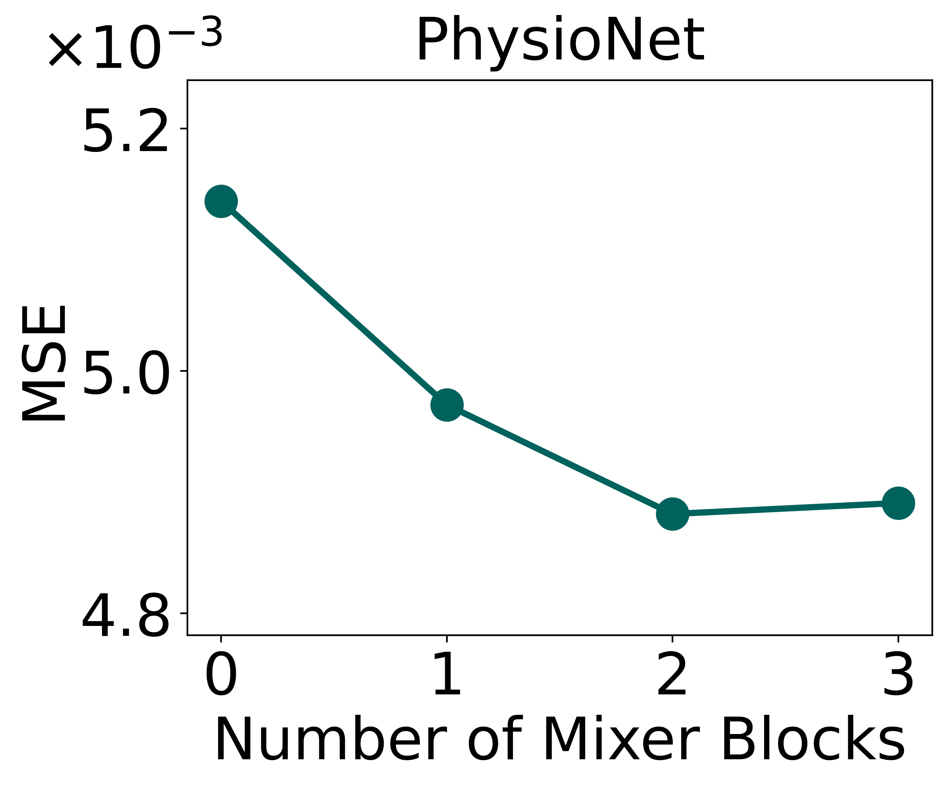
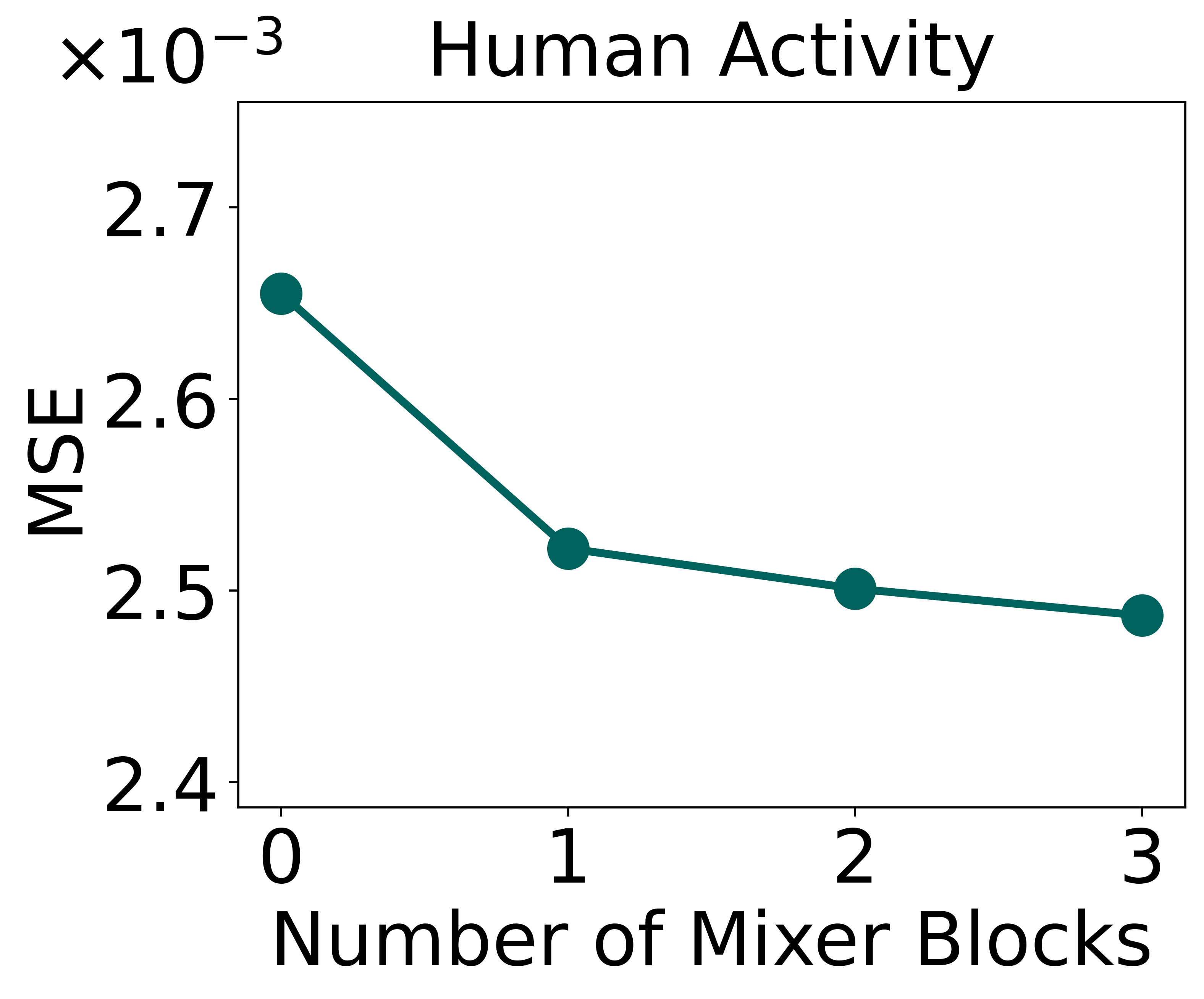
We conducted an experiment to assess the effect of that the number of mixer layers has on the forecasting accuracy on the four PMAU datasets. The results shown in Figure 3 indicate that having at least one mixer block is necessary to obtain the optimal performance. However, stacking more and more mixer blocks is usually not beneficial on the evaluated datasets. Furthermore, we observe that IMTS-Mixer, without a single mixer block, is already competitive with state-of-the-art baselines, showcasing the ability of ISCAM and ConTP.

Figure 3: Test MSE with varying number of mixer blocks.

Table 6: Test MSE on the Physiome-ODE [12] benchmark. The results for the competing models are reported from the Physiome-ODE paper.

	IMTS-	Time-	tPatch-	GraFITi	LinODE-
Dataset	Mixer	CHEAT	GNN		Net	CRU	GraFITi-C
DUP01	0.954±.038	0.978±.030	0.957±.035	0.955±.037	0.964±.036	0.958±.038	0.951±.036
JEL01	0.935±.018	0.966±.027	0.943±.016	0.942±.020	0.949±.015	0.939±.015	0.935±.016
DOK01	0.978±.005	0.997±.004	0.987±.004	0.984±.005	0.996±.003	0.985±.005	0.982±.005
INA01	1.003±.009	1.005±.010	1.004±.009	1.004±.010	1.009±.011	1.005±.010	1.004±.009
WOL01	0.783±.026	0.804±.029	0.795±.027	0.787±.028	0.806±.027	0.814±.029	0.784±.030
BOR01	0.708±.021	0.718±.022	0.719±.019	0.712±.022	0.719±.021	0.715±.020	0.709±.022
HYN01	0.608±.048	0.652±.049	0.630±.045	0.625±.043	0.672±.044	0.665±.053	0.619±.046
JEL02	0.664±.030	0.714±.027	0.702±.023	0.699±.029	0.693±.031	0.674±.028	0.687±.027
DUP02	0.719±.046	0.748±.047	0.728±.049	0.728±.044	0.740±.042	0.722±.046	0.718±.046
WOL02	0.640±.014	0.679±.012	0.656±.016	0.654±.014	0.663±.015	0.653±.017	0.645±.016
DIF01	0.959±.029	0.977±.031	0.991±.027	0.985±.030	0.832±.087	0.985±.025	0.982±.029
VAN01	0.240±.005	0.252±.007	0.247±.007	0.246±.005	0.250±.006	0.253±.005	0.242±.006
DUP03	0.610±.050	0.683±.046	0.624±.052	0.627±.043	0.632±.044	0.622±.047	0.744±.042
BER01	0.277±.013	0.311±.028	0.310±.014	0.300±.018	0.279±.020	0.280±.016	0.342±.018
LEN01	0.547±.043	0.932±.112	0.981±.062	0.607±.055	0.387±.071	0.754±.157	0.970±.063
LI01	0.177±.018	0.438±.019	0.394±.028	0.202±.013	0.084±.009	0.175±.020	0.742±.010
LI02	0.360±.047	0.464±.048	0.438±.048	0.397±.058	0.434±.044	0.437±.046	0.458±.056
REV01	0.603±.045	0.741±.057	0.741±.054	0.674±.055	0.597±.061	0.602±.049	0.855±.050
PUR01	0.143±.017	0.343±.017	0.397±.082	0.153±.006	0.106±.006	0.353±.083	0.476±.020
NYG01	0.237±.051	0.402±.061	0.357±.067	0.344±.065	0.358±.071	0.403±.092	0.366±.047
PUR02	0.251±.022	0.474±.057	0.390±.017	0.322±.021	0.280±.028	0.293±.026	0.511±.023
HOD01	0.383±.052	0.511±.043	0.479±.057	0.493±.046	0.441±.043	0.409±.049	0.609±.056
REE01	0.031±.005	0.044±.007	0.047±.011	0.033±.007	0.045±.012	0.051±.008	0.039±.012
VIL01	0.302±.038	0.385±.045	0.354±.028	0.344±.044	0.374±.021	0.373±.039	0.378±.042
KAR01	0.033±.012	0.050±.013	0.048±.012	0.041±.013	0.034±.008	0.044±.012	0.078±.011
SHO01	0.053±.007	0.085±.019	0.078±.012	0.062±.013	0.057±.006	0.095±.010	0.055±.013
BUT01	0.180±.036	0.306±.079	0.354±.102	0.281±.071	0.254±.074	0.317±.108	0.324±.091
MAL01	0.014±.004	0.044±.002	0.038±.011	0.020±.004	0.018±.007	0.064±.007	0.054±.005
ASL01	0.013±.004	0.029±.003	0.031±.004	0.025±.009	0.022±.003	0.046±.014	0.026±.002
BUT02	0.156±.022	0.272±.031	0.280±.043	0.248±.052	0.207±.056	0.282±.042	0.256±.039
MIT01	0.003±.000	0.003± .000	0.003±.000	0.003±.000	0.003±.000	0.003±.000	0.003±.000
GUP01	0.011±.004	0.060±.014	0.047±.016	0.041±.006	0.018±.007	0.057±.017	0.035±.006
GUY01	0.004±.001	0.015±.004	0.005±.001	0.005±.003	0.006±.005	0.004±.001	0.004±.001
PHI01	0.105±.022	0.308±.019	0.249±.032	0.222±.013	0.131±.014	0.133±.020	0.345±.015
GUY02	0.007±.002	0.032±.006	0.016±.003	0.012±.009	0.010±.006	0.010±.002	0.032±.015
PUL01	0.006±.002	0.036±.011	0.018±.006	0.008±.001	0.008±.004	0.012±.003	0.024±.008
CAL01	0.074±.005	0.720±.357	0.212±.033	0.179±.012	0.078±.009	0.158±.008	0.643±.024
WOD01	0.098±.007	0.372±.293	0.165±.012	0.164±.013	0.154±.016	0.113±.017	0.344±.016
GUP02	0.397±.016	0.445±.018	0.463±.024	0.449±.027	0.469±.022	0.444±.018	0.461±.025
M01	0.003±.000	0.013±.002	0.004±.001	0.003±.000	0.004±.001	0.005±.000	0.003±.000
LEN02	0.031±.005	0.217±.108	0.089±.011	0.099±.021	0.039±.005	0.059±.012	0.143±.022
KAR02	0.143±.007	0.196±.008	0.160±.009	0.151±.009	0.140±.010	0.151±.011	0.252±.010
SHO02	0.021±.003	0.063±.015	0.070±.017	0.043±.006	0.037±.006	0.083±.015	0.073±.010
MAC01	0.016±.002	0.046±.005	0.033±.003	0.021±.003	0.020±.003	0.065±.006	0.019±.002
IRI01	0.027±.005	0.053±.011	0.048±.008	0.038±.017	0.037±.003	0.049±.010	0.097±.008
BAG01	0.026±.002	0.050±.003	0.045±.003	0.029±.002	0.032±.005	0.046±.005	0.109±.002
WOL03	0.062±.009	0.233±.053	0.142±.024	0.105±.016	0.073±.010	0.177±.016	0.247±.032
WAN01	0.082±.007	0.170±.014	0.140±.011	0.119±.010	0.103±.012	0.125±.012	0.232±.015
NEL01	0.006±.001	0.019±.001	0.013±.001	0.007±.000	0.010±.001	0.009±.001	0.023±.006
HUA01	0.037±.001	0.099±.006	0.090±.012	0.063±.005	0.052±.004	0.116±.007	0.115±.007

Table 7: Exact number of trainable parameters on each Physiome-ODE dataset.

Dataset	IMTS-Mixer	TimeCHEAT	tPatchGNN	GraFITi
DUP01	173,075	1,279,382	365,594	315,329
JEL01	39,053	1,279,382	390,170	236,673
DOK01	105,219	338,203	159,610	1,255,297
INA01	139,891	337,282	159,830	15,825
WOL01	95,195	344,723	390,310	315,777
BOR01	178,201	341,702	365,614	1,253,377
HYN01	315,631	339,608	365,994	1,255,809
JEL02	17,741	645,014	365,594	627,329
DUP02	42,317	341,702	165,454	627,457
WOL02	192,745	343,695	160,414	315,649
DIF01	52,321	659,850	159,570	1,255,041
VAN01	80,459	642,011	390,330	1,254,273
DUP03	56,083	653,849	365,594	158,017
BER01	95,625	641,920	365,774	1,254,401
LEN01	42,317	646,214	365,614	315,393
LI01	65,179	343,376	365,654	315,521
LI02	48,095	343,376	365,654	1,253,633
REV01	44,699	1,282,256	390,230	1,253,633
PUR01	59,109	341,702	165,454	315,393
NYG01	139,891	343,747	165,974	1,256,705
PUR02	65,165	646,214	165,454	1,253,377
HOD01	62,141	342,531	390,210	1,253,505
REE01	39,997	655,491	365,634	315,457
VIL01	236,175	334,849	165,574	315,777
KAR01	130,321	644,156	390,450	1,255,041
SHO01	700,145	679,820	166,514	1,260,161
BUT01	61,353	342,531	390,210	1,253,505
MAL01	236,725	344,336	165,574	315,777
ASL01	143,079	651,229	390,730	1,256,833
BUT02	62,141	342,531	390,210	1,253,505
MIT01	192,745	344,082	165,534	236,993
GUP01	39,997	332,915	165,474	1,253,505
GUY01	168,461	340,631	165,434	5,249
PHI01	199,845	1,280,582	159,310	1,253,377
GUY02	168,461	653,462	390,170	236,673
PUL01	168,461	653,462	159,290	158,017
CAL01	284,951	1,282,977	390,470	1,255,169
WOD01	56,473	638,710	165,454	1,253,377
GUP02	45,205	655,491	159,330	1,253,505
M01	193,811	340,502	365,594	158,017
LEN02	176,997	638,710	159,310	1,253,377
KAR02	115,255	335,936	390,390	1,254,657
SHO02	528,233	672,187	166,514	1,260,161
MAC01	52,913	343,953	390,270	315,649
IRI01	97,937	654,482	390,590	316,673
BAG01	85,813	657,425	365,734	628,225
WOL03	275,821	658,641	365,814	1,254,657
WAN01	44,699	640,642	159,350	1,253,633
NEL01	62,141	342,789	365,634	1,253,505
HUA01	130,093	348,077	365,914	1,255,297

Table 8: Inference time in seconds of each model on the datasets contained in the Physiome-ODE benchmark.

Dataset	IMTS-Mixer	TimeCHEAT	tPatchGNN	GraFITi
DUP01	0.064	2.772	0.088	1.508
JEL01	0.061	2.704	0.125	1.419
DOK01	0.078	2.377	0.117	1.596
INA01	0.087	2.511	0.136	1.503
WOL01	0.063	2.461	0.153	1.517
BOR01	0.059	2.509	0.095	1.504
HYN01	0.092	2.526	0.154	1.601
JEL02	0.058	2.617	0.090	1.343
DUP02	0.053	2.398	0.113	1.342
WOL02	0.066	2.520	0.110	1.482
DIF01	0.071	2.623	0.107	1.592
VAN01	0.063	2.360	0.148	1.404
DUP03	0.056	2.316	0.089	1.201
BER01	0.065	2.450	0.128	1.473
LEN01	0.054	2.555	0.093	1.482
LI01	0.064	2.383	0.103	1.504
LI02	0.058	2.484	0.100	1.514
REV01	0.061	2.708	0.129	1.505
PUR01	0.060	2.530	0.122	1.531
NYG01	0.097	2.479	0.222	1.598
PUR02	0.054	2.575	0.101	1.500
HOD01	0.061	2.500	0.129	1.530
REE01	0.062	2.640	0.096	1.505
VIL01	0.070	2.375	0.164	1.508
KAR01	0.073	2.484	0.224	1.536
SHO01	0.115	2.724	0.359	1.604
BUT01	0.058	2.376	0.117	1.493
MAL01	0.066	2.445	0.146	1.484
ASL01	0.076	2.313	0.300	1.387
BUT02	0.062	2.523	0.122	1.506
MIT01	0.062	2.344	0.126	1.290
GUP01	0.056	2.284	0.118	1.390
GUY01	0.063	2.432	0.116	1.265
PHI01	0.061	2.808	0.091	1.509
GUY02	0.060	2.599	0.121	1.442
PUL01	0.060	2.576	0.089	1.356
CAL01	0.075	2.537	0.213	1.462
WOD01	0.059	2.581	0.107	1.527
GUP02	0.055	2.644	0.089	1.502
M01	0.064	2.538	0.098	1.364
LEN02	0.061	2.566	0.095	1.523
KAR02	0.065	2.479	0.242	1.503
SHO02	0.141	3.060	0.286	1.711
MAC01	0.061	2.379	0.161	1.510
IRI01	0.072	2.504	0.197	1.482
BAG01	0.057	2.368	0.113	1.260
WOL03	0.068	2.498	0.137	1.483
WAN01	0.063	2.521	0.100	1.501
NEL01	0.056	2.315	0.093	1.366
HUA01	0.075	2.514	0.137	1.568

References

- [1] (2021) Neural Flows: Efficient Alternative to Neural ODEs. In NeurIPS, Cited by: Appendix 0.A, Appendix 0.C, Appendix 0.C, §2.2, §6.
- [2] (2018-04) Recurrent Neural Networks for Multivariate Time Series with Missing Values. Scientific Reports 8 (1), pp. 6085. External Links: ISSN 2045-2322, Document Cited by: §6.
- [3] (2018) Neural Ordinary Differential Equations. In NeurIPS, Cited by: §2.2.
- [4] (2023-04-24) TSMixer: An All-MLP Architecture for Time Series Forecasting. TMLR. External Links: ISSN 2835-8856 Cited by: Appendix 0.B, §1, §2.1, §3, §5.3, §6.
- [5] (2019) GRU-ODE-Bayes: Continuous Modeling of Sporadically-Observed Time Series. In NeurIPS, Cited by: Appendix 0.A, §1, §2.2.
- [6] (2024) The Road Less Scheduled. arXiv. External Links: Document Cited by: Appendix 0.B, §6.
- [7] (2020) An Image is Worth 16x16 Words: Transformers for Image Recognition at Scale. In ICLR, Cited by: §3.
- [8] (2023-08-04) TSMixer: Lightweight MLP-Mixer Model for Multivariate Time Series Forecasting. KDD. Cited by: §1, §2.1.
- [9] (2020-11) Set Functions for Time Series. In Proceedings of the 37th International Conference on Machine Learning, pp. 4353–4363. External Links: ISSN 2640-3498 Cited by: §5.1.
- [10] (2016-05) MIMIC-III, a freely accessible critical care database. Scientific Data 3 (1), pp. 160035. External Links: ISSN 2052-4463, Document Cited by: Appendix 0.A, §6.
- [11] (2017-01) Adam: A Method for Stochastic Optimization. arXiv. External Links: 1412.6980, Document Cited by: Appendix 0.B, §6.
- [12] (2024-10) Physiome-ODE: A Benchmark for Irregularly Sampled Multivariate Time-Series Forecasting Based on Biological ODEs. In The Thirteenth International Conference on Learning Representations, Cited by: Appendix 0.B, Appendix 0.B, Appendix 0.C, Appendix 0.C, Table 6.
- [13] (2025) Timecheat: A channel harmony strategy for irregularly sampled multivariate time series analysis. In Proceedings of the AAAI Conference on Artificial Intelligence, Vol. 39, pp. 18861–18869. Cited by: Appendix 0.B, Appendix 0.C, Appendix 0.D, §1, §2.2, §6, §6.
- [14] (2023-10) iTransformer: Inverted Transformers Are Effective for Time Series Forecasting. In The Twelfth International Conference on Learning Representations, Cited by: §2.1.
- [15] (2019-01) Decoupled Weight Decay Regularization. arXiv. External Links: 1711.05101, Document Cited by: Appendix 0.B, §6.
- [16] (2006-01) U.S. HISTORICAL CLIMATOLOGY NETWORK (USHCN): Daily Temperature, Precipitation and Snow Data. Technical report Environmental System Science Data Infrastructure for a Virtual Ecosystem (ESS-DIVE) (United States). External Links: Document Cited by: Appendix 0.A, §6.
- [17] (2022-09) A Time Series is Worth 64 Words: Long-term Forecasting with Transformers. In The Eleventh International Conference on Learning Representations, Cited by: §2.1, §6.
- [18] (2019) Latent Ordinary Differential Equations for Irregularly-Sampled Time Series. In NeurIPS, Cited by: §1, §2.2, §6.
- [19] (2022-06) Modeling Irregular Time Series with Continuous Recurrent Units. In Proceedings of the 39th International Conference on Machine Learning, pp. 19388–19405. External Links: ISSN 2640-3498 Cited by: Appendix 0.A, Appendix 0.C, Appendix 0.C, §1, §2.2, §6.
- [20] (2022-09) Latent Linear ODEs with Neural Kalman Filtering for Irregular Time Series Forecasting. Cited by: Appendix 0.C, Appendix 0.C.
- [21] (2020-10) Multi-Time Attention Networks for Irregularly Sampled Time Series. In International Conference on Learning Representations, Cited by: §6.
- [22] (2012-09) Predicting in-hospital mortality of ICU patients: The PhysioNet/Computing in cardiology challenge 2012. In 2012 Computing in Cardiology, pp. 245–248. External Links: ISSN 2325-8853 Cited by: Appendix 0.A, §6.
- [23] (2021) MLP-Mixer: An all-MLP Architecture for Vision. In NeurIPS, Cited by: §1, §2.1, §3.
- [24] (2017) Attention is All you Need. In NeurIPS, Vol. 30. Cited by: Appendix 0.D, §2.1, §5.1.
- [25] (2010) Localization Data for Person Activity. UCI Machine Learning Repository. External Links: Document Cited by: Appendix 0.A, §6.
- [26] (2022-09) TimesNet: Temporal 2D-Variation Modeling for General Time Series Analysis. In The Eleventh International Conference on Learning Representations, Cited by: §6.
- [27] (2021) Autoformer: Decomposition Transformers with Auto-Correlation for Long-Term Series Forecasting. In NeurIPS, Cited by: §2.1.
- [28] (2023) Tripletformer for Probabilistic Interpolation of Irregularly sampled Time Series. In BigData, External Links: Document Cited by: §5.1.
- [29] (2024) GraFITi: Graphs for Forecasting Irregularly Sampled Time Series. Proceedings of the AAAI Conference on Artificial Intelligence. External Links: ISSN 2374-3468, Document Cited by: Appendix 0.A, Appendix 0.B, Appendix 0.C, Appendix 0.D, §1, §2.2, §2.2, §5.1, Table 1, §6.
- [30] (2025-04) Probabilistic Forecasting of Irregularly Sampled Time Series with Missing Values via Conditional Normalizing Flows. Proceedings of the AAAI Conference on Artificial Intelligence 39 (20), pp. 21877–21885. External Links: ISSN 2374-3468 Cited by: §8.
- [31] (2026) Reliable Probabilistic Forecasting of Irregular Time Series through Marginalization-Consistent Flows. In ICLR, Cited by: §8.
- [32] (2023-06) Are Transformers Effective for Time Series Forecasting?. Proceedings of the AAAI Conference on Artificial Intelligence 37 (9), pp. 11121–11128. External Links: ISSN 2374-3468, Document Cited by: §2.1, §6.
- [33] (2019) Root Mean Square Layer Normalization. In NeurIPS, Vol. 32. Cited by: item 2, §5.2.
- [34] (2024-06) Irregular Multivariate Time Series Forecasting: A Transformable Patching Graph Neural Networks Approach. In Forty-First International Conference on Machine Learning, Cited by: Appendix 0.B, Appendix 0.C, Appendix 0.D, §1, §2.2, §2.2, §5.1, Table 1, §6, §6.
- [35] (2024-08) Irregular Traffic Time Series Forecasting Based on Asynchronous Spatio-Temporal Graph Convolutional Networks. In KDD, pp. 4302–4313. Cited by: Appendix 0.D, §5.1.
- [36] (2022-09) Crossformer: Transformer Utilizing Cross-Dimension Dependency for Multivariate Time Series Forecasting. In The Eleventh International Conference on Learning Representations, Cited by: §6.
- [37] (2021-05) Informer: Beyond Efficient Transformer for Long Sequence Time-Series Forecasting. Proceedings of the AAAI Conference on Artificial Intelligence 35 (12), pp. 11106–11115. External Links: ISSN 2374-3468, Document Cited by: §2.1.
- [38] (2022-06) FEDformer: Frequency Enhanced Decomposed Transformer for Long-term Series Forecasting. In Proceedings of the 39th International Conference on Machine Learning, pp. 27268–27286. External Links: ISSN 2640-3498 Cited by: §2.1.