Model-Adaptive Approach to Dynamic Discrete Choice Models with Large State Spaces

Estimation and counterfactual experiments in dynamic discrete choice models with large state spaces pose computational difficulties. This paper proposes a model-adaptive approach, based on the conjugate gradient (CG) method, to solve the linear system of fixed point equations of the policy valuation operator. We propose a model-adaptive sieve space, constructed by iteratively augmenting the space with the residual from the previous iteration. We show both theoretically and numerically that model-adaptive sieves dramatically improve performance. In particular, the approximation error decays at a superlinear rate in the sieve dimension, unlike a linear rate achieved using successive approximation. Our method works for both conditional choice probability estimators and full-solution estimators with policy iteration or Newton–Kantorovich iterations. We apply the method to analyze consumer demand for laundry detergent using Kantar’s Worldpanel Take Home data. On average, our method is 80% faster than successive approximation and the exact equation solver in solving the dynamic programming problem, substantially reducing the computational cost of the Bayesian MCMC estimator.
Keywords: Dynamic discrete choice; Adaptive sieve; Policy iteration; Demand for storable goods.
JEL codes: C61, C63, C25, L66.

1 Introduction

Dynamic Discrete Choice (DDC) models with large state spaces have become increasingly popular due to their ability to capture decision-making processes in complex high-dimensional settings. However, estimation and counterfactual experiments in these settings pose significant computational challenges. This paper proposes a model-adaptive approach, based on the conjugate gradient (CG) method, to solve the linear system of fixed point equations of the policy valuation operator. Our goal is to provide a fast and easily implementable method to solve the equations within a pre-specified tolerance. As the policy valuation step is fundamental to Conditional Choice Probability (CCP) estimators, full-solution estimators and counterfactual experiments with policy iteration or Newton–Kantorovich iterations, our approach offers a useful numerical tool across various empirical applications, expanding the set of complex high-dimensional settings in which DDC models can be used.

The policy valuation operator, as described in Aguirregabiria and Mira (2002), involves solving for the value function implied by an arbitrary policy function, which may not necessarily be optimal. This value function represents the expected discounted utility if an individual behaves according to that policy function. CCP estimators (e.g., Hotz and Miller (1993), Aguirregabiria and Mira (2002, 2007), Pesendorfer and Schmidt-Dengler (2008), and Arcidiacono and Miller (2011)) use the policy valuation operator to solve for the value function given a consistent estimator of CCPs. If policy iteration or Newton–Kantorovich iterations are used for full solution estimators or counterfactual experiments, each iteration employs the policy valuation operator. However, in models with large state spaces, policy valuation remains computationally demanding and requires efficient numerical methods. The accuracy of these methods is crucial for obtaining reliable estimates. Dubé et al. (2012) shows that loose tolerance thresholds can lead to bias in parameter estimates. Therefore, there is a clear need for fast and accurate numerical methods for DDC models with large state spaces.

This paper proposes a model-adaptive (MA) approach to solve the linear system of fixed point equations of the policy valuation operator. The primary goal is to achieve a pre-specified tolerance while significantly reducing computational costs, enabling the use of policy valuation tools in a wide range of empirical applications. We call our approach model-adaptive as it designs the sieve space based on the model primitives (such as the transition density and utility function), and the algorithm itself selects the sieve dimension. At each step, our approach augments the sieve space with the residual from the previous iteration and projects the value function onto the augmented sieve space. It achieves a faster decay rate of the approximation error than conventional methods, such as Successive Approximation (SA), which iterates the contraction mapping, and Temporal Difference (TD), which projects the value function onto a pre-specified sieve space. Formally, we show that the approximation error decays at a superlinear rate in the sieve dimension (number of iterations), while SA achieves a linear rate and TD achieves only a sublinear rate. Furthermore, the sieve space and its dimension are automatically constructed by the algorithm, eliminating the need for researchers to design the sieve space and choose its dimension. Consequently, our method is easy to implement and converges faster than conventional methods, offering substantial computational savings.

The main computational cost depends on the number of iterations and matrix-vector multiplication operations. Our approach attains superlinear convergence on the approximation error, which substantially reduces the number of iterations required to reach a desired level of tolerance. Formally, our approach achieves an approximation error upper bound of $O((\frac{C_{1}}{\sqrt{k}})^{k})$, where $k$ is the number of iterations and $C_{1}$ is a constant. Furthermore, the bound can be improved to $O((\frac{C_{2}}{k})^{k})$ if the transition density has continuous partial derivatives. Notably, only the constants in the upper bound depend on the discount factor and properties of the transition density (such as its boundedness and smoothness). Unlike SA, whose convergence rate is governed by the contraction modulus $\beta$ and slows significantly as $\beta\to 1$, our method’s superlinear convergence does not rely on the contraction property. Therefore, our method is well-suited for models with large state spaces and large discount factors, such as dynamic consumer demand models (e.g., Hendel and Nevo (2006) and Wang (2015)). Moreover, it works particularly well for models with smooth transition densities, such as autoregressive (AR) processes, which are commonly used in empirical applications (e.g., Sweeting (2013), Huang and Smith (2014), Kalouptsidi (2014), Grieco et al. (2022), and Gerarden (2023)).

We provide implementations for both discrete and continuous state spaces. For discrete state spaces, the implementation requires only matrix operations as the system of equations takes the form of a finite-dimensional linear system. For continuous state spaces, we employ numerical integration to approximate the integral of the policy valuation step. Thus, there is a trade-off between simulation error and computational cost: increasing the number of grid points reduces simulation error at the cost of solving a larger linear system within a given tolerance. The computational cost of matrix-vector multiplication operations increases with the number of grid points. Therefore, we analyze the impact of the number of grid points on the number of iterations required to achieve a desired tolerance. We show that the number of iterations required for convergence remains approximately the same for all sufficiently large numbers of grid points. As a result, we can expect the number of iterations to be independent of the number of grid points for numerical integration. Therefore, our method allows researchers to reduce simulation error by increasing the number of grid points up to the computational limits of matrix-vector multiplication. Fast matrix-vector multiplication algorithms can further accelerate the computation (e.g., Rokhlin (1985), Greengard and Rokhlin (1987), and Hackbusch and Nowak (1989)). In addition, matrix-vector multiplication is amenable to GPU acceleration, which can further reduce the computational cost.

We illustrate the performance of our approach using three numerical experiments. We first simulate the bus engine replacement problem to visualize the convergence behavior of our method. The plot of our approximation solution shows that the method uses a few iterations to find a good sieve space. After that, it converges rapidly to the true solution.

Second, we analyze a model for dynamic consumer demand for storable goods similar to Hendel and Nevo (2006). We compare policy iteration and Newton–Kantorovich outer iterations combined with different inner solvers (MA, SA, and an exact solver), along with VFI benchmarks. We demonstrate that PI+MA is 80% faster than conventional methods such as SA and an exact equation solver. It is also more than 90 times faster than one-step value function iteration methods. These substantial computational savings open the door to the use of Bayesian MCMC estimators (Chernozhukov and Hong (2003)), which are well-suited as the likelihood function is not differentiable in utility parameters.

Third, we examine a dynamic firm entry and exit problem in Aguirregabiria and Magesan (2023). We solve the dynamic programming problem by policy iteration using MA to solve the linear system of fixed point equations. We vary the discount factor and number of grid points for numerical integration to evaluate the performance. The computational times confirm that our method improves the computational efficiency of policy iteration. The results show that the numbers of iterations required for convergence are approximately the same regardless of the numbers of grid points. Moreover, the number of iterations only slightly increases as the discount factor approaches one. Finally, we compare our method with TD and SA. The simulation results show that our method outperforms SA in terms of computational time and TD in terms of approximation error.

We apply our method to a dynamic consumer demand model for laundry detergent using Kantar’s Worldpanel Take Home data. For each household size, we separately estimate the dynamic parameters using the Bayesian MCMC estimator. At each MCMC step, we solve the dynamic programming problem by policy iteration with MA. The results confirm the computational efficiency of our method in practice. We also simulate the long-run elasticities, which reveal the heterogeneous substitution patterns across different household sizes.

1.1 Related Literature

Sieve approximation methods have been used to solve dynamic programming problems (e.g., Norets (2012), Arcidiacono et al. (2013), and Wang (2015)). They have been widely used to solve the linear equations in the policy valuation step. Applications include Hendel and Nevo (2006), Sweeting (2013), and Bodéré (2023). Recent work approximates the solution to the linear equation by temporal difference (see Adusumilli and Eckardt (2025)). However, those methods require researchers both to design the space of basis functions (e.g., polynomials, splines, or neural networks) and choose the sieve dimension (e.g., the degree of polynomials, the number of knots, and the number of hidden layers). The best choice for each application is almost always unclear. In contrast, MA constructs a model-adaptive sieve space using the algorithm itself to design that space. The sieve dimension (i.e., the number of iterations) is also determined by the algorithm. The method is guaranteed to achieve the pre-specified tolerance. Finally, we show that the approximation error decays at a superlinear rate in the sieve dimension. Other methods like TD achieve only a sublinear rate.

Successive Approximation (see Kress (2014)), also known as fixed point iteration (Judd (1998)), is an iterative method to solve the fixed point equations of the policy valuation operator. The computational cost depends on the number of iterations and the number of matrix-vector multiplication operations. The convergence of SA relies on the $\beta$-contraction property of the transition operator $\mathcal{T}$, where $\beta$ is the discount factor. Therefore, the number of iterations of SA increases significantly as the discount factor approaches one, making the methods computationally demanding. In contrast, the superlinear convergence of our method does not rely on the contraction property, making it particularly well-suited for models with large discount factors such as consumer demand models (e.g., Hendel and Nevo (2006) and Wang (2015)). Moreover, our method can outperform SA even for small discount factors as SA achieves linear convergence while our method achieves superlinear convergence.

For continuous state spaces, we employ numerical integration to approximate the integral of the policy valuation operator, which implicitly discretizes the state space. Discretization is widely used in economics (e.g., Sweeting (2013), Kalouptsidi (2014), Huang et al. (2015), and Bodéré (2023)). Rust (1997b, a) study the simulation error from numerical integration and assume the discretized equation can be solved exactly. However, there is a trade-off between simulation error and computational cost of solving the discretized equation. Increasing the number of grid points reduces the simulation error while increasing the size of the linear system to be solved; potentially making it computationally infeasible to solve the system exactly. Sieve approximation is used to solve the discretized equation (e.g., Hendel and Nevo (2006), Sweeting (2013), and Bodéré (2023)). Instead, we propose to solve the discretized equation within a given tolerance while minimizing computational cost. The computational cost of MA depends on the number of iterations and the number of matrix-vector multiplication operations. We can expect that the number of iterations is small and independent of the number of grid points. Therefore, MA enables researchers to reduce simulation error up to the computational limits of matrix-vector multiplication.

Outline: The remainder of the paper is organized as follows. Section 2 reviews DDC models and the policy valuation operator. Section 3 presents the model-adaptive approach, its implementation and computational cost. Section 4 describes the theoretical properties. Section 5 reports results from three numerical experiments. Section 6 applies our method to a consumer demand for storable goods. Section 7 concludes. The proofs are in Appendix A. Appendix B contains details of algorithms of simulations and empirical application.

Notation: Let $\mathbb{X}$ be the support of $x$, and $\mathbb{A}:=\{0,1,\cdots,A-1\}$. $\mathbb{X}$ can be discrete or continuous. For a probability distribution $\mu$ on $\mathbb{X}$, which in the continuous case is assumed to be absolutely continuous with respect to Lebesgue measure, let $L^{2}(\mathbb{X},\mu)$ denote the space of square-integrable functions on $\mathbb{X}$. Let $\langle\cdot,\cdot\rangle_{\mu}$ and $\|\cdot\|_{\mu}$ denote the inner product and norm induced by $\mu$. Let $\nu_{Leb}$ denote the Lebesgue measure, and let $\langle\cdot,\cdot\rangle$, $\|\cdot\|$, and $L^{2}(\mathbb{X})$ denote the inner product, norm, and $L^{2}$-space, respectively. We suppress $\nu_{Leb}$ for notational simplicity. Let $\|\cdot\|_{\infty}$ denote the sup-norm of a vector. For a linear operator, $\mathcal{A}:L^{2}(\mathbb{X})\longmapsto L^{2}(\mathbb{X})$, denote by $\|\mathcal{A}\|_{op}:=\sup_{h\in L^{2}(\mathbb{X}),\|h\|=1}\|\mathcal{A}h\|$ the operator norm. Let $\mathcal{I}$ be the identity operator.

2 Model

2.1 Framework

We study infinite horizon stationary dynamic discrete choice models as in Rust (1994). In each discrete period $t=0,1,2,\ldots$, an individual chooses $a_{t}\in\mathbb{A}$ to maximize her discounted expected utility:

$$\mathbb{E}\left[\sum_{t=0}^{\infty}\beta^{t}\left[u(x_{t},a_{t})+\varepsilon_{t}(a_{t})\right]\bigg|x_{0},\varepsilon_{0}\right]$$

where $\beta\in(0,1)$ is the discount factor, $u(x_{t},a_{t})$ is the period utility, $x_{t}\in\mathbb{X}$ is the observable state (to researchers) that follows a first-order Markov process with a transition density $f(x_{t+1}|x_{t},a_{t})$, $\varepsilon_{t}\in\mathbb{R}^{A}$ is a vector of unobservable i.i.d. type I extreme value shocks with Lebesgue density $g(\varepsilon_{t})$, and $\varepsilon_{t}(a_{t})$ is the element of $\varepsilon_{t}$ corresponding to $a_{t}$.

Under regularity conditions (see Rust (1994)), the utility maximization problem has a solution and the optimal value function $V_{opt}(x,\varepsilon)$ is the unique solution to the Bellman equation:

$$V_{opt}(x,\varepsilon)=\max_{a\in\mathbb{A}}\biggl\{u(x,a)+\varepsilon(a)+\beta\int V_{opt}(x^{\prime},\varepsilon^{\prime})f(x^{\prime}|x,a)g(\varepsilon^{\prime})dx^{\prime}d\varepsilon^{\prime}\biggr\}$$

where $(x^{\prime},\varepsilon^{\prime})$ denotes the next period’s state and utility shock. Under the i.i.d. assumption on utility shocks, integrating the utility shocks out, the integrated Bellman equation has the following form:

$$V_{opt}(x)=\int\max_{a\in\mathbb{A}}\biggl\{v^{*}(x,a)+\varepsilon(a)\biggr\}g(\varepsilon)d\varepsilon$$

where $V_{opt}(x)$ is the integrated value function and $v^{*}(x,a)$ is the conditional value function defined as:

$$v^{*}(x,a):=u(x,a)+\beta\int V_{opt}(x^{\prime})f(x^{\prime}|x,a)dx^{\prime}$$

The conditional choice probability (CCP) is the probability that action $a$ is optimal conditional on observable state $x$ defined by:

$$p^{*}(a|x):=\int\mathbbm{1}\left\{a=\operatornamewithlimits{argmax}_{a\in\mathbb{A}}\{v^{*}(x,a)+\varepsilon(a)\}\right\}g(\varepsilon)d\varepsilon$$

where $\mathbbm{1}\{\cdot\}$ is the indicator function. Under the distributional assumption on utility shocks, CCPs take the following form:

$$p^{*}(a|x)=\frac{\exp(v^{*}(x,a))}{\sum_{a}\exp(v^{*}(x,a))}$$

The following map is derived in Arcidiacono and Miller (2011) as a corollary of Hotz–Miller Inversion Lemma by Hotz and Miller (1993), $\forall\ (x,a)\in\mathbb{X}\times\mathbb{A}$:

$$V_{opt}(x)=v^{*}(x,a)-\log p^{*}(a|x)+\kappa$$ (2.1)

where $\kappa$ is the Euler constant. The equation (2.1) establishes a crucial link between the integrated value function $V_{opt}(x)$, conditional value function $v^{*}(x,a)$, and conditional choice probabilities $p^{*}(a|x)$. It provides a powerful tool for the policy valuation step, which is essential for both policy iteration and CCP estimators.

2.2 Policy Valuation Operator

The policy valuation operator (see Aguirregabiria and Mira (2002)) maps an arbitrary policy function to the value function using (2.1). The value function represents the expected discounted utility of an individual if she behaves today and in the future according to that policy, which is not necessarily optimal. Aguirregabiria and Mira (2002) shows that the value function is obtained by solving the following equation for $V$ given a policy function $p$:

$$V(x)=\sum_{a}p(a|x)\left[u(x,a)+\kappa-\log p(a|x)+\beta\mathbb{E}_{x^{\prime}|x,a}V(x^{\prime})\right]$$ (2.2)

In this paper, we focus on solving (2.2) for a given policy function. Therefore, we introduce the following notations and suppress the dependence on $p$:

Definition 1.

For a given policy function $p$, define:

1. $f(x^{\prime}|x):=\sum_{a}p(a|x)f(x^{\prime}|x,a)$ and $\mathcal{T}V(x):=\beta\int f(x^{\prime}|x)V(x^{\prime})dx^{\prime}$.

2. $u(x)=\sum_{a}p(a|x)u(x,a)+\kappa-\sum_{a}p(a|x)\log p(a|x)$.

Using this notation, we can rewrite (2.2) as a linear system of fixed point equations:

$$(\mathcal{I}-\mathcal{T})V=u$$ (2.3)

Both CCP estimators and the policy iteration method (see Howard (1960)) require solving equation (2.3) for $V$. For CCP estimators, $p$ is replaced with its consistent estimator $\hat{p}$. For policy iteration, at iteration $i$, we solve for $V_{i}$ associated with $p_{i}$ from the previous iteration. Subsequently, the policy improvement step updates the policy function as follows:

$$p_{i+1}(a|x)=\frac{\exp(v_{i}(x,a))}{\sum_{a}\exp(v_{i}(x,a))}$$

where $v_{i}(x,a)=u(x,a)+\beta\mathbb{E}_{x^{\prime}|x,a}V_{i}(x^{\prime})$. This process iterates until convergence of the policy function is achieved.

2.3 Newton–Kantorovich Iterations

An alternative full-solution method is the Newton–Kantorovich (NK) iteration applied to the integrated Bellman equation, as considered in Rust (1987). Define the Bellman operator $\Gamma:\mathbb{R}^{|\mathbb{X}|}\to\mathbb{R}^{|\mathbb{X}|}$ by:

$$\Gamma(V)(x):=\log\sum_{a\in\mathbb{A}}\exp\left(u(x,a)+\beta\mathbb{E}_{x^{\prime}|x,a}V(x^{\prime})\right)+\kappa$$

The fixed point of $\Gamma$ is the integrated value function $V_{opt}$. The Jacobian of $\Gamma$ at $V_{k}$ is the matrix $\mathcal{T}_{k}$ with entries:

$$\mathcal{T}_{k}(x,x^{\prime}):=\beta\sum_{a\in\mathbb{A}}p_{k}(a|x)f(x^{\prime}|x,a)$$

where $p_{k}(a|x):=\frac{\exp(v_{k}(x,a))}{\sum_{a^{\prime}}\exp(v_{k}(x,a^{\prime}))}$ is the CCP induced by $V_{k}$. The NK step is:

$$(\mathcal{I}-\mathcal{T}_{k})d_{k}=\Gamma(V_{k})-V_{k},\qquad V_{k+1}=V_{k}+d_{k}$$ (2.4)

Note that $\mathcal{T}_{k}$ has the same structure as $\mathcal{T}$ in (2.3). In addition, the NK step coincides with the policy iteration step under the i.i.d. extreme value assumption. Therefore, (2.4) is a linear system of the form $(\mathcal{I}-\mathcal{T})V=u$, where the operator $\mathcal{T}_{k}$ and right-hand side $\Gamma(V_{k})-V_{k}$ change at each NK iteration. The MA approach developed in the next section applies directly to solving (2.4). While NK iterations enjoy quadratic convergence to the fixed point of $\Gamma$ (see Rust (1988)), each NK step requires solving the linear system (2.4), which becomes computationally demanding for large state spaces. Our method provides an efficient solver for this inner linear system.

Remark 1.

Throughout this paper, we distinguish two levels of convergence. The outer convergence refers to the PI or NK iterations converging to the fixed point of the Bellman operator. The inner convergence refers to the MA iterations solving the linear system at each outer step. The superlinear convergence results in this paper concern the inner MA iterations, not the outer PI or NK convergence.

3 Model-Adaptive Approach

This section presents the model-adaptive (MA) approach, its implementation and computational cost. Our method employs the Conjugate Gradient (CG) method, an iterative approach for solving large linear systems. The CG method is commonly attributed to Hestenes et al. (1952). For comprehensive textbooks, see Kelley (1995) and Han and Atkinson (2009).

The CG was originally designed for solving linear systems with self-adjoint operators. However, the operator $\mathcal{T}$ is not necessarily self-adjoint. If $\mathcal{T}$ were self-adjoint with respect to the inner product space $\langle\cdot,\cdot\rangle_{\mu}$, then the Markov chain would be time-reversible, which is a strong assumption in many practical settings. Therefore, instead of solving (2.3) for $V$ directly, we propose to solve the following equation for $y$:

$$(\mathcal{I}-\mathcal{T})(\mathcal{I}-\mathcal{T}^{*})y=u$$ (3.1)

and set $V=(\mathcal{I}-\mathcal{T}^{*})y$ to solve (2.3), where $\mathcal{T}^{*}$ is the adjoint operator of $\mathcal{T}$.

For discrete state spaces, (3.1) boils down to a finite-dimensional linear system. For continuous state spaces, we will use deterministic numerical integration to approximate the integral in (3.1).

The adjoint operator $\mathcal{T}^{*}$ is defined with respect to an inner product space. The choice of the inner product does affect the convergence rate of the approximation error. Nevertheless, approximation solutions on different spaces all converge superlinearly under regularity conditions. To achieve the fastest decay of the approximation error when using CG, we propose to solve (3.1) on $L^{2}(\mathbb{X})$ and define $\mathcal{T}^{*}$ by the inner product $\langle\cdot,\cdot\rangle$. Lemma 7 formally discusses the convergence rate. Theorem 1(i) shows the existence and uniqueness of the solution to (3.1) on $L^{2}(\mathbb{X})$, denoted by $y^{*}$. Moreover, Theorem 1(ii) proves $V^{*}=(\mathcal{I}-\mathcal{T}^{*})y^{*}$ where $V^{*}$ is the solution to (2.3) on $L^{2}(\mathbb{X},\mu)$.

The key idea of the conjugate gradient method is to iteratively build a solution by searching along directions that are conjugate (i.e., orthogonal with respect to the operator $(\mathcal{I}-\mathcal{T})(\mathcal{I}-\mathcal{T}^{*})$). At each iteration, the algorithm: (i) chooses a step size $\alpha_{k-1}$ that minimizes the residual along the current search direction $s_{k-1}$; (ii) computes the new residual $r_{k}$; and (iii) constructs the next search direction $s_{k}$ by combining the new residual with the previous direction, where the coefficient $\beta_{k-1}$ ensures conjugacy. The residuals $r_{0},r_{1},\ldots$ are mutually orthogonal by construction, and they form the basis of the model-adaptive sieve space. The model-adaptive approach is as follows:

Algorithm 1 (Model-adaptive Approach).

Input: Operator $\mathcal{T}$, adjoint $\mathcal{T}^{*}$ where $\mathcal{T}^{*}V(x)=\beta\int V(x^{\prime})f(x|x^{\prime})dx^{\prime}$, right-hand side $u$, tolerance $tol$.

Initialize: $y_{0}=0$, $r_{0}=s_{0}=u$.

For $k=1,2,\ldots$ until $\|r_{k}\|\leq tol$:

$$\begin{array}[]{ll}\text{Step 1:}\quad y_{k}=y_{k-1}+\alpha_{k-1}s_{k-1}&\alpha_{k-1}=\frac{\left\|r_{k-1}\right\|^{2}}{\|(\mathcal{I}-\mathcal{T}^{*})s_{k-1}\|^{2}}\\[6.0pt] \text{Step 2:}\quad r_{k}=u-(\mathcal{I}-\mathcal{T})(\mathcal{I}-\mathcal{T}^{*})y_{k}&\\[6.0pt] \text{Step 3:}\quad s_{k}=r_{k}+\beta_{k-1}s_{k-1}&\beta_{k-1}=\frac{\left\|r_{k}\right\|^{2}}{\left\|r_{k-1}\right\|^{2}}\end{array}$$ (3.2)

Output: $V^{ma}_{k}:=(\mathcal{I}-\mathcal{T}^{*})y_{k}$.

The core idea behind our approach is, at each iteration, to augment the sieve space with the residual from the previous iteration. By construction, the updates are orthogonal to previous updates. And, it is easy to show that $y_{k}\in\text{span}\{r_{0},r_{1},\cdots,r_{k-1}\}$ where $\{r_{i}\}_{i\leq k-1}$ is the sequence of residuals produced by previous iterations. In other words, $\left\{r_{i}\right\}_{i\leq k-1}$ is the model-adaptive sieve space after iteration $k$. Thus, after $k$ iterations the sieve dimension equals $k$, and the number of iterations directly determines the quality of the approximation. In Theorem 2(ii), we show that $y_{k}$ minimizes $\|(\mathcal{I}-\mathcal{T}^{*})y-V^{*}\|$ over the model-adaptive sieve space, and Theorem 3 shows the superlinear convergence of the approximation error. The next section discusses the implementation and computational cost of our method.

3.1 Implementation

Discrete State Spaces: For discrete state spaces, (3.1) reduces to a finite-dimensional linear system as:

$$(\mathcal{I}-\mathcal{T})(\mathcal{I}-\mathcal{T}^{T})y=u$$

where $\mathcal{I}$ is the identity matrix and $\mathcal{T}$ is the discounted transition matrix. Therefore, (3.2) only involves matrix-vector multiplications. The algorithm is as follows:

Algorithm 2 (Model-adaptive Approach for Discrete State Spaces).

• Step 1: Given $f(x^{\prime}|x)$, generate the matrix: $(\mathcal{I}-\mathcal{T})$.

• Step 2: Generate the matrix: $(\mathcal{I}-\mathcal{T}^{T})$.

• Step 3: Given a tolerance, iterate algorithm (3.2) until convergence.

Continuous State Spaces: For continuous state spaces, our method has to use numerical integration. We propose to use a deterministic numerical integration rule such as a Quasi-Monte Carlo rule to approximate the integral in (3.2). Let $\mathbb{M}:=\{x_{1},\cdots,x_{M}\}$ be the set of deterministic grid points used to approximate the integral. Note that implementing (3.2) on $\mathbb{M}$ (with the transition density normalized) implicitly solves the following equation:

$$(\mathcal{I}_{M}-\hat{\mathcal{T}}_{M})(\mathcal{I}_{M}-\hat{\mathcal{T}}_{M}^{T})y_{M}=u_{M}$$ (3.3)

where $\hat{\mathcal{T}}_{M}$ is the matrix whose $(i,j)$-th element is $\beta\tilde{f}(x_{j}|x_{i})$, $\tilde{f}(x_{i}|x):=\frac{f(x_{i}|x)}{\sum_{j}f(x_{j}|x)}$ is the normalized transition density assuming the denominator is non-zero, $u_{M}$ is an $M$-dimensional vector with $u_{i}=u(x_{i})$ and $\mathcal{I}_{M}$ is an $M\times M$ identity matrix. Note that after solving (3.3) at iteration $\hat{k}_{M}$ for all $x\in\mathbb{M}$, we can interpolate $\widehat{V}_{\widehat{k}_{M}}^{ma}(x)$ for $x\in\mathbb{X}\backslash\mathbb{M}$ using:

$$\widehat{V}_{\widehat{k}_{M}}^{ma}(x):=u(x)+\beta\sum_{x_{i}\in\mathbb{M}}\tilde{f}(x_{i}|x)\widehat{V}^{ma}_{\widehat{k}_{M}}(x_{i})$$ (3.4)

where $\widehat{V}^{ma}_{\widehat{k}_{M}}(x_{i}):=[(\mathcal{I}_{M}-\hat{\mathcal{T}}_{M}^{T})y_{\widehat{k}_{M}}]_{i}$ and $y_{\widehat{k}_{M}}$ is the approximate solution to (3.3).

The continuous state-space algorithm is as follows:

Algorithm 3 (Model-adaptive Approach for Continuous State Spaces).

• Step 1: Given $f(x^{\prime}|x)$ and $\mathbb{M}=\{x_{1},\cdots,x_{M}\}$, generate the matrix $\hat{\mathcal{T}}_{M}$ whose $(i,j)$-th element is $\beta\tilde{f}(x_{j}|x_{i})$ and $u_{M}$ an $M$-dimensional vector with $u_{i}=u(x_{i})$.

• Step 2: Generate the matrix $(\mathcal{I}_{M}-\hat{\mathcal{T}}_{M})$ where $\mathcal{I}_{M}$ is an $M\times M$ identity matrix.

• Step 3: Generate the matrix $(\mathcal{I}_{M}-\hat{\mathcal{T}}_{M}^{T})$.

• Step 4: For a given tolerance, iterate (3.2) until convergence.

• Step 5: Compute $\widehat{V}_{\widehat{k}_{M}}^{ma}(x)$ for $x\in\mathbb{X}\backslash\mathbb{M}$ by (3.4).

3.2 Computational Cost

For discrete state spaces, the total computational cost of our method is $O(\hat{k}|\mathbb{X}|^{2})$ where $\hat{k}$ is the number of iterations required for convergence and $O(|\mathbb{X}|^{2})$ is the cost of matrix-vector multiplication. As written in (3.2), each iteration requires three matrix-vector multiplications: two for $(\mathcal{I}-\mathcal{T})(\mathcal{I}-\mathcal{T}^{T})y_{k}$ and one for $(\mathcal{I}-\mathcal{T}^{T})s_{k}$. In practice, the cost can be reduced to two matrix-vector multiplications per iteration by using the recurrence $r_{k}=r_{k-1}-\alpha_{k-1}(\mathcal{I}-\mathcal{T})(\mathcal{I}-\mathcal{T}^{T})s_{k-1}$ to update the residual, since $(\mathcal{I}-\mathcal{T}^{T})s_{k-1}$ is already computed for $\alpha_{k-1}$ and one additional application of $(\mathcal{I}-\mathcal{T})$ yields $(\mathcal{I}-\mathcal{T})(\mathcal{I}-\mathcal{T}^{T})s_{k-1}$. Due to the superlinear convergence, the number of iterations is expected to be small.

For continuous state spaces, the total computational cost is $O(\hat{k}_{M}M^{2})$ where $\hat{k}_{M}$ can vary with $M$. As discussed before, there is a trade-off between simulation error and computational time. A large $M$ leads to a small simulation error but a higher computational cost of solving the equation within the same tolerance. For different $M$, the cost of matrix-vector multiplication is determined by $O(M^{2})$. The algorithm still converges superlinearly as shown in Theorem 5. Therefore, $\hat{k}_{M}$ is still expected to be small. Moreover, we will show that $\hat{k}_{M}$ is approximately the same for all sufficiently large $M$, which suggests that $\hat{k}_{M}$ is independent of $M$. Therefore, increasing $M$ primarily affects the computational cost through matrix-vector multiplication rather than $\hat{k}_{M}$. This property offers a significant computational advantage as it primarily relies on matrix-vector multiplication that is amenable to GPU acceleration and fast matrix-vector multiplication methods mentioned in the introduction.

4 Theoretical Properties

This section discusses the theoretical properties of the model-adaptive approach. We will show the superlinear convergence of MA. We compare MA with TD and SA. For continuous state spaces, we will consider the simulation error from the numerical integration and prove the number of iterations is approximately the same for all sufficiently large numbers of grid points. We impose the following regularity conditions:

Assumption 1.

For some positive constants $C_{\mu,1}$, $C_{\mu,2}$, $C_{u}$, assume:

1. $\mathbb{X}$ is discrete or $\mathbb{X}=[0,1]^{d}$.

2. The Markov Chain $f(x^{\prime}|x)$ has a unique stationary distribution $\mu$. In the continuous state space case, this stationary measure is absolutely continuous with respect to Lebesgue measure.

3. $\sup_{x}|u(x)|\leq C_{u}$.

4. In the discrete state space case, $\mu(x)\geq C_{\mu,1}$ $\forall\ x\in\mathbb{X}$. In the continuous state space case, $C_{\mu,1}\leq d\mu(x)\leq C_{\mu,2}$ $\forall\ x\in\mathbb{X}$ where $d\mu$ is the density of $\mu$.

5. If $\mathbb{X}=[0,1]^{d}$, then $\sup_{x^{\prime},x}f(x^{\prime}|x)\leq C_{f}$ for a positive constant $C_{f}$.

Under Assumption 1, $\mathcal{T}$ maps $L^{2}(\mathbb{X},\mu)$ to itself. Moreover, $\mathcal{T}$ is a $\beta$-contraction with respect to $\|\cdot\|_{\mu}$ (see for example Bertsekas (2015)). Consequently, (2.3) has a unique solution on $L^{2}(\mathbb{X},\mu)$. Assumption 1(iii) ensures that the solution is uniformly bounded by $\frac{C_{u}}{1-\beta}$. To achieve the fastest convergence rate of the approximation error when using CG, we propose to solve (3.1) on $L^{2}(\mathbb{X})$. Assumptions 1(iv) and 1(v) are used to prove the existence and uniqueness of the solution to (2.3) on $L^{2}(\mathbb{X})$. Moreover, it $\mu$-almost surely equals the solution on $L^{2}(\mathbb{X},\mu)$, which are summarized in the following theorem:

Theorem 1.

Under Assumption 1, we have:

1. $(\mathcal{I}-\mathcal{T})(\mathcal{I}-\mathcal{T}^{*})y=u$ has a unique solution $y^{*}$ on $L^{2}(\mathbb{X})$.

2. $(\mathcal{I}-\mathcal{T}^{*})y^{*}=V^{*}$ ($\mu$-a.s.) where $V^{*}$ is the unique solution to (2.3) on $L^{2}(\mathbb{X},\mu)$.

Our approach first enjoys the following nice property:

Theorem 2.

Under Assumption 1, we have:

1. The sequence $\{r_{k}\}_{k\geq 1}$ generated by Algorithm 1 is an orthogonal sequence.

2. The sequence $\{y_{k}\}_{k\geq 1}$ generated by Algorithm 1 is the optimal approximation in the following sense:

   $$y_{k}=\operatornamewithlimits{argmin}_{y\in\text{span}\{r_{0},r_{1},\cdots,r_{k-1}\}}\|(\mathcal{I}-\mathcal{T}^{*})y-V^{*}\|$$

Theorem 2 shows that $V^{ma}_{k}:=(\mathcal{I}-\mathcal{T}^{*})y_{k}$ minimizes the approximation error over $y\in\text{span}\{r_{0},r_{1},\cdots,r_{k-1}\}$. The orthogonality of the basis functions implies that the approximation error $\|V^{ma}_{k}-V^{*}\|$ decreases monotonically. As the residuals are informative about the solution, the projection onto the adaptive-sieve space can lead to a faster convergence rate of the approximation error than conventional methods.

Before establishing the convergence rate of our method, we define the concept of superlinear convergence. The concept of $R$-convergence, which is in analogy to the Cauchy root test for the convergence of series, quantifies the convergence rate of a sequence of approximation solutions:

Definition 2 ($R$-Convergence Ortega and Rheinboldt (2000)).

Let $\{V_{k}\}_{k\geq 1}$ be a sequence such that $\lim_{k\to\infty}\|V_{k}-V^{*}\|=0$. Let $R:=\limsup_{k\to+\infty}\|V_{k}-V^{*}\|^{\frac{1}{k}}$ be the root-convergence factor. The convergence is (i) superlinear for $R=0$, (ii) sublinear for $R=1$, and (iii) linear for $0<R<1$.

Theorem 3 (Superlinear Convergence).

Under Assumption 1, the sequence $\{\|V^{ma}_{k}-V^{*}\|\}_{k\geq 1}$ converges to zero monotonically and the sequence $\{V^{ma}_{k}\}_{k\geq 1}$ converges to $V^{*}$ superlinearly. It also satisfies:

$$\|V^{ma}_{k}-V^{*}\|=O((c_{k})^{k})$$

where, for some positive constants $C_{1}$, $C_{2}$, $c_{k}$ satisfies:

$$\frac{C_{1}}{k}\leq c_{k}\leq\frac{C_{2}}{\sqrt{k}}.$$

Moreover, the sequence $\{\|r_{k}\|\}_{k\geq 1}$ converges to zero superlinearly:

$$\|r_{k}\|=O((c_{k})^{k})$$

The rates can be improved if $f(x^{\prime}|x)$ has continuous partial derivatives of order up to $l$. In that case, there exists a constant $C(l)$ such that:

$$c_{k}\leq\frac{C(l)}{k}$$

Finally, for discrete state spaces, the algorithm converges to $V^{*}$ in at most $|\mathbb{X}|$-steps.

Theorem 3 establishes the superlinear convergence of the residual and the approximation error. It also shows the monotonic convergence of the approximation error. The decay rate of $c_{k}$ is at most $\frac{1}{k}$ and at least $\frac{1}{\sqrt{k}}$. Those two bounds hold for all inner product spaces under regularity conditions, while the lower bound is achieved by solving the equation on $L^{2}(\mathbb{X})$ with the continuity assumption on the partial derivatives of the transition density. As $c_{k}\to 0$, it is straightforward to show that algorithm (3.2) will achieve the tolerance after a finite number of iterations. See the proof of Theorem 3 for explicit expressions of the constants.

Remark 2 (Implications for Statistical Inference).

The model-adaptive approach is a computational method for solving the policy valuation equation; it does not change the underlying statistical estimator. In the nested fixed point framework, numerical error from the inner loop is controlled by the stopping tolerance $\epsilon_{\text{in}}$. Since the approximation error of MA converges superlinearly, the desired inner-loop tolerance can be attained efficiently. Hence, provided the stopping tolerance is chosen so that numerical error is negligible relative to sampling uncertainty, the usual inference results for the underlying estimator continue to apply. For continuous state spaces, Theorem 5 shows that the total error decomposes into a simulation error from numerical integration and an approximation error from the MA iterations. It also implies a mesh-independence property: for any fixed number of iterations and sufficiently large $M$, the approximation term is approximately insensitive to $M$. Thus, increasing $M$ primarily reduces simulation error, with the main additional computational burden coming from matrix-vector multiplication.

4.1 Comparison with TD and SA

This section compares the convergence rate of the approximation error of our method with TD and SA. Denote by $V^{sa}_{k}$ and $V^{td}_{k}$ the SA and TD approximation solutions. Let $\mathbb{S}_{k}:=\text{span}\{\phi_{1},\cdots,\phi_{k}\}$ be a sieve space where $(\phi_{1},\cdots,\phi_{k})$ are basis functions, and let $\Pi_{\mathbb{S}_{k}}(V):=\operatornamewithlimits{argmin}_{h\in\mathbb{S}_{k}}\|V-h\|_{\mu}$ be the projection operator onto $\mathbb{S}_{k}$. We impose the following assumption on the projection bias of TD:

Assumption 2.

There exist $C_{td,2}>C_{td,1}>0$ such that for each $k$:

$$C_{td,1}k^{-\frac{\alpha}{d}}\leq\|V^{*}-\Pi_{\mathbb{S}_{k}}V^{*}\|_{\mu}\leq C_{td,2}k^{-\frac{\alpha}{d}}$$

Assumption 2 imposes upper and lower bounds on the projection bias. The upper bound is standard in the literature. Similar lower bounds on function approximation by neural nets can be found in Yarotsky (2017) Lemma 3. The following theorem establishes the convergence rate of SA and TD:

Theorem 4.

1. Under Assumptions 1 and 2, the sequence $\{V^{td}_{k}\}_{k\geq 1}$ converges to $V^{*}$ sublinearly.

2. Under Assumption 1, the sequence $\{V^{sa}_{k}\}_{k\geq 1}$ converges to $V^{*}$ linearly.

Theorem 4 shows that the SA method converges linearly and the TD method converges sublinearly. It implies that to achieve a pre-specified tolerance, the number of iterations required for SA and the sieve dimension for TD can be much larger than for our method as it converges superlinearly.

4.2 Continuous State Space

For continuous state spaces, numerical integration introduces two sources of error. The main results of this section are: (i) the total error decomposes into a simulation error (from discretization) and an approximation error (from the MA iterations), and (ii) the number of MA iterations required for convergence is approximately independent of the number of grid points $M$. This is the as mesh independence principle. Together, these results imply that increasing $M$ improves accuracy without increasing the number of iterations.

Under smoothness and regularity conditions on the transition density and utility function (detailed in Appendix B.1), these conditions are natural in practice, as the transition density is often very smooth; for example, autoregressive processes are commonly used to model the transition of state variables (e.g., Erdem et al. (2003), Hendel and Nevo (2006), Aguirregabiria and Mira (2007), Aw et al. (2011), and Gowrisankaran and Rysman (2012)). The approximation error converges superlinearly, and the number of iterations required for a given tolerance is approximately independent of $M$ — a property known as the mesh independence principle (see Atkinson (1997)). The formal statement is as follows:

Theorem 5.

Let $p$ be any given positive integer. Under Assumption 1 and the assumptions in Appendix B.1, for sufficiently large $M$ and any $k\leq p$, we have:

• If the low-discrepancy grid is used, then:

  $$\|\hat{V}^{ma}_{k}-V^{*}\|=O(\underbrace{\frac{(\log M)^{d-1}}{M}}_{\text{Simulation Error}}+\underbrace{(c_{k})^{k}}_{\text{Approximation Error}})$$

• If the regular grid is used, then:

  $$\|\hat{V}^{ma}_{k}-V^{*}\|=O(\underbrace{M^{-\frac{\alpha}{d}}}_{\text{Simulation Error}}+\underbrace{(c_{k})^{k}}_{\text{Approximation Error}})$$

5 Numerical Experiments

This section presents three numerical experiments. First, we simulate a bus engine replacement model to visualize the convergence of MA. Second, we analyze a model of consumer demand for storable goods similar to Hendel and Nevo (2006). We compare policy iteration and Newton–Kantorovich outer iterations combined with different inner solvers (MA, SA, and an exact solver), along with VFI benchmarks. The results show that MA opens the door to the use of Bayesian MCMC estimators for such models. Finally, we examine a single-firm entry and exit problem described in Aguirregabiria and Magesan (2023). We show that MA can improve the computational efficiency of policy iteration. We also compare the performance of MA against: SA and TD.

5.1 Bus Engine Replacement

This section simulates a bus engine replacement problem to visualize the convergence behavior of MA. We adapt the setting in Arcidiacono and Miller (2011).

At each period $t\leq\infty$, an agent chooses to maintain $a_{t}=1$ or replace $a_{t}=0$ the engine. The replacement cost is $RC$. The maintenance cost is linear in mileage with accumulated mileage up to 25, i.e., $u(x_{t},1)=\theta_{1}\min\{x_{t},25\}$, where $x_{t}$ is the mileage of the engine. Moreover, mileage accumulates in increments of 0.125. The period utility of the agent is $u(x_{t},a_{t},\varepsilon_{t})=(1-a_{t})(RC+\varepsilon_{t}(0))+a_{t}(\theta_{1}\min\{x_{t},25\}+\varepsilon_{t}(1))$ where $(\varepsilon_{t}(0),\varepsilon_{t}(1))$ are i.i.d extreme value type I distributed shocks. The transition probability of $x_{t}$ is specified as:

$$f(x_{t+1}|x_{t},a_{t})=\begin{cases}\exp(-\theta_{2}x_{t+1})-\exp(-\theta_{2}(x_{t+1}+0.125))&\text{if }a_{t}=0,0\leq x_{t+1}\leq 25\\ \exp(-\theta_{2}x_{t+1})&\text{if }a_{t}=0,x_{t+1}=25\\ \exp(-\theta_{2}(x_{t+1}-x_{t}))-\exp(-\theta_{2}(x_{t+1}+0.125-x_{t}))&\text{if }a_{t}=1,x_{t}\leq x_{t+1}\leq 25\\ \exp(-\theta_{2}(25-x_{t}))&\text{if }a_{t}=1,x_{t+1}=25\end{cases}$$

where we set $\theta_{1}=-0.15,\theta_{2}=1,RC=-2$, and $\beta=0.9$. To visualize, we solve the DP problem and use the true CCPs to construct the linear systems.

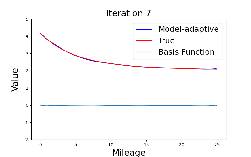
Our method takes 15 iterations to solve the equation. Figure 1 visualizes our approximation solution for the first 9 iterations and the basis functions. Each panel shows the impact on the approximate solution of adding one additional sieve basis function to the previous value.

Figure 1: Convergence Behavior of Model-Adaptive Approach

Figure 2: Norms of residuals and approximation error for Bus Engine Replacement

Figure 2 plots the $L_{2}$-norm of the residuals and the sup-norm of the approximation error. The approximation solution is close to the true solution after iteration 6, which implies that our algorithm constructs a good sieve space using 6 iterations. After that, the approximation converges to the true solution rapidly. This finding aligns with Figure 2 as the approximation error dramatically decreases at iteration 6-7. Other norms also decay dramatically after 6 iterations. Moreover, the $L_{2}$-norm of the approximation errors decreases monotonically, consistent with Theorem 3.

5.2 Consumer Demand for Storable Goods

In this section, we analyze a model of consumer demand for storable goods similar to Hendel and Nevo (2006). We aim to show that our method opens the door to the use of Bayesian MCMC estimation methods for such models.

At each period, given prices $\bm{p}$ and inventories $I$, a household of size $n$ decides which brand $k$ to purchase, how much to purchase $j$ and how much to consume $C$. Let $\omega_{j}\left(\bm{p}\right)$ be the indirect utility from brand choice and $x:=\{\bm{\omega},I\}$. Given the assumptions in Hendel and Nevo (2006), brand choice is purely a static problem and the consumer’s value function $V(x)$ for the dynamic problem is the solution to:

$$V(x)=\log\sum_{j}\exp(U(C(x,j),I,j;\theta)+\omega_{j}\left(\bm{p}\right)+\beta\mathbb{E}[V(x^{\prime})|x,C(x,j),j])$$

where $C(x,j):=\operatornamewithlimits{argmax}_{c_{min}\leq c\leq c_{max}}\Bigl[U(c,I,j;\theta)+\omega_{j}\left(\bm{p}\right)+\beta\mathbb{E}[V(x^{\prime})|x,c,j]\Bigr]$.

We compare several solution methods combining two outer iteration frameworks (PI and NK) with different inner solvers (MA, SA, and an exact linear equation solver), along with VFI and one-step VFI as benchmarks. The pseudocode for PI+MA and its VFI and one-step VFI variants is given in Appendix B.2. For a given consumption function, we update the value function using either PI or NK outer iterations with the chosen inner solver, then update the consumption function and iterate until convergence. The one-step updating was used in Osborne (2018) to implement the Bayesian estimator proposed by Imai et al. (2009)—henceforth, IJC. At each MCMC step, rather than iterate to convergence, the algorithm updates both the value function and the consumption function only by one-step.

Table 1 compares the computational time and number of iterations required by each algorithm across simulations for different household sizes. NK+MA is the fastest method, requiring approximately 0.5 minutes across all household sizes, followed by PI+MA at around 0.7 minutes. NK+SA requires about 1.0 minutes and PI+SA about 2.4 minutes. Exact solution takes about 4.6 minutes. VFI converges in about 1.5 minutes. These results demonstrate that combining MA with NK outer iterations substantially improves computational efficiency. One-step VFI requires about 64 minutes, more than 100 times slower than NK+MA.

Table 1: Performance of Solution Algorithms

	Time in mins					Number of Iterations
Household Size	1	2	3	4	5	1	2	3	4	5
PI + MA	0.7	0.8	0.8	0.7	0.5	6	7	7	6	5
PI + SA	2.2	2.6	2.7	2.4	1.9	6	7	7	6	5
PI + Exact	4.4	4.6	5.2	5.0	3.6	6	7	7	6	5
NK + MA	0.5	0.6	0.6	0.5	0.4	6	7	7	6	5
NK + SA	0.9	1.2	1.1	0.9	0.8	6	7	7	6	5
VFI	1.5	1.8	1.6	1.5	1.3	6	7	7	6	5
One-step VFI	63.7	64.2	64.1	65.6	63.7	1621	1639	1649	1649	1645

Note: The computational time is the real time in minutes. The code runs on an Intel Xeon Gold 6240 CPU (2.60GHz) with 192GB RAM.

Our method opens the door to the use of Bayesian MCMC estimators. To simulate 10,000 MCMC steps, Table 8 shows that PI+MA requires between 1.6 and 3.3 days depending on household size.

An alternative estimator to the Bayesian MCMC estimator is the IJC approach. However, the performance of the one-step VFI suggests that the IJC approach may not be the most suitable estimator for this problem. In Table 1, the one-step VFI approach requires more than 1600 iterations to converge even when the true parameters are known. Consequently, due to the extremely large number of iterations required, we expect the total computational time using the IJC approach would be substantially higher than our proposed approach.

5.3 Single Firm Entry and Exit

This section examines a single-firm entry and exit problem described in Aguirregabiria and Magesan (2023). We compare the performance of the model-adaptive approach (MA) against successive approximation (SA) and temporal difference (TD) as inner solvers for the linear system (2.3). These inner solvers are embedded within policy iteration (PI) and Newton–Kantorovich (NK) outer iterations. We also include value function iteration (VFI) as a benchmark and examine how computational time scales with the state space size.

5.3.1 Design of the Simulation

At each period $t\leq+\infty$, a firm decides whether to exit ($a_{t}=0$) or enter ($a_{t}=1$) the market. For an active firm, the profit is $\pi(1,x_{t})+\varepsilon_{t}(1)$. $\pi(1,x_{t})$ equals the variable profit $VP_{t}$ minus fixed cost $FC_{t}$, and minus entry cost $EC_{t}$. For an inactive firm, $\pi(0,x_{t})$ is normalized to be 0, and the profit is $\varepsilon_{t}(0)$. The variable profit is $VP_{t}=(\theta_{0}^{VP}+\theta_{1}^{VP}z_{1t}+\theta_{2}^{VP}z_{2t})\exp(w_{t})$ where $w_{t}$ is the productivity shock, $z_{1t}$ and $z_{2t}$ are exogenous state variables that affect price-cost margin. The fixed cost is $FC_{t}=\theta_{0}^{FC}+\theta_{1}^{FC}z_{3t}$, and the entry cost is $EC_{t}=(1-a_{t-1})(\theta_{0}^{EC}+\theta_{1}^{EC}z_{4t})$ where $(1-a_{t-1})$ indicates that the entry cost is paid if the firm is inactive at the previous period ($a_{t-1}=0$). Continuous state variables follow AR(1) process: $z_{jt}=0.6z_{jt-1}+\epsilon_{jt}$, $w_{t}=0.2+0.6w_{t-1}+\epsilon_{t}$, where $\epsilon_{jt}$, $\epsilon_{t}$ follows i.i.d standard normal. The true parameters $\theta^{*}$ are chosen to be $\theta_{0}^{VP}=0.5,\theta_{1}^{VP}=1,\theta_{2}^{VP}=-1,\theta_{0}^{FC}=1.5,\theta_{1}^{FC}=1,\theta_{0}^{EC}=1,\theta_{1}^{EC}=1$. We use $M$-point Tauchen’s method (Tauchen (1986)) to discretize each of 5 continuous state variables and obtain the transition matrix where $M=\{6,7,8,9,10\}$. Moreover, we set the discount factor $\beta=\{0.95,0.975,0.980,0.985,0.990,0.995,0.999\}$.

5.3.2 Kronecker Product Structure

The transition matrix $F$ admits a Kronecker product factorization $F=F_{a}\otimes F_{1}\otimes F_{2}\otimes\cdots\otimes F_{d}$, where $F_{a}$ corresponds to the discrete action state and each $F_{j}$ is the $M\times M$ Tauchen transition matrix for the $j$-th continuous variable. This structure allows computing the matrix-vector product $Fv$ without ever forming or storing $F$ explicitly. The cost of one matrix-vector product is $O(dM|\mathcal{X}_{M}|)$, compared with $O(|\mathcal{X}_{M}|^{2})$ for a dense matrix-vector product. Since each MA iteration requires two such products (one with $(\mathcal{I}-\beta F)$ and one with its adjoint), the total cost of $k$ MA iterations is $O(k\,d\,M\,|\mathcal{X}_{M}|)$. The memory requirement is $O(dM^{2}+|\mathcal{X}_{M}|)$—storing $d$ matrices of size $M\times M$ plus the iterate—rather than $O(|\mathcal{X}_{M}|^{2})$ for the dense matrix.

5.3.3 Method Comparison

We compare the computational performance of the above methods for solving the dynamic programming problem with $M=6$ grid points per dimension ($|\mathcal{X}_{M}|=15{,}552$) and $\beta=0.95$. All methods exploit the Kronecker product structure of the transition matrix for efficient matrix-vector multiplication.

Table 2 presents the results. Panel A reports the solve time for the linear system (2.3) given the true CCP, which is obtained by solving the DP problem to convergence using VFI. MA converges in 120 iterations (0.16 seconds), outperforming SA which requires 389 iterations (0.21 seconds). TD produces a large residual of $5.31\times 10^{2}$, indicating that the polynomial sieve space is inadequate for approximating the value function in this model.

Panel B compares full-solution methods that solve the DP problem directly. VFI converges in 479 iterations (1.06 seconds). Among PI-based methods, PI+MA (0.72 seconds) outperforms PI+SA (0.91 seconds). NK+MA achieves the fastest total time (0.44 seconds). The speed advantage of NK over PI reflects two factors: NK converges in 4 outer iterations versus 5 for PI, and its quadratic outer convergence yields fewer total inner iterations (307 versus 514).

Table 2: Numerical Experiment: Method Comparison

Panel A: Given true CCP					Panel B: Full-solution methods
Method	Time (s)	Iters	Residual		Method	Time (s)	Iters
MA	0.16	120	—		VFI	1.06	479
SA	0.21	389	—		PI + MA	0.72	514
TD	0.12	—	$5.31\times 10^{2}$		PI + SA	0.91	1,922
					NK + MA	0.44	307

Note: $|\mathcal{X}_{M}|=2\times 6^{5}=15{,}552$, $\beta=0.95$. Panel A reports solve time for the linear system given the true CCP. Panel B reports total time to solve the DP problem. For PI and NK methods, Iters is the total number of inner solver iterations across all outer iterations. PI converges after 5 outer iterations and NK after 4. The code runs on an Intel Xeon Gold 6240 CPU (2.60GHz) with 192GB RAM.

In Figures 4, 4, 6 and 6, we visualize the convergence of MA for $M=6$ given the true CCP. We plot the sup-norm of residuals, $\|r_{k}\|_{\infty}$, $L_{2}$-norm of the residuals, $\|r_{k}\|_{2}$, the sup-norm of the approximation error, $\|V_{k}-V^{*}\|_{\infty}$, and $L_{2}$ norm of the approximation error, $\|V_{k}-V^{*}\|_{2}$. All figures are plotted as functions of the iteration count $k$ for different $\beta$. Figures 4, 4 and 6 exhibit a similar pattern: they increase initially, reach a peak, and then decrease rapidly. Figure 6 shows the $L_{2}$-norm of approximation error decreases monotonically consistent with Theorem 3. Notably, while $\beta=0.999$ initially results in larger residuals and approximation errors compared to smaller discount factors, it still achieves convergence within a comparable number of iterations. This demonstrates the ability of MA to handle large discount factors, which is challenging for SA.

Figure 3: Sup-norm of Residuals

Figure 4: $L_{2}$-Norm of Residuals

Figure 5: Sup-norm of Approx. Error

Figure 6: $L_{2}$-Norm of Approx. Error

5.3.4 Scaling with State Space Size

We examine how the computational cost of PI+MA scales with the state space size. Table 3 presents the average number of MA iterations and average computational time per policy iteration step for $M=6,7,8,9,10$. PI converges after 5 iterations for all $M$ and $\beta$.

These results provide empirical support for Theorem 5. As $M$ increases, the average number of iterations remains relatively stable for all $\beta$, consistent with the mesh independence property. For instance, at $\beta=0.95$, the average number of iterations is 103 for $M=6$ and 96 for $M=10$. The computational time scales approximately linearly in $|\mathcal{X}_{M}|$, consistent with the $O(d\,M\,|\mathcal{X}_{M}|)$ cost of Kronecker matrix-vector multiplication described in Section 5.3.2. Additionally, there is a slight increase in the average number of iterations (from around 96 to 120) as $\beta$ increases from 0.95 to 0.999 at $M=10$. As it only takes up to 1.5 seconds per policy iteration step to solve the linear equation with $|\mathcal{X}_{M}|=200{,}000$, MA improves the computational efficiency of policy iteration where the main computational cost is solving the linear system of equations.

Table 3: Numerical Experiment: Performance for Different $\beta$ and $M$

	Avg Number of Iterations						Avg Time in secs
$\beta$	$M=6$	$M=7$	$M=8$	$M=9$	$M=10$		$M=6$	$M=7$	$M=8$	$M=9$	$M=10$
0.950	103	101	100	98	96		0.14	0.21	0.39	0.66	1.18
0.975	110	109	107	105	103		0.14	0.23	0.41	0.68	1.25
0.980	112	111	109	107	105		0.17	0.23	0.43	0.71	1.27
0.985	114	113	111	109	107		0.15	0.23	0.43	0.73	1.29
0.990	116	115	114	112	110		0.15	0.24	0.43	0.75	1.32
0.995	120	118	117	115	113		0.15	0.25	0.45	0.77	1.37
0.999	125	124	123	121	120		0.16	0.25	0.46	0.81	1.46
$|\mathcal{X}_{M}|$	15,552	33,614	65,536	118,098	200,000		15,552	33,614	65,536	118,098	200,000

Note: $|\mathcal{X}_{M}|:=2\times M^{5}$ is the cardinality of the state space. All DP problems converge after 5 policy iterations. Avg number of iterations and avg time refer to the average across 5 PI steps. The code runs on an Intel Xeon Gold 6240 CPU (2.60GHz) with 192GB RAM.

6 Empirical Application

This section applies our method to a dynamic consumer demand model for laundry detergent using Kantar’s Worldpanel Take Home data. We first describe the data, model, and estimation procedure. Then, we discuss the implication of the results.

6.1 Data

The analysis of the Great Britain laundry detergent industry is based on the data from 1st January 2017 until 31st December 2019. It captures detailed information on a representative sample of British households’ purchases of fast-moving products, including food, drink, and laundry detergents. The data has been used in previous studies such as Dubois et al. (2014, 2020). Households use barcode scanners to record all their grocery purchases. For each purchase, the data includes key information such as price, quantity, product characteristics, and purchase date.

We consider the market for laundry detergent. A laundry detergent product is defined by its quantity, brand, and chemical properties (bio/non-bio). Laundry detergents are available in various formats such as liquid, powder, and gel, each with different dosage metrics. To standardize quantity across formats, we define the quantity purchased by the number of washes. Table 4 presents the top 10 brands and bio/non-bio combinations, which account for 76.82% of the total observed purchases. We restrict our analysis to these top 10 brand and bio/non-bio combinations, and assume they are available to all consumers.

Table 4: Market Share of Top 10 Brands and Bio/Non-Bio

Brand + Bio	1	2	3	4	5	6	7	8	9	10
Number of observations	41,427	40,954	33,164	32,604	29,213	26,087	21,768	17,371	17,334	15,945
Cumulative share (%)	11.54	22.94	32.18	41.26	49.39	56.65	62.72	67.55	72.38	76.82

Note: Number of observations for top 10 brand and bio/non-bio combination between 1st January 2017 and 31st December 2019, using Kantar’s Worldpanel Take Home data.

In Figure 7 we show the histogram of quantities purchased, which suggests three natural clusters corresponding to small, medium, and large sizes. Therefore, we use $3$-means clustering to aggregate the quantities for each brand and bio/non-bio combination into small (23), medium (40), and large (64) sizes. Table 5 summarizes the number of observations for each cluster. We then calculate the weekly average transaction price for each product cluster, and use it as the price index in our model.

Figure 7: Histogram of Quantities Purchased

Table 5: $3$-means Clustering of Quantities Purchased

	Brand + Bio
Washes	1	2	3	4	5	6	7	8	9	10
23	20,928	24,946	20,066	28,564	12,134	6,370	5,832	15,554	10,896	6,280
40	13,265	11,938	9,370	3,789	10,075	11,802	9,634	1,720	5,052	7,783
64	7,234	4,070	3,728	0	7,004	7,915	6,302	0	1,386	1,882

Note: ”Washes” refers to number of washes. Number of observations for $3$-means clustering of quantities purchased for each brand and bio/non-bio combination between 1st January 2017 and 31st December 2019, using Kantar’s Worldpanel Take Home data.

In Table 6 we describe purchase statistics by household size. We restrict our analysis to households who purchase laundry detergent at least 3 times and at most 15 times each year for household sizes 1-4, and 3 to 20 times each year for household size 5. The average size of laundry detergent purchased increases with household size, ranging from 32.2 washes per purchase for single-person households to 38.1 washes for households with four or five. The average price per wash, conditional on purchase, shows a slight decreasing trend as household size increases, from £0.152 for single-person households to £0.142 for the largest households. The average number of weeks between purchases decreases as household size increases, with single-person households making purchases every 9.7 weeks on average, while households with five members purchase every 7.4 weeks. The average quantity of laundry detergent purchased per year increases with household size, ranging from 165 washes per year for single-person households to 256 washes for the largest households. Table 6 indicates heterogeneity in purchasing behavior across different household sizes. Therefore, we separately estimate the model for each household size.

Table 6: Laundry Detergent Purchase Statistics by Household Size

Household Size	1	2	3	4	5
Avg. Size conditional on purchase	32.2	35.2	36.6	38.1	38.1
Avg. Price per wash conditional on purchase	0.152	0.146	0.145	0.143	0.142
Avg. Weeks between purchases	9.7	8.6	7.8	7.6	7.4
Avg. Quantity purchased per Year	165	203	232	247	256
Number of households	235	772	351	373	117

Note: The purchase statistics are based on Kantar’s Worldpanel Take Home data between 1st January 2017 and 31st December 2019.

6.2 Model

In the model, laundry detergent is storable, and households derive utility from both consumption and purchase. As in Hendel and Nevo (2006), we assume that laundry detergents are perfect substitutes in consumption, which implies that the unobserved state variable, inventory, is one-dimensional. At week $t\leq+\infty$, consumer $i$ chooses discrete consumption $c_{t}$ and purchase decision $a_{jklt}$, where $j\in\{0,23,40,64\}$ is the quantity measured by the number of washes, $k$ refers to the brand, and $l$ is bio/non-bio. Let $\bm{a}_{t}$ be a vector of purchase decisions with $\sum_{j,k,l}a_{jklt}=1$, where $a_{jklt}=1$ indicates the purchase of quantity $j$ of brand $k$ and bio/non-bio $l$, and $a_{jklt}=0$ otherwise. The period utility is given by:

$$u(\bm{a}_{t},c_{t},I_{t},\bm{p}_{t},\varepsilon_{t};\theta)=\theta_{1}c_{t}+\theta_{2}c_{t}^{2}+\theta_{3}{I}_{t+1}^{2}+\theta_{4}\mathbbm{1}(\sum_{j>0,k,l}a_{jklt}>0)+\sum_{j,k,l}a_{jklt}(\theta_{5}p_{jklt}+j\xi_{k}+j\delta_{l}+\varepsilon_{jklt})$$

where $I_{t}$ is the inventory at the beginning of $t$ and $\bm{p}_{t}$ is a vector of prices. $\varepsilon_{jklt}$ is the choice-specific utility shock following an i.i.d. Type I Extreme Value distribution. $(\theta_{1},\theta_{2})$ capture the marginal utility of consumption. $\theta_{3}$ captures the carrying cost that depends on the inventory at next period: $I_{t+1}:=I_{t}+j_{t}-c_{t}$. The fixed cost of making a purchase is $\theta_{4}$. We impose an upper bound on the inventory $I_{t}\in\{0,1,\cdots,I_{max}\}$ where $I_{max}=80$. The consumption is bounded from below and above by $c_{min,t}:=\max\{0,I_{t}+j_{t}-I_{max}\}$ and $c_{max,t}:=I_{t}+j_{t}$, respectively. $\theta_{5}$ captures the price sensitivity. $\xi_{k}$ and $\delta_{l}$ are brand and bio/non-bio fixed effects per wash.

A household maximizes expected life-time utility:

$$\max_{\{\bm{a}_{t},c_{t}\}_{t=0}^{\infty}} \mathbb{E}\left[\sum_{t=0}^{+\infty}\beta^{t}u(\bm{a}_{t},I_{t},\bm{p}_{t},\varepsilon_{t};\theta)|I_{0},\bm{p}_{0}\right]$$

s.t. $$c_{t}\in[c_{min,t},c_{max,t}]$$

$$I_{t+1}:=I_{t}+j_{t}-c_{t}$$

where $\beta=0.99$. The state space is defined by $s_{t}:=(I_{t},\bm{p}_{t})$.

6.3 Estimation Overview

This section presents the estimation procedure. We mainly follow the three-step procedure in Hendel and Nevo (2006). We assume $\bm{p}_{t}$ follows an exogenous first-order Markov process. Therefore, inventory $I_{t}$ is the only endogenous state variable. This allows us to decompose the decisions into dynamic decisions $(c_{t},j_{t})$ and static decisions $(k_{t},l_{t})$, as the evolution of $I_{t}$ is determined only by $(c_{t},j_{t})$. Moreover, as shown in Hendel and Nevo (2006), the choice probability of purchasing brand $k$ and bio/non-bio $l$ conditional on purchasing quantity $j$ has the conditional logit form:

$$Pr(k,l|\bm{p},j)=\frac{\exp(\theta_{5}p_{jkl}+j\xi_{k}+j\delta_{l})}{\sum_{k,l}\exp(\theta_{5}p_{jkl}+j\xi_{k}+j\delta_{l})}$$

allowing for simple estimation of $(\theta_{5},\xi_{k},\delta_{l})$.

Then, the inclusive value of purchasing quantity $j$ is defined by:

$$\omega_{j,t}=\log\left[\sum_{k,l}\exp(\theta_{5}p_{jklt}+j\xi_{k}+j\delta_{l})\right]$$

where $\omega_{j,t}$ is the indirect utility of purchasing quantity $j$ at period $t$. We impose the inclusive value sufficiency (IVS) assumption as in Hendel and Nevo (2006):

Assumption 3 (Inclusive Value Sufficiency).

$F(\bm{\omega}_{t}|\bm{p}_{t-1})$ can be summarized by $F(\bm{\omega}_{t}|\bm{\omega}_{t-1})$ where $F$ is the conditional distribution function.

Given Assumption 3, the lagged inclusive value $\bm{\omega}_{t-1}$ is a sufficient statistic to forecast $\bm{\omega}_{t}$. As a result, the state space can be reduced from $s_{t}:=(I_{t},\bm{p}_{t})$ to $x_{t}:=\{I_{t},\bm{\omega}_{t}\}$. We forecast $\bm{\omega}_{t}$ using a VAR(1) and then discretize it into $5^{3}$ bins. The simplified dynamic programming problem based on the IVS assumption is:

$$V(x,\varepsilon)=\max_{j,c_{min}\leq c\leq c_{max}}\Bigl[U(c,I,j;\theta)+\omega_{j}+\varepsilon(j)+\beta\mathbb{E}[V(x^{\prime})|x,c,j]\Bigr]$$

where $U(c,I,j;\theta)=\theta_{1}c+\theta_{2}c^{2}+\theta_{3}I^{\prime 2}+\theta_{4}\mathbbm{1}(j>0)$, $I^{\prime}:=I+j-c$ is next-period inventory, $\varepsilon$ is a 4-dimensional vector of i.i.d Type I Extreme Value distribution, and $V(x)=\mathbb{E}_{\varepsilon}V(x,\varepsilon)$.

We decompose the joint optimization problem into sequential optimization problems: first choose purchase quantity $j$, then choose consumption. For the second problem, given state $x$, purchase quantity $j$, and $V(x)$, define the consumption function as:

$$C(x,j):=\operatornamewithlimits{argmax}_{c_{min}\leq c\leq c_{max}}\Bigl[U(c,I,j;\theta)+\omega_{j}+\beta\mathbb{E}[V(x^{\prime})|x,c,j]\Bigr]$$ (6.1)

For the first problem, the choice probability of purchasing quantity $j$ is:

$$p(j|x)=\frac{\exp(v(x,j))}{\sum_{j^{\prime}}\exp(v(x,j^{\prime}))}$$

where $v(x,j):=U(C(x,j),I,j;\theta)+\omega_{j}+\beta\mathbb{E}[V(x^{\prime})|x,C(x,j),j]$. Combining these two steps, we have:

$$V(x)=\log\sum_{j}\exp(U(C(x,j),I,j;\theta)+\omega_{j}+\beta\mathbb{E}[V(x^{\prime})|x,C(x,j),j])$$ (6.2)

For a given consumption function, we solve (6.2) by policy iteration with our model-adaptive approach. Then, we update the consumption function using (6.1), and iterate until convergence (see 4).

As the argmax operator in 4 for discrete outcomes is not differentiable, we estimate the dynamic parameters by the Bayesian MCMC estimator. The estimation details are described in Appendix B.3.

6.4 Results and Implications

We separately estimate the model for different household sizes. Table 7 presents the results of the conditional logit model. The coefficient $\theta_{5}$ measures the price sensitivity, which is negative and statistically significant at 5% level across all household sizes. Single-person households exhibit the highest price sensitivity at -0.501, followed by households with three members at -0.416, households with two members at -0.345, and households with four members at -0.307. Five-person households have the lowest price sensitivity at -0.223. The estimates also suggest the heterogeneity in price sensitivity across different household sizes.

Table 7: Conditional Logit: Brand and Bio Choice Conditional on Quantity

Household Size	1	2	3	4	5
$\theta_{5}$	-0.501	-0.345	-0.416	-0.307	-0.223
	(0.029)	(0.014)	(0.020)	(0.018)	(0.030)
Brand FE      * Quantity	Yes	Yes	Yes	Yes	Yes
Bio FE      * Quantity	Yes	Yes	Yes	Yes	Yes

Note: Standard errors are in parentheses. Estimates of a conditional logit model. We use the transaction price for the observed purchase and the price index for other choices.

In Table 8 we report the estimates of dynamic parameters and computational times. All estimates have the expected signs and are statistically significant at the 5% level. The utility from consumption, determined jointly by the linear term ($\theta_{1}$) and quadratic term ($\theta_{2}$), shows varying patterns across household types. The linear coefficient $\theta_{1}$ ranges from its lowest value of 1.878 for four-person households to its peak of 3.583 for three-person households. Five-person households have the lowest magnitude for the quadratic term $\theta_{2}$ (-8.423). Single-person households have the lowest fixed cost of making a purchase ($\theta_{4}=-4.195$), while five-person households have a relatively high fixed cost ($\theta_{4}=-5.349$). The average time ranges from 0.23 to 0.48 minutes per Metropolis–Hastings step. The total time of the MCMC estimator ranges from 1.6 to 3.3 days, which confirms the computational efficiency of PI+MA in practice.

Table 8: Estimation Results and Computational Time

Household Size	1	2	3	4	5
$\theta_{1}$	2.069	2.663	3.583	1.878	1.909
	(0.386)	(0.186)	(0.276)	(0.284)	(0.577)
$\theta_{2}$	-13.910	-14.840	-14.071	-11.115	-8.423
	(0.879)	(0.466)	(0.579)	(0.481)	(0.757)
$\theta_{3}$	-3.230	-2.242	-3.215	-3.474	-4.246
	(0.238)	(0.079)	(0.154)	(0.365)	(1.035)
$\theta_{4}$	-4.195	-4.868	-4.927	-5.281	-5.349
	(0.086)	(0.041)	(0.064)	(0.070)	(0.149)
Avg Time (mins)	0.48	0.23	0.27	0.29	0.39
Total Time (days)	3.3	1.6	1.9	2.0	2.7

Note: The first 8,000 of 10,000 MCMC draws are discarded as burn-in. The means are taken over last 2,000 MCMC draws. The standard errors (in parentheses) are the standard deviation of the MCMC draws. The computational time is the average time per Metropolis–Hastings step. The code runs on an Intel Xeon Gold 6240 CPU (2.60GHz) with 192GB RAM.

To investigate the model fit, we compare the simulated and observed purchase behavior. For each household size, we simulate consumption and purchase behavior for the same number of households as observed in the data over 156 weeks (3 years). The simulated market shares in Table 9 reasonably match the observed data. Figure 8 plots the hazard rates and their confidence intervals. We also estimate the static model without the carrying cost. All household sizes exhibit a similar pattern, with the hazard rates initially increasing until stabilizing at the highest level. For single-person and two-person households, the hazard rates increase until around 8 weeks, while the hazard rates increase until around 5 weeks for larger households. The hazard rates all peak around 15%. The dynamic model outperforms the static model in capturing the hazard rates as the static model, by construction, cannot capture the increasing hazard rate observed in the data.

Table 9: Model Fitting for Different Household Sizes: Market Share

Household Size		Small	Medium	Large
1	Observed	5.76 (0.14)	2.96 (0.11)	1.09 (0.06)
	Simulated	5.48 (0.14)	3.23 (0.11)	0.93 (0.06)
2	Observed	5.38 (0.08)	3.90 (0.07)	1.78 (0.05)
	Simulated	5.17 (0.08)	4.13 (0.07)	1.59 (0.04)
3	Observed	5.27 (0.11)	4.66 (0.11)	2.14 (0.07)
	Simulated	5.16 (0.11)	4.64 (0.11)	2.07 (0.07)
4	Observed	4.94 (0.11)	4.66 (0.10)	2.78 (0.08)
	Simulated	4.74 (0.10)	4.85 (0.11)	2.68 (0.08)
5	Observed	4.90 (0.19)	4.90 (0.19)	2.71 (0.14)
	Simulated	4.86 (0.19)	4.70 (0.19)	2.50 (0.14)

Note: Values represent percentages. We simulate the same number of households as observed in the data over 156 weeks and discard the first 30% periods of both the simulated and observed data. The standard errors of the simulated and observed data are in parentheses.

Note: For each household size, we simulate the same number of households as observed in the data over 156 weeks and discard the first 30% periods of both the simulated and observed data. In each figure, the light blue and orange lines represent the 95% confidence intervals of the hazard rates for the observed and simulated data, respectively.

Figure 8: Hazard Rates of Purchase Across Different Household Sizes

Long-run elasticities measure the effects of permanent price changes on market shares. Table 10 simulates the long-run elasticities for different household sizes. Own-price elasticities are larger in absolute value for larger pack sizes. They are all greater than 1 in absolute value, except the small pack for household size 5 (-0.742), indicating that the demand is generally elastic. For single-person households, the own-price elasticity for large packs is -4.067, meaning that if the prices of all large packs increase by 1%, the market shares of large packs will decrease by 4.067%. As household size increases, there is a trend towards lower price elasticities, suggesting that larger households are less sensitive to price changes. This trend can partially be explained by the price coefficients ($\theta_{5}$) as larger households are less price sensitive, except for household size 3, as shown in Table 7.

The demand for each size is elastic in general, indicating consumers are likely to substitute out of the pack size that has increased in price and to other pack sizes or not purchase at all. For single-person households, the cross-price elasticity between medium and large packs is 0.601, higher than the cross-price elasticity between medium and small packs (0.256). This pattern continues across household sizes - for 2-person households, the medium-large cross-price elasticity is 0.378, for 3-person households it increases to 0.628, showing stronger substitution effects for larger sizes. The cross-elasticities between medium and small packs remain relatively stable across household sizes (ranging from 0.256 to 0.268 for households of 1-3 persons), while the substitution effects involving large packs tend to be stronger. These findings suggest that consumers are more likely to substitute between larger pack sizes when prices change, particularly in households with 2-3 members, though this effect diminishes somewhat for the largest households. Overall, the magnitudes of our long-run elasticities are consistent with prior estimates in the literature: Hendel and Nevo (2006) report long-run own-price elasticities between $-2.5$ and $-4.3$ for 128 oz. liquid detergent, which aligns well with our estimates for larger pack sizes.

Table 10: Long Run Elasticities for Different Household Sizes

Household Size		Small	Medium	Large
	Small	-1.619 (0.060)	-0.223 (0.058)	-0.437 (0.096)
1	Medium	-0.256 (0.078)	-2.425 (0.087)	-0.601 (0.159)
	Large	-0.102 (0.059)	-0.253 (0.079)	-4.067 (0.190)
	Small	-1.128 (0.047)	-0.215 (0.034)	-0.162 (0.048)
2	Medium	-0.258 (0.055)	-1.593 (0.049)	-0.378 (0.057)
	Large	-0.174 (0.051)	-0.230 (0.055)	-2.602 (0.112)
	Small	-1.463 (0.055)	-0.277 (0.038)	-0.231 (0.054)
3	Medium	-0.268 (0.068)	-1.976 (0.052)	-0.628 (0.065)
	Large	-0.187 (0.064)	-0.372 (0.069)	-2.992 (0.126)
	Small	-1.012 (0.055)	-0.078 (0.051)	-0.217 (0.051)
4	Medium	-0.185 (0.063)	-1.419 (0.046)	-0.330 (0.045)
	Large	-0.173 (0.067)	-0.274 (0.059)	-2.220 (0.070)
	Small	-0.742 (0.040)	-0.043 (0.030)	-0.103 (0.039)
5	Medium	-0.102 (0.068)	-1.034 (0.056)	-0.178 (0.037)
	Large	-0.127 (0.061)	-0.160 (0.064)	-1.657 (0.073)

Note: We increase the price of each pack size by 1% to simulate the long-run elasticities. For each of the 2000 MCMC draws, we solve the dynamic programming problem, simulate 1000 households over 2000 weeks and discard the first 30% periods. The means are taken over the 2000 MCMC draws. The standard errors (in parentheses) are the standard deviations of simulated elasticities across 2000 MCMC draws.

7 Conclusion

In this paper, we propose a model-adaptive approach to solve the linear system of fixed point equations of the policy valuation operator. Our method adaptively constructs the sieve space and chooses its dimension. It converges superlinearly, while conventional methods do not. We demonstrate through simulations that our model-adaptive sieves dramatically improve the computational efficiency of policy iteration and Newton–Kantorovich iterations, and open the door to the use of Bayesian MCMC estimators for DDC models.

We apply our method to analyze consumer demand for laundry detergent using Kantar’s Worldpanel Take Home data. The empirical application confirms that our approach improves computational efficiency of policy iteration in practice, which opens the door to the estimation of DDC models by Bayesian MCMC estimators. To investigate the model fit, we simulate market shares and hazard rates for different household sizes. The model achieves a reasonable model fit. We also simulate the long-run elasticities. The results show the heterogeneous substitution patterns across different household sizes.

Appendix A Proofs

Let $\mathcal{K}:=\mathcal{T}+\mathcal{T}^{*}-\mathcal{T}\mathcal{T}^{*}$. The constants in this section can vary from line to line.

Proof of Theorem 1.

1. By Lemma 2, it suffices to show that $(\mathcal{I}-\mathcal{T}^{*})$ is invertible on $L^{2}(\mathbb{X})$. By Assumption 1(v), we have $(\mathcal{I}-\mathcal{T})$ is a bounded operator on $L^{2}(\mathbb{X})$, since $\|\mathcal{I}-\mathcal{T}\|_{op}\leq 1+\|\mathcal{T}\|_{op}\leq 1+\|\mathcal{T}\|_{HS}<+\infty$ where we used $\mathcal{T}$ is a Hilbert–Schmidt operator as shown in Lemma 4. Thus, it is continuous by Kress (2014) Theorem 2.3. By Lemma 1, $L^{2}(\mathbb{X})$ is a separable Hilbert space. Moreover, $(\mathcal{I}-\mathcal{T})$ is bijective as it is invertible on $L^{2}(\mathbb{X})$ as shown in Lemma 2. Thus, by the bounded inverse theorem (e.g., Narici and Beckenstein (2010)), $(\mathcal{I}-\mathcal{T})^{-1}$ is also bounded. By Reed and Simon (1980) Theorem VI.3 (d), the adjoint operator $(\mathcal{I}-\mathcal{T}^{*})$ is invertible and has a bounded inverse on $L^{2}(\mathbb{X})$.

2. Let $V^{*}$ be the unique solution to $(\mathcal{I}-\mathcal{T})V=u$ on $L^{2}(\mathbb{X},\mu)$. Note that $(\mathcal{I}-\mathcal{T}^{*})y^{*}$ is the solution to $(\mathcal{I}-\mathcal{T})V=u$ on $L^{2}(\mathbb{X})$. Since the norm $\|\cdot\|_{\mu}$ and $\|\cdot\|$ are equivalent, $(\mathcal{I}-\mathcal{T}^{*})y^{*}\in L^{2}(\mathbb{X},\mu)$. Therefore, $(\mathcal{I}-\mathcal{T}^{*})y^{*}$ is also the solution on $L^{2}(\mathbb{X},\mu)$. As $(\mathcal{I}-\mathcal{T})V=u$ has a unique solution on $L^{2}(\mathbb{X},\mu)$, we have $(\mathcal{I}-\mathcal{T}^{*})y^{*}=V^{*}$, $\mu$-a.s.

∎

Proof of Theorem 2.

1. Lemma 6(i) proves the orthogonality.

2. Let $\|h\|^{2}_{(\mathcal{I}-\mathcal{K})}:=\langle(\mathcal{I}-\mathcal{K})h,h\rangle$. By Han and Atkinson (2009) page 251, we have:

   $$y_{k}=\operatornamewithlimits{argmin}_{y\in\text{span}\{r_{0},r_{1},\cdots,r_{k-1}\}}\|y-y^{*}\|_{(\mathcal{I}-\mathcal{K})}$$

   Note that:

   $$\|y_{k}-y^{*}\|^{2}_{(\mathcal{I}-\mathcal{K})} =\langle(\mathcal{I}-\mathcal{T})(\mathcal{I}-\mathcal{T}^{*})(y_{k}-y^{*}),(y_{k}-y^{*})\rangle$$

   $$=\langle(\mathcal{I}-\mathcal{T}^{*})(y_{k}-y^{*}),(\mathcal{I}-\mathcal{T}^{*})(y_{k}-y^{*})\rangle$$

   $$=\|(\mathcal{I}-\mathcal{T}^{*})(y_{k}-y^{*})\|^{2}=\|(\mathcal{I}-\mathcal{T}^{*})y_{k}-V^{*}\|^{2}$$

   Therefore, we have $y_{k}=\operatornamewithlimits{argmin}_{y\in\text{span}\{r_{0},r_{1},\cdots,r_{k-1}\}}\|(\mathcal{I}-\mathcal{T}^{*})y_{k}-V^{*}\|$.

∎

Proof of Theorem 3.

As $\mathcal{K}$ is a compact self-adjoint operator shown in Lemma 5, its eigenvalues are real and countable. Without loss of generality, we assume the eigenvalues are ordered as follows: $|\lambda_{1}|\geq|\lambda_{2}|\geq\cdots\geq 0$ where $\lim_{j\to\infty}|\lambda_{j}|=0$. The eigenvalues of $(\mathcal{I}-\mathcal{K})$ are $\{1-\lambda_{j}\}_{j\geq 1}$. By Kress (2014) Theorem 15.11 and Definition 3.8, we have $\Delta:=\|\mathcal{I}-\mathcal{K}\|_{op}=\sup_{j}(1-\lambda_{j})$. Since $(\mathcal{I}-\mathcal{K})$ is positive definite, we have $\Delta>0$. By Kress (2014) Theorem 3.9, zero is the only possible accumulation point of the eigenvalues $\{\lambda_{j}\}_{j\geq 1}$. Thus, $\delta:=\inf_{j}(1-\lambda_{j})>0$. The eigenvalues of $(\mathcal{I}-\mathcal{K})^{-1}$ are $\{\frac{1}{1-\lambda_{j}}\}_{j\geq 1}$, implying $\|(\mathcal{I}-\mathcal{K})^{-1}\|_{op}=\frac{1}{\inf_{j}(1-\lambda_{j})}=\frac{1}{\delta}$. By Lemmas 1 and 5, conditions in Han and Atkinson (2009) Theorem 5.6.2 are satisfied for both discrete and continuous state spaces. Thus, the superlinear convergence and the approximation error upper bound hold for $\{y_{k}\}_{k\geq 1}$. Specifically, we have:

$$\|y_{k}-y^{*}\|=O((\tau_{k})^{k})=O((c_{k})^{k})$$

where $c_{k}:=\frac{2}{k}\sum_{j=1}^{k}\frac{|\lambda_{j}|}{1-\lambda_{j}}$ and $\tau_{k}$ is defined in Lemma 7. As $(\mathcal{I}-\mathcal{T}^{*})$ is a bounded linear operator, we have:

$$\|V_{k}^{ma}-V^{*}\|=\|(\mathcal{I}-\mathcal{T}^{*})y_{k}-(\mathcal{I}-\mathcal{T}^{*})y^{*}\|\leq\|\mathcal{I}-\mathcal{T}^{*}\|_{op}\|y_{k}-y^{*}\|=O((c_{k})^{k})$$

Then, Lemma 7 applies. The monotonic decreasing directly follows from Theorem 2.

The third part follows from:

$$\|r_{k}\|=\|u-(\mathcal{I}-\mathcal{K})y_{k}\|=\|(\mathcal{I}-\mathcal{K})(y^{*}-y_{k})\|\leq\|\mathcal{I}-\mathcal{K}\|_{op}\|y^{*}-y_{k}\|=O((c_{k})^{k})$$

where we used $\|\mathcal{I}-\mathcal{K}\|_{op}\leq 1+\|\mathcal{K}\|_{op}\leq 1+\|\mathcal{K}\|_{HS}<+\infty$ and $\mathcal{K}$ is a Hilbert–Schmidt operator as shown in Lemma 5.

For the last part, see Atkinson (1997) page 299. ∎

Proof of Theorem 4.

1. By Lemma 8, we have:

   $$\frac{C_{td,1}}{1+\beta}k^{-\frac{\alpha}{d}}\leq\|V^{td}_{k}-V^{*}\|_{\mu}\leq\frac{C_{td,2}}{1-\beta}k^{-\frac{\alpha}{d}}$$

   For the upper bound on $R$, since $\|V^{td}_{k}-V^{*}\|_{\mu}\to 0$, by norm equivalence under Assumption 1, $\|V^{td}_{k}-V^{*}\|\to 0$. Thus $R\leq 1$ by definition. For the lower bound on $R$, by norm equivalence:

   $$\|V^{td}_{k}-V^{*}\|^{\frac{1}{k}}\geq\left(\frac{1}{\sqrt{C_{\mu,2}}}\|V^{td}_{k}-V^{*}\|_{\mu}\right)^{\frac{1}{k}}\geq\left(\frac{C_{td,1}}{(1+\beta)\sqrt{C_{\mu,2}}}\right)^{\frac{1}{k}}k^{-\frac{\alpha}{dk}}$$

   As $k\to+\infty$, $\left(\frac{C_{td,1}}{(1+\beta)\sqrt{C_{\mu,2}}}\right)^{\frac{1}{k}}\to 1$ and $k^{-\frac{\alpha}{dk}}=e^{-\frac{\alpha}{d}\frac{\ln k}{k}}\to 1$. Therefore:

   $$\limsup_{k\to+\infty}\|V^{td}_{k}-V^{*}\|^{\frac{1}{k}}\geq 1$$

   Combining, $R=1$, i.e., the convergence is sublinear.

2. Note that: $\|V^{sa}_{k}-V^{*}\|_{\mu}\leq\beta^{k}\|V^{sa}_{0}-V^{*}\|_{\mu}$. Therefore, we have:

   $$\limsup_{k\to+\infty}\|V^{sa}_{k}-V^{*}\|^{\frac{1}{k}}\leq\limsup_{k\to+\infty}(\frac{1}{\sqrt{C_{\mu,1}}}\|V^{sa}_{k}-V^{*}\|_{\mu})^{\frac{1}{k}}\leq\limsup_{k\to+\infty}(\frac{1}{\sqrt{C_{\mu,1}}}\|V^{sa}_{0}-V^{*}\|_{\mu})^{\frac{1}{k}}\beta=\beta$$

∎

Proof of Theorem 6.

Combining Lemmas 10, 14 and 18 gives:

• If a low-discrepancy grid is used, then:

  $$\|V_{M}-V^{*}_{M}\|_{\mathbb{M}}=O(\frac{(\log M)^{d-1}}{M})$$

• If a regular grid is used, then:

  $$\|V_{M}-V^{*}_{M}\|_{\mathbb{M}}=O(M^{-\frac{\alpha}{d}})$$

where $V_{M}$, $V_{M}^{*}$, $\|\cdot\|_{\mathbb{M}}$ are defined in Lemma 10.

We only prove the bound for the low-discrepancy grid. The proof for the regular grid is similar. For the approximate solution $\widehat{V}^{ma}_{k}$ to $V_{M}$, by a slight modification of notations of Theorem 3, we have:

$$\|\widehat{V}^{ma}_{k}-V_{M}\|_{\tilde{\mathbb{M}}}=O((c_{1,k,M})^{k})$$

where $\|\cdot\|_{\tilde{\mathbb{M}}}$ is the Euclidean norm of a $\mathbb{M}$-dimensional vector. Since $\|\cdot\|_{\tilde{\mathbb{M}}}$ is equivalent to $\|\cdot\|_{\mathbb{M}}$, we have:

$$\|\widehat{V}^{ma}_{k}-V_{M}\|_{\mathbb{M}}=O((c_{1,k,M})^{k})$$

Thus, for $x\in\mathbb{M}$, we have:

$$\|\widehat{V}^{ma}_{k}-V^{*}_{M}\|_{\mathbb{M}}=O((c_{1,k,M})^{k}+\frac{(\log M)^{d-1}}{M})$$

Then, for $x\in\mathbb{X}\backslash\mathbb{M}$, by Lemma 13, and similar arguments as in the proof of Lemma 14, we have:

$$|\widehat{V}^{ma}_{k}(x)-V^{*}(x)| \leq|\beta\sum_{i}\frac{f(x_{i}|x)}{\sum_{j}f(x_{j}|x)}(\widehat{V}^{ma}_{k}(x_{i})-V^{*}(x_{i}))|$$

$$\hskip 56.9055pt+|\beta\sum_{i}\frac{f(x_{i}|x)}{\sum_{j}f(x_{j}|x)}V^{*}(x_{i})-\beta\int f(x^{\prime}|x)V^{*}(x^{\prime})dx^{\prime}|$$

$$\leq\beta\|\widehat{V}^{ma}_{k}-V^{*}_{M}\|_{\mathbb{M}}+O(\frac{(\log M)^{d-1}}{M})$$

$$=O((c_{1,k,M})^{k}+\frac{(\log M)^{d-1}}{M}+\frac{(\log M)^{d-1}}{M})$$

Since the bound is uniformly over $x$, we have:

$$\|\widehat{V}^{ma}_{k}-V^{*}\|=O((c_{1,k,M})^{k}+\frac{(\log M)^{d-1}}{M})$$

Furthermore, note that the discretized transition density has continuous partial derivative and the kernel for $(\hat{\mathcal{T}}_{M}+\hat{\mathcal{T}}_{M}^{*}-\hat{\mathcal{T}}_{M}\hat{\mathcal{T}}_{M}^{*})$ is symmetric. Therefore, Atkinson (1997) page 299 applies. As the numerical operator depends on $M$, the constant also depends on $M$.

For regular grids, the proof is the similar with Lemma 13 replaced by Lemma 16. ∎

Proof of Theorem 7 and Theorem 5.

In the following, we use the notation $c_{k,M}$ and $\lambda_{k,M}$ instead of $c_{1,k,M}$ ($c_{2,k,M}$) and $\lambda_{1,k,M}$ ($\lambda_{2,k,M}$) as the proof is the same.

Under Assumption 5 and by Lemma 23, conditions A1-A3 in Atkinson (1975) are satisfied. Recall $\mathcal{K}$ is a compact self-adjoint operator. By Han and Atkinson (2009) Theorem 2.8.15, the index of a self-adjoint compact operator is 1. By Atkinson (1975), we have for $k\leq p$ and sufficiently large $M$:

$$|\lambda_{k,M}-\lambda_{k}|\leq C_{k}\max_{i\leq J_{k}}\|\mathcal{K}\phi_{i,k}-\hat{\mathcal{K}}_{M}\phi_{i,k}\|\leq C_{*}\|\mathcal{K}\phi_{i,k}-\hat{\mathcal{K}}_{M}\phi_{i,k}\|$$

where $C_{k}$ is a finite constant that depends on $\lambda_{k}$, and $C_{*}:=\max_{k\leq p}C_{k}$. Under Assumption 6(i), and by Lemmas 12 and 20, we have:

$$\max_{i\leq J_{k}}\|\mathcal{K}\phi_{i,k}-\hat{\mathcal{K}}\phi_{i,k}\|=O(\frac{(\log M)^{d-1}}{M})$$

Therefore, we have $\lambda_{k,M},\lambda_{k}$ have the same sign for sufficiently large $M$ for all $k\leq p$.

It then follows that $\delta_{M,p}:=\min_{k\leq p}\{1-\lambda_{k,M}\}$ is bounded away from zero for all sufficiently large $M$, say $\delta_{M,p}\geq C_{\delta}>0$. Moreover, $\Delta_{M,p}:=\max_{k\leq p}\{1-\lambda_{k,M}\}$ is bounded above for all sufficiently large $M$, say $\Delta_{M,p}\leq C_{\Delta}$. Then, we have for sufficiently large $M$: $\frac{\Delta_{M,p}}{\delta_{M,p}}\leq\frac{C_{\Delta}}{C_{\delta}}$. Moreover, we can compare $c_{k}$ with $c_{k,M}$:

$$|c_{k}-c_{k,M}| \leq\frac{2}{k}\sum_{i=1}^{k}|\frac{\lambda_{i}-\lambda_{i,M}}{(1-\lambda_{i})(1-\lambda_{i,M})}|\leq\frac{1}{\delta\delta_{M,p}}\frac{2}{k}\sum_{i=1}^{k}|\lambda_{i}-\lambda_{i,M}|$$

$$\leq\frac{C_{*}}{\delta C_{\delta}}\frac{2}{k}\sum_{j=1}^{k}\max_{i\leq J_{j}}\|\mathcal{K}\phi_{i,j}-\hat{\mathcal{K}}\phi_{i,j}\|=O(\frac{(\log M)^{d-1}}{M})$$

where the first inequality used that $\lambda_{i},\lambda_{i,M}$ have the same sign for sufficiently large $M$.

Note that:

$$|(c_{k})^{k}-(c_{k,M})^{k}|=|c_{k}-c_{k,M}||\sum_{i=1}^{k}(c_{k})^{k-i}(c_{k,M})^{i-1}|$$

By Lemma 7, there exists $k_{*}$ such that $c_{k}<0.9$ for $k\geq k_{*}$. Moreover, there exists $C_{c_{p^{*}}}<+\infty$ such that $c_{k}<C_{c_{p^{*}}}$ for $k<k_{*}$. We may assume $p\geq k_{*}$. Otherwise, we can only consider $k\leq k_{*}$ in the following proof. Since $|c_{k}-c_{k,M}|=O(\frac{(\log M)^{d-1}}{M})$ for $k\leq p$ for all sufficiently large $M$, we may choose $M$ sufficiently large such that $c_{k,M}<0.95$ for $p\geq k\geq k_{*}$ and $c_{k,M}<C_{c_{p^{*}}}$ for $k<k_{*}$. Then, for $p\geq k\geq k_{*}$ and sufficiently large $M$, we have:

$$|\sum_{i=1}^{k}(c_{k})^{k-i}(c_{k,M})^{i-1}|\leq k\times 0.95^{k-1}<8$$

For $k<k_{*}$ and sufficiently large $M$, we have:

$$|\sum_{i=1}^{k}(c_{k})^{k-i}(c_{k,M})^{i-1}|\leq k_{*}\times C_{c_{p^{*}}}^{k_{*}-1}=O(1)$$

Therefore, we have for $k\leq p$ and sufficiently large $M$:

$$(c_{k,M})^{k}\leq(c_{k})^{k}+|(c_{k})^{k}-(c_{k,M})^{k}|=(c_{k})^{k}+|c_{k}-c_{k,M}||\sum_{i=1}^{k}(c_{k})^{k-i}(c_{k,M})^{i-1}|=O((c_{k})^{k}+\frac{(\log M)^{d-1}}{M})$$

For Theorem 5, for sufficiently large $M$, we have for $k\leq p$:

$$(\tau_{k,M})^{k}=(\frac{\Delta_{M,p}}{\delta_{M,p}})^{\frac{3}{2}}(c_{k,M})^{k}\leq(\frac{C_{\Delta}}{C_{\delta}})^{\frac{3}{2}}(c_{k,M})^{k}=O((c_{k})^{k}+\frac{(\log M)^{d-1}}{M})$$

Therefore, we have for $k\leq p$ and sufficiently large $M$:

$$\|V_{M}-V^{*}_{M}\|_{\mathbb{M}}=O(\frac{(\log M)^{d-1}}{M}+(\tau_{k,M})^{k})=O((c_{k})^{k}+\frac{(\log M)^{d-1}}{M})$$

the proof is then similar to that of Theorem 6.

For regular grids, the proof is the similar with Assumption 6(i), Lemmas 12 and 20 replaced by Assumption 6(ii) and Lemma 16. Furthermore, the product of two functions in $\mathcal{W}_{C}^{\alpha}([0,1]^{d})$ is in $\mathcal{W}_{C^{\prime}}^{\alpha}([0,1]^{d})$ for some $C^{\prime}$ by Lemma 22. ∎

A.1 Supporting Lemmas

Lemma 1.

$L^{2}(\mathbb{X},\nu_{Leb})$ is a separable Hilbert space.

Proof.

First, suppose $\mathbb{X}=[0,1]^{d}$. By Durrett (2019) exercise 1.1.3, the Borel subsets of $\mathbb{R}^{d}$, $\mathcal{R}^{d}$ is countably generated. By Tao (2011) exercise 1.4.12, the restriction of the $\sigma$-algebra $\mathcal{R}^{d}\downharpoonright_{[0,1]^{d}}$ is a $\sigma$-algebra on the subspace $[0,1]^{d}\subset\mathbb{R}^{d}$. Then, the $\sigma$-algebra of $[0,1]^{d}$, $\mathcal{R}^{d}\downharpoonright_{[0,1]^{d}}$, can also be countably generated. The measure space $(\mathbb{X},\mathcal{R}^{d}\downharpoonright_{[0,1]^{d}},\nu_{Leb})$ is a separable measure space. By Tao (2022) exercise 1.3.9, $L^{2}(\mathbb{X},\nu_{Leb})$ is a separable space. By Rudin (1987) Example 4.5(b), $L^{2}(\mathbb{X},\nu_{Leb})$ is a Hilbert space with the inner product $\langle h,g\rangle$. Thus, $L^{2}(\mathbb{X},\nu_{Leb})$ is a separable Hilbert space. If $\mathbb{X}$ has discrete support, then $L^{2}(\mathbb{X},\nu_{Leb})$ is also a separable Hilbert space as the $\sigma$-algebra can be countably generated. ∎

Lemma 2.

Under Assumption 1, $(\mathcal{I}-\mathcal{T})V=u$ has a unique solution on $L^{2}(\mathbb{X})$.

Proof.

Under Assumption 1, the norms $\|\cdot\|_{\mu}$ and $\|\cdot\|$ are equivalent, i.e., there exist $C_{1}$, $C_{2}>0$ such that $C_{1}\|\cdot\|\leq\|\cdot\|_{\mu}\leq C_{2}\|\cdot\|$. Therefore, the equation has a solution $V^{*}$. We prove the uniqueness by contradiction. Suppose it has two solutions on $L^{2}(\mathbb{X})$. That is, there exist $V_{1}$, $V_{2}\in L^{2}(\mathbb{X})$ such that $\|V_{1}-V_{2}\|>0$, $V_{1}=u+\mathcal{T}V_{1}$, and $V_{2}=u+\mathcal{T}V_{2}$. Then, we have $0<C_{1}\|V_{1}-V_{2}\|\leq\|V_{1}-V_{2}\|_{\mu}\leq C_{2}\|V_{1}-V_{2}\|<+\infty$. Moreover, we have $V_{1}$, $V_{2}\in L^{2}(\mathbb{X},\mu)$ since $\|\cdot\|_{\mu}$ and $\|\cdot\|$ are equivalent. This means the equation also has two solutions on $L^{2}(\mathbb{X},\mu)$, contradiction. ∎

Lemma 3.

The adjoint operator $\mathcal{T}^{*}$ with respect to the inner product $\langle\cdot,\cdot\rangle$ is given by:

$$\mathcal{T}^{*}V(x)=\beta\int V(x^{\prime})f(x|x^{\prime})dx^{\prime}$$

Proof.

For $\phi,\psi\in L^{2}(\mathbb{X})$, we have:

$$\langle\phi,\mathcal{T}^{*}\psi\rangle =\int\left[\int\beta f(x|x^{\prime})\psi(x^{\prime})dx^{\prime}\right]\phi(x)dx=\int\beta f(x|x^{\prime})\phi(x)\psi(x^{\prime})dxdx^{\prime}=\langle\mathcal{T}\phi,\psi\rangle$$

∎

Lemma 4.

Under Assumption 1, we have:

1. $\mathcal{T}$ maps $L^{2}(\mathbb{X})$ to $L^{2}(\mathbb{X})$.

2. $\mathcal{T}$ is a Hilbert–Schmidt operator and thus compact.

Proof.

1. Let $h\in L^{2}(\mathbb{X})$. Then, $\|\mathcal{T}h\|^{2}=\beta^{2}\int(\int f(x^{\prime}|x)h(x^{\prime})dx^{\prime})^{2}dx\leq\beta^{2}C_{f}^{2}\|h\|^{2}<+\infty$

2. Note that: $\|\mathcal{T}\|_{HS}^{2}:=\beta^{2}\int f^{2}(x^{\prime}|x)dx^{\prime}dx\leq\beta^{2}C^{2}_{f}<+\infty$. Therefore, $\mathcal{T}$ is a Hilbert–Schmidt operator. Moreover, Hilbert–Schmidt operators are compact by Carrasco et al. (2007) Theorem 2.32.

∎

Lemma 5.

Under Assumption 1, we have:

1. $\mathcal{K}$ maps $L^{2}(\mathbb{X})$ to $L^{2}(\mathbb{X})$.

2. $\mathcal{K}$ is a self-adjoint operator.

3. $\mathcal{K}$ is a Hilbert–Schmidt operator and thus compact.

4. $(\mathcal{I}-\mathcal{K})$ is a positive definite operator.

Proof.

1. Since $\mathcal{T}$ maps $L^{2}(\mathbb{X})$ to itself, $\mathcal{T}^{*}$ also does. Therefore, $\mathcal{K}$ maps $L^{2}(\mathbb{X})$ to $L^{2}(\mathbb{X})$.

2. Note that $\mathcal{K}^{*}=(\mathcal{T}+\mathcal{T}^{*}-\mathcal{T}\mathcal{T}^{*})^{*}=\mathcal{T}^{*}+\mathcal{T}-\mathcal{T}\mathcal{T}^{*}$.

3. Note that: for any $a,b,c\in\mathbb{R}$, we have $(a+b+c)^{2}\leq 3(a^{2}+b^{2}+c^{2})$, which implies $\|\mathcal{K}\|^{2}_{HS}\leq 3(\|\mathcal{T}\|^{2}_{HS}+\|\mathcal{T}^{*}\|^{2}_{HS}+\|\mathcal{T}\mathcal{T}^{*}\|^{2}_{HS})$. By Conway (2019) page 267, we have: $\|\mathcal{T}\|_{HS}=\|\mathcal{T}^{*}\|_{HS}<+\infty$ and $\|\mathcal{T}\mathcal{T}^{*}\|_{HS}\leq\|\mathcal{T}\|_{op}\|\mathcal{T}^{*}\|_{HS}<+\infty$. Therefore, $\|\mathcal{K}\|_{HS}<+\infty$, i.e., $\mathcal{K}$ is a Hilbert–Schmidt operator. Hilbert–Schmidt operators are compact by Carrasco et al. (2007) Theorem 2.32.

4. Note that: $\langle(\mathcal{I}-\mathcal{T})(\mathcal{I}-\mathcal{T}^{*})y,y\rangle=\langle(\mathcal{I}-\mathcal{T}^{*})y,(\mathcal{I}-\mathcal{T}^{*})y\rangle=\|(\mathcal{I}-\mathcal{T}^{*})y\|^{2}\geq 0$. If $\|(\mathcal{I}-\mathcal{T}^{*})y\|=0$, then $(\mathcal{I}-\mathcal{T}^{*})y=0$. As shown in the proof of Theorem 1, $(\mathcal{I}-\mathcal{T}^{*})$ is invertible on $L^{2}(\mathbb{X})$, we have $y=0$. Therefore, $(\mathcal{I}-\mathcal{T})(\mathcal{I}-\mathcal{T}^{*})$ is positive definite.

∎

A.1.1 Supporting Lemmas for Theorem 2

Lemma 6.

The sequence $\{r_{i}\}_{i\geq 1},\{s_{i}\}_{i\geq 1}$ generated by (3.2) satisfies:

1. $\langle r_{i},r_{j}\rangle=0,\text{ for }i<j$.

2. $\langle r_{i},(\mathcal{I}-\mathcal{K})s_{j}\rangle=0,\text{ for }i\neq j,\ i\neq j+1$.

3. $\langle s_{i},(\mathcal{I}-\mathcal{K})s_{j}\rangle=0\text{ for }i<j$.

4. $\langle r_{i},(\mathcal{I}-\mathcal{K})s_{i}\rangle=\langle s_{i},(\mathcal{I}-\mathcal{K})s_{i}\rangle$.

Proof.

Without loss of generality we assume the algorithm does not stop, i.e., $\|r_{i}\|>0$ for all $i\leq k$. Therefore, $\alpha_{i}>0$ for $i\leq k-1$.

By induction, it is easy to show:

$$s_{k}=r_{k}+\frac{\|r_{k}\|^{2}}{\|r_{k-1}\|^{2}}s_{k-1}=\cdots=\|r_{k}\|^{2}\sum_{i=0}^{k}\frac{r_{i}}{\|r_{i}\|^{2}}$$

Note that:

$$r_{k} =u-(\mathcal{I}-\mathcal{K})y_{k}$$

$$=u-(\mathcal{I}-\mathcal{K})(y_{k-1}+\alpha_{k-1}s_{k-1})$$

$$=u-(\mathcal{I}-\mathcal{K})y_{k-1}-\alpha_{k-1}(\mathcal{I}-\mathcal{K})s_{k-1}$$

$$=r_{k-1}-\alpha_{k-1}(\mathcal{I}-\mathcal{K})s_{k-1}$$

Prove by induction, it holds for $r_{0},r_{1},s_{0},s_{1}$. Now, suppose it holds for $r_{0},\cdots,r_{k},s_{0},\cdots,s_{k}$. For $k+1$, it suffices to show:

$$\langle r_{i},r_{k+1}\rangle=0,\text{ for }i<k+1$$ (A.1)

$$\langle r_{k+1},(\mathcal{I}-\mathcal{K})s_{j}\rangle=0,\text{ for }j<k$$ (A.2)

$$\langle r_{i},(\mathcal{I}-\mathcal{K})s_{k+1}\rangle=0,\text{ for }i<k+1$$ (A.3)

$$\langle s_{i},(\mathcal{I}-\mathcal{K})s_{k+1}\rangle=0,\text{ for }i<k+1$$ (A.4)

$$\langle r_{k+1},(\mathcal{I}-\mathcal{K})s_{k+1}\rangle=\langle s_{k+1},(\mathcal{I}-\mathcal{K})s_{k+1}\rangle$$ (A.5)

1. For (A.1), if $i<k$,

   $$\langle r_{i},r_{k+1}\rangle =\langle r_{i},r_{k}-\alpha_{k}(\mathcal{I}-\mathcal{K})s_{k}\rangle=\underbrace{\langle r_{i},r_{k}\rangle}_{=0\text{ by \ref{lemma one} with $j=k$}}-\alpha_{k}\underbrace{\langle r_{i},(\mathcal{I}-\mathcal{K})s_{k}\rangle}_{=0\text{ by \ref{lemma two} with $j=k$}}=0$$

   If $i=k$,

   $$\langle r_{i},r_{k+1}\rangle =\langle r_{k},r_{k}-\alpha_{k}(\mathcal{I}-\mathcal{K})s_{k}\rangle=\|r_{k}\|^{2}-\frac{\|r_{k}\|^{2}}{\langle(\mathcal{I}-\mathcal{K})s_{k},s_{k}\rangle}\underbrace{\langle r_{k},(\mathcal{I}-\mathcal{K})s_{k}\rangle}_{=\langle s_{k},(\mathcal{I}-\mathcal{K})s_{k}\rangle\text{ by \ref{lemma four} with $i=k$}}=0$$

2. For (A.2), and $j<k$, by (A.1)

   $$0 =\langle r_{k+1},r_{j+1}\rangle$$

   $$=\langle r_{k+1},r_{j}-\alpha_{j}(\mathcal{I}-\mathcal{K})s_{j}\rangle$$

   $$=\langle r_{k+1},r_{j}\rangle-\alpha_{j}\langle r_{k+1},(\mathcal{I}-\mathcal{K})s_{j}\rangle$$

   $$=-\alpha_{j}\langle r_{k+1},(\mathcal{I}-\mathcal{K})s_{j}\rangle$$

   Since $\alpha_{j}>0$, we have $\langle r_{k+1},(\mathcal{I}-\mathcal{K})s_{j}\rangle=0$.

3. For (A.4) and $i<k+1$, note that by 6(i) with $j=i+1$

   $$\langle r_{i+1},s_{k+1}\rangle=\langle r_{i+1},\|r_{k+1}\|^{2}\sum_{q=0}^{k+1}\frac{r_{q}}{\|r_{q}\|^{2}}\rangle=\|r_{k+1}\|^{2}$$

   Similarly, $\langle r_{i},s_{k+1}\rangle=\|r_{k+1}\|^{2}$. Also,

   $$\langle r_{i+1},s_{k+1}\rangle =\langle r_{i}-\alpha_{i}(\mathcal{I}-\mathcal{K})s_{i},s_{k+1}\rangle$$

   $$=\langle r_{i},s_{k+1}\rangle-\alpha_{i}\langle(\mathcal{I}-\mathcal{K})s_{i},s_{k+1}\rangle$$

   $$=\langle r_{i},s_{k+1}\rangle-\alpha_{i}\langle s_{i},(\mathcal{I}-\mathcal{K})s_{k+1}\rangle$$

   $$=\|r_{k+1}\|^{2}-\alpha_{i}\langle s_{i},(\mathcal{I}-\mathcal{K})s_{k+1}\rangle$$

   Since $\alpha_{i}>0$, we have $\langle s_{i},(\mathcal{I}-\mathcal{K})s_{k+1}\rangle=0$ for $i<k+1$.

4. For (A.5),

   $$\langle s_{k+1},(\mathcal{I}-\mathcal{K})s_{k+1}\rangle =\langle r_{k+1}+\beta_{k}s_{k},(\mathcal{I}-\mathcal{K})s_{k+1}\rangle$$

   $$=\langle r_{k+1},(\mathcal{I}-\mathcal{K})s_{k+1}\rangle+\beta_{k}\underbrace{\langle s_{k},(\mathcal{I}-\mathcal{K})s_{k+1}\rangle}_{=0\text{ by \eqref{four} with $i=k$}}$$

   $$=\langle r_{k+1},(\mathcal{I}-\mathcal{K})s_{k+1}\rangle$$

5. For (A.3) and $i<k+1$,

   $$0 =\langle s_{i},(\mathcal{I}-\mathcal{K})s_{k+1}\rangle$$

   $$=\langle r_{i}+\beta_{i-1}s_{i-1},(\mathcal{I}-\mathcal{K})s_{k+1}\rangle$$

   $$=\langle r_{i},(\mathcal{I}-\mathcal{K})s_{k+1}\rangle+\beta_{i-1}\underbrace{\langle s_{i-1},(\mathcal{I}-\mathcal{K})s_{k+1}\rangle}_{=0\text{ by \eqref{four} with $i=i-1$}}$$

   $$=\langle r_{i},(\mathcal{I}-\mathcal{K})s_{k+1}\rangle$$

∎

A.1.2 Supporting Lemmas for Theorem 3

Lemma 7.

Under Assumption 1, let $\tau_{k}:=(\frac{\Delta}{\delta})^{\frac{3}{2k}}(\frac{2}{k}\sum_{j=1}^{k}\frac{|\lambda_{j}|}{1-\lambda_{j}})\to 0\text{ as }k\to+\infty$. Note that, we have $(\tau_{k})^{k}=(\frac{\Delta}{\delta})^{\frac{3}{2}}(c_{k})^{k}$. Moreover, we have:

1. $c_{k}$ goes to zero no faster than $\frac{1}{k}$ and no slower than $\frac{1}{\sqrt{k}}$:

   $$\frac{2}{k}\frac{|\lambda_{1}|}{1-\lambda_{1}}\leq c_{k}\leq\frac{2\|\mathcal{K}\|_{HS}}{\delta}\frac{1}{\sqrt{k}}$$

   where $\|\mathcal{K}\|_{HS}<+\infty$ is the Hilbert–Schmidt norm of $\mathcal{K}$.

2. If $f(x^{\prime}|x)$ has continuous partial derivatives of order up to $l$, then

   $$c_{k}\leq\frac{2C(l)}{k}$$

   where $C(l)$ is a constant depending on $l$.

Proof.

1. The lower bound on $c_{k}$ is given by: $\frac{2}{k}\frac{|\lambda_{1}|}{1-\lambda_{1}}\leq c_{k}$.

2. By the Cauchy–Schwarz inequality, we have:

   $$\frac{2}{k}\sum_{j=1}^{k}\frac{|\lambda_{j}|}{1-\lambda_{j}}\leq\frac{2}{k}\sqrt{(\sum_{j=1}^{k}|\lambda_{j}|^{2})(\sum_{j=1}^{k}\frac{1}{(1-\lambda_{j})^{2}})}\leq\frac{2}{k}\sqrt{(\sum_{j=1}^{k}|\lambda_{j}|^{2})(\sum_{j=1}^{k}\frac{1}{\delta^{2}})}\leq\frac{2\|\mathcal{K}\|_{HS}}{\delta\sqrt{k}}$$

3. The kernel of $\mathcal{K}$ is $\beta f(x^{\prime}|x)+\beta f(x|x^{\prime})-\beta^{2}\int f(x|y)f(x^{\prime}|y)dy$, which is symmetric in $x$ and $x^{\prime}$. Then, Flores (1993) Theorem 3 applies.

∎

A.1.3 Supporting Lemmas for Theorem 4

Lemma 8.

Under Assumption 2, we have:

$$\frac{C_{td,1}}{1+\beta}k^{-\frac{\alpha}{d}}\leq\|V^{td}_{k}-V^{*}\|_{\mu}\leq\frac{C_{td,2}}{1-\beta}k^{-\frac{\alpha}{d}}$$

Proof.

Note that $u+\mathcal{T}V^{td}_{k}=\Pi_{\mathbb{S}_{k}}(u+\mathcal{T}V^{td}_{k})$ and $\Pi_{\mathbb{S}_{k}}$ is non-expansive, i.e., $\|\Pi_{\mathbb{S}_{k}}f\|_{\mu}\leq\|f\|_{\mu}$, we have:

$$\|V^{td}_{k}-V^{*}\|_{\mu} =\|V^{td}_{k}-\Pi_{\mathbb{S}_{k}}V^{*}+\Pi_{\mathbb{S}_{k}}V^{*}-V^{*}\|_{\mu}$$

$$\leq\|V^{td}_{k}-\Pi_{\mathbb{S}_{k}}V^{*}\|_{\mu}+\|\Pi_{\mathbb{S}_{k}}V^{*}-V^{*}\|_{\mu}$$

$$=\|\Pi_{\mathbb{S}_{k}}(u+\mathcal{T}V^{td}_{k})-\Pi_{\mathbb{S}_{k}}V^{*}\|_{\mu}+\|\Pi_{\mathbb{S}_{k}}V^{*}-V^{*}\|_{\mu}$$

$$\leq\|u+\mathcal{T}V^{td}_{k}-V^{*}\|_{\mu}+C_{td,2}k^{-\frac{\alpha}{d}}$$

$$=\|u+\mathcal{T}V^{td}_{k}-(u+\mathcal{T}V^{*})\|_{\mu}+C_{td,2}k^{-\frac{\alpha}{d}}$$

$$\leq\beta\|V^{td}_{k}-V^{*}\|_{\mu}+C_{td,2}k^{-\frac{\alpha}{d}}$$

Thus, $\|V^{td}_{k}-V^{*}\|\leq\frac{C_{td,2}}{1-\beta}k^{-\frac{\alpha}{d}}$. Similarly:

$$\|V^{td}_{k}-V^{*}\|_{\mu} =\|V^{td}_{k}-\Pi_{\mathbb{S}_{k}}V^{*}+\Pi_{\mathbb{S}_{k}}V^{*}-V^{*}\|_{\mu}$$

$$\geq\|\Pi_{\mathbb{S}_{k}}V^{*}-V^{*}\|_{\mu}-\|V^{td}_{k}-\Pi_{\mathbb{S}_{k}}V^{*}\|_{\mu}$$

$$=\|\Pi_{\mathbb{S}_{k}}V^{*}-V^{*}\|_{\mu}-\|\Pi_{\mathbb{S}_{k}}(u+\mathcal{T}V^{td}_{k})-\Pi_{\mathbb{S}_{k}}V^{*}\|_{\mu}$$

Therefore:

$$\|\Pi_{\mathbb{S}_{k}}V^{*}-V^{*}\|_{\mu} \leq\|V^{td}_{k}-V^{*}\|_{\mu}+\|\Pi_{\mathbb{S}_{k}}(u+\mathcal{T}V^{td}_{k})-\Pi_{\mathbb{S}_{k}}V^{*}\|_{\mu}$$

$$\leq\|V^{td}_{k}-V^{*}\|_{\mu}+\|(u+\mathcal{T}V^{td}_{k})-V^{*}\|_{\mu}$$

$$=\|V^{td}_{k}-V^{*}\|_{\mu}+\|(u+\mathcal{T}V^{td}_{k})-(u+\mathcal{T}V^{*})\|_{\mu}$$

$$\leq\|V^{td}_{k}-V^{*}\|_{\mu}+\beta\|V^{td}_{k}-V^{*}\|_{\mu}$$

Thus, $\|V^{td}_{k}-V^{*}\|_{\mu}\geq\frac{C_{td,1}}{1+\beta}k^{-\frac{\alpha}{d}}$. ∎

A.1.4 Supporting Lemmas for Theorem 6

Lemma 9.

Under Assumption 1, $\Gamma V(x):=u(x)+\mathcal{T}V(x)$ maps $\mathcal{V}:=\{V|\sup_{x}|V(x)|\leq\frac{C_{u}}{1-\beta}\}$ to itself. Moreover, $V^{*}\in\mathcal{V}$.

Proof.

Note that $\sup_{x}|V^{*}(x)|\leq\sum_{i=0}^{+\infty}\beta^{i}C_{u}=\frac{C_{u}}{1-\beta}$, i.e., $V^{*}\in\mathcal{V}$. For any $V\in\mathcal{V}$ and $x$, we have:

$$|u(x)+\mathcal{T}V(x)| \leq C_{u}+\frac{\beta}{1-\beta}C_{u}=\frac{C_{u}}{1-\beta}$$

Therefore, $\Gamma$ maps $\mathcal{V}$ to itself. ∎

Lemma 10.

Let $V_{M}$ be the solution to $V_{M}=u_{M}+\hat{\mathcal{T}}_{M}V_{M}$ and $V^{*}_{M}$ the $|\mathbb{M}|$-vector where the $i$-th element is $V^{*}_{i,M}:=V^{*}(x_{i})$. Denote $(\mathcal{T}V^{*})_{M}$ the $|\mathbb{M}|$-vector where $(\mathcal{T}V^{*})_{i,M}:=\mathcal{T}V^{*}(x_{i})$ and $\|\cdot\|_{\mathbb{M}}$ the sup-norm. Then, we have:

$$\|V_{M}-V^{*}_{M}\|_{\mathbb{M}}\leq\frac{1}{1-\beta}\|\hat{\mathcal{T}}_{M}V^{*}_{M}-(\mathcal{T}V^{*})_{M}\|_{\mathbb{M}}$$

Proof.

Note that $V^{*}_{M}=u_{M}+(\mathcal{T}V^{*})_{M}$. By construction, $\hat{\mathcal{T}}_{M}$ is a $\beta$-contraction with respect to the sup-norm $\|\cdot\|_{\mathbb{M}}$. Thus,

$$\|V_{M}-V^{*}_{M}\|_{\mathbb{M}} =\|\hat{\mathcal{T}}_{M}V_{M}+u_{M}-(\mathcal{T}V^{*})_{M}-u_{M}\|_{\mathbb{M}}$$

$$=\|\hat{\mathcal{T}}_{M}V_{M}-\hat{\mathcal{T}}_{M}V^{*}_{M}+\hat{\mathcal{T}}_{M}V^{*}_{M}-(\mathcal{T}V^{*})_{M}\|_{\mathbb{M}}$$

$$\leq\beta\|V_{M}-V^{*}_{M}\|_{\mathbb{M}}+\|\hat{\mathcal{T}}_{M}V^{*}_{M}-(\mathcal{T}V^{*})_{M}\|_{\mathbb{M}}$$

Thus, we have:

$$\|V_{M}-V^{*}_{M}\|_{\mathbb{M}}\leq\frac{1}{1-\beta}\|\hat{\mathcal{T}}_{M}V^{*}_{M}-(\mathcal{T}V^{*})_{M}\|_{\mathbb{M}}$$

∎

Lemma 11.

Under Assumption 4(i), $V^{*}(x)\in\mathcal{HK}_{C_{V^{*}}}$ for some $C_{V^{*}}$.

Proof.

First, we have the mixed partial derivatives of $D^{m}\Gamma V(x_{m}:1_{-m})$ exists and is continuous for $V\in\mathcal{V}$ and all $m\in 1:d$. By Lemma 9, $V^{*}\in\mathcal{V}$, it suffices to show that $\Gamma V(x)$ maps $\mathcal{V}$ to $\mathcal{HK}_{C_{V^{*}}}$ for some $C_{V^{*}}$. We have:

$$V_{HK}(\Gamma V) =\sum_{m\neq\emptyset}\int_{[0,1]^{|m|}}|D^{m}\Gamma V(x_{m}:1_{-m})|dx_{m}$$

$$=\sum_{m\neq\emptyset}\int_{[0,1]^{|m|}}|D^{m}(u(x_{m}:1_{-m})+\beta\int_{x^{\prime}}f(x^{\prime}|x_{m}:1_{-m})V(x^{\prime})dx^{\prime})|dx_{m}$$

$$\leq\sum_{m\neq\emptyset}\int_{[0,1]^{|m|}}|D^{m}u(x_{m}:1_{-m})|dx_{m}+\beta\sum_{m\neq\emptyset}\int_{[0,1]^{|m|}}\int_{x^{\prime}}|D^{m}f(x^{\prime}|x_{m}:1_{-m})||V(x^{\prime})|dx^{\prime}dx_{m}$$

$$\leq\sum_{m\neq\emptyset}\int_{[0,1]^{|m|}}|D^{m}u(x_{m}:1_{-m})|dx_{m}+\frac{\beta C_{u}}{1-\beta}\sum_{m\neq\emptyset}\int_{[0,1]^{|m|}}\int_{x^{\prime}}|D^{m}f(x^{\prime}|x_{m}:1_{-m})|dx^{\prime}dx_{m}$$

$$=\sum_{m\neq\emptyset}\int_{[0,1]^{|m|}}|D^{m}u(x_{m}:1_{-m})|dx_{m}+\frac{\beta C_{u}}{1-\beta}\int_{x^{\prime}}V_{HK}(f(x^{\prime}|\cdot))dx^{\prime}$$

$$\leq V_{HK}(u)+\frac{\beta C_{u}}{1-\beta}\sup_{x^{\prime}}V_{HK}(f(x^{\prime}|\cdot))\leq C+\frac{\beta C_{u}}{1-\beta}C:=C_{V^{*}}<+\infty$$

∎

Lemma 12.

Under Assumptions 4(i)-4(ii), $K(\cdot|x)\in\mathcal{HK}_{C_{\mathcal{K}}}$ for any $x$ and some $C_{\mathcal{K}}$.

Proof.

Recall that: $K(x^{\prime}|x)=\beta f(x^{\prime}|x)+\beta f(x|x^{\prime})-\beta^{2}\int f(x|y)f(x^{\prime}|y)dy$. Therefore,

$$V_{HK}(K(\cdot|x)) =\sum_{m\neq\emptyset}\int_{[0,1]^{|m|}}|D^{m}K(x_{m}:1_{-m}|x)|dx_{m}$$

$$\leq\beta\sum_{m\neq\emptyset}\int_{[0,1]^{|m|}}|D^{m}f(x_{m}:1_{-m}|x)|dx_{m}+\beta\sum_{m\neq\emptyset}\int_{[0,1]^{|m|}}|D^{m}f(x|x_{m}:1_{-m})|dx_{m}$$

$$\hskip 56.9055pt+\beta^{2}\sum_{m\neq\emptyset}\int_{[0,1]^{|m|}}\int|f(x|y)D^{m}f(x_{m}:1_{-m}|y)|dydx_{m}$$

$$\leq\beta V_{HK}(f(\cdot|x))+\beta V_{HK}(f(x|\cdot))+\beta^{2}C_{f}\sum_{m\neq\emptyset}\int_{[0,1]^{|m|}}\int|D^{m}f(x_{m}:1_{-m}|y)|dydx_{m}$$

$$\leq\beta C+\beta C+\beta^{2}C_{f}\int\sum_{m\neq\emptyset}\int_{[0,1]^{|m|}}|D^{m}f(x_{m}:1_{-m}|y)|dx_{m}dy$$

$$\leq 2\beta C+\beta^{2}C_{f}\int V_{HK}(f(\cdot|y))dy$$

$$\leq 2\beta C+\beta^{2}C_{f}\sup_{y}V_{HK}(f(\cdot|y))$$

$$\leq 2\beta C+\beta^{2}C_{f}C:=C_{\mathcal{K}}<+\infty$$

As the bound holds for any $x$, we have $K(\cdot|x)\in\mathcal{HK}_{C_{\mathcal{K}}}$ for any $x$. ∎

Lemma 13.

Under Assumptions 4(i)-4(ii), $f(\cdot|x)V^{*}(\cdot),K^{2}(\cdot|x)\in\mathcal{HK}_{C}$ for any $x$.

Proof.

Combining Lemma 20 and Lemma 12 proves the result. ∎

Lemma 14.

Suppose Assumption 4 holds. If a low-discrepancy grid is used, then:

$$\|\hat{\mathcal{T}}_{M}V^{*}_{M}-(\mathcal{T}V^{*})_{M}\|_{\mathbb{M}}=O(\frac{(\log M)^{d-1}}{M})$$

Proof.

Let $C_{V}:=\frac{C_{u}}{1-\beta}$ and $\tilde{\hat{\mathcal{T}}}_{M}V^{*}$ be the $|\mathbb{M}|$-vector where the $i$-th element is:

$$(\tilde{\hat{\mathcal{T}}}_{M}V^{*})_{i,M}:=\frac{\beta}{M}\sum_{j}f(x_{j}|x_{i})V^{*}(x_{j})$$

By the definition of $\hat{\mathcal{T}}_{M}$, we have $(\hat{\mathcal{T}}_{M}V^{*})_{i,M}=\beta\sum_{j}\frac{f(x_{j}|x_{i})V^{*}(x_{j})}{\sum_{j}f(x_{j}|x_{i})}$. Then, we have:

$$|(\hat{\mathcal{T}}_{M}V^{*}_{M})_{i}-(\mathcal{T}V^{*})_{i,M}|\leq|(\hat{\mathcal{T}}_{M}V^{*}_{M})_{i}-(\tilde{\hat{\mathcal{T}}}_{M}V^{*})_{i,M}|+|(\tilde{\hat{\mathcal{T}}}_{M}V^{*})_{i,M}-(\mathcal{T}V^{*})_{i,M}|$$

For the first part, under Assumption 4(i), we have:

$$|(\hat{\mathcal{T}}_{M}V^{*}_{M})_{i}-(\tilde{\hat{\mathcal{T}}}_{M}V^{*})_{i,M}| =|\beta\sum_{j}\frac{f(x_{j}|x)V^{*}(x_{j})}{\sum_{j}f(x_{j}|x_{i})}-\frac{\beta}{M}\sum_{j}f(x_{j}|x_{i})V^{*}(x_{j})|$$

$$\leq\beta\sum_{j}\frac{1}{M}f(x_{j}|x_{i})|V^{*}(x_{j})||1-\frac{M}{\sum_{j}f(x_{j}|x_{i})}|$$

$$\leq\beta C_{V}\sum_{j}\frac{1}{M}f(x_{j}|x_{i})|1-\frac{M}{\sum_{j}f(x_{j}|x_{i})}|$$

$$=\beta C_{V}|1-\sum_{j}\frac{1}{M}f(x_{j}|x_{i})|=O(\frac{(\log M)^{d-1}}{M})$$

where the last equality follows from $f(\cdot|x)\in\mathcal{HK}_{C}$ for any $x$ and Lemma 25.

For the second part, by Lemma 13 and Lemma 25, we have:

$$\beta|(\tilde{\hat{\mathcal{T}}}_{M}V^{*})_{i,M}-(\mathcal{T}V^{*})_{i,M}|=\beta\left|\frac{1}{M}\sum_{j}f(x_{j}|x_{i})V^{*}(x_{j})-\int f(x^{\prime}|x_{i})V^{*}(x^{\prime})dx^{\prime}\right|=O(\frac{(\log M)^{d-1}}{M})$$

Combining both gives: $\|\hat{\mathcal{T}}_{M}V^{*}_{M}-(\mathcal{T}V^{*})_{M}\|_{\mathbb{M}}=O(\frac{(\log M)^{d-1}}{M})$. ∎

Lemma 15.

Under Assumption 4(iii), $V^{*}\in\mathcal{W}_{C^{\prime}}^{\alpha}([0,1]^{d})$ for some $C^{\prime}$.

Proof.

By Lemma 9, $V^{*}\in\mathcal{V}$, it suffices to show that $\Gamma V(x)$ maps $\mathcal{V}$ to $\mathcal{W}_{C^{\prime}}^{\alpha}([0,1]^{d})$. Note that for $|\bm{k}|<\alpha$, we have:

$$|D^{\bm{k}}\Gamma V(x)| =|D^{\bm{k}}(u(x)+\beta\int f(x^{\prime}|x)V(x^{\prime})dx^{\prime})|$$

$$\leq\sup_{x}|D^{\bm{k}}(u(x))|+\beta\sup_{x}\int|D^{\bm{k}}f(x^{\prime}|x)||V(x^{\prime})|dx^{\prime}\leq C+\beta C_{V}C$$

Moreover, for $|\bm{k}|=\lfloor\alpha\rfloor$, we have:

$$\frac{|D^{\bm{k}}\Gamma V(x)-D^{\bm{k}}\Gamma V(y)|}{\|x-x^{\prime}\|_{\infty}^{\alpha-\lfloor\alpha\rfloor}} \leq\frac{|D^{\bm{k}}(u(x)-u(y))|}{\|x-y\|_{\infty}^{\alpha-\lfloor\alpha\rfloor}}+\beta\frac{\int|D^{\bm{k}}f(x^{\prime}|x)-D^{\bm{k}}f(x^{\prime}|y)||V(x^{\prime})|dx^{\prime}}{\|x-y\|_{\infty}^{\alpha-\lfloor\alpha\rfloor}}\leq C+\beta C_{V}C$$

Therefore, $V^{*}\in\mathcal{W}_{C^{\prime}}^{\alpha}([0,1]^{d})$ where $C^{\prime}:=2\max\{C+\beta C_{V}C,C_{V}\}$. ∎

Lemma 16.

Under Assumptions 4(iii)-4(iv), $f(\cdot|x)V^{*}(\cdot)\in\mathcal{W}_{C^{\prime}}^{\alpha}([0,1]^{d})$ for any $x$ and some $C^{\prime}$.

Proof.

Since $f(\cdot|x),V^{*}(\cdot)\in\mathcal{W}_{C}^{\alpha}([0,1]^{d})$ for any $x$, Lemma 22 applies. ∎

Lemma 17.

Under Assumptions 1(v), 4(iii) and 4(iv), $K(\cdot|x),K^{2}(\cdot|x)\in\mathcal{W}_{C^{\prime}}^{\alpha}([0,1]^{d})$ for any $x$ and some $C^{\prime}$.

Proof.

Recall that $K(x^{\prime}|x)=\beta f(x^{\prime}|x)+\beta f(x|x^{\prime})-\beta^{2}\int f(x|y)f(x^{\prime}|y)dy$. Therefore, for any $x$ and $|\bm{k}|<\alpha$, we have:

$$|D^{\bm{k}}K(x^{\prime}|x)| =|\beta D^{\bm{k}}f(x^{\prime}|x)+\beta D^{\bm{k}}f(x|x^{\prime})-\beta^{2}\int f(x|y)D^{\bm{k}}f(x^{\prime}|y)dy|$$

$$\leq\beta C+\beta C+\beta^{2}C\int f(x|y)dy\leq 2\beta C+\beta^{2}C_{f}$$

Moreover, for any $x$ and $|\bm{k}|=\lfloor\alpha\rfloor$, we have:

$$\frac{|D^{\bm{k}}K(x^{\prime}|x)-D^{\bm{k}}K(x^{\prime\prime}|x)|}{\|x^{\prime}-x^{\prime\prime}\|_{\infty}^{\alpha-\lfloor\alpha\rfloor}} \leq\beta\frac{|D^{\bm{k}}f(x^{\prime}|x)-D^{\bm{k}}f(x^{\prime\prime}|x)|}{\|x^{\prime}-x^{\prime\prime}\|_{\infty}^{\alpha-\lfloor\alpha\rfloor}}+\beta\frac{|D^{\bm{k}}f(x|x^{\prime})-D^{\bm{k}}f(x|x^{\prime\prime})|}{\|x^{\prime}-x^{\prime\prime}\|_{\infty}^{\alpha-\lfloor\alpha\rfloor}}$$

$$\hskip 56.9055pt+\beta^{2}\frac{\int f(x|y)|D^{\bm{k}}f(x^{\prime}|y)-D^{\bm{k}}f(x^{\prime\prime}|y)|dy}{\|x^{\prime}-x^{\prime\prime}\|_{\infty}^{\alpha-\lfloor\alpha\rfloor}}$$

$$\leq 2\beta C+\beta^{2}C_{f}C$$

Therefore, $K(\cdot|x)\in\mathcal{W}_{C^{\prime}}^{\alpha}([0,1]^{d})$ for any $x$ and some $C^{\prime}$. Moreover, $K^{2}(\cdot|x)\in\mathcal{W}_{C^{\prime}}^{\alpha}([0,1]^{d})$ for any $x$ by Lemma 22. ∎

Lemma 18.

Suppose Assumption 4 holds. If the regular grid is used, then:

$$\|\hat{\mathcal{T}}_{M}V^{*}_{M}-(\mathcal{T}V^{*})_{M}\|_{\mathbb{M}}=O(M^{-\frac{\alpha}{d}})$$

Proof.

The overall structure remains the same as the proof presented in Lemma 14, except that the term $O(\frac{(\log M)^{d-1}}{M})$ is substituted with $O(M^{-\frac{\alpha}{d}})$. Furthermore, the conditions for low-discrepancy grids are replaced by those for regular grids. ∎

Lemma 19.

Assume the mixed partial derivative $D^{m}h(x_{m}:1_{-m})$ exists and is continuous on $[0,1]^{|m|}$ for all $m\subset 1:d$, then the Hardy–Krause variation of $h$ is:

$$V_{HK}(h)=\sum_{m\neq\emptyset}\int_{[0,1]^{|m|}}\left|D^{m}h(x_{m}:1_{-m})\right|dx_{m}$$

where $|m|$ is the cardinality of $m$.

Proof.

By Owen (2005) Proposition 14, the total variation of $h(x_{m}:1_{-m})$ in Vitali’s sense satisfies:

$$V_{[0,1]^{|m|}}h(\cdot:1_{-m})=\int_{[0,1]^{|m|}}\left|D^{m}h(x_{m}:1_{-m})\right|dx_{m}$$

when $D^{m}h(x_{m}:1_{-m})$ exists and is continuous. By Owen (2005) definition 2, the Hardy–Krause variation of $h$ is given by:

$$V_{HK}(h)=\sum_{m\neq\emptyset}V_{[0,1]^{|m|}}h(\cdot:1_{-m})$$

∎

Lemma 20.

If $h_{1},h_{2}\in\mathcal{HK}_{C}$, then $h_{1}h_{2}\in\mathcal{HK}_{C^{\prime}}$ for some $C^{\prime}$.

Proof.

It suffices to show that $V_{HK}(h_{1}h_{2})<C^{\prime}$ for some $C^{\prime}$. By Blümlinger and Tichy (1989) Proposition 2, $h_{1},h_{2}$ are bounded. Then, by Blümlinger and Tichy (1989), the Hardy–Krause variation of the product satisfies $V_{HK}(h_{1}h_{2})\leq C^{\prime}$ for some $C^{\prime}$. ∎

Lemma 21.

If $h\in\mathcal{W}_{C}^{\alpha}([0,1]^{d})$, then there exists some constant $C^{\prime}$ such that for all multi-index $\bm{\beta}$ with $|\bm{\beta}|\leq\lfloor\alpha\rfloor$, we have:

$$\sup_{x\neq y}\frac{|D^{\bm{\beta}}h(x)-D^{\bm{\beta}}h(y)|}{\|x-y\|_{\infty}^{\alpha-\lfloor\alpha\rfloor}}\leq C^{\prime}$$

Proof.

For $|\bm{\beta}|=\lfloor\alpha\rfloor$, the result follows from the definition of the Hölder space. For $|\bm{\beta}|<\lfloor\alpha\rfloor$, by Taylor’s theorem for multivariate functions, we have for some $z$:

$$D^{\bm{\beta}}h(x) =D^{\bm{\beta}}h(y)+\sum_{1\leq|\bm{\gamma}|<\alpha-|\bm{\beta}|-1}\frac{D^{\bm{\gamma}+\bm{\beta}}h(y)}{\bm{\gamma}!}(x-y)^{\bm{\gamma}}+\sum_{\alpha-|\bm{\beta}|-1\leq|\bm{\gamma}|<\alpha-|\bm{\beta}|}\frac{D^{\bm{\gamma}+\bm{\beta}}h(z)}{\bm{\gamma}!}(x-y)^{\bm{\gamma}}$$

where $(x-y)^{\gamma}:=\Pi_{i=1}^{d}(x_{i}-y_{i})^{\gamma_{i}}$. Therefore, we have:

$$|D^{\bm{\beta}}h(x)-D^{\bm{\beta}}h(y)| \leq\sum_{1\leq|\bm{\gamma}|<\alpha-|\bm{\beta}|-1}\frac{|D^{\bm{\gamma}+\bm{\beta}}h(y)|}{\bm{\gamma}!}\|x-y\|_{\infty}^{|\bm{\gamma}|}+\sum_{\alpha-|\bm{\beta}|-1\leq|\bm{\gamma}|<\alpha-|\bm{\beta}|}\frac{|D^{\bm{\gamma}+\bm{\beta}}h(z)|}{\bm{\gamma}!}\|x-y\|_{\infty}^{|\bm{\gamma}|}$$

where we used $(x-y)^{\gamma}=\Pi_{i=1}^{d}(x_{i}-y_{i})^{\gamma_{i}}\leq\|x-y\|_{\infty}^{|\bm{\gamma}|}$. Then, we have:

$$\sup_{x\neq y}\frac{|D^{\bm{\beta}}h(x)-D^{\bm{\beta}}h(y)|}{\|x-y\|_{\infty}^{\alpha-\lfloor\alpha\rfloor}} \leq\sum_{1\leq|\bm{\gamma}|<\alpha-|\bm{\beta}|-1}\frac{|D^{\bm{\gamma}+\bm{\beta}}h(y)|}{\bm{\gamma}!}\|x-y\|_{\infty}^{|\bm{\gamma}|-\alpha+\lfloor\alpha\rfloor}$$

$$\hskip 56.9055pt+\sum_{\alpha-|\bm{\beta}|-1\leq|\bm{\gamma}|<\alpha-|\bm{\beta}|}\frac{|D^{\bm{\gamma}+\bm{\beta}}h(z)|}{\bm{\gamma}!}\|x-y\|_{\infty}^{|\bm{\gamma}|-\alpha+\lfloor\alpha\rfloor}$$

Since $|\bm{\gamma}|+|\bm{\beta}|<\alpha$ and $h\in\mathcal{W}_{C}^{\alpha}([0,1]^{d})$, we have $\sup_{y}|D^{\bm{\gamma}+\bm{\beta}}h(y)|\leq C$. Moreover, as $\alpha-\lfloor\alpha\rfloor<1$, $|\bm{\gamma}|\geq 1$ and $\|x-y\|_{\infty}\leq 1$, we have $\|x-y\|_{\infty}^{|\bm{\gamma}|-\alpha+\lfloor\alpha\rfloor}\leq 1$. Therefore:

$$\sup_{x\neq y}\frac{|D^{\bm{\beta}}h(x)-D^{\bm{\beta}}h(y)|}{\|x-y\|_{\infty}^{\alpha-\lfloor\alpha\rfloor}}\leq C_{\bm{\beta}}$$

for some constant $C_{\bm{\beta}}$ that depends on $\bm{\beta}$. Since we have a finite number of multi-indices $\bm{\beta}$, we can take $C^{\prime}:=\max_{\bm{\beta}}C_{\bm{\beta}}$. ∎

Lemma 22.

If $h_{1},h_{2}\in\mathcal{W}_{C}^{\alpha}([0,1]^{d})$, then $h_{1}h_{2}\in\mathcal{W}_{C^{\prime}}^{\alpha}([0,1]^{d})$ for some $C^{\prime}$.

Proof.

For the multi-index $\bm{\beta}$ with $|\bm{\beta}|\leq\lfloor\alpha\rfloor$ by the Leibniz formula, we have:

$$D^{\bm{\beta}}h_{1}h_{2}=\sum_{\bm{\beta}_{1}\leq\bm{\beta}}\binom{\bm{\beta}}{\bm{\beta}_{1}}D^{\bm{\beta}_{1}}h_{1}D^{\bm{\beta}-\bm{\beta}_{1}}h_{2}$$

where $\bm{\beta}_{1}\leq\bm{\beta}$ denotes componentwise inequality and $\binom{\bm{\beta}}{\bm{\beta}_{1}}:=\prod_{i}\binom{\beta_{i}}{\beta_{1,i}}$. Then, we have:

$$\sup|D^{\bm{\beta}}h_{1}h_{2}|\leq\sum_{\bm{\beta}_{1}\leq\bm{\beta}}\binom{\bm{\beta}}{\bm{\beta}_{1}}\sup|D^{\bm{\beta}_{1}}h_{1}|\sup|D^{\bm{\beta}-\bm{\beta}_{1}}h_{2}|\leq C_{\bm{\beta}}C^{2}$$

where we used $\sup|D^{\bm{\beta}}h_{1}h_{2}|:=\sup_{x}|D^{\bm{\beta}}h_{1}(x)h_{2}(x)|$ for notational simplicity and $C_{\bm{\beta}}:=\sum_{\bm{\beta}_{1}\leq\bm{\beta}}\binom{\bm{\beta}}{\bm{\beta}_{1}}=2^{|\bm{\beta}|}$. Therefore, we have:

$$\sup_{|\bm{\beta}|<\alpha}\sup_{x}\left|D^{\bm{\beta}}(h_{1}h_{2})(x)\right|\leq\sup_{|\bm{\beta}|<\alpha}C_{\bm{\beta}}C^{2}\leq C^{\prime\prime}$$ (A.6)

Furthermore, for $\bm{\beta}_{1}\leq\bm{\beta}$ with $\bm{\beta}_{2}=\bm{\beta}-\bm{\beta}_{1}$, we have:

$$\frac{|D^{\bm{\beta}_{1}}h_{1}(x)D^{\bm{\beta}_{2}}h_{2}(x)-D^{\bm{\beta}_{1}}h_{1}(y)D^{\bm{\beta}_{2}}h_{2}(y)|}{\|x-y\|_{\infty}^{\alpha-\lfloor\alpha\rfloor}}$$

$$\leq\frac{|D^{\bm{\beta}_{1}}h_{1}(x)D^{\bm{\beta}_{2}}h_{2}(x)-D^{\bm{\beta}_{1}}h_{1}(x)D^{\bm{\beta}_{2}}h_{2}(y)|}{\|x-y\|_{\infty}^{\alpha-\lfloor\alpha\rfloor}}+\frac{|D^{\bm{\beta}_{1}}h_{1}(x)D^{\bm{\beta}_{2}}h_{2}(y)-D^{\bm{\beta}_{1}}h_{1}(y)D^{\bm{\beta}_{2}}h_{2}(y)|}{\|x-y\|_{\infty}^{\alpha-\lfloor\alpha\rfloor}}$$

$$\leq\sup|D^{\bm{\beta}_{1}}h_{1}|\frac{|D^{\bm{\beta}_{2}}h_{2}(x)-D^{\bm{\beta}_{2}}h_{2}(y)|}{\|x-y\|_{\infty}^{\alpha-\lfloor\alpha\rfloor}}+\sup|D^{\bm{\beta}_{2}}h_{2}|\frac{|D^{\bm{\beta}_{1}}h_{1}(x)-D^{\bm{\beta}_{1}}h_{1}(y)|}{\|x-y\|_{\infty}^{\alpha-\lfloor\alpha\rfloor}}$$

$$\leq C\frac{|D^{\bm{\beta}_{2}}h_{2}(x)-D^{\bm{\beta}_{2}}h_{2}(y)|}{\|x-y\|_{\infty}^{\alpha-\lfloor\alpha\rfloor}}+C\frac{|D^{\bm{\beta}_{1}}h_{1}(x)-D^{\bm{\beta}_{1}}h_{1}(y)|}{\|x-y\|_{\infty}^{\alpha-\lfloor\alpha\rfloor}}\leq 2CC^{\prime}$$

where $C^{\prime}$ is the constant in Lemma 21. Therefore, taking $|\bm{\beta}|=\lfloor\alpha\rfloor$ gives:

$$\sup_{|\bm{\beta}|=\lfloor\alpha\rfloor}\sup_{x\neq y}\frac{|D^{\bm{\beta}}h_{1}h_{2}(x)-D^{\bm{\beta}}h_{1}h_{2}(y)|}{\|x-y\|_{\infty}^{\alpha-\lfloor\alpha\rfloor}}\leq\sup_{|\bm{\beta}|=\lfloor\alpha\rfloor}2CC^{\prime}C_{\bm{\beta}}\leq C^{\prime\prime\prime}$$ (A.7)

Combining (A.6) and (A.7) proves the lemma. ∎

A.1.5 Supporting Lemmas for Theorem 7

Lemma 23.

Under Assumption 4, $\|\hat{\mathcal{K}}_{M}y-\mathcal{K}y\|\to 0$ as $M\to+\infty$ for any $y\in L^{2}(\mathbb{X})$.

Proof.

Since the operator $(\hat{\mathcal{K}}_{M}-\mathcal{K})$ is a bounded linear operator, the operator norm is upper bounded by the Hilbert–Schmidt norm, i.e.,

$$\|\hat{\mathcal{K}}_{M}-\mathcal{K}\|_{op}\leq\|\hat{\mathcal{K}}_{M}-\mathcal{K}\|_{HS}$$

Let $\tilde{K}(x^{\prime}|x)$ and $K(x^{\prime}|x)$ be the kernel of $\hat{\mathcal{K}}_{M}$ and $\mathcal{K}$. Note that $\tilde{K}(x^{\prime}|x)=0$ for $x^{\prime}\in\mathbb{X}\backslash\mathbb{M}$. Then, we have:

$$\|\hat{\mathcal{K}}_{M}-\mathcal{K}\|^{2}_{HS} =\int(\tilde{K}(x^{\prime}|x)-K(x^{\prime}|x))^{2}dxdx^{\prime}$$

$$=\int\left(\sum_{i}\tilde{K}^{2}(x_{i}|x)+\int K^{2}(x^{\prime}|x)dx^{\prime}-2\sum_{i}\tilde{K}(x_{i}|x)K(x_{i}|x)\right)dx$$

By Lemma 13, $K^{2}(\cdot|x)\in\mathcal{HK}_{C}$ for any $x$. Therefore, by the same arguments as in the proof of Lemma 14, we have:

$$\sum_{i}\tilde{K}^{2}(x_{i}|x)=\int K^{2}(x^{\prime}|x)dx^{\prime}+O(\frac{(\log M)^{d-1}}{M})$$

$$\sum_{i}\tilde{K}(x_{i}|x)K(x_{i}|x)=\int K^{2}(x^{\prime}|x)dx^{\prime}+O(\frac{(\log M)^{d-1}}{M})$$

where the constant in $O(\cdot)$ is uniformly over $x$. Then, we have:

$$\|\hat{\mathcal{K}}_{M}-\mathcal{K}\|^{2}_{HS}=O(\frac{(\log M)^{d-1}}{M})$$

Therefore: $\|\hat{\mathcal{K}}_{M}y-\mathcal{K}y\|\leq\|\hat{\mathcal{K}}_{M}-\mathcal{K}\|_{op}\|y\|\leq\|\hat{\mathcal{K}}_{M}-\mathcal{K}\|_{HS}\|y\|\to 0\text{ as }M\to+\infty$.

For the regular grids, the proof is the similar with Lemma 13 replaced by Lemma 16. ∎

Appendix B Additional Details

B.1 Supporting Results for Continuous State Spaces

This section provides the definitions, assumptions, and intermediate results used to derive Theorem 5 in the main text. The use of numerical integration introduces simulation error, which can be reduced by increasing the number of grid points, but this comes at the cost of solving a larger linear system. As discussed in Section 3.2, the computational cost of our method depends on the number of iterations and number of matrix-vector multiplication operations. Since the cost of the matrix-vector multiplication increases, we study the effect of the number of grid points on the number of iterations. We first quantify the simulation error. Define the $\alpha$-Hölder ball with radius $C$ as:

$$\mathcal{W}_{C}^{\alpha}([0,1]^{d}):=\left\{f:\left[0,1\right]^{d}\mapsto\mathbb{R}\Bigg|\max_{|\bm{k}|<\alpha}\sup_{x}\left|D^{\bm{k}}f(x)\right|+\max_{|\bm{k}|=\lfloor\alpha\rfloor}\sup_{x\neq y}\frac{|D^{\bm{k}}f(x)-D^{\bm{k}}f(y)|}{\|x-y\|_{\infty}^{\alpha-\lfloor\alpha\rfloor}}\leq C\right\}$$

where $\bm{k}:=(k_{1},\cdots,k_{d})\in\mathbb{N}^{d}$, $|\bm{k}|:=\sum_{i}k_{i}$, $D^{\bm{k}}f(x):=\frac{\partial^{|\bm{k}|}f(x)}{\partial x_{1}^{k_{1}}\cdots\partial x_{d}^{k_{d}}}$ and $\|x\|_{\infty}:=\max_{i}|x_{i}|$. Denote by $\asymp$ the weak equivalence of sequences, i.e., $a_{n}\asymp b_{n}$ iff $c_{1}\leq\frac{a_{n}}{b_{n}}\leq c_{2}$ for some positive constants $c_{1}$, $c_{2}$. We review two results on the numerical integration:

Lemma 24 (Novak (2006)).

The following holds:

$$\inf_{\{x_{i}\}_{i\leq M}}\sup_{h\in\mathcal{W}_{C}^{\alpha}([0,1]^{d})}\left|\frac{1}{M}\sum_{i=1}^{M}h(x_{i})-\int h(x)dx\right|\asymp M^{-\frac{\alpha}{d}}$$

where the upper bound can be achieved by using a tensor product of the regular grid: $\{\frac{1}{2M},\frac{3}{2M},\cdots,\frac{2M-1}{2M}\}$.

Lemma 24 shows that the union bound suffers from the curse of dimensionality. The Koksma–Hlawka inequality allows us to bound the simulation error of Quasi-Monte Carlo methods by the discrepancy of the grids:

Lemma 25 (Koksma–Hlawka Inequality Hlawka (1961)).

Let $V_{HK}(h)$ be the total variation of $h$ in the sense of Hardy–Krause, then:

$$\left|\frac{1}{M}\sum_{i=1}^{M}h(x_{i})-\int h(x)dx\right|\leq V_{HK}(h)D^{*}(x_{1},\cdots,x_{M})$$

where $D^{*}(x_{1},\cdots,x_{M})$ is the discrepancy of $\{x_{1},\cdots,x_{M}\}$.

Lemma 25 shows that the upper bound on the simulation error is the product of two terms. $V_{HK}(h)$ measures the difficulty to integrate the function $h$. The smoother the function $h$ is, the smaller the value of $V_{HK}(h)$. $D^{*}(x_{1},\cdots,x_{M})$ measures the quality of the points. For example, the discrepancy of Hammersley points is $D^{*}(x_{1},\cdots,x_{M})=O(\frac{(\log M)^{d-1}}{M})$ (see Hammersley and Handscomb (1964)). We introduce some notations before stating the next theorem. Let $1:d:=\{1,2,\cdots,d\}$. For a set $m\subset 1:d$, define $-m:=1:d\setminus m$. For $x\in[0,1]^{d}$, let $x_{m}:1_{-m}$ be the point $z\in[0,1]^{d}$ with $z_{j}=x_{j}$ if $j\in m$ and $z_{j}=1$ otherwise. Let the mixed partial derivative of $h(x_{m},1_{-m})$ taken once with respect to each $x_{j}$ for $j\in m$ be denoted as $D^{m}h(x_{m}:1_{-m})$. We define the following function class:

$$\mathcal{HK}_{C}:=\left\{h|D^{m}h(x_{m},1_{-m})\text{ is continuous }\forall\ m\subset 1:d,V_{HK}(h)\leq C\right\}$$

Assumption 4.

If the low-discrepancy grid is used, for a positive constant $C$ assume:

1. $u\in\mathcal{HK}_{C}$ and $f(x^{\prime}|\cdot)\in\mathcal{HK}_{C}$ $\forall$ $x^{\prime}$.

2. $f(\cdot|x)\in\mathcal{HK}_{C}$ $\forall$ $x$.

If the regular grid is used, for a positive constant $C$ assume:

1. $u\in\mathcal{W}_{C}^{\alpha}([0,1]^{d})$ and $f(x^{\prime}|\cdot)\in\mathcal{W}_{C}^{\alpha}([0,1]^{d})$ $\forall$ $x^{\prime}$.

2. $f(\cdot|x)\in\mathcal{W}_{C}^{\alpha}([0,1]^{d})$ $\forall$ $x$.

Assumption 4 imposes smoothness conditions on the utility function and the transition density. Assumptions 4(i) and 4(iii) are used to prove that $V^{*}$ also belongs to $\mathcal{HK}_{C}$, or $\mathcal{W}_{C}^{\alpha}([0,1]^{d})$ where the constant $C$ may change. Assumptions 4(ii) and 4(iv) are then used to control the simulation error from the numerical integration. The following theorem establishes both the simulation error and the approximation error:

Theorem 6.

Suppose Assumptions 1 and 4 hold. Let $\{1-\lambda_{j,M}\}_{j\leq M}$ be the ordered eigenvalue of $(\mathcal{I}_{M}-\hat{\mathcal{T}}_{M})(\mathcal{I}_{M}-\hat{\mathcal{T}}_{M}^{T})$, $\Delta_{M}:=\max_{j}\{1-\lambda_{j,M}\}$, and $\delta_{M}:=\min_{j}\{1-\lambda_{j,M}\}>0$. Then, $\{\hat{V}^{ma}_{k}\}_{k\geq 1}$ generated by 3 satisfies:

• If the low-discrepancy grid is used, then:

  $$\|\hat{V}^{ma}_{k}-V^{*}\|=O(\underbrace{\frac{(\log M)^{d-1}}{M}}_{\text{Simulation Error}}+\underbrace{(c_{1,k,M})^{k}}_{\text{Approximation Error}})$$

• If the regular grid is used, then:

  $$\|\hat{V}^{ma}_{k}-V^{*}\|=O(\underbrace{M^{-\frac{\alpha}{d}}}_{\text{Simulation Error}}+\underbrace{(c_{2,k,M})^{k}}_{\text{Approximation Error}})$$

where $c_{1,k,M}\leq\frac{C_{1,M}}{k}$ and $c_{2,k,M}\leq\frac{C_{2,M}}{k}$ for some positive constants $C_{1,M}$ and $C_{2,M}$.

Theorem 6 consists of two parts. The simulation error arises from replacing $\mathcal{T}$ by $\hat{\mathcal{T}}_{M}$. The approximation error upper bound also depends on $\hat{\mathcal{T}}_{M}$. However, as $c_{1,k,M}$ and $c_{2,k,M}$ converge to zero at the rate of $\frac{1}{k}$, we can expect that the number of iterations will still be small. To compare $c_{1,k,M}$ and $c_{2,k,M}$ with $c_{k}$, we impose the following assumption used in Atkinson (1975):

Assumption 5.

Let $\hat{\mathcal{K}}_{M}$ be the numerical integral operator: $\hat{\mathcal{K}}_{M}y(x):=\hat{\mathcal{T}}y(x)+\hat{\mathcal{T}}^{*}y(x)-\hat{\mathcal{T}}\hat{\mathcal{T}}^{*}y(x)$ where $\hat{\mathcal{T}}y(x):=\beta\sum_{i=1}^{M}\tilde{f}(x_{i}|x)y(x_{i})$, $\hat{\mathcal{T}}^{*}y(x):=\beta\sum_{i=1}^{M}\tilde{f}^{*}(x_{i}|x)y(x_{i})$, and $\hat{\mathcal{T}}\hat{\mathcal{T}}^{*}y(x):=\beta\sum_{i=1}^{M}\tilde{f}(x_{i}|x)\hat{\mathcal{T}}^{*}y(x_{i})$. Assume:

1. $\hat{\mathcal{K}}_{M}$ maps $L^{2}(\mathbb{X})$ to itself for $M\geq 1$.

2. The sequence of operators $\{\hat{\mathcal{K}}_{M}\}_{M\geq 1}$ is collectively compact, i.e., $\{\hat{\mathcal{K}}_{M}y|M\geq 1,\|y\|\leq 1\text{ and }y\in L^{2}(\mathbb{X})\}$ has compact closure in $L^{2}(\mathbb{X})$.

Recall we aim to solve the equation within a given tolerance, and Theorem 3 guarantees it can be achieved within a finite number of iterations. Therefore, we impose the following assumption for a finite upper bound on the number of iterations:

Assumption 6.

Let $p$ be any given positive integer and $\{\phi_{i,k}\}_{i\leq J_{k}}$ be a basis for $\text{null}(\lambda_{k}\mathcal{I}-\mathcal{K})$ where $\lambda_{k}$ is of multiplicity $J_{k}$ and $\mathcal{K}:=\mathcal{T}+\mathcal{T}^{*}-\mathcal{T}\mathcal{T}^{*}$. For all $k\leq p$, $i\leq J_{k}$, assume for some positive constant $C$:

1. If the low-discrepancy grid is used, $\phi_{i,k}\in\mathcal{HK}_{C}$.

2. If the regular grid is used, $\phi_{i,k}\in\mathcal{W}_{C}^{\alpha}([0,1]^{d})$.

Theorem 7.

Let $p$ be any given positive integer. Under Assumptions 1, 5 and 6, for sufficiently large $M$ and any $k\leq p$, we have:

• If the low-discrepancy grid is used, then:

  $$(c_{1,k,M})^{k}=O(\frac{(\log M)^{d-1}}{M}+(c_{k})^{k})$$

• If the regular grid is used, then:

  $$(c_{2,k,M})^{k}=O(M^{-\frac{\alpha}{d}}+(c_{k})^{k})$$

B.2 Details of Algorithms in Section 5.2

Algorithm 4 (Policy Iteration with Model-Adaptive Approach).

1. At iteration $i$, given $C^{i}(x,j)$, update $p^{i+1}(j|x)$ by policy iteration:

   • At iteration $i^{\prime}$, given $p_{i^{\prime}}(j|x)$, solve for $V_{i^{\prime}}(x)$ by model-adaptive method:

     $$V_{i^{\prime}}(x)=U_{C^{i},p_{i^{\prime}}}(x)+\beta\mathbb{E}_{C^{i},p_{i^{\prime}}}[V_{i^{\prime}}(x^{\prime})|x]$$

     where:

     1. $U_{C^{i},p_{i^{\prime}}}(x)=\sum_{j}p_{i^{\prime}}(j|x)\left[U(C^{i}(x,j),I,j)+\omega_{j}-\log p_{i^{\prime}}(j|x)\right]$.

     2. $\mathbb{E}_{C^{i},p_{i^{\prime}}}[V_{i^{\prime}}(x^{\prime})|x]:=\sum_{j}p_{i^{\prime}}(j|x)\int f(x^{\prime}|x,j,C^{i}(x,j))V_{i^{\prime}}(x^{\prime})dx^{\prime}$.

   • Then, the policy improvement is given by:

     $$p_{i^{\prime}+1}(j|x)=\frac{\exp(v_{i^{\prime}}(x,j))}{\sum_{j}\exp(v_{i^{\prime}}(x,j))}$$

     where $v_{i^{\prime}}(x,j)=U(C^{i}(x,j),I,j)+\omega_{j}+\beta\mathbb{E}[V_{i^{\prime}}(x^{\prime})|x,j]$.

   • Iterate until $p_{i^{\prime}}(j|x)$ converges, set $p^{i+1}(j|x)=p_{i^{\prime}}(j|x)$ and $V^{i}(x)=V_{i^{\prime}}(x)$.

2. Given $V^{i}(x)$, update $C^{i+1}(x,j)$ by:

   $$C^{i+1}(x,j):=\operatornamewithlimits{argmax}_{c_{min}\leq c\leq c_{max}}\Bigl[U(c,I,j;\theta)+\omega_{j}+\beta\mathbb{E}[V^{i}(x^{\prime})|x,c,j]\Bigr]$$

3. Iterate until $C^{i+1}(x,j)$ converges.

Value Iteration (VFI). VFI replaces Step 1 in 4 with value iteration: given $C^{i}(x,j)$, iterate

$$V_{i^{\prime}+1}(x)=\log\sum_{j^{\prime}}\exp\Bigl[U(C^{i}(x,j^{\prime}),I,j^{\prime})+\omega_{j^{\prime}}+\beta\mathbb{E}\left[V_{i^{\prime}}(x^{\prime})|x,C^{i}(x,j^{\prime}),j^{\prime}\right]\Bigr]$$

until $\sup_{x}|V_{i^{\prime}+1}(x)-V_{i^{\prime}}(x)|\leq 10^{-8}$. Steps 2–3 remain the same.

One-step VFI. One-step VFI replaces Step 1 in 4 with a single Bellman update per outer iteration:

$$V^{i+1}(x)=\log\sum_{j^{\prime}}\exp\Bigl[U(C^{i}(x,j^{\prime}),I,j^{\prime})+\omega_{j^{\prime}}+\beta\mathbb{E}\left[V^{i}(x^{\prime})|x,C^{i}(x,j^{\prime}),j^{\prime}\right]\Bigr]$$

Steps 2–3 remain the same, and the algorithm iterates until both $\sup_{x,j}|C^{i+1}(x,j)-C^{i}(x,j)|=0$ and $\sup_{x}|V^{i+1}(x)-V^{i}(x)|\leq 10^{-8}$.

B.3 Adaptive MCMC Algorithm

This section presents the details of adaptive MCMC with vanishing adaptation used to estimate the dynamic parameters. The vanishing adaptation ensures that the current parameter draw depends less and less on recently sampled parameter values as the MCMC chain progresses (Andrieu and Thoms (2008)). Algorithm 1 describes the algorithm (see Andrieu and Thoms (2008)). The priors are chosen to be a normal distribution with mean 0 and variance 100. As the inventory is unobserved, we simulate the inventory with $I_{0}=0$. We treat inventory as if it was observed and drop the first 30% periods to evaluate the (simulated) likelihood. We keep the acceptance rate around 0.3. The algorithm runs for 10,000 iterations, and the initial 8,000 are discarded as burn-in. Figure 9 suggests that the MCMC draws seem to stabilize after around 2,000 iterations. Thus, the 8,000 burn-in cutoff is conservative.

Input: $\theta_{0}$, $\mu_{0}=\theta_{0}$, $\Sigma_{0}=\mathbf{I}_{4}$, $\lambda_{0}=2.38^{2}/4$, $\alpha^{*}=0.3$, $\delta=0.5$, and $T=10000$.

for $t=0$ to $T$ do

    Draw a candidate $\theta\sim\mathcal{N}(\theta_{t},\lambda_{t}\Sigma_{t})$;

    Solve the model with $\theta$ and compute the likelihood $Pr(data|\theta)$;

    Set $\theta_{t+1}=\theta$ with prob. $\alpha(\theta,\theta_{t}):=\min\left\{1,\frac{Pr(data|\theta)\pi(\theta)}{Pr(data|\theta_{t})\pi(\theta_{t})}\right\}$, else $\theta_{t+1}=\theta_{t}$;

    Compute $\gamma_{t}=\frac{1}{(1+t)^{\delta}}$ and update $\lambda_{t+1}=\exp\{\gamma_{t}(\alpha(\theta,\theta_{t})-\alpha^{*})\}\lambda_{t}$;

    Update $\mu_{t+1}=\mu_{t}+\gamma_{t}(\theta_{t+1}-\mu_{t})$;

    Update $\Sigma_{t+1}=\Sigma_{t}+\gamma_{t}\{(\theta_{t+1}-\mu_{t})(\theta_{t+1}-\mu_{t})^{T}-\Sigma_{t}\}$;

   

end for

Output: The sequence $\{\theta_{t}\}_{t=1}^{T}$

Algorithm 1 Adaptive MCMC algorithm with vanishing adaptation

Figure 9: Plot of MCMC draws for Parameters of Different Household Sizes (Rows 1-5 correspond to Household Sizes 1-5)