arXiv is now an independent nonprofit! Learn more
License: CC BY 4.0
arXiv:2501.18571v2 [math.AP] 05 Oct 2025

Aggregation-Confinement-Diffusion Evolutions with Saturation: Regularity and Long-Time Asymptotics

Yousef Alamri Address: Applied Mathematics and Computational Sciences (AMCS), Computer, Electrical and Mathematical Sciences and Engineering Division (CEMSE), King Abdullah University of Science and Technology (KAUST), Thuwal, 23955-6900, Kingdom of Saudi Arabia Email address: yousef.alamri@kaust.edu.sa
Date: August 24, 2026
Abstract.

We establish Hölder regularity for the weak solution to a degenerate diffusion equation in the presence of a local (drift) potential and nonlocal (interaction) term, posed in a bounded domain with no-flux boundary conditions. The degeneracy is due to saturation, i.e., it occurs when the solution reaches its maximal value. As a byproduct of the established regularity and the underlying dissipative structure of the evolution, we prove the uniform convergence of contractive solutions to a stationary state as t→∞t\to\infty.

Key words and phrases: 
Aggregation-Diffusion, Degenerate Mobility, Gradient Flow, Regularity.
2020 Mathematics Subject Classification
Primary 35B65, 35B40, 35K65. Secondary 35B45

1. Introduction and main results

We study the regularity and long-time asymptotic of some density ρ=ρ⁡(x,t)\rho=\rho(x,t) governed by the equation

(1.1) ∂tρ=∇⋅(ρσ(ρ)∇δ​ℱδ​ρ)inΩ×[0,∞),\partial_{t}\rho=\nabla\cdot\left(\rho\sigma(\rho)\nabla\dfrac{\delta\mathcal{F}}{\delta\rho}\right)\ \ \ \text{in}\ \Omega\times[0,\infty),

with a nonnegative initial datum ρ⁡(x,0)=ρ0\rho(x,0)=\rho_{0} bounded above by some maximal density ρmax\rho_{\text{max}}, and no-flux boundary conditions. The spatial domain Ω\Omega is some open subset of ℝN\mathbb{R}^{N}, N≥1N\geq 1, with a piecewise smooth boundary, the saturation s↦σ⁡(s)s\mapsto\sigma(s) is a given continuous function vanishing at ρmax\rho_{\text{max}}, and δ​ℱ/δ​ρ\delta\mathcal{F}/\delta\rho is the variational derivative of the free energy functional

(1.2) ℱ⁡[ρ]=∫ΩU⁡(ρ)+ρ​V+12​ρ​(W∗ρ)​𝑑x.\mathcal{F}[\rho]=\int_{\Omega}U(\rho)+\rho V+\dfrac{1}{2}\rho(W*\rho)dx.

Here, U:ℝ→ℝU:\mathbb{R}\to\mathbb{R} denotes the energy density that dictates the nature of the diffusion in the model (e.g., linear vs. nonlinear), while V,W:Ω→ℝV,W:\Omega\to\mathbb{R} are sufficiently smooth functions representing a confining potential and an interaction kernel, respectively. The convolution term W∗ρW*\rho is understood in a bounded domain sense. See Section 1.1 below for precise assumptions.

In the absence of saturation (i.e., σ⁡(ρ)≡1\sigma(\rho)\equiv 1), the pair (1.1)-(1.2) represents standard aggregation-diffusion models, with an additional external force/drift term due to the local potential VV, that find applications in biology, physics, and population dynamics, see [4, 1] for recent and comprehensive reviews of such models and their motivations. Without saturation, the evolution (1.1) defines a gradient flow of the functional (1.2) on the space of probability measures on Ω\Omega with respect to the L2L^{2}-Wasserstein metric [27]. Particular instances of such models include the Fokker–Planck equation [25, 8] and McKean–Vlasov equation [12, 6], and equations involving porous medium-type diffusion [11, 7].

Physically faithful models require the incorporation of nonlinearity in the quantity of interest; indeed, the inclusion of the saturation function, which renders the mobility term ρ​σ​(ρ)\rho\sigma(\rho) in (1.1) nonlinear as opposed to the case without saturation, is an example. It is called for to take into account the volume-filling effect in chemotaxis models [28, 3], prevention of overcrowding in population models [24, 33], or phase segregation in physics [22], to name a few. While such nonlinearity is not manifested in the associated energy functional (1.2), it enters into its dissipation rate over time, thus playing a crucial role in the steady state profile of the solution. Furthermore, the saturation function imposes natural global bounds on the solution, determined by the bounds of the initial datum. While a generalization of the L2L^{2}-Wasserstein metric has been proposed to accommodate the nonlinear mobility in (1.1) [19, 9, 26], the lack of geodesic convexity with respect to this proposed metric in the presence of nontrivial potential and interaction term limits its applicability.

A series of works has studied the well-posedness of the solution to the one-dimensional version of (1.1)-(1.2) via approximation by particle schemes. For instance, the nonlocal transport equation with saturation (U≡V≡0U\equiv V\equiv 0) has been studied in [14], the local-nonlocal transport equation with generic nonlinear mobility in [21], and the aggregation-diffusion problem with one degeneracy and saturation in [20]. More recently, in higher dimensions, the existence of a C0C_{0}-semigroup of L1L^{1}-contractions of certain weak solutions constructed by approximation, well-posedness of the minimizers of (1.2), and long-time behaviors for solutions to (1.1) with a sufficiently smooth and convex UU and no interaction term were established in [5]. See also the recent preprint [23] where an existence theory for the case W≠0W\neq 0 was developed. Numerical methods and illustrations of transient and long-time profiles for this class of problems are presented in [2, 10, 5].

The objective of this work is to establish the uniform continuity in space and time of weak solutions to (1.1)-(1.2). As an application of such uniform regularity estimates, we demonstrate the uniform convergence of contractive weak solutions to a stationary state in the limit t→∞t\to\infty. Whereas our focus will be on diffusions of Boltzmann-type, that is, U⁡(ρ):=ρ⁡(log⁡ρ−1)U(\rho):=\rho(\log\rho-1), the techniques developed herein extend to other classes of diffusion (e.g., porous medium); see Remark 1.2 below.

1.1. Assumptions

Upon computing the variational derivative of (1.2), the problem of interest reads

(1.3) {∂tρ−∇⋅(σ(ρ)∇ρ+ρσ(ρ)∇(V+W∗ρ))=0in​ΩT,(σ(ρ)∇ρ+ρσ(ρ)∇(V+W∗ρ))⋅𝐧=0on​ST,ρ⁡(x,0)=ρ0​(x)inΩ,\begin{cases}\partial_{t}\rho-\nabla\cdot\big(\sigma(\rho)\nabla\rho+\rho\sigma(\rho)\nabla(V+W*\rho)\big)=0&\text{in}\ \Omega_{T},\\ \big(\sigma(\rho)\nabla\rho+\rho\sigma(\rho)\nabla(V+W*\rho)\big)\cdot{\mathbf{n}}=0&\text{on}\ S_{T},\\ \rho(x,0)=\rho_{0}(x)&\text{in}\ \ \Omega,\end{cases}

where ΩT=Ω×(0,T]\Omega_{T}=\Omega\times(0,T] and ST=∂Ω×[0,T]S_{T}=\partial\Omega\times[0,T], for some 0<T<+∞0<T<+\infty. Here 𝐧\bf{n} denotes the outward unit normal on ∂Ω\partial\Omega. We denote the parabolic boundary of ΩT\Omega_{T} by ∂pΩ:=ST∪(Ω×{0})\partial_{p}\Omega:=S_{T}\cup(\Omega\times\{0\}). The convolution term is understood in the bounded domain sense: ∇W∗ρ⁡(x)=∫Ω∇W​(x−y)​ρ​(y)​𝑑y\nabla W*\rho(x)=\int_{\Omega}\nabla W(x-y)\rho(y)dy. As stated earlier, we assume that the initial datum ρ0\rho_{0} is nonnegative and bounded above by some maximal positive density ρmax\rho_{\text{max}}. We further assume the following:

  • S1) σ:[0,ρmax]→[0,∞)\sigma:[0,\rho_{\text{max}}]\to[0,\infty) is a continuous function such that σ⁡(s)>0\sigma(s)>0 when

    s∈[0,ρmax)s\in[0,\rho_{\text{max}}) and σ⁡(ρmax)=0\sigma(\rho_{\text{max}})=0 with the fixed finite quantity

    σmax:=maxs∈[0,ρmax]⁡σ⁡(s).\displaystyle\sigma_{\rm{max}}:=\max_{s\in\left[0,\rho_{\text{max}}\right]}\sigma(s).
  • S2) There exist constants 0<c0≤c10<c_{0}\leq c_{1} such that

    c0​Θ​(ρmax−s)≤σ⁡(s)≤c1​Θ​(ρmax−s),c_{0}\Theta(\rho_{\text{max}}-s)\leq\sigma(s)\leq c_{1}\Theta(\rho_{\text{max}}-s),

    where Θ⁡(s)=sβ\Theta(s)=s^{\beta} for some constant β>0\beta>0.

  • V) The confinement potential V∈W1,∞​(Ω)V\in W^{1,\infty}(\Omega).

  • W) The interaction kernel W∈W1,∞​(Ω)W\in W^{1,\infty}(\Omega).

The constant σmax\sigma_{\textnormal{max}} depends on the choice of the saturation function. A typical choice for the saturation function is that of a monotone decreasing type, such as

(1.4) σ⁡(ρ)=(ρmax−ρ)m\sigma(\rho)=(\rho_{\text{max}}-\rho)^{m}

for m>0m>0; nonetheless, the range of the constants c0c_{0} and c1c_{1} in 𝐒𝟐\bf{S2} allows for accommodating non-monotone saturations as long as they behave like a decreasing power near the saturation value, ρmax\rho_{\text{max}}. The prototypical example of the confining and interaction potentials is V⁡(x)=W⁡(x)=|x|2/2V(x)=W(x)=|x|^{2}/2. The well-posedness and regularity of solutions to (1.3) with local and nonlocal potentials belonging to a lower integrability class is an interesting problem and is left for future investigation.

1.2. Statement of results

1.2.1. Hölder Regularity

Our main result is the interior Hölder regularity for weak solutions to (1.3). The proof relies on the method of intrinsic scaling [17, 31]. Such a technique has been used to establish Hölder regularity for the porous medium equation [15], parabolic pp-Laplace-type equations [17, 18], and doubly nonlinear parabolic equations [29]. We adapt the technique to accommodate a generic saturation function as well as local potential and nonlocal interaction terms.

For a compact subset K⊂ΩTK\subset\Omega_{T}, introduce the parabolic distance from KK to ∂pΩ\partial_{p}\Omega:

dist⁡(K,∂pΩ)=inf(x,t)∈K(y,s)∈∂pΩ{|x−y|+|t−s|1/2}.{\rm{dist}}(K;\partial_{p}\Omega)=\inf_{\begin{subarray}{c}(x,t)\in K\\ (y,s)\in\partial_{p}\Omega\end{subarray}}\left\{|x-y|+|t-s|^{1/2}\right\}.
Theorem 1.1.

Let ρ\rho be a bounded weak solution for (1.3) in ΩT\Omega_{T}, then ρ\rho is locally Hölder continuous. More precisely, there exist constants Γ>1\Gamma>1 and α∈(0,1)\alpha\in(0,1) such that for every compact set K⊂ΩTK\subset\Omega_{T},

|ρ⁡(x1,t1)−ρ⁡(x2,t2)|≤Γ​(|x1−x2|+|t1−t2|1/2dist⁡(K,∂pΩ))α\left|\rho(x_{1},t_{1})-\rho(x_{2},t_{2})\right|\leq\Gamma\left(\dfrac{|x_{1}-x_{2}|+|t_{1}-t_{2}|^{1/2}}{\mathrm{dist}(K;\partial_{p}\Omega)}\right)^{\alpha}

for every pair (x1,t1),(x2,t2)∈K(x_{1},t_{1}),(x_{2},t_{2})\in K. The constants α\alpha and Γ\Gamma are independent of (x1,t1),(x2,t2)(x_{1},t_{1}),(x_{2},t_{2}) and can be determined a priori only in terms of the data of the problem.

The theorem is a consequence of the oscillation decay established in Proposition 2.6 and a standard covering argument [31, Theorem 4.10].

Remark 1.1.

As (1.3) has no-flux boundary condition, if ∂Ω\partial\Omega is of class C1,λC^{1,\lambda} for some λ∈(0,1)\lambda\in(0,1), standard adaptations and localizations of the energy estimates developed in the present work near the boundary enable extending the regularity up to Ω¯×(0,T]\overline{\Omega}\times(0,T]; see [17, Sections 1-(iii) and 13 of Ch. III].

Remark 1.2.

Hölder regularity of the solution still holds if the energy density U⁡(s)=s⁡(log⁡s−1)U(s)=s(\log s-1) is replaced by a porous medium-type density U⁡(s)=sm/(m−1)U(s)=s^{m}/(m-1) for m>1m>1 as long as the saturation function is of a power type, i.e., (1.4). In the case of the latter, the diffusion coefficient is the continuous function s↦m​sm−1​σ​(s)s\mapsto ms^{m-1}\sigma(s) that is degenerate at two values: s=0s=0 and s=ρmaxs=\rho_{\mathrm{max}}. Hölder continuity in such a regime without the confinement and interaction terms has been established in [30] with energy estimates that accommodate the two degeneracies. Nonetheless, the task of assimilating the potential and interaction terms can be performed as presented in this work.

1.2.2. Convergence to steady-state

For evolutions with an energy-dissipative structure, the stabilization to equilibrum as t→∞t\to\infty is of interest. In the recent work [5], provided W=0W=0, the authors have demonstrated the global-in-time existence of a particular weak solution for the pair (1.1)-(1.2) that satisfies energy dissipation and L1L^{1}-contraction properties. As an application of the demonstrated regularity herein, we prove the convergence of such solutions to a limit that satisfies the stationary problem in the uniform topology. In particular, it was shown in [5, Section 2.4] that if V∈C2​(Ω¯)V\in C^{2}(\overline{\Omega}) and W=0W=0, then the solution converges in L1​(Ω)L^{1}(\Omega) to a unique limiting state as t→∞t\to\infty. Here, we obtain the following time-asymptotic result:

Theorem 1.2.

Let ρ\rho be an L1L^{1}-contractive weak solution of (1.3) in the sense of [5] with V∈C2​(Ω¯)V\in C^{2}(\overline{\Omega}), W=0W=0, and an initial datum satisfying 0≤ρ0​(x)≤ρmax0\leq\rho_{0}(x)\leq\rho_{\mathrm{max}}, a.e. in Ω\Omega. Then,

limt→∞‖ρ⁡(⋅,t)−ρ∞‖L∞​(Ω)=0,\lim_{t\to\infty}\|\rho(\cdot,t)-\rho_{\infty}\|_{L^{\infty}(\Omega)}=0,

where ρ∞\rho_{\infty} is a weak stationary solution of (1.3).

The proof of Theorem 1.2 is given in Section 3.

2. Hölder regularity

We prove interior Hölder regularity for the weak solution to (1.3). The challenge in this setting is that the principal part of the equation vanishes when the density ρ\rho reaches its maximal value ρmax\rho_{\text{max}}. For simplicity in this section, we will consider the normalized solution ρ~=ρ/ρmax\tilde{\rho}=\rho/\rho_{\text{max}} of (1.3) corresponding to the normalized initial datum ρ~0=ρ0/ρmax\tilde{\rho}_{0}=\rho_{0}/\rho_{\text{max}} such that, without loss of generality, we are restricted to the case ρmax=1\rho_{\text{max}}=1. We suppress the tilde throughout.

A key idea in the regularity proof is to work with an NN-dimensional space-time cylinder vertexed at some (x0,t0)∈ΩT⊂ℝN+1(x_{0},t_{0})\in\Omega_{T}\subset\mathbb{R}^{N+1} whose dimensions are dynamically rescaled to reflect the degeneracy in the equation. The remaining reasoning follows an idea originally due to DeGiorgi [13] in the context of degenerate elliptic equations and later generalized to deal with degenerate parabolic equations by DiBenedetto [16], culminating in the so-called intrinsic scaling method [17, 31]: if the set where the equation degenerates can be confined within a small portion of the parabolic cylinder (cf. (2.16)), then this set can be somehow controlled and the equation is thus essentially nondegenerate. On the other hand, if the set of degeneracy occupies a large portion of the parabolic cylinder (cf. (2.17)), then such a set can be made comparable to its radius.

2.1. Notion of weak solution

We begin by defining the notion of a weak solution, which we shall consider for the regularity proof.

Definition 2.1.

A weak solution to (1.3) is a measurable function ρ=ρ⁡(x,t)\rho=\rho(x,t) such that

ρ∈C⁡(0,T,L2​(Ω))∩L∞​(ΩT),\displaystyle\rho\in C(0,T;L^{2}(\Omega))\cap L^{\infty}(\Omega_{T}),
Σ⁡(ρ):=∫0ρσ⁡(s)​𝑑s∈L2​(0,T,H1​(Ω)),\displaystyle\Sigma(\rho):=\int^{\rho}_{0}\sigma(s)ds\in L^{2}(0,T;H^{1}(\Omega)),

and for any φ=φ⁡(x,t)∈H1​(ΩT)\varphi=\varphi(x,t)\in H^{1}(\Omega_{T}) satisfying φ⁡(⋅,T)=0\varphi(\cdot,T)=0,

(2.1) ∫Ωρ0φ(x,0)dx+∬ΩTρ∂tφdxdt−∬ΩT{σ(ρ)∇ρ+ρσ(ρ)∇(V+W∗ρ)}⋅∇φdxdt=0.\int_{\Omega}\rho_{0}\varphi(x,0)dx+\iint_{\Omega_{T}}\rho\partial_{t}\varphi dxdt-\iint_{\Omega_{T}}\Big\{\sigma(\rho)\nabla\rho+\rho\sigma(\rho)\nabla\left(V+W*\rho\right)\Big\}\cdot\nabla\varphi dxdt=0.

Energy estimates for the weak solutions are fundamental ingredients for the intrinsic scaling approach. To construct such estimates, test functions that depend on the solution itself are needed. A difficulty arises as weak solutions possess insufficient time regularity. This can be overcome by working with a time-averaged (alternatively, -mollified via convolution) version of the solution. Concretely, given a function v∈L1​(ΩT)v\in L^{1}(\Omega_{T}) and 0<h<T0<h<T, we consider the Steklov average of vv

vh​(⋅,t):={1h​∫tt+hv⁡(⋅,s)​ds,0<t<T−h,0,t>T−h,v_{h}(\cdot,t):=\begin{cases}\dfrac{1}{h}\displaystyle\int_{t}^{t+h}v(\cdot,s)ds,&0<t<T-h,\\ 0,&t>T-h,\end{cases}

for 0<t<T0<t<T whose time derivative is

∂tvh=v⁡(x,t+h)−v⁡(x,t)h.\partial_{t}v_{h}=\dfrac{v(x,t+h)-v(x,t)}{h}.

Consult [17, 32] for standard properties of the Steklov average. Of special use herein, we will employ [32, Lemma 2.1.2] to show that vh→vv_{h}\to v as h→0h\to 0 in an appropriate topology. Putting this to use, we can introduce the following equivalent and more convenient definition of the weak solution given in Definition 2.1.

Definition 2.2.

For every compact subset Ω~⊂Ω\tilde{\Omega}\subset\Omega and t∈(0,T−h]t\in(0,T-h], a weak solution of (1.3) is a function ρh\rho_{h} satisfying,

(2.2) ∫Ω~×{t}{∂tρhϕ+(σ(ρ)∇ρ)h⋅∇ϕ+(ρσ(ρ))h∇(V+W∗ρh)⋅∇ϕ}dx=0.\int_{\tilde{\Omega}\times\{t\}}\Big\{\partial_{t}\rho_{h}\phi+(\sigma(\rho)\nabla\rho)_{h}\cdot\nabla\phi+(\rho\sigma(\rho))_{h}\nabla(V+W*\rho_{h})\cdot\nabla\phi\Big\}dx=0.

for any ϕ∈H01​(Ω~)\phi\in H^{1}_{0}(\tilde{\Omega}).

2.2. Intrinsic geometry

For x0∈ℝNx_{0}\in\mathbb{R}^{N}, define the NN-dimensional ball centered at x0x_{0} with radius r>0r>0 as

(2.3) Br​(x0):={x∈ℝN:|x−x0|<r},B_{r}(x_{0}):=\left\{x\in\mathbb{R}^{N}:|x-x_{0}|<r\right\},

and the parabolic cylinder with a vertex at (x0,t0)∈ℝN+1(x_{0},t_{0})\in\mathbb{R}^{N+1}, radius rr, and height t>0t>0 as

(2.4) (x0,t0)+Q⁡(t,r):=Br​(x0)×(t0−t,t0).(x_{0},t_{0})+Q(t,r):=B_{r}(x_{0})\times(t_{0}-t,t_{0}).

with its Lebesgue measure

(2.5) |(x0,t0)+Q⁡(t,r)|=t​|Br​(x0)|,|(x_{0},t_{0})+Q(t,r)|=t|B_{r}(x_{0})|,

where |Br​(x0)|=C⁡(N)⋅rN|B_{r}(x_{0})|=C(N)\cdot r^{N}. Up to a translation, we may assume that (x0,t0)(x_{0},t_{0}) coincides with the origin and work with the notations BrB_{r} and Q⁡(t,r)Q(t,r) in place of (2.3) and (2.4), respectively. For 0<R<10<R<1 and sufficiently small ϵ>0\epsilon>0 such that Q⁡(R2−ϵ,R)⊂ΩTQ(R^{2-\epsilon},R)\subset\Omega_{T}, we define the following quantities:

μ+:=ess​supQ⁡(R2−ϵ,R)⁡ρ,μ−:=ess​infQ⁡(R2−ϵ,R)⁡ρ,ω:=ess​oscQ⁡(R2−ϵ,R)⁡ρ=μ+−μ−.\mu_{+}:=\esssup_{Q(R^{2-\epsilon},R)}\rho,\ \ \ \mu_{-}:=\essinf_{Q(R^{2-\epsilon},R)}\rho,\ \ \ \omega:=\essosc_{Q(R^{2-\epsilon},R)}\rho=\mu_{+}-\mu_{-}.

We also define the intrinsically scaled parabolic cylinder

(2.6) Q⁡(θ1​R2,R)⊂ΩTwith1θ1:=c0​Θ​(ω4),Q(\theta_{1}R^{2},R)\subset\Omega_{T}\ \ \ \ \text{with}\ \ \ \dfrac{1}{\theta_{1}}:=c_{0}\Theta\left(\dfrac{\omega}{4}\right),

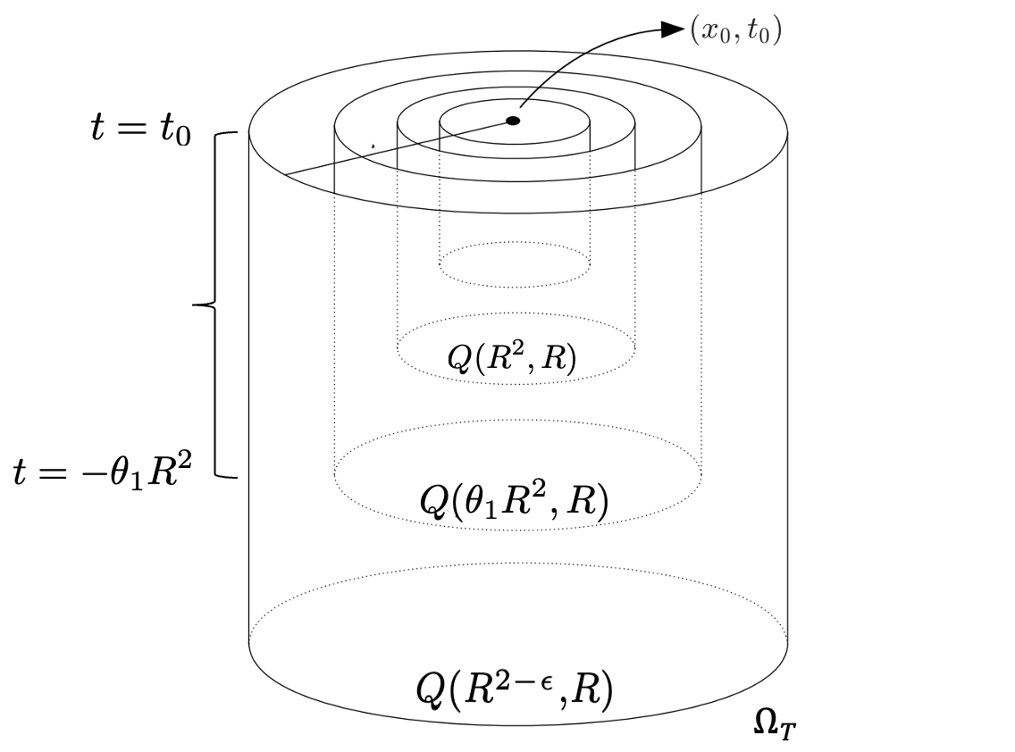
where c0c_{0} and Θ⁡(⋅)\Theta(\cdot) are specified by assumption 𝐒𝟐\mathbf{S2}. It is noteworthy to observe that the time length of the cylinder is scaled by the inverse of the lower bound on the saturation function; thus, the degeneracy is absorbed in the dimensions of the cylinder. Furthermore, the rescaled cylinder reduces to the standard parabolic cylinder associated with the heat equation if no degeneracy is present in the equation, i.e., if we fix β=0\beta=0 and c0=c1=1c_{0}=c_{1}=1 in assumption 𝐒𝟐\bf{S2}, see Figure 1 for a schematic.

Refer to caption
Figure 1. The standard parabolic cylinder Q⁡(R2,R)Q(R^{2},R) contained in the rescaled cylinder Q⁡(θ1​R2,R)Q(\theta_{1}R^{2},R).

As 0≤ρ≤10\leq\rho\leq 1 by assumption, we may fix μ−:=0\mu^{-}:=0 and μ+:=1\mu^{+}:=1 throughout for convenience. We enforce that

Q⁡(θ1​R2,R)⊂Q⁡(R2−ϵ,R)⊂ΩT,Q(\theta_{1}R^{2},R)\subset Q(R^{2-\epsilon},R)\subset\Omega_{T},

entailing

(2.7) Rϵ≤1θ1≤c0,R^{\epsilon}\leq\dfrac{1}{\theta_{1}}\leq c_{0},

and consequently

(2.8) ess​oscQ⁡(θ1​R2,R)⁡ρ≤ω\essosc_{Q(\theta_{1}R^{2},R)}\rho\leq\omega

which is a crucial assumption for the iteration process leading to the oscillation decay.

Remark 2.1.

If (2.7) does not hold, then it would hold that θ1−1<Rϵ\theta_{1}^{-1}<R^{\epsilon}, which implies that the oscillation ω\omega tends to zero as the radius RR does. The desired oscillation decay in such a situation is obvious.

Remark 2.2.

We will frequently encounter quantities of the form Ci​Rb^i​N​κ​ω−biC_{i}R^{\hat{b}_{i}N\kappa}\omega^{-b_{i}} for a fixed κ>1\kappa>1 and some constants Ci,bj>1C_{i},b_{j}>1, b^j>0\hat{b}_{j}>0 that can be determined a priori from the data of the problem. We may enforce, without loss of generality, that

Ci​Rb^i​N​κ​ω−bi≤1.C_{i}R^{\hat{b}_{i}N\kappa}\omega^{-b_{i}}\leq 1.

If not, we have that ω<C​Rϵ0\omega<CR^{\epsilon_{0}}, where C:=(maxi⁡Ci)1/minj⁡bjC:=\left(\max_{i}C_{i}\right)^{1/\min_{j}b_{j}} and ϵ0:=minj⁡b^j​N​κ/maxj⁡bj\epsilon_{0}:=\min_{j}\hat{b}_{j}N\kappa/\max_{j}b_{j}, in which case the oscillation decay is obvious.

Remark 2.3.

Future calculations reveal the explicit values of the constants in the previous remark: κ=1+4/N\kappa=1+4/N, minj⁡b^j=2/(N+4)\min_{j}\hat{b}_{j}=2/(N+4), minj⁡bj=β+1\min_{j}b_{j}=\beta+1, maxj⁡bj=2​(β+1)\max_{j}b_{j}=2(\beta+1), and maxi⁡Ci=max⁡{c0−2,1}​24​β+2​s∗\max_{i}C_{i}=\max\{c_{0}^{-2},1\}2^{4\beta+2s_{*}} where s∗≥4s_{*}\geq 4 is some fixed finite number that depends on the data.

2.3. Notations and auxiliary results

Given S⊂ℝNS\subset\mathbb{R}^{N} measurable, we write |S||S| to denote the Lebesgue measure of SS in ℝN\mathbb{R}^{N}. We denote by CC a generic positive constant or C⁡(X)C(X) to emphasize the dependence of CC on XX.

For a function v:Ω→ℝv:\Omega\to\mathbb{R} and two real numbers k1<k0k_{1}<k_{0}, we will adopt the following notation

[k1<v<k0]:={x∈Ω:k1<v(x)<k0},[k_{1}<v<k_{0}]:=\{x\in\Omega:k_{1}<v(x)<k_{0}\},

and the usual conventions

v+=max⁡{v,0},v−:=max⁡{−v,0}.v_{+}=\max\{v,0\},\ \ \ \ \ v_{-}:=\max\{-v,0\}.

Given constants a,b,ca,b,c, with a>c>0a>c>0, we will employ the following nonnegative logarithmic function:

ψ{a,b,c}±​(s)\displaystyle\psi^{\pm}_{\{a,b,c\}}(s) :=(log⁡a(a+c)−(s−b)±)+\displaystyle:=\left(\log\dfrac{a}{(a+c)-(s-b)_{\pm}}\right)_{+}
(2.9) ={log⁡a(a+c)±(b−s)if ​b±c≶s≶b±(a+c),0if ​s  ≤ ≥ b±c,\displaystyle=\begin{cases}\log\dfrac{a}{(a+c)\pm(b-s)}&\text{if }b\pm c\lessgtr s\lessgtr b\pm(a+c),\\ 0&\text{if }s\mathrel{\lx@scalerel@obj{\hbox{\hskip 4.09721pt\hskip-4.09721pt\hbox{$\hbox{\hskip 4.09721pt\hskip 0.0pt\hbox{$$}\hskip 0.0pt\hskip-4.09721pt\raisebox{1.59659pt}{\hbox{$\scriptscriptstyle\leq$}}\hskip-4.09721pt\hskip 4.09721pt}$}\hskip-4.09721pt\hskip-4.09721pt\raisebox{-5.19318pt}{\hbox{$\scriptscriptstyle\geq$}}\hskip-4.09721pt\hskip 4.09721pt}}}b\pm c,\end{cases}

whose first derivative is

(2.10) (ψ{a,b,c}±)′​(s)\displaystyle\left(\psi^{\pm}_{\{a,b,c\}}\right)^{\prime}(s) ={1(b−s)±(a+c)if ​b±c≶s≶b±(a+c),0if ​s≶b±c,\displaystyle=\begin{cases}\dfrac{1}{(b-s)\pm(a+c)}&\text{if }b\pm c\lessgtr s\lessgtr b\pm(a+c),\\ 0&\text{if }s\lessgtr b\pm c,\end{cases}

with (ψ±)′  ≥ ≤ 0(\psi^{\pm})^{\prime}\mathrel{\lx@scalerel@obj{\hbox{\hskip 4.09721pt\hskip-4.09721pt\hbox{$\hbox{\hskip 4.09721pt\hskip 0.0pt\hbox{$$}\hskip 0.0pt\hskip-4.09721pt\raisebox{1.59659pt}{\hbox{$\scriptscriptstyle\geq$}}\hskip-4.09721pt\hskip 4.09721pt}$}\hskip-4.09721pt\hskip-4.09721pt\raisebox{-5.19318pt}{\hbox{$\scriptscriptstyle\leq$}}\hskip-4.09721pt\hskip 4.09721pt}}}0 for which the following (in)equalities hold [17]:

(2.11a) ψ±\displaystyle\psi^{\pm} ≤log⁡ac,\displaystyle\leq\log\dfrac{a}{c},
(2.11b) (ψ±)′\displaystyle(\psi^{\pm})^{\prime} ≤1c,\displaystyle\leq\dfrac{1}{c},
(2.11c) (ψ±)′′\displaystyle(\psi^{\pm})^{\prime\prime} =[(ψ±)′]2.\displaystyle=[(\psi^{\pm})^{\prime}]^{2}.

For k∈ℝk\in\mathbb{R}, t,r>0t,r>0, and a function ρ=ρ⁡(x,t)\rho=\rho(x,t), we will work with truncated versions of ρ\rho, that is (ρ−k)±(\rho-k)_{\pm}, satisfying

(2.12) Hρ,k±:=ess​supQ⁡(t,r)⁡(ρ−k)±≤δ0,H_{\rho,k}^{\pm}:=\esssup_{Q(t,r)}\ (\rho-k)_{\pm}\leq\delta_{0},

for some determined δ0>0\delta_{0}>0; and the sets

(2.13) Ak,r±​(s):={x∈Br​(x0):±ρ⁡(x,s)>±k}.A_{k,r}^{\pm}(s):=\{x\in B_{r}(x_{0}):\pm\rho(x,s)>\pm k\}.

We recall the parabolic Sobolev space

V2​(ΩT):=L∞​(0,T,L2​(Ω))∩L2​(0,T,H1​(Ω)),V^{2}(\Omega_{T}):=L^{\infty}(0,T;L^{2}(\Omega))\cap L^{2}(0,T;H^{1}(\Omega)),

endowed with the norm

(2.14) ‖v‖V2​(ΩT)2:=ess​sup0<t<T⁡‖v‖L2​(Ω)2+‖∇v‖L2​(ΩT)2.\|v\|^{2}_{V^{2}(\Omega_{T})}:=\esssup_{0<t<T}\|v\|^{2}_{L^{2}(\Omega)}+\|\nabla v\|^{2}_{L^{2}(\Omega_{T})}.

In addition to the constant σmax\sigma_{\textnormal{max}} given in assumption 𝐒𝟏\bf{S1}, we fix the following frequent quantity

(2.15) Λ:=2⋅max⁡{‖∇V‖L∞​(Ω),‖∇W‖L∞​(Ω)},\Lambda:=2\cdot\max\{\|\nabla V\|_{L^{\infty}(\Omega)},\|\nabla W\|_{L^{\infty}(\Omega)}\},

which is finite by assumptions 𝐕\bf{V} and 𝐖\bf{W}. We employ the following convergence result quoted from [17, Sec. 4.2 of Ch. I].

Lemma 2.1 (Fast geometric convergence).

Let {Yn}\{Y_{n}\} and {Zn}\{Z_{n}\}, for n=0,1,2,…n=0,1,2,\dots, be sequences of positive numbers satisfying the recursive inequalities

{Yn+1≤C​bn​(Yn1+υ+Ynυ​Zn1+κ),Zn+1≤C​bn​(Yn+Zn1+κ),\begin{cases}Y_{n+1}\leq Cb^{n}\left(Y_{n}^{1+\upsilon}+Y_{n}^{\upsilon}Z_{n}^{1+\kappa}\right),\\ Z_{n+1}\leq Cb^{n}\left(Y_{n}+Z_{n}^{1+\kappa}\right),\end{cases}

where C,b>1C,b>1 and κ,υ>0\kappa,\upsilon>0 are given numbers. If

Y0+Z01+κ≤(2​C)−1+κd​b−1+κd2,whered:=min⁡{κ,υ},Y_{0}+Z_{0}^{1+\kappa}\leq(2C)^{-\tfrac{1+\kappa}{d}}b^{-\tfrac{1+\kappa}{d^{2}}},\ \ \ \ \text{where}\ \ \ d:=\min\{\kappa,\upsilon\},

then {Yn}\{Y_{n}\} and {Zn}\{Z_{n}\} tend to zero as n→∞n\to\infty.

Finally, we recall DeGiorgi’s lemma (cf. [17, Lemma 2.2 of Ch. I]).

Lemma 2.2 (DeGiorgi’s isoperimetric inequality).

Let v∈W1,1​(Br​(x0))v\in W^{1,1}(B_{r}(x_{0})), where Br​(x0)⊂Ω⊂ℝNB_{r}(x_{0})\subset\Omega\subset\mathbb{R}^{N}. Let k1<k0k_{1}<k_{0} be two real numbers. Then, there exists a constant C=C⁡(N)>0C=C(N)>0 such that

(k0−k1)|v>k0|≤C(N)rN+1|v<k1|∫[k1<ρ<k0]|∇v|dx.(k_{0}-k_{1})|v>k_{0}|\leq C(N)\dfrac{r^{N+1}}{|v<k_{1}|}\int_{[k_{1}<\rho<k_{0}]}|\nabla v|dx.

2.4. Energy estimates

We shall consider two complementary cases. Given ν∈(0,1)\nu\in(0,1), to be determined depending only on the data, the weak solution ρ\rho of (1.3) satisfies either

(2.16) |{(x,t)∈Q⁡(θ1​R2,R):ρ⁡(x,t)>1−ω2}|≤ν​|Q⁡(θ1​R2,R)|,\left|\left\{(x,t)\in Q(\theta_{1}R^{2},R):\rho(x,t)>1-\dfrac{\omega}{2}\right\}\right|\leq\nu|Q(\theta_{1}R^{2},R)|,

or

(2.17) |{(x,t)∈Q⁡(θ1​R2,R):ρ⁡(x,t)<ω2}|<(1−ν)​|Q⁡(θ1​R2,R)|.\left|\left\{(x,t)\in Q(\theta_{1}R^{2},R):\rho(x,t)<\dfrac{\omega}{2}\right\}\right|<(1-\nu)|Q(\theta_{1}R^{2},R)|.

The aim is to show that in either case, decreasing the size of the parabolic cylinder of Q⁡(θ1​R2,R)Q(\theta_{1}R^{2},R) is accompanied by a reduction in the oscillation of the solution. We stress that such a reduction is controlled by a factor that does not depend on the oscillation ω\omega nor the radius RR of the parabolic cylinder.

As mentioned earlier, the intrinsic scaling approach relies on crafting particular energy estimates employed to reach desired conclusions when either (2.16) or (2.17) holds. In the following proposition, we construct a Caccioppoli-type estimate for the weak solution.

Proposition 2.1.

Let 0≤ρ≤10\leq\rho\leq 1 be a weak solution for (1.3) in ΩT\Omega_{T}. There exists constants C⁡(⋅)>0C(\cdot)>0, depending only on the data, such that for every parabolic cylinder Q⁡(τ,r)⊂ΩTQ(\tau,r)\subset\Omega_{T}, every k∈ℝk\in\mathbb{R}, and every nonnegative, piecewise, smooth cutoff function ζ\zeta in Q⁡(τ,r)Q(\tau,r), there holds

ess​sup−τ<t<0∫Br×{t}\displaystyle\esssup_{-\tau<t<0}\int_{B_{r}\times\{t\}} (ρ−k)±2​ζ2​𝑑x+∬Q⁡(τ,r)σ⁡(ρ)​|∇(ρ−k)±|2​𝑑x​𝑑t\displaystyle(\rho-k)_{\pm}^{2}\zeta^{2}dx+\iint\limits_{Q(\tau,r)}\sigma(\rho)|\nabla(\rho-k)_{\pm}|^{2}dxdt
≤∫Br×{−τ}(ρ−k)±2​ζ2​𝑑x+C​∬Q⁡(τ,r)σ⁡(ρ)​(ρ−k)±2​|∇ζ|2​𝑑x​𝑑t\displaystyle\leq\int_{B_{r}\times\{-\tau\}}(\rho-k)_{\pm}^{2}\zeta^{2}dx+C\iint\limits_{Q(\tau,r)}\sigma(\rho)(\rho-k)_{\pm}^{2}|\nabla\zeta|^{2}dxdt
(2.18) +C∬Q⁡(τ,r)(ρ−k)±2ζ∂tζ+C(σmax,Λ)[∫−τ0|Ak,r±(t)|dt].\displaystyle+C\iint\limits_{Q(\tau,r)}(\rho-k)_{\pm}^{2}\zeta\partial_{t}\zeta+C(\sigma_{\textnormal{max}},\Lambda)\left[\int_{-\tau}^{0}|A_{k,r}^{\pm}(t)|dt\right].
Proof.

In the weak formulation (2.2), we take the test function ϕ=±(ρh−k)±​ζ2\phi=\pm(\rho_{h}-k)_{\pm}\zeta^{2}, and integrate in time over the range (−τ,t∘)(-\tau,t_{\circ}) for t∘∈(−τ,0)t_{\circ}\in(-\tau,0):

∬Q⁡(τ,r)∂tρh​[±(ρh−k)±​ζ2]​dx​dt⏟ℐ1+∬Q⁡(τ,r)(σ(ρ)∇ρ)h⋅∇[±(ρh−k)±ζ2]dxdt⏟ℐ2\displaystyle\underbrace{\iint\limits_{Q(\tau,r)}\partial_{t}\rho_{h}\left[\pm\left(\rho_{h}-k\right)_{\pm}\zeta^{2}\right]dxdt}_{\mathcal{I}_{1}}+\underbrace{\iint\limits_{Q(\tau,r)}(\sigma(\rho)\nabla\rho)_{h}\cdot\nabla\left[\pm\left(\rho_{h}-k\right)_{\pm}\zeta^{2}\right]dxdt}_{\mathcal{I}_{2}}
+∬Q⁡(τ,r)(ρσ(ρ))h∇[V+W∗ρh]⋅∇[±(ρh−k)±ζ2]dxdt⏟ℐ3=0.\displaystyle+\underbrace{\iint\limits_{Q(\tau,r)}(\rho\sigma(\rho))_{h}\nabla\big[V+W*\rho_{h}\big]\cdot\nabla\left[\pm\left(\rho_{h}-k\right)_{\pm}\zeta^{2}\right]dxdt}_{\mathcal{I}_{3}}=0.

We analyze each term separately. Integrating by parts and passing to the limit as h→0h\to 0 (see [32, Lemma 2.1.2]), we get

ℐ1\displaystyle\mathcal{I}_{1} =12​∬Q⁡(τ,r)∂t[(ρh−k)±2]​ζ2​𝑑x​𝑑t\displaystyle=\dfrac{1}{2}\iint\limits_{Q(\tau,r)}\partial_{t}\left[(\rho_{h}-k)_{\pm}^{2}\right]\zeta^{2}dxdt
→12​∫Br×{t∘}(ρ−k)±2​ζ2​𝑑x−12​∫Br×{−τ}(ρ−k)±2​ζ2​𝑑x\displaystyle\to\dfrac{1}{2}\int_{B_{r}\times\{t_{\circ}\}}(\rho-k)_{\pm}^{2}\zeta^{2}dx-\dfrac{1}{2}\int_{B_{r}\times\{-\tau\}}(\rho-k)_{\pm}^{2}\zeta^{2}dx
(2.19) −∬Q⁡(τ,r)(ρ−k)±2ζ∂tζdxdt.\displaystyle-\iint\limits_{Q(\tau,r)}(\rho-k)_{\pm}^{2}\zeta\partial_{t}\zeta dxdt.

As to the second and third terms, we again pass to the limit h→0h\to 0 and estimate from below:

ℐ2\displaystyle\mathcal{I}_{2} →±∬Q⁡(τ,r)σ(ρ)∇ρ⋅∇(ρ−k)±ζ2dxdt±2∬Q⁡(τ,r)σ(ρ)∇ρ(ρ−k)±ζ⋅∇ζdxdt\displaystyle\to\pm\iint\limits_{Q(\tau,r)}\sigma(\rho)\nabla\rho\cdot\nabla(\rho-k)_{\pm}\zeta^{2}dxdt\pm 2\iint\limits_{Q(\tau,r)}\sigma(\rho)\nabla\rho(\rho-k)_{\pm}\zeta\cdot\nabla\zeta dxdt
≥(1−ε1)​∬Q⁡(τ,r)σ⁡(ρ)​|∇(ρ−k)±|2​ζ2​𝑑x​𝑑t−1ε1​∬Q⁡(τ,r)σ⁡(ρ)​(ρ−k)±2​|∇ζ|2​𝑑x​𝑑t,\displaystyle\geq(1-\varepsilon_{1})\iint\limits_{Q(\tau,r)}\sigma(\rho)|\nabla(\rho-k)_{\pm}|^{2}\zeta^{2}dxdt-\dfrac{1}{\varepsilon_{1}}\iint\limits_{Q(\tau,r)}\sigma(\rho)(\rho-k)^{2}_{\pm}|\nabla\zeta|^{2}dxdt,

where we have applied Young’s inequality to the second term in ℐ2\mathcal{I}_{2}:

|±2∬Q⁡(τ,r)σ(ρ)∇(ρ−k)±(ρ−k)±ζ⋅∇ζdxdt|\displaystyle\left|\pm 2\iint\limits_{Q(\tau,r)}\sigma(\rho)\nabla(\rho-k)_{\pm}(\rho-k)_{\pm}\zeta\cdot\nabla\zeta dxdt\right| ≤ε1​∬Q⁡(τ,r)σ⁡(ρ)​|∇(ρ−k)±|2​ζ2​𝑑x​𝑑t\displaystyle\leq\varepsilon_{1}\iint\limits_{Q(\tau,r)}\sigma(\rho)|\nabla(\rho-k)_{\pm}|^{2}\zeta^{2}dxdt
+1ε1∬Q⁡(τ,r)σ(ρ)(ρ−k)±2|∇ζ|2dxdt.\displaystyle+\dfrac{1}{\varepsilon_{1}}\iint\limits_{Q(\tau,r)}\sigma(\rho)(\rho-k)^{2}_{\pm}|\nabla\zeta|^{2}dxdt.

Likewise, recalling the quantity σmax\sigma_{\textnormal{max}} fixed in assumption 𝐒𝟏\bf{S1}, Λ\Lambda given in (2.15), and the assumption 0≤ρ≤10\leq\rho\leq 1, we estimate

|ℐ3|\displaystyle|\mathcal{I}_{3}| ≤∬Q⁡(τ,r)Λ​σ​(ρ)|∇(ρ−k)±|ζ2​𝑑x​𝑑t+2​∬Q⁡(τ,r)Λ​σ​(ρ)​(ρ−k)±​ζ​|∇ζ|​𝑑x​𝑑t\displaystyle\leq\iint\limits_{Q(\tau,r)}\Lambda\sigma(\rho)|\nabla(\rho-k)_{\pm}|\zeta^{2}dxdt+2\iint\limits_{Q(\tau,r)}\Lambda\sigma(\rho)(\rho-k)_{\pm}\zeta|\nabla\zeta|dxdt
≤12​ε2​∬Q⁡(τ,r)σ⁡(ρ)​|∇(ρ−k)±|2​ζ2​𝑑x​𝑑t+1ε3​∬Q⁡(τ,r)σ⁡(ρ)​(ρ−k)±2​|∇ζ|2​𝑑x​𝑑t\displaystyle\leq\dfrac{1}{2\varepsilon_{2}}\iint\limits_{Q(\tau,r)}\sigma(\rho)|\nabla(\rho-k)_{\pm}|^{2}\zeta^{2}dxdt+\dfrac{1}{\varepsilon_{3}}\iint\limits_{Q(\tau,r)}\sigma(\rho)(\rho-k)^{2}_{\pm}|\nabla\zeta|^{2}dxdt
+(ε22+ε3)σmaxΛ∬Q⁡(τ,r)χ{±ρ>±k}dxdt.\displaystyle+\left(\dfrac{\varepsilon_{2}}{2}+\varepsilon_{3}\right)\sigma_{\textnormal{max}}\Lambda\iint\limits_{Q(\tau,r)}\chi_{\{\pm\rho>\pm k\}}dxdt.

Choosing ε1=1/4,ε2=2\varepsilon_{1}=1/4,\varepsilon_{2}=2, ε3=1\varepsilon_{3}=1 and recalling the definition (2.13) yield

ℐ2+ℐ3\displaystyle\mathcal{I}_{2}+\mathcal{I}_{3} ≥12​∬Q⁡(τ,r)σ⁡(ρ)​|∇(ρ−k)±|2​ζ2​𝑑x​𝑑t−5​∬Q⁡(τ,r)σ⁡(ρ)​(ρ−k)+2​|∇ζ|2​𝑑x​𝑑t\displaystyle\geq\dfrac{1}{2}\iint\limits_{Q(\tau,r)}\sigma(\rho)|\nabla(\rho-k)_{\pm}|^{2}\zeta^{2}dxdt-5\iint\limits_{Q(\tau,r)}\sigma(\rho)(\rho-k)^{2}_{+}|\nabla\zeta|^{2}dxdt
(2.20) −2σmax⋅Λ[∫−τ0|Ak,r±(t)|dt].\displaystyle-2\sigma_{\textnormal{max}}\cdot\Lambda\left[\int_{-\tau}^{0}|A_{k,r}^{\pm}(t)|dt\right].

Rearranging (2.19)-(2.20) and noting that t∘∈(−τ,0)t_{\circ}\in(-\tau,0) is arbitrary yield the desired estimate. ∎

The next proposition demonstrates a logarithmic energy estimate for the weak solution. Such an estimate will be employed to expand, in time, certain claims established in parabolic subcylinders to hold in the entirety of the containing cylinder. The logarithmic function ψ±\psi^{\pm} and its properties have been listed in Section 2.3.

Proposition 2.2.

Let 0≤ρ≤10\leq\rho\leq 1 be a weak solution for (1.3) in ΩT\Omega_{T} and Hρ,k±H_{\rho,k}^{\pm} be as defined in (2.12). There exist constants c,C⁡(⋅)>0c,C(\cdot)>0, depending only on the data, such that for every parabolic cylinder Q⁡(τ,r)⊂ΩTQ(\tau,r)\subset\Omega_{T}, every k∈ℝk\in\mathbb{R}, and every nonnegative, piecewise smooth cutoff function ζ\zeta in Q⁡(τ,r)Q(\tau,r), there holds

ess​sup−τ<t<0\displaystyle\esssup_{-\tau<t<0} ∫Br×{t}[ψ±​(ρ)]2​ζ2​𝑑x≤∫Br×{−τ}[ψ±​(ρ)]2​ζ2​𝑑x\displaystyle\int_{B_{r}\times\{t\}}[\psi^{\pm}(\rho)]^{2}\zeta^{2}dx\leq\int_{B_{r}\times\{-\tau\}}[\psi^{\pm}(\rho)]^{2}\zeta^{2}dx
(2.21) +C∬Q⁡(τ,r)σ(ρ)ψ±(ρ)|∇ζ|2dxdt+C⁡(σmax,Λ)c2(1+logHρ,k±c)[∫−τ0|Ak,r±(t)|dt].\displaystyle+C\iint\limits_{Q(\tau,r)}\sigma(\rho)\psi^{\pm}(\rho)|\nabla\zeta|^{2}dxdt+\dfrac{C(\sigma_{\textnormal{max}},\Lambda)}{c^{2}}\left(1+\log\dfrac{H^{\pm}_{\rho,k}}{c}\right)\left[\int_{-\tau}^{0}|A_{k,r}^{\pm}(t)|dt\right].
Proof.

Recall the logarithmic function (2.9) and set

ψ±:=ψ{Hρ,k±,(ρ−k)±,c}±​(ρ)\psi^{\pm}:=\psi^{\pm}_{\{H_{\rho,k}^{\pm},(\rho-k)_{\pm},c\}}(\rho)

for some 0<c<Hρ,k±0<c<H_{\rho,k}^{\pm}. In (2.2), take the test function

ϕ=∂ρh[ψ±​(ρh)]2​ζ2=2​ψ±​(ψ±)′​ζ2,\phi=\partial_{\rho_{h}}[\psi^{\pm}(\rho_{h})]^{2}\zeta^{2}=2\psi^{\pm}(\psi^{\pm})^{\prime}\zeta^{2},

to obtain

∬Q⁡(τ,r)∂tρh​[2​ψ±​(ψ±)′​ζ2]​dx​dt⏟ℐ1+∬Q⁡(τ,r)(σ(ρ)∇ρ)h⋅∇[2ψ±(ψ±)′ζ2]dxdt⏟ℐ2\displaystyle\underbrace{\iint\limits_{Q(\tau,r)}\partial_{t}\rho_{h}\left[2\psi^{\pm}(\psi^{\pm})^{\prime}\zeta^{2}\right]dxdt}_{\mathcal{I}_{1}}+\underbrace{\iint\limits_{Q(\tau,r)}(\sigma(\rho)\nabla\rho)_{h}\cdot\nabla\left[2\psi^{\pm}(\psi^{\pm})^{\prime}\zeta^{2}\right]dxdt}_{\mathcal{I}_{2}}
+∬Q⁡(τ,r)(ρσ(ρ))h∇[V+W∗ρh]⋅∇[2ψ±(ψ±)′ζ2]dxdt⏟ℐ3=0.\displaystyle+\underbrace{\iint\limits_{Q(\tau,r)}(\rho\sigma(\rho))_{h}\nabla\big[V+W*\rho_{h}\big]\cdot\nabla\left[2\psi^{\pm}(\psi^{\pm})^{\prime}\zeta^{2}\right]dxdt}_{\mathcal{I}_{3}}=0.

Sending h→0h\to 0, we obtain, for any t∘∈(−τ,0)t_{\circ}\in(-\tau,0),

(2.22) ℐ1→∫Br×{t∘}[ψ±​(ρ)]2​ζ2​𝑑x−∫Br×{−τ}[ψ±​(ρ)]2​ζ2​𝑑x.\displaystyle\mathcal{I}_{1}\to\int_{B_{r}\times\{t_{\circ}\}}[\psi^{\pm}(\rho)]^{2}\zeta^{2}dx-\int_{B_{r}\times\{-\tau\}}[\psi^{\pm}(\rho)]^{2}\zeta^{2}dx.

Considering the second term, take h→0h\to 0 and apply Young’s inequality to obtain

ℐ2\displaystyle\mathcal{I}_{2} →2∬Q⁡(τ,r)σ(ρ)∇ρ⋅∇ρ(1+ψ±)[(ψ±)′]2ζ2dxdt+4∬Q⁡(τ,r)σ(ρ)∇ρ⋅∇ζψ±(ψ±)′ζdxdt\displaystyle\to 2\iint\limits_{Q(\tau,r)}\sigma(\rho)\nabla\rho\cdot\nabla\rho(1+\psi^{\pm})[(\psi^{\pm})^{\prime}]^{2}\zeta^{2}dxdt+4\iint\limits_{Q(\tau,r)}\sigma(\rho)\nabla\rho\cdot\nabla\zeta\psi^{\pm}(\psi^{\pm})^{\prime}\zeta dxdt
≥2​∬Q⁡(τ,r)σ⁡(ρ)​|∇ρ|2​(1+ψ±)​[(ψ±)′]2​ζ2​𝑑x​𝑑t\displaystyle\geq 2\iint\limits_{Q(\tau,r)}\sigma(\rho)|\nabla\rho|^{2}(1+\psi^{\pm})[(\psi^{\pm})^{\prime}]^{2}\zeta^{2}dxdt
−2∬Q⁡(τ,r)ε1σ(ρ)|∇ζ|2dxdt−2∬Q⁡(τ,r)1ε1σ(ρ)|∇ρ|2[ψ±]2[(ψ±)′]2ζ2dxdt.\displaystyle-2\iint\limits_{Q(\tau,r)}\varepsilon_{1}\sigma(\rho)|\nabla\zeta|^{2}dxdt-2\iint\limits_{Q(\tau,r)}\dfrac{1}{\varepsilon_{1}}\sigma(\rho)|\nabla\rho|^{2}[\psi^{\pm}]^{2}[(\psi^{\pm})^{\prime}]^{2}\zeta^{2}dxdt.

The third term is estimated as

|ℐ3|\displaystyle|\mathcal{I}_{3}| ≤2​∬Q⁡(τ,r)Λ​σ​(ρ)|∇ρ|(1+ψ±)​[(ψ±)′]2​ζ2​𝑑x​𝑑t+4​∬Q⁡(τ,r)Λ​σ​(ρ)​|∇ζ|​ψ±​(ψ±)′​ζ​𝑑x​𝑑t\displaystyle\leq 2\iint\limits_{Q(\tau,r)}\Lambda\sigma(\rho)|\nabla\rho|(1+\psi^{\pm})[(\psi^{\pm})^{\prime}]^{2}\zeta^{2}dxdt+4\iint\limits_{Q(\tau,r)}\Lambda\sigma(\rho)|\nabla\zeta|\psi^{\pm}(\psi^{\pm})^{\prime}\zeta dxdt
≤∬Q⁡(τ,r)σ⁡(ρ)​(ε2​|∇ρ|2+1ε2​Λ2)​(1+ψ±)​[(ψ±)′]2​ζ2​𝑑x​𝑑t\displaystyle\leq\iint\limits_{Q(\tau,r)}\sigma(\rho)\left(\varepsilon_{2}|\nabla\rho|^{2}+\dfrac{1}{\varepsilon_{2}}\Lambda^{2}\right)(1+\psi^{\pm})[(\psi^{\pm})^{\prime}]^{2}\zeta^{2}dxdt
+2∬Q⁡(τ,r)σ(ρ)(ε3|∇ζ|2+1ε3Λ2[ψ±(ψ±)′]2ζ2)dxdt.\displaystyle+2\iint\limits_{Q(\tau,r)}\sigma(\rho)\left(\varepsilon_{3}|\nabla\zeta|^{2}+\dfrac{1}{\varepsilon_{3}}\Lambda^{2}[\psi^{\pm}(\psi^{\pm})^{\prime}]^{2}\zeta^{2}\right)dxdt.

Choosing ε1=2​ψ±\varepsilon_{1}=2\psi^{\pm}, ε2=1\varepsilon_{2}=1, ε3=ψ±\varepsilon_{3}=\psi^{\pm} and noting ψ±≤(1+ψ±)\psi^{\pm}\leq(1+\psi^{\pm}), we obtain the lower bound

ℐ2+ℐ3\displaystyle\mathcal{I}_{2}+\mathcal{I}_{3} ≥−6∬Q⁡(τ,r)σ(ρ)ψ±(ρ)|∇ζ|2dxdt\displaystyle\geq-6\iint\limits_{Q(\tau,r)}\sigma(\rho)\psi^{\pm}(\rho)|\nabla\zeta|^{2}dxdt
(2.23) −3​σmax⋅Λ2c2​(1+log⁡Hρ,k±c)​[∫−τ0|Ak,r±​(t)|​𝑑t],\displaystyle-3\dfrac{\sigma_{\textnormal{max}}\cdot\Lambda^{2}}{c^{2}}\left(1+\log\dfrac{H^{\pm}_{\rho,k}}{c}\right)\left[\int_{-\tau}^{0}|A_{k,r}^{\pm}(t)|dt\right],

where we have used the estimates (2.11). Collecting (2.22)-(2.23) yield the desired estimate. ∎

2.5. Behavior near the saturation value

We begin by assuming that (2.16) holds in the parabolic cylinder Q⁡(θ1​R2,R)Q(\theta_{1}R^{2},R). The aim of the following proposition is to show that the value of the solution ρ\rho is below the saturation value in a smaller parabolic cylinder, along with determining ν\nu. The oscillation reduction then follows immediately.

Proposition 2.3.

There exists a number ν∈(0,1)\nu\in(0,1), depending only on the data, such that if (2.16) holds, then,

(2.24) ρ⁡(x,t)<1−ω4 a.e. in (x,t)∈Q⁡(θ1​(R2)2,R2).\rho(x,t)<1-\dfrac{\omega}{4}\ \ \ \text{ a.e. in }\ \ (x,t)\in Q\bigg(\theta_{1}\left(\frac{R}{2}\right)^{2},\frac{R}{2}\bigg).
Proof.

We shall work with the quantity ρω:=min⁡{ρ,1−ω4}\rho_{\omega}:=\min\{\rho,1-\frac{\omega}{4}\} and proceed to construct an energy estimate for a truncated version of it. Define, for n=0,1,2,…n=0,1,2,\dots, the two sequences

Rn\displaystyle R_{n} =R2+R2n+1,\displaystyle=\dfrac{R}{2}+\dfrac{R}{2^{n+1}},
kn\displaystyle k_{n} =1−ω4−ω2n+2.\displaystyle=1-\dfrac{\omega}{4}-\dfrac{\omega}{2^{n+2}}.

Construct a family of nested and shrinking parabolic cylinders Qn1:=Q⁡(θ1​Rn2,Rn)Q_{n}^{1}:=Q(\theta_{1}R^{2}_{n},R_{n}) along with the corresponding cutoff functions 0≤ζn≤10\leq\zeta_{n}\leq 1 in Qn1Q_{n}^{1} satisfying:

(2.25) {ζn≡1in​Qn+11,ζn≡0on​∂pQn1,0≤∂tζn≤22​(n+2)θ1​R2,|∇ζn|≤2n+2R,|Δζn|≤22​(n+2)R2,\begin{cases}\zeta_{n}\equiv 1\ \ \ \ \ \text{in}\ Q_{n+1}^{1},\\ \zeta_{n}\equiv 0\ \ \ \ \ \text{on}\ \partial_{p}Q_{n}^{1},\\ 0\leq\partial_{t}\zeta_{n}\leq\dfrac{2^{2(n+2)}}{\theta_{1}R^{2}},\ \ \ |\nabla\zeta_{n}|\leq\dfrac{2^{n+2}}{R},\ \ |\Delta\zeta_{n}|\leq\dfrac{2^{2(n+2)}}{R^{2}},\end{cases}

where ∂pQn1\partial_{p}Q_{n}^{1} denotes the parabolic boundary of Qn1Q^{1}_{n}. In (2.2), take

ϕ:=((ρω)h−kn)+​ζn2,\phi:=\left((\rho_{\omega})_{h}-k_{n}\right)_{+}\zeta_{n}^{2},

and integrate over the time interval (−θ1​Rn2,t∘)(-\theta_{1}R^{2}_{n},t_{\circ}) for t∘∈(−θ1​Rn2,0)t_{\circ}\in(-\theta_{1}R^{2}_{n},0):

∬Qn1∂tρh​[((ρω)h−kn)+​ζn2]​dx​dt⏟ℐ1+∬Qn1(σ(ρ)∇ρ)h⋅∇[((ρω)h−kn)+ζn2]dxdt⏟ℐ2\displaystyle\underbrace{\iint\limits_{Q_{n}^{1}}\partial_{t}\rho_{h}\left[\left((\rho_{\omega})_{h}-k_{n}\right)_{+}\zeta_{n}^{2}\right]dxdt}_{\mathcal{I}_{1}}+\underbrace{\iint\limits_{Q_{n}^{1}}(\sigma(\rho)\nabla\rho)_{h}\cdot\nabla\left[\left((\rho_{\omega})_{h}-k_{n}\right)_{+}\zeta_{n}^{2}\right]dxdt}_{\mathcal{I}_{2}}
(2.26) +∬Qn1(ρσ(ρ))h∇[V+W∗ρh]⋅∇[((ρω)h−kn)+ζn2]dxdt⏟ℐ3=0.\displaystyle+\underbrace{\iint\limits_{Q_{n}^{1}}(\rho\sigma(\rho))_{h}\nabla\big[V+W*\rho_{h}\big]\cdot\nabla\big[\left((\rho_{\omega})_{h}-k_{n}\right)_{+}\zeta_{n}^{2}\big]dxdt}_{\mathcal{I}_{3}}=0.

Observe that (ρω−kn)+(\rho_{\omega}-k_{n})_{+} is nonzero on the set {kn<ρ}\{k_{n}<\rho\}. Specifically, if ρω=ρ<1−ω4\rho_{\omega}=\rho<1-\frac{\omega}{4},

(2.27) (ρω−kn)+=(ρ−kn)+≤ω2n+2≤ω4.(\rho_{\omega}-k_{n})_{+}=(\rho-k_{n})_{+}\leq\dfrac{\omega}{2^{n+2}}\leq\dfrac{\omega}{4}.

On the other hand, if ρ≥1−ω4=ρω>kn\rho\geq 1-\frac{\omega}{4}=\rho_{\omega}>k_{n}, then

(2.28) (ρω−kn)+=ω2n+2≤ω4.(\rho_{\omega}-k_{n})_{+}=\dfrac{\omega}{2^{n+2}}\leq\dfrac{\omega}{4}.

Moreover, notice that |∇(ρω−kn)+|≠0|\nabla(\rho_{\omega}-k_{n})_{+}|\neq 0 on the set {kn<ρ<1−ω4}\{k_{n}<\rho<1-\frac{\omega}{4}\}. With these observations, we proceed to estimate each term in (2.26). Firstly, we have

ℐ1\displaystyle\mathcal{I}_{1} =∬Qn1∂tρh[((ρω)h−kn)+ζn2]χ{(ρw)h=ρh}dxdt\displaystyle=\iint\limits_{Q_{n}^{1}}\partial_{t}\rho_{h}\left[\left((\rho_{\omega})_{h}-k_{n}\right)_{+}\zeta_{n}^{2}\right]\chi_{\left\{(\rho_{w})_{h}=\rho_{h}\right\}}dxdt
+∬Qn1∂tρh[((ρω)h−kn)+ζn2]χ{(ρw)h=1−ω4}dxdt\displaystyle+\iint\limits_{Q_{n}^{1}}\partial_{t}\rho_{h}\left[\left((\rho_{\omega})_{h}-k_{n}\right)_{+}\zeta_{n}^{2}\right]\chi_{\left\{(\rho_{w})_{h}=1-\frac{\omega}{4}\right\}}dxdt
=12​∬Qn1∂t[((ρω)h−kn)+2]​ζn2​𝑑x​𝑑t+(ω2n+2)​∬Qn1∂t[(ρh−[1−ω4])+]​ζn2​𝑑x​𝑑t.\displaystyle=\dfrac{1}{2}\iint\limits_{Q_{n}^{1}}\partial_{t}\left[\left((\rho_{\omega})_{h}-k_{n}\right)_{+}^{2}\right]\zeta_{n}^{2}dxdt+\left(\dfrac{\omega}{2^{n+2}}\right)\iint\limits_{Q_{n}^{1}}\partial_{t}\left[\left(\rho_{h}-\Big[1-\dfrac{\omega}{4}\Big]\right)_{+}\right]\zeta_{n}^{2}dxdt.

Next, we integrate by parts with respect to time, send h→0h\to 0, and use (2.25) to obtain

ℐ1\displaystyle\mathcal{I}_{1} →12​∫Bn×{t∘}(ρω−kn)+2​ζn2​𝑑x−∬Qn1(ρω−kn)+2​ζn​∂tζn​𝑑x​𝑑t\displaystyle\to\dfrac{1}{2}\int_{B_{n}\times\{t_{\circ}\}}(\rho_{\omega}-k_{n})_{+}^{2}\zeta_{n}^{2}dx-\iint\limits_{Q_{n}^{1}}(\rho_{\omega}-k_{n})_{+}^{2}\zeta_{n}\partial_{t}\zeta_{n}dxdt
+(ω2n+2)∫Bn×{t∘}(ρ−[1−ω4])+ζn2dx\displaystyle+\left(\dfrac{\omega}{2^{n+2}}\right)\int_{B_{n}\times\{t_{\circ}\}}\left(\rho-\Big[1-\dfrac{\omega}{4}\Big]\right)_{+}\zeta_{n}^{2}dx
−2(ω2n+2)∬Qn1(ρ−[1−ω4])+ζn∂tζndxdt\displaystyle-2\left(\dfrac{\omega}{2^{n+2}}\right)\iint\limits_{Q_{n}^{1}}\left(\rho-\Big[1-\dfrac{\omega}{4}\Big]\right)_{+}\zeta_{n}\partial_{t}\zeta_{n}dxdt
(2.29) ≥12∫Bn×{t∘}(ρω−kn)+2ζn2dx−3(ω4)222​(n+2)θ1​R2∬Qn1χ{ρω>kn}dxdt,\displaystyle\geq\dfrac{1}{2}\int_{B_{n}\times\{t_{\circ}\}}(\rho_{\omega}-k_{n})_{+}^{2}\zeta_{n}^{2}dx-3\left(\dfrac{\omega}{4}\right)^{2}\dfrac{2^{2(n+2)}}{\theta_{1}R^{2}}\iint\limits_{Q_{n}^{1}}\chi_{\{\rho_{\omega}>k_{n}\}}dxdt,

where the last inequality follows from the nonnegativity of the third term. Next, we estimate ℐ2\mathcal{I}_{2} in (2.26). Passing to the limit h→0h\to 0 and noting where ∇(ρω−kn)+\nabla\left(\rho_{\omega}-k_{n}\right)_{+} is nonzero yield

ℐ2\displaystyle\mathcal{I}_{2} →∬Qn1σ(ρ)∇ρ⋅∇[(ρω−kn)+ζn2]dxdt\displaystyle\to\iint\limits_{Q_{n}^{1}}\sigma(\rho)\nabla\rho\cdot\nabla\left[\left(\rho_{\omega}-k_{n}\right)_{+}\zeta_{n}^{2}\right]dxdt
=∬Qn1σ(ρ)∇ρ⋅∇[(ρω−kn)+ζn2]χ{ρw=ρ}dxdt\displaystyle=\iint\limits_{Q_{n}^{1}}\sigma(\rho)\nabla\rho\cdot\nabla\left[\left(\rho_{\omega}-k_{n}\right)_{+}\zeta_{n}^{2}\right]\chi_{\left\{\rho_{w}=\rho\right\}}dxdt
+∬Qn1σ(ρ)∇ρ⋅∇[(ρω−kn)+ζn2]χ{ρw=1−ω4}dxdt\displaystyle+\iint\limits_{Q_{n}^{1}}\sigma(\rho)\nabla\rho\cdot\nabla\left[\left(\rho_{\omega}-k_{n}\right)_{+}\zeta_{n}^{2}\right]\chi_{\left\{\rho_{w}=1-\frac{\omega}{4}\right\}}dxdt
=∬Qn1σ⁡(ρω)​|∇(ρω−kn)+|2​ζn2​𝑑x​𝑑t\displaystyle=\iint\limits_{Q_{n}^{1}}\sigma(\rho_{\omega})|\nabla\left(\rho_{\omega}-k_{n}\right)_{+}|^{2}\zeta_{n}^{2}dxdt
+2∬Qn1σ(ρω)∇(ρω−kn)+⋅∇ζnζn(ρω−kn)+dxdt\displaystyle+2\iint\limits_{Q_{n}^{1}}\sigma(\rho_{\omega})\nabla\left(\rho_{\omega}-k_{n}\right)_{+}\cdot\nabla\zeta_{n}\zeta_{n}\left(\rho_{\omega}-k_{n}\right)_{+}dxdt
(2.30) +2(ω2n+2)∬Qn1σ(ρ)∇ρ⋅∇ζnζnχ{ρ≥1−ω4}dxdt.\displaystyle+2\left(\dfrac{\omega}{2^{n+2}}\right)\iint\limits_{Q_{n}^{1}}\sigma(\rho)\nabla\rho\cdot\nabla\zeta_{n}\zeta_{n}\chi_{\{\rho\geq 1-\frac{\omega}{4}\}}dxdt.

Applying Young’s inequality to the second term on the rightmost side of the above expression

|2∬Qn1σ(ρω)∇(ρω−kn)+⋅∇ζnζn(ρω−kn)+dxdt|\displaystyle\left|2\iint\limits_{Q_{n}^{1}}\sigma(\rho_{\omega})\nabla\left(\rho_{\omega}-k_{n}\right)_{+}\cdot\nabla\zeta_{n}\zeta_{n}\left(\rho_{\omega}-k_{n}\right)_{+}dxdt\right|
≤14​∬Qn1σ⁡(ρω)​|∇(ρω−kn)+|2​ζn2​𝑑x​𝑑t+4​∬Qn1σ⁡(ρω)​(ρω−kn)+2​|∇ζn|2​𝑑x​𝑑t.\displaystyle\leq\dfrac{1}{4}\iint\limits_{Q_{n}^{1}}\sigma(\rho_{\omega})|\nabla\left(\rho_{\omega}-k_{n}\right)_{+}|^{2}\zeta_{n}^{2}dxdt+4\iint\limits_{Q_{n}^{1}}\sigma(\rho_{\omega})\left(\rho_{\omega}-k_{n}\right)^{2}_{+}|\nabla\zeta_{n}|^{2}dxdt.

We arrive at the lower bound

ℐ2\displaystyle\mathcal{I}_{2} ≥34​∬Qn1σ⁡(ρω)​|∇(ρω−kn)+|2​ζn2​𝑑x​𝑑t−4​∬Qn1σ⁡(ρω)​(ρω−kn)+2​|∇ζn|2​𝑑x​𝑑t\displaystyle\geq\dfrac{3}{4}\iint\limits_{Q_{n}^{1}}\sigma(\rho_{\omega})|\nabla\left(\rho_{\omega}-k_{n}\right)_{+}|^{2}\zeta_{n}^{2}dxdt-4\iint\limits_{Q_{n}^{1}}\sigma(\rho_{\omega})\left(\rho_{\omega}-k_{n}\right)^{2}_{+}|\nabla\zeta_{n}|^{2}dxdt
(2.31) +2(ω2n+2)∬Qn1σ(ρ)∇ρ⋅∇ζnζnχ{ρ≥1−ω4}dxdt⏟ℐ2′.\displaystyle+\underbrace{2\left(\dfrac{\omega}{2^{n+2}}\right)\iint\limits_{Q_{n}^{1}}\sigma(\rho)\nabla\rho\cdot\nabla\zeta_{n}\zeta_{n}\chi_{\{\rho\geq 1-\frac{\omega}{4}\}}dxdt}_{\mathcal{I}^{\prime}_{2}}.

Now, we make the following observations: on the set {1−ω2≤kn<ρω=ρ<1−ω4}\{1-\frac{\omega}{2}\leq k_{n}<\rho_{\omega}=\rho<1-\frac{\omega}{4}\}, we have by assumption 𝐒𝟐\mathbf{S2}

σ⁡(ρ)\displaystyle\sigma(\rho) ≥c0​Θ​(1−ρ)≥c0​Θ​(1−[1−ω4])=1θ1,\displaystyle\geq c_{0}\Theta\left(1-\rho\right)\geq c_{0}\Theta\left(1-\Big[1-\dfrac{\omega}{4}\Big]\right)=\dfrac{1}{\theta_{1}},
σ⁡(ρ)\displaystyle\sigma(\rho) ≤c1​Θ​(1−ρ)≤c1​Θ​(1−[1−ω2])≤2β​c1c0​1θ1,\displaystyle\leq c_{1}\Theta\left(1-\rho\right)\leq c_{1}\Theta\left(1-\Big[1-\dfrac{\omega}{2}\Big]\right)\leq 2^{\beta}\dfrac{c_{1}}{c_{0}}\dfrac{1}{\theta_{1}},

which, along with (2.25) and (2.27), allow us to estimate the first two terms on the rightmost side of (2.31) from below. As to the third term, we introduce

Σ+​(ρ):=[∫1−ω4ρσ⁡(s)​𝑑s]+,\Sigma_{+}(\rho):=\left[\int_{1-\frac{\omega}{4}}^{\rho}\sigma(s)ds\right]_{+},

and notice that on the set {1≥ρ≥1−ω4}\{1\geq\rho\geq 1-\frac{\omega}{4}\}, we have again by assumption 𝐒𝟐\mathbf{S2},

(2.32) Σ+​(ρ)\displaystyle\Sigma_{+}(\rho) ≤c1​Θ​(1−[1−ω4])​(1−[1−ω4])=c1c0​1θ1​(ω4).\displaystyle\leq c_{1}\Theta\left(1-\Big[1-\dfrac{\omega}{4}\Big]\right)\left(1-\Big[1-\dfrac{\omega}{4}\Big]\right)=\dfrac{c_{1}}{c_{0}}\dfrac{1}{\theta_{1}}\left(\dfrac{\omega}{4}\right).

Utilizing this estimate, integration by parts, and use of (2.25) and (2.28), the third term on the rightmost side of (2.31) is estimated as follows

|ℐ2′|\displaystyle\left|\mathcal{I}^{\prime}_{2}\right| ≤|2(ω2n+2)∬Qn1∇Σ+(ρ)⋅∇ζnζndxdt|\displaystyle\leq\left|2\left(\dfrac{\omega}{2^{n+2}}\right)\iint\limits_{Q_{n}^{1}}\nabla\Sigma_{+}(\rho)\cdot\nabla\zeta_{n}\zeta_{n}dxdt\right|
=|−2(ω2n+2)∬Qn1Σ+(ρ)(ζn|Δζn|+|∇ζn|2)dxdt|\displaystyle=\left|-2\left(\dfrac{\omega}{2^{n+2}}\right)\iint\limits_{Q_{n}^{1}}\Sigma_{+}(\rho)\left(\zeta_{n}|\Delta\zeta_{n}|+|\nabla\zeta_{n}|^{2}\right)dxdt\right|
≤4c1c01θ1(ω4)2(22​(n+2)R2)∬Qn1χ{ρω>kn}dxdt.\displaystyle\leq 4\dfrac{c_{1}}{c_{0}}\dfrac{1}{\theta_{1}}\left(\dfrac{\omega}{4}\right)^{2}\bigg(\dfrac{2^{2(n+2)}}{R^{2}}\bigg)\iint\limits_{Q_{n}^{1}}\chi_{\{\rho_{\omega}>k_{n}\}}dxdt.

Combining the preceding estimates, we arrive at

(2.33) ℐ2\displaystyle\mathcal{I}_{2} ≥341θ1∬Qn1|∇(ρω−kn)+|2ζn2dxdt−4(1+2β)c1c0(ω4)2(22​(n+2)θ1​R2)∬Qn1χ{ρω>kn}dxdt.\displaystyle\geq\dfrac{3}{4}\dfrac{1}{\theta_{1}}\iint\limits_{Q_{n}^{1}}|\nabla\left(\rho_{\omega}-k_{n}\right)_{+}|^{2}\zeta_{n}^{2}dxdt-4(1+2^{\beta})\dfrac{c_{1}}{c_{0}}\left(\dfrac{\omega}{4}\right)^{2}\bigg(\dfrac{2^{2(n+2)}}{\theta_{1}R^{2}}\bigg)\iint\limits_{Q_{n}^{1}}\chi_{\{\rho_{\omega}>k_{n}\}}dxdt.

As to ℐ3\mathcal{I}_{3} in (2.26), upon letting h→0h\to 0, applying Young’s inequality, we obtain

|ℐ3|\displaystyle|\mathcal{I}_{3}| ≤σmax​Λ2​ε1​∬Qn1|∇(ρω−kn)+|2​ζn2​𝑑x​𝑑t+σmax​Λε2​∬Qn1(ρω−kn)+2​|∇ζn|2​𝑑x​𝑑t\displaystyle\leq\dfrac{\sigma_{\textnormal{max}}\Lambda}{2\varepsilon_{1}}\iint\limits_{Q_{n}^{1}}|\nabla\left(\rho_{\omega}-k_{n}\right)_{+}|^{2}\zeta_{n}^{2}dxdt+\dfrac{\sigma_{\textnormal{max}}\Lambda}{\varepsilon_{2}}\iint\limits_{Q_{n}^{1}}\left(\rho_{\omega}-k_{n}\right)^{2}_{+}|\nabla\zeta_{n}|^{2}dxdt
+σmaxΛ(ε12+ε2)∬Qn1χ{ρω>kn}dxdt\displaystyle+\sigma_{\textnormal{max}}\Lambda\left(\dfrac{\varepsilon_{1}}{2}+\varepsilon_{2}\right)\iint\limits_{Q_{n}^{1}}\chi_{\{\rho_{\omega}>k_{n}\}}dxdt
≤14​1θ1​∬Qn1|∇(ρω−kn)+|2​ζn2​𝑑x​𝑑t\displaystyle\leq\dfrac{1}{4}\dfrac{1}{\theta_{1}}\iint\limits_{Q_{n}^{1}}|\nabla\left(\rho_{\omega}-k_{n}\right)_{+}|^{2}\zeta_{n}^{2}dxdt
+c1c0(ω4)2(22​(n+2)θ1​R2)∬Qn1χ{ρω>kn}dxdt\displaystyle+\dfrac{c_{1}}{c_{0}}\left(\dfrac{\omega}{4}\right)^{2}\bigg(\dfrac{2^{2(n+2)}}{\theta_{1}R^{2}}\bigg)\iint\limits_{Q_{n}^{1}}\chi_{\{\rho_{\omega}>k_{n}\}}dxdt
(2.34) +2​(σmax​Λ)2​θ1​[∫−θ1​Rn20|Akn,Rn+​(t)|​𝑑t],\displaystyle+2\left(\sigma_{\textnormal{max}}\Lambda\right)^{2}\theta_{1}\left[\int_{-\theta_{1}R^{2}_{n}}^{0}|A_{k_{n},R_{n}}^{+}(t)|dt\right],

where we chose ε1=2​θ1​σmax​Λ\varepsilon_{1}=2\theta_{1}\sigma_{\textnormal{max}}\Lambda and ε2=θ1​σmax​Λ​c0/c1\varepsilon_{2}=\theta_{1}\sigma_{\textnormal{max}}\Lambda c_{0}/c_{1}, used c0≤c1c_{0}\leq c_{1}, and defined

Akn,Rn+​(t):={x∈Bn:ρω​(x,t)>kn},A_{k_{n},R_{n}}^{+}(t):=\{x\in B_{n}:\rho_{\omega}(x,t)>k_{n}\},

with the shorthand Bn:=BRnB_{n}:=B_{R_{n}}. Subsituting (2.29),(2.33)\eqref{estim-I},\eqref{estim-II}, and (2.34) in (2.26) we arrive at the estimate

ess​sup−θ1​Rn2<t<0\displaystyle\esssup_{-\theta_{1}R_{n}^{2}<t<0} ∫Bn×{t}(ρω−kn)+2​ζn2​𝑑x+1θ1​∬Qn1|∇(ρω−kn)+|2​ζn2​𝑑x​𝑑t\displaystyle\int_{B_{n}\times\{t\}}(\rho_{\omega}-k_{n})_{+}^{2}\zeta_{n}^{2}dx+\dfrac{1}{\theta_{1}}\iint\limits_{Q_{n}^{1}}|\nabla(\rho_{\omega}-k_{n})_{+}|^{2}\zeta_{n}^{2}dxdt
≤C(β,c0,c1)(ω4)2(22​(n+2)θ1​R2)∬Qn1χ{ρω>kn}dxdt\displaystyle\leq C(\beta,c_{0},c_{1})\left(\dfrac{\omega}{4}\right)^{2}\bigg(\dfrac{2^{2(n+2)}}{\theta_{1}R^{2}}\bigg)\iint\limits_{Q_{n}^{1}}\chi_{\{\rho_{\omega}>k_{n}\}}dxdt
(2.35) +C⁡(σmax,Λ)​θ12​[1θ1​∫−θ1​Rn20|Akn,Rn+​(t)|​𝑑t].\displaystyle+C(\sigma_{\textnormal{max}},\Lambda)\theta_{1}^{2}\left[\dfrac{1}{\theta_{1}}\int_{-\theta_{1}R^{2}_{n}}^{0}|A_{k_{n},R_{n}}^{+}(t)|dt\right].

Now, we wish to write the above estimate in terms of the norm (2.14). To this end, we perform a change of the time variable by introducing

(2.36) t~=tθ1,\tilde{t}=\dfrac{t}{\theta_{1}},

such that we have

ρ~ω(⋅,t~):=ρω(⋅,t=θ1t~),andζ~n(⋅,t~):=ζn(⋅,t=θ1t~).\tilde{\rho}_{\omega}(\cdot,\tilde{t}):=\rho_{\omega}(\cdot,t=\theta_{1}\tilde{t}),\ \ \text{and}\ \ \ \tilde{\zeta}_{n}(\cdot,\tilde{t}):=\zeta_{n}(\cdot,t=\theta_{1}\tilde{t}).

Furthermore, owing to the definition of θ1\theta_{1} given in (2.6), we estimate

θ12=c0−2​24​(β+1)​ω−2​(β+1)​(ω4)2≤R−N​κ​(ω4)2,\theta_{1}^{2}=c_{0}^{-2}2^{4(\beta+1)}\omega^{-2\left(\beta+1\right)}\left(\dfrac{\omega}{4}\right)^{2}\leq R^{-N\kappa}\left(\dfrac{\omega}{4}\right)^{2},

where the inequality is due to the assumption c0−2​24​(β+1)​ω−2​(β+1)​RN​κ≤1c_{0}^{-2}2^{4(\beta+1)}\omega^{-2\left(\beta+1\right)}R^{N\kappa}\leq 1 (cf. Remark 2.2) for some κ>1\kappa>1 to be fixed momentarily. Consequently, the estimate (2.35) reads

‖(ρ~ω−kn)+​ζn~‖V2​(Qn)\displaystyle\|(\tilde{\rho}_{\omega}-k_{n})_{+}\tilde{\zeta_{n}}\|_{V^{2}(Q_{n})} ≤C⁡(β,c0,c1)​(ω4)2​(22​(n+2)R2)​|A~n+|\displaystyle\leq C(\beta,c_{0},c_{1})\left(\dfrac{\omega}{4}\right)^{2}\bigg(\dfrac{2^{2(n+2)}}{R^{2}}\bigg)|\tilde{A}^{+}_{n}|
(2.37) +C⁡(σmax,Λ)​R−N​κ​(ω4)2​[∫−Rn20|A~n+​(t~)|​𝑑t~],\displaystyle+C(\sigma_{\textnormal{max}},\Lambda)R^{-N\kappa}\left(\dfrac{\omega}{4}\right)^{2}\left[\int_{-R^{2}_{n}}^{0}|\tilde{A}^{+}_{n}(\tilde{t})|d\tilde{t}\right],

with Qn:=Q⁡(Rn2,Rn)Q_{n}:=Q(R^{2}_{n},R_{n}) and

A~n+​(t~):={x∈Bn:ρ~ω​(x,t~)>kn},|A~n+|=∫−Rn20|A~n+​(t~)|​𝑑t~.\tilde{A}_{n}^{+}(\tilde{t}):=\{x\in B_{n}:\tilde{\rho}_{\omega}(x,\tilde{t})>k_{n}\},\ \ \ |\tilde{A}^{+}_{n}|=\int_{-R^{2}_{n}}^{0}|\tilde{A}^{+}_{n}(\tilde{t})|d\tilde{t}.

Observing that Rn+1<RnR_{n+1}<R_{n}, employing a Sobolev embedding theorem [17, Corollary 3.1 of Ch. I], and using (2.37), we get the following inequalities

‖(ρ~ω−kn)+‖L2​(Qn+1)2\displaystyle\|(\tilde{\rho}_{\omega}-k_{n})_{+}\|^{2}_{L^{2}(Q_{n+1})} ≤‖(ρ~ω−kn)+​ζ~n‖L2​(Qn)2\displaystyle\leq\|(\tilde{\rho}_{\omega}-k_{n})_{+}\tilde{\zeta}_{n}\|^{2}_{L^{2}(Q_{n})}
≤C⁡(N)​‖(ρ~ω−kn)+​ζn~‖V2​(Qn)2​|A~n+|2N+2\displaystyle\leq C(N)\|(\tilde{\rho}_{\omega}-k_{n})_{+}\tilde{\zeta_{n}}\|^{2}_{V^{2}(Q_{n})}|\tilde{A}^{+}_{n}|^{\frac{2}{N+2}}
≤C(β,c0,c1,σmax,Λ,N)[(ω4)2(22​(n+2)R2)|A~n+|1+2N+2\displaystyle\leq C(\beta,c_{0},c_{1},\sigma_{\textnormal{max}},\Lambda,N)\left[\left(\dfrac{\omega}{4}\right)^{2}\bigg(\dfrac{2^{2(n+2)}}{R^{2}}\bigg)|\tilde{A}^{+}_{n}|^{1+\frac{2}{N+2}}\right.
(2.38) +R−N​κ(ω4)2|A~n+|1+2N+2].\displaystyle\ \ \ \ \ \ \ \ \ \ \ \ \ \ \ \ \ \ \ \ \ \ \ \ \ \ \ \ \ \ \ \ \ \ \left.+R^{-N\kappa}\left(\dfrac{\omega}{4}\right)^{2}|\tilde{A}^{+}_{n}|^{1+\frac{2}{N+2}}\right].

As kn<kn+1k_{n}<k_{n+1}, the leftmost side of (2.38) is estimated below by

(2.39) ‖(ρ~ω−kn)+‖L2​(Qn+1)2≥|kn−kn+1|2​|A~n+1+|≥122​(n+2)​(ω4)2​|A~n+1+|.\|(\tilde{\rho}_{\omega}-k_{n})_{+}\|^{2}_{L^{2}(Q_{n+1})}\geq|k_{n}-k_{n+1}|^{2}|\tilde{A}^{+}_{n+1}|\geq\dfrac{1}{2^{2(n+2)}}\left(\dfrac{\omega}{4}\right)^{2}|\tilde{A}^{+}_{n+1}|.

Dividing (2.38)-(2.39) by |Qn+1||Q_{n+1}| and introducing the quantities

Yn:=|A~n+||Qn|,Zn:=|A~n+|11+κ|Bn|,Y_{n}:=\dfrac{|\tilde{A}^{+}_{n}|}{|Q_{n}|},\ \ \ \ \ \ Z_{n}:=\dfrac{|\tilde{A}^{+}_{n}|^{\frac{1}{1+\kappa}}}{|B_{n}|},

we obtain

(2.40) Yn+1\displaystyle Y_{n+1} ≤C⁡(β,c0,c1,σmax,Λ,N)​42​n​(Yn1+2N+2+Yn2N+2​Zn1+κ),\displaystyle\leq C(\beta,c_{0},c_{1},\sigma_{\textnormal{max}},\Lambda,N)4^{2n}(Y_{n}^{1+\frac{2}{N+2}}+Y_{n}^{\frac{2}{N+2}}Z_{n}^{1+\kappa}),

where we have employed the following estimates

RnRn+1≤2,|Q⁡(Rn2,Rn)|1+2N+2|Q⁡(Rn+12,Rn+1)|≤C⁡(N)​R2,|Q⁡(Rn2,Rn)|2N+2|Q⁡(Rn+12,Rn+1)|≤C⁡(N)​R−N.\displaystyle\dfrac{R_{n}}{R_{n+1}}\leq 2,\ \ \ \ \ \ \ \ \dfrac{|Q(R^{2}_{n},R_{n})|^{1+\frac{2}{N+2}}}{|Q(R^{2}_{n+1},R_{n+1})|}\leq C(N)R^{2},\ \ \ \ \ \ \ \ \dfrac{|Q(R^{2}_{n},R_{n})|^{\frac{2}{N+2}}}{|Q(R^{2}_{n+1},R_{n+1})|}\leq C(N)R^{-N}.

Likewise, noting that |Bn+1|≥C⁡(N)​2−N​RN|B_{n+1}|\geq C(N)2^{-N}R^{N}, we estimate

122​(n+2)​(ω4)2​Zn+1≤|kn−kn+1|2​Zn+1\displaystyle\dfrac{1}{2^{2(n+2)}}\left(\dfrac{\omega}{4}\right)^{2}Z_{n+1}\leq|k_{n}-k_{n+1}|^{2}Z_{n+1} ≤1|Bn+1|​‖(ρ~ω−kn)+‖L1+κ​(Qn+1)\displaystyle\leq\dfrac{1}{|B_{n+1}|}\|(\tilde{\rho}_{\omega}-k_{n})_{+}\|_{L^{1+\kappa}(Q_{n+1})}
≤1|Bn+1|​‖(ρ~ω−kn)+​ζn~‖L1+κ​(Qn)\displaystyle\leq\dfrac{1}{|B_{n+1}|}\|(\tilde{\rho}_{\omega}-k_{n})_{+}\tilde{\zeta_{n}}\|_{L^{1+\kappa}(Q_{n})}
≤C⁡(N)​R−N​‖(ρ~ω−kn)+​ζn~‖V2​(Qn),\displaystyle\leq C(N)R^{-N}\|(\tilde{\rho}_{\omega}-k_{n})_{+}\tilde{\zeta_{n}}\|_{V^{2}(Q_{n})},

where the last inequality is due to an application of a Sobolev embedding (cf. [32, Lemma 2.1.1]) with κ:=1+4/N\kappa:=1+4/N. Substituting the estimate (2.37), we derive

Zn+1\displaystyle Z_{n+1} ≤C⁡(N)​22​n​R−N​‖(ρ~ω−kn)+​ζn~‖V2​(Qn)\displaystyle\leq C(N)2^{2n}R^{-N}\|(\tilde{\rho}_{\omega}-k_{n})_{+}\tilde{\zeta_{n}}\|_{V^{2}(Q_{n})}
(2.41) ≤C⁡(β,c0,c1,σmax,Λ,N)​42​n​(Yn+Zn1+κ).\displaystyle\leq C(\beta,c_{0},c_{1},\sigma_{\textnormal{max}},\Lambda,N)4^{2n}\left(Y_{n}+Z^{1+\kappa}_{n}\right).

By Lemma 2.1, if (2.40) and (2.41) hold, and if, in addition,

(2.42) Y0+Z01+κ≤(2​C​(β,c0,c1,σmax,Λ,N))−1+κd​4−2​(1+κ)d2=:ν∈(0,1),Y_{0}+Z_{0}^{1+\kappa}\leq(2C(\beta,c_{0},c_{1},\sigma_{\textnormal{max}},\Lambda,N))^{-\tfrac{1+\kappa}{d}}4^{-\tfrac{2(1+\kappa)}{d^{2}}}=:\nu\in(0,1),

with d:=min⁡{κ,2/(N+2)}=2/(N+2)d:=\min\{\kappa,2/(N+2)\}=2/(N+2) for any N≥1N\geq 1, then it follows that Yn,Zn→0Y_{n},Z_{n}\to 0 as n→∞n\to\infty. But (2.42) is precisely our initial assumption (2.16), provided we fix ν\nu as indicated in (2.42). Hence, as n→∞n\to\infty,

Rn↘R2,andkn↗1−ω4,R_{n}\searrow\dfrac{R}{2},\ \ \ \ \text{and}\ \ \ k_{n}\nearrow 1-\dfrac{\omega}{4},

and |A~n+|→0|\tilde{A}^{+}_{n}|\to 0. Finally, upon undoing the change of the time variable (2.36), we conclude

|{(x,t~)∈Q⁡((R2)2,R2):ρ~ω​(x,t~)≥1−ω4}|\displaystyle\left|\left\{(x,\tilde{t})\in Q\bigg(\left(\frac{R}{2}\right)^{2},\frac{R}{2}\bigg):\tilde{\rho}_{\omega}(x,\tilde{t})\geq 1-\frac{\omega}{4}\right\}\right| =\displaystyle=
|{(x,t)∈Q⁡(θ1​(R2)2,R2):ρ⁡(x,t)≥1−ω4}|\displaystyle\left|\left\{(x,t)\in Q\bigg(\theta_{1}\left(\frac{R}{2}\right)^{2},\frac{R}{2}\bigg):\rho(x,t)\geq 1-\frac{\omega}{4}\right\}\right| =0,\displaystyle=0,

whence (2.24) follows. ∎

As a result of the foregoing analysis, whenever (2.16) holds, we deduce the following oscillation reduction.

Corollary 2.1.

Assume (2.7) and (2.16) hold. Then, there exists a constant γ1∈(0,1)\gamma_{1}\in(0,1), depending solely on the data, such that

ess​oscQ⁡(θ1​(R2)2,R2)⁡ρ≤γ1​ω.\essosc_{Q\left(\theta_{1}\left(\frac{R}{2}\right)^{2},\frac{R}{2}\right)}\rho\leq\gamma_{1}\omega.
Proof.

Proposition 2.3 asserts that

ess​supQ⁡(θ1​(R2)2,R2)⁡ρ≤1−ω4.\esssup_{Q\left(\theta_{1}\left(\frac{R}{2}\right)^{2},\frac{R}{2}\right)}\rho\leq 1-\dfrac{\omega}{4}.

It follows that

ess​oscQ⁡(θ1​(R2)2,R2)⁡ρ≤1−ω4−μ−=ω−ω4−0=γ1​ω,\essosc_{Q\left(\theta_{1}\left(\frac{R}{2}\right)^{2},\frac{R}{2}\right)}\rho\leq 1-\dfrac{\omega}{4}-\mu^{-}=\omega-\dfrac{\omega}{4}-0=\gamma_{1}\omega,

where

γ1:=34.\gamma_{1}:=\dfrac{3}{4}.

∎

2.6. Behavior away from the saturation value

If (2.16) does not hold in Q⁡(θ1​R2,R)Q(\theta_{1}R^{2},R), then (2.17) must hold with the exact ν\nu determined in (2.42). We begin the analysis of this case by demonstrating the following auxiliary lemma which states that, at some time level t^\hat{t}, the portion of the ball BRB_{R} in which ρ⁡(x)\rho(x) is close to its infimum, that is 0, can be compared to the radius of the ball.

Lemma 2.3.

Suppose (2.17) holds; then there exists a time level

(2.43) t^∈[−θ1​R2,−ν2​θ1​R2],\hat{t}\in\left[-\theta_{1}R^{2},-\dfrac{\nu}{2}\theta_{1}R^{2}\right],

such that

(2.44) |{x∈BR:ρ⁡(x,t^)<ω2}|<(1−ν1−ν2)​|BR|.\left|\left\{x\in B_{R}:\rho(x,\hat{t}\,)<\dfrac{\omega}{2}\right\}\right|<\left(\dfrac{1-\nu}{1-\frac{\nu}{2}}\right)|B_{R}|.
Proof.

Suppose that the conclusion does not hold, then we have

|{x∈Q⁡(θ1​R2,R):ρ⁡(x,t)<ω2}|\displaystyle\left|\left\{x\in Q(\theta_{1}R^{2},R):\rho(x,t)<\dfrac{\omega}{2}\right\}\right| =∫−θ1​R20|{x∈BR:ρ⁡(x,t^)<ω2}|​𝑑t\displaystyle=\int_{-\theta_{1}R^{2}}^{0}\left|\left\{x\in B_{R}:\rho(x,\hat{t}\,)<\dfrac{\omega}{2}\right\}\right|dt
≥∫−θ1​R2−ν2​θ1​R2|{x∈BR:ρ⁡(x,t^)<ω2}|​𝑑t\displaystyle\geq\int_{-\theta_{1}R^{2}}^{-\frac{\nu}{2}\theta_{1}R^{2}}\left|\left\{x\in B_{R}:\rho(x,\hat{t}\,)<\dfrac{\omega}{2}\right\}\right|dt
≥(1−ν1−ν2)​|BR|​(θ1​R2−ν2​θ1​R2)\displaystyle\geq\left(\dfrac{1-\nu}{1-\frac{\nu}{2}}\right)|B_{R}|\left(\theta_{1}R^{2}-\dfrac{\nu}{2}\theta_{1}R^{2}\right)
=(1−ν)​|BR|​θ1​R2\displaystyle=\left(1-\nu\right)|B_{R}|\theta_{1}R^{2}
=(1−ν)​|Q⁡(θ1​R2,R)|\displaystyle=\left(1-\nu\right)|Q(\theta_{1}R^{2},R)|

contradicting (2.17). ∎

Next, we expand the claim above so that it holds in the upper portion of the parabolic cylinder Q⁡(θ1​R2,R)Q(\theta_{1}R^{2},R), that is, up to t=0t=0. We will make use of the logarithmic energy estimate obtained in Proposition 2.2.

Proposition 2.4.

There exists s1∈ℕs_{1}\in\mathbb{N}, depending only on the data, such that for every t∈(t^,0)t\in(\hat{t},0) we have

(2.45) |{x∈BR:ρ⁡(x,t)<ω2s1}|≤(1−(ν2)2)​|BR|.\left|\left\{x\in B_{R}:\rho(x,t)<\dfrac{\omega}{2^{s_{1}}}\right\}\right|\leq\Big(1-\left(\frac{\nu}{2}\right)^{2}\Big)|B_{R}|.
Proof.

Consider the logarithmic energy estimate (2.21) over the parabolic cylinder Q⁡(t^,R)Q(\hat{t},R) with the choices

k^:=ω2,c:=ω2s0+1,\hat{k}:=\dfrac{\omega}{2},\ \ \ \ c:=\dfrac{\omega}{2^{s_{0}+1}},

for s0∈ℕs_{0}\in\mathbb{N} to be chosen. In the parabolic cylinder Q⁡(t^,R)Q(\hat{t},R), there holds

k^−ρ≤Hρ,k^−:=ess​supQ⁡(t^,R)⁡(ρ−k^)−≤ω2.\hat{k}-\rho\leq H^{-}_{\rho,\hat{k}}:=\esssup_{Q(\hat{t},R)}\ (\rho-\hat{k})_{-}\leq\dfrac{\omega}{2}.

If Hρ,k^−≤ω4H^{-}_{\rho,\hat{k}}\leq\frac{\omega}{4}, then the conclusion (2.45) follows trivially with the choice s1=2s_{1}=2. Hence, we hereafter assume Hρ,k^−>ω4H^{-}_{\rho,\hat{k}}>\frac{\omega}{4}. Recall the logarithmic function (2.9):

ψ−​(ρ):={log⁡(Hρ,k^−Hρ,k^−+ρ−k^+c)if ​ρ<k^−c,0if ​ρ≥k^−c.\psi^{-}(\rho):=\begin{cases}\log\left(\dfrac{H^{-}_{\rho,\hat{k}}}{H^{-}_{\rho,\hat{k}}+\rho-\hat{k}+c}\right)&\text{if }\rho<\hat{k}-c,\\ 0&\text{if }\rho\geq\hat{k}-c.\end{cases}

Observe also that

Hρ,k^−Hρ,k^−+ρ−k^+c≤Hρ,k^−c≤ω2c=2s0,\dfrac{H^{-}_{\rho,\hat{k}}}{H^{-}_{\rho,\hat{k}}+\rho-\hat{k}+c}\leq\dfrac{H^{-}_{\rho,\hat{k}}}{c}\leq\dfrac{\tfrac{\omega}{2}}{c}=2^{s_{0}},

and by the estimates (2.11), we have

(2.46) ψ−​(ρ)≤log⁡Hρ,k^−c=s0​log⁡2.\psi^{-}(\rho)\leq\log\dfrac{H^{-}_{\rho,\hat{k}}}{c}=s_{0}\log 2.

Choose a piecewise, smooth cutoff function x↦ζ⁡(x)x\mapsto\zeta(x) satisfying

(2.47) {0≤ζ⁡(x)≤1in ​BR,ζ≡1in​B(1−λ)​R,λ∈(0,1),|∇ζ|≤1λ​R.\begin{cases}0\leq\zeta(x)\leq 1&\text{in }B_{R},\\ \zeta\equiv 1&\text{in}\ B_{(1-\lambda)R},\ \ \ \lambda\in(0,1),\\ |\nabla\zeta|\leq\dfrac{1}{\lambda R}.\end{cases}

Applying assumption 𝐒𝟐\bf{S2} on the set where ψ−​(ρ)\psi^{-}(\rho) is nonzero, we have

(2.48) σ⁡(ρ)≤c1​Θ​(ω2)≤2β​c1c0​1θ1.\sigma(\rho)\leq c_{1}\Theta\left(\dfrac{\omega}{2}\right)\leq 2^{\beta}\dfrac{c_{1}}{c_{0}}\dfrac{1}{\theta_{1}}.

In view of (2.43)-(2.44), (2.46)-(2.48), the logarithmic estimate (2.21) reads

∫BR×{t}[ψ−​(ρ)]2​𝑑x\displaystyle\int_{B_{R}\times\{t\}}[\psi^{-}(\rho)]^{2}dx ≤∫BR×{t^}[ψ−​(ρ)]2​𝑑x+C⁡(β,c0,c1)θ1⋅∬Q⁡(t^,R)ψ−​(ρ)​|∇ζ|2​𝑑x​𝑑t\displaystyle\leq\int_{B_{R}\times\{\hat{t}\}}[\psi^{-}(\rho)]^{2}dx+\dfrac{C(\beta,c_{0},c_{1})}{\theta_{1}}\cdot\iint\limits_{Q(\hat{t},R)}\psi^{-}(\rho)|\nabla\zeta|^{2}dxdt
+C⁡(σmax,Λ)c2​(1+log⁡Hρ,k^−c)​[∫t^0|Ak^,R−​(t)|​𝑑t]\displaystyle+\dfrac{C(\sigma_{\textnormal{max}},\Lambda)}{c^{2}}\left(1+\log\dfrac{H_{\rho,\hat{k}}^{-}}{c}\right)\left[\int_{\hat{t}}^{0}|A_{\hat{k},R}^{-}(t)|dt\right]
≤s02​(log⁡2)2​(1−ν1−ν2)​|BR|+C⁡(β,c0,c1)λ2​(s0​log⁡2)​|BR|\displaystyle\leq s_{0}^{2}(\log 2)^{2}\left(\dfrac{1-\nu}{1-\frac{\nu}{2}}\right)|B_{R}|+\dfrac{C(\beta,c_{0},c_{1})}{\lambda^{2}}(s_{0}\log 2)|B_{R}|
+C⁡(σmax,Λ)​(s0​log⁡2)​c0−1​22​(β+s0)​ω−(β+2)​Rb^​N​κ​|BR|\displaystyle+C(\sigma_{\textnormal{max}},\Lambda)(s_{0}\log 2)c_{0}^{-1}2^{2(\beta+s_{0})}\omega^{-(\beta+2)}R^{\hat{b}N\kappa}|B_{R}|
(2.49) ≤[s02​(log⁡2)2​(1−ν1−ν2)+C⁡(β,c0,c1,σmax,Λ)​s0​log⁡2λ2]​|BR|,\displaystyle\leq\left[s_{0}^{2}(\log 2)^{2}\left(\dfrac{1-\nu}{1-\frac{\nu}{2}}\right)+C(\beta,c_{0},c_{1},\sigma_{\textnormal{max}},\Lambda)\dfrac{s_{0}\log 2}{\lambda^{2}}\right]|B_{R}|,

where κ:=1+4/N\kappa:=1+4/N and b^:=2/(N+4)\hat{b}:=2/(N+4). Thanks to Remark 2.2, we have assumed without loss of generality that

c0−1​22​(β+s0)​ω−(β+2)​Rb^​N​κ≤1,c_{0}^{-1}2^{2(\beta+s_{0})}\omega^{-(\beta+2)}R^{\hat{b}N\kappa}\leq 1,

leading to the last inequality in (2.49). We now estimate the leftmost side of (2.49) below by integrating [ψ−​(ρ)]2[\psi^{-}(\rho)]^{2} over a smaller set S⊂BRS\subset B_{R} defined as

S:={x∈B(1−λ)​R:ρ⁡(x,t)<c}.S:=\left\{x\in B_{(1-\lambda)R}:\rho(x,t)<c\right\}.

To this end, observe that on the set SS, ζ=1\zeta=1 and the map

Hρ,k−↦Hρ,k^−Hρ,k^−+ρ−k^+cH^{-}_{\rho,k}\mapsto\dfrac{H^{-}_{\rho,\hat{k}}}{H^{-}_{\rho,\hat{k}}+\rho-\hat{k}+c}

is decreasing since ρ−k^+c<0\rho-\hat{k}+c<0. It follows from the definition of the set SS that

Hρ,k^−Hρ,k^−+ρ−k^+c≥ω2ω2+ρ−k^+c>ω2ω2s0=2s0−1.\dfrac{H^{-}_{\rho,\hat{k}}}{H^{-}_{\rho,\hat{k}}+\rho-\hat{k}+c}\geq\dfrac{\tfrac{\omega}{2}}{\tfrac{\omega}{2}+\rho-\hat{k}+c}>\dfrac{\tfrac{\omega}{2}}{\tfrac{\omega}{2^{s_{0}}}}=2^{s_{0}-1}.

We thus have the estimate

ψ−​(ρ)≥(s0−1)​log⁡2,\psi^{-}(\rho)\geq(s_{0}-1)\log 2,

and consequently

(2.50) ∫BR×{t}[ψ−​(ρ)]2​𝑑x≥∫B(1−λ)​R×{t}[ψ−​(ρ)]2​𝑑x≥(s0−1)2​(log⁡2)2​|S|.\displaystyle\int_{B_{R}\times\{t\}}[\psi^{-}(\rho)]^{2}dx\geq\int_{B_{(1-\lambda)R}\times\{t\}}[\psi^{-}(\rho)]^{2}dx\geq(s_{0}-1)^{2}(\log 2)^{2}|S|.

Combining (2.49) with (2.50) and noting that s0​(s0−1)−2≤s0−1s_{0}(s_{0}-1)^{-2}\leq s_{0}^{-1}, we deduce

|S|≤[(s0s0−1)2​(1−ν1−ν2)+C⁡(β,c0,c1,σmax,Λ)λ2​s0]​|BR|,|S|\leq\left[\left(\dfrac{s_{0}}{s_{0}-1}\right)^{2}\left(\dfrac{1-\nu}{1-\frac{\nu}{2}}\right)+\dfrac{C(\beta,c_{0},c_{1},\sigma_{\textnormal{max}},\Lambda)}{\lambda^{2}s_{0}}\right]|B_{R}|,

and hence for all t∈(t^,0)t\in(\hat{t},0), we have

|x∈BR:ρ(x,t)<ω2s0+1|\displaystyle\left|x\in B_{R}:\rho(x,t)<\dfrac{\omega}{2^{s_{0}+1}}\right| ≤|S|+|BR\B(1−λ)​R|\displaystyle\leq|S|+|B_{R}\backslash B_{(1-\lambda)R}|
≤|S|+|BR|⋅N​λ\displaystyle\leq|S|+|B_{R}|\cdot N\lambda
≤[(s0s0−1)2​(1−ν1−ν2)+C⁡(β,c0,c1,σmax,Λ)λ2​s0+N​λ]​|BR|.\displaystyle\leq\left[\left(\dfrac{s_{0}}{s_{0}-1}\right)^{2}\left(\dfrac{1-\nu}{1-\frac{\nu}{2}}\right)+\dfrac{C(\beta,c_{0},c_{1},\sigma_{\textnormal{max}},\Lambda)}{\lambda^{2}s_{0}}+N\lambda\right]|B_{R}|.

The proof concludes by choosing λ\lambda sufficiently small such that

N​λ≤38​ν2N\lambda\leq\dfrac{3}{8}\nu^{2}

and s0s_{0} sufficiently large such that

C⁡(β,c0,c1,σmax,Λ)λ2​s0≤38​ν2and(s0s0−1)2≤(1−ν2)​(1+ν).\dfrac{C(\beta,c_{0},c_{1},\sigma_{\textnormal{max}},\Lambda)}{\lambda^{2}s_{0}}\leq\dfrac{3}{8}\nu^{2}\ \ \ \text{and}\ \ \ \left(\dfrac{s_{0}}{s_{0}-1}\right)^{2}\leq\left(1-\frac{\nu}{2}\right)\left(1+\nu\right).

With these choices, (2.45) follows upon taking s1:=s0+1s_{1}:=s_{0}+1. ∎

As a consequence of the previous proposition, we have the following estimate of the measure of ρ\rho near 0.

Corollary 2.2.

There exists a number s1∈ℕs_{1}\in\mathbb{N}, depending only on the data, such that for all t∈(−θ12​R2,0)t\in\left(-\tfrac{\theta_{1}}{2}R^{2},0\right),

(2.51) |x∈BR:ρ(x,t)<ω2s1|<(1−(ν2)2)|BR|.\left|x\in B_{R}:\rho(x,t)<\dfrac{\omega}{2^{s_{1}}}\right|<\Big(1-\left(\frac{\nu}{2}\right)^{2}\Big)|B_{R}|.

To simplify the notation in the sequel, we set

(2.52) θ∗:=θ12.\theta_{*}:=\dfrac{\theta_{1}}{2}.

We use Corollary 2.2 and the basic energy estimate constructed in Proposition 2.1 to deduce that, within a parabolic subcylinder Q⁡(θ∗​R2,R)⊂Q⁡(θ1​R2,R)Q(\theta_{*}R^{2},R)\subset Q(\theta_{1}R^{2},R) and for a given ν∗∈(0,1)\nu_{*}\in(0,1), the measure of the set where ρ\rho is near its infimum is further smaller. This reduction is achieved by determining a smaller level (prescribed by a number s∗>s1s_{*}>s_{1}) below which such a measure can be made arbitrarily small.

Proposition 2.5.

For every ν∗∈(0,1)\nu_{*}\in(0,1), there exists s∗∈ℕs_{*}\in\mathbb{N}, s∗>s1s_{*}>s_{1}, depending only on the data, such that

(2.53) |{(x,t)∈Q⁡(θ∗​R2,R):ρ⁡(x,t)<ω2s∗}|≤ν∗​|Q⁡(θ∗​R2,R)|.\left|\left\{(x,t)\in Q\left(\theta_{*}R^{2},R\right):\rho(x,t)<\dfrac{\omega}{2^{s_{*}}}\right\}\right|\leq\nu_{*}\left|Q\left(\theta_{*}R^{2},R\right)\right|.
Proof.

Consider the energy estimate (2.18) over the parabolic cylinder Q⁡(2​θ∗​R2,2​R)Q(2\theta_{*}R^{2},2R) for the quantity (ρ−k0)−(\rho-k_{0})_{-}, where

k0:=ω2s,k_{0}:=\dfrac{\omega}{2^{s}},

for some s∈ℕs\in\mathbb{N} with s≥s1>1s\geq s_{1}>1 and s∗≥ss_{*}\geq s to be chosen. Let 0≤ζ⁡(x,t)≤10\leq\zeta(x,t)\leq 1 smooth piecewise cutoff function in Q⁡(2​θ∗​R2,2​R)Q(2\theta_{*}R^{2},2R) satisfying

(2.54) {ζ⁡(x,t)≡1,inQ⁡(θ∗​R2,R),ζ⁡(x,t)≡0,on∂pQ⁡(2​θ∗​R2,2​R),0≤∂tζ≤2θ1​R2,|∇ζ|≤1R.\begin{cases}\zeta(x,t)\equiv 1,&\text{in}\ \ Q(\theta_{*}R^{2},R),\\ \zeta(x,t)\equiv 0,&\text{on}\ \ \partial_{p}Q(2\theta_{*}R^{2},2R),\\ 0\leq\partial_{t}\zeta\leq\dfrac{2}{\theta_{1}R^{2}},&|\nabla\zeta|\leq\dfrac{1}{R}.\end{cases}

To begin with, note that the first term on the left-hand side of (2.18) is nonnegative; thus, it may be disregarded. As to the second term therein, we apply assumption 𝐒𝟐\bf{S2} where ∇(ρ−k0)−\nabla(\rho-k_{0})_{-} is nonzero to obtain

σ⁡(ρ)\displaystyle\sigma(\rho) ≥c0​Θ​(1−k0)≥c0​Θ​(ω4)=1θ1,\displaystyle\geq c_{0}\Theta\left(1-k_{0}\right)\geq c_{0}\Theta\left(\dfrac{\omega}{4}\right)=\dfrac{1}{\theta_{1}},
σ⁡(ρ)\displaystyle\sigma(\rho) ≤c1​Θ​(ω)=22​β​c1​Θ​(ω4)≤22​β​c1c0​1θ1.\displaystyle\leq c_{1}\Theta\left(\omega\right)=2^{2\beta}c_{1}\Theta\left(\dfrac{\omega}{4}\right)\leq 2^{2\beta}\dfrac{c_{1}}{c_{0}}\dfrac{1}{\theta_{1}}.

With these bounds and the choice of the cutoff function (2.54), estimate (2.18) reads

1θ1\displaystyle\dfrac{1}{\theta_{1}} ∬Q⁡(θ∗​R2,R)|∇(ρ−k0)−|2​ζ2​𝑑x​𝑑t≤C⁡(β,c0,c1)θ1​R2​∬Q⁡(2​θ∗​R2,2​R)(ρ−k0)−2​dx​dt⏟ℐ1\displaystyle\iint\limits_{Q(\theta_{*}R^{2},R)}|\nabla(\rho-k_{0})_{-}|^{2}\zeta^{2}dxdt\leq\underbrace{\dfrac{C(\beta,c_{0},c_{1})}{\theta_{1}R^{2}}\iint\limits_{Q(2\theta_{*}R^{2},2R)}(\rho-k_{0})_{-}^{2}dxdt}_{\mathcal{I}_{1}}
(2.55) +2θ1​R2​∬Q⁡(2​θ∗​R2,2​R)(ρ−k0)−2​dx​dt⏟ℐ2+C⁡(σmax,Λ)​[∫−2​θ∗​R20|Ak0,2​R−​(t)|​dt]⏟ℐ3.\displaystyle+\underbrace{\dfrac{2}{\theta_{1}R^{2}}\iint\limits_{Q(2\theta_{*}R^{2},2R)}(\rho-k_{0})_{-}^{2}dxdt}_{\mathcal{I}_{2}}+\underbrace{C(\sigma_{\textnormal{max}},\Lambda)\left[\int_{-2\theta_{*}R^{2}}^{0}|A^{-}_{k_{0},2R}(t)|dt\right]}_{\mathcal{I}_{3}}.

Observing that (ρ−k0)−≤ω2s(\rho-k_{0})_{-}\leq\frac{\omega}{2^{s}}, we estimate each term

ℐ1\displaystyle\mathcal{I}_{1} ≤C⁡(β,c0,c1)θ1​R2​(ω2s)2​2N+1​|Q⁡(θ∗​R2,R)|\displaystyle\leq\dfrac{C(\beta,c_{0},c_{1})}{\theta_{1}R^{2}}\left(\dfrac{\omega}{2^{s}}\right)^{2}2^{N+1}\left|Q(\theta_{*}R^{2},R)\right|
≤C⁡(β,c0,c1,N)θ1​R2​(ω2s)2​|Q⁡(θ∗​R2,R)|,\displaystyle\leq\dfrac{C(\beta,c_{0},c_{1},N)}{\theta_{1}R^{2}}\left(\dfrac{\omega}{2^{s}}\right)^{2}\left|Q(\theta_{*}R^{2},R)\right|,
ℐ2\displaystyle\mathcal{I}_{2} ≤C⁡(N)θ1​R2​(ω2s)2​|Q⁡(θ∗​R2,R)|,\displaystyle\leq\dfrac{C(N)}{\theta_{1}R^{2}}\left(\dfrac{\omega}{2^{s}}\right)^{2}\left|Q(\theta_{*}R^{2},R)\right|,
ℐ3\displaystyle\mathcal{I}_{3} ≤C⁡(σmax,Λ,N)θ1​R2​(ω2s)2​|Q⁡(θ∗​R2,R)|​c0−1​22​(β+s∗)​ω−(β+2)​Rb^​N​κ,\displaystyle\leq\dfrac{C(\sigma_{\textnormal{max}},\Lambda,N)}{\theta_{1}R^{2}}\left(\dfrac{\omega}{2^{s}}\right)^{2}\left|Q(\theta_{*}R^{2},R)\right|c_{0}^{-1}2^{2(\beta+s_{*})}\omega^{-(\beta+2)}R^{\hat{b}N\kappa},

where κ:=1+4/N\kappa:=1+4/N and b^:=2/(N+4)\hat{b}:=2/(N+4). By Remark 2.2, we may estimate

c0−1​22​(β+s∗)​ω−(β+2)​Rb^​N​κ≤1.c_{0}^{-1}2^{2(\beta+s_{*})}\omega^{-(\beta+2)}R^{\hat{b}N\kappa}\leq 1.

Consequently, (2.55) reads

(2.56) ∬Q⁡(θ∗​R2,R)|∇(ρ−k0)−|2​𝑑x​𝑑t≤C⁡(β,c0,c1,σmax,Λ,N)R2​(ω2s)2​|Q⁡(θ∗​R2,R)|.\displaystyle\iint\limits_{Q(\theta_{*}R^{2},R)}|\nabla(\rho-k_{0})_{-}|^{2}dxdt\leq\dfrac{C(\beta,c_{0},c_{1},\sigma_{\textnormal{max}},\Lambda,N)}{R^{2}}\left(\dfrac{\omega}{2^{s}}\right)^{2}\left|Q(\theta_{*}R^{2},R)\right|.

Now, consider another level

k1:=ω2s+1<k0,k_{1}:=\dfrac{\omega}{2^{s+1}}<k_{0},

and define, for t∈(−θ∗​R2,0)t\in(-\theta_{*}R^{2},0), the set

As​(t):={x∈BR:ρ⁡(x,t)<k0},A_{s}(t):=\left\{x\in B_{R}:\rho(x,t)<k_{0}\right\},

along with its measure

|As|=∫−θ∗​R20|As​(t)|​𝑑t.|A_{s}|=\int_{-\theta_{*}R^{2}}^{0}|A_{s}(t)|dt.

Applying Lemma 2.2 to ρ⁡(⋅,t)\rho(\cdot,t) with the preceding choices for k0k_{0} and k1k_{1}, we obtain

(2.57) (ω2s+1)​|As+1​(t)|≤C⁡(N)​RN+1|BR\As​(t)|​∫As​(t)\As+1​(t)|∇ρ|​𝑑x.\left(\dfrac{\omega}{2^{s+1}}\right)|A_{s+1}(t)|\leq C(N)\dfrac{R^{N+1}}{|B_{R}\backslash A_{s}(t)|}\int_{A_{s}(t)\backslash A_{s+1}(t)}|\nabla\rho|dx.

Owing to the observation

(2.58) ω2s≤ω2s1<ω2,\frac{\omega}{2^{s}}\leq\frac{\omega}{2^{s_{1}}}<\frac{\omega}{2},

and Corollary 2.2 we have that, for t∈(−θ∗​R2,0)t\in(-\theta_{*}R^{2},0),

|As(t)|≤|As1(t)|<(1−(ν2)2)|BR|,|A_{s}(t)|\leq|A_{s_{{}_{1}}}(t)|<\Big(1-\left(\frac{\nu}{2}\right)^{2}\Big)|B_{R}|,

which implies

|BR\As​(t)|≥(ν2)2,|B_{R}\backslash A_{s}(t)|\geq\left(\dfrac{\nu}{2}\right)^{2},

and thus (2.57) becomes

(2.59) (ω2s+1)​|As+1​(t)|≤C⁡(N)ν2​R​∫As​(t)\As+1​(t)|∇ρ|​𝑑x.\left(\dfrac{\omega}{2^{s+1}}\right)|A_{s+1}(t)|\leq\dfrac{C(N)}{\nu^{2}}R\int_{A_{s}(t)\backslash A_{s+1}(t)}|\nabla\rho|dx.

Integrating (2.59) in time over the interval (−θ∗​R2,0)(-\theta_{*}R^{2},0) and applying Hölder’s inequality yield

12​(ω2s)​|As+1|\displaystyle\dfrac{1}{2}\left(\dfrac{\omega}{2^{s}}\right)|A_{s+1}| ≤C⁡(N)ν2​R​∫−θ∗​R20∫As\As+1|∇ρ|​𝑑x\displaystyle\leq\dfrac{C(N)}{\nu^{2}}R\int_{-\theta_{*}R^{2}}^{0}\int_{A_{s}\backslash A_{s+1}}|\nabla\rho|dx
(2.60) ≤C⁡(N)ν2​R​(∬As|∇(ρ−k0)−|2​𝑑x​𝑑t)12​|As\As+1|12.\displaystyle\leq\dfrac{C(N)}{\nu^{2}}R\left(\ \iint\limits_{A_{s}}|\nabla(\rho-k_{0})_{-}|^{2}dxdt\right)^{\frac{1}{2}}|A_{s}\backslash A_{s+1}|^{\frac{1}{2}}.

Estimating the integral on the right hand side of (2.60) by (2.56), we get

(2.61) |As+1|2≤C⁡(β,c0,c1,σmax,Λ,N)ν4​|Q⁡(θ∗​R2,R)|​|As\As+1|,|A_{s+1}|^{2}\leq\dfrac{C(\beta,c_{0},c_{1},\sigma_{\textnormal{max}},\Lambda,N)}{\nu^{4}}\left|Q(\theta_{*}R^{2},R)\right||A_{s}\backslash A_{s+1}|,

valid for 1<s1≤s≤s∗1<s_{1}\leq s\leq s_{*}. Summing (2.61) over s=s1,s1+1,…,s∗−1s=s_{1},s_{1}+1,\dots,s_{*}-1 along with minorizing and majorizing the obtained series, we get

(s∗−s1)​|As∗|2\displaystyle(s_{*}-s_{1})|A_{s_{*}}|^{2} ≤∑s=s1s∗−1|As+1|2\displaystyle\leq\sum_{s=s_{1}}^{s_{*}-1}|A_{s+1}|^{2}
=C⁡(β,c0,c1,σmax,Λ,N)ν4​|Q⁡(θ∗​R2,R)|​∑s=s1s∗−1|As\As+1|\displaystyle=\dfrac{C(\beta,c_{0},c_{1},\sigma_{\textnormal{max}},\Lambda,N)}{\nu^{4}}\left|Q(\theta_{*}R^{2},R)\right|\sum_{s=s_{1}}^{s_{*}-1}|A_{s}\backslash A_{s+1}|
≤C⁡(β,c0,c1,σmax,Λ,N)ν4​|Q⁡(θ∗​R2,R)|2,\displaystyle\leq\dfrac{C(\beta,c_{0},c_{1},\sigma_{\textnormal{max}},\Lambda,N)}{\nu^{4}}\left|Q(\theta_{*}R^{2},R)\right|^{2},

where we have used |As+1|≥|As∗||A_{s+1}|\geq|A_{s_{*}}| and ∑s=s1s∗−1|As\As+1|≤|Q⁡(θ∗​R2,R)|\sum_{s=s_{1}}^{s_{*}-1}|A_{s}\backslash A_{s+1}|\leq|Q(\theta_{*}R^{2},R)|. We finally arrive at the estimate

|As∗|2≤C⁡(β,c0,c1,σmax,Λ,N)ν4​(s∗−s1)​|Q⁡(θ∗​R2,R)|2.|A_{s_{*}}|^{2}\leq\dfrac{C(\beta,c_{0},c_{1},\sigma_{\textnormal{max}},\Lambda,N)}{\nu^{4}(s_{*}-s_{1})}\left|Q(\theta_{*}R^{2},R)\right|^{2}.

The proof is complete once a sufficiently large s∗∈ℕs_{*}\in\mathbb{N}, s∗>s1s_{*}>s_{1}, is chosen such that

ν∗≥1ν2​(C⁡(β,c0,c1,σmax,Λ,N)s∗−s1)12.\nu_{*}\geq\dfrac{1}{\nu^{2}}\left(\dfrac{C(\beta,c_{0},c_{1},\sigma_{\textnormal{max}},\Lambda,N)}{s_{*}-s_{1}}\right)^{\frac{1}{2}}.

∎

We conclude by showing that ρ\rho is strictly above its infimum value in a proper, coaxial parabolic subcylinder of Q⁡(θ∗​R2,R)Q(\theta_{*}R^{2},R). This assertion is employed subsequently to demonstrate the oscillation reduction when (2.17) holds.

Lemma 2.4.

The number ν∗\nu_{*} in Proposition 2.5, and consequently the number s∗s_{*}, can be chosen such that

(2.62) ρ⁡(x,t)≥ω2s∗+1,a.e. in Q⁡(θ∗​(R2)2,R2).\rho(x,t)\geq\dfrac{\omega}{2^{s_{*}+1}},\ \ \text{a.e. in }\ \ Q\bigg(\theta_{*}\left(\frac{R}{2}\right)^{2},\dfrac{R}{2}\bigg).
Proof.

The reasoning here is analogous to the proof of Proposition 2.3, so we will outline the pertinent differences and dispense with the details. We work with quantity

ρω:=max⁡{ρ,ω2s∗+1},\rho_{\omega}:=\max\left\{\rho,\dfrac{\omega}{2^{s_{*}+1}}\right\},

and, for n=0,1,2,…n=0,1,2,\dots, the sequences

Rn\displaystyle R_{n} =R2+R2n+1,\displaystyle=\dfrac{R}{2}+\dfrac{R}{2^{n+1}},
kn\displaystyle k_{n} =ω2s∗+1+ω2s∗+1+n.\displaystyle=\dfrac{\omega}{2^{s_{*}+1}}+\dfrac{\omega}{2^{s_{*}+1+n}}.

Construct a family of nested parabolic cylinders Qn∗:=Q⁡(θ∗​Rn2,Rn)Q_{n}^{*}:=Q(\theta_{*}R^{2}_{n},R_{n}), along with corresponding cutoff functions 0≤ζn≤10\leq\zeta_{n}\leq 1 in Qn∗Q_{n}^{*} satisfying

{ζn≡1​in​Qn+1∗,ζn≡0​on​∂pQn∗,0<∂tζn≤22​(n+2)θ∗​R2,|∇ζn|≤2n+2R,|Δζn|≤22​(n+2)R2.\begin{cases}\zeta_{n}\equiv 1\ \text{in}\ Q_{n+1}^{*},\\ \zeta_{n}\equiv 0\ \text{on}\ \partial_{p}Q_{n}^{*},\\ 0<\partial_{t}\zeta_{n}\leq\dfrac{2^{2(n+2)}}{\theta_{*}R^{2}},\ \ \ |\nabla\zeta_{n}|\leq\dfrac{2^{n+2}}{R},\ \ |\Delta\zeta_{n}|\leq\dfrac{2^{2(n+2)}}{R^{2}}.\end{cases}

If kn>ρω=ρ>ω2s∗+1k_{n}>\rho_{\omega}=\rho>\dfrac{\omega}{2^{s_{*}+1}}, then

(ρω−kn)−=(kn−ρω)+\displaystyle(\rho_{\omega}-k_{n})_{-}=(k_{n}-\rho_{\omega})_{+} ≤(ω2s∗+1+n)≤(ω2s∗+1).\displaystyle\leq\left(\dfrac{\omega}{2^{s_{*}+1+n}}\right)\leq\left(\dfrac{\omega}{2^{s_{*}+1}}\right).

Alternatively, if 0≤ρ≤ω2s∗+1=ρω<kn0\leq\rho\leq\dfrac{\omega}{2^{s_{*}+1}}=\rho_{\omega}<k_{n},

(ρω−kn)−\displaystyle(\rho_{\omega}-k_{n})_{-} =(ω2s∗+1+n)≤(ω2s∗+1).\displaystyle=\left(\dfrac{\omega}{2^{s_{*}+1+n}}\right)\leq\left(\dfrac{\omega}{2^{s_{*}+1}}\right).

Note also that ∇(ρω−kn)−\nabla(\rho_{\omega}-k_{n})_{-} is nonzero on the set {0≤ω2s∗+1<ρ<kn≤ω2s∗}\left\{0\leq\dfrac{\omega}{2^{s_{*}+1}}<\rho<k_{n}\leq\dfrac{\omega}{2^{s_{*}}}\right\}. Moreover, on this very set, assumption 𝐒𝟐\bf{S2} yields the bounds

σ⁡(ρ)\displaystyle\sigma(\rho) ≥c0​Θ​(1−ω4)≥c0​Θ​(ω4)=1θ1,\displaystyle\geq c_{0}\Theta\left(1-\dfrac{\omega}{4}\right)\geq c_{0}\Theta\left(\dfrac{\omega}{4}\right)=\dfrac{1}{\theta_{1}},
σ⁡(ρ)\displaystyle\sigma(\rho) ≤c1​Θ​(ω)=22​β​c1c0​1θ1.\displaystyle\leq c_{1}\Theta\left(\omega\right)=2^{2\beta}\dfrac{c_{1}}{c_{0}}\dfrac{1}{\theta_{1}}.

We define the quantity

Σ+​(ρ):=[∫ρω2s∗+1σ⁡(s)​𝑑s]+,\Sigma_{+}(\rho):=\left[\int_{\rho}^{\tfrac{\omega}{2^{s_{*}+1}}}\sigma(s)ds\right]_{+},

satisfying, on the set {0≤ρ≤ω2s∗+1}\left\{0\leq\rho\leq\dfrac{\omega}{2^{s_{*}+1}}\right\},

|Σ+​(ρ)|≤c1​Θ​(1−ρ)​|ω2s∗+1−ρ|≤22​β​c1c0​1θ1​(ω2s∗+1).\Big|\Sigma_{+}(\rho)\Big|\leq c_{1}\Theta\left(1-\rho\right)\left|\dfrac{\omega}{2^{s_{*}+1}}-\rho\right|\leq 2^{2\beta}\dfrac{c_{1}}{c_{0}}\dfrac{1}{\theta_{1}}\left(\dfrac{\omega}{2^{s_{*}+1}}\right).

We proceed to construct an energy estimate for (ρω−kn)−(\rho_{\omega}-k_{n})_{-}. In (2.2), take

ϕ=−((ρω)h−kn)−​ζn2,\phi=-\left((\rho_{\omega})_{h}-k_{n}\right)_{-}\zeta_{n}^{2},

and integrate over the time interval (−θ∗​Rn2,t∘)(-\theta_{*}R^{2}_{n},t_{\circ}), for t∘∈(−θ∗​Rn2,0)t_{\circ}\in(-\theta_{*}R^{2}_{n},0):

∬Qn∗∂tρh​[−((ρω)h−kn)−​ζn2]​dx​dt⏟ℐ1+∬Qn∗(σ(ρ)∇ρ)h⋅∇[−((ρω)h−kn)−ζn2]dxdt⏟ℐ2\displaystyle\underbrace{\iint\limits_{Q_{n}^{*}}\partial_{t}\rho_{h}\left[-\left((\rho_{\omega})_{h}-k_{n}\right)_{-}\zeta_{n}^{2}\right]dxdt}_{\mathcal{I}_{1}}+\underbrace{\iint\limits_{Q_{n}^{*}}(\sigma(\rho)\nabla\rho)_{h}\cdot\nabla\left[-\left((\rho_{\omega})_{h}-k_{n}\right)_{-}\zeta_{n}^{2}\right]dxdt}_{\mathcal{I}_{2}}
(2.63) +∬Qn∗(ρσ(ρ))h∇[V+W∗ρh]⋅∇[−((ρω)h−kn)−ζn2]dxdt⏟ℐ3=0.\displaystyle+\underbrace{\iint\limits_{Q_{n}^{*}}(\rho\sigma(\rho))_{h}\nabla\big[V+W*\rho_{h}\big]\cdot\nabla\big[-\left((\rho_{\omega})_{h}-k_{n}\right)_{-}\zeta_{n}^{2}\big]dxdt}_{\mathcal{I}_{3}}=0.

After sending h→0h\to 0, the first term can be estimated as in the proof of Proposition 2.3 (with the obvious modifications):

(2.64) ℐ1\displaystyle\mathcal{I}_{1} ≥14∫Bn×{t∘}(ρω−kn)−2ζn2dx−3(ω2s∗+1)222​(n+2)θ∗​R2∬Qn∗χ{ρω<kn}dxdt.\displaystyle\geq\dfrac{1}{4}\int_{B_{n}\times\{t_{\circ}\}}(\rho_{\omega}-k_{n})_{-}^{2}\zeta_{n}^{2}dx-3\left(\dfrac{\omega}{2^{s_{*}+1}}\right)^{2}\dfrac{2^{2(n+2)}}{\theta_{*}R^{2}}\iint\limits_{Q_{n}^{*}}\chi_{\{\rho_{\omega}<k_{n}\}}dxdt.

As to the second term, we have

ℐ2\displaystyle\mathcal{I}_{2} →∬Qn∗σ⁡(ρω)​|∇(ρω−kn)−|2​ζn2​𝑑x​𝑑t\displaystyle\to\iint\limits_{Q_{n}^{*}}\sigma(\rho_{\omega})|\nabla\left(\rho_{\omega}-k_{n}\right)_{-}|^{2}\zeta_{n}^{2}dxdt
+2∬Qn∗σ(ρω)∇(ρω−kn)−⋅∇ζnζn(ρω−kn)−dxdt\displaystyle+2\iint\limits_{Q_{n}^{*}}\sigma(\rho_{\omega})\nabla\left(\rho_{\omega}-k_{n}\right)_{-}\cdot\nabla\zeta_{n}\zeta_{n}\left(\rho_{\omega}-k_{n}\right)_{-}dxdt
+2(ω2s∗+1)∬Qn∗−σ(ρ)∇ρ⋅∇ζnζnχ{ρ≤ω2s∗+1}dxdt⏟ℐ2′.\displaystyle+\underbrace{2\left(\dfrac{\omega}{2^{s_{*}+1}}\right)\iint\limits_{Q_{n}^{*}}-\sigma(\rho)\nabla\rho\cdot\nabla\zeta_{n}\zeta_{n}\chi_{\left\{\rho\leq\tfrac{\omega}{2^{s_{*}+1}}\right\}}dxdt}_{\mathcal{I}^{\prime}_{2}}.

Applying Young’s inequality to the second term in the preceding identity, we obtain

|2∬Qn∗σ(ρω)∇(ρω−kn)−⋅∇ζnζn(ρω−kn)−dxdt|\displaystyle\left|2\iint\limits_{Q_{n}^{*}}\sigma(\rho_{\omega})\nabla\left(\rho_{\omega}-k_{n}\right)_{-}\cdot\nabla\zeta_{n}\zeta_{n}\left(\rho_{\omega}-k_{n}\right)_{-}dxdt\right|
≤ε​∬Qn∗σ⁡(ρω)​|∇(ρω−kn)−|2​ζn2​𝑑x​𝑑t+1ε​∬Qn∗σ⁡(ρω)​(ρω−kn)−2​|∇ζn|2​𝑑x​𝑑t,\displaystyle\leq\varepsilon\iint\limits_{Q_{n}^{*}}\sigma(\rho_{\omega})|\nabla\left(\rho_{\omega}-k_{n}\right)_{-}|^{2}\zeta_{n}^{2}dxdt+\dfrac{1}{\varepsilon}\iint\limits_{Q_{n}^{*}}\sigma(\rho_{\omega})\left(\rho_{\omega}-k_{n}\right)^{2}_{-}|\nabla\zeta_{n}|^{2}dxdt,

and estimating the third term in that same identity from above as

|ℐ2′|\displaystyle\left|\mathcal{I}^{\prime}_{2}\right| ≤|(ω2s∗+1)∬Qn∗∇Σ+(ρ)∇ρ⋅∇ζnζndxdt|\displaystyle\leq\left|\left(\dfrac{\omega}{2^{s_{*}+1}}\right)\iint\limits_{Q_{n}^{*}}\nabla\Sigma_{+}(\rho)\nabla\rho\cdot\nabla\zeta_{n}\zeta_{n}dxdt\right|
=|2​(ω2s∗+1)​∬Qn∗Σ+​(ρ)​(ζn​|Δ​ζn|+|∇ζn|2)​𝑑x​𝑑t|\displaystyle=\left|2\left(\dfrac{\omega}{2^{s_{*}+1}}\right)\iint\limits_{Q_{n}^{*}}\Sigma_{+}(\rho)\left(\zeta_{n}|\Delta\zeta_{n}|+|\nabla\zeta_{n}|^{2}\right)dxdt\right|
≤4⋅22​βc1c01θ1(ω2s∗+1)2(22​(n+2)R2)∬Qn∗χ{ρω<kn}dxdt.\displaystyle\leq 4\cdot 2^{2\beta}\dfrac{c_{1}}{c_{0}}\dfrac{1}{\theta_{1}}\left(\dfrac{\omega}{2^{s_{*}+1}}\right)^{2}\bigg(\dfrac{2^{2(n+2)}}{R^{2}}\bigg)\iint\limits_{Q_{n}^{*}}\chi_{\{\rho_{\omega}<k_{n}\}}dxdt.

Choosing ε=1/4\varepsilon=1/4 and estimating as delineated earlier, we obtain the following lower bound:

ℐ2\displaystyle\mathcal{I}_{2} ≥34​1θ1​∬Qn∗|∇(ρω−kn)−|2​ζn2​𝑑x​𝑑t\displaystyle\geq\dfrac{3}{4}\dfrac{1}{\theta_{1}}\iint\limits_{Q_{n}^{*}}|\nabla\left(\rho_{\omega}-k_{n}\right)_{-}|^{2}\zeta_{n}^{2}dxdt
(2.65) −4(1+22​β)(ω2s∗+1)2(22​(n+2)θ1​R2)∬Qn∗χ{ρω<kn}dxdt.\displaystyle-4(1+2^{2\beta})\left(\dfrac{\omega}{2^{s_{*}+1}}\right)^{2}\bigg(\dfrac{2^{2(n+2)}}{\theta_{1}R^{2}}\bigg)\iint\limits_{Q_{n}^{*}}\chi_{\{\rho_{\omega}<k_{n}\}}dxdt.

As to the third term in (2.63), we have

|ℐ3|\displaystyle|\mathcal{I}_{3}| ≤σmax​Λ2​ε1​∬Qn∗|∇(ρω−kn)−|2​ζn2​𝑑x​𝑑t+σmax​Λε2​∬Qn∗(ρω−kn)−2​|∇ζn|2​𝑑x​𝑑t\displaystyle\leq\dfrac{\sigma_{\textnormal{max}}\Lambda}{2\varepsilon_{1}}\iint\limits_{Q_{n}^{*}}|\nabla\left(\rho_{\omega}-k_{n}\right)_{-}|^{2}\zeta_{n}^{2}dxdt+\dfrac{\sigma_{\textnormal{max}}\Lambda}{\varepsilon_{2}}\iint\limits_{Q_{n}^{*}}\left(\rho_{\omega}-k_{n}\right)^{2}_{-}|\nabla\zeta_{n}|^{2}dxdt
+σmaxΛ(ε12+ε2)∬Qn∗χ{ρω<kn}dxdt\displaystyle+\sigma_{\textnormal{max}}\Lambda\left(\dfrac{\varepsilon_{1}}{2}+\varepsilon_{2}\right)\iint\limits_{Q_{n}^{*}}\chi_{\{\rho_{\omega}<k_{n}\}}dxdt
≤14​1θ1​∬Qn∗|∇(ρω−kn)−|2​ζn2​𝑑x​𝑑t\displaystyle\leq\dfrac{1}{4}\dfrac{1}{\theta_{1}}\iint\limits_{Q_{n}^{*}}|\nabla\left(\rho_{\omega}-k_{n}\right)_{-}|^{2}\zeta_{n}^{2}dxdt
+22​βc1c0(ω2s∗+1)2(22​(n+2)θ1​R2)∬Qn∗χ{ρω<kn}dxdt\displaystyle+2^{2\beta}\dfrac{c_{1}}{c_{0}}\left(\dfrac{\omega}{2^{s_{*}+1}}\right)^{2}\bigg(\dfrac{2^{2(n+2)}}{\theta_{1}R^{2}}\bigg)\iint\limits_{Q_{n}^{*}}\chi_{\{\rho_{\omega}<k_{n}\}}dxdt
(2.66) +2​(σmax​Λ)2​θ1​[∫−θ∗​Rn20|Akn,Rn−​(t)|​𝑑t],\displaystyle+2(\sigma_{\textnormal{max}}\Lambda)^{2}\theta_{1}\left[\int_{-\theta_{*}R^{2}_{n}}^{0}|A_{k_{n},R_{n}}^{-}(t)|dt\right],

with the choices ε1:=2​σmax​Λ​θ1\varepsilon_{1}:=2\sigma_{\textnormal{max}}\Lambda\theta_{1}, ε2=σmax​Λ​θ1​c0/c1\varepsilon_{2}=\sigma_{\textnormal{max}}\Lambda\theta_{1}c_{0}/c_{1}, and the set

Akn,Rn−​(t):={x∈Bn:ρω​(x,t)<kn},A_{k_{n},R_{n}}^{-}(t):=\{x\in B_{n}:\rho_{\omega}(x,t)<k_{n}\},

with the shorthand Bn:=BRnB_{n}:=B_{R_{n}}. Recalling that θ1≥θ∗\theta_{1}\geq\theta_{*} and collecting (2.64), (2.65), and (2.66), we arrive at the energy estimate

ess​sup−θ∗​Rn2<t<0\displaystyle\esssup_{-\theta_{*}R_{n}^{2}<t<0} ∫Bn×{t}(ρω−kn)−2​ζn2​𝑑x+2θ1​∬Qn∗|∇(ρω−kn)−|2​ζn2​𝑑x​𝑑t\displaystyle\int_{B_{n}\times\{t\}}(\rho_{\omega}-k_{n})_{-}^{2}\zeta_{n}^{2}dx+\dfrac{2}{\theta_{1}}\iint\limits_{Q_{n}^{*}}|\nabla(\rho_{\omega}-k_{n})_{-}|^{2}\zeta_{n}^{2}dxdt
≤C(β,c0,c1)(ω2s∗+1)2(22​(n+2)θ∗​R2)∬Qn∗χ{ρω<kn}dxdt\displaystyle\leq C(\beta,c_{0},c_{1})\left(\dfrac{\omega}{2^{s_{*}+1}}\right)^{2}\bigg(\dfrac{2^{2(n+2)}}{\theta_{*}R^{2}}\bigg)\iint\limits_{Q_{n}^{*}}\chi_{\{\rho_{\omega}<k_{n}\}}dxdt
(2.67) +C⁡(σmax,Λ)​θ1​θ∗​[1θ∗​∫−θ∗​Rn20|Akn,Rn−​(t)|​𝑑t].\displaystyle+C(\sigma_{\textnormal{max}},\Lambda)\theta_{1}\theta_{*}\left[\dfrac{1}{\theta_{*}}\int_{-\theta_{*}R^{2}_{n}}^{0}|A_{k_{n},R_{n}}^{-}(t)|dt\right].

Notice that by (2.6) we have

θ1​θ∗≤θ12=c0−2​(ω4)−2​β≤c0−2​24​β+2​s∗​ω−2​(β+1)​(ω2s∗+1)2≤R−N​κ​(ω2s∗+1)2,\theta_{1}\theta_{*}\leq\theta_{1}^{2}=c_{0}^{-2}\left(\dfrac{\omega}{4}\right)^{-2\beta}\leq c_{0}^{-2}2^{4\beta+2s_{*}}\omega^{-2\left(\beta+1\right)}\left(\dfrac{\omega}{2^{s_{*}+1}}\right)^{2}\leq R^{-N\kappa}\left(\dfrac{\omega}{2^{s_{*}+1}}\right)^{2},

where we have assumed that

c0−2​24​β+2​s∗​ω−2​(β+1)​RN​κ≤1,c_{0}^{-2}2^{4\beta+2s_{*}}\omega^{-2\left(\beta+1\right)}R^{N\kappa}\leq 1,

with κ:=1+4/N\kappa:=1+4/N. Applying the change of the time variable

t~=tθ∗,\tilde{t}=\dfrac{t}{\theta_{*}},

the estimate (2.67) transforms to

‖(ρ~ω−kn)−​ζ~n‖V2​(Qn)\displaystyle\|(\tilde{\rho}_{\omega}-k_{n})_{-}\tilde{\zeta}_{n}\|_{V^{2}(Q_{n})} ≤C⁡(β,c0,c1)​(ω2s∗+1)2​(22​(n+2)R2)​|A~n−|\displaystyle\leq C(\beta,c_{0},c_{1})\left(\dfrac{\omega}{2^{s_{*}+1}}\right)^{2}\bigg(\dfrac{2^{2(n+2)}}{R^{2}}\bigg)|\tilde{A}^{-}_{n}|
+C⁡(σmax,Λ)​R−N​κ​(ω2s∗+1)2​[∫−Rn20|A~n−​(t~)|​𝑑t~],\displaystyle+C(\sigma_{\textnormal{max}},\Lambda)R^{-N\kappa}\left(\dfrac{\omega}{2^{s_{*}+1}}\right)^{2}\left[\int_{-R^{2}_{n}}^{0}|\tilde{A}^{-}_{n}(\tilde{t})|d\tilde{t}\right],

where Qn:=Q⁡(Rn2,Rn)Q_{n}:=Q(R_{n}^{2},R_{n}) and

A~n−​(t~):={x∈Bn:ρ~ω​(x,t~)<kn},and|A~n−|=∫−Rn20|A~n−​(t~)|​𝑑t~.\tilde{A}^{-}_{n}(\tilde{t}):=\{x\in B_{n}:\tilde{\rho}_{\omega}(x,\tilde{t})<k_{n}\},\ \ \ \text{and}\ \ \ |\tilde{A}^{-}_{n}|=\int_{-R^{2}_{n}}^{0}|\tilde{A}^{-}_{n}(\tilde{t})|d\tilde{t}.

Letting

Yn:=|A~n−||Qn|,Zn:=|A~n−|11+κ|Bn|,Y_{n}:=\dfrac{|\tilde{A}^{-}_{n}|}{|Q_{n}|},\ \ \ \ \ \ Z_{n}:=\dfrac{|\tilde{A}^{-}_{n}|^{\frac{1}{1+\kappa}}}{|B_{n}|},

and following a similar reasoning employed in the proof of Proposition 2.3, we get the recursive inequalities:

(2.68) {Yn≤C⁡(β,c0,c1,σmax,Λ,N)​42​n​(Yn1+2N+2+Yn2N+2​Zn1+κ),Zn≤C⁡(β,c0,c1,σmax,Λ,N)​42​n​(Yn+Zn1+κ).\displaystyle\begin{cases}Y_{n}\leq C(\beta,c_{0},c_{1},\sigma_{\textnormal{max}},\Lambda,N)4^{2n}\big(Y_{n}^{1+\frac{2}{N+2}}+Y_{n}^{\frac{2}{N+2}}Z_{n}^{1+\kappa}\big),\\ Z_{n}\leq C(\beta,c_{0},c_{1},\sigma_{\textnormal{max}},\Lambda,N)4^{2n}\big(Y_{n}+Z^{1+\kappa}_{n}\big).\end{cases}

Relying again on Lemma 2.1, if (2.68) holds and

(2.69) Y0+Z01+κ≤(2​C​(β,c0,c1,σmax,Λ,N))−1+κd​4−2​(1+κ)d2=:ν∗∈(0,1),Y_{0}+Z_{0}^{1+\kappa}\leq(2C(\beta,c_{0},c_{1},\sigma_{\textnormal{max}},\Lambda,N))^{-\tfrac{1+\kappa}{d}}4^{-\tfrac{2(1+\kappa)}{d^{2}}}=:\nu_{*}\in(0,1),

where d:=min⁡{κ,2/(N+2)}=2/(N+2)d:=\min\{\kappa,2/(N+2)\}=2/(N+2), it follows that Yn,Zn→0Y_{n},Z_{n}\to 0 as n→∞n\to\infty. Fix ν∗\nu_{*} as in (2.69) and choose s∗s_{*} according to Proposition 2.5 so that Y0≤ν∗Y_{0}\leq\nu_{*} holds and (2.62) follows. ∎

We now derive a result parallel to Corollary 2.1, but when (2.17) holds. Recall that ν\nu has been fixed in (2.42) and θ∗\theta_{*} is given in (2.52).

Corollary 2.3.

Assume (2.7) and (2.17) hold. Then, there exists a constant γ2∈(0,1)\gamma_{2}\in(0,1), depending only on the data, such that

ess​oscQ⁡(θ∗​(R2)2,R2)⁡ρ≤γ2​ω.\essosc_{Q\left(\theta_{*}\left(\frac{R}{2}\right)^{2},\frac{R}{2}\right)}\rho\leq\gamma_{2}\omega.
Proof.

By Lemma 2.4 and an argument similar to the proof of Corollary 2.1, we reach to the stated conclusion with

γ2:=1−12s∗+1,\gamma_{2}:=1-\dfrac{1}{2^{s_{*}+1}},

where s∗s_{*} is dependent only on the data per the preceding Lemma. ∎

2.7. Oscillation decay

As a consequence of the established oscillation reduction in Corollaries 2.1-2.3 for the two complementary cases (2.16)-(2.17), ν∈(0,1)\nu\in(0,1) determined in (2.42), and the observation

Q⁡(θ∗​(R2)2,R2)⊂Q⁡(θ1​(R2)2,R2),Q\bigg(\theta_{*}\left(\dfrac{R}{2}\right)^{2},\dfrac{R}{2}\bigg)\subset Q\bigg(\theta_{1}\left(\dfrac{R}{2}\right)^{2},\dfrac{R}{2}\bigg),

we obtain, upon fixing

(2.70) γ:=max⁡{γ1,γ2}=γ2,\gamma:=\max\{\gamma_{1},\gamma_{2}\}=\gamma_{2},

for s∗>3s_{*}>3, the following assertion.

Corollary 2.4 (Oscillation reduction).

There exist constants ν,γ∈(0,1)\nu,\gamma\in(0,1), depending only on the data, such that

ess​oscQ⁡(θ∗​(R2)2,R2)⁡ρ≤γ​ω.\essosc_{Q\left(\theta_{*}\left(\frac{R}{2}\right)^{2},\frac{R}{2}\right)}\rho\leq\gamma\omega.
Lemma 2.5 (Induction).

For a positive constant η<1\eta<1 to be fixed depending only on the data and γ<1\gamma<1 fixed in (2.70), we can construct, for k∈ℕk\in\mathbb{N}, the sequences:

Rk:=ηk−1​R,ωk:=γk−1​ω,1θk=c0​Θ​(ωk4),Qk:=Q⁡(θk​Rk2,Rk),R_{k}:=\eta^{k-1}R,\ \ \ \ \omega_{k}:=\gamma^{k-1}\omega,\ \ \ \ \dfrac{1}{\theta_{k}}=c_{0}\Theta\left(\dfrac{\omega_{k}}{4}\right),\ \ \ \ Q_{k}:=Q(\theta_{k}R_{k}^{2},R_{k}),

such that

(2.71) Qk+1⊂Qk,andess​oscQk⁡ρ≤ωk.Q_{k+1}\subset Q_{k},\ \ \ \ \text{and}\ \ \ \ \essosc_{Q_{k}}\rho\leq{\omega_{k}}.
Proof.

Recalling (2.6) and the initial assumption (2.8), we readily have:

R1=R,ω1=ω,1θ1=c0Θ(ω4),andess​oscQ1ρ≤ω.R_{1}=R,\ \ \ \,\omega_{1}=\omega,\ \ \ \ \dfrac{1}{\theta_{1}}=c_{0}\Theta\left(\dfrac{\omega}{4}\right),\ \ \ \ \text{and}\ \ \ \ \essosc_{Q_{1}}\rho\leq{\omega}.

We observe that

θ∗​(R2)2=θ12​(R2)2\displaystyle\theta_{*}\left(\frac{R}{2}\right)^{2}=\dfrac{\theta_{1}}{2}\left(\frac{R}{2}\right)^{2} =c0−12​(ω4)−β​(ω24)−β​(4ω2)−β​(R2)2\displaystyle=\dfrac{c_{0}^{-1}}{2}\left(\dfrac{\omega}{4}\right)^{-\beta}\left(\dfrac{\omega_{2}}{4}\right)^{-\beta}\left(\dfrac{4}{\omega_{2}}\right)^{-\beta}\left(\frac{R}{2}\right)^{2}
=θ2​2−3​R12​(ω1ω2)−β\displaystyle=\theta_{2}2^{-3}R_{1}^{2}\left(\dfrac{\omega_{1}}{\omega_{2}}\right)^{-\beta}
=θ2​R22,\displaystyle=\theta_{2}R_{2}^{2},

where R2:=η​R1R_{2}:=\eta R_{1} with

(2.72) η:=2−3/2γβ/2,\eta:=2^{-3/2}\gamma^{\beta/2},

and β>0\beta>0 as fixed in assumption 𝐒𝟐\bf{S2}. Hence Q2⊂Q1Q_{2}\subset Q_{1}. Applying Corollary 2.4, we obtain

ess​oscQ2⁡ρ≤ess​oscQ⁡(θ12​(R2)2,R2)⁡ρ≤γ​ω=ω2.\essosc_{Q_{2}}\rho\leq\essosc_{Q\left(\tfrac{\theta_{1}}{2}\left(\tfrac{R}{2}\right)^{2},\tfrac{R}{2}\right)}\rho\leq\gamma\omega=\omega_{2}.

Repeating the process, we inductively deduce (2.71). ∎

Proposition 2.6 (Oscillation decay).

There exist constants Γ>1\Gamma>1 and α∈(0,1)\alpha\in(0,1), that can be determined a priori in terms of the data, such that for all cylinders of the form

Q⁡(θ1​r2,r),with​ 0<r≤R,Q(\theta_{1}r^{2},r),\ \ \ \text{with}\ \ 0<r\leq R,

it holds that

ess​oscQ⁡(θ1​r2,r)⁡ρ≤Γ​ω​(rR)α.\essosc_{Q(\theta_{1}r^{2},r)}\rho\leq\Gamma\omega\left(\dfrac{r}{R}\right)^{\alpha}.
Proof.

Fixing such an rr, there exists k∈ℕk\in\mathbb{N} such that

ηk​R≤r<ηk−1​R.\eta^{k}R\leq r<\eta^{k-1}R.

Choosing α:=log⁡γ/log⁡η∈(0,1)\alpha:=\log\gamma/\log\eta\in(0,1), where η\eta is the quantity in (2.72) of Lemma 2.5, we get

γkα<γk≤(rR),\gamma^{\tfrac{k}{\alpha}}<\gamma^{k}\leq\left(\dfrac{r}{R}\right),

and thus

γk≤(rR)α.\gamma^{k}\leq\left(\dfrac{r}{R}\right)^{\alpha}.

It follows that, upon fixing Γ:=γ−1\Gamma:=\gamma^{-1},

ωk:=γk−1​ω≤Γ​ω​(rR)α.\omega_{k}:=\gamma^{k-1}\omega\leq\Gamma\omega\left(\dfrac{r}{R}\right)^{\alpha}.

As r<Rkr<R_{k} and Q⁡(θ1​r2,r)⊂QkQ(\theta_{1}r^{2},r)\subset Q_{k}, the claim follows. ∎

3. Energy dissipation and asymptotics

Problem (1.3) can be viewed as the time evolution of the energy functional

(3.1) ℱ⁡[ρ]=∫Ωρ⁡(log⁡ρ−1)+ρ​V+12​ρ​(W∗ρ)​𝑑x,\mathcal{F}[\rho]=\int_{\Omega}\rho(\log\rho-1)+\rho V+\dfrac{1}{2}\rho(W*\rho)dx,

on the admissible set {ρ∈L1​(Ω):0≤ρ≤ρmax}\{\rho\in L^{1}(\Omega):0\leq\rho\leq\rho_{\text{max}}\}. The minimization problem for (3.1) and long-time behaviors of solutions to (1.3) have recently been studied in [5] under the assumptions that V∈C2​(Ω¯)V\in C^{2}(\overline{\Omega}) and W=0W=0. Here, we take advantage of the established regularity in the previous section to demonstrate the uniform convergence of such a solution to a stationary limit.

Upon formally differentiating the free energy (3.1), with respect to time, along smooth solutions of (1.3), we obtain

dd​t​ℱ​[ρ]\displaystyle\dfrac{d}{dt}\mathcal{F}[\rho] =∫Ω(log⁡ρ+V+W∗ρ)​∂tρ​𝑑x\displaystyle=\int_{\Omega}\left(\log\rho+V+W*\rho\right)\partial_{t}\rho dx
(3.2) =−∫Ωρσ(ρ)|∇(logρ+V+W∗ρ)|2dx≤0,\displaystyle=-\int_{\Omega}\rho\sigma(\rho)\left|\nabla\left(\log\rho+V+W*\rho\right)\right|^{2}dx\leq 0,

where we have integrated by parts and applied the no-flux boundary conditions in (1.3). It follows that the map t↦ℱ⁡[ρ⁡(⋅,t)]t\mapsto\mathcal{F}[\rho(\cdot,t)] is monotone non-increasing. Integrating (3.2) in time over the interval 0<t0<t10<t_{0}<t_{1} allows us to define the dissipation functional:

(3.3) 𝒟⁡[ρ]:=∫t0t1∫Ωρ​σ​(ρ)​|∇(log⁡ρ+V+W∗ρ)|2​𝑑x​𝑑t.\mathcal{D}[\rho]:=\int_{t_{0}}^{t_{1}}\int_{\Omega}\rho\sigma(\rho)\left|\nabla\left(\log\rho+V+W*\rho\right)\right|^{2}dxdt.

Evidently, the functional (3.3) is nonnegative. It is also lower semicontinuous with respect to L1L^{1} convergence ([5, Lemma 3.9]). Moreover, weak solutions to (1.3) constructed in [5] satisfies the following dissipation inequality ([5, Sec. 3])

∫t0t1‖∂tρ‖W−1,1​(Ω)2≤C⁡(ℱ⁡[ρ⁡(⋅,t0)]−ℱ⁡[ρ⁡(⋅,t1)]),\int_{t_{0}}^{t_{1}}\|\partial_{t}\rho\|^{2}_{W^{-1,1}(\Omega)}\leq C\Big(\mathcal{F}[\rho(\cdot,t_{0})]-\mathcal{F}[\rho(\cdot,t_{1})]\Big),

for some constant C>0C>0 that depends on the data of the problem and an L1L^{1}-contraction principle ([5, Sec. 2.1]), i.e., for two admissible initial data ρ0\rho_{0} and ρ~0\tilde{\rho}_{0} and corresponding weak solutions ρ\rho and ρ~\tilde{\rho}, it holds that

‖ρ⁡(⋅,t)−ρ~​(⋅,t)‖L1​(Ω)≤‖ρ0−ρ~0‖L1​(Ω)fort>0.\|\rho(\cdot,t)-\tilde{\rho}(\cdot,t)\|_{L^{1}(\Omega)}\leq\|\rho_{0}-\tilde{\rho}_{0}\|_{L^{1}(\Omega)}\ \ \ \text{for}\ \ \ t>0.

With these preliminaries, we proceed to show the following.

Proposition 3.1.

Suppose ρ\rho is a weak solution to (1.3) in the sense of [5] and the potentials V,W∈C2​(Ω¯)V,W\in C^{2}(\overline{\Omega}). Then, for any diverging sequence {tn}n∈ℕ\{t_{n}\}_{n\in\mathbb{N}}, there exists a subsequence {tj}j∈ℕ\{t_{j}\}_{j\in\mathbb{N}} and a limit ρ∗\rho_{*} such that ρ⁡(⋅,tj)→ρ∗\rho(\cdot,t_{j})\to\rho_{*} uniformly in Ω\Omega as j→∞j\to\infty. Furthermore, ρ∗\rho_{*} is a weak stationary solution.

Proof.

By Remark 1.1, we may work in Ω\Omega. Define ρn​(x,t):=ρ⁡(x,tn+t)\rho_{n}(x,t):=\rho(x,t_{n}+t) in Ω×[0,1]\Omega\times[0,1]. By Theorem 1.1, for any x1,x2∈Ωx_{1},x_{2}\in\Omega and τ1,τ2∈[0,1]\tau_{1},\tau_{2}\in[0,1], we have

|ρn​(x1,τ1)−ρn​(x2,τ2)|\displaystyle|\rho_{n}(x_{1},\tau_{1})-\rho_{n}(x_{2},\tau_{2})| =|ρ⁡(x1,tn+τ1)−ρ⁡(x2,tn+τ2)|\displaystyle=|\rho(x_{1},t_{n}+\tau_{1})-\rho(x_{2},t_{n}+\tau_{2})|
≤C​(|x1−x2|+|τ1−τ2|)α2,\displaystyle\leq C\left(|x_{1}-x_{2}|+|\tau_{1}-\tau_{2}|\right)^{\frac{\alpha}{2}},

for some C>0C>0 independent of nn and the choices of (x1,τ1)(x_{1},\tau_{1}) and (x2,τ2)(x_{2},\tau_{2}), showing that the sequence {ρn}n∈ℕ\{\rho_{n}\}_{n\in\mathbb{N}} is uniformly equicontinuous with respect to nn. Applying Arzelà-Ascoli Theorem, we find a subsequence, denoted by {ρj}j∈ℕ\{\rho_{j}\}_{j\in\mathbb{N}}, and a continuous function ρ∗​(x,t)\rho_{*}(x,t) such that as j→∞j\to\infty,

(3.4) ρj→ρ∗uniformly in ​Ω×[0,1].\rho_{j}\to\rho_{*}\ \ \ \text{uniformly in }\Omega\times[0,1].

Since

limt→∞∫01‖∂tρj​(x,t)‖W−1,1​(Ω)2=0,\lim_{t\to\infty}\int_{0}^{1}\|\partial_{t}\rho_{j}(x,t)\|^{2}_{W^{-1,1}(\Omega)}=0,

we may conclude that ρ∗\rho_{*} is stationary, i.e., ρ∗​(x,t)=ρ∗​(x)\rho_{*}(x,t)=\rho_{*}(x). Finally, using the nonnegativity and lower semicontinuity of 𝒟⁡[⋅]\mathcal{D}[\cdot], as well as the monotonicity and decay of ℱ⁡[⋅]\mathcal{F}[\cdot] in time to a stationary value, we obtain

0≤𝒟⁡[ρ∗​(x)]\displaystyle 0\leq\mathcal{D}[\rho_{*}(x)] ≤lim infj→∞𝒟⁡[ρj]\displaystyle\leq\liminf_{j\to\infty}\mathcal{D}[\rho_{j}]
=limj→∞infk≥j(ℱ⁡[ρ⁡(⋅,tk)]−ℱ⁡[ρ⁡(⋅,tk+1)])=0.\displaystyle=\lim_{j\to\infty}\inf_{k\geq j}\Big(\mathcal{F}[\rho(\cdot,t_{k})]-\mathcal{F}[\rho(\cdot,t_{k}+1)]\Big)=0.

It follows that 𝒟⁡[ρ∗]=0\mathcal{D}[\rho_{*}]=0 and hence ρ∗\rho_{*} is a weak stationary solution of (1.3). ∎

In view of the preceding proposition, we conclude with the proof of Theorem 1.2.

Proof of Theorem 1.2.

Since W=0W=0, the weak solution ρ\rho is global-in-time and L1L^{1}-contractive; hence, it makes sense to speak of a stationary state. By Proposition 3.1, for an arbitrary sequence {tn}n∈ℕ→∞\{t_{n}\}_{n\in\mathbb{N}}\to\infty, we may find a diverging subsequence {tj}j∈ℕ\{t_{j}\}_{j\in\mathbb{N}} along which ρj→ρ∞\rho_{j}\to\rho_{\infty} uniformly in Ω\Omega, ρ∞\rho_{\infty} being a stationary-in-time and L1L^{1}-contractive ([5, Theorem 2.8]) weak solution for (1.3). Thus, the limit is unique, and we immediately have

limt→∞‖ρ⁡(⋅,t)−ρ∞‖L∞​(Ω)=0.\lim_{t\to\infty}\|\rho(\cdot,t)-\rho_{\infty}\|_{L^{\infty}(\Omega)}=0.

∎

Acknowledgements

This work is part of the author’s PhD thesis, supported by funding from King Abdullah University of Science and Technology (KAUST). The author thanks his thesis advisor, Professor José Miguel Urbano, for proposing the problem, introducing him to the intrinsic scaling method, and providing valuable feedback. Thanks are also extended to Professor José Antonio Carrillo for bringing the topic to our attention and the referees for their constructive comments and helpful suggestions.

References

  • [1] Bailo, R., Carrillo, J. A., and Gómez-Castro, D. Aggregation-diffusion equations for collective behaviour in the sciences. arXiv preprint arXiv:2405.16679 (2024).
  • [2] Bailo, R., Carrillo, J. A., and Hu, J. Bound-preserving finite-volume schemes for systems of continuity equations with saturation. SIAM J. Appl. Math. 83, 3 (2023), 1315–1339.
  • [3] Burger, M., Di Francesco, M., and Dolak-Struss, Y. The Keller–Segel model for chemotaxis with prevention of overcrowding: Linear vs. nonlinear diffusion. SIAM Journal on Mathematical Analysis 38, 4 (2006), 1288–1315.
  • [4] Carrillo, J. A., Craig, K., and Yao, Y. Aggregation-diffusion equations: Dynamics, asymptotics, and singular limits. Active Particles, Volume 2: Advances in Theory, Models, and Applications (2019), 65–108.
  • [5] Carrillo, J. A., Fernández-Jiménez, A., and Gómez-Castro, D. Aggregation-diffusion equations with saturation. arXiv preprint arXiv:2410.10040 (2024).
  • [6] Carrillo, J. A., Gvalani, R., Pavliotis, G., and Schlichting, A. Long-time behaviour and phase transitions for the Mckean–Vlasov equation on the torus. Archive for Rational Mechanics and Analysis 235, 1 (2020), 635–690.
  • [7] Carrillo, J. A., and Gvalani, R. S. Phase transitions for nonlinear nonlocal aggregation-diffusion equations. Communications in Mathematical Physics 382, 1 (2021), 485–545.
  • [8] Carrillo, J. A., Jüngel, A., Markowich, P. A., Toscani, G., and Unterreiter, A. Entropy dissipation methods for degenerate parabolic problems and generalized Sobolev inequalities. Monatshefte für Mathematik 133 (2001), 1–82.
  • [9] Carrillo, J. A., Lisini, S., Savaré, G., and Slepčev, D. Nonlinear mobility continuity equations and generalized displacement convexity. Journal of Functional Analysis 258, 4 (2010), 1273–1309.
  • [10] Carrillo, J. A., Wang, L., and Wei, C. Structure preserving primal dual methods for gradient flows with nonlinear mobility transport distances. SIAM Journal on Numerical Analysis 62, 1 (2024), 376–399.
  • [11] Chayes, L., Kim, I., and Yao, Y. An aggregation equation with degenerate diffusion: Qualitative property of solutions. SIAM Journal on Mathematical Analysis 45, 5 (2013), 2995–3018.
  • [12] Chayes, L., and Panferov, V. The Mckean–Vlasov equation in finite volume. Journal of Statistical Physics 138, 1 (2010), 351–380.
  • [13] De Giorgi, E. Sulla differenziabilità e l’analiticità delle estremali degli integrali multipli regolari. Memorie della Accademia delle Scienze di Torino. Classe di scienze matematiche fisiche e natural 3 (1957), 25–43.
  • [14] Di Francesco, M., Fagioli, S., and Radici, E. Deterministic particle approximation for nonlocal transport equations with nonlinear mobility. Journal of Differential Equations 266, 5 (2019), 2830–2868.
  • [15] DiBenedetto, E. Regularity results for the porous media equation. Annali di Matematica Pura ed Applicata 121 (1979), 249–262.
  • [16] DiBenedetto, E. On the local behaviour of solutions of degenerate parabolic equations with measurable coefficients. Annali della Scuola Normale Superiore di Pisa-Classe di Scienze 13, 3 (1986), 487–535.
  • [17] DiBenedetto, E. Degenerate parabolic equations. Universitext. Springer-Verlag, New York, 1993.
  • [18] DiBenedetto, E., Gianazza, U., and Vespri, V. Harnack’s inequality for degenerate and singular parabolic equations. Springer, 2012.
  • [19] Dolbeault, J., Nazaret, B., and Savaré, G. A new class of transport distances between measures. Calculus of Variations and Partial Differential Equations 34, 2 (2009), 193–231.
  • [20] Fagioli, S., and Radici, E. Solutions to aggregation–diffusion equations with nonlinear mobility constructed via a deterministic particle approximation. Mathematical Models and Methods in Applied Sciences 28, 09 (2018), 1801–1829.
  • [21] Fagioli, S., and Tse, O. On gradient flow and entropy solutions for nonlocal transport equations with nonlinear mobility. Nonlinear Analysis 221 (2022), 112904.
  • [22] Giacomin, G., and Lebowitz, J. L. Phase segregation dynamics in particle systems with long range interactions. I. Macroscopic limits. Journal of Statistical Physics 87, 1-2 (1997), 37–61.
  • [23] Gómez-Castro, D. Convergence of a finite-volume scheme for aggregation-diffusion equations with saturation. arXiv preprint arXiv:2507.11132 (2025).
  • [24] Hillen, T., and Painter, K. Global existence for a parabolic chemotaxis model with prevention of overcrowding. Advances in Applied Mathematics 26, 4 (2001), 280–301.
  • [25] Jordan, R., Kinderlehrer, D., and Otto, F. The variational formulation of the Fokker-Planck equation. SIAM Journal on Mathematical Analysis 29, 1 (1998), 1–17.
  • [26] Lisini, S., and Marigonda, A. On a class of modified Wasserstein distances induced by concave mobility functions defined on bounded intervals. Manuscripta Mathematica 133, 1 (2010), 197–224.
  • [27] Otto, F. The geometry of dissipative evolution equations: The porous medium equation. Communications in Partial Differential Equations 26, 1-2 (2001), 101–174.
  • [28] Painter, K. J., and Hillen, T. Volume-filling and quorum-sensing in models for chemosensitive movement. Canadian Applied Mathematics Quarterly 10, 4 (2002), 501–543.
  • [29] Porzio, M. M., and Vespri, V. Hölder estimates for local solutions of some doubly nonlinear degenerate parabolic equations. Journal of Differential Equations 103, 1 (1993), 146–178.
  • [30] Urbano, J. M. Hölder continuity of local weak solutions for parabolic equations exhibiting two degeneracies. Advances in Differential Equations 6, 3 (2001), 327–358.
  • [31] Urbano, J. M. The method of intrinsic scaling, vol. 1930 of Lecture Notes in Mathematics. Springer-Verlag, Berlin, 2008. A systematic approach to regularity for degenerate and singular PDEs.
  • [32] Wu, Z., Zhao, J., Yin, J., and Li, H. Nonlinear diffusion equations. World Scientific, 2001.
  • [33] Zamponi, N., and Jüngel, A. Analysis of degenerate cross-diffusion population models with volume filling. Annales de l’Institut Henri Poincaré C. Analyse Non Linéaire 34, 1 (2017), 1–29.