On the Optimality of Gaussian Code-books for Signaling over a Two-Users Weak Gaussian Interference Channel

Abstract: This article establishes that the capacity region of the two-user weak Gaussian interference channel can be achieved using single-letter Gaussian codebooks. The converse is established by showing that successive decoding can be employed at at least one of the receivers. It is further shown that the upper concave envelope of the achievable rate region can be attained using at most two time-sharing phases. In one phase, both users transmit simultaneously, while in the second phase, when present, only one user is active. Furthermore, the boundary of the capacity region can be traversed continuously through incremental reallocations of power between the two messages transmitted by each user. Finally, it is proven that the Han–Kobayashi achievable rate region with single-letter Gaussian codebooks attains the optimal boundary of the capacity region.

1 Introduction

Figure 1: Two users Gaussian Interference Channel (GIC) with $a<1$ and $b<1$.

Consider a two users Gaussian interference channel (see Fig. 1) with inputs $X_{1}$, $X_{2}$ and outputs $Y_{1}$, $Y_{2}$, defined as

$$Y_{1} = X_{1}+\sqrt{b}X_{2}+Z_{1}$$ (1)

$$Y_{2} = \sqrt{a}X_{1}+X_{2}+Z_{2}$$ (2)

where $a,b<1$, $Z_{1}$, $Z_{2}$ are additive white Gaussian noise of zero mean and unit variance, and

$$X_{1} = U_{1}+V_{1}$$ (3)

$$X_{2} = U_{2}+V_{2}$$ (4)

where messages $U_{1}$ and $U_{2}$ are public, and $V_{1}$ and $V_{2}$ are private. The maximization of the weighted sum-rate can be expressed as

$$\mbox{Maximize:}\qquad R_{1}+\mu R_{2} = R_{U_{1}}+R_{V_{1}}+\mu\left(R_{U_{2}}+R_{V_{2}}\right)$$ (5)

$$\mbox{Subject to:}\qquad P_{U_{1}}+P_{V_{1}} = P_{1}$$ (6)

$$P_{U_{2}}+P_{V_{2}} = P_{2}.$$ (7)

Regardless of the codebook structure (scalar or vector), the random-coding distributions employed, or the decoding strategy used to recover $U_{1}$ and $U_{2}$ (i.e., joint or successive decoding), we have

$$R_{V_{1}} \leq I(V_{1};Y_{1}|U_{1},U_{2})$$ (8)

$$R_{V_{2}} \leq I(V_{2};Y_{2}|U_{1},U_{2})$$ (9)

$$R_{U_{1}} \leq I(U_{1};Y_{1}|U_{2})$$ (10)

$$R_{U_{1}} \leq I(U_{1};Y_{2}|U_{2})$$ (11)

$$R_{U_{2}} \leq I(U_{2};Y_{1}|U_{1})$$ (12)

$$R_{U_{2}} \leq I(U_{2};Y_{2}|U_{1})$$ (13)

$$R_{U_{1}}+R_{U_{2}} \leq I(U_{1},U_{2};Y_{1})$$ (14)

$$R_{U_{1}}+R_{U_{2}} \leq I(U_{1},U_{2};Y_{2}).$$ (15)

For given values of $P_{U_{1}}$, $P_{V_{1}}$, $P_{U_{2}}$, $P_{V_{2}}$ satisfying 6 and 7, maximizing $R_{U_{1}}+R_{V_{1}}+\mu\left(R_{U_{2}}+R_{V_{2}}\right)$ in 5 subject to 8 to 15 is a linear program for which the number of constraints among 8 to 15 satisfied with equality (active constraints) is at least equal to the number of non-zero rate values among $R_{U_{1}}$, $R_{V_{1}}$, $R_{U_{2}}$, $R_{V_{2}}$ (basic variables). Non-zero rate values among $R_{U_{1}}$, $R_{V_{1}}$, $R_{U_{2}}$, $R_{V_{2}}$ can be computed in terms of the mutual information quantities by solving the system of linear equations corresponding to the active constraints.

Solving the optimization problem in 5 to 8 entails: (a) For each user, partitioning the available power between the public and private messages, referred to as power allocation over messages. (b) Determining the optimal density function for each message codebook. (c) Identifying the active constraints among 8 to 15. (d) Determining the encoding and decoding procedures for each user. The term coding strategy, or simply strategy, refers to the selection of items (a)–(d) for each user at a given point on the boundary. The optimization problem in 5 to 15 pertains to a single time-sharing phase. Forming the upper concave envelope requires time sharing among multiple phases, together with optimizing power allocation over time, which governs how each user’s power is distributed across the time-sharing phases to maximize the overall weighted sum-rate. Note that each time-sharing phase is equipped with a coding strategy that maximizes the contribution of that phase to the overall weighted sum-rate.

Having established the optimality of single-letter Gaussian codebooks, it is of interest to characterize the points on the boundary of the capacity region. Owing to the large number of optimization parameters, this is a challenging problem. To simplify the analysis, we focus on traversing the boundary by varying the power allocation between the public and private messages, referred to hereafter as power reallocation (over messages). Each step begins at a point on the boundary. The power allocation over messages is then perturbed, and the optimal codebooks corresponding to the new allocation are determined such that the step terminates at another point on the boundary. The power reallocation values corresponding to such a step satisfy

$$(P_{U_{1}},P_{V_{1}}) \xRightarrow[\text{}]{\text{Power reallocation:\,}(\kappa_{1},\eta_{1})} (P_{U_{1}}+\kappa_{1},P_{V_{1}}+\eta_{1}):\penalty 10000\ \kappa_{1}+\eta_{1}=0$$ (16)

$$(P_{U_{2}},P_{V_{2}}) \xRightarrow[\text{}]{\text{Power reallocation:\,}(\kappa_{2},\eta_{2})} (P_{U_{2}}+\kappa_{2},P_{V_{2}}+\eta_{2}):\penalty 10000\ \kappa_{2}+\eta_{2}=0.$$ (17)

With some misuse of notations, hereafter power reallocation vectors are denoted as

$$(\delta P_{1},\delta P_{2})\penalty 10000\ \mbox{where}\penalty 10000\ \penalty 10000\ \delta P_{1}=|\kappa_{1}|=|\eta_{1}|,\penalty 10000\ \penalty 10000\ \delta P_{2}=|\kappa_{2}|=|\eta_{2}|.$$ (18)

In other words, $\delta P_{1}$ denotes the increase in the power of $U_{1}$ or $V_{1}$, depending on which of the two has a higher power at the end point vs. the starting point, and likewise for $\delta P_{2}$ in relation to $U_{2}$ and $V_{2}$. Figure 2 depicts an example where notations $\pm$ vs. $\mp$ are used to emphasize that the signs of $\delta P_{1}$ and $\delta P_{2}$ depend on the step and power reallocation is zero-sum. Power reallocation vector is selected to guarantee the solution achieving each end point is unique. To achieve the latter criterion, while moving continuously along the boundary, power reallocation vector is selected relying on a notation of admissibility called Pareto minimal. Referring to Fig. 2, for a given a power reallocation vector $(\delta P_{1},\delta P_{2})$, in some arguments, the following measures of optimality are used in achieving the next point on the boundary (end point): Slope of the step $\mathbf{\Upsilon}$ and length of the step $\mathbf{\Gamma}$ (see Fig. 2). Given $(\delta P_{1},\delta P_{2})$, random coding for the end point is selected to maximize the length of the step, i.e., $\mathbf{\Gamma}$, over all possible values of the slope $\mathbf{\Upsilon}$ as depicted in Fig. 2.

Hereafter, $U_{1}$, $U_{2}$, $V_{1}$, $V_{2}$ are called core random variables. Linear combinations of core random variables appearing in mutual information terms are called compound random variables. Unlike core random variables which are independent, compound random variables are generally dependent on each other. We will see that, although dependent, compound random variables can vary individually. This means the conditional density of a compound random variable conditioned on the rest has a non-zero entropy.

Figure 2: An example for power reallocation and its corresponding step along the boundary.

2 Literature Survey

The problem of Gaussian interference channel has been the subject of numerous outstanding prior works, paving the way to the current point and moving beyond. A subset of these works, reported in [2] to [40], are briefly discussed in this section. A more complete and detailed literature survey will be provided in subsequent revisions of this article

Reference [2] discusses degraded Gaussian interference channel (degraded means one of the two receivers is a degraded version of the other one) and presents multiple bounds and achievable rate regions. Reference [3] studies the capacity of two users GIC for the class of strong interference and shows the capacity region is at the intersection of two MAC regions, consistent with the current article. Reference [4] establishes optimality for two extreme points in the achievable region of the general two users GIC. [4] also proves that the class of degraded Gaussian interference channels is equivalent to the class of Z (one-sided) interference channels.

References [5] to [7] present achievable rate regions for interference channel. In particular, [5] presents the well-known Han-Kobayashi (HK) achievable rate region. HK rate region coincides with all results derived previously (for Gaussian two users GIC), and is shown to be optimum for the class of weak two users GIC in the current article. References [8][10] have further studied the HK rate region. Reference [10] shows that HK achievable rate region is strictly sub-optimum for a class of discrete interference channels.

References [11] to [17] have studied the problem of outer bounds for the interference channel. Among these, [13][14][15] have also provided optimality results in some special cases of weak two users GIC.

References [18][19] have studied the problem of interference channel with common information. References [20] to [22] have studied the problem of interference channel with cooperation between transmitters and/or between receivers. References [23][24] have studied the problem of interference channel with side information. Reference [25] has studied the problem of interference channel assuming cognition, and reference [26] has studied the problem assuming cognition, with or without secret messages.

Reference [27] has found the capacity regions of vector Gaussian interference channels for classes of very strong and aligned strong interference. [27] has also generalized some known results for sum-rate of scalar Z interference, noisy interference, and mixed interference to the case of vector channels. Reference [28] has addressed the sum-rate of the parallel Gaussian interference channel. Sufficient conditions are derived in terms of problem parameters (power budgets and channel coefficients) such that the sum-rate can be realized by independent transmission across sub-channels while treating interference as noise, and corresponding optimum power allocations are computed. Reference [29] studies a Gaussian interference network where each message is encoded by a single transmitter and is aimed at a single receiver. Subject to feeding back the output from receivers to their corresponding transmitter, efficient strategies are developed based on the discrete Fourier transform signaling.

Reference [30] computes the capacity of interference channel within one bit. References [31][32] study the impact of interference in GIC. [32] shows that treating interference as noise in two users GIC achieves the closure of the capacity region to within a constant gap, or within a gap that scales as O(log(log(.)) with signal to noise ratio. Reference [33] relies on game theory to define the notion of a Nash equilibrium region of the interference channel, and characterizes the Nash equilibrium region for: (i) two users linear deterministic interference channel in exact form, and (ii) two users GIC within 1 bit/s/Hz in an approximate form.

Reference [34] studies the problem of two users GIC based on a sliding window superposition coding scheme.

References [35] and [36], independently, introduce the new concept of non-unique decoding as an intermediate alternative to “treating interference as noise”, or “canceling interference”. Reference [37] further studies the concept on non-unique decoding and proves that (in all reported cases) it can be replaced by a special joint unique decoding without penalty.

Reference [38] studies the degrees of freedom of the K-user Gaussian interference channel, and, subject to a mild sufficient condition on the channel gains, presents an expression for the degrees of freedom of the scalar interference channel as a function of the channel matrix.

Reference [39] studies the problem of state-dependent Gaussian interference channel, where two receivers are affected by scaled versions of the same state. The state sequence is (non-causally) known at both transmitters, but not at receivers. Capacity results are established (under certain conditions on channel parameters) in the very strong, strong, and weak interference regimes. For the weak regime, the sum-rate is computed. Reference [40] studies the problem of state-dependent Gaussian interference channel under the assumption of correlated states, and characterizes (either fully or partially) the capacity region or the sum-rate under various channel parameters.

Reference [41] settles the noiseberg conjecture[42] regarding the Han-Kobayashi region of the Gaussian Z-Interference channel with Gaussian signaling.

3 Article Organization

Section 4 is devoted to determining the optimal densities for the compound random variables. In Section 4.2, by invoking the Linear Independence Constraint Qualification (LICQ), it is shown that Gaussian vector densities for the compound random variables maximize the weighted sum-rate. This result is then used in Section 4.3 to establish a degradedness property for the weak two-user Gaussian interference channel (GIC). This property, in turn, implies that at least one of the receivers can employ successive decoding. The result of Section 4.3 is subsequently used in Section 4.4 to show that single-letter Gaussian densities are optimal for the compound random variables.

Section 5 is devoted to determining the optimal densities for the core random variables. In Section 5.1, it is shown that the core and compound random variables are related through a full-rank system of linear equations. Consequently, by invoking the result of Section 4.4 concerning the optimality of single-letter Gaussian densities for the compound random variables, it is concluded that single-letter Gaussian codebooks are also optimal for the core random variables. One of the principal challenges in characterizing the capacity region of the two-user weak Gaussian interference channel is determining how to allocate the total power available to each user among the constituent channels associated with the time-sharing phases. This problem is commonly referred to as determining the upper concave envelope of the achievable rate region. Section 5.2 shows that the number of constituent channels (time-sharing phases) required to achieve the upper concave envelope is at most two. In one phase, both users are active, while in a second phase, if present, only a single user is active. This result is consistent with [41], where the Han–Kobayashi achievable rate region [5] with Gaussian inputs was optimized for the Z-interference channel. Section 5.3 establishes that the single-letter Gaussian densities used in the construction of the codebooks are zero-mean. Consequently, without loss of optimality, the optimization problem can be restricted to zero-mean densities.

Section 6 shows that the boundary of the capacity region can be traversed continuously through incremental reallocations of power between the public and private messages.

Converse results are established in Section 7.

Finally, Section 8 shows that the solution of the Han–Kobayashi achievable rate region with single-letter Gaussian random codebooks attains the optimal boundary of the capacity region.

4 Optimality of Gasussain Code-books for Compound Random Variables

4.1 Successive Decoding of Public Messages

In this work, the sequence of arguments used throughout several proofs relies on the following key observation. A maximizing solution to the optimization problem defined by 5 to 15 cannot satisfy all the following conditions with strict inequality

$$R_{U_{1}} < I(U_{1};Y_{1})$$ (19)

$$R_{U_{1}} < I(U_{1};Y_{2})$$ (20)

$$R_{U_{2}} < I(U_{2};Y_{1})$$ (21)

$$R_{U_{2}} < I(U_{2};Y_{2}).$$ (22)

The reason is that, if 19 to 22 are all strictly satisfied, then the messages $U_{1}$ and $U_{2}$ can each be decoded at both receivers, $Y_{1}$ and $Y_{2}$, while treating remaining messages as noise. Since the inequalities in 19 to 22 are strict, at least one of the rates, $R_{U_{1}}$ or $R_{U_{2}}$, can be increased without violating the decodability constraint (as the fist layer in successive decoding at the respective receiver). Therefore, such a point cannot be a maximizing solution. Consequently, at least one of the inequalities in 19 or 22 must hold with equality. In particular, if $R_{U_{2}}=I(U_{2};Y_{1})$, then $U_{2}$ forms the first layer in a successive decoding procedure at the receiver $Y_{1}$. In this case, the inequality sign in 21 is replaced with equality — this does not entail 19, 20, 22 will be satisfied at the same time. Under this condition, as long as decodablity of $(U_{1},U_{2})$ at $Y_{1}$ is concerned, $R_{U_{1}}$ can incrases such that the inequality $R_{U_{1}}\leq I(U_{1};Y_{1}|U_{2})$ is changed to

$$R_{U_{1}}=I(U_{1};Y_{2}|U_{2}).$$ (23)

Theorem 1 shows that indeed the conditions $R_{U_{2}}=I(U_{2};Y_{1})$ and $R_{U_{1}}=I(U_{1};Y_{2}|U_{2})$ can be both satisfied without violating the condition for decodability of $(U_{1},U_{2})$ at $Y_{2}$ — by using joint decoding of $(U_{1},U_{2})$ at $Y_{2}$. Equation 23 implies that, after $U_{2}$ has been decoded and removed, $U_{1}$ can be recovered at $Y_{1}$ through successive decoding. The same reasoning subsequently applies to the decoding of $V_{1}$ at $Y_{1}$. The following theorem formalizes the above arguments. It further establishes that, owing to the independence of the messages $U_{1}$, $V_{1}$, $U_{2}$, $V_{2}$, the rate associated with each layer in a successive decoding procedure can be expressed as the mutual information of an additive-noise channel whose noise is independent of the channel input.

Above arguments are subsequently used in Section 4.2 to establish the first result concerning Gaussianity of the codebooks. This key result acts as the cornerstone for what follows. Note that these arguments (as well as Theorem 1) rely solely on the independence of the messages, and apply equally to vector messages and vector codebooks.

Theorem 1.

In at least one of the receivers, public messages can be recovered using successive decoding.

Proof.

For simplicity, without loss of generality, proof is formulated in terms of scalar code-books. Generalization to vector code-books will be immediate.

Consider the linear programming problem of maximizing $R_{U_{1}}+R_{V_{1}}+\mu R_{U_{2}}+\mu R_{V_{2}}$ subject to the constraints in 8 to 15. Since the objective function involves four variables, at least four of the constraints must be active at the optimum solution, i.e., satisfied with equality. The mutual information terms appearing on the right-hand sides of the active constraints represent rates achievable through successive decoding over additive-noise channels. Constraints 8 and 9 should be active, otherwise $R_{V_{1}}$ and/or $R_{V_{2}}$ could be increased without affecting constraints in 10 to 15. This means at least two of the constraints in 10 to 15 should be active. If any of the constraints 10 to 13 is active, it entails successive decoding at a respective receiver, and proof is complected. Otherwise, 14 and 15 should be both active, i.e.,

$$R_{U_{1}}+R_{U_{2}} = I(U_{1},U_{2};Y_{1})\,=\,I(U_{2};Y_{1})+I(U_{1};Y_{1}|U_{2})$$ (24)

$$= I(U_{1},U_{2};Y_{2})\,=\,I(U_{2};Y_{2})+I(U_{1};Y_{2}|U_{2})$$ (25)

$$= I(U_{1},U_{2};Y_{1})\,=\,I(U_{1};Y_{1})+I(U_{2};Y_{1}|U_{1})$$ (26)

$$= I(U_{1},U_{2};Y_{2})\,=\,I(U_{1};Y_{2})+I(U_{2};Y_{2}|U_{1}).$$ (27)

We need to show that, in addition to 14 and 15, at least one of the constraints 10 to 13 becomes active. Let us assume 10 to 13 are satisfied with strict inequality. Combining 10, 11, 12, 13 with 24, 25, 26, 27, respectively, would result in

$$R_{U_{2}}\penalty 10000\ >\penalty 10000\ I(U_{2};Y_{1})\penalty 10000\ \penalty 10000\ \mbox{and}\penalty 10000\ \penalty 10000\ \ref{RE1p} \rightarrow R_{U_{1}}=I(U_{1};Y_{1}|U_{2})-\varkappa_{1},\penalty 10000\ R_{U_{2}}=I(U_{2};Y_{1})+\varkappa_{1}\penalty 10000\ \mbox{where}\penalty 10000\ \varkappa_{1}>0$$ (28)

$$R_{U_{2}}\penalty 10000\ >\penalty 10000\ I(U_{2};Y_{2})\penalty 10000\ \penalty 10000\ \mbox{and}\penalty 10000\ \penalty 10000\ \ref{RE2p} \rightarrow R_{U_{1}}=I(U_{1};Y_{2}|U_{2})-\varkappa_{2},\penalty 10000\ R_{U_{2}}=I(U_{2};Y_{2})+\varkappa_{2}\penalty 10000\ \mbox{where}\penalty 10000\ \varkappa_{2}>0$$ (29)

$$R_{U_{1}}\penalty 10000\ >\penalty 10000\ I(U_{1};Y_{1})\penalty 10000\ \penalty 10000\ \mbox{and}\penalty 10000\ \penalty 10000\ \ref{RE3p} \rightarrow R_{U_{2}}=I(U_{2};Y_{1}|U_{1})-\varkappa_{3},\penalty 10000\ R_{U_{1}}=I(U_{1};Y_{1})+\varkappa_{3}\penalty 10000\ \mbox{where}\penalty 10000\ \varkappa_{3}>0$$ (30)

$$R_{U_{1}}\penalty 10000\ >\penalty 10000\ I(U_{1};Y_{2})\penalty 10000\ \penalty 10000\ \mbox{and}\penalty 10000\ \penalty 10000\ \ref{RE4p} \rightarrow R_{U_{2}}=I(U_{2};Y_{2}|U_{1})-\varkappa_{4},\penalty 10000\ R_{U_{1}}=I(U_{1};Y_{2})+\varkappa_{4}\penalty 10000\ \mbox{where}\penalty 10000\ \varkappa_{4}>0.$$ (31)

Next, it will be shown that at least one of the inequalities in 28, 29, 30, 31 will be satisfied with equality. The value of $R_{U_{1}}+\mu R_{U_{2}}$ corresponding to 28, 29, 30, 31 is, respectively, equal to

$$R_{U_{2}}\penalty 10000\ >\penalty 10000\ I(U_{2};Y_{1})\penalty 10000\ \penalty 10000\ \rightarrow \penalty 10000\ \penalty 10000\ R_{U_{1}}+\mu R_{U_{2}}=I(U_{1};Y_{1}|U_{2})+\mu\,I(U_{2};Y_{1})-\varkappa_{1}\,(1-\mu)$$ (32)

$$R_{U_{2}}\penalty 10000\ >\penalty 10000\ I(U_{2};Y_{1})\penalty 10000\ \penalty 10000\ \rightarrow \penalty 10000\ \penalty 10000\ R_{U_{1}}+\mu R_{U_{2}}=I(U_{1};Y_{2}|U_{2})+\mu\,I(U_{2};Y_{2})-\varkappa_{2}\,(1-\mu)$$ (33)

$$R_{U_{1}}\penalty 10000\ >\penalty 10000\ I(U_{1};Y_{1})\penalty 10000\ \penalty 10000\ \rightarrow \penalty 10000\ \penalty 10000\ R_{U_{1}}+\mu R_{U_{2}}=I(U_{1};Y_{1})+\mu\,I(U_{2};Y_{1}|U_{1})-\varkappa_{3}\,(\mu-1)$$ (34)

$$R_{U_{1}}\penalty 10000\ >\penalty 10000\ I(U_{1};Y_{2})\penalty 10000\ \penalty 10000\ \rightarrow \penalty 10000\ \penalty 10000\ R_{U_{1}}+\mu R_{U_{2}}=I(U_{1};Y_{2})+\mu\,I(U_{2};Y_{2}|U_{1})-\varkappa_{4}\,(\mu-1).$$ (35)

For $\mu<1$, it follows that either $\varkappa_{1}=0$, $\varkappa_{2}\geq 0$, or $\varkappa_{1}\geq 0$, $\varkappa_{2}=0$, would result in a higher value for $R_{U_{1}}+\mu R_{U_{2}}$. For $\varkappa_{1}=0$, we have $R_{U_{1}}=I(U_{1};Y_{1}|U_{2})$ and $R_{U_{2}}=I(U_{2};Y_{1})$, corresponding to successive deocding of $U_{2}$ followed by $U_{1}$ at $Y_{1}$. Likewise, for $\varkappa_{2}=0$, we have $R_{U_{1}}=I(U_{1};Y_{2}|U_{1})$ and $R_{U_{2}}=I(U_{2};Y_{2})$, corresponding successive decoding of $U_{2}$ followed by $U_{1}$ at $Y_{2}$. ∎

Remark 2: Let us consider the case of $\varkappa_{1}=0$ in Theorem 1. Corresponding constraints on rates are

$$R_{U_{2}} = I(U_{2};Y_{1})\,=\,H(U_{1}+V_{1}+\sqrt{b}U_{2}+\sqrt{b}V_{2}+Z_{1})-H(U_{1}+V_{1}+\sqrt{b}V_{2}+Z_{1})$$ (36)

$$R_{U_{1}} = I(U_{1};Y_{1}|U_{2})\,=\,H(U_{1}+V_{1}+\sqrt{b}V_{2}+Z_{1})-H(V_{1}+\sqrt{b}V_{2}+Z_{1})$$ (37)

$$R_{V_{2}} = I(V_{2};Y_{2}|U_{1},U_{2})\,=\,H(V_{2}+\sqrt{a}U_{1}+\sqrt{a}V_{1}+Z_{2})-H(\sqrt{a}U_{1}+\sqrt{a}V_{1}+Z_{2})$$ (38)

$$R_{V_{1}} = I(V_{1};Y_{1}|U_{1},U_{2})\,=\,H(V_{1}+\sqrt{b}V_{2}+Z_{1})-H(\sqrt{b}V_{2}+Z_{1})$$ (39)

$$R_{U_{1}}+R_{U_{2}} = I(U_{1},U_{2};Y_{1})=\,H(U_{1}+\sqrt{b}U_{2}+V_{1}+\sqrt{b}V_{2}+Z_{1})-H(V_{1}+\sqrt{b}V_{2}+Z_{1})$$ (40)

$$R_{U_{1}}+R_{U_{2}} \leq I(U_{1},U_{2};Y_{2})=\,H(\sqrt{a}U_{1}+U_{2}+\sqrt{a}V_{1}+V_{2}+Z_{2})-H(\sqrt{a}V_{1}+V_{2}+Z_{2}).$$ (41)

Expressions 36 to 40 correspond to active constraints which will be involved in verifying LICQ. Noting the dual linear program, having the slack variable in 41 equal to zero, if possible, increases the objective function. This means the optimum bandwidth/power allocation aims to satisfy 41 with equality. As a result, 41 will be also considered in verifying LICQ.

4.2 Optimality of Gaussian for Multi Letter (Vector) Compound Variables

In continuous optimization, an important question is determining when first-order optimality conditions are necessary. For constrained problems, this issue is addressed through Constraint Qualifications (CQs), which ensure that the Karush–Kuhn–Tucker (KKT) conditions hold at any local optimum. One of the most fundamental CQs is the Linear Independence Constraint Qualification (LICQ). LICQ requires that the gradients of the active inequality constraints, together with the gradients of the equality constraints, be linearly independent [44, 45, 46, 47, 48].

In Theorem 2, LICQ is used to establish that any maximizing (local or global) solution of the weighted sum-rate maximization problem must rely on Gaussian codebooks. The derivation is presented for scalar random variables; however, the extension to vector codebooks is immediate. A key observation is that the right-hand sides of the active constraints in 36 to 40 correspond to mutual information terms associated with additive-noise channels, with additive noise terms being independent of the respective channel input. In 36 to 40, each such mutual information term is represented as the difference between the entropy of the channel output and the entropy of the corresponding additive-noise. These are referred to as active entropy terms hereafter. Each such term is the entropy associated with a compound random variable. It follows that the identified compound random in 36 to 40 satisfy the requirements of LICQ discussed in Appendix A.2.

Theorem 2.

A necessary condition for optimality is that the first-order variation of the weighted sum-rate maximization problem, subject to constraints 8 to 15, be equal to zero.

Proof.

Consider the partial first-order variation of an active entropy term with respect to a basic variable. Each basic variable appears in multiple active entropy terms corresponding to distinct compound variables. The partial first-order variations associated with these entropy terms (with respect to a given basic variable) are distinct functionals, varying individually. Similar arguments apply to partial first-order variations associated with power and normalization constraints; see Appendix A.2. However, due to successive decoding, a compound variable that appears as the signal term in one active mutual information term reappears as the noise term in another. Since the corresponding entropy term appears with opposite signs $(+/-)$ in the two mutual information terms, one of the associated rate constraints can be replaced by the sum of the two, thereby eliminating the repeated entropy term without affecting the maximizing solution. As a result, the linear combination arising in the verification of LICQ is composed of terms whose first-order variations depend individually on their respective compound variables. Consequently, such a linear combination can vanish only in the trivial case where all LICQ coefficients are zero. ∎

Appendix A.2 provides examples illustrating the formation of functionals associated with the active entropy terms, the power constraints, and the normalization constraints. Note that the condition established in Theorem 2 is necessary but not sufficient for global optimality. Determining the global optimum additionally requires identifying the optimal strategy, determining the active constraints, and maximizing the corresponding weighted sum-rate with respect to the power and bandwidth allocation variables.

Appendix A.3 shows that, for any given variance, the Gaussian distribution is the unique density function for which the first-order variation of the entropy vanishes. Given $P_{U_{1}},P_{V_{1}},P_{U_{2}},P_{V_{2}}$ satisfying 6 and 7, the maximizing solution to 5 to 15 can be expressed as a linear combination of active entropy terms. Furthermore, we have: (a) the expression for the first-order variation is uniquely determined by the corresponding variance, and (b) each entropy term appearing as a linear term in the final maximizing solution has a distinct variance. From (a) and (b), it follows that the first-order optimality condition requires that the first-order variation associated with each active entropy term vanishes. Consequently, each compound random variable must be Gaussian.

4.3 Degradedness in 2-users Weak GIC with Gaussian codebooks

For simplicity of notation, Theorem 3, presented next, is established for scalar inputs. It is straightforward to verify that the corresponding result can be generalized to vector inputs.

Theorem 3.

For Gaussian codebooks, message $U_{2}$ at $Y_{1}$ is a degraded version of message $U_{2}$ at $Y_{2}$, message $U_{1}$ at $Y_{2}$ is a degraded version of message $U_{1}$ at $Y_{1}$, message $U_{1}$ at $Y_{2}$ after decoding of $U_{2}$ is a degraded version of message $U_{1}$ at $Y_{1}$ after decoding of $U_{2}$, and message $U_{2}$ at $Y_{1}$ after decoding of $U_{1}$ is a degraded version of message $U_{2}$ at $Y_{2}$ after decoding of $U_{1}$.

Proof.

The proof is established by considering the additive Gaussian noise channels related by $\trianglerighteq$ in Fig. 3 — note that $a,b\leq 1$.

∎

Figure 3: Configurations used in the proof of Theorem 5. Notation $\eth\trianglerighteq\wp$ means capacity of a channel with input $\mathfrak{I}$ and additive noise term $\eth$ (independent of $\mathfrak{I}$) is smaller as compared to that of a channel with input $\mathfrak{I}$ and additive noise term $\wp$ (independent of $\mathfrak{I}$). These relationships emerge since $a\leq 1$ and $b\leq 1$.

4.4 Optimality of Gaussian for Single Letter (Scalar) Compound Variables

Theorem 4.

Consider a phase where both users are active. Independent and identically distributed Gaussian code-books (single letter) optimize the weighted sum-rate.

Proof.

It is straightforward to show that the arguments in Theorem 2 and Appendices A.2, A.3 generalize to vector inputs. This implies that the optimum densities for the vectors $\mathtt{u}_{1}$, $\mathtt{v}_{1}$, $\mathtt{u}_{2}$, $\mathtt{v}_{2}$, $\mathtt{y}_{1}$ and $\mathtt{y}_{2}$ will be Gaussian. Let $\Re_{\mathtt{u}_{1}}$, $\Re_{\mathtt{v}_{1}}$, $\Re_{\mathtt{u}_{2}}$, and $\Re_{\mathtt{v}_{2}}$ denote the optimum correlation matrices for the Gaussian code-books $\mathtt{u}_{1}$, $\mathtt{v}_{1}$, $\mathtt{u}_{2}$, and $\mathtt{v}_{2}$, respectively. Let us focus on the case that the rate of $\mathtt{u}_{2}$ is governed by the successive decoding at $Y_{1}$, i.e.,

$$\mathfrak{r}_{\mathtt{u}_{2}} = H(\overbrace{\mathtt{u}_{1}+\mathtt{v}_{1}+\sqrt{b}\mathtt{u}_{2}+\sqrt{b}\mathtt{v}_{2}+\mathtt{z}_{1}}^{\mathtt{s}_{\mathtt{u}_{2}}})-H(\overbrace{\mathtt{u}_{1}+\mathtt{v}_{1}+\sqrt{b}\mathtt{v}_{2}+\mathtt{z}_{1}}^{\mathtt{n}_{\mathtt{u}_{2}}})=H(\mathtt{s}_{\mathtt{u}_{2}})-H(\mathtt{n}_{\mathtt{u}_{2}})$$ (42)

$$\mathfrak{r}_{\mathtt{u}_{1}} = H(\overbrace{\mathtt{u}_{1}+\mathtt{v}_{1}+\sqrt{b}\mathtt{v}_{2}+\mathtt{z}_{1}}^{\mathtt{s}_{\mathtt{u}_{1}}})-H(\overbrace{\mathtt{v}_{1}+\sqrt{b}\mathtt{v}_{2}+\mathtt{z}_{1}}^{\mathtt{n}_{\mathtt{u}_{1}}})=H(\mathtt{s}_{\mathtt{u}_{1}})-H(\mathtt{n}_{\mathtt{u}_{1}})$$ (43)

$$\mathfrak{r}_{\mathtt{v}_{1}} = H(\overbrace{\mathtt{v}_{1}+\sqrt{b}\mathtt{v}_{2}+\mathtt{z}_{1}}^{\mathtt{s}_{\mathtt{v}_{1}}})-H(\overbrace{\sqrt{b}\mathtt{v}_{2}+\mathtt{z}_{1}}^{\mathtt{n}_{\mathtt{v}_{1}}})=H(\mathtt{s}_{\mathtt{v}_{1}})-H(\mathtt{n}_{\mathtt{v}_{1}})$$ (44)

$$\mathfrak{r}_{\mathtt{v}_{2}} = H(\overbrace{\mathtt{v}_{2}+\sqrt{a}\mathtt{v}_{1}+\mathtt{z}_{2}}^{\mathtt{s}_{\mathtt{v}_{2}}})-H(\overbrace{\sqrt{a}\mathtt{v}_{1}+\mathtt{z}_{2}}^{\mathtt{n}_{\mathtt{v}_{2}}})=H(\mathtt{s}_{\mathtt{v}_{2}})-H(\mathtt{n}_{\mathtt{v}_{2}})$$ (45)

$$\mathfrak{r}_{\mathtt{u}_{1}}+\mathfrak{r}_{\mathtt{u}_{2}} = H(\overbrace{\sqrt{a}\mathtt{u}_{1}+\mathtt{u}_{2}+\sqrt{a}\mathtt{v}_{1}+\mathtt{v}_{2}+\mathtt{z}_{2}}^{\mathtt{s}_{\mathtt{u}_{1\!,2}}})-H(\overbrace{\sqrt{a}\mathtt{v}_{1}+\mathtt{v}_{2}+\mathtt{z}_{2}}^{\mathtt{n}_{\mathtt{u}_{1\!,2}}})=H(\mathtt{s}_{\mathtt{u}_{1\!,2}})-H(\mathtt{n}_{\mathtt{u}_{1\!,2}})$$ (46)

where $H(\mathtt{a})$ denotes the entropy of the vector $\mathtt{a}$. It follows that: (a) the rate values in 42, 43, 44 are maximized when $\mathtt{u}_{2}$, $\mathtt{u}_{1}$, $\mathtt{v}_{1}$ correspond to water filling over the eigenvectors of $\mathtt{v}_{2}$, and (b) $\mathfrak{r}_{\mathtt{v}_{2}}$ in 45 is maximized if $\mathtt{v}_{2}$ is obtained by water filling over the eigenvectors of $\mathtt{v}_{1}$. Conditions (a) and (b) can be both satisfied if eigenvectors of $\mathtt{u}_{1}$, $\mathtt{v}_{1}$, $\mathtt{u}_{2}$, $\mathtt{v}_{2}$ are the same, and power values $E(\|\mathtt{u}_{1}\|^{2})$, $E(\|\mathtt{v}_{1}\|^{2})$, $E(\|\mathtt{u}_{2}\|^{2})$, $E(\|\mathtt{v}_{2}\|^{2})$ are uniformly allocated to these eigenvectors. It follows that, such a basis will be the eigenvectors of $\sqrt{a}\mathtt{u}_{1}+u_{2}$ in 46 with a uniform power allocation, consequently, $\mathfrak{r}_{\mathtt{u}_{1}}+\mathfrak{r}_{\mathtt{u}_{2}}$ in 46 is maximized as well. This means the weighted sum-rate can be maximized by using the same eigenbasis, say an identity matrix, for all channels and relying on uniform power allocation over this basis. Consequently, the optimum densities for $\mathtt{u}_{1}$, $\mathtt{v}_{1}$, $\mathtt{u}_{2}$, $\mathtt{v}_{2}$, $\mathtt{y}_{1}$, $\mathtt{y}_{2}$ will be i.i.d. Gaussian. ∎

5 Optimality of Single Letter Gaussian Code-books for $U_{1}$, $V_{1}$, $U_{2}$, $V_{2}$

5.1 Gaussian Compound Random Variables Result in Gaussian Core Random Variables

Theorem 5 establishes that, $U_{1}$, $V_{1}$, $U_{2}$, $V_{2}$ are a unique linear combination of compound random variables formed by successive decoding at $Y_{1}$ or at $Y_{2}$. This property will be used to show that if such compound random variables are jointly Gaussian, then $U_{1}$, $V_{1}$, $U_{2}$, $V_{2}$ will be Gaussian as well.

Theorem 5.

There exits an invertible $4\times 4$ matrix allowing to express core random variables in terms of compound random variables.

Proof.

For Gaussian compound variables, from Section 4.3, we have the degraded cases depicted in Fig. 3. Without loss of generality, let us assume $b\neq 0$, and focus on the case that successive decoding of public message(s) is performed at $Y_{1}$. Consider compound random variables $C_{1}$ to $C_{4}$ involved in successive decoding at $Y_{1}$. We have

$$C_{1} = U_{1}+V_{1}+\sqrt{b}U_{2}+\sqrt{b}V_{2}$$ (47)

$$C_{2} = U_{1}+V_{1}+\sqrt{b}V_{2}$$ (48)

$$C_{3} = V_{1}+\sqrt{b}V_{2}$$ (49)

$$C_{4} = \sqrt{b}V_{2}.$$ (50)

Matrix of linear coefficients forming 47, 48, 49, 50 is equal to

$$\begin{bmatrix}1&1&\sqrt{b}&\sqrt{b}\\ 1&1&0&\sqrt{b}\\ 0&1&0&\sqrt{b}\\ 0&0&0&\sqrt{b}\end{bmatrix}.$$ (51)

It easily follows that the matrix in 51 is invertible $\forall b\neq 0$. ∎

A similar result follows if $U_{1}$ or $U_{2}$ is zero. This point is further clarified in Remark 1 below.

Figure 4: Channel models depicting decoding methods discussed in Theorem 5 where 4(a) corresponds to successive decoding of $\sqrt{b}U_{2}$, $U_{1}$ and $V_{1}$ at $Y_{1}$, and 4(b) corresponds to joint decoding of $(U_{1},\sqrt{b}U_{2})$ followed by decoding of $V_{1}$ at $Y_{1}$.

Remark 1: Proof of Theorem 5 focused on the model in Fig. 4. A second case concerns boundary points where only one of the users has a public message. Without loss of generality, let us consider the case that only user 2 has a public message. In this case, 8 to 15 change to:

$$R_{V_{1}} \leq I(V_{1};Y_{1}|U_{2})$$ (52)

$$R_{V_{2}} \leq I(V_{2};Y_{2}|U_{2})$$ (53)

$$R_{U_{2}} \leq I(U_{2};Y_{2})$$ (54)

$$R_{U_{2}} \leq I(U_{2};Y_{1}).$$ (55)

At least three constraints among 52 to 55 should be active. Let us consider the case that 52, 53 and 55 are active. Corresponding additive noise channels involve three compound random variables, namely

$$\hat{C}_{1} = \sqrt{b}U_{2}+V_{1}+\sqrt{b}V_{2}$$ (56)

$$\hat{C}_{2} = V_{1}+\sqrt{b}V_{2}$$ (57)

$$\hat{C}_{3} = \sqrt{b}V_{2}.$$ (58)

This results in the matrix

$$\begin{bmatrix}\sqrt{b}&1&\sqrt{b}\\ 0&1&\sqrt{b}\\ 0&0&\sqrt{b}\end{bmatrix}.$$ (59)

Since, assuming $b\neq 0$, the matrix in 59 is full rank, it establishes that Gaussian densities for compound random variables entail core random variables will be Gaussian as well. $\blacksquare$

5.2 Structure of Phases used in Single-letter Time-sharing

In time-sharing, time axis is divided into multiple non-overlapping segments, called phases hereafter. Each phase uses a fraction of time, a fraction of $P_{1}$ and a fraction of $P_{2}$, to maximize its relative contribution to the cumulative weighted sum-rate. Let us focus on a pair of phases. Superscripts $(\,\bar{\cdot}\,)$ and $(\,\bar{\bar{\cdot}}\,)$ refer to the first phase and the second phase in the pair. Power of user 1 allocated to the two phases are denoted as $\bar{\wp}_{{}_{1}}$ and $\bar{\bar{\wp}}_{{}_{1}}$. Likewise, power of user 2 allocated to the two phases are denoted as $\bar{\wp}_{{}_{2}}$ and $\bar{\bar{\wp}}_{{}_{2}}$. Corresponding rate values are denoted as $\bar{\mathfrak{R}}_{1}=\bar{\mathfrak{r}}_{\mathtt{u}_{1}}+\bar{\mathfrak{r}}_{\mathtt{v}_{1}}$, $\bar{\mathfrak{R}}_{2}=\bar{\mathfrak{r}}_{\mathtt{u}_{2}}+\bar{\mathfrak{r}}_{\mathtt{v}_{2}}$ and $\bar{\bar{\mathfrak{R}}}_{1}=\bar{\bar{\mathfrak{r}}}_{\mathtt{u}_{1}}+\bar{\bar{\mathfrak{r}}}_{\mathtt{v}_{1}}$, $\bar{\bar{\mathfrak{R}}}_{2}=\bar{\bar{\mathfrak{r}}}_{\mathtt{u}_{2}}+\bar{\bar{\mathfrak{r}}}_{\mathtt{v}_{2}}$.

Theorem 6.

Consider two phases over which both users are active. An optimum solution exists for which the two phases can be merged into one.

Proof.

Without loss of generality, let us consider a portion of Phase 1 and a portion of Phase 2 having equal duration. It suffices to show that these two sub-phases can be merged. Consider maximizing the weighted sum-rate $\bar{\mathfrak{R}}_{1}+\mu\bar{\mathfrak{R}}_{2}+\bar{\bar{\mathfrak{R}}}_{1}+\mu\bar{\bar{\mathfrak{R}}}_{2}$ subject to the total power constraints $\bar{\wp}{1}+\bar{\bar{\wp}}{1}$ for user 1 and $\bar{\wp}{2}+\bar{\bar{\wp}}{2}$ for user 2. For $\mu<1$, from Theorem 3, $U_{1}$ is decoded first at $Y_{2}$ (see Figs. 3 and 4). The decodability constraint imposed by this first layer in the successive decoding governs the rate of $U_{1}$. Since the codebooks are Gaussian, water-filling the power of $U_{1}$ over the entire bandwidth increases the rate of $U_{1}$. Upon decoding and removing $U_{1}$, a similar argument can be applied to the lower layers involved in successive decoding. It follows that the power values $\bar{\wp}{1}+\bar{\bar{\wp}}{1}$ and $\bar{\wp}{2}+\bar{\bar{\wp}}{2}$ should be allocated uniformly across the entire time–frequency resource for each message $U_{1}$, $V_{1}$, $U_{2}$, and $V_{2}$. ∎

Theorem 7.

Assume the optimum solution includes a phase where both users are active. There is at most one additional phase over which a single user is active.

Proof.

Merging of phases and water-filling over the resulting overall band, presented in Theorem 6, can be applied until (potentially) a phase with a single user emerges. ∎

Remark 2: Theorems 6 and 7 can be applied recursively to merge any number of phases in which both users are active into a single two-user phase. A phase occupied by only one user, if present, reduces to a point-to-point Gaussian channel, whose capacity is achieved by a single-letter Gaussian codebook. It follows that any point on the upper concave envelope can be attained by time-sharing between at most two single-letter Gaussian codebooks: one associated with a two-user phase and, if present, one associated with a single-user phase. $\blacksquare$

5.3 Single-letter Code-books are Zero-mean

Since power constraints are forced to be satisfied with equality, a stationary solution may include cases that code-books’ densities have a non-zero statistical mean. Following example clarifies this point.

Example:

Figure 5: Example of a channel where the stationary solution for mutual information may result in a maximum or a minimum, according to the statistical mean of $\tilde{Z}$.

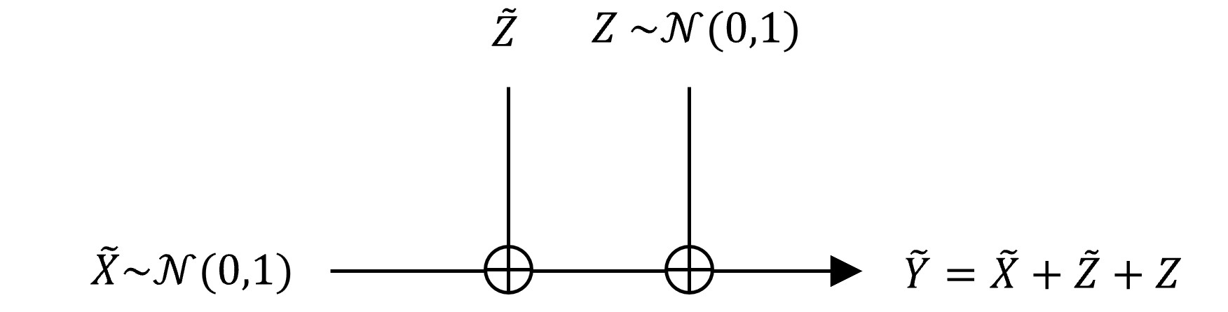
Consider the channel in Fig. 5, where $\tilde{X}$, $\tilde{Z}$ and $Z$ are independent, and $\int\vartheta^{2}f_{\tilde{Z}}(\vartheta)d\vartheta=P_{\!\tilde{Z}}$. Let us define

$$\hat{f} = f_{\tilde{X}}\ast f_{\tilde{Z}}\ast{\cal N}(0,1)$$ (60)

$$= f_{\tilde{Z}}+{\cal N}(0,2)$$ (61)

$$\check{f} = f_{\tilde{Z}}\ast{\cal N}(0,1)$$ (62)

where ${\cal N}(\mathfrak{u},\mathfrak{s})$ is a Gaussian density with statistical average $\mathfrak{u}$ and variance $\mathfrak{s}$. We have

$$I(\tilde{X};\tilde{Y})=\mathsf{H}^{\hat{f}}-\mathsf{H}^{\check{f}}$$ (63)

where $\mathsf{H}^{\hat{f}}$ and $\mathsf{H}^{\check{f}}$ are entropy values for densities $\hat{f}$ and $\check{f}$. It follows that

$$\min_{\hat{f},\check{f}}I(\tilde{X};\tilde{Y})\penalty 10000\ \penalty 10000\ \mbox{is achieved for} \!\!\!\!\!\!\!\!\!\!f_{\tilde{Z}}={\cal N}(0,P_{\!\tilde{Z}})$$ (64)

$$\max_{\hat{f},\check{f}}I(\tilde{X};\tilde{Y})\penalty 10000\ \penalty 10000\ \mbox{is achieved for} \!\!f_{\tilde{Z}}={\cal N}(\sqrt{P_{\!\tilde{Z}}},0).$$ (65)

A non-zero statistical mean entails the power $P_{\!\tilde{Z}}$ is intentionally wasted to avoid interference. $\blacksquare$

Theorem 8 establishes that the codebook densities corresponding to $U_{1}$, $V_{1}$, $U_{2}$, and $V_{2}$ are zero-mean. Consequently, all optimization problems can be formulated, without loss of optimality, in terms of zero-mean densities.

Theorem 8.

Code-books’ densities for (single letter) $U_{1}$, $V_{1}$, $U_{2}$, $V_{2}$ are zero mean for $\forall P_{1},\forall P_{2}$.

Proof.

For $\mu<1$, The codebook densities corresponding to the public messages $U_{1}$ and $U_{2}$ are zero-mean. The reason is that, instead of expending part of the power budgets $P_{U_{1}}$ and/or $P_{U_{2}}$ on non-zero mean values, the same power can be used to increase the variances of the corresponding codebooks. This, in turn, increases $R_{U_{1}}$ and/or $R_{U_{2}}$ while preserving the requirement that the public messages be decodable at both receivers. On the other hand, if the codebook densities corresponding to the private messages $V_{1}$ and/or $V_{2}$ have non-zero means, the power allocated to those means can instead be reassigned to the corresponding public messages. This strictly increases $R_{U_{1}}$ and/or $R_{U_{2}}$ while maintaining the decodability of both the public and private messages. ∎

It is of interest to derive explicit expressions and identify the conditions governing the formation of the various segments of the boundary. This task is challenging due to the large number of parameters involved and the intricate interplay among the corresponding conditions. Section 6 presents a method that significantly simplifies these derivations.

6 Covering the Boundary Through Incremental Power Reallocation

The capacity region in the single-letter case is covered by starting from the point that maximizes $R_{1}$ and proceeding counterclockwise along the lower boundary, corresponding to $\mu<1$. In a sequence of infinitesimal steps, $R_{2}$ is gradually increased in exchange for a decrease in $R_{1}$. Each step involves infinitesimal reallocations of power among the messages. The reallocated power amounts, denoted by $\delta P_{1}$ and $\delta P_{2}$, are chosen sufficiently small so that the coding strategy remains unchanged within the step; any change in strategy can occur only at the beginning of a subsequent step.

Consider an infinitesimal step from a starting point, denoted by superscript $s$, to an ending point, denoted by superscript $e$. The slope $\mathbf{\Upsilon}$ of such a step is defined as

$$\mathbf{\Upsilon}=\frac{\Delta\!R_{2}}{\Delta\!R_{1}}=\frac{R^{e}_{V_{2}}+R^{e}_{U_{2}}-R^{s}_{V_{2}}-R^{s}_{U_{2}}}{R^{s}_{V_{1}}+R^{s}_{U_{1}}-R^{e}_{V_{1}}-R^{e}_{U_{1}}}\triangleq\frac{\mathbf{N}}{\mathbf{D}}$$ (66)

where $(R^{s}_{U_{1}},R^{s}_{V_{1}})$ and $(R^{s}_{U_{2}},R^{s}_{V_{2}})$ denote the public and private rates of users 1 and 2, respectively, at the starting point. Likewise, $(R^{e}_{U_{1}},R^{e}_{V_{1}})$ and $(R^{e}_{U_{2}},R^{e}_{V_{2}})$ denote the corresponding public and private rates at the end point. Note that $\Delta R_{1}$ and $\Delta R_{2}$ are defined to be positive quantities. In particular, $\Delta R_{1}$ is defined as the rate $R_{1}$ at the starting point minus the rate $R_{1}$ at the end point. For a given value of $\mathbf{\Upsilon}$, the optimality of a boundary point is characterized by maximizing

$$\mathbf{\Gamma}=\sqrt{(\Delta R_{1})^{2}+(\Delta R_{2})^{2}}.$$ (67)

Theorem 9.

For $\mu<1$, consider a set of consecutive steps, in counterclockwise direction, along the boundary of the single letter capacity region based on 5 to 7. Corresponding values for $\mathbf{\Upsilon}$ in 66 will be monotonically decreasing, while $\mathbf{\Gamma}$ in 67 will be monotonically increasing.

Proof.

See Appendix B.1. ∎

Figure 6: $\mathbf{\Upsilon}$ and $\mathbf{\Gamma}$ as a function of $\omega$ (related to Theorem 10).

Next, consider a segment on the boundary from a starting point $\mathbb{S}$ to an end point $\mathbb{E}$ as depicted in Fig. 6. With some misuse of notation, superscripts are used to refer to points inside or on the boundary. Assume power reallocation vector for point $\mathbb{E}$ is equal to $({\delta}P^{\mathbb{E}}_{U_{1}},{\delta}P^{\mathbb{E}}_{V_{1}},{\delta}P^{\mathbb{E}}_{U_{2}},{\delta}P^{\mathbb{E}}_{V_{2}})$. Consider the line connecting points $\mathbb{S}$ and $\mathbb{E}$ with a time interpolation factor $\omega\in[0,1]$ where $\omega=0$ and $\omega=1$ correspond to points $\mathbb{S}$ and $\mathbb{E}$, respectively. Time interpolation achieves point $\mathbb{T}$ inside the capacity region, corresponding to an effective (interpolated) power reallocation vector $\omega({\delta}P^{\mathbb{E}}_{U_{1}},{\delta}^{\mathbb{E}}P_{V_{1}},{\delta}P^{\mathbb{E}}_{U_{2}},{\delta}P^{\mathbb{E}}_{V_{2}})$. Consider the power reallocation vector $\omega({\delta}P^{\mathbb{E}}_{U_{1}},{\delta}^{\mathbb{E}}P_{V_{1}},{\delta}P^{\mathbb{E}}_{U_{2}},{\delta}P^{\mathbb{E}}_{V_{2}})$ with optimum code-books’ densities, resulting in the point $\mathbb{B}$ on the boundary corresponding to $\mathbf{\Upsilon}^{\mathbb{B}}(\omega)$, $\mathbf{\Gamma}^{\mathbb{B}}(\omega)$. Relying on a simple time interpolation to achieve point $\mathbb{T}$ and optimum code-books’ densities to achieve points $\mathbb{E}$ and $\mathbb{B}$, we have

$$\mathbf{\Upsilon}^{\mathbb{B}} > \mathbf{\Upsilon}^{\mathbb{T}}\penalty 10000\ =\penalty 10000\ \mathbf{\Upsilon}^{\mathbb{E}}$$ (68)

$$\mathbf{\Gamma}^{\mathbb{B}} > \mathbf{\Gamma}^{\mathbb{T}}\penalty 10000\ =\penalty 10000\ \omega\mathbf{\Gamma}^{\mathbb{E}}.$$ (69)

Theorem 10.

Consider a segment of the boundary (limited to single-letter code-books) starting from a point $\mathbb{S}$ to a point $\mathbb{E}$. Power reallocation corresponding to $\omega({\delta}P^{\mathbb{E}}_{U_{1}},{\delta}^{\mathbb{E}}P_{V_{1}},{\delta}P^{\mathbb{E}}_{U_{2}},{\delta}P^{\mathbb{E}}_{V_{2}})$, in conjunction with independent and identical Gaussian code-books, solves the following constrained optimization problems:

Maximize $$\penalty 10000\ \mathbf{\Gamma}(\omega)\penalty 10000\ \penalty 10000\ \penalty 10000\ \penalty 10000\ \penalty 10000\ \mbox{subject to}\penalty 10000\ \penalty 10000\ \penalty 10000\ \penalty 10000\ \mathbf{\Upsilon}(\omega)\,\geq\hat{\mathbf{\Upsilon}}$$ (70)

Maximize $$\Delta\!R_{2}(\omega)\penalty 10000\ \penalty 10000\ \penalty 10000\ \mbox{subject to}\penalty 10000\ \penalty 10000\ \penalty 10000\ \Delta\!R_{1}(\omega)\leq\hat{\Delta}\!R_{1}$$ (71)

Minimize $$\Delta\!R_{1}(\omega)\penalty 10000\ \penalty 10000\ \penalty 10000\ \mbox{subject to}\penalty 10000\ \penalty 10000\ \penalty 10000\ \Delta\!R_{2}(\omega)\geq\hat{\Delta}\!R_{2}$$ (72)

Maximize $$\penalty 10000\ R_{2}(\omega)\penalty 10000\ \penalty 10000\ \penalty 10000\ \penalty 10000\ \mbox{subject to}\penalty 10000\ \penalty 10000\ \penalty 10000\ \penalty 10000\ R_{1}(\omega)\geq\hat{R}_{1}$$ (73)

Maximize $$\penalty 10000\ R_{1}(\omega)\penalty 10000\ \penalty 10000\ \penalty 10000\ \penalty 10000\ \mbox{subject to}\penalty 10000\ \penalty 10000\ \penalty 10000\ \penalty 10000\ R_{2}(\omega)\geq\hat{R}_{2}$$ (74)

for given $\hat{\mathbf{\Upsilon}}$, $\hat{\Delta}\!R_{1}$, $\hat{\Delta}\!R_{2}$, $\hat{R}_{1}$ and $\hat{R}_{2}$.

Proof.

See Appendix B.2. ∎

Next, Theorem 11, together with the fact that a zero-mean Gaussian density is completely characterized by its second moment, establishes that each boundary point is achieved by a unique single-letter Gaussian codebook for every $P_{1}$, every $P_{2}$, and every $\mu<1$.

Theorem 11.

Consider two distinct power allocation (over messages) vectors achieving the same value for $R_{1}+\mu R_{2}$. This is possible only for $\mu=1$.

Proof.

See Appendix B.3. ∎

Next, the condition for a power reallocation vector to be boundary achieving is discussed. Let us consider a step along the boundary which is small enough such that the coding strategy remains the same within the step. Let us assume $(\hat{\Delta}\!P_{1},\hat{\Delta}\!P_{2})$ is the power reallocation vector corresponding to an end point beyond which a change in strategy is needed, and consider

$$(\Delta\!P_{1},\Delta\!P_{2}):\Delta\!P_{1}\leq\hat{\Delta}\!P_{1}\penalty 10000\ \penalty 10000\ \mbox{and}\penalty 10000\ \penalty 10000\ \Delta\!P_{2}\leq\hat{\Delta}\!P_{2}.$$ (75)

Let us define $\upsilon\leq\mu^{s}$, where $\mu^{s}$ is the value of $\mu$ at the starting point, and the set $\bar{\mathsf{S}}_{\upsilon}$ as

$$\bar{\mathsf{S}}_{\upsilon}=\left\{f_{U_{1}},f_{V_{1}},f_{U_{2}},f_{V_{2}}\!:\!\penalty 10000\ \mbox{outgoing slope at the starting point is}\penalty 10000\ \upsilon\triangleq\min_{(\delta P_{1},\delta P_{2})\in[0,\Delta\!P_{1}]\times[0,\Delta\!P_{2}]}\mathbf{\Upsilon}\right\}.$$ (76)

Set $\bar{\mathsf{S}}_{\upsilon}$ is defined over all possible code-books’ densities, including Gaussian. Each member of 76 corresponds to a power reallocation vector $(\delta P_{1},\delta P_{2})\in[0,\Delta\!P_{1}]\times[0,\Delta\!P_{2}]$. This correspondence is potentially many-to-one since multiple choices for densities $(f_{U_{1}},f_{V_{1}},f_{U_{2}},f_{V_{2}})$, with the same $(\delta P_{1},\delta P_{2})$, may achieve the same $\mathbf{\Upsilon}=\upsilon$. Given $\mathbf{\Upsilon}=\upsilon$, the size of the set $\bar{\mathsf{S}}_{\upsilon}$ is reduced by limiting it to choice(s) which maximize $\mathbf{\Gamma}$. Maximum value of $\mathbf{\Gamma}$ over the set $\bar{\mathsf{S}}_{\upsilon}$ is denoted as $\varkappa_{\upsilon}$. Let us consider a second set $\bar{\bar{\mathsf{S}}}_{\upsilon}$ where

$$\bar{\bar{\mathsf{S}}}_{\upsilon}\subseteq\bar{\mathsf{S}}_{\upsilon}:\penalty 10000\ \mathbf{\Gamma}=\varkappa_{\upsilon}.$$ (77)

The set $\bar{\bar{\mathsf{S}}}_{\upsilon}$ includes a point on the boundary with

$$\mathbf{\Upsilon}=\upsilon\penalty 10000\ \penalty 10000\ \mbox{and}\penalty 10000\ \penalty 10000\ \mathbf{\Gamma}=\varkappa_{\upsilon}\triangleq\max_{\mathbf{\Upsilon}=\upsilon}\mathbf{\Gamma}.$$ (78)

We are interested in establishing that the size of $\bar{\bar{\mathsf{S}}}_{\upsilon}$ can be reduced, by increasing $\upsilon$, such that the shrunken set includes a single element, say $\zeta$. Since $\bar{\bar{\mathsf{S}}}_{\upsilon}$ always includes a point on the boundary, it follows that $\zeta$ falls on the boundary. In addition, we need to show that the rest of the boundary can be covered starting from $\zeta$. Theorem 12 addresses these requirements.

Theorem 12.

Cardinality of the set $\bar{\bar{\mathsf{S}}}_{\upsilon}$ can be reduced, by increasing $\upsilon<\mu^{s}$, in a recursive manner, such that the final set is associated with a single $(\delta P_{1},\delta P_{2})$.

Proof.

See Appendix B.4. ∎

Referring to Theorem 12, using $(\breve{\delta}P_{1},\breve{\delta}P_{2})$ instead of $(\delta^{m}P_{1},\delta^{m}P_{2})$, $m=1,\ldots,M$ (see expression 223) is accompanied by a movement in clockwise direction, i.e., reaching from $(\upsilon,\gamma)$ to $(\breve{\upsilon},\breve{\gamma})$, where

$$(\upsilon,\varkappa_{\upsilon})\leadsto(\breve{\upsilon},\varkappa_{\breve{\upsilon}}):\penalty 10000\ \penalty 10000\ \breve{\upsilon}>\upsilon\penalty 10000\ \penalty 10000\ \mbox{and}\penalty 10000\ \penalty 10000\ \varkappa_{\breve{\upsilon}}<\varkappa_{\upsilon}.$$ (79)

Such a movement can continue in a recursive manner until the step size is small enough to include a single power reallocation vector, i.e.,

$$\exists i\in[1,\ldots,M]:\penalty 10000\ (\breve{\delta}P_{1},\breve{\delta}P_{2})=(\delta^{i}P_{1},\delta^{i}P_{2})$$ (80)

with the resulting $(\breve{\delta}P_{1},\breve{\delta}P_{2})$ achieving to a unique point on the boundary. Theorem 12 entails, relying on Pareto minimal power reallocation, the past history in moving counterclockwise along the boundary is captured solely by the starting point in each step.

Remark 3: The optimum Pareto minimal power reallocation vector is not unique. However, the corresponding set has a nested structure, and relying on any member of the set will be associated with a unique set of Gaussian code-books. Different members of the set of Pareto minimal power reallocation pairs correspond to different step sizes. This property allows covering the boundary in a continuous manner. To clarify this point, let us consider two nested Pareto minimal power reallocation vectors $(\dot{\delta}P_{1},\dot{\delta}P_{2})$ and $(\ddot{\delta}P_{1},\ddot{\delta}P_{2})$, where

$$\dot{\delta}P_{1}\leq\ddot{\delta}P_{1}\penalty 10000\ \penalty 10000\ \mbox{and}\penalty 10000\ \penalty 10000\ \dot{\delta}P_{2}\leq\ddot{\delta}P_{2}.$$ (81)

These power reallocation vectors, in conjunction with Gaussian code-books, achieve two successive points on the boundary, namely

$$(\mathbf{\Upsilon}_{\!1},\mathbf{\Gamma}_{\!1})=(\dot{\upsilon},\varkappa_{\dot{\upsilon}})\penalty 10000\ \penalty 10000\ \mbox{and}\penalty 10000\ \penalty 10000\ (\mathbf{\Upsilon}_{\!2},\mathbf{\Gamma}_{\!2})=(\ddot{\upsilon},\varkappa_{\ddot{\upsilon}})$$ (82)

satisfying $\ddot{\upsilon}\leq\dot{\upsilon}\penalty 10000\ \penalty 10000\ \mbox{and}\penalty 10000\ \penalty 10000\ \varkappa_{\ddot{\upsilon}}\geq\varkappa_{\dot{\upsilon}}.$ $\blacksquare$

7 Converse Results

Consider a phase where both users are active, together with a given power allocation over messages, and given codebooks’ densities. Without loss of generality, let us consider the case that $U_{2}$ is first decoded at $Y_{1}$, followed by successive decoding of $U_{1}$ and $V_{1}$, we have

$$\ \mathfrak{r}_{\mathtt{u}_{1}}+\mathfrak{r}_{\mathtt{u}_{2}} = I(\mathtt{u}_{1},\mathtt{u}_{2};\mathtt{y}_{1})=\overbrace{I(\mathtt{u}_{2};\mathtt{y}_{1})+I(\mathtt{u}_{1};\mathtt{y}_{1}|\mathtt{u}_{2})}^{\mbox{\scriptsize Successive Decoding}}=\overbrace{I(\mathtt{u}_{1},\mathtt{u}_{2};\mathtt{y}_{2})}^{\mbox{\scriptsize Joint Decoding}}$$ (83)

$$\mathfrak{r}_{\mathtt{u}_{2}} = I(\mathtt{u}_{2};\mathtt{y}_{1})$$ (84)

$$\mathfrak{r}_{\mathtt{u}_{1}} = I(\mathtt{u}_{1};\mathtt{y}_{1}|\mathtt{u}_{2})$$ (85)

$$\mathfrak{r}_{\mathtt{v}_{1}} = I(\mathtt{v}_{1};\mathtt{y}_{1}|\mathtt{u}_{1},\mathtt{u}_{2})$$ (86)

$$\mathfrak{r}_{\mathtt{v}_{2}} = I(\mathtt{v}_{2};\mathtt{y}_{2}|\mathtt{u}_{1},\mathtt{u}_{2}).$$ (87)

Theorem 13.

If probability of error in recovering $\mathtt{u}_{1},\mathtt{u}_{2},\mathtt{v}_{1}$ at $\mathtt{y}_{1}$ and $\mathtt{u}_{1},\mathtt{u}_{2},\mathtt{v}_{2}$ at $\mathtt{y}_{2}$ tend to zero as $\mathtt{t}\rightarrow\infty$, then the rate vector $(\mathfrak{R}_{1}=\mathfrak{r}_{\mathtt{u}_{1}}+\mathfrak{r}_{\mathtt{v}_{1}},\mathfrak{R}_{2}=\mathfrak{r}_{\mathtt{u}_{2}}+\mathfrak{r}_{\mathtt{v}_{2}})$ should fall within the optimum region with independent and identically distributed single letter Gaussian code-books.

Proof.

Let us consider the channel models in Fig. 4 in conjunction with vectors $\mathtt{u}_{1},\mathtt{v}_{1},\mathtt{u}_{2},\mathtt{v}_{2}$. Let us assume the set of rates $(\check{\mathfrak{r}}_{\mathtt{u}_{1}},\check{\mathfrak{r}}_{\mathtt{u}_{2}},\check{\mathfrak{r}}_{\mathtt{v}_{1}},\check{\mathfrak{r}}_{\mathtt{v}_{2}})$. For the decoding strategies in 83 to 87, let us consider the following cases

$$\mbox{Case 1:\penalty 10000\ \penalty 10000\ \penalty 10000\ }\check{\mathfrak{r}}_{\mathtt{u}_{1}}\geq\mathfrak{r}_{\mathtt{u}_{1}},\,\check{\mathfrak{r}}_{\mathtt{u}_{2}}>\mathfrak{r}_{\mathtt{u}_{2}},\,\check{\mathfrak{r}}_{\mathtt{v}_{1}}\geq\mathfrak{r}_{\mathtt{v}_{1}},\,\check{\mathfrak{r}}_{\mathtt{v}_{2}}\geq\mathfrak{r}_{\mathtt{v}_{2}} \Longrightarrow P^{\,e}_{\mathtt{u}_{1}}>0,\,P^{\,e}_{\mathtt{u}_{2}}>0,\,P^{\,e}_{\mathtt{v}_{1}}>0,\,P^{\,e}_{\mathtt{v}_{2}}>0$$ (88)

$$\mbox{Case 2:\penalty 10000\ \penalty 10000\ \penalty 10000\ }\check{\mathfrak{r}}_{\mathtt{u}_{1}}>\mathfrak{r}_{\mathtt{u}_{1}},\,\check{\mathfrak{r}}_{\mathtt{u}_{2}}\geq\mathfrak{r}_{\mathtt{u}_{2}},\,\check{\mathfrak{r}}_{\mathtt{v}_{1}}\geq\mathfrak{r}_{\mathtt{v}_{1}},\,\check{\mathfrak{r}}_{\mathtt{v}_{2}}\geq\mathfrak{r}_{\mathtt{v}_{2}} \Longrightarrow P^{\,e}_{\mathtt{u}_{1}}>\,0,P^{\,e}_{\mathtt{u}_{2}}>\,0,P^{\,e}_{\mathtt{v}_{1}}>\,0,P^{\,e}_{\mathtt{v}_{2}}>\,0$$ (89)

$$\mbox{Case 3:\penalty 10000\ \penalty 10000\ \penalty 10000\ }\check{\mathfrak{r}}_{\mathtt{u}_{1}}\geq\mathfrak{r}_{\mathtt{u}_{1}},\,\check{\mathfrak{r}}_{\mathtt{u}_{2}}\geq\mathfrak{r}_{\mathtt{u}_{2}},\,\check{\mathfrak{r}}_{\mathtt{v}_{1}}>\mathfrak{r}_{\mathtt{v}_{1}},\,\check{\mathfrak{r}}_{\mathtt{v}_{2}}\geq\mathfrak{r}_{\mathtt{v}_{2}} \Longrightarrow P^{\,e}_{\mathtt{u}_{1}}\geq 0,\,P^{\,e}_{\mathtt{u}_{2}}\geq 0,\,P^{\,e}_{\mathtt{v}_{1}}>0,\,P^{\,e}_{\mathtt{v}_{2}}\geq 0$$ (90)

$$\mbox{Case 4:\penalty 10000\ \penalty 10000\ \penalty 10000\ }\check{\mathfrak{r}}_{\mathtt{u}_{1}}\geq\mathfrak{r}_{\mathtt{u}_{1}},\,\check{\mathfrak{r}}_{\mathtt{u}_{2}}\geq\mathfrak{r}_{\mathtt{u}_{2}},\,\check{\mathfrak{r}}_{\mathtt{v}_{1}}\geq\mathfrak{r}_{\mathtt{v}_{1}},\,\check{\mathfrak{r}}_{\mathtt{v}_{2}}>\mathfrak{r}_{\mathtt{v}_{2}} \Longrightarrow P^{\,e}_{\mathtt{u}_{1}}\geq 0,\,P^{\,e}_{\mathtt{u}_{2}}\geq 0,\,P^{\,e}_{\mathtt{v}_{1}}\geq 0,\,P^{\,e}_{\mathtt{v}_{2}}>0.$$ (91)

Expressions 88 and 89 reflect the fact that in case 1 and case 2, public messages $(U_{1},U_{2})$ can be recovered/removed neither at $Y_{1}$ nor at $Y_{2}$. This causes error propagation to the recovery of $V_{1}$ at $Y_{1}$ and $V_{2}$ at $Y_{2}$. If $(U_{1},U_{2})$ can be recovered/removed at both receivers, then cases 3 and 4 can be expressed as

$$\check{\mathfrak{r}}_{\mathtt{u}_{1}}=\mathfrak{r}_{\mathtt{u}_{1}},\,\,\check{\mathfrak{r}}_{\mathtt{u}_{2}}=\mathfrak{r}_{\mathtt{u}_{2}},\,\,\check{\mathfrak{r}}_{\mathtt{v}_{1}}>\mathfrak{r}_{\mathtt{v}_{1}},\,\,\check{\mathfrak{r}}_{\mathtt{v}_{2}}\geq\mathfrak{r}_{\mathtt{v}_{2}} \Longrightarrow P^{\,e}_{\mathtt{u}_{1}}=0,\,P^{\,e}_{\mathtt{u}_{2}}=0,\,P^{\,e}_{\mathtt{v}_{1}}>0,\,P^{\,e}_{\mathtt{v}_{2}}\geq 0.$$ (92)

$$\check{\mathfrak{r}}_{\mathtt{u}_{1}}=\mathfrak{r}_{\mathtt{u}_{1}},\,\,\check{\mathfrak{r}}_{\mathtt{u}_{2}}=\mathfrak{r}_{\mathtt{u}_{2}},\,\,\check{\mathfrak{r}}_{\mathtt{v}_{1}}\geq\mathfrak{r}_{\mathtt{v}_{1}},\,\,\check{\mathfrak{r}}_{\mathtt{v}_{2}}>\mathfrak{r}_{\mathtt{v}_{2}} \Longrightarrow P^{\,e}_{\mathtt{u}_{1}}=0,\,P^{\,e}_{\mathtt{u}_{2}}=0,\,P^{\,e}_{\mathtt{v}_{1}}\geq 0,\,P^{\,e}_{\mathtt{v}_{2}}>0.$$ (93)

Above arguments establish that if any rate in 83 to 87 exceeds its corresponding mutual information bound, then, for the decoding strategy given in 83 to 87, it would be impossible to achieve

$$P^{\,e}_{\mathtt{u}_{1}}=0,\penalty 10000\ \penalty 10000\ P^{\,e}_{\mathtt{v}_{1}}=0,\penalty 10000\ \penalty 10000\ P^{\,e}_{\mathtt{u}_{2}}=0,\penalty 10000\ \penalty 10000\ P^{\,e}_{\mathtt{v}_{2}}=0.$$ (94)

The final step in the proof follows noting that, for any given $\mu$, the region based on 83 to 87 maximizes

$$\mathfrak{r}_{1}+\mu\mathfrak{r}_{2}=\mathfrak{r}_{\mathtt{u}_{1}}+\mathfrak{r}_{\mathtt{v}_{1}}+\mu(\mathfrak{r}_{\mathtt{u}_{2}}+\mathfrak{r}_{\mathtt{v}_{2}})$$ (95)

by using independent and identically distributed single letter Gaussian code-books, while optimizing the corresponding weighted sum-rate over bandwidth allocation (between phases) and power allocation (between messages/phases). This means in such an optimally enlarged region, if any of the rates exceed the mutual information terms on the right hand sides of 83 to 87, the error probability for $(\mathtt{u}_{1},\mathtt{v}_{1})$ and/or $(\mathtt{u}_{2},\mathtt{v}_{2})$ will be bounded away from zero. ∎

Next, it will be shown that the Han-Kobayashi (HK) achievable rate region, after potentially restricting its feasible set through the imposition of additional but consistent constraints, attains the boundary of the capacity region.

8 Optimality of the HK Region with Gaussian Code-books

Let us consider the Expanded Han-Kobayashi constraints can be expressed as [5],

Maximize: $$R_{1}+\mu R_{2}=R_{U_{1}}+R_{V_{1}}+\mu R_{U_{2}}+\mu R_{V_{2}}\penalty 10000\ \mbox{where}$$ (96)

$$R_{U_{1}} \penalty 10000\ \penalty 10000\ {\leq}\penalty 10000\ \penalty 10000\ I(U_{1};Y_{1}|U_{2},V_{1})$$ (97)

$$R_{U_{1}} \penalty 10000\ \penalty 10000\ {\leq}\penalty 10000\ \penalty 10000\ I(U_{1};Y_{2}|U_{2},V_{2})$$ (98)

$$R_{U_{2}} \penalty 10000\ \penalty 10000\ {\leq}\penalty 10000\ \penalty 10000\ I(U_{2};Y_{1}|U_{1},V_{1})$$ (99)

$$R_{U_{2}} \penalty 10000\ \penalty 10000\ {\leq}\penalty 10000\ \penalty 10000\ I(U_{2};Y_{2}|U_{1},V_{2})$$ (100)

$$R_{V_{1}} \penalty 10000\ \penalty 10000\ {\leq}\penalty 10000\ \penalty 10000\ I(V_{1};Y_{1}|U_{1},U_{2})$$ (101)

$$R_{V_{2}} \penalty 10000\ \penalty 10000\ {\leq}\penalty 10000\ \penalty 10000\ I(V_{2};Y_{2}|U_{1},U_{2})$$ (102)

$$R_{U_{1}}+R_{U_{2}} \penalty 10000\ \penalty 10000\ {\leq}\penalty 10000\ \penalty 10000\ I(U_{1},U_{2};Y_{1}|V_{1})$$ (103)

$$R_{U_{1}}+R_{U_{2}} \penalty 10000\ \penalty 10000\ {\leq}\penalty 10000\ \penalty 10000\ I(U_{1},U_{2};Y_{2}|V_{2})$$ (104)

$$R_{U_{1}}+R_{V_{1}} \penalty 10000\ \penalty 10000\ {\leq}\penalty 10000\ \penalty 10000\ I(U_{1},V_{1};Y_{1}|U_{2})=I(U_{1};Y_{1}|U_{2})+I(V_{1};Y_{1}|U_{1},U_{2})$$ (105)

$$R_{U_{2}}+R_{V_{2}} \penalty 10000\ \penalty 10000\ {\leq}\penalty 10000\ \penalty 10000\ I(U_{2},V_{2};Y_{2}|U_{1})=I(U_{2};Y_{2}|U_{1})+I(V_{2};Y_{2}|U_{1},U_{2})$$ (106)

$$R_{U_{2}}+R_{V_{1}} \penalty 10000\ \penalty 10000\ {\leq}\penalty 10000\ \penalty 10000\ I(U_{2},V_{1};Y_{1}|U_{1})=I(U_{2};Y_{1}|U_{1})+I(V_{1};Y_{1}|U_{1},U_{2})$$ (107)

$$R_{U_{1}}+R_{V_{2}} \penalty 10000\ \penalty 10000\ {\leq}\penalty 10000\ \penalty 10000\ I(U_{1},V_{2};Y_{2}|U_{2})=I(U_{1};Y_{2}|U_{2})+I(V_{2};Y_{2}|U_{1},U_{2})$$ (108)

$$R_{U_{1}}+R_{U_{2}}+R_{V_{1}} \penalty 10000\ \penalty 10000\ {\leq}\penalty 10000\ \penalty 10000\ I(U_{1},U_{2},V_{1};Y_{1})=I(U_{1},U_{2};Y_{1})+I(V_{1};Y_{1}|U_{1},U_{2})$$ (109)

$$R_{U_{1}}+R_{U_{2}}+R_{V_{2}} \penalty 10000\ \penalty 10000\ {\leq}\penalty 10000\ \penalty 10000\ I(U_{1},U_{2},V_{2};Y_{2})=I(U_{1},U_{2};Y_{2})+I(V_{2};Y_{2}|U_{1},U_{2})$$ (110)

$$E(X_{1}^{2}) \penalty 10000\ \penalty 10000\ =\penalty 10000\ \penalty 10000\ P_{1}$$ (111)

$$E(X_{2}^{2}) \penalty 10000\ \penalty 10000\ =\penalty 10000\ \penalty 10000\ P_{2}.$$ (112)

Let us consider 96 to 110 in conjunction with independent and identically distributed (single-letter) Gaussian code-books for $U_{1}$, $U_{2}$, $V_{1}$, $V_{2}$. For Gaussian code-books, the degradedness properties established in Theorem 3 are valid. Since the above formulation results in an achievable weighted sum-rate, any set of restrictive assumptions, if consistent with 96 to 112, results in an achievable (potentially inferior) solution. Let us restrict $U_{1}$, $U_{2}$, $V_{1}$, $V_{2}$ to be independent, $X_{1}=U_{1}+V_{1}$, $X_{2}=U_{2}+V_{2}$. We have $E(X_{1}^{2})=E(U_{1}^{2})+E(V_{1}^{2})$ and $E(X_{2}^{2})=E(U_{2}^{2})+E(V_{2}^{2})$. For given power allocation and encoding/decoding strategies (determining the values of mutual information terms on right hand sides of 97 to 110), optimization problem in 96 to 110 will be a linear programming problem with four variables, i.e., $R_{U_{1}}$, $R_{U_{2}}$, $R_{V_{1}}$, $R_{V_{2}}$. This means, in the optimum solution, at least 4 constraints among 97 to 110 will be satisfied with equality, resulting in zero value for the corresponding slack variables

Let us further restrict the HK region by imposing

$$R_{V_{1}}=I(V_{1};Y_{1}|U_{1},U_{2}),\penalty 10000\ \penalty 10000\ \penalty 10000\ R_{V_{2}}=I(V_{2};Y_{2}|U_{1},U_{2}),\penalty 10000\ \penalty 10000\ \penalty 10000\ R_{U_{1}}+R_{U_{2}}=I(U_{1},U_{2};Y_{1})=I(U_{1},U_{2};Y_{2}).$$ (113)

For such a restricted region, we have

Maximize: $$R_{1}+\mu R_{2}=R_{U_{1}}+R_{V_{1}}+\mu R_{U_{2}}+\mu R_{V_{2}}\penalty 10000\ \mbox{where}$$ (114)

$$R_{U_{1}} \penalty 10000\ \penalty 10000\ {\leq}\penalty 10000\ \penalty 10000\ I(U_{1};Y_{1}|U_{2})\penalty 10000\ \stackrel{{\scriptstyle\text{(a)}}}{{\leq}}\penalty 10000\ I(U_{1};Y_{1}|U_{2},V_{1})$$ (115)

$$R_{U_{1}} \penalty 10000\ \penalty 10000\ {\leq}\penalty 10000\ \penalty 10000\ I(U_{1};Y_{2}|U_{2})\penalty 10000\ \stackrel{{\scriptstyle\text{(b)}}}{{\leq}}\penalty 10000\ I(U_{1};Y_{2}|U_{2},V_{2})$$ (116)

$$R_{U_{2}} \penalty 10000\ \penalty 10000\ {\leq}\penalty 10000\ \penalty 10000\ I(U_{2};Y_{1}|U_{1})\penalty 10000\ \stackrel{{\scriptstyle\text{(c)}}}{{\leq}}\penalty 10000\ I(U_{2};Y_{1}|U_{1},V_{1})$$ (117)

$$R_{U_{2}} \penalty 10000\ \penalty 10000\ {\leq}\penalty 10000\ \penalty 10000\ I(U_{2};Y_{2}|U_{1})\penalty 10000\ \stackrel{{\scriptstyle\text{(d)}}}{{\leq}}\penalty 10000\ I(U_{2};Y_{2}|U_{1},V_{2})$$ (118)

$$R_{U_{1}}+R_{U_{2}} \penalty 10000\ \penalty 10000\ \stackrel{{\scriptstyle\text{(e)}}}{{=}}\penalty 10000\ I(U_{1},U_{2};Y_{1})$$ (119)

$$R_{U_{1}}+R_{U_{2}} \penalty 10000\ \penalty 10000\ \stackrel{{\scriptstyle\text{(f)}}}{{=}}\penalty 10000\ \penalty 10000\ I(U_{1},U_{2};Y_{2})$$ (120)

$$R_{V_{1}} \penalty 10000\ \penalty 10000\ {=}\penalty 10000\ \penalty 10000\ I(V_{1};Y_{1}|U_{1},U_{2})$$ (121)

$$R_{V_{2}} \penalty 10000\ \penalty 10000\ {=}\penalty 10000\ \penalty 10000\ I(V_{2};Y_{2}|U_{1},U_{2})$$ (122)

$$R_{U_{1}} \penalty 10000\ \penalty 10000\ \stackrel{{\scriptstyle\text{(a)}}}{{\leq}}\penalty 10000\ \penalty 10000\ I(U_{1};Y_{1}|U_{2},V_{1})$$ (123)

$$R_{U_{1}} \penalty 10000\ \penalty 10000\ \stackrel{{\scriptstyle\text{(b)}}}{{\leq}}\penalty 10000\ \penalty 10000\ I(U_{1};Y_{2}|U_{2},V_{2})$$ (124)

$$R_{U_{2}} \penalty 10000\ \penalty 10000\ \stackrel{{\scriptstyle\text{(c)}}}{{\leq}}\penalty 10000\ \penalty 10000\ I(U_{2};Y_{1}|U_{1},V_{1})$$ (125)

$$R_{U_{2}} \penalty 10000\ \penalty 10000\ \stackrel{{\scriptstyle\text{(d)}}}{{\leq}}\penalty 10000\ \penalty 10000\ I(U_{2};Y_{2}|U_{1},V_{2})$$ (126)

$$R_{U_{1}}+R_{U_{2}} \penalty 10000\ \penalty 10000\ {\leq}\penalty 10000\ \penalty 10000\ I(U_{1},U_{2};Y_{1}|V_{1})\penalty 10000\ \stackrel{{\scriptstyle\text{(e)}}}{{\leq}}\penalty 10000\ I(U_{1},U_{2};Y_{1})$$ (127)

$$R_{U_{1}}+R_{U_{2}} \penalty 10000\ \penalty 10000\ {\leq}\penalty 10000\ \penalty 10000\ I(U_{1},U_{2};Y_{2}|V_{2})\penalty 10000\ \stackrel{{\scriptstyle\text{(f)}}}{{\leq}}\penalty 10000\ I(U_{1},U_{2};Y_{2})$$ (128)

$$E(X_{1}^{2}) \penalty 10000\ \penalty 10000\ =\penalty 10000\ \penalty 10000\ P_{1}$$ (129)

$$E(X_{2}^{2}) \penalty 10000\ \penalty 10000\ =\penalty 10000\ \penalty 10000\ P_{2}.$$ (130)

Noting relationships specified by (a),(b),(c),(d),(e) and (f) in 114 to 128, it follows that 123 to 128 are redundant. Upon removing redundant constraints from 114 to 130, we obtain

Maximize: $$R_{1}+\mu R_{2}\penalty 10000\ \penalty 10000\ \penalty 10000\ \mbox{where}$$ (131)

$$R_{U_{1}} \penalty 10000\ \penalty 10000\ {\leq}\penalty 10000\ \penalty 10000\ I(U_{1};Y_{1}|U_{2})$$ (132)

$$R_{U_{1}} \penalty 10000\ \penalty 10000\ {\leq}\penalty 10000\ \penalty 10000\ I(U_{1};Y_{2}|U_{2})$$ (133)

$$R_{U_{2}} \penalty 10000\ \penalty 10000\ {\leq}\penalty 10000\ \penalty 10000\ I(U_{2};Y_{1}|U_{1})$$ (134)

$$R_{U_{2}} \penalty 10000\ \penalty 10000\ {\leq}\penalty 10000\ \penalty 10000\ I(U_{2};Y_{2}|U_{1})$$ (135)

$$R_{U_{1}}+R_{U_{2}} \penalty 10000\ \penalty 10000\ {=}\penalty 10000\ \penalty 10000\ I(U_{1},U_{2};Y_{1})$$ (136)

$$R_{U_{1}}+R_{U_{2}} \penalty 10000\ \penalty 10000\ {=}\penalty 10000\ \penalty 10000\ I(U_{1},U_{2};Y_{2})$$ (137)

$$R_{V_{1}} \penalty 10000\ \penalty 10000\ {=}\penalty 10000\ \penalty 10000\ I(V_{1};Y_{1}|U_{1},U_{2})$$ (138)

$$R_{V_{2}} \penalty 10000\ \penalty 10000\ {=}\penalty 10000\ \penalty 10000\ I(V_{2};Y_{2}|U_{1},U_{2})$$ (139)

$$E(X_{1}^{2}) \penalty 10000\ \penalty 10000\ =\penalty 10000\ \penalty 10000\ P_{1}$$ (140)

$$E(X_{2}^{2}) \penalty 10000\ \penalty 10000\ =\penalty 10000\ \penalty 10000\ P_{2}.$$ (141)

Let us consider the following problem:

Maximize: $$R_{1}+\mu R_{2}\penalty 10000\ \penalty 10000\ \penalty 10000\ \mbox{where}$$ (142)

$$R_{U_{1}} \penalty 10000\ \penalty 10000\ {=}\penalty 10000\ \penalty 10000\ I(U_{1};Y_{2}|U_{2})\stackrel{{\scriptstyle\text{(g)}}}{{\leq}}I(U_{1};Y_{1}|U_{2})$$ (143)

$$R_{U_{2}} \penalty 10000\ \penalty 10000\ {=}\penalty 10000\ \penalty 10000\ I(U_{2};Y_{1})\leq I(U_{2};Y_{1}|U_{1})\stackrel{{\scriptstyle\text{(h)}}}{{\leq}}\penalty 10000\ I(U_{2};Y_{2}|U_{1})$$ (144)

$$R_{U_{1}}+R_{U_{2}} \penalty 10000\ \penalty 10000\ {=}\penalty 10000\ \penalty 10000\ I(U_{1},U_{2};Y_{1})$$ (145)

$$R_{U_{1}}+R_{U_{2}} \penalty 10000\ \penalty 10000\ {=}\penalty 10000\ \penalty 10000\ I(U_{1},U_{2};Y_{2})$$ (146)

$$R_{V_{1}} \penalty 10000\ \penalty 10000\ {=}\penalty 10000\ \penalty 10000\ I(V_{1};Y_{1}|U_{1},U_{2})$$ (147)

$$R_{V_{2}} \penalty 10000\ \penalty 10000\ {=}\penalty 10000\ \penalty 10000\ I(V_{2};Y_{2}|U_{1},U_{2})$$ (148)

$$E(X_{1}^{2}) \penalty 10000\ \penalty 10000\ =\penalty 10000\ \penalty 10000\ P_{1}$$ (149)

$$E(X_{2}^{2}) \penalty 10000\ \penalty 10000\ =\penalty 10000\ \penalty 10000\ P_{2}$$ (150)

where $(g)$ in 142 and $(h)$ in 144 are from Theorem 3. The solution to 142 to 150 is potentially inferior to the solution of the problem in 131 to 141, since the feasible region is shrunk by enforcing equality/inequality conditions in 143 and 144. Simplifying 142 to 150 results in

Maximize: $$R_{1}+\mu R_{2}\penalty 10000\ \penalty 10000\ \penalty 10000\ \mbox{where}$$ (151)

$$R_{U_{1}} \penalty 10000\ \penalty 10000\ {=}\penalty 10000\ \penalty 10000\ I(U_{1};Y_{1}|U_{2})$$ (152)

$$R_{U_{2}} \penalty 10000\ \penalty 10000\ {=}\penalty 10000\ \penalty 10000\ I(U_{2};Y_{1})$$ (153)

$$R_{U_{1}}+R_{U_{2}} \penalty 10000\ \penalty 10000\ {=}\penalty 10000\ \penalty 10000\ I(U_{1},U_{2};Y_{2})\penalty 10000\ =\penalty 10000\ I(U_{1},U_{2};Y_{1})$$ (154)

$$R_{V_{1}} \penalty 10000\ \penalty 10000\ {=}\penalty 10000\ \penalty 10000\ I(V_{1};Y_{1}|U_{1},U_{2})$$ (155)

$$R_{V_{2}} \penalty 10000\ \penalty 10000\ {=}\penalty 10000\ \penalty 10000\ I(V_{2};Y_{2}|U_{1},U_{2})$$ (156)

$$E(X_{1}^{2}) \penalty 10000\ \penalty 10000\ =\penalty 10000\ \penalty 10000\ P_{1}$$ (157)

$$E(X_{2}^{2}) \penalty 10000\ \penalty 10000\ =\penalty 10000\ \penalty 10000\ P_{2}.$$ (158)

Solution to 151 to 158 results: (1) an achievable region potentially inferior to the HK region due to shrinking of the corresponding feasible region, and (2) the solution coincides with optimum boundary established in Section 5 for $\mu<1$. Similar arguments can be applied to $\mu>1$. This entails Han-Kobayashi region with independent and identically distributed (single-letter) Gaussian code-books for $U_{1}$, $U_{2}$, $V_{1}$, $V_{2}$ is optimum.

Appendix

In the following, to simplify expressions, entropy values are computed in base “e".

Appendix A Optimality of Gaussian Code-books

A.1 Preliminaries

LICQ should be verified in relation to active constraints in 36 to 40. For simplicity, without loss of generality, LICQ is verified in conjunction with a single active constraint given in 159. Expression 159 is used as an example to highlight certain requirements that would in turn guarantee LICQ is satisfied. It will be shown that the active constraints in 36 to 40, and their respective compound random variables, satisfy these requirements. This means LICQ is satisfied for the larger set of active constraints in 36 to 40.

A.2 Linear Independence Condition Qualification (LICQ)

With a slight abuse of notation, consider independent random variables $V$ and $W$, and define the following functional as a generic model for the underlying additive-noise channel

$$J(f_{V},f_{W})=H_{1}(V+W+Z)-H_{2}(W+Z)$$ (159)

where $H_{1}$, $H_{2}$ are active entropy terms, and $Z\sim\mathcal{N}(0,1)$. It will become clear that the functional in 159 is sufficient for verifying LICQ in conjunction with the entropy terms appearing on the right-hand side of the active constraints in 8 to 15. Let us define

$$S_{1} = V+W+Z$$ (160)

$$S_{2} = W+Z.$$ (161)

We have

$$f_{S_{1}}(s_{1})\equiv(f_{V}*f_{W}*f_{Z})(s_{1}) = \int_{-\infty}^{\infty}\int_{-\infty}^{\infty}f_{V}(v)f_{W}(w)f_{Z}(s_{1}-v-w)dvdw$$ (162)

$$f_{S_{2}}(s_{2})\equiv(f_{W}*f_{Z})(s_{2}) = \int_{-\infty}^{\infty}f_{W}(w)f_{Z}(s_{2}-w)dw.$$ (163)

The power constraints are

$$E(S_{1}^{2})\,\equiv\,P_{s_{1}} = 1+\int v^{2}f_{V}(v)\,dv+\int w^{2}f_{W}(w)\,dw=\int s_{1}^{2}f_{S_{1}}(s_{1})ds_{1}$$ (164)

$$E(S_{2}^{2})\,\equiv\,P_{s_{2}} = 1+\int w^{2}f_{W}(w)\,dw=\int s_{2}^{2}f_{S_{2}}(s_{2})ds_{2}.$$ (165)

The normalization constraints are

$$\int f_{S_{1}}(s_{1})ds_{1} = 1$$ (166)

$$\int f_{S_{2}}(s_{2})ds_{2} = 1.$$ (167)

Density functions are perturbed as

$$f_{V}^{\epsilon}(v) = f_{V}(v)+\epsilon_{V}\Lambda_{V}(v)$$ (168)

$$f_{W}^{\epsilon}(w) = f_{W}(w)+\epsilon_{W}\Lambda_{W}(w).$$ (169)

As an example, first order variation of 162 with respect to a perturbation of $f_{V}$ is equal to

$$\int_{v}[f_{W}\odot f_{Z}](s_{1},v)\Lambda_{V}(v)dv\penalty 10000\ \penalty 10000\ \mbox{where}$$ (170)

$$[f_{W}\odot f_{Z}](s_{1},v)\equiv\int_{-\infty}^{\infty}\int_{-\infty}^{\infty}f_{W}(w)f_{Z}(s_{1}-v-w)dw.$$ (171)

Consider first order variations of $H_{1}$ and $H_{2}$ at points $s_{1}$ and $s_{2}$, respectively. Based on derivations similar to Appendix C, first-order variation of $H_{1}(V+W+Z)$ with respect to a perturbation of $f_{V}$ is equal to:

$$\delta H_{1}[\Delta V](s_{1}) = -\Big(1+\log f_{S_{1}}(s_{1})\Big)\int_{v}[f_{W}\odot f_{Z}](s_{1},v)\Lambda_{V}(v)dv$$ (172)

where $[f_{W}\odot f_{Z}](s_{1},v)$ is given in 171, and the argument $[\Delta V]$ captures that the variation is with respect to $f_{V}$. Likewise, first order variations of $H_{1}$ and $H_{2}$ with respect to $f_{W}$ are

$$\delta H_{1}[\Delta W](s_{1}) = -\Big(1+\log f_{S_{1}}(s_{1})\Big)\int_{w}[f_{V}\odot f_{Z}](s_{1},w)\Lambda_{W}(w)dw$$ (173)

$$\delta H_{2}[\Delta W](s_{2}) = -\Big(1+\log f_{S_{2}}(s_{2})\Big)\int_{w}f_{Z}(s_{2}-w)\Lambda_{W}(w)dw.$$ (174)

First order variations of the density normalization constraint in 166 are equal to

$$\mbox{Variation with respect to}\penalty 10000\ f_{V}(v):\penalty 10000\ \penalty 10000\ \delta C_{S_{1}}[\Lambda_{V}](s_{1}) = \int_{v}[f_{W}\odot f_{Z}](s_{1},v)\Lambda_{V}(v)dv$$ (175)

$$\mbox{Variation with respect to}\penalty 10000\ f_{W}(w):\penalty 10000\ \penalty 10000\ \delta C_{S_{1}}[\Lambda_{W}](s_{1}) = \int_{w}[f_{V}\odot f_{Z}](s_{2},w)\Lambda_{W}(w)dw.$$ (176)

Likewise, first order variation of 167 with respect to $f_{W}(w)$ is equal to

$$\delta C_{S_{3}}[\Lambda_{W}](s_{2}) = \int_{w}f_{Z}(s_{2}-w)\Lambda_{W}(w)dw.$$ (177)

First order variation of the power constraints are

$$\delta P_{S_{1}}[\Lambda_{V}](s_{1}) = s_{1}^{2}\int_{v}[f_{W}\odot f_{Z}](s_{1},v)\Lambda_{V}(v)dv$$ (178)

$$\delta P_{S_{1}}[\Lambda_{W}](s_{1}) = s_{1}^{2}\int_{w}[f_{V}\odot f_{Z}](s_{1},w)\Lambda_{W}(w)dw$$ (179)

$$\delta P_{S_{2}}[\Lambda_{W}](s_{2}) = s_{2}^{2}\int_{w}f_{Z}(s_{2}-w)\Lambda_{W}(w)dw.$$ (180)

LICQ requires the gradients of the active constraints to be linearly independent. Let us introduce linear coefficients $\alpha_{1},\beta_{1},\gamma_{1}$ for 172, 175, 178, $\alpha_{2},\beta_{2},\gamma_{2}$ for 173, 176, 179 and $\alpha_{3},\beta_{3},\gamma_{3}$ for 174, 177, 180, respectively, in forming the linear combination. Considers vectors

$$\mathbf{\check{v}}_{c} = \Big(\alpha_{1},\alpha_{2},\beta_{1},\beta_{2},\gamma_{1},\gamma_{2}\Big)$$ (181)

$$\mathbf{\check{v}}_{p} = \Big(\delta H_{1}[\Lambda V],\delta H_{1}[\Lambda W],\delta C_{S_{1}}[\Lambda_{V}],\delta C_{S_{1}}[\Lambda_{W}],\delta P_{S_{1}}[\Lambda_{V}],\delta P_{S_{1}}[\Lambda_{W}]\Big)(s_{1})$$ (182)

$$\mathbf{\hat{v}}_{c} = \Big(-\alpha_{2},-\beta_{2},-\gamma_{2}\Big)$$ (183)

$$\mathbf{\hat{v}}_{p} = \Big(\delta H_{2}[\Lambda W],\delta C_{S_{2}}[\Lambda_{W}],\delta P_{S_{2}}[\Lambda_{W}]\Big)(s_{2})$$ (184)

where subscripts $\cdot_{c}$ and $\cdot_{p}$ specify constraint and perturbation, and $\check{.}$ and $\hat{.}$ specify $H_{1}(V+W+Z)$ and $H_{2}(W+Z)$, respectively. LICQ fails if

$$\exists\,\mathbf{\check{v}}_{c},\mathbf{\hat{v}}_{c}\penalty 10000\ \penalty 10000\ \mbox{such that}\penalty 10000\ \penalty 10000\ \langle\mathbf{\check{v}}_{c},\mathbf{\check{v}}_{p}\rangle(s_{1})+\langle\mathbf{\hat{v}}_{c},\mathbf{\hat{v}}_{p}\rangle(s_{2})=0\penalty 10000\ \forall s_{1},\forall s_{2}$$ (185)

where $\langle\mathbf{\check{v}}_{c},\mathbf{\check{v}}_{p}\rangle(s_{1})$ is the inner product of $\mathbf{\check{v}}_{c}$ and $\mathbf{\check{v}}_{p}$; with the argument $(s_{1})$ included to emphasize the all terms within $\Big(.\Big)$ are functions of $s_{1}$. Inner product $\langle\mathbf{\hat{v}}_{c},\mathbf{\hat{v}}_{p}\rangle(s_{2})$ is defined similarly. For different values of $s_{1}$ and $s_{2}$, vector obtained by concatenating $\mathbf{\check{v}}_{p}(s_{1})$ and $\mathbf{\hat{v}}_{p}(s_{2})$, shown as $[\mathbf{\check{v}}_{p}(s_{1}),\mathbf{\hat{v}}_{p}(s_{2})]$, spans a space $\mathcal{S}$. LICQ fails if the vector $[\mathbf{\check{v}}_{c},\mathbf{\hat{v}}_{c}]$ can fall in the null space of $[\mathbf{\check{v}}_{p}(s_{1}),\mathbf{\hat{v}}_{p}(s_{2})]$. To show LICQ is satisfied, it is enough to show that the null space of $\mathcal{S}$ is empty. Since $s_{1}$ and $s_{2}$ differ in the random variable $V$ which takes non-zero values, it follows that $s_{1}$ and $s_{2}$ can change individually. Consequently, for 185 to be zero, we need

$$\langle\mathbf{\check{v}}_{c},\mathbf{\check{v}}_{p}\rangle(s_{1}) = 0\penalty 10000\ \penalty 10000\ \mbox{and}$$ (186)

$$\langle\mathbf{\hat{v}}_{c},\mathbf{\hat{v}}_{p}\rangle(s_{2}) = 0.$$ (187)

Coefficients $\alpha_{2}$, $\beta_{2}$, $\gamma_{2}$ appear in $\langle\mathbf{\check{v}}_{c},\mathbf{\check{v}}_{p}\rangle(s_{1})$ multiplied by terms that change with $s_{1}$. Coefficients $\alpha_{2}$, $\beta_{2}$, $\gamma_{2}$ also appear in $\langle\mathbf{\hat{v}}_{c},\mathbf{\hat{v}}_{p}\rangle(s_{2})$, but multiplied by terms that change with $s_{2}$. Since $\alpha_{2}$, $\beta_{2}$, $\gamma_{2}$ form the entirety of $\mathbf{\hat{v}}_{c}$, but also appear as part of $\mathbf{\check{v}}_{c}$, it follows that for 186 and 187 to be zero, one should have $(\alpha_{2},\beta_{2},\gamma_{2})=0$. Replacing $(\alpha_{2},\beta_{2},\gamma_{2})=0$ in $\langle\mathbf{\check{v}}_{c},\mathbf{\check{v}}_{p}\rangle(s_{1})$, it follows that $(\alpha_{1},\beta_{1},\gamma_{1})=0$ as well.

The derivation corresponding to each active constraint among 8 to 15 yields expressions analogous to those obtained for 159. The corresponding $\mathbf{v}_{c}$ and $\mathbf{v}_{p}$ vectors are concatenated, and the associated inner products are formed as in 185. This results in up to two terms for each active constraint, corresponding to the two entropy terms that constitute the associated mutual information expression.

From above arguments, it is concluded that, as long as the compound random variables appearing in different active entropy terms are distinct, LICQ is satisfied. The only exception arises when a compound random variable appears in two active entropy terms. This occurs in successive decoding, where the noise term of a higher decoding layer reappears as the signal term of a lower decoding layer. Consider two such active constraints with mutual information terms $H_{1}-H_{2}$ and $H_{2}-H_{3}$. In forming linear combinations related to LICQ, the two entropy terms in each active constraint, i.e., $H_{1}$, $H_{2}$ in $H_{1}-H_{2}$ and $H_{2}$, $H_{3}$ in $H_{2}-H_{3}$, are multiplied by the same coefficient; see $\alpha_{2}$, $\beta_{2}$, $\gamma_{2}$ in 181 and 183. Let us focus on the more restrictive case where $H_{3}$ is constant (the entropy of additive Gaussian noise). Since $H_{1}$ and $H_{2}$ involve two distinct compound random variables, the quantities $H_{1}-H_{2}$ and $H_{2}$ vary individually, implying that the pair spans two dimensions. An alternative argument is presented in the proof of Theorem 2.

In view of the above arguments, it follows that the gradients of the active constraints span a full-rank space, which in turn implies that LICQ is satisfied.

Next, Appendix A.3 shows that the Gaussian distribution is the unique density for which the first-order variation of the entropy vanishes. For the optimization problems defined by 5 to 15, the optimized objective function is a linear combination of the mutual information terms appearing on the right-hand sides of the active constraints. Hence, the objective can be written as a linear combination of entropy terms associated with distinct compound random variables. Since LICQ is satisfied, the first-order variation of this linear combination must vanish at any maximizing solution. Because the compound random variables are distinct, this can occur only if the first-order variation associated with each entropy term vanishes individually. By Appendix A.3, this is possible only when each compound random variable is Gaussian.

A.3 Gaussian is the Unique Density Satisfying the First-Order Optimality Condition

We show that among all probability densities $f(x)$ on $\mathbb{R}$ with fixed mean and fixed variance, the Gaussian density maximizes differential entropy. The differential entropy is

$$h(f)=-\int_{-\infty}^{\infty}f(x)\log f(x)\,dx.$$ (188)

Assume the constraints

$$\int_{-\infty}^{\infty}f(x)\,dx = 1$$ (189)

$$\int_{-\infty}^{\infty}xf(x)\,dx = m$$ (190)

$$\int_{-\infty}^{\infty}x^{2}f(x)\,dx = \sigma^{2}+m^{2}.$$ (191)

Define the Lagrangian functional

$$\mathcal{L}[f]\!=\!-\!\int\!f(x)\log f(x)dx-\!\lambda_{0}\!\left(\int\!f(x)\,dx-\!1\right)\!-\!\ \lambda_{1}\!\left(\int\!\!x\!f(x)dx\!-\!m\right)\!-\!\lambda_{2}\!\left(\int\!x^{2}f(x)dx\!-\!m^{2}\!-\!\sigma^{2}\right).$$ (192)

To find a stationary point, perturb $f$ as

$$f_{\epsilon}(x)=f(x)+\epsilon\eta(x)\penalty 10000\ \penalty 10000\ \mbox{where}\penalty 10000\ \penalty 10000\ \int\eta(x)dx=0.$$ (193)

The first variation condition is

$$\left.\frac{d}{d\epsilon}\mathcal{L}[f+\epsilon\eta]\right|_{\epsilon=0}.=0$$ (194)

$$\frac{d}{d\epsilon}\Big(\!-\!(f+\epsilon\eta)\log(f+\epsilon\eta)\Big)=-\eta\,\Big(\log(f+\epsilon\eta)+1\Big).$$ (195)

Therefore, at $\epsilon=0$, we have

$$\delta\mathcal{L}[f;\eta]=\int\Big(\!\!-\!\log f(x)-1-\lambda_{0}-\lambda_{1}x-\lambda_{2}x^{2}\Big)\eta(x)\,dx.$$ (196)

As shown in Appendix A.2, the problem of maximizing entropy in 188 subject to 189, 190, 191 satisfies the LICQ condition, hence the first-order variation must vanish at any local optimum solution. For 196 to vanish for all admissible perturbations $\eta(x)$, we must have

$$-\log f(x)-1-\lambda_{0}-\lambda_{1}x-\lambda_{2}x^{2}=0.$$ (197)

Noting $\eta(x)$ integrates to zero, we must have

$$\log f(x)=-1-\lambda_{0}-\lambda_{1}x-\lambda_{2}x^{2}.$$ (198)

Thus

$$f(x)=C_{2}\exp\left[-\lambda_{2}\left(x+\frac{\lambda_{1}}{2\lambda_{2}}\right)^{2}\right].$$ (199)

Matching the mean and variance gives

$$f^{\star}(x)=\frac{1}{\sqrt{2\pi\sigma^{2}}}\exp\left[-\frac{(x-m)^{2}}{2\sigma^{2}}\right].$$ (200)

This means Gaussian is a stationary (local optimum) solution. Next, we need to show that Gaussian is globally optimum. The second variation of entropy is

$$\delta^{2}h[f;\eta]=-\int\frac{\Big(\eta(x)\Big)^{2}}{f(x)}\,dx.$$ (201)

Since $f(x)>0$, we have

$$\delta^{2}h[f;\eta]\leq 0.$$ (202)

with equality only when

$$\eta(x)=0.$$ (203)

Therefore, the entropy functional is strictly concave in $f$. Since the constraints are linear in $f$, any stationary point satisfying the constraints is the unique global maximizer. Hence, among all densities with mean $m$ and variance $\sigma^{2}$, the Gaussian density uniquely maximizes the entropy (see [52] (page 5) and references therein for alternative proofs). Finally, noting that it is necessary for the first-order variation to vanish, it is concluded that the Gaussian distribution is the unique density for which the first-order variation is zero.

Appendix B Proof of Theorems 9 to 12

B.1 Proof of Theorem 9

Claim: For $\mu<1$, consider a set of consecutive steps, in counterclockwise direction, along the boundary of the single letter capacity region for the component GIC based on 5 to 7. Corresponding values for $\mathbf{\Upsilon}$ in 66 will be monotonically decreasing, while $\mathbf{\Gamma}$ in 67 will be monotonically increasing.

Proof: Consider two consecutive infinitesimal steps from point $\mathbb{U}$ to point $\mathbb{V}$ and from point $\mathbb{V}$ to point $\mathbb{W}$, where $\mathbb{U}$, $\mathbb{V}$, $\mathbb{W}$ are within the same boundary segment, i.e., rely on the same strategy. Let us assume $\Delta\!R_{1}$ for the first and second steps are equal to $\delta$, and corresponding $\Delta\!R_{2}$ values are equal to $\hat{\delta}$ and $\check{\delta}$, respectively. Since the boundary is continuous, it is possible to form such two consecutive steps. Noting that the lower part of the boundary starts from a point with maximum $R_{1}$, and then moves counter-clock wise, we can conclude

$$\delta>0,\penalty 10000\ \penalty 10000\ \hat{\delta}>0,\penalty 10000\ \penalty 10000\ \check{\delta}>0.$$ (204)

For $\mu<1$, we should have

$$\hat{\delta}>\check{\delta}\Longrightarrow\frac{\hat{\delta}}{\delta}>\frac{\check{\delta}}{\delta}.$$ (205)

The reason is: (a) Points on the line connecting $\mathbb{U}$ to $\mathbb{W}$ correspond to a sequence of valid power reallocation vectors. (b) Since all steps along a given segment of the boundary rely on the same strategy, one could merge the power reallocation vectors for the first and second steps into a single power reallocation vector, and move directly from $\mathbb{U}$ to $\mathbb{W}$. (c) The weighted sum-rate can be optimized for each power allocation over messages corresponding to points on the line connecting $\mathbb{U}$ to $\mathbb{W}$. Noting (a), (b) and (c), if 205 is violated, it would entail $\mathbb{V}$ falls inside an achievable rate region, violating the initial assumption. From 66, 67, 204 and 205, it follows that

$$\hat{\mathbf{\Upsilon}} < \check{\mathbf{\Upsilon}}$$ (206)

$$\hat{\mathbf{\Gamma}} > \check{\mathbf{\Gamma}}$$ (207)

where $(\hat{\mathbf{\Upsilon}},\hat{\mathbf{\Gamma}})$ and $(\check{\mathbf{\Upsilon}},\check{\mathbf{\Gamma}})$ correspond to the step from $\mathbb{U}$ to $\mathbb{V}$ and the step from $\mathbb{U}$ to $\mathbb{W}$, respectively. $\square$

B.2 Proof of Theorem 10

Claim: Consider a segment of the boundary (limited to single-letter code-books) starting from a point $\mathbb{S}$ to a point $\mathbb{E}$. Power reallocation corresponding to $\omega({\delta}P^{\mathbb{E}}_{U_{1}},{\delta}^{\mathbb{E}}P_{V_{1}},{\delta}P^{\mathbb{E}}_{U_{2}},{\delta}P^{\mathbb{E}}_{V_{2}})$, in conjunction with independent and identical Gaussian code-books, solves the following constrained optimization problems:

Maximize $$\penalty 10000\ \mathbf{\Gamma}(\omega)\penalty 10000\ \penalty 10000\ \penalty 10000\ \penalty 10000\ \penalty 10000\ \mbox{subject to}\penalty 10000\ \penalty 10000\ \penalty 10000\ \penalty 10000\ \mathbf{\Upsilon}(\omega)\,\geq\hat{\mathbf{\Upsilon}}$$ (208)

Maximize $$\Delta\!R_{2}(\omega)\penalty 10000\ \penalty 10000\ \penalty 10000\ \mbox{subject to}\penalty 10000\ \penalty 10000\ \penalty 10000\ \Delta\!R_{1}(\omega)\leq\hat{\Delta}\!R_{1}$$ (209)

Minimize $$\Delta\!R_{1}(\omega)\penalty 10000\ \penalty 10000\ \penalty 10000\ \mbox{subject to}\penalty 10000\ \penalty 10000\ \penalty 10000\ \Delta\!R_{2}(\omega)\geq\hat{\Delta}\!R_{2}$$ (210)

Maximize $$\penalty 10000\ R_{2}(\omega)\penalty 10000\ \penalty 10000\ \penalty 10000\ \penalty 10000\ \mbox{subject to}\penalty 10000\ \penalty 10000\ \penalty 10000\ \penalty 10000\ R_{1}(\omega)\geq\hat{R}_{1}$$ (211)

Maximize $$\penalty 10000\ R_{1}(\omega)\penalty 10000\ \penalty 10000\ \penalty 10000\ \penalty 10000\ \mbox{subject to}\penalty 10000\ \penalty 10000\ \penalty 10000\ \penalty 10000\ R_{2}(\omega)\geq\hat{R}_{2}$$ (212)

for given $\hat{\mathbf{\Upsilon}}$, $\hat{\Delta}\!R_{1}$, $\hat{\Delta}\!R_{2}$, $\hat{R}_{1}$ and $\hat{R}_{2}$.

Proof: Noting Theorem 9, for independent and identical Gaussian code-books, we have

$$\mathbf{\Gamma}\,(\omega) \omega$$ is a monotonically increasing function of (213)

$$\penalty 10000\ \mathbf{\Upsilon}\,(\omega) \omega.$$ is a monotonically decreasing function of (214)

Noting 213 and 214, for power reallocation $\omega({\delta}P^{\mathbb{E}}_{U_{1}},{\delta}^{\mathbb{E}}P_{V_{1}},{\delta}P^{\mathbb{E}}_{U_{2}},{\delta}P^{\mathbb{E}}_{V_{2}})$, independent and identical Gaussian code-books result in

$$\forall\omega\,\leq\,\hat{\omega}\penalty 10000\ \penalty 10000\ \Longrightarrow\penalty 10000\ \penalty 10000\ \mathbf{\Gamma}\,(\omega)\,\leq\,\mathbf{\Gamma}\,(\hat{\omega})\penalty 10000\ \penalty 10000\ \mbox{and}\penalty 10000\ \penalty 10000\ \mathbf{\Upsilon}\,(\omega)\,\geq\mathbf{\Upsilon}\,(\hat{\omega}).$$ (215)

From 215, we conclude: (a) $\mathbf{\Gamma}\,(\omega)$ over the range $\omega\in[0,\hat{\omega}]$ is maximized at the boundary point $\omega=\hat{\omega}$. (b) 208 is valid with $\hat{\mathbf{\Upsilon}}=\mathbf{\Upsilon}\,(\hat{\omega})$ where the constraint is satisfied with equality, i.e., $\mathbf{\Upsilon}(\omega)=\hat{\mathbf{\Upsilon}}$. Replacing $\mathbf{\Upsilon}(\omega)=\hat{\mathbf{\Upsilon}}$ in 66 and 67 it is concluded that, 209 is equivalent to 208, and consequently, it is valid with $\Delta\!R_{1}(\omega)=\hat{\Delta}\!R_{1}$. To establish 210, we need to consider the range $\omega\in[\hat{\omega},1]$, in order to cover possible values satisfying the constraint $\Delta\!R_{2}(\omega)\geq\hat{\Delta}\!R_{2}$. From 215, we conclude that $\mathbf{\Upsilon}\,(\omega)$ over the range $\omega\in[\hat{\omega},1]$ is maximized at the boundary point $\omega=\hat{\omega}$, and consequently, 210 is valid with $\Delta\!R_{2}(\omega)=\hat{\Delta}\!R_{2}$. Noting that: (c) 209 entails the increase in $R_{2}$ is maximized for a given reduction in $R_{1}$, (d) 210 entails the reduction in $R_{1}$ is minimized for a given increase in $R_{2}$, and (e) the step under consideration has started from point $\mathtt{S}$ on the boundary, we conclude 211 is valid with $R_{1}(\omega)=\hat{R}_{1}$ and 212 is valid with with $R_{2}(\omega)=\hat{R}_{2}$. $\square$

B.3 Proof of Theorem 11

Claim: Consider two distinct power allocation (over messages) vectors achieving the same value for $R_{1}+\mu R_{2}$. This is possible only for $\mu=1$.

Proof: Let us consider two power allocations (over messages) for users $X_{1}$, $X_{2}$, refereed to as $1^{st}$ and $2^{nd}$ (distinguished by superscripts 1,2):

$$1^{st}\mbox{\penalty 10000\ power allocation for user\penalty 10000\ }X_{1}:(P^{1}_{U_{1}},P^{1}_{V_{1}})=(\mathsf{a}^{1}_{1},1-\mathsf{a}^{1}_{1})P_{1} \equiv \mathbf{p}_{1}^{1}$$ (216)

$$1^{st}\mbox{\penalty 10000\ power allocation for user\penalty 10000\ }X_{2}:(P^{1}_{U_{2}},P^{1}_{V_{2}})=(\mathsf{a}^{1}_{2},1-\mathsf{a}^{1}_{2})P_{2} \equiv \mathbf{p}_{2}^{1}$$ (217)

$$2^{nd}\mbox{\penalty 10000\ power allocation for user\penalty 10000\ }X_{1}:(P^{2}_{U_{1}},P^{2}_{V_{1}})=(\mathsf{a}^{2}_{1},1-\mathsf{a}^{2}_{1})P_{1} \equiv \mathbf{p}_{1}^{2}$$ (218)

$$2^{nd}\mbox{\penalty 10000\ power allocation for user\penalty 10000\ }X_{2}:(P^{2}_{U_{2}},P^{2}_{V_{2}})=(\mathsf{a}^{2}_{2},1-\mathsf{a}^{2}_{2})P_{2} \equiv \mathbf{p}_{2}^{2}$$ (219)

where $\mathsf{a}^{1}_{1},\mathsf{a}^{1}_{2},\mathsf{a}^{2}_{1},\mathsf{a}^{2}_{2}\in[0,1]$. Consider power allocation (over messages) 4-tuples obtained by the linear interpolation between the above two cases with coefficients $\mathsf{T}$ and $1-\mathsf{T}$ where $\mathsf{T}\in[0,1]$, i.e.,

$$(\mathbf{p}_{1}^{1},\mathbf{p}_{2}^{1})\mathsf{T}+(\mathbf{p}_{1}^{2},\mathbf{p}_{2}^{2})(1-\mathsf{T})\equiv(\mathbf{p}_{1}^{3},\mathbf{p}_{2}^{3})\penalty 10000\ \penalty 10000\ \mbox{where}\penalty 10000\ \penalty 10000\ \mathsf{T}\in[0,1].$$ (220)

It is easy to see that $\forall\mathsf{a}^{1}_{1},\mathsf{a}^{2}_{1},\mathsf{a}^{1}_{2},\mathsf{a}^{2}_{2},\mathsf{T}$, the components of power vector $(\mathbf{p}_{1}^{3},\mathbf{p}_{2}^{3})$ in 220 are non-negative and satisfy the constraints in 6 and 7. This entails the region of power vectors is convex. Now assume power vectors $(\mathbf{p}_{1}^{1},\mathbf{p}_{2}^{1})$ and $(\mathbf{p}_{1}^{2},\mathbf{p}_{2}^{2})$ achieve the same value of $R_{1}+\mu R_{2}$, i.e.,

$$R_{1}^{1}+\mu R_{2}^{1}\penalty 10000\ =\penalty 10000\ R_{1}^{2}+\mu R_{2}^{2}\penalty 10000\ \equiv\penalty 10000\ \mathsf{W}_{opt}$$ (221)

where superscripts $.^{1}$ and $.^{2}$ specify the rates associated with $(\mathbf{p}_{1}^{1},\mathbf{p}_{2}^{1})$ and $(\mathbf{p}_{1}^{2},\mathbf{p}_{2}^{2})$, respectively,and $\mathsf{W}_{opt}$ is the corresponding optimum value for the weighted sum-rate. We have

$$\mathsf{T}\times(R_{1}^{1}+\mu R_{2}^{1})\,+\,(1-\mathsf{T})\times(R_{1}^{2}+\mu R_{2}^{2})\penalty 10000\ =\penalty 10000\ \mathsf{W_{opt}}\penalty 10000\ \forall\mathsf{T}\in[0,1].$$ (222)

This means the line connecting the two points with the same $R_{1}+\mu R_{2}$ falls on boundary. Noting we are limited a single component GIC, this can happen only if we are on the sum-rate front, i.e., $\mu=1$. $\square$

B.4 Proof of Theorem 12

Claim: Cardinality of the set $\bar{\bar{\mathsf{S}}}_{\upsilon}$ can be reduced, by increasing $\upsilon<\mu^{s}$, in a recursive manner, such that the final set is associated with a single $(\delta P_{1},\delta P_{2})$.

Proof: Let us assume the original set $\bar{\bar{\mathsf{S}}}_{\upsilon}$ is associated with $M$ distinct vectors $(\delta^{m}P_{1},\delta^{m}P_{2})$, $m=1,\ldots,M$. Each of these $M$ vectors is associated with a respective set of code-books’ densities. Consider

$$(\breve{\delta}P_{1},\breve{\delta}P_{2})=(\min_{m}\delta^{m}P_{1},\min_{m}\delta^{m}P_{2}).$$ (223)

The pair $(\breve{\delta}P_{1},\breve{\delta}P_{2})$ is called the Pareto minimal point corresponding to the set $(\delta^{m}P_{1},\delta^{m}P_{2})$, $m=1,\ldots,M$. Let us use $(\breve{\delta}P_{1},\breve{\delta}P_{2})$ to compute new values for $(\mathbf{\Upsilon},\mathbf{\Gamma})$ and select the subset with smallest value of $\upsilon$ denoted as $\breve{\upsilon}$. Accordingly, let us form the sets $\bar{\mathsf{S}}_{\breve{\upsilon}}$ and $\bar{\bar{\mathsf{S}}}_{\breve{\upsilon}}$. Starting from the power reallocation vector $(\breve{\delta}P_{1},\breve{\delta}P_{2})$, each of the pairs $(\delta^{m}P_{1},\delta^{m}P_{2})$, $m=1,\ldots,M$, can be reached relying on a step with power reallocation $(\delta^{m}P_{1}-\breve{\delta}P_{1},\delta^{m}P_{2}-\breve{\delta}P_{2})$. This is possible since $\delta^{m}P_{1}-\breve{\delta}P_{1}\geq 0$ and $\delta^{m}P_{2}-\breve{\delta}P_{2}\geq 0$. This means relying on $\bar{\bar{\mathsf{S}}}_{\breve{\upsilon}}$ to achieve the next point on the boundary does not contradict the possibility of further moving counterclockwise to achieve the boundary point corresponding to $\bar{\bar{\mathsf{S}}}_{\upsilon},\penalty 10000\ \upsilon<\breve{\upsilon}$. Now let us shrink the range for power reallocation vector by setting

$${\Delta}\!P_{1}=\breve{\delta}P_{1}\penalty 10000\ \penalty 10000\ \mbox{and}\penalty 10000\ \penalty 10000\ {\Delta}\!P_{2}=\breve{\delta}P_{2}.$$ (224)

Accordingly, let us construct new sets following 76 and 77. Having multiple elements in $\bar{\bar{\mathsf{S}}}_{\breve{\upsilon}}$ allows recursively moving in clockwise direction, where $\mathbf{\Upsilon}$ increases and $\mathbf{\Gamma}$ decreases in each step. This procure can continue until one of the following cases occurs. Case (i): The value of $\mathbf{\Gamma}$ at the final point is zero. Case (ii): The final set includes a single Pareto minimal power reallocation vector achieving a single point on the boundary. Case (i) entails no further counterclockwise step along the boundary is feasible, requiring a change in the strategy. In Case (ii), from Theorems 9 and 12, it follows that there is a Pareto minimal power reallocation which, in conjunction with zero-mean Gaussian code-books for compound random variables, results in a unique point on the boundary. $\square$

Appendix C Entropy Term Involving a Convolution of Density Functions

Let us consider functional $\digamma$ defined as

$$\digamma=f_{1}\ast f_{2}\ast f_{Z}$$ (225)

where $f_{1}$, $f_{2}$ are density functions of corresponding basic random variables, and $f_{Z}$ is the density of additive Gaussian noise. Entropy of $\digamma$ is

$$\mathsf{H}^{\digamma}=-\int{\digamma}\ln({\digamma}).$$ (226)

Perturbation of $\digamma$, denoted as $p\digamma$, is equal to

$$p\digamma=(f_{1}+\epsilon_{1}h_{1})\ast(f_{2}+\epsilon_{2}h_{2})\ast f_{Z}$$ (227)

with an entropy of

$$\mathsf{H}^{p\digamma}=-\int[(f_{1}+\epsilon_{1}h_{1})\ast f_{Z}]\ast[(f_{2}+\epsilon_{2}h_{2})\ast f_{Z}]\ln\Big([(f_{1}+\epsilon_{1}h_{1})\ast f_{Z}]\ast[(f_{2}+\epsilon_{2}h_{2})\ast f_{Z}]\Big).$$ (228)

We have

$$\frac{\partial\mathsf{H}^{p\digamma}}{\partial\epsilon_{1}} = -\int(h_{1}\ast f_{2}\ast f_{Z})\ln(f_{1}\ast f_{2}\ast f_{Z})+(f_{1}\ast f_{2}\ast f_{Z})\frac{h_{1}\ast f_{2}\ast f_{Z}}{f_{1}\ast f_{2}\ast f_{Z}}$$ (229)

$$= -\int(h_{1}\ast f_{2}\ast f_{Z})\Big[\ln(f_{1}\ast f_{2}\ast f_{Z})+1\Big]$$ (230)

$$\frac{\partial\mathsf{H}^{p\digamma}}{\partial\epsilon_{2}} = -\int(f_{1}\ast h_{2}\ast f_{Z})\ln(f_{1}\ast f_{2}\ast f_{Z})+(f_{1}\ast f_{2}\ast f_{Z})\frac{f_{1}\ast h_{2}\ast f_{Z}}{f_{1}\ast f_{2}\ast f_{Z}}$$ (231)

$$= -\int(f_{1}\ast h_{2}\ast f_{Z})\Big[\ln(f_{1}\ast f_{2}\ast f_{Z})+1\Big].$$ (232)

References

- [1] H. Sagan, “Introduction to the Calculus of Variations”, Dover Books on Mathematics, 1992
- [2] H. Sato, “On degraded Gaussian two-user channels (Corresp.)," in IEEE Transactions on Information Theory, vol. 24, no. 5, pp. 637-640, September 1978
- [3] H. Sato, “The capacity of the Gaussian interference channel under strong interference (Corresp.)," in IEEE Transactions on Information Theory, vol. 27, no. 6, pp. 786-788, November 1981
- [4] M. Costa, “On the Gaussian interference channel," in IEEE Transactions on Information Theory, vol. 31, no. 5, pp. 607-615, September 1985
- [5] T. S. Han and K. Kobayashi, “A new achievable rate region for the interference channel," in IEEE Transactions on Information Theory, vol. 27, no. 1, pp. 49-60, January 1981
- [6] I. Sason, “On achievable rate regions for the Gaussian interference channel," in IEEE Transactions on Information Theory, vol. 50, no. 6, pp. 1345-1356, June 2004
- [7] J. Jiang and Y. Xin, “On the Achievable Rate Regions for Interference Channels With Degraded Message Sets," in IEEE Transactions on Information Theory, vol. 54, no. 10, pp. 4707-4712, Oct. 2008
- [8] C. Nair and D. Ng, “Invariance of the Han–Kobayashi Region With Respect to Temporally-Correlated Gaussian Inputs," in IEEE Transactions on Information Theory, vol. 65, no. 3, pp. 1372-1374, March 2019
- [9] H. Chong, M. Motani, H. K. Garg and H. El Gamal, “On The Han–Kobayashi Region for the Interference Channel," in IEEE Transactions on Information Theory, vol. 54, no. 7, pp. 3188-3195, July 2008
- [10] C. Nair, L. Xia and M. Yazdanpanah, “Sub-optimality of Han-Kobayashi achievable region for interference channels," 2015 IEEE International Symposium on Information Theory (ISIT), Hong Kong, 2015, pp. 2416-2420
- [11] A. Carleial, “Outer bounds on the capacity of interference channels (Corresp.)," in IEEE Transactions on Information Theory, vol. 29, no. 4, pp. 602-606, July 1983
- [12] G. Kramer, “Outer bounds on the capacity of Gaussian interference channels," in IEEE Transactions on Information Theory, vol. 50, no. 3, pp. 581-586, March 2004
- [13] A. S. Motahari and A. K. Khandani, “Capacity Bounds for the Gaussian Interference Channel," in IEEE Transactions on Information Theory, vol. 55, no. 2, pp. 620-643, Feb. 2009
- [14] X. Shang, G. Kramer and B. Chen, “A New Outer Bound and the Noisy-Interference Sum–Rate Capacity for Gaussian Interference Channels," in IEEE Transactions on Information Theory, vol. 55, no. 2, pp. 689-699, Feb. 2009
- [15] V. S. Annapureddy and V. V. Veeravalli, “Gaussian Interference Networks: Sum Capacity in the Low-Interference Regime and New Outer Bounds on the Capacity Region," in IEEE Transactions on Information Theory, vol. 55, no. 7, pp. 3032-3050, July 2009
- [16] J. Nam, “On the High-SNR Capacity of the Gaussian Interference Channel and New Capacity Bounds," in IEEE Transactions on Information Theory, vol. 63, no. 8, pp. 5266-5285, Aug. 2017
- [17] Y. Polyanskiy and Y. Wu, “Wasserstein Continuity of Entropy and Outer Bounds for Interference Channels," in IEEE Transactions on Information Theory, vol. 62, no. 7, pp. 3992-4002, July 2016
- [18] H. P. Romero and M. K. Varanasi, “Bounds on the Capacity Region for a Class of Interference Channels With Common Information," in IEEE Transactions on Information Theory, vol. 59, no. 8, pp. 4811-4818, Aug. 2013
- [19] J. Jiang, Y. Xin and H. K. Garg, “Interference Channels With Common Information," in IEEE Transactions on Information Theory, vol. 54, no. 1, pp. 171-187, Jan. 2008
- [20] V. M. Prabhakaran and P. Viswanath, “Interference Channels With Source Cooperation," in IEEE Transactions on Information Theory, vol. 57, no. 1, pp. 156-186, Jan. 2011
- [21] V. M. Prabhakaran and P. Viswanath, “Interference Channels With Destination Cooperation," in IEEE Transactions on Information Theory, vol. 57, no. 1, pp. 187-209, Jan. 2011
- [22] R. K. Farsani and A. K. Khandani, “Novel Outer Bounds and Capacity Results for the Interference Channel With Conferencing Receivers," in IEEE Transactions on Information Theory, vol. 66, no. 6, pp. 3327-3341, June 2020
- [23] P. S. C. Thejaswi, A. Bennatan, J. Zhang, A. R. Calderbank and D. Cochran, “Layered Coding for Interference Channels With Partial Transmitter Side Information," in IEEE Transactions on Information Theory, vol. 57, no. 5, pp. 2765-2780, May 2011
- [24] N. Liu, D. Gündüz, A. J. Goldsmith and H. V. Poor, “Interference Channels With Correlated Receiver Side Information," in IEEE Transactions on Information Theory, vol. 56, no. 12, pp. 5984-5998
- [25] N. Liu, I. Maric, A. J. Goldsmith and S. Shamai, “Capacity Bounds and Exact Results for the Cognitive Z-Interference Channel," in IEEE Transactions on Information Theory, vol. 59, no. 2, pp. 886-893, Feb. 2013
- [26] Y. Liang, A. Somekh-Baruch, H. V. Poor, S. Shamai and S. Verdu, “Capacity of Cognitive Interference Channels With and Without Secrecy," in IEEE Transactions on Information Theory, vol. 55, no. 2, pp. 604-619, Feb. 2009
- [27] X. Shang, B. Chen, G. Kramer and H. V. Poor, “Capacity Regions and Sum-Rate Capacities of Vector Gaussian Interference Channels," in IEEE Transactions on Information Theory, vol. 56, no. 10, pp. 5030-5044, Oct. 2010
- [28] X. Shang, B. Chen, G. Kramer and H. V. Poor, “Noisy-Interference Sum-Rate Capacity of Parallel Gaussian Interference Channels," in IEEE Transactions on Information Theory, vol. 57, no. 1, pp. 210-226, Jan. 2011
- [29] G. Kramer, “Feedback strategies for white Gaussian interference networks," in IEEE Transactions on Information Theory, vol. 48, no. 6, pp. 1423-1438, June 2002
- [30] R. H. Etkin, D. N. C. Tse and H. Wang, “Gaussian Interference Channel Capacity to Within One Bit," in IEEE Transactions on Information Theory, vol. 54, no. 12, pp. 5534-5562, Dec. 2008
- [31] A. S. Motahari and A. K. Khandani, “To Decode the Interference or to Consider It as Noise," in IEEE Transactions on Information Theory, vol. 57, no. 3, pp. 1274-1283, March 2011
- [32] A. Dytso, D. Tuninetti and N. Devroye, “Interference as Noise: Friend or Foe?," in IEEE Transactions on Information Theory, vol. 62, no. 6, pp. 3561-3596, June 2016
- [33] R. A. Berry and D. N. C. Tse, “Shannon Meets Nash on the Interference Channel," in IEEE Transactions on Information Theory, vol. 57, no. 5, pp. 2821-2836, May 2011
- [34] L. Wang, Y. Kim, C. Chen, H. Park and E. Şaşoğlu, “Sliding-Window Superposition Coding: Two-User Interference Channels," in IEEE Transactions on Information Theory, vol. 66, no. 6, pp. 3293-3316, June 2020
- [35] C. Nair and A. El Gamal, “The capacity region of a class of 3-receiver broadcast channels with degraded message sets,” IEEE Transactions on Information Theory, vol. 55, no. 10, pp. 4479–4493, Oct. 2009.
- [36] H. F. Chong, M. Motani, H. K. Garg, and H. El Gamal, “On the Han-Kobayashi region for the interference channel,” IEEE Transactions on Information Theory, vol. 57, no. 7, pp. 3188–3195, Jul. 2008.
- [37] S. S. Bidokhti and V. M. Prabhakaran, “Is Non-Unique Decoding Necessary?," in IEEE Transactions on Information Theory, vol. 60, no. 5, pp. 2594-2610, May 2014
- [38] Y. Wu, S. Shamai Shitz and S. Verdú, "Information Dimension and the Degrees of Freedom of the Interference Channel," in IEEE Transactions on Information Theory, vol. 61, no. 1, pp. 256-279, Jan. 2015
- [39] R. Duan, Y. Liang and S. Shamai, “State-Dependent Gaussian Interference Channels: Can State Be Fully Canceled?," in IEEE Transactions on Information Theory, vol. 62, no. 4, pp. 1957-1970, April 2016
- [40] Y. Sun, R. Duan, Y. Liang and S. Shamai Shitz, “State-Dependent Interference Channel With Correlated States," in IEEE Transactions on Information Theory, vol. 65, no. 7, pp. 4518-4531, July 2019.
- [41] M. Costa, A. Gohari, C. Nair and D. Ng, "A Proof of the Noiseberg Conjecture for the Gaussian Z-Interference Channel," IEEE International Symposium on Information Theory (ISIT), 2023, pp. 1824-1829
- [42] M. Costa, C. Nair, D. Ng, and Y. N. Wang, ”On the structure of certain non-convex functionals and the Gaussian Z-interference channel,” IEEE International Symposium on Information Theory (ISIT), 2020, pp. 1522–1527.
- [43] Information Theory and Reliable communication, by Robert G. Gallager, John Wiley & Sons, 1968
- [44] R. Janin, “Directional Derivative of the Marginal Function in Nonlinear Programming”, Mathematical Programming Study, Vol. 21, 1984, pp. 110–126 (page 113)
- [45] R. G. Eustaquio, E. W. Karas, A. A. Ribeiro, “Constraint Qualifications for Nonlinear Programming," Lecture Notes on Optimal Control and Estimation, 2008 (page 9)
- [46] Mikhail V. Solodov, Constraint Qualifications, Encyclopedia of Operations Research and Management Science, Sprigner Verlag (page 4)
- [47] Moritz Diehl, “Lecture Notes on Optimal Control and Estimation”, July 2014 (page 23)
- [48] Karla L. Cortez and Javier F. Rosenblueth, “The Supporting Role of the Mangasarian–Fromovitz Constraint Qualification in Calculus of Variations,” Journal of Dynamical and Control Systems, Vol. 28, Issue 3, pp. 493–504, July 2022
- [49] Elements of Information Theory, Second Edition, by T. M. Cover and J. A. Thomas, John Wiley & Sons, 2006
- [50] D. N. C. Tse and S. V. Hanly, “Multiaccess fading channels. I. Polymatroid structure, optimal resource allocation and throughput capacities," IEEE Transactions on Information Theory, vol. 44, no. 7, pp. 2796-2815, Nov. 1998
- [51] M. A. Maddah-Ali, A. Mobasher and A. K. Khandani, “Fairness in Multiuser Systems With Polymatroid Capacity Region," IEEE Transactions on Information Theory, vol. 55, no. 5, pp. 2128-2138, May 2009
- [52] E. Sula, “Feedback and Common Information: Bounds and Capacity for Gaussian Networks," Ph.D. Thesis, EPFL, 2021