Associative memory inspires improvements for in-context learning using a novel attention residual stream architecture

Abstract

Large language models (LLMs) demonstrate an impressive ability to utilise information within the context of their input sequences to appropriately respond to data unseen by the LLM during its training procedure. This ability is known as in-context learning (ICL). Humans and non-human animals demonstrate similar abilities, however their neural architectures differ substantially from LLMs. Despite this, a critical component within LLMs, the attention mechanism, resembles modern associative memory models, widely used in and influenced by the computational neuroscience community to model biological memory systems. Using this connection, we introduce an associative memory model capable of performing ICL. We use this as inspiration for a novel residual stream architecture which allows information to directly flow between attention heads. We test this architecture during training within a two-layer Transformer and show its ICL abilities manifest more quickly than without this modification. We then apply our architecture in small language models with 8 million parameters, focusing on attention head values, with results also indicating improved ICL performance at this larger and more naturalistic scale.

1 Introduction

Transformers (Vaswani et al., 2017) are a popular and performant class of artificial neural networks. Large Language Models (LLMs), decorated exemplars of Transformers, have demonstrated impressive capabilities in a wide array of natural language tasks (Brown et al., 2020). One particularly notable capability, known as in-context learning (ICL), has gained significant attention. ICL, as witnessed in LLMs, occurs when a model appropriately adapts to tasks or patterns in the post-training input data which was not provided during the model’s training procedure (Lynch & Sermanet, 2021; Mirchandani et al., 2023; Duan et al., 2023). This ability to immediately learn and generalise from new information, especially with only a single or few exposures to new information, is a hallmark of sophisticated cognitive abilities seen in biological systems; human and non-human animals are capable of rapidly adapting their behaviour in changing contexts to achieve novel goals (Miller & Cohen, 2001; Ranganath & Knight, 2002; Boorman et al., 2021; Rosenberg et al., 2021), and can infer and apply previously-unseen, and even arbitrary rules without significant learning periods (Goel & Dolan, 2000; Rougier et al., 2005; Mansouri et al., 2020; Levi et al., 2024). Developing models which connect our understanding of common mechanisms underlying these related phenomena in both artificial and natural intelligence may provide valuable insights for developing more adaptive and versatile language models, in addition to helping us more deeply understand the brain.

While various explanations have been proposed for how LLMs learn to perform ICL (Olsson et al., 2022; Von Oswald et al., 2023; Li et al., 2023; Reddy, 2024), there has been little work to develop explanations which also offer neurobiologically-plausible models of similar abilities seen in humans and non-human animals. One exception to this is the recent work of Ji-An et al. (2024), which illustrates a connection between ICL in LLMs and the contextual maintenance and retrieval model of human episodic memory from psychology. This model proposes that memory items are stored as a contextual composition of stimulus- and source-related content available during, and near-in-time, to a memory item’s presentation. The model comports with several reported psychological phenomena in humans (Lohnas et al., 2015; Cohen & Kahana, 2022; Zhou et al., 2023), and can be constructed using a Hebbian learning rule (Howard et al., 2005). Hebbian learning (Hebb, 1949), that neurons which ‘fire together, wire together’, is foundational to the theoretical underpinnings of associative memory models (Nakano, 1972; Amari, 1972; Little, 1974; Hopfield, 1982), which propose that memory items are stored by strengthening the connections between neurons which become activated during and near-in-time to the stimulus corresponding to memory items’ presentations. How associative memory is neurophysiologically implemented is well-studied (Amit, 1990; Buzsáki, 2010; Khona & Fiete, 2022; Burns et al., 2022), and this is complemented by a well-developed theoretical literature, including work noting the close resemblance to a core ingredient of LLMs, the attention mechanisms of Transformers (Ramsauer et al., 2021; Bricken & Pehlevan, 2021; Kozachkov et al., 2022; Burns & Fukai, 2023; Burns, 2024).

Given these existing links, further developing connections between the framework of associative memory and ICL may offer deeper insights or improvements. In the following sections, we:

• introduce an associative memory model which can perform ICL on a classification task, and which analogously allows attention values to directly take on input data;

• using the same task, and inspired by our explicit associative memory model, show how creating a residual stream of attention values between attention heads in a two-layer Transformer speeds-up ICL during training (compared to applying the same technique to queries or keys); and

• demonstrate that naïvely applying the same idea in small language models (LMs) indicates ICL performance improvements scale to larger models and more naturalistic data.

A central theme in our innovation is a focus on the role of values in the attention mechanism, and architecting a simple ‘look-back’ method in the form a residual connection of values. Residual connections, also known as ‘skip’ or ‘shortcut’ connections, can be described as those which connect neurons which are otherwise indirectly connected through a more prominent pathway. First identified in experimental neuroscience (Lorente de Nó, 1938) and considered since the dawn of theoretical neuroscience and artificial neural networks (McCulloch & Pitts, 1943; Rosenblatt, 1961), researchers continue to find residual connections useful in modern applications (Dalmaz et al., 2022; Huang et al., 2023; Zhang et al., 2024). A noticeable feature of Transformers is its use of the so-called residual stream, wherein data, once processed by the attention and feedforward layers, is added back to itself. What can therefore be considered a ‘cognitive workspace’ (Juliani et al., 2022) has been shown to contain rich structure, amendable to popular (Elhage et al., 2021) and emerging (Shai et al., 2024) interpretability methods. Our work illustrates that specific additional residual connections can lead to enhanced performance in ICL tasks, and we speculate it may also aid in future interpretability efforts.

2 ICL classification with a one-layer associative memory network

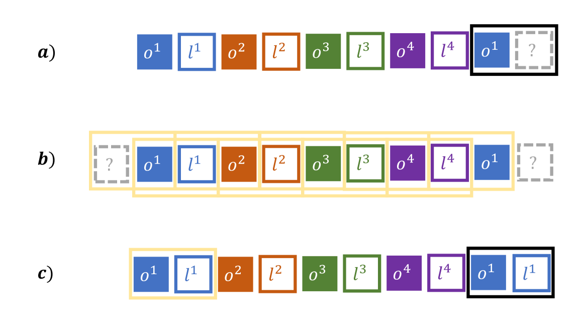
Let $X\in\mathbb{R}^{\mathcal{e}\times\mathcal{s}}$ be the input sequence data, where $\mathcal{e}$ is the dimension of each token embedded within a suitable latent space, and $\mathcal{s}$ is the number of tokens in the sequence. Each token is considered either an object, $o$, or label, $l$. Input $X$ consists of a sequences of multiple pairs of objects and labels. We say a pair of tokens is a contiguous sub-sequence of two column vectors from within $X$, consisting of one object token followed by one label token. For example, the $j$-th pair $X^{\prime}\in\mathbb{R}^{\mathcal{e}\times 2}$ consists of one object token $o^{j}\in\mathbb{R}^{\mathcal{e}}$ followed by one label token $l^{j}\in\mathbb{R}^{\mathcal{e}}$. Our input sequence $X$ will therefore consist of multiple pairs, and each pair may appear more than once. The final token of a sequence, denoted as $x_{\mathcal{s}}$, corresponds to the label token of the last pair, which itself has appeared at least once prior to this final instance in $X$. However, the true label token data of this final label token is replaced with the zero vector, and the network’s task is to correctly predict this true label token given the previous in-context instance of the tokens’ data (as illustrated in Figure 1a).

The token embeddings, representing objects and labels, follows Reddy (2024), where all token embeddings are drawn from similar statistical distributions. For every instance of a pair, label token embeddings comes from fixed vectors, whereas object token embeddings are constructed from combinations of fixed and random vectors. Each label token $l^{i}$ is an $\mathcal{e}$–dimensional vector $\mu_{l^{i}}$, whose components are i.i.d. sampled from a normal distribution having mean zero and variance $1/\mathcal{e}$. Each object token embedding, $o^{i}$, is given by

$$o^{i}:=\frac{\mu_{o^{i}}+\varepsilon\eta}{\sqrt{1+\varepsilon\varepsilon}},$$

where $\mu_{o^{i}}$, which is fixed across all instances in $X$ of the pair, and $\eta$, which is drawn randomly for each instance in $X$ of the pair, are $\mathcal{e}$–dimensional vectors whose components, like $\mu_{l^{i}}$, are i.i.d. sampled from a normal distribution having mean zero and variance $1/\mathcal{e}$. The variable $\varepsilon$ controls the inter-instance variability of objects and, in the following, is set to $0.1$ unless otherwise stated. This means that the final, tested instance of a pair has, as its object token, a slightly different appearance than the previous instance(s) seen in $X$ and is not a perfect match, where $\mu_{o^{i}}$ provides the commonality between these variations. Adding these variations makes the task less trivial and slightly more naturalistic.

We now show it is possible to perform ICL with such pairs in a single forward step of a one-layer associative memory network, written in the language of a single Transformer attention head (Vaswani et al., 2017). In Transformers, each attention head consists of learnt parameters – weight matrices $W^{q},W^{k}\in\mathbb{R}^{\mathcal{k}\times\mathcal{e}}$ and $W^{v}\in\mathbb{R}^{\mathcal{v}\times\mathcal{e}}$ – with which, when taken together with the input data sequence $X$, we calculate the queries $Q$, keys $K$, and values $V$ matrices using

$$Q=W^{q}X,\quad K=W^{k}X,\quad\text{and}\quad V=W^{v}X.$$

The values $\mathcal{k}$ and $\mathcal{v}$ are the reduced embedding dimensions for the attention operation (i.e., to facilitate multi-headed attention, etc.). Here we use $\mathcal{k}=\mathcal{v}$. As in the input data, $\mathcal{e}$ is the dimension of the unreduced embedding space of the tokens.

It is then useful to define the softmax function for matrix arguments. For a matrix $M\in\mathbb{R}^{\mathcal{c}\times\mathcal{r}}$, we write $t_{i}:=M[i,:]\in\mathbb{R}^{\mathcal{r}}$ for the $i$-th row and $t_{j}:=M[:,j]\in\mathbb{R}^{\mathcal{c}}$ for the $j$-th column. Then, we define the softmax function for a matrix $M$ as $\textsc{softmax}(M)[t_{i},t_{j}]:=\frac{\text{exp}(M[t_{i},t_{j}])}{\sum_{t}\text{exp}(M[t,t_{j}])}$, where $i$ and $j$ are the vector component indices. We use this to compute attention-based embeddings of the data $X$, denoted by $\tilde{X}$, as

$$\tilde{X}=\textsc{softmax}\left(\frac{1}{\sqrt{\mathcal{k}}}K^{T}Q\right)V,$$ (1)

in which we refer to the term $K^{T}Q$ as the scores $S\in\mathbb{R}^{\mathcal{s}\times\mathcal{s}}$. In Transformers and Transformer-based models such as LLMs, this new data $\tilde{X}$ is then recombined with data from other attention heads, before passing through a multi-layer perceptron. Layers of attention heads and multi-layer perceptrons are stacked atop one-another to perform increasingly sophisticated computations.

In our associative memory model, which we call Associative Memory for ICL (AMICL), we take inspiration from the transformations applied to the input data $X$ to create the basis of what can be considered (Ramsauer et al., 2021) as an associative memory update step in Equation 1. Instead of using parameterised values, we use a simple set of assignments for each token’s key, query, and value vectors. For all embedded tokens $i<\mathcal{s}$, we set $k_{i}=q_{i}=\frac{ax_{i-1}+x_{i}}{a+1}$ as the keys and queries, where lowercase Latin letters denote indexed column vectors, taken from the matrices that are denoted with uppercase Latin letters. For simplicity, we wrap the indices along the token sequence such that the first token, $x_{1}$, and the last token, $x_{\mathcal{s}}$, are used to generate the sub-sequence $(x_{\mathcal{s}},x_{1})$, i.e., we assign token index $0$ to $\mathcal{s}$. For token $\mathcal{s}$, with $x_{\mathcal{s}}$ as the token column vector, we set $q_{\mathcal{s}}=\frac{ax_{\mathcal{s}-1}+x_{\mathcal{s}}}{a+1}$ as the query and $k_{\mathcal{s}}$ as the zero vector, which acts as its key. For all tokens, the values column vector is equal to the token column vector, i.e., $v_{j}=x_{j}$. The value of $a$ can be any arbitrary positive real value, but, after testing within the range $[0,2]$, is set as $a=2$.

We then perform next token prediction using the universal associative memory framework (Millidge et al., 2022), which can be interpreted as a generalisation of Equation 1. In particular, Equation 1 in the universal associative memory framework has the form $\textsc{projection}(\textsc{separation}(\textsc{similarity}(K,Q)),V)$, where the similarity function is chosen as a scaled dot product, the separation function is chosen as a softmax, and the projection function is chosen as a product.

Intuitively, AMICL can be thought of as implementing the algorithm illustrated in Figure 1. First, we identify the final pair, where the final token, $x_{\mathcal{s}}$, which should be a label token, has been set to the zero vector (Figure 1a, where ‘?’ represents the unknown token data and other tokens’ data are shown); second, we consider all possible contiguous pairs in the context, e.g., $(x_{3},x_{4}),(x_{4},x_{5}),\dots$, without knowledge of their data, which we as designers know will correspond to pairs like, e.g., $(o^{2},l^{2}),(l^{2},o^{3}),\dots$ (Figure 1b, where each contiguous pair is enclosed by a yellow rectangle); third, we compare all of the contiguous pairs in the second step with the final pair identified in the first step (which we are attempting to ‘pattern complete’), and, upon seeing which context pair is most similar in final pair (in this example, $(o^{1},l^{1})$), complete the pattern appropriately by setting $x_{\mathcal{s}}=l^{1}$ (Figure 1c).

Figure 1: Depiction of the AMICL algorithm on label–object pairs, consisting of three steps: (a) consider the penultimate and final tokens as a ‘local pattern’ which has been ‘partially corrupted’ by the missing data in the final token, illustrated by the black rectangle enclosing this final pair; (b) search for matching, ‘complete local patterns’ by grouping all previous contiguous token pairs in the context, with each pair illustrated by a yellow rectangle enclosing the tokens; and (c) complete the final, corrupted local pattern based on matching to the nearest complete in-context pair, which in this case is $(o^{1},l^{1})$, so the final token data is assigned $l^{1}$.

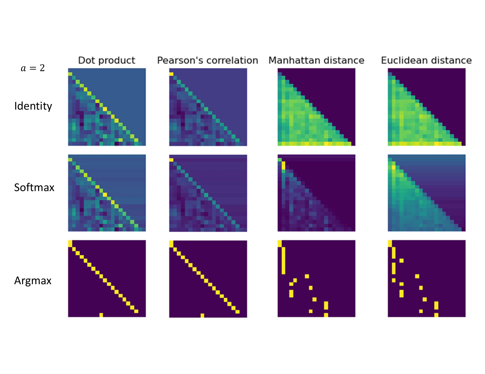
While setting $a=2$ and $\textsc{projection}=\textsc{identity}$, we tested all combinations of:

• $\textsc{similarity}\in\{\textsc{dot product},\textsc{pearson's correlation},\textsc{manhattan distance},\\ \textsc{euclidean distance}\}$; with

• $\textsc{separation}\in\{\textsc{identity},\textsc{softmax},\textsc{argmax}\}$.

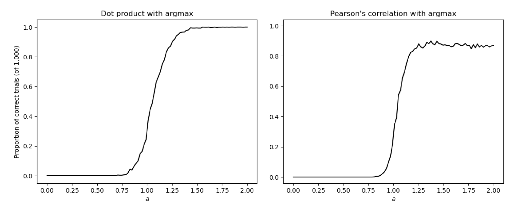
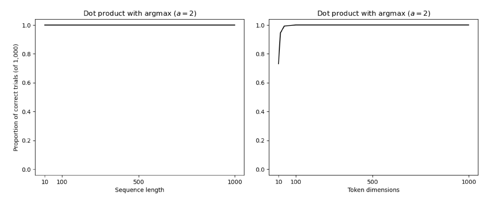
Manual inspection of the resulting attention matrices indicated that the dot product and pearson’s correlation similarity functions combined with the argmax separation function provided the cleanest ICL (see Figure 4 in Appendix A for an example). Varying the parameter $a$ between $0$ and $2$ for both combinations showed that using the dot product similarity with argmax separation function resulted in practically perfect ICL ability at $a\geq 1.5$ whereas using pearson’s correlation similarity with argmax separation function saturated at a performance level of $\sim 85\%$ accuracy for the ICL pairs task (see Figure 5 in Appendix A). Varying the token sequence length $\mathcal{s}$ between $10$ and $1,000$ shows no variation in performance; varying the embedding dimension of the tokens $\mathcal{e}$ between $10$ and $1,000$ showed that for $\mathcal{e}\geq 50$, the ICL task performance was practically perfect (see Figure 6 in Appendix A).

3 Residual attention streams in a two-layer Transformer

Following the path of information from the input to the queries, keys, and values in the AMICL model (Figure 2a), we can see that the queries $Q$ and keys $K$ flow from a shared function $f$ of the input $X$. Whereas, the values $V$ are given directly by the input $X$. Seen through the lens of the traditional self-attention mechanism, construction of the AMICL model in Section 2 can be interpreted as implying that creating the values $V$ in a way which more explicitly retains the prior input $X$ can facilitate ICL. Inspired by this, we introduce a residual connection between the values data of successive layers in the Transformer, which we call a residual values stream and, more generally, a residual attention stream applied to values (Figure 2b).

Figure 2: Partial diagrams of (a) the AMICL model and (b) our residual attention stream architecture with two Transformer layers, $n$ and $n-1$, shown here implemented for values (the added residual is shown in green). Boxes represent variables. Full arrows represent functions, with overlaid circles indicating relevant variables or functions (no circle is used for the identity function). Dotted arrows represent functions and variables omitted in the diagram for space.

As an alternative source of intuition, one can consider the informal interpretation of self-attention as consisting of: queries ‘asking each token a question about other tokens’; keys ‘responding to each token with the answer to the queries’ questions’, i.e., they align with or ‘attend to’ the queries; and values giving the (weighted) answers to those questions, which are operationalised as small additions to the current token vectors. Within this informal conceptual model, we can consider our residual attention streams as retaining additional ‘look-back’ information in the answers.

Our residual attention stream also generates additional gradient signals during training, which could themselves be beneficial for the network to develop ICL capabilities. We therefore also test the same residual stream architecture, separately, for queries and keys. In principle, it is also possible to apply the residual stream architecture to combinations of queries, keys, and values. But, to maintain a stronger connection to the AMICL model, we focus on testing the residual value stream separately, as well as the keys and queries, again separately, for comparison.

We train classic and modified versions of a two-layer Transformer on the same task described in Section 2. The common architectural features between the two versions consist of two single-head attention layers followed by a three-layer multi-layer perceptron with 128 ReLU neurons followed by a softmax layer to give probabilities over the $\mathcal{l}$ labels. The network is trained with the same task as the AMICL model, using the cross-entropy loss between the predicted and actual final label in token $x_{\mathcal{s}}$. Within the modified architecture, we add the first attention head’s queries, keys, or values to the second attention head’s queries, keys, or values, respectively. More formally, in our modified version of the Transformer architecture, we calculate the first attention layer as

$$Q_{1}=W^{q}_{1}X,\quad K_{1}=W^{k}_{1}X,\quad\text{and}\quad V_{1}=W^{v}_{1}X,$$

and then, in the second attention layer, for a residual queries stream we calculate

$$Q_{2}=W^{q}_{2}X+Q_{1},\quad K_{2}=W^{k}_{2}X,\quad\text{and}\quad V_{2}=W^{v}_{2}X,$$

or for a residual keys stream we calculate

$$Q_{2}=W^{q}_{2}X,\quad K_{2}=W^{k}_{2}X+K_{1},\quad\text{and}\quad V_{2}=W^{v}_{2}X,$$

or for a residual values stream (shown in Figure 2b) we calculate

$$Q_{2}=W^{q}_{2}X,\quad K_{2}=W^{k}_{2}X,\quad\text{and}\quad V_{2}=W^{v}_{2}X+V_{1}.$$

As in Reddy (2024), while we train on the originally-described ICL task, we create supplemental tasks which are not used for training but rather act as proxy measurements of progress for different computational strategies for completing the task: training data memorisation and ICL capability generalisation. Namely, these supplemental tasks are:

• In-weights (IW): a series of object–label pairs is presented where the final pair is not found within the prior context but is present in the training data;

• In-context (IC): a series of novel object–label pairs, not seen in the training data (i.e., an entirely re-drawn set of $\mu_{o^{i}}$ and $\mu_{l^{i}}$ values) but following exactly the same statistical structure, is presented; and

• In-context 2 (IC2): a series of object–label pairs are presented, where the objects are found in the training data but have been assigned new labels (i.e., the objects retain their $\mu_{o^{i}}$ values but the labels have their $\mu_{l^{i}}$ values re-drawn).

Figure 3: Accuracies and losses for the Test, IW, IC, and IC2 tasks over training time for the classic (unmodified) network and residual queries, keys, and values stream networks. Dark lines represent means, light lines represent individual trials.

The reduced embedding dimensions of the attention operation are both set to 128, i.e., $\mathcal{k,v=128}$. Each network architecture was trained on four random seeds, with a batch size of 128, vanilla stochastic gradient descent, and a learning rate of 0.01.

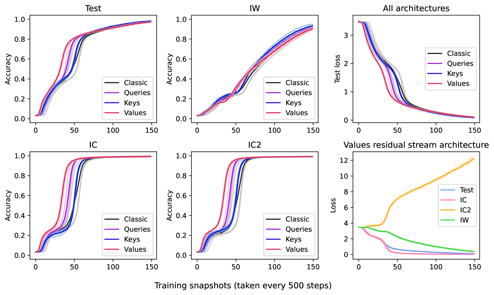
Figure 3 shows the accuracies for the task being trained (Test) and the three supplemental tasks (IW, IC, and IC2) for each architecture. It also shows the Test loss for all architectures and all loses for the values residual stream architecture. For our residual attention stream modifications, we observe a general leftward shift in all but the IW task, with the value residual stream architecture showing the largest shift. The IW task also shows a slower learning rate, which can be attributed to the relative difficulty of the network memorising the training data.

To quantify these shifts, we report statistics in Table 1 of when the first training snapshots we recorded reached an accuracy threshold of $>0.95$. We find the values stream networks perform best, reaching the same level of accuracy as the classic (unmodified) networks with $\sim 24\%$ fewer training steps. The same result is also seen at lower thresholds (see Tables 3 and 4 in Appendix B for thresholds of $0.5$ and $0.9$, respectively). We also performed t-tests at the $0.95$ accuracy threshold, which showed significant differences between the performance of the classic (unmodified) network and the residual queries and values stream networks on the IC and IC2 tasks ($p<0.01$, $t<-3.9$), but not between the classic and residual keys stream networks ($p>0.39$, $t>-1.0$). The residual values stream networks also perform significantly better ($p<0.03$, $t<-3.0$) than all other networks on both the IC and IC2 task, except the residual queries stream network for the IC task ($p=0.06$, $t=-2.33$).

Table 1: Mean $\pm$ standard deviation of training snapshot number where accuracy first exceeded $0.95$ for the IC and IC2 tasks in the classic (unmodified), and residual queries, keys, and values stream networks. Fastest training times are bolded.

	Classic	Queries (ours)	Keys (ours)	Values (ours)
IC	64.5 $\pm$ 5.12	52.5 $\pm$ 1.5	61.75 $\pm$ 0.83	49.0 $\pm$ 2.12
IC2	63.25 $\pm$ 4.15	51.75 $\pm$ 1.92	61.25 $\pm$ 0.83	47.75 $\pm$ 1.3

4 Residual value streams in a small language model

To provide an initial indication as to whether the benefit for ICL performance seen in Section 3 scales to larger models and naturalistic data, we also test the residual value stream architecture by training small LMs. The Transformer-based model contains approximately 8 million parameters spread over eight layers, each with 16 attention heads. The context window is 256 tokens long and dimension of the model is $256$. Next-token prediction is trained for three epochs on the Tiny Stories dataset, such that they can generate simple and short children’s stories (Eldan & Li, 2023). Each network architecture was trained in three separate instances, using different random seeds for each instance but controlling for randomness between architectures by re-using the same set of seeds for the two architectures.

We implement the residual value stream in a naïve way: in each but the first layer, the values of each attention head receives an additional input of the values from the attention head with the same index in the previous layer. Although there are alternative implementations of such residual streams, we chose a naïve and straightforward approach to provide an initial indication of the potential scalability of this architectural change and to not alter the number of learnt parameters between the networks.

The residual values stream networks achieved $1.65\pm 0.05$ training loss and $1.55\pm 0.01$ validation loss, slightly lower than the training and validation losses for the classic networks, which were $1.67\pm 0.05$ and $1.56\pm 0.01$, respectively. Measured by wall clock computation time, the residual values stream networks also took slightly longer to train, $30.18\pm 0.49$ hours compared to $29.12\pm 0.40$ hours for the classic networks. This additional computation time is attributable to the additional gradient computations required by the 16 additional residual streams connecting the attention head values at each but the first layer.

As a proxy evaluation of the ICL ability of each model in natural language, we utilise a simple indirect object identification (IOI) task. In natural language, a direct object is the noun that receives the action of the verb and an indirect object is a noun which receives the direct object, e.g., in the sentence “A passed B the ball”: “passed” is the verb; “A” is the subject; “the ball” is the direct object; and “B” is the indirect object. In the IOI task, we test for correct completion of sentences like “When A and B were playing with a ball, A passed the ball to”, where “ B” is the indirect object and is considered the correct completion.

GPT-2 Small can perform instances of the IOI task, and the circuit responsible for this ability has been identified (Wang et al., 2023). As shown in this section, our small LMs have some measurable ability to complete instances of this task, and so we use this to compare the performance of the classic (unmodified) and residual value stream architectures.

For the IOI task, we tested the following sentences:

1. “When John and Mary went to the shops, $\ast$ gave the bag to”, where $\ast$ was either “John” or “Mary”, with correct completions “ Mary” and “ John”, respectively.

2. “When Tom and James went to the park, $\ast$ gave the ball to”, where $\ast$ was either “Tom” or “James”, with correct completions “ James” and “ Tom”, respectively.

3. “When Dan and Emily went to the shops, $\ast$ gave an apple to”, where $\ast$ was either “Dan” or “Emily”, with correct completions “ Emily” and “ Dan”, respectively.

4. “After Sam and Amy went to the park, $\ast$ gave a drink to”, where $\ast$ was either “Sam” or “Amy”, with correct completions “ Amy” and “ Sam”, respectively.

For each sentence and variation thereof (swapping the identities of the subject and indirect object, as indicated by the $\ast$ symbol above), we recorded the next token probabilities of the correct and incorrect names. As summarised in Table 2, we find the classic networks are much less capable than the residual values stream networks – across the four sentences, the classic networks correctly identify the indirect object with a probability of $\sim 7\%$ while the residual values stream networks do so with a probability of $\sim 41\%$, a $\sim 5.9\times$ improvement. Similarly, the classic networks more regularly mistake the subject for the indirect object with a probability of $\sim 5\%$ while the residual values stream networks do so with a probability of $\sim 3\%$, a $\sim 0.6\times$ reduction.

Table 2: Mean $\pm$ standard deviation probabilities (%) of correct and incorrect responses to each sentence for the IOI task for the classic (unmodified) and residual values stream networks. Best scores are bolded.

Classic	Sentence 1	Sentence 2	Sentence 3	Sentence 4
Correct (higher is better)	11.73 $\pm$ 15.62	11.88 $\pm$ 9.09	3.83 $\pm$ 6.09	1.54 $\pm$ 2.31
Incorrect (lower is better)	6.93 $\pm$ 5.70	7.99 $\pm$ 9.52	0.51 $\pm$ 0.66	4.86 $\pm$ 8.35
Residual values stream (ours)	Sentence 1	Sentence 2	Sentence 3	Sentence 4
Correct (higher is better)	42.89 $\pm$ 10.58	43.44 $\pm$ 14.45	49.24 $\pm$ 9.89	28.56 $\pm$ 5.92
Incorrect (lower is better)	5.68 $\pm$ 3.76	6.8 $\pm$ 10.40	0.03 $\pm$ 0.03	0.18 $\pm$ 0.15

5 Discussion

Our study builds upon the understanding of ICL in Transformer models by exploring connections to associative memory models from computational neuroscience. We introduced AMICL, an associative memory model that performs ICL using an approach akin to a single-layer Transformer attention head but with an implied residual stream from the inputs to the values. Inspired by this, we proposed a novel residual stream architecture in Transformers, where information flows directly between attention heads. We demonstrate this in a two-layer Transformer, showing increased efficiency in learning on an ICL classification task. Moreover, by extrapolating this architecture to a small Transformer-based LM, we illustrated enhanced ICL capabilities are possible on a larger and more naturalistic scale.

Our results offer potential insights for neural network design and our understanding of biological cognition:

• Neural network architecture. The simplicity of our biologically-inspired architectural modification, attention residual streams, provides a promising extension for designing more adaptive Transformer models. Given one can interpret this change as providing additional shared workspaces across model layers (in the form of the additional residual streams), our results can also be viewed as supporting cognitive functional specialisation and modularisation as being both natural and commonplace in neural systems (Kaiser & Hilgetag, 2006; Chen et al., 2013), which is also seen in cases of highly distributed representations (Voitov & Mrsic-Flogel, 2022), of which natural language appears no exception (Mikolov et al., 2013; Hernandez et al., 2024).

• Biological cognition. Drawing parallels between artificial networks and cognitive neuroscience theories contributes to a deeper understanding of memory systems in biological entities. As we have shown by our AMICL model, the associative memory framework is capable of ICL in a single layer, with an implied ‘skip connection’ present between the input and the values. This suggests that similar types of connections may analogously exist in biological networks to adapt and generalize from limited exposure. For instance, associative memory is often related to the hippocampal formation (Amit, 1989), an area in the brain important for memory and learning. An open question in this area of neuroscience is what the computational role of observed skip connections are. In particular, while some information in the hippocampus goes directly from area CA3 to CA1, another area – CA2 – is often skipped, but does receive input from CA3, which it then passes on to CA1 (Cui et al., 2013). This is interesting not just anatomically, but also functionally, since CA2 is considered responsible for specialised tasks and context-switching (Dudek et al., 2016; Robert et al., 2018). Whether our AMICL model or residual attention stream modification can be considered analogous to skip connections witnessed in the hippocampus remains to be studied. However, it offers a promising window, e.g., one could now study the effects of changing the number and quality of residual attention streams, to test whether connection types or relative proportions similar to that seen in the hippocampus also show improved performance (for some types of data or tasks).

In establishing an additional potential mechanistic link between associative memory frameworks and ICL tasks, this work builds upon the broader biologically-inspired interpretation of Transformer attention mechanisms (Ramsauer et al., 2021). Indeed, Zhao (2023) conjectures that LLMs performing ICL do so using an associative memory model which performs a kind of pattern-completion using provided context tokens, conditioned by the learnt LLM parameters. Using this perspective, Zhao (2023) constructs different token sequences to be used as contexts to prepend onto the same final token sequence representing the tested task. By actively choosing context tokens which more ‘closely’ resemble the final tokens the LLM is being tested with, the LLM shows improved task performance, presumably by utilising the increased relevancy of the context tokens for ICL. This perspective is further developed in Jiang et al. (2024), who show how LLMs can be ‘hijacked’ by purposeful use of contexts with particular semantics. When LLMs such as Gemma-2B-IT and LLaMA-7B are given the context of “The Eiffel Tower is in the city of”, they successfully predict the next token as “ Paris”. However, Jiang et al. (2024) demonstrate that prepending the context with the sentence “The Eiffel Tower is not in Chicago.” a sufficient number of times, these LLMs incorrectly predict the next token as “ Chicago”. We may interpret these prepended data as acting (crudely) as ‘distractors’, and in the associative memory sense as causing an over-activation of competing memory items which interferes with accurate task performance.

Beyond associative memory, we also note potential connections with other computational neuroscience models. In particualr, we observe that our model, AMICL, has some connection to successor representation, particularly $\gamma$–models, where the parameter $a$ is somewhat similar to the $\gamma$ parameter (Janner et al., 2020). Interestingly, a variant of the temporal context model, which was recently compared to ICL in LLMs (Ji-An et al., 2024), can be considered equivalent (Gershman et al., 2012) to estimating the successor representation using the temporal difference method from reinforcement learning (Sutton, 1988). This suggests that parametrising our residual stream architecture, e.g., by providing weighted sums of previous-layer values (where the weights act like $\gamma$ variables) across multiple attention heads instead of the data from a single attention head with the same index, and training these parameters using a reinforcement learning algorithm, could provide further enhancements.

Future work may seek to more deeply understand our results in the context of varying the structure and order of context tokens – in associative memory networks, and during inference and training of LLMs. Along these lines, Russin et al. (2024) recently showed that LLMs and Transformers exhibit similar improvements as seen in humans on tasks with and without rule-like structures, depending on the order and organisation of context and training tokens. In particular, ICL performance improved when context tokens appeared in semantically-relevant ‘chunks’ or ‘blocks’, as seen in humans when completing tasks with rule-like structures. Whereas, when training samples were interleaved, Transformers saw performance improvements (as measured by the extent to which the network rote-learnt training examples), similar to humans completing tasks lacking rule-like structures.

The performance improvements from introducing a residual values stream suggests that ICL can be thought of as an associative process where continuous information reinforcement enhances model memory, efficiency, and prediction accuracy on novel data. Nonetheless, this raises several questions. Firstly, more comprehensive testing on varied datasets and different scales of language models can address whether the improvements we observed generalise beyond our specific tasks and data setups. Further, it remains to be clarified whether similar benefits manifest when dealing with other natural language processing tasks, such as sentiment analysis or translation, or whether there exist any trade-offs between ICL and other abilities. Additionally, while these initial results present a compelling case for testing attention residual streams in larger models, further exploration of optimisation parameter settings for such architectures would strengthen understanding. Quantitative studies on computation cost versus accuracy improvements will also better-inform model architecture design and selection for deployment in real-world scenarios, as well as potential competition between learning flexibility and task accuracy.

In conclusion, this research demonstrates potential conceptual and practical advancements in enhancing Transformers’ adaptive capabilities through a biologically-inspired mechanism. By bridging neural computational principles with associative memory insights, we offer new directions for research into more intelligent and dynamic models, with potential improvements for LLMs. Our associative memory model and Transformer architecture not only bolsters existing computational frameworks, but also offers fertile ground for computational neuroscientists to analyse the computational role of skip connections in memory systems. As we progress, these interdisciplinary approaches may ultimately yield richer cognitive models that parallel, or even emulate, biological intelligence.

Acknowledgments

This effort was supported by the Cornell University SciAI Center. T.B. and C.E. were funded by the Office of Naval Research (ONR), under Grant Number N00014-23-1-2729. T.F. was supported by JSPS KAKENHI no. JP23H05476. T.B. thanks Gautam Reddy for code sharing.

Code availability

Code used to produce these results can be found at https://github.com/tfburns/AMICL-and-residual-attention-streams.

Appendix

Appendix A Extended figures

Figure 4: Attention matrices for label–object pairs in AMICL, using different similarity and separation functions with $a=2$.

Figure 5: Proportion of correct trials, tested over $1,000$ trials for values between $a=0$ and $a=2$ in AMICL for label–object pairs using the dot product (left) and Pearson’s correlation (left) similarity with the argmax separation function.

Figure 6: Proportion of correct trials, tested over $1,000$ trials for varying the values of the sequence length ($\mathcal{s}$, left) and token dimensions ($\mathcal{e}$, right) between $10$ and $1,000$ in AMICL for label–object pairs using $a=2$ with the dot product similarity function and argmax separation function.

Appendix B Extended tables

Table 3: Mean $\pm$ standard deviation of training snapshot number where accuracy first exceeded $0.5$ for the IC and IC2 tasks in the classic (unmodified), and residual queries, keys, and values stream networks.

	Classic	Queries (ours)	Keys (ours)	Values (ours)
IC	51.0 $\pm$ 4.24	41.5 $\pm$ 2.29	49.75 $\pm$ 0.43	32.75 $\pm$ 0.83
IC2	51.5 $\pm$ 4.39	41.5 $\pm$ 1.66	49.25 $\pm$ 0.83	33.25 $\pm$ 1.09

Table 4: Mean $\pm$ standard deviation of training snapshot number where accuracy first exceeded $0.9$ for the IC and IC2 tasks in the classic (unmodified), and residual queries, keys, and values stream networks.

	Classic	Queries (ours)	Keys (ours)	Values (ours)
IC	59.25 $\pm$ 4.49	48.25 $\pm$ 1.48	57.5 $\pm$ 0.5	42.25 $\pm$ 1.3
IC2	59.0 $\pm$ 4.53	48.0 $\pm$ 1.87	57.25 $\pm$ 0.83	42.0 $\pm$ 0.71

Appendix C Notation and abbreviations tables

A comprehensive list of all notations and abbreviations used in this paper is provided in the tables below.

Abbreviations
LLMs	large language models
ICL	in-context learning
LMs	langauge models
i.i.d.	independent and identically distributed
IW	in-weight
IC	in-context
IC2	in-context 2
IOI	indirect object identification
CA1, CA2, CA3	cornu Ammonis 1, 2, 3

Variables
$X_{i}$	The input sequence data $X_{i}\in\mathbb{R}^{\mathcal{e}\times\mathcal{s}}$, with $\mathcal{s}$ column vectors, corresponding to the token embeddings, each of dimension $\mathcal{e}$. Where the subscript $i$ is present, this denotes the data is taken from the $i$–th Transformer layer, i.e., the residual stream data.
$x_{i}$	A token embedding $x_{i}\in\mathbb{R}^{\mathcal{e}}$, where the subscript $i$ denotes the column position in the input sequence $X$.
$x_{\mathcal{s}}$	The token embedding $x_{i}\in\mathbb{R}^{\mathcal{e}}$ of the final column, i.e., the final token, in the input sequence $X$.
$o^{i}$	An object token embedding $o^{i}\in\mathbb{R}^{\mathcal{e}}$, where the superscript $i$ identifies the object–label identity.
$l^{i}$	A label token embedding $l^{i}\in\mathbb{R}^{\mathcal{e}}$, where the superscript $i$ identifies the object–label identity.
$\mu_{i}$	A vector $\mu_{i}\in\mathbb{R}^{\mathcal{e}}$ whose components are i.i.d. sampled from a normal distribution having mean zero and variance $1/\mathcal{e}$. Used for constructing the token embeddings of object or label $i$, where for each object, $o^{i}$, and label, $l^{i}$, the vector $\mu_{i}$ is fixed.
$\varepsilon$	A fixed real number $\varepsilon\in\mathbb{R}$ which controls the inter-instance variability of objects, and is set to $0.1$ unless stated otherwise.
$\eta$	A vector $\eta\in\mathbb{R}^{\mathcal{e}}$ whose components are i.i.d. sampled from a normal distribution having mean zero and variance $1/\mathcal{e}$. Redrawn and used for adding inter-instance variability in the construction of each object token embedding.
$W^{q}_{i},W^{k}_{i}$	Query and key weight matrices $W^{q},W^{k}\in\mathbb{R}^{\mathcal{k}\times\mathcal{e}}$, respectively, of the $i$–th Transformer layer.
$W^{v}_{i}$	Value weight matrix $W^{v}\in\mathbb{R}^{\mathcal{v}\times\mathcal{e}}$ of the $i$–th Transformer layer.
$Q_{i}$	Queries matrix $Q\in\mathbb{R}^{\mathcal{k}\times\mathcal{s}}$ of the $i$–th Transformer layer, calculated using $W^{q}_{i}$ and $X_{i}$.
$K_{i}$	Keys matrix $K\in\mathbb{R}^{\mathcal{k}\times\mathcal{s}}$ of the $i$–th Transformer layer, calculated using $W^{k}_{i}$ and $X_{i}$.
$V_{i}$	Values matrix $V\in\mathbb{R}^{\mathcal{v}\times\mathcal{s}}$ of the $i$–th Transformer layer, calculated using $W^{v}_{i}$ and $X_{i}$.
$S_{i}$	The scores matrix, $S_{i}\in\mathbb{R}^{\mathcal{s}\times\mathcal{s}}$, which is equal to $K_{i}^{T}Q_{i}$.
$q_{i}$	A queries column vector, $q_{i}\in\mathbb{R}^{\mathcal{k}}$, where the subscript $i$ denotes the column position in the queries matrix $Q$.
$k_{i}$	A keys column vector, $k_{i}\in\mathbb{R}^{\mathcal{k}}$, where the subscript $i$ denotes the column position in the keys matrix $K$.
$v_{i}$	A values column vector, $v_{i}\in\mathbb{R}^{\mathcal{v}}$, where the subscript $i$ denotes the column position in the values matrix $V$.

Dimensions
$\mathcal{e}$	Dimensionality $\mathcal{e}\in\mathbb{N}^{+}$ of each token embedding.
$\mathcal{s}$	Number of tokens $\mathcal{s}\in\mathbb{N}^{+}$ in the input sequence data $X$.
$\mathcal{k}$	Reduced token embedding dimension $\mathcal{k}\in\mathbb{N}^{+}$ for keys and queries in the attention operation.
$\mathcal{v}$	Reduced token embedding dimension $\mathcal{v}\in\mathbb{N}^{+}$ for values in the attention operation.
$\mathcal{l}$	Number of unique labels $\mathcal{l}\in\mathbb{N}^{+}$ in the input sequence data $X$.

References

- Amari (1972) Shun’ichi Amari. Learning patterns and pattern sequences by self-organizing nets of threshold elements. IEEE Transactions on Computers, C-21(11):1197–1206, 1972. doi: 10.1109/T-C.1972.223477.
- Amit (1989) Daniel J Amit. Modeling brain function: The world of attractor neural networks. Cambridge university press, 1989.
- Amit (1990) Daniel J Amit. Attractor neural networks and biological reality: associative memory and learning. Future Generation Computer Systems, 6(2):111–119, 1990.
- Boorman et al. (2021) Erie D Boorman, Sarah C Sweigart, and Seongmin A Park. Cognitive maps and novel inferences: a flexibility hierarchy. Current Opinion in Behavioral Sciences, 38:141–149, 2021. ISSN 2352-1546. doi: https://doi.org/10.1016/j.cobeha.2021.02.017. URL https://www.sciencedirect.com/science/article/pii/S2352154621000395. Computational cognitive neuroscience.
- Bricken & Pehlevan (2021) Trenton Bricken and Cengiz Pehlevan. Attention approximates sparse distributed memory. In A. Beygelzimer, Y. Dauphin, P. Liang, and J. Wortman Vaughan (eds.), Advances in Neural Information Processing Systems, 2021. URL https://openreview.net/forum?id=WVYzd7GvaOM.
- Brown et al. (2020) Tom Brown, Benjamin Mann, Nick Ryder, Melanie Subbiah, Jared D Kaplan, Prafulla Dhariwal, Arvind Neelakantan, Pranav Shyam, Girish Sastry, Amanda Askell, et al. Language models are few-shot learners. Advances in neural information processing systems, 33:1877–1901, 2020.
- Burns (2024) Thomas F Burns. Semantically-correlated memories in a dense associative model. In Ruslan Salakhutdinov, Zico Kolter, Katherine Heller, Adrian Weller, Nuria Oliver, Jonathan Scarlett, and Felix Berkenkamp (eds.), Proceedings of the 41st International Conference on Machine Learning, volume 235 of Proceedings of Machine Learning Research, pp. 4936–4970. PMLR, 21–27 Jul 2024. URL https://proceedings.mlr.press/v235/burns24a.html.
- Burns & Fukai (2023) Thomas F Burns and Tomoki Fukai. Simplicial hopfield networks. In The Eleventh International Conference on Learning Representations, 2023. URL https://openreview.net/forum?id=_QLsH8gatwx.
- Burns et al. (2022) Thomas F Burns, Tatsuya Haga, and Tomoki Fukai. Multiscale and extended retrieval of associative memory structures in a cortical model of local-global inhibition balance. eNeuro, 9(3), 2022. doi: 10.1523/ENEURO.0023-22.2022. URL https://www.eneuro.org/content/9/3/ENEURO.0023-22.2022.
- Buzsáki (2010) György Buzsáki. Neural syntax: Cell assemblies, synapsembles, and readers. Neuron, 68(3):362–385, 2010. ISSN 0896-6273. doi: https://doi.org/10.1016/j.neuron.2010.09.023. URL https://www.sciencedirect.com/science/article/pii/S0896627310007658.
- Chen et al. (2013) Yuhan Chen, Shengjun Wang, Claus C Hilgetag, and Changsong Zhou. Trade-off between multiple constraints enables simultaneous formation of modules and hubs in neural systems. PLoS Comput. Biol., 9(3):e1002937, March 2013.
- Cohen & Kahana (2022) Rivka T Cohen and Michael Jacob Kahana. A memory-based theory of emotional disorders. Psychological Review, 129(4):742, 2022.
- Cui et al. (2013) Zhenzhong Cui, Charles R Gerfen, and W Scott Young 3rd. Hypothalamic and other connections with dorsal ca2 area of the mouse hippocampus. Journal of comparative neurology, 521(8):1844–1866, 2013.
- Dalmaz et al. (2022) Onat Dalmaz, Mahmut Yurt, and Tolga Çukur. Resvit: residual vision transformers for multimodal medical image synthesis. IEEE Transactions on Medical Imaging, 41(10):2598–2614, 2022.
- Duan et al. (2023) Hanyu Duan, Yixuan Tang, Yi Yang, Ahmed Abbasi, and Kar Yan Tam. Exploring the relationship between in-context learning and instruction tuning, 2023. URL https://arxiv.org/abs/2311.10367.
- Dudek et al. (2016) Serena M Dudek, Georgia M Alexander, and Shannon Farris. Rediscovering area ca2: unique properties and functions. Nature Reviews Neuroscience, 17(2):89–102, 2016.
- Eldan & Li (2023) Ronen Eldan and Yuanzhi Li. Tinystories: How small can language models be and still speak coherent english?, 2023. URL https://arxiv.org/abs/2305.07759.
- Elhage et al. (2021) Nelson Elhage, Neel Nanda, Catherine Olsson, Tom Henighan, Nicholas Joseph, Ben Mann, Amanda Askell, Yuntao Bai, Anna Chen, Tom Conerly, et al. A mathematical framework for transformer circuits. Transformer Circuits Thread, 1(1):12, 2021.
- Gershman et al. (2012) Samuel J Gershman, Christopher D Moore, Michael T Todd, Kenneth A Norman, and Per B Sederberg. The successor representation and temporal context. Neural Computation, 24(6):1553–1568, 2012.
- Goel & Dolan (2000) Vinod Goel and Raymond J. Dolan. Anatomical Segregation of Component Processes in an Inductive Inference Task. Journal of Cognitive Neuroscience, 12(1):110–119, 01 2000. ISSN 0898-929X. doi: 10.1162/08989290051137639. URL https://doi.org/10.1162/08989290051137639.
- Hebb (1949) Donald Olding Hebb. The organization of behavior: A neuropsychological theory. Wiley, 1949.
- Hernandez et al. (2024) Evan Hernandez, Arnab Sen Sharma, Tal Haklay, Kevin Meng, Martin Wattenberg, Jacob Andreas, Yonatan Belinkov, and David Bau. Linearity of relation decoding in transformer language models. In The Twelfth International Conference on Learning Representations, 2024. URL https://openreview.net/forum?id=w7LU2s14kE.
- Hopfield (1982) John J Hopfield. Neural networks and physical systems with emergent collective computational abilities. Proceedings of the National Academy of Sciences, 79(8):2554–2558, 1982. doi: 10.1073/pnas.79.8.2554. URL https://www.pnas.org/doi/abs/10.1073/pnas.79.8.2554.
- Howard et al. (2005) Marc W Howard, Mrigankka S Fotedar, Aditya V Datey, and Michael E Hasselmo. The temporal context model in spatial navigation and relational learning: toward a common explanation of medial temporal lobe function across domains. Psychological review, 112(1):75, 2005.
- Huang et al. (2023) Zhongzhan Huang, Pan Zhou, Shuicheng YAN, and Liang Lin. Scalelong: Towards more stable training of diffusion model via scaling network long skip connection. In Thirty-seventh Conference on Neural Information Processing Systems, 2023. URL https://openreview.net/forum?id=0N73P8pH2l.
- Janner et al. (2020) Michael Janner, Igor Mordatch, and Sergey Levine. Gamma-models: Generative temporal difference learning for infinite-horizon prediction. In H. Larochelle, M. Ranzato, R. Hadsell, M.F. Balcan, and H. Lin (eds.), Advances in Neural Information Processing Systems, volume 33, pp. 1724–1735. Curran Associates, Inc., 2020. URL https://proceedings.neurips.cc/paper_files/paper/2020/file/12ffb0968f2f56e51a59a6beb37b2859-Paper.pdf.
- Ji-An et al. (2024) Li Ji-An, Corey Y. Zhou, Marcus K. Benna, and Marcelo G. Mattar. Linking in-context learning in transformers to human episodic memory, 2024. URL https://arxiv.org/abs/2405.14992.
- Jiang et al. (2024) Yibo Jiang, Goutham Rajendran, Pradeep Ravikumar, and Bryon Aragam. Do llms dream of elephants (when told not to)? latent concept association and associative memory in transformers, 2024. URL https://arxiv.org/abs/2406.18400.
- Juliani et al. (2022) Arthur Juliani, Ryota Kanai, and Shuntaro Sasai Sasai. The perceiver architecture is a functional global workspace. In Proceedings of the Annual Meeting of the Cognitive Science Society, volume 44, 2022.
- Kaiser & Hilgetag (2006) Marcus Kaiser and Claus C Hilgetag. Nonoptimal component placement, but short processing paths, due to long-distance projections in neural systems. PLoS Comput. Biol., 2(7):e95, July 2006.
- Khona & Fiete (2022) Mikail Khona and Ila R Fiete. Attractor and integrator networks in the brain. Nature Reviews Neuroscience, 23(12):744–766, 2022.
- Kozachkov et al. (2022) Leo Kozachkov, Ksenia V. Kastanenka, and Dmitry Krotov. Building Transformers from neurons and astrocytes. bioRxiv, 2022. doi: 10.1101/2022.10.12.511910. URL https://www.biorxiv.org/content/early/2022/10/15/2022.10.12.511910.
- Levi et al. (2024) Amir Levi, Noam Aviv, and Eran Stark. Learning to learn: Single session acquisition of new rules by freely moving mice. PNAS Nexus, 3(5):pgae203, 05 2024. ISSN 2752-6542. doi: 10.1093/pnasnexus/pgae203. URL https://doi.org/10.1093/pnasnexus/pgae203.
- Li et al. (2023) Yingcong Li, Muhammed Emrullah Ildiz, Dimitris Papailiopoulos, and Samet Oymak. Transformers as algorithms: Generalization and stability in in-context learning. In Andreas Krause, Emma Brunskill, Kyunghyun Cho, Barbara Engelhardt, Sivan Sabato, and Jonathan Scarlett (eds.), Proceedings of the 40th International Conference on Machine Learning, volume 202 of Proceedings of Machine Learning Research, pp. 19565–19594. PMLR, 23–29 Jul 2023. URL https://proceedings.mlr.press/v202/li23l.html.
- Little (1974) William A Little. The existence of persistent states in the brain. Mathematical Biosciences, 19(1):101–120, 1974. ISSN 0025-5564. doi: https://doi.org/10.1016/0025-5564(74)90031-5. URL https://www.sciencedirect.com/science/article/pii/0025556474900315.
- Lohnas et al. (2015) Lynn J Lohnas, Sean M Polyn, and Michael J Kahana. Expanding the scope of memory search: Modeling intralist and interlist effects in free recall. Psychological review, 122(2):337, 2015.
- Lorente de Nó (1938) Rafael Lorente de Nó. Analysis of the activity of the chains of internuncial neurons. Journal of Neurophysiology, 1(3):207–244, 1938.
- Lynch & Sermanet (2021) Corey Lynch and Pierre Sermanet. Language conditioned imitation learning over unstructured data, 2021. URL https://arxiv.org/abs/2005.07648.
- Mansouri et al. (2020) Farshad Alizadeh Mansouri, David J Freedman, and Mark J Buckley. Emergence of abstract rules in the primate brain. Nature Reviews Neuroscience, 21(11):595–610, 2020.
- McCulloch & Pitts (1943) Warren S McCulloch and Walter Pitts. A logical calculus of the ideas immanent in nervous activity. The bulletin of mathematical biophysics, 5:115–133, 1943.
- Mikolov et al. (2013) Tomas Mikolov, Ilya Sutskever, Kai Chen, Greg Corrado, and Jeffrey Dean. Distributed representations of words and phrases and their compositionality, 2013. URL https://arxiv.org/abs/1310.4546.
- Miller & Cohen (2001) Earl K Miller and Jonathan D Cohen. An integrative theory of prefrontal cortex function. Annual review of neuroscience, 24(1):167–202, 2001.
- Millidge et al. (2022) Beren Millidge, Tommaso Salvatori, Yuhang Song, Thomas Lukasiewicz, and Rafal Bogacz. Universal hopfield networks: A general framework for single-shot associative memory models. In International Conference on Machine Learning, pp. 15561–15583. PMLR, 2022.
- Mirchandani et al. (2023) Suvir Mirchandani, Fei Xia, Pete Florence, Brian Ichter, Danny Driess, Montserrat Gonzalez Arenas, Kanishka Rao, Dorsa Sadigh, and Andy Zeng. Large language models as general pattern machines, 2023. URL https://arxiv.org/abs/2307.04721.
- Nakano (1972) Kaoru Nakano. Associatron-a model of associative memory. IEEE Transactions on Systems, Man, and Cybernetics, SMC-2(3):380–388, 1972. doi: 10.1109/TSMC.1972.4309133.
- Olsson et al. (2022) Catherine Olsson, Nelson Elhage, Neel Nanda, Nicholas Joseph, Nova DasSarma, Tom Henighan, Ben Mann, Amanda Askell, Yuntao Bai, Anna Chen, Tom Conerly, Dawn Drain, Deep Ganguli, Zac Hatfield-Dodds, Danny Hernandez, Scott Johnston, Andy Jones, Jackson Kernion, Liane Lovitt, Kamal Ndousse, Dario Amodei, Tom Brown, Jack Clark, Jared Kaplan, Sam McCandlish, and Chris Olah. In-context learning and induction heads. Transformer Circuits Thread, 2022. https://transformer-circuits.pub/2022/in-context-learning-and-induction-heads/index.html.
- Ramsauer et al. (2021) Hubert Ramsauer, Bernhard Schäfl, Johannes Lehner, Philipp Seidl, Michael Widrich, Lukas Gruber, Markus Holzleitner, Thomas Adler, David Kreil, Michael K Kopp, Günter Klambauer, Johannes Brandstetter, and Sepp Hochreiter. Hopfield networks is all you need. In International Conference on Learning Representations, 2021. URL https://openreview.net/forum?id=tL89RnzIiCd.
- Ranganath & Knight (2002) Charan Ranganath and Robert T Knight. Prefrontal cortex and episodic memory: Integrating findings from neuropsychology and functional brain imaging. The cognitive neuroscience of memory: Encoding and retrieval, 1:83, 2002.
- Reddy (2024) Gautam Reddy. The mechanistic basis of data dependence and abrupt learning in an in-context classification task. In The Twelfth International Conference on Learning Representations, 2024. URL https://openreview.net/forum?id=aN4Jf6Cx69.
- Robert et al. (2018) Vincent Robert, Sadiyah Cassim, Vivien Chevaleyre, and Rebecca A Piskorowski. Hippocampal area ca2: properties and contribution to hippocampal function. Cell and tissue research, 373:525–540, 2018.
- Rosenberg et al. (2021) Matthew Rosenberg, Tony Zhang, Pietro Perona, and Markus Meister. Mice in a labyrinth show rapid learning, sudden insight, and efficient exploration. eLife, 10:e66175, jul 2021. ISSN 2050-084X. doi: 10.7554/eLife.66175. URL https://doi.org/10.7554/eLife.66175.
- Rosenblatt (1961) Frank Rosenblatt. Principles of neurodynamics: Perceptrons and the theory of brain mechanisms, 1961.
- Rougier et al. (2005) Nicolas P Rougier, David C Noelle, Todd S Braver, Jonathan D Cohen, and Randall C O’Reilly. Prefrontal cortex and flexible cognitive control: Rules without symbols. Proceedings of the National Academy of Sciences, 102(20):7338–7343, 2005.
- Russin et al. (2024) Jacob Russin, Ellie Pavlick, and Michael J Frank. Human curriculum effects emerge with in-context learning in neural networks. ArXiv, 2024.
- Shai et al. (2024) Adam Shai, Paul M. Riechers, Lucas Teixeira, Alexander Gietelink Oldenziel, and Sarah Marzen. Transformers represent belief state geometry in their residual stream. In The Thirty-eighth Annual Conference on Neural Information Processing Systems, 2024. URL https://openreview.net/forum?id=YIB7REL8UC.
- Sutton (1988) Richard S Sutton. Learning to predict by the methods of temporal differences. Machine learning, 3:9–44, 1988.
- Vaswani et al. (2017) Ashish Vaswani, Noam Shazeer, Niki Parmar, Jakob Uszkoreit, Llion Jones, Aidan N Gomez, Ł ukasz Kaiser, and Illia Polosukhin. Attention is all you need. In I. Guyon, U. Von Luxburg, S. Bengio, H. Wallach, R. Fergus, S. Vishwanathan, and R. Garnett (eds.), Advances in Neural Information Processing Systems, volume 30. Curran Associates, Inc., 2017. URL https://proceedings.neurips.cc/paper/2017/file/3f5ee243547dee91fbd053c1c4a845aa-Paper.pdf.
- Voitov & Mrsic-Flogel (2022) Ivan Voitov and Thomas D. Mrsic-Flogel. Cortical feedback loops bind distributed representations of working memory. Nature, 608(7922):381–389, Aug 2022. ISSN 1476-4687. doi: 10.1038/s41586-022-05014-3. URL https://doi.org/10.1038/s41586-022-05014-3.
- Von Oswald et al. (2023) Johannes Von Oswald, Eyvind Niklasson, Ettore Randazzo, Joao Sacramento, Alexander Mordvintsev, Andrey Zhmoginov, and Max Vladymyrov. Transformers learn in-context by gradient descent. In Andreas Krause, Emma Brunskill, Kyunghyun Cho, Barbara Engelhardt, Sivan Sabato, and Jonathan Scarlett (eds.), Proceedings of the 40th International Conference on Machine Learning, volume 202 of Proceedings of Machine Learning Research, pp. 35151–35174. PMLR, 23–29 Jul 2023. URL https://proceedings.mlr.press/v202/von-oswald23a.html.
- Wang et al. (2023) Kevin Ro Wang, Alexandre Variengien, Arthur Conmy, Buck Shlegeris, and Jacob Steinhardt. Interpretability in the wild: a circuit for indirect object identification in GPT-2 small. In The Eleventh International Conference on Learning Representations, 2023. URL https://openreview.net/forum?id=NpsVSN6o4ul.
- Zhang et al. (2024) Zixuan Zhang, Kaiqi Zhang, Minshuo Chen, Yuma Takeda, Mengdi Wang, Tuo Zhao, and Yu-Xiang Wang. Nonparametric classification on low dimensional manifolds using overparameterized convolutional residual networks. In The Thirty-eighth Annual Conference on Neural Information Processing Systems, 2024. URL https://openreview.net/forum?id=guzWIg7ody.
- Zhao (2023) Jiachen Zhao. In-context exemplars as clues to retrieving from large associative memory. In Associative Memory & Hopfield Networks in 2023, 2023. URL https://openreview.net/forum?id=pgPAsSv5ga.
- Zhou et al. (2023) Corey Y Zhou, Deborah Talmi, Nathaniel Daw, and Marcelo G Mattar. Episodic retrieval for model-based evaluation in sequential decision tasks, 2023.