A Proof of Ramanujan’s Classic $\pi$ Formula

Abstract.

In 1914, Ramanujan presented a collection of 17 elegant and rapidly converging formulae for $\pi$. Among these, one of the most celebrated is the following series:

(1) $$\frac{1}{\pi}=\frac{2\sqrt{2}}{9801}\sum_{n=0}^{\infty}\frac{26390n+1103}{\left(n!\right)^{4}}\cdot\frac{\left(4n\right)!}{396^{4n}}.$$

In this paper, we give a proof of this classic formula using hypergeometric series and a special type of lattice sum due to Zucker and Robertson. In turn, we will also use some results by Dirichlet in Algebraic Number Theory.

1. Introduction

In 1914, Ramanujan provided a list of 17 formulae for $\pi$ [2] without proofs. In 1987, the Borwein brothers gave proofs of all of Ramanujan’s $\pi$ formulae ([1] and [3]), including the one of interest in this paper as mentioned in (1). However, the computation of the Ramanujan $g$-invariant $g_{58}$ was notably absent. The $g$-invariant plays a critical role in deriving Ramanujan-type formulas for $\pi$ (this generalisation is known as a Ramanujan-Sato series), making its calculation particularly significant.

In general, a Ramanujan-Sato series is of the form

(2) $$\frac{1}{\pi}=\sum_{n=0}^{\infty}s_{n}\cdot\frac{An+B}{C^{n}},$$

where $s_{n}$ is a sequence of integers satisfying a recurrence relation, and $A,B,C$ are modular forms.

2. Elliptic Integrals and Theta Functions

Definition 1 (complete elliptic integrals of the first and second kind).

Let $k\in\left[0,1\right]$ denote the elliptic modulus, which is a quantity used in the study of elliptic functions and elliptic integrals. Then, let $k^{\prime}=\sqrt{1-k^{2}}$ be the complementary modulus. Define the complete elliptic integrals of the first and second kind, $K\left(k\right)$ and $E\left(k\right)$ respectively, to be

(3) $$K\left(k\right) =\int_{0}^{\frac{\pi}{2}}\frac{1}{\sqrt{1-k^{2}\operatorname{sin}^{2}\theta}}\text{ }d\theta$$

(4) $$E\left(k\right) =\int_{0}^{\frac{\pi}{2}}\sqrt{1-k^{2}\operatorname{sin}^{2}\theta}\text{ }d\theta$$

Theorem 2.

The derivatives of $K$ and $E$ in (3) and (4) satisfy the equations

(5) $$\frac{dK}{dk} =\frac{E-\left(k^{\prime}\right)^{2}K}{k\left(k^{\prime}\right)^{2}}$$

(6) $$\frac{dE}{dk} =\frac{E-K}{k}$$

Proof.   We will only prove (5), which follows easily by Leibniz’s rule of differentiating under the integral sign. Given that

(7) $$K\left(k\right)=\int_{0}^{\frac{\pi}{2}}\frac{1}{\sqrt{1-k^{2}\operatorname{sin}^{2}\theta}}\text{ }d\theta\quad\text{then}\quad K^{\prime}\left(k\right)=\int_{0}^{\frac{\pi}{2}}\frac{\partial}{\partial k}\left(\frac{1}{\sqrt{1-k^{2}\operatorname{sin}^{2}\theta}}\right)\text{ }d\theta,$$

one is able to deduce (5). (6) is proven similarly. $\Box$

Theorem 3.

The complementary integrals are defined as follows:

(8) $$K^{\prime}\left(k\right)=K\left(k^{\prime}\right)\quad\text{and}\quad E^{\prime}\left(k\right)=E\left(k^{\prime}\right)$$

Theorem 4 (Legendre’s relation).

We have a relationship between $K,K^{\prime},E,E^{\prime}$. That is,

(9) $$K\left(k\right)E^{\prime}\left(k\right)+E\left(k\right)K^{\prime}\left(k\right)-K\left(k\right)K^{\prime}\left(k\right)=\frac{\pi}{2}.$$

Proof.   First, show the derivative of the left side of the equation in (9) is zero, for which it follows that there exists $c\in\mathbb{R}$ such that

(10) $$K\left(k\right)E^{\prime}\left(k\right)+E\left(k\right)K^{\prime}\left(k\right)-K\left(k\right)K^{\prime}\left(k\right)=c.$$

Since (10) holds for all $k\in\left[0,1\right]$, by considering $K\left(0\right)=E\left(0\right)=\pi/2$, then $c=\pi/2$. $\Box$

Definition 5 (one-variable Jacobi theta functions).

Define the Jacobi theta functions of one variable to be

(11) $$\theta_{2}\left(q\right) =\sum_{n\in\mathbb{Z}}q^{\left(n+\frac{1}{2}\right)^{2}}$$

(12) $$\theta_{3}\left(q\right) =\sum_{n\in\mathbb{Z}}q^{n^{2}}$$

(13) $$\theta_{4}\left(q\right) =\sum_{n\in\mathbb{Z}}\left(-1\right)^{n}q^{n^{2}}=\theta_{3}\left(-q\right)$$

where $q$, which satisfies $\left|q\right|<1$, is called the nome of the associated theta function. We can define the nome in terms of the elliptic modulus $k$ as follows:

(14) $$q=\operatorname{exp}\left[-\pi\cdot\frac{K^{\prime}\left(k\right)}{K\left(k\right)}\right]$$

It is important to see $k$ as a function of $q$. As such, we have the following theorem:

Theorem 6.

Here are three equations relating the elliptic modulus $k$ to the nome $q$.

(15) $$k =\frac{\theta_{2}^{2}\left(q\right)}{\theta_{3}^{2}\left(q\right)}$$

(16) $$k^{\prime} =\frac{\theta_{4}^{2}\left(q\right)}{\theta_{3}^{2}\left(q\right)}$$

(17) $$K\left(k\right) =\frac{\pi}{2}\theta_{3}^{2}\left(q\right)$$

We now proceed to discuss the Ramanujan $g$-invariant (Definition 7), which we denote by $g_{n}$, or simply $g$. While a closely related concept, the $G$-invariant, also exists and shares similarities with the $g$-invariant, our focus here will remain exclusively on the latter.

Definition 7 (Ramanujan $g$-invariant).

Define the Ramanujan $g$-invariant to be

(18) $$g=\left(\frac{\left(k^{\prime}\right)^{2}}{2k}\right)^{\frac{1}{12}}.$$

In fact, Ramanujan gave the following formula for $g_{n}$ as an infinite product:

(19) $$\prod_{k=1,3,5,\ldots}\left(1-e^{-k\pi\sqrt{n}}\right)=2^{1/4}e^{-\pi\sqrt{n}/24}g_{n}$$

This will be particularly useful in our evaluation for a specific value of $n$ — 58. Actually, it is not surprising that $g_{n}$ can be represented by the infinite product in (19) as the elliptic modulus $k$ can be expressed in terms of $g$, i.e.

(20) $$k=g^{6}\sqrt{g^{12}+g^{-12}}-g^{12}.$$

Definition 8 (singular value functions).

Define $\lambda^{\ast}$

(21) $$\lambda^{\ast}\left(r\right)=k\left(\operatorname{exp}\left(-\pi\sqrt{r}\right)\right)\quad\text{where }r>0$$

to be the singular value function of the first kind. Also, the singular value function of the second kind, $\alpha$, is given by the following formula:

(22) $$\alpha\left(r\right)=\frac{E^{\prime}\left(k\right)}{K\left(k\right)}-\frac{\pi}{4\left[K\left(k\right)\right]^{2}}\quad\text{where }r>0$$

Theorem 9.

(23) $$\lim_{r\rightarrow\infty}\alpha\left(r\right)=\frac{1}{\pi}$$

Proof.   Since $\displaystyle\lim_{r\rightarrow\infty}\lambda^{\ast}\left(r\right)=0$, then

(24) $$0<\alpha\left(r\right)-\frac{1}{\pi}\leq\sqrt{r}\left[\lambda^{\ast}\left(r\right)\right]^{2}\leq\frac{16\sqrt{r}}{e^{\pi\sqrt{r}}}.$$

and the result follows by the squeeze theorem. $\Box$

Here, we present a different formula for $\alpha\left(r\right)$ only in terms of the two complete elliptic integrals.

Theorem 10.

(25) $$\alpha\left(r\right)=\frac{\pi}{4\left[K\left(k\right)\right]^{2}}-\sqrt{r}\left[\frac{E\left(k\right)}{K\left(k\right)}-1\right]$$

Proof.   We have

(26) $$\alpha\left(r\right)=\frac{{E}^{\prime}\left(k\right)}{K\left(k\right)}-\frac{\pi}{4{{\left[K\left(k\right)\right]}^{2}}}=\frac{4{E}^{\prime}\left(k\right)K\left(k\right)-\pi}{4{{\left[K\left(k\right)\right]}^{2}}}=\frac{4K\left(k\right){K}^{\prime}\left(k\right)-4E\left(k\right){K}^{\prime}\left(k\right)-\pi}{4{{\left[K\left(k\right)\right]}^{2}}}$$

where the last equality follows from Legendre’s relation (Theorem 4). From (21), one can deduce that

(27) $$\frac{K^{\prime}\left(\lambda^{\ast}\left(r\right)\right)}{K\left(\lambda^{\ast}\left(r\right)\right)}=\sqrt{r}.$$

The result follows by plugging (27) into (26). $\Box$

We shall show that $\alpha$ has a direct connection with $1/\pi$ in the following theorem:

Theorem 11.

(28) $$\frac{1}{\pi}=\sqrt{r}k\left(k^{\prime}\right)^{2}\left[\left(\frac{2}{\pi}\right)^{2}K\left(k\right)\frac{dK}{dk}\right]+\left[\alpha\left(r\right)-\sqrt{r}k^{2}\right]\left[\frac{2}{\pi}K\left(k\right)\right]^{2}\quad\text{where }k=\lambda^{\ast}\left(r\right)$$

It is a well-known result that for $r\in\mathbb{Q}^{+}$, $\alpha\left(r\right)\in\mathbb{A}$. Here, $\mathbb{A}$ denotes the set of algebraic numbers.

Definition 12 (hypergeometric series).

The Gaussian hypergeometric function ${}_{2}F_{1}$ is given by

(29) $${}_{2}F_{1}\left(a,b;c;z\right)=\sum_{n=0}^{\infty}\frac{\left(a\right)_{n}\left(b\right)_{n}}{\left(c\right)_{n}}\cdot\frac{z^{n}}{n!}\quad\text{where }a,b,c\in\mathbb{C}.$$

We also define ${}_{3}F_{2}$ to be

(30) $${}_{3}F_{2}\left(a,b;c,d;z\right)=\sum_{n=0}^{\infty}\frac{\left(a\right)_{n}\left(b\right)_{n}}{\left(c\right)_{n}\left(d\right)_{n}}\cdot\frac{z^{n}}{n!}\quad\text{where }a,b,c,d\in\mathbb{C}.$$

Proposition 13.

For $k\in\left[0,\frac{1}{\sqrt{2}}\right]$, we have the following:

(31) $$\frac{2}{\pi}K\left(k\right) ={{}_{2}F_{1}}\left(\frac{1}{4},\frac{1}{4};1;\left(2kk^{\prime}\right)^{2}\right)$$

(32) $$\left[\frac{2}{\pi}K\left(k\right)\right]^{2} ={{}_{3}F_{2}}\left(\frac{1}{2},\frac{1}{2},\frac{1}{2};1,1;\left(2kk^{\prime}\right)^{2}\right)$$

Proof.   For (31), recall Kummer’s identity, which states

(33) $${{}_{2}F_{1}}\left(2a,2b;a+b+\frac{1}{2};z\right)={{}_{2}F_{1}}\left(a,b;a+b+\frac{1}{2};4z\left(1-z\right)\right).$$

Set $z=k^{2}$, so $1-z=1-k^{2}=\left(k^{\prime}\right)^{2}$. Also, set $a=b=1/4$, so we obtain the following (we will be working with the $q$-Pochhammer symbol here although it will be formally defined in Definition 15):

(34) $${{}_{2}F_{1}}\left(\frac{1}{4},\frac{1}{4};1;\left(2kk^{\prime}\right)^{2}\right) ={{}_{2}F_{1}}\left(\frac{1}{2},\frac{1}{2};1;k^{2}\right)$$

(35) $$=\sum_{n=0}^{\infty}\frac{\left(\frac{1}{2}\right)_{n}\left(\frac{1}{2}\right)_{n}}{\left(1\right)_{n}}\cdot\frac{k^{2n}}{n!}$$

(36) $$=\sum_{n=0}^{\infty}\frac{\left(\left(2n\right)!\right)^{2}}{16^{n}\left(n!\right)^{4}}\cdot k^{2n}$$

By considering the series expansion of $K$ in (7), one can deduce that (31) holds.

The proof (32) involves the following identity by Clausen:

(37) $$\left({{}_{2}F_{1}}\left(a,b;a+b+\frac{1}{2};z\right)\right)^{2}={{}_{3}F_{2}}\left(2a,a+b,2b;a+b+\frac{1}{2},2a+2b;z\right)$$

Again, we set $z=\left(2kk^{\prime}\right)^{2}$, $a=b=1/4$, which yields the result. $\Box$

Corollary 14.

For $k\in\left[0,\frac{1}{\sqrt{2}}\right]$, we have the following:

(38) $$\left[\frac{2}{\pi}K\left(k\right)\right]^{2}=\frac{1}{k^{2}}\cdot{{}_{3}F_{2}}\left(\frac{1}{4},\frac{3}{4},\frac{1}{2};1,1;\left(\frac{2}{g^{12}+g^{-12}}\right)^{2}\right)$$

We have provided a series for $\left[\frac{2}{\pi}K\left(k\right)\right]^{2}$ in terms of Ramanujan’s $g$-invariant. We see that the formula obtained in Corollary 14 is of the form

(39) $$\left[\frac{2}{\pi}K\left(k\right)\right]^{2}=m\left(k\right)F\left(\varphi\left(k\right)\right)=mF,$$

where $m,\varphi\in\mathbb{A}$ and $F\left(\varphi\right)$ is a hypergeometric series and its expansion of the form

(40) $$F\left(\varphi\left(k\right)\right)=\sum_{n=0}^{\infty}a_{n}\varphi^{n}\quad\text{where }a_{n}\in\mathbb{C}\text{ for all }n\in\mathbb{N}.$$

Differentiating both sides of (39), we obtain

(41) $$\left(\frac{2}{\pi}\right)^{2}K\frac{dK}{dk}=\frac{1}{2}\left(\frac{dm}{dk}F+m\frac{d\varphi}{dk}\frac{dF}{d\varphi}\right).$$

Note that

(42) $$\frac{dF}{d\varphi}=\sum_{n=1}^{\infty}na_{n}\varphi^{n-1}=\sum_{n=0}^{\infty}\left(n+1\right)a_{n+1}\varphi^{n}=\frac{1}{\varphi}\sum_{n=0}\left(n+1\right)a_{n+1}\varphi^{n+1}$$

Substituting into (28) yields

(43) $$\frac{1}{\pi} =\sqrt{r}k{{\left({{k}^{\prime}}\right)}^{2}}\left[\frac{1}{2}\left(\frac{dm}{dk}F+m\frac{d\varphi}{dk}\frac{dF}{d\varphi}\right)\right]+\left[\alpha\left(r\right)-\sqrt{r}{{k}^{2}}\right]mF$$

(44) $$=\sqrt{r}k{{\left({{k}^{\prime}}\right)}^{2}}\frac{F}{2}\frac{dm}{dk}+\alpha\left(r\right)mF-\sqrt{r}{{k}^{2}}mF+\sqrt{r}k{{\left({{k}^{\prime}}\right)}^{2}}\frac{m}{2}\frac{d\varphi}{dk}\frac{dF}{d\varphi}$$

(45) $$=\sum\limits_{n=0}^{\infty}{{{a}_{n}}\left\{\frac{1}{2}\sqrt{r}k{{\left({{k}^{\prime}}\right)}^{2}}\frac{dm}{dk}+\left[\alpha\left(r\right)-\sqrt{r}{{k}^{2}}\right]m+\frac{mn}{2\varphi}\sqrt{r}k{{\left({{k}^{\prime}}\right)}^{2}}\frac{d\varphi}{dk}\right\}{{\varphi}^{n}}}$$

We see that the braced term of in the expansion of $1/\pi$ in (45) is of the form $A+nB$, where $A,B\in\mathbb{A}$.

By setting

(46) $$x_{N}=\frac{2}{g_{N}^{12}+g_{N}^{-12}}=\frac{4k_{N}\left(k_{N}^{\prime}\right)^{2}}{\left(1+k_{N}^{2}\right)^{2}},$$

we deduce the following series in $x_{N}$ (also appears in [1]):

(47) $$\frac{1}{\pi}=\sum_{n=0}^{\infty}\frac{\left(\frac{1}{4}\right)_{n}\left(\frac{1}{2}\right)_{n}\left(\frac{3}{4}\right)_{n}}{\left(n!\right)^{3}}\left[\frac{\alpha\left(N\right)}{x_{N}\left(1+k_{N}^{2}\right)}-\frac{\sqrt{N}}{4g_{N}^{12}}+n\sqrt{N}\cdot\frac{g_{N}^{12}-g_{N}^{-12}}{2}\right]x_{N}^{2n+1}$$

3. Hypergeometric Series

In (40), we have the quantities

(48) $$\left(\frac{1}{4}\right)_{n},\quad\quad\left(\frac{1}{2}\right)_{n},\quad\text{and}\quad\left(\frac{3}{4}\right)_{n}.$$

We shall obtain alternative expressions for these in terms of more familiar-looking ones. In the study of hypergeometric series, expressions like these are said to be defined by the $q$-Pochhammer symbol.

Definition 15 ($q$-Pochhammer symbol).

Define

(49) $$\left(q\right)_{n}=\begin{cases}1&\text{if }n=0;\\ q\left(q+1\right)\ldots\left(q+n-1\right)&\text{if }n>0.\end{cases}$$

Lemma 16.

(50) $$\left(\frac{1}{4}\right)_{n}\left(\frac{1}{2}\right)_{n}\left(\frac{3}{4}\right)_{n}=\frac{1}{256^{n}}\cdot\frac{\left(4n\right)!}{n!}.$$

Proof.   We have

(51) $$\left(\frac{1}{4}\right)_{n} =\left(\frac{1}{4}\right)\left(\frac{5}{4}\right)\left(\frac{9}{4}\right)\ldots\left(\frac{4n-3}{4}\right)=\frac{1\cdot 5\cdot 9\cdot\ldots\cdot\left(4n-3\right)}{4^{n}}$$

and

(52) $$\left(\frac{1}{2}\right)_{n}=\left(\frac{1}{2}\right)\left(\frac{3}{2}\right)\left(\frac{5}{2}\right)\ldots\left(\frac{2n-1}{2}\right)=\frac{1\cdot 3\cdot 5\cdot\ldots\cdot\left(2n-1\right)}{2^{n}}$$

as well as

(53) $$\left(\frac{3}{4}\right)_{n}=\left(\frac{3}{4}\right)\left(\frac{7}{4}\right)\left(\frac{11}{4}\right)\ldots\left(\frac{4n-1}{4}\right)=\frac{3\cdot 7\cdot 11\cdot\ldots\cdot\left(4n-1\right)}{4^{n}}.$$

Putting everything together,

(54) $$\left(\frac{1}{4}\right)_{n}\left(\frac{1}{2}\right)_{n}\left(\frac{3}{4}\right)_{n} =\frac{1\cdot 5\cdot 9\cdot\ldots\cdot\left(4n-3\right)}{4^{n}}\cdot\frac{1\cdot 3\cdot 5\cdot\ldots\cdot\left(2n-1\right)}{2^{n}}\cdot\frac{3\cdot 7\cdot 11\cdot\ldots\cdot\left(4n-1\right)}{4^{n}}$$

(55) $$=\frac{1}{32^{n}}\left[1\cdot 3\cdot 5\cdot\ldots\cdot\left(4n-3\right)\left(4n-1\right)\right]\left[1\cdot 3\cdot 5\cdot\ldots\cdot\left(2n-1\right)\right]$$

(56) $$=\frac{1}{32^{n}}\cdot\frac{\left(4n\right)!}{4^{n}\left(2n\right)!}\cdot\frac{\left(2n\right)!}{2^{n}n!}$$

(57) $$=\frac{1}{256^{n}}\cdot\frac{\left(4n\right)!}{n!}$$

$\Box$

4. Computation of the Ramanujan $g$-invariant

The most difficult part of deducing (1) is computing the exact value of $g_{58}$. Once we deduce it, we can plug it into (47). First, recall the hyperbolic cosecant function, denoted by $\operatorname{csch}z$.

Definition 17.

The hyperbolic cosecant function is defined to be

(58) $$\operatorname{csch}z=\frac{1}{\operatorname{sinh}z}=\frac{2}{e^{z}-e^{-z}}=2\sum_{n=1}^{\infty}e^{-\left(2n-1\right)z}.$$

The series expansion (known as $q$-series) in Definition 17 is valid for $\Re\left(z\right)>0$ and is obtained from The Mathematical Functions Site — Wolfram and it is particularly important.

Lemma 18 (Wong [7]).

Let $r\in\mathbb{Q}^{+}$ and $\Lambda=\mathbb{Z}^{2}\backslash\left\{\left(0,0\right)\right\}$ denote the 2-dimensional integer lattice excluding the origin. Then,

(59) $$\sum_{\left(m,n\right)\in\Lambda}\frac{\left(-1\right)^{m}}{m^{2}+rn^{2}}=-\frac{\pi}{\sqrt{r}}\operatorname{log}\left(2g_{r}^{4}\right).$$

Proof.   Recall Ramanujan’s formula for $g_{n}$ in (19). Taking logarithms on both sides and multiplying by 4 yields

(60) $$4\sum_{k=1,3,5,\ldots}\operatorname{log}\left(1-e^{-k\pi\sqrt{n}}\right)=\operatorname{log}2-\frac{\pi\sqrt{n}}{6}+4\operatorname{log}\left(g_{n}\right)=-\frac{\pi\sqrt{n}}{6}+\log\left(2g_{n}^{4}\right).$$

As $e^{-k\pi\sqrt{n}}\in(0,1)$, we may rewrite the logarithmic term in (60) as

(61) $$\operatorname{log}\left(1-e^{-k\pi\sqrt{n}}\right)=-\sum_{m=1}^{\infty}\frac{1}{m}e^{-km\pi\sqrt{n}}$$

Switching the order of summation in (60) after replacing the log term with the summation yields

(62) $$-4\sum_{m=1}^{\infty}\sum_{k=1}^{\infty}\frac{1}{m}e^{-(2k-1)m\pi\sqrt{n}}=-2\sum_{m=1}^{\infty}\frac{\operatorname{csch}(m\pi\sqrt{n})}{m}.$$

Just like what we did for (58), it is known on The Mathematical Functions Site — Wolfram that $\pi\operatorname{csch}\left(\pi z\right)$ can be expressed as the following infinite series:

(63) $$\pi\operatorname{csch}\left(\pi z\right)=\frac{1}{z}+\sum_{k=1}^{\infty}\frac{2z\left(-1\right)^{k}}{z^{2}+k^{2}}$$

Letting $z=m\sqrt{n}$ in (63) and applying it to (62) then gives

(64) $$-2\sum_{m=1}^{\infty}\frac{\operatorname{csch}(m\pi\sqrt{n})}{m} =-\frac{2}{\pi}\sum_{m=1}^{\infty}\left(\frac{1}{m^{2}n}+\sum_{k=1}^{\infty}\frac{2\sqrt{n}(-1)^{k}}{k^{2}+nm^{2}}\right)$$

(65) $$=-\frac{\pi}{3\sqrt{n}}-\frac{2}{\pi}\sum_{m=1}^{\infty}\sum_{k=1}^{\infty}\frac{2\sqrt{n}(-1)^{k}}{k^{2}+nm^{2}}$$

Therefore the equation to be solved is

(66) $$-\frac{\pi}{3\sqrt{n}}-\frac{2}{\pi}\sum_{m=1}^{\infty}\sum_{k=1}^{\infty}\frac{2\sqrt{n}(-1)^{k}}{k^{2}+nm^{2}}=-\frac{\pi\sqrt{n}}{6}+\log(2g_{n}^{4}).$$

We proceed by isolating the logarithmic term in (66) in which we obtain

(67) $$4\sum_{m=1}^{\infty}\sum_{k=1}^{\infty}\frac{(-1)^{k}}{k^{2}+nm^{2}}+\frac{\pi^{2}}{3n}-\frac{\pi^{2}}{6}=-\frac{\pi}{\sqrt{n}}\log(2g_{n}^{4})$$

There are few a things to notice here, i.e. we have the following sums

(68) $$\sum_{m\neq 0}\frac{1}{nm^{2}} =\frac{\pi^{2}}{3n}$$

(69) $$\sum_{k\neq 0}\frac{(-1)^{k}}{k^{2}} =-\frac{\pi^{2}}{6}$$

and also

(70) $$4\sum_{m=1}^{\infty}\sum_{k=1}^{\infty}\frac{(-1)^{k}}{k^{2}+nm^{2}}=\sum_{G}\frac{(-1)^{k}}{k^{2}+nm^{2}}\quad\text{where }G=\left\{\left(k,m\right):k\neq 0\text{ and }m\neq 0\right\}.$$

Equation (60) thus becomes

(71) $$\sum_{\left(m,n\right)\in\Lambda}\frac{(-1)^{k}}{k^{2}+nm^{2}}+\sum_{m\neq 0}\frac{1}{nm^{2}}+\sum_{k\neq 0}\frac{(-1)^{k}}{k^{2}}=-\frac{\pi}{\sqrt{n}}\log(2g_{n}^{4})$$

The LHS is precisely the summation over $\Lambda$, hence the lemma is proven. $\Box$

From (59), setting $r=58$, the equation of interest is

(72) $$\sum_{\left(m,n\right)\in\Lambda}\frac{\left(-1\right)^{m+1}}{m^{2}+58n^{2}}=\frac{\pi}{\sqrt{58}}\operatorname{log}\left(2g_{58}^{4}\right).$$

J. Borwein, et al. described a way to decompose this double zeta sum in terms of $L$-series [4].

Definition 19 (Dirichlet $L$-series).

Let $\left(\frac{d}{n}\right)$ denote the Kronecker symbol. Then, define

(73) $$L_{d}\left(s\right)=\sum_{n=1}^{\infty}\left(\frac{d}{n}\right)\frac{1}{n^{s}}.$$

Definition 19 is a generalisation of the Riemann zeta function. In particular, setting $\left(\frac{d}{n}\right)=1$ yields $\zeta\left(s\right)$. Actually, the following sum in (74) is mainly credited to Zucker and Robertson [5] (they also provide a way to visualise lattice sums):

(74) $$\sum_{\left(m,n\right)\in\Lambda}\frac{\left(-1\right)^{m+1}}{\left(m^{2}+2Pn^{2}\right)^{s}}=\frac{\pi}{\sqrt{2P}}\operatorname{log}2+2^{1-t}\sum_{\mu\mid P}\left(1-\left(\frac{2}{\mu}\right)2^{1-s}\right)L_{\pm\mu}L_{\mp 8P/\mu},$$

where $L_{\mu}$ is taken such that $\mu\equiv\pm 1\text{ }\left(\operatorname{mod}4\right)$. Also, the $P$’s are square-free numbers which are congruent to 1 mod 4 with $t$ prime factors. By defining $S_{1}=S_{1}\left(a,b,c:s\right)$ to be the series [5]

(75) $$S_{1}\left(a,b,c;s\right)=\sum_{\left(m,n\right)\in\Lambda}\frac{\left(-1\right)^{m}}{\left(am^{2}+bmn+cn^{2}\right)^{s}},$$

it remains to evaluate $S_{1}\left(1,0,58:1\right)$. As such, we choose $P=29$ so that (74) becomes

(76) $$\sum_{\left(m,n\right)\in\Lambda}\frac{\left(-1\right)^{m+1}}{m^{2}+58n^{2}}=\frac{\pi}{\sqrt{58}}\operatorname{log}2+4L_{-8}\left(1\right)L_{29}\left(1\right).$$

As such,

(77) $$\frac{\pi}{\sqrt{58}}\operatorname{log}\left(g_{58}^{4}\right)=4L_{-8}\left(1\right)L_{29}\left(1\right)$$

Edwards [6] provides a method to compute the values of the mentioned $L$-series in (76). In particular, we need to compute some Dirichlet characters.

Definition 20 (Dirichlet character).

A complex-valued arithmetic function

(78) $$\chi:\mathbb{Z}\rightarrow\mathbb{C}\quad\text{is a Dirichlet character of modulus }m\text{ where }m\in\mathbb{Z}^{+}$$

if for all $a,b\in\mathbb{Z}$, the following hold:

1. $\chi\left(a,b\right)=\chi\left(a\right)\chi\left(b\right)$, i.e. $\chi$ is completely multiplicative

2. (79) $$\chi\left(a\right)=\begin{cases}0&\text{if }\gcd\left(a,m\right)>1;\\ \neq 0&\text{if }\gcd\left(a,m\right)=1.\end{cases}$$

3. $\chi\left(a+m\right)=\chi\left(a\right)$, i.e. $\chi$ is periodic with period $m$

The simplest possible character, called the principal character, denoted by $\chi_{0}$, exists for all moduli, and is defined as follows:

(80) $$\chi_{0}\left(a\right)=\begin{cases}0&\text{if }\gcd\left(a,m\right)>1;\\ 1&\text{if }\gcd\left(a,m\right)=1.\end{cases}$$

We are now in position to compute the values of the L-series $L_{d}\left(1\right)$. Note that we will discuss both positive and negative values of $d$ since we have $d=-8$ and $d=29$ as shown in (77). The following is due to Edwards [6]:

Theorem 21.

Let $m=\left|4d\right|$ if $d$ is not congruent to 1 mod 4 and $m=\left|d\right|$ if $d\equiv 1\text{ }\left(\operatorname{mod}4\right)$.
If $d<0$, then

(81) $$L_{d}\left(1\right)=\frac{\pi}{m^{3/2}}\left|1+\sum_{k=2}^{m}k\chi\left(k\right)\right|.$$

On the other hand, if $d>0$, then

(82) $$L_{d}\left(1\right)=\pm\frac{1}{\sqrt{m}}\operatorname{log}\left|\frac{\prod\operatorname{sin}\left(\dfrac{k\pi}{m}\right)}{\prod\operatorname{sin}\left(\dfrac{k\pi}{m}\right)}\right|,$$

where in the numerator, $k$ ranges over all integers strictly between 0 and $m$ such that $\chi\left(k\right)=1$ and in the denominator, $k$ ranges over all integers strictly between 0 and $m$ such that $\chi\left(k\right)=-1$. However, (82) is generally difficult to evaluate and it would be easier to use Dirichlet’s class number formula [6].

Theorem 22 (Dirichlet’s class number formula).

Let $E$ be the fundamental unit with norm 1. That is, $E=\varepsilon$ if $N\left(\varepsilon\right)=1$ and $E=\varepsilon^{2}$ if $N\left(\varepsilon\right)=-1$. Then, we have the following class number formula for $d\equiv 1\text{ }\left(\operatorname{mod}4\right)$:

(83) $$\frac{h\operatorname{log}E}{d}=L_{d}\left(1\right)$$

Here, $h$ denotes the class number of the real quadratic field $\mathbb{Q}\left(\sqrt{d}\right)$.

We now prove the main result, which is (77).

Theorem 23.

The following equation holds, where $L_{d}\left(1\right)$ is a Dirichlet $L$-series (mentioned in Definition 19):

(84) $$\frac{\pi}{\sqrt{58}}\operatorname{log}\left(g_{58}^{4}\right)=4L_{-8}\left(1\right)L_{29}\left(1\right)$$

Proof.   One can construct the Dirichlet character table for $m=32$ to deduce that the following, (84), holds. Consequently, we obtain a value for $L_{-8}\left(1\right)$.

(85) $$L_{-8}\left(1\right) =\frac{\pi}{32^{3/2}}\left|1+3-5-7+9+11-13-15+17+19-21-23+25+27-29-31\right|$$

(86) $$=\frac{\pi}{4\sqrt{2}}$$

Also, it can be shown that

(87) $$L_{29}\left(1\right)=-\frac{1}{\sqrt{29}}\operatorname{log}\left[\left(\frac{2}{5+\sqrt{29}}\right)^{2}\right].$$

As mentioned in Theorem 21, evaluating the quotient in (82) is generally very difficult. As such, we turn to Dirichlet’s class number formula (Theorem 22). It is known that the class number of the real quadratic field $\mathbb{Q}\left(\sqrt{29}\right)$ is 1, so $h=1$.

We then consider the fundamental unit. Suppose we have the real quadratic field $K=\mathbb{Q}\left(\sqrt{29}\right)$. Let $\Delta$ denote the discriminant of $K$, and because $29\equiv 1\text{ }\left(\operatorname{mod}4\right)$, then $\Delta=29$. The fundamental unit is defined to be

(88) $$\frac{a+b\sqrt{\Delta}}{2}\quad\text{where}\quad\left(a,b\right)\text{ is the smallest solution to }x^{2}-\Delta y^{2}=1.$$

Here, $a,b\in\mathbb{Z}^{+}$. This is precisely Pell’s equation since 29 is non-square! In [3], the Borwein brothers mentioned that the $g$-invariant $g_{58}$ is connected to the fundamental solution of Pell’s equation, but this connection was not explicitly established. Using tools in Algebraic Number Theory, we have done so. One can then use Bhāskara’s method to deduce that the desired $\left(a,b\right)$ is $\left(9801,1820\right)$. One checks that

(89) $$9801^{2}-29\cdot 1820^{2}=1.$$

Recall that (1) contains a 9801 in the denominator too! As such, we have

(90) $$\frac{\operatorname{log}\left(9801+1820\sqrt{29}\right)}{3\sqrt{29}}=L_{29}\left(1\right)=-\frac{1}{\sqrt{29}}\operatorname{log}\left[\left(\frac{2}{5+\sqrt{29}}\right)^{2}\right]$$

Taking the product of $L_{-8}\left(1\right)$ and $L_{29}\left(1\right)$ yields the value of the desired $g$-invariant

(91) $$g_{58}=\sqrt{\frac{5+\sqrt{29}}{2}}.$$

Moreover, this yields the following nice relation as pointed out by [3] and [7]:

(92) $$g_{58}^{2}=u_{29}=\frac{5+\sqrt{29}}{2}$$

$\Box$

In fact, the complicated quotient of trigonometric products in (82) can be written as

(93) $$\frac{\left(\sin\left(\frac{2\pi}{29}\right)\right)^{2}\left(\sin\left(\frac{3\pi}{29}\right)\right)^{2}\left(\sin\left(\frac{8\pi}{29}\right)\right)^{2}\left(\sin\left(\frac{10\pi}{29}\right)\right)^{2}\left(\sin\left(\frac{11\pi}{29}\right)\right)^{2}\left(\sin\left(\frac{12\pi}{29}\right)\right)^{2}\left(\sin\left(\frac{14\pi}{29}\right)\right)^{2}}{\left(\sin\left(\frac{\pi}{29}\right)\right)^{2}\left(\sin\left(\frac{4\pi}{29}\right)\right)^{2}\left(\sin\left(\frac{5\pi}{29}\right)\right)^{2}\left(\sin\left(\frac{6\pi}{29}\right)\right)^{2}\left(\sin\left(\frac{7\pi}{29}\right)\right)^{2}\left(\sin\left(\frac{9\pi}{29}\right)\right)^{2}\left(\sin\left(\frac{13\pi}{29}\right)\right)^{2}}$$

which using Wolfram Mathematica, simplifies to

(94) $$\frac{\sin^{2}\left(\frac{4\pi}{58}\right)\sin^{2}\left(\frac{6\pi}{58}\right)}{2^{10}\sin^{2}\left(\frac{\pi}{58}\right)\sin^{2}\left(\frac{5\pi}{58}\right)\sin^{2}\left(\frac{7\pi}{58}\right)\sin^{2}\left(\frac{8\pi}{58}\right)\sin^{2}\left(\frac{9\pi}{58}\right)\sin^{2}\left(\frac{12\pi}{58}\right)\sin^{2}\left(\frac{13\pi}{58}\right)}$$

However, this expression is difficult to further simplify. Anyway, we return to the main task — we shall apply Lemma 16 and Theorem 23 to (47), which yields

(95) $$\frac{1}{\pi} =\sum_{n=0}^{\infty}\frac{1}{256^{n}}\cdot\frac{\left(4n\right)!}{\left(n!\right)^{2}}\left[\frac{\alpha\left(58\right)}{x_{58}\left(1+k_{58}^{2}\right)}-\frac{\sqrt{58}}{4g_{58}^{12}}+n\sqrt{58}\cdot\frac{g_{58}^{2}-g_{58}^{-12}}{2}\right]x_{58}^{2n+1}.$$

By Theorem 23,

(96) $$\frac{g_{58}^{12}-g_{58}^{-12}}{2}=9801.$$

Using (46) and writing $k^{\prime}=\sqrt{1-k^{2}}$, we also deduce that

(97) $$k_{58}=\left(\sqrt{2}-1\right)^{6}\left(13\sqrt{58}-99\right)\quad\text{and}\quad x_{58}=\frac{1}{9801}.$$

Other than 10, the Borwein brothers provided a useful formula for $\alpha\left(58\right)$ in terms of the elliptic modulus $k$ (or rather, in terms of he singular value function of the first kind $\lambda^{\ast}$ and the $g$-invariant [1]. As such, we have

(98) $$\alpha\left(58\right)=3g_{58}^{6}k_{58}\left(33\sqrt{29}-148\right).$$

We continue putting everything together into (95) to obtain the remarkable formula (1)! Just to remphasise again,

(99) $$\frac{1}{\pi}=\frac{2\sqrt{2}}{9801}\sum_{n=0}^{\infty}\frac{26390n+1103}{\left(n!\right)^{4}}\cdot\frac{\left(4n\right)!}{396^{4n}}.$$

This series converges exceptionally quickly, with each term adding 8 decimal digits of accuracy [7].

5. Concluding Remarks

Thang would like to thank his co-author Wangsa for his invaluable assistance with several aspects of the proof. The former first encountered Ramanujan’s remarkable formula in 2013, when he was just ten-years-old. Back then, he knew about the sigma notation and a couple of famous series for $\pi$, which are the Basel problem (or Euler $2$-series)

(100) $$\zeta\left(2\right)=\sum_{n=1}^{\infty}\frac{1}{n^{2}}=\frac{\pi^{2}}{6}$$

and Leibniz’s formula

(101) $$\sum_{n=0}^{\infty}\frac{\left(-1\right)^{n}}{2n+1}=\frac{\pi}{4}.$$

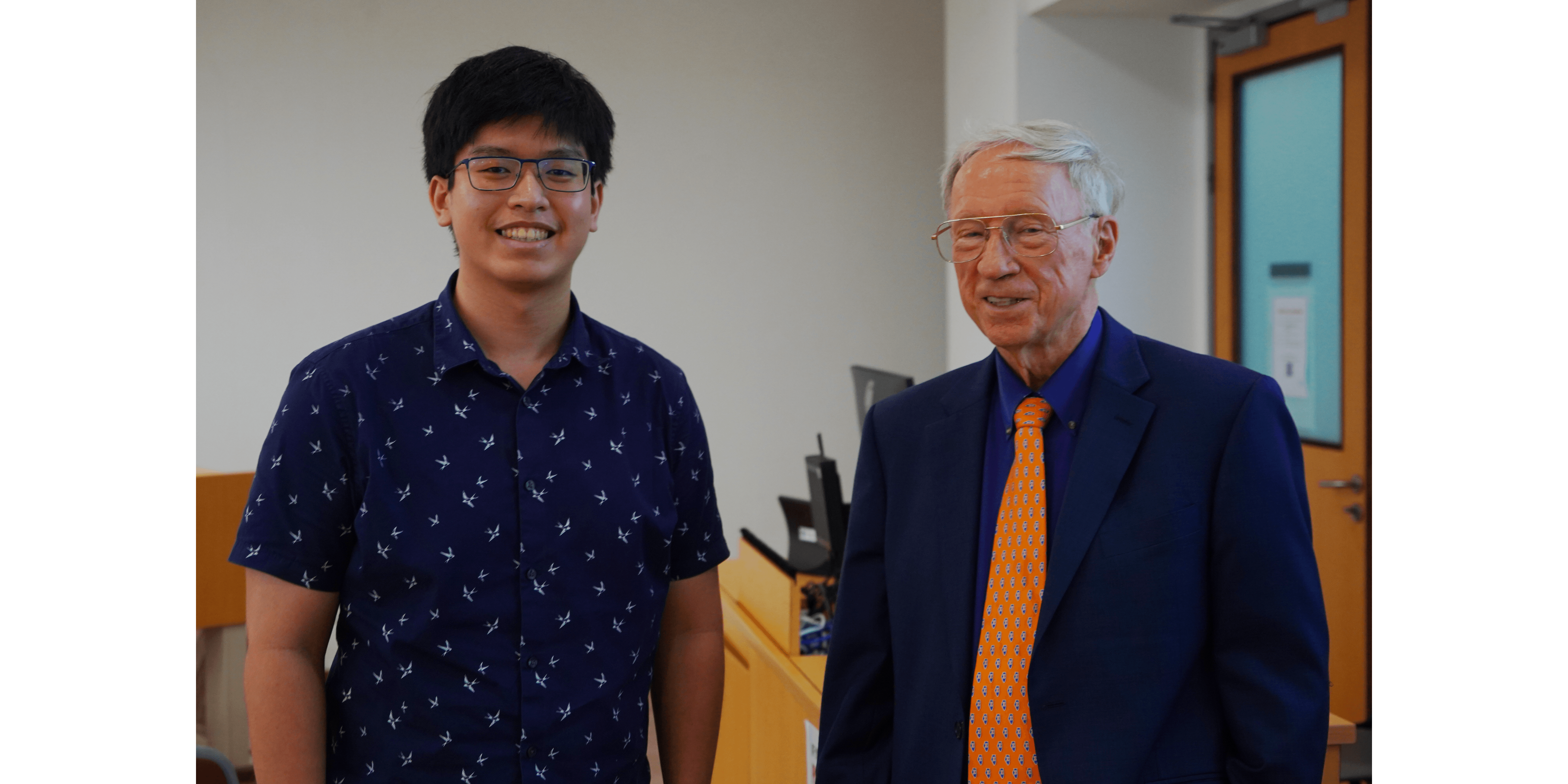
He somehow chanced upon (1), or (99) one day and was surprised that there exists a formula for the reciprocal of $\pi$ (although having $\pi^{2}$ appearing in the evaluation of $\zeta\left(2\right)$ was already unexpected). It was only in early 2023 where Thang decided to look into the formula again. He also wishes to express his gratitude to B. Berndt for their insightful correspondence and inspiring lectures during his visit to Nanyang Technological University in September 2024 (Figure 1).

Figure 1. Thang and Berndt at Nanyang Technological University (2024)

Ramanujan’s series is beautiful. A MathOverflow post by Piezas III mentions the following coincidences [8]. Recall the fundamental solution to Pell’s equation $x^{2}-29y^{2}=1$ that was discussed earlier, i.e.

(102) $$u_{29}=\frac{5+\sqrt{29}}{2},$$

and

(103) $$u_{29}^{3}=70+13\sqrt{29}\quad \text{which implies}\quad{\color[rgb]{1,0,0}\definecolor[named]{pgfstrokecolor}{rgb}{1,0,0}70}^{2}-29\cdot{\color[rgb]{1,0,0}\definecolor[named]{pgfstrokecolor}{rgb}{1,0,0}13}^{2}=-1$$

(104) $$u_{29}^{6}=9801+1820\sqrt{29}\quad \text{which implies}\quad{\color[rgb]{1,0,0}\definecolor[named]{pgfstrokecolor}{rgb}{1,0,0}9801}^{2}-29\cdot{\color[rgb]{1,0,0}\definecolor[named]{pgfstrokecolor}{rgb}{1,0,0}1820}^{2}=1$$

Also,

(105) $$2^{6}\left(u_{29}^{6}+u_{29}^{-6}\right)^{2}={\color[rgb]{1,0,0}\definecolor[named]{pgfstrokecolor}{rgb}{1,0,0}396}^{4}.$$

The number 26390 in (1) or (99) can be factorised as $29\cdot{\color[rgb]{1,0,0}\definecolor[named]{pgfstrokecolor}{rgb}{1,0,0}70}\cdot{\color[rgb]{1,0,0}\definecolor[named]{pgfstrokecolor}{rgb}{1,0,0}13}$, and looking at the big picture, we have

(106) $$\frac{1}{\pi}=\frac{2\sqrt{2}}{{\color[rgb]{1,0,0}\definecolor[named]{pgfstrokecolor}{rgb}{1,0,0}9801}}\sum_{n=0}^{\infty}\frac{29\cdot{\color[rgb]{1,0,0}\definecolor[named]{pgfstrokecolor}{rgb}{1,0,0}70}\cdot{\color[rgb]{1,0,0}\definecolor[named]{pgfstrokecolor}{rgb}{1,0,0}13}n+1103}{\left(n!\right)^{4}}\cdot\frac{\left(4n\right)!}{{\color[rgb]{1,0,0}\definecolor[named]{pgfstrokecolor}{rgb}{1,0,0}396}^{4n}}.$$

This is indeed beautiful.

At last, I have come to a closure.

References

• [1] J. Borwein P. Borwein. Pi and the AGM: A Study in Analytic Number Theory and Computational Complexity. Wiley, New York, 1987.
• [2] S. Ramanujan. Modular equations and approximations to $\pi$. Quarterly Journal of Mathematics 45 (1914), 350-372.
• [3] Borwein, J. and Bailey, D. Pi: The next generation: A sourcebook on the recent history of pi and its computation. Springer. 2016.
• [4] Borwein, J. M., Glasser, M. L., McPhedran, R. C., et al. Lattice Sums: Then and Now. Cambridge University Press. 2013.
• [5] Zucker, I. J. and M. M. Robertson. Further aspects of the evaluation of βˆ‘(m,n)β‰ (0,0)(a​m2+b​m​n+c​n2)βˆ’s\sum_{\left(m,n\right)\neq\left(0,0\right)}\left(am^{2}+bmn+cn^{2}\right)^{-s}. Mathematical Proceedings of the Cambridge Philosophical Society, vol. 95, no. 1, 1984, pp. 5–13.
• [6] Edwards, H. M. Fermat’s Last Theorem: A Genetic Introduction to Algebraic Number Theory. Graduate Texts in Mathematics. Sprigner. 2000.
• [7] Wong, C. L. On the elegance of Ramanujan’s series for $\pi$. 2021.
• [8] Piezas, T. Why do Pell equations appear in Ramanujan’s pi formulas? MathOverflow. 2014. Available at: https://mathoverflow.net/questions/189126/why-do-pell-equations-appear-in-ramanujans-pi-formulas. Accessed: 24 November 2024.